Flight Dynamics & Control

Dynamics Near Equilibria

Harry G. KwatnyDepartment of Mechanical Engineering & Mechanics

Drexel University

Outline

Program Straight & Level Flight –the primary steady-

state Perturbation Equations for Straight & Level

Flight Longitudinal & Lateral Dynamics Coordinated Turn Steady Sideslip

Program

Determine trim conditions Define and compute steady-state flight conditions Straight and level flight (cruise, climb, descend) Coordinated turn Steady sideslip

Determine perturbation models Small perturbations from a trim condition Examine dynamical behaviors

Reduction in Dimension

Notes: These properties do not require linearity These omitted variables can always be included by adding

the appropriate kinematic equations – we often include zs and/or ψ

( )

coordinates: , , , , , velocities: , , , , , 12 statesSuppose 1) the earth is flat and 2) we ignore variations of air density

the dynamics are invariant w.r.t. location , ,the dynamics a

s s s

s s s

x y z u v w p q r

x y z

φ θ ψ ⇒

⇒re invariant w.r.t. (inertial) heading

Consequently, we could drop , , , and study an 8 state systems s sx y z ψ

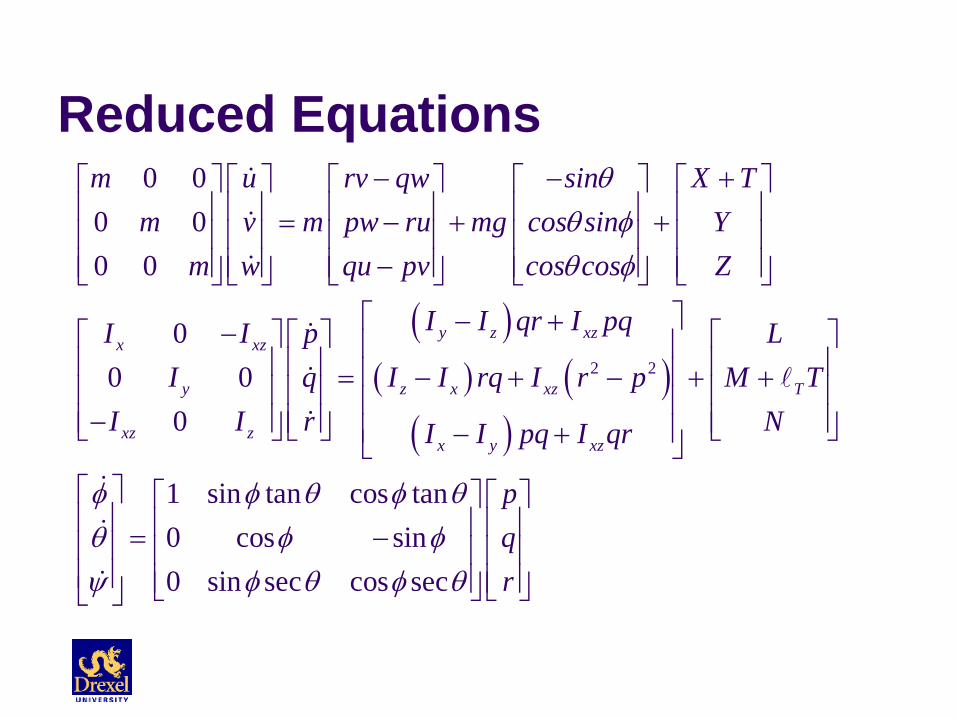
Reduced Equations

( )( ) ( )

( )

2 2

0 00 00 0

00 0

0

y z xzx xz

y z x xz

xz zx y xz

m u rv qw sin X Tm v m pw ru mg cos sin Y

m w qu pv cos cos Z

I I qr I pqI I pI q I I rq I r p

I I r I I pq I qr

θθ φθ φ

− − + = − + + −

− +− = − + − − − +

1 sin tan cos tan0 cos sin0 sin sec cos sec

T

LM T

N

pqr

φ φ θ φ θθ φ φψ φ θ φ θ

+ +

= −

Equilibria

( ) ( )( )

0 0 0

The equations are organized in first order standard form, involving the state vector , input vector , and output vector .

, state equations

, output equationsA set of values ( , , ) i

x u yE x x f x u

y h x ux u y

=

=

( )( )

0 0

0 0 0

s called an equilibrium (or trim) pointif it satisfies:

0 ,

,We are interested in motions that remain close to the equilibriumpoint.

f x u

y h x u

=

=

The Primary Steady State: Straight & Level flight

*

*

The straight and level flight condition requires equilibrium flight along a linear path with constant flight path angle , constant velocity , zero sideslip and wings level. Thus, we impose the fo

Vγ

( )( )

*

*

llowing conditions for straight and level flight:Equilibrium:

0, 0, 0 0, 0, 0 ,

0, 0, 0,Outputs:

speed:flight path angle: :sideslip: 0roll: 0

0, 0, 0 0

u v w V

p q r

V V

α β

φ θ ψ ω

γ θ α γβφ

= =

= = = = = =

= = =

=

= − ===

= =

Straight & Level Flight

( ) ( ) ( )* * * * * *

*

* * *

* *

An equilibrium point satisfying the straight and level flightconditions exists if and only if there exists , , which satisfy the equ

, , si

ations:

n 0, , , co

e

e eX V mg mg

T

T Z Vα δ α γ α

α δ

δ− + + = +

Proposition :

( )( )

* *

*

*

* * *

* * * * *

In this case the equilibrium values of the states and controls are:longitudinal variables;

states: , , 0, controls: ,lateral variables;

st

s 0,

, , ,0 0

ates:

e e

e T

V V q

M

T T

V T

α α θ γ α

α

δ

δ

β

γ

δ

α

= = = =

+ =

+ = =

+

=

=

0, 0, 0, 0, controls: 0, 0r ap r φ δ δ= = = = =

Linearization( ) ( ) ( ) ( ) ( ) ( )

( ) ( ) ( )( )( ) ( ) ( )( )

( ) ( ) ( ) ( )

( )

0 0 0

0 0 0

0 0 0

0 0 0 00 0 0 0

0 0

Define: , ,

,The equations become:

,

Now, construct a Taylor series for ,, ,

, ,

,

x t x x t u t u u t y t y y t

E x x f x x t u u t

y y t h x x t u u t

f hf x u f x u

f x x u u f x u x u hotx u

h x x u u h

δ δ δ

δ δ δ

δ δ δ

δ δ δ δ

δ δ

= + = + = +

= + +

+ = + +

∂ ∂+ + = + + +

∂ ∂

+ + =

( ) ( ) ( )

( ) ( )

( ) ( ) ( )

( ) ( )

0 0 0 00 0

0 0 0 0 0

0 0 0 00

0 0 0 0

, ,, t

Notice that , 0 and , , so

, ,

, ,

h x u h x ux u x u ho

x uf x u h x u y

f x u f x uE x x x u E x A x B ux u

y C x D uh x u h x uy x u

x u

δ δ

δ δ δ δ δ δδ δ δ

δ δ δ

∂ ∂+ + +

∂ ∂= =

∂ ∂= + = +∂ ∂ ⇒

= +∂ ∂= +

∂ ∂

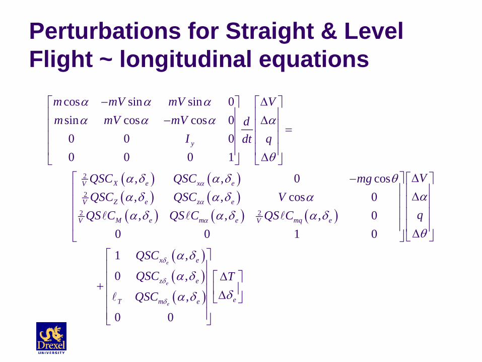
Perturbations for Straight & Level Flight ~ longitudinal equations

( ) ( )( ) ( )( ) ( ) ( )

2

2

2 2

cos sin sin 0sin cos cos 00 0 00 0 0 1

, , 0 cos, , cos 0, , , 0

0 0 1 0

y

X e x eV

Z e z eV

M e m e mq eV V

m mV mV Vm mV mV d

I qdt

VQSC QSC mgQSC QSC V

qQS C QS C QS C

α

α

α

α α αα α α α

θ

α δ α δ θαα δ α δ α

α δ α δ α δθ

− ∆ − ∆ = ∆

∆− ∆ ∆

( )( )( )

1 ,

0 ,

,

0 0

e

e

e

x e

z e

eT m e

QSC

QSC TQSC

δ

δ

δ

α δ

α δδα δ

∆ + ∆

Perturbations for Straight & Level Flight ~ lateral equations

( ) ( ) ( )( ) ( ) ( )( ) ( ) ( )

( ) ( )

2 2

2 2

2 2

0 0 00 00 00 0 0 1

cos00

0 1 tan 0

r a

r

x xy

xy z

b by y yrV V

b bl lp lrV V

b bn np nrV V

y y

l

mVI I pdI I rdt

QSC QS C QS C mu mgpQS C QS C QS CrQS C QS C QS C

C C

CQS

β β

β

β

δ δ

δ

β

φ

βα α α θα α αα α α

φθ

α α

− = −

− −

+

( ) ( )( ) ( )

0 0

a

r a

l r

an n

C

C Cδ

δ δ

α α δδα α

Longitudinal DynamicsNear straight and level flight the general equations of motion may bedivided into two sets which are almost decoupled.

Motion in body x-z plane, without yawingor rolling 0, 0,v φ= =

Longitudinal Dynamics :( )0, 0, 0 .

, , , , ,the - plane is a plane of symmetry

Uncoupled longitudinal motions exist provided rotor gyroscopic effects are absentthe flat earth approximation is v

s s

p ru w q x y

x z

ψθ

= = =

Longitudinal Variables :

alid

0 sinForce equations:

0 cosMoment equations:

cos sinKinematics: ,

sin cos

y

s

s

m u qw Xm mg

m w qu ZI q M

x uq

z v

θθ

θ θθ

θ θ

−

= + +

=

= = −

Lateral Dynamics( )* * *

motion in body x-y plane, no pitching

0, , , 0,

, , , , , motions are small-trajectory remains close to stra

Uncoupled lateral motions exist provided

s

w u u q

v p r y

θ θ α α

ψ φ

≈ ≈ = = ≈

Lateral Dynamics :

Lateral Variables :

* *

ight & levelaerodynamic cross-coupling terms are negligiblerotor gyroscopic effects are absentthe flat earth approximation is valid

Force equations: cos sin

Moment equations: x

mv mru mg YI

θ φ

= − + +

−

( )

*

*

* * *

1 cos tanKinematics:

cos sec

cos sin sin sin sin cos cos

xz

xz z

s

I p LI I r N

pr

y u v

φ θφφ θψ

θ φ φ θ ψ φ ψ

= −

=

= + +

Banked Coordinated Turn

( )

( )( )

The banked turn is defined by the following conditions:1) equilibrium - , , , , , , , are constant

0

0

y z xz

z x

V u v w p q r

rv qw sin X Tm pw ru mg cos sin Y

qu pv cos cos Z

I I qr I pq

I I r

α β

θθ φθ φ

− − + = − + + −

− +

= − ( )( )

2 2xz T

x y xz

Lq I r p M T

NI I pq I qr

+ − + + − +

Banked Coordinated Turn~2

*

*

2) banked turn condition: the (inertial) angular velocity is vertical and constant

0 sin0 cos sin

cos cos3) coordinated turn condition - sum of gravity a

s

pqr

θω θ φ ω

ω θ φ

− = ⇒ =

* *

nd inertial forces lie in plane of symmetry ( plane)

cos sin 0cos sin cos cos cos sin 0

4) climb conditions: ,

x zmpw mru mg

pV rV gV V

θ φβ α β α θ φ

γ γ

−− + = ⇒

− + =

= =

Banked Coordinated Turn ~ 3 There are 12 equations in 12 unknowns

The fact that the velocity is constant in body frame, with constant angular velocity about zs inusures that ground track is circular.

The coordinated turn condition insures that pilot and passengers will not experience any side forces.

A pilot achieves coordination by using the rudder in conjunction with an instrument called a turn coordinator which measures the difference between the inertial and gravity forces acting along the y axis.

The rudder also induces a moment which counteracts the “adverse yaw” moment resulting from increased (decreased) drag on the outside (inside) wing produced by aileron position and which can be significant during the rolling phase of the turn.

, , , , , , , , , , ,e a rV p q r Tα β θ φ δ δ δ

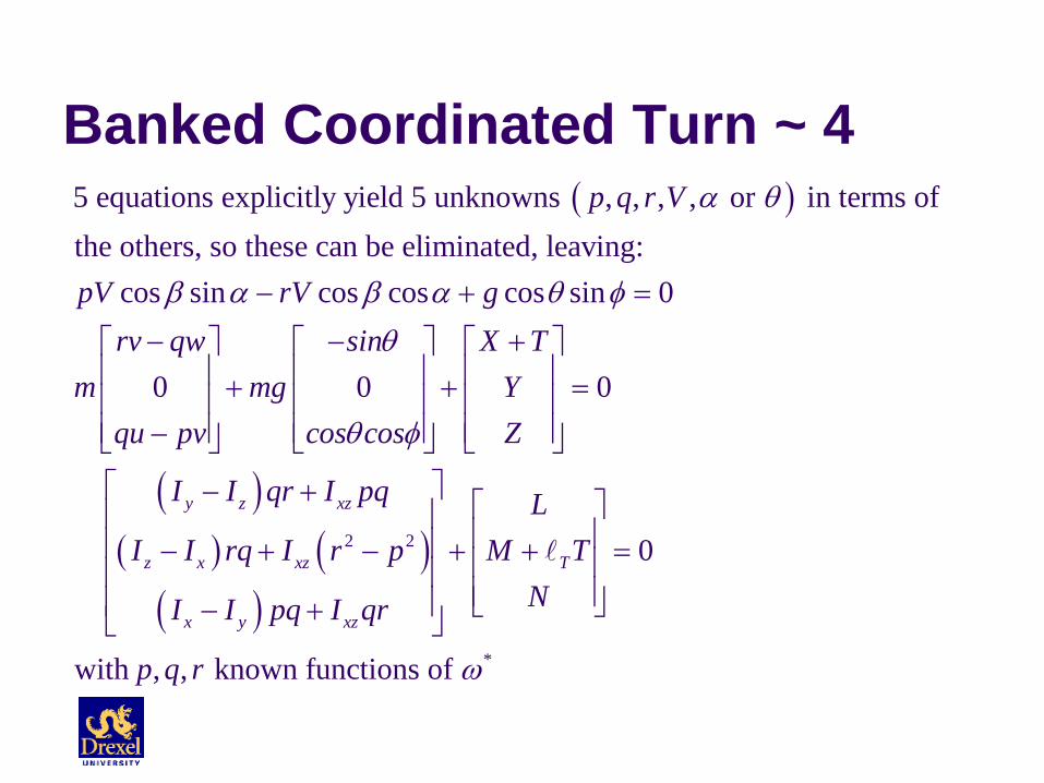
Banked Coordinated Turn ~ 4( )5 equations explicitly yield 5 unknowns , , , , or in terms of

the others, so these can be eliminated, leaving:cos sin cos cos cos sin 0

0 0

p q r V

pV rV grv qw sin X T

m mgqu pv cos cos

α θ

β α β α θ φθ

θ φ

− + =

− − + + + −

( )( ) ( )

( )

2 2

*

0

0

with , , known functions of

y z xz

z x xz T

x y xz

YZ

I I qr I pq LI I rq I r p M T

NI I pq I qr

p q r ω

=

− + − + − + + = − +

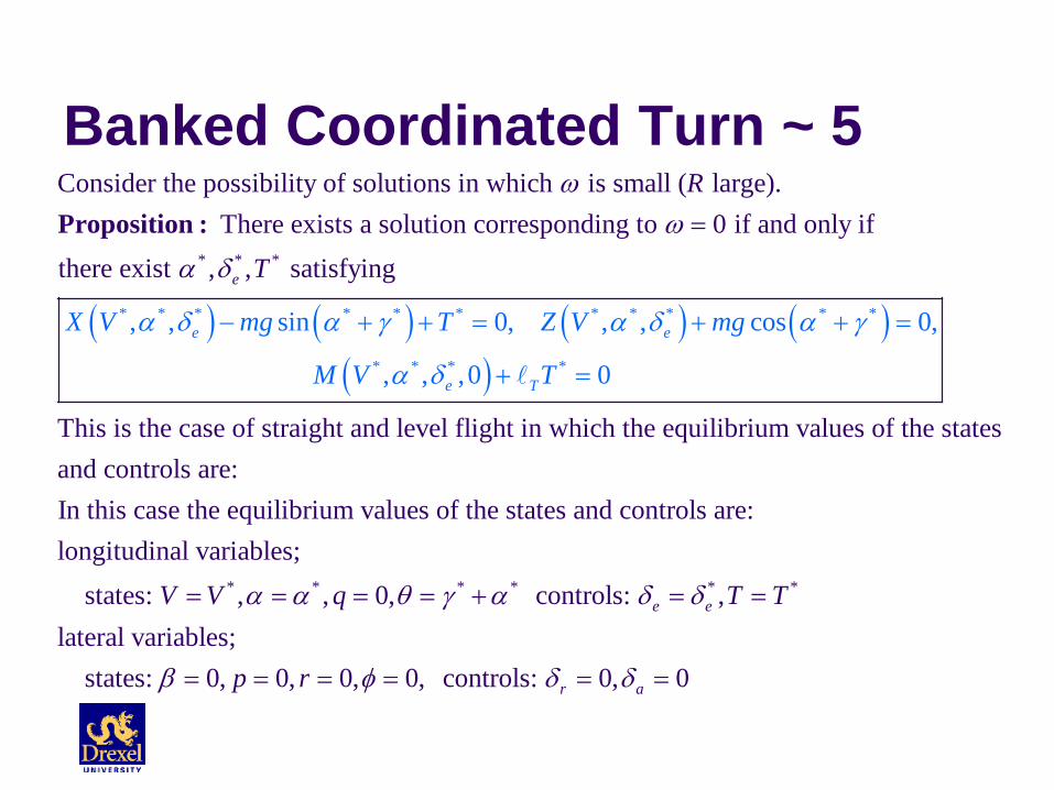
Banked Coordinated Turn ~ 5

( ) ( )* * * * * *

* * *

Consider the possibility of solutions in which is small ( large). There exists a solution corresponding to 0 if and only if

there exist , , satisfying

, , sin 0,

e

eX V mg

R

T

T Zα δ α

ωω

α

γ

δ

=

− + + =

Proposition :

( ) ( )( )

* * * * *

* * * *

This is the case of straight and level flight in which the equilibrium values of the statesand controls are:In this case the e

, , cos 0,

, , ,0 0

quilibrium values of the states

e

e T

V mg

M V T

α δ α γ

α δ

+ + =

+ =

* * * * * *

and controls are:longitudinal variables;

states: , , 0, controls: ,lateral variables;

states: 0, 0, 0, 0, controls: 0, 0

e e

r a

V V q T T

p r

α α θ γ α δ δ

β φ δ δ

= = = = + = =

= = = = = =

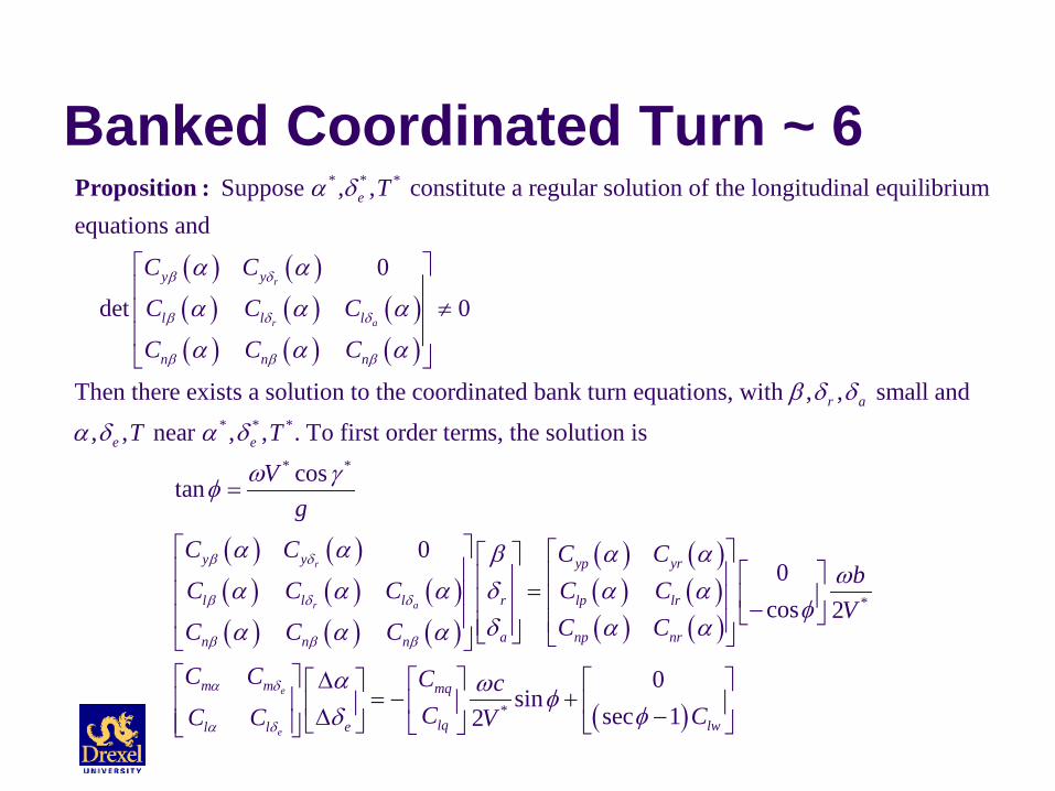
Banked Coordinated Turn ~ 6

( ) ( )( ) ( ) ( )( ) ( ) ( )

* * * Suppose , , constitute a regular solution of the longitudinal equilibriumequations and

0

det 0

Then there exists a solution to the coordina

r

r a

e

y y

l l l

n n n

T

C C

C C C

C C C

β δ

β δ δ

β β β

α δ

α α

α α α

α α α

≠

Proposition :

( ) ( )( ) ( ) ( )( ) ( ) ( )

( ) ( )( ) ( )

* * *

* *

ted bank turn equations, with , , small and

, , near , , . To first order terms, the solution is

costan

0r

r a

r a

e e

y y yp yr

l l l r lp lr

an n n

T T

Vg

C C C CC C C C C

C C C

β δ

β δ δ

β β β

β δ δ

α δ α δ

ω γφ

α α β α αα α α δ α α

δα α α

=

= ( ) ( )

( )

*

*

0cos 2

0sin

sec 12e

e

np nr

m m mq

lq lwel l

bV

C C

C C C cC CC C V

α δ

α δ

ωφ

α α

α ω φφδ

−

∆ = − + −∆

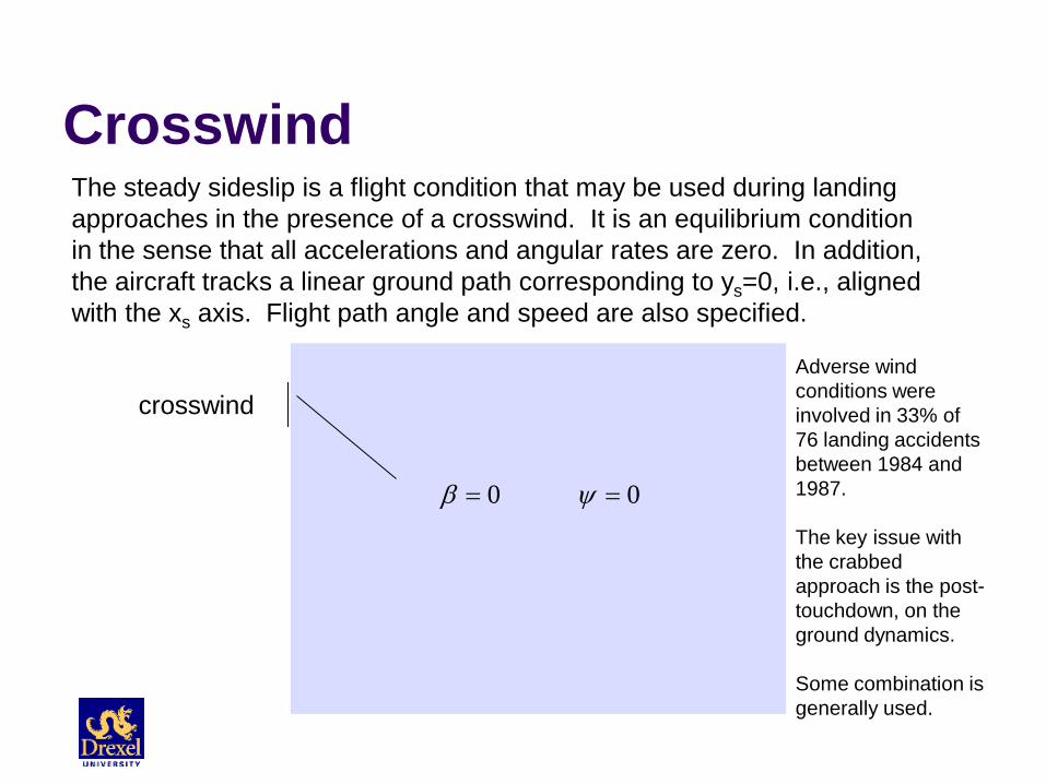
CrosswindThe steady sideslip is a flight condition that may be used during landing approaches in the presence of a crosswind. It is an equilibrium condition in the sense that all accelerations and angular rates are zero. In addition, the aircraft tracks a linear ground path corresponding to ys=0, i.e., aligned with the xs axis. Flight path angle and speed are also specified.

crosswindAdverse wind conditions were involved in 33% of 76 landing accidents between 1984 and 1987.

The key issue with the crabbed approach is the post-touchdown, on the ground dynamics.

Some combination is generally used.

0 0β ψ= =

Crosswind ~ 2

0

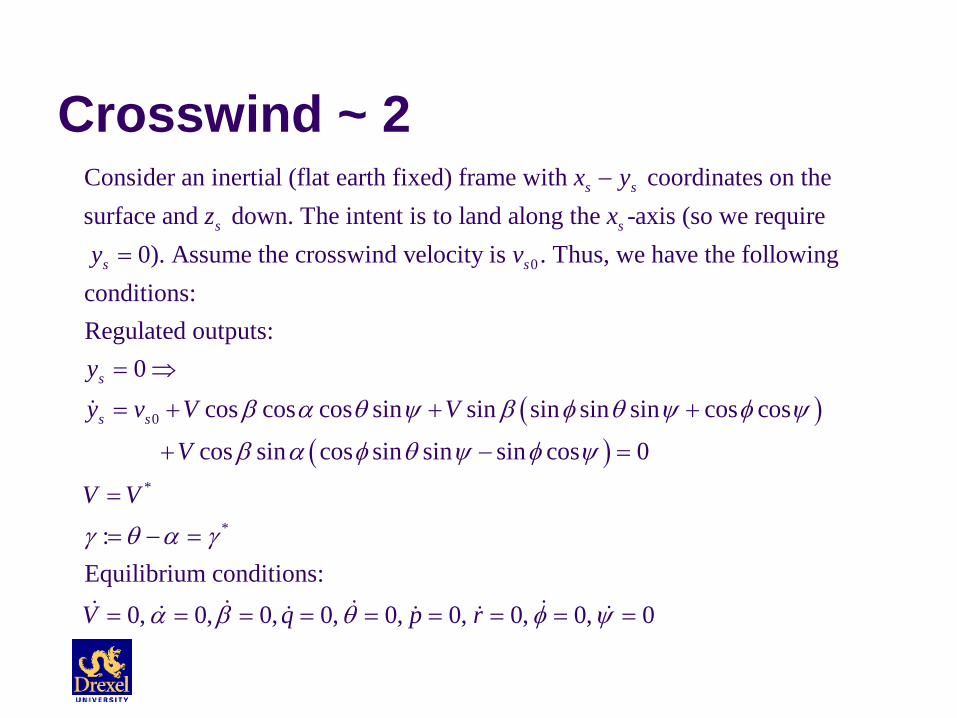
Consider an inertial (flat earth fixed) frame with coordinates on thesurface and down. The intent is to land along the -axis (so we require 0). Assume the crosswind velocity is . Thus

s s

s s

s s

x yz x

y v

−

=

( )( )

0

*

*

, we have the followingconditions:Regulated outputs:

0cos cos cos sin sin sin sin sin cos cos

cos sin cos sin sin sin cos 0

:Equilibrium conditions:

0, 0, 0, 0,

s

s s

yy v V V

V

V V

V q

β α θ ψ β φ θ ψ φ ψ

β α φ θ ψ φ ψ

γ θ α γ

α β θ

= ⇒

= + + +

+ − =

=

= − =

= = = =

0, 0, 0, 0, 0p r φ ψ= = = = =

Crosswind ~ 3

( ) ( ) ( ) ( )* * * * * * * * * *

*

*

* *

(crabbing solutions) A solution to the ground tracking problem exists with 0, 0 if and only if there exist , and which satisfy

, , sin 0, , s

:

, co

e

e eX V mg T Z V mg

T

α δ α γ α δ

β

α γ

φ α δ= =

− + + = + + =

Proposition :

( )* * * *

0* *

0,

, , ,0 0

and

1cos

s

e TM V

v

T

V

α δ

γ

+ =

≤

Crosswind ~ 4

( ) ( ) ( ) ( )* * * * * * * * * * *

*

* * *

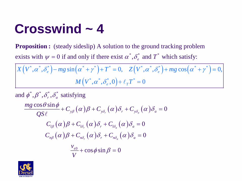
(steady sideslip) A solution to the ground tracking problem exists with 0 if and only if there exist , and which

, , sin 0, , , cos

satis y:

0,

,

f

e e

e

X V mg T Z V mg

M V

T

α δ α γ α α γ

ψ

α

δ

δ

α

− + + = + + =

=

Proposition :

( )

( ) ( ) ( )

( ) ( ) ( )( ) ( ) ( )

* * *

* * * *

0

and , , , satisfyingcos sin 0

0

0

cos

, ,0 0

sin 0

r a

r a

r a

r a

y y r y a

l l r l a

n n r n

e

s

T

a

mg C C CQS

C C C

C C C

vV

T

β δ δ

β δ δ

β δ δ

φ β δ δθ φ α β α δ α δ

α β α δ α δ

α β α δ

δ

α δ

φ β

+ + + =

+ + =

+ + =

+ =

+ =

Crosswind ExampleA hypothetical subsonic transport (adapted from Etkin) has the following data

-0.168, 0.067, 0,

-0.047, 0.003, = - 0.04,

0.3625, -0.16, -0.005

Suppose the cros

r a

r a

r a

y y y

l l l

n n n

C C C

C C C

C C C

β δ δ

β δ δ

β δ δ

= = =

= =

= = =

0swind is 0.15 . Then the following results areobtained (in degrees)

-8.59437, =-0.121212, -19.7409, 8.61781Slip to the left, roll to the left, hard right rudder, left aileron (into wind)

r a

v V

β φ δ δ

=

= = =

Comments from Airbus Pilots “I do not find crosswinds to be anymore challenging in this

airplane than any other. You have to understand that you cannot "slip" this airplane because your are commanding a ROLL RATE with the Side Stick Controller, not a BANK ANGLE. Here is a suggestion: Allow the airplane to do an Auto Land in a crosswind when it is convenient, and VFR. You will be shocked at the timing of when the airplane leaves the CRAB and applies rudder to align the nose parallel with the runway. You think it just isn't going to do it, and at the very last second, it slides it in perfectly. I would guess in the last 20 feet or less. My technique is just the same as any airplane I've ever flown. C-150 to B-767. Crab it down to the flare, apply enough rudder to straighten the nose, drop the up-wind wing to prevent drift, land on the up-wind main first.” -- 5-Year Airbus Captain.