HAL Id: hal-00296966https://hal.archives-ouvertes.fr/hal-00296966

Submitted on 26 Sep 2006

HAL is a multi-disciplinary open accessarchive for the deposit and dissemination of sci-entific research documents, whether they are pub-lished or not. The documents may come fromteaching and research institutions in France orabroad, or from public or private research centers.

L’archive ouverte pluridisciplinaire HAL, estdestinée au dépôt et à la diffusion de documentsscientifiques de niveau recherche, publiés ou non,émanant des établissements d’enseignement et derecherche français ou étrangers, des laboratoirespublics ou privés.

Flood routing modelling with Artificial Neural NetworksR. Peters, G. Schmitz, J. Cullmann

To cite this version:R. Peters, G. Schmitz, J. Cullmann. Flood routing modelling with Artificial Neural Networks. Ad-vances in Geosciences, European Geosciences Union, 2006, 9, pp.131-136. <hal-00296966>

Adv. Geosci., 9, 131–136, 2006www.adv-geosci.net/9/131/2006/© Author(s) 2006. This work is licensedunder a Creative Commons License.

Advances inGeosciences

Flood routing modelling with Artificial Neural Networks

R. Peters, G. Schmitz, and J. Cullmann

Institute of Hydrology and Meteorology, University of Technology, Dresden, Germany

Received: 23 January 2006 – Revised: 22 May 2006 – Accepted: 3 July 2006 – Published: 26 September 2006

Abstract. For the modelling of the flood routing in thelower reaches of the Freiberger Mulde river and its tributariesthe one-dimensional hydrodynamic modelling system HEC-RAS has been applied. Furthermore, this model was used togenerate a database to train multilayer feedforward networks.

To guarantee numerical stability for the hydrodynamicmodelling of some 60 km of streamcourse an adequate res-olution in space requires very small calculation time steps,which are some two orders of magnitude smaller than the in-put data resolution. This leads to quite high computation re-quirements seriously restricting the application – especiallywhen dealing with real time operations such as online floodforecasting.

In order to solve this problem we tested the applicationof Artificial Neural Networks (ANN). First studies showthe ability of adequately trained multilayer feedforward net-works (MLFN) to reproduce the model performance.

1 Introduction

Recent extreme flood events in central Europe, e.g. the floodof August 2002, which affected – amongst others – the catch-ment of the Freiberger Mulde river, led to an increased de-mand for fast and robust prediction tools.

The proper modelling of flood wave propagation faceschallenges like backwater effects at river junctions and widefloodplains. To take this into account sophisticated hydro-dynamic modelling is necessary. We applied the HEC-RiverAnalysis System (HEC-RAS), which is a one-dimensionalhydrodynamic model based on a numerical solution of theSt-Venant-equations. This allows – and requires – the useof detailed topographical information representing the hy-draulic properties of the river reaches. The river bed and the

Correspondence to:R. Peters(ronny.peters@tu-dresden.de)

floodplains are described by geometrical data and roughnessparameters of representative cross sections. Obviously, theaccuracy of the model is related to the distance between thecross sections.

To avoid numerical instabilities a high resolution in spacerequires a small computation interval. This relationship is de-scribed by the Courant criterion. In this study a mean crosssection distance of some 150 m corresponded to time steps ofabout 15 seconds. This leads to relatively high computationalefforts. That is the reason why in case of real time operationsthe application of such a highly sophisticated model is notvery functional. For this purpose fully robust and fast simu-lation tools like ANN is needed.

Previous studies concerning the application of ANN forthe simulation of routing processes only used observed data.Shrestha et al. (2005) trained MLFN for the purpose of floodflow simulation at the Neckar river using a hydrodynamic nu-merical model, but only to provide data for unobserved loca-tions for historical flood events. The main problem remainsthe lack of extrapolation capability. Or, as stated by Minnsand Hall (1996): “ANN are a prisoner of their training data”.We used hydrodynamic modelling to generate a database forthe training of the MLFN covering the whole range of possi-ble flood events. This guaranties the capability of the trainedMLFN to predict extreme events beyond recorded floods.

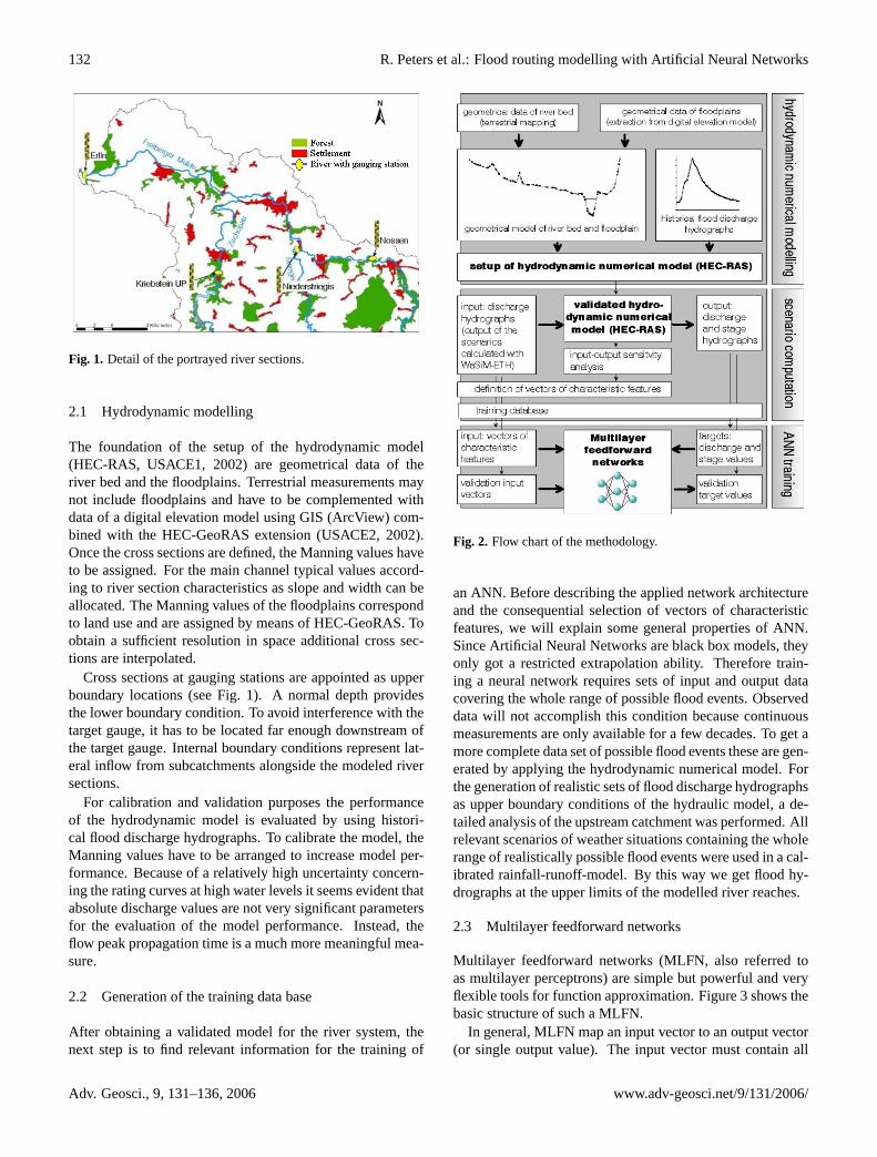
The methodology was successfully tested at the lower riverreaches of the Freiberger Mulde catchment (Fig. 1).

2 Methodology

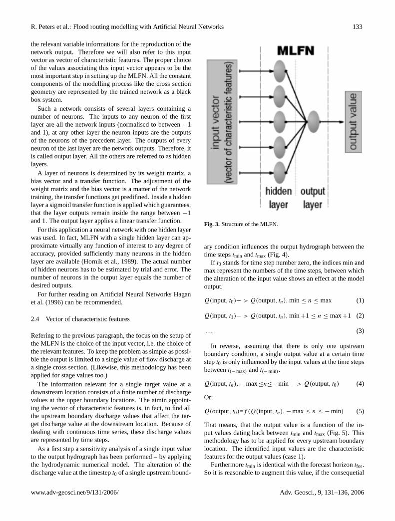
A general description of the methodology in the form of aflow chart is showed in Fig. 2. In the following the particularsteps will be portrayed in detail.

Published by Copernicus GmbH on behalf of the European Geosciences Union.

132 R. Peters et al.: Flood routing modelling with Artificial Neural Networks

Fig. 1. Detail of the portrayed river sections.

2.1 Hydrodynamic modelling

The foundation of the setup of the hydrodynamic model(HEC-RAS, USACE1, 2002) are geometrical data of theriver bed and the floodplains. Terrestrial measurements maynot include floodplains and have to be complemented withdata of a digital elevation model using GIS (ArcView) com-bined with the HEC-GeoRAS extension (USACE2, 2002).Once the cross sections are defined, the Manning values haveto be assigned. For the main channel typical values accord-ing to river section characteristics as slope and width can beallocated. The Manning values of the floodplains correspondto land use and are assigned by means of HEC-GeoRAS. Toobtain a sufficient resolution in space additional cross sec-tions are interpolated.

Cross sections at gauging stations are appointed as upperboundary locations (see Fig. 1). A normal depth providesthe lower boundary condition. To avoid interference with thetarget gauge, it has to be located far enough downstream ofthe target gauge. Internal boundary conditions represent lat-eral inflow from subcatchments alongside the modeled riversections.

For calibration and validation purposes the performanceof the hydrodynamic model is evaluated by using histori-cal flood discharge hydrographs. To calibrate the model, theManning values have to be arranged to increase model per-formance. Because of a relatively high uncertainty concern-ing the rating curves at high water levels it seems evident thatabsolute discharge values are not very significant parametersfor the evaluation of the model performance. Instead, theflow peak propagation time is a much more meaningful mea-sure.

2.2 Generation of the training data base

After obtaining a validated model for the river system, thenext step is to find relevant information for the training of

Fig. 2. Flow chart of the methodology.

an ANN. Before describing the applied network architectureand the consequential selection of vectors of characteristicfeatures, we will explain some general properties of ANN.Since Artificial Neural Networks are black box models, theyonly got a restricted extrapolation ability. Therefore train-ing a neural network requires sets of input and output datacovering the whole range of possible flood events. Observeddata will not accomplish this condition because continuousmeasurements are only available for a few decades. To get amore complete data set of possible flood events these are gen-erated by applying the hydrodynamic numerical model. Forthe generation of realistic sets of flood discharge hydrographsas upper boundary conditions of the hydraulic model, a de-tailed analysis of the upstream catchment was performed. Allrelevant scenarios of weather situations containing the wholerange of realistically possible flood events were used in a cal-ibrated rainfall-runoff-model. By this way we get flood hy-drographs at the upper limits of the modelled river reaches.

2.3 Multilayer feedforward networks

Multilayer feedforward networks (MLFN, also referred toas multilayer perceptrons) are simple but powerful and veryflexible tools for function approximation. Figure 3 shows thebasic structure of such a MLFN.

In general, MLFN map an input vector to an output vector(or single output value). The input vector must contain all

Adv. Geosci., 9, 131–136, 2006 www.adv-geosci.net/9/131/2006/

R. Peters et al.: Flood routing modelling with Artificial Neural Networks 133

the relevant variable informations for the reproduction of thenetwork output. Therefore we will also refer to this inputvector as vector of characteristic features. The proper choiceof the values associating this input vector appears to be themost important step in setting up the MLFN. All the constantcomponents of the modelling process like the cross sectiongeometry are represented by the trained network as a blackbox system.

Such a network consists of several layers containing anumber of neurons. The inputs to any neuron of the firstlayer are all the network inputs (normalised to between−1and 1), at any other layer the neuron inputs are the outputsof the neurons of the precedent layer. The outputs of everyneuron of the last layer are the network outputs. Therefore, itis called output layer. All the others are referred to as hiddenlayers.

A layer of neurons is determined by its weight matrix, abias vector and a transfer function. The adjustment of theweight matrix and the bias vector is a matter of the networktraining, the transfer functions get predifined. Inside a hiddenlayer a sigmoid transfer function is applied which guarantees,that the layer outputs remain inside the range between−1and 1. The output layer applies a linear transfer function.

For this application a neural network with one hidden layerwas used. In fact, MLFN with a single hidden layer can ap-proximate virtually any function of interest to any degree ofaccuracy, provided sufficiently many neurons in the hiddenlayer are available (Hornik et al., 1989). The actual numberof hidden neurons has to be estimated by trial and error. Thenumber of neurons in the output layer equals the number ofdesired outputs.

For further reading on Artificial Neural Networks Haganet al. (1996) can be recommended.

2.4 Vector of characteristic features

Refering to the previous paragraph, the focus on the setup ofthe MLFN is the choice of the input vector, i.e. the choice ofthe relevant features. To keep the problem as simple as possi-ble the output is limited to a single value of flow discharge ata single cross section. (Likewise, this methodology has beenapplied for stage values too.)

The information relevant for a single target value at adownstream location consists of a finite number of dischargevalues at the upper boundary locations. The aimin appoint-ing the vector of characteristic features is, in fact, to find allthe upstream boundary discharge values that affect the tar-get discharge value at the downstream location. Because ofdealing with continuous time series, these discharge valuesare represented by time steps.

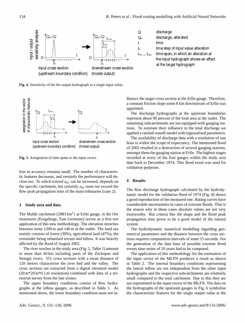
As a first step a sensitivity analysis of a single input valueto the output hydrograph has been performed – by applyingthe hydrodynamic numerical model. The alteration of thedischarge value at the timestept0 of a single upstream bound-

Fig. 3. Structure of the MLFN.

ary condition influences the output hydrograph between thetime stepstmin andtmax (Fig. 4).

If t0 stands for time step number zero, the indices min andmax represent the numbers of the time steps, between whichthe alteration of the input value shows an effect at the modeloutput.

Q(input, t0)− > Q(output, tn), min ≤ n ≤ max (1)

Q(input, t1)− > Q(output, tn), min+1 ≤ n ≤ max+1 (2)

. . . (3)

In reverse, assuming that there is only one upstreamboundary condition, a single output value at a certain timestept0 is only influenced by the input values at the time stepsbetweent(− max) andt(− min).

Q(input, tn), − max≤n≤− min− > Q(output, t0) (4)

Or:

Q(output, t0)=f (Q(input, tn),− max≤ n ≤ − min) (5)

That means, that the output value is a function of the in-put values dating back betweentmin and tmax (Fig. 5). Thismethodology has to be applied for every upstream boundarylocation. The identified input values are the characteristicfeatures for the output values (case 1).

Furthermoretmin is identical with the forecast horizontfor.So it is reasonable to augment this value, if the consequetial

www.adv-geosci.net/9/131/2006/ Adv. Geosci., 9, 131–136, 2006

134 R. Peters et al.: Flood routing modelling with Artificial Neural Networks

Fig. 4. Sensitivity of the the output hydrograph to a single input value.

Fig. 5. Assignation of time spans to the input vector.

loss in accuracy remains small. The number of characteris-tic features decreases, and certainly the performance will de-cline too. To which extendtfor can be increased, depends onthe specific catchment, but certainlytfor must not exceed theflow peak propagation time of the main tributaries (case 2).

3 Study area and data

The Mulde catchment (2983 km2) at Erlln gauge, in the Oremountains (Erzgebirge, East Germany) serves as a first testapplication of this new methodology. The elevation stretchesbetween some 1200 m and 140 m at the outlet. The land usemainly consists of forest (30%), agricultural land (47%), theremainder being urbanised terrain and fallow. It was heavilyaffected by the flood of August 2002.

The river reaches in the study area (Fig. 1, Table 1) amountto more than 60 km including parts of the Zschopau andStriegis rivers. 551 cross sections with a mean distance of120 metres characterise the river bed and the valley. Thecross sections are extracted from a digital elevation model(20 m*20 m*0.1 m resolution) combined with data of a ter-restrial survey from the late sixties.

The upper boundary conditions consist of flow hydro-graphs at the inflow gauges, as described in Table 1. Asmentioned above, the lower boundary condition must not in-

fluence the target cross section at the Erlln gauge. Therefore,a constant friction slope some 8 km downstream of Erlln wasappointed.

The discharge hydrographs at the upstream boundariesrepresent about 90 percent of the total area at the outlet. Theremaining subcatchments are not equipped with gauging sta-tions. To estimate their influence to the total discharge weapplied a rainfall-runoff-model with regionalised parameters.

The availability of discharge data with a resolution of onehour is within the scope of expectancy. The mentioned floodof 2002 resulted in a destruction of several gauging stations,amongst them the gauging station at Erlln. The highest stagesrecorded at every of the four gauges within the study areadate back to December 1974. This flood event was used forvalidation purposes.

4 Results

The flow discharge hydrograph calculated by the hydrody-namic model for the validation flood of 1974 (Fig. 8) showsa good reproduction of the measured one. Rating curves haveconsiderable uncertainties in cases of extreme floods. That isthe reason why in these cases absolute values are not verytrustworthy. But criteria like the shape and the flood peakpropagation time prove to be a good model of the naturalsystem.

The hydrodynamic numerical modelling regarding geo-metrical parameters and the distance between the cross sec-tions requires computation intervals of some 15 seconds. Forthe generation of the data base of possible extreme floodevents time series of 20 years had to be computed.

The application of this methodology for the estimation ofthe input vector of the MLFN produces a result as shownin Table 2. The internal boundary conditions representingthe lateral inflow are not independent from the other inputhydrographs and the respective subcatchments are relativelysmall compared to the total catchment. Due to this they arenot represented in the input vector of the MLFN. The dots onthe hydrographs of the upstream gauges in Fig. 6 symbolisethe characteristic features for the single output value at the

Adv. Geosci., 9, 131–136, 2006 www.adv-geosci.net/9/131/2006/

R. Peters et al.: Flood routing modelling with Artificial Neural Networks 135

Table 1. Catchment characteristics of the study area.

Upper boundaries:

Gauge Tributary Area [km2] Mean flow [m3/s]

Kriebstein UP Zschopau 1757 24Nossen Freiberger Mulde 585 7Niederstriegis Striegis 283 2.7

Lower boundary:

Constant friction slope some 8 km downsteam of the target gauge at Erlln

Table 2. Propagation times to the Erlln gauging station.

Gauge Peak propagation time Influence interval

Kriebstein 6 h 3–9 hNossen 8 h 6–9 hNiederstriegis 6 h 6–7 h

Fig. 6. Characteristic features (blue dots) for the target dischargevalue (red dot).

target hydrograph (case 1). Reducing this set by the unfilleddots keeps only values within a distance of at least 6 h (min-imum flood peak propagation time) to the target value (case2).

For both cases MLFN with 15 neurons in the hidden layerwere trained. Figure 7 shows a comparison of the networkoutputs and the outputs of the hydrodynamic model (hereinreferred to as targets) as normalised values. The mapped datahave not been used as training data. In both cases an excellentperformance of the trained MLFN can be reported.

Figure 8 compares the output of the MLFN (case 2) withthe output of the hydrodynamic model and the measured hy-drograph for the 1974 flood event. The trained MLFN is ableto reproduce the performance of the physically based modelto a satisfying degree of precision.

Fig. 7. Correlation of MLFN output with output of HEC-RAS, left:case 1, right: case 2).

Fig. 8. Performances of HEC-RAS and the MLFN for the floodevent of 1974.

Moreover, the application of the MLFN is much faster thanHEC-RAS. The calculation of a time series of one year takesless than a second, compared to about 12 h with the hydrody-namic numerical model.

www.adv-geosci.net/9/131/2006/ Adv. Geosci., 9, 131–136, 2006

136 R. Peters et al.: Flood routing modelling with Artificial Neural Networks

5 Conclusions

This contribution presented a new methodology to com-bine hydrodynamic numerical modelling with artificial intel-ligence. The goal is to overcome both the restricted extrap-olation capabilities of artificial neural networks and the highcomputation requirements concerning the application of so-phisticated physically based modelling. The advantages ofthe use of ANN for flood prediction purposes have been em-phasised. Notwithstanding, the ability of a hydrodynamicmodel to deal with extreme floods beyond recorded eventshas been incorporated.

Moreover, the hydrodynamic numerical model is an ap-propriate tool to find the characteristic features for the inputvector of the MLFN. This is the basis for an efficient utilisa-tion of the input information.

In fact, the trained MLFN reproduces the model perfor-mance in an excellent manner. The advantages of the use ofartificial intelligence are obvious: A noticeable decrease ofcomputation time may be useful for on-line flood forecast-ing. Furthermore, by reducing the vector of characteristicfeatures the forecast horizon can be increased up to the flowpeak propagation time.

Edited by: R. Barthel, J. G̈otzinger, G. Hartmann, J. Jagelke,V. Rojanschi, and J. Wolf

Reviewed by: anonymous referees

References

Hagan, M. T., Demuth, H. B., and Beale, M.: Neural Network De-sign, PWS Publishing Company, Boston, 1996.

Hornik, K. M., Stinchcombe, M., and White, H.: Multilayer feed-forward networks are universal approximators, Neural Networks,2, 5, 359–366, 1989.

Minns, A. W. and Hall, M. J.: Artificial neural networks as rainfall-runoff models, Hydrol. Sci., 41, 399–417, 1996.

Shrestha, R. R., Theobald, S., and Nestmann, F.: Simulation offlood flow in a river system using artificial neural networks, Hy-drol. Earth Syst. Sci., 9(4), 313–321, 2005.

USACE1: US-Army Corps of Engineers, HEC-River Analysis Sys-tem. Hydraulic Reference Manual, Version 3.1,http://www.hec.usace.army.mil/software/hec-ras/, 2002.

USACE2: US-Army Corps of Engineers. HEC-GeoRAS, An exten-sion for support of HEC-RAS using ArcView,http://www.hec.usace.army.mil/software/hec-ras/, 2002.

Adv. Geosci., 9, 131–136, 2006 www.adv-geosci.net/9/131/2006/