FLORIDA INTERNATIONAL UNIVERSITY

Miami, Florida

THE SUCCESSIONAL DYNAMICS OF LIGHTNING-INITIATED CANOPY GAPS

IN THE MANGROVE FORESTS OF SHARK RIVER, EVERGLADES NATIONAL

PARK, USA

A dissertation submitted in partial fulfillment of the

requirements for the degree of

DOCTOR OF PHILOSOPHY

in

BIOLOGY

by

Kevin Richard Terrence Whelan

2005

To: Interim Dean Mark Szuchman College of Arts and Sciences

This dissertation, written by Kevin Richard Terrence Whelan, and entitled The Successional Dynamics of Lightning-initiated Canopy Gaps in the Mangrove Forests of Shark River, Everglades National Park, USA, having been approved in respect to style and intellectual content, is referred to you for judgment.

We have read this dissertation and recommend that it be approved.

_______________________________________ Dr. Thomas J. Smith

_______________________________________

Dr. David W. Lee

_______________________________________ Dr. Daniel Childers

_______________________________________

Dr. Michael McClain

_______________________________________ Dr. Steven F. Oberbauer, Major Professor

Date of Defense: July 7, 2005

The dissertation of Kevin Richard Terrence Whelan is approved.

_______________________________________ Interim Dean Mark Szuchman College of Arts and Sciences

_______________________________________ Dean Douglas Wartzok

University Graduate School

Florida International University, 2005

ii

DEDICATION

I dedicate this dissertation to my family. My wife, Tina, who has read so

many versions of this work, helped me in the field, and listened to me rant about

life. She was always there for a push in the right direction or a hug, whichever

was needed. This work would not have happened without her constant

encouragement. To my daughter, Josie, who will be charged to have wise

stewardship over this planet using our limited and flawed knowledge. To my

father, Michael Whelan, who encouraged me to get a good education and always

wondered how I had a job that allowed me to play in the woods. To my mother,

Donna Whelan, who early on dragged me out to the garden, exposing me to the

wonders of nature. She always encouraged me to do what I enjoyed. To my

brother, Mike Whelan, with whom I experienced numerous explorations of nature,

during our inquisitive youth, fishing, swimming, and camping in the Everglades.

He always had the courage to try new things, towing me along with him. To the

loving memory of my grandmother and mother2, Betty Jephson and Nancy

Ugarte, two grand ladies, who taught me to love life and family the most. Finally,

this dissertation is dedicated to the resilience of the Everglades. Specifically to a

forest that has been logged, repeatedly impacted by hurricanes, starved for water

or excessively flooded, ignored and violated yet remains wild, beautiful and

always educating the curious souls that wander through it.

iii

ACKNOWLEDGMENTS

This work was supported by the Global Climate Change Program of the

U.S. Geological Survey / Biological Resources Discipline and the Department of

Interior’s “Critical Ecosystems Studies Initiative” administered by Everglades

National Park (Interagency agreement #IA5280-7-9023). Additional financial

support was provided by the Florida Integrated Science Center of the U.S.

Geological Survey specifically Jeff Keay, Dr. Russ Hall, and Dr. Ronnie Best.

Sampling occurred under Everglades National Park permit EVER-2002-SCI-0029

and EVER-2003-SCI-0056.

There were numerous folks that were roped into assisting in the field or in

the lab processing samples, data entry, or in statistical consultation, pushing

boats off mud banks and feeding the mosquitoes. I would like to deeply thank

the Mangrove Liberation Army whose members include: Laura Hadden, Jay C.

Portnoy, Justin Akeung, Lisa Maria Figaro, Benny Luedike, Augustina Lopez,

Susana Toledo, Pablo Valdes, Lisely Jimenez, Wilfred Guerreo, Marlene Dow,

Eddie Gibson, Greg Ward, Christa Walker, Jed Redwine, and Danielle Palow.

The large Dutch influx of volunteers to the MLA: Ives van Leth, Bram de Vlieger,

Bart Hafkemeijer, Arnoud van Lockant, Bram Dittrich, Camille Vogel, Chris

Duynhoven, Mark de Kwaadsteniet, Sjoerd Verhagen, Thijs Sandrink, Thijs van

Oosterhout, Tim Aalten, Tom Basten, Wiestke van Betuw, and Wouter

Woortman. GIS assistance from Pablo Ruiz and Paul Teague.

I would especially like to thank Matthew Warren, Robert Muxo, and Henry

Barreras for being there for all of the hair brain field sampling ideas, and never

iv

telling me to walk the plank. My compatriot, Gordon Anderson, for all of the help

and no reality checks, when it came to surviving the Everglades Mangroves

(leave the car keys on the tire). Philippe Hensel and Chad Husby for statistical

consultation. Assistance with manuscript editing from Cristina A. Ugarte-Whelan,

Rene Price, David Lee, Michael McClain, Dan Childers, and the Ecosystem

Review Group was greatly appreciated. Jim Lynch, for all of the SET technology

and equipment, graphics assistance, and number one abilities. Don Cahoon for

the introduction to the SET world and converting me into the fold of users of the

latest SET technology. Thanks to Ken Krauss for being a sounding board for

mangrove ecology and surviving in the federal research world. Boyd and

Charles (Flamingo Boat Mechanics) for all of the help keeping boats afloat in

times of crises.

Finally, the most wholehearted thanks to the dynamic duo that did not let

reality set in and agree to have a student work on “lightning gaps” – (the name

says it all). Liability was not an issue. Tom Smith supported and encouraged my

mangrove research, and gave me guidance on how to act like a mentor. His

straight shooting critiques of the work were useful (Though I still hate the red

pen.). He was always there to supply the resources needed to accomplish

fieldwork in the remote western Everglades. To Steve Oberbauer, my mentor

and friend, many years of water have passed under the bridge and have finally

come to an end. An undergrad hired to help out in the field never left your lab

and will always feel that you wanted the best for his students. Thanks for all of

the opportunities, advice, and encouragement.

v

Mention of trade names does not constitute endorsement by the US

Government. The author takes full responsibility for any errors or oversights in

this manuscript.

vi

ABSTRACT OF THE DISSERTATION

THE SUCCESSIONAL DYNAMICS OF LIGHTNING-INITIATED CANOPY GAPS

IN THE MANGROVE FORESTS OF SHARK RIVER, EVERGLADES NATIONAL

PARK, USA

by

Kevin Richard Terrence Whelan

Florida International University, 2005

Miami, Florida

Professor Steven F. Oberbauer, Major Professor

Gap succession is a significant determinant of structure and development

in most forest communities. Lightning strikes are an important source of canopy

gaps in the mangrove forest of Everglades National Park. I investigated the

successional dynamics of lightning-initiated canopy gaps to determine their

influence on forest stand structure of the mixed mangrove forests (Rhizophora

mangle, Laguncularia racemosa, and Avicennia germinans) of the Shark River. I

measured gap size, gap shape, light environment, soil characteristics, woody

debris, and fiddler crab abundance. I additionally measured the vegetative

composition in a chronosequences of gap successional stages (new, recruiting,

and growing gaps). I recorded survivorship, recruitment, growth and soil

elevation dynamics within a subset of new and growing gaps. I determined the

relationship between intact forest soil elevation and site hydrology in order to

interpret the effects of lightning disturbance on soil elevation dynamics.

vii

Gap size averaged 289 ± 20 m2 (± 1SE) and light transmittance decreased

exponentially as gaps filled with saplings. Fine woody debris was highest in

recruiting gaps. Soil strength was lower in the gaps than in the forest. The

abundance of large and medium fiddler crab burrows increased linearly with total

seedling abundance. Soil surface elevation declined in newly formed lightning

gaps; this loss was due to a combination of superficial erosion (8.5 mm) and

subsidence (60.9 mm). A distinct two-cohort recruitment pattern was evident in

the seedling/sapling surveys, suggesting a partitioning of the succession

between individuals present before and after lightning strike. In new gaps, the

seedling recruitment rate was twice as high as in forest and the sapling

population increased. At the growing gap stage, R. mangle seedling mortality

was 10 times greater and sapling mortality was 13 times greater than

recruitment. Growing gaps had reduced seedling stem elongation, sapling

growth and adult growth. However, a few individuals (R. mangle saplings) were

able to recruit into the adult life stage. In conclusion, the high density of R.

mangle seedlings and saplings imply that lightning strike disturbances in these

mangrove forests favor their recruitment over that of A. germinans and L.

racemosa.

viii

TABLE OF CONTENTS CHAPTER PAGE Chapter I............................................................................................................... 1

Introduction ....................................................................................................... 1 Overall dissertation objective: ........................................................................... 5 Specific research objectives covered in the dissertation:.................................. 6 Literature cited .................................................................................................. 8

Chapter II............................................................................................................ 12

Succession of lightning-initiated canopy gaps in a Neo-subtropical mangrove forest. ............................................................................................. 12 Abstract........................................................................................................... 12 Introduction ..................................................................................................... 13 Methods .......................................................................................................... 17

Study area ................................................................................................... 17 Gap definition .............................................................................................. 17 Gap environmental characteristics .............................................................. 20 Data analysis............................................................................................... 24

Results ............................................................................................................ 26 Gap environmental characteristics .............................................................. 26 Species-specific density and biomass......................................................... 33

Discussion....................................................................................................... 35 Characteristics of gap successional stages................................................. 35 Compiling a conceptual model of lightning gap succession......................... 41 Implications of lightning gaps on mangrove forest structure........................ 42

Acknowledgments........................................................................................... 46 Literature cited ................................................................................................ 47

Chapter III........................................................................................................... 72

Mangrove survival, growth, and recruitment in lightning-initiated canopy gaps and closed forest sites in Everglades National Park, Florida USA. ........ 72 Abstract........................................................................................................... 72 Introduction ..................................................................................................... 73 Methods .......................................................................................................... 74

Study area ................................................................................................... 74 Data analysis............................................................................................... 78

Results ............................................................................................................ 79 Propagules .................................................................................................. 79 Seedlings..................................................................................................... 80 Saplings....................................................................................................... 82 Adults .......................................................................................................... 84

Discussion....................................................................................................... 87 Closed canopy forest stand structure and growth ....................................... 87 New gaps versus intact forest ..................................................................... 91

ix

Growing gaps versus intact forest ............................................................... 96 Conclusion ...................................................................................................... 98 Acknowledgments......................................................................................... 100 Literature Cited: ............................................................................................ 101

Chapter IV ........................................................................................................ 118

Recent lightning-initiated Neotropical mangrove forest canopy gaps decline in soil surface elevation. ................................................................... 118 Abstract......................................................................................................... 118 Introduction ................................................................................................... 119 Materials and methods.................................................................................. 121

Site description.......................................................................................... 121 Root sampling ........................................................................................... 122 Soil bulk density, torsion and compaction.................................................. 123 Soil Surface Elevation Table theory .......................................................... 124 SET installation ......................................................................................... 125 Data analysis............................................................................................. 126

Results .......................................................................................................... 128 Live and dead roots................................................................................... 128 Soil bulk density, torsion and compaction.................................................. 129 Soil surface elevation ................................................................................ 130

Discussion..................................................................................................... 134 Acknowledgments......................................................................................... 143 Literature Cited ............................................................................................. 145

Chapter V ......................................................................................................... 155

Groundwater control of mangrove surface elevation: shrink-swell varies with soil depth. .............................................................................................. 155 Abstract......................................................................................................... 155 Introduction ................................................................................................... 156 Materials and Methods.................................................................................. 158

SET theory ................................................................................................ 158 Site description.......................................................................................... 159 SET installation ......................................................................................... 161 Hydrological data....................................................................................... 162

Data Analysis ................................................................................................ 164 Results .......................................................................................................... 166

Site hydrology............................................................................................ 166 Accretion ................................................................................................... 167 Soil elevation ............................................................................................. 168 Relationships between soil elevation and hydrology ................................. 168 Contribution of each zone to expansion/contraction of the entire profile ... 169

Discussion..................................................................................................... 169 Subsurface hydrological processes and soil elevation change.................. 170 The shallow soil zone ................................................................................ 172

x

Cumulative proportion of profile sampled and the role of the bottom zone. ......................................................................................................... 173

Acknowledgments......................................................................................... 176 Literature Cited ............................................................................................. 177

Chapter VI ........................................................................................................ 188

Conclusion .................................................................................................... 188 Potential impact of Everglades Restoration on lightning gap dynamics. ... 192

Literature Cited ............................................................................................. 194

VITA ................................................................................................................. 195

xi

LIST OF TABLES

TABLE PAGE

Chapter II Table 1. Sample size of gaps investigated for successional characteristics. ...... 53

Table 2. Photosynthetic Active Radiation (PAR) light environments of lightning gaps. Percent canopy openness, Leaf area index, and Percent transmittance of total, direct, and diffuse PAR [mean (±1 SE)].................... 53

Table 3. Volume and mass of fine, coarse, and total woody debris for the three river locations using the surrounding forest (n = 39) average of the two transect values. One-way ANOVA log (+0.5) transformed data. I report the Mean (±1 SE). Mean values within a size class followed by similar letters were not significantly different at a α = 0.05. (Tukey’s HSD for unequal samples sizes on transformed data). ........................................ 54

Table 4. Volume and mass of fine coarse, and total woody debris in gaps compared to surrounding forest (n=30). Mean (±1 Std. Error) Wilcoxon matched pair test. ........................................................................................ 54

Table 5. Mean difference between site values and surrounding forest for fine, coarse, and total woody debris by volume and by mass. Post-hoc test performed on ranks at α = 0.05. (Difference = site value - surrounding forest). Positive values indicate more material within the gap (site) than the surrounding forest.................................................................................. 55

Table 6. Bulk density, soil torsion, and soil compaction of the surrounding forest samples (n=40). Mean (±1 Std. Error) followed by similar letters were not different (Tukeys HSD for unequal samples sizes). ...................... 55

Table 7. Bulk density, soil torsion, and compaction in gaps compared to surrounding forest. Mean (±1 Std. Error) .................................................... 55

Table 8. Mean difference between surrounding forest and site values for bulk density, soil torsion, and soil compaction. Kruskal- Wallis non-parametric ANOVA (kw = 6.2 ns, kw = 8.0 p < 0.05, kw = 7.7 p < 0.05, Respectively) Post-hoc test performed on ranks at α = 0.05. (Difference = surrounding forest – site value). ............................................................... 56

Table 9. Number of plots counted for crab burrows (each plot was 1 m ).2 ......... 57

xii

Table 10. Mean number of adult trees and saplings by species and river location. Gaps combined are the mean of new, recruiting (R) and growing (G) gaps. All values are standardized to 500 m .2 .......................... 58

Table 11. Mean biomass of adult trees and saplings by species and by river location. Gaps combined are comprised of new, recruiting (R) and growing (G) gaps together. Mean biomass of adults and saplings killed by lightning. All values are standardized to kg per 500 m .2 ........................ 59

Table 12. Mean number of seedlings and propagules by species and river location. Gaps are the combined mean of new, recruiting (R) and growing (G) gaps. All values are standardized to 500 m .2 ........................ 60

Table 13. Summary table of ANOVA results showing the effects of forest stage (new gap, recruiting, growing and intact forest) and river location (downstream, mid stream, and upstream) on the population structure for all species and for the three species that comprises this mangrove forest. A= adults, Sap = saplings, Sed = seedlings, Pro = propagules NS= not significant, ***P ≤ 0.001, ** P ≤ 0.02, *P ≤ 0.05 All data 3/ 8x + transformed unless noted with RK. RK indicates the data was rank transformed before parametric test was applied.......................................... 61

Table 14. Summary table of ANOVA results showing the effects of forest stage (new gap, recruiting, growing and intact forest) and river location (downstream, mid stream, and upstream) on the biomass (kg per 500 m ) for all species and for the three species that comprises this mangrove forest. ***P ≤ 0.001, ** P ≤ 0.02, *P ≤ 0.05 All data log (x+1) transformed.

2

. 61

Table 15. Mean height of seedlings and initial saplings (height class 0.30 to 2.0 (m)) by forest stage and species. Followed by mean number of seedlings and initial saplings per 16 m area sampled per gap. There was an interaction between species and forest stage for the mean height (F = 6.48 p < 0.001). Mean values within a species followed by similar letters were not significantly different at a α = 0.05. (Tukey’s HSD for unequal samples sizes).

2

3, 75

......................................................................... 62

Chapter III

Table 1. Site description. Size of gap, percent canopy openness, distance to main river, distance to rivulet, density of adults (≥4 cm dbh), density of saplings (< 4 m dbh), density of seedlings, biomass of trees and saplings combined (kg). All densities and biomass values are from 2004 survey year and are live stems standardized to per 500 m2.................................. 105

xiii

Table 2. The mean (±1 SE) number of propagules per plot (4 m2) by forest stage and species. A Student paired t-test was used to determine difference between the first and second survey.. ...................................... 106

Table 3. Seedlings stem height (mean, ± 1 SE, n) at initial survey. Initial population tagged in 4 plots (4 m2 each) for 3 new, 3 growing and 3 forest locations.. ........................................................................................ 107

Table 4. Survival proportion of tagged seedling at one-year census by species and forest stage............................................................................ 108

Table 5. Elongation of surviving seedlings at one-year census by forest stage. Mean (1 SE, n) height (cm), elongation rate (E-Rate, mm d-1), and annual stem growth (cm yr-1) by species and summed across species. Values followed by the same letter are not different. ................................. 109

Table 6. Live and dead (lightning mortality) adult trees and saplings by species at the three new gap sites. Mean dbh (cm), abundance (N), biomass (Bio, kg) and percent of total biomass by species. Abundance and biomass were standardized to 500 m2................................................ 110

Table 7. Live and dead (lightning mortality) adult trees and saplings combining all species at the three new gap sites. Mean dbh (cm), abundance (N), biomass (Bio, kg) and percent of total biomass of all species combined. Abundance and biomass were standardized to 500 m2. Percent of total biomass of lightning damaged and post lightning mortality was added to initial lightning mortality......................................... 111

Table 8. Number of stems and percent survival of the adult and sapling in the initial tagged population. Additionally, recruitment of new stems into the adult and sapling size class at the second survey. Mean sapling dbh of the new recruits in also included. All abundances have been standardized to 500 m2.............................................................................. 112

Table 9. Sapling mean (1SE) initial dbh, annualized change in dbh (∆DBH), summation of biomass, annualized change in biomass (∆Biomass), and relative growth rate in biomass (RGR). Values followed by similar letters are not different (comparison of means test).. ........................................... 113

Table 10. Adult mean (1SE) initial dbh, annualized change in dbh (∆DBH), summation of biomass, annualized change in biomass (∆Biomass), and relative growth rate in biomass (RGR)....................................................... 114

Table 11. Summarized findings comparing new gaps to intact forest sites and growing gaps to intact forest sites by density and proportions. Below: specific rates of recruitment and mortality (yr-1) three sites combined....... 115

xiv

Chapter IV

Table 1. Site description. Size of gap, depth of Deep-RSET benchmark (m), distance to main river, distance to rivulet, density of trees (≥4 cm dbh), density of saplings (< 4 m dbh), biomass of trees and saplings combined (kg), Density of seedlings (> 30 cm in height). All densities are standardized to per 500 m2. ...................................................................... 149

Table 2. Mean mass (g m-2 ± 1 SE) of dead roots by size class for new gaps, recovering gaps, and forest. Cores are 10 cm in depth. Percentage calculated as of mean mass from mean total of dead roots in sample by forest stage. Values with similar letters are not different Tukey’s post hoc test............................................................................................................. 149

Table 3. Mean mass (g m-2 ± 1 SE) of live roots by size class for new gaps, recovering gaps, and forest. Cores are 10 cm in depth. Percentage calculated as of mean mass from mean total of dead roots in sample by forest stage. Values with similar letters are not different Tukey’s post hoc test............................................................................................................. 149

Table 4. The overall mean (± 1 StDev), maximum, minimum value for bulk density, maximal torsional shear strength, and soil compaction per forest stage by site combination. The repeated measure ANOVA was run on mean values per sampling period with no replication and the three-way interaction was used as the error term. Values with similar letters are not different Tukey’s post hoc test. .................................................................. 150

Chapter V

Table 1. Depth of benchmark (m) for each SET and dates of establishment. Elevations for Group 3 SETs (mm) only with the first elevation on November 02, 2002 and second elevation on February 10, 2005 (NAVD 88 Geido 99).............................................................................................. 180

Table 2. Regression equations and statistical results for daily rate of change (DRC) of surface elevation and DRC of best-fit hydrological parameters for the three SET types used in this study. ................................................ 181

Table 3. Linear regression equations and statistical results for the absolute change in thickness of entire profile and the absolute change of each of the constituent components. Stepwise regression with p <.01 to enter and p < .9 to exit model. Overall model R2 = 0.85. .................................... 181

xv

LIST OF FIGURES

FIGURE PAGE Chapter II Figure 1. Locations for the 31 gaps and 9 forest sites surveyed for

environmental and vegetative characteristics. Open circles represent new gaps, light gray circles recruiting gaps, dark gray circles growing gaps and dark circles intact forest sites. Insert of Midstream location. ....... 63

Figure 2. Frequency distribution of canopy gap area (sensu Runkle 1982) and expanded gap area (sensu Runkle) for lightning-formed gaps in the mangrove forest of Everglades National Park. ............................................ 64

Figure 3. Frequency distribution of expanded gap area for all lightning-initiated canopy gaps surveyed (n=75) and the subset of gaps in which vegetation sampling occurred (n=31). ......................................................... 64

Figure 4. Frequency distribution of the eccentricity of canopy gap area and expanded gap area for lightning-initiated gaps. A value of 1.0 indicates a circular formation and values greater than 1.5 indicate elongated elliptical form. .............................................................................................. 65

Figure 5. Expanded gap size (new gaps, n=10) versus canopy openness......... 66

Figure 6. Percent transmittance of total photosynthically active radiation (PAR) as it relates to relative gap fullness (RGF) (n=16). ........................... 66

Figure 7. Mean crab burrows per m2 by river location and forest stage.............. 67

Figure 8. Percent relative abundance of adults, saplings, seedlings, and propagules for gaps of differing successional stages and surrounding intact forest. Relative abundance sum to 100 % within a forest stage........ 68

Figure 9. Percent relative abundance of the four life-history stages by species for each gap successional stage and the surrounding intact forest. .......................................................................................................... 69

Figure 10. Mean seedling and initial sapling (0.3 to 2.0 m) height by forest stage and species. A. germinans, thick solid line; L. racemosa, dash line; and R. mangle, thin solid line. ..................................................................... 70

xvi

Figure 11. Frequency of seedlings and saplings per 1 m2 by size class summed for all species and for R. mangle, A. germinans, and L. racemosa separately. New, recruiting, growing gaps and intact forest sites. Note the change in the frequency scale for A. germinans, and L. racemosa..................................................................................................... 71

Chapter III

Figure 1 Location of three sites on the lower Shark River, Everglades National Park, Florida, USA. Open circles represent new gaps, gray circles growing gaps and dark circles are intact forest locations. More detailed view is shown in insert of Site 2. .................................................. 116

Figure 2 Height of live and dead seedlings in new gaps, growing gaps and forest sites. ................................................................................................ 117

Figure 3 Elongation rate for R. mangle seedlings in new gaps, growing gaps and forest sites .......................................................................................... 117

Chapter IV

Figure 1 Location of three sites on the lower Shark River, Everglades National Park, Florida, USA. Open circles represent new gaps, gray circles growing gaps and dark circles are intact forest locations. More detailed view shown in insert of Site 2....................................................... 151

Figure 2. Profile of the substrate showing Deep and Shallow-RSETs and the relative depths of each benchmark. (Adapted from Cahoon et al. 2002b with permission of the author). Drawing at 1:24 scale. .............................. 152

Figure 3. The interaction effects of time by site on mean soil shear strength and soil compaction across forest stage.................................................... 153

Figure 4. The absolute soil surface elevation (mean ± 1 SE) for the three forest stages (New, recovering, forest) at three sites (1,2,3). Accretion dotted line, Original soil surface solid line, surface elevation of Shallow-RSET dashed line, surface elevation of entire soil profile dot dash line (Deep-RSET)............................................................................................. 154

Chapter V

Figure 1. Profile of the substrate showing Original, Deep, and Shallow-RSETs, groundwater well and relative depth of each benchmark at Shark River mangrove site. (Adapted from Cahoon et al. 2002b with permission of the author). Drawing at 1:24 scale. ..................................... 182

xvii

Figure 2. Hydrograph of (A) Daily averaged Shark River stage, (B) Hourly Shark River stage interval from December 13, 2002 to January 9, 2003, (C) Daily averaged groundwater piezometric head pressure and (D) Hourly groundwater ................................................................................... 183

Figure 3. Mean absolute soil surface elevation (±1SD) for (A) Accretion, (B) Shallow-RSET, (C) Original-SET, and (D) Deep-RSET............................. 184

Figure 4. Mean (±1SD) rate of change for the three Shallow-RSETs and the rate of change in river stage (A), three Original-SETs and rate of change in groundwater piezometric head (B), and three Deep-RSETs and rate of change in groundwater piezometric head (C)........................................... 185

Figure 5. Mean (±1SD) Absolute change in thickness of the (A) entire profile, (B) shallow zone, (C) middle zone, and (D) bottom zone. ......................... 186

Figure 6. Actual soil surface elevation of the Original SET (mm) versus calculated soil surface elevation (mm) (proportion of the Deep-RSET). Dark solid line represents 1:1 ratio. n = 36. ............................................... 187

xviii

Chapter I

Introduction

Lightning gaps are a common disturbance in mangroves throughout the

world, including Papua New Guinea (Paijmans and Rollet 1977), Panama (Smith

1992, Sousa and Mitchell 1999), Dominican Republic (Sherman et al. 2000), and

the United States of America (Odum et al. 1982; Smith et al. 1994). Lightning

strikes within the mangrove canopy create a relatively circular to elliptical clearing

from the top to the bottom of the forest canopy (Duke 2001, Sherman et al.

2000). These strikes kill several trees, instead of just one or two as is often seen

in upland terrestrial forests (Anderson 1966). The mechanism by which lightning

strikes kill multiple trees is not well understood, but it occurs in many ecosystems

(Peace 1940, Anderson 1964, Brunig 1964, 1972, Paijmans and Rollet 1977,

Magnusson et al. 1996, Sherman et al. 2000, Duke 2001). Florida, in particular,

has one of the highest rates of cloud to ground lightning strikes in the United

States (Changnon 1989). Lightning gaps are common in the mangrove forest of

Everglades National Park due to the high rate of strikes (7 to 9 flashes/km2 yr-1,

Huffines and Orville 1999).

Mangroves comprise an extensive expanse at the junction of the terrestrial

forest and nearshore marine ecosystems in the tropics. Mangroves are generally

highly productive ecosystems, which have extremely stressful environmental

conditions (i.e. high salinity, high temperatures, extreme tidal flooding, anaerobic

soils, etc. Odum et al. 1982). Mangrove forests worldwide are noted for a sparse

understory and few sapling-size individuals (Janzen 1985, Corlett 1986, Lugo

1

1986, Tomlinson 1986). There have been numerous studies to determine how

the mangrove forests develop. Classical mangrove investigations have reported

species-specific zonation patterns to the forest (Davis 1940, Lugo and Snedaker

1974, Chapman 1976). These zonation patterns have typically been linked to

environmental stressors that may facilitate specific species at the expense of

others. Evidence for and against species sorting has been reported (Rabinowitz

1978, Clarke and Allaway 1993, Smith 1992, Smith et al 1994, Chen and Twilley

1999, Clarke and Kerrigan 2000). More recently, mangroves have been being

investigated to determining the role disturbance (hurricanes/typhoons, tidal

waves/Tsunamis, hydrological diversions) plays in the forest dynamics (Smith et

al. 1994, Duke 2001, Cahoon et al. 2003, Baldwin et al. 2001).

Observations of numerous small gaps and a meager understory within

closed canopy forest have inspired investigations to determine the role gaps play

in mangrove community structure and diversity by applying concepts from upland

terrestrial systems to mangrove forest dynamics (Smith 1992, Feller and McKee

1999, Clarke and Kerrigan 2000, Sherman et al. 2000, Duke 2001, Ellison 2002).

Gaps provide an altered environment both above and below ground. Typically

gaps have increased light (quantity), temperature, humidity, soil temperatures

(Fetcher et al. 1985), soil water (Denslow et al. 1987, Becker et al. 1988), and

change the quality of light, and decreased root formation (Denslow et al. 1987).

Despite the importance of soil processes during succession, most canopy gap

investigations have concentrated on only aboveground effects. Specifically,

mangrove canopy gaps have been found to alter several physical factors and

2

processes important for mangrove regeneration: humidity, evapotranspiration,

light levels, and soil properties (salinity, temperatures, and nutrients) (Smith

1987a, Smith 1992). These changes can also lead to modifications in the crab

community (Osborne and Smith 1990, Smith 1987b). Crabs play a key role in

these ecosystems; their burrows increase soil aeration, reduce sulfides and

ammonium, and increase mangrove sapling productivity (Smith et al. 1991).

Mangrove forest structure and productivity have also been found to influence

fiddler crab size (Colpo and Negreiros-Fransozo 2004). Thus the relationship

between crab and mangrove population structure is a complex feedback that will

likely change during gap succession.

The physical environment within the gaps may facilitate favorable

conditions that can shift species-specific survivorship, recruitment, and growth of

the flora and fauna both among and within a species across life stages (Brokaw

1985, Denslow 1987, Hubbell et al. 1999). Additionally, as succession

progresses within the gap the environmental conditions will change which may

allow a specific species to have favorable conditions only at certain stages during

the successional trajectory. The regenerative processes within lightning-initiated

gaps can potentially drive mangrove forest diversity and structure in South

Florida. Chapman (1976) suggested the idea of “cyclical succession” with

mangrove forest oscillating between two stages of development due to physical

disturbances. Lugo (1980) argued for the “arrested succession” of mangroves

due to physical disturbances such as hurricanes, winds, waves, fire, etc. Finally,

Duke (2001) hypothesized that recruitment within small canopy gaps can prevent

3

mangroves from reaching a senescence stage. The conditions within these

lightning gaps may facilitate recruitment of certain species at the expense of

others.

A comprehensive understanding of the dynamics of this mangrove forest

is of considerable importance. The forest is located in the Shark River estuary,

downstream of the Shark River Slough, and receives freshwater inputs from the

greater Everglades drainage and thus is under the influence of upstream water

management practices of the Greater Everglades. The Everglades drainage is

currently undergoing an ecosystem restoration concentrating on modifying water

deliveries to mimic pre-drainage flows. In addition to the changing freshwater

flows linked to restoration, this mangrove forest is impacted by sea level rise.

The hydrological conditions of a site are known to substantially affect soil

processes including sedimentation, erosion, and the shrink and swell of soil

materials. Additionally, soil elevation and surface flooding have been identified

as important factors in mangrove species recruitment and survival (McKee 1993,

1995, Ellison and Farnsworth 1993, Rabinowitz 1978ab, McMillan 1971). For

example, under more flooded conditions survival of Rhizophora mangle is greater

than that of Avicennia germinans and Laguncularia racemosa (McKee 1993).

Therefore, a comprehensive understanding of the successional dynamics of

lightning initiated gap in the mangrove forest of Shark River must take into

account current and future hydrological conditions.

4

Overall dissertation objective:

The overall objective of this dissertation is to address the role that

lightning gaps play in community structure and composition in the mangrove

forest of Shark River. To understand the underlying basis for that role, detailed

studies of lightning gap forest composition and structural changes through time

along with assessments of the physical and biological interactions are needed.

Specifically, one needs to have insight into the following questions. Do

recruitment, survivorship, or growth dynamics change allowing a particular

mangrove species to prevail at a particular life stage? How does gap succession

affect the constituent fiddler crab population? Does lightning gap disturbance

affect soil surface elevation? To interpret the change in soil elevation through

time, one needs to determine the relationship of hydrology to soil elevation.

What will be the affect of Everglades Restoration on lightning gap succession?

Finally, to comprehend the role lightning gap disturbance has on the

mangrove forest a basic awareness of the closed canopy forest structure and

composition is needed, including the life history parameters of recruitment and

mortality rate, survivorship, and growth by life stage class (propagule, seedling,

sapling and adult) in the intact forest. There will be approximately 8 billion dollars

spent on Everglades Restoration, these basic life stage parameters in closed

mangrove canopy forest are critically needed for proper parameterization of

mangrove forest development models used by the land managers.

5

Specific research objectives covered in the dissertation: Chapter II provides a quantitative understanding of the dynamics of

lightning-initiated gaps as they progress towards a closed canopy condition in the

South Florida mangrove ecosystem. I accomplished this by comparing gaps at

three stages of development among themselves and with surrounding intact

forest. The two main objectives were to assess physical characteristics of gaps

(gap size and shape, light environment, woody debris, soil strength and crab

fauna) and quantify the vegetation at different stages of successional

development at three regions of the Shark River.

The objective of Chapter III was to determine how survival (mortality),

growth, and recruitment (both as density and specific rates) varied across three

successional stages of mangrove forest development (newly initiated lightning

gaps, closing gaps, and intact forest) for the four dominate life phases

(propagules, seedlings, saplings, and adult) of the three mangrove species

(Avicennia germinans, Laguncularia racemosa, Rhizophora mangle). In this way

I was able to follow change in density of stems but also change in population

structure at these different successional stages as gaps progress to closed

canopy condition.

Chapter IV determines the impact of lightning strike disturbance on the

soil elevation. I believed that this loss in soil surface elevation in a peat-

dominated substrate might be a result of root death of lightning killed trees. Root

mortality may lead to a decrease in the cohesiveness of the soil allowing the soil

surface to erode, resulting in a decline in surface elevation. Additionally root

6

mortality may lead to a collapse or subsidence of the peat layer, which would

also result in a decline of the soil surface elevation. I determined the impact of

lightning disturbance by monitoring soil elevation of both the shallow soil zone

and the entire soil profile and measured amount of live and dead roots, soil

strength (bulk density, torsion, and compaction) and accretion.

To understand the changes in soil elevation I needed to understand how

hydrology affects the soil elevation pattern. It is possible to partition the change

in soil elevation into its component processes of surface accretion, and

subsurface expansion or compaction using the surface elevation table – marker

horizon approach. In Chapter V, I studied the soil elevation dynamics in the

lower Shark River drainage that extends over the entire soil profile and

distinguishes between three depths within the soil profile; the 0-0.35 m, 0-4 m,

and 0-6 m. My objective was to investigate the relationship among changes in

soil surface elevation and changes in the hydrological parameters of river stage

and groundwater piezometric head pressure at the site over the three depths.

Additionally, I wanted to determine the relative contribution to soil elevation by

each of the four components of the soil profile: surface (i.e., accretion), shallow

zone (active root zone; 0 – 0.35 m), middle zone (0.35 – 4 m), and bottom zone

(4 – 6 m).

Chapter VI provides an overall synthesis of the dissertation, in which the

lightning successional process is described as well as changes in the life stage

parameters. Finally, I discuss the role proposed Everglades hydrological

restoration may play on the gap successional process.

7

Literature cited Anderson, J.A.R. 1964. Some observations on climatic damage in peat swamp

forests in Sarawak. Commonwealth Forestry Review 43: 145 – 158. Anderson, J.A.R. 1966. A note on two tree fires caused by lightning in Sarawak.

The Malayan Forester 29:19-20. Baldwin, A., M. Egnotovich, M. Ford, and W. Platt. 2001. Regeneration in fringe

mangrove forests damaged by Hurricane Andrew. Plant Ecology 157:151-164.

Becker, P., P.E. Rabenold, J.R. Idol, and A.P. Smith. 1988. Water potential

gradients for gaps and slopes in a Panamanian tropical moist forest’s dry season. Journal of Tropical Ecology 4:173-184.

Brokaw, N.V.L. 1985. Gap-phase regeneration in a tropical forest. Ecology

66:682-687. Brunig, E.F. 1964. A study of damage attributed to lightning in two areas of

Shores albida forest in Sarawak. Commonwealth Forestry Review 43:134-144.

Brunig, E.F. 1972. Some further evidence on the amount of damage attributed to

lightning and wind-throw in Shores albida-forest in Sarawak. Commonwealth Forestry Review 51:260-265.

Chapman, V.J. 1976. Mangrove vegetation. J. Cramer, Inc. Cahoon, D.R., P.R. Hensel, J. Rybczyk, McKee, K.L., E.E. Proffitt, and B.C.

Perez. 2003. Mass tree mortality leads to mangrove peat collapse at Bay Islands, Honduras after Hurricane Mitch. Journal of Ecology 91:1093-1105.

Changnon, S.A. Jr. 1989. Relations of thunderstorms and cloud-to-ground

lightning frequencies. Journal of Climate 2:897-921. Chen, R., and R.R. Twilley. 1999. Patterns of mangrove forest structure and soil

nutirent dynamics along the Shark River estuary, Florida. Estuaries 22:955-970.

Clarke, P.J. and W.G. Allaway. 1993. The regeneration niche of the grey

mangrove (Avicennia marina): effects of salinity, light and sediment factors on establishment, growth and survival in the field. Oecologia 93:548-556.

8

Clarke, P.J. and R.A. Kerrigan. 2000. Do forest gaps influence the population structure and species composition of mangrove stands in Northern Australia? Biotropica 32:642-652.

Colpo, K.D. and M.L. Negreiros-Fransozo. 2004. Comparison of the population

structure of the fiddler crab Uca vocator (Herbst, 1804) from three subtropical mangrove forests. Scientia Marina 68:139-146.

Corlett, R.T. 1986. The mangrove understory: some additional observations.

Journal of Tropical Ecology 2:93-94. Davis, J.H. Jr. 1940. The Ecology and Geologic Role of Mangroves in Florida.

Publication No. 517, Carnegie Institute of Washington, Washington, D.C. Denslow, J.S. 1987. Tropical rainforest gaps and tree species diversity. Ann.

Review of Ecological Systematic 18:431-451. Duke, N.C. 2001. Gap creation and regenerative processes driving diversity and

structure of mangrove ecosystems. Wetlands Ecology and Management 9:257-269.

Ellison, A.M. 2002. Macroecology of mangroves: large-scale patterns and

processes in tropical coastal forests. Trees 16:181-194. Ellison, A.M., and E.J. Farnsworth. 1993. Seedling survivorship, growth, and

response to distrubance in Belizean mangal. American Journal of Botany 80 :1137-1145.

Feller, I.C. and K.L. McKee. 1999. Small gap creation in Belizean mangrove

forests by wood-boring insect. Biotropica 31:607-617. Fetcher, N., S.F. Oberbauer, and B. Strain. 1985. Vegetation effets on

microclimate in Costa Rica. International Journal of Biometeorology 29:145-155

Hubbell, S.P., R.B. Foster, S.T. O’Brien, K.E. Harms, R. Condit, B. Wechsler,

S.J. Wright and S. Loo de Lao. 1999. Light-gap disturbances, recruitment limitation, and tree diversity in a Neotropical forest. Science 283:554-557.

Huffines, G.A., and R.E. Orville. 1999. Lightning ground flash density and

thunderstorm duration in the continental United Sates: 1986-96. Journal of Applied Meteorology 38:1013-1019.

Janzen, D.H. 1985. Mangroves: where’s the understory? Journal of Tropical

Ecology 1:89-92.

9

Lugo, A.E. 1980. Mangrove Ecosystems : Successional of Steady State ? Tropical Succession 65-72.

Lugo, A.E. 1986. Mangrove understory: an expensive luxury ? Journal of Tropical

Ecology. 2 :287-288. Lugo, A.E. and S.C. Snedaker 1974. The ecology of mangroves. Annual Reviews

of Ecology and Systematics 5:39-64. Magnusson, W.E., A. P. Lima, and O. De Lima. 1996. Group lightning mortality

of trees in a Neotropical forest. Journal of Tropical Ecology. 12:899-903. McKee, K.L. 1995. Seedling recruitment patterns in a Belizean mangrove forest:

effects of establishment ability and physico-chemical factors. Oecologia 101:448-460.

McMillian, C. 1971. Environmental factors affecting seedling establishment of the

black mangrove on the central Texas coast. Ecology 52:927-930 Odum, W.E., C.C. McIvor, and T.J.Smith III. 1982. The ecology of the mangroves

of south Florida: A community profile. U.S. Fish and wildlife Service, Offices of Biological Services, Washington, District of Columbia. FWS/OBS-81-24.

Osborne, K., and T.J. Smith. 1990. Differential predation on mangrove

propagules in open and closed canopy forest habitats. Vegetation 89:1-6. Paijmans, K., and B. Rollet. 1977. The mangroves of Galley Reach, Papua New

Guinea. Forest Ecology and Management 1:119-140. Peace, T.R. 1940. An interesting case of lightning damage to a group of trees.

Quarterly Journal of Forestry 34:61-63. Rabinowitz, D. 1978a. Dispersal properties of mangrove propagules. Biotropica

10:47-57. Rabinowitz, D. 1978b. Mortality and inintal propagule size in mangrove seedlings

in Panama. Journal of Ecology 66:45-51. Sherman, E.S., J. T. Fahey, and J. J. Battles. 2000. Small-scale disturbance

and regeneration dynamics in a neotropical mangrove forest. Journal of Ecology 88: 165-178.

Smith, T.J. III, 1987a. Effects of light and intertidal position on seedling survival

and growth in tropical tidal forest. Journal of Experimental Marine Biological Ecology 110:133-146.

10

Smith, T.J. III, 1987b. Seed predation in relation to tree dominance and distribution in mangrove forest. Ecology 68:266-273.

Smith, T.J.III, K.G. Boto, S.D. Frusher, and R.L. Giddins 1991. Keystone species

and mangrove forest dynamics: The influence of burrowing by crabs on soil nutrient status and forest productivity. Estuarine, Coastal and Shelf Science 33: 419-432.

Smith, T.J. III. 1992. Forest structure. In: Robertsons, A.I. and D.M. Alongi (eds.)

Tropical Mangrove Ecosystems pp. 101-136. Coastal & Estuarine Studies #41 American Geophysical Union, Washington, D.C.

Smith, T.J. III, Robblee, M.B., Wanless, H.R., and T.W. Doyle. 1994. Mangroves,

hurricanes and lightning strikes. Bioscience, 44:256-262. Sousa W.P. and B.J. Mitchell. 1999. The effect of seed predators on plant

distributions: is there a general pattern in mangroves? Okios 86:55-66. Tomlinson, P.B. 1986. The botany of mangroves. Cambridge University Press,

New York, New York, USA

11

Chapter II

Succession of lightning-initiated canopy gaps in a Neo-subtropical mangrove forest.

Abstract

Lightning strikes are a important disturbance mechanism in the mangrove

forest of Everglades National Park. I studied the successional dynamics of

lightning-initiated gaps to determine their influence on mangrove forest stand

structure and community dynamics. I determined the environmental

characteristics of gap size, gap shape, light environment, soil bulk density, soil

torsion, soil compaction, and fiddler crab (Uca thayeri) abundance. I additionally

determined the vegetative composition in a chronosequence of gap stages (new,

recruiting, and growing gaps, closed canopy intact forest). Canopy opening size

averaged 202 ± 16 m2 (± 1SE) and expanded gap size averaged 289 ± 20 m2 (±

1SE) (sensu Runkle). As gaps filled with saplings, light transmittance at seedling

height (1.3 m) decreased exponentially. Gaps had greater fine woody debris but

less coarse woody debris than the surrounding forest. Soil torsion and soil

compaction were lower in the gaps than the forest. The abundance of fiddler crab

burrows decreased with distance upstream from the Gulf of Mexico, and large

and medium burrow abundance increased linearly with total seedling abundance.

A distinct two-cohort recruitment pattern was evident in the seedling/sapling

surveys, suggesting a partitioning of the succession between individuals present

pre-lightning strike and individuals recruited post-strike. High densities of

Rhizophora mangle imply that lightning strike disturbances in these mangroves

12

favors their recruitment and does not favor Avicennia germinans and

Laguncularia racemosa. However, average A. germinans seedling height was

found to increase in later gap stages, suggesting an increase in the transition

probability from seedling to sapling stage, perhaps related to gap successional

development. This study does not support L. racemosa pioneering status in the

mangrove forest as has been suggested in the literature. Overall, vegetative

dynamics in lightning-initiated canopy gaps indicate that this disturbance may

maintain South Florida mangroves in a cyclical or arrested successional state of

development.

Introduction

Florida has one of the highest levels of cloud to ground lightning strikes in

the United States (Changnon 1989). Lightning gaps are common in the

mangrove forest due to the high frequency of strikes (7 to 9 flashes km-2 yr-1,

Huffines and Orville 1999). Lightning strikes influence all the major ecosystems

of South Florida (Craighead 1971), and in the mangroves are readily apparent as

circular gaps. The regenerative processes within these lightning-initiated gaps

potentially drive mangrove forest diversity and structure in South Florida.

Chapman (1976) suggested the idea of “cyclical succession” with mangrove

forest oscillating between stages of development due to physical disturbances.

Lugo (1980) argued for the “arrested succession” of mangroves due to physical

disturbances such as hurricanes, winds, waves, fire, etc. Finally, Duke (2001)

hypothesized that recruitment within small canopy gaps can prevent mangroves

13

from reaching a senescence stage. The conditions within these lightning gaps

may facilitate recruitment of certain species at the expense of others.

Lightning gaps are a common disturbance in mangroves throughout the

world, including Papua New Guinea (Paijmans and Rollet 1977), Panama (Smith

1992, Sousa and Mitchell 1999), Dominican Republic (Sherman et al. 2000), as

well as those in Florida, Untied States of America (Odum et al. 1982; Smith et al.

1994). Lightning strikes within the mangrove canopy create a relatively circular

to elliptical clearing from the top to the bottom of the forest canopy (Duke 2001,

Sherman 2000). These strikes kill several trees, instead of just one or two as is

often seen in upland terrestrial forests (Anderson 1966). The mechanism by

which lightning strikes kill multiple trees is not well understood, but it occurs in

many ecosystems (Peace 1940, Anderson 1964, Brunig 1964, 1972, Paijmans

and Rollet 1977, Magnusson et al. 1996, Sherman et al. 2000, Duke 2001).

Mangrove forests worldwide are also noted for a sparse understory and

few sapling-size individuals (Janzen 1985, Corlett 1986, Lugo 1986, Tomlinson

1986). Observations of numerous small gaps and a meager understory within

closed canopy forest have inspired investigations to determine the role gaps play

in mangrove community structure and diversity. The few studies of naturally

occurring small-scale mangrove canopy gaps provide conflicting results. Two

studies found no difference in the relative species composition between gaps and

the surrounding forest (Clarke and Kerrigan 2000, Feller and Mckee 1999). Two

other studies found preferential facilitation of specific species saplings

(Rhizophora mangle, Avicennia marina) in the gaps as opposed to the

14

surrounding forest (Sherman 2000, Smith 1987a). Such conflicting results are

perhaps understandable because differing types of disturbance in the mangrove

ecosystem change physical and biotic factors and their interactions in a complex

manner.

Duke (2001) observed that the dead tree trunks in the mangrove canopy

gaps comprised of multiple stems (lightning mortality) remain standing for years.

This may prolong the disturbance period, as these trunks rain down on the

recruiting individuals. In mangroves, as well as in other forest types, woody

debris is important as a prolonged nutrient source and sink (Harmon and Hua

1991, Romero et al. 2005). It can promote sedimentation (Krauss et al. 2003),

and has been implicated in seedling growth (Allen et al. 2000, Clark and Clark

2001). Mangrove canopy gaps have been found to alter several physical factors

and processes: humidity, evapotranspiration, light levels, and soil properties

(salinity, temperatures, and nutrients) (Smith 1987a, Smith 1992). These

changes may lead to modifications in the crab community (Osborne and Smith

1990, Smith 1987b). Crabs play a key role in these ecosystems; their burrows

increase soil aeration, reduce sulfides and ammonium, and increase mangrove

sapling productivity (Smith et al. 1991). Both fiddler and grapsid crab

(Ocypodidae and Grapsidae) burrow density in turn has been associated with soil

physical composition (Frusher et al. 1994, Mouton and Felder 1996). Mangrove

forest structure and productivity have also been found to influence fiddler crab

size (Colpo and Negreiros-Fransozo 2004). Thus the relationship between crab

and mangrove population structure is a complex feedback that will likely change

15

with gap development. To address the role that lightning gaps play in mangrove

community structure and composition and to understand the underlying basis for

that role, detailed studies of lightning gap forest composition and structural

changes through time along with assessments of the physical and biological

interactions are needed.

The purpose of this study was to provide a quantitative understanding of

the dynamics of lightning-initiated gaps as they progress towards closed canopy

condition in the South Florida mangrove ecosystem. I accomplished this by

comparing gaps at three stages of development among themselves and with

surrounding intact forest. The two main objectives were to assess environmental

characteristics and quantify the vegetation and crab fauna at different stages of

successional development. Specifically, I accomplished this by determining (1)

the gap size, shape, and light conditions of lightning-initiated canopy gaps; (2)

the amount of woody debris and soil strength; (3) the relative fiddler crab burrow

abundance and relative abundance of trees at each life stage; (4) species

specific density differences at each life stages. Additionally, at this forest there is

a strong influence of river position (a proxy for salinity), upstream vs. downstream

relative to the Gulf of Mexico on the mangrove community dynamics. From other

research at this forest it has been found that tree height, soil nutrients, soil pore

water, woody debris, decomposition, and species composition vary along the

Shark River (Chen and Twilley 1998, Chen and Twilley 1999, Krauss et al 2005,

Romero et al. 2005). To take this into account I studied gaps at three locations

along the Shark River drainage.

16

Methods Study area

My study examined the mangroves on the southwest coast of Florida, in

Everglades National Park, (25ºN - 26ºN). This area encompasses approximately

60,000 ha of mangrove forest (Fig.1). These mangroves form a continuous band

along the coast varying in width from 0.1 to 15 km (Smith et al. 1994). Tree

height generally declines with distance from the coast towards the freshwater

marshes (Chen & Twilley 1999). The climate is subtropical with an average

annual maximum temperature above 27 °C. Precipitation has a distinct dry and

wet season, and it varied from 86 cm to 224 cm over a 10-year period (Duever

1994). Tidal amplitude fluctuates from 10 to 60 cm. Three mangrove species,

Rhizophora mangle L. (red mangrove), Laguncularia racemosa (L.) Gaertn.

(white mangrove), and Avicennia germinans (L.) Stearn (black mangrove), grow

in this area, varying from heterogeneous mixed stands to single species

dominated forests. Hurricane disturbance is common in this region, with

catastrophic hurricanes occurring approximately every thirty years (Doyle 1997).

The 1935 “Labor Day” Hurricane, Hurricane Donna (1960) and Hurricane Andrew

(1992) all strongly impacted the Everglades region.

Gap definition

Gaps have been defined in several different ways. In this study, I follow

the definition set forth by Runkle (1982) for canopy and expanded gap area.

Canopy gap area is the area directly under the canopy opening. The expanded

17

gap area includes the area directly under the canopy opening and the area out to

the base of canopy trees bordering the gap. Expanded gap area can be

measured with more precision in the field and removes some of the ambiguity of

defining the edge of the surrounding forest canopy (Meer 1995). The expanded

gap definition is particularly useful when evaluating the indirect effect of gaps on

seedling and sapling dynamics, especially when there is interest on the edge

effect (Meer 1995).

Site Selection and sampling design

To determine gap size and shape, 75 lighting-initiated gaps were

haphazardly located by boat and by helicopter surveys in the lower Shark River

region, Whitewater Bay, and Coot Bay area from 1999 to 2004. To assess the

light environment, I acquired hemispherical photographs in the winter of 2004 at

29 locations, of which 20 were gaps. These gaps were a subset of the above 75

gaps. In 2004, at 52 sites of which 39 were lightning gaps, I determined the

average canopy height by randomly measuring six dominant canopy trees. At all

39-gap locations I determined the average sapling canopy height by measuring

the height of six dominant saplings. I defined relative gap fullness (RGF) as the

ratio (reported as %) of the canopy height of colonizing saplings within the gap to

the height of the surrounding intact forest canopy.

To determine the environmental successional characteristics (woody

debris, soil strength and crab burrow abundance) and the vegetative

successional dynamics of lightning-initiated gaps in the mangrove ecosystem, I

18

studied a second subset of the 75 gaps. These gaps (n=31) were located in

three regions along the Shark River in order to span a known salinity and nutrient

gradient (Chen and Twilley 1998, 1999; Table 1). This sampling was conducted

from 2002 to 2004. Additionally, these gaps were chosen to represent a time

series of succession from new gap to closed forest. The gaps were grouped into

three ages: (1) new gaps, sites that varied in age from a recent lightning strike

(sometimes witnessed in the field) up to one year old; (2) recruiting gaps,

approximately five years in age that contained a noticeable layer of seedlings

and; (3) growing gaps, estimated to be approximately 10 yrs old that had a very

dense sapling layer. These categories correspond to the following stages within

Duke’s (2000) small gap mangrove conceptual model: gap initiation and gap

opening combined, gap recruitment, and gap filling, respectively. These

categories were assigned based on a set of gaps of known approximate age

(pers. obs. K. Whelan). To compare the community attributes of the lightning-

initiated gaps with the surrounding intact forest, I established 9 intact forest sites

(Table 1). In this paper I define comparisons of “forest stage” to include new,

recruiting and growing gaps plus intact forest locations where comparison among

“gap phase” only refers to new, recruiting and growing gaps.

For the 31 gaps and 9 forest locations, all possible efforts were made to

find groupings of a time series of gaps within a relatively small area. Thus, at the

majority of locations, groups were comprised of one new gap, one recruiting gap,

one growing gap and one intact forest location in close proximity, and for all

group locations, all gaps of the time series were within 300 m of each other.

19

Gap environmental characteristics

Size and shape of lightning gaps

For each of the 75 gaps, I measured the major and minor axis

(perpendicular to the major axis) along with the direction of the major axis. I

used the formula for an ellipse (Area = (π)(length (major axis) /2)* (length (minor axis) /2))

to determine the area of the gap. For each gap I calculated the eccentricity to

determine if the gap was circular or elliptical. Eccentricity was calculated as the

(length (major axis) )/ (length (minor axis) ); for a circle the value is 1 (Battles and Fahey

1996).

Gap and forest light environments

I used hemispherical photography to estimate canopy openness, light

transmittance of Photosynthetically Active Radiation (PAR) (as percent

transmittance of total, direct and diffuse PAR) and leaf area index (LAI) in the

intact mangrove forest (Mitchell and Whitmore 2001). Photographs were taken in

the center of the site (gap) with a Coolpix 990 digital camera with a Nikon FC-E8

0.21x Fisheye converter lens (Nikon, Inc., www.nikonusa.com). All photographs

were taken from a tripod, at 1.4 m height, under uniform gray cloudy skies.

Photographic analysis was performed with Gap Light Analyzer (GLA) software

version 2.2 (Fazer et al. 1999). The same individual analyzed all photos. The

image threshold (set by the used in GLA) was independently set three times per

picture and the mean value was used for analysis.

20

Woody Debris

I surveyed the mass of fine and coarse woody debris in the gaps and the

surrounding intact forest. I using a line-intercept methodology (Van Wagner

1968, Allen et al. 2000, Krauss et al. 2005). At each site I established two 15 m

transects parallel to each other and parallel to the major axis direction of the gap

or in a random direction at intact forest sites. Additionally, at each site I

established two transects in the immediate surrounding forest approximately 30

m from the edge of the gap (transects on opposites sides of the gap and in the

same direction as the transects established within the gap). All coarse wood

debris (≥7.5 cm diameter) intercepted by the transect was measured for diameter

and assigned to a decomposition status (sound, intermediate, or rotten). Fine

woody debris (1-7.5 cm) was surveyed in a 3 m subsection (3 to 6 m or 9 to 12

m) of the 15 m transect. A further 1.5 m sub-section of the 3 m sub-section (3 to

4.5 m or 9 to 10.5 m) was surveyed for fine woody debris <1 cm. Fine woody

debris was grouped into three diameter size classes (<1, 1-2.5 and 2.5-7.5 cm).

The volume of woody debris was determined in each size class using the

equation, v = π2Σd2/8L, where v is the volume (m3), d is the diameter of the piece

(m) and L is the length of the sampling transect (m) (Van Wagner 1968).

Calculation of wood mass from wood volume was accomplished using the

conversion factors of 0.5 tons m-3 for fine woody debris, 0.5, 0.35 and 0.20 tons

m-3 for sound, intermediate, and rotten wood respectively (Robertson and Daniel

1989).

21

Soil bulk density, torsion and compaction

I sampled soil bulk density, soil torsion, and soil compaction at all

treatment sites. Cores were taken to determine bulk density. Core locations

were haphazardly located within a six-meter radius of the center of the gap or

forest location. At each location, for each sampling event I took three soil bulk

density cores. Bulk density cores were extracted with a 140 cc syringe (3.7 cm

diameter) with the end removed and sharpened. Due to compaction of peat

soils, the hole depth (resulting from core removal) was measured three times and

averaged (values ranged from 7 to 13 cm). Soil samples were oven dried at 50°

C for 7 days. At each bulk density core collection location I took three paired

samples of soil torsion and compaction. Maximum soil surface shear strength

was sampled under field-saturated conditions with the Torsional Vane Shear

Tester with the 2.5 kg cm-2 vane adapter (Forestry Suppliers, Inc; Jackson MS). I

used a pocket penetrometer with the 2.5 cm adapter foot (Forestry Suppliers, Inc,

Jackson MS) to sample soil compaction in these peat soils. Additionally, at every

site I repeated the above procedures to collect three samples from the immediate

surrounding intact forest. These three forest samples were haphazardly located

at equal spacing surrounding the site. Two hundred forty bulk density samples

and 720 surface soil torsion and soil compaction values were averaged to 40 site

values of which nine were intact-forest sites and 31 were gaps of varying age. At

all locations, samples were averaged for one in gap value and one surrounding

forest value.

22

Crabs

I investigated mangrove fiddler crab [Uca thayeri Rathbun (Ocypodidae)]

population structure by surveying the abundance and size of fiddler crab

burrows. Burrow size has been found to reflect resident fiddler crab size (Mouton

and Felder 1996, Brietfuss 2004). Therefore, I used a three-size categorization

for the burrow diameters (small <1.4 cm, medium 1.4-2.2 cm, large > 2.2 cm,

size gauges used during field data collection) to estimate relative abundance of

fiddler crab population size class structure. All burrows present in eight 1 m2

plots were quantified per site except for one location in which only four 1 m2 was

censused (Three locations did not have crabs censused). Each 1 m2 plot was

subdivided into four 0.25 m2 plots to aid in counting accuracy. Independent

observers were cross-calibrated in initial plots to standardize detection. I

censused crab burrows at 37 sites (28 gaps and 9 forest sites) for a total of 292

m2 of which 220 m2 were in gaps and 72 m2 were in intact forest sites.

Vegetation composition

A circular plot (radius six or eight m) was established in the center of each

gap (site). The specific plot size was chosen to confine sampling within the

canopy gap area. All stems were identified to species and a physical condition

status was assigned. I used the size class definition of Koch (1997) and Chen

and Twilley (1998) to ensure comparability of my work with previous studies.

Adults were defined as all stems greater than 1.4 m in height and ≥ 4 cm in

diameter at breast height (dbh). Saplings were defined as all stems > 1.4 m and

23

< 4 cm in dbh. Seedlings were defined as height > 0.3 m to < 1.4 m. Propagules

were established (rooted, i.e. not in a dispersal phase) up to 0.3 m in height. I

used the species-specific allometric formulas of Smith and Whelan (in review) to

convert dbh to living biomass. Saplings, seedlings, and propagules were

counted in four 4 m plots, nested within the circular plot.

Data analysis

Normality plots were used to assess normality for parametric tests. I used

half normality probability plots to assess normality for the linear regressions.

Count data was 3/ 8x + transformed or rank-transformed in order to meet

normality assumptions. Non-parametric tests were used when the normality

assumption could not be meet. I used the Kolmogorov-Smirnov test to determine

differences in frequency distributions of gap size and shape metrics. The

Wilcoxon matched paired test was used to determine difference in light

conditions due to gap stage. Linear regression was used to determine

relationship between gap characteristics and light conditions. A minimum sapling

height within the gap of 0.5 m was required for inclusion in the investigation of

relationship between RGF and transmittance of PAR.

I used a one-way Analysis of Variance (ANOVA) to determine if fine,

coarse, or total woody debris volume (or mass) differed by river location using

averages of the surrounding forest transects at each site (n = 39). I used a

Wilcoxon matched paired test to test for differences between gaps and

surrounding forest volume and mass of fine, coarse and total woody debris

24

(n=30). To determine if woody debris differed by forest stage, I calculated the

difference between site and the surrounding intact forest (d = site value -

surrounding forest) and used a Kruskal-Wallis non-parametric ANOVA to

evaluate differences in d. A post-hoc comparison test was run on the rank

values at an α = 0.05.

I used a two-way ANOVA to determine if river location or forest stage was

different for the surrounding forest soil samples taken at each site (n = 40). I

used a paired t-test to determine differences between gaps and surrounding

forest samples (n=31). To determine the forest stage in which difference in soil

cohesiveness was greatest when compared to the paired surrounding forest

sample, I calculated the difference (d1 = surrounding forest – site value).

Kruskal-Wallis non-parametric ANOVA was used to test for differences in d1. A

post-hoc comparison test was performed on the rank values at an α = 0.05.

I used a Multivariate Analysis of Variance (MANOVA) to analyze

differences in crab burrow abundance. The main factors were forest stage (new,

recruiting, growing, intact forest) and river position (downstream, mid-stream, and

upstream). I nested plots (n=8 per site) within site. With the MANOVA I was

able to investigate changes in crab burrow abundance by size class without

increasing the likelihood of a Type I error and accounted for correlation among

the multiple variables (abundance of small burrows and medium burrows were

slightly correlated r = 0.48, Zar 1999).

Abundance of stems within vegetative size classes (count data) was

standardized to 500 m2 to ensure comparability of my work with a previous gap

25

study and to be at a relative scale similar to the actual size of area sampled

(Chen and Twilley 1998). This count data was 3/ 8x + transformed or rank-

transformed followed with a parametric two-way ANOVA (Quinn and Keough

2002, Zar 1999).

All analyses were performed using STATISTICA 5.0 (Statsoft, Inc., 1996)

and Statistix for windows (96 Analytical Software, Inc). Unless otherwise noted, I

used Tukey’s Honestly Significant Difference test for unequal sample sizes for

posthoc comparison.

Results

Gap environmental characteristics

Size and shape of lightning gaps

In the 75 lightning-formed canopy gaps, multiple trees, rather than one or

two, were killed. In most instances, some saplings and seedlings survived the

lightning strike. Canopy gap size (sensu Runkle, 1982) ranged from 38 to 640

m2 with an average size of 202 ± 16 m2 (± 1SE). Length of the major axis ranged

from 7.5 to 33.4 m and averaged 17.5 m. The expanded gap size (sensu Runkle)

for the 75 gaps ranged from 70 to 940 m2 and averaged 289 ± 20 m2 (± 1SE).

The length of the major axis ranged from 10.0 to 36.4 m and averaged 20.9 m.

The frequency distributions of the canopy gap and expanded gap area were

different (Kolmogorov-Smirnov D = -0.29 p<0.01 Fig. 2). I compared the

frequency distribution of the subset of gaps chosen for further study (n=31) to

that of the other 44 gaps that comprised the entire 75 gaps studied. The

26

frequency distribution of the two groups were not different (Kolmogorov-Smirnov

D = -0.08 n.s., Fig. 3). Therefore, the focal subset of gaps was representative of

the range of gaps from this area.

Gaps were circular to elliptical in shape. Average eccentricity using the

canopy gap definition was 1.36 ± 0.35 and 1.31 ± 0.33 for the expanded gap

definition. A few gaps were extremely elongated in shape (2.50) instead of the

more common circular shape (1.10). There was no difference in the frequency

distribution of the shapes of the gap using either gap definition (Kolmogorov-

Smirnov D = -0.03 n.s. Fig. 4). There was a linear relationship between average

canopy height and expanded gap area for all gaps surveyed (R2 = 0.13, p =

0.001, n = 73, two gaps missing surrounding tree height data) and the 51 gaps

along the Shark River (R2 = 0.11, p = 0.02), this variation explained by average

canopy height increased when I limited the gaps to the lower Shark River (R2 =

0.35, p = 0.01, n = 22).

Gap and forest light environments

Analysis of hemispherical photographs showed that new lightning gaps

had greater canopy openness and transmitted significantly more total, direct and

diffuse PAR than the surrounding intact forest (Z = 2.8, 2.7, 2.8, 2.8, respectively,

for all p < .01, n= 10, Table 2). Recruiting gaps had the greatest percent canopy

openness and percent transmittance of total PAR. However, this difference was

not significant because of the low sample size (n=4). Intact forest and growing

gaps had similar light environments canopy openness, Leaf Area Index, percent

27

transmittance (total, direct and diffuse PAR)(Wilcoxon matched paired test n.s.,

Table 2.

There was a linear relationship (adj. R2 = 0.67) between gap size and

percent canopy openness for the new gaps (Fig. 5). As the size of the gap

increased the amount of openness increased. A similar trend (adj. R2 = 0.50, F =

10.2, p<0.02) was found for percent transmittance of PAR and size of new gaps.

As the gaps filled with saplings the transmittance of PAR at 1.4 m decreased

exponentially (adj. R2 = 0.65, Fig. 6). Gaps with a well-developed sapling canopy,

RGF > 65%, had transmittance levels of 12 %, which was similar to that of the

intact forest.

Woody Debris

Overall, the forest floor contained, on average, 33.9 m3 ha-1 of woody

debris that had an average mass of 12.4 tons ha-1 (only surrounding forest

transects). Most of the woody debris was coarse woody debris (64%), but the

woody debris mass was approximately equally divided between fine and coarse

(49% and 51%, respectively). For the intact forest transects (n=39) coarse wood

debris volume and mass decreased towards upstream locations. There was no

other river location trend in fine or total wood debris volume or mass (Table 3).

Gaps on average had greater fine and total woody debris volume than the

surrounding forest (Table 4). However, gaps had less coarse woody debris

volume than the surrounding forest. Mass of woody debris showed a similar

trend. The differences in total woody debris volume and mass were a result of

28

the fine woody debris component, which was twice as large in gaps as in the

surrounding forest (Table 4). Recruiting gaps had more fine woody debris

material than the intact forest sites by both volume and mass (Table 5). No other

significant differences in fine woody debris volume and mass among the gap

ages were found. Additionally, there was no difference between the intact forest

sites and the new and growing gaps in fine woody debris volume or mass (Table

5). Both coarse and total woody debris volume did not differ among forest stages

a similar result was found for mass (Table 5).

Soil bulk density, torsion and compaction

Comparing the surrounding forest samples at all sites, I found a river

position effect on bulk density, maximum soil surface shear strength and

compaction (F(2,28) = 13.5, p <0.001, F(2,28) = 8.9, p <0.001, F(2,28) = 10.0, p

<0.001, Table 6). Bulk density was greatest at the downstream location,

probably a result of marine deposits in the samples. The soil surface torsion and

soil surface compaction were greatest at the upstream location. Torsion was

lowest midstream (Table 6). Soil compaction did not differ between downstream

and midstream positions (Table 6). The surrounding forest samples at a given

river position were similar. In the pairwise comparison between gaps and the

surrounding forest (n=31), there was no difference in bulk density (Table 7).

However, soil torsion and soil compaction were lower in the gaps than the forest

(Table 7). I found that torsion and compaction were lowest in recruiting gaps

29

followed by growing gaps, new gaps, and intact forest when expressed as the

difference from the immediate surrounding forest (Table 8).

Crabs

Small burrows comprised 53.9% (10,116), medium burrows 27.6% (5,168)

and large burrows 18.5% (3,471) of the total count of crab burrows (18,755). The

mean density of total crab burrows was 64.2 per m2, with the densities varying

from 6 to 183 burrows m-2 (Table 9). Downstream locations had the most burrows

(101.2 burrows m-2), followed by the mid-stream (53.8 burrows m-2), then

upstream (36.2 burrows m-2). This reduction in burrow abundance towards the

upstream location occurred in all three-burrow size classes (Rao’s R (6, 388) =

45.6, p<0.001). Medium burrows declined the most in the transition from

downstream to the upstream position. The decline in small burrows occurred

mostly between the downstream and midstream locations. The large burrows

were most abundant in the midstream location, followed by the downstream, and

the upstream location (Table 9).

The abundance of crab burrows also changed depending on forest stage

(Rao’s R (9, 472) = 6.0, p<0.001). Summed across the three river positions but

within each burrow size class, I found the largest change in burrow abundance

was a reduction of small burrows in growing gaps (Table 9). Large burrow

abundance was lowest in recruiting gaps when summed across the river

positions (Table 9).

30

There was a strong interaction effect between river location and forest

stage on burrow density (Rao’s R (18, 549) = 2.1, p<0.004, Fig. 7). At the

downstream river location the number of small crab burrows was affected by

forest stage. Growing gaps (37.3 burrows m-2) had fewer small burrows than

recruiting gaps (61.8 burrows m-2); no other differences in the small burrows were

found among the forest stage (Fig. 7, Table 9). At the downstream location, the

number of large burrows in the growing gaps (8.5 burrows m-2) and the intact

forest (4.4 burrows m-2) differed significantly. At the midstream location the

recruiting gaps (4.2 burrows m-2) had significantly fewer large burrows than the

new (8.7 burrows m-2) and the growing sites (9.2 burrows m-2, Fig. 7, Table 9).

There were no differences within burrow size classes at the upstream location

(Fig. 7, Table 9).

Vegetation composition

Overall, the distribution of density and biomass of tree size classes

differed across gap age and intact forest when summed for all species (Fig. 8,

Table 10, 11, 13). The intact forest had greater adult density compared to gaps

of all stages (Table 10,13). The number of saplings was similar in the forest and

the new gaps, and both had substantially less than recruiting and growing gaps

(Table 10, 13). Sapling density was greatest in the growing gaps and was

significantly greater than that in recruiting gaps. The interaction of river position

and forest stage explained a 20 % of variation in sapling density (Table 13). This

31

interaction was clearly evident in the sapling density at the growing gaps (Table

10). Growing gaps at midstream region had the greatest sapling density followed

by the upstream location, but not significantly so. The downstream growing gaps

had the fewest number of saplings among the growing gaps. At the downstream

location, recruiting gaps had the most saplings compared to growing and new

gaps. At the midstream and upstream locations, the highest density was in the

growing gaps, followed by recruiting and new gaps (Table 10, 13).

Seedling and propagule density varied with river position with the lowest

density of seedlings and propagules occurring at the downstream location (Table

11). Gaps had more seedlings than the forest (Table 12, 13). Although

recruiting gaps had the greatest number of seedlings, but not significantly more

than new or growing gaps (Table 12, 13).

Adult and sapling biomass combined was consistently greater in the forest

than in all of the gap stages (Table 11, 14). This difference was due to the high

biomass of living adult trees. Recruiting and growing gaps had greater sapling

biomass compared to new gaps and the intact forest (436, 905, 131, and 132 kg

500 m-2, respectively, Table 14). Basal area increment for nine intact forest

varied from 29 to 50 m2 hec –1. The mean (± 1 se) basal area increment was

31.09 ± 1.95, 40.77 ± 4.58, and 30.95 ± 3.92 from upstream to the downstream

river location, respectively.

32

Species-specific density and biomass

I found that 12 to 41 canopy trees were killed (mean 26.3) in the 10 new

lightning gaps. The immediate adult and sapling biomass killed by lightning at

the ten new gaps varied from 26% to 95%, with a mean of 67% of the live stems

pre-lightning strike. The mortality was not species-specific, with mean mortality

of 61% of A. germinans, 76% of L. racemosa, and 68% R. mangle (F2,23 = 0.6

n.s.). The mean adult and sapling biomass damaged by lightning strikes was

22% and varied from 4% to 58%. The mean total biomass impacted by the

lightning strike was 90% and varied from 75% to 99% (Table 12).

Among forest stage the results differed for the three species that

comprised this forest. For A. germinans there was no difference among the

forest stage for adult, sapling, seedling, and propagule density (Fig. 9, Table 10,

11, 13). Avicennia germinans biomass was lowest in the new gaps but not

different in recruiting gaps, growing gaps, and intact forest sites. Mean seedling

height of A. germinans was greatest in growing gaps compared to the other

forest stages (Table 15, Fig. 10). Adult density of A. germinans was greater at

the downstream location than the other two river positions (Table 10). A.

germinans adult and sapling biomass were not affected by river position (Table

12, 14).

Biomass of L. racemosa was greater at the midstream and downstream

locations compared to the upstream sites (Table 12, 14). As might be expected

the adult abundance of L. racemosa was greater in the forest compared to gaps

(Fig. 9, Table 10), as was L. racemosa adult and sapling biomass (Table 12, 14).

33

The mean seedling height of L. racemosa was greatest in the forest compared to

the gap sites (Table 15, Fig. 10). The abundance of L. racemosa propagules

was lower at the downstream location compared to the midstream and upstream

locations (Table 11, 13).

Rhizophora mangle accounted for a majority of the summed-across-

species general findings (Fig. 9). Saplings and seedlings were more common in

gaps than the forest. However, mean seedling height was not different across

the gap stages and the forest (Table 15, Fig. 10). Sapling density was greatest

in growing gaps followed by recruiting gaps, however, both were significantly

different from new gaps and intact forest (Table 10, 11, 13). Adult abundance of

R. mangle was greatest in the forest (Table 10). Biomass of R. mangle saplings

and adults combined was greater in the forest compared to the gaps.

Separately, R. mangle sapling biomass was greatest in recruiting and growing

gaps; there was no difference between new gaps and the forest (Table 11, 14).

River position did not affect R. mangle sapling biomass (Table 11, 14).

Upstream R. mangle sapling biomass was greatest but not different from

midstream locations; however, downstream locations had the lowest biomass

(Table 11, 14). River position interacted with gap phase for sapling density

(accounting for 21 % of the variance); sapling density downstream was greatest

in recruiting gaps as opposed to growing gaps (Table 10, 13).

The frequency distribution of seedlings and saplings heights (binned into

10 cm height classes) differed by forest stage and by species (Fig. 11). New

gaps and intact forest had a large number of very small seedlings and few

34

individuals of the large size classes. In recruiting gaps, the distribution was

shifted to the right, presumably due to growth of the seedlings and saplings as

the site has aged. A distinct two-peak distribution was evident in growing gaps.

One peak at approximately 1 meter was presumably due to primary growth of the

seedlings and saplings that either existed at the site pre-disturbance or

established at the site shortly after gap creation. A second peak centered at 0.4

m height appears to be a second wave of recruiting seedlings (Fig. 11). This

two-peak pattern was evident and driven by R. mangle; as were the distributions

for the new, recruiting, and intact forest stages. These distribution patterns were

not evident for L. racemosa. There was an increased frequency of small

seedlings in new gaps but this disappeared in the other forest stages (Fig. 11).

Avicennia germinans distributions were similar to the general seedling and

sapling height frequency distribution pattern; however, the distribution in growing

gaps had a peak at 1.9 m and two smaller peaks at 1.2 and 0.8 m in height (Fig.

11).

Discussion

Characteristics of gap successional stages

The average expanded gap size of lightning-initiated gaps in the

mangroves of Everglades National Park was smaller (289 m2) than has been

reported for lightning-initiated gaps in mangrove forest of the Dominican Republic

(Sherman et. al. 2000, average expanded gap size of 724 m2 (n=52), tree height

24-30m), Panama (Sousa and Mitchell 1999, gap size 601 m2 (n=9)), and Papua

35

New Guinea (Paijmans and Rollet 1977, gap size 530 m2 calculated from

reported average diameter of 20-30m, tree height 35m), and for the cursory initial

Everglades mangrove survey (Chen 1996, gap size 502 m2 (n=1)). Gap area

was also smaller compared to lightning-caused gaps in other forest types

(average gap size 1861 m2, n = 106 for the year 1947; 2671 m2, n = 175, for the

year 1961, Shorea albida forest, Sarawak, tree height 45 m, Brunig 1964, 520

m2, n = 3, Tropical Rainforest in Amazonia, Brazil, Magnusson et al. 1996). The

smaller size of the lightning gaps found in my study, may be related to the total

canopy height. The canopy height in this mangrove forest is at maximum 20m,

which is shorter than the canopy height reported in the other lighting gap studies

(all >24 m, see above). Additionally, I found a linear relationship between gap

size and surrounding canopy height, suggesting that tree height may partially

explain the size of the gaps. The lightning gaps in this study had a similar

elliptical shape (1.31 ± 0.33) to those reported in the Dominican Republic study

(1.3 ± 0.04, Sherman et al. 2000).

I found that fine branches did not drop from the lightning-killed trees within

the first year, and my results imply that it can take up to 5 years for these trees to

drop to the forest floor (recruiting gap stage). Consequently, there was twice as

much fine woody debris in the gaps compared to the surrounding forest, with the

greatest amount in the recruiting gaps. Decomposition of small branches in the

mangrove environment is slow, taking up to 2.5 years for a 50% reduction in the

mass (Robertson and Daniel 1986). Presumably, the numerous seedlings and

saplings of the recruiting and growing gaps added to the fine woody material pool

36

preferentially, as their diameter precluded them from the coarse woody debris

size class. A reduction in the coarse woody debris amounts in recruiting and

growing gaps as compared to the forest can be accounted for by the reduced

productivity of these locations due to large canopy tree mortality. Robertson and

Daniel (1986) found that coarse woody debris amount was related to mangrove

forest productivity. Coarse woody debris amounts have been associated with

intensity of hurricane disturbance in this mangrove forest (Krauss et al. 2005).

Krauss et al. (2005) suggested that at some stage of gap succession there

should be an increase in coarse woody debris compared to the forest, but I did

not observe this among the gaps in this study. Presumably the extended period

of time associated with trunks toppling at the sites prevented rapid accumulation

of coarse woody debris this is in contrast to the short period of intense trunk drop

associated with Hurricane disturbance. Or the methodology I used to survey

woody debris within the gaps may not have been able to detect this increase in

coarse woody debris.

The slow toppling of the long-standing dead tree trunks may prolong the

disturbance event. It is unclear how the falling of the tree trunks affects the

survivorship of the saplings. However, we found that 15 % (362 of the 2450 live

saplings) of the living saplings in recruiting and growing gaps had either been hit

by debris, bent under debris, or had broken stems from debris. Additionally, I

found that 8 % of all dead saplings in recruiting and growing gaps were due to

either having been hit by debris, bent under debris, or had broken stems from

debris. The adult size class of the three species that make up this mangrove

37

forest has been found to have species specific response to breakage based on

the ability of epicormic buds to resprout (Duke 2001, Baldwin 2001). Additionally,

in terrestrial tropical forests, damage from falling debris has been found to

substantially affect sapling growth (Clark and Clark 2001) and presumably

survivorship. Taken together the falling of branches and tree trunks may affect

long-term regeneration within these lightning gaps.

The soil surface strength (difference between gaps and surrounding

forest) varied across the gap stages. The new gaps, growing gaps, and the

forest soil strength were not different when compared to immediate surrounding

forest. The recruiting gaps had weaker soils than the surrounding forest. In these

peat soils much of the strength is a result of the live root constituent (Cahoon et

al. 2003). As the roots of the lightning killed trees decompose, which has been

found to be quite slow (Middleton and Mckee 2001), the soil torsion and

compaction decreased until the site reaches the recruiting gap stage. A

reduction in soil torsion was found post hurricane for a mangrove peat site in

Honduras (Cahoon et al. 2003). The high density of seedlings and saplings (and

presumably their roots) may explain the increased soil strength of the growing

gaps.

Crab burrow abundance has been associated with plant cover, soil

properties, and modifying hydrological infiltration rates (Mouton and Felder 1996,

Hughes et al 1998). In this study, the fiddler crab burrow abundance was

strongly affected by the position along the Shark River (presumably due to

salinity). Overall, burrow abundance declined with distance upstream. This type

38

of reduction in fiddler crab abundance with landward distance has been reported

elsewhere (Mouton and Felder 1996). Soil metrics (bulk density or strength) and

burrow abundance were not correlated, even though soil strength changed with

gap successional stage. Frusher et al. (1994) found a correlation between soil

parameters and crab abundance. The physical composition (% clay, sand,

organic matter) of the soil material in their study changed between habitats. In

this study, I did not sample constituent material. However, my field observations

indicated the soil has composed primarily of peat with little variation within and

between river positions. This was a similar finding that Cohen (1968) reported

“superficial R. mangle peat with minimal marine carbonate inputs” for the Shark

River region as a whole (cores 1 and 10). I would suggest that the physical

composition of the soil did not vary greatly across the three river locations.

Differences in crab burrow abundance associated with forest stages were

most evident at the downstream locations. At the downstream position, burrow

abundance, medium and large burrows only, was linearly related to total seedling

abundance (R2=0.55). There was no relationship between small burrow

abundance and seedlings. These differences may be explained by constant

recruitment of the small fiddler crabs into all locations regardless of successional

stage, and as the gap fills with seedlings, the site is more favorable to medium

and large fiddler crabs. I would suggest that increased seedling abundance may

lead to a more complex habitat and this may reduce risk of predation making the

site more favorable to middle and large size fiddle crabs. Wilson (1989) found

variation in crab predation depending on microhabitat within the mangroves of

39

South Florida. She found increased rates of predation on the sediment surface

compared to mangrove roots. I suggest that increased seedling abundance may

reduce fiddle crab predation by fishes feeding during high tidal infiltration events.

Therefore these sites maybe favored by medium and large crabs to the detriment

of the small crabs.

The effect of the crab burrows on mangrove sapling productivity was

associated with the amount of surface area comprised of burrow openings (Smith

et al. 1991), which presumably increases surface infiltration rates (Clarke and

Hannon 1967). At the downstream locations, crab burrows comprised 1.5 %

(mean) of the soil surface area and declined to 0.5 % at the upstream locations.

Total tree trunk surface area (basal area of saplings and adults) ranged 0.3 to 0.5

% of the soil surface area. Crab burrow surface area was up to 5 times greater

than tree trunk surface area for intact forest locations and up to 25 times greater

in some of the new gaps sites, emphasizing the importance of burrow in

mangrove ecosystem.

The majority (~ 85.0 %) of the crab burrow surface area was comprised of

medium and large burrows at all river locations. In general, differences in relative

abundance of burrow size class were greater when converted to the proportion of

crab burrow surface area. Therefore, at the downstream location there was a

positive linear relationship of increasing total burrow surface area with increasing

seedling abundance (R2=0.55). These findings suggest a complex

interdependent relationship between fiddler crab abundance and the mangrove

40

habitat. Other researchers have found this type of complex association (see

review Lee 1999, Colpo and Negreiros-Fransozo 2004).

Compiling a conceptual model of lightning gap succession

Based on the results of this study, I suggest the following conceptual

model of lightning gap succession from newly formed gaps through recruiting and

growing gap successional stages. In newly formed lightning gaps; the trees

completely defoliated within three months post-strike. However, the numerous

fine branches persisted in the canopies of the new gaps. These fine branches

affect the light environment in new gaps, with the canopy openness and

transmittance levels higher than the intact forest but lower than the recruiting

gaps. New gaps had more fine woody debris mass and volume than the

surrounding forest, but had less than the recruiting gaps. The soil strength

properties and fiddler crab burrow density did not differ from those of the forest

for new gaps.

By the recruiting gap stage, fine branches had fallen to the ground;

however, the majority of the dead trunks were still standing. The recruiting gaps

had the most open canopies with the most transmittance (not statistically

significant due to low sample size). These gaps had the greatest amount of fine

woody debris compared to the other gaps and the forest. Recruiting gaps had

the lowest soil strength. Small crab burrow density was highest in these gaps

(only at the downstream location). The recruiting gaps had the greatest seedling

density. The majority of the recruiting seedlings were comprised of R. mangle.

41

By the growing gap stage the dead trunks have started to fall. The canopy

openness and transmittance in growing gaps were not greater than the intact

forest, and the leaf area index was similar (Table 2). The amount of coarse

woody debris in growing gaps was not different from the forest. At this stage the

fine woody debris volume and mass were similar to the surrounding forest. Soil

strength was not different from the forest. Small crab burrow density decreased

and large crab burrow density increased (at the downstream river location).

Sapling density was greatest at this stage. As saplings filled the gap from below,

the light environment changed drastically. Consequently transmittance of PAR

decreased exponentially in these gaps (Fig. 6). This led to a low light

environment, with reduced likelihood of seedlings surviving to the sapling

recruitment stage and saplings to recruiting to the adult stage. Of all saplings

that were found dead in growing gaps 89 % were classified a mortality due to

suppression. This categorization was assigned to dead saplings with no other

obvious forms of mortality (characterized by: stems attached and intact, typically

in low light environment, overtopped by other saplings, no evidence of insect

damage).

Implications of lightning gaps on mangrove forest structure

I found that the saplings and seedlings in new gaps survived the lightning

strike and that, most likely, the majority of the propagules censused (propagules

in this study were defined as attached to the substrate) were present at the site

before the strike. This judgment is based on the short time between the lightning

42

strike and the census, and that there were no differences in sapling, seedling,

and propagule densities between new gaps and intact forest. Here I am

providing the first published evidence that in a mangrove forest a large amount of

the non-canopy trees present before the lightning strike survive (Table 10, 11,

12). Similar observations have been reported in Shorea albida forest in

Sarawak (Anderson 1964), mangroves in Papua New Guinea (Paijmans and

Rollet 1977), and mangroves in Panama (Sousa, pers. comm. 2000).

These remaining seedlings and saplings are significant in the

successional dynamics of this forest. The seedling and sapling height

distributions suggest that there is a distinct two-cohort regeneration. The first

cohort consists of the propagules and seedlings present at the site pre-strike and

individuals recruiting very soon after the canopy is removed. The second group

recruits into the site some number of years post strike (Fig. 11). The large mean

height of A. germinans seedlings in the growing gaps suggests that in the long-

term, gap dynamics may favor A. germinans seedlings to recruit into the sapling

stage (Fig. 10). However, as the gaps develop, recruitment at the seedling stage

for recruiting gaps and at the sapling stage for growing gaps was dominated by

R. mangle (based on densities, Fig. 11). Curiously, L. racemosa characterized

as the most pioneer-like of the three species was not an important factor in the

gap successional stages.

The results from this study suggest that lightning strike disturbance in

these mangroves favors R. mangle recruitment based on densities and does not

favor A. germinans and L. racemosa. Seedling and sapling density of R. mangle

43

was higher in gaps than in the closed forest. R. mangle domination in lightning

gaps was also found in the one other mangrove lightning strike study; however,

their findings were conditional on surrounding forest composition (Sherman et al.

2000). My research suggests that R. mangle recruitment into the sapling stages

was favored by lightning disturbance. The results of these studies support the

hypothesizes forwarded by Duke (2000) and others (Lugo 1980, Chapman 1976)

that these small gap disturbances have the potential to stop mangrove forest

from succeeding to a senescence state of development (“arrest succession”)

which in this forest is one dominated by large A. germinans (Craighead 1971).

However, the full implication of A. germinans enhanced seedling height

development (Fig. 10 and 11) is not considered in this type of survey. An

understanding of long-term recruitment and survivorship is needed to determine

the role these gaps play in long-term stand development.

Ball (1980) argued that the breaks in the mangrove forest canopy in South

Florida allowed species whose seedlings do not compete well in shade, such as

L. racemosa, to become established as saplings, at least temporarily, within solid

zones of R. mangle. The results from this study indicate there is not an

increased recruitment of L. racemosa in lightning gaps with around one sapling

per 170 m2 for both the intact forest and the gaps. Additionally, the mean heights

of L. racemosa seedlings are much lower in the gaps compared to the intact

forest. This may suggest that the benefits of the increased light environment

maybe counteracted by changes in other environmental characteristics (i.e.

temperature, hydrology, etc.). In the intact forest there was one A. germinans

44

sapling per 50 m2 but values varied greatly from a mean of one sapling per 500

m2 to one per 3 m2 at the growing gaps at the midstream river position. This

extreme value was due to one growing gap that was surrounded by a few large

A. germinans able to produce numerous propagules for recruitment. Located at

the edge of this gap was a 92 cm dbh A. germinans, a rare giant in this forest.

The present study is located in a region regularly impacted by hurricanes.

Smith et al. (1994) observed that post hurricane survival of individuals growing in

pre-existing canopy gaps was greater than for individuals growing in the

surrounding closed canopy. These authors argued that preexisting gaps could

provide an important seed source for re-colonization of forest after large-scale

disturbances, such as hurricanes and typhoons. The results of my current study

indicate that R. mangle would probably have an enhanced recruitment

opportunity from the preexisting lightning gap post hurricane disturbance. The

role these gaps play in maintaining diversity and community dynamics of the

mangrove ecosystem needs to be further examined with long-term survivorship

of individuals within the growing gap phase. As with other studies of gap

dynamics, the major shortcoming of surveying gaps of different successional

stages and using these results to project the final influence on forest structure

lies in the inability to locate and adequately sample sites of former gaps that are

covered by closed intact canopies. The saplings and young adults are still

presumably in a state of extreme light and nutrient competition. In other words,

when does the recovery from gap disturbance reach a point that closed canopy

45

forest dynamics drive the structure and diversity? This can only be adequately

determined with long-term census sampling.

Acknowledgments

This work was supported by the Global Climate Change Program of the

United States Geological Survey / Biological Resources Discipline and the United

States Department of Interior’s “Critical Ecosystems Studies Initiative”

administered by Everglades National Park under Interagency agreement

#IA5280-7-9023. Sampling occurred under Everglades National Park permit

EVER-2002-SCI-0029 and EVER-2003-SCI-0056. I would like to deeply thank:

Laura Hadden, Jay C. Portnoy, Justin Akeung, Lisa Maria Figaro, Benny

Luedike, Augustina Lopez, Susana Toledo, Pablo Valdes, Lisely Jimenez,

Wilfred Guerreo, Marlene Dow, Eddie Gibson, Greg Ward, Christa Walker, Jed

Redwine, and Danielle Palow. The large Dutch influx of volunteers: Ives van

Leth, Bram de Vlieger, Bart Hafkemeijer, Arnoud van Lockant, Bram Dittrich,

Camille Vogel, Chris Duynhoven, Mark de Kwaadsteniet, Sjoerd Verhagen, Thijs

Sandrink, Thijs van Oosterhout, Tim Aalten, Tom Basten, Wiestke van Betuw,

and Wouter Woortman. I would especially like to thank Matthew Warren, Robert

Muxo, and Henry Barreras for being there for all of the field sampling.

Assistance with manuscript editing from S. F. Oberbauer, C. A. Ugarte, D. Lee,

M. McClain, D. Childers, and the Ecosystem Review Group is greatly

appreciated.

46

Literature cited Allen, J.A., K.C. Ewel, B.D. Keeland, T. Tara, and T.J. Smith III. 2000. Downed

wood in Micronesian mangrove forest. Wetlands 20:169-176. Anderson, J.A.R. 1964. Some observations on climatic damage in peat swamp

forests in Sarawak. Commonwealth Forestry Review 43: 145 – 158. Anderson, J.A.R. 1966. A note on two tree fires caused by lightning in Sarawak.

The Malayan Forester 29:19-20. Baldwin, A., M. Egnotovich, M. Ford, and W. Platt. 2001. Regeneration in fringe

mangrove forests damaged by Hurricane Andrew. Plant Ecology 157:151-164.

Ball, M. 1980. Patterns of secondary succession in a mangrove forest of

southern Florida. Oecologia (Berl.) 44:226-235. Battles, J.J. and T.J. Fahey. 1996 Spruce decline as a disturbance event in the

subalpine forests of the northeastern United States. Canadian Journal of Forest Research 26:408-421.

Bertness, M.D. 1985. Fiddler crab regulation of Spartina alterniflora production

on a New England salt marsh. Ecology 66(3) 1042-1055. Breitfuss, M.J., R.M. Connolly, and P.E.R. Dale 2004. Densities and aperture

sizes of burrows constructed by Helograpsus haswellanus (Decapoda: Varubidae) in saltmarshes with and without mosquito-control runnels. Wetlands 24:14-22.

Brunig, E.F. 1964. A study of damage attributed to lightning in two areas of

Shores albida forest in Sarawak. Commonwealth Forestry Review 43:134-144.

Brunig, E.F. 1972. Some further evidence on the amount of damage attributed to

lightning and wind-throw in Shores albida-forest in Sarawak. Commonwealth Forestry Review 51:260-265.

Cahoon, D.R., P.R. Hensel, J. Rybczyk, McKee, K.L., E.E. Proffitt, and B.C.

Perez. 2003. Mass tree mortality leads to mangrove peat collapse at Bay Islands, Honduras after Hurricane Mitch. Journal of Ecology 91:1093-1105.

Changnon, S.A. Jr. 1989. Relations of thunderstorms and cloud-to-ground

lightning frequencies. Journal of Climate 2:897-921.

47

Chen, R. 1996. Ecological analysis and simulation models of landscape patterns in mangrove forest development and soil characteristics along the Shark River estuary, Florida. Ph.D. Dissertation, University of Southwest Louisiana, Lafayette, Louisiana

Chen, R., and R.R. Twilley. 1998. A gap dynamic model of mangrove forest

development along gradients of soil salinity and nutrient resources. Journal of Ecology 86: 37-51.

Chen, R., and R.R. Twilley. 1999. Patterns of mangrove forest structure and soil

nutirent dynamics along the Shark River estuary, Florida. Estuaries 22:955-970.

Clark, D.A. and D.B. Clark. 2001. Getting to the canopy: tree height growth in a

neotropical rain forest. Ecology 82:1460-1472. Clarke, L.D. and N.J. Hannon. 1967. The mangrove swamp and salt marsh

communities of the Sydney district: I Vegetation, soils and climate. Journal of Ecology 55:753-771.

Clarke, P.J. and R.A. Kerrigan. 2000. Do forest gaps influence the population

structure and species composition of mangrove stands in Northern Australia? Biotropica 32:642-652.

Cohen, A.D. 1968. The Petrology of some peats of Southern Florida (with special

reference to the origin of Coals). Ph.D. Dissertation, The Pennsylvania State University. Pennsylvania. Vol. 1 part 1, pp. 332-334.

Colpo, K.D. and M.L. Negreiros-Fransozo. 2004. Comparison of the population

structure of the fiddler crab Uca vocator (Herbst, 1804) from three subtropical mangrove forests. Scientia Marina 68:139-146.

Corlett, R.T. 1986. The mangrove understory: some additional observations.

Journal of Tropical Ecology 2:93-94. Craighead, F.C. 1971. The Trees of South Florida. Vol. I. The Natural

Environments and Their Succession. University of Miami Press, Miami, FL, USA.

Doyle, T.W., and G.F. Girod. 1997. The frequency and intensity of Atlantic

hurricanes and their influence on the structure of South Florida mangrove communities. In: Diaz, H.F. & Pulwarty, R.S. (eds.) Hurricanes, climate and socioeconomic impacts. Berlin, New York.

48

Duever, M.J., J.F. Meeder, L.C. Meeder, and J.M. McCollom. 1994. The Climate of South Florida and its role in shaping the Everglades ecosystem. In S.M. Davis and J.C. Ogden (Ed.), Everglades: The Ecosystems and its Restoration. (pp. 225-248). New York: St. Lucie Press.

Duke, N.C. 2001. Gap creation and regenerative processes driving diversity and

structure of mangrove ecosystems. Wetlands Ecology and Management 9:257-269.

Fazer, G.W., Canham, C.D., and Lertzman, K.P. 1999. Gap Light Analyzer

(GLA): Image software to extract canopy structure and gap light transmission indices from true-colour fisheye photographs, users manual and program documentation. Simon Fazer University, Burnaby, British Columbia, and the Institue of Ecosystem Studies, Millbrook, New York.

Feller, I.C. and K.L. McKee. 1999. Small gap creation in Belizean mangrove

forests by wood-boring insect. Biotropica 31:607-617. Frusher, S.D., R.L. Giddens, and T.J. Smith III. 1994. Distribution and

abundance of Grapsid crabs (Grapsidae) in a mangrove estuary: Effects of sediment characteristics, salinity, tolerances, and osmoregulatory ability. Estuaries 17:647-654.

Harmon, M. E., and C. Hua. 1991. Coarse woody debris dynamics in two old-

growth ecosystems. Bioscience 41:604-610. Huffines, G.A., and R.E. Orville. 1999. Lightning ground flash density and

thunderstorm duration in the continental United Sates: 1986-96. Journal of Applied Meteorology 38:1013-1019.

Hughes, C.E., P. Binning, and G.R. Willgoose. 1998. Characterization of the

hydrology of an estuarine wetland. Journal of Hydrology 21:34-49. Janzen, D.H. 1985. Mangroves: where’s the understory? Journal of Tropical

Ecology 1:89-92. Koch, M.S. 1997. Rhizophora mangle L. seedling development into the sapling

stage across resource and stress gradients in subtropical Florida. Biotropica 29:427-439.

Krauss, K.W., J.A. Allen, and D.R. Cahoon. 2003. Differential rates of vertical

accretion and elevation change amoung aerial root types in Micronesian mangrove forests. Estuarien Coastal Shelf Science 56 :251-259.

49

Krauss, K.W., T.W. Doyle, R.R. Twilley, T.J.Smith III, K.R.T. Whelan, J.K. Sullivan. 2005. Woody debris in the mangrove forests of South Florida. Biotropica 37:9-15.

Lugo, A.E. 1986. Mangrove understory: an expensive luxury ? Journal of Tropical

Ecology. 2 :287-288. Magnusson, W.E., A. P. Lima, and O. De Lima. 1996. Group lightning mortality

of trees in a Neotropical forest. Journal of Tropical Ecology. 12:899-903. Mitchell, P.L. and T.C. Whitmore. 1993. Use of Hemispherical photographs in

forest ecology: calculation of absolute amount of radiation beneath the canopy. Oxford Forestry Institute Occasional Papers, 44 Oxford Forestry Institute, University of Oxford, Oxford, UK.

Meer, P.J. van der. 1995. Canopy dynamics of a tropical rain forest in French

Guiana. PhD thesis, Wageningen Agricultural University, The Netherlands. Mouton, E.C. Jr., and D.L. Feller. 1996. Burrow distributions and population

estimates for the fiddler crabs Uca spinicarpa and Uca longisignalis in Gulf of Mexico Salt Marsh. Estuaries 19:51-61.

Odum, W.E., C.C. McIvor, and T.J.Smith III. 1982. The ecology of the mangroves

of south Florida: A community profile. U.S. Fish and wildlife Service, Offices of Biological Services, Washington, District of Columbia. FWS/OBS-81-24.

Osborne, K., and T.J. Smith. 1990. Differential predation on mangrove

propagules in open and closed canopy forest habitats. Vegetation 89:1-6. Paijmans, K., and B. Rollet. 1977. The mangroves of Galley Reach, Papua New

Guinea. Forest Ecology and Management 1:119-140. Peace, T.R. 1940. An interesting case of lightning damage to a group of trees.

Quarterly Journal of Forestry 34:61-63. Roberston, A.I., and P.A. Daniel. 1989. Decomposition and the annual flux of

detritus from fallen timber in tropical mangrove forest. Limnology and Oceanography 34:640-646.

Romero, L.M., T.J. Smith III, and J.W. Fourqurean. 2005. Changes in mass and

nutirent content of wood during decomposition in a south Florida mangrove forest. Journal of Ecology. 93:618-631.

50

Runkle, J.R. 1982. Patterns of Disturbance in some old-growth mesic forests of eastern North America. Ecology 63:5:1533-1546.

Sherman, E.S., J. T. Fahey, and J. J. Battles. 2000. Small-scale disturbance

and regeneration dynamics in a neotropical mangrove forest. Journal of Ecology 88: 165-178.

Smith, T.J. III, 1987a. Effects of light and intertidal position on seedling survival

and growth in tropical tidal forest. Journal of Experimental Marine Biological Ecology 110:133-146.

Smith, T.J. III, 1987b. Seed predation in relation to tree dominance and

distribution in mangrove forest. Ecology 68:266-273. Smith, T.J.III, K.G. Boto, S.D. Frusher, and R.L. Giddins 1991. Keystone species

and mangrove forest dynamics: The influence of burrowing by crabs on soil nutrient status and forest productivity. Estuarine, Coastal and Shelf Science 33: 419-432.

Smith, T.J. III. 1992. Forest structure. In: Robertsons, A.I. and D.M. Alongi (eds.)

Tropical Mangrove Ecosystems pp. 101-136. Coastal & Estuarine Studies #41 American Geophysical Union, Washington, D.C.

Smith, T.J. III, Robblee, M.B., Wanless, H.R., and T.W. Doyle. 1994. Mangroves,

hurricanes and lightning strikes. Bioscience, 44:256-262. Smith, T.J. III and K.R.T. Whelan. (in review) Development of allometric relations

for three mangrove species in South Florida for use in the greater Everglades Ecosystem Restoration.

Sousa W.P. and B.J. Mitchell. 1999. The effect of seed predators on plant

distributions: is there a general pattern in mangroves? Okios 86:55-66. Statsoft, Inc 1996 Statisitca for Windows, Tulsa, OK. Tomlinson, P.B. 1986. The botany of mangroves. Cambridge University Press,

New York, New York, USA Quinn, G.P., and M.J. Keough. 2002. Experimental design and data analysis for

biologists. 1st edition. Cambridge University press, United Kingdom. Van Wagner, C.E. 1968. The line intersect method in forest fuel sampling.

Forest Science 14:20-26.

51

Wilson, K.A. 1989. Ecology of mangrove crabs: predation, physical factors and refuges. Bulletin of Marine Science 44:263-273.

Zar, J.H. 1999. Biostatistical analysis. Fourth edition Prentince Hall; New Jersey,

USA. 96 Analytical Software, Inc. Statistix for windows version 1.0, Tallahassee, Fl.

52

Table 1. Sample size of gaps investigated for successional characteristics.

River position New Recruiting Growing Intact Forest Sites

Total

Downstream 4 5 4 3 16 Midstream 3 3 3 3 12 Upstream 3 3 3 3 12

Table 2. Photosynthetic Active Radiation (PAR) light environments of lightning gaps. Percent canopy openness, Leaf area index, and Percent transmittance of total, direct, and diffuse PAR [mean (±1 SE)].

Stage N Canopy Openness

Leaf Area Index (LAI)

Total Light

Direct Light

Diffuse Light

New 10 16.1 (1.4) -- 29.9 (2.7)

32.7 (3.4)

27.1 (2.3)

Recruiting 4 17.4 (3.8) -- 32.8 (7.2)

37.1 (8.6)

28.4 (5.8)

Growing 6 9.4 (0.7) 2.9 (0.1) 16.9 (1.8)

18.5 (12.2)

15.4 (1.4)

Intact Forest

9 9.7 (0.6) 2.6 (0.1) 16.1 (1.0)

17.7 (6.0)

14.7 (0.7)

53

Table 3. Volume and mass of fine, coarse, and total woody debris for the three river locations using the surrounding forest (n = 39) average of the two transect values. One-way ANOVA log (+0.5) transformed data. I report the Mean (±1 SE). Mean values within a size class followed by similar letters were not significantly different at a α = 0.05. (Tukey’s HSD for unequal samples sizes on transformed data). Size class Downstream

(n=15) Midstream

(n=12) Upstream

(n=12) F(2,36) p

Volume (m3 ha-1) Fine (≤ 7.5 cm)

11.26 (2.12) 12.32 (1.04) 13.45 (1.96) 1.69 n.s.

Coarse (>7.5 cm)

27.73 (6.62) a

22.62 (2.94) a

13.15 (1.57) b

5.02 0.01

Total 38.99 (6.97) 34.93 (3.73) 26.59 (2.19) 1.38 n.s.

Mass (tons ha-1) Fine (≤ 7.5 cm)

5.63 (1.06) 6.16 (0.52) 6.72 (0.98) 1.69 n.s.

Coarse (>7.5 cm)

7.98 (1.38) a

6.69 (1.27) a

3.75 (0.46) b

7.03 0.002

Total 13.61 (1.78) 12.85 (1.68) 10.47 (1.07) 0.93 n.s. Table 4. Volume and mass of fine coarse, and total woody debris in gaps compared to surrounding forest (n=30). Mean (±1 Std. Error) Wilcoxon matched pair test. Parameter Gap Surrounding forest T

Volume (m3 ha-1) Fine (≤ 7.5 cm) 24.68 (2.37) 12.48 (1.28) 68.0 p < 0.001 Coarse (>7.5 cm)

18.41 (2.05) 23.68 (3.50) 110.0 p < 0.001

Total 43.09 (3.29) 36.16 (3.81) 157.0 p < 0.001

Mass (tons ha-1) Fine (≤ 7.5 cm) 12.34 (1.19) 6.24 (0.64) 68.0 p < 0.001 Coarse (>7.5 cm)

5.58 (0.70) 6.70 (0.89) 135.0 p < 0.04

Total 17.92 (1.46) 12.94 (1.14) 115.0 p < 0.02

54

Table 5. Mean difference between site values and surrounding forest for fine, coarse, and total woody debris by volume and by mass. Post-hoc test performed on ranks at α = 0.05. (Difference = site value - surrounding forest). Positive values indicate more material within the gap (site) than the surrounding forest.

Volume (m3 hec-1) Mass (tons hec-1) Forest stage

Fine (≤ 7.5 cm)

Coarse (>7.5 cm)

Total Fine (≤ 7.5 cm)

Coarse (>7.5 cm)

Total

New (10) 13.8 ab -2.0 11.8 6.9 ab 0.1 6.9 Recruiting (10)

20.2 a -10.1 10.0 10.0 a -2.7 7.4

Growing (10)

2.6 ab -3.6 -1.0 1.3 ab -0.7 0.6

Intact Forest (9)

-2.0b -2.0 -4.3 -1.0 b -0.9 -1.9

Kruskal Wallis

11.2 0.78 4.47 11.2 1.36 7.3

p-value 0.01 n.s. n.s. 0.01 n.s. 0.05 Table 6. Bulk density, soil torsion, and soil compaction of the surrounding forest samples (n=40). Mean (±1 Std. Error) followed by similar letters were not different (Tukeys HSD for unequal samples sizes).

River position Bulk density g cm-3

Maximal torsional shear strength kg cm-2 X 10 -3

Soil compaction kg cm-2 X 10 –2

Downstream (16) 0.18 (0.01) a 5.6 (0.7) ab 10.1 (1.0) a Midstream (12) 0.12 ( 0.01) b 3.9 (0.3) a 8.1 (0.9) a Upstream (12) 0.13 ( 0.01) b 7.2 (0.4) b 13.6 (0.8) b

Table 7. Bulk density, soil torsion, and compaction in gaps compared to surrounding forest. Mean (±1 Std. Error)

Parameter n Gap Surrounding forest

T

Bulk density g cm-3

31 0.16 (0.01)

0.15 (0.01)

0.87 n.s.

Maximal torsional shear strength kg cm-2 X 10 -3

31 4.8 (0.4)

5.7 (0.4)

-4.21 p < 0.001

Soil compaction kg cm-2 X 10 –2

31 8.6 (0.7)

10.6 (0.8)

-4.15 p < 0.001

55

Table 8. Mean difference between surrounding forest and site values for bulk density, soil torsion, and soil compaction. Kruskal- Wallis non-parametric ANOVA (kw = 6.2 ns, kw = 8.0 p < 0.05, kw = 7.7 p < 0.05, Respectively) Post-hoc test performed on ranks at α = 0.05. (Difference = surrounding forest – site value). Stage (n)

Difference in Bulk Density X 10 -3

Difference in Soil Torsion X 10 -4

Difference in Soil Compaction X 10 -2

New (10) -6.5 4.7 ab 1.3 ab Recruiting (11)

1.7 13.5 a 2.9 a

Growing (10) -12.1 8.7 ab 1.7 ab Intact Forest (9)

-1.9 0.0 b 0.1 b

56

Table 9. Number of plots counted for crab burrows (each plot was 1 m2). Mean abundance (±1 Std. Error) of crab burrow by size class, forest stage, and river location. 1) Forest stage [Mean abundance by burrow size class across river position followed by similar superscript number was not different]. 2) River position [Mean abundance by burrow size class across forest stage followed by similar letter was not different]. 3) Forest stage by river location interaction [Mean abundance by burrow size class within a river position across forest stage followed by similar symbols were not different] All post-hoc comparison test were Tukey’s HSD for unequal samples sizes.

Forest stage Downstream Mid Stream Upstream Total New Small Medium Large Total

32 56.1 (5.2) ΦΩ

42.5 (3.4) 6.3 (0.7) ăħ 104.8 (7.1)

24 29.0 (3.3) 25.5 (1.8) 8.7 (0.8) á 63.2 (4.8)

24 29.6 (3.0) 15.3 (1.3) 5.6 (0.7)

50.5 (3.2)

80 40.0 (2.8) 129.2 (2.0) 1

6.8 (0.4) 1

76.0 (4.3) Recruiting Small Medium Large Total

20 61.8 (6.6) Φ 43.5 (4.6)

4.6 (0.6) ăħ 109.8 (5.5)

24 23.1 (3.6) 26.3 (2.4) 4.2 (0.6) ũ 53.6 (5.2)

24 16.4 (2.1) 7.0 (0.8) 3.3 (0.9)

26.7 (2.8)

68 32.1 (3.4) 1

24.5 (2.4) 1

4.0 (0.4) 2

60.6 (4.9) Growing Small Medium Large Total

24 37.3 (3.1) Ω 40.7 (4.4) 8.5 (1.3) ă 86.5 (6.6)

24 12.3 (1.6) 17.9 (1.9)

9.2 (1.1) áē 39.3 (4.1)

24 17.2 (1.7) 10.9 (0.8) 2.8 (0.4)

30.8 (2.3)

72 22.3 (1.8) 2

23.1 (2.2) 1

6.8 (0.7) 1

52.2 (3.9) Intact Forest Small Medium Large Total

24 59.5 (2.8) Φ 39.9 (3.5) 4.4 (0.6) ħ 103.8 (3.9)

24 32.0 (5.4) 19.7 (2.0)

7.6 (0.6) áũ 59.3 (6.7)

24 21.4 (3.0) 11.3 (1.0) 3.9 (0.8)

36.5 (2.4)

72 37.6 (2.9) 1

23.6 (2.0) 1

5.3 (0.4) 1

66.5 (4.3) Total Small Medium Large Total

100 53.6 (2.5) a 41.6 (1.9) a 6.0 (0.4) a 101.2 (3.2)

96 24.1 (2.0) b 22.3 (1.1) b 7.4 (0.4) b 53.8 (2.8)

96 21.2 (1.4) b 11.1 (0.6) c 3.9 (0.4) c 36.2 (1.6)

292 33.4 (1.5) 25.5 (1.1) 5.9 (0.3)

64.2 (2.2)

57

Table 10. Mean number of adult trees and saplings by species and river location. Gaps combined are the mean of new, recruiting (R) and growing (G) gaps. All values are standardized to 500 m2.

Adult Trees Saplings Intact Gaps

combinedForestNew R G Intact

ForestGaps combined

New R G

A. germinans 17 13 9 14 15 27 13 10 9 21L. racemosa 20 10 11 9 10 3 2 2 2 2

Down Stream

R. mangle 33 34 30 24 53 36 247 61 437 194 Total 70 57 49 47 78 67 262 73 448 217

A. germinans 16 5 2 5 7 1 53 0 5 153L. racemosa 42 10 12 12 5 3 12 1 23 10

Mid Stream

R. mangle 72 33 29 32 38 32 318 32 227 694 Total 130 47 43 49 50 36 382 33 255 858

A. germinans 8 3 3 1 3 2 22 13 41 12L. racemosa 28 5 7 7 0 2 1 4 0 0

Up Stream R. mangle 105 52 34 59 62 51 258 56 125 592 Total 142 59 44 68 65 56 281 73 167 604

A. germinans 14 7 5 8 9 10 27 8 17 58L. racemosa 30 8 10 10 6 3 5 2 7 4

Entire Shark River R. mangle 70 39 31 36 51 40 270 51 295 464 Total 114 55 46 53 66 53 302 61 319 525

58

Table 11. Mean biomass of adult trees and saplings by species and by river location. Gaps combined are comprised of new, recruiting (R) and growing (G) gaps together. Mean biomass of adults and saplings killed by lightning. All values are standardized to kg per 500 m2.

BiomassAdults and saplings

Biomass killed by lightning Adults and saplings

Intact Gaps

combinedForestNew R G New

A. germinans 2507 1122 202 1091 2082 672L. racemosa 1657 960 873 863 1169 1199

Down Stream

R. mangle 2310 1622 1699 1295 1955 2141 Total 6474 3705 2774 3248 5205 4012

A. germinans 2199 221 274 143 247 176L. racemosa 3615 476 735 483 211 2811

Mid Stream

R. mangle 4557 1698 1145 1855 2094 2777 Total 10370 2395 2154 2481 2551 5764

A. germinans 812 157 194 64 214 238L. racemosa 1909 213 396 243 0 823

Up Stream R. mangle 4405 2605 1729 2833 3253 3607 Total 7125 2975 2319 3141 3467 4667

A. germinans 1839 581 221 552 971 393L. racemosa 2393 603 689 590 531 1569

Entire Shark River R. mangle 3757 1930 1542 1867 2386 2772 Total 7990 3113 2452 3010 3887 4734

59

Table 12. Mean number of seedlings and propagules by species and river location. Gaps are the combined mean of new, recruiting (R) and growing (G) gaps. All values are standardized to 500 m2.

Seedlings Propagules Intact Gaps

ForestNew R G Intact

ForestGaps New R G

A. germinans 219 67 23 81 94 0 0 0 0 0L. racemosa 0 5 8 6 73 201 28 260 390 9

Down Stream

R. mangle 1333 1609 1281 2040 1398 250 276 227 294 305 Total 1552 1681 1313 2127 1492 323 478 516 554 344

A. germinans 115 170 31 63 417 63 28 31 21 31L. racemosa 52 132 125 229 42 7177 2788 4010 292 4063

Mid Stream

R. mangle 885 3083 2021 4781 2448 510 545 500 490 646 Total 1052 3385 2177 5073 2906 7750 3361 4542 802 4740

A. germinans 83 108 135 167 21 104 63 156 21 10L. racemosa

63 222 490 83 94

4865 4024 7354280

2 1917

Up Stream

R. mangle 1396 4806 5583 6229 2604

760 1573 1365

2896 458

Total 1542 5135 6208 6479 2719

5729 5660 8875

5719 2385

A. germinans 139 109 59 99 169 56 26 56 11 13L. racemosa 38 105 188 88 41 4038 2062 3525 962 1809

Entire Shark River R. mangle

1205 2965 2794 3930 2075

507 731 650105

7 453 Total

1382 3179 3041 4117 2284

4601 2819 4231203

0 2275

60

Table 13. Summary table of ANOVA results showing the effects of forest stage (new gap, recruiting, growing and intact forest) and river location (downstream, mid stream, and upstream) on the population structure for all species and for the three species that comprises this mangrove forest. A= adults, Sap = saplings, Sed = seedlings, Pro = propagules NS= not significant, ***P ≤ 0.001, ** P ≤ 0.02, *P ≤ 0.05 All data 3/ 8x + transformed unless noted with RK. RK indicates the data was rank transformed before parametric test was applied.

Summed for all spp. A. germinans L. racemosa R. mangle Source of Variation Df A Sap Sed Pro A Sap Sed Pro A Sap Sed Pro A Sap Sed ProForest stage (S)

3 *** *** ** NS NS

NS NS NS ** NS NS NS * *** ** NS

River Location (R)

2 NS

NS ** *** * NS NS NS NS

NS NS *** * NS ** **

S x R 6 NS

*** NS NS NS

NS NS NS NS

NS NS NS NS

** NS NS

Error 28

RK RK RK RK

Table 14. Summary table of ANOVA results showing the effects of forest stage (new gap, recruiting, growing and intact forest) and river location (downstream, mid stream, and upstream) on the biomass (kg per 500 m2 ) for all species and for the three species that comprises this mangrove forest. ***P ≤ 0.001, ** P ≤ 0.02, *P ≤ 0.05 All data log (x+1) transformed.

Adults and saplings combined Saplings only Source of Variation Df Summed for

all spp A. germinans L. racemosa R. mangle Summed for all

spp R.

mangle Forest stage (S) 3 *** ** ** ** *** *** River Location (R) 2 NS NS * ** NS NS S x R 6 NS NS NS NS NS NS Error 28

61

Table 15. Mean height of seedlings and initial saplings (height class 0.30 to 2.0 (m)) by forest stage and species. Followed by mean number of seedlings and initial saplings per 16 m2 area sampled per gap. There was an interaction between species and forest stage for the mean height (F 3, 75 = 6.48 p < 0.001). Mean values within a species followed by similar letters were not significantly different at a α = 0.05. (Tukey’s HSD for unequal samples sizes).

Species New Recruiting Growing Forest A. germinans Height

n 0.46 a

1.7 0.68 a

2.9 1.27 b

2.9 0.44 a

2.7 L. racemosa Height

n 0.33 c

6.0 0.63 cd

2.6 0.53cd

1.5 1.15 d

1.1 R. mangle Height

n 0.40 88.9

0.65 124.5

0.66 72.2

0.50 38.9

All species Height n

0.39 a 96.5

0.65 b 129.9

0.70 b 76.6

0.54 a 42.8

62

Figure 1. Locations for the 31 gaps and 9 forest sites surveyed for environmental and vegetative characteristics. Open circles represent new gaps, light gray circles recruiting gaps, dark gray circles growing gaps and dark circles intact forest sites. Insert of Midstream location.

63

Frequency distribution of canopy gap area (n=67) and expanded gap area (n=75)

Area (m2)

Num

ber o

f gap

s

0

4

8

12

16

20

24

<= 1

00

100-

200

200-

300

300-

400

400-

500

500-

600

600-

700

700-

800

800-

900

> 90

0

Canopy gap areaExpanded gap area

Figure 2. Frequency distribution of canopy gap area (sensu Runkle 1982) and expanded gap area (sensu Runkle) for lightning-formed gaps in the mangrove forest of Everglades National Park.

Frequency distribution of expanded gap areaall gaps surveyed (n=75) and subset of gaps used in vegetation surveyed (n=31)

Area (m2)

Num

ber o

f gap

s

0

4

8

12

16

20

24

<= 1

00

100-

200

200-

300

300-

400

400-

500

500-

600

600-

700

700-

800

800-

900

> 90

0 Subset All gaps

Figure 3. Frequency distribution of expanded gap area for all lightning-initiated canopy gaps surveyed (n=75) and the subset of gaps in which vegetation sampling occurred (n=31).

64

Frequency distribution of the eccentricity of canopy gaps area (n=67) and expanded gap area (n=73)

Num

ber o

f gap

s

0

3

6

9

12

15

18

21

24

27

30

33

<= 1

1.0-

1.2

1.2-

1.4

1.4-

1.6

1.6-

1.8

1.8-

2.0

2.0-

2.2

2.2-

2.4

2.4-

2.6

2.6-

2.8

> 2.

8

Canopy gap area Expanded gap area

Figure 4. Frequency distribution of the eccentricity of canopy gap area and expanded gap area for lightning-initiated gaps. A value of 1.0 indicates a circular formation and values greater than 1.5 indicate elongated elliptical form.

65

Expanded gap area (new gaps) versus percent canopy opennessCanopy openness=10.6+0.02*gap area F(1,8) = 19.3 p<0.01 Adj R2 = 0.67

Expanded gap area (m2)

Per

cent

can

opy

open

ness

10

12

14

16

18

20

22

24

26

0 100 200 300 400 500 600 700

Figure 5. Expanded gap size (new gaps, n=10) versus canopy openness.

Percent transmitted PAR vs relative gap fullnessTransmitted PAR =38 * e -0.017*RGF R2=0.65

Relative gap fullness (RGF)

Per

cent

tran

smitt

ance

tota

l PA

R

5

15

25

35

45

55

0 10 20 30 40 50 60 70 80

Figure 6. Percent transmittance of total photosynthically active radiation (PAR) as it relates to relative gap fullness (RGF) (n=16).

66

Mean crab burrows per m2 by river location and site statusRao R (18,549)=2.14; p<.0041

Downstream

Cra

b bu

rrow

s

0

10

20

30

40

50

60

70

New

Rec

ruiti

ng

Gro

win

g

Fore

st

Midstream

New

Rec

ruiti

ng

Gro

win

g

Fore

st Upstream

New

Rec

ruiti

ng

Gro

win

g

Fore

st

SmallMedium Large

Figure 7. Mean crab burrows per m2 by river location and forest stage.

67

Relative abundance adults, saplings, seedlings, and propagules

Site Status

% R

elat

ive

Abu

ndan

ce

0

10

20

30

40

50

60

70

80

New Recruiting Growing Intact Forest

AdultsSaplingsSeedlingsPropagules

Figure 8. Percent relative abundance of adults, saplings, seedlings, and propagules for gaps of differing successional stages and surrounding intact forest. Relative abundance sum to 100 % within a forest stage.

68

Relative abundance by species for each forest stage

New Recruiting Growing Forest

% R

elat

ive

Abu

ndan

ce

0102030405060708090

A. g

erm

inan

s

L. ra

cem

osa

R. m

angl

e

A. g

erm

inan

s

L. ra

cem

osa

R. m

angl

e

A. g

erm

inan

s

L. ra

cem

osa

R. m

angl

e

A. g

erm

inan

s

L. ra

cem

osa

R. m

angl

e

PropagulesSeedlingsSaplingsAdults

Figure 9. Percent relative abundance of the four life-history stages by species for each gap successional stage and the surrounding intact forest.

69

Mean seedling height by forest stage and speciesF(6,75)=6.48; p<0.001

Site status

Mea

n se

edlin

g he

ight

(m)

0.2

0.4

0.6

0.8

1.0

1.2

1.4

New Recruiting Growing Forest

A. germinansL. racemosaR. mangle

Figure 10. Mean seedling and initial sapling (0.3 to 2.0 m) height by forest stage and species. A. germinans, thick solid line; L. racemosa, dash line; and R. mangle, thin solid line.

70

Mean number of seedlings and inital saplings per 1 m 2 Summed for all species

Sapling height (m)

Freq

uenc

y

0.0

0.4

0.8

1.2

1.6

2.0

2.4

0.3 0.6 0.9 1.2 1.5 1.8 2.1

New (n = 11)Recruiting (n = 11)Growing (n =12)Forest (n = 9)

Rhizophora mangle

Height (m)

Freq

uenc

y

0.0

0.4

0.8

1.2

1.6

2.0

2.4

0.3 0.6 0.9 1.2 1.5 1.8 2.1

New (n=11) Recruiting (n=11Growing (n=12) Forest (n=9)

Avicennia germinans

Height (m)

Freq

uenc

y

0.00

0.04

0.08

0.3 0.6 0.9 1.2 1.5 1.8 2.1

New (n=11)Recruit (n=11)Growing (n=12Forest (n=9)

Laguncularia racemosa

Height (m)

Freq

uenc

y

0.00

0.04

0.08

0.12

0.16

0.20

0.24

0.28

0.3 0.6 0.9 1.2 1.5 1.8 2.1

New (n=11) Recruiting (n=11Growing (n=12) Forest (n=9)

Figure 11. Frequency of seedlings and saplings per 1 m2 by size class summed for all species and for R. mangle, A. germinans, and L. racemosa separately. New, recruiting, growing gaps and intact forest sites. Note the change in the frequency scale for A. germinans, and L. racemosa.

71

Chapter III

Mangrove survival, growth, and recruitment in lightning-initiated canopy gaps and closed forest sites in Everglades National Park, Florida USA.

Abstract

Lightning gaps, as well as other types of canopy gaps, have been reported

as an important disturbance mechanism in mangrove forests around the world.

This study is the first to report multiple species-specific recruitment/mortality

rates across life stages within different forest stages. I studied the survival,

recruitment, and growth across three successional stages of mangrove forest

(newly initiated lightning gaps, growing gaps and intact forest) for four dominate

life phases (propagules, seedlings, saplings, and adult) of the three dominant

mangroves (Avicennia germinans, Laguncularia racemosa, Rhizophora mangle)

in the Florida Everglades. In new lighting-initiated canopy gaps the seedling

recruitment rate was twice as high as the other forest stages and the sapling

population was increasing. At the growing gap stage, R. mangle seedling

mortality was 10 times greater and sapling mortality was 13 times greater than

recruitment. In growing gaps, there is reduced seedling stem elongation, and

reduced sapling and adult growth, but a few individuals (R. mangle saplings)

were able to recruit into the adult size class. Enumerating survival, recruitment,

and growth across life stages by species is of critical importance in

understanding and predicting changes in forest structure, composition and

development especially in mangrove communities. This work provides the

72

critically needed field data for future modeling efforts to explore mangrove forest

gap phase dynamics.

Introduction

How mangrove forests develop and establish has been the subject of

numerous studies. Classical mangrove investigations reported species-specific

zonation patterns in mangrove forest (Davis 1940, Lugo and Snedaker 1974,

Chapman 1976). There have been numerous observations for and against

mangrove forest zonation patterns in many parts of the world (Smith 1987, Smith

1992, Bunt 1996, Chen and Twilley 1998). Typically mangrove species specific

sorting have been related to physical or biological gradients (Rabinowitz 1978a,

Clarke and Allaway 1993, Smith 1992, Smith et al 1994, Chen and Twilley 1999,

Clarke and Kerrigan 2000). More recently, interest has turned towards gap

dynamics and applying concepts from upland terrestrial systems to mangrove

forest dynamics in order to understand development within both mixed species

and zonal patterned forest (Smith 1992, Feller and McKee 1999, Clarke and

Kerrigan 2000, Sherman et al. 2000, Duke 2001, Ellison 2002).

Gaps generally are thought to provide an altered environment, which may

facilitate conditions that can shift species-specific survivorship, recruitment, and

growth of the flora both among and within a species across life stages (Brokaw

1985, Denslow 1987, Hubbell et al. 1999). Mangrove canopy gaps have been

found to alter important physical factors and biogeochemical processes important

for regeneration: humidity, evapotranspiration, light levels, and soil properties

73

(salinity, temperatures, and nutrients) (Smith 1987a, Smith 1992). The two

previous studies of naturally occurring small-scale mangrove canopy gaps found

preferential facilitation of species-specific saplings (R. mangle, Avicennia marina)

in the gaps as opposed to the surrounding forest (Sherman 2000, Smith 1987a).

However, how gaps affect recruitment and mortality into other life stages were

not addressed. Presumably recruitment, survivorship, and growth change for the

different forest stages, which may allow a particular species to prevail at a

particular life stage within the gap successional process. The objective of this

paper was to determine how survival (mortality), growth, and recruitment (both as

density and specific rates) varied across three successional stages of mangrove

forest development (newly initiated lightning gaps, closing gaps and intact forest)

for the four dominant life phases (propagules, seedlings, saplings, and adult) of

the three mangrove species (Avicennia germinans, Laguncularia racemosa,

Rhizophora mangle) in the Everglades mangrove forest of Florida. In this way I

was able to follow change in density of stems but also change in population

structure at these different successional stages as gaps progressed to closed

canopy conditions.

Methods

Study area

This study examined the mangroves on the southwest coast of Florida, in

Everglades National Park, (25ºN - 26ºN). This area encompasses approximately

60,000 ha of mangrove forest (Figure 1). These mangroves form a continuous

74

band along the coast, varying in width from 0.1 to 15 km (Smith 1994). Tree

height generally declines with distance from the coast (Chen & Twilley 1999).

The climate is subtropical with an average maximum temperature above 27 °C.

Rainfall has a distinct dry and wet season and varied from 86 to 224 cm over a

10-year period (Duever 1994). Tidal amplitude fluctuated from 10 to 60 cm.

Three mangrove species [Rhizophora mangle L. (red mangrove), Laguncularia

racemosa (L.) Gaertn. (white mangrove), and Avicennia germinans (L.) Stearn

(black mangrove)] are found in this area varying from heterogeneous mixed

stands to single species dominated forest. Hurricane disturbance to this region is

common, with catastrophic hurricanes occurring approximately every thirty years

(Doyle 1997). The 1935 “Labor Day” Hurricane, Hurricane Donna (1960) and

Hurricane Andrew (1992) all strongly impacted the Everglades mangrove region.

Additionally, lightning-initiated canopy gaps are common in this forest (Chapter I,

Houston and Powell 2003, Smith et al. 1994).

I grouped gaps into two ages: (1) three new gaps that were known to have

been initiated by lighting between July to September of 2002; and (2) growing

gaps, approximately seven to 15 yrs old, generally with a very dense sapling

layer. These categories correspond to the following stages within Duke’s (2000)

small gap mangrove conceptual model: gap initiation combined with gap opening

and gap filling, respectively. The growing gap category was assigned based on a

subset of gaps of known approximate age (pers. obs. K. Whelan). To compare

the community attributes of the lightning-initiated gaps to the surrounding intact

forest, I established three intact forest sites. Each of the three groups were

75

comprised of one new gap, one growing gap and one intact forest location (Table

1). At the group location, all gaps of the time series were within 300 m of each

other. In this paper, “forest stage” includes new, growing gaps and intact forest

sites whereas the phrase “gap phase” only refers to comparisons between new

and growing gaps.

Additionally, at each gap site the gap size (expanded gap size sensu

Runkle 1982), canopy openness (determined by hemispherical photography),

distance to river and rivulet and canopy height (mean of six dominant stems)

were determined (Table 1). A circular plot (radius eight-m) was established in

the center of each gap (site). The plot size was chosen to confine sampling

within the canopy gap area. I used the size class definition of Koch (1987) and

Chen and Twilley (1998) to ensure comparability of this work with previous

studies in this forest. Propagules were not established or rooted in the substrate

(i.e. still in a dispersal phase). Seedlings were defined as all individuals attached

to the substrate and < 1.4 m in height. Saplings were defined as all stems > 1.4

m and < 4 cm in diameter at breast height (dbh). Adults were defined as all

stems greater than 1.4 m in height and ≥ 4 cm dbh. Seedlings and propagules

were counted in four 4 m2 plots; nested within the circular plot. All stems were

permanently and uniquely tagged, identified to species, and had a condition

status assigned. Vegetation plots were established from February to May 2003

(from five to nine months post-strike) and resurveyed in March to April 2004.

During the 2004 resurvey, all new stems were permanently and uniquely tagged,

identified to species, and had a condition status assigned. Recruitment in this

76

work was defined as the number of individuals that were new to the life stage at

the second survey. For example, five seedlings that had sufficient stem growth

to be included in the sapling stages (> 1.4 m height) were considered recruiting

saplings. The same was true for seedlings and adult stems.

Seedlings were tagged and total stem length (soil surface to the dominant

meristem) was measured. For R. mangle seedling, the stem length was

measured from the top of the propagule scar to the bottom of the leaf sheath of

the main meristem. Seedling elongation rates (E-Rate, mm/d) were calculated

as (sensu Koch 1997):

E-Rate (mm d-1) = (Stem length (t1) – Stem length (t0)) / ((t1) - (t0))

Seedling stem growth (cm yr-1) was E-Rate * 365 days. Sapling and adult tree

growth was determined by two successive measurements of dbh. I used the

species-specific allometric formulas of Smith and Whelan (in review) to convert

from dbh to living biomass. Growth was determined by converting dbh to

biomass and determining the relative growth rate (sensu Evens 1977) as:

Relative Growth Rate (RGR) = Log (Biomass2) – Log (Biomass1)

expressed on an annual basis.

Specific per capita recruitment (R) and mortality (M) rates for the sample

period were calculated using the following equations (sensu Padilla et al. 2004):

R t+1 = Ln[(Nt + NRt+1)/Nt]/∆t

M t+1 = Ln[(Nt - Dt+1)/Nt]/∆t

where R t+1 is the specific recruitment rate annualized, and M t+1 is the specific

mortality rate annualized, Nt is the total population at initial survey, NRt+1 is the

77

number of new recruits at the second survey; Dt+1 is the number of dead stems

at the second survey; ∆t is the number of days between first and second survey

divided by 365.

Data analysis

Abundance within the propagule class (count data) was 3/ 8x +

transformed and followed with a parametric one-way way Analysis of Variance

(ANOVA) (Quinn and Keough 2002, Zar 1999). Differences in initial seedling

height, survival of seedling, and elongation rates were analyzed with a one-way

and two-way ANOVA. Due to low sample size L. racemosa seedlings were

removed from the elongation rate comparison. Logistic regression was used to

determine the relationship between the probability of survival and species, initial

seedling height, and forest stage.

For saplings and adult trees the initial dbh, change in dbh, annual change

in biomass and relative growth rates were log10 (x+0.5) transformed to increase

normality and meet homogeneity of variance requirements for the two-way

ANOVA test of forest stage and species. L. racemosa saplings were removed

from the analysis of change in dbh, annual change in biomass and relative

growth rates due to low sample size. Half normality probability plots were used

to assess normality for the linear regressions. Normality plots were used to

assess normality for parametric tests. Unless otherwise noted, I used Tukey’s

Honestly Significantly Difference test for unequal sample sizes for post- hoc

comparison. I used a Arcsin x transformation for proportional data. Analyses

78

were performed using STATISTICA 5.0 (Statsoft, Inc., 1996), SPSS 11.0.1

(SPSS, Inc., 2001) and Statistix for Windows (96 Analytical Software, Inc).

Results

Propagules

At the initial survey of the new lightning-initiated gaps, I found no

propagules with lightning damage within the study plots. Mean propagule

abundance across forest stage per plot (4 m2) varied between the two surveys

for R. mangle and all species combined (R. mangle, 1.5 and 0.2, t = 3.2, d.f. = 36

p < 0.003; all species combined, 2.4 and 1.0, t = 2.5, d.f. = 36 p < 0.02 first

survey and second survey, respectively, Table 2). The number of L. racemosa

propagules in a plot did not vary between surveys (0.9 and 0.8, t = 0.4, d.f. = 36

n.s., Table 2). Propagule abundance varied by forest stage for L. racemosa, R.

mangle, and both species combined for the first survey (Table 2, F (2,24) > 4.6 p <

.02 for all test). Propagules of L. racemosa were greatest in new gaps, with the

highest amount in new gap 1 (Table 2). R. mangle propagules were most

common in the intact forest sites (Table 2). The number of propagules was

similar for new gaps and intact forest sites when I combined both species for the

first survey (Table 2). For the second survey there was no relationship between

forest stage and propagule abundance for the L. racemosa, R. mangle or the

species combined (Table 2, F (2,24) < 1.3 ns for all test, Table 2). No propagules

of A. germinans were located during either survey.

79

Seedlings

At the initial survey of the new lightning-initiated gaps, I found no

seedlings with lightning damage within the study plots. Initial mean seedling

height was lowest in new gaps (25.6 ± 1.57) compared to growing gaps and

intact forest (37.4 ± 4.8, 31.9 ± 1.40, respectively, F(2,386) = 10.5, p <0.001, Table

3). This difference was due to the presence of tall A. germinans seedling in the

growing gaps and the forest sites. There was no difference in mean initial

seedling height for L. racemosa or R. mangle by forest stage (F(2,33) = 1.31, ns;

F(2,321) = 1.88, ns, Table 3).

The mean seedling survival did not vary by forest stage for all species

combined or for A. germinans or L. racemosa analyzed separately (Table 4).

The survival of R. mangle did vary by forest stage (Table 4). Growing gaps had

the lowest survival of R. mangle (27 %), but there was no difference between

new gaps and the intact forest sites (65 and 58 %, respectively).

Surviving seedlings were significantly taller (37.5 ± 1.64 cm) than dead

seedlings (21.0 ± 1.27 cm, F(1,386) = 62.2, p <0.001, Fig. 2). Surviving R. mangle

seedlings were taller than dead seedlings (F(1,321) = 16.3, p <0.001, Table 3).

There was no difference in seedling height between live and dead A. germinans

or L. racemosa (F(1,27) = 3.15, ns, F(1,34) = 0.16, ns, Table 3). Logistic regression

analysis of the 392 individually tagged seedlings, revealed that the probability of

seedling survival was significantly affected by initial seedling height across

species and within R. mangle separately (Chi-square = 65.0 p < 0.001, Chi-

square = 35.8 p < 0.001, respectively). However, the effect size was small (odds

80

ratio 0.94-0.97, 0.93-0.96, respectively). Interestingly, forest stage did not add

significantly into either model (p = 0.49, 0.08 respectively).

Stem elongation for all surviving seedlings across the three species

(n=213) varied with forest stage with new gaps having greater stem elongation

rates than growing and intact forest sites (Table 5). The difference was due to R.

mangle seedlings, which had the highest elongation rates in new gaps, however,

it was not significantly different from R. mangle seedling at the growing gaps (Fig.

3). A. germinans elongation rate did not differ by forest stage. Only two L.

racemosa seedlings survived in one new gap (New gap 2, not included in growth

comparisons). Across all forest types, R. mangle stem elongation (0.18 mm d-1)

was greater than A. germinans (0.03 mm d-1, F(1,206) = 9.3, p <0.003).

Recruitment of total seedlings varied by forest stage (F(2,24) = 6.2, p <0.01,

Table 3). The highest mean number of seedlings recruited in new gaps and the

intact forest sites. The difference in total seedling recruitment was due to

L.racemosa seedlings. L. racemosa seedling recruitment was highest in new

gaps, and there was no difference between growing gaps and the intact forest

sites (F(2,24) = 2.0, p <0.01, Table 3). The mean number of recruiting A.

germinans and R. mangle seedlings did not vary by forest stage (F(2,24) = 0.9, ns,

Table 3). The average height of the recruiting seedlings did not differ by forest

stage for L. racemosa, R. mangle, and all species combined (F(2,7) = 3.3, ns;

F(2,33) = 0.6, ns; F(2,49) = 1.2, ns). The average seedling height of new recruits

was greater in the intact forest sites than in new gaps for A. germinans (F(1,14) =

9.3, p <0.01, Table 3).

81

Saplings

The percent of lightning killed saplings (biomass) for the three new gap

sites did not by vary by species (KW(2,6) = 3.5, n.s., Table 6). The percent of

lightning killed sapling biomass varied from 20 to 28 % for the three species

(Table 7). When saplings with lightning damaged canopies were included, the

total percent of saplings impacted by the lightning strike increased to 32 to 57 %

of the biomass present at the site pre-strike (Table 7).

Survival of saplings varied from 82 to 100 % (Table 8). Growing gaps had

the lowest survival (87 %) and there was no difference in survival between new

gaps and the intact forest (99 and 96 %, respectively, KW(2,9) = 7.3, p < 0.03,

Table 8). R. mangle saplings in the growing gaps had lower survival than in the

forest (KW(2,9) = 6.2, p < 0.04).

L. racemosa saplings were extremely rare in the study, with only ten

saplings out of a total of 777 saplings initially tagged, of which nine survived

(Table 9). L. racemosa saplings were removed from the growth comparisons

due to the low number, only comprising 1.3% of the 697 saplings that survived.

Overall, A. germinans saplings were smaller than R. mangle in initial dbh size

(1.5 and 1.8 cm, respectively, F(1,682) = 3.6 p < 0.03). Initial dbh in growing gaps

was larger than that in intact forest, but there were no other differences between

forest stages (Table 9). The interaction of species and forest stage was

significant for initial dbh size (F(2,682) = 8.1 p < 0.001). The A. germinans saplings

in new gaps were significantly larger than the A. germinans in growing gaps or

82

the forest; otherwise there was no difference within species across the forest age

class (Table 9).

The change in dbh was largest in new gaps; there was no difference

between growing gaps and intact forest (F(2,682) = 14.9 p < 0.001, Table 9). For

saplings within the new gaps R. mangle change in dbh was greater than that of

A. germinans (0.21 and 0.14 cm yr-1, F(1,100) = 4.4 p < 0.04). Across all forest

types R. mangle change in dbh was greater than that of A. germinans saplings

(0.12 and 0.08 cm yr-1, F(2,682) = 6.8 p < 0.01).

The mean annual change in sapling biomass was greatest in new gaps,

there were no other differences (F(2,682) = 11.2 p < 0.001, Table 9). Within the

new and growing gaps, R. mangle change in biomass was greater than A.

germinans (F(1,100) = 5.9 p < 0.02, F(1,508) = 8.3 p < 0.004, respectively). Across

all forest types R. mangle mean change in dbh was greater than that of A.

germinans (0.28 and 0.10 kg yr-1, F(1,682) = 11.5 p < 0.001). Mean relative growth

rate (biomass kg yr-1) of saplings in new gaps was twice as great as growing

gaps and three times greater than intact forest (F(2,682) = 11.4 p < 0.001, Table 9).

The RGR in growing gaps did not differ significantly from intact forest. Within

new gaps the RGR of R. mangle was greater than A. germinans (F(1,100) = 6.4 p <

0.01, Table 9). Across all forest types R. mangle saplings RGR was greater than

that of A. germinans (0.11 and 0.08 kg yr-1, F(1,682) = 4.2 p < 0.04).

Recruitment of seedlings to the sapling stage did not vary significantly by

forest stage (KW(2,9) = 1.1, ns, Table 8). Average recruitment in new gaps was

12.4 saplings per 500 m2, average recruitment was 4.1 per 500 m2 in the intact

83

forest and 2.5 per 500 m2 for growing gap locations. There was at least one site

per gap stage that did not have any sapling recruitment. New saplings did not

differ in size at recruitment by forest stage (F(2,21) = 0.9, ns, Table 8).

Adults

Overall, lightning damage at the newly initiated sites varied from 50 to 94

% of the stem density, and 72 to 92 % of the adult biomass. The proportion of

lightning killed biomass of the pre-strike adults for the three new gap sites did not

vary significantly by species (KW(2,7) = 0.21, n.s., Table 6). The highest

proportion of biomass killed was recorded for R. mangle at new gap 1 (94 %,

Table 6). The lowest proportion of biomass killed was recorded for R. mangle at

new gap 3 (35 %, Table 6). Across the three species the biomass killed varied

from 35 to 75 % (Table 7). When surviving adults with lightning-damaged

canopies were included the total percent of adults impacted by the lightning strike

at the first survey increase to 73 to 92 % of pre-strike biomass (Table 7).

The mortality of the lightning-damaged trees varied from 0 to 37 % by site.

Overall 14 % of the lightning-damaged trees died during the study and the

majority of this mortality (88 %) was from L. racemosa. Survival was low for A.

germinans (50 %) and L. racemosa (45 %) whereas there was 100 % survival of

R. mangle adults. R. mangle trees comprised 63 % of the lightning-damaged

trees however, none of these trees died during the survey.

I recorded post-lightning strike mortality 12 months after the initial survey

at new gap 1 and 2. There was a 21 % increase in the proportion of biomass

84

killed by lightning at new gap 2, bringing the total proportion killed to 83 % of the

initial pre-strike biomass. At new gap 1 I recorded a 9 % increase in the

proportion of biomass killed by lightning. I did not find any post-lightning strike

mortality at new gap 3 (Table 7). Survival of initial adults tagged varied from 71

to 100 % (Table 8). New gaps had the lowest survival (88 %) but it was not

significantly different from growing gaps or intact forest (99 and 100 %,

respectively, KW(2,9) = 0.32, ns, Table 8).

L. racemosa adults comprised 14 % (33 individuals) of the 235 adults

followed in the growth study and made up 19 % of the biomass. Therefore L.

racemosa were included in all analysis except for species comparisons within the

growing gaps, as there was only one adult stem tagged. Overall, L. racemosa

mean adult initial dbh was larger than A. germinans followed by R. mangle (15.1,

12.5, and 9.2 cm, respectively, F(2,226) = 6.1 p < 0.002). Intact forest sites had the

largest mean adult dbh across the three species followed by new gaps and then

growing gaps (F(2,226) = 12.9 p < 0.001, Table 10). The interaction of species and

forest stage was significant for mean initial dbh size (F(2,226) = 4.9 p < 0.001). In

the new gaps, the A. germinans adults were significantly smaller than the A.

germinans adults of the intact forest (6.5 and 18.2 cm, respectively); otherwise

there was no difference between the species across the forest age classes

(Table 10). Within the new gaps A. germinans adults were smaller than L.

racemosa and R. mangle (F(2,63) = 4.9 p < 0.001, Table 10). There was no

difference in the mean dbh of A. germinans adults and R. mangle in growing

85

gaps (F(2,82) = 0.7 ns). At the intact forest sites A. germinans and L. racemosa

were larger than R. mangle adults (F(2,81) = 6.6 p < 0.002).

The change in mean adult dbh was not different across forest stage

(F(2,226) = 0.4 ns, Table 10). Overall, R. mangle change in mean dbh was

significantly larger than A. germinans and there was no difference from L.

racemosa adults; no other differences existed (0.24, 0.10, and 0.16 cm yr-1,

respectively, F(2,226) = 4.5 p < 0.01). The mean annual change in adult biomass

was not different by forest stage (F(2,226) = 2.9 ns, Table 10). Within the new

gaps, A. germinans mean change in biomass was less than those of R. mangle

and L. racemosa (F(2,63) = 5.0 p < 0.01). Across all forest types the main effect

species was significant for change in biomass, however, posthoc comparisons

fail to distinguish a difference (1.15, 1.72, and 1.91 kg yr-1, for A. germinans, L.

racemosa, and R. mangle, respectively F(2,226) = 4.0 p < 0.02). Mean relative

growth rate of adults did not differ by forest stage (F(2,226) = 1.9 ns, Table 10).

Across all forest types R. mangle adults RGR was greater than those of A.

germinans and L. racemosa (0.05, 0.02 and 0.02 kg yr-1, F(2,226) = 5.1 p < 0.006).

Adult recruitment was low within all forest stage (Table 8). In new gaps adult

recruitment was 2.5 adults per 500 m2, whereas it was 1.7 for growing gaps and no adults

recruited in the forest locations. Recruitment of saplings to the adult stage did not vary

significantly by forest stage (KW(2,9) = 4.0, p <0.13, Table 8).

86

Discussion

Closed canopy forest stand structure and growth

The intact closed canopy forest structure and growth results were

comparable with the other reported values for the mangrove forest along the

lower Shark River drainage, Everglades. In the intact forest the three species

(based on adult biomass) were co-dominants (39, 26, and 35%, A. germinans, L.

racemosa, and R. mangle, respectively). If I combine the adult and sapling life

stages (to make them comparable to Chen and Twilley 1999), the density (3,240

ha-1) and aboveground biomass (156 Mg ha-1) were in the same range as values

reported by Chen and Twilley (site 1.8, 1999). I report approximately 100 Mg ha-1

less total aboveground biomass compared to Chen and Twilley (1999); however,

this is most likely due to the difference in the allometric relationships used to

calculate biomass. It appears that mangroves allometric relationships are area

specific (see Smith and Whelan, in review). The allometric equations used in this

study were determined in this forest (Smith and Whelan, in review) and Chen and

Twilley (1999) used relationships generated for mangroves found in Puerto Rico

and Mexico. Additionally, the intact forest sites in this study had a greater

proportion of A. germinans, both as stem density and biomass than was found by

Chen and Twilley (1999, 33 and 39 compared to 8 and 21 %, respectively).

Rates of mangrove seedling survival in closed canopy forest have rarely

been reported (Rabinowitz 1978b [Rhizophora mangle, Avicennia germinans,

Laguncularia racemosa], Clarke 1995 [Avicennia marina], Ha et al 2003

[Kandelia candel], Padilla et al 2004 [Rhizophora sp.]). Generally, seedling

87

survivorship is reported in reference to disturbance or in experimental

manipulations (e.g. Smith 1987, Osborne and Smith 1990, Clarke and Allaway

1993, Sousa et al. 2003). I found that seedling survival differed by species in the

closed forest. A. germinans had the greatest seedling survival (91 %), R. mangle

survival was moderate (59 %) and no L. racemosa seedlings survived. In

Panama, Rabinowitz (1978b) reported 70 % survival for R. mangle and 10 %

survival of A. germinans after one year and no survival of L. racemosa after 100

days. In the Rabinowitz study, the three species were located in closed canopy

forest, but at different locations within the forest. For example R. mangle

seedlings were at the water’s edge and the A. germinans seedlings were 0.5 km

from the waters edge. In my study all seedlings were co-located in the same

plots. Sousa et al (2003) recorded low R. mangle seedling survivorship (< 38 %)

in closed forest in Panama, but a stem boring scolytid beetle, Coccotrypes

rhizophorae, reduced survivorship. Even though Coccotrypes rhizophorae has

been reported in Florida (Atkinson and Peck 1994), I found no evidence (rust-

colored frass emitted from entrance holes, Sousa et al 2003) of seedlings being

attacked.

To the best of my knowledge, recruitment rates of seedlings in intact

canopy mangrove forest have only been reported three times prior to this study

(Clarke 1995 [Avicennia marina], Ha et al 2003 [Kandelia candel], Padilla et al

2004 [Rhizophora sp.]). Clearly, more work needs to be done in this area of

mangrove research. Seedling recruitment rate in the forest was 0.11 yr-1 (per

capita) and dominated by A. germinans and L. racemosa (0.87 and 0.26 yr-1,

88

respectively, Table 11). My values are similar to the values reported for

Rhizophora sp. in a mangrove forest in the Philippines (0.07 compared to 0.05 yr-

1, for a site with relatively low recruitment). Recruitment was three times greater

than mortality for A. germinans seedlings. For the other species, the seedling

recruitment rate was less than half the mortality rate (Table 11), even though R.

mangle seedlings were very abundant in both the initial survey and at the second

survey. These results suggest that A. germinans seedling population was

increasing whereas R. mangle seedling population was decreasing. Additionally,

the lack of L. racemosa survivorship (1.0 yr-1 mortality rate) supports the

observation that L. racemosa needs higher light conditions than closed canopy

forest to survive (Ball 1980, Mckee 1995).

The seedling stem elongation rate of R. mangle (0.12 mm yr-1) was lower

but similar to that reported by Koch (1997, 0.2 mm yr-1) for closed canopy sites

on the nearby Little Shark River (approximately 3 km from my study sites, size

class 25-40 cm stems). R. mangle stem elongation rate (0.36 cm mo-1) from this

study was lower than the average monthly reported value (0.8 cm mo-1) from a

study of seedlings growing in a closed canopy forest in Columbia (Elster et al.

1999). The annual growth of seedlings in this study is also lower than that in a

year-long study of Rhizophora sp. seedling in the Philippines (4.28 cm yr-1

compared to 5.6 to 10.6 cm yr-1). The seedling stem elongation rate of A.

germinans in the closed canopy forest decreased during my study period (-0.08

mm d-1) mainly due to a single individual, in which the stem length deceased from

87 to 61.5 cm from unknown causes. However, the total leaves on the seedling

89

increased from 39 to 45 during this same period of time. Removing this one

individual, I found that A. germinans essentially had no stem elongation during

this period of time (-0.01 mm d-1). A. germinans ability to translocate energies to

other meristems (having a shrub like appearance) has been noted by others, but

in reference to hurricane damage of adult trees (Baldwin et al. 2001). Elster et al

(1999) also reported negative stem elongation growth of A. germinans but it was

attributed to attacks by Junonia evarte caterpillars.

Sapling survival was high (97 %) overall but lower for L. racemosa (83 %).

Sapling recruitment was 0.3 and 1.3 saplings per 500 m2, (a per capita

recruitment rate of 0.04 and 0.10) for A. germinans and R. mangle, respectively,

compared to estimates by Chen and Twilley (5 and 30 saplings per 500 m2, A.

germinans and R. mangle, respectively, 1998). A. germinans recruitment rate

was four times greater than mortality, whereas, R. mangle recruitment was 2.5

times the morality rate (Table 11). This would suggest that at the sapling stage

A. germinans is slowly increasing in population size in the intact forest whereas

R. mangle sapling population while expanding is at a slower per capita rate once

corrected for mortality within the sapling size class.

The change in sapling biomass and relative growth rate was not different

among the three species within the forest sites. Average change in adult

biomass (1.94 ± 0.34 SE kg tree-1 yr-1) for the forest is comparable but lower than

values reported by Chen and Twilley (1999). Unlike the high values reported by

Chen and Twilley, for L. racemosa (9.17 kg tree-1 yr-1), in my study, all three

species had similar value for change in biomass for the forest sites (Table 10).

90

Additionally, there was no difference in the relative growth rate between the

species. Survival of adults was high (100 % during our study period) and there

was no recruitment to the adult stage. These results suggest that future changes

in forest structure are due to replacement of adult trees by non-conspecifics (ie.

seedling and sapling recruitment and mortality dynamics).

New gaps versus intact forest

Post-disturbance mortality has been found from corals to trees (Knowlton

et al. 1981, Platt et al 2000, Sherman et al. 2001), so it is not surprising that I

documented post-lightning strike mortality at two of the three new gap sites. The

plots were established six months post strike so I may have missed some of the

delayed mortality that may have occurred and this may be included in my initial

mortality estimates. Knowlton et al. (1981) cautioned against delayed

disturbance monitoring indicating that mortality could be underestimated due to

decomposition or loss of dead members. However, I feel that due to extremely

slow mangrove decomposition (Romero et al. 2005) this was not an issue at my

site. I also did not find any evidence of lightning killed seedlings or propagules in

my smaller study plots within each gap. Overall, I only found 3 to 5 lightning

killed seedlings within the new lightning initiated gaps. These were always

located at the center of the gap associated with the tree assumed to be the initial

strike tree. Within the new gaps the majority of the lightning damaged but

surviving trees were located on the edge of the gap. The dead trees and

saplings were concentrated in the center of the gap opening.

91

The propagules were assumed to be transitory in nature since they were

not attached to the substrate when censused (i.e. dispersal phase). Tomlinson

(1986a) reported that in Florida, L. racemosa and A. germinans fruit drop occurs

during the late summer and fall (July to November and September to October,

respectively). R. mangle fruit drop can occur through the year (Tomlinson

1986a). The objective of my January to March vegetation sampling was to

mainly capture the newly recruiting seedlings and I feel that the three-month

period allowed adequate time for the propagules to attach to the substrate. I

found significantly more L. racemosa propagules in the new gaps compared to

the intact forest for the first survey, however this trend was not significant at the

second survey (Table 11). For both surveys L. racemosa comprised the majority

of the all the propagules censused in the new gaps. For both surveys there were

at least half as many R. mangle propagules in the new gaps compared to the

forest (Table 11). The low number of R. mangle propagules within the new gaps

may be due to the reduction in nearby propagule source trees. The gaps are

small in size and my assumption was that the surrounding R. mangle trees would

be a source of propagules to disperse into the new gaps. Even though R.

mangle propagules are believe to be a good long distant dispersal structure, it

has been reported that R. mangle trees within a forest (i.e. not adjacent to a

waterway) have limited dispersal of the propagules (“maximum of 8 m, and on

average less than 3 m from the point of release”, Sousa et al. 2003), suggesting

that R. mangle propagules may be dispersal limited within the forest. I am

unaware of dispersal distance data for L. racemosa propagules, however, the

92

dispersal by a small propagule through the tangle of mangrove prop roots should

be greater than the larger R. mangle propagule.

Even though there were twice as many R. mangle propagules in the intact

forest compared to the new gaps, I did not find a corresponding increase in R.

mangle seedling recruitment (Table 3 and 11). Overall, the greatest number of

recruiting seedlings was R. mangle (26 of 52) and there was no difference

between the forest and the new gaps based on seedling density; however, the

seedling recruitment rate was twice as high in the new gaps compared to the

forest (Table 11). New gaps and the forest had similar numbers of A. germinans

seedling recruits, however; the per capita recruitment rate was twice as great in

the new gaps compared to the forest (Table 11).

I found significantly higher seedling recruitment for L. racemosa within the

new gaps compared to the forest (Table 11). My data suggest that there maybe-

additional dispersal of L. racemosa propagules into these new opened sites,

since I recorded L. racemosa propagules at a new gap (new gap 3) where no

canopy trees of L. racemosa were present. Additionally, five of the ten recruiting

L. racemosa seedlings that occurred in the study were found at new gap 3.

These results would support suggestions by Ball (1980) that canopy openings

(i.e. lightning strikes) within a monospecific stand of R. mangle would allow L.

racemosa seedlings to recruit.

Contrary to the results of Ellison and Farnsworth (1993), in which there

was increased survivorship of R. mangle and A. germinans seedling in an

experimentally removed canopy, in my study the survival of seedlings were

93

similar to the intact forest sites (Table 11). Additionally, I did not find a difference

in sapling survivorship between new gaps and the intact forest (Table 11).

Typically seedlings and saplings predisposed to low light conditions will suffer

harmful effects to being exposed to high light (“irreversible photo-oxidation”,

Luttge 1997). In my study there was no greater amount of mortality associated

with the high light new gaps compared to low light intact forest (16 and 8 % mean

canopy openness, respectively). The greatest seedling survival was for A.

germinans followed by R. mangle. L. racemosa survival was low in both forest

types (mortality rate of –2.76 and –1.00 yr-1, respectively Table 11). This finding

is contrary to the suggestion in the literature that L. racemosa should have

increased survivorship in high light environments (i.e. new gaps) due to its higher

light needs for establishment (Ball 1980). However, some species do not have

the ability to survive dramatic changes in light conditions as well as others.

Increased mortality of L. racemosa seedlings in high light new gaps may be more

of an indication that once L. racemosa develops under certain light condition,

transition to others could be difficult. Transplant experiments of the seedlings of

the three species from closed canopy forest to highlight open marsh found (10,

40, 80 % survivorship, A. germinans, L. racemosa, and R. mangle, respectively,

K. Whelan and T. Smith, unpublished data). Mckee (1995) also reported 20 % A.

germinans and 40 % R. mangle seedling survivorship when transplanted from

closed canopy forest to open canopy site within forest dominated by

nonconspecifics.

94

Summed across all species seedlings had greater stem elongation in the

high light new gap sites compared to the forest. The few L. racemosa seedlings

(n = 2, all in new gaps) had a high growth rate (11.5 cm yr-1) and the few A.

germinans seedlings in the forest had negative growth. The seedling stem

elongation rate of R. mangle (0.26 mm d-1) was greater in new gaps than the

forest (Table 11). This is approximately half the elongation rate reported by Koch

(1997, 0.6 mm d-1) for gap sites on the Little Shark River. Seeing that no

mortality was reported for any of the tagged seedlings in the Koch study, some

selection may have occurred for more vigorously growing seedlings.

Additionally, the high rate of seedling growth occurred over the dry season

whereas in this study sampling occurred over the majority of the year (11 to 13

month time period between sampling). Similar to my results, Ellison and

Fransworth (1993) found greater stem elongation rates of R. mangle seedlings in

canopy removal sites. In summary, the seedling stem elongation in the new

gaps appears to have been greater than that in the lower light forest sites.

Sapling relative growth rate was three times higher in the new gaps

compared to the forest, suggesting a release of resource limitations (presumably

light) for surviving stems. Within the new gaps, R. mangle saplings had higher

relative growth rate than A. germinans (L. racemosa could not be compared due

to low sample size). These results are contrary to those of the Sherman et al.

(2000) study in which A. germinans had the highest relative growth rate within

lightning-initiated gaps. Additionally, sapling survival in this study was high for all

three species within the new gaps. This is contrary to the results of Sherman et

95

al. (2000), who reported < 60 % survivorship of A. germinans saplings within a

two-year period. Direct comparison of sapling growth and survivorship is difficult

because in the Sherman et al. (2000) study, sites ranging from new gaps to 10-

year-old gaps were lumped together, with no reporting of the proportions of the

sample sizes for the different gap stages.

I found no difference in adult recruitment, survival, or relative growth

between the new gaps and the forest. The results of this study suggest that if

adult stems survive the lightning strike disturbance event (New gap adults), in the

short term, then there is little difference in the forest dynamic compared to close

canopy settings. Not surprisingly the influence of lightning-initiated gaps is

greatest at the other life stages.

Growing gaps versus intact forest

I found significantly less propagules in the growing gaps compared to the

intact forest, specifically, fewer R. mangle propagules (Table11). These sites

were full of sapling size stems (Table 1), which previously have been reported as

capable of seed production (Tomlinson 1986b). However, no observation of

reproduction was ever found in the growing gap sites. Presumably these areas

are under stress (low light and high density of saplings) and the plants do not

have the resources to flower and fruit. Seedling recruitment was lower in

growing gaps than the forest sites, specifically; I found no A. germinans

recruitment and low (but not significant) R. mangle recruitment compared to the

forest (Table 11). The R. mangle seedling population was decreasing in both

96

forest types. Mortality was 10 times greater than recruitment in the growing gaps

and 7 times greater in the forest. The survival of R. mangle seedlings and

saplings was lower in the growing gaps compared to the forest based on density

and the specific mortality rate, and was at least two times greater in the growing

gaps. There was no other difference between the forest and the growing gaps

based on density. Additionally, A. germinans sapling mortality rate was greater

in the growing gaps compared to the forest.

As far as I am aware, this is the first study of gaps in which advanced

stages of regeneration have been monitored separately for survival, growth and

recruitment in the mangroves. Albeit, the study only covers one field year, I still

found distinct differences in recruitment, survivorship and growth by species and

life stages, suggesting that this type of approach is appropriate and insightful

when trying to determine how these populations parameters change during gap

phase succession.

A study of long-term recovery from hurricane disturbance, in terrestrial

forest, reports similar findings of minimal sapling growth and increased mortality

six years post-hurricane disturbance at the “building phase of forest

development” (Vandermeer and Cerda 2004). The results from my study have

allowed confirmation of the presumed reduction in seedling recruitment, and

increase mortality of saplings as the gaps fill (Brokaw 1985, Duke 2001).

Eventually the sites will begin to thin and return to intact forest densities and

biomass (Brokaw 1985, Duke 2001).

97

Conclusion

In the intact forest, A. germinans seedling and sapling recruitment was

three times greater the mortality rate. Additionally, L. racemosa and R. mangle

seedling mortality rate was two times greater the recruitment, and sapling

mortality was 28 times greater than recruitment rate. In general, growth was low

across all life stages within the intact forest compared to the new gaps. These

results give insight into how A. germinans becomes a co-dominant to dominant in

closed canopy mature (climax) mangrove forest of South Florida (Craighead

1971), and the observation that L. racemosa needs light gaps for sapling to

survive to the adult stage (Ball 1980).

The seedling and sapling recruitment rates of A. germinans were > 1.5

times greater than mortality in new lighting-initiated canopy gaps, indicating an

increasing population. New gaps also had 2.6 to 10.6 times greater rate of

seedling mortality for R. mangle and L. racemosa compared to recruitment,

indicating decreases in these populations. Seedling stem elongation was

greatest in the new gaps. Taken together, the seedling recruitment rate in new

gaps was twice as high as that in the other forest stages. Presumably this

recruitment rate will continue to increase as the conditions within the gaps favor

propagule establishment (Chapter II). Additionally, new light gaps likely favor A.

germinans seedling recruitment in this initial stage of gap succession.

At the growing gap stage of development, seedling mortality rate of R.

mangle was 10 times greater and sapling mortality was 13 times greater than

recruitment. The recruitment of R. mangle adults was 4 times greater than

98

mortality. The gaps have developed to a phase in which there was reduced stem

elongation, sapling and adult growth, and few individuals able to recruit into the

adult life stage. Sapling populations are high (~ 1 sapling m2), and seedling

populations are low (0.6 seedling m2). R. mangle dominates seedling and

sapling stages of the growing gaps and eventually are making the transition to

the adult life stage. The end results indicate that at the growing gap stage of

succession of the lightning gaps R. mangle stems were being favored as adult

trees.

Lightning gaps have been reported as an important disturbance

mechanism in many mangrove forests around the world. I found differences in

survival, recruitment, and growth by species within and across life stages and

these differences changed depending on the forest stage. In summary, these

results provide population parameters needed to understand and predict

recruitment and survivorship for each of the three dominant species (A.

germinans, L. racemosa, and R. mangle) during the gap-phase dynamics of the

mangrove forest. Additionally, these growth estimates enable better

understanding of intact forest and development within the stages of gap-phase

dynamics. The results of this study are of considerable importance in these

lightning disturbed systems and for other mangroves systems experiencing gap

dynamics mechanisms.

99

Acknowledgments

This work was supported by the Global Climate Change Program of the

United States Geological Survey / Biological Resources Discipline and the United

States Department of Interior’s “Critical Ecosystems Studies Initiative”

administered by Everglades National Park under Interagency agreement

#IA5280-7-9023. Sampling occurred under Everglades National Park permit

EVER-2002-SCI-0029 and EVER-2003-SCI-0056. I would like to deeply thank:

Laura Hadden, Jay C. Portnoy, Justin Akeung, Lisa Maria Figaro, Benny

Luedike, Augustina Lopez, Susana Toledo, Pablo Valdes, Lisely Jimenez,

Wilfred Guerreo, Marlene Dow, Eddie Gibson, Greg Ward, Christa Walker, Jed

Redwine, and Danielle Palow. The large Dutch influx of volunteers: Ives van

Leth, Bram de Vlieger, Bart Hafkemeijer, Arnoud van Lockant, Bram Dittrich,

Camille Vogel, Chris Duynhoven, Mark de Kwaadsteniet, Sjoerd Verhagen, Thijs

Sandrink, Thijs van Oosterhout, Tim Aalten, Tom Basten, Wiestke van Betuw,

and Wouter Woortman. I would especially like to thank Matthew Warren, Robert

Muxo, and Henry Barreras for being there for all of the field sampling.

Assistance with manuscript editing from S. F. Oberbauer, C. A. Ugarte, D. Lee,

M. McClain, D. Childers, and the Ecosystem Review Group.

100

Literature Cited

Atkinson T.H., and S.B. Peck. 1994. Annotated checklist of the bark and ambrosia beetles (Coleoptera: Platypodidae and Scolytidae) of tropical southern Florida. Florida Entomologist 77:313-329.

Baldwin, A., M. Egnotovich, M. Ford, and W. Platt. 2001. Regeneration in fringe

mangrove forests damaged by Hurricane Andrew. Plant Ecology 157:151-164.

Ball, M. 1980. Patterns of secondary succession in a mangrove forest of

southern Florida. Oecologia (Berl.) 44:226-235. Bunt, J.S. 1996. Mangrove zonation: An examination of data from seventeen

riverine estuaries in tropical Australia. Annals of Botany 78:333-341. Brokaw, N.V.L. 1985. Gap-phase regeneration in a tropical forest. Ecology

66:682-687. Chapman, V.J. 1976. Mangrove vegetation. J. Cramer, Inc. Chen, R., and R.R. Twilley. 1998. A gap dynamic model of mangrove forest

development along gradients of soil salinity and nutrient resources. Journal of Ecology 86: 37-51.

Chen, R., and R.R. Twilley. 1999. Patterns of mangrove forest structure and soil

nutirent dynamics along the Shark River estuary, Florida. Estuaries 22:955-970.

Clarke, P.J. and W.G. Allaway. 1993. The regeneration niche of the grey

mangrove (Avicennia marina): effects of salinity, light and sediment factors on establishment, growth and survival in the field. Oecologia 93:548-556.

Clarke, P.J. 1995. The population dynamics of the mangrove Avicennia marina ;

a demographic synthesis and predictive modelling. Hydrobiologia 295:83-88

Clarke, P.J. and R.A. Kerrigan. 2000. Do forest gaps influence the population

structure and species composition of mangrove stands in Northern Australia? Biotropica 32:642-652.

Craighead, F.C. 1971. The Trees of South Florida. Vol. I. The Natural

Environments and Their Succession. University of Miami Press, Miami, FL, USA.

101

Davis, J.H. Jr. 1940. The Ecology and Geologic Role of Mangroves in Florida. Publication No. 517, Carnegie Institute of Washington, Washington, D.C.

Denslow, J.S. 1987. Tropical rainforest gaps and tree species diversity. Ann.

Review of Ecological Systematic 18:431-451. Doyle, T.W. and G.F. Girod. 1997. The frequency and intensity of Atlantic

hurricanes and their influence on the structure of South Florida mangrove communities. In: Diaz, H.F. & Pulwarty, R.S. (eds.) Hurricanes, climate and socioeconomic impacts. Berlin, New York.

Duke, N.C. 2001. Gap creation and regenerative processes driving diversity and

structure of mangrove ecosystems. Wetlands Ecology and Management 9:257-269.

Ellison, A.M. 2002. Macroecology of mangroves: large-scale patterns and

processes in tropical coastal forests. Trees 16:181-194. Elster, C., L. Perdomo, and M. Schnetter. 1999. Impact of ecological factors on

the regeneration of mangroves in the Cienaga Grande de Santa Marta, Colombia. Hydrobiologia 413:34-46.

Evans, G.C. 1977. The quantitative analysis of plant growth. University of

California press, USA. Feller, I.C. and K.L. McKee. 1999. Small gap creation in Belizean mangrove

forests by wood-boring insect. Biotropica 31:607-617. Ha, H.T., C.M. Duarte, N.H. Tri, J. Terrados, and J. Borum. 2003. Growth and

population dynamics during early stages of mangrove Kandelia candel in Halong Bay, North Viet Nam. Estuarine, Costal and Shelf Science 58:435-444.

Houston, S.H. and M.D. Powell. 2003. Surface wind fields for Florida Bay

Hurricanes. Journal of Coastal Research. 19:503-513. Hubbell, S.P., R.B. Foster, S.T. O’Brien, K.E. Harms, R. Condit, B. Wechsler,

S.J. Wright and S. Loo de Lao. 1999. Light-gap disturbances, recruitment limitation, and tree diversity in a Neotropical forest. Science 283:554-557.

Koch, M.S. 1997. Rhizophora mangle L. seedling development into the sapling

stage across resource and stress gradients in subtropical Florida. Biotropica 29:427-439.

102

Knowlton, N., J.C. Lang, M.C. Rooney, and P. Clifford. 1981. Evidence for delayed mortality in hurricane-damaged Jamaican staghorn corals. Science 294:251-252.

Lugo, A.E. and S.C. Snedaker 1974. The ecology of mangroves. Annual Reviews

of Ecology and Systematics 5:39-64. Luttge, U. 1997. Physiological Ecology of Tropical Plants. Springe-Verlag, Berlin

Heidelberg, Germany. McKee, K.L. 1995. Seedling recruitment patterns in a Belizean mangrove forest:

effects of establishment ability and physico-chemical factors. Oecologia 101:448-460.

Padilla, C., M.D. Fortes, C.M. Durate, J. Terrados, and L. Kamp-Nielssen. 2004.

Recruitment, mortality and growth of mangrove (Rhizophora sp.) seedlings in Ulugan Bay, Palawan, Philippines. Trees 18:589-595.

Platt, W.J., R.F. Doren, and T.V. Armentano. 2000. Effects of Hurricane Andrew

on stands of slash pine (Pinus elliotti var. densa) in the everglades region of south Florida (USA). Plant Ecology 146:43-60.

Rabinowitz, D. 1978a. Dispersal properties of mangrove propagules. Biotropica

10:47-57. Rabinowitz, D. 1978b. Mortality and inintal propagule size in mangrove seedlings

in Panama. Journal of Ecology 66:45-51. Romero, L.M., T.J. Smith III, and J.W. Fourqurean. 2005. Changes in mass and

nutirent content of wood during decomposition in a south Florida mangrove forest. Journal of Ecology

Runkle, J.R. 1982. Patterns of Disturbance in some old-growth mesic forests of

eastern North America. Ecology 63:5:1533-1546. Sherman, E.S., J.T. Fahey, and J. J. Battles. 2000. Small-scale disturbance and

regeneration dynamics in a neotropical mangrove forest. Journal of Ecology 88: 165-178.

Sherman, E.S., and J.T. Fahey. 2001. Hurricane impacts on a mangrove forest

in the Dominican Republic: damage patterns and early recovery. Biotropica 33:393-408.

103

Smith, T.J. III, 1987. Effects of light and intertidal position on seedling survival and growth in tropical tidal forest. Journal of Experimental Marine Biological Ecology 110:133-146.

Smith, T.J. III. 1992. Forest structure. In: Robertsons, A.I. and D.M. Alongi (eds.) Tropical Mangrove Ecosystems pp. 101-136. Coastal & Estuarine Studies #41 American Geophysical Union, Washington, D.C.

Smith, T.J. III, Robblee, M.B., Wanless, H.R., and T.W. Doyle. 1994. Mangroves,

hurricanes and lightning strikes. Bioscience, 44:256-262. Smith, T.J. III and K.R.T. Whelan. (in review) Development of allometric relations

for three mangrove species in South Florida for use in the greater Everglades Ecosystem Restoration.

Sousa, W.P., and B.J. Mitchell. 1999. The effect of seed predators on plant

distributions: is there a general pattern in mangroves? Okios 86:55-66. Sousa, W.P., S.P. Quek, and B.J. Mitchell. 2003. Regeneration of Rhizophora

mangle in a Caribbean mangrove forest: interacting effects of canopy disturbance and a stem-boring beetle. Oecologia 137:436-445.

Statsoft, Inc 1996 Statisitca for Windows, Tulsa, OK. SPSS for Windows, Release 11.5 SPSS Inc. Tomlinson, P.B. 1986a. The biology of trees native to tropical Florida. Second

edition. Harvard University Printing Office. Allston, Massachuestts, USA Tomlinson, P.B. 1986b. The botany of mangroves. Cambridge University Press,

New York, New York, USA Quinn, G.P., and M.J. Keough. 2002. Experimental design and data analysis for

biologists. 1st edition. Cambridge University press, United Kingdom. Zar, J.H. 1999. Biostatistical analysis. Fourth edition Prentince Hall; New Jersey,

USA. 96 Analytical Software, Inc. Statistix for windows version 1.0, Tallahassee,

104

Table 1. Site description. Size of gap, percent canopy openness, distance to main river, distance to rivulet, density of adults (≥4 cm dbh), density of saplings (< 4 m dbh), density of seedlings, biomass of trees and saplings combined (kg). All densities and biomass values are from 2004 survey year and are live stems standardized to per 500 m2.

Site Stage GapSize (m2)

Percent canopy

openness

River (m)

Rivulet (m)

Canopy height

(m)

Adult

Sapling

Seedling Biomass(kg)

New Gap 265

17.16 22 NA 2.87 47

2191687 1362

Growing 491 7.63 40 NA 14.11 87 259 406 3376

1

Forest NA 7.67 27 NA 17.19 45 109 969 4899New Gap 437 19.34 14 20 NA 60 32 1187 4129 Growing 486 7.59 37 13.34 97 271 312 3212

2

Forest NA 7.66 20 25 18.30 109 40 1625 7634New Gap 132 11.08 30 10 NA 85 15 844 5384 Growing 393 7.6 32 5 5.83 30 933 156 3122

3

Forest NA 8.47 40 20 21.01 57 52 1125 6888

105

Table 2. The mean (±1 SE) number of propagules per plot (4 m2) by forest stage and species. A Student paired t-test was used to determine difference between the first and second survey. A one-way ANOVA was used to determine forest stage differences within a survey and by species. Values followed by similar letters were not different.

Site L. racemosa 1st survey

L. racemosa 2nd survey

R. mangle 1st survey

R. mangle 2nd survey

Total 1st survey

Total 2st survey

1 4.8 ±2.3 1.0 ±0.7 1.3 ±0.9 0.0 ±0.0 6.0 ±2.1 1.0 ±0.72 0.8 ±0.5 1.8 ±0.3 0.8 ±0.5 0.3 ±0.3 1.5 ±0.9 2.0 ±0.43 1.0 ±0.4 0.5 ±0.3 0.8 ±0.5 0.0 ±0.0 1.8 ±0.8 0.5 ±0.3N

ew

AVG 2.2 a ±0.9 1.1 ±0.3 0.9 ab ±0.4 0.1 ±0.1 3.1 a ±1.0 1.2 ±0.31 0.0 ±0.0 0.0 ±0.0 0.8 ±0.5 0.0 ±0.0 0.8 ±0.5 0.0 ±0.02 0.0 ±0.0 1.5 ±1.2 0.0 ±0.0 0.0 ±0.0 0.0 ±0.0 1.5 ±1.23 0.0 ±0.0 0.0 ±0.0 1.0 ±0.4 0.8 ±0.8 1.0 ±0.4 0.8 ±0.8

Gro

win

g

AVG 0.0 b ±0.0 0.5 ±0.4 0.6 a ±0.2 0.3 ±0.3 0.6 b ±0.2 0.8 ±0.51 0.3 ±0.3 0.0 ±0.0 1.5 ±1.0 0.3 ±0.3 1.8 ±0.9 0.3 ±0.32 1.5 ±1.0 2.3 ±0.9 4.5 ±2.6 0.0 ±0.0 6.0 ±2.8 2.3 ±0.93 0.0 ±0.0 0.0 ±0.0 3.3 ±1.9 0.8 ±0.5 3.3 ±1.9 0.8 ±0.5Fo

rest

AVG 0.6 b ±0.4 0.8 ±0.4 3.1 b ±1.1 0.3 ±0.2 3.7 a ±1.2 1.1 ±0.4

106

Table 3. Seedlings stem height (mean, ± 1 SE, n) at initial survey. Initial population tagged in 4 plots (4 m2 each) for 3 new, 3 growing and 3 forest locations. Live represents initial seedlings that were alive at the one-year census. Dead represents initial seedlings that were dead at the one-year census. Recruits represent the newly established seedling in the plots that were alive at the one-year survey (Stem height at the one-year census). Values followed by the same letter within a species are not different. Initial Live Dead RecruitsHeight Ag Lr Rm Tot Ag Lr Rm Tot Ag Lr Rm Tot Ag Lr Rm Tot

Mean 40.4 a

13.5 28.0 25.6a

58.8 12.5 32.6 33.3 16.0 13.6 18.7 16.5 24.9a

14.0

13.6 17.1

S.E. 15.3 0.5 1.8 1.6 23.4 1.5 2.4 2.5 5.0 0.5 1.9 1.1 1.6 0.5

1.8 1.3

New

N 7 33 124 164 4 2 83 89 3 31 41 75 9 8a

13 30 a

Mean 94.3 b

12.5 24.5 37.4b

89.4 27.5 52.9 138 12.5 23.1 26.4 12.0

15.9 15.3

S.E. 9.1 3.1 4.8 8.7 6.4 8.3 3.5 5.0 2.3 2.0

Gro

win

g

N 10 51 42 53 9 13 22 1 1 29 31 1b

6 b

Mean 53.9 a

10.3 30.6 31.9b

58.0 35.7 37.9 33.8 10.3 23.5 23.4 31.8 b

17.0

11.6 20.8

S.E. 5.8 0.8 1.4 1.4 6.2 1.8 1.9 1.8 0.8 2.0 1.9 1.5 3.0 3.0

Fore

st

N 12 2 161 175 10 93 103 2 2 68 72 7 1b

8 16 a

Mean 64.6 13.3 28.8 30.0 70.4 12.5 33.8 37.5 42.3 13.3 22.0 21.0 27.9 14.1

13.4 18.0

S.E. 6.7 0.5 1.1 1.1 6.4 1.5 1.4 1.6 19.6 0.5 1.3 1.3 1.4 0.5

1.4 1.2

All

N 29 36 327 392 23 2 189 214 6 34 138 178 16 10 26 52

107

Table 4. Survival proportion of tagged seedling at one-year census by species and forest stage. Stage Site A. germinans L. racemosa R. mangle Total

1 100.00 0.00 78.57 58.972 40.00 33.33 62.50 55.813 0.00 52.78 44.19

New

AVG 70.00 11.11 64.62 a 52.99

1 35.71 35.712 100.00 0.00 25.00 71.433 0.00 20.00 18.18

Gro

win

g AVG 50.00 0.00 26.90 b 41.77

1 100.00 0.00 59.57 59.182 81.82 0.00 66.67 68.253 49.21 49.21

Fore

st

AVG 90.91 0.00 58.48 a 58.88 F (2,3) = 0.6, ns F (2,3) = 0.6, ns F (2,6) = 11.3, p<0.01 F (2,6) = 0.8, ns

108

Table 5. Elongation of surviving seedlings at one-year census by forest stage. Mean (1 SE, n) height (cm), elongation rate (E-Rate, mm d-1), and annual stem growth (cm yr-1) by species and summed across species. Values followed by the same letter are not different.

Stage A. germinans L. racemosa R. mangle Total Ht E -

Rate Growth yr-1

Ht E -Rate

Growth yr-1

Ht E -Rate

Growth yr-1

Ht E -Rate

Growth yr-1

New

Mean SE n

58.8 23.4 4

0.26 0.11

9.39 3.94

12.5 1.5 2

0.32 0.23

11.50 8.37

32.6 2.4 83

0.26 a 0.02

9.69 a0.91

33.3 2.47 89

0.27 a0.02

9.72 a 0.87

Gro

win

g Mean SE n

89.4 8.6 9

-0.09 0.10

-3.24 4.00

27.5 6.4 13

0.15 ab 0.04

5.56 ab 1.44

52.9 8.3 22

0.05 b0.05

1.96 b 2.02

Fore

st Mean

SE n

58.0 6.2 10

-0.08 0.08

-3.07 2.95

35.8 1.8 93

0.12 b 0.02

4.28 b0.56

37.9 1.87 103

0.10 b0.02

3.57 b 0.61

F (2,20) = 2.47,

ns NA NA F (2,186) = 14.0,

p<0.001 F (2,206) = 8.9,

p<0.001

109

Table 6. Live and dead (lightning mortality) adult trees and saplings by species at the three new gap sites. Mean dbh (cm), abundance (N), biomass (Bio, kg) and percent of total biomass by species. Abundance and biomass were standardized to 500 m2.

Adults Saplings A.

germinans L. racemosa R. mangle A. germinans L. racemosa R. mangle

Live Dead Live Dead Live Dead Live Dead Live Dead Live Deaddbh 6.53 9.76 11.43 19.17 5.10 19.63 2.17 2.09 2.24 3.90 1.37 1.39N 32 25 7 7 5 7 40 12 10 2 172 32Bio 562 964 374 999 65 1036 88 30 19 12 255 51

New

1

% 36.8 63.2 27.2 72.8 5.9 94.1 74.7 25.3 60.2 39.8 83.3 16.7dbh

13.7

0 14.18 16.34 13.54 8.19 10.48 1.25 1.27 2.52 3.10N 2 20 35 45 22 32 2 2 30 7Bio 158 1695 3101 2919 747 1836 2 1 122 42

New

2

% 8.5 91.5 51.5 48.5 28.9 71.1 100.0 100.0 74.4 25.6dbh 10.78 12.53 3.48 3.00N 82 32 15 7Bio 4490 2448 101 40

New

3

% 64.7 35.3 71.8 28.2

110

Table 7. Live and dead (lightning mortality) adult trees and saplings combining all species at the three new gap sites. Mean dbh (cm), abundance (N), biomass (Bio, kg) and percent of total biomass of all species combined. Abundance and biomass were standardized to 500 m2. Percent of total biomass of lightning damaged and post lightning mortality was added to initial lightning mortality.

Adults Saplings Lightningdamaged

Post lightning mortality

New Gap

Live Dead Live Dead Adults Saplings Adults

dbh 7.19 13.38 1.55 1.70 6.95 1.99 14.70N 45 40 221 47 20 52 5Bio 1000 2999 362 93 392 124 348

New

1

% 25.0 75.0 79.5 20.5 84.8 47.8 83.7dbh 13.2 12.7 2.4 2.6 11.49 2.80 20.0N 60 97 32 10 25 2 17Bio 4006 6449 123 43 1167 11 2237

New

2

% 38.3 61.7 74.0 26.0 72.8 32.9 83.1dbh 10.78 12.53 3.48 3.00 12.64 3.85N 82 32 15 7 57 5Bio 4490 2448 101 40 3955 40

New

3

% 64.7 35.3 71.8 28.2 92.3 56.4

111

Table 8. Number of stems and percent survival of the adult and sapling in the initial tagged population. Additionally, recruitment of new stems into the adult and sapling size class at the second survey. Mean sapling dbh of the new recruits in also included. All abundances have been standardized to 500 m2.

Adults Saplings Recruitment Stage Site Initial n % Survival Initial n % Survival Adults Saplings Dbh

1 45 88.9 221 97.8 2 20 0.72 60 70.8 32 100.0 2 5 0.6

New

3 82 100.0 15 100.0 2 01 87 100.0 259 91.3 0 02 97 97.4 271 81.7 0 5 0.3

Growing

3 30 100.0 933 87.7 5 7 0.61 45 100.0 107 97.7 0 2 0.62 107 100.0 40 93.8 0 10 0.6

Forest

3 57 100.0 52 95.2 0 2 0.7

112

Table 9. Sapling mean (1SE) initial dbh, annualized change in dbh (∆DBH), summation of biomass, annualized change in biomass (∆Biomass), and relative growth rate in biomass (RGR). Values followed by similar letters are not different (comparison of means test). The letters abc indicate differences of species within a forest stage, letters ijk indicate differences between forest stagees and letters xyz indicate differences for interaction in 2-way Anova.

Sp.n

DBH (cm)

∆DBH (cm yr-1)

Biomass (kg)

∆Biomass (kg yr-1)

RGR (kg yr-1)

A.g. 17

2.1 x 0.3

0.14 a 0.04

36

0.24 a 0.07

0.14 a 0.044

L.r. 4

2.2 0.4

0.12 0.06

8

0.16 0.09

0.12 0.057

R.m. 85

1.7 0.1

0.21 b 0.01

190

0.41 b 0.04

0.24 b 0.020

New

Total 106

1.8 ij 0.1

0.19 i 0.01

234

0.38 i 0.03

0.22 i 0.018

A.g. 23

1.2 y 0.1

0.05 0.02

16

0.06 a 0.03

0.07 0.029

L.r. 2

2.9 0.4

0.24 0.15

6

0.52 0.36

0.14 0.071

R.m. 488

1.9 0.0

0.11 0.01

1262

0.28 b 0.02

0.09 0.006 G

row

ing

Total 513

1.9 i 0.0

0.11 j 0.01

1284

0.27 j 0.02

0.09 j 0.006

A.g. 33

1.4 xy 0.2

0.08 0.04

35

0.05 0.01

0.05 0.018

L.r. 3

1.9 0.1

0.07 0.03

4

0.10 0.04

0.07 0.029 Fo

rest

R.m. 42

1.8 0.2

0.05 0.01

102

0.09 0.02

0.06 0.010

113

Table 10. Adult mean (1SE) initial dbh, annualized change in dbh (∆DBH), summation of biomass, annualized change in biomass (∆Biomass), and relative growth rate in biomass (RGR). Values followed by similar letters are not different (comparison of means test). The letters abc indicate differences of species within a forest stage, letters ijk indicate differences between forest stages and letters xyz indicate differences for interaction in 2-way Anova.

Sp.n

DBH (cm)

∆DBH (cm yr-1)

Biomass (kg)

∆Biomass (kg yr-1)

RGR (kg yr-1)

A.g. 13

6.5 a x 0.8

0.06 0.02

226

0.26 a 0.12

0.02 0.009

L.r. 9

11.9 b 1.2

0.13 0.06

418

1.07 b 0.50

0.02 0.009

R.m. 44

10.0 b 0.8

0.19 0.03

2132

1.56 b 0.30

0.03 0.006

New

Total 66

9.6 i 0.6

0.16 0.02

2776 1.240.22

0.03 0.004

A.g. 9

8.0 xy 0.9

0.19 0.10

223

1.40 0.79

0.04 0.019

L.r. 1

21.3

0.10

133

1.16

0.01

R.m. 75

7.4 0.4

0.30 0.03

2162

2.03 0.28

0.07 0.006 G

row

ing

Total 85

7.7 j 0.4

0.29 0.03

2517 1.950.26

0.06 0.006

A.g. 21

18.2 a y 2.3

0.09 0.03

2989

1.61 0.57

0.01 0.003

L.r. 23

16.1 a 1.2

0.18 0.07

1970

2.01 0.77

0.02 0.009

R.m. 40

11.8 b 1.1

0.18 0.04

2684

2.07 0.47

0.02 0.004

Fore

st

Total 84

14.6 k 0.9

0.16 0.03

7643 1.940.34

0.02 0.003

114

Table 11. Summarized findings comparing new gaps to intact forest sites and growing gaps to intact forest sites by density and proportions. Below: specific rates of recruitment and mortality (yr-1) three sites combined

Sp. Prop Seedlings Saplings Adults Rec. Sur. Grow Rec. Sur. Grow Rec. Sur. Grow

A.g. NA = = = = = = = = =L.r. > > = = = = NA = = =R.m. < = = > = = > = = =N

ew

Total = = = > = = > = = =A.g. NA NA = = = = = = = =L.r. = = = = = = NA = = =R.m. < = < = = < = = = =

Gro

win

g

Total < < = = = < = = = =

Seedlings Rates Saplings Rates Adults Rates Rec Mort Rec Mort Rec Mort

A.g. 0.87 -0.52 0.12 -0.04 0.03 -0.11L.r. 0.26 -2.76 0.77 -0.04 -0.04 -0.68

R.m. 0.14 -0.36 0.04 -0.06 0.01 -0.04New

Total 0.21 -0.57 0.09 -0.06 0.00 -0.04A.g. 0.00 -0.11 0.08 -0.11 0.01 -0.11L.r. 0.69 -1.00 0.01 0.01 0.01 0.01

R.m. 0.11 -1.17 0.01 -0.13 0.04 0.01

Gro

win

g

Total 0.11 -0.88 0.02 -0.13 0.03 0.01

A.g. 0.48 -0.16 0.04 0.01 0.01 0.01L.r. 0.43 -1.00 0.01 -0.28 0.01 0.01

R.m. 0.07 -0.53 0.10 -0.04 0.01 0.01Fore

st

Total 0.11 -0.51 0.07 -0.03 0.01 0.01

115

Figure 1 Location of three sites on the lower Shark River, Everglades National Park, Florida, USA. Open circles represent new gaps, gray circles growing gaps and dark circles are intact forest locations. More detailed view is shown in insert of Site 2.

116

3292420419201832 31219431024291046N =

Height of live and dead seedlings

Site 1 Site 2 Site 3

Fore

st

Gro

win

g

New

Fore

st

Gro

win

g

New

Fore

st

Gro

win

g

New

Hei

ght (

Mea

n +-

1 S

E) (

cm)

100

80

60

40

20

0

Figure 2 Height of live and dead seedlings in new gaps, growing gaps and forest sites.

3121934120281044N =

Elongation rate R. mangle (mm / day) by Site and Status

GAP

Fore

st

Gro

win

g

New

Fore

st

Gro

win

g

New

Fore

st

Gro

win

g

New

Stem

elo

ngat

ion

mm

/ da

y

1.400

1.200

1.000

.800

.600

.400

.200

0.000

-.200

-.400

Figure 3 Elongation rate for R. mangle seedlings in new gaps, growing gaps and forest sites

117

Chapter IV

Recent lightning-initiated Neotropical mangrove forest canopy gaps decline in soil surface elevation.

Abstract

Lightning-initiated canopy gaps are an important but relatively

understudied disturbance in mangrove forests around the world. To test the

hypothesis that root death caused by lightning strikes leads to a decline in

mangrove peat surface elevation, I investigated soil surface properties

subsequent to lightning-initiated canopy gap formation in a Neotropical mangrove

forest, Florida, USA. Specifically, I sampled the amount of live and dead roots,

soil bulk density, compaction, and maximal torsional shear strength along with

soil surface elevation in new gaps, recovering gaps, and the intact forest. Newly

formed lightning gaps had greater dead root biomass, but in general had similar

surface soil physical metrics compared to the intact forest. Soil surface elevation

declined between 8.5 mm to 60.9 mm in newly formed lightning gaps; this loss

was due to superficial erosion (8.5 mm) and subsidence (60.9mm). Recovering

gaps had a smaller live root biomass, no difference in soil physical metrics, and a

similar soil surface elevation pattern as the intact forest. Lightning apparently

kills many of the shallow surface roots and leads to a decline in the soil surface

elevation in new gaps. Subsidence occurring below the shallow soil zone

generated the greatest overall soil elevation loss. Soil surface elevation loss in

newly initiated lightning gaps can lead to a increased hydroperiod, and because

118

many mangrove seedlings have species-specific responses to surface flooding,

soil surface elevation loss can affect long-term recruitment patterns.

Introduction

Canopy gaps are an important form of disturbance in forest environments.

Gaps affect aboveground biotic processes by increasing light levels,

temperature, and wind velocity, changing light quality, and by decreasing

humidity (Denslow 1987). Canopy gaps also strongly influence the belowground

environment. Gap formation in tropical forests increases soil temperature

(Fetcher et al. 1985), soil water (Denslow et al. 1987, Becker et al. 1988), and

decreases root formation (Denslow et al. 1987). In turn, these abiotic effects

decrease site quality, promoting emigration of soil fauna (e.g., ants, Ferner and

Schupp 1988). Despite the importance of soil processes during succession,

most investigations of canopy gap in mangrove forest have concentrated on only

aboveground effects, focusing on the existence of gap specialist species,

differential species recruitment, and fauna versus faunal interactions (Smith

1992, Ewel et al. 1998, Sherman et al. 2000, Clarke and Kerrigan 2000, Duke

2001). In a few cases, soil chemical properties have been measured to

determine differences between gaps and the surrounding forest (e.g. sulfides,

redox, and salinity; Smith 1987 ab, 1992, Clarke and Kerrigan 2000).

Canopy gaps from lightning strikes are a common disturbance in

mangrove forests around the world, including Australia (Smith 1992), Papua New

Guinea (Paijmans and Rollet 1977), Panama (Smith 1992), Dominican Republic

119

(Sherman et al. 2000), and United States of America (Craighead 1971, Smith

1994). However, few studies have addressed the effects of lightning strike

mortality on mangrove succession (Sherman et al. 2000). In the Dominican

Republic, Sherman et al. 2000 observed that approximately 2 years post

lightning gap formation the soil elevation decreased. I propose that this loss in

soil surface elevation in a peat-dominated substrate might be a result of root

death of lightning killed trees. Root mortality may lead to a decrease in the

cohesiveness of the soil allowing the soil surface to erode, resulting in a decline

in surface elevation. Additionally root mortality may lead to a collapse or

subsidence of the peat layer, which would also result in a decline of the soil

surface elevation. Soil elevation and surface flooding are important factors in

mangrove species recruitment and survival (McKee 1993, 1995, Ellison and

Farnsworth 1993, Rabinowitz 1978a, b, McMillan 1971). For example, under

more flooded conditions survival of R. mangle is greater than that of Avicennia

germinans and Laguncularia racemosa (McKee 1995).

In this study, I measured the amount of live and dead root biomass in the

shallow surface soil (0-10 cm), collected metrics of soil cohesion (soil bulk

density, maximal torsional shear strength, and compaction) and monitored the

soil elevation in newly created lightning gaps, recovering lightning gaps, and the

surrounding intact forest. I hypothesized that lightning mortality of trees also

results in root mortality. Consequently, I predicted that the amount of dead roots

will be greater in newly initiated gaps and that the reduced volume of live roots

will increase the bulk density and decrease shear strength and compaction

120

strength (ie. the force required to penetrate the soil will be lower). The reduction

in soil strength should allow for increased superficial erosion, which will reduce

the soil surface elevation. Additionally, root mortality should lead to a collapse of

the peat substrate and that would additionally reduce the soil surface elevation.

Recovering gaps (7 to 10 yrs post lightning strike) should have soil

characteristics (soil bulk density, shear strength, compaction and change in

surface elevation) similar to the surrounding forest because of the strong

substrate stabilizing effects of the recolonizing roots of regenerating mangroves.

These recolonizing roots will increase the soil shear strength and soil compaction

and the bulk density will decrease due to added volume of live roots.

Materials and methods

Site description

Three study sites (Sites 1, 2, and 3) were located at the downstream end

of the Shark River in the Florida Everglades (Fig 1). At each site I identified three

successional stages (gap type): a new lightning strike (approximately 1 to 3

months old = new gap), a recovering gap (approximately 7 to 10 yrs post

lightning strike = recovering gap), and an intact forest site (= forest). Specific

identifiers are a combination of successional stage and site. For example, the

new lightning initiated gap at site one is New 1. All gap types within a site were

less than 120 m from each other. The three sites were approximately 2 km apart

(Fig 1). New gaps were located in September of 2002. New gaps were readily

identified based on condition of leaves and small branches; leaves are retained

121

approximately 3 months following mangrove death by lightning (K. Whelan,

personal observation). Specific physical metrics of each gap type and site are

given in Table 1.

Shark River stage data were obtained from the “Shark River” hydrological

monitoring station of Everglades National Park located within 1 km of all of the

sites. This station records tidal influences as well as seasonal changes in river

discharge for the area. Shark River stage data was collected at 15-minute

intervals. The Shark River stage data used a relative benchmark but was correct

to a North American Vertical Datum (NAVD) 88 datum. For my analysis, I used

daily averages of the Shark River stage in order to remove the diurnal tidal

signal. The daily averaged signal of the above hydrological parameters reports

the monthly lunar influences on the tide (Provost 1973), annual change in sea

level (Provost 1973), and the seasonal changes in water level due to regional wet

season. The hourly tidal signal was assumed to have minimal impact upon my

SET measurements because elevation data were always collected at low tide.

Root sampling

Three soil cores were collected from each gap type at each site on May 8,

2003 (total n = 27 cores (3X3X3)). Cores were collected haphazardly from within

a six-meter radius of the center of the gap or forest location. Cores were

cylindrical, 7.5 cm in diameter and 10 cm deep. Root cores were confined to

upper soil layer in order to determine the relationships to surface measurements

of soil cohesion. After collection, the cores were return to the lab and frozen at –

122

20 °C until sectioning. Cores were sectioned into 0-5 and 5-10 cm depths,

washed, and sieved (1.0 mm). Roots were classified as live and dead using a

two-part serial sorting with 11% and 6% Ludox solution (Robertson and Dixon

1993). After sorting roots as dead or live, roots were further partitioned into three

diameter-based size classes: < 2 mm (very fine roots), 2 mm to 5 mm (fine

roots), and > 5 mm (coarse roots). Roots were oven dried at 80C° for 48 h.

Soil bulk density, torsion and compaction

At 9, 14, 18, and 21 months post lightning strike, I sampled soil bulk

density, soil torsion, and soil compaction at all locations. Cores were taken to

determine bulk density. Core locations were haphazardly located within a six-

meter radius of the center of the gap or forest location. At each location, for each

sampling event I took three soil bulk density cores for a total of 108 cores. Bulk

density cores were extracted with a 140 cc syringe (3.7 cm diameter) with the

end removed and sharpened. Due to compaction of peat soils, the hole depth

(resulting from core removal) was measured three times and averaged (values

ranged from 7 to 13 cm). Soil samples were oven dried at 50C° for 7 days.

Percent water content was determined from the difference in wet weight and dry

weight divided by original samples wet weight. At each micro-core collection

location I took three paired samples of soil torsion and compaction for a total of

324 samples. Maximum soil surface shear strength was sampled under field-

saturated conditions with the Torsional Vane Shear Tester with the 2.5 kg cm-2

vane adapter (Forestry Suppliers, Inc, Jackson MS). I used the pocket

123

penetrometer with the 2.5 cm adapter foot (Forestry Suppliers, Inc, Jackson MS)

to sample soil compaction in these peat soils.

Soil Surface Elevation Table theory

The Surface Elevation Table (SET), based on the design of Boumans and

Day (1993), allows for precise measurements of soil surface elevation (± 1.4 mm

total error, Cahoon et al. 2002a). The SET consists of a mechanical arm that is

attached to a benchmark and leveled, establishing a fixed measuring point. Each

SET has four fixed measurement directions, where nine pins are lowered to the

soil surface to obtain a relative soil elevation. The shallow-rod surface elevation

table (Shallow-RSET) uses a plate to support the mechanical arm. This plate

has four legs (10.2 diameter aluminum pipe), which are driven to a depth of 0.35

m. The Shallow-RSET records elevation change in the upper soil zone which

generally includes the majority of the active root zone. The deep-rod surface

elevation table (Deep-RSET) is installed on benchmarks (3 to 7 m) that

encompass the entire soil profile above the bedrock (Fig 2). By using a

combination of SET designs at a single study site it is possible to partition

changes in soil elevation among processes occurring in specific parts of the soil

profile, such as the shallow and deep soil zones (Cahoon et al. 2002b, Fig 2).

Accretion rates were determined by using marker horizons (Cahoon and Turner

1989). By using the combination of SET measurements and marker horizons, it is

possible to follow the surface elevation and determine how soil surface elevation

changes and why (Cahoon et al 1995)). In this study I was able to monitor the

124

entire soil profile and determine the fate of the original soil surface (the soil

surface originally measured at the first sampling corrected for accretion and

subsidence). Surface Elevation Tables-marker horizon combinations have been

successfully used to monitor changes in elevation and accretion in a number of

wetland environments. They have been used to monitor mangrove vertical

accretion and subsidence (Cahoon and Lynch 1997) and to follow the response

of wetland soil elevation to season (Childers et al. 1993), water management

(Hensel et al. 1999), bioturbation from vertebrate herbivores (Ford and Grace

1998) and hurricane disturbance (Cahoon et al. 2003). This study is the first to

use SET-marker horizon combination to monitor soil elevation change resulting

from canopy gap formation.

SET installation

At each new gap and forest location I installed a Shallow-RSET, a Deep-

RSET, and 3 marker horizons. At each recovering gap I only installed a Deep-

RSET and 3 marker horizons since the purpose was to compare overall soil

surface elevation with that of the forest sites. SETs were installed during

October and November 2002, with baseline SET readings and feldspar marker

placement occurring in December 2002. This was a minimum of 4 months post

lightning strike. I monitored a total of nine Deep-RSET, six Shallow-RSET, and

27 marker horizons. Soil elevation and feldspar marker horizons readings were

made at 4 (December 5-12, 2002), 9.5 (May 20-23, 2003), 14.5 (October 15-18,

2003), 18.5 (February 11-13, 2003), and 21 (May 5-7, 2003) months post strike.

125

Measurements were taken during low tide exposure. At a given site, all three-

gap types (five SETs and 9 feldspar marker horizons) were sampled on the same

day. The three sites were sampled over a 3 to 7 day period of daytime low tidal

exposure.

Marker horizons were comprised of a 3-mm thick layer of white feldspar

sprinkled on to the soil surface. Feldspar marker horizons were sampled by

extraction of sediment cores. The cores were extracted with a 140 cc syringe

(3.7 cm diameter) with the end removed and sharpened. After the syringe was

removed from the ground, the soil plug was pushed through using the syringe

plunger from below to minimize compaction. The soil plug was cut in two and

three measurements of the accreted soil layer were taken. These values were

averaged. Soil plugs were reformed and returned to the ground. At each

location the three marker layers were averaged to determine the average amount

of material accreted for the location. If the marker layer was not found I would

resample, up to three cores. The marker layer would again be resampled during

the next sampling event to confirm loss of the feldspar layer.

Data analysis

Root data were analyzed using a two-way analysis of variance (ANOVA)

with gap type and site as main effects. Root size-class data were analyzed with

a three-way ANOVA with root size class, gap type, and site as main effects. All

root analyses were run on values standardized to g m-2, following Cahoon et al.

(2003). Soil bulk density, torsion, and compaction data were analyzed using

126

one-way repeated measures ANOVA with gap type and time as the main effects.

The repeated measure ANOVA model used mean values with no replication and

the three-way interaction (site*age*time) was the error term (Hicks and Turner

1999). Normality was assessed by inspection of the half normality probability

plots.

An assumption of this SET analysis was that the measurement at each

level (direction and benchmark) was independent. For each SET in each gap

type per sampling event the n was four. This design has been used by a number

of researchers who used SETs (Day et al. 1999, Cornu and Sadro 2002, Ford

and Grace 1998). I used one way and two-way repeated measures ANOVA for

analysis of elevation and accretion data. Due to a site-specific confounding

effect all SET were analyzed by site. Normality was assessed by inspection of

the half normality probability plots for each time period. I used simple linear

regression analysis to determine the relationship between the change in soil

elevation (mm month-1) and the change in river stage (mm month-1). Normality of

linear regression was determined by inspection of the residuals.

I tested the differences in the slopes of regression relationships using a

modified t-test (Zar 1999). Tests were considered significant at α = 0.05 except

for those regarding live and dead roots, which were considered significant at α =

0.10. I felt that this higher alpha level was necessary to mitigate the large

variability commonly encountered with root sampling generally caused by

decreased sample sizes. All models were analyzed using STATISTICA 5.0

(Statsoft, Inc., 1996) and SPSS 11.0.1 (SPSS, Inc., 2001).

127

Results

Live and dead roots

Overall, new gaps had more total (live and dead) root biomass than

recovering gaps (F(2,18) = 8.32 p<0.01, Table 2 and 3), but total root biomass in

new gaps and forest did not differ significantly. The interaction of site and gap

type explained a significant amount of the variation in the amount of total roots

(F(4,18) = 5.55 p<0.01). New gaps had twice as much dead root biomass as

recovering gaps and the forest (F(2,18) = 13.50 p<0.001, Table 2). The interaction

of site and gap type explained a significant amount of the variation in the amount

of dead roots (F(4,18) = 2.62 p<0.07). For new gaps, I measured the difference

between the three sites, with New Gap 3 (554 g m-2) had a greater amount of

dead roots than New Gap 1 (403 g m-2) which was equivalent to New Gap 2 (279

g m-2).

Recovering gaps had fewer live roots compared to new gaps and the

forest (F(2,18) = 3.00 p< 0.08, Table 3). However, there was a strong interaction

between site and gap type (F(4,18) = 3.49 p<0.03), apparently as a result of the

large amount of live roots at Forest 2 (798 g m-2) compared to the other forest

locations (452 and 218 g m-2, Forest 1 and 3, respectively). Even when the

analysis was rerun with Forest 2 removed (leaving in New Gap 2 and Recovering

Gap 2), there still was a significant gap type main effect (F(2,16) = 2.69 p<.10).

Recovering gaps (277 g m-2) had less live root biomass than new gaps (444 g m-

2) and were not different from forest (335 g m-2). The difference between new

gaps and recovering gaps was significant even when I removed all forest sites

128

from the analysis (F(1,12) = 7.23 p<.02). The differences in the main effect of gap

type for total roots were a consequence of the amount of dead roots present.

The site and gap type interaction for total roots was caused by the large amount

of live roots at Forest 2 (mentioned above).

Very fine roots (<2 mm) combined across all gap types comprised the

greatest proportion of live, dead, and total roots (overall mean 169.5, 170.7, and

340.2 g m-2, respectively, Tables 1 and 2). There was a three-way interaction of

total dead roots among gap type, size class of roots, and site (F(8,54) = 4.49

p<0.01). This was a consequence of New Gap 3 having a large amount of very

fine dead roots (519.9 g m-2). Even when New Gap 3 was removed from the

analysis, very fine roots still comprised the greatest amount of dead roots (133.8

g m-2), but the interaction between root size class and gap type was no longer

significant (F(4,69) = 1.67 n.s.). Therefore, I believe root mortality in new lightning

gaps does not select against a particular root size class, but rather reflects the

size class distribution present at the location before the strike (Table 2).

Soil bulk density, torsion and compaction

Bulk density did not change over the study period (F(3,12) = 0.99 n.s.), and

in general, new gaps, recovering gaps, and the surrounding forest within each

site did not differ. Site 2 had greater bulk density than the other sites (F(2,12) =

138.2 p<0.001, Table 3). There was a site by gap type interaction with New Gap

2 having greater bulk density than Recovering Gap 2 and Forest 2 (F(2,12) = 28.9

p<0.001).

129

Maximal torsional shear strength and compaction values were quite

variable (Table 3, maximum and minimum values). The effect of gap type on the

soil torsion was not significant (F(2,12) = 0.01 n.s.). However, the main effect of

site was significant (F(2,12) = 4.83 p<0.03). The soil torsion at site 1 was lower

than at site 2 but not different from site 3 (4.01, 4.87, 4.70 X 10 -3 kg cm-2

respectively, Table 3). Soil compaction was also not different among gap types

(F(2,12) = 1.81 n.s.), but varied by site (F(2,12) = 4.08 p<0.05). Soil compaction at

Site 1 was not different from Site 2 but was different from Site 3 (7.55, 8.83, and

9.95 X 10 -2 kg cm-2, respectively, Table 3).

Maximal torsional shear strength and soil compaction varied seasonally

(F(3,12) = 20.1 p<0.001, F(3,12) = 34.4 p<0.001, respectively, Fig 3a,b). The pattern

did not have a simple relationship to river stage or percent soil water content.

Torsion values were additionally affected by the interaction between time and site

(F(6,12) = 5.51 p<0.006), with site 1 and 3 following the seasonal pattern and site 2

having a slightly different pattern (Fig 3a). Compaction also showed a similar

seasonal pattern with a time by site interaction (F(6,12) = 5.39 p<0.006, Fig 3b).

Soil surface elevation

Seasonal patterns

I present the accretion, the elevation of the entire profile soil surface, the

original soil surface, and shallow soil zone for each of the nine study locations

(Fig 4). Site had a confounding effect on the interpretation of the soil surface

elevation. The main effect of site interacted strongly with gap type and time

130

(F(4,27) = 90.6 p<0.001, F(6,81) = 6.98 p<0.001, respectively). Therefore, I

analyzed the effect of gap type within each site separately.

Two consistent patterns were evident in the elevation and accretion data.

The first pattern was that deposition (when marker horizons were recovered) was

similar for all the gap types within a site, and time had significant effect

(ANCOVA covariate = site, F(2,14) = 1.14 n.s, F(3,45) = 3.54 p <0.02). As the study

progressed, sediment accreted at similar rates within the sites (Fig 4). The

annual deposition rate was 8.5, 5.4, and 6.0 mm yr-1 at sites 1,2, and 3,

respectively.

The second pattern was an increase in the soil surface elevation of the

Deep-RSET at 9.5 (May 2003) and 14.5 (October 2003) months post strike

followed by a reduction back to near original elevation at 18.5 and 21 months (all

but New gap 1 and 2, Fig 4). To investigate this pattern I analyzed the three

forest locations together. I investigated only the forest locations because there

should be no confounding effect from gap processes. Absolute soil surface

elevation of the Deep-RSET for the three forest locations were similar (F(2,9) = 1.4

n.s., Fig 4, Forest 1,2,3). Time had a significant effect on the soil elevation (F(3,27)

= 39.0, p<0.01). Months 9.5 and 14.5 had positive elevation (overall mean 5.25

and 6.28 mm, respectively). Months 18.5 and 21 had elevations near zero (-0.38

and –0.47 mm, respectively). These changes in soil elevation were a result of

changes in the river stage. I found that the rate of change of the soil surface

elevation of the forest had a positive linear relationship with the rate of change in

Shark River stage [Soil elevation (mm month-1) = 0.03 * Shark River Stage (mm

131

month-1) + 0.20, F(1,46) = 38.9, p <0.001, R2 = 0.46]. I used the daily average river

stage data to remove the daily tidal signal. As river stage increased the soil

surface elevation increased. This water signal appears multiple times in the

elevation data; at the three forest locations, the three recovering gaps and at

New Gap 3 (Fig 4). A relationship between site hydrology and soil elevation is

considered in detail for this mangrove forest (Chapter 4).

New gaps versus the forest

At New Gap 1, both the entire soil surface and original soil surface

recorded an extremely large drop in elevation (-60.9 and -66.2 mm, respectively)

during the first measurement period, 4 to 9.5 mo post strike. Forest 1 recorded a

1.5 mm gain for the entire profile and the original soil surface –4.4 mm during this

same period. At site 1, for the entire monitoring period, the new gap lost 59.3

mm in absolute elevation whereas the forest gained 0.9 mm in absolute elevation

(F(1,6) = 192.7 p<0.001). The loss in surface elevation gained at New Gap 1 was

mainly a result of subsidence below the shallow soil zone. There was slight loss

in shallow soil zone surface elevation (-2.5 mm) in the new gap, where as the

shallow zone in the forest gained in elevation (7.4 mm, F(1,6) = 27.6 p<0.002).

The gain in the shallow zone soil elevation at the Forest 1 was caused by

deposition of material. The slopes of the accretion and shallow zone elevation

relationships did not differ (t = 0.42 n.s., Fig 4 Forest 1). At New Gap 1 the three

marker horizons were unrecoverable after the 14.5 month sampling, possibly a

result of erosion or perturbation by crabs.

132

The entire profile elevation at New Gap 2 initially increased but then

decreased for the remaining sampling periods (Fig 4 New Gap 2). Marker

horizons were lost after the 14.5 month sampling at New Gap 2. The original soil

surface, the entire profile and the shallow soil zone all recorded a similar

elevation 21 months post strike (-8.5, -8.5, and -9.3 mm, respectively). Surface

erosion appears to be the reason for the loss in soil surface elevation at this new

gap. The entire profile elevation of New Gap 2 (-8.5 mm) was significantly lower

than that at Forest 2 (0.3 mm, F(1,6) = 25.8 p<0.003). The marker horizons at

Forest 2 recorded slight erosion during the 14.5 to 18.5 month sampling period (-

4.5 mm), however, surface erosion did not appear to greatly affect Forest 2. At

Forest 2 the shallow zone soil elevation was not driven by accretion. The linear

relationships for accretion and the shallow zone elevation over time had different

slopes (t = 5.13 p < 0.001).

The entire profile surface elevation of the New Gap 3 and the Forest 3 had

a similar pattern (F(1,6) = 0.28 n.s., Fig 4). Subsidence occurred at New Gap 3

affecting both the shallow soil zone as well as the soil below. The elevation gain

from accretion balanced with the elevation loss from subsidence so that the

entire profile elevation remained stable near zero (-0.3 mm). Subsidence

occurred at Forest 3 as well, however, this occurred mainly below the shallow

soil zone. The gain in shallow zone elevation at Forest 3 was due to deposition

of material. The slopes of the accretion and shallow zone elevation did not differ

(t = 1.88 n.s., Fig 4 Forest 3). Overall, there was no difference for the original soil

surface elevation between New Gap 3 and Forest 3 (F(1,6) = 0.02 n.s., Fig 4).

133

Recovering gaps versus the forest

At site 1, the soil surface elevation for the entire soil profile of the

recovering gap and the forest had similar patterns (F(1,6) = 4.27 n.s., Fig 4). In

addition, both locations had similar subsidence patterns (F(1,6) = 2.13 n.s., Fig 4).

Overall, absolute soil surface elevation remained near zero after 21 months (–5.4

mm Recovering Gap 1 and 0.9 mm Forest 1). There was a similar pattern at site

2. Change in entire profile elevation and the original soil surface elevation was

the same for Recovering Gap 2 and Forest 2 (F(1,6) = 2.13 n.s., F(1,6) = 4.03 n.s.,

respectively, Fig 4). Additionally, time interacted with the elevation for both the

entire profile and the original surface (F(3,18) = 4.3 p<0.02, F(3,18) = 3.5 p<0.04,

respectively). The forest subsidence was consistent for the four sample events.

At Recovering Gap 2, subsidence was least during the first sample period then

similar for the next three samples. At Recovering Gap 3, the soil surface

elevation of the entire profile and the original soil surface was lower than Forest 3

(F(1,6) = 13.9 p<0.01, F(1,6) = 8.3 p<0.03, respectively). At the end of sampling,

the entire profile elevation was 3.4 mm for the Forest 3 and –4.0 mm for the

Recovering Gap 3. Time had a significant effect and there was an interaction of

time and gap type (F(3,18) = 59.6 p<0.001, F(3,18) = 3.3 p<0.05, respectively).

Discussion

In this study I was able to determine the effects of lightning disturbance on

the soil surface elevation by sampling superficial roots, superficial soil strength,

134

and monitoring the processes of accretion, erosion and subsidence. Because I

was interested in the relationship of live and dead roots to the superficial values

of bulk density, soil torsion and compaction, I limited the depth of the root cores

to 0-10 cm. Additionally, processing these peat dominated root cores is very

time consuming and as a compromise to have some replication within a study

location, I opted for multiple short cores rather than a few longer cores. By using

the combination of the Shallow-RSET, the Deep-RSET, and the feldspar marker

layers I was able to determine if erosion or subsidence, which in this study is

essentially root mortality and compaction, occurred. Furthermore, if subsidence

occurred I could determine if it occurred in the shallow upper soil layer (0-35 cm)

or below this layer. I was able to report erosion using the feldspar marker horizon

technique because I recorded some superficial accretion over the layer and then

a reduction in the material above the marker horizon or loss of the marker layer

at a later sampling event. I have taken a conservative approach in the data

analysis of this study in order to not overstate the findings in light of the

limitations of root core depth and the averaging of soil parameters for the

repeated measures sampling used.

I found that lightning strikes do indeed lead to a greater amount of dead

roots (Table 2). New gaps had twice as many dead roots as the recovering gaps

or the forest. Mangrove roots are highly refractory (Middleton and Mckee, 2001)

and I feel that my sampling has adequately captured the pulse of dead roots from

the lightning strike. Mortality was in general not size-class specific, but reflected

a general mortality of roots present at the site pre-strike. The total amount of live

135

roots was the same for the new gaps and the forest. Considering that the

sample cores were collected within the center parts of the new gaps to minimize

edge effects, I speculate that there was a rapid root exploitation of the new gaps

by surviving saplings and surrounding forest trees. The lightning strikes appear to

have killed a majority of the living roots present at the site pre-strike followed by

rapid recolonization within the 9 months to post-strike sampling. This rapid root

regrowth was unexpected since insufficient time had passed for invasion by

newly recruiting seedlings. Some of these live roots in new gaps must belong to

the saplings and seedlings that survived the lightning strike. This observation is

supported by the finding that coarse roots (> 5 mm) comprised 44% of the live

biomass in new gaps (Table 3). I believe that there was probably insufficient

time for these large roots to develop since the strike occurred. At a hurricane

impacted forest in Honduras only 35 % (mean) of new root production was > 2

mm after a one year ingrowth core study (Cahoon et al 2003), suggesting that my

interpretation is correct.

In the recovering gaps, live root biomass was roughly half the amount

found in either the new gaps or the intact forest. At this stage of recovery,

recolonizing mangroves are under tremendous competitive pressure to allocate

resources to aboveground stem elongation due to the high number of saplings

(mean 0.98 m-2) competing for light (compared to 0.13 m-2 for the intact forest

Table 1). Smith and Lee (1999) found that under lower light conditions (reduced

photon flux density) R. mangle seedlings had reduced root biomass because

they allocated more energy to aboveground biomass. Additionally, I hypothesize

136

that the rapidly growing saplings in the recovering gaps probably need only

limited structural root support as they are aided by neighboring saplings for

additional reinforcement. Recovering gaps have similar elevation patterns to the

intact forest, however the recovering gaps have greater subsidence. These

findings suggest that the effects of the lightning strike disturbance can impact

surface elevation patterns for a long time especially in peat-dominated systems

dependent on root production for maintaining soil surface elevation (i.e.

recovering gaps have lower total superficial roots, Cahoon and Lynch 1997,

Smith and Cahoon 2003, Cahoon et al 2003).

I hypothesized that as roots died in new gaps, the soil surface matrix

cohesiveness would decrease, resulting in lower compaction (i.e. strength to

penetrate the soil) and torsion and higher bulk density due to a reduction in root

volume. I found neither an indication of a systematic reduction in torsion or

compaction nor an increase in soil bulk density. Bulk density was generally an

indication of site-specific conditions and not related to gap status. Maximal

torsional shear strength and compaction both indicated no difference for the

three types of forest status. There was no indication of the soil matrix becoming

weaker (i.e. lower compact or lower shear strength), especially at the new gap

sites. These results agree with the finding of rapid root exploitation of the new

gaps indicating no loss of surface root stability at least at 9 mo post strike. It

should be noted that the first measurements of soil bulk density, shear strength

and compaction were not collected until 9.5 months post strike. There is the

possibility of a reduction in the soil cohesion measurements before this sampling

137

event. However, I believe this did not occur since there was no difference

between in the status (new gap, recovering gap, intact forest) within a site. The

repeat measures sampling design of this study does limit my ability to strongly

test for gap status effects, however, I was interested in the time effect as it

related to a progression to a soil collapse condition two years post strike

(observation from Sherman et al. 2000).

This study is the first to provide direct evidence that lightning strike tree

mortality can lead to loss of soil surface elevation within the gap area. In two of

the new gaps, the soil surface elevation decreased while the forest elevation

remained nearly unchanged. At New Gap 1, the majority of the loss in elevation

was caused by sediment compaction (subsidence) below the shallow 35 cm soil

zone. Even though the marker horizons were unrecoverable after the 14.5 mo

sampling, I do not believe that the soil elevation loss was due to superficial

erosion. I know this because the Shallow-RSET at New Gap 1 had a minor loss

in elevation (-2.5 mm), whereas, the entire profile (Deep-RSET) had a loss of

59.3 mm in soil surface elevation. During this period the forest gained 0.9 mm in

absolute elevation of the entire profile. I believe that compaction of the soil below

the 35 cm depth at this site is probably a result of root mortality.

Since my dead and live root sampling was confined to the top 10 cm of the soil

profile I cannot confirm this. Preliminary root sampling within this mangrove

forest indicated a large variation in the vertical distribution of live roots with 37.3

% (± 9.3 se) of all live roots occurring in the top ten centimeters. In contrast, only

13.7 % (± 3.7 se) of total dead roots were accounted for in the top 10 centimeters

138

of the core (6 cores, length varied from 30 to 65 cm in depth, unpublished data,

Whelan and Smith). Other mangrove researchers have found that the majority of

the fine live roots are produced in the top 50 cm of the soil profile in this

mangrove forest using ingrowth core methodology; additionally they predict that

there is a significant amount of large coarse roots biomass below this 50 cm

depth (V. H. Rivera-Monroy, personal comm.). Furthermore, at an Indo-Pacific

site, root sampling to 1 m depth found that fine roots comprise between 47 to 65

% of the total live root biomass (Komiyama et al. 1987). Assuming a significant

amount of coarse root distribution is occurring below the shallower depth, I feel

that root mortality, as a reason for soil compaction below the 35 cm soil zone, is

possible.

Elevation loss at New Gap 2 was caused by surface erosion or root

collapse in the top 35 cm of the soil profile. This was clearly evident at the 18.5

and 21 months post strike sampling when both the Shallow-RSET and the Deep-

RSET had similar elevations (final elevations of -8.5 and -9.3 mm, respectively).

In addition, the marker horizons were unrecoverable at this site after 14.5

months, possibly from erosion or bioturbation. Loss of marker horizons due to

biological activities (grazing) has been attributed to vertebrate herbivores in a

brackish marsh study in Louisiana (Ford and Grace 1998). However, I feel that

the marker horizons at New Gap 2 were not lost due to bioturbation. Neither the

Forest 2 nor Recovering Gap 2 lost marker horizons. Additionally, fiddler crab

(Uca thayeri) burrows were surveyed at the 3 sites, in eight 1 m2 plots. New Gap

2 and Recovering Gap 2 had similar densities (61.9 m2 and 49.6 m2) and both

139

were significantly lower that the mean density of burrows of Forest 2 (115.6 m2, F

(2,21) = 51.7 p <0.001, Chapter 2). If I found increased burrow density I might

suspect bioturbation of the marker horizon. Additionally, New Gap 2 is the

closest of all the sites to the river (Table 1). Since elevation loss was recorded

with the SETs and the marker horizons disappeared, I believe this elevation loss

was partially due to superficial erosion.

During the first two sampling periods, the entire profile elevation increased

at New Gaps 2 and 3. I believe this was caused by increased river water

expansion of the peat substrate. Soil surface elevation at New Gap 3 tracked the

forest pattern. The lack of decline in surface elevation at New Gap 3 could be

caused by its small size compared (132 m2) to the other new gaps (265 m2 and

437 m2). Additionally, the New Gap 3 had greater soil compaction (12.1 X 10-2

kg cm-2) compared to the other two new gap sites (6.22 X 10-2 kg cm-2 and 7.82

X 10-2 kg cm-2). Additionally, New Gap 3 had the third highest amount of live tree

and sapling biomass (allometric estimates based on diameter at breast height

measurements) of all the sites studied (Table 1). These factors taken together

along with the short time period of this study ( 21 months) may have mitigated

the effects of the lightning strike disturbance.

My study did not fully support the hypothesis that massive root mortality

would lead to a reduction in the cohesiveness of the soil substrate, promoting

erosion of the upper soil layer, which would result in a loss in soil elevation. In

general, the soil surface elevation for the entire profile, as measured with the

Deep-RSET, decreased post strike. I attributed the loss of surface elevation to

140

erosion at one site and to subsidence at the other new gap site. This loss may

be affected by increased root mortality; however, new roots (within the 10 cm of

soil surface) appear to have rapidly recolonized the area. The soil matrix did not

lose soil cohesiveness at least in the short time period of this study

(approximately 21 months) and given the measurement techniques used. It will

be important to follow how these results may change in a longer term study,

especially as the new gaps are affected by the rain of tree trunk debris and tip-

ups as the dead trees decompose and as seedlings invade this open space.

Sherman et al. (2000) observed elevation loss two years post strike. I found

evidence of elevation loss in the new gaps as early as 9.5 months post strike. In

all likelihood, these losses in soil elevation will be apparent for many years since

the overall deposition rate (across the all sites and gap types) for the entire

sampling period was 6.57 mm yr-1 and correcting for shallow subsidence the

absolute soil elevation expansion is near zero after 21 months for the three forest

locations (0.9 mm, 0.3 mm and 3.4 mm, respectively). I found that recovering

gaps, 7 to 10 yrs post strike, have similar soil elevation patterns as the forest at

two of the three sites. Although the elevation pattern of Recovering Gap 3

indicated a loss, this may be caused by the combined effects of its “younger age”

(shorter saplings and higher density of saplings) and proximity to a mangrove

rivulet (Table 1). This loss in absolute elevation of the entire profile is from

subsidence and not erosion (marker horizons were retained for the study period)

suggesting that the subsidence is more likely related to age of the site rather than

its proximity to the rivulet.

141

Lugo (1997) speculated in Florida that when aboveground mangrove

forest has been removed by human activities the peat substrate oxidized and can

be washed away by tidal actions. Although his study lacked quantitative data so

direct comparison is difficult, the implication is that mangrove roots stabilize the

peat substrate. A difference between a lightning strike disturbance and forest

clearing could be the lack of any live roots able to recolonize the impacted area.

Lightning gap disturbances are smaller than hurricane disturbances but

appear to have similar effects on belowground processes in the mangrove

ecosystem. Rapid root decomposition and sediment compaction were the

reasons for the massive mangrove peat collapse (–37 mm yr-1 for the first 2 years

post impact) following Hurricane Mitch (Cahoon et al 2003). Soil torsion

decreased and there was no root growth in the high impact sites (~ 100 % tree

mortality). Peat collapse was predicted to continue for up to 8 years post

hurricane impact. These results are similar to the findings of my study. I found

soil subsidence (caused by consolidation or compaction) below the shallow root

zone produced the largest elevation loss (-59.3 mm). Elevation patterns appear

to return to the intact forest level 7 to 10 yrs post strike. The differences between

the lightning and hurricane disturbances were that I found rapid root

recolonization and I did not find a reduction in soil torsion. The small sizes of the

lightning gaps (average 300 m2) probably allow roots of the surrounding forest

trees to colonize the unoccupied space.

The contrary findings relating to the soil torsion are probably caused by

different sampling techniques used and different statistical analysis. The soil

142

torsion sampling for Hurricane Mitch disturbance entailed sediment core removal

and bisection for sampling with a Torvane sampler. Additionally, in this study I

used a repeated measures design to detect change in torsion at a site over time

and this reduced my ability to detect gap-type treatment differences.

As with hurricane disturbance, lightning strikes cause tree mortality, which

can cause peat collapse that may facilitate specific species recruitment, and

eventually influence the community forest structure trajectory. This is the second

work to provide direct evidence that peat collapse maybe an outcome from

discrete disturbance events in the mangrove ecosystem. These works taken

together indicate the importance of including monitoring of soil elevation when

trying to determine the mangrove community response to discrete disturbance

events and when trying to predict species recruitment success. The mangrove

species that comprise this forest are known to have seedling specific responses

to surface flooding which may dictate survival. At a minimum, this study

suggests that if Rhizophora mangle can exploit the increased flooding from soil

surface elevation loss in new lightning strike gaps, then it would have to occur in

the first 7 to 10 years. After this period of time the soil surface elevation patterns

(recovering gap) reflect the intact forest eventually removing this opportunity.

Acknowledgments

This work was supported by the Global Climate Change Program of the

United States Geological Survey / Biological Resources Discipline and the United

States Department of Interior’s “Critical Ecosystems Studies Initiative”

administered by Everglades National Park under Interagency agreement

143

#IA5280-7-9023. Partial support for R. Muxo was provided by the Florida

Coastal Everglades Long Term Ecological Research (National Science

Foundation grant No. DEB-9910514). Sampling occurred under Everglades

National Park permit EVER-2002-SCI-0029 and EVER-2003-SCI-0056. I thank

M. Warren, R. Muxo, B. Ludike, L. Figaro, J. Akeung and H. Barreras for field

assistance. Additionally, I thank L. Jimenez and P. Valdes for laboratory

assistance. Assistance with manuscript editing from S. F. Oberbauer, C. A.

Ugarte, D. Lee, M. McClain, D. Childers, and the Ecosystem Review Group.

144

Literature Cited Becker, P., P.E. Rabenold, J.R. Idol, and A.P. Smith. 1988. Water potential

gradients for gaps and slopes in a Panamanian tropical moist forest’s dry season. Journal of Tropical Ecology 4:173-184.

Cahoon, D.R., and R.E. Turner. 1989. Accretion and canal impacts in a rapidly

subsiding wetland II. Feldspar marker horizon techniques. Estuaries 12:4:260-268.

Cahoon, D.R., D.J. Reed, and J.W. Day, Jr. 1995. Estimating shallow

subsidence in microtidal salt marshes of the southeastern United States: Kaye and Barghoorn revisited. Marine Geology 128:1-9.

Cahoon, D.R., J.C. Lynch, P. Hensel, R. Boumans, B.C. Perez, B. Segura, and

J.W. Day, Jr. 2002a. A device for high precision measurement of wetland sediment elevation: I. Recent improvements to the sedimentation-erosion table. Journal of Sedimentary Research. Vol. 72, No. 5. pp 730-733.

Cahoon, D.R., J.C. Lynch, B.C. Perez, B. Segura, R. Holland, C. Stelly, G.

Stephenson, and P. Hensel. 2002b. A device for high precision measurement of wetland sediment elevation: II. The rod surface elevation table. Journal of Sedimentary Research. Vol. 72, No. 5 pp. 734-739.

Cahoon, D.R., P.R. Hensel, J. Rybczyk, McKee, K.L., E.E. Proffitt, and B.C.

Perez. 2003. Mass tree mortality leads to mangrove peat collapse at Bay Islands, Honduras after Hurricane Mitch. Journal of Ecology 91:1093-1105.

Changnon, S.A. Jr. 1989. Relations of thunderstorms and cloud-to-ground

lightning frequencies. Journal of Climate 2:897-921. Childers, D.L., F.H. Sklar, B. Drake, and T. Jordan. 1993. Seasonal

measurements of sediment elevation in three Mid-Atlantic estuaries. Journal of Coastal Research. 9:986-1003.

Clarke, P.J. and R.A. Kerrigan. 2000. Do forest gaps influence the population

structure and species composition of mangrove stands in Northern Australia? Biotropica 32:642-652.

Cornu, C.E. and S. Sadro. 2002. Physical and functional responses to

experimental marsh surface elevation manipulation in Coos Bay’s South Slough. Restoration Ecology 10: 474-486.

145

Craighead, F.C. 1971. The Trees of South Florida. Vol. I. The Natural Environments and Their Succession. University of Miami Press, Miami, FL, USA.

Denslow, J.S., A.M.Ellison, and R.E.Sanford. 1998. Treefall gap size effects on

the above- and below – ground processes in a tropical wet forest. Journal of Ecology 86:597-609.

Duke, N.C. 2001. Gap creation and regenerative processes driving diversity and

structure of mangrove ecosystems. Wetlands Ecology and Management, 9: 257-269.

Ellison, A.M., and E.J. Farnsworth. 1993. Seedling survivorship, growth, and

response to distrubance in Belizean mangal. American Journal of Botany 80 :1137-1145.

Ferner, D.H., and E.W. Schupp. 1998. Effect of trefall gaps on the patchiness

and species richness of Neotropical ant assemblages. Oecologia 116:191-201.

Fetcher, N., S.F. Oberbauer, and B. Strain. 1985. Vegetation effets on

microclimate in Costa Rica. International Journal of Biometeorology 29:145-155.

Ford, M.A., and J.B. Grace. 1998. Effects of vertebrate herbivores on soil

processes, plant biomass, litter accumulation and soil elevation changes in a coastal marsh. Journal of Ecology 86:974-982.

Hensel, P.R., J.W. Day, Jr., and D. Pont. 1999. Wetland vertical accretion and

soil elevation change in the Rhone River delta, France: the importance of riverine flooding. Journal of Coastal Research 15:668-681.

Hicks, C.R., and K.V. Turner, Jr., 1999. Fundamental concepts in the design of

experiments. 5th edition. Oxford University Press, Inc. USA. Komiyama, A., K. Ogino, S. Aksornkoae, and S. Sabhasri. 1987. Root biomass

of a mangrove forest in southern Thailand. 1. Estimation by the trenching method and the zonal structure of root biomass. Journal of Tropical Ecology 3:97-108.

Lugo, A.E., 1997. Old-growth mangrove forests in the United States.

Conservation Biology 11:11-20. McKee, K.L., 1993. Soil physicochemical patterns and mangrove species

distribution-reciprocal effects? Journal of Ecology 81:477-487.

146

McKee, K.L., 1995. Seedling recruitment patterns in a Belizean mangrove forest:

effects of establishment ability and physico-chemical factors. Oecologia 101:448-460.

McMillan, C., 1971. Environmental factors affecting seedling establishment of the

black mangrove on the central Texas coast. Ecology 52:927-930. Middleton, B.A., and K.L. McKee. 2001. Degradation of mangrove tissues and

implications for peat formation in Belizean island forests. Journal of Ecology 88:818-828.

Paijmans, K. and B. Rollet. 1977. The mangroves of Golley Reach, Papua New

Guinea. Forest Ecology and Management 17:211-230. Rabinowitz, D., 1978a. Dispersal properties of mangrove propagules. Biotropica

10:47-57. Rabinowitz, D., 1978b. Early growth of mangrove seedlings in Panama, and a

hypothesis concerning the relationship of dispersal and zonation. Journal of Biogeography 5:113-133.

Robertson, A.I., and P. Dixon. 1993. Separating live and dead fine roots using

colloidal silica: an example from mangrove forests. Plant and Soil 157:151-154.

Sherman, E.S., J.T. Fahey, and J.J. Battles. 2000. Small-scale disturbance and

regeneration dynamics in a neotropical mangrove forest. Journal of Ecology 88: 165-178.

Smith, S. M., and D. W. Lee. 1999. Effects of light quantity and quality on early

seedling development in the red mangrove Rhizophora mangle L. Bulletin of Marine Science 65:795-806.

Smith, T.J. III, 1992. Forest structure. Tropical Mangrove Ecosystems (ed A.I.

Robertsons & D.M. Alongi), pp 101-136. American Geophysical Union. Smith, T.J. III, M.B. Robblee, H.R. Wanless, and T.W. Doyle. 1994. Mangroves,

hurricanes, and lightning strikes. Bioscience 44:256-262. Smith, T.J. III, and D.R. Cahoon. 2003. Wetland sediment elevation in the

Florida Everglades: response to surface water stage variation, Proceedings of the International Conference on Coastal Sediments 2003. May 18-23, 2003, Clearwater Beach, FL, USA. CD-ROM Published by World Scientific Publishing Corp. and East Meets West Productions, Corpus Christi, Texas, USA. ISBN 981-238-422-7.

147

Zar, J.H. 1999. Biostatistical analysis. Fourth edition Prentince Hall; New Jersey, USA.

148

Table 1. Site description. Size of gap, depth of Deep-RSET benchmark (m), distance to main river, distance to rivulet, density of trees (≥4 cm dbh), density of saplings (< 4 m dbh), biomass of trees and saplings combined (kg), Density of seedlings (> 30 cm in height). All densities are standardized to per 500 m2. Size

(m2) Depth (m)

River (m)

Rivulet (m)

Tree

Sapling

Biomass (kg)

Seedling

New Gap 1 265 7.06 22 47 219 1362 1281 Recovering

Gap 1 491 6.18 40 87 259 3376 719 Forest 1 8.61 27 45 109 4899 1219

New Gap 2 437 5.59 14 20 60 32 4129 781 Recovering

Gap 2 486 4.06 37 97 271 3212 375 Forest 2 6.89 20 25 109 40 7634 1750

New Gap 3 132 7.01 30 10 85 15 5384 938 Recovering

Gap 3 393 4.21 32 5 30 933 3122 219 Forest 3 4.08 40 20 57 52 6888 1688

Table 2. Mean mass (g m-2 ± 1 SE) of dead roots by size class for new gaps, recovering gaps, and forest. Cores are 10 cm in depth. Percentage calculated as of mean mass from mean total of dead roots in sample by forest stage. Values with similar letters are not different Tukey’s post hoc test.

Forest Stage <2 very fine

2-5 fine

>5 coarse

Total Dead

New 298 ± 185 62 ± 36 52 ± 76 412 ± 75 a 72.3% 15.1% 12.6%

Recovering 99 ± 45 36 ± 21 68 ± 98 204 ± 98 b 48.7% 17.9% 33.4%

Forest 114 ± 66 26 ± 29 43 ± 55 183 ± 55 b 62.6% 14.1% 23.3%

Table 3. Mean mass (g m-2 ± 1 SE) of live roots by size class for new gaps, recovering gaps, and forest. Cores are 10 cm in depth. Percentage calculated as of mean mass from mean total of dead roots in sample by forest stage. Values with similar letters are not different Tukey’s post hoc test.

Forest Stage <2 very fine

2-5 fine

>5 coarse

Total Live

New 152 ± 69 97 ± 37 194 ± 199 444 ± 151 a 34.4% 21.9% 43.6%

Recovering 169 ± 96 38 ± 27 69 ± 65 277 ± 133 b 61.2% 13.8% 25.0%

Forest 186 ± 85 108 ± 73 195 ± 299 490 ± 350 a 38.0% 22.1% 39.9%

149

Table 4. The overall mean (± 1 StDev), maximum, minimum value for bulk density, maximal torsional shear strength, and soil compaction per forest stage by site combination. The repeated measure ANOVA was run on mean values per sampling period with no replication and the three-way interaction was used as the error term. Values with similar letters are not different Tukey’s post hoc test.

Forest Stage

Bulk density G cm-3

Maximal torsional shear strength kg cm-2 X 10 -3

Soil compaction kg cm-2 X 10 –2

New Gap 1 0.159 ± .010 0.169 0.145

3.73 ± 1.58 5.67 1.84

6.22 ± 2.46 7.92 2.67

Recovering Gap 1

0.161 ± .011 0.172 0.146

4.40 ± 1.81 6.53 2.28

8.97 ± 3.63 13.5 4.65

Forest 1 0.145 ± .007 0.154 0.137

3.91 ± 1.80 5.76 2.04

7.46 ± 3.42 11.9 3.65

Overall Site 1

0.155 ± .011 a 4.01 ± 1.59 a 7.55 ± 3.14 a

New Gap 2 0.341 ± .045 ** 0.382 0.300

5.18 ± 1.56 7.11 3.42

7.82 ± 2.29 10.4 5.56

Recovering Gap 2

0.229 ± .034 0.254 0.200

4.21 ± 0.54 4.93 3.75

6.75 ± 1.10 7.88 5.35

Forest 2 0.267 ± .050 0.308 0.240

5.23 ± 0.72 5.69 4.16

11.9 ± 3.92 17.5 8.82

Overall Site 2

0.279 ± .055 b 4.87 ± 1.06 b 8.83 ± 3.37 ab

New Gap 3 0.172 ± 016 0.187 0.150

4.76 ± 1.02 5.62 3.29

12.1 ± 3.47 17.2 9.30

Recovering Gap 3

0.167 ± 011 0.180 0.160

4.92 ± 1.40 6.78 3.58

9.09 ± 3.90 14.4 6.04

Forest 3 0.157 ± 013 0.163 0.148

4.43 ± 2.12 7.11 2.22

8.67 ± 5.87 17.3 4.13

Overall Site 3

0.165 ± .012 a 4.70 ± 1.45 ab 9.95 ± 4.39 b

150

Figure 1 Location of three sites on the lower Shark River, Everglades National Park, Florida, USA. Open circles represent new gaps, gray circles growing gaps and dark circles are intact forest locations. More detailed view shown in insert of Site 2.

151

Active Root Zone

DeepRod SET

ShallowRod SET

0.35 m reference datum

Confining Layer

Shallow Coastal Aquifer

3-7 m reference datum

Mangrove Peat

MarkerHorizon

FeldsparM arkerHorizon

Figure 2. Profile of the substrate showing Deep and Shallow-RSETs and the relative depths of each benchmark. (Adapted from Cahoon et al. 2002b with permission of the author). Drawing at 1:24 scale.

152

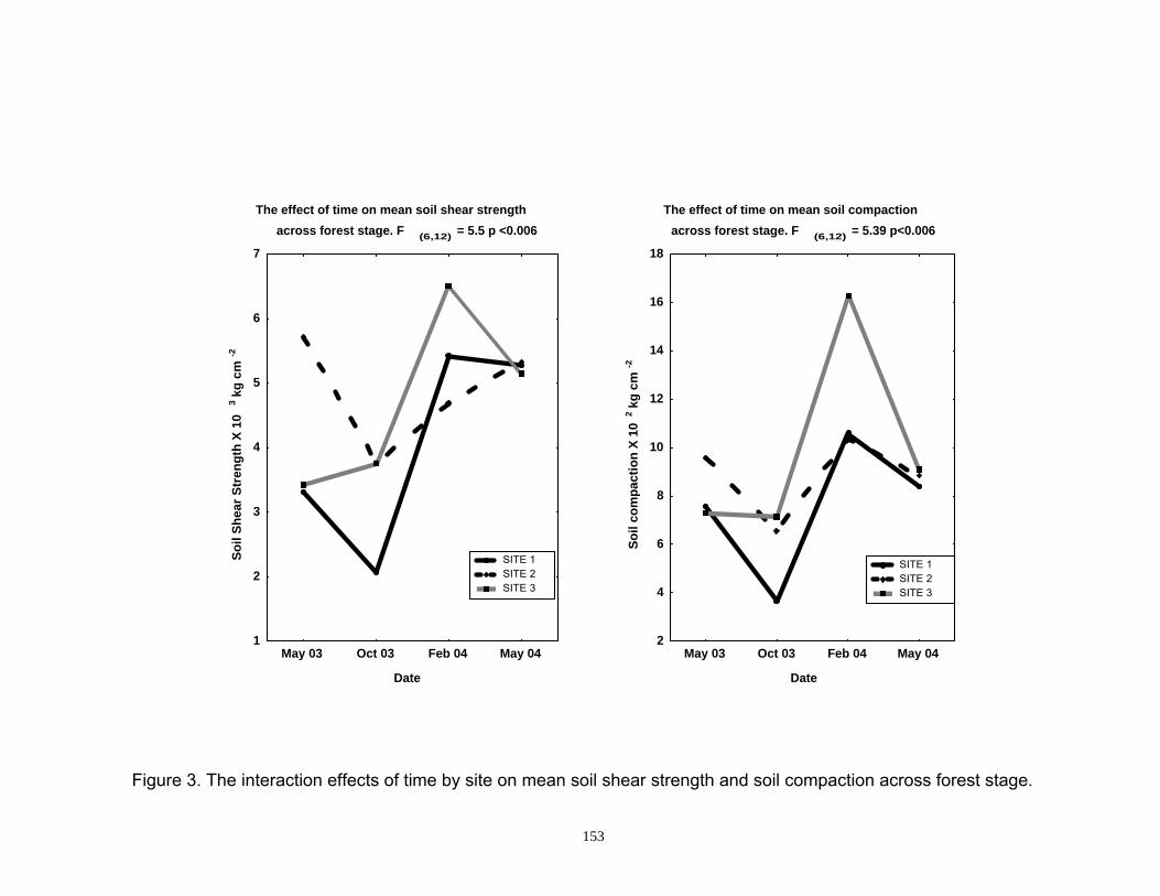
The effect of time on mean soil shear strengthacross forest stage. F (6,12) = 5.5 p <0.006

Date

Soil

Shea

r Str

engt

h X

103 k

g cm

-2

1

2

3

4

5

6

7

May 03 Oct 03 Feb 04 May 04

SITE 1 SITE 2 SITE 3

The effect of time on mean soil compactionacross forest stage. F (6,12) = 5.39 p<0.006

Date

Soil

com

pact

ion

X 10

2 kg

cm-2

2

4

6

8

10

12

14

16

18

May 03 Oct 03 Feb 04 May 04

SITE 1 SITE 2 SITE 3

Figure 3. The interaction effects of time by site on mean soil shear strength and soil compaction across forest stage.

153

New gap 1

21.0018.5014.509.504.00

Ele

vatio

n (m

m) M

ean

+- 1

SE

20

0

-20

-40

-60

-80

Forest 1

21.0018.5014.509.504.00

20

0

-20

-40

-60

-80

Recovering gap 1

21.0018.5014.509.504.00

20

0

-20

-40

-60

-80

New gap 2

21.0018.5014.509.504.00

Ele

vatio

n (m

m) M

ean

+- 1

SE

20

10

0

-10

-20

Forest 2

21.0018.5014.509.504.00

20

10

0

-10

-20

Recovering gap 2

21.0018.5014.509.504.00

20

10

0

-10

-20

New gap 3

Months since strike

21.0018.5014.509.504.00

Ele

vatio

n (m

m) M

ean

+- 1

SE

20

10

0

-10

-20

Forest 3

Months since strike

21.0018.5014.509.504.00

20

10

0

-10

-20

Recovering gap 3

Months since stirke

21.0018.5014.509.504.00

20

10

0

-10

-20

Figure 4. The absolute soil surface elevation (mean ± 1 SE) for the three forest stages (New, recovering, forest) at three sites (1,2,3). Accretion dotted line, Original soil surface solid line, surface elevation of Shallow-RSET dashed line, surface elevation of entire soil profile dot dash line (Deep-RSET).

154

Chapter V

Groundwater control of mangrove surface elevation: shrink-swell varies with soil depth.

Abstract

I measured monthly soil surface elevation change and determined its

relationship to groundwater changes at a mangrove forest site along the Shark

River, Everglades National Park, Florida. I combined the use of an original-

design surface elevation table with new rod-surface elevation tables to separately

track changes in the mid zone (0-400 cm), the shallow root zone (0-35 cm), and

the full sediment profile (0-600 cm), respectively, in response to site hydrology

(daily river stage, and daily groundwater piezometric pressure). In addition, we

calculated expansion/contraction for each of the four constituent soil zones

(surface [accretion/erosion; above 0 m], shallow zone [0-0.35 m], middle zone

[0.35-4 m], and bottom zone [4-6 m]) that comprise the entire soil column.

Changes in groundwater pressure correlated strongly with changes in soil

elevation for the entire profile (Adj. R2 = 0.90); however, this relationship was not

proportional to the depth of the soil profile sampled. The change in thickness of

the bottom soil zone accounted for the majority (R2 = 0.63) of the entire soil

profile expansion and contraction. The influence of hydrology on specific soil

zones and absolute elevation change must be considered when evaluating the

impact of disturbances, sea level rise, and water management decisions on

coastal wetland systems.

155

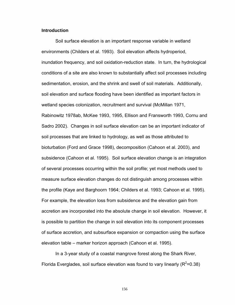
Introduction

Soil surface elevation is an important response variable in wetland

environments (Childers et al. 1993). Soil elevation affects hydroperiod,

inundation frequency, and soil oxidation-reduction state. In turn, the hydrological

conditions of a site are also known to substantially affect soil processes including

sedimentation, erosion, and the shrink and swell of soil materials. Additionally,

soil elevation and surface flooding have been identified as important factors in

wetland species colonization, recruitment and survival (McMillan 1971,

Rabinowitz 1978ab, McKee 1993, 1995, Ellison and Fransworth 1993, Cornu and

Sadro 2002). Changes in soil surface elevation can be an important indicator of

soil processes that are linked to hydrology, as well as those attributed to

bioturbation (Ford and Grace 1998), decomposition (Cahoon et al. 2003), and

subsidence (Cahoon et al. 1995). Soil surface elevation change is an integration

of several processes occurring within the soil profile; yet most methods used to

measure surface elevation changes do not distinguish among processes within

the profile (Kaye and Barghoorn 1964; Childers et al. 1993; Cahoon et al. 1995).

For example, the elevation loss from subsidence and the elevation gain from

accretion are incorporated into the absolute change in soil elevation. However, it

is possible to partition the change in soil elevation into its component processes

of surface accretion, and subsurface expansion or compaction using the surface

elevation table – marker horizon approach (Cahoon et al. 1995).

In a 3-year study of a coastal mangrove forest along the Shark River,

Florida Everglades, soil surface elevation was found to vary linearly (R2=0.38)

156

with surface water stage 15 to 30 days prior to sampling (Smith and Cahoon

2003). The investigation was limited in that the benchmarks used to measure

soil elevation extended just 4 m into the soil and stopped approximately 2 m

above the limestone bedrock. Consequently, processes occurring below the 4 m

deep benchmark were not included in the elevation readings. Additionally, the

influence of processes within the active root zone (e.g., root

growth/decomposition or shrink/swell) on soil elevation could not be determined

because the benchmarks integrated processes over the entire 4 m soil column.

Because of these limitations we added sampling devices, which allowed us to

measure the shallow active root zone (0-0.35 m) and the deeper soil zone (4-6

m).

I present here a study of soil elevation dynamics in the lower Shark River

drainage that extends over the entire soil profile and distinguishes between three

depths within the soil profile; the 0-0.35 m, 0-4 m, and 0-6 m. My main objective

was to investigate the relationship among changes in soil surface elevation and

changes in the hydrological parameters of river stage and groundwater

piezometric head pressure at the site over the three depths. Additionally, we

wanted to determine the relative contribution to soil elevation by each of the four

components of the soil profile: surface (i.e., accretion), shallow zone (active root

zone; 0 – 0.35 m), middle zone (0.35 – 4 m), and bottom zone (4 – 6 m).

A comprehensive understanding of the influences of hydrology on the soil

profile at this site is of considerable importance. The site is located in the Shark

River estuary, downstream of the Shark River Slough, and receives freshwater

157

inputs from the greater Everglades drainage and thus is under the influence of

upstream water management practices of the Greater Everglades. The

Everglades drainage is currently undergoing an ecosystem restoration

concentrating on modifying water deliveries to mimic pre-drainage flows. In

addition to the changing freshwater flows linked to restoration, this mangrove

forest is impacted by sea level rise. Determining how hydrology influences the

specific soil zones and surface elevation will allow managers to make more

informed decisions regarding these two opposing hydrological processes.

Materials and Methods

SET theory

The Surface Elevation Table (SET), based on the design of Boumans and

Day (1993), allows for precise measurements of soil surface elevation (± 1.4 mm

total error; Cahoon et al. 2002a). The SET consists of a mechanical arm that is

attached to a benchmark and leveled, establishing a fixed measuring point.

Typically each SET has four fixed measurement locations (directions), where

nine measuring pins are lowered to the soil surface to obtain a relative soil

elevation. The elevation is the mean of 36 measuring pin readings per

benchmark. SETs have been successfully used to monitor changes in elevation

in a number of wetland environments (Cahoon et al.1999). They have been used

to monitor mangrove vertical accretion and subsidence (Cahoon and Lynch

1997) and to follow the response of soil elevation to season (Childers et al.

1993), water management (Boumans and Day 1994, Hensel et al. 1999),

158

vertebrate herbivores (Ford and Grace 1998) and hurricane disturbance (Cahoon

et al. 2003).

New SET designs have recently been described that measure the change

in soil elevation of specific parts of the soil profile (e.g. root zone, below the root

zone; Cahoon et al. 2002b). At the Shark River, the shallow-rod surface

elevation table (Shallow-RSET) benchmarks were installed to a depth that

measures elevation change in the majority of the active root zone (top 0.35 m of

the soil profile). The deep-rod surface elevation table (Deep-RSET) benchmarks

were driven to bedrock and thus measure the full soil profile. The original design

SET (Original-SET) benchmarks used by Smith and Cahoon (2003) were driven

to ~ 4 m (Fig. 1). Further information on the design and accuracy of the original

SET and RSET can be found in Cahoon et al. (2002a; b). By using a

combination of SET designs at a single study site it is possible to partition

changes in soil elevation among specific parts of the soil profile, such as the

shallow root zone and deeper soil zones (Fig. 1). By determining the absolute

change for each depth zone we can calculate expansion and contraction for each

zone (surface [accretion/erosion; above 0 cm], shallow [active root; 0-0.35 m],

middle [0.35-4 m], and bottom [4-6 m]) of the profile.

Site description

Vegetation

The study site, SH3 of Smith and Cahoon (2003), is located near the

mouth of the Shark River (Zone 17 N 2805254 mE. 0492112 mN., UTMs WGS

1984) in a mature mixed mangrove riverine forest comprised of Rhizophora

159

mangle L. (red mangrove), Laguncularia racemosa (L.) Gaertn. (white

mangrove), and Avicennia germinans (L.) Stearn (black mangrove). The site has

a sparse understory. The canopy ranges in height from 13 to 17 m. The site has

mixed tides. During the study period the Shark River had a daily average

conductivity of 40 mS cm -1 and varied between a low of 25 mS cm -1 to a high of

51 mS cm -1. Shark River discharge was greatest at the end of the wet season,

from September to November for 2002.

Soil profile

The soil profile of this site was determined from the well drilling log (G.

Anderson, unpublished, Fig 1). The mangrove peat was 5.5 m in depth. The

peat matrix lay directly on top of limestone, into which the well was drilled 1.8 m.

The transition between the peat matrix and limestone was rapid. The limestone-

peat interface was difficult to drill but had softer material below it. Otherwise, the

entire peat layer was of similar constituency. No clay deposits were encountered

during the drilling.

Cohen (1968) described the stratigraphy of the mangrove soil column at

the mouth of the Little Shark River, a location approximately 2.5 kilometers away

from SH3. He found that the mangrove peat was 3.81 m in depth and the total

depth to bedrock at the site was 3.86 m. The peat types did not have

recognizable petorgraphic constituents. All of the peat types were marine or

brackish and dominated by R. mangle. There was a general increase of fine

granular debris at the top and bottom of the profile. Fine granular debris

160

comprised approximately 35 % of the sample at the top and the bottom of the

core. At the top of the core it was suggested that an increase in fine-grained

marine carbonates were responsible for this high number. The increase in fine

granular debris at the bottom of the core may be due to greater amount of

degradation of the organic constituents of the peat. Pyrite content was relatively

high (2 % to 18%) throughout the core suggesting reducing conditions. Fusinite

only occurred at the bottom of the core and comprised a small percentage of the

constituents. There were no clays reported from this core.

Additionally, preliminary sampling of the mangrove peat hydraulic

conductivity (at a site 4 km away) yielded relatively low values (hydraulic

conductivity field saturation method (Guelph permeameter) = kfs = 1.87 m day -1,

see Hughes et al. 1998), which suggest slow water transmittance through the

surface layer of the peat (Anderson et al. 2001).

SET installation

I installed three groups of SETs within 18 m of each other and 45 m of the

Shark River. All groups were within 15 m of a United States Geological Survey

(USGS) hydrological monitoring station (USGS station # 252149081044301,

described below). Each group included one Shallow-RSET, one Original-SET,

and one Deep-RSET along with four feldspar marker horizons (Cahoon and

Turner 1989). The three Original-SETs, used in the Smith and Cahoon study

(2003), were installed on July 16, 1998. Three Shallow-RSETs and three Deep-

RSETs were installed on February 28, 2002 (Table 1). On March 18, 2002, four

161

separate layers of feldspar (0.5 - 3 mm deep) were laid as marker horizons with

each group for a total of twelve new marker horizons. Shallow-RSETs

benchmarks were installed to a depth of 0.35 m. The original-SET benchmarks

(76 mm (3”) diameter aluminum pipe (1 mm thick wall) were driven approximately

4 m deep. The Deep-RSET benchmarks (1.43 cm (9/16”) diameter stainless

steel rods) were driven to approximately 6 m deep (Table 1). All SETs and

feldspar markers were measured monthly from March 18, 2002 to March 21,

2003. Measurements were taken during low tide exposure on the same day.

Two sampling events occurred with minimal water (a few puddles) present on the

soil surface. On November 9, 2002 and on February 10, 2005 we surveyed the

elevation of only the group number 3 Shallow-RSET, Original-SET, and Deep-

RSET with standard survey methods (± 3 mm). There was no movement of the

SET devices, over this period of 2 yrs 4 mos, in relation to an established

benchmark, suggesting that the assumption of a stable datum (Childers et al.

1993, Cahoon et al. 1995, Cahoon and Lynch 1997, Cahoon et al. 2002b) was

valid during the study (Table 1).

Hydrological data

The hydrological conditions investigated were (1) daily rate of change in

groundwater piezometric pressure and (2) river stage. Groundwater head

pressure was collected from a USGS station installed at the site in 1996

(Anderson and Smith 2005, Fig. 1). A piezometer recorded groundwater head

pressure of the shallow coastal aquifer in a layer of limestone (hereafter referred

162

to as groundwater). The 7.33 m piezometer consisted of threaded 7.62 cm

diameter PVC pipe that was screened (0.20 slot PVC) from 5.7 m to 7.2 m

depth. The slotted part of the well was entirely within the limestone. The well

was sealed with “formation packer” at 5.5 m depth, the interface of the limestone

and the peat layer to prevent vertical flow. Piezometric head pressure

measurements were collected at hourly intervals. The pressure transducer was

located at the depth of the well screen (further details see Anderson and Smith

2005).

Shark River stage data were obtained from the “Shark River” hydrological

monitoring station of Everglades National Park located 2.37 km downstream from

SH3. This station records tidal influences as well as seasonal changes in river

discharge for the area. Tidal flooding occurred at the site when the Shark River

stage was above 0.07 m (Fig 2b). Shark River stage data were collected hourly.

The groundwater piezometric head pressure and the Shark River stage were

reported in North American Vertical Datum (NAVD) 88 datum (Geiod 99) (Fig 2).

Hourly Shark River stage and groundwater head pressure for the interval from

December 13, 2002 to January 9, 2003 is included in Fig. 2b and 2d. I used daily

averages of the above parameters in order to remove the diurnal tidal signal.

The daily averaged signal of these parameters shows the monthly lunar

influences on the tide (Provost 1973), annual change in sea level (Provost 1973),

and the seasonal changes in water level due to regional wet season (Fig 2a and

c). The hourly tidal signal was assumed to have minimal impact upon my SET

measurements because elevation data were always collected at low tide. Sensor

163

malfunction resulted in the loss of daily groundwater piezometric head pressure

data from October 7, 2002, to November 8, 2002, an interval that included the

October 10 SET sample measurement.

Data Analysis

Soil elevation at each SET benchmark was averaged across all measuring

pins at four directions (n=36) for each sampling event. To determine the average

daily rate of change (DRC) in the soil elevation between sampling events we

used the following formula:

Daily rate of change = average soil elevation (X t+1 – X t) / (# days in interval)

(1)

Where X t is average elevation at time t and X t+1 is the average elevation

at time t+1. The daily rates of change for all hydrological metrics were

determined in a similar fashion. For example, river stage averaged for day X t+1

was subtracted from river stage averaged for day X t and divided by the number

of days in the interval. The daily average hydrological metrics were used in the

analysis to remove hourly tidal effects (Fig. 2).

Within the three SET types, we used forward stepwise multiple regression

to investigate the relationship between daily rate of change in soil elevation for

each of the three benchmarks and the rates of change in the hydrological

parameters and accretion. Stepwise multiple linear regression was used to

164

discern the most important hydrologic variables associated with incremental

elevation change. Stepwise regression not only allows for the identification of the

most parsimonious model, but accounts for correlation among two or more

variables (Zar 1999). All parameters included in the models were tested for

collinearity and normality of the residuals (Quinn and Keough 2002). All models

were analyzed using STATISTICA 5.0 (Statsoft, Inc., 1996) and SPSS 11.0

(SPSS, Inc., 2001). The final models included the two hydrological parameters:

(1) daily rate of change in groundwater piezometric pressure, and (2) daily rate of

change in river stage. Within each SET type, we used a data set reduced from

36 data intervals (12 monthly intervals X 3 benchmarks) to 30 data intervals as a

result of the hydrological data gap for groundwater piezometric pressure.

Because there was only one well at the site, the hydrologic data was used three

times, once for each SET type analysis. This may call into question the

independence of the hydrology well data. I felt justified in presenting the

hydrologic data with individual SET data for two reasons: 1) to emphasis small

scale spatial variation in soil surface elevation; 2) we had no reason to expect

hydrological variation over this small distance mainly due to consistency in the

soil matrix.

I felt that regression using interval rate of change (as opposed to a

regression of cumulative change) was justified because the focus of the study

was to discover the relationship between elevation change and hydrologic

variable from one sampling interval to the next. Furthermore, interval data

should reduce the influence of any serial correlation. Due to the length of time

165

between samples (monthly intervals), we felt that there was little influence of prior

values on the relationships within a given interval. Regressions between the

interval rate of change of soil elevation and the interval rate of change of

hydrologic variables have been used previously (Childers et al. 1993).

By using the absolute change for each benchmark depth sampled by the

three types of SET (Shallow-RSET, Original-SET, and Deep-RSET) we could

calculate expansion and contraction for each component of the soil profile using

the following formula.

Entire profile expansion/contraction = Accretion + (Shallow-RSET – Accretion) +

(Original-SET – Shallow-RSET) + (Deep-RSET – Original-SET).

(2)

Thickness of the entire soil profile is equal to the sum of surface accretion (above

0 m), and changes in thickness of the active root zone (0-0.35 cm), the middle

zone (0.35 - 4 m), and the bottom zone (4-6 m).

Results

Site hydrology

Both seasonal and monthly lunar influences were important for the

hydrological conditions at the site (Fig. 2). The highest monthly mean stages at

the Shark River were in September and October (-0.23 and –0.19 m

respectively), typical for this drainage. The high river stage was a result of the

maximum discharge of accumulated water from the wet season (June to

166

September, Fig. 2). Groundwater piezometric head pressure was also high

during September and October (0.06 and 0.12 m respectively) due to

hydrological recharge from the wet season. Daily river stage was a reflection of

monthly lunar tidal flooding, wet season river discharge and annual sea level

variability (thermal expansion, Provost 1973).

There was moderate correlation between the two hydrological metrics

used in the multiple regression with an r = 0.72 for Shark River stage to

groundwater piezometric head pressure. Tolerance values were above 0.547

and Variance Inflation Factors were less than 1.829, suggesting that despite

some correlation between predictor variables, collinearity was not a serious issue

for these data (Quinn and Keough 2002; Neter et al. 1996).

Accretion

The feldspar marker horizons did not become completely covered until

172 days after installation (September 10, 2002). The marker horizons were

covered with mineral, organic and root matter. The annual accretion rate was

6.64 ± 0.56 mm yr-1 (± 1 SE). Sediment deposition values were intermittent in

nature with high rates in October 2002 and March 2003 (Fig. 3a). Slight erosion

was evident during the November to December 2002 period (-1.8 mm) and the

December 2002 to January 2003 (-0.8 mm) sampling.

167

Soil elevation

Changes in absolute soil surface elevation for both the Deep-rod and

Original- SETs followed a similar pattern (Fig. 3c and d). Both devices recorded

the highest mean soil elevations at the end of the wet season (8.89 mm on

October 10, 2002 for the Original-SET and 15.14 mm on November 9, 2002 for

the Deep-RSET) and the lowest mean elevations during the dry season (January

09, 2003; -2.24 mm and -0.06 mm respectively). The Shallow-RSETs had a

distinctly different pattern of soil surface elevation, with the highest elevation at

the end of the wet season (6.83 mm on November 9, 2002) and the lowest early

in the wet season (-0.66 mm on June 03, 2002, Fig. 3b).

Relationships between soil elevation and hydrology

The daily rate of soil elevation change of the Shallow-RSET was partially

explained (Adjusted R2 = 0.16) by a negative relationship with the daily rate of

change of the river stage at the site (Table 2). That is, as river stage increased,

the soil elevation that was influenced by the shallow soil zone decreased (Fig.

4a). The rate of soil elevation change of the Original SET was positively related

with the daily rate of change of the groundwater head pressure (Adjusted R2 =

0.61; Fig. 4b; Table 2). This model was run with a reduced data set (n=28) due

to a one time sampling error of Original SET 2. The daily rate of change of soil

elevation for the Deep-RSET had a strong positive relationship to the daily rate of

change of the groundwater head pressure (Adjusted R2 = 0.90; Fig. 4c; Table 2).

168

When groundwater head pressure increased the soil elevation increased for both

the Original SET and the Deep-RSET.

Contribution of each zone to expansion/contraction of the entire profile

I calculated the variation in thickness of each of the four constituent soil

zones (Eq. 2) and for the entire soil profile. I determined how much each of

these soil zones contributed to absolute change of the entire profile by using a

stepwise multiple regression model in which absolute change in the thickness of

the entire profile was the dependent variable and the absolute change in

thickness for each soil zone were independent variables.

The contribution of each soil zone was not equivalent to the relative

proportion of soil profile it comprised (Fig. 5). The bottom zone (4-6 m)

accounted for 63% of the variation in the absolute change in thickness of the

complete profile whereas the middle zone (0.35 – 4 m) accounted for only 22%

(Table 3, Fig. 5). However, the bottom zone comprises only 31% of the entire

profile whereas the middle zone comprises 63%. Accretion and the shallow zone

were not significant contributors to the overall absolute change in thickness of the

entire profile (Table 3).

Discussion

The soil surface elevation changed substantially during the year; the

Deep-RSETs recorded the greatest average elevation (15.14 mm) at the end of

the wet season (November 09, 2002). The patterns of cumulative change in soil

169

surface elevation were very similar for both the Deep-RSET and Original-SET,

but the pattern of the Shallow-RSET was distinctly different (Fig. 3). The overall

annual accretion rate of 6.6 mm yr-1 was similar to the 4.4 to 7.8 mm yr-1 reported

in another mangrove study in SW Florida (Cahoon and Lynch 1997). The

influence of accretion and/or erosion on the change in soil elevation was minimal

over the duration of this study, as it was not a significant factor in any of the

regression models. Furthermore, elevation for all three SETs had changed

substantially before accretion at the site was even measurable, indicating the

importance of subsurface processes. In addition to accretion and soil swelling,

shallow and deep subsidence have been reported to be significant factors for the

interpretation of soil elevation change (Cahoon et al 1995). Here we were able to

account for the opposing influences of subsidence and soil swelling by sampling

the entire soil profile while including deposition/erosion in multiple regression

models.

Subsurface hydrological processes and soil elevation change

The entire mangrove peat-dominated soil profile was strongly influenced

by groundwater. The rate of change in groundwater head pressure had a strong

positive linear relationship to the rate of change in soil surface elevation for the

Deep-RSET (Adj. R2=0.90), suggesting that the entire soil profile is swelling in

response to hydrological recharge. In this area, change in the daily groundwater

piezometric pressure reflects freshwater recharging of the estuary and monthly

tidal influences. Other mangrove SET researchers (e.g., Cahoon and Lynch

170

1997; Smith and Cahoon 2003) have reported seasonal response to soil

elevation. However, a direct relation to forcing by a hydrological parameter has

not been previously shown. Because this particular peat has relatively low

superficial hydrological conductivity and is typically continuously saturated, peat

swelling may not be the only mechanism explaining this relationship.

Nevertheless the tight coupling suggests this is the most likely mechanism

driving changes in soil elevation.

Soil shrink-swell has been reported numerous times but almost exclusively

in regards to soils with high clay compositions (Hillel 1971). As far as the

author’s are aware there are few reported shrink-swell observations in regards to

wetland soils composed almost exclusively of peats driven by changes in

groundwater head pressure. Those studies reported are confined to Sphagnum

peatlands (Price and Schlotzhauer 1999) along with one reference to surface

elevation changes in a saltmarsh, but this was linked to semidiurnal surface tidal

flooding (Nuttle et al. 1990). My study indicates that changing groundwater head

pressure was driving the monthly shrink-swell of the soil surface elevation in this

peat matrix. Another study (Cahoon and Lynch 1997) suggested the importance

of mangrove peat shrink and swell, in addition to growth/decomposition and

shallow subsidence as possible mechanisms for explaining annual elevation

patterns. In my study, we were able to show that the peat matrix undergoes

shrink and swell and that the majority of the expansion/contraction occurs in the

bottom zone.

171

The shallow soil zone

Soil elevation over the depth of the root zone had a moderate relationship

with the daily rate of change in Shark River daily stage (adjusted R2 = 0.16). The

first five sampling events recorded no deposition since marker horizons were not

completely covered; yet we recorded substantial change in surface elevation

influenced by the shallow soil zone suggesting belowground influences. It should

be noted that the marker horizons showed progression towards complete

coverage by having less of the marker horizon visible each of the five successive

sampling events. I were able to remove the influence of deposition and erosion

by determining the relationship between thickness of the shallow zone (0-35cm)

and river stage. As daily rate of change for the river stage increased, the

thickness of the shallow active root zone decreased (R2 = 0.24, F (1,34) = 10.57 p

<0.004). This analysis indicates that changing river stage has a stronger

influence than previously noted for elevation change; however, it is still only a

moderate relationship. The lack of a strong hydrological link to the shallow soil

profile is not wholly unexpected. Biological (root growth, crab burrow dynamics)

processes rather than strictly hydrological influences dominate this shallow soil

zone. Other possible explanations for the lack of a strong hydrological coupling

are a shift in redox to more reducing conditions, or a decline in root growth.

Erosion and deposition were not a great influence in explaining the

change in surface elevation of the Shallow-RSET over the short period of this

study for the following reasons: 1) The rate of deposition/erosion was not a

significant parameter in the Shallow-RSET model; 2) the first five sampling

172

events indicate substantial change in surface elevation influenced by the shallow

soil zone when no deposition / erosion was measured; 3) the model was rerun for

only those periods with marker horizons measurements and no difference was

found in the final model.

Cumulative proportion of profile sampled and the role of the bottom zone.

The response of the soil elevation change does not appear to be directly

proportional to the depth of the soil profile encompassed by the SET device. The

Original-SET (0-4m) followed the groundwater influence (R2 = 0.61), but not as

strongly as the Deep-RSET (0-6 m; R2 = 0.90). Compared to the Deep-RSET,

the Original-SETs encompassed 2 m less of the soil profile, which reduced the

coupling between change in soil elevation and change in groundwater

piezometric pressure (slope of the regression equation ß1 = 0.040 for the

Original-SET vs. ß1 = 0.074 for the Deep-RSET, Table 2).

I used the proportion of the soil profile sampled by the Original-SET as

compared to the Deep-RSET to predict the average elevation of the Original-SET

based on the corresponding Deep-RSET readings. For example, Original-SET

number one benchmark depth was 4.04 m and the Deep-RSET number one

benchmark depth was 5.47 m, resulting in a proportion of the entire soil profile

sampled by Original-SET number one of 0.74 (i.e., 4.04 / 5.47 m). If the

relationship was linear with proportion of soil profile sampled then the actual

values should fall near the calculated values along the one to one line (Fig. 6).

The values predicted for Original-SET based on this ratio were higher than the

173

actual elevation values recorded (Fig. 6), suggesting that the deepest 2 m of peat

not encompassed by the Original-SET have a disproportionately larger influence

on the absolute soil elevation.

To further corroborate the importance of the influence of the bottom zone

on overall soil profile expansion and contraction; we determined the percent of

variation explained by each component zone to overall soil column expansion

and contraction. I determined that the largest constituent zones, the middle and

bottom zones drive the expansion and contraction of the entire profile. These

two parts account for 94.2 % of the soil profile and explain 85 % of the variance

in overall soil profile expansion and contraction. However, the bottom zone

accounted for 63% of the variation in the absolute change in thickness but

comprised only 31% of the profile. The middle zone accounted for only 22% of

the variation but comprised 63% of the profile (Table 3; Fig. 5). These data

suggest that the bottom zone has a greater influence on overall change in soil

surface elevation than would be expected based on its relative proportion and

that in this zone changing ground water pressure would be the most influential.

My results indicate that increases in groundwater flow should have a direct

positive impact on absolute soil surface elevation for the entire soil profile by

expanding the bottom soil zone. Since expansion and contraction affects the

water storage potential of the peat matrix it is an important consideration for

studies of water balance, and nutrient fluxes (Nuttle et al. 1990). The current

hydrological restoration of the Everglades and increases in sea level will directly

affect this mangrove forest. Any modification to freshwater flows via the

174

Everglades Restoration will affect the elevation of the mangrove forest by

expansion and/or shrinkage. In order to determine how other processes

(bioturbation, organic production, decomposition, disturbance, and subsidence)

will affect long-term change in soil surface elevation, researchers must account

for this shrink and swell signal and remove it from the analysis. The influence of

these hydrological processes must be taken into account in the context of

monitoring the effects of hydrological restoration or sea level rise. Understanding

the factors influencing the change in soil elevation as it relates to different parts

of the soil profile will be critical when trying to predict long-term mangrove

sustainability in an increasing sea level environment.

175

Acknowledgments

This work was supported by the Global Climate Change Program of the

United States Geological Survey / Biological Resources Discipline and the United

States Department of Interior’s “Critical Ecosystems Studies Initiative”

administered by Everglades National Park under Interagency agreement

#IA5280-7-9023. Sampling occurred under Everglades National Park permit

EVER-2002-SCI-0029 and EVER-2003-SCI-0056. I thank C. Walker and H.

Barreras for field assistance and P. Hensel and C. Husby for statistical

consultation. Assistance with manuscript editing from S. F. Oberbauer, C. A.

Ugarte, R. M. Price, D. M. Lee, M. McClain, D. Childers, and the Ecosystem

Review Group along with helpful insight from two anonymous reviewers are

gratefully appreciated. Mention of trade names does not constitute endorsement

by the US Government.

176

Literature Cited Anderson, G.H., T.J. Smith III, and T.M. Lavin 2001. Variation in mangrove peat

hydrologic conductivity across the riparian mangrove forest near the Harney River, Everglades National Park: Preliminary observations. International Estuarine Research Federation biannual meeting St. Petersburg, Florida. pp. 6 November 4-8, 2001.

Anderson, G.H., and T.J. Smith III. 2005. The Mangrove Hydrology Sampling

Network in Everglades National Park: Hypotheses, Network Design and Data for the Lower Shark River for Water Years 1996 - 2002. U.S. Geological Survey, Open-File Report OFR02-457. Saint Petersburg, Florida.

Boumans, R., and J.W. Day, Jr. 1993. High precision measurements of soil

elevation in shallow coastal areas using a sedimentation-erosion table. Estuaries 16: 375-380.

Boumans, R., and J.W. Day, Jr. 1994. Effects of two Louisiana marsh

management plans on water and materials flux and short-term sedimentation. Wetlands 14: 247-261.

Cahoon, D.R., and R.E. Turner. 1989. Accretion and canal impacts in a rapidly

subsiding wetland II. Feldspar marker horizon techniques. Estuaries 12:260-268.

Cahoon, D.R., D.J. Reed, and J.W. Day, Jr. 1995. Estimating shallow subsidence

in microtidal salt marshes of the southeastern United States: Kaye and Barghoorn revisited. Marine Geology 128:1-9.

Cahoon, D.R., and J.C. Lynch. 1997. Vertical accretion and shallow subsidence

in a mangrove forest of southwestern Florida, U.S.A. Mangroves and Salt Marshes 1:173-186.

Cahoon, D.R., J. Day, and D. Reed. 1999. The influence of surface and shallow

subsurface soil processes on wetland elevation: a synthesis. Current Topics in Wetland Biogeochemistry 3:72-88.

Cahoon, D.R., J.C. Lynch, P. Hensel, R. Boumans, B.C. Perez, B. Segura, and

J.W. Day, Jr. 2002a. A device for high precision measurement of wetland sediment elevation: I. Recent improvements to the sedimentation-erosion table. Journal of Sedimentary Research 72:730-733.

177

Cahoon, D.R., J.C. Lynch, B.C. Perez, B. Segura, R. Holland, C. Stelly, G. Stephenson, and P. Hensel. 2002b. A device for high precision measurement of wetland sediment elevation: II. The rod surface elevation table. Journal of Sedimentary Research 72:734-739.

Cahoon, D.R., P.R. Hensel, J. Rybczyk, McKee, K.L., E.E. Proffitt, and B.C.

Perez. 2003. Mass tree mortality leads to mangrove peat collapse at Bay Islands, Honduras after Hurricane Mitch. Journal of Ecology 91:1093-1105.

Childers, D.L., F.H. Sklar, B. Drake, and T. Jordan. 1993. Seasonal

measurements of sediment elevation in three Mid-Atlantic estuaries. Journal of Coastal Research 9:986-1003.

Cohen, A.D. 1968. The Petrology of some peats of Southern Florida (with special

reference to the origin of Coals). Ph.D. Dissertation, The Pennsylvania State University. Pennsylvania. Vol. 1 part 1, pp. 332-334.

Cornu, C.E. and S. Sadro. 2002. Physical and functional responses to

experimental marsh surface elevation manipulation in Coos Bay’s South Slough. Restoration Ecology 10: 474-486.

Ellison, A.M., and E.J. Farnsworth. 1993. Seedling survivorship, growth, and

response to distrubance in Belizean mangal. American Journal of Botany 80 :1137-1145.

Ford, M.A., and J.B. Grace. 1998. Effects of vertebrate herbivores on soil

processes, plant biomass, litter accumulation and soil elevation changes in a coastal marsh. Journal of Ecology 86:974-982.

Hensel, P.R., J.W. Day, Jr., and D. Pont. 1999. Wetland vertical accretion and

soil elevation change in the Rhone River delta, France: the importance of riverine flooding. Journal of Coastal Research 15:668-681.

Hillel, D. 1971. Soil and water physical principles and processes. Physicological

ecology, A series of monographs, texts and treatises. Academic press, Inc; New York, USA.

Hughes, C.E., P.Binning, and G.R. Willgoose. 1998. Characterisation of the

hydrology of an estuarine wetland. Journal of Hydrology 211:34-49. Kaye, C.A., and E.S. Barghoorn. 1964. Late Quaternary sea-level change and

crustal rise at Boston, Massachusetts, with notes on the autocompaction of peat. Geological Society of America Bulletin 75:63-80.

178

McKee, K.L., 1993. Soil physicochemical patterns and mangrove species distribution-reciprocal effects? Journal of Ecology 81:477-487.

McKee, K.L., 1995. Seedling recruitment patterns in a Belizean mangrove forest: effects of establishment ability and physico-chemical factors. Oecologia 101:448-460.

McMillan, C., 1971. Environmental factors affecting seedling establishment of the

black mangrove on the central Texas coast. Ecology 52:927-930. Neter, J., M.H. Kutner, C.J. Nachtsheim, and W. Wasserman. 1996. Applied

linear regression models. 3rd edition Irwin publishing, Chicago, IL. USA. Provost, M.W. 1973. Mean high water mark and use of tidelands in Florida.

Florida Scientist 1:50-66. Quinn, G.P., and M.J. Keough. 2002. Experimental design and data analysis for

biologists. 1st edition. Cambridge University press, United Kingdom. Rabinowitz, D., 1978a. Dispersal properties of mangrove propagules. Biotropica

10:47-57. Rabinowitz, D., 1978b. Early growth of mangrove seedlings in Panama, and a

hypothesis concerning the relationship of dispersal and zonation. u 5:113-133.

Smith, T.J. III, and D.R. Cahoon. 2003. Wetland sediment elevation in the Florida

Everglades: response to surface water stage variation, Proceedings of the International Conference on Coastal Sediments 2003. May 18-23, 2003, Clearwater Beach, FL, USA. CD-ROM Published by World Scientific Publishing Corp. and East Meets West Productions, Corpus Christi, Texas, USA. ISBN 981-238-422-7.

Statsoft, Inc 1996 Statisitca for Windows, Tulsa, OK. Statsoft, INC. SPSS, Inc 2001 SPSS for Windows 11.0.1 Zar, J.H. 1999. Biostatistical analysis. Fourth edition Prentince Hall; New

Jersey, USA. SOURCES OF UNPUBLISHED MATERIALS Anderson, G.H. unpublished data. U.S. Geological Survey, Well drilling log for SH3 Hydrological Station, records maintained at Everglades National Park Field Station, 40001 State Rd 9336, Homestead, FL., USA 33034.

179

Table 1. Depth of benchmark (m) for each SET and dates of establishment. Elevations for Group 3 SETs (mm) only with the first elevation on November 02, 2002 and second elevation on February 10, 2005 (NAVD 88 Geido 99).

Device

Establishment Date

Group

1

Group

2

Group

3

First

Elevation

Second

Elevation

Shallow-RSET

February 28, 2002

0.35 0.35 0.35 338 338

Original-SET

July16, 1998

4.04 4.09 4.32 405 405

Deep-RSET

February 28, 2002

5.47 6.08 6.57 131 131

180

Table 2. Regression equations and statistical results for daily rate of change (DRC) of surface elevation and DRC of best-fit hydrological parameters for the three SET types used in this study.

Y (dependent variable)

m (slope)

x (independent variable)

b (intercept) N P F df

Adj. R2

DRC Shallow-RSET -0.012 DRC River Stage 0.08 3.69 2,27 0.16 30 0.0383DRC Original-SET 0.040 DRC Groundwater head pressure -0.068 42.35 1,26 0.61 28 0.0001DRC-Deep-RSET 0.074 DRC Groundwater head pressure -0.067 259.7 1,28 0.90 30 0.0001

Table 3. Linear regression equations and statistical results for the absolute change in thickness of entire profile and the absolute change of each of the constituent components. Stepwise regression with p <.01 to enter and p < .9 to exit model. Overall model R2 = 0.85.

Y (dependent variable)

m (slope)

x (independent variable)

b (intercept) t P

Proportion of R2

Proportion of soil profile

1.74 2.349 0.025 Change in thickness of entire profile Middle zone 0.812 6.843 0.0001 .22 .63

Bottom Zone 1.197 13.340 0.0001 .63 .31 Surface (Accretion) n.s. < .01 Shallow zone n.s. .06

181

Figure 1. Profile of the substrate showing Original, Deep, and Shallow-RSETs, groundwater well and relative depth of each benchmark at Shark River mangrove site. (Adapted from Cahoon et al. 2002b with permission of the author). Drawing at 1:24 scale.

182

Figure 2. Hydrograph of (A) Daily averaged Shark River stage, (B) Hourly Shark River stage interval from December 13, 2002 to January 9, 2003, (C) Daily averaged groundwater piezometric head pressure and (D) Hourly groundwater

183

M A M J J A S O N D J F M A

-4

-2

0

2

4

6

8

10

12

14

16

18

20

mm (±1 SE

)

Accretion

M A M J J A S O N D J F M A

-4

-2

0

2

4

6

8

10

12

14

16

18

20

mm (±1 SE

)

Shallow RSET

M A M J J A S O N D J F M A

-4

-2

0

2

4

6

8

10

12

14

16

18

20

mm (±1 SE

)

Original SET

M A M J J A S O N D J F M A

-4

-2

0

2

4

6

8

10

12

14

16

18

20

mm (±1 SE

)

Deep RSET

2002 2003

D

C

B

A

Figure 3. Mean absolute soil surface elevation (±1SD) for (A) Accretion, (B) Shallow-RSET, (C) Original-SET, and (D) Deep-RSET.

184

A M J J A S O N D J F M A-0.5

-0.4

-0.3

-0.2

-0.1

0.0

0.1

0.2

0.3

0.4

0.5

-10

-8

-6

-4

-2

0

2

4

6

8

10

Ele

vatio

n C

hang

e (m

m/d

ay)

Deep RSET

2002 2003

Gro

undw

ater

Cha

nge

(mm

/day

)

Groundwater

C

A M J J A S O N D J F M A-0.5

-0.4

-0.3

-0.2

-0.1

0.0

0.1

0.2

0.3

0.4

0.5

-10

-8

-6

-4

-2

0

2

4

6

8

10

Ele

vatio

n C

hang

e (m

m/d

ay)

Original SET

2002 2003

Gro

undw

ater

Cha

nge

(mm

/day

)

Groundwater

A M J J A S O N D J F M A-0.20

-0.15

-0.10

-0.05

0.00

0.05

0.10

0.15

0.20

-10

-8

-6

-4

-2

0

2

4

6

8

10

Ele

vatio

n C

hang

e (m

m/d

ay)

Shallow RSET

2002 2003

Riv

er S

tage

Cha

nge

(mm

/day

)

River Stage

B

A Figure 4. Mean (±1SD) rate of change for the three Shallow-RSETs and the rate of change in river stage (A), three Original-SETs and rate of change in groundwater piezometric head (B), and three Deep-RSETs and rate of change in groundwater piezometric head (C).

185

186

A M J J A S O N D J F M A-10

-5

0

5

10

15

20

Cha

nge in Thick

ness

(mm±1

SE)

Shallow Zone

A M J J A S O N D J F M A-10

-5

0

5

10

15

20

Cha

nge in Thick

ness

(mm±1

SE)

Middle Zone

A M J J A S O N D J F M A-10

-5

0

5

10

15

20

Cha

nge in T

hick

ness

(mm±1

SE)

Bottom Zone

2002 2003

A M J J A S O N D J F M A-10

-8

-6

-4

-2

0

2

4

6

8

10

12

14

16

18

20

Cha

nge in T

hick

ness

(mm±1

SE)

Entire ProfileA

B

C

D

Figure 5. Mean (±1SD) Absolute change in thickness of the (A) entire profile, (B) shallow zone, (C) middle zone, and (D) bottom zone.

Calculated soil surface elevation (mm)

Act

ual s

oil s

urfa

ce e

leva

tion

(mm

)

-5

0

5

10

15

-5 0 5 10 15

Original-SET1Original-SET2Original-SET3

Figure 6. Actual soil surface elevation of the Original SET (mm) versus calculated soil surface elevation (mm) (proportion of the Deep-RSET). Dark solid line represents 1:1 ratio. n = 36.

187

Chapter VI

Conclusion

Lightning-initiated canopy gaps are an important but relatively

understudied disturbance in mangrove forests around the world and are

particularly important in the mangrove forests of Everglades National Park. I

found that the environmental conditions within the gaps differed from the

surrounding forest. The expanded gap size averaged 289 ± 20 m2 ( ± SE). As

gaps filled with saplings, light transmittance decreased exponentially. Overall,

gaps had greater fine woody debris but less coarse woody debris than the

surrounding forest. Soil torsion and soil compaction were lower in the gaps than

the forest. The abundance of fiddler crab burrows decreased with distance

upstream, additionally large and medium burrow abundance increased linearly

with total seedling abundance. Newly formed lightning gaps had greater dead

root biomass compared to the intact forest. I did not find a systematic reduction

in the soil cohesiveness as new gaps aged. Soil surface elevation declined

between 8.5 mm to 60.9 mm in newly formed lightning gaps; this loss was due to

superficial erosion (8.5 mm) and subsidence (60.9mm). Lightning apparently kills

many of the shallow surface roots and leads to a decline in the soil surface

elevation in new gaps. Subsidence occurring below the shallow soil zone

generated the greatest overall soil elevation loss. Recovering (Growing) gaps

had lower live root biomass but similar soil surface elevation patterns as the

intact forest. This study suggests that if Rhizophora mangle can exploit the

188

increased flooding from soil surface elevation loss in new lightning strike gaps,

then it would have to occur in the first 7 to 10 years. After this time, the soil

surface elevation patterns (recovering gap) reflect the intact forest eventually

removing this opportunity. I was unable to find a relationship between the

change in soil elevation and survivorship, mortality rate, or recruitment in the new

gaps. However, because of the small sample size (n = 3 new gaps) and the

short time period of the study, this is not a unexpected result.

I found that the saplings and seedlings in new gaps survived the lightning

strike, and this is the first documented evidence that in a mangrove forest a large

amount of the non-canopy trees present before the lightning strike survive. This

evidence comes in the form of a distinct two-cohort regeneration apparent in the

seedling and sapling height distribution. The first cohort consists of the

propagules and seedlings present at the site pre-strike and individuals recruiting

very soon after the canopy is removed. The second group recruits into the site

some number of years post strike. The high densities of Rhizophora mangle as

seedlings and saplings in the recruiting and growing gaps stages imply that

lightning strike disturbances in these mangroves favors their recruitment and

does not favor Avicennia germinans and Laguncularia racemosa. However,

average A. germinans seedling height was found to increase in later gap stages,

suggesting an increase in the transition probability from seedling to sapling stage

perhaps related to gap successional development.

Enumerating survival, recruitment, and growth across life stages by

species is of critical importance in understanding and predicting changes in forest

189

structure, composition, and development especially in mangrove communities.

This dissertation is the first report of recruitment/mortality rates for multiple

mangrove species across life stages in gaps and closed canopy forest. Survival,

recruitment, and growth varied across three successional stages of mangrove

forest (newly initiated lightning gaps, closing gaps, and intact forest). The life

stage parameters for the three dominate life phases (seedlings, saplings, and

adult) of the three dominant mangroves (Avicennia germinans, Laguncularia

racemosa, Rhizophora mangle) differed.

The seedling and sapling recruitment rates of A. germinans were 1.5 times

greater than mortality in new lighting-initiated canopy gaps indicating an

expanding population. New gaps also had 2.6 to 10.6 times greater rate of

seedling mortality for R. mangle and L. racemosa compared to the recruitment

rate, indicating decreases in these populations. Seedling stem elongation was

greatest in the new gaps. Taken together at least, seedling recruitment rate

during my study was twice as high in new gaps, as in the other forest stages.

Presumably this recruitment rate will continue to increase as the conditions within

the gaps favor propagules establishment. Additionally, I conclude that new light

gaps may favor A. germinans seedling recruitment in this initial stage of gap

succession. Finally, future studies of life stage population parameters (survival,

recruitment, and growth) should include recruiting gaps. From the extremely high

densities of R. mangle seedlings and saplings in the study it must concluded that

R. mangle recruitment and survivorship increase greatly some time after the new

gap stage of succession.

190

At the growing gap stage of development seedling mortality rate of R.

mangle was 10 times greater and sapling mortality was 13 times greater than

recruitment. The recruitment of R. mangle adults was 4 times greater than

mortality. The gaps have developed to a phase in which there was reduced stem

elongation, sapling and adult growth, and few individuals able to recruit into the

adult life stage. Sapling populations are high (~ 1 sapling m2), and seedling

populations are low (0.6 seedling m2). R. mangle dominates seedling and

sapling stages of the growing gaps and eventually are making the transition to

the adult life stage. The end results indicate that at the growing gap stage of

succession of the lightning gaps R. mangle stems were being favored as adult

trees.

In the intact forest, A. germinans seedlings and sapling recruitment was 3

times greater than the mortality rate. Additionally, L. racemosa and R. mangle

seedling mortality was 2 times greater than the recruitment and sapling mortality

was 28 times greater than recruitment. In general, growth within the forest was

low across all life stages compared to the new gaps. These population

parameter results suggest that A. germinans becomes a co-dominant to

dominant in closed canopy mangrove forest of South Florida (Craighead 1971)

by having higher recruitment than mortality for the seedling and sapling stages.

Given enough time the population of A. germianans seedlings and saplings will

continue to expand whereas the populations of L. racemosa and R. mangle were

decreasing.

191

In conclusion, this study suggest that lightning strike disturbance in these

mangroves favors R. mangle recruitment based on densities and does not favor

A. germinans and L. racemosa. Overall, vegetative dynamics in lightning

initiated canopy gaps indicate that this disturbance may maintain South Florida

mangroves in a cyclical or arrested successional state of development. My

results provide population parameters needed to understand and predict

recruitment and survivorship for each of the three dominant species (A.

germinans, L. racemosa, and R. mangle) during the gap-phase dynamics of the

mangrove forest and within the intact closed canopy forest. Additionally, I

determined growth estimates enabling better understanding of intact forest and

development within the stages of gap-phase dynamics. The results of this study

provide new insights into the regeneration process of lightning disturbed systems

and into other mangroves systems experiencing gap dynamics mechanisms.

Potential impact of Everglades Restoration on lightning gap dynamics.

I was able to show that site hydrology (both as groundwater head

pressure and river stage) does have a direct impact on the soil elevation both in

the intact forest (both short-term (Chapter V) and long-term (Chapter IV)) and in

disturbed sites. However, I was unable to make a strong link to seedling

recruitment or survival to changes in soil elevation. I found that a number of the

environmental variables that varied with river location: amount of coarse woody

debris, soil bulk density, soil torsion and soil compaction and fiddler crab (Uca

thayeri) burrow densities. Additionally, river location was significant for

192

propagule and seedling densities in R. mangle, propagules of L. racemosa, and

biomass of L. racemosa and R. mangle. However, I believe that the long-term

gap successional trajectory will be minimally impacted by Everglades

hydrological restoration. The gap dynamics appear to have a consistent pattern

regardless of river position. R. mangle dominates seedlings in recruiting gaps

and saplings in the growing gaps at all of the sites along the river. Additionally,

R. mangle seedlings, saplings, and adults in this forest are highly resilient to

hydrological conditions (Krauss 2004). The unknown variable is the influence of

hydrological manipulation on A. germinans and L. racemosa recruitment.

However, since it appears that R. mangle is favored by lightning gap disturbance

on the whole river, the impact of manipulated hydrology will be minimal on the

gap successional process. The rate at which the gap transitions between forest

successional stages may be affected by changes in hydrological discharge,

however, and determination of changes in transition rates will have to be the

subject of future studies. Sea level rise is also impacting this forest. In the short-

term ecological view, the Everglades restoration will clearly influence the

hydrology the mangrove forests even affecting the soil elevation. However, sea

level rise will continue to modify the mangrove community by driving

transgression into the freshwater marshes beyond the ability of management to

mitigate the long-term impacts.

193

Literature Cited

Craighead, F.C. 1971. The Trees of South Florida. Vol. I. The Natural Environments and Their Succession. University of Miami Press, Miami, FL, USA.

Krauss, K.W. 2004. Growth, photosynthetic and water use characteristics of

South Florida mangrove vegetation in response to varying hydroperiod. Ph.D. dissertation University of Louisiana, Lafayette, Louisiana, USA.

194

VITA

KEVIN RICHARD TERRENCE WHELAN

1993 B.Sc., Biological Sciences, Florida International University, Magna Cum Laude, Minor in Chemistry 1997 M.Sc., Biological Sciences, Florida International University, Thesis: Short Term Response of Two Cypress Communities (Taxodium distichum var. imbricarium (Nuttall) Croom) within Everglades National Park to the Effects of Hurricane Andrew. 2001-2005 Student Career Experience Program appointment Ecologist United States Geological Survey Florida Integrated Science Center Center for Coastal and Watershed Studies 2001 - 2002 Research Biologist II, Johnson Controls 1998 - 2001 Research Biologist II, AScI Corporation 1997- 1997 Research Biologist, Southeast Environmental Research Program Florida International University 1993 –1996 Graduate Research Associate and Project Manager Biological Sciences Department Florida International University PUBLICATIONS AND PRESENTATIONS Krauss, K.W., T.W. Doyle, R.R. Twilley, T.J.Smith III, K.R.T. Whelan, and J.K.

Sullivan. 2005. Woody debris in the mangrove forests of South Florida. Biotropica 37:9-15.

Oberbauer, S.F., von Kleist III, K., Whelan, K.R.T., and Koptur, S. 1996. Effects

of Hurricane Andrew on epiphyte communities within cypress domes of Everglades National Park. Ecology, 77(3), 964-967.

Whelan, K.R.T., and T.J. Smith III. 2004. Lightning Gaps in the Mangroves

Forest of Everglades National Park. U.S. Geological Survey Fact Sheet, FS 2004-3016

195

Whelan, K. R.T., and T.J. Smith III 2002. Annual Permit Report #EVER-2002-SCI-0029 Study # EVER-00132. Small gap dynamics in the mangroves of Everglades National Park and South Florida.

Whelan, K.R.T., T.J. Smith III, D.R. Cahoon, J.C. Lynch, and G. H. Anderson,

2004. Groundwater changes influence sediment elevation in a mangrove forest along the Shark River, Florida. First National Conference on Ecosystem Restoration. Lake Buena Vista, Florida.

Whelan, K.R.T., and T.J. Smith III. 2004. Root mortality in recent lightning-

formed canopy gaps of a Neotropical mangrove forest leads to soil elevation loss. The Association of Tropical Biology. Miami, Florida.

Whelan, K.R.T., and T.J. Smith III. 2003. Characteristics of lightning gaps in the

mangrove forests of south Florida. Estuarine Research Federation 17th Biennial International Conference. Seattle, Washington.

Whelan, K.R.T., J.H. Waddle, T.J. Smith III, and K.G. Rice. 2003. Stratification

of Hylids within a mangrove habitat of South Florida. Joint meeting of Ichthyologists and Herpetologists. Manaus, Amazonas, Brazil.

Whelan, K.R.T., T.J. Smith III, D.R. Cahoon, and J.C. Lynch. 2003. Short term

changes in sediment elevation of a mangrove forest. Society of Wetland Scientists 24 th annual meeting. New Orleans, Louisiana.

Whelan, K.R.T., and T.J. Smith III. 2003. Characteristics of lightning gaps in the

mangrove forest of Everglades National Park. Greater Everglades Ecological Research (GEER) Science Conference. Naples, Florida.

Whelan, K.R.T., T.J. Smith III, and I. van Leth. 2002. Lightning gap

characteristics in the mangroves of south Florida. The Ecological Society of America 87th annual meeting. Tucson, Arizona.

Waddle J.H., K.R.T. Whelan, K.G. Rice, and T.J. Smith III. 2001. Anuran

Dynamics in Fringing Riverine Mangrove Habitat. Estuarine Research Federation 16th Biennial International Conference.

Whelan, K.R.T., and T.J. Smith III. 2000. Seedling Dynamics Across a

Mangrove - Sawgrass Ecotone in the Southwest Florida Everglades. Greater Everglades Ecosystem Restoration (GEER) Science Conference. Naples, Florida.

196