flow estimation

8/7/2019 Flow Estimation

http://slidepdf.com/reader/full/flow-estimation 1/9

Fast Panoramic Image Mosaicing UsingOne-dimensional Flow Estimation

In this paper, we propose a fast method for panoramic image mosaicing using one-dimensional (1D) flow estimation. First, the 1D flow vectors are estimated at each pixel in xand y directions. Then the global affine parameters are estimated from 1D flows using the

iterative least-squares method. The accurate parameters are obtained by iteratively repeated

optimization in x and y directions. We have implemented the proposed method on a conventionallow-cost PC. The experimental results show that the image mosaicing is possible in near-real time.

# 2002 Elsevier Science Ltd. All rights reserved.

Junichi Hoshino1 and Masakatsu Kourogi2

1College of Engineering Systems, University of Tsukuba,

1-1-1 Tennoudai, Tsukuba,

Ibaraki 305-8573, Japan2National Institute of Advanced Industrial Science and Technology,

1-1-1 Umezono, Tsukuba,

Ibaraki 305-8568, Japan

Introduction

Panoramic image mosaicing is a useful technique for

many applications such as virtual reality, video surveil-

lance, and aerial image analysis [1 – 10]. One of the

problems of panoramic image mosaicing is that its

computational cost is so high that the image processing

required usually cannot be done in real time by a low-

cost PC.

Real-time performance is important for applica-

tions such as video surveillance because we need to see

current situations. However, it often takes more than

several seconds to calculate transform coefficients

between images. For example, an optimization tech-

nique such as the Levenberg–Marquadt method

[3,4] requires an accurate initial estimation of the

coefficients, and more than a few hundred iterations to

converge. It takes nearly a minute using standard

implementations.

In this paper, we propose a fast method for

panoramic image mosaicing using 1D flow estimation.

First, the approximate motion vectors x and y directions

are estimated. Then the global affine parameters are

estimated using the least-squares method. The accurate

parameters are obtained by iteratively repeated optimi-

zation in x and y directions.

We have implemented the proposed method on a

conventional low-cost PC. The experimental results

show that the accuracy of the image mosaicing

is comparable to the existing methods, and

achieves 10–100 times faster performances traditional

methods.

1077-2014/02/$35.00 r 2002 Elsevier Science Ltd. All rights reserved.

Real-Time Imaging 8, 95–103 (2002)

doi:10.1006/rtim.2001.0257, available online at http://www.idealibrary.com on



Previous works

One of the conventional methods is a cylindrical

panorama which covers a horizontal view [6]. This

method limits the camera motion around the horizontal

axis of the optical center, and forces users to carry a

tripod. The other typical approach of making image

mosaicing is to estimate the transform coefficients

between images such as affine transform or perspective

transform. For example, Szeliski created panoramic

images by minimizing the sum of the squared intensity

errors using the Leverberg–Marquadt method [3,4]. This

type of non-linear optimization technique requires a

good initial estimate (e.g. x and y translation compo-

nents) which is often computationally expensive. For

example, the popular method described in [3] applies the

correlation-based matching within the whole image. It

takes more than several seconds only to estimate the

initial translation component. In addition, the Leven-berg–Marquadt method needs more than a few hundred

iterations to converge. It sometimes takes nearly a

minute for computation.

Some methods extract image features such as corners,

and estimate transform coefficients by feature matching

[7–9]. However, the feature extraction and matching is

often computationally expensive. The feature matching

process is complex because some features which appear

in one frame can disappear in the other frames. Someresearchers focus on the shorter processing time using

the feature-based matching [9]. However, it still takes

10 s to overlay 2 images.

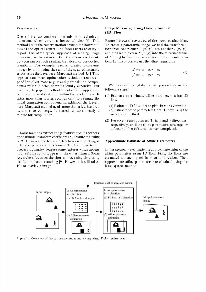
Image Mosaicing Using One-dimensional(1D) Flow

Figure 1 shows the overview of the proposed algorithm.

To create a panoramic image, we find the transforma-

tion from one picture I 0 (x0

i

; y0

j

) into another I (xi , yi ),

and then warp picture I 0 (x0i ; y0

j ) into the reference frame

of I (xi , yi ) by using the parameters of that transforma-

tion. In this paper, we use the affine transform.

x0 ¼a1x þ a2 y þ a3

y0 ¼a4x þ a5 y þ a6

ð1Þ

We estimate the global affine parameters in the

following steps:

(1) Estimate approximate affine parameters using 1D

flow.

(a) Estimate 1D flow at each pixel in x or y direction.

(b) Estimate affine parameters from 1D flow using the

last squares method.

(2) Iteratively repeat process (1) in x and y directions,

respectively, until the affine parameters converge, or

a fixed number of steps has been completed.

Approximate Estimate of Affine Parameters

In this section, we estimate the approximate value of the

affine parameters using 1D flow. First, 1D flows areestimated at each pixel in x or y direction. Then

approximate affine parameters are obtained using the

least-squares method.

Figure 1. Overview of the panoramic image mosaicing using 1D flow estimation.

96 J. HOSHINO AND M. KOUROGI



1D flow estimation

Let the displacements in x and y directions be (vx,v y).

The error between a background I (xi , yi) and an input

image I 0 (x0i ; y0

j ) is

I ðxi þ vx; yi þ v yÞ À I 0ðx0i ; y0

i Þ

¼ I ðxi ; yi Þ þ vx

@

@xI ðxi ; yi Þ þ v y

@

@ yI ðxi ; yi Þ À I 0ðx0

i ; y0i Þ

ð2Þ

Let @I (xi , yi )/@x be I x, and @I (xi , yi )/@ y be I y. I x and I y

can be obtained by using the finite difference scheme (i.e.I x ¼ I ðxi ; y j Þ À I ðxi þ1; y j Þ; I y ¼ I ðxi ; y j Þ À I ðxi ; y j þ1Þ).

By substituting I t ¼ I ðxi ; yi Þ À I 0ðx0i ; y0

j Þ into Eqn. (4),

we obtain

I xvx þ I yv y þ I t ¼ 0 ð3Þ

This is the well-known optical flow constraint

equation [17,18]. We cannot solve Eqn (4) because

we have only one equation for the two motion

parameters. The conventional optical flow methods

introduce constraints to estimate motion parameters in

two dimensions [17,18]. However, such constraints

typically cause the increase in computational costs

(Figure 2).

Instead of introducing additional constraints, we

approximately estimate the optical flow in one dimen-

sion to reduce computational costs. For example, if we

estimate the 1D flow in x direction

rx ¼ ðÀI t=I x; 0Þ ð4Þ

Also, we obtain the 1D flow in y direction

r y ¼ ð0; ÀI t=I yÞ ð5Þ

We use these 1D flows at each pixel to estimate affine

parameters. These 1D flows are quite noisy in general.

However, we can increase the accuracy of the estimationusing the iterative least-squares method described in the

next section.

Affine parameter estimation

In the next step, the global affine parameters are

estimated from the 1D motion vectors. Given a motion

vector (vx, v y) and a threshold th, the motion vectors can

be selected by testing the following condition [19]:

jI ðx; yÞ À I 0ðx þ vx; y þ v yÞjoth ð6Þ

Since the true motion vector should satisfy this

equation, it is possible to verify the 1D motion vectors

by testing this condition. We use a threshold th=10 for

experiments. The regions are not empirically selected

when Eqn. (6) is applied. Eqn. (6) is computed at all the

points in the image. Only 1D flow vectors within the

overlapped regions are used for affine parameter

estimation.

Then, we obtain affine parameters using the least-

squares method [16]. Let Ax ¼ ½a1; a2; a3�T; A y ¼

½a4; a5; a6�T and ¼ ½1; x; y�T. Then Eqn. (1) can beexpressed as

vxðx; yÞ ¼ TAx; v yðx; yÞ ¼ TA y ð7Þ

The affine parameters Ax and A y can be estimated as

follows:

Ax ¼X

Th iÀ1 X

½vxðx; yÞ�

A y ¼

XT

h iÀ1

X½v yðx; yÞ�

ð8Þ

Iterative Update of Affine Parameters

The affine parameters estimated in the previous section

are not accurate because of errors in 1D flow estimation.

In this section, we increase the accuracy of the affine

parameters by iteratively repeating the optimization in x

and y directions.

x-coordinate

Intensity

v x

I t

Slope = I x

Figure 2. Approximate estimate of vectors; ( ) I (xi , yi );( ) I 0ðx0

i ; y0i Þ.

FAST PANORAMIC IMAGE MOSAICING 97



The process of the iterative estimation can be

summarized as follows.

(1) When t ¼ 0 (t represents the number of iterations),

we obtain the initial estimate of affine parameters A0

using the method described in the previous section.

(2) When t ! 1, the affine parameters are updated usingAtÀ1 ¼ fa1; . . . ; a6g. First, new 1D flows are

estimated:

rx 0

¼ðÀI t=I x þ x0i ; y0

i Þ

r y 0

¼ðx0i ; ÀI t=I y þ y0

i Þð9Þ

where ðx0i ; y0

i Þ is

x0i ¼a1xi þ a2 yi þ a3

y0i ¼a4xi þ a5 yi þ a6

ð10Þ

I t can be obtained as follows:

I t ¼ I ðx; yÞ À I 0ðx þ x0i ; y þ y0

i Þ ð11Þ

Then, we estimate new affine parameters from frx0

i g

or fr y0

i g using the least-squares method as described

earlier.

(3) Repeat (2) in x and y directions, respectively, until

the affine parameters converge, or repeat the fixed

number of iterations.

Experiments

The proposed method is implemented using a conven-

tional PC (CPU: PentiumII-400 MHz, RAM 128M, OS:

Linux-2.0). We show the following experimental results

to demonstrate the effectiveness of the proposed method.

Convergence process and statistics

We present a simple case of panoramic image mosaicing

to show the typical behavior of the proposed method.

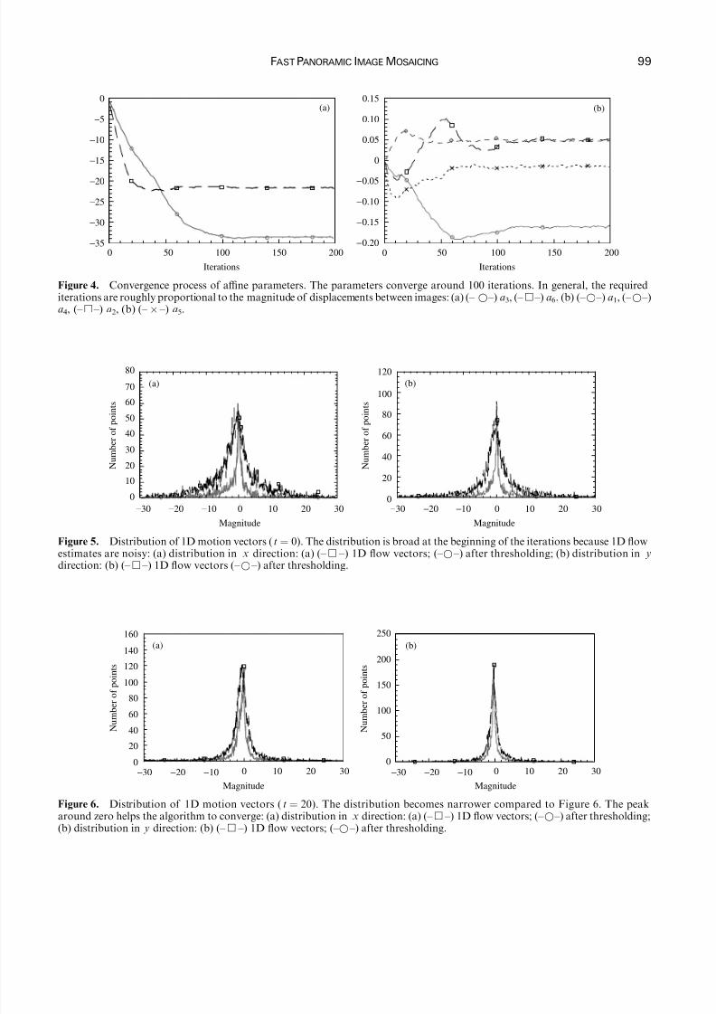
Figure 3(a) and (b) are input images. Figure 4 shows the

convergence process of affine parameters. Figure 3(c) isthe result of merging two pictures with the affine

parameters fa1; . . . ; a6g ¼ ð À0.160, 0.046, À33.925,

0.047, À0.017, À21.802). Figures 5 and 6 show the

Figure 3. Experimental results using 2 pictures: (a) input image 1; (b) input image 2; (c) overlapping (a) (b).




0

20

40

60

80

100

N u m b e r o f p o i n t s

120

0

10

20

30

40

50

60

70

−30 −20 −10 0 10 20 30


80

Magnitude

−30 −20 −10 0 10 20 30

Magnitude

(a) (b)

Figure 5. Distribution of 1D motion vectors (t ¼ 0). The distribution is broad at the beginning of the iterations because 1D flowestimates are noisy: (a) distribution in x direction: (a) (– & –) 1D flow vectors; (– * –) after thresholding; (b) distribution in ydirection: (b) (– & –) 1D flow vectors (– * –) after thresholding.

0

50

100

150

200

−30 −20 −10 0 10 20 30

N u m b

e r o f p o i n t s

250

Magnitude

0

20

40

60

80

100

120

140

−30 −20 −10 0 10 20 30

N u m b

e r o f p o i n t s

160

Magnitude

(b)(a)

Figure 6. Distribution of 1D motion vectors (t ¼ 20). The distribution becomes narrower compared to Figure 6. The peakaround zero helps the algorithm to converge: (a) distribution in x direction: (a) (– & –) 1D flow vectors; (– * –) after thresholding;(b) distribution in y direction: (b) (– & –) 1D flow vectors; (– * –) after thresholding.

−35

−30

−25

−20

−15

−10

−5

0

0 50 100 150 200−0.20

−0.15

−0.10

−0.05

0

0.05

0.10

0.15

Iterations

0 50 100 150 200

Iterations

(a) (b)

Figure 4. Convergence process of affine parameters. The parameters converge around 100 iterations. In general, the requirediterations are roughly proportional to the magnitude of displacements between images: (a) (– * –) a3, (– & –) a6. (b) (– * –) a1, (– * –)a4, (– & –) a2, (b) (– Â –) a5.




distribution of 1D flow at the different stages of the

iterations, where (a) shows the component of

rx ¼ ðÀI t; =I x; 0Þ, and (b) shows the y component of

r y ¼ ð0; ÀI t; =I yÞ. We can see that the distribution is

slightly biased to the translational direction. This

characteristic contributes the algorithm to converge to

the true estimates. Tables 1 and 2 show the statistics of

the distributions. (V x, V y) denote the original 1D flow,

and (V 0x; V 0 y) the 1D flow after thresholding. For thereference, the statistics of the normal distribution is

skewness=0 and kurtosis=3. We can observe that the

flow vectors are biased to the true estimates. The

averages of the distribution correspond to the magni-

tude of translational shift during one iteration. The

positive value of the skewness means the distribution

leans toward the left (negative x and y directions).

Comparison with the normal flow estimation

In this paper, we use 1D flow in x and y directions toestimate global affine parameters. The other possible 1D

flow is the normal flow [10–15] which has been used to

Table 1. Statistics of 1D motion vectors (t ¼ 0). The distribu-tion is broad at the beginning of the iterations, and biasedtoward the true estimates

Average Variance Skewness Kurtosis

V x À0.1878 51.917 0.3571 7.9761

V y À0.0148 64.929 0.0655 7.8291V 0x À0.4853 23.157 0.9545 11.984V 0 y À0.4005 31.333 0.1276 12.172

Table 2. Statistics of 1D motion vectors (t ¼ 20). Thedistribution becomes narrower. The peak around zero helpsthe algorithm to converge well

Average Variance Skewness Kurtosis

V x À0.0041 5.6971 0.1003 84.030

V y À0.1391 5.1348 0.1770 36.914V 0x À0.0536 1.4255 12.647 433.48V 0 y À0.0593 2.0544 2.448 46.570

0

50

100

150

200

−30 −20 −10 0 10 20 30


250

Magnitude

0

50

100

150

200

−30 −20 −10 0 10 20 30


250

Magnitude

(a) (b)

Figure 7. Distribution of normal flow vectors (t ¼ 0): (a) distribution in x direction: (a) (– & –) 1D flow vectors; (– * –) afterthresholding; (b) distribution in y direction: (b) (– & –) 1D flow vectors; (– * –) after thresholding.

−25

−20

−15

−10

−5

0

0 50 100 150 200 250 300

Iterations

0 50 100 150 200 250 300

Iterations

−0.08

−0.06

−0.04

−0.020

0.02

0.04

0.06

0.08(a) (b)

Figure 8. Convergence process of affine parameters using normal flow: (a) (– * –) a3, (– & –) a6; (b) (– * –) a1, (– ̂ –) a4, (– & –) a2,(b) (– Â –) a5.




estimate global camera motion. Use of the normal flow

for the image mosaicing has not been presented in

previous papers. However, the comparison may beinteresting because the normal flow has been the typical

method of generating 1D flow.

Normal flow is a 1D flow along the gradient direction.

The magnitude of the normal flow is

jvnj ¼ I t= ffiffiffiffiffiffiffiffiffiffiffiffiffiffiffi

I 2x þ I 2 y

q ð12Þ

Figure 9. Panoramic image mosaicing from a continuous video sequence.

−7

−6

−5

−4

−3

−2

−1

0

0 5 10 15 20 25

Iterations

−0.02

−0.01

0

0.01

0.02

0.03

0 5 10 15 20 25

Iterations

(a) (b)

Figure 10. Convergence process of affine parameters when the inter-frame motion is small. The parameters converge faster thanthe example of Figure 4: (a) (– * –) a3, (– & –) a6; (b) (– * –) a1, (– * –) a4, (– & –) a2, (b) (– Â –) a5.

Table 3. Computation time.

Affine parameter estimation 30–40 msImage gradient 10 msID flow vectors 10 msLeast-squares estimation 10 ms

Image merging 10 msTotal 40–50 ms

0

20

40

60

80

100

−30 −20 −10 0 10 20 30

Magnitude


120

Figure 11. Distribution of 1D flow at different thresholds.Threshold value is not so sensitive because it maintains similardistribution characteristics: (F) no threshold; (F)th=10;(F)th=20; (??????)th=5.




where gradient direction n is

n ¼1 ffiffiffiffiffiffiffiffiffiffiffiffiffiffiffi

I 2x þ I 2 y

q ðI x; I yÞT ð13Þ

From Eqns. (12) and ( 13), x and y components of the

normal flow are given as

ðvx; v yÞ ¼ ÀI tI x

I 2x þ I 2 y

; ÀI tI y

I 2x þ I 2 y

!ð14Þ

Figures 7 and 8 show the results of the affine

parameter estimation using the normal flow. The results

show that convergence process is quite slow compared

with the 1D flows described previously. In this experi-

ment, the affine parameters did not converge even after

300 iterations.

Merging continuous video sequences

Figure 9 shows the result of panoramic image mosaicing

from continuously captured video images (80 frames).

Figure 10 shows the convergence process of affine

parameters. Table 3 shows the computational time of

the same sample. In this example, the affine parameters

converge around 10 iterations because the inter-frame

motion is much smaller compared with the example

above. The computational cost of the proposed method

is roughly O(tMN ) where t is the number of iterations

and (M ,N ) is the size of the input images. In the current

implementation, the proposed method can process l0–20

frames per second using continuously captured video

sequences (Figures 11 and 12).

Conclusion

In this paper, we proposed a fast method for panoramic

image mosaicing using 1D flow estimation. The algo-

rithm converges very well without introducing any

additional constraints. The accuracy of the image

mosaicing is comparable to the existing method even if

we use the approximate flow estimates. We also show

that the proposed method converges quickly compared

with the estimation using the normal flow. The

experimental results show that the image mosaicing is

possible from continuously captured video sequences in

near-real time. In future, we plan to extend the proposed

method to merge input images including outliers such as

moving objects.

References

1. Brown, L.G. (1992) A Survey of image registrationtechniques. ACM Computer Surveys 24: 325–376.

Figure 12. Flow distribution of the different input images. We can observe similar results for the typical input images: (a) inputimage 1; (b) input image 2; (c) flow distribution of input image 1; (d) flow distribution of input image 2.


flow estimation

Documents