flow in unsatruated random porus media, nonlinear...

Flow in unsaturated random porous media,nonlinear numerical analysis and comparison to

analytical stochastic models

Thomas Hartera,* & T.C. Jim Yeh b

aHydrology Program; University of California, Davis, Parlier, CA 93648, USAbDepartment of Hydrology and Water Resources; the University of Arizona, Tucson, AZ85719, USA

(Received 20 May 1997; revised 15 December 1997; accepted 26 March 1998)

This work presents a rigorous numerical validation of analytical stochastic models ofsteady state unsaturated flow in heterogeneous porous media. It also provides a cruciallink between stochastic theory based on simplifying assumptions and empirical fieldand simulation evidence of variably saturated flow in actual or realistic hypotheticalheterogeneous porous media. Statistical properties of unsaturated hydraulic con-ductivity, soil water tension, and soil water flux in heterogeneous soils are investigatedthrough high resolution Monte Carlo simulations of a wide range of steady state flowproblems in a quasi-unbounded domain. In agreement with assumptions in analyticalstochastic models of unsaturated flow, hydraulic conductivity and soil water tensionare found to be lognormally and normally distributed, respectively. In contrast,simulations indicate that in moderate to strong variable conductivity fields,longitudinal flux is highly skewed. Transverse flux distributions are leptokurtic. themoments of the probability distributions obtained from Monte Carlo simulations arecompared to modified first-order analytical models. Under moderate to strongheterogeneous soil flux conditions (j2

y $ 1), analytical solutions overestimatevariability in soil water tension by up to 40% as soil heterogeneity increases, andunderestimate variability of both flux components by up to a factor 5.Theoretically predicted model (cross-)covariance agree well with the numericalsample (cross-)covarianaces. Statistical moments are shown to be consistent withobserved physical characteristics of unsaturated flow in heterogeneous soils.q 1998Elsevier Science Limited. All rights reserved

Keywords:soil water, vadose zone, stochastic analysis, heterogeneity, flow modeling.

1 INTRODUCTION

Groundwater recharge, irrigation efficiency, runoff, evapo-transpiration, and transport of contaminants, vapors, andsolutes in the vadose zone are examples of the diverse andimportant issues associated with a good understanding ofunsaturated flow processes and their spatial variability.Spatial variability of soil texture, saturated and unsaturatedhydraulic conductivity, moisture content, and water tensionin the unsaturated zone have been reported over the past twodecades in numerous field studies. These studies found thatthe permeability of soils may vary by orders of magnitude

over very short distances (decimeters to meters). Variabilityin soil moisture content and soil tension is significant withcoefficients of variation from less than 10% to more than50%17,18.

To investigate the effect of spatial variability on watermovement in the unsaturated zone several stochastic ana-lyses of unsaturated flow problems have been conducted inthe past. Using analytical methods, Yeh et al.53–56 andMantoglou and Gelhar29–31have found that the anisotropyof effective unsaturated hydraulic conductivity is moisturedependent and hysteretic, and that the variability of soil–water pressure and moisture content increases as soils dryout. These findings are consistent with observations oflateral interflow to streams and rivers60, extensive lateral

Advances in Water ResourcesVol. 22, No. 3, pp. 257–272, 1998q 1998 Elsevier Science Ltd

Printed in Great Britain. All rights reserved0309-1708/98/$ - see front matterPII: S 0 3 0 9 - 1 7 0 8 ( 9 8 ) 0 0 0 1 0 - 4

257

*Corresponding author.

migration of contaminants7–9,52 and complex hillslopehydrological processes33. Similar analytical approacheshave been developed to investigate migration of contami-nants in the unsaturated zone44,45. While these analyseshave advanced our understanding of the effect of hetero-geneity and furnished means for estimating effectiveparameters and variability of soil water flow, they areknown to be strictly applicable only to soils with lowvariability due to first-order approximations and implicitnormality assumptions in the derivation of these analyticalmodels.

More recently, Monte Carlo simulations of unsaturatedflow have been applied to avoid some of the limitations ofanalytical stochastic models. Hopmans et al.26 investigatedsoil water tension distribution in a shallow unsaturated zonewith multiple, stochastically separate soil horizons. Yeh56

examined the effective hydraulic conductivity in layeredsoils. Soil water flux variability in a one-dimensional flowdomain and the dependence of variability on boundary con-ditions were the focus of work by U¨ nlu et al.46. Other studiesdescribe the physical dynamics of soil water flow in indi-vidual, numerically generated, hypothetical soil profileexamples1,38,41,43. Because of numerical difficulties mostof these studies have been limited to soils with a varianceof the unsaturated hydraulic conductivity up to one(j2

y # 1,y¼ logK, whereK is unsaturated hydraulic conduc-tivity, log refers to natural logarithm). In contrast, fieldmeasurements indicate thatj2

y is often as high as 3, some-times even higher2,6,28,50,37,48.

The purpose of this work is to provide a general, com-prehensive numerical validation of existing analyticalstochastic models for steady state unsaturated flow under arealistic range of soil conditions including high spatialvariability, varying degrees of statistical anisotropy, andboth dry and wet soil conditions. We illustrate the relation-ship between abstract stochastic models and physical obser-vations of unsaturated flow in heterogeneous soils tounderline the significance of stochastic models in our under-standing of soil water dynamics. To alleviate the numericalproblems associated with computing soil water flow underconditions of large variability and to reduce overall compu-tational requirements, we use a recently developed efficientnumerical approach for the simulation of steady stateunsaturated flow in heterogeneous soils21. Here, theapproach is expanded for the implementation of highresolution Monte Carlo simulations with a large numberof realizations. The specific objectives of this paper are todetermine and prove the statistical sampling accuracy of theMonte Carlo simulations, to derive joint probability distri-butions associated with soil–water pressure head, unsatu-rated hydraulic conductivity, and soil water flux in deepunsaturated soils, to compare their means, variances, and(cross-)correlation functions with those obtained from ana-lytical models, and to link observations of soil waterdynamics in individual soil profiles with the statisticalresults derived here. The study provides important informa-tion regarding the validity and limitations of simplified

assumptions commonly employed in stochastic analysis offlow in unsaturated porous media.

2 METHODOLOGY

Steady state flow in two-dimensional porous media undervariably saturated conditions is governed by Richardsequation25:

]

]xiKi(h)

](xz þ h)]xi

� �¼ 0 i ¼ x,z, (1)

wherexx andxz are the horizontal and vertical coordinates,respectively.xz is positive upward,h is the matric potentialor pressure head (negative for unsaturated conditions).Einstein summation is implied. Specific flux in thexi direc-tion is given by Darcy’s law:

qi ¼ ¹ Ki(h)](hþ xz)

]xi: (2)

In this study, the exponential conductivity model firstuggested by Gardner14 is used to describe unsaturatedhydraulic conductivity,K, as a function of matric potential,h,

K(h) ¼ Ksexp(ah), (3)

wherea is a pore-size distribution parameter,Ks is satu-rated hydraulic conductivity, assumed to be locally iso-tropic. In agreement with field studies,Ks and a areassumed to be random space functions (RSFs) with log-normal distributions49. The RSFs logKs, log a, log K, h,andq are expanded to

logKs(x) ¼ f ¼ F(x) þ f 9(x) (4)

loga(x) ¼ a¼ A(x) þ a9(x)

logK(x) ¼ y¼ Y(x) þ y9(x)

h(x) ¼ H(x) þ h0(x)

qi(x) ¼ Qi(x) þ q9i(x),

where F(x), A(x), Y(x), H(x) and Qi(x) are the expectedvalues of logKs(x), log a (x), log K(x), h(x) and qi(x),respectively, andf9(x), a9(x), y9(x), h9(x), and q9 i (x) arezero-mean, second-order stationary perturbations at loca-tion x. We define the geometric mean ofa by G, whereG ; exp (A).

The numerical flow model, MMOC2, used in this studyand its integration into Monte Carlo simulation is fullydescribed by Harter22 and Yeh et al.57. The numericalmodel is based on the Galerkin finite element techniqueusing rectangular elements and bilinear shape-functions.The nonlinearity in the flow problem is solved iterativelyusing a Newton–Raphson scheme and an incomplete LUpreconditioned conjugate gradient method. After matricpotentials are found from eqn (1) with state eqn (3),MMOC2 solves Darcy’s eqn (2) with a Galerkin finite

258 T. Harter, T. C. Jim Yeh

element method to guarantee a continuous flux field,q(x),throughout the domain. A semi-analytical, first-orderspectral solutionhL is used as initial guess of the steadystate solution to reduce the computational cost of solvingRichards eqn (1) numerically. A complete description andvalidation of this method is given by Harter and Yeh21.

To simulate gravity drainage in deep soils with a watertable beyond the reach of the simulation domain, and toaccount for the unknown boundary conditions at the verticalboundaries of the simulation domain, random Dirichlet typeboundaries were imposed. Pressure head on all boundaries isset equal to the linearized first-order perturbation solution,hL, obtained individually for each realization off and apriori to the numerical solution. The linear solution,hL, isderived from spectral analysis and inverse Fourier trans-form. It assumes that the flow domain is infinite andstationary. Therefore, the numerical simulations representa subdomain of a much larger, heterogeneous soil domainunder gravity drainage whose boundaries are at least severalcorrelation scales away from the simulated domain. Underthose conditions, mean vertical flux is controlled throughsoil texture and average soil water potential, or more speci-fically, by G, H, and the covariance function off and a.Random pressure head boundary conditions are consistentwith many field applications because boundary conditionsare rarely known with certainty.

Several Monte Carlo simulations (MCS) of two-dimensional, vertical soil cross-sections are implementedto investigate the effect of soil heterogeneity, soil watertension, anisotropy, and pore-size distribution on the varia-bility of head and flux. The hydrological characteristics of thesimulated soils are chosen to encompass actual field conditionssuch as those observed by Wierenga et al.50,51near Las Cruces,New Mexico. Exponential covariance functions forf anda areassumed. The RSFa is either perfectly correlated withf(r ¼ 1)or independent off(r ¼ 0). These two idealized cases corre-spond to smallest and largest variability iny, respectively,for any given variability inf anda. At field sites, correlationbetweenf and a is typically weak, but not negligible50,51.The correlation scale ofa is arbitrarily chosen to be iden-tical to that off, lf i, wherei ¼ x, z. All MCS are performedon a 64 by 64 finite element mesh representing a soildomain that is 6.4 m deep and between 6.4 and 19.2 mwide. A spectral random field generator19 (SRFG) is usedto assign the values off anda to each element.

Different soil groups are used in this study. Table 1 givesa complete list of input parameters for each simulated soil.The effect of increasing variability in saturated hydraulicconductivity is investigated for isotropic soils (group A)and anisotropic soils with anisotropy ratiov ¼ l fx/l fz ¼ 6(group B). In these examples,a andf are assumed uncorre-lated, and the mean soil water tension is¹1.5 m (relatively

Table 1. Input parameters for the various hypothetical soil sites:j2f : variance of f ¼ ln Ks, j2

a: variance of a ¼ loga, r: correlationcoefficient betweenf and a, G: geometric mean of a [m ¹1], Dx: horizontal discretization of finite elements [m], Dz: verticaldiscretization of finite elements [m],l fx: horizontal correlation length of f [m], l fz: vertical correlation length of f [m]. Soils A3,E1 and F2 are identical (isotropic reference soil). Similarly, soils B1, D1 and E3 are identical (anisotropic reference soil). Where no

value is indicated, values are identical to the corresponding value for the isotropic reference soil (top row)

Name j2f j2

a r G H Dx Dz l fx l fz

Reference soil0.95 0.01 0 1.0 ¹1.5 0.1 0.1 0.5 0.5

Group A: Isotropic, wet soils with different textural variabilityA1 0.01 10¹4

A2 0.11 0.01A3 0.95 0.01A4 3.6 0.04

Group B: Anisotropic, wet soils with different textural variabilityB1 0.95 0.01 0.3 3.0B2 2.15 0.04 0.3 3.0B3 3.6 0.04 0.3 3.0

Group C: Correlated, anisotropic soils with different mean soil water tensionC1 1 ¹1.5 0.3 3.0C2 1 ¹20.0 0.3 3.0C3 1 ¹30.0 0.3 3.0Group D: Uncorrelated, anisotropic soils with different mean soil water tensionD1 ¹1.5 0.3 3.0D2 ¹10.0 0.3 3.0Group E: Wet soils with different anisotropy ratiosE1 0.1 0.5E2 0.15 1.5E3 0.3 3.0Group F: Isotropic wet soils with different scaled vertical correlation scaleGl fz

F1 0.025 0.125F2 0.1 0.5F3 10.0 ¹1.0

Flow in unsaturated random porous media 259

wet, representative for a soil at field capacity). Effects ofincreased dryness is demonstrated for anisotropic soilswith v ¼ 6, and either correlated (group C) or uncorre-lated f and a parameters (group D). Dependence on ani-sotropy ratio is shown with a series of soils thatdistinguish each other only through the horizontal corre-lation scale off and a (group E). Finally, the effect ofincreasing vertical correlations scale and increasing averagepore-size as characterized byG is demonstrated throughgroup F of the experiments.

Following Yeh et al.54, a first-order analytical solutionhas been developed22. Spectrally derived, analytical solu-tions for the statistical moments ofy, h, qx andqz as func-tions of moments off anda are compared with the MonteCarlo simulation results. A summary of the spectral modelsis given in Appendix A.

3 SAMPLING ACCURACY AND STATIONARITYIN MONTE CARLO SIMULATIONS

3.1 Statistical sampling error of moments

In the MCS, sample mean and variance of the RSFsf, a,y, h, qx and qz are computed by using standard sum-mation20. The sample covariance fields and cross-covar-iance fields covpq (xi,y) around xi, i ¼ 1, 1, …, 9, areevaluated in a window of half the side-length of thesimulation domain (Fig. 1). From these nine sample(cross-)covariance fields an average (cross-)covariance

field Cpq(y) is obtained

Cpq(y) ¼ 1=9∑9

i ¼ 1covpq(xi ,y): (5)

The window for the covariance and cross-variance fieldsaround the center pointxc of the simulation domain ischosen to be the entire simulation domain to provide addi-tional information on covpq(xc,y) at lag distances up to one-half of the domain size in each direction.

The main weakness of MCS besides numerical inaccura-cies is the inherent stochasticity of sample moments. Thefundamental theorem of large numbers only guarantees thatexpected values of the sample moments of an RSF g,,mg., ,varg., and,covgg., converge in a mean squaresense to the ensemble meanmg, variancej2

g, and covarianceCgg of g. Commonly, the number of realizations necessaryto obtain acceptable results is determined by comparing thesample moments of the input parameters (e.g. saturatedhydraulic conductivity) with their theoretical, knownmoments. Sample moments of output RSFs (e.g. head) areassumed to be representative of ensemble moments, whenadditional realizations do not result in significant changes ofoutput sample moments4,26,46. Such qualitative criteria areunsatisfactory, because the number of realizations cannot bedetermined a priori, and sample moment variability remainsunknown. Furthermore, such an approach is not robustagainst outliers. The use of MCSs for verification of analy-tical stochastic solutions of porous media flow and transportprocesses has, therefore, been critically questioned36. How-ever, standard statistical theory can be applied to determinethe distribution of sample moments a priori. To prove thatsample moments determined from Monte Carlo simulationvary according to statistical theory, local sample momentvariability within the simulation domain must be comparedto those from theory.

For large samples (N . 30, whereN is the number ofrealizations) sample moments of a sample from a Gaussiandistribution with unknown variance are also Gaussian dis-tributed. The sampling error (i.e. variance)e2

m of thenormally distributed sample meanmg is20,27

e2m ¼

j2g

N: (6)

j2g is not known and must be estimated from the sample

variance. The sample variance varg itself has an associatedsampling error. For the square rootsg of varg, the samplingerror (i.e. variance)e2

s is approximated by59

e2s <

j2g

2N: (7)

For the sample variance, varg, simple heuristic considera-tions lead to the expected sampling error (i.e. standarddeviation)ev given e2

s

ev ¼(jg þ es)2 ¹ (jg ¹ es)2

2: (8)

Fig. 1. Location of nine sample points (white dots), for whichsample covariances and cross-covariances are computed at alllag-distances within a ‘window’ surrounding the sample point.The window is centered on the sample point as shown here forsample point 9. Only the window of sample point 5 is the entiresimulation grid, which consists of 64 by 64 elements and 65 by

65 nodes.


After substituting fores from eqn (7), eqn (8) simplifies to:

ev <2j2

g��2N

p : (9)

eqns (6) and (9) are useful to determine the number ofrealizations necessary to reduce the sampling error at anygiven locationx to below a given threshold. For example,the number of realizations necessary to reduce the 95%confidence interval of the sample variance and covariance(6 2ev) to within 6 10% of the ensemble variance andcovariance isN $ 800. In this study, we useN ¼ 1000. Inaddition, advantage is taken of the statistical homogeneityin the random soil properties. Sample mean and samplevariance at each location are averaged across the stationarysimulation domain.

Proper convergence of the Monte Carlo results isdetermined a posteriori by computing the variability of thelocal sample moments across the simulation domain,var(mg) and std(varg) and by calculating the ratiose92

m ¼ var(mg)=e2m and e9v ¼ std(varg)=ev. These ratios are

approximately 1 if sample moment variability is in accor-dance with eqns (6) and (9). The theoretical samplemomentsmg and j2

g to compute eqns (6) and (9) areunknown and are estimated from the spatially averagedlocal sample mean,mg. and sample variance,varg..Then, the dimensionless sample error of the mean is

e92m ¼ N

var(mg), varg.

(10)

and the dimensionless sample error of the variance is

e9v ¼

��2Nvar(varg)

p2 , varg.

: (11)

The following two sections analyze the dimensionlesssample errors of both (local and average local) momentsin the Monte Carlo simulations performed.

3.2 Accuracy of local moments in Monte Carlosimulations

Unsaturated hydraulic conductivity and pressure headmoments. For unsaturated hydraulic conductivity of all

isotropic soils (group A), dimensionless sample errors ofmean eqn (10) and variance eqn (11) are found to rangefrom 1.0 to 1.2, indicating that the spatial sample variabilityof the MCS is in good agreement with the theoretical varia-bility eqns (6) and (9) expected for a Gaussian samplingprocess, even under highly heterogeneous conditions(Table 2). At anisotropic soil sites,e92

m of y reduces tovalues between 0.7 and 0.9, whilee9v of y increases inmore variable, anisotropic soils to values of up to 1.3.This is attributed to the decrease in domain size relative tothe horizontal correlation scale ofy. In the anisotropic soils,the horizontal element size is 0.1l fx yielding a relativehorizontal domain size of 6.4l fx, while isotropic soils arediscretized to 0.2l fx yielding a relative horizontal domainsize 12.8l fx (see Table 1). The larger the relative domainsize, the larger the number of statistically independentsamples, which reduces the sampling error relative to theexpected variabilitiese92

m ande9v in an infinite domain. Totest this hypothesis, simulations of group A and B arerepeated for a soil domain that is four times larger (128times 128 elements). For such simulation conditions wefind that the dimensionless sample errors of the mean andvariance converge to values between 0.95 and 1.1.

Head sample mean and sample variance errorse92m ande9v

at isotropic soil sites are between 0.6 and 0.7, and between1.0 and 1.1, respectively (Table 2). In anisotropic soils,e92

m

of h ranges from as low as 0.22 (Cl,j2y ¼ 0.53) to 0.46 (e.g.

C3, j2y ¼ 3.1). Errore9v of h increases to as much as 1.4 in

strongly variable anisotropic soils, meaning that the actualvariance sample error may be as much as 40% larger thanestimated by eqn (10). The relatively low values fore92

m andhigh values fore9v are again due to the small domain sizerelative to the correlation scale of the head. In the aniso-tropic soils the domain size is only about 3lhx times 5lhz.Dimensionless mean and variance sample errors convergeto values between 1.0 and 1.2 in a simulation domain with128 times 128 elements.

3.3 Darcy velocity moments

Spatial variability of local mean flux is comparable to theexpected sample errors (Table 2). Sample errore92

m isbetween 0.8 and 1.2 in isotropic soils and between 0.7 and

Table 2. Dimensionless sampling errors for the sample mean (eqn 10)) and sample variance (eqn 11)) of selected soils

Soil number withj2y,

anisotropy ratio, wetnessMean Var. Mean Var. Mean Var. Mean Var.y y h h qx qx qz qz

Al 0.01/1/wet 1.23 0.99 0.65 0.95 1.10 0.94 1.15 0.98A2 0.12/1/wet 1.21 0.97 0.62 0.99 1.00 1.07 1.10 1.07A3 0/86/1/wet 1.21 0.99 0.66 1.09 0.84 1.68 0.97 1.71A4 3.43/1/wet 1.00 0.97 0.87 1.11 0.83 4.08 0.81 3.87B1 0.74/6/wet 0.84 0.98 0.23 0.83 0.74 2.38 0.75 1.18B2 1.76/6/wet 0.84 1.10 0.26 0.98 0.90 5.60 0.74 1.96B3 3.17/6/wet 0.88 1.19 0.38 1.41 0.98 13.2 0.83 4.25C1 0.53/6/wet 0.82 0.99 0.23 0.82 0.73 1.97 0.63 1.07C3 3.12/6/dry 0.67 1.26 0.46 1.20 0.98 – 1.03 –


1.1 in anisotropic soils. In contrast,e9v, in all but the leastvariable soils, is significantly larger than values expected forGaussian RSFs. It ranges from 0.9 and 1.1 in mildly hetero-genous soils A1 and A2 to values over 4 in the most hetero-geneous soils. Increased simulation domain size decreasesdimensionless variance sample errors, yet they are stillmuch larger than 1. The deviation from Gaussian behavioris attributed to the non-Gaussian probability distributionof the Darcian velocity fields, which is further discussedin the next two sections. Local sample mean and var-iance of the Darcian velocity should therefore be consideredto have larger sampling errors than predicted from statisticaltheory.

3.4 Accuracy of average sample moments

In the ensuing analysis, a much higher sampling accuracy isachieved by averaging local sample velocity momentsacross the simulation domain. We found that the initialfirst-order perturbation solution as random head boundaryadversely affects the results within at most one or two cor-relation scales,l f, from the boundaries. This is similar to thespatial nonstationarity effect of constant head or constantflux boundaries. For the purpose of this study, local samplemeans and sample variances are, therefore, averaged onlyacross the stationary region of each simulation to furtherdecrease the sampling errors determined above. To deter-mine the 95% confidence interval of the average samplemean and average sample variance, we conservativelyassume that there are five statistically independent localsample moments in each dimension of the simulationdomain, or approximately one per two correlation lengths.Thus, the sample sizeN < 1000 times 52. Using eqn (9) the95% confidence interval for the sample variance can beshown to be approximately62%. Taking into considerationnumerical accuracy, we conclude that for purposes of thefollowing analysis differences between analytically and

numerically determined first and second moments inexcess of 4% should be considered significant.

4 PHYSICAL OBSERVATIONS OF FLOW IN ARANDOM SOIL: EXAMPLE

To help interpret the MCS results and to discuss and empha-size the direct relationship between stochastic analysis andthe physical dynamics of water flow in a heterogeneous soil,we first demonstrate and discuss typical patterns of the var-ious RSFs under investigation using a single realization.The example chosen is an anisotropic soil (soil B3) with ahigh degree of spatial variability,j2

y ¼ 3:2. The nonlinearsolution ofy [Fig. 2(a)] in this relatively wet soil is primarilydetermined by and, therefore, similar to the saturatedhydraulic conductivity distribution. Note that the spatialpattern of unsaturated hydraulic conductivity will convergeto that of the saturated hydraulic conductivity as the scaledmean soil–water tensionGH approaches 0, i.e. the soilbecomes saturated. At a given negative value ofGH(unsaturated flow), the degree of similarity between unsatu-rated and saturated hydraulic conductivity depends on thecorrelation between the perturbations ofa and f, and thevariability of a. In a soil with negligible correlation betweena and f(r < 0), such as the example shown here, highervariability in a leads to more variability in unsaturatedhydraulic conductivity and less resemblance to the spatialdistribution of the saturated hydraulic conductivity field. Inthe hypothetical case of a soil with perfectly correlatedaand f properties (r ¼ 1), the variability of the unsaturatedhydraulic conductivity can be shown in disappear atGHc ¼

¹1/z [see eqn (16)]. At even lower mean soil water tension,variability of unsaturated hydraulic conductivity increasesmonotonically. The critical pressure,Hc, separates a wetterunsaturated flow regime that takes place in predominantlycoarse textured portions of the soil domain from a drier

Fig. 2. Example realization of a highly variable anisotropic soil (soil B3): (a) unsaturated hydraulic conductivity; (b) soil water tension; (c)horizontal Darcian flux; and (d) vertical Darcian flux. Positive flux is vertically upward and horizontally to the right. Notice that largestabsolute values of horizontal flux (white and black areas) occur at or near locations, where vertical flux is also relatively large (white areas).

For reference, each panel shows the same set of streamlines computed from the flux fields in (c) and (d).


unsaturated flow regime that involves fine textured materialsin a soil.

The pressure head,h [Fig. 2(b)] is significantly smootherthan the random realizations off, a or y. Also, it is moreanisotropic thany with significantly larger spatial continuityin the horizontal direction than in the vertical direction.Vertically, abrupt pressure changes occur at the interfacebetween fine textured soil (indicated by smally) andcoarse textured soil below (indicated by largey). Thepressure head in the fine textured soil is higher (less nega-tive) than in the coarse textured soil creating a steep verticalpressure gradient in response to the low hydraulic conduc-tivity in the fine textured soil. Gradients of head,h, togetherwith gravity are the driving force of unsaturated flow and,therefore,h tends to equilibrate horizontally across a scalelarger than the horizontal scale of soil textural hetero-geneities. Stronger continuity in horizontal direction isdue to the effects of gravity: Differences in soil water pres-sure in the horizontal direction are equilibrated by the flowsystem through adjustment of vertical flux rates at a hori-zontal scale similar to that of hydraulic conductivity, i.e. asignificantly shorter scale than that of the pressure head. Thecorrespondingqx and qz fields are shown in Fig. 2(c,d).Elongated linear patterns, which are positive and negativediagonal for the transverse component and verticallybraided for the longitudinal component, are distinctly dif-ferent from the random patterns of logKs, log K, or pressurehead realizations. Horizontal and vertical flux realizationsare complimentary, mutually dependent components of theflux vector q. We observe that very large horizontal fluxoccurs only where vertical flux is also large and where theoverall flux direction is at an angle to the vertical axis.Locations with a large horizontal flux component connectnon-vertically aligned locations of high vertical flux.Together, these high flux channels define a continuous net-work of braided preferential flow parts. In contrast, largeparts of the remaining soil domain contribute relatively littleto moisture flux. Accumulation of moisture flux into narrowchannels increases with soil textural heterogeneity. It alsoincreases with soil dryness. Both cause an increase in unsa-turated hydraulic conductivity variance. Similar patterns offlow channeling were shown by Moreno et al.34 whomodeled saturated Darcy flow in a two-dimensional,single fracture with varying aperture and high variabilityof fracture resistance (which is inversely related to the con-ductivity). Moreno and Tsang35 demonstrated that channel-ing effects in saturated three-dimensional porous media arevery pronounced, when hydraulic conductivity variance islarge. Preferential flow has also been observed in field soils,where channeling due to soil heterogeneity and wettingfront instability (fingering) may greatly enhance the varia-bility of the flux field16.

The qualitative features of soil hydraulic properties areconsistent with those described in other analyses of soilwater flux dynamics through simulated cross-sections ofhypothetical heterogeneous soils1,38,41,43. In particular, agood qualitative agreement is obtained between the example

in Fig. 2, which is based on Gardner14 parametrization ofK,and simulations based on self-similarity and Van Genuch-ten47 parametrization41. The agreement can be explained bycomparing the nature of the unsaturated hydraulic conduc-tivity function in that particular example. Within the narrowrange of soil water tension observed in the Van Genuchtensoil41, unsaturated hydraulic conductivity functions areapproximately log-linearly dependent on head. Underthose circumstances, the realizations of self-similar, VanGenuchten soils corresponds to Gardner soils withf andabeing perfectly correlated. Also note that Roth41 has demon-strated that the particular choice of covariance function forfand a has minor impacts on the global structure of theunsaturated flow field, suggesting that the analysis providedhere has implications that are, at least qualitatively, notlimited to the particular random field or hydraulic modelschosen in this analysis. We will demonstrate next, thatimportant aspects of soil dynamics qualitatively describedhere and in studies such as Roth41 have a well-foundedmathematical-stochastic basis and can to a limited degreeof accuracy be predicted by existing analytical stochasticmodels.

5 NUMERICAL STOCHASTIC ANALYSIS ANDVALIDATION OF ANALYTICAL MODEL

5.1 Sample probability distribution function (PDF)

Marginal sample probability distribution functions of theindividual RSFs were sampled from over 300 discretehistogram classes and are therefore shown as continuousdistributions. Fig. 3 shows a typical example of a soil withmoderate heterogeneity (soil A3). The probability plots of yand h at all soil sites indicate that these RSFs are Gaussian-like distributed [e.g. Fig. 3(a,b)]. These findings confirmassumptions about the distribution ofy andh in the analy-tical work by Yeh et al.53–55 and Mantaglou et al.29–31.Deviations from Gaussian distributions, particularly insoils with large variability ofy, occur at the tails of thecumulative distributions, particularly those ofh.

Sample distributions for the longitudinal componentqz

are found to be approximately lognormal [Fig. 2(c)].Formal testing for lognormal distribution by thex2 andKolmogorov–Smirnov method20 was negative at the 1%level due to significant differences between sample distribu-tions and lognormal distribution near the tail ends, particu-larly for small qz. By heuristic argument,qz cannot belognormally distributed, because zeroqz or even upwardqz are physically possible as demonstrated in Fig. 2(d).Note that sample distributions similar to those from thecomplete RSF sampling set are obtained from the limiteddata set obtained at the domain center point only [black dotsin Fig. 3(c)]. The agreement between the exhaustive sampledistribution and the single sample point distribution rulesout that the shape of the sample distribution is due to non-stationarity within the sample domain. The results are in


accordance with the longitudinal flux distributions obtainedfrom Monte Carlo simulations of saturated flow in two- andthree-dimensional heterogeneous media by Bellin et al.4 andwith unsaturated flow results for a two-dimensional, Miller-similar medium41.

Horizontal flux probability distributions of all soils aresymmetric, but strongly leptokurtic. For the isotropic soilA3, for example, the kurtosis is 7.25 [Fig. 3(d)]. Thisempirically determined form of the transverse flux distri-bution is at first glance in contrast to the findings of Bellinet al.4 who reported that the horizontal flux component intheir simulations of strongly heterogeneous saturated porousmedia has a normal pdf. However, visual inspection ofFigure 7(d) in Bellin et al.4 indicates that their correspond-ing transverse velocity pdf qualitatively also tends to beleptokurtic. The leptokurtic form of the horizontal flux pdfand the skewed distributions of the vertical flux pdf areconsistent with the observation of preferential flow in theexample presented above. Under heterogeneous flow con-ditions the magnitude ofqx is most likely small or even zero,but in the preferential flow areas, which are by definition oflimited spatial extent,qx is likely to be very large in eitherpositive or negative direction, whileqz is large only in ver-tically downward direction. Hence the long tail on eitherend of the pdf ofqx, but only on one end of the pdf ofqz

giving the latter the impression of a quasi-lognormal

distribution. Because large positive or negative transverseflux conditions are likely to be associated with large long-itudinal (vertical) flux conditions, in particular under isotro-pic conditions, it is not surprising that the pdfs of the twoflux components are not found to be completely indepen-dent. Note that on the other hand, small transverse fluxvalues are not strongly correlated with longitudinal fluxvalues.

These findings have important implications on our under-standing of solute flux. In contrast to our numerical results,analytical stochastic transport models13,15 assume that thetwo flux components are statistically independent and Gaus-sian distributed. The correlation between large componentsof horizontal and vertical flux, the leptokurtic distribution ofhorizontal flux, and the significant lateral variability of highvelocity flow channels explains, why observed transversespreading of inert solutes in soil water is significantlylarger than predicted by analytical transport models23.

5.2 Analysis and comparison of first moments (mean)

After empirically determining the general form of the prob-ability distribution functions fory, h andq, the next stochas-tic property of interest is the first moment of the probabilitydensity function of each of these RSFs. The set of simula-tions performed are compared to analytical models relatingthe RSF’s mean to variability off anda, j2

f andj2a, mean soil

water tension prescribed on the boundaries, degree of aniso-tropy, n, and dimensionless vertical correlation scale off,Gl fz. These are the soil and infiltration parameters determin-ing the average soil water tension, unsaturated hydraulicconductivity, and soil water flux.

The average sample mean of the log unsaturatedhydraulic conductivity,Y, is found proportional toH suchthat for all tested soils the analytical approximation ofY, Y¼

F þ HG, holds accurately: deviations are less than 1%. Thedeviations of the sample mean head averaged across thesimulation domain from the mean head prescribed forthe first-order head perturbations on the boundary are lessthan 0.1% in a relatively homogeneous soil (e.g. soil A1)and less than 1% even if the head variance is very large.These small differences indicate that the numerical mass-balance errors are reasonably small, even for simulations ofhighly heterogeneous unsaturated flow conditions.

Due to the mean vertical, uniform flux, the mean hori-zontal flux should vanish. Indeed all simulations renderaverage sample mean horizontal flux,Qx, to be at leastthree orders of magnitude smaller than the mean verticalflux, Qz. It is, therefore, considered negligible. The firstorder analytical meanQz is

Qz ¼ Km (12)

whereKm ¼ exp (Y) is the geometric mean of the unsatu-rated hydraulic conductivity. The first-order analysisassumes that both the vertical and horizontal velocitieshave a normal distribution. Although the assumptiondoes not hold, the difference between analytically and

Fig. 3. Sample probability distributions of (a)h; (b) y ¼ ln K; (c)qz; and (d) qx from 1000 realizations of the isotropic referencesoil. The solid line represents the total sample (all points in eachrealization) of more than 4 million sampling points. The solidcircles represent a sample of 1000 head values taken at sample

point 5 (see Fig. 1).


numerically obtainedQz in isotropic soils withj2f # 1 is

insignificant (less than 3%, see Table 2).In contrast, the simulations show thatKm is a poor esti-

mator of mean vertical flux in moderately to highly hetero-geneous soils, particularly if the soil is anisotropic. In theexample of a highly heterogeneous isotropic soil (A4), thesimulated sampleQz is 10% larger than computed from eqn(12). On the other hand, the average sampleQz in the aniso-tropic, wet soils withj2

f ¼ 1, is more than 20% smaller anddecreases in more heterogeneous systems to less than 50%of Km. The decrease in the average mean flux relative to theanalytical prediction must be explained by the neglect ofhigher order moments in the derivation of eqn (12), whichare significant given the lognormal distribution ofqz and thepreferential flow patterns, particularly in anisotropic soilswith j2

y $ 1. As expected, the numerical results demonstratethat the average steady state flux in highly heterogeneoussoils strongly depends onj2

y and on the anisotropy ratio.Because the average gradient in all simulated soil profiles

is unity, the mean average soil water flux is by definitionequal to the effective hydraulic conductivity,Ke, of the soiltransect, whereKe ¼ Qz/,]h/]z.. A mixed higher-orderanalysis ofKe was presented by Yeh et al.54 for soils similarto those presented here, but with normal (instead of log-normal) distributeda. They demonstrate that, forGl fz , 1,and flow normal to soil stratification (n .. 1), the effectivehydraulic conductivity is smaller than the geometric meanhydraulic conductivity. In the limit, asv → ` (perfectlystratified soil), the effective hydraulic conductivityapproaches the harmonic mean,Kh, of y, whereKh ¼ Kp

mexp( ¹ j2y=2). Based on their analysis, the effective

hydraulic conductivity for anisotropic soils withv ¼ 6, forexample, is approximately 80% ofKm for j2

y ¼ 1, andapproximately 50% ofKm for j2

y ¼ 3, which compareswell with the mean vertical flux measured in the MonteCarlo simulation.

Overall, the results indicate that existing analyticalstochastic models are able to accurately predict averagehydraulic conductivity and flow conditions in an unsaturated

soil, even if soil heterogeneity exceeds the limitationsassumed in the analytical models. From a practical pointof view, the analytical method should be a useful tool topredict the average behavior of the flow in unsaturated zone(Table 3).

5.3 Analysis and comparison of second moments(variance)

The second moment of a RSF is a measure of the uncertaintyin our ability to predict soil water tension and flux. Accuracyin predicting variability ofh, y andq is important not only toestimate average soil water flux, but to determine thepotential uncertainty of solute transport in soils23. Here,we analyze the second moments obtained from the MonteCarlo simulation in their dimensionless form. The dimen-sionless variance ofy, h, qx andqz are defined by:

j92y ¼

j2y

j2 (13)

j92h ¼

j2h

j2l2fz

(14)

j02qx ¼

j2qx

j2K2m

(15)

j02qz¼

j2qz

j2K2m

wherel fz is the vertical correlation scale off. The variancefactor j2 is given by:

j2 ¼ j2f [1þ 2rzGH þ (zGH)2] (16)

where z ¼ ja/j f. The four dimensionless variances areplotted as functions of four independent variables: soilvariability, j2

f , mean soil water tension,H, anisotropyratio, v and dimensionless vertical correlation scale,Gl fz.Results are shown in a 43 4 matrix diagram (Fig. 4).

Table 3. Comparison of the numerical and first-order analytical mean of dependent RSFs headh, unsaturated hydraulic con-ductivity y, horizontal velocity qx, and vertical velocity qz. The examples here are group A (isotropic, wet soils) withj2

y ranging from0.01 to 0.9. Also shown is group B (anisotropic, wet soils) withj2

y ranging from 0.7 to 3.1 (see Table 1). Length units are in [m]. Timeunits are arbitrary

A1 A2 A3MCS anal. MCS anal. MCS anal.

h:mean ¹1.501 ¹1.500 ¹1.504 ¹1.500 ¹1.509 ¹1.500y:mean ¹1.499 ¹1.500 ¹1.503 ¹1.500 ¹1.498 ¹1.500qx:mean ¹3.18 3 10¹7 0.00 ¹1.03 3 10¹6 0.00 ¹4.35 3 10¹6 0.00qz:mean ¹2.23223 10¹3 ¹2.2313 10¹3 ¹2.2303 10¹3 ¹2.2313 10¹e –2.293 10¹3 ¹2.2313 10¹3

B1 B2 B3MCS anal. MCS anal. MCS anal.

h:mean ¹1.510 ¹1.500 ¹1.529 ¹1.500 ¹30.06 ¹30.00y:mean ¹1.507 ¹1.500 ¹1.533 ¹1.500 ¹30.17 ¹30.00qx:mean ¹9.95 3 10¹7 0.00000 3.493 10¹6 0.00000 ¹4.56 3 10¹18 0.00000qz:mean ¹1.78 3 10¹3 ¹2.23 3 10¹3 ¹1.39 3 10¹3 ¹2.23 3 10¹3 ¹4.26 3 10¹14 ¹9.36 3 10¹14


Fig. 4. (From left to right:) Variance of head, unsaturated hydraulic conductivity, horizontal flux, and vertical flux as functions of (from topto bottom:) soil textural variability (indicated byj2

f ), mean soil water tension, dimensionless vertical correlation scale, and anisotropy ratio.Dashed lines with hollow symbols represent spectral analytical solutions. Solid lines with black symbols are measured by MCS. Note thatresults are shown by soil group: soil groups A and B are shown in figures (a)–(d), soil groups C and D are shown in figures (e)–(h), soil

group E is shown in figures (i)–(l), and soil group F is shown in figures (m)–(p).


In soils with small variability, dimensionless variancesj92

y,j92h,j92

qx, andj92qz are independent ofj2

f , r, z and H,according to the analytical model and as demonstrated bythe Monte Carlo results [Fig. 4(a–d)]. An exception is thehorizontal flux variance, which agrees with the analyticallyapproximated results only in the least variable example soil,wherej2

f ¼ 0:01. MCS results of horizontal flux varianceexceed the analytical model by more than 40% atj2

f ¼ 1.Differences reflect the leptokurtic distribution of the hori-zontal flux and the neglect of higher order moments in theanalytical model.

Significant deviations of the analytical solution fromalmost all the MCS simulated variances ofy, h and q areobserved in highly variable soils withj2

f $ 1. Simulatedvariances of head are significantly lower than predicted bythe analytical model while the variability ofy andq is higherthan predicted. Differences increase withj2

f and are as muchas 10% for the variance ofy, 25% for the variance ofh, 50%for the variance ofqz and 500% for the variance ofqx [Fig.4(a–d)].

Notably, the simulated variance of vertical flux in aniso-tropic soils [Fig. 4(d)] is smaller (not larger) than predictedby the analytical model with differences of as much as 30%.This may be the result of the fact that the absolute value ofthe vertical flux is significantly smaller than estimated bythe first-order analytical model. Average vertical flux in themost heterogeneous, anistropic soil example is less than50% of the first-order estimate eqn (12). Hence, the coeffi-cient of variation, which measures variability relative to theaverage value, is up to 70% larger in the Monte Carlosimulation than the coefficient of variation predicted fromfirst-order analysis.

High variability of y and, therefore, high variability offlux may be observed not only in texturally heterogeneoussoils (largej2

f ), but also in relatively homogeneous soilsunder dry flux conditions because of the dependency ofj2

y

on mean soil water tension, H. This is consistent with theanalytical model, which predicts that variability ofy, h andqis proportional toj2, defined in eqn (16), but not only do theMCSs show higher variability in drier soils. Also, the short-comings of the analytical model with respect to the numer-ical results for dry soils of moderate textural variability(j2

f ¼ 1) are similar to those for the wet texturally very vari-able soils [compare results atH ¼ ¹ 30 m in Fig. 4(e–h) tothose at j2

f ¼ 4 in Fig. 4(a–d)]. In both cases, theunsaturated hydraulic conductivity is large (j2

y q 1). Likesaturated hydraulic conductivity variance in aquifer flow,unsaturated hydraulic conductivity variance is the key vari-able in determining the variability of soil water tension, soilwater flux, and ultimately solute transport in the vadosezone. The Monte Carlo simulations demonstrate that theaccuracy of the analytical stochastic model is not a functionof soil variability (determined byj2

f andj2a) alone. It is also

a function of soil water tension or soil moisture content. Drysoils, whether texturally more or less heterogeneous, aredominated by highly heterogeneous flux conditions, forwhich analytical stochastic models are necessarily of

limited applicability. Analysis and prediction of moistureflux and transport of environmental tracers (e.g. natural iso-topes) in deep soils of arid climate regions is, therefore,more accurately represented by numerical stochastic meth-ods. Nonetheless, for practical applications where highaccuracy (in the statistical sense) is not a requirement, ana-lytical methods may give excellent preliminary results with-out the expense of time-consuming numerical simulations.

Note that the unsaturated hydraulic conductivity varianceas a function of mean pressure head varies fundamentallydifferent in a soil with r ¼ 1 when compared to soilswith r ¼ 0. In soils with uncorrelatedf anda, differencesbetween analytical and numerical stochastic solutionincrease as drier soil conditions are investigated due toincreasingj2

y. In soils with perfectly correlatedf anda, onthe other hand, the variance ofy first decreases as mean soilwater tension increases. This explains, why the analyticalstochastic results for the variance ofy, h andq are valid formuch drier soils ifr ¼ 1, than for soils wherer ¼ 0. Forsoils with r ¼ 1, the critical soil water pressure is atH ¼

¹10 m and as shown in Fig. 4(e), differences betweenanalytical and numerical head variance are not significantat H $ ¹20 m. In a much drier, albeit only moderatelyheterogeneous soil (soil C3,H ¼ ¹30 m), the RSF variancesand their deviations from the analytical model are similar tothose in the wet, highly heterogeneous soil B3.

Changes in anisotropy ratio [Fig. 4(i–l)] and in thedimensionless vertical correlation scaleGl fz [Fig. 4(m–p)]have apparently no significant effect on the accuracy of theanalytically determined variances ofy and h. Only simu-lated flux variances increase significantly at largeGl fz, evenif j2

f remains constant. The increased variability of flux maybe due to the increased nonlinearity of the governing flowequation caused by a tenfold increase inG. The increase inG(coarser soil texture) is associated with a significant reduc-tion of the average pore scale length,G¹1. Changes in soilwater tension may, therefore, occur over much shorter dis-tances, creating larger head gradients and, therefore, anincrease in flux variance. The analytical model apparentlydoes not account for the effect of increased nonlinearity, dueto the linearization implicit to the analytical results.

5.4 Comparison of correlation and cross-correlationfunctions

Correlation functions are a measure of the spatial persis-tence and continuity of a RSF. Spatial continuity varieswith direction, often along principal coordinates. In somecases, the direction of largest continuity, however, does notcoincide with the principal coordinate axis. For example,the direction of major continuity ofqx is diagonal to theprincipal flow axes. Therefore, the major axes of the multi-dimensional correlation function ofqx would also be diag-onal. Correlograms or variograms along the principalcoordinates, the standard tools in most empirical stochasticanalyses of flow processes, are therefore of limited value,particularly for the analysis of soil water flux components


(Fig. 2). The same argument holds for cross-correlationfunctions, which often have multiple maxima and minimaand may not be symmetric (as opposed to correlation func-tions of stationary RSFs, which, by definition, have a singlemaximum at the origin and are symmetric with respect ofthe origin). Here, we analyze the complete two-dimensionalcorrelation and cross-correlation field.

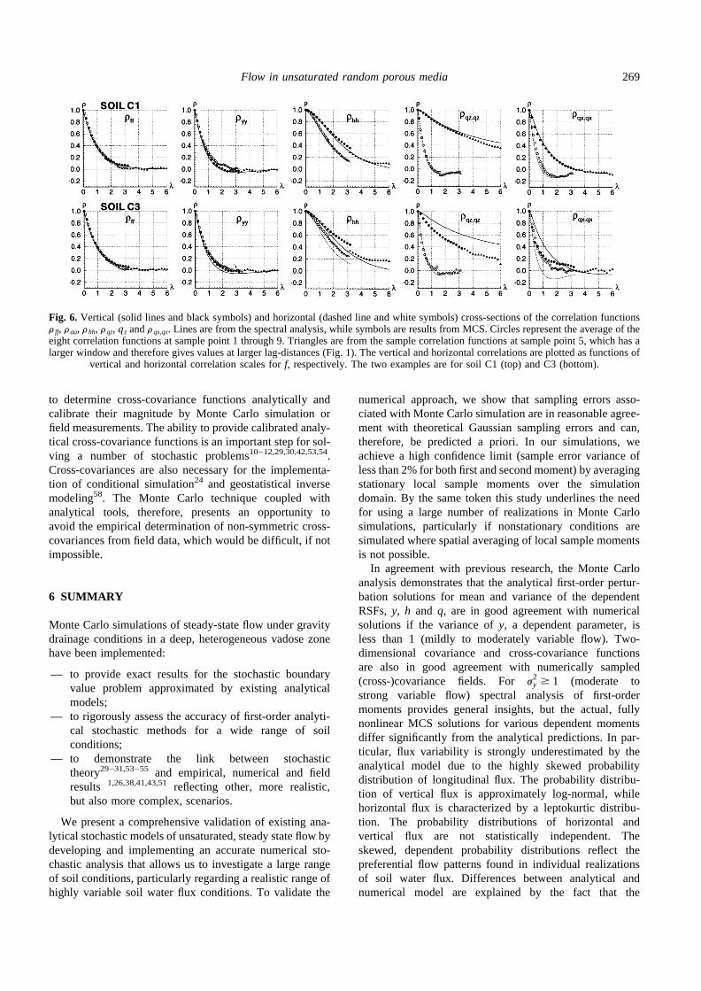
Fig. 5 demonstrates that empirically obtained local (non-averaged) correlation and cross-correlation fields of y and hare in excellent agreement with the theoretical correlationfunctions derived from spectral analysis and reflect thegeneral patterns of unsaturated hydraulic conductivity andsoil water tension distribution found in a hypothetical soilcross-section such as the one discussed above. For refer-ence, the exponential input covariance function off, Cff, isalso shown. The correlation scales ofChh are much largerthan those ofCyy and are anisotropic even if the hydraulicconductivity structure is isotropic, i.e. nonlayered. The headcovariance function reflects the strong spatial continuity,particularly in the horizontal direction, observed in therandom soil of Fig. 2. Overall qualitative agreementbetween analytical and MCS solutions, particularly withrespect to spatial structure, is found at all sites. For betterquantitative comparison, we use vertical and horizontalcross-sections of the (normalized) correlation functionsr ff,ryy, rhh. Examples of correlation functions of both, a mildlyand strongly heterogeneous soil (C1 and C3) are plotted inFig. 6. As expected, analytical and numerical correlationfunctions for f are identical. Similar agreement is foundfor ryy in all soils. Only in strongly heterogeneous soils,the scale of the analytical head correlation function tendsto underestimate the head correlation scale determined fromthe Monte Carlo results. The similarity ofryy or rhh (e.g.Fig. 6) with results by Roth41 indicate that the spectralmethod can be a powerful tool to also approximate stochas-tic analysis of flow in isotropic, Miller-similar media soilwith Van Genuchten parametrization.

Covariancae fields forqx reflect the diagonal patterns,which are observed in individual flux realizations discussedearlier. Covariance ofqx is strongest in the diagonal direc-tions (relative to mean flow direction) and very small invertically overlying or horizontally adjacent location, i.e.in the vertical or horizontal direction. On the other hand,the covariance function ofqz is highly anisotropic with themajor anisotropy axis in mean flow direction. This is notsurprising considering the strong vertical continuity and therelative small lateral extent of the preferential flow channelsdescribed above. Cross-sections of the normalized covar-iance and cross-covariance functions show that analyticalflux correlation functions deviate significantly from numeri-cally determined solutions, ifj2

y . 1. This applies again toboth, wet, texturally very heterogeneous soils (e.g. B3) anddry, texturally rather homogeneous soils (e.g. C3, Fig. 6).Vertical flux correlation functions in the MCS have a shorterlongitudinal correlation scale than analytical correlationfunctions. The transverse hole-type correlation ofqz is accu-rately predicted by spectral first-order analysis, while theanalytical model significantly underestimates the horizontalcorrelation scale ofqx when the flux is highly variable(Fig. 6).

The good agreement between analytically predicted andnumerically derived cross-covariance fields (Fig. 5) isof practical importance for the estimation of cross-covariances. Such agreement allows stochastic modelers

Fig. 5.Comparison of analytical (left) and MCS (right) covarianceand cross-covariance functions for an anisotropic soil (B1). Theshown MCS (cross-)covariances are obtained for sample point 5(see Fig. 1) and based on 1000 sample realization. From top tobottom: covariances of saturated hydraulic conductivity,f, unsa-turated hydraulic conductivity,y, soil water tension,h, verticalflux, qz, and horizontal flux,qx; cross-covariances betweenf andh, betweenf and qz, and betweenf and qx. The x-axes showhorizontal lag-distances, they-axes vertical lag-distances. contourintervals and shading are identical for analytical and MCS results.

All units of length in [cm].


to determine cross-covariance functions analytically andcalibrate their magnitude by Monte Carlo simulation orfield measurements. The ability to provide calibrated analy-tical cross-covariance functions is an important step for sol-ving a number of stochastic problems10–12,29,30,42,53,54.Cross-covariances are also necessary for the implementa-tion of conditional simulation24 and geostatistical inversemodeling58. The Monte Carlo technique coupled withanalytical tools, therefore, presents an opportunity toavoid the empirical determination of non-symmetric cross-covariances from field data, which would be difficult, if notimpossible.

6 SUMMARY

Monte Carlo simulations of steady-state flow under gravitydrainage conditions in a deep, heterogeneous vadose zonehave been implemented:

— to provide exact results for the stochastic boundaryvalue problem approximated by existing analyticalmodels;

— to rigorously assess the accuracy of first-order analyti-cal stochastic methods for a wide range of soilconditions;

— to demonstrate the link between stochastictheory29–31,53–55and empirical, numerical and fieldresults 1,26,38,41,43,51reflecting other, more realistic,but also more complex, scenarios.

We present a comprehensive validation of existing ana-lytical stochastic models of unsaturated, steady state flow bydeveloping and implementing an accurate numerical sto-chastic analysis that allows us to investigate a large rangeof soil conditions, particularly regarding a realistic range ofhighly variable soil water flux conditions. To validate the

numerical approach, we show that sampling errors asso-ciated with Monte Carlo simulation are in reasonable agree-ment with theoretical Gaussian sampling errors and can,therefore, be predicted a priori. In our simulations, weachieve a high confidence limit (sample error variance ofless than 2% for both first and second moment) by averagingstationary local sample moments over the simulationdomain. By the same token this study underlines the needfor using a large number of realizations in Monte Carlosimulations, particularly if nonstationary conditions aresimulated where spatial averaging of local sample momentsis not possible.

In agreement with previous research, the Monte Carloanalysis demonstrates that the analytical first-order pertur-bation solutions for mean and variance of the dependentRSFs,y, h and q, are in good agreement with numericalsolutions if the variance ofy, a dependent parameter, isless than 1 (mildly to moderately variable flow). Two-dimensional covariance and cross-covariance functionsare also in good agreement with numerically sampled(cross-)covariance fields. Forj2

y $ 1 (moderate tostrong variable flow) spectral analysis of first-ordermoments provides general insights, but the actual, fullynonlinear MCS solutions for various dependent momentsdiffer significantly from the analytical predictions. In par-ticular, flux variability is strongly underestimated by theanalytical model due to the highly skewed probabilitydistribution of longitudinal flux. The probability distribu-tion of vertical flux is approximately log-normal, whilehorizontal flux is characterized by a leptokurtic distribu-tion. The probability distributions of horizontal andvertical flux are not statistically independent. Theskewed, dependent probability distributions reflect thepreferential flow patterns found in individual realizationsof soil water flux. Differences between analytical andnumerical model are explained by the fact that the

Fig. 6. Vertical (solid lines and black symbols) and horizontal (dashed line and white symbols) cross-sections of the correlation functionsr ff, raa, rhh, rqz, qz andrqx,qx. Lines are from the spectral analysis, while symbols are results from MCS. Circles represent the average of theeight correlation functions at sample point 1 through 9. Triangles are from the sample correlation functions at sample point 5, which has alarger window and therefore gives values at larger lag-distances (Fig. 1). The vertical and horizontal correlations are plotted as functions of

vertical and horizontal correlation scales forf, respectively. The two examples are for soil C1 (top) and C3 (bottom).


linearized Gaussian analysis does not account for suchhighly nonlinear occurrence of preferential flow.

In agreement with analytical models, numericallydetermined variances forh, y, qx and qz in wet, texturallyheterogeneous soils are found to be similar to those indry, texturally almost homogeneous soils with high varia-bility of unsaturated hydraulic conductivity. The disparitybetween numerical and analytical results for soils withhigh textural variability is shown to be similar to thatfound for relatively homogeneous soils under dry flowconditions. In both cases,j2

y is large. It is, therefore,important to recognize that the application of analyticalstochastic models to relatively homogeneous soils doesnot automatically imply accuracy of first-order approxi-mations. Rather, the analytical spectral model givesaccurate results only if the soil withj2

f , 1 is relativelywet, i.e. soil water flux and not just texture is relativelyhomogeneous.

On a more practical side, where accuracy is oftenmeasured in orders of magnitude rather than in percent,we are encouraged to find that for the large range of soiltexture and soil flux conditions, analytical stochasticmodels are within a factor 2 of the actual moments.For many engineering problems, the application of theanalytical model seems therefore justified, even if flowis highly variable. Other factors, not included in thesimplified conceptual model underlying both the numer-ical and analytical methods presented here, may contri-bute more to estimation errors than the differencesobserved between nonlinear numerical analysis and ana-lytical results. In applications of Monte Carlo simulationsto real world sites, spatially variable soil moisture con-tent, transient flux conditions near the land surface43,nonstationary conditions with spatially variable meanhead (dictated by boundary conditions)26,33, the inclusionof local hysteretic effects33, and the use of realistic para-metrization of the hydraulic conductivity and soil waterretention function41,47 are important features that are notaccounted for by current analytical models. Yet, resultspresented here show encouraging qualitative agreementwith many of those findings indicating that stochasticunsaturated flow theory is capable of capturing manyof the fundamental principles of variably saturated flowdescribed in both field experiments and empirical com-putational experiments despite the underlying simplifyingassymptions.

ACKNOWLEDGEMENTS

This work was funded in part by DOE grant DE-FG02-91-ER61199, the United States Geological Survey, contract#14-08-0001-G2090, and the United States EnvironmentalProtection Agency, contract #R-813899-01-1. We wouldalso like to thank the anonymous reviewers for their manyhelpful comments.

REFERENCES

1. Ababou, R., Three-dimensional flow in random porousmedia. Ph.D. thesis, Department of Civil Engineering,Massachusetts Institute of Technology, Cambridge, MA,1988.

2. Anderson, S. H. and Cassel, D. K. Statistical and autoregres-sive analysis of soil physical properties of Portsmouth sandyloam. Soil Sci. Soc. Am. J., 1986,49, 1096–1104.

3. Bakr, A. A., Gelhar, L. W., Gutjahr, A. L. and McMillan, J.R. Stochastic analysis of the effect of spatial variability insubsurface flows, 1: comparison of one- and three-dimensional flows.Water Resour. Res., 1978,14, 263–271.

4. Bellin, A., Salandin, P. and Rinaldo, A. Simulation of dis-persion in heterogeneous porous formations: statistics, first-order theories, convergence of computations.Water Resour.Res., 1992,28, 2211–2227.

5. Brigham, E. O.,The Fast Fourier Transform and its Applica-tions. Englewood Cliffs, N.J., 1988.

6. Ciollaro, G. and Comegna, V. Spatial variability of soilhydraulic properties of a psammetic palexeralf soil ofSouth Italy. Acta Horticulturae, Int. Soc. for HorticulturalScience, 1988,228,61–71.

7. Crosby, J. W., Johnstone, D. L., Drake, C. H. and Renston,R. L. Migration of pollutants in a glacial outwash environ-ment, 1.Water Resour. Res., 1968,4, 1095–1113.



10. Cvetkovic, V., Shapiro, A. M. and Dagan, G. A solute fluxapproach to transport in heterogeneous formations, 2. Uncer-tainty analysis.Water Resour. Res., 1992,28, 1377–1388.

11. Dagan, G. Solute transport in heterogeneous porous forma-tions. J. Fluid Mechanics, 1984,145,151–177.

12. Dagan, G. Theory of solute transport by groundwater.Ann.Rev. Fluid Mech., 1987,19, 183–215.

13. Dagan, G.,Flow and Transport in Porous Formations.Springer, Berlin, 1989, 485 pp.

14. Gardner, W. R. Some steady state solutions of unsaturatedmoisture flow equations with applications to evaporate froma water table.Soil Sci., 1958,85, 228–232.

15. Gelhar, L. W.,Stochastic Subsurface Hydrology. Prentice-Hall, Englewood Cliffs, N.J., 1993, 390 pp.

16. Glass, R. J., Steenhuis, T. S. and Parlange, J.-Y. Wettingfront instability as a rapid and far-reaching hydrologicalprocess in the vadose zone.J. of Contam. Hydrol., 1988,3,207–226.

17. Grennholtz, D. E., Yeh, T.-C. J., Nash, M. S. B. andWierenga, P. J. Geostatistical analysis of soil hydrologicalproperties in a field plot.J. of Contam. Hydrol., 1988, 3,227–250.

18. Greminger, P. J., Sud, Y. K. and Nielsen, D. R. Spatial varia-bility of field-measured soil–water characteristics.Soil Sci.Soc. Am. J., 1985,49, 1075–1082.

19. Gutjahr, A. L., Fast Fourier transforms for random fieldeneration. Project Report for Los Alamos Grant to NewMexico Tech, Contract number 4-R58-2690R, Departmentof Mathematics, New Mexico Tech, Socorro, New Mexico,1989.

20. Haan, C. T.,Statistical Methods in Hydrology. Iowa StateUniversity Press, Ames, Iowa, 1977, 378 pp.

21. Harter, T. and Yeh, T. C. J. An efficient method for simu-lating steady unsaturated flow in random porous media: usingan analytical perturbation solution as initial guess to a


numerical model.Water Resour. Res., 1993, 29, 4139–4149.

22. Harter, T., Unconditional and conditional simulation offlow and transport in heterogeneous, variably saturatedporous media. Ph.D. dissertation, University of Arizona,1994.

23. Harter, T. and Yeh, T.-C. J. Stochastic analysis of solutetransport in heterogeneous, variably saturated porousmedia.Water Resour. Res., 1996,32, 1585–1595.

24. Harter, T. and Yeh, T.-C. J. Conditional stochastic analysis ofsolute transport in heterogeneous, variably saturated soils.Water Resour. Res., 1996,32, 1597–1609.

25. Hillel, D., Fundamentals of Soil Physics. Academic Press,New York, 1980, 413 pp.

26. Hopmans, J. W., Schukking, H. and Torfs, P. J. J. F. Two-dimensional steady state unsaturated water flow in hetero-geneous soils with autocorrelated soil hydraulic properties.Water Resour. Res., 1988,24, 2005–2017.

27. Kalos, M. H. and Whitlock, P.A.,Monte Carlo Methods,vol. 1. Wiley, New York, 1986, 186 pp.

28. Lauren, J. G., Wagenet, R. J., Bouma, J. and Wonston, J. H.M. Variability of saturated hydraulic conductivity in a glos-saquic hapludalf with macropores.Soil Sci., 1988, 145,2005–2017.

29. Mantaglou, A. and Gelhar, L. W. Stochastic modeling oflarge-scale transient unsaturated flow systems.WaterResour. Res., 1987,23, 37–46.

30. Mantoglou, A. and Gelhar, L. W. Capillary tension headvariance, mean soil moisture content, and effective specificsoil moisture capacity of transient unsaturated flow in strati-fied soils.Water Resour. Res., 1987,23, 47–56.

31. Mantoglou, A. and Gelhar, L. W. Effective hydraulic con-ductivities of transient unsaturated flow in stratified soils.Water Resour. Res., 1987,23, 57–67.

32. Mizell, S. A., Gutjahr, A. L. and Gelhar, L. W. Stochasticanalysis of spatial variability in two-dimensional steadygroundwater flow assuming stationary and nonstationaryheads.Water Resour. Res., 1982,18, 1053–1067.

33. McCord, J. T., Stephens, D. B. and Wilson, J.L. Hysteresisand state-dependent anisotropy in modeling unsaturated hill-slope hydrologic processes.Water Resour. Res., 1991, 27,1501–1518.

34. Moreno, L., Tsang, Y. W., Tsang, C. F., Hale, F. V. andNeretnieks, I. Flow and tracer transport in a single fracture:a stochastic model and its relation to some field observations.Water Resour. Res., 1989,24, 2033–2048.

35. Moreno, L. and Tsang, C. F. Flow channeling in stronglyheterogeneous porous media: A numerical study.WaterResour. Res., 1994,30, 1421–1430.

36. Neuman, S. P., Stochastic approach to subsurface flow andtransport: a view to the future. In: Proceedings, Workshop onStochastic Subsurface Hydrology, Paris, January 1995.

37. Nielsen, D. R., Biggar, J. W. and Erh, K. T. Spatial varia-bility of field measured soil–water properties.Hilgardia,1973,42, 215–260.

38. Polmann, D. J., McLaughlin, D., Luis, S., Gelhar, L. W. andAbabou, R. Stochastic modeling of large-scale flow inheterogeneous unsaturated soils.Water Resour. Res., 1991,27, 1447–1458.

39. Press, W. H., Vetterling, W. T., Teukolsky, S.A. andFlannery, B.P.,Numerical Recipes in FORTRAN, 2nd edn.Cambridge University Press, Cambridge, 1992.

40. Priestley, M. B.,Spectral Analysis and Time Series. Aca-demic Press, San Diego, pp. 890, 1981.

41. Roth, K. Steady state flow in an unsaturated, two-dimensional, macroscopically homogeneous Miller-similarmedium.Water Resour. Res., 1995,31, 2127–2140.

42. Rubin, Y. Stochastic modeling of macrodispersion in

heterogeneous porous media.Water Resour. Res., 1990,26,114–133.

43. Russo, D. Stochastic analysis of simulated vadose zonesolute transport in a vertical cross section of heterogeneoussoils during nonsteady water flow.Water Resour. Res., 1991,27, 267–284.

44. Russo, D. Stochastic modeling of macrodispersion for solutetransport in a heterogeneous unsaturated porous formation.Water Resour. Res., 1993,29, 383–397.

45. Russo, D. Stochastic modeling of solute flux in a hetero-geneous partially saturated porous formation.WaterResour. Res., 1993,29, 1731–1744.

46. Unlu, K., Nielsen, D. R. and Biggar, J. W. Stochastic analysisof unsaturated flow: one-dimensional Monte Carlo simula-tions and comparisons with spectral perturbation analysisand field observations.Water Resour. Res., 1990, 26,2207–2218.

47. Van Genuchten, M. Th. A closed-form equation for predict-ing the hydraulic conductivity of unsaturated soils.Soil Sci.Soc. Am. J., 1980,44, 892–898.

48. Vieira, S. R., Nielsen, D. R. and Biggar, J. W. Spatial varia-bility of field measured infiltration rate.Soil Sci. Soc. Am. J.,1981,45, 1040–1048.

49. White, I. and Sully, M. J. On the variability and use of thehydraulic conductivitya parameter in stochastic treatmentsof unsaturated flow.Water Resour. Res., 1992,28, 209–213.

50. Wierenga, P. J., Toorman, A. F., Hudson, D.B., Vinson, J.,Nash, M. and Hills, R.G., Soil physical properties at the LasCruces trench site, UREG/CR-5441, 1989.

51. Wierenga, P. J., Hills, R. G. and Hudson, D. B. The LasCruces trench site: characterization, experimental results,and one-dimensional flow.Water Resour. Res., 1991, 27,2695–2706.

52. Wilson, L. G. and De Cook, K. J. Field observations onchanges in the subsurface water regime during influentseepage in the Santa Cruz River.Water Resour. Res., 1968,4, 1219–1234.

53. Yeh, T.-C. J., Gelhar, L. W. and Gutjahr, A. L. Stochasticanalysis of unsaturated flow in heterogeneous soils, 1: statis-tically isotropic media.Water Resour. Res., 1985,21,447–456.

54. Yeh, T.-C. J., Gelhar, L. W. and Gutjahr, A. L. Stochasticanalysis of unsaturated flow in heterogeneous soils, 2: statis-tically anisotropic media with variable,a. Water Resour.Res., 1985,21, 457–464.

55. Yeh, T.-C. J., Gelhar, L. W. and Gutjahr, A. L. Stochasticanalysis of unsaturated flow in heterogeneous soils, 3: observa-tions and applications.Water Resour. Res., 1985,21,465–471.

56. Yeh, T.-C. J. One-dimensional steady state infiltration inheterogeneous soils.Water Resour. Res., 1989, 25, 2149–2158.

57. Yeh, T.-C. J., Srivastava, R., Guzman, A. and Harter, T. Anumerical model for two-dimensional water flow andchemical transport.Ground Water, 1993,32, 2–11.

58. Yeh, T.-C. J. and Zhang, J. A geostatistical invese method forvariably saturated flow in the vadose zone.Water Resour.Res., 1996,32, 2757–2766.

59. Yevjevich, V. M.,Stochastic Processes in Hydrology. WaterResources Publications, Fort Collins, CO, 1972.

60. Zaslavsky, D. and Sinai, G. Surface hydrology, IV. Flow insloping layered soil.J. Hydraul. Div. Am. Soc. Civ. Engng,1981,107(HY1), 53–64.

APPENDIX A

A derivation of the spectral moments is given in Yeh etal.53,54assuming thata is normally distributed. The analysis


here, however, assumes thata is lognormally distributed.Writing exp (A þ a9) ¼ exp (A) exp (a9), expanding theexponential perturbation term in a Taylor series, truncatingthe Taylor series to first-order, and neglecting second- andhigher-order terms, the first-order perturbation approxima-tion of the unsaturated hydraulic conductivity is

Yþ y9 ¼ (F þ HG) þ (f 9 þ Gh9 þ HGa9), (A1)

whereG ; exp (A). Following the analysis of Yeh et al.53,54

for gravity flow, the spectral solution forh9, dZh9, thenbecomes

dZh9 ¼ikz(dZf 9 þ HGdZa9)

(k2x þ k2

z ¹ iGkz)(A2)

where dZf and dZa9 are the spectral representations off 9anda940. The spectral and cross-spectral density functionsSpq(k), for pressure head, hydraulic conductivity and fluxperturbations in the special case of identical correlationfunctions inf anda are:

Shh ¼k2

z

(k2x þ k2

z)2 þG2k2z[1þ 2rzHG þ (zHG)2]Sff (A3)

Sfh ¼ [ ¹Gk2z þ ikz(k2

x þ k2z)]

(Sff þ HGSfa)(k2

x þ k2z)2 þ (G2k2

z)(A4)

Sah ¼zr þ z2HG

1þ zrHGSfh (A5)

Syy ¼ 1þ¹ k2

zG2

(k2x þ k2

z)2 þ G2k2z

� �[1þ 2rzHG þ (zHG)2]Sff

(A6)

Sqx:qx ¼ K2m

k2xk2

z

(k2x þ k2

z)2 þ G2k2z[1þ 2rzHG þ (zHG)2]Sff

(A7)

Sqz:qz¼ K2m 1¹

k2z(G2 þ k2

z) þ 2k2xk2

z

(k2x þ k2

z)2 þ G2k2z

� �3 [1þ 2rzHG þ (zHG)2]Sff :

Sff and Saa may be obtained analytically or by numericalintegration from the assumed covariance functions3,32.The cross-spectral densitySfa depends on the desiredcross-correlation betweenf(x) and a9(x þ y). IfCaa=j

2a ¼ Cff =j

2f , i.e. the correlation functions ofa9 and f 9

are identical, then

Saa ¼ z2Sff (A8)

Saf ¼ zrSff :

In this study, all spectrally derived covariances and cross-covariances except those forf anda, are evaluated numeri-cally through an inverse fast Fourier transform (inverseFFT5,39 of the spectral density functions in Appendix A.For the inverse FFT,Spq(k) is discretized such that the two-dimensional covarianceCf (y) of f has 10 grid-points perl f. It is evaluated at ally # 100l f.


flow in unsatruated random porus media, nonlinear...

Documents