Contents lists available at ScienceDirect

Flow Measurement and Instrumentation

journal homepage: www.elsevier.com/locate/flowmeasinst

On the estimation of free-surface turbulence using ultrasonic sensors

G. Zhanga, D. Valerob,⁎,1, D.B. Bungb,2, H. Chansona,3

a Dept. of Hydraulic Engineering, School of Civil Engineering, The University of Queensland, Brisbane, QLD 4072, AustraliabHydraulic Engineering Section, FH Aachen University of Applied Sciences, Bayernallee 9, Aachen 52066, Germany

A R T I C L E I N F O

Keywords:Acoustic displacement meterFree-surface dynamicsWavePower spectraAir-water flowsStepped spillway

A B S T R A C T

Accurate determination of free-surface dynamics has attracted much research attention during the past decadeand has important applications in many environmental and water related areas. In this study, the free-surfacedynamics in several turbulent flows commonly found in nature were investigated using a synchronised setupconsisting of an ultrasonic sensor and a high-speed video camera. Basic sensor capabilities were examined in dryconditions to allow for a better characterisation of the present sensor model. The ultrasonic sensor was found toadequately reproduce free-surface dynamics up to the second order, especially in two-dimensional scenarioswith the most energetic modes in the low frequency range. The sensor frequency response was satisfactory in thesub-20 Hz band, and its signal quality may be further improved by low-pass filtering prior to digitisation. Theapplication of the USS to characterise entrapped air in high-velocity flows is also discussed.

1. Introduction

Most common environmental flows are turbulent free-surface flows,transporting all sorts of waves ranging from the small-scale capillarywaves to the breaking waves of the sea, which can be several metres inscale. While the free surface of a liquid in equilibrium is plane, underthe action of a perturbation it will move from equilibrium, propagatingthis motion through the domain due to gravity and surface tension [36].Despite major efforts (among others: [21,13,42,58]), understanding offree-surface turbulence is not available, becoming a bottleneck in manyenvironmental applications. Although true relation between waterturbulence properties and free-surface oscillations is not yet disclosed,such a relationship seems to exist [13,22,58,68–70]. A study of theturbulence properties of the free-surface may help understanding theprocesses happening beneath, shedding light on mass, momentum andheat transfer across gas-liquid interfaces. Additionally, the existence ofa free-surface modifies the flow characteristics beneath, which alsointeract non-linearly with the free-surface [28,63,68]. Near the free-surface, turbulence anisotropy, altogether with shear reduction, seemsto be a common feature in most studies [18,22,24]. Roussinova et al.[56], following the previous study of Nezu [46], suggested that the free-surface behaves as a “weak wall” where normal velocity fluctuationsare countered by surface tension. Gualtieri and Gualtieri [20]

conceptualized the free-surface interaction with turbulence to predictgas-transfer rates. Murzyn and Chanson [43] suggested that free-surfaceoscillations are linked to the turbulent kinetic energy per unit volume.Roussinova et al. [56] also observed that presence of a free-surface canyield secondary flows within the water body, which is in agreementwith the hypothesis resulting of the study of Tamburrino and Gulliver[62]. Guo and Shen [22] illustrated the surface blockage effect and thevanishing of the shear stress and, later, Guo and Shen [23] studied thecomplex effect of waves on turbulence underneath. Recently, Nicholset al. [48] proposed a simple model for free-surface dynamics that mayhelp in future to link the surface kinematics to the underlying complexturbulence phenomenon. Zhong et al. [77] found evidence of super-streamwise vortices, previously observed by Gulliver and Halverson[21], existing universally as free-surface coherent structures occurringin open channel flows.

Many processes can originate free-surface perturbations. Some stu-dies have been conducted in the past, relating the external air floweffect to the generation of waves in the sea [27,29,39,74]. Yet free-surface can be also perturbed by other causes. Schvidchenko andPender [60] found that the bursting phenomenon, contributing to se-diment transport, generates eddies reaching the free-surface. This is inagreement with the previous study of Schvidchenko and Pender [59]who noticed that relative flow depth affects the erosion process; which

https://doi.org/10.1016/j.flowmeasinst.2018.02.009Received 15 November 2016; Received in revised form 5 February 2018; Accepted 11 February 2018

⁎ Correspondence to: Research Group of Hydraulics in Environmental and Civil Engineering (HECE), University of Liège, Chemin des Chevreuils, 1, building B52/3 floor +1, 4000Liège, Belgium.

1 ORCID: 0000-0002-7127-7547.2 ORCID: 0000-0001-8057-1193.3 ORCID: 0000-0002-2016-9650.

E-mail address: valero@fh-aachen.de (D. Valero).

Flow Measurement and Instrumentation 60 (2018) 171–184

Available online 13 February 20180955-5986/ © 2018 Elsevier Ltd. All rights reserved.

T

was later observed and further explained by the numerical study ofChang and Constantinescu [6]. Similarly, Dabiri [13] showed that thefree-surface deformation may be strongly correlated to the normalsurface vorticity produced in a vertical shear layer, showing also howsimultaneously the presence of a free-surface alters its structure. Thus,not only turbulence may affect the free-surface but also the free-surfacecan affect the turbulence. Similarly, Roy et al. [57] observed thatprocesses taking place on a gravel bed could reach the free-surface(megabursts). Savelsberg [58] found that free-surface roughness islinked to the sub-surface turbulence. Guo and Shen [22] numericallystudied the free-surface roughness resulting from the isotropic turbu-lence generated underneath the free-surface, concluding that motion ofthe free-surface is composed of propagating waves and turbulencegenerated roughness. Horoshenkov et al. [25] noticed evidence ofwaves produced by turbulence generated over rough sediment surfaces,which showed considerably different phase velocity – frequency rela-tion than common gravity waves. Johnson and Cowen [30] were able toestimate flow discharges based on free-surface turbulent properties.

Waves have been also observed in the non-aerated region ofspillway flows [1,15,66–68,75]. Valero and Bung [66] observed thedynamics of these waves in the inception point location and Valero andBung [67] described the different types of waves, pointing out the roleof air-water friction in the wave generation when high velocity flowstake place. Another clear evidence of free-surface turbulence - due tothe underlying hydrodynamic processes - can be observed in hydraulicjumps [10], which have been also investigated previously using ultra-sonic sensors [5,69]. Hydraulic jump quasi-periodic features were firstpointed out by Nebbia [45], in a phenomenon amplified by the chan-ging jump due to erosion. Since then, dynamic processes resulting fromthe high velocity flow impacting the slower velocity downstream flowhave attracted researchers’ interest. Long et al. [38] used imagingtechniques; Mossa [40] and Mossa et al. [41] used a pressure trans-ducer, a resistance probe and a video camera to study periodic andquasi-periodic phenomenon inside the jump. During the last decade,free-surface fluctuations of hydraulic jump rollers were studied mainlyby means of ultrasonic sensors, yielding a greater insight on the overallflow turbulence. Koch and Chanson [34] first used ultrasonic sensors tostudy undular and breaking bores. Additional studies using ultrasonicsensors [35,43,5,71,72] provided deeper insight on free-surface tur-bulence in stationary hydraulic jumps. Additionally, this technique hasbeen also applied to high velocity spillway flows [3,4]. Its capability tostudy both aerated and non-aerated regions has been shown [66] ob-taining characteristic flow depths, its oscillations and waves frequenciesin stepped spillway flows [4]; however, larger deviation can be ex-pected in the study of the aerated region [15]. Other studies have re-lated ultrasonic measurement to characteristic aeration levels: h50 – h60for a slightly aerated bubbly column [9], h60 – h80 for the hydraulicjump roller flow [35] and h75 for aerated spillway flows [4]; with hX themean water depth associated with a mean air concentration =C X (%).Murzyn and Chanson [43] and Chachereau and Chanson [5], suggestedotherwise that the ultrasonic measurement in a hydraulic jump mightcorrespond to a thin region below the upper free-surface region butalways over the air-water shear layer.

Albeit different measurement techniques are available, ultrasonicsensors may be of special interest in many applications because of theirrobustness and non-intrusive nature. Traditional point gauge allowsstatic measurements usually at an accuracy of 0.1 mm. Wave gauges canadditionally perform dynamic measurements, similarly to ultrasonicsensors, but are subject to temperature changes within the water bodyand also flow perturbation or sensors interference can happen.Naturally, sensors interference can also happen between ultrasonicsensors and temperature effect must be contemplated, but non-intru-siveness can represent an advantage. Main benefits of other techniquescan be met by ultrasonic sensors, but its performance has to be carefullyassessed to ensure reliable non-intrusive measurements of free-surfaceprofiles, free-surface fluctuations, free-surface correlation time scales,

free-surface wave celerity and frequencies [15,4,43,5,67]. Additionally,how the footprint relates to the measurement has not been still as-sessed.

The promising future of other acoustic techniques for velocity[37,44,55,64] and free-surface determination [26,33,47] motivates thisresearch which aims to assess the performance of a pulse-echo ultra-sonic sensor for common environmental flows. Different common en-vironmental flows have been studied both by means of ultrasonic sen-sors and a high-speed camera in the following sections. The manuscriptis structured as follows: performance of the ultrasonic sensor has firstbeen studied in dry conditions in Section 3. In Section 4.2, a 2D waveflume investigation is presented. Section 4.3 presents study of the ul-trasonic sensor accuracy in the non-aerated region of a spillway; whichrepresents a 3D wavy open channel flow, more challenging than thecounterpart subcritical flows commonly studied. Section 4.4 presentssome comments on the ultrasonic sensors’ performance and capabilitiesfor aerated flows which is further completed by the analysis presentedin Section 4.5 for the air content estimation. Finally, Section 5 collectsthe main conclusions of the presented study.

2. Experimental setup and instrumentation

2.1. Instrumentation

The primary instrumentation used in the present investigation in-cluded three cylindrical microsonic™ mic+130 ultrasonic sensors (USS)for analogue free-surface measurements plugged to a computer througha HBM™ QuantumX 840A amplifier. The sensors utilise a pulse-echoprinciple and operate at a transducer frequency of 200 kHz (note thatthis frequency is related to resolution but not to sampling rate). Theacoustic sensing range is 0.2–2.0m with corresponding resolutions be-tween 0.18mm and 0.57mm (specified by the sensors’ manufacturer),and a “blind zone” is defined for 0–0.2m. The size of the detection zonewas between 0.05m and 0.15m, yielding a minimum expected precisionof 1.1% (for wavelengths greater than the detection zone size). Errorsdue to temperature drift are internally compensated. The sensors are IP67 rated and were well suited for the laboratory operating conditions.Note that only one sensor model was tested herein.

For comparison, data were recorded by a Phantom™ M120 high-speed video camera synchronised with the USS sensors via an in-housePython script. The camera was capable of recording at up to 730 fps at aresolution of 1920 by 1200 pixels (throughput: 1.6 Gpx/s), and it waspossible to increase the frame rate by reducing the image resolution.Two 500W halogen lights were customarily placed to achieve visuallyhomogenous illumination across the scene. The free-surface profileswere deduced from the digital image sequences using various imageprocessing techniques depending on the flow type of each experiment.The camera was sampled at 100 fps at a resolution of 1920 by 1200pixels for all experiments. The sample rate was selected as a compro-mise between precision and storage requirements.

Synchronisation of sensors was achieved by simultaneously trig-gering the USS and camera sample clocks. When the USS clock fires, aPython script sends a trigger to the camera clock by calling theWindows application programming interfaces (Win32 API). Any mis-alignment due to software delay (typically less than 0.1 s) was com-pensated using a cross-correlation technique, corrected to the nearestsample (i.e. 0.02 s). The data acquisition software were Catman v3.3(HBM™) and DaVis v8.1 (LaVision™) for the USS and camera respec-tively. The USS and camera were respectively sampled at 50 Hz and100 Hz for 30 s during all experiments. The higher camera samplingrate helps to facilitate better matching between the signals. The sam-pling parameters were chosen herein to achieve a balance betweenaccurate signal reconstruction and hardware capacity (especially thecamera). It is acknowledged that a minimum of 5000–10,000 sampleswould be desirable to characterise turbulence properties up to thesecond order (i.e. variance) (e.g. [31,11]).

G. Zhang et al. Flow Measurement and Instrumentation 60 (2018) 171–184

172

Detailed void fraction measurements were performed with a dual-tip optical fibre probe (A2 Photonic Sensors™). The data were derivedfrom the leading tip signal, sampled for 45 s at 1MHz, which wasconsiderably above the minimum recommended sample rate for similartechniques [16].

2.2. Experimental facilities

Present investigations were undertaken in relatively large-sizephysical models in the FH Aachen Hydraulics Laboratory (Aachen,Germany). The model discharge was delivered through a closed conduitand was regulated by a frequency regulator (Grundfos™ blueflux). Anelectromagnetic flow meter (Krohne™ WATERFLUX 3100 W) was usedto measure the discharge, with an expected error of 0.3%.

The first experiment, for validation purposes, was performed in awave flume of dimensions 0.58m wide by 0.80m high and 12m long. Asketch of the facility is shown in Fig. 1. The discharge was suppliedfrom an upstream intake and drained through the gaps between severalrows of flap gates located at the downstream end of the flume. A dis-charge of 0.015–0.020m3/s was maintained in the flume such that thewater depth was visually constant, prior to any waves being generated.The first train of waves was generated by manually operating a flat

plate at the downstream end of the flume at approximately 0.5 Hz. Thewaves propagated upstream and were reflected by a sluice gate locatednear the upstream end of the channel. The stimulus was applied con-tinuously to produce a range of complex and uncontrolled waves withcharacteristic heights between 0.005m and 0.20m, observed synchro-nously by both the camera and USS. An average water depth of ap-proximately 0.40m was maintained during this process.

The high-speed video camera was set up beside the channel with afield of view measuring 0.138m by 0.86m (landscape). The halogenlights were placed such that the water surface was naturally enhancedwhen observed from the camera, and a dark background was set toimprove contrast. The first USS sensor was mounted approximately0.10m inside the sidewall and 0.40m above the water surface, with ameasuring zone of approximately 0.10m in diameter. A second USSsensor was mounted in symmetry with the primary sensor about thechannel centreline for checking the two-dimensionality of the waves. Itwas found that mismatches between the USS and high-speed cameradata were minimised when waves were approximately two-dimen-sional. However, small discrepancies may arise due to surface tensionand wall effects.

Further tests were performed in a 1V:2H (26.6°) stepped spillwaymodel to study the feasibility of USS in scenarios with increased free-

Fig. 1. Sketch of the setup in the 2D wave experiment.

Fig. 2. Stepped spillway experimental configuration in the non-aerated and aerated measurements.

G. Zhang et al. Flow Measurement and Instrumentation 60 (2018) 171–184

173

surface geometric complexity in high velocity supercritical flows. Asketch of the facility is shown in Fig. 2. The model was 0.50m wide andhad a total drop height of 1.74m, lined with 0.06m×0.12m (rise× run) flat impervious steps (θ =26.6°). The chute inflow was con-trolled by a 1.0m long broad-crested weir with discharge delivered bythe same system as for the wave flume. Free-surface fluctuations weresampled with a rail-mounted USS at approximately 0.07m inside thesidewall. The high-speed video camera was mounted beside the channelwith a field-of-view of about two step cavities wide. The experimentalflow conditions are summarised in Table 1, with Reynolds numbers(Re) ranging from 9x104 to 1.1x105.

3. Sensor calibration and signal characterisation

3.1. Presentation

The USSs were first tested in dry conditions to observe their cap-abilities and signal characteristics. The voltage responses of each USSwas examined by placing a perpendicular solid plastic surface at dif-ferent distances from the sensor. The voltage–distance relationship waslinear throughout the measuring range of the sensor. A “blind zone” anda “far field” were respectively identified close to and away from thesensor as per Fig. 3. The standard deviation of each static measurementwas interpreted as the measurement uncertainty, which remained ap-proximately constant over the full detectable range. The results showedno preferential measuring distance despite the maximum detected de-viation (around 1mm) seemed to increase with distance (Fig. 3). In-formation on Fig. 3 was sampled over 30 s.

The footprint of the USS is shown in Fig. 4. This footprint wasmeasured by fixing the sensor and repeatedly introducing a plate atdifferent distances away from the transducer and recording the distancefrom the centreline at which the USS detected the obstacle. The USSsignal changes in a space of around 1mm. The sensing cone shown inFig. 4 spreads with distance at an angle of 4°. The sensor allows internaladjustments of the detection zone (options: “normal/slight”), althoughno significant difference was found between the options (Fig. 4). Dif-ficulty in detecting steeper waves by similar sensors was noted in sev-eral previous studies [15,34,4]. The sensitivity of the sensing error to

surface slope (α) variations is examined in Fig. 4 (right). It was observedthat outliers did not occur for surface slopes flatter than 13.5°.

The temperature dependence of the USSs was investigated by un-dertaking long measurements of 12 h at a sample rate of 1 Hz. In Fig. 5,only the data for the first 6 h are shown for clarity. Notably, most sig-nificant changes in the sample mean were observed during the firsthour. Consequently, a minimum warm-up period of 1 h as advised bythe manufacturer after which calibration shall be required prior to dataacquisition.

3.2. Sample rate, aliasing and noise

The USS operates by measuring the time lag between the emittedand reflected ultrasound pulses. The pulses are emitted at a pre-estab-lished interval to ensure that all meaningful echoes are captured beforea new pulse is broadcast. The shortest pulse interval determines themaximum frequency that needs to be resolved by the data acquisition(DAQ) system of which the sampling frequency must be appropriatelychosen. The Nyquist sampling theorem [49,50,61] requires this to beequal to or greater than twice the maximum frequency present in thesignal (i.e. Nyquist frequency). This minimum sampling frequency isknown as the Nyquist rate. Failure to satisfy the Nyquist criterion willresult in a higher frequency signal with frequency f manifesting as alower frequency component with an apparent frequency equalling |fs -f| where fs is the sampling frequency. As such, the original signal can nolonger be reconstructed by low pass filtering without distortion and thisis referred to as aliasing [50].

The effects of sampling rate and analogue filtering were first in-vestigated by examining the USS signal power spectral densities plottedin Fig. 6. The data were sampled with the USS facing a fixed flat surfaceperpendicular to the sensor centreline. The signal mean was removedprior to computing the power spectral density functions. The over-sampled power spectral density function at 1200 Hz (Fig. 6 black/greylines) shows a steep roll-off above 20 Hz and an isolated peak at 60 Hz.The latter peak likely arose from the connected electronics, as the localmain frequency was 50 Hz. The USS signal was therefore approximatelybandlimited up to 20 Hz (i.e. cut-off), and that a minimum samplingrate of 50 Hz is recommended to minimise aliasing distortion. Note thata minimum sampling rate of 10 times the Nyquist frequency (i.e. 250 Hzfor a sampling rate of 50 Hz) may be required for accurate waveformreproduction [2].

The use of analogue low-pass filtering prior to digitisation helpsprevent aliasing distortion. Fig. 6 (black dash) shows a USS signal di-gitised at 50 Hz post low-pass filtering (Butterworth with a cut-off fre-quency of 20 Hz). Comparison with the oversampled power spectraldensity function at 1200 Hz (Fig. 6 black line) reveals a good re-production of the spectral components up to the Nyquist frequency. Thebuilt-in analogue Butterworth filter was effective at removing aliases

Table 1Experimental flow conditions for the 3D free-surface roughness experiment in the steppedspillway model.

Location q (m2/s) Width (m) Slope, θ (°) Re Remarks

Step 4 0.090 0.5 26.6 9.0×104 Clear water skimmingflow0.110 1.1×105

Step 20 0.090 0.5 26.6 9.0×104 Aerated skimmingflow0.110 1.1×105

Fig. 3. Linear calibration curve (left), standard deviation (std) and maximum value (max) of a static measurement at different distances from the USS (right) without any signal filtering.

G. Zhang et al. Flow Measurement and Instrumentation 60 (2018) 171–184

174

from frequencies above the Nyquist frequency (25 Hz) without sig-nificantly degrading the passband (0 – 20 Hz). Note that low-pass fil-tering may not always be required on account of the much lower USSfrequency response above 20 Hz. The filter implementations also differamongst analogue to digital conversion (ADC) systems. For simplicity,all analogue filters are disabled herein.

A review of Fig. 6 indicates that a minimum sampling rate of 50 Hzmay be required. The typical USS noise power spectral density functionsampled at this rate, with all filters disabled, is shown in Fig. 7. Thedata revealed an aliased peak at 10 Hz due to power fluctuations, which

may not be important if the signal-to-noise ratio is large. The powerspectral density function was approximately white (i.e. equal intensityin all frequencies) up to the Nyquist frequency (25 Hz) due to thecombined effects of temperature, surface-characteristics and intrinsicelectrical noise of the system.

3.3. Detectable frequencies and uncertainty involved in the wave amplitudedetermination

Any USS sensor has a limited response time which represents alimitation when measuring high frequencies. In order to investigate theperformance of the USS at those frequencies, experiments with a

Fig. 4. (Left) Footprint of a USS measured at the laboratory (present model). Objects are detected when placed within the sensor’s detection radius, which is a function of the surfaceroughness. (Right) Standard deviation dependence on the surface slope.

Fig. 5. Long time record of USS signals for two different sensors. Temperature has sig-nificant effects on sensor data during the first hour. The initially measured distance (y0) issubtracted to the recording.

Fig. 6. Effects of sampling rate and analogue filtering on USS signal power spectral density function (PSD). BW for Butterworth filtered signals.

Fig. 7. Typical noise power spectral density function (PSD) of a USS signal. Samplingrate: 50 Hz. Sampling Duration: 30 s.

G. Zhang et al. Flow Measurement and Instrumentation 60 (2018) 171–184

175

vibrating plate were conducted.A PVC plate was fixed over an aluminium bar (isel™, uni-

versalprofile PU50), whose combination of elasticity modulus (E=70GPa), density (1.22 kg/m), inertias (in both transversal axis, Ix=10.99 cm4 and Iy =2.81 cm4) and length (up to 3m) allowed studyof frequencies below 30 Hz. The bar was fixed to a solid and massivemetal structure so that a cantilever was resulted with the plastic plateclose to the bar extremity. Two USS sensors were placed at 0.50mabove the plastic plate and were separated by 0.20m to avoid inter-ference. The bar was shortened iteratively, thereby increasing thestiffness of the system. For each length investigated, the bar was sti-mulated with a single impact producing oscillations with amplitudessignificantly above those of the USS noise. Two bars were used, prof-iting from both transversal inertias to cover a wider range of fre-quencies. The high-speed camera was employed using significantlyhigher sample rates (over ten times the bar frequency) to obtain the realfrequency of the vibrating system. The frequencies in both cases wereestimated by counting zero-crossings over the first second after theimpact.

A close correspondence is observed between the camera and USSfrequencies up to 20 Hz, while frequencies above 20 Hz were increas-ingly underreported by the USS. To gain further insight, a simple casewhere a plate oscillates as described by the sine equation is considered:

′ = +h t A π f t φ( ) sin(2 ) (1)

where A is the amplitude, f the frequency of the oscillation, t the timeand φ the initial phase shift. If the speed of the plate is considerablysmaller than the speed of the sound ( ≪v c), then it is reasonable toassume that the sensor will see the object at every sampling time asstatic, i.e.: as a fixed plate at a different height each time.

For different values of f , Eq. (1) can be used to generate a newsignal. A hundred different frequencies with a hundred different initialphase shifts (randomly initialised) have been used to render syntheticsignals with N =100 no. of complete periods. Zero-crossings can becounted in a similar manner to that for the vibrating plate tests, thusrecovering the same original frequency. This signal can also be re-produced by subsampling, as an USS naturally does due to its limitedsampling. A best match was found for fsample =43Hz, which corre-sponds to a cut-off frequency of 21 Hz, corroborating with the con-siderations in the previous subsections. In Fig. 8, the theoretical re-sponse of the USS is shown as ‘modelled’. It must be noted that theexpected decay of the frequency detected by the USS agrees with theexperimental observations. For frequencies below 21 Hz the response ofthe USS is satisfactory. In the case of a small N , the under-sampledfrequencies ( >f 21 Hz) would show larger scatter while the lowerfrequencies still fit perfectly to the 1:1 line.

It is also of interest to analyse how under-sampling would affect the

prediction of wave amplitudes for different wave frequencies. The ex-pected absolute value of the fluctuation ( ′h ) resulting from thisunder-sampling is shown in Fig. 9. Despite a finite number of fre-quencies, the uncertainty grows linearly with the oscillation frequency.It has also been observed that the widths of these bounds are reduced byincreasing the number of sampled waves (N ). Thus, the uncertaintyassociated to under-sampling can be compensated by a larger number ofsampled processes.

The standard deviation (std) of a sine wave is given by:

′ =std h A( ) / 2 (2)

which can be obtained from the sampled synthetic signals. A pseu-doamplitude can be recovered by emulating the amplitude which mightbe obtained from the USS sampling:

Fig. 8. Frequency detected by the ultrasonic sensor ( fUSS) against frequency detected

with the high-speed camera ( fcam) and modelled frequency ( f ).

Fig. 9. Uncertainty in the absolute value of the fluctuation depending on the frequency ofthe measured oscillating process. Top: N =10; middle: N =100; bottom: N =1000.

G. Zhang et al. Flow Measurement and Instrumentation 60 (2018) 171–184

176

= ′A std h( ) 2USS (3)

The resulting pseudoamplitude AUSS is shown in Fig. 10. It can beobserved, similarly to Fig. 9, that for small sampling durations a con-siderably large uncertainty band appears at around 20 Hz. Similar tothe absolute amplitude, incrementing the number of sampled eventsreduces the uncertainty bound.

4. USS measurements in turbulent flows

4.1. General considerations

The microsonic™ mic+130 ultrasonic sensor has a detection conewith radii ranging approximately between 0.02m and 0.1m, dependingon the object distance from the sensor (Fig. 4, left). The actual detection

zone further depends on material acoustic properties and surfaceroughness characteristics. The distance reported by the USS is also de-pendent on the spatial distribution of intensities of the emitted beamlet,which can be characterised by a complex pattern but is always strongestalong the sensor axis. Therefore, the most robust measurements aretaken along the central axis. In first approximation, a roughened watersurface may be understood as a set of piecewise linear elemental surfaceson which the ultrasound reflection is specular. The echoes picked up bythe USS comprise series of signals reflected by the individual surfaceelements which are orthogonal to the direction of propagation of theemitted beam. When multiple echoes are present, preliminary tests (witharrangements of multiple objects at various depths) suggested that theUSS strongly favoured the foreground signal (i.e. the first obstacle metby the echoes). Consequently, USS measurement over a rough watersurface would result in a characteristic distance, determined by the in-tegral of the signals reflected from the stationary phase points within thefirst half Fresnel zone of the acoustic signal, which may vary dependingupon the instantaneous water surface geometry covered by the USSfootprint (as opposed to the commonly expected average value).

In light of the above considerations, three test cases were estab-lished to investigate the validity of USS free-surface measurements inturbulent flows. The test cases were set up in the order of increasingsurface geometry complexities. Detailed results pertaining to each caseare presented in the following subsections.

4.2. Wave flume experiment

A wave flume was set up as an academic test of the USS samplingproperties in absence of major three-dimensional effects. A descriptionof the facility is provided in Section 2 (see Fig. 1). For meaningfulcomparisons between the signals, the free-surface must be delineatedaccurately from the camera data, the quality of which can be degradedby sources including suspended particles in water and light reflectionsat the water surface. To this end, a custom post-processing techniquewas developed which consisted of the following steps:

• Smooth the original image by convolving with 2D median filterswith kernel sizes between 11 and 55 pixels, followed by visualquality checks;

• Convolve the smoothed image with a 1D central difference kernel,upon which a column-wise lookup was performed to locate a likelyfree surface, using the 90th percentile image gradient for eachcolumn as the criterion;

• Fit a least-squares sine wave to the estimated free-surface;

• Smooth the gradient image with a 1D Gaussian kernel centredaround the fitted sine-wave;

• Perform a row-wise search of the free-surface based on an adaptive,percentile-based threshold calculated for each column, and smoothwith a median filter.

Fig. 11 illustrates a typical sequence of high-speed camera imagesplotted at 5 s intervals. The numerically delineated free-surfaces arehighlighted in red. Detailed visual examinations confirmed an excellentagreement between the visually and numerically identified free-sur-faces (i.e. with uncertainties of up to a few pixels, of the same order ofmagnitude as the USS resolution of 0.18mm).

Fig. 12 compares the water level fluctuations (h’) obtained with theUSS to those delineated from high-speed camera footages. The cameradata was extracted at the pixel location intersecting the USS centrelineand subsampled at 50 Hz (so that both data have the same number ofpoints). Qualitative inspection indicates a good agreement between thedata. The USS experienced some difficulties reproducing the detailsaround the wave peaks and troughs, because steeper water surfacesredirect ultrasound echoes away from the receiving area of the sensor.This also leads to an isolated peak at around 11–12 s, where the echowas barely detected by the sensor if at all.

Fig. 10. Pseudoamplitude resulting from USS under-sampling. Top: N =10; middle: N=100; bottom: N =1000. Note the different range of the amplitude axis.

G. Zhang et al. Flow Measurement and Instrumentation 60 (2018) 171–184

177

In a number of fluid applications, the free-surface statistics up to thesecond order are usually of interest [13,15,22,25,30,4,43,48,5,58,67,71].For this purpose, the quality of the USS data was inspected by comparingits power spectral density function and autocorrelation function to those ofthe camera images extracted signal (Fig. 13). Both signals were normalisedby first subtracting the mean, then dividing by their respective standarddeviations for ease of comparison. An assessment of the power spectraldensity functions shows that the USS was able to adequately reproduce the

spectral characteristics of the fluctuating water surface. Most discrepanciesappeared to involve the highest frequencies, which have powers ap-proximately two orders of magnitudes lower than the most energeticspectral range (Fig. 13). The variance of both signals after conversion intophysical units differed by a mere 0.25% (52.20mm2 vs 52.07mm2). Theautocorrelation functions of both signals were practically indistinguishable(Fig. 13). The present evidences indicate that the USS is capable of reliablyestimating second order statistics in the present exercise.

Fig. 11. Free-surface (red dashed line) delineation from high-speed camera images. Waves entering from both sides. (For interpretation of the references to color in this figure legend, thereader is referred to the web version of this article.)

Fig. 12. Free-surface fluctuation (h’) in the 2D wave experiment, comparison between the USS and the high-speed camera processed signal. Temporal series (left) and PDF (right).

G. Zhang et al. Flow Measurement and Instrumentation 60 (2018) 171–184

178

4.3. Non-aerated stepped spillway flow

The applicability of the USS in practical scenarios was investigatedin a large-size stepped spillway model. The experimental setup is de-scribed in Section 2. The free-surface was extracted from the videoframes using an image processing technique illustrated in Fig. 14(a)through (d), consisting of the following steps:

• Construct a gradient image by convolving the original image with acentral difference kernel (Fig. 14(a));

• Estimate the water surface based on a thresholding technique, asused in the wave experiments (Fig. 14(b));

• Construct a difference image by subtracting a typical water surfaceluminance level from all pixels in the scene and smooth with amedian filter;

• Smooth the difference image by a 10 pixels wide 2D Gaussian filtercentred at the average level of the estimated water surface(Fig. 14(c));

• Locate the water surface by finding the maximum responses of theresultant image from the last step (Fig. 14(d)).

It was noted that occasional bright blobs arising from three-di-mensional artefacts in the background could corrupt the algorithm. Thelikelihood of these events was deemed small enough so as to not pro-duce a significant bias in the camera data.

Fig. 15 (left) shows a typical comparison of the free-surface fluc-tuations recorded with the USS with those extracted from the high-speed video image sequence at a streamwise location corresponding tothe USS centreline. The corresponding probability density functions(PDF) of the water surface fluctuations are presented in Fig. 15 (right).

Fig. 13. Comparison of power spectral density (PSD, top) and autocorrelation function (ACF, bottom) between normalised USS and camera signals for the 2D wave experiment.

Fig. 14. Free-surface extraction from high-speed video camera images in non-aerated flow region, with flow direction from left to right – (a) gradient image; (b) estimated free-surfacefrom gradient image (green dash); (c) filtered difference image; (d) extracted free-surface (green dash). Flow conditions: q =0.090m2/s, θ=26.6°, step 4 (edge), flow direction from leftto right.

G. Zhang et al. Flow Measurement and Instrumentation 60 (2018) 171–184

179

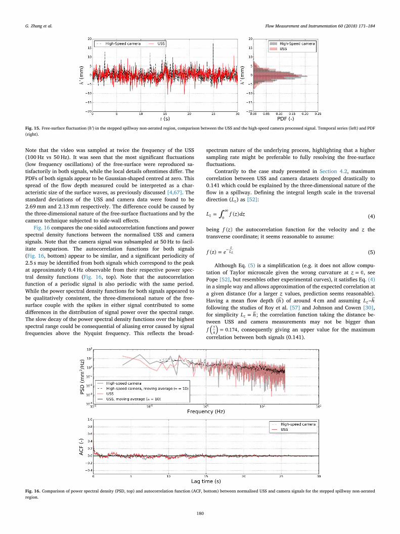
Note that the video was sampled at twice the frequency of the USS(100 Hz vs 50 Hz). It was seen that the most significant fluctuations(low frequency oscillations) of the free-surface were reproduced sa-tisfactorily in both signals, while the local details oftentimes differ. ThePDFs of both signals appear to be Gaussian-shaped centred at zero. Thisspread of the flow depth measured could be interpreted as a char-acteristic size of the surface waves, as previously discussed [4,67]. Thestandard deviations of the USS and camera data were found to be2.69mm and 2.13mm respectively. The difference could be caused bythe three-dimensional nature of the free-surface fluctuations and by thecamera technique subjected to side-wall effects.

Fig. 16 compares the one-sided autocorrelation functions and powerspectral density functions between the normalised USS and camerasignals. Note that the camera signal was subsampled at 50 Hz to facil-itate comparison. The autocorrelation functions for both signals(Fig. 16, bottom) appear to be similar, and a significant periodicity of2.5 s may be identified from both signals which correspond to the peakat approximately 0.4 Hz observable from their respective power spec-tral density functions (Fig. 16, top). Note that the autocorrelationfunction of a periodic signal is also periodic with the same period.While the power spectral density functions for both signals appeared tobe qualitatively consistent, the three-dimensional nature of the free-surface couple with the spikes in either signal contributed to somedifferences in the distribution of signal power over the spectral range.The slow decay of the power spectral density functions over the highestspectral range could be consequential of aliasing error caused by signalfrequencies above the Nyquist frequency. This reflects the broad-

spectrum nature of the underlying process, highlighting that a highersampling rate might be preferable to fully resolving the free-surfacefluctuations.

Contrarily to the case study presented in Section 4.2, maximumcorrelation between USS and camera datasets dropped drastically to0.141 which could be explained by the three-dimensional nature of theflow in a spillway. Defining the integral length scale in the traversaldirection (Lz) as [52]:

∫=∞

L f z dz( )z 0 (4)

being f z( ) the autocorrelation function for the velocity and z thetransverse coordinate; it seems reasonable to assume:

=−f e(z)

zLz (5)

Although Eq. (5) is a simplification (e.g. it does not allow compu-tation of Taylor microscale given the wrong curvature at =z 0, seePope [52], but resembles other experimental curves), it satisfies Eq. (4)in a simple way and allows approximation of the expected correlation ata given distance (for a larger z values, prediction seems reasonable).Having a mean flow depth (h ) of around 4 cm and assuming L h~z

following the studies of Roy et al. [57] and Johnson and Cowen [30],for simplicity =L hz ; the correlation function taking the distance be-tween USS and camera measurements may not be bigger than

=( )f 0.17474 , consequently giving an upper value for the maximum

correlation between both signals (0.141).

Fig. 15. Free-surface fluctuation (h’) in the stepped spillway non-aerated region, comparison between the USS and the high-speed camera processed signal. Temporal series (left) and PDF(right).

Fig. 16. Comparison of power spectral density (PSD, top) and autocorrelation function (ACF, bottom) between normalised USS and camera signals for the stepped spillway non-aeratedregion.

G. Zhang et al. Flow Measurement and Instrumentation 60 (2018) 171–184

180

4.4. Aerated stepped spillway flow

The performance of the USS was further investigated in the fully-developed region on a stepped chute. In this region, the spillway flow ischaracterised by an intense air-entrainment process and strong turbu-lent mixing. The USS has been previously employed by several authorsduring investigations of such type of flows (e.g. [9] at a plungingbreaker; [43,5,72,71] in hydraulic jumps; [67] in smooth spillways;[4,15,66] in stepped spillways). The penetration properties of the ul-trasonic beam in the aerated flow region, however, remain inconclusivebased on several previous reports [35,4,43,5,9], and are likely a com-plex function of the sensor model, beam characteristics and flow con-ditions. Meanwhile, the canonical free-surface is equally ill-defined inthis region. For these reasons, a simple gradient-based technique wasused to extract a characteristic free-surface from the images:

• Construct a gradient image by convolving a Gaussian-blurred ori-ginal image with a Sobel kernel [19];

• Perform a row-wise search to locate a free-surface based on anadaptive threshold;

• Remove any spurious point using a 2D median filter of 39 px indiameter.

Four examples of free-surfaces extracted from the high-speed videocamera images are shown in Fig. 17. The results were reasonably robustdespite the simplistic technique, and the extracted free-surface con-forms generally well to the typical human perception of a free-surface.Note that occasional occurrences of large bright spots due to dropletprojections in the background may result in spurious points unable tobe removed by filtering alone. Such noise will contribute to an in-creased variance in the data, although the likelihood of these events issmall enough that their aggregate effects are deemed to be insignificant.

The USS and camera signals in the aerated flow region are comparedin Fig. 18 (left), and their respective histograms shown in Fig. 18(right). Occasionally, large droplets are projected into the USS deadzone and these data were nulled out by setting a threshold at± 3 timesthe standard deviation of the USS signal. An examination of the wa-veforms indicates some similarities, despite a greater level of variationin the USS data. The histograms shown in Fig. 18 (right) are skewed tothe left (standardized skewness for the data from the camera: -0.40;

USS: -0.59), suggesting a sampling bias towards foreground flow fea-tures (i.e. droplet projection) due to the nature of the pulse-echoprinciple. The standard deviations of the USS and camera data werefound to be 10.79mm and 7.77mm respectively.

The autocorrelation functions and power spectral density functionsof the normalised USS and camera signals are calculated and plotted inFig. 19. Both autocorrelation functions were essentially flat whilelacking any significant periodicities. Correspondingly, the power spec-tral density functions were approximately uniform up to the Nyquistfrequency (25 Hz) similar to that of a white noise. The observationimplies that water surface fluctuations in the aerated flow region en-compasses a broad-spectrum of frequencies, and that the present sam-pling rate was insufficient to adequately resolve the process.

The maximum cross-correlation coefficient between USS andcamera signals was around 0.145, again below the 0.174 approximatedas a theoretical maximum despite the fact that the aerated region ismuch more complex than a normal open channel flow.

4.5. Discussion: USS signal CDF and void fraction profiles

In a free-surface aerated flow, the USS signal outputs provide arange of free-surface locations at a given section. The probability den-sity function (PDF) of the USS signal describes the likelihood of avariable to take a certain value. Similarly, the cumulative densityfunction (CDF) allows knowledge on the probability of that variable toremain below or equal to a given value. When all the air content isentrapped air, the free-surface CDF could be analogous to the time-averaged void fraction profile [67]. However, air bubbles beneath thefree-surface can by no means be accounted with an USS, and this lim-itation must be kept in mind, as this is a common feature of high-ve-locity self-aerated flows [53,54,7,73]. Whereas bubbles cannot be de-tected, capability of the USS to measure the entrapped air wasinvestigated. However, further understanding of the air-water flowstructure is necessary to assess the behaviour of the sensor and, con-sequently, this study only aims to give a glimpse on “what is measured”with an USS when the flow is highly aerated, thus complementing theprevious analysis for non-aerated flows.

In Fig. 20, the void fraction profiles at step edges 4 and 20 areshown, which correspond to sections discussed previously at 0.07mfrom the sidewalls. The theoretical void fraction distributions of

Fig. 17. Free-surface extraction in the aerated flow region. Flow conditions: q =0.110m2/s, θ =26.6°, step 20 (edge). Flow from left to right.

G. Zhang et al. Flow Measurement and Instrumentation 60 (2018) 171–184

181

Chanson and Toombes [12] and Valero and Bung [67] are included inFig. 20 for comparison, and all the data are presented in dimensionlessform in terms of h50 (flow depth where =C 0.5) and with h90 (flowdepth where =C 0.9) obtained with the optical fibre probe, in the non-aerated and the aerated regions respectively, following Zhang andChanson [76].

A number of studies previously associated time-averaged USS datato different void fraction levels [35,4,43,5,9]. In the non-aerated

region, the USS CDF data demonstrated similar accuracy to the opticalfibre probe and theoretical profiles (see Fig. 20 left). In the aerated flowregion, when bubbles are trapped inside the water flow, information onthe void fraction profile are irreparably lost by the USS, as observed inFig. 20 (right). Thereof, capability of the USS to better reproduce thefree-surface roughness will determine up to which extent the entrappedair concentration can be reproduced and, consequently, as entrappedair and entrained air seem to be related [32,65], connection between

Fig. 18. Free-surface fluctuation ( ′h ) in the stepped spillway aerated region, comparison between the USS and the high-speed camera processed signal. Time series (left) and PDF (right).

Fig. 19. Comparison of power spectral density (PSD, top) and autocorrelation function (ACF, bottom) between normalised USS and camera signals for the stepped spillway aeratedregion.

Fig. 20. Air concentration on the non-aerated region (left, step 4) and in the aerated region (right, step 20) measured both with an optical fibre (OF) probe and the USS at 7 cm from thewall.

G. Zhang et al. Flow Measurement and Instrumentation 60 (2018) 171–184

182

USS measurement and total air concentration could be established. USSair concentration profile of Fig. 20 (right) resembles those of Killen [32]obtained with a specific conductivity probe (so-called probabilityprobe). When the air content is predominant ( ≈C 1), the optical fibreand USS measurements converge. The optical fibre and USS data di-verged with decreasing void fraction: for example, the USS reported

≈C 0.6 at =y h/ 190 (OF). Ideally, this was caused by air bubblesforming within the water roughness not being detected by the USS. Themaximum penetration depth of the USS ( = −C 0.02 0.05) correspondedapproximately to =C 0.5 =C(y) 0.5 according to the optical fibre data.This location has been suggested as a transition [51] in the air-waterflow structure [14,17,32,76,8].

5. Conclusion

Ultrasonic sensors (USS) allow dynamic determination of the free-surface which, consequently, allows the estimation of free-surface tur-bulence properties. Herein the applicability of an ultrasonic pulse-echosensor to turbulent free-surface flows was systematically investigated.An examination of the signal characteristics revealed satisfactory fre-quency responses in the sub-20 Hz band, while the signal quality maybe improved by low-pass filtering prior to digitisation. A minimumsampling rate of 50 Hz is recommended in accordance with the sensor’sdynamic capabilities.

The USS performances were tested by sampling synchronously witha Phantom M120 high-speed video camera in several turbulent free-surface flows in order of increasing complexity. The USS is capable ofsatisfactory reproduction of statistics up to the second order when theflow is essentially monophasic and two-dimensional, with dominantmodes in the low frequency range (2D wave flume) (i.e. a 0.25% dif-ference between USS and camera data variance, further to an excellentvisual match). As the water surface fluctuations become more three-dimensional (e.g. high velocity clear water stepped chute flow), the USSis able to reproduce the most energetic modes as long as they are belowthe Nyquist frequency. The sampling bias of the ultrasound beamletstowards foreground signals becomes especially evident when the flowcomprises an inhomogeneous mixture and the free-surface roughness isgoverned by highly three-dimensional processes (e.g. aerated steppedchute flow). In such cases the USS data should be at best interpreted ascharacteristics over the entire sampling surface, on account of its se-verely degraded applicability due to limitations of the sampling prin-ciple.

In highly turbulent flows (e.g. aerated spillway flow), the primarylimitation of the USS is its limited frequency response. The broad-spectrum of time-scales in such processes cannot be adequately resolvedfrom heavily aliased USS signals, and other instrumentations withhigher sample rates are preferable (i.e. phase-detection probes).Applicability of the USS in these cases should be appraised on an in-dividual basis, after a careful validation. Caution should be exercisedwhen the data interpretation extends beyond time-averaged quantities.The USS capabilities to reproduce air transport were tested, showingthat air concentration can be reproduced with similar accuracy to anoptical fibre probe when all the air content is entrapped (i.e. no bubblyflow). In a fully aerated flow, the USS CDF data resembled Killen’s [32]prediction for entrapped air but diverged significantly from the voidfraction distribution determined using an optical fibre probe.

Overall, the present investigation demonstrated the capabilities aswell as limitations of a USS in several types of turbulent flows viasuccessful implementation of a synchronised USS and high-speedcamera sampling system. It is important to note that the individual USSperformance is a complex function of sensor model, surface properties,and flow characteristics, and that actual experimental conditions mightbe more challenging compared to common open channel flows studiedin literature.

Acknowledgements

The authors wish to acknowledge the support of the University ofQueensland Graduate School International Travel Award (UQ-GSITA),of the 2017 Australia-Germany Joint Research Co-operation Scheme(Universities Australia) and the German Academic Exchange Service(DAAD, with financial support of the Federal Ministry of Education andResearch BMBF). The authors also thank A2 Photonic Sensors for pro-viding the optical fibre instrumentation.

References

[1] H.O. Anwar, Discussion on: “self-aerated flows on chutes and spillways”, J.Hydraul. Eng. 120 (6) (1994) 778–779.

[2] B.D. Bissett, Practical Pharmaceutical Laboratory Automation, CRC Press, 2003.[3] D.B. Bung, Developing flow in skimming flow regime on embankment stepped

spillways, J. Hydraul. Res. 49 (5) (2011) 639–648, http://dx.doi.org/10.1080/00221686.2011.584372.

[4] D.B. Bung, Non-intrusive detection of air–water surface roughness in self-aeratedchute flows, J. Hydraul. Res. 51 (3) (2013) 322–329, http://dx.doi.org/10.1080/00221686.2013.777373.

[5] Y. Chachereau, H. Chanson, Free-surface fluctuations and turbulence in hydraulicjumps, Exp. Therm. Fluid Sci. 35 (2011) 896–909, http://dx.doi.org/10.1016/j.expthermflusci.2011.01.009.

[6] K. Chang, G. Constantinescu, Coherent structures in flow over two-dimensionaldunes, Water Resour. Res. 49 (5) (2013) 2446–2460, http://dx.doi.org/10.1002/wrcr.20239.

[7] H. Chanson, Air bubble entrainment in free-surface turbulent shear flows, AcademicPress, 1996.

[8] H. Chanson, Hydraulics of aerated flows: qui pro quo? J. Hydraul. Res. 51 (3)(2013) 223–243, http://dx.doi.org/10.1080/00221686.2013.795917.

[9] H. Chanson, S. Aoki, M. Maruyama, Unsteady air bubble entrainment and de-trainment at a plunging breaker: dominant time scales and similarity of water levelvariations, Coast. Eng. 46 (2) (2002) 139–157, http://dx.doi.org/10.1016/S0378-3839(02)00069-8.

[10] H. Chanson, T. Brattberg, Experimental study of the air–water shear flow in a hy-draulic jump, Int. J. Multiph. Flow. 26 (4) (2000) 583–607, http://dx.doi.org/10.1016/S0301-9322(99)00016-6.

[11] H. Chanson, M. Trevethan, C. Koch, Discussion on turbulence measurements withacoustic Doppler velocimiters, J. Hydraul. Eng. 134 (6) (2007) 883–887, http://dx.doi.org/10.1061/(ASCE)0733-9437(2008)134:6(883).

[12] H. Chanson, L. Toombes, Air-water flows down stepped chutes: turbulence and flowstructure observations, Int. J. Multiph. Flow. 28 (11) (2002) 1737–1761, http://dx.doi.org/10.1016/S0301-9322(02)00089-7.

[13] D. Dabiri, On the interaction of a vertical shear layer with a free surface, J. FluidMech. 480 (2003) 217–232, http://dx.doi.org/10.1017/S0022112002003671.

[14] H. Falvey, Discussion on: bubbles and waves description of self-aerated spillwayflow, J. Hydraul. Res. 45 (1) (2007) 142–144, http://dx.doi.org/10.1080/00221686.2007.9521755.

[15] S. Felder, H. Chanson, Air-water flows and free-surface profiles on a non-uniformstepped chute, J. Hydraul. Res. 52 (2) (2014) 253–263, http://dx.doi.org/10.1080/00221686.2013.841780.

[16] S. Felder, H. Chanson, Phase-detection probe measurements in high-velocity free-surface flows including a discussion of key sampling parameters, Exp. Therm. FluidSci. 61 (2015) 66–78, http://dx.doi.org/10.1016/j.expthermflusci.2014.10.009.

[17] S. Felder, H. Chanson, Air–water flow characteristics in high-velocity free-surfaceflows with 50% void fraction, Int. J. Multiph. Flow. 85 (2016) 186–195, http://dx.doi.org/10.1016/j.ijmultiphaseflow.2016.06.004.

[18] M.M. Gibson, W. Rodi, Simulation of free surface effects on turbulence with aReynolds stress model, J. Hydraul. Res. 27 (2) (1989) 233–244, http://dx.doi.org/10.1080/00221688909499183.

[19] R.C. Gonzalez, R.E. Woods, S.L. Eddins, Digital Image Processing Using MATLAB,Pearson Prentice Hall, 2004 (ISBN: 0-13-008519-7).

[20] C. Gualtieri, P. Gualtieri, Turbulence-based models for gas transfer analysis withchannel shape factor influence, Environ. Fluid Mech. 4 (2004) 249–271.

[21] J.S. Gulliver, M.J. Halverson, Measurements of large streamwise vortices in anopen-channel flow, Water Resour. Res. 23 (1) (1987) 115–123.

[22] X. Guo, L. Shen, Interaction of a deformable free surface with statistically steadyhomogeneous turbulence, J. Fluid Mech. 658 (2010) 33–62, http://dx.doi.org/10.1017/S0022112010001539.

[23] X. Guo, L. Shen, Numerical study of the effect of surface waves on turbulence un-derneath. Part 1. Mean flow and turbulence vorticity, J. Fluid Mech. 733 (2013)558–587, http://dx.doi.org/10.1017/jfm.2013.451.

[24] R.A. Handler, T.F. Swean, R.I. Leighton, J.D. Swearingen, Length scales and theenergy balance for turbulence near a free surface, AIAA J. 31 (11) (1993)1998–2007.

[25] K.V. Horoshenkov, A. Nichols, S.J. Tait, G.A. Maximov, The pattern of surfacewaves in a shallow free surface flow, J. Geophys. Res.: Earth Surf. 118 (3) (2013)1864–1876, http://dx.doi.org/10.1002/jgrf.20117.

[26] K.V. Horoshenkov, T. Van Renterghem, A. Nichols, A. Krynkin, Finite differencetime domain modelling of sound scattering by the dynamically rough surface of aturbulent open channel flow, Appl. Acoust. 110 (2016) 13–22, http://dx.doi.org/

G. Zhang et al. Flow Measurement and Instrumentation 60 (2018) 171–184

183

10.1016/j.apacoust.2016.03.009.[27] T. Hristov, S. Miller, C. Friehe, Dynamical coupling of wind and ocean waves

through wave-induced air flow, Nature 422 (6927) (2003) 55–58, http://dx.doi.org/10.1038/nature01382.

[28] J.C.R. Hunt, J.M.R. Graham, Free-stream turbulence near plane boundaries, J. FluidMech. 84 (2) (1978) 209–235, http://dx.doi.org/10.1017/S0022112078000130.

[29] J. Janssen, The Interaction of Ocean Waves and Wind, Cambridge University Press,2004.

[30] E. Johnson, E. Cowen, Schleiss, et al. (Ed.), Remote Monitoring of VolumetricDischarge based on Surface Mean and Turbulent Metrics. River Flow 2014, Taylor &Francis Group, London, 2014(ISBN 978-1-138-02674-2).

[31] R.I. Karlsson, T.G. Johansson, LDV measurements of higher-order moments of ve-locity fluctuations in a turbulent boundary layer.In: Proceedings of the 3rdInternational Symposium on Applications of Laser Anemometry to FluidMechanics, R.J. Adrian, D.F.G. Durao, F. Durst, H. Mishina, and J.H. Whitelaw(editors), 276-289, 1986.

[32] J.M. Killen, The Surface Characteristics of Self Aerated Flow in Steep Channels(Ph.D. Thesis), University of Minnesota, Minneapolis, MN, 1968.

[33] A. Krynkin, K.V. Horoshenkov, A. Nichols, S.J. Tait, A non-invasive acousticalmethod to measure the mean roughness height of the free surface of a turbulentshallow water flow, Rev. Sci. Instrum. 85 (11) (2014) 114902, http://dx.doi.org/10.1063/1.4901932.

[34] C. Koch, H. Chanson, Turbulence measurements in positive surges and bores, J.Hydraul. Res., IAHR 47 (1) (2009) 29–40, http://dx.doi.org/10.3826/jhr.2009.2954.

[35] S. Kucukali, H. Chanson, Turbulence measurements in the bubbly flow region ofhydraulic jumps, Exp. Therm. Fluid Sci. 33 (1) (2008) 41–53, http://dx.doi.org/10.1016/j.expthermflusci.2008.06.012.

[36] L.D. Landau, E.M. Lifshitz, Fluid Mechanics. Course of Theoretical Physics, secondedition, 6 Elsevier, Butterworth-Heinemann, 1987.

[37] X. Leng, H. Chanson, Unsteady velocity profiling in bores and positive surges, Flow.Meas. Instrum. 54 (2017) 136–145, http://dx.doi.org/10.1016/j.flowmeasinst.2017.01.004.

[38] D. Long, N. Rajaratnam, P.M. Steffler, P.R. Smy, Structure of flow in hydraulicjumps, J. Hydraul. Res. 29 (2) (1991) 207–218, http://dx.doi.org/10.1080/00221689109499004.

[39] J.W. Miles, On the generation of surface waves by shear flows, J. Fluid Mech. 3 (2)(1957) 185–204, http://dx.doi.org/10.1017/S0022112057000567.

[40] M. Mossa, On the oscillating characteristics of hydraulic jumps, J. Hydraul. Res. 37(4) (1999) 541–558, http://dx.doi.org/10.1080/00221686.1999.9628267.

[41] M. Mossa, A. Petrillo, H. Chanson, Tailwater level effects on flow conditions at anabrupt drop, J. Hydraul. Res. 41 (1) (2003) 39–51, http://dx.doi.org/10.1080/00221680309499927.

[42] D. Mouaze, F. Murzyn, J.R. Chaplin, Free surface length scale estimation in hy-draulic jumps, J. Fluids Eng. 127 (2005) 1191–1193.

[43] F. Murzyn, H. Chanson, Free-surface fluctuations in hydraulic jumps: experimentalobservations, Exp. Therm. Fluid Sci. 33 (2009) 1055–1064, http://dx.doi.org/10.1016/j.expthermflusci.2009.06.003.

[44] M. Muste, S. Baranya, R. Tsubaki, D. Kim, H. Ho, H. Tsai, D. Law, Acoustic mappingvelocimetry, Water Resour. Res. 52 (5) (2016) 4132–4150, http://dx.doi.org/10.1002/2015WR018354.

[45] G. Nebbia, Su taluni fenomeni alternativi in correnti libere, L'Energ. Elettr., Fasc. IXIX (1942) 1–10 (in Italian).

[46] I. Nezu, Open-channel flow turbulence and its research prospect in the 21st century,J. Hydraul. Eng. 131 (4) (2005) 229–246, http://dx.doi.org/10.1061/(ASCE)0733-9429(2005)131:4(229).

[47] A. Nichols, S. Tait, K. Horoshenkov, S. Shepherd, A non-invasive airborne wavemonitor, Flow. Meas. Instrum. 34 (2013) 118–126, http://dx.doi.org/10.1016/j.flowmeasinst.2013.09.006.

[48] A. Nichols, S.J. Tait, K.V. Horoshenkov, S.J. Shepherd, A model of the free surfacedynamics of shallow turbulent flows, J. Hydraul. Res. 54 (5) (2016) 516–526,http://dx.doi.org/10.1080/00221686.2016.1176607.

[49] H. Nyquist, Thermal agitation of electric charge in conductors, Phys. Rev. 32 (1)(1928) 110.

[50] A.V. Oppenheim, R.W. Schafer, Discrete-Time Signal Processing, Pearson HigherEducation, 2010.

[51] M. Pfister, Discussion on: bubbles and waves description of self-aerated spillwayflow, J. Hydraul. Res. 46 (3) (2008) 420–423, http://dx.doi.org/10.1080/00221686.2008.9521877.

[52] S. Pope, Turbulent Flows, Cambridge University Press, 2000.[53] N.S.L. Rao, H.E. Kobus, Characteristics of Self-Aerated Free-Surface Flows. Water

and Waste Water/Current Research and Practice 10 Eric Schmidt Verlag, Berlin,Germany, 1971.

[54] N.S.L. Rao, K. Seetharamiah, T. Gangadharaiah, Characteristics of self-aeratedflows, J. Hydraul. Div., ASCE 96 (HY2) (1970) 331–355.

[55] M. Razaz, K. Kawanisi, A. Kaneko, I. Nistor, Application of acoustic tomography toreconstruct the horizontal flow velocity field in a shallow river, Water Resour. Res.51 (12) (2015) 9665–9678, http://dx.doi.org/10.1002/2015WR017102.

[56] V. Roussinova, N. Biswas, R. Balachandar, Revisiting turbulence in smooth uniformopen channel flow, J. Hydraul. Res. 46 (sup1) (2008) 36–48, http://dx.doi.org/10.1080/00221686.2008.9521938.

[57] A.G. Roy, T. Buffin-Bélanger, H. Lamarre, A.D. Kirkbride, Size, shape and dynamicsof large-scale turbulent flow structures in a gravel-bed river, J. Fluid Mech. 500(2004) 1–27, http://dx.doi.org/10.1017/S0022112003006396.

[58] R. Savelsberg, Experiments on Free-surface Turbulence, Technische UniversiteitEindhoven, Eindhoven, 2006, http://dx.doi.org/10.6100/IR609526.

[59] A.B. Schvidchenko, G. Pender, Flume study of the effect of relative depth on theincipient motion of coarse uniform sediments, Water Resour. Res. 36 (2) (2000)619–628 (doi: 0043-1397/00/1999WR900312).

[60] A.B. Schvidchenko, G. Pender, Macroturbulent structure of open-channel flow overgravel beds, Water Resour. Res. 37 (3) (2001) 709–719, http://dx.doi.org/10.1029/2000WR900280.

[61] C.E. Shannon, Communication theory of secrecy systems, Bell Syst. Tech. J. 28 (4)(1949) 656–715.

[62] A. Tamburrino, J.S. Gulliver, Free‐surface visualization of streamwise vortices in achannel flow, Water Resources Research 43 (11) (2007) W11410, http://dx.doi.org/10.1029/2007WR005988.

[63] M.A.C. Teixeira, S.E. Belcher, Dissipation of shear-free turbulence near boundaries,J. Fluid Mech. 422 (2000) 167–191, http://dx.doi.org/10.1017/S002211200000149X.

[64] R.E. Thomas, L. Schindfessel, S.J. McLelland, S. Creëlle, T. De Mulder, Bias in meanvelocities and noise in variances and covariances measured using a multistaticacoustic profiler: the Nortek Vectrino Profiler, Meas. Sci. Technol. 28 (7) (2017),http://dx.doi.org/10.1088/1361-6501/aa7273.

[65] L. Toombes, H. Chanson, Surface waves and roughness in self-aerated supercriticalflow, Environ. Fluid Mech. 7 (3) (2007) 259–270, http://dx.doi.org/10.1007/s10652-007-9022-y.

[66] D. Valero, D.B. Bung, Hybrid Investigations of Air Transport Processes inModerately Sloped Stepped Spillway Flows. In: Proceedings of the 36th IAHR WorldCongress, 28 June–3 July 2015, The Hague, The Netherlands. ISBN: 978-90-824846-0-1, 2015.

[67] D. Valero, D.B. Bung, Development of the interfacial air layer in the non-aeratedregion of high-velocity spillway flows. Instabilities growth, entrapped air and in-fluence on the self-aeration onset. Int. J. Multiph. Flow. 84 (2016) 66–74, http://dx.doi.org/10.1016/j.ijmultiphaseflow.2016.04.012.

[68] D. Valero, D.B. Bung, Reformulating self-aeration: turbulent growth of the freesurface perturbations leading to air entrainment, Int. J. Multiph. Flow. (2017),http://dx.doi.org/10.1016/j.ijmultiphaseflow.2017.12.011.

[69] H. Wang, H. Chanson, Experimental study of turbulent fluctuations in hydraulicjumps, J. Hydraul. Eng. 141 (7) (2015) 04015010, http://dx.doi.org/10.1061/(ASCE)HY.1943-7900.0001010.

[70] H. Wang, H. Chanson, Air entrainment and turbulent fluctuations in hydraulicjumps, Urban Water J. 12 (6) (2015) 502–518, http://dx.doi.org/10.1080/1573062X.2013.847464.

[71] H. Wang, F. Murzyn, Experimental assessment of characteristic turbulent scales intwo-phase flow of hydraulic jump: from bottom to free surface, Environ. FluidMech. (2016) 1–19, http://dx.doi.org/10.1007/s10652-016-9451-6.

[72] H. Wang, F. Murzyn, H. Chanson, Interaction between free-surface, two-phase flowand total pressure in hydraulic jump, Exp. Therm. Fluid Sci. 64 (2015) 30–41,http://dx.doi.org/10.1016/j.expthermflusci.2015.02.003.

[73] I.R. Wood, Air Entrainment in Free-Surface Flows. IAHR Hydraulic StructuresDesign Manual No. 4, Hydraulic Design Considerations, Balkema Publ, Rotterdam,The Netherlands, 1991, p. 149.

[74] W.R. Young, C.L. Wolfe, Generation of surface waves by shear-flow instability, J.Fluid Mech. 739 (2014) 276–307, http://dx.doi.org/10.1017/jfm.2013.617.

[75] G. Zhang, H. Chanson, Hydraulics of the developing flow region of stepped spill-ways. I: physical modeling and boundary layer development, J. Hydraul. Eng. 142(7) (2016) 04016015, http://dx.doi.org/10.1061/(ASCE)HY.1943-7900.0001138.

[76] G. Zhang, H. Chanson, Self-aeration in the rapidly- and gradually-varying flow re-gions of steep smooth and stepped spillways, Environ. Fluid Mech. 17 (2) (2017) 20,http://dx.doi.org/10.1007/s10652-015-9442-z.

[77] Q. Zhong, Q. Chen, H. Wang, D. Li, X. Wang, Statistical analysis of turbulent super-streamwise vortices based on observations of streaky structures near the free sur-face in the smooth open channel flow, Water Resour. Res. 52 (5) (2016) 3563–3578,http://dx.doi.org/10.1002/2015WR017728.

G. Zhang et al. Flow Measurement and Instrumentation 60 (2018) 171–184

184