Multiphase Flow in the Subsurface- Flow of a Light Nonaqueous Phase Liquid

(LNAPL)

Wonyong Jang, Ph.D., P.E.

Multimedia Environmental Simulations Laboratory (MESL)School of Civil and Environmental EngineeringGeorgia Institute of Technology, Atlanta, GA

March 29, 2011

Introduction to Multiphase Flow Multiphase flow means “the simultaneous movement of multiple

phases, such as water, air, non-aqueous phase liquid (NAPL), through porous media.”

Recharge (rain)

UST Gas

Groundwater flowWater

Soil

Atmosphere

Unsaturatedzone

Saturated zone

LNAPL

Pond

Soil (solid)

Water

NAPL contaminant

Gas

Pore-scale soil matrix

Capillary Pressure between Phases Numerical difficulty

• Transition between regions.

Three-phase region:w, n, g

UST

Groundwater flow

Soil

Atmosphere

Two-phaseregion: w, g

Two-phaseregion: w & n

One-phaseregion: w

G

N

W

G

W

N

W

• Two flow equations for water and gas phases

• Two flow equations for water and NAPL phases

• Three flow equations for water, gas and NAPL phases

W, w = waterG, g = gasN, n = NAPL

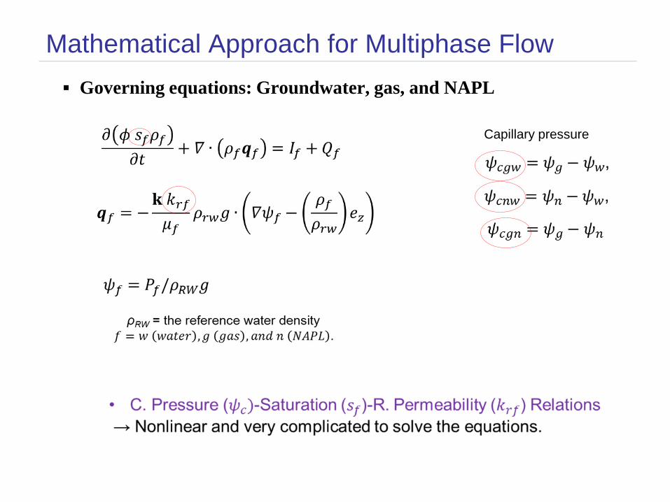
Mathematical Approach for Multiphase Flow Governing equations: Groundwater, gas, and NAPL

Capillary pressure

C. Pressure-Saturation-R. Permeability (1) cP-S-kr relationships

• Brooks-Corey law (1964)

0.1

1.0

10.0

100.0

1000.0

10000.0

100000.0

1000000.0

0 0.1 0.2 0.3 0.4 0.5 0.6 0.7 0.8 0.9 1

Dcnw

or C

apill

ary

Pnw

Effective water saturation

Dcnw

cPnw

Brooks-Corey lawSize index 2Entry Pr. (Pd) 0.5099Residual Sw 0.1Residual Sn 0.1

C. Pressure-Saturation-R. Permeability (2) cP-S-kr relationships

• van Genuchten law (1980)

Three-Phase Systems in the Shallow Aquifer Mobile phases: Water and NAPL Constant pressure head: Gas

• The soil gas in the unsaturated zone is connected to the atmosphere.• The gas movement has negligible impacts on the movement of water and

NAPL.

Water-NAPL Two-Phase System Mobile phases: Water and NAPL No gas phase Example: CO2 injection in deep geological systems

Numerical Techniques Global implicit scheme

• Solves multiphase flow equations simultaneously.• Generates a non-symmetric global matrix.

Upstream weighting scheme (Upwind scheme)• Relative permeability is evaluated based on a flow direction.

Sparse matrix solvers• Iterative matrix solver: IML++

– Failed when the global implicit scheme is used.• Direct matrix solver: Pardiso solver

– Works good with the global implicit scheme.

Buckley-Leverett Problem Buckley-Leverett problem represents a linear water-flood of a

petroleum reservoir in a one-dimensional, horizontal domain. • The pore spaces of the domain is initially filled with a NAPL, i.e., liquid oil.

k = 10-11 m2

Water Qw=AVw

BC Type I for ψwExit boundary for sn

BC Type II for ψwBC Type I for sn

NAPL Qn=AVn

x

sn=0.9, sw=0.1

Properties Values

Boundary condition

Water influx at x=0 mWater pressure at x=300 m

NAPL saturation at x=0 m(Sw at x=0 m)

vw = 0.01 m/s, BC Type IIpw = 2.9 m H2O, BC Type I

sn = 0.1, BC Type I(sw = 0.9, BC Type I)

Initial conditionWater saturationNAPL saturation

sw = 0.1sn = 0.9

Darcy velocity = 0.01 m/s

Properties Values CommentSoil

Intrinsic permeability

Porosity

10-11 m2

0.3

Pore size distribution index 2.0 Brook-Corey law

Water residual saturation

NAPL residual saturation

swr = 0.1

snr = 0.1

FluidWater density

NAPL (oil) density

Water viscosity

NAPL(oil) viscosity

Buckley-Leverett Problem (contd.) Parameters

Buckley-Leverett Problem (Results) Comparison of water saturation profiles

• Semi-analytical solution vs. TechFlowMP results• Coarse and dense meshes

0

0.1

0.2

0.3

0.4

0.5

0.6

0.7

0.8

0.9

1

0 0.1 0.2 0.3 0.4 0.5 0.6 0.7 0.8 0.9 1

Wat

er s

atur

atio

n

Normalized distance (x/L)

AnalySoln

DenseMesh

Coarse Mesh

Domain size, Length

Space step size, SD-A

Space step size, SD-B

L = 5 m

Δx = 0.1 m

Δx = 0.025 m

Coarse grid

Dense grid

Location of the water front

McWhorter-Sunada Problem The flows of water and NAPL are initiated by the capillary pressure

between two phases in a domain.

k = 10-11 m2vw = - vnNo flow boundary

BC Type I for ψw & sw

x=0 m x=2.6 mx

Properties ValuesBoundary condition

Water pressure (x=0 m,t)Water pressure(x=5 m,t)

NAPL saturation (x=0 m,t)(Water saturation (x=0 m,t))NAPL saturation (x=5 m,t)

ψw = 19.885 m H2O, BC Type INo flux/flow boundary

sn = 0., BC Type I(sw = 1., BC Type I)No flow boundary

Initial conditionWater saturation (x, t=0)NAPL saturation (x, t=0)

Water pressure (x, t)

sw = 0.01sn = 0.99

ψw = 19.885 m H2O(Pw =195000 Pa)

McWhorter-Sunada Problem (contd.) Properties Values Remark

SoilSoil intrinsic permeability

Porosity10-11 m2

0.3Pore size distribution index

Entry pressure, Pd

25000 Pa (ψw=0.5099 mH2O)*

Brook-Corey law1 mH2O=9806.65Pa

Water residual saturation NAPL residual saturation

swr = 0.snr = 0.

FluidWater density

NAPL (oil) densityWater viscosity

NAPL(oil) viscosity

ρw = 1000 kg/m3

ρn = 1000 kg/m3

0.001 Pa s-1 (= kg/m s)0.001 Pa s-1 (= kg/m s)

Domain and space discretizationDomain size, Length

Space step sizeL = 2.6 m

Δx = 0.01 m 260 elements

Water viscosityNAPL(oil) viscosity

0.001 Pa s-1 (= kg/m s)0.001 Pa s-1 (= kg/m s)

Time discretizationSimulation timeTime step size

T = 10,000 sΔt = 1 – 100 s (Max. 15 iterations)

McWhorter-Sunada Problem (contd.) The change in water saturation over time

• Semi-analytical solutions vs. TechFlowMP results– The global implicit scheme, upwind scheme, and Pardiso solver are

implemented.

0.0

0.1

0.2

0.3

0.4

0.5

0.6

0.7

0.8

0.9

1.0

0.0 0.5 1.0 1.5 2.0 2.5 3.0

Wat

er

Satu

rati

oo

n

X (m)

AS@1000s

AS@4000s

AS@10000s

TF1000s

TF4000s

TF10000s

NAPL Release at the Ground Surface NAPL’s release into the variably saturated zone.

• Three phases: water, gas, and NAPL.• A NAPL is released for 600 sec.

k = 9.9 10-12 m2

z=1 ft(0.3m)dz=0.05ft

Constant atmospheric pressure

z

NAPL source,Qn=0.505 ft3/d for 600 sec

BC Type I for ψw

x= 3.05ft (0.9 m)dx=0.18ft (0.055m)

z=0.4 ft

x

Initial condition

• Water: Variable sw• NAPL: sn = 0 at t=0 sec• Water head: ψw = 0.4 ft H2O

Domain and space discretization

• X = 93 cm: Δx = 0.18 ft (5.47 cm)• Z = 30.48 cm: Δz = 0.05 ft (1.524 cm)

Time discretization

• Simulation time: T = 10 hrs (Δt = 0.01 – 8 sec)

NAPL Release at the Ground Surface (contd.)NAPL’s spreading with time.

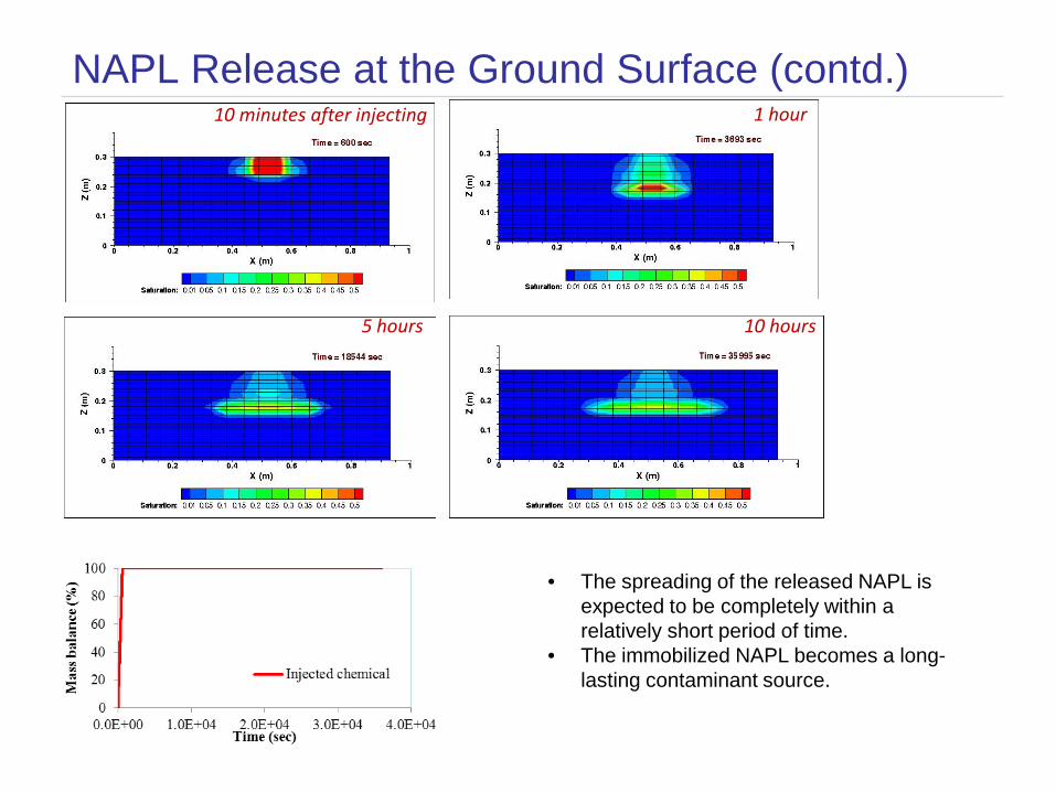
NAPL Release at the Ground Surface (contd.)

• The spreading of the released NAPL is expected to be completely within a relatively short period of time.

• The immobilized NAPL becomes a long-lasting contaminant source.

10 minutes after injecting 1 hour

5 hours 10 hours

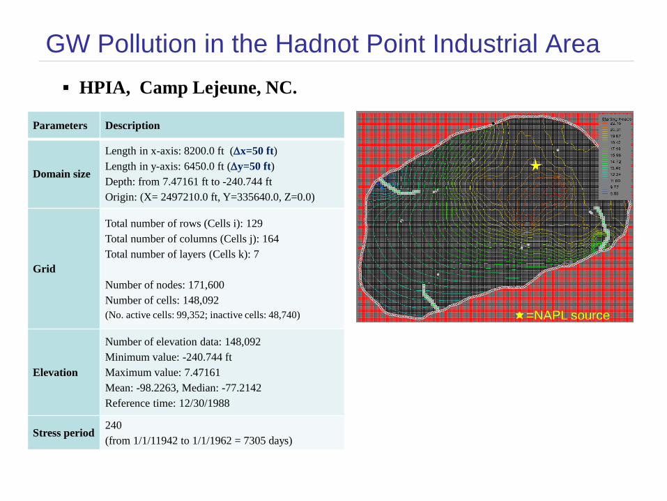
GW Pollution in the Hadnot Point Industrial Area HPIA, Camp Lejeune, NC.

Parameters Description

Domain size

Length in x-axis: 8200.0 ft (∆x=50 ft)Length in y-axis: 6450.0 ft (∆y=50 ft)Depth: from 7.47161 ft to -240.744 ftOrigin: (X= 2497210.0 ft, Y=335640.0, Z=0.0)

Grid

Total number of rows (Cells i): 129Total number of columns (Cells j): 164Total number of layers (Cells k): 7

Number of nodes: 171,600 Number of cells: 148,092 (No. active cells: 99,352; inactive cells: 48,740)

Elevation

Number of elevation data: 148,092Minimum value: -240.744 ftMaximum value: 7.47161Mean: -98.2263, Median: -77.2142Reference time: 12/30/1988

Stress period240 (from 1/1/11942 to 1/1/1962 = 7305 days)

=NAPL source

Application to GW Pollution in HPIA (contd.) NAPL at HPIA, Camp Lejeune, NC.

• Contaminant sources are immobilized NAPLs. • The dissolution of the immobile NAPL and its

transport in the whole domain will be investigated.

• The migration of the NAPL can be analyzed within a very limited region around the source area.

Thank you.

Questions?

References• Brooks, R.H. and Corey, A.T., 1964. Hydraulic Properties of Porous Media. Hydrology Paper 3., 27 pp., Colorado

State University, Fort Collins, Co.• Helmig, R., 1997. Multiphase flow and transport processes in the subsurface : a contribution to the modeling of

hydrosystems. Environmental engineering. Springer, Berlin ; New York, xvi, 367 p. pp.• van Genuchten, M.T., 1980. A closed-form equation for predicting the hydraulic conductivity of unsaturated soils.

Soil Science Society of America Journal, 44(5): 892-898.