Purdue UniversityPurdue e-Pubs

CTRC Research Publications Cooling Technologies Research Center

2012

Flow Regime-Based Modeling of Heat Transfer andPressure Drop in Microchannel Flow BoilingT. HarirchianPurdue University

S. V. GarimellaPurdue University, sureshg@purdue.edu

Follow this and additional works at: http://docs.lib.purdue.edu/coolingpubs

This document has been made available through Purdue e-Pubs, a service of the Purdue University Libraries. Please contact epubs@purdue.edu foradditional information.

Harirchian, T. and Garimella, S. V., "Flow Regime-Based Modeling of Heat Transfer and Pressure Drop in Microchannel Flow Boiling"(2012). CTRC Research Publications. Paper 173.http://dx.doi.org/10.1016/j.ijheatmasstransfer.2011.09.024

1

Flow Regime-Based Modeling of Heat Transfer and Pressure Drop in

Microchannel Flow Boiling

Tannaz Harirchian and Suresh V. Garimella1

School of Mechanical Engineering and Birck Nanotechnology Center

585 Purdue Mall, Purdue University

West Lafayette, IN 47907-2088 USA

ABSTRACT

Local heat transfer coefficients and pressure drops during boiling of the dielectric liquid fluorinert

FC-77 in parallel microchannels were experimentally investigated in recent work by the authors. Detailed

visualizations of the corresponding two-phase flow regimes were performed as a function of a wide range

of operational and geometric parameters. A new transition criterion was developed for the delineation of

a regime where microscale effects become important to the boiling process and a conventional,

macroscale treatment becomes inadequate. A comprehensive flow regime map was developed for a wide

range of channel dimensions and experimental conditions, and consisted of four distinct regions – bubbly,

slug, confined annular, and alternating churn/annular/wispy-annular flow regimes. In the present work,

physics-based analyses of local heat transfer in each of the four regimes of the comprehensive map are

formulated. Flow regime-based models for prediction of heat transfer coefficient in slug flow and

annular/wispy-annular flow are developed and compared to the experimental data. Also, a regime-based

prediction of pressure drop in microchannels is presented by computing the pressure drop during each

flow regime that occurs along the microchannel length. The results of this study reveal the promise of

flow regime-based modeling efforts for predicting heat transfer and pressure drop in microchannel

boiling.

Keywords: microchannel flow boiling, regime-based modeling, flow map, heat transfer, pressure drop

1 Author to whom correspondence should be addressed: (765) 494-5621, sureshg@purdue.edu

2

NOMENCLATURE

cA vapor core cross-sectional area

( 2 2c ch chA w d )

csA cross-sectional area of a microchannel, mm2

fA wetted area of a fin, m2

manA cross-sectional are of outlet manifold

plA cross-sectional are of entrance plenum

tA total heated/wetted area of all microchannels

in a heat sink, m2

Bl boiling number ( Bl q

w/ Gh

fg)

Bo Bond number ( 2( ) /f gBo g D )

C liquid droplet concentration

Ca Capillary number ( /fCa u )

fic correction factor for interfacial friction

factor

pc specific heat of the fluid

qc empirical parameter in Eq. (42)

0C correction factor for initial film thickness in

slug flow

chd microchannel depth, m

D length scale ( csA ), m

hD hydraulic diameter, μm

hHD hydraulic diameter based on the heated

perimeter ( cshH

H

AD

P ), m

0e liquid droplet quality

f friction factor

g gravitational acceleration

G mass flux, kg m-2

s-1

h heat transfer coefficient, W m-2

K-1

fgh latent heat of vaporization for FC-77, J kg-1

j superficial velocity, m s-1

cK contraction coefficient

dk deposition mass transfer coefficient

k thermal conductivity, W m-1

K-1

L length, m

0aL location of annular flow incipience along the

channel length, m

HL axial heated length, m

m used in fin efficiency calculation

( 2 si fm h k w ) , m-1

fgm evaporation mass flux

m mass flow rate, kg s-1

M molecular mass of the fluid

N number of microchannels in a test piece

fn empirical parameter in Eq. (42)

pchN phase change number

qn empirical parameter in Eq. (42)

P pressure

cP vapor core perimeter

( 2 2 2c ch chP w d ), m

chP channel perimeter ( 2ch ch chP w d )

HP heated perimeter ( 2H ch chP w d ), m

rp reduced pressure

wq wall heat flux, W m-2

Re Reynolds number ( Re GD / )

hRe Reynolds number ( Re /hGD )

pR surface roughness parameter

3

T temperature, ºC

refT reference temperature: fT in single-phase

region and satT in two-phase region, ºC

u velocity, m s-1

chw microchannel width, m

fw microchannel fin width, m

We Weber number ( 2 /h fWe G D )

x vapor quality

0x vapor quality at the onset of annular flow

exitx vapor quality at microchannel exit

vvX Martinelli parameter

y distance from the channel wall

z direction along the channel length ?????

Greek symbols

microchannel aspect ratio

liquid film thickness

P pressure drop

d deposition mass transfer rate per unit length,

kg m-1

s-1

fg evaporation mass transfer rate per unit

length, kg m-1

s-1

density, kg m-3

dynamic viscosity, kg m-1

s-1

surface tension, N m-1

f efficiency of a fin in the microchannel heat

sink ( tanh chf

ch

md

md )

o overall surface efficiency of the

microchannel heat sink ( 1 1f

o f

t

NA

A )

fluid particle residence time, s; shear stress;

period of slug flow

frequency of vapor generation, s-1

Subscripts

0 initial

a annular flow

c contraction; vapor core

ch channel

dev developing flow

dry vapor slug region in slug flow

e expansion

E entrained liquid droplets in annular flow

vapor core

f liquid; liquid slug

fd fully developed

film liquid film in annular/wispy-annular flow;

elongated bubble region in slug flow

g vapor

H homogeneous

i interfacial

in inlet

meas measured

p liquid slug and bubble pair in slug flow

s slug flow

sat saturated liquid

si silicon

sp single-phase

w microchannel wall

1. INTRODUCTION

Boiling and two-phase flow in microchannels have been investigated extensively in the literature for

the past decade. The primary motivation for this work has been the high heat flux handling capability of

4

microchannel heat sinks undergoing boiling while maintaining minimal temperature gradients over the

heated surface. Experimental studies in the literature have focused on characterizing the heat transfer

performance and pressure drop, flow patterns, flow instabilities, and critical heat flux; a variety of

predictive correlations for heat transfer and pressure drop have also been proposed as reviewed in

Garimella and Sobhan [1], Thome [2], and Bertsch et al. [3].

In recent work by the authors [4, 5], flow boiling experiments were conducted in microchannels with

a perfluorinated dielectric liquid, FC-77, and the effects of heat flux, mass flux, and channel dimensions

on heat transfer and pressure drop in microchannel boiling were studied. A wide range of microchannel

widths from 100 µm to 5850 µm with depths of 100 µm to 400 µm, were studied. The mass flux and heat

flux values ranged from 225 to 1420 kg/m2s and from 25 to 380 kW/m

2, respectively. Figure 1 shows a

photograph of the test setup used to perform these experiments. In Harirchian and Garimella [6], a new

transition criterion was proposed for delineating microchannel behavior from that of macrochannels,

based on the occurrence of flow confinement due to the microchannel walls. Flow visualizations [7]

showed that the flow velocity affects the bubble diameter and hence the confinement effects, and

therefore, the existence of microscale effects depend not only on the channel size and fluid properties, but

also on the flow velocity. This new transition criterion to define the conditions under which a channel

behaves as a microchannel was formulated in terms of the Bond number and Reynolds number and was

termed the convective confinement number; 0.5 160Bo Re defines this transition between micro- and

macro-channels, with values smaller than 160 corresponding to microchannels.

Bar-Cohen and Rahim [8] examined the predictions from five classical two-phase heat transfer

correlations for mini-channel flow. They concluded that although some of these correlations provide

good accuracy in the prediction of single-channel refrigerant flow, they fail to predict boiling of water in

single microchannels or of refrigerants and dielectric liquids in multiple microchannel configurations.

Harirchian and Garimella [4] compared their experimental results for boiling of FC-77 in microchannels

with predictions from 10 empirical correlations developed for convective flow in macrochannels and

microchannels as well as for pool boiling, and showed that none of the examined correlations predicted

the measurements adequately. The best agreement was obtained with the pool boiling correlation of

Cooper [9]. In a comprehensive review by Bertsch et al. [3], predictions from 25 widely used correlations

for boiling heat transfer coefficient were compared against a large database of 1847 data points from ten

different published studies in the literature. This effort also showed that the pool boiling correlation of

Cooper [9] provided the best overall match; more generally, this comprehensive quantitative comparison

showed that the pool boiling correlations evaluated resulted in a better prediction of the microchannel

flow boiling data than those proposed particularly for flow boiling, and that nucleate boiling dominates

the heat transfer in microchannels. Among all the correlations assessed by Bertsch et al. [3], only one

was developed based on the prevalent flow regime [10]; however, only a single flow regime of slug flow

5

was considered in Thome et al. [10]. Bertsch et al. [3] pointed to a clear need for the development of

physics-based models based on the prevalent flow regimes to predict microchannel flow boiling.

Few regime-based models exist in the literature for the prediction of heat transfer coefficient and

pressure drop in microchannel flow boiling. Thome et al. [10] proposed a three-zone boiling model to

predict the local dynamic and time-averaged heat transfer coefficient in the elongated bubble regime.

This model assumed the passage of a liquid slug, confined elongated bubble, and vapor slug at a fixed

point in the microchannel, with transient evaporation of the thin liquid film surrounding the elongated

bubble being the dominant heat transfer mechanism (rather than nucleate boiling). This model illustrates

the strong dependency of the heat transfer on bubble frequency, the minimum liquid film thickness at

dryout, and the liquid film formation thickness, all of which are obtained from experiments due to the

difficulty in obtaining them theoretically. The authors compared the time-averaged local heat transfer

coefficient predicted by the three-zone model to the experimental measurements from seven independent

studies in the literature, including six refrigerants and CO2 [11], and obtained a set of general empirical

parameters to be used in the model. The model predicted 67% of the database within a mean average

error (MAE) of ±30%. Ribatski et al. [12] compared predictions from the three-zone slug flow model

[10] to experimental results for boiling heat transfer of pure Acetone. Using the general empirical

parameters developed in [11], 69% of the experimental data were predicted to within ±30%, while using a

new set of empirical parameters optimized for Acetone data, the model predicted 90% of the heat transfer

data to within ±30%. Predictions from this model were also compared to experimental data for flow

boiling of R254fa and R236fa [13]. Adjusting the empirical parameters of the model to this experimental

dataset, the model predicted 90% of the measurements to within ±30% of error. Shiferaw et al. [14]

compared their experimental data with R134a to the predictions from the three-zone model of Thome et

al. [10] as well as from other empirical correlations and suggested that the three-zone model based on

convective heat transfer performs at least as well as empirical correlations that interpret the data in terms

of nucleate boiling.

Qu and Mudawar [15] performed experiments in water-cooled microchannel heat sinks and showed

an abrupt transition to an annular regime upon the onset of boiling. They concluded that the dominant

heat transfer mechanism in microchannels is forced convective boiling corresponding to annular flow.

Comparison of their experimental results to predictions from 11 empirical correlations which were

developed for both macrochannels and microchannels revealed deviations from 19.3% to 272.1% in terms

of mean absolute errors due to the unique features of water-cooled microchannel boiling and the operating

conditions that fall outside the recommended range for most correlations. Qu and Mudawar [16]

developed a model to predict the saturated heat transfer coefficient in the annular regime, incorporating

features relevant to boiling of water in microchannels such as laminar liquid and vapor flow, smooth

interface, and strong droplet entrainment and deposition effects. Their model predicted their experiments

with an MAE of 13.3%. Their model also allowed the calculation of pressure drop over the length of the

6

annular region, considering the entire two-phase length of the channel as being in annular flow [17]. This

led to an MAE of 12.7%, matching the accuracy of the best of ten empirical correlations that were also

tested.

Quiben and Thome [18] performed an analytical investigation of pressure drop during boiling in

horizontal single tubes. They proposed a flow pattern-based model for prediction of the frictional

pressure drop, treating each flow regime separately and assuming that only one flow regime exists in the

complete test section. Their model ensured a smooth transition in the predicted pressure drop at the

transitions between flow regimes and predicted 82.3% of the experimental data with three refrigerants

[19] to within ±30%.

A review of the literature reveals only a few studies that have focused on modeling of flow boiling

based on the existing flow regimes and taken into account the interfacial structure between the liquid and

vapor phases. Also, even these studies have assumed the existence of a single regime in the channels. It

has been shown in the literature [7, 20-23], however, that different flow regimes can be present in

microchannels under different operational and geometric conditions, or even in a single microchannel

along its length. One such study is the recent detailed experimental investigation by the authors [7],

where five different flow regimes were observed for boiling of FC-77 in microchannels over a wide range

of channel dimensions. In their later study [6], it was shown that for convective confinement numbers

smaller than 160 (i.e., 0.5 160Bo Re ), vapor bubbles are confined within the channel walls and

convective boiling is the dominant heat transfer mechanism. Two flow regimes of slug flow and confined

annular flow were visualized along the channels under such confined conditions. For larger convective

confinement numbers, however, bubbly flow and alternating churn/annular and alternating churn/wispy-

annular flow were observed with nucleate boiling being dominant.

To develop flow-regime based models for heat transfer coefficient and pressure drop, it is essential

that flow regime maps be available along with quantitative criteria for flow pattern transitions to

determine the flow pattern that exists under a given set of conditions. Such a comprehensive flow regime

map was developed for boiling of FC-77 in Harirchian and Garimella [6], using nondimensional

parameters of Bl Re and 0.5Bo Re as the coordinates. Using these coordinates, four quadrants

representing flow regimes of slug, confined annular, bubbly, and alternating churn/annular/wispy-annular

flow were identified on the map. In the present study, a modified version of this flow regime map is

presented with the phase change number and convective confinement number as the coordinates, which

enables the determination of the location along the microchannels where the transition between different

flow regimes occurs.

In the present study, the three-zone model of Thome et al. [10] for slug flow is examined against the

measured data in the slug region. The model is then modified by using a different method for prediction

of the initial liquid film thickness surrounding the elongated bubble in order to improve the original

model for better agreement with the measurements. For the annular flow regime, an analytical model is

7

developed to predict local heat transfer coefficient. An empirical parameter is introduced for calculating

the interfacial shear stress in the liquid film surrounding the vapor core. This model also enables

calculation of pressure drop in the annular flow.

Although pressure drop in the annular region can be predicted with the annular heat transfer model

proposed in this study, calculation of pressure drop across the full length of the channel is more complex

due to the existence of several regimes along the channels. Two different treatments are therefore

proposed for the confined flow and the unconfined flow regimes to calculate the total pressure drop in the

microchannels. Also, six widely used empirical correlations from the literature are examined. It is shown

that the regime-based approach in the current work to calculate the pressure drop predicts the

experimental data much better than any of the tested empirical correlations. The importance of a

knowledge of the exact location where a flow regime transition occurs is discussed, as are means to

improve the pressure drop predictions.

2. NEW COMPREHENSIVE FLOW REGIME MAP

The experimental investigation of flow boiling in parallel silicon microchannels with the

perfluorinated fluid FC-77 by Harirchian and Garimella [4, 5] considered 12 different test pieces

incorporating rectangular microchannels of different cross-sectional dimensions tested over a wide range

of heat fluxes and mass flow rates; a database with approximately 390 data points was obtained. Table 1

lists the width, depth, number of channels in each heat sink, and surface roughness along with the mass

fluxes tested. For each test piece, the mass flux and fluid temperature at the inlet of the microchannels

were fixed and the heat flux was incremented from zero to a maximum value limited by the upper

temperature limit (150ºC) for the safe operation of the test chips. Twenty five embedded resistor heat

sources fabricated on the underside of the silicon test piece provided a uniform heat flux to the base of the

microchannels, while 25 temperature-sensing diodes facilitated local measurement of the base

temperature, and thus, a local calculation of the heat transfer coefficient. High-speed visualizations were

simultaneously performed to obtain detailed videos of the flow boiling regimes inside the channels for

each set of conditions. More information on the test chip fabrication, test section assembly, sensor

calibration, test procedure, and data reduction is available in Harirchian and Garimella [4, 5] and hence

not repeated here.

Based on the experimental results and flow visualizations obtained in Harirchian and Garimella [5, 7]

for flow boiling in microchannels, a comprehensive flow regime map was developed in Harirchian and

Garimella [6]. The convective confinement number, 0.5Bo Re , and a nondimensional form of heat flux,

Bl Re , were used as the abscissa and the ordinate of this map, respectively, and quantitative transition

criteria were proposed. This flow regime map was developed for flow regimes occurring at a specific

location along the length of the microchannel heat sink where the heat transfer measurements were

obtained (1.27 mm short of the exit of the central channel). It is noted that the length scale used in the

8

Reynolds number, /Re GD , and the Bond number, 2( ) /f gBo g D , is the square root of

the microchannel cross-sectional area, csD A , as discussed in Harirchian and Garimella [6].

The flow regime map developed in Harirchian and Garimella [6] is modified here to include the effect

of the heated length of the microchannels on two-phase flow development by using the phase change

number as the ordinate in the map. The phase change number was first introduced by Saha et al. [24] to

represent the rate of phase change due to heat addition and is defined as

pchN (1)

where f gw H

cs fg f g

q P

A h

is the frequency of vapor generation and

/

H H

f

L L

u G

is the fluid

particle residence time. Hence the phase change number can be rewritten as

/

f g f gw H H Hpch

cs fg f g f hH g

q P L LN Bl

A h G D

(2)

Using the phase change number, pchN , and the convective confinement number, 0.5Bo Re , as

coordinates, the flow regime map in Figure 2 is obtained. Unlike the flow regime map developed in

Harirchian and Garimella [6], this map includes data from five different locations along the microchannel

length at which simultaneous local heat transfer measurements and local flow visualizations were

performed. As in the previous comprehensive map, a wide range of microchannel dimensions, heat

fluxes, and mass fluxes is included in this map. The transition lines divide the map into four distinct

quadrants of slug and confined annular flow for 0.5 160Bo Re and bubbly and alternating

churn/annular and churn/wispy-annular for larger convective confinement numbers.

The vertical transition line on the map represents the transition from confined flow, where microscale

effects are present and convective boiling is the dominant heat transfer mechanism, to unconfined flow

with nucleate boiling being dominant, and is expressed as

0.5 160Bo Re (3)

The other transition line is a curve fit to the points of transition from bubbly or slug flow to alternating

churn/annular or churn/wispy annular flow and is given by

0.258

0.596.65pchN Bo Re

(4)

Substituting Eq. (2) in Eq. (4), the location along the microchannels at which the transition from bubbly

or slug to annular flow occurs can be determined from

0.258

0.5 1

0 96.65g cs

a

f g H

AL Bo Re Bl

P

(5)

0aL is used in modeling of the heat transfer coefficient and pressure drop in the annular flow regime, as

will be discussed in section 4.2.1. This new comprehensive map reveals that although annular and wispy-

9

annular regimes may exist near the exit of the microchannels under specific test conditions, a large

portion of the microchannels may experience bubbly or slug flow regimes; hence, an assumption of the

presence of a single flow pattern in the microchannels is incorrect for the boiling of perfluorinated liquids,

especially when a wide range of parameters is considered.

3. EMPIRICAL CORRELATIONS

A large number of empirical correlations have been developed in various studies in the literature for

prediction of heat transfer and pressure drop in flow boiling in microchannels as recently reviewed by

Bertsch et al. [3]. Harirchian and Garimella [4] compared their experimental heat transfer coefficients to

predictions from ten correlations from the literature. Four of these correlations were developed for

channels of conventional sizes [25-28], four were developed for microchannels [29-32], and two are

widely used correlations for pool boiling [9, 33]. The experiments of Harirchian and Garimella [4] were

also compared by Bertsch et al. [3] to 15 other empirical correlations [10, 34-47] for flow boiling in small

and large channels. It is noted that the experimental local heat transfer coefficient was calculated [4]

using the locally measured wall temperature and the local wall heat flux, wq , which is evaluated based on

the total heated area of the microchannel

w

o w ref

qh

T T

(6)

The values of mean average error along with the percentage of data predicted within ±30% for all of

the 25 correlations used in the comparisons [3, 4] are listed in Table 2; the fluid and geometry considered

in the development of each correlation is also listed. As seen in this table and concluded by Bertsch et al.

[3] and Harirchian and Garimella [4], none of the examined correlations predict the heat transfer

measurements adequately, except Cooper’s pool boiling correlation [9] which predicts the experimental

results with MAE of 11.9%.

The experimental results for pressure drop are also compared in this study with predictions from

empirical correlations in the literature. In the experiments [4, 5], the pressure drop measured between the

inlet and outlet manifolds located upstream and downstream of the microchannels ( measP ) includes the

pressure drop across the microchannels and the inlet and outlet manifolds as well as the pressure loss

( cP ) and recovery ( eP ) due to the inlet contraction and the outlet expansion. For the cases considered

in this study, the contraction pressure loss and expansion pressure recovery can constitute up to 15% and

1% of the total measured pressure drop, respectively; however, the pressure drop in the inlet and outlet

manifolds accounts for less than 0.06% of the total measured pressured drop, and hence, is neglected in

the microchannel pressure drop calculations. Therefore, the pressure drop across the microchannels alone

is extracted as follows:

ch meas e cP P P P (7)

10

The flow contraction occurs at two cross-sections downstream of the inlet manifold: first, at the

entrance to a plenum that connects the inlet manifold to the microchannels, and second, at the entrance to

the microchannels. The working fluid enters the microchannels in a purely liquid state. The pressure loss

associated with the flow contraction at the inlet of the microchannels is obtained from [48, 49]

221

12

csc c

pl f

NA GP K

A

(8)

Here, cK is the contraction coefficient given by

20.0088 0.1785 1.6027cK (9)

The pressure loss at the entrance of the connecting plenum is calculated similarly, using the appropriate

values for the cross-sectional areas and mass flux in Eq. (8) and aspect ratio in Eq. (9).

A two-phase mixture of liquid and vapor exits the microchannels and the pressure recovery resulting

from the flow expansion at the exit for two-phase flow is calculated from [50]

2

2

, 2

5 11 1 1cs cs

e tp exit

f man man vv vv

NA NAGP x

A A X X

(10)

in which vvX is the Martinelli parameter for laminar liquid and laminar vapor phases and is given by

0.5 0.50.5

1f gexit

vv

g exit f

xX

x

(11)

The corrected value of chP so obtained is compared to predicted values. In cases where both single-

phase and two-phase flow exists in the microchannels, the predicted values are calculated separately for

the single-phase and two-phase regions. The single-phase pressure drop is calculated using the approach

of Lee and Garimella [47]. The single-phase region in the microchannels can be divided into a

developing and a fully developed region for which the lengths can be obtained from [47]

,

if 0.05

0.05 if 0.05

sp sp

sp dev

h h sp

L LL

Re D L

(12)

, ,sp fd sp sp devL L L (13)

where /sp sp h hL L Re D , hRe is the Reynolds number calculated using the channel hydraulic

diameter, and spL is the overall single-phase region length, which can be obtained from a heat balance

,cs p sat f in

sp

w H

GA c T TL

q P

(14)

The friction factor associated with the developing region is then obtained from

11

0.052

0.57 2

,0.05

2 20.57

3.2 / 0.5 / if 0.05

3.2 / 0.5 0.05 / if 0.05

sp fd h h sp

sp dev

fd h h sp

L f Re Re L

f

f Re Re L

(15)

where the fully developed friction constant for a rectangular channel is

2 3 4 596 / 1 1.3553/ 1.9467 / 1.7012 / 0.9564 / 0.2537 /fd hf Re (16)

The total single-phase pressure drop in then obtained from

2

, , , ,

2

sp dev sp dev sp fd sp fd

sp

f h

f L f LGP

D

(17)

The pressure drop in the two-phase region of the microchannels is the sum of the frictional and the

accelerational components. A large number of empirical correlations are available in the literature for

prediction of these two components and many studies in the literature have compared these correlations to

experimental data [17, 44, 47, 51, 52]. Six of these correlations that predicted the experiments of Qu and

Mudawar [17], Lee and Mudawar [44], and Lee and Garimella [47] better than other correlations are

chosen here for comparison to the experimental data. One of these correlations is a widely used

macrochannel correlation [53], while the others were developed for mini/microchannels [17, 40, 44, 47,

54]. Predictions from these correlations are compared with the measured pressure drops in Figure 3. The

MAEs listed in this figure ranging from 84.7% to 394.2% reveal the failure of these empirical correlations

in providing a suitable prediction of the experimental results, mainly because the correlations were

developed for specific fluids and ranges of operating parameters that differ from those of the current

experimental data.

Although the pool boiling correlation of Cooper was shown to predict the experimental heat transfer

data well, none of the empirical correlations developed specifically for flow boiling in microchannels

were found to predict experimental heat transfer coefficient and pressure drop to within a reasonable

error. Hence, it is essential to develop physics-based models based on the relevant flow regimes to

predict both heat transfer coefficient and pressure drop in microchannel flow boiling. Physics-based

models are expected to be applicable to a wider range of parameters, and not just to specific data sets.

4. MODEL DEVELOPMENT

It was shown in the previous section that existing pressure drop correlations in the literature fail to

provide acceptable predictions of the current experimental data. For prediction of the heat transfer

coefficient, only the pool boiling correlation of Cooper [9] was shown to predict the results well (with an

MAE of 11.9%). The ability of the Cooper correlation to predict flow boiling heat transfer has been

pointed out in other studies in the literature as well, for cases where nucleate boiling is the dominant heat

transfer mechanism. However, in many practical applications, microchannels undergo confined flow

12

where convective boiling is dominant and the Cooper correlation, originally developed for nucleate

boiling, does not perform as well (as observed by the increase in the errors in prediction for slug and

confined annular flows with MAE of 15.3% and 14.5%, respectively). In addition, this correlation does

not provide any information regarding the pressure drop.

In this section, three different analytical models are proposed for three of the four quadrants of the

flow regime map in Figure 2, i.e., confined annular, annular/wispy-annular, and slug flow. The three

models are then validated by a comparison to the experimental data. For the fourth region of bubbly flow,

use of the Cooper [9] correlation is suggested. In conjunction with the transition criteria proposed in

section 2, the consistent physics-based models developed for heat transfer are also capable of predicting

the pressure drop in the microchannels. It will be seen in the following subsections that the models

developed for slug flow and confined annular flow predict the experimental heat transfer data with

accuracy similar to that of the Cooper correlation; moreover, the pressure drop predictions using the

proposed physical models are far more accurate than the existing correlations.

4.1. Bubbly flow

An analytical model for the bubbly flow is not attempted in this study since it has been shown

previously [3, 4] that the empirical correlation of Cooper [9] for pool boiling predicts the experimental

data very well in this nucleate boiling dominant region. This correlation is given by

0.550.12 0.4343ln 0.5 0.6755 0.4343lnpR

r r wh p p M q (18)

Figure 4 depicts predictions from Cooper’s pool boiling correlation for the bubbly flow data in the

current study; the MAE is 13.9% and 86.5% data points are captured to within 30%.

4.2. Confined annular flow

A model for prediction of heat transfer coefficient and pressure drop in confined annular flow in

microchannels with a rectangular cross-section is developed based on the conservation of mass,

momentum, and energy, using an approach similar to that presented by Carey [55] for large vertical tubes

of circular cross-section.

4.2.1 Model development

Figure 5(a) shows a schematic representation of annular flow in microchannels. A continuous vapor

core flows along the center of the microchannel and is surrounded by a thin liquid film along the channel

walls. Liquid droplets can be entrained into this vapor core. The model discussed here assumes that the

two-phase flow is steady, the pressure is uniform across the channel cross-section, the vapor quality in the

annular flow region is equal to the thermodynamic equilibrium quality, the liquid film-vapor core

interface is smooth, and the thickness of the liquid film is uniform along the channel circumference. Also,

13

it is assumed that droplet deposition is uniform along the channel perimeter, and evaporation occurs only

at the liquid film-vapor core interface and evaporation from the entrained droplets is neglected.

The mass flow rates of the vapor core, the liquid film, and the entrained liquid droplets can be found,

respectively, from

0gm x m (19)

0 01filmm x e m (20)

0Em e m (21)

where 0x is the vapor quality at the onset of annular flow and m is the total mass flow rate through a

microchannel. Knowing the location along the channel at which annular flow commences 0aL from the

flow regime map discussed in section 2, 0x can be obtained from an energy balance over length 0aL

00

1 w H ap sat in

fg

q P Lx c T T

h m

(22)

In Eq. (20), 0e is the liquid droplet quality at the onset of annular flow. Qu and Mudawar [16] discussed

different correlations to determine this parameter and developed an expression of the form

0 00.951 0.15 fe We . The total mass flow rate in each microchannel is the sum of the three

components of the flow in Eqs. (19)-(21):

g film Em m m m (23)

The mass transfer rate due to evaporation per unit channel length is defined as w Hfg

fg

q P

h

and the

mass transfer rate due to deposition is d d ck C P [16], where / /

E

g g E f

mC

m m

is the liquid

droplet concentration and

0.147

47.8d g

g

Ck Bl j

is the deposition mass transfer coefficient proposed

by Qu and Mudawar [16] based on a correlation originally developed by Paleev and Filippovich [56]; in

this correlation, /g gj xG is the vapor superficial velocity. Using these mass transfer rates, the

variation of each component of the mass flow rate with distance along the channel can be calculated from

film

fg d

dm

dz (24)

Ed

dm

dz (25)

g

fg

dm

dz (26)

14

Momentum conservation in vapor core

A control volume of length z covering the vapor core and extending to the liquid film interface as

depicted in Figure 5(b), is used to apply the momentum and force balance to the vapor core in the flow

direction which results in

2 2 2

H c c H c c H c c d c fg i c c c i c

d du A u A u A z u z u z PA PA PA z P z

dz dz

(27)

which can be simplified to obtain

2

H c c d c fg i c i c

d du A u u PA P

dz dz (28)

Here, / / /H g E g g E fm m m m is the homogeneous density of the vapor core, cu and

iu

are the vapor core velocity and liquid film interface velocity, respectively, and P is the pressure.

From Eq. (28), the pressure gradient for the vapor core (and the liquid film) is obtained

21 cc i fg i d c H c c

c

dAdP dP u u u A P

dz A dz dz

(29)

where i is the interfacial shear stress. The interfacial velocity iu is approximated to be twice the mean

liquid film velocity,

2 2film

i film

f cs c

mu u

A A

. The validity of the approximation used for iu was

discussed by Qu and Mudawar [16]. The mean velocity of the vapor core is evaluated assuming

homogeneous flow for the vapor core, E g

c

H c

m mu

A

.

Interfacial shear stress

To determine the interfacial shear stress, an approach by Wallis [57] is used to incorporate the

influence of evaporation mass transfer at the interface on interfacial friction. Wallis [57] showed that

evaporation reduces the interfacial shear stress by / 2fg c im u u , where fgm is the mass flux due to

phase change from liquid to vapor which can be expressed as /fg fg cm P ; hence, the interfacial shear

stress can be written as

21

2 2

fg

i i H c i c i

c

f u u u uP

(30)

For the interfacial friction factor, if , a simple correlation proposed by Wallis [57] is used in the current

model. Since this correlation is developed from air-water data in large tubes, a correction factor, fic , is

introduced in the current model which is optimized based on the current experimental data for annular

flow in microchannels as discussed further below in section 4.2.2.

15

0.005 1 300i fi

h

f cD

(31)

Momentum conservation in liquid film

Applying momentum conservation to a control volume in the liquid film as shown in Figure 5(b),

with the shape of a rectangular ring, extending from the liquid-vapor interface to a distance y from the

channel walls, leads to

ch ch ch i ch fg i d c

dPP y P P z y P P z P z u z u z

dz

(32)

This equation can be simplified to obtain the shear stress in the liquid film:

1

i fg i d c

ch

dPy u u

dz P

(33)

Substituting the shear stress in the laminar liquid film with an expression in terms of the local velocity

gradient, f

f

du

dy , in Eq. (33) and integrating the resulting equation, using the no-slip boundary

condition at the wall, the local velocity in the liquid film is obtained as

21 1 1

2f i fg i d c

f f f ch

y dPu y y y u u

dz P

(34)

Integrating the local liquid velocity over the film thickness, conservation of mass in the liquid film

requires that:

3 2 2

03 2 2

ch f ch f f

film f ch f i fg i d c

f f f

P PdPm P u dy u u

dz

(35)

Solution procedure

For known values of wq , G , 0x , channel dimensions, and fluid properties, the equations developed

above give a closed system to obtain Fm , i , dP

dz , and ; however, due to complexity of the equations,

they need to be solved numerically according to the following procedure:

1. The location of the onset of annular flow is determined first using Eq. (5). A one-dimensional

grid with sufficient number of cells is then assumed along the channel length in the annular

region. The solution is initiated at the upstream boundary node since the liquid droplet

quality can be determined independently only at this point.

2. The mass flow rates of the vapor core, liquid film, and entrained droplets are determined at

the upstream boundary, using Eqs. (19)-(22).

3. A value of is guessed at this node. This value should be limited to a range of possible film

thicknesses based on the surface roughness and dimensions of the channels, in order to avoid

obtaining a wrong solution for .

16

4. cA and

cP can be calculated using the guessed value of . iu and

cu are obtained knowing

the mass flow rates and the geometrical parameters. The interfacial shear stress, i , is then

evaluated from Eqs. (30) and (31).

5. Eq. (29) is solved to obtain /dP dz .

6. The pressure gradient obtained in step 5 is substituted in Eq. (35) to evaluate the integral of

fu across the film thickness. Knowing the value of filmm from previous steps, if the mass

conservation in Eq. (35) is satisfied, the solution is complete at this node. Otherwise, the

calculations must be repeated from step 3 by guessing a new value of . This process is

continued until Eq. (35) is satisfied, at which time the values of parameters from the last

iteration are adopted for this node.

7. Now the solution for the next downstream node is sought. The mass flow rates for the three

components of the flow are calculated using Eqs. (24)-(26). The numerical procedure in steps

3 to 6 are then repeated for this new node to complete the solution by satisfying Eq. (35).

This procedure is then repeated by marching downstream to finally obtain a local solution for

all the nodes in the annular region.

After obtaining the film thickness from the procedure described above, the local heat transfer

coefficient in the annular region can be obtained, assuming a laminar liquid film and that all the heat input

to the fluid is transferred to the vapor core, from

( )fk

h z

(36)

The validity of this equation for annular flow heat transfer has been discussed by Collier and Thome [58].

Qu and Mudawar [16] also developed an analytical method to predict boiling heat transfer in

rectangular microchannels. While some of the above equations resulting from the conservation laws are

similar to those of Qu and Mudawar [16], the important differences between the present work and their

model include the correlation used for the interfacial friction factor as well as the solution procedure2.

2 In Qu and Mudawar, momentum conservation in the liquid film is solved to find the pressure gradient, using i from Eq. (30)

and Fm from step 2 above. Momentum conservation in the vapor core is then solved using the obtained /dP dz to find i .

The solution then iterates for until both values obtained for i become equal. Since i obtained from Eq. (30) and the one

obtained from the momentum conservation both vary with , the solution is very sensitive to and to the chosen

increment in each step of the iteration. In the current model, in contrast, momentum conservation in the vapor core is solved to

find pressure gradient, which in turn is used in the conservation of momentum in the liquid film to obtain the mass flow rate of

the liquid film. Balancing Eq. (35) to obtain the solution in the present model leads to a simpler and more robust numerical

procedure compared to the model of Qu and Mudawar, since only the right hand side of this equation depends on and the film

flow rate obtained from Eqs. (20) and (24) is constant for each node.

17

4.2.2 Model assessment

Flow visualizations [5, 7] reveal that droplet entrainment in the vapor core is negligible for the

confined annular flow in case of the perfluorinated liquids discussed here. Hence, 0e , Em , and d are

all set to zero in the model.

The heat transfer coefficient values were obtained from the proposed numerical model at the same

location along the microchannels where the experimental measurements were performed. Only data for

the confined annular flow are included in this section. The value of fic in Eq. (31) was optimized by a

comparison of the numerical values to the experimental values from the current study. The optimized

value obtained for the correction factor in the friction coefficient for confined annular flow is expressed as

2

5 0.53.2 10fic Bo Re (37)

where the expression in the parentheses is the convective confinement number proposed by Harirchian and

Garimella [6]. For different geometries and mass fluxes where confined annular flow is present, fic takes

values in the range of 0.01 to 0.9. Eq. (37) indicates that the correction factor for the interfacial friction

factor is smaller for smaller microchannels and lower mass fluxes.

In Figure 6(a), predictions from the proposed model for annular flow are compared to the

experimental data from the present work for confined annular flow. The experiments are predicted with

an MAE of 17.3% with 82.2% of the data predicted to within 30%. Also, good agreement is seen in

prediction of the trend seen in the variation of heat transfer coefficient with heat flux, as depicted in

Figure 6(b) for microchannels of dimension 100 µm 400 µm for a mass flux of 1050 kg/m2s.

4.3. Annular/wispy-annular flow

Alternating annular/churn flow and alternating wispy-annular/churn flow occurs in the channels for

0.5 160Bo Re and 0.258

0.596.65pchN Bo Re

. In this study, it is assumed that the effect of film

evaporation in the annular/wispy-annular flow is more dominant than the nucleate boiling heat transfer in

the churn flow in determining the heat transfer coefficient. Hence, the same model developed for

confined annular flow is used to predict the heat transfer coefficient in the annular/wispy-annular/churn

region in the microchannels with an optimized value of fic specific for the data in this region.

4.3.1 Model assessment

An optimized value of fic is obtained for the annular/wispy-annular data as

2

4 0.53.1 10fic Bo Re (38)

18

which results in fic values in the range of 7.2 to 157.0 for different channel dimensions and mass fluxes;

these are much larger than the values obtained for confined annular flow, and increase with increasing the

channel cross-sectional area and mass flux.

Entrained droplets in the vapor core are seen in flow visualizations of the wispy-annular flow as

reported in Harirchian and Garimella [7]. Therefore, droplet deposition is taken into account in

calculating heat transfer coefficient using the model developed in section 4.2.1. Predictions from the

proposed annular model, using the interfacial friction factor correction in Eq. (38), are compared to the

experimental data in Figure 7(a). This plot shows an MAE of 21.8% with 78.0% of the data predicted to

within 30%. Figure 7(b) illustrates the heat transfer coefficients as a function of heat flux for

annular/wispy-annular flow data in 400 µm × 400 µm microchannels and a mass flux of 630 kg/m2s and

shows that the model predicts the trends very well.

It should be noted that in channels with very large aspect ratios, i.e., channels with width of 2200 µm

and 5850 µm, the flow loses symmetry and churn and annular flow exist side-by-side in the channels as

shown in Harirchian and Garimella [7, 59]. Hence, the assumption of a circumferentially uniform film

thickness does not hold anymore in these cases and the simplified model proposed in the current study

does not agree well with the data; data for these very large aspect ratios are excluded from the

comparisons reported in this section.

4.4. Slug flow

Thome et al. [10] proposed a model for prediction of the transient local heat transfer coefficient in a

slug flow regime, based on the cyclic passage of a liquid slug, an elongated bubble, and a vapor slug

triplet. The model is briefly explained here and reference may be made to Thome et al. [10] and Dupont

et al. [11] for more detailed descriptions.

At a fixed location along the channel, an elongated bubble follows a liquid slug. In the elongated

bubble, heat transfer is characterized by evaporation of a thin liquid film surrounding the vapor bubble at

the walls. If the liquid film evaporates completely and local dry-out occurs, a vapor slug follows the

elongated bubble. The time-averaged local heat transfer coefficient over the three zones is given by

( ) ( ) ( ) ( )f film dry

f film g

t t th z h z h z h z

(39)

In this equation, ft , filmt , and dryt are the residence times for a liquid slug, an elongated bubble, and a

vapor slug, respectively, passing through the cross-section at location z. fh and gh are the heat transfer

coefficients for the liquid and vapor slugs and are obtained from the local Nusselt number using

correlations of Shah and London [60] for laminar flow and Gnielinski [60] for transitional and turbulent

flow. The mean heat transfer coefficient of the evaporating thin liquid film of the elongated bubble is

19

obtained by assuming one-dimensional heat conduction in a stagnant liquid film, using the averaged value

of the film thickness

0

2( )

( )

f

film

end

kh z

z

(40)

Here, fk is the fluid thermal conductivity, 0 is the initial film thickness at the formation of the

elongated bubble, and end is the film thickness at dryout or at the beginning of the next cycle. In case of

dryout, end min , which is the minimum possible film thickness before dryout occurs.

To find the initial film thickness, Thome et al. [10] used a prediction method proposed by Moriyama

and Inoue [61], who experimentally measured the thickness of a liquid film of R-113 formed by a bubble

growing radially in a gap between two parallel heated plates. For large superheat or bubble velocity, the

film formation was shown to be controlled by the viscous boundary layer, while at low bubble speed or

small gap between plates, the surface tension force was dominant. Two different expressions were

proposed for the film thickness for each of these conditions. Thome et al. [10] used these empirical

correlations and proposed the following asymptotic expression to calculate the film thickness

0.84

1/88

0.41 800 3 0.07 0.1

f

h p h f

C BoD u D

(41)

where 0C is an empirical correction factor and pu is the liquid slug and bubble pair velocity.

The triplet (or feature pair, if dryout does not occur) period, , in Eq. (39) is predicted empirically as

a function of the process variables as follows

fq

nn

q r

w

c p r

q

(42)

In this model, three parameters are obtained empirically: the minimum liquid film thickness at dryout,

min , the pair period, , and the correction factor in the initial film thickness, 0C . The pair period in

turn contains three parameters that need to be determined: qc , qn , and fn . In order to determine these

five parameters, Dupont et al. [11] compared the three-zone model to 1591 experimental data points from

the literature and performed a parametric study to determine the optimum values of these parameters. An

optimized set of values for these parameters from least-squares fits were proposed as listed in Table 3.

4.4.1 Model development

In the present study, Thome et al.’s model is modified by using a different approach in determining

the initial film thickness that is more relevant to microchannel flow boiling. Aussillous and Quere [62]

investigated the thickness of the liquid film left behind when a drop moves inside a capillary tube for

wetting liquids with a range of liquid viscosities. They observed three regimes: a visco-capillary regime

20

where the film thickness only depends on Capillary number defined as /fCa u , a visco-inertial

regime where inertia has a thickening effect on the film and the thickness depends on both Capillary

number and Weber number, and a viscous boundary layer regime where the film thickness is limited by

the viscous boundary layer.

For the visco-capillary regime, which occurs at very low Capillary numbers, they proposed the

following correlation for film thickness

2/3

0

2/3

( ) 0.66

1 3.33h

z Ca

D Ca

(43)

In the viscous boundary layer regime, the film thickness is obtained by balancing inertia and viscosity:

1/2

0 ( ) f f

h f

Lz

D u

(44)

where fL is the liquid slug length and u is the film deposition velocity. In case of small velocity, a

viscous fluid, or a long liquid slug where the boundary layer thickness is larger than the thickness

obtained from Eq. (43), capillary effects are dominant. Otherwise, the boundary layer limits the fluid

deposition and Eq. (44) should be used to find the film thickness.

In the modified model proposed in current study, the smaller value of the film thickness obtained

from Eq. (43) and Eq. (44) is used as the film thickness at formation, with a correction factor that takes

into account the difference in channel shape and fluid properties:

1/22/3

0 0 2/3

0.66min ,

1 3.33

f fh

f p

LD Caz C

Ca u

(45)

In calculating the viscous boundary layer, the liquid slug and elongated bubble pair velocity is used for

the deposition velocity with the same definition as in Thome et al. [10].

The minimum possible film thickness is assumed to be of the same order of magnitude as the surface

roughness since the film breaks up and a dry zone appears as the film thins to the height of the surface

roughness. Agostini et al. [13] used the actual surface roughness instead of the value of 0.3 m proposed

in Dupont et al. [11] and obtained much better predictions. In the current study, the actual surface

roughness values for each test piece are used for min ; these values are listed in Table 1.

4.4.2 Model assessment

The Thome et al. model with the original values recommended for the adjustable parameters is

compared to the slug flow data from the present work in Figure 8. The original model is seen to generally

underpredict the experiments with an MAE of 41.2%, and only 35.9% of data are predicted to within

30%. The experimental data are also compared to predictions from the modified model proposed in this

study, using Eq. (45) to find the liquid film thickness. Using the values proposed by Thome et al. [10] for

21

all five empirical parameters, some improvement is observed with the modified model, with MAE of

33.4%, and 56.4% of the data predicted to within 30%.

Next, the actual values of surface roughness are used for min , and the values of the other four

parameters – 0C , qc , qn , and fn – are optimized in the modified model to match the current

experimental data. The optimized parameters are listed in Table 3. Figure 9(a) shows the comparison

between the experimental data and the predictions from this modified model with the optimized

parameters. The predictions from the modified model are found to be in good agreement with the slug

flow experimental data, with MAE of 17.8% and 82.1% of the data predicted to within 30%.

In Figure 9(b), the heat transfer coefficients for slug flow in microchannels of dimensions 250 µm

400 µm are plotted versus the wall heat flux. Both the experimental data and the predictions from the

modified model with current optimized parameters are shown in this figure which illustrates the capability

of the model for prediction of the trends in the heat transfer coefficient.

5. PRESSURE DROP

As discussed in section 3, although the empirical correlation of Cooper [9] predicts the heat transfer

data as well as do the flow-regime based models, the empirical correlations for pressure drop fail to

predict experimental values in microchannels. Flow regime-based modeling of the pressure drop is

discussed for confined and unconfined flow in this section, corresponding to the heat transfer model

developed above for annular flow. Since several flow regimes co-exist along the microchannels at once,

the pressure drop of each region is calculated separately for each regime, as discussed below.

5.1. Confined flow

A possible arrangement of flow in each microchannel for confined flow (0.5 160Bo Re ) is

depicted in Figure 10(a). The single-phase length and the length of the onset of annular flow can be

determined from Eqs. (14) and (5), respectively. The total pressure drop in the microchannel is the sum of

the pressure drop in the single-phase region, the slug region, and the annular region:

ch sp s aP P P P (46)

The single-phase pressure drop is calculated from Eq. (17). The pressure drop over the annular region

can be evaluated by integrating Eq. (29) along the annular flow length. The pressure drop in the slug

region cannot be readily calculated using the three-zone heat transfer model discussed in section 4.4.1.

Hence, the pressure drop in the slug region is assumed to be similar in magnitude to the annular pressure

drop, if annular flow existed over the length of 0a spL L . In other words, assuming that transition to

annular flow occurs at spL , a grid is superposed over both the slug and annular regions along the

microchannel length and the numerical procedure developed in section 4.2.1 is followed to calculate

22

/dP dz from Eq. (29) at each node. The two-phase pressure drop, s aP P , is then calculated by

integrating the pressure gradient along the slug and annular flow regions. It should be noted that Eq. (37)

is used to determine the friction factor at the interface.

5.2. Unconfined flow

For the unconfined flow (0.5 160Bo Re ), the two-phase flow in the microchannels consists of

bubbly flow and annular/wispy-annular flow as illustrated in Figure 10(b). The total pressure drop across

the microchannel is then:

ch sp b aP P P P (47)

For the annular/wispy-annular region, the pressure drop is calculated from Eq. (29) along with Eq. (38),

following the numerical procedure developed earlier for annular flow. For the bubbly flow region,

pressure drop is calculated using the single-phase methodology as in Eq. (17), using the homogeneous

density, H , and the homogeneous viscosity, 1H g fx x [63].

5.3. Model assessment

Regime-based pressure drop predictions along the microchannels as discussed above are compared to

the experimental values for pressure drop in Figure 11. The results reveal that the current physics-based

approach predicts the experiments much better than the empirical correlations reviewed in section 3, with

MAE of 28.1%.

Empirical correlations in the literature have been developed by fitting curves to the specific

experimental data considered in the studies; hence, although they may precisely predict the original

experimental data based on which they are developed [17, 47], the accuracy of predictions is limited to

the range of operating conditions and fluids considered. The regime-based models, on the other hand, are

expected to extrapolate to a wider range of parameters with better accuracy.

6. CONCLUSIONS

A comprehensive flow regime map is developed in the current study with the phase change number

and the newly proposed convective confinement number as the coordinates. This flow map,

encompassing a wide range of channel dimensions and flow conditions, is presented in terms of four

regions – slug, confined annular, bubbly, and alternating churn/annular/wispy-annular flow. Further,

compared to the coordinates used on the map in Harirchian and Garimella [6], the coordinates proposed

here enable the calculation of the distance from the inlet of the microchannels where different flow

transitions occur.

Models are proposed or identified for prediction of heat transfer coefficient in each of the four regions

in the flow regime map. For the bubbly flow region, the empirical correlation of Cooper [9], originally

developed for pool boiling, is suggested as it results in excellent agreement with the experiments (MAE

23

of 13.9%). For the other three regions, physics-based models are developed. For the annular region, an

analytical model is developed which predicts the heat transfer coefficient in confined annular flow with

an MAE of 17.3% and that in annular/wispy-annular flow with an MAE of 21.8%, while capturing correct

trends for heat transfer coefficient. For slug flow, the three-zone model of Thome et al. [10] is modified

in terms of the prediction of liquid film thickness in the elongated bubble. This modified model predicts

the experiments with an MAE of 17.8% and is able to capture trends in variation of heat transfer

coefficient with heat flux.

Knowing the location along the microchannels at which the transitions to bubbly, slug, and annular

flow occur, the pressure drop in each region can be calculated separately. The annular flow model

developed in this work is used to calculate the pressure drop across the length of the channel where

confined annular, annular, or wispy-annular flow exists. Pressure drop in the slug flow region of the

channel is estimated with the annular flow model, while pressure drop in the bubbly flow region is

calculated using the homogeneous model. It is shown that the regime-based prediction of pressure drop

results in much better agreement with experiment than is possible with the empirical correlations.

To improve these regime-based models, it is necessary to determine the bubble generation frequency

and liquid film thickness in the slug region analytically, and account for the vapor-liquid film interfacial

phenomena in the annular flow. Pressure drop predictions, using regime-based methods, are very

sensitive to the length of different flow regimes in the microchannels; hence, regime maps capable of

accurately determining the transition points should be used.

Acknowledgements

Financial support for this work from the State of Indiana 21st Century Research and Technology Fund and

from the Cooling Technologies Research Center, an NSF Industry/University Cooperative Research

Center at Purdue University, is gratefully acknowledged.

REFERENCES

[1] Garimella, S. V. and Sobhan, C. B., 2003, Transport in Microchannels - a Critical Review, Annual

Review of Heat Transfer, 13, 1-50.

[2] Thome, J. R., 2006, State-of-the-Art Overview of Boiling and Two-Phase Flows in Microchannels,

Heat Transfer Engineering, 27 (9), 4-19.

[3] Bertsch, S. S., Groll, E. A., and Garimella, S. V., 2008, Review and Comparative Analysis of Studies

on Saturated Flow Boiling in Small Channels, Nanoscale and Microscale Thermophysical Engineering,

12, 187-227.

[4] Harirchian, T. and Garimella, S. V., 2008, Microchannel Size Effects on Local Flow Boiling Heat

Transfer to a Dielectric Fluid, International Journal of Heat and Mass Transfer, 51, 3724-3735.

24

[5] Harirchian, T. and Garimella, S. V., 2009, The Critical Role of Channel Cross-Sectional Area in

Microchannel Flow Boiling Heat Transfer, International Journal of Multiphase Flow, 35, 904-913.

[6] Harirchian, T. and Garimella, S. V., 2010, A Comprehensive Flow Regime Map for Microchannel

Flow Boiling with Quantitative Transition Criteria, International Journal of Heat and Mass Transfer, 53,

2694-2702.

[7] Harirchian, T. and Garimella, S. V., 2009, Effects of Channel Dimension, Heat Flux, and Mass Flux on

Flow Boiling Regimes in Microchannels, International Journal of Multiphase Flow, 35, 349-362.

[8] Bar-Cohen, A. and Rahim, E., 2009, Modeling and Prediction of Two-Phase Microgap Channel Heat

Transfer Characteristics, Heat Transfer Engineering, 30 (8), 601-625.

[9] Cooper, M. G., 1984, Saturated Nucleate Pool Boiling - a Simple Correlation, 1st UK National Heat

Transfer Conference, IChemE Symposium Series, 2 (86), 785-793.

[10] Thome, J. R., Dupont, V., and Jacobi, A. M., 2004, Heat Transfer Model for Evaporation in

Microchannels. Part I: Presentation of the Model, International Journal of Heat and Mass Transfer, 47,

3375-3385.

[11] Dupont, V., Thome, J. R., and Jacobi, A. M., 2004, Heat Transfer Model for Evaporation in

Microchannels. Part II: Comparison with the Database, International Journal of Heat and Mass Transfer,

47, 3387-3401.

[12] Ribatski, G., Zhang, W., Consolini, L., Xu, J., and Thome, J. R., 2007, On the Prediction of Heat

Transfer in Micro-Scale Flow Boiling, Heat Transfer Engineering, 28 (10), 842-851.

[13] Agostini, B., Thome, J. R., Fabbri, M., Michel, B., Calmi, D., and Kloter, U., 2008, High Heat Flux

Flow Boiling in Silicon Multi-Microchannels - Part II: Heat Transfer Characteristics of Refrigerant

R235fa, International Journal of Heat and Mass Transfer, 51, 5415-5425.

[14] Shiferaw, D., Huo, X., Karayiannis, T. G., and Kenning, D. B. R., 2007, Examination of Heat

Transfer Correlations and a Model for Flow Boiling of R134a in Small Diameter Tubes, International

Journal of Heat and Mass Transfer, 50, 5177-5193.

[15] Qu, W. and Mudawar, I., 2003, Flow Boiling Heat Transfer in Two-Phase Microchannel Heat Sinks –

I. Experimental Investigation and Assessment of Correlation Methods, International Journal of Heat and

Mass Transfer, 46, 2755-2771.

[16] Qu, W. and Mudawar, I., 2003, Flow Boiling Heat Transfer in Two-Phase Microchannel Heat Sinks –

II. Annular Two-Phase Flow Model, International Journal of Heat and Mass Transfer, 46, 2773-2784.

[17] Qu, W. and Mudawar, I., 2003, Measurement and Prediction of Pressure Drop in Two-Phase

Microchannel Heat Sinks, International Journal of Heat and Mass Transfer, 46, 2737-2753.

[18] Quiben, J. M. and Thome, J. R., 2007, Flow Pattern Based Two-Phase Frictional Pressure Drop

Model for Horizontal Tubes, Part II: New Phenomenological Model, International Journal of Heat and

Fluid Flow, 28, 1060-1072.

25

[19] Quiben, J. M. and Thome, J. R., 2007, Flow Pattern Based Two-Phase Frictional Pressure Drop

Model for Horizontal Tubes, Part I: Diabatic and Adiabatic Experimental Study, International Journal of

Heat and Fluid Flow, 28, 1049-1059.

[20] Huo, X., Chen, L., Tian, Y. S., and Karayiannis, T. G., 2004, Flow Boiling and Flow Regimes in

Small Diameter Tubes, Applied Thermal Engineering, 24, 1225-1239.

[21] Kandlikar, S., 2004, Heat Transfer Mechanisms During Flow Boiling in Microchannels, Journal of

Heat Transfer, 126, 8-16.

[22] Revellin, R., Dupont, V., Ursenbacher, T., Thome, J. R., and Zun, I., 2006, Characterization of

Diabatic Two-Phase Flows in Microchannels: Flow Parameter Results for R-134a in a 0.5 mm Channel,

International Journal of Multiphase Flow, 32, 755-774.

[23] Chen, T. and Garimella, S. V., 2006, Measurements and High-Speed Visualization of Flow Boiling of

a Dielectric Fluid in a Silicon Microchannel Heat Sink, International Journal of Multiphase Flow, 32 (8),

957-971.

[24] Saha, P., Ishii, M., and Zuber, N., 1976, An Experimental Investigation of the Thermally Induced

Flow Oscillations in Two-Phase Systems, Journal of Heat Transfer, 98, 616-622.

[25] Chen, J. C., 1966, Correlation for Boiling Heat Transfer to Saturated Fluids in Convective Flow,

Industrial and Engineering Chemistry – Process Design and Development, 5 (3), 322–329.

[26] Shah, M. M., 1977, General Correlation for Heat Transfer during Subcooled Boiling in Pipes and

Annuli, ASHRAE Transactions, 83 (1), 202–217.

[27] Gungor, K. E. and Winterton, R. H. S., 1986, General Correlation for Flow Boiling in Tubes and

Annuli, International Journal of Heat and Mass Transfer, 29 (3), 351–358.

[28] Tran, T. N., Wambsganss, M. W., and France, D. M., 1996, Small Circular and Rectangular channel

Boiling with Two Refrigerants, International Journal of Multiphase Flow, 22 (3), 485–498.

[29] Warrier, G. R., Dhir, V. K., and Momoda, L. A., 2002 , Heat Transfer and Pressure Drop in Narrow

Rectangular Channels, Experimental Thermal and Fluid Science, 26 (1), 53–64.

[30] Zhang, W., Hibiki, T., and Mishima, K., 2004, Correlation for Flow Boiling Heat Transfer in Mini-

channels, International Journal of Heat and Mass Transfer, 47 (26), 5749–5763.

[31] Balasubramanian, P. and Kandlikar, S. G., 2004, An Extension of the Flow Boiling Correlation to

Transition, Laminar, and Deep Laminar Flows in Minichannel and Microchannels, Heat Transfer

Engineering, 25 (3), 86-93.

[32] Liu, D. and Garimella, S. V., 2007, Flow Boiling Heat Transfer in Microchannels, Journal of Heat

Transfer, 129 (10), 1321–1332.

[33] Gorenflo, D., in: VDI Heat Atlas, Chapter Ha., 1993.

[34] Bennett, D. L. and Chen, J. C., 1980, Forced Convective Boiling in Vertical Tubes for Saturated Pure

Components and Binary Mixtures, American Institute of Chemical Engineers Journal, 26 (3), 454-461.

26

[35] Lazarek, G. M. and Black, S. H., 1982, Evaporative Heat Transfer, Pressure Drop and Critical Heat

Flux in a Small Vertical Tube with R-113, International Journal of Heat and Mass Transfer, 25 (7), 945-

960.

[36] Kandlikar, S. G., 1991, A Model for Correlating Flow Boiling Heat Transfer in Augmented Tubes and

Compact Evaporators, Journal of Heat Transfer, 113, 966-972.

[37] Liu, Z. and Winterton, R. H. S., 1991, A General Correlation for Saturated and Subcooled Flow

Boiling in Tubes and Annuli, Based on a Nucleate Pool Boiling Equation, International Journal of Heat

and Mass Transfer, 34 (11), 2759-2766.

[38] Steiner, D. and Taborek, J., 1992, Flow Boiling Heat Transfer in Vertical Tubes Correlated by an

Asymptotic Model, Heat Transfer Engineering, 13 (2), 43-68.

[39] Yan, Y. and Lin, T., 1998, Evaporation Heat Transfer and Pressure Drop of Refrigerant R-134a in a

Small Pipe, International Journal of Heat and Mass Transfer, 41, 4183-4194.

[40] Lee, H. J. and Lee, S. Y., 2001, Heat Transfer Correlation for Boiling Flows in Small Rectangular

Horizontal Channels with Low Aspect Ratios, International Journal of Multiphase Flow, 27, 2043-2062.

[41] Yu, W., France, D. M., Wambsganss, M. W. and Hull, J. R., 2002, Two-Phase Pressure Drop, Boiling

Heat Transfer, and Critical Heat Flux to Water in a Small Diameter Horizontal Tube, International Journal

of Multiphase Flow, 28, 927-941.

[42] Haynes, B. S. and Fletcher, D. F., 2003, Subcooled Flow Boiling Heat Transfer in Narrow Passages,

International Journal of Heat and Mass Transfer, 46, 3673-3682.

[43] Sumith, B., Kaminaga, F., and Matsumura, K., 2003, Saturated Flow Boiling of Water in a Vertical

Small Diameter Tube, Experimental Thermal and Fluid Science, 27, 789-801.

[44] Lee, J. and Mudawar, I., 2005, Two-Phase Flow in High-Heat Flux Micro-Channel Heat Sink for

Refrigeration Cooling Applications: Part I - Pressure Drop Characteristics, International Journal of Heat

and Mass Transfer, 48, 928-940.

[45] Yun, R., Heo, J. H., and Kim, Y., 2007, Erratum to “Evaporative Heat Transfer and Pressure Drop of

R410A in Microchannels, [International Journal of Refrigeration 29 (2006) 92-100],” International

Journal of Refrigeration, 30, 1468.

[46] Saitoh, S., Daiguji, H., and Hihara, E., 2007, Correlation for Boiling Heat Transfer of R-134a in

Horizontal Tubes Including Effect of Tube Diameter, International Journal of Heat and Mass Transfer, 50,

5215-5225.

[47] Lee, P. S. and Garimella, S. V., 2008, Saturated Flow Boiling Heat Transfer and Pressure Drop in

Silicon Microchannel Arrays, International Journal of Heat and Mass Transfer, 51 (3-4), 789-806.

[48] Blevins R. D., Applied Fluid Dynamics Handbook, Krieger Pub. Co., 1992, 77–78.

[49] Liu, D. and Garimella, S. V., 2004, Investigation of Liquid Flow in Microchannels, Journal of

Thermophysics and Heat Trnasfer, 18 (1), 65-72.

27

[50] Chisholm, D. and Sutherland, L. A., 1969, Prediction of Pressure Gradients in Pipeline Systems

during Two-Phase Flow, in: Symposium in Two-phase Flow Systems, University of Leeds.

[51] Mauro, A. W., Quiben, J. M., Mastrullo, R., and Thome, J. R., 2007, Comparison of Experimental

Pressure Drop Data for Two-Phase Flows to Prediction Methods Using a General Model, International

Journal of Refrigernation, 30, 1358-1367.

[52] Cheng, L., Ribatski, G., Quiben, J. M., and Thome, J. R., 2008, New Prediction Methods for CO2

Evaporation Inside Tubes: Part I – A Two-Phase Flow Pattern Map and a Flow Pattern Based

Phenomenological Model for Two-Phase Flow Frictional Pressure Drops, International Journal of Heat

and Mass Transfer, 51, 111-124.

[53] Lockhart, R. W. and Martinelli, R. C., 1949, Proposed Correlation of Data for Isothermal Two-Phase,

Two-Component Flow in Pipes, Chemical Engineering Progress, 45, 39–48.

[54] Mishima, K. and Hibiki, T., 1996, Some Characteristics of Air–Water Two-Phase Flow in Small

Diameter Vertical Tubes, International Journal of Multiphase Flow, 22, 703–712.

[55] Carey, V. P., Liquid-Vapor Phase Change Phenomena: An Introduction to the Thermophysics of

Vaporization and Condensation Process in Heat Transfer Equipment, Hemisphere Publishing Corporation,

1992, Chapter 10.4.

[56] Paleev, I. I. and Filippovich, B. S., 1966, Phenomena of Liquid Transfer in Two-Phase Dispersed

Annular Flow, International Journal of Heat and Mass Transfer, 9, 1089–1093.

[57] Wallis G. B., One-Dimensional Two-Phase Flow, McGraw-Hill, New York, 1969.

[58] Collier J. G. and Thome J. R., Convective Boiling and Condensation, Third ed., Oxford University

Press, Oxford, 1994.

[59] Harirchian, T. and Garimella, S. V., 2008, Flow Patterns during Convective Boiling in

Microchannels, Journal of Heat Transfer, 130, 080909-1.

[60] VDI-Warmeatlas, Springer-Verlag, Berlin, Heidelberg, 1997.

[61] Moriyama, K. and Inoue, A., 1996 , Thickness of the Liquid Film Formed by a Growing Bubble in a

Narrow Gap between Two Horizontal Plates, Journal of Heat Transfer, 118, 132–139.

[62] Aussillous, P. and Quere, D., 2000, Quick Deposition of Fluid on the Wall of a Tube, Physics of

Fluids, 12 (10), 2367-2371.

[63] Cicchitti, A., Lombardi, C., Silverstri, M., and Zavattarelli, G. S. R., 1960, Two-Phase Cooling

Experiments - Pressure Drop, Heat Transfer and Burnout Measurements, Energia Nucleare, 7 (6), 407-

425.

28

LIST OF TABLES

Table 1. Microchannel dimensions, surface roughness, and mass fluxes (the microchannel widths and

depths are referred to in the rest of the paper by the nominal values that are provided in the

table; similarly, the four mass fluxes are referred to in the rest of the paper by the nominal

values of 225, 630, 1050, and 1420 kg/m2s).

Table 2. Studies in the literature from which heat transfer correlations are selected for comparison against

the current experimental data. Mean absolute error (MAE) and percentage of predictions

which fall within ±30% of the measurements are listed for each correlation.

Table 3. Proposed values for the empirical parameters in the three-zone model for slug flow.

LIST OF FIGURES

Figure 1. Photograph of the experimental facility [6].

Figure 2. Comprehensive flow regime map.

Figure 3. Comparison of the experimentally measured pressure drop across microchannels [4, 5] with

predictions from empirical correlations in the literature.

Figure 4. Comparison of bubbly flow experimental heat transfer coefficients with predictions from the

Cooper correlation [9].

Figure 5. (a) Schematic representation of annular flow in microchannels, and (b) simplified flow diagram

with vapor core and liquid film control volumes.

Figure 6. (a) Comparison of confined annular flow experimental heat transfer coefficients with

predictions from the proposed model, and (b) variation of heat transfer coefficient with wall

heat flux for confined annular flow.

Figure 7. (a) Comparison of the annular/wispy annular flow experimental heat transfer coefficients with

predictions from the proposed model, and (b) variation of heat transfer coefficient with wall

heat flux for annular/wispy annular flow.

29

Figure 8. Comparison of slug flow experimental heat transfer coefficients with predictions from original

three-zone model [10], using values proposed in Dupont et al. [11] for the five empirical

parameters as listed in Table 3.

Figure 9. (a) Comparison of slug flow experimental heat transfer coefficients with predictions from the

modified three-zone model, and (b) variation of heat transfer coefficient with wall heat flux; in

both figures the modified three-zone model is used with empirical parameters optimized for the

current data and listed in Table 3.

Figure 10. Schematic representation of flow in microchannels for (a) confined flow, and (b) unconfined

flow.

Figure 11. Comparison of experimental pressure drops with predictions from the proposed model.

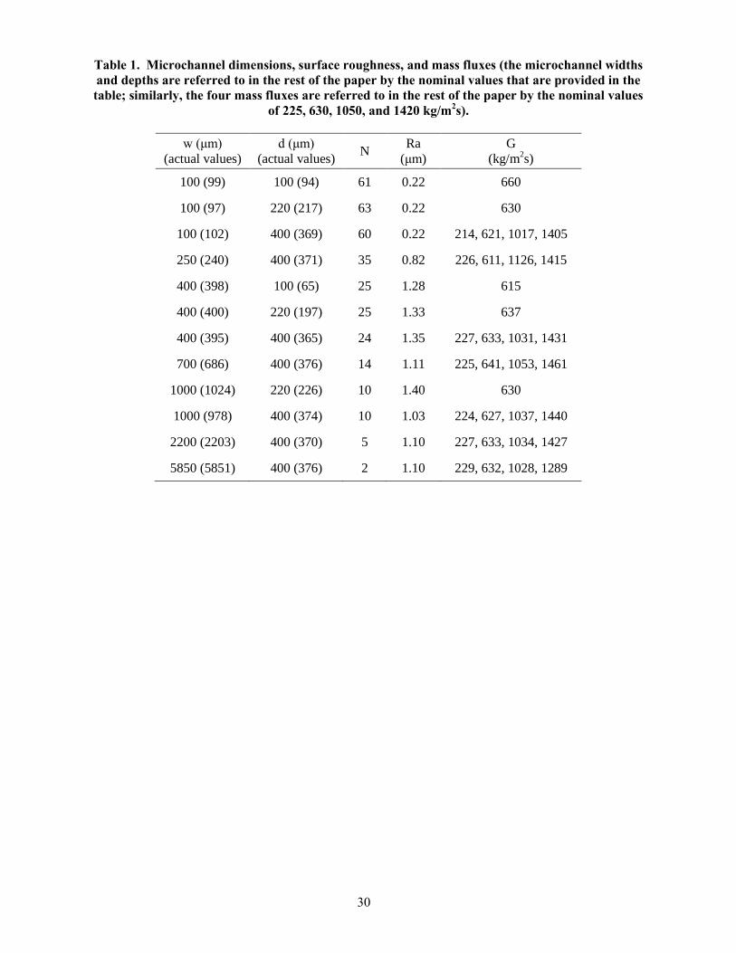
30

Table 1. Microchannel dimensions, surface roughness, and mass fluxes (the microchannel widths

and depths are referred to in the rest of the paper by the nominal values that are provided in the

table; similarly, the four mass fluxes are referred to in the rest of the paper by the nominal values

of 225, 630, 1050, and 1420 kg/m2s).

w (μm)

(actual values)

d (μm)

(actual values) N

Ra

(μm)

G

(kg/m2s)

100 (99) 100 (94) 61 0.22 660

100 (97) 220 (217) 63 0.22 630

100 (102) 400 (369) 60 0.22 214, 621, 1017, 1405

250 (240) 400 (371) 35 0.82 226, 611, 1126, 1415

400 (398) 100 (65) 25 1.28 615

400 (400) 220 (197) 25 1.33 637

400 (395) 400 (365) 24 1.35 227, 633, 1031, 1431

700 (686) 400 (376) 14 1.11 225, 641, 1053, 1461

1000 (1024) 220 (226) 10 1.40 630

1000 (978) 400 (374) 10 1.03 224, 627, 1037, 1440

2200 (2203) 400 (370) 5 1.10 227, 633, 1034, 1427

5850 (5851) 400 (376) 2 1.10 229, 632, 1028, 1289

31

Table 2. Studies in the literature from which heat transfer correlations are selected for comparison

against the current experimental data. Mean absolute error (MAE) and percentage of predictions

which fall within ±30% of the measurements are listed for each correlation.*

Correlation Fluid,

Geometry

MAE

(%)

Percentage of pred.

within ±30%

Cooper (pool boiling) [9] Water, refrigerants, organic fluids, cryogens 11.3 92.9

Gorenflo (pool boiling) [33] Several refrigerants, water and cryogenics 154 0

Chen [25] Water, Methanol, Pentane, Heptane,

Benzene,… 161.1 0

Shah [26] R11, R12, R22, R502,… 836 0

Bennett and Chen [34] Water, Methanol, Pentane, Heptane,

Benzene,… 186.3 1.6

Lazarek and Black [35] R113; Dh = 3.1 mm 149.6 0

Gungor and Winterton [27] Water, R11, R12, R113,...

Dh = 2.95-32.0 mm 484.1 0

Kandlikar [36] Water, R11, R12, R22, R113, Nitrogen,...

Dh = 4.6–32 mm 106.7 29.7

Liu and Winterton [37] Water and refrigerants; Dh = 2.95-32.0 mm 79.0 28.1

Steiner and Taborek [38] Water, refrigerants, cryogenics

Dh = 1 - 32 mm 148.1 0

Tran et al. [28] R12, R113; Dh = 2.4-2.92 mm 61.4 14.4

Yan and Lin [39] R134a; Dh = 2.0 mm 16248.6 2.6

Lee and Lee [40] R113; Dh = 0.78-3.6 mm 295.4 18.2

Warrier et al. [29] FC-84; Dh = 0.75 mm 68.1 27.2

Yu et al. [41] Water; Dh = 2.98 mm 4131.5 0

Haynes and Fletcher [42] R11, R123; Dh = 0.92-1.95 mm 126.6 0.6

Sumith et al. [43] Water; Dh = 1.45 mm 101.1 35.1

Balasubramanian and

Kandlikar [31]

Water, R113, R123, R141b,…

Dh = 0.19 - 2.92 mm 103.1 29.7

Thome et al. [10] R11, R12, R113, R123, R134a, R141b, CO2

Dh = 0.7-3.1 mm 43.4 39.3

Zhang et al. [30] Water, R11, R12, and R113

Dh = 0.78-6.0 mm 100.2 11.8

Lee and Mudawar [44] R134a, water; Dh = 0.35 mm 461.2 6.1

Yun et al. [45] R410A; Dh = 1.36, 1.44 mm 502.2 0

Liu and Garimella [32] Water; Dh = 0.38, 0.59 mm 83.7 31.9

Saitoh et al. [46] R134a; Dh = 0.5-11.0 mm 211.7 0

Lee and Garimella [47] Water; Dh = 0.16-0.57 mm 339.9 0

* Comparison is made to the experimental data in the 400 µm-deep microchannels only.

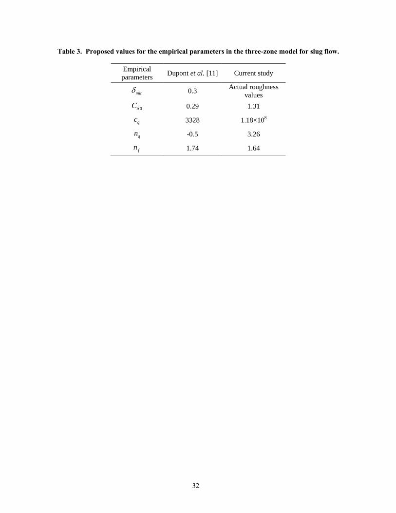
32

Table 3. Proposed values for the empirical parameters in the three-zone model for slug flow.

Empirical

parameters Dupont et al. [11] Current study

min 0.3 Actual roughness

values

0C 0.29 1.31

qc 3328 1.18×108

qn -0.5 3.26

fn 1.74 1.64

33

Expandable

reservoir

Heat

exchanger Pre-heater

Test section

High-speed

camera with

microscope

lens

Differential pressure

transducer

Pump

Figure 1. Photograph of the experimental facility [6].

34

(Bo)0.5

.Re

NZ

u

101

102

103

104

10-1

100

101

102

Confined Slug

Churn/Confined Annular

Bubbly

Churn/Wispy-Annular

Churn/Annular

0.5Bo Re 160

0.258

0.596.65 Bo RepchN

N

pch

Figure 2. Comprehensive flow regime map.

35

Pexp

(kPa)

P

pre

d(k

Pa

)

0 50 100 150 200 250 300 3500

50

100

150

200

250

300

350

-30%

+30%

MAE = 84.7%

23.2% of predictions within error of 30%

Pexp

(kPa)

P

pre

d(k

Pa

)

0 50 100 150 200 250 300 3500

50

100

150

200

250

300

350

-30%

+30%

12.8% of predictions within error of 30%

MAE = 186.0%

Pexp

(kPa)

P

pre

d(k

Pa

)

0 50 100 150 200 250 300 3500

50

100

150

200

250

300

350

-30%

+30%

MAE = 163.3%

7.4% of predictions within error of 30%

Pexp

(kPa)

P

pre

d(k

Pa

)

0 50 100 150 200 250 300 3500

50

100

150

200

250

300

350

-30%

+30%

MAE = 108.6%

21.1% of predictions within error of 30%

Pexp

(kPa)

P

pre

d(k

Pa

)

0 50 100 150 200 250 300 3500

50

100

150

200

250

300

350

-30%

+30%

MAE = 193.0%

4.4% of predictions within error of 30%

Pexp

(kPa)

P

pre

d(k

Pa

)

0 50 100 150 200 250 300 3500

50

100

150

200

250

300

350

-30%

+30%

MAE = 394.2%

4.7% of predictions within error of 30%

Lee & Mudawar [44]MAE = 394.2%

4.7% of predictions within ±30%

Lee & Garimella [47]MAE = 193.0%

4.4% of predictions within ±30%

Lee & Lee [40]MAE = 108.6%

21.1% of predictions within ±30%

Qu & Mudawar [17]MAE = 163.3%

7.4% of predictions within ±30%

Lockhart & Martinelli [53]MAE = 186.0%

12.8% of predictions within ±30%

Mishima & Hibiki [54]MAE = 84.7%

23.2% of predictions within ±30%

Figure 3. Comparison of the experimentally measured pressure drop across microchannels [4, 5]

with predictions from empirical correlations in the literature.

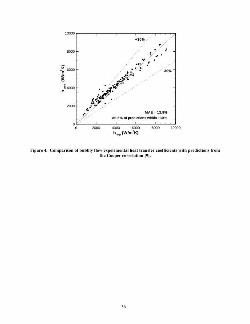
36

hexp

(W/m2K)

hp

red

(W/m

2K

)

0 2000 4000 6000 8000 100000

2000

4000

6000

8000

10000

+30%

-30%

MAE = 13.9%

86.5% of predictions within 30%

Figure 4. Comparison of bubbly flow experimental heat transfer coefficients with predictions from

the Cooper correlation [9].

37

(a)

δ

δ

Δz Δz

Liquid film

CV

Vapor core

CV

y

(b)

Figure 5. (a) Schematic representation of annular flow in microchannels, and (b) simplified flow

diagram with vapor core and liquid film control volumes.

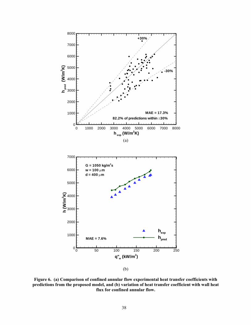
38

hexp

(W/m2K)

hp

red

(W/m

2K

)

0 1000 2000 3000 4000 5000 6000 7000 80000

1000

2000

3000

4000

5000

6000

7000

8000

+30%

-30%

MAE = 17.3%

82.2% of predictions within 30%

(a)

q"w

(kW/m2)

h(W

/m2K

)

0 50 100 150 200 2500

1000

2000

3000

4000

5000

6000

7000

hexp

hpred

G = 1050 kg/m2s

w = 100 m

d = 400 m

MAE = 7.6%

(b)

Figure 6. (a) Comparison of confined annular flow experimental heat transfer coefficients with

predictions from the proposed model, and (b) variation of heat transfer coefficient with wall heat

flux for confined annular flow.

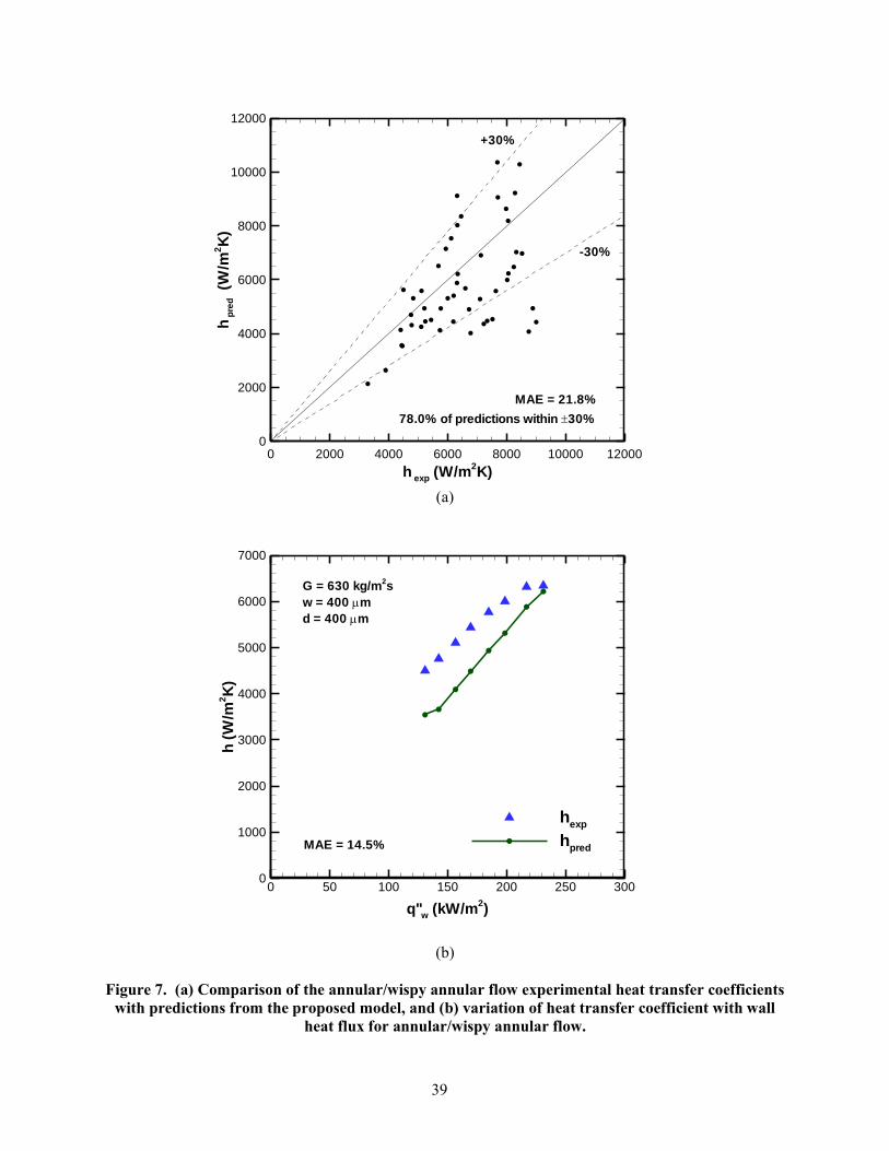
39

hexp

(W/m2K)

hp

red

(W/m

2K

)

0 2000 4000 6000 8000 10000 120000

2000

4000

6000

8000

10000

12000

+30%

-30%

MAE = 21.8%

78.0% of predictions within 30%

(a)

q"w

(kW/m2)

h(W

/m2K

)

0 50 100 150 200 250 3000

1000

2000

3000

4000

5000

6000

7000

hexp

hpred

G = 630 kg/m2s

w = 400 m

d = 400 m

MAE = 14.5%

(b)

Figure 7. (a) Comparison of the annular/wispy annular flow experimental heat transfer coefficients

with predictions from the proposed model, and (b) variation of heat transfer coefficient with wall

heat flux for annular/wispy annular flow.

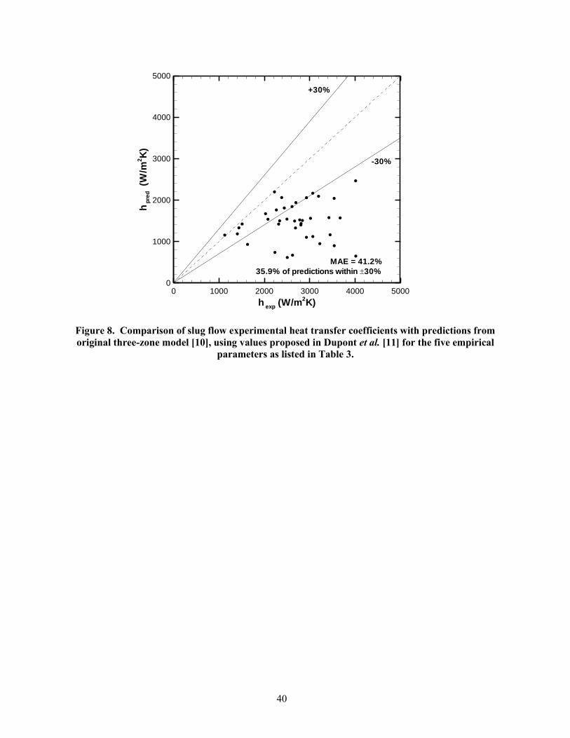
40

hexp

(W/m2K)

hp

red

(W/m

2K

)

0 1000 2000 3000 4000 50000

1000

2000

3000

4000

5000

+30%

-30%

MAE = 41.2%

35.9% of predictions within 30%

Figure 8. Comparison of slug flow experimental heat transfer coefficients with predictions from

original three-zone model [10], using values proposed in Dupont et al. [11] for the five empirical

parameters as listed in Table 3.

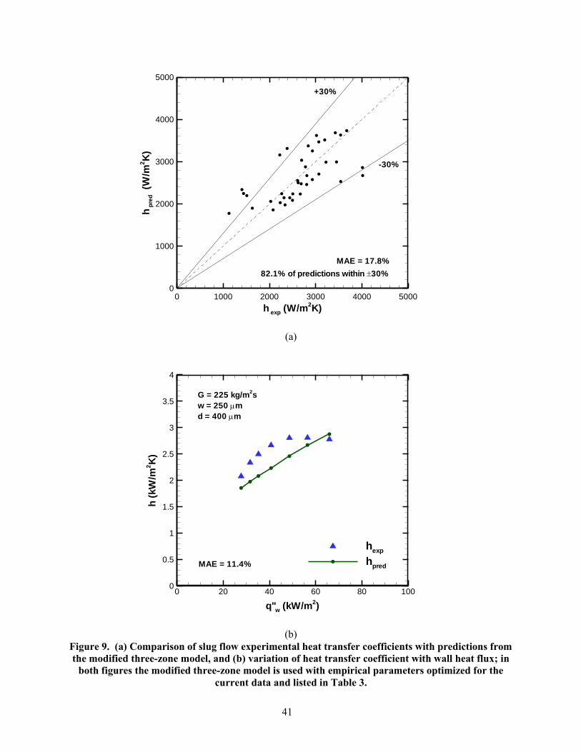
41

hexp

(W/m2K)

hp

red

(W/m

2K

)

0 1000 2000 3000 4000 50000

1000

2000

3000

4000

5000

+30%

-30%

MAE = 17.8%

82.1% of predictions within 30%

(a)

q"w

(kW/m2)

h(k

W/m

2K

)

0 20 40 60 80 1000

0.5

1

1.5

2

2.5

3

3.5

4

hexp

hpred

G = 225 kg/m2s

w = 250 m

d = 400 m

MAE = 11.4%

(b)

Figure 9. (a) Comparison of slug flow experimental heat transfer coefficients with predictions from

the modified three-zone model, and (b) variation of heat transfer coefficient with wall heat flux; in

both figures the modified three-zone model is used with empirical parameters optimized for the

current data and listed in Table 3.

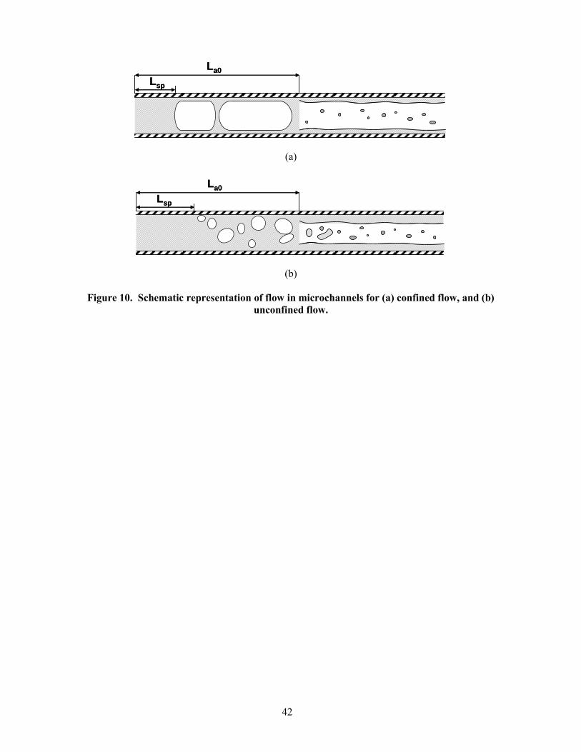
42

Lsp

La0

Lsp

La0

(a)

Lsp

La0

Lsp

La0

(b)

Figure 10. Schematic representation of flow in microchannels for (a) confined flow, and (b)

unconfined flow.

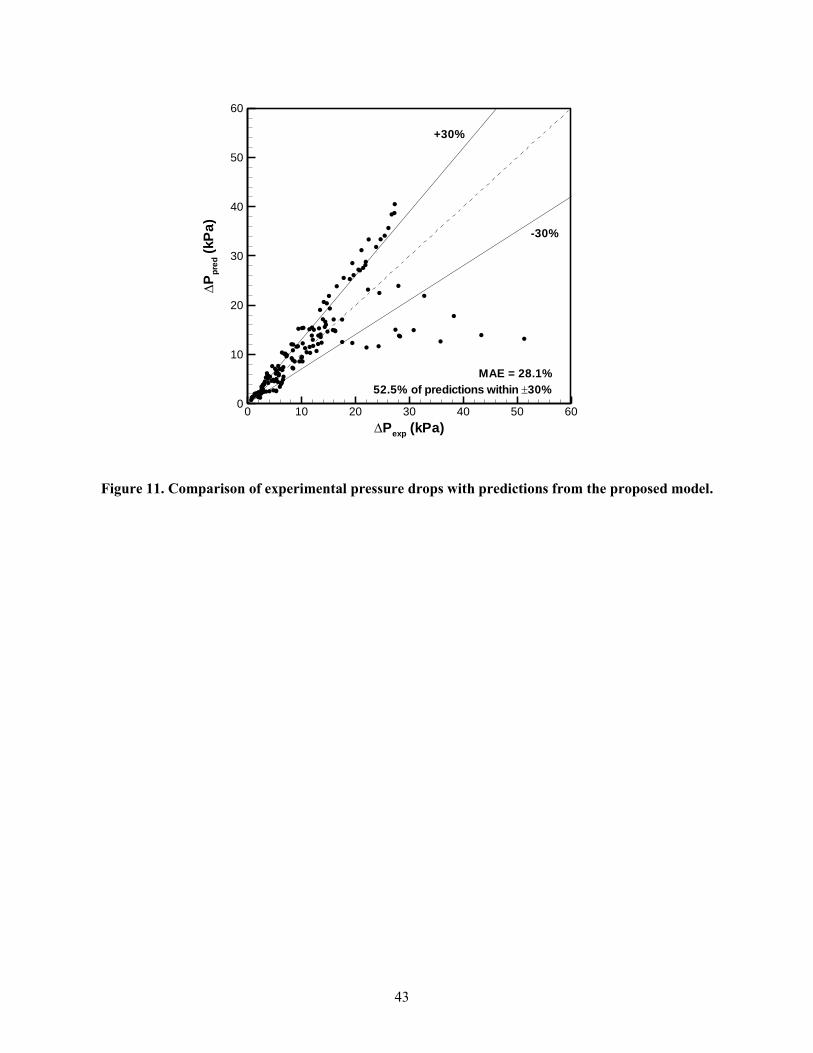
43

Pexp

(kPa)

P

pre

d(k

Pa

)

0 10 20 30 40 50 600

10

20

30

40

50

60

-30%

+30%

52.5% of predictions within 30%

MAE = 28.1%

Figure 11. Comparison of experimental pressure drops with predictions from the proposed model.