fluid dynamics - uni-
TRANSCRIPT

Fluid Dynamics for Engineers
Dominique Thevenin (TEX version) & Gabor Janiga (WWW version)
July 10, 2014

Copyright c©2009-2014 D. Thevenin & G. Janiga. Permission is granted to copy, distribute and/ormodify this document under the terms of the GNU Free Documentation License, Version 1.3 or anylater version published by the Free Software Foundation; with no Invariant Sections, no Front-CoverTexts, and no Back-Cover Texts. A copy of the license is included in the Appendix entitled “GNU FreeDocumentation License”.

Contents
Preface 9
List of symbols 11
1 Introduction 17
1.1 Practical importance of fluid dynamics . . . . . . . . . . . . . . . . . . . . . . . . . . . . 17
1.2 What is a fluid? . . . . . . . . . . . . . . . . . . . . . . . . . . . . . . . . . . . . . . . . . 17
1.3 Continuum assumption . . . . . . . . . . . . . . . . . . . . . . . . . . . . . . . . . . . . . 18
1.4 Important flow variables and variable-based classification . . . . . . . . . . . . . . . . . . 20
2 Basic concepts 23
2.1 Mathematical operators . . . . . . . . . . . . . . . . . . . . . . . . . . . . . . . . . . . . 23
2.1.1 Gradient . . . . . . . . . . . . . . . . . . . . . . . . . . . . . . . . . . . . . . . . . 23
2.1.2 Divergence . . . . . . . . . . . . . . . . . . . . . . . . . . . . . . . . . . . . . . . . 24
2.1.3 Laplacian . . . . . . . . . . . . . . . . . . . . . . . . . . . . . . . . . . . . . . . . 25
2.1.4 Rotor or Curl . . . . . . . . . . . . . . . . . . . . . . . . . . . . . . . . . . . . . . 26
2.2 Time derivatives . . . . . . . . . . . . . . . . . . . . . . . . . . . . . . . . . . . . . . . . 26
2.3 Characteristic flow structures . . . . . . . . . . . . . . . . . . . . . . . . . . . . . . . . . 28
2.4 Control volume . . . . . . . . . . . . . . . . . . . . . . . . . . . . . . . . . . . . . . . . . 31
2.5 Transport theorem . . . . . . . . . . . . . . . . . . . . . . . . . . . . . . . . . . . . . . . 33
3 Mass conservation 35
3.1 Introduction . . . . . . . . . . . . . . . . . . . . . . . . . . . . . . . . . . . . . . . . . . 35
3.2 Point of view of physics . . . . . . . . . . . . . . . . . . . . . . . . . . . . . . . . . . . . . 35
3.3 Point of view of mathematics . . . . . . . . . . . . . . . . . . . . . . . . . . . . . . . . . 35
3.4 Integral formulation of mass conservation . . . . . . . . . . . . . . . . . . . . . . . . . . . 36
3.5 Local formulation of mass conservation . . . . . . . . . . . . . . . . . . . . . . . . . . . . 36
3.5.1 Local formulation of mass conservation in cylindrical coordinates . . . . . . . . . . 37
3.6 Local mass conservation for an incompressible flow . . . . . . . . . . . . . . . . . . . . . 37
4 Euler equation: conservation of momentum in a non-viscous flow 39
4.1 Introduction . . . . . . . . . . . . . . . . . . . . . . . . . . . . . . . . . . . . . . . . . . 39
4.2 Point of view of mathematics . . . . . . . . . . . . . . . . . . . . . . . . . . . . . . . . . 39
4.3 Point of view of physics . . . . . . . . . . . . . . . . . . . . . . . . . . . . . . . . . . . . . 40
4.4 Integral formulation of momentum conservation . . . . . . . . . . . . . . . . . . . . . . . 41
4.5 Local formulation of momentum conservation . . . . . . . . . . . . . . . . . . . . . . . . 42
4.6 Local momentum conservation for an incompressible flow . . . . . . . . . . . . . . . . . . 43
4.7 Integral formulation of angular momentum conservation . . . . . . . . . . . . . . . . . . . 43
1

2
5 Hydrostatics and Aerostatics 455.1 Introduction . . . . . . . . . . . . . . . . . . . . . . . . . . . . . . . . . . . . . . . . . . 455.2 Fundamental equation of hydro- and aerostatics . . . . . . . . . . . . . . . . . . . . . . . 455.3 Pressure variation within an incompressible, static fluid . . . . . . . . . . . . . . . . . . . 475.4 Force exerted by an incompressible, static fluid, on a fully immersed body . . . . . . . . . 495.5 Force exerted on a partially immersed body . . . . . . . . . . . . . . . . . . . . . . . . . 545.6 Stability of a partially immersed body . . . . . . . . . . . . . . . . . . . . . . . . . . . . 555.7 Aerostatics . . . . . . . . . . . . . . . . . . . . . . . . . . . . . . . . . . . . . . . . . . . . 58
5.7.1 Pressure variation in an isothermal, ideal gas . . . . . . . . . . . . . . . . . . . . . 595.7.2 Principle of Archimedes in a gas . . . . . . . . . . . . . . . . . . . . . . . . . . . . 60
6 Bernoulli equations 616.1 Introduction . . . . . . . . . . . . . . . . . . . . . . . . . . . . . . . . . . . . . . . . . . 616.2 Bernoulli equation for an irrotational flow . . . . . . . . . . . . . . . . . . . . . . . . . . 616.3 Link with hydrostatics . . . . . . . . . . . . . . . . . . . . . . . . . . . . . . . . . . . . . 636.4 Bernoulli equation (for a rotational flow) . . . . . . . . . . . . . . . . . . . . . . . . . . . 636.5 The Bernoulli triangle . . . . . . . . . . . . . . . . . . . . . . . . . . . . . . . . . . . . . 646.6 Simplification of the Bernoulli equation for a gas flow . . . . . . . . . . . . . . . . . . . . 656.7 Dynamic pressure . . . . . . . . . . . . . . . . . . . . . . . . . . . . . . . . . . . . . . . . 666.8 Averaged Bernoulli equation . . . . . . . . . . . . . . . . . . . . . . . . . . . . . . . . . . 666.9 Hydraulic height . . . . . . . . . . . . . . . . . . . . . . . . . . . . . . . . . . . . . . . . 686.10 Generalized Bernoulli equation with losses and energy exchange . . . . . . . . . . . . . . 69
6.10.1 Computing the exchanged specific work w . . . . . . . . . . . . . . . . . . . . . . 716.10.2 Computing the friction loss ∆ef . . . . . . . . . . . . . . . . . . . . . . . . . . . . 716.10.3 Numerical equations used to estimate the friction factor f . . . . . . . . . . . . . 736.10.4 Computing a localized loss ∆el . . . . . . . . . . . . . . . . . . . . . . . . . . . . 74
7 Force and torque exerted by a flow 777.1 Introduction . . . . . . . . . . . . . . . . . . . . . . . . . . . . . . . . . . . . . . . . . . 777.2 Force exerted by a flow on its surroundings . . . . . . . . . . . . . . . . . . . . . . . . . . 787.3 Force exerted by a flow on a pipe wall surrounded by a fluid at constant pressure . . . . . 807.4 Torque exerted by a flow on its surroundings . . . . . . . . . . . . . . . . . . . . . . . . . 827.5 Torque exerted by a flow on a pipe wall surrounded by a fluid at constant pressure . . . . 86
8 Movement of a material control volume 898.1 Introduction . . . . . . . . . . . . . . . . . . . . . . . . . . . . . . . . . . . . . . . . . . 898.2 Movement of a material control volume . . . . . . . . . . . . . . . . . . . . . . . . . . . . 898.3 Deformation tensor d . . . . . . . . . . . . . . . . . . . . . . . . . . . . . . . . . . . . . . 938.4 Rotation tensor Ω . . . . . . . . . . . . . . . . . . . . . . . . . . . . . . . . . . . . . . . . 94
9 Navier-Stokes equation: conservation of momentum in a viscous flow 979.1 Introduction . . . . . . . . . . . . . . . . . . . . . . . . . . . . . . . . . . . . . . . . . . 979.2 Point of view of mathematics . . . . . . . . . . . . . . . . . . . . . . . . . . . . . . . . . 979.3 Point of view of physics . . . . . . . . . . . . . . . . . . . . . . . . . . . . . . . . . . . . . 98
9.3.1 Pressure component Tp of the stress tensor σ . . . . . . . . . . . . . . . . . . . . . 989.3.2 Friction component τ of the stress tensor σ . . . . . . . . . . . . . . . . . . . . . . 999.3.3 Full stress tensor σ . . . . . . . . . . . . . . . . . . . . . . . . . . . . . . . . . . . 100
9.4 Integral formulation of momentum conservation . . . . . . . . . . . . . . . . . . . . . . . 1009.5 Local formulation of momentum conservation . . . . . . . . . . . . . . . . . . . . . . . . 101

3
9.6 Local momentum conservation for an incompressible flow . . . . . . . . . . . . . . . . . . 1029.7 Local formulation of momentum conservation for a non-Newtonian fluid . . . . . . . . . . 1039.8 Local formulation of momentum conservation for a Newtonian fluid . . . . . . . . . . . . 1039.9 Local formulation of momentum conservation (incompressible flow, Newtonian fluid) . . . 103
9.9.1 Local formulation of momentum conservation in cylindrical coordinates . . . . . . 104
10 Dimensional analysis and similarity conditions 10510.1 Introduction . . . . . . . . . . . . . . . . . . . . . . . . . . . . . . . . . . . . . . . . . . 10510.2 Non-dimensional conservation equations . . . . . . . . . . . . . . . . . . . . . . . . . . . 105
10.2.1 Non-dimensional mass conservation for an incompressible flow . . . . . . . . . . . 10710.2.2 Non-dimensional momentum conservation (incompressible flow, Newtonian fluid) . 107
10.3 Non-dimensional parameters of Fluid Dynamics . . . . . . . . . . . . . . . . . . . . . . . 10810.3.1 Strouhal number St . . . . . . . . . . . . . . . . . . . . . . . . . . . . . . . . . . . 10810.3.2 Froude number Fr . . . . . . . . . . . . . . . . . . . . . . . . . . . . . . . . . . . . 10910.3.3 Euler number Eu . . . . . . . . . . . . . . . . . . . . . . . . . . . . . . . . . . . . 11010.3.4 Reynolds number Re . . . . . . . . . . . . . . . . . . . . . . . . . . . . . . . . . . 11010.3.5 Further non-dimensional parameters . . . . . . . . . . . . . . . . . . . . . . . . . 11110.3.6 Choosing the reference quantities . . . . . . . . . . . . . . . . . . . . . . . . . . . 11210.3.7 Summary: non-dimensional conservation equations . . . . . . . . . . . . . . . . . 112
10.4 A faster solution: the Π-theorem . . . . . . . . . . . . . . . . . . . . . . . . . . . . . . . 11310.5 Relevant dimensional variables . . . . . . . . . . . . . . . . . . . . . . . . . . . . . . . . . 11410.6 Similarity conditions in Fluid Dynamics . . . . . . . . . . . . . . . . . . . . . . . . . . . 115
11 One-dimensional isentropic compressible flows 11711.1 Introduction and hypotheses . . . . . . . . . . . . . . . . . . . . . . . . . . . . . . . . . . 11711.2 Generic relations, also valid for a real gas . . . . . . . . . . . . . . . . . . . . . . . . . . . 118
11.2.1 Conservation equations . . . . . . . . . . . . . . . . . . . . . . . . . . . . . . . . . 11811.2.2 What is a compressible gas flow? . . . . . . . . . . . . . . . . . . . . . . . . . . . 12211.2.3 Influence of a modification of the cross-section A . . . . . . . . . . . . . . . . . . . 12311.2.4 Critical conditions . . . . . . . . . . . . . . . . . . . . . . . . . . . . . . . . . . . 12411.2.5 Laval nozzle . . . . . . . . . . . . . . . . . . . . . . . . . . . . . . . . . . . . . . . 126
11.3 Specific relations for a compressible flow of a perfect gas . . . . . . . . . . . . . . . . . . 12811.3.1 What is a perfect gas? . . . . . . . . . . . . . . . . . . . . . . . . . . . . . . . . . 12811.3.2 Isentropic relations for a perfect gas . . . . . . . . . . . . . . . . . . . . . . . . . . 12911.3.3 Speed of sound for a perfect gas . . . . . . . . . . . . . . . . . . . . . . . . . . . . 13011.3.4 Analytical solution for a compressible flow of a perfect gas . . . . . . . . . . . . . 13011.3.5 Critical conditions . . . . . . . . . . . . . . . . . . . . . . . . . . . . . . . . . . . 13311.3.6 Solution procedure and remaining difficulties . . . . . . . . . . . . . . . . . . . . . 13411.3.7 Minimal stagnation pressure for a properly working Laval-nozzle . . . . . . . . . . 13511.3.8 Tables for compressible flows . . . . . . . . . . . . . . . . . . . . . . . . . . . . . . 13511.3.9 Solution using the critical Mach number M∗ . . . . . . . . . . . . . . . . . . . . . 13511.3.10Discharge velocity vd . . . . . . . . . . . . . . . . . . . . . . . . . . . . . . . . . . 136
11.4 Conclusions . . . . . . . . . . . . . . . . . . . . . . . . . . . . . . . . . . . . . . . . . . . 136
12 Compressible flows with friction and heat exchange 13912.1 Introduction and hypotheses . . . . . . . . . . . . . . . . . . . . . . . . . . . . . . . . . . 13912.2 Generic relations, also valid for a real gas . . . . . . . . . . . . . . . . . . . . . . . . . . . 140
12.2.1 Conservation equations . . . . . . . . . . . . . . . . . . . . . . . . . . . . . . . . . 14012.2.2 Generalized equation of Hugoniot . . . . . . . . . . . . . . . . . . . . . . . . . . . 143

4
12.2.3 Pressure variation for a constant flow cross-section . . . . . . . . . . . . . . . . . . 145
12.3 Influence of heat exchange in a perfect gas . . . . . . . . . . . . . . . . . . . . . . . . . . 147
12.3.1 Mass conservation . . . . . . . . . . . . . . . . . . . . . . . . . . . . . . . . . . . . 147
12.3.2 Conservation of momentum . . . . . . . . . . . . . . . . . . . . . . . . . . . . . . 148
12.3.3 Energy conservation . . . . . . . . . . . . . . . . . . . . . . . . . . . . . . . . . . 148
12.3.4 Solution procedure . . . . . . . . . . . . . . . . . . . . . . . . . . . . . . . . . . . 149
12.3.5 Flow modifications . . . . . . . . . . . . . . . . . . . . . . . . . . . . . . . . . . . 151
12.3.6 Thermal choking . . . . . . . . . . . . . . . . . . . . . . . . . . . . . . . . . . . . 153
12.4 Influence of friction . . . . . . . . . . . . . . . . . . . . . . . . . . . . . . . . . . . . . . . 153
12.4.1 Mass conservation . . . . . . . . . . . . . . . . . . . . . . . . . . . . . . . . . . . . 154
12.4.2 Conservation of momentum . . . . . . . . . . . . . . . . . . . . . . . . . . . . . . 154
12.4.3 Energy conservation . . . . . . . . . . . . . . . . . . . . . . . . . . . . . . . . . . 155
12.4.4 Qualitative analysis . . . . . . . . . . . . . . . . . . . . . . . . . . . . . . . . . . . 155
12.4.5 Quantitative solution procedure . . . . . . . . . . . . . . . . . . . . . . . . . . . . 155
12.4.6 Flow modifications . . . . . . . . . . . . . . . . . . . . . . . . . . . . . . . . . . . 158
12.5 Conclusions . . . . . . . . . . . . . . . . . . . . . . . . . . . . . . . . . . . . . . . . . . . 158
13 Shock waves 161
13.1 Introduction . . . . . . . . . . . . . . . . . . . . . . . . . . . . . . . . . . . . . . . . . . . 161
13.2 Normal shock wave . . . . . . . . . . . . . . . . . . . . . . . . . . . . . . . . . . . . . . . 162
13.2.1 Considered configuration and hypotheses . . . . . . . . . . . . . . . . . . . . . . . 162
13.2.2 Conservation equations for a real gas . . . . . . . . . . . . . . . . . . . . . . . . . 162
13.2.3 Conservation equations for a perfect gas . . . . . . . . . . . . . . . . . . . . . . . 163
13.2.4 Jump relations involving M1 and M2 . . . . . . . . . . . . . . . . . . . . . . . . . 164
13.2.5 Relation between the Mach numbers upstream and downstream of the normal shock165
13.2.6 Jump relations involving only the upstream Mach number M1 . . . . . . . . . . . 166
13.2.7 Necessary condition on M1 for the existence of a shock . . . . . . . . . . . . . . . 171
13.2.8 Shock relation of Prandtl . . . . . . . . . . . . . . . . . . . . . . . . . . . . . . . . 172
13.2.9 Summary: evolution of all quantities through a normal shock . . . . . . . . . . . . 173
13.2.10Normal shock tables . . . . . . . . . . . . . . . . . . . . . . . . . . . . . . . . . . 173
13.2.11Solution and graphical representation using the critical Mach number . . . . . . . 174
13.2.12Relation of Rankine-Hugoniot . . . . . . . . . . . . . . . . . . . . . . . . . . . . . 174
13.2.13Rayleigh line . . . . . . . . . . . . . . . . . . . . . . . . . . . . . . . . . . . . . . 175
13.2.14Propagating shock waves . . . . . . . . . . . . . . . . . . . . . . . . . . . . . . . . 176
13.3 Why shock waves? . . . . . . . . . . . . . . . . . . . . . . . . . . . . . . . . . . . . . . . 179
13.4 Oblique shock wave . . . . . . . . . . . . . . . . . . . . . . . . . . . . . . . . . . . . . . . 180
13.4.1 Conservation equations for a real gas . . . . . . . . . . . . . . . . . . . . . . . . . 182
13.4.2 Conservation equations for a perfect gas . . . . . . . . . . . . . . . . . . . . . . . 184
13.4.3 Jump relations involving the upstream Mach number M1 . . . . . . . . . . . . . . 186
13.4.4 Summary: evolution of all quantities through an oblique shock . . . . . . . . . . . 187
13.4.5 Using the shock tables for an oblique shock . . . . . . . . . . . . . . . . . . . . . . 187
13.4.6 Determining the shock angle ε . . . . . . . . . . . . . . . . . . . . . . . . . . . . . 188
13.4.7 Mach angle and Mach wave . . . . . . . . . . . . . . . . . . . . . . . . . . . . . . 191
13.5 Polar curve and Busemann diagram . . . . . . . . . . . . . . . . . . . . . . . . . . . . . . 191
13.6 Boundary conditions and shock reflections . . . . . . . . . . . . . . . . . . . . . . . . . . 193
13.7 Conclusions . . . . . . . . . . . . . . . . . . . . . . . . . . . . . . . . . . . . . . . . . . . 194

5
14 Introduction to turbulence 19714.1 Turbulence: complexity and importance . . . . . . . . . . . . . . . . . . . . . . . . . . . 19714.2 A first taste of turbulence: the experiment of Reynolds . . . . . . . . . . . . . . . . . . . 19814.3 Qualitative properties of turbulent flows . . . . . . . . . . . . . . . . . . . . . . . . . . . 199
A Basic concepts and keywords of fluid dynamics 201A.1 Archimedes number . . . . . . . . . . . . . . . . . . . . . . . . . . . . . . . . . . . . . . . 201A.2 Cavitation . . . . . . . . . . . . . . . . . . . . . . . . . . . . . . . . . . . . . . . . . . . . 201A.3 Compressible flow . . . . . . . . . . . . . . . . . . . . . . . . . . . . . . . . . . . . . . . . 202A.4 Compressible fluid . . . . . . . . . . . . . . . . . . . . . . . . . . . . . . . . . . . . . . . 202A.5 Conservative force . . . . . . . . . . . . . . . . . . . . . . . . . . . . . . . . . . . . . . . . 202A.6 Contact force vs. non-contact force . . . . . . . . . . . . . . . . . . . . . . . . . . . . . . 202A.7 Hydraulic diameter . . . . . . . . . . . . . . . . . . . . . . . . . . . . . . . . . . . . . . . 203A.8 Incompressible flow . . . . . . . . . . . . . . . . . . . . . . . . . . . . . . . . . . . . . . . 203A.9 Incompressible fluid . . . . . . . . . . . . . . . . . . . . . . . . . . . . . . . . . . . . . . . 204A.10 Internal flow . . . . . . . . . . . . . . . . . . . . . . . . . . . . . . . . . . . . . . . . . . . 206A.11 Irrotational flow . . . . . . . . . . . . . . . . . . . . . . . . . . . . . . . . . . . . . . . . . 206A.12 Laminar flow . . . . . . . . . . . . . . . . . . . . . . . . . . . . . . . . . . . . . . . . . . 206A.13 Mach number . . . . . . . . . . . . . . . . . . . . . . . . . . . . . . . . . . . . . . . . . . 206A.14 Multiphase flow . . . . . . . . . . . . . . . . . . . . . . . . . . . . . . . . . . . . . . . . . 206A.15 Newtonian fluid . . . . . . . . . . . . . . . . . . . . . . . . . . . . . . . . . . . . . . . . . 206A.16 Non-Newtonian fluid . . . . . . . . . . . . . . . . . . . . . . . . . . . . . . . . . . . . . . 207A.17 Non-viscous flow . . . . . . . . . . . . . . . . . . . . . . . . . . . . . . . . . . . . . . . . 207A.18 One-dimensional flow . . . . . . . . . . . . . . . . . . . . . . . . . . . . . . . . . . . . . . 208A.19 Open channel flow . . . . . . . . . . . . . . . . . . . . . . . . . . . . . . . . . . . . . . . 208A.20 Potential flow . . . . . . . . . . . . . . . . . . . . . . . . . . . . . . . . . . . . . . . . . . 208A.21 Quasi-steady flow . . . . . . . . . . . . . . . . . . . . . . . . . . . . . . . . . . . . . . . . 208A.22 Speed of sound . . . . . . . . . . . . . . . . . . . . . . . . . . . . . . . . . . . . . . . . . 208A.23 Standard coordinate system . . . . . . . . . . . . . . . . . . . . . . . . . . . . . . . . . . 209A.24 Steady flow . . . . . . . . . . . . . . . . . . . . . . . . . . . . . . . . . . . . . . . . . . . 209A.25 Stress in a fluid . . . . . . . . . . . . . . . . . . . . . . . . . . . . . . . . . . . . . . . . . 210A.26 Turbulent flow . . . . . . . . . . . . . . . . . . . . . . . . . . . . . . . . . . . . . . . . . . 211A.27 Unsteady flow . . . . . . . . . . . . . . . . . . . . . . . . . . . . . . . . . . . . . . . . . . 211A.28 vena contracta . . . . . . . . . . . . . . . . . . . . . . . . . . . . . . . . . . . . . . . . . . 211A.29 Viscosity . . . . . . . . . . . . . . . . . . . . . . . . . . . . . . . . . . . . . . . . . . . . . 212
B Basic thermodynamic concepts needed for fluid dynamics 213B.1 Adiabatic process . . . . . . . . . . . . . . . . . . . . . . . . . . . . . . . . . . . . . . . . 213B.2 Barotropic state . . . . . . . . . . . . . . . . . . . . . . . . . . . . . . . . . . . . . . . . . 213B.3 Enthalpy . . . . . . . . . . . . . . . . . . . . . . . . . . . . . . . . . . . . . . . . . . . . . 213B.4 Entropy . . . . . . . . . . . . . . . . . . . . . . . . . . . . . . . . . . . . . . . . . . . . . 214B.5 Gas constant . . . . . . . . . . . . . . . . . . . . . . . . . . . . . . . . . . . . . . . . . . 214B.6 Heat capacity . . . . . . . . . . . . . . . . . . . . . . . . . . . . . . . . . . . . . . . . . . 214B.7 Heat capacity ratio . . . . . . . . . . . . . . . . . . . . . . . . . . . . . . . . . . . . . . . 215B.8 Ideal gas . . . . . . . . . . . . . . . . . . . . . . . . . . . . . . . . . . . . . . . . . . . . . 215B.9 Isentropic transformation . . . . . . . . . . . . . . . . . . . . . . . . . . . . . . . . . . . . 215B.10 Isobaric transformation . . . . . . . . . . . . . . . . . . . . . . . . . . . . . . . . . . . . . 215B.11 Isochoric transformation . . . . . . . . . . . . . . . . . . . . . . . . . . . . . . . . . . . . 216B.12 Isothermal transformation . . . . . . . . . . . . . . . . . . . . . . . . . . . . . . . . . . . 216
6
B.13 Perfect gas . . . . . . . . . . . . . . . . . . . . . . . . . . . . . . . . . . . . . . . . . . . . 216B.14 Polytropic process . . . . . . . . . . . . . . . . . . . . . . . . . . . . . . . . . . . . . . . . 216B.15 Prandtl number . . . . . . . . . . . . . . . . . . . . . . . . . . . . . . . . . . . . . . . . . 217B.16 Real gas . . . . . . . . . . . . . . . . . . . . . . . . . . . . . . . . . . . . . . . . . . . . . 217B.17 Reversible process . . . . . . . . . . . . . . . . . . . . . . . . . . . . . . . . . . . . . . . . 217B.18 Specific quantity . . . . . . . . . . . . . . . . . . . . . . . . . . . . . . . . . . . . . . . . 217B.19 Standard thermodynamic conditions . . . . . . . . . . . . . . . . . . . . . . . . . . . . . 218B.20 Thermal conductivity . . . . . . . . . . . . . . . . . . . . . . . . . . . . . . . . . . . . . . 218
C Basic mathematical concepts needed for fluid dynamics 219C.1 Angular relations in a right triangle . . . . . . . . . . . . . . . . . . . . . . . . . . . . . . 219C.2 Conic curves . . . . . . . . . . . . . . . . . . . . . . . . . . . . . . . . . . . . . . . . . . . 220C.3 Divergence theorem . . . . . . . . . . . . . . . . . . . . . . . . . . . . . . . . . . . . . . . 220C.4 Summation convention of Einstein . . . . . . . . . . . . . . . . . . . . . . . . . . . . . . . 220C.5 Logarithmic differential . . . . . . . . . . . . . . . . . . . . . . . . . . . . . . . . . . . . . 221C.6 Partial derivative . . . . . . . . . . . . . . . . . . . . . . . . . . . . . . . . . . . . . . . . 221C.7 Scalar product . . . . . . . . . . . . . . . . . . . . . . . . . . . . . . . . . . . . . . . . . . 221C.8 Surfaces and volumes . . . . . . . . . . . . . . . . . . . . . . . . . . . . . . . . . . . . . . 221
C.8.1 Circle or disk . . . . . . . . . . . . . . . . . . . . . . . . . . . . . . . . . . . . . . 221C.8.2 Sphere . . . . . . . . . . . . . . . . . . . . . . . . . . . . . . . . . . . . . . . . . . 221C.8.3 Cylinder . . . . . . . . . . . . . . . . . . . . . . . . . . . . . . . . . . . . . . . . . 222C.8.4 Cone . . . . . . . . . . . . . . . . . . . . . . . . . . . . . . . . . . . . . . . . . . . 222
C.9 Vectors . . . . . . . . . . . . . . . . . . . . . . . . . . . . . . . . . . . . . . . . . . . . . . 222C.10 Vector product . . . . . . . . . . . . . . . . . . . . . . . . . . . . . . . . . . . . . . . . . 222C.11 Taylor expansion . . . . . . . . . . . . . . . . . . . . . . . . . . . . . . . . . . . . . . . . 222C.12 Tensors . . . . . . . . . . . . . . . . . . . . . . . . . . . . . . . . . . . . . . . . . . . . . 223
D Biography of selected important scientists 225D.1 Archimedes . . . . . . . . . . . . . . . . . . . . . . . . . . . . . . . . . . . . . . . . . . . 225D.2 Amedeo Avogadro . . . . . . . . . . . . . . . . . . . . . . . . . . . . . . . . . . . . . . . 225D.3 Daniel Bernoulli . . . . . . . . . . . . . . . . . . . . . . . . . . . . . . . . . . . . . . . . . 225D.4 Blasius . . . . . . . . . . . . . . . . . . . . . . . . . . . . . . . . . . . . . . . . . . . . . . 225D.5 Ludwig Boltzmann . . . . . . . . . . . . . . . . . . . . . . . . . . . . . . . . . . . . . . . 225D.6 Edgar Buckingham . . . . . . . . . . . . . . . . . . . . . . . . . . . . . . . . . . . . . . . 225D.7 Adolf Busemann . . . . . . . . . . . . . . . . . . . . . . . . . . . . . . . . . . . . . . . . 225D.8 Henry Darcy . . . . . . . . . . . . . . . . . . . . . . . . . . . . . . . . . . . . . . . . . . . 226D.9 Leonard Euler . . . . . . . . . . . . . . . . . . . . . . . . . . . . . . . . . . . . . . . . . . 226D.10 Richard Feynman . . . . . . . . . . . . . . . . . . . . . . . . . . . . . . . . . . . . . . . . 226D.11 William Froude . . . . . . . . . . . . . . . . . . . . . . . . . . . . . . . . . . . . . . . . . 226D.12 Otto von Guericke . . . . . . . . . . . . . . . . . . . . . . . . . . . . . . . . . . . . . . . 226D.13 Galileo Galilei . . . . . . . . . . . . . . . . . . . . . . . . . . . . . . . . . . . . . . . . . . 226D.14 Carl Friedrich Gauß . . . . . . . . . . . . . . . . . . . . . . . . . . . . . . . . . . . . . . . 226D.15 George Green . . . . . . . . . . . . . . . . . . . . . . . . . . . . . . . . . . . . . . . . . . 226D.16 Pierre Henri Hugoniot . . . . . . . . . . . . . . . . . . . . . . . . . . . . . . . . . . . . . 226D.17 Martin Knudsen . . . . . . . . . . . . . . . . . . . . . . . . . . . . . . . . . . . . . . . . . 226D.18 Gustaf de Laval . . . . . . . . . . . . . . . . . . . . . . . . . . . . . . . . . . . . . . . . . 226D.19 Joseph Louis Lagrange . . . . . . . . . . . . . . . . . . . . . . . . . . . . . . . . . . . . . 227D.20 Horace Lamb . . . . . . . . . . . . . . . . . . . . . . . . . . . . . . . . . . . . . . . . . . 227D.21 Pierre-Simon de Laplace . . . . . . . . . . . . . . . . . . . . . . . . . . . . . . . . . . . . 227

7
D.22 Gottfried Wilhelm Leibniz . . . . . . . . . . . . . . . . . . . . . . . . . . . . . . . . . . . 227D.23 Leonardo da Vinci . . . . . . . . . . . . . . . . . . . . . . . . . . . . . . . . . . . . . . . 227D.24 Ernst Mach . . . . . . . . . . . . . . . . . . . . . . . . . . . . . . . . . . . . . . . . . . . 227D.25 Julius Robert von Mayer . . . . . . . . . . . . . . . . . . . . . . . . . . . . . . . . . . . . 227D.26 Claude Louis Marie Henri Navier . . . . . . . . . . . . . . . . . . . . . . . . . . . . . . . 227D.27 Isaac Newton . . . . . . . . . . . . . . . . . . . . . . . . . . . . . . . . . . . . . . . . . . 227D.28 Mikhail Vasilievich Ostrogradsky . . . . . . . . . . . . . . . . . . . . . . . . . . . . . . . 227D.29 Blaise Pascal . . . . . . . . . . . . . . . . . . . . . . . . . . . . . . . . . . . . . . . . . . 227D.30 Ludwig Prandtl . . . . . . . . . . . . . . . . . . . . . . . . . . . . . . . . . . . . . . . . . 228D.31 William Rankine . . . . . . . . . . . . . . . . . . . . . . . . . . . . . . . . . . . . . . . . 228D.32 Baron Rayleigh . . . . . . . . . . . . . . . . . . . . . . . . . . . . . . . . . . . . . . . . . 228D.33 Osborne Reynolds . . . . . . . . . . . . . . . . . . . . . . . . . . . . . . . . . . . . . . . . 228D.34 George Gabriel Stokes . . . . . . . . . . . . . . . . . . . . . . . . . . . . . . . . . . . . . 228D.35 Vincenc Strouhal . . . . . . . . . . . . . . . . . . . . . . . . . . . . . . . . . . . . . . . . 228D.36 Aime Vaschy . . . . . . . . . . . . . . . . . . . . . . . . . . . . . . . . . . . . . . . . . . 228D.37 Theodore von Karman . . . . . . . . . . . . . . . . . . . . . . . . . . . . . . . . . . . . . 228D.38 Julius Weisbach . . . . . . . . . . . . . . . . . . . . . . . . . . . . . . . . . . . . . . . . . 228
E Application table for subsonic compressible flows 229
F Application table for supersonic flows, shock waves and rarefaction waves 233
G GNU Free Documentation License 2651. APPLICABILITY AND DEFINITIONS . . . . . . . . . . . . . . . . . . . . . . . . . . . . . 2652. VERBATIM COPYING . . . . . . . . . . . . . . . . . . . . . . . . . . . . . . . . . . . . . 2663. COPYING IN QUANTITY . . . . . . . . . . . . . . . . . . . . . . . . . . . . . . . . . . . . 2674. MODIFICATIONS . . . . . . . . . . . . . . . . . . . . . . . . . . . . . . . . . . . . . . . . 2675. COMBINING DOCUMENTS . . . . . . . . . . . . . . . . . . . . . . . . . . . . . . . . . . 2696. COLLECTIONS OF DOCUMENTS . . . . . . . . . . . . . . . . . . . . . . . . . . . . . . . 2697. AGGREGATION WITH INDEPENDENT WORKS . . . . . . . . . . . . . . . . . . . . . . 2698. TRANSLATION . . . . . . . . . . . . . . . . . . . . . . . . . . . . . . . . . . . . . . . . . . 2699. TERMINATION . . . . . . . . . . . . . . . . . . . . . . . . . . . . . . . . . . . . . . . . . . 27010. FUTURE REVISIONS OF THIS LICENSE . . . . . . . . . . . . . . . . . . . . . . . . . . 27011. RELICENSING . . . . . . . . . . . . . . . . . . . . . . . . . . . . . . . . . . . . . . . . . . 270

8 Preface

Preface
This Web-book has been written over many years, the first chapter having been released internally in2007. It has been primarily developed as a support of the corresponding lectures given by the mainauthor, Dominique Thevenin, at the University of Magdeburg “Otto von Guericke” since 2002. Most ofthe chapters dealing with compressible flows have been already published as a paper document duringthe nineties, as D. Thevenin was still teaching at the Ecole Centrale Paris.
Let me thank here Prof. Sebastien Candel: under his kind supervision, I finally learned (I think!)what is Fluid Dynamics. . . I would very much recommend the reading of his book [Can90] to all thosethat can understand French.
Sethuraman Ramalingam helped writing some of the equations included in this document. GordonFru contributed all figures obtained by Direct Numerical Simulations. Further figures have been con-tributed by Nico Krause. Thomas Hagemeier was an excellent proofreader of the book. Many thanksto all of you!
Finally, let me thank also the developers of TEX and LATEX: without this wonderful tool, I wouldnever have been able to find enough time to write this document.
Magdeburg, July 2014
For the authors,Dominique Thevenin
9

10 List of symbols

List of symbols
You will find here a unified and complete description of all notations and symbols used in the presentdocument.
Writing conventions
• Note that, throughout this document, bold symbolds (for example v) correspond to vector vari-ables, while associated standard symbols (for example v) denote a scalar quantity. Tensors (to beexact, second-order tensors) will be written with a so-called “Sans Serif” police, like for examplein τ .
• Concerning thermodynamic properties, we will stick to the classical convention stating that low-ercase symbols correspond to specific quantities (i.e., per unit mass).
• The summation convention of Einstein will be used every time it is applicable. Thus, repeatedidentical indices in a term must be interpreted as a summation over all possible values.
Symbol Significationconstant constant valueconstant>0 strictly positive constant value:= definition≈ approximately equal to∝ proportional to× vector product· scalar product∪ adding surfaces or volumes∇ nabla (fixed unit: 1/m)[φ] unit of the variable φ( )φ for a constant value of φ∫
line (one-dimensional) integral∫ ∫
surface (two-dimensional) integral∫ ∫ ∫
volume (three-dimensional) integral
11

12 List of symbols
Lowercase latin symbols
Symbol Signification Unitc speed of sound m/scp specific heat capacity at constant pressure J/(kg.K)cv specific heat capacity at constant volume J/(kg.K)d diameter mdh hydraulic diameter md deformation tensor components in 1/se specific internal energy J/kg∆e loss of specific energy J/kgex, ey, ez unit vectors associated to directions x, y, z -f friction factor -g gravity acceleration vector components in m/s2
h specific enthapy J/kgkB Boltzmann constant, kB := 1.38 10−23 J/Kl length mm mass flow-rate kg/sn unit vector normal to a given fluid-containing -
surface, pointing toward outsiden polytropic exponent -p pressure Pa∆p pressure head loss Paq dynamic pressure Paq volumetric flow-rate m3/sr := R/W specific gas constant J/(kg.K)s unit vector tangential to the local fluid velocity -s specific entropy J/kgt time st stress components in Pav velocity vector components in m/sv magnitude of velocity vector, v :=‖ v ‖ m/svd discharge velocity m/sv1, v2, v3or vx, vy, vz components of velocity vector m/sw velocity of control volume components in m/sw specific work J/kgx position vector components in mx or x1 first spatial coordinate my or x2 second spatial coordinate mz or x3 third spatial coordinate m∆z elevation head loss m

13
Uppercase latin symbols
Symbol Signification UnitA surface area m2
A geometric surface, outer surface -Cvc contraction ratio for vena contracta -F force NF impulsion NG unspecified mathematical function -H total height, hydraulic head mI identity matrix -K loss coefficient -M mass kgM shock Mach number -NA Avogadro constant, NA := 6.02 1023 1/molP momentum (product mass×velocity) kg.m/sPw wetted perimeter (fluid/wall contact length) mP power WR universal gas constant R = 8.314 J/(mol.K)T temperature KT torque N.mT generic stress tensor components in PaV volume m3
V three-dimensional body -Vc control volume -W molar mass of a gas kg/molX starting position (Lagrangian system) components in m
Lowercase greek symbols
Symbol Signification Unitα thermal diffusivity (or thermal diffusion coefficient) m2/s
αp isobaric thermal expansion coefficient, αp := −1ρ
(∂ρ∂T
)
p1/K
βT isothermal compressibility coefficient, βT := 1ρ
(∂ρ∂p
)
T1/Pa
γ heat capacity ratio -δdeflection angle
ǫ wall roughness height mε shock angle
η efficiency of a conversion process, η ≤ 1 -λ thermal conductivity W/(m.K)µ viscosity (or dynamic viscosity) kg/(m.s) or Pa.sν kinematic viscosity, ν := µ/ρ m2/sρ density kg/m3
σ stress tensor components in Paτ friction tensor components in Paφ or ϕ unspecified variable depends

14 List of symbols
Uppercase greek symbols
Symbol Signification Unit∆ Propagation speed of a normal shock in a quiescent atmosphere m/sΛ mean free path of fluid particles mΠ pressure jump through shock -Ω rotation vector components in 1/sΩ rotation tensor components in 1/s
Indices
Symbol Signification
∗ critical condition
⋆ non-dimensional value
• reference value
0 isentropic stagnation value
a related to air, to the atmosphere
b related to a body
f related to a fluid
g related to gravity
gas related to gas
i inflow condition
liq related to liquid
o outflow condition
p related to pressure
Non-dimensional numbers
Symbol Name DescribesAr Archimedes number influence of buoyancyEu Euler number influence of pressure (variation)Fr Froude number influence of gravityKn Knudsen number continuum assumptionM := v/c Mach number compressibility effectsPr Prandtl number momentum diffusivity vs. thermal diffusivityRe Reynolds number turbulence and viscosity effectsRes Reynolds number
based on length-scale s turbulence and viscosity effectsSt Strouhal number unsteady effects

15
Unit conversions
Conversion For1 atm := 101 325 Pa pressure1 bar := 100 000 Pa pressure1 centiPoise := 0.01 Poise dynamic viscosity(or 1 cP)0 C := 273.15 K temperature1 mole := 6.02 1023 molecules -1 Poise := 0.1 Pa.s dynamic viscosity

16 List of symbols

Chapter 1
Introduction
This chapter describes a few basic issues associated with fluid dynamics. Note that the concepts listedalphabetically in the appendices might also be useful at this level, in particular for already experiencedreaders.
1.1 Practical importance of fluid dynamics
Fluid dynamics is essential for so many applications that it is impossible to list all of them here. Itdescribes for example atmospheric behavior (weather forecast), is a key element for many environmentaland security issues (floods, typhoons, explosions. . . ), is central for all transportation systems (from carsto aircrafts and spaceplanes) as well as energy production (internal combustion engines, turbomachineslike gas turbines and wind turbines, cooling of nuclear power plants, pollutant emissions in coal-firingpower plants. . . ).
For a start, a detailed visit of the reference Web-site called Efluids is probably the best idea. You willfind in particular there a large collection of impressive photographs illustrating many aspects of FluidDynamics. As a complementary source of information, the application Web-site of the commercialsoftware ANSYS-Fluent is also describing many actual problems of Fluid Dynamics, that might besolved by numerical simulation.
1.2 What is a fluid?
Per definition, a fluid is a substance that continuously deforms when a certain stress (i.e., force per unitsurface) is applied parallel to its surface (a so-called shear stress or shear force). The fluid does not comeback to its original form after disappearance of the stress (at the difference of the elastic deformation ofa solid, for example).
A pure fluid can be either a liquid or a gas. A real, complex fluid might also involve a mixture of aliquid and gas phase (e.g., in a bubble column), possibly containing also some amount of solid particles(suspensions). The difference between a gas and a liquid is that surface tension will play an importantrole at the free surface of a liquid, while a gas will always occupy all the available volume, withoutapparition of a free surface.
All gases are fluids. For liquids, the situation is somewhat more complex. Liquids with a simplebehavior, which will be defined later as Newtonian, are obviously fluids: in this case, there is a linearrelation between applied shear stress and liquid deformation and the corresponding straight line goesthrough the origin (0, 0).
Non-Newtonian liquids might behave in a much more complex way. In particular, such liquids mightbe able to withstand shear stress without deformation up to a certain level. They therefore constitute
17

18 Chapter 1. Introduction
Figure 1.1: A few examples of important problems and applications involving Fluid Dynamics. Allphotos from FreeFoto apart hurricane (from Wikipedia).
a link between liquids and solids. Nevertheless, the threshold associated with the onset of deformationis usually quite low, much below the corresponding threshold for a solid (limit of plastic deformation).Therefore, the difference between such a liquid (fluid) and a solid (non-fluid) is still appearent.
Note, however, that the separation between a fluid and a solid might still be a subject of controversyfor some “exotic” cases. This is in particular the case for amorphous solids (like glass, which is claimedto be able to flow under certain circumstances), for plasmas (a very special state of matter), or for somepolymer products. A funny video illustrating the unusual possibilities associated with Non-Newtonianliquids can be found for instance under Efluids!
1.3 Continuum assumption
Any fluid (liquid or gas) is constituted by individual molecules. Therefore, it would be in principlepossible to describe the state and movement of this fluid by considering the individual movements ofall molecules together with their mutual interactions and by finally summing up all individual contribu-tions. This is indeed realizable in practice, at least for some simple conditions; but this is not what iscalled Fluid Dynamics, and will therefore not be considered further in the present document. Researchersworking at molecular level deal with a (very interesting) part of science called “Statistical Mechanics”(orStatistical Physics), founded by Boltzmann. Even if this approach is very interesting, and sometimesthe only possible way, it is much too difficult and cumbersome for many practical applications: bil-lions of individual molecules must be considered before obtaining the resulting flow conditions at (our)macroscopic scale.
Therefore, Fluid Dynamics do not consider individual molecules in a fluid. Instead, the so-called

3 Continuum assumption 19
Continuum Assumption is employed. This means that, from the point of view of Fluid Dynamics, thereare no “molecular bricks” and no “holes” within a fluid: it is a continuum state of matter; all flowvariables can be defined at any point within this fluid.
How is it possible to move from physical reality (existence of well-seperated molecules at a very smallscale) to the Continuum Assumption? Simply by a specific averaging process in space! This means inpractice that, from the point of view of Fluid Dynamics, a “point” is associated with a finite volume, atthe difference of the rigorous, mathematical definition of a point (infinitely small, volume is necessarilyzero). A point for Fluid Dynamics, which will be called more usually a fluid element, is associated witha volume Vc, very very small but nevertheless verifying Vc > 0! Indeed, the volume is chosen in sucha manner that a huge quantity of individual molecules are always contained within this volume. Inthis manner, it is possible to “smooth out” the fast and chaotic variations associated with individualmolecules, and to obtain macroscopic fluid properties like density, pressure, temperature or velocity.
This is illustrated in figure 1.2, where the correct definition of local density ρ in the frameworkof Fluid Dynamics is considered for the convective flow above a candle. In a thought experiment, acontrol volume of varying extent is centered around a fixed point P. The corresponding volume ∆V ismeasured together with the mass of the fluid contained within ∆V , written ∆M . The ratio ∆M/∆Vis expressed in kg/m3 and would be suitable to define the local fluid density. Now, the macroscopic sizeof the control volume influences of course our “measure” of density, ∆M/∆V . If the control volumeis too large, very inhomogeneous flow conditions are found within the control volume. Cold air fromthe surroundings is found within ∆V together with hot air from the candle plume. As a consequence,the resulting “measured density” at point P varies with ∆V : this is obviously not acceptable. On theother hand, if ∆V is chosen to be extremely small (near molecular scale), then it will contain only veryfew molecules. Repeating the experiment several times with the same control volume, one would getperhaps once 6 molecules, once 3, once 9 within ∆V . The corresponding “measured density” wouldtherefore appear to be different for each measure. This is again not acceptable! Fortunately, there isa (in fact relatively large) region in-between, where a plateau would be found experimentally for our“measured density”: this is where Fluid Dynamics is applied. This plateau extends down to a lower sizelimit Vc, used from now on to delineate the continuum regime.
Let us further illustrate this point by considering air under standard thermodynamic conditions andassuming that the volume Vc of a fluid element is typically (1µm)3, the volume Vc being in this caseconsidered as a cube with a side length of 1 µm; clearly, this is extremely small compared to the humanscale! But what about molecules? Air being an ideal gas, it is one basic property that 1 mol (containing6.02 1023 molecules, the Avogadro constant) will occupy roughly a volume of 22.4 dm3 (or liter) undersuch conditions. By a simple proportionality rule, we obtain that the volume Vc contains roughly 27millions of molecules! This is obviously sufficient, by averaging over all the individual properties of themolecules, to obtain a “smooth” value for all needed fluid properties at macroscopic scale.
Obviously, the Continuum Assumption means also that Fluid Dynamics cannot describe accuratelyeffects that take place below the associated scale: microscopic effects must be described appropriately byadding corresponding models to the equation.
Furthermore, the appropriate volume Vc of a fluid element will depend on the local flow conditions.For example, when considering the upper atmosphere (a very diluted gas, corresponding to an extremelylow density), a volume Vc of several cubic meters or even more will be required to accumulate a sufficientnumber of molecules. In order to define in a rigorous manner the boundary defining the validity of FluidDynamics concepts, the Knudsen number is introduced. This is one major non-dimensional numberassociated with Fluid Dynamics, and is defined as:
Kn :=Λ
L(1.1)
where Λ is the mean free path of the fluid particles (i.e., the mean travel distance of a molecule between

20 Chapter 1. Introduction
Control volume:
•Mass M
•Volume V
P
V
M
V
Control volume
too large:
non-homogeneous
conditions! Control volume
too small:
molecular effects!
Vc
Continuum
approximation: validity of
Fluid Dynamics!
density
Figure 1.2: Defining in a thought experiment the fluid density ρ at a point P within a candle plumeusing a control volume of varying size.
two collisions with another molecule) deduced from the kinetic theory and L is a characteristic (macro-scopic) length scale of the considered flow. The mean free path can be computed for an ideal gas usingfollowing equation:
Λ =kBT√2πd2p
(1.2)
where all variables are standard and defined in the Nomenclature; in particular, kB is the Boltzmannconstant and d is the collision diameter of the considered gas particles.
Fluid Dynamics deal with problems corresponding to Kn≪ 1, sometimes up to Kn< 1, while statisti-cal physics must be employed if Kn≥ 1; in the latter case, the typical scale of the problem is comparablewith the mean free path, so that individual particle movements at the molecular scale must be takeninto account.
1.4 Important flow variables and variable-based classification
In order to understand fluid dynamics and classify different applications, it is useful to understand whatare the variables really needed to describe the local, instantaneous state of a fluid. In this document,we will employ following variables:
• the fluid pressure p,
• the fluid density ρ,
• the fluid velocity v,

4 Important flow variables and variable-based classification 21
Figure 1.3: Space shuttle just before landing (left) or at the beginning of atmospheric re-entry (right).The left picture corresponds to a problem solvable by Fluid Dynamics (mean free path much be-low typical flow scale). The right picture corresponds to a problem solvable by Statistical Physics(mean free path roughly equal to typical flow scale, the black points representing gas molecules).
• and a variable describing the internal energy of the fluid, either in the form of the specific enthalpyh or of the temperature T .
The fluid pressure p is the normal stress component within a fluid. It is a scalar quantity, sincepressure in a fluid is isotropic and thus acting equally in all directions. It is expressed in Pascal (Pa).
The fluid density ρ is the ratio between the total mass and the total volume of a fluid element, suchas defined in Section 1.3. It is therefore expressed in kg/m3.
The fluid velocity v is the ratio between the total momentum and the total mass of a fluid element,such as defined in Section 1.3. It is therefore expressed in m/s.
The fluid specific enthalpy h is related to the fluid specific internal energy e by the fundamentalrelation
h := e +p
ρ(1.3)
Temperature T (expressed in Kelvin, K) is a thermodynamic notion, which is directly connected to thespecific internal energy e of the considered fluid.
It is now possible to classify the different applications we will consider in this document by looking atthe important variables for this case. We will begin applications by considering in Chapter 5 Hydrostaticsand Aerostatics, i.e. “non-flowing flows”. In the case of Hydrostatics, only the fluid pressure p will bevariable, all other variables being constant. For aerostatics, pressure, density and temperature willvary, while velocity will still be constant and equal to zero. After that, we will consider the Bernoulliequation. In that case, we will consider only incompressible flows, and only pressure p and velocityv will be important. When considering the forces induced by a fluid, or the Navier-Stokes equations,all three variables, p, v and ρ will be considered variable. Finally, for the most complex applications(compressible flows), all variables introduced previously will really vary. The situation is summarizedin table 1.1 and in figure 1.4.
Considering a flow perpendicular to a given cross-section A associated with an area A, the flowvelocity v (of magnitude v) and fluid density ρ introduced previously can be readily combined tocompute the mass flow-rate m, expressed in kg/s through:
m := ρvA (1.4)

22 Chapter 1. Introduction
Application Important variables Complexity levelHydrostatics p Very lowAerostatics p (and ρ, T through thermodynamic relations) LowIncompressible flow p,v IntermediateForces exerted by fluids p,v, ρ IntermediateGeneric Navier-Stokes p,v, ρ HighCompressible flow p,v, ρ, h (or T ) High
Table 1.1: Important flow variables for different domains of application with a growing level of complexity
depth
pressure 0
pa
problem complexity
Figure 1.4: Two flow problems at a very different complexity level, from the hydrostatic pressuredistribution in a water volume at rest (photo from FreeFoto) to a starting space rocket of type Ariane5 (photo from Arianespace).
Similarly, they can be employed to compute the volumetric flow-rate q, expressed in m3/s through:
q := vA (1.5)
There is obviously a direct link between both flow-rates:
m = ρq (1.6)

Chapter 2
Basic concepts
This chapter describes some basic concepts of Fluid Dynamics that will be used throughout this docu-ment. Note that a much more complete list of useful concepts organized alphabetically is also proposedin Appendix A.
2.1 Mathematical operators
In Fluid Dynamics, different mathematical operators will be used very often to compute important flowquantities and to write corresponding conservation equations. All these operators employ partial derivatives.The most important ones are introduced now. They are illustrated by applying them for analyzing aturbulent non-premixed hydrogen flame computed in our research group using Direct Numerical Simu-lations (figure 2.1).
1 2 3 4 5 6 7
x 10−3
0
1
2
3
4
5
6
7
8x 10
−3
X [m]
Y [m
]
Velocity field (vector plot)
Figure 2.1: Instantaneous structure of a mildly turbulent non-premixed flame computed using DirectNumerical Simulations. Left: density; right: velocity vectors.
2.1.1 Gradient
In Fluid Dynamics, the gradient will be introduced to quantify the variation of a function in space.Typically, the gradient operates on a scalar quantity φ and delivers a vector quantity, written grad(φ)
23

24 Chapter 2. Basic concepts
or more often ∇φ, defined as
∇φ :=
(
∂φ
∂x,∂φ
∂y,∂φ
∂z
)
(2.1)
By computing the gradient of a scalar quantity (figure 2.2), one obtains a vector field. By plotting thisvector field, one gets directly a very good feeling concerning the spatial evolution of φ: the resultingvectors show the direction of fastest changes of φ; the magnitude of these vectors tells us how fast thesechanges are.
1 2 3 4 5 6 7
x 10−3
0
1
2
3
4
5
6
7
8x 10
−3
X [m]
Y [m
]
Gradient of density field
Figure 2.2: Instantaneous structure of a turbulent non-premixed flame computed using Direct NumericalSimulations. Left: density; right: gradient of density.
Later, we will also consider gradients of a vector quantity, resulting in a tensor.Further information can be found for instance under Wikipedia.
2.1.2 Divergence
In Fluid Dynamics, the divergence will be mostly introduced to determine if vectors tend to “diverge”(pointing in various directions starting from a common origin) or to “converge” (pointing onto the samepoint starting from different origins). Mostly, we will compute the divergence of the flow velocity, thevector quantity v, and we will obtain its divergence, a scalar quantity written div(v) or more often ∇·v,and defined as
∇ · v :=∂vx∂x
+∂vy∂y
+∂vz∂z
(2.2)
The divergence of the flow velocity (figure 2.3) is particularly interesting, since we will demonstrate laterthat, for an incompressible flow local mass conservation can be simply written ∇ · v = 0.
Later, we will also consider the divergence of a tensor, resulting in a vector. This is simply theresult obtained when considering each line of the tensor (containing three components) as a vector andcomputing the divergence as usual. Thus, each line leads to a scalar value (divergence of a vector).Combining these 3 scalars, a vector is obtained as a final result.
One fundamental relation associated with the divergence reads, when considering the product of ascalar ϕ with a vector φ:
∇ · (ϕφ) = ϕ∇ · φ+ φ.∇ϕ (2.3)
Further information can be found for instance under Wikipedia.

1 Mathematical operators 25
1 2 3 4 5 6 7
x 10−3
0
1
2
3
4
5
6
7
8x 10
−3
X [m]
Y [m
]
Velocity field (vector plot)
Figure 2.3: Instantaneous structure of a turbulent non-premixed flame computed using Direct NumericalSimulations. Left: velocity; right: divergence of velocity.
2.1.3 Laplacian
In Fluid Dynamics, the Laplace operator or Laplacian will be mostly introduced to quantify diffusionprocesses, in particular diffusive transport of momentum. The Laplacian (figure 2.4) acts mostly on ascalar quantity φ and delivers again a scalar quantity, written ∆φ or more often ∇2φ, and defined as
∇2φ :=∂2φ
∂x2+
∂2φ
∂y2+
∂2φ
∂z2(2.4)
As can be seen, the Laplacian relies on the second partial derivatives in space, at the difference of allother operators, employing only the first partial derivatives.
Figure 2.4: Instantaneous structure of a turbulent non-premixed flame computed using Direct NumericalSimulations. Left: density; right: Laplacian of density.
Further information can be found for instance under Wikipedia.

26 Chapter 2. Basic concepts
2.1.4 Rotor or Curl
In Fluid Dynamics, the rotor operator (very often called curl) will be mostly introduced to quantify theimportance of vortical structures in a flow. For this purpose, we will usually compute the curl of theflow velocity, the vector quantity v, and we will obtain another vector quantity written rot(v) or moreoften ∇× v, and defined as
∇× v :=
(
∂vz∂y
− ∂vy∂z
,∂vx∂z
− ∂vz∂x
,∂vy∂x
− ∂vx∂y
)
(2.5)
The curl of the flow velocity (figure 2.5) is particularly interesting, since we will demonstrate later thatan irrotational flow, i.e., a flow verifying ∇× v = 0 is always particularly simple.
1 2 3 4 5 6 7
x 10−3
0
1
2
3
4
5
6
7
8x 10
−3
X [m]
Y [m
]
Velocity field (vector plot)
Figure 2.5: Instantaneous structure of a turbulent non-premixed flame computed using Direct NumericalSimulations. Left: velocity; right: curl of velocity.
In order to quantify rotation, we introduce also the rotation vector Ω defined as:
Ω :=1
2∇× v (2.6)
Further information can be found for instance under Wikipedia.
2.2 Time derivatives
One quite unique feature of Fluid Dynamics is that two different and equally useful time derivativeswill be introduced. They can be traced back to two very important contributors to this field of science,Euler and Lagrange.
These two scientists defended a very different view concerning the most suitable time derivative ina flow:
• For Euler, a flow is nothing special, so that the time derivative should be defined there as for anyother field of physics. Therefore, the observer is “sitting” at a fixed position x within the fluid,measures there the evolution of some interesting quantity with time, and just computes the timederivative by deriving the resulting curve. This is just the standard partial derivative in time at

2 Time derivatives 27
position x! It will therefore be written as usual. The (Eulerian) time derivative of a variable φ issimply written
(
∂φ
∂t
)
x=constant(2.7)
or simply∂φ
∂t(2.8)
• For Lagrange, the key property of a flow is that. . . it flows! Therefore, Lagrange chooses an observermoving with the flow, and therefore behaving himself like a fluid element. While moving with theflow, this observer again measures the evolution of some interesting quantity with time, and nowcomputes the time derivative by deriving the resulting curve. It is probably obvious for you thatthe resulting time derivative at the same position and at the same time will nevertheless not bethe same, since the frame of reference is different! Therefore, this alternative definition of the timederivative will be written differently, as
Dφ
Dt(2.9)
This time derivative is called either Lagrangian time derivative, substantial time derivative ortotal time derivative. For this approach, the important point is not the current position of thefluid element, point x, but its origin at the beginning of the observation, point X in space. As aconsequence, one can also state that, for a Lagrangian observer, the time derivative is computedfor a fixed origin of the movement, point X. This is expressed by following equivalence:
Dφ
Dt=
(
∂φ
∂t
)
X=constant(2.10)
• Even if both definitions (and therefore both derivatives) differ, it is nevertheless possible to relateboth results by using the flow velocity v. It is first clear that the local, instantaneous flow velocityv at point x is nothing else that the time derivative of its position following the flow, as usual:
v =
(
∂x
∂t
)
X=constant(2.11)
Let us now consider an arbitrary function φ of space and time. This function might representequally well a scalar quantity, a vector or a tensor, even if it is written as a scalar for the followingproof. This arbitrary function can be equally well represented in an Eulerian frame, φ = φ(x, t)and in a Lagrangian frame, φ = φ(X, t). For the same time t and the same instantaneous position,both values are of course identical. For such conditions, where Euler and Lagrange meet at thesame point, one can therefore write:
φ(x, t) = φ(X, t) (2.12)
Let us now compute the Lagrangian derivative of this arbitrary function:
Dφ
Dt=
(
∂φ
∂t
)
X=constant(2.13)
=
(
∂φ(x, t)
∂t
)
X
(2.14)

28 Chapter 2. Basic concepts
The corresponding derivative is computed while the observer is moving with the flow, thus alonga trajectory x(X, t) with X = constant. Hence
Dφ
Dt=
(
∂φ(x1(X, t), x2(X, t), x3(X, t), t)
∂t
)
X
(2.15)
=
(
∂φ
∂x1
)
x
(
∂x1(X, t)
∂t
)
X
+
(
∂φ
∂x2
)
x
(
∂x2(X, t)
∂t
)
X
+
(
∂φ
∂x3
)
x
(
∂x3(X, t)
∂t
)
X
+
(
∂φ
∂t
)
x
(
∂t
∂t
)
X
Taking into account Eq.(2.11), one obtains now directly:
Dφ
Dt=
∂φ
∂x1v1 +
∂φ
∂x2v2 +
∂φ
∂x3v3 +
∂φ
∂t1 (2.16)
Reordering the right-hand side, the corresponding, very important relation reads finally:
Dφ
Dt=
∂φ
∂t+ (v · ∇)φ (2.17)
or in a longer, but equivalent manner:
Dφ
Dt=
∂φ
∂t+ vx
∂φ
∂x+ vy
∂φ
∂y+ vz
∂φ
∂z(2.18)
It is very easy to demonstrate mathematically that the last term in Eq.(2.17), i.e., the convectiveterm can be replaced by introducing a gradient and a curl. For example, considering the flow velocityv, it comes:
(v · ∇)v = ∇(
v2
2
)
+ [(∇× v)× v] (2.19)
2.3 Characteristic flow structures
Three different characteristic lines will be often used to characterize and analyze the flow structures.
• A pathline (or trajectory) corresponds to the line obtained in the three-dimensional space byfollowing an individual fluid particle during its displacement with time. It is sometimes describedalso as a long-exposure “photograph” of one and the same particle. An infinity of different pathlinescan be defined, each associated to another fluid particle. Mathematically, if xp is the vectorcontaining the three components of the pathline position, the geometry of the pathline can beobtained by integrating in time the vector relation
dxp
dt= v(xp, t) (2.20)
starting from some chosen position xp0 and eliminating time t. This relation simply states thatthe movement along the pathline is purely due to the instantaneous local flow velocity v(xp, t). Inorder to compute a pathline, some finite time duration must be considered: a pathline is not aninstantaneous concept; time must elapse!

3 Characteristic flow structures 29
Figure 2.6: Streamlines (blue) computed by post-processing two-dimensional velocity fields measuredby Particle Image Velocimetry in the rotating impeller of a centrifugal pump.
• A streamline is a line that is at any point tangent to the local flow velocity v(t). It is quite easyto draw a streamline by hand on top of a plotted field of instantaneous velocity v(t) (figure 2.6).
The mathematical definition of a streamline relies on the fact that the vector product between twocollinear (i.e. “tangential”) vectors is 0. Therefore, if xs defines the geometry of the streamline inspace, its computation is based on integrating the differential relation:
dxs × v(xs, t) = 0 (2.21)
starting from some chosen position xs0. This relation simply states that the displacement alongthe streamline is tangent to the local instantaneous flow velocity v(xs, t). Component-wise, thisdifferential relation can be written as well under the form of three scalar relations:
vz(xs, t)dys − vy(xs, t)dzs = 0 (2.22)
vx(xs, t)dzs − vz(xs, t)dxs = 0 (2.23)
vy(xs, t)dxs − vx(xs, t)dys = 0 (2.24)
A streamline is first an instantaneous concept. For any fixed time t, we can obtain a full set ofstreamlines. Now, it is of course possible to compute the resulting streamlines for successive timevalues and to assemble the resulting pictures to produce a video.
Using streamlines, it is easy to define also a streamtube (figure 2.8). For this purpose, we just needto choose a closed one-dimensional curve C in the three-dimensional space. By joigning together allthe streamlines going at some point through this curve C, a streamtube is obtained. This notion isparticularly interesting, since the boundary of a streamtube cannot be crossed by any fluid particle

30 Chapter 2. Basic concepts
1 2 3 4 5 6 7
x 10−3
0
1
2
3
4
5
6
7
8x 10
−3
X [m]
Y [m
]
Velocity field (vector plot)
0 0.002 0.004 0.006 0.008 0.01 0.012 0.014 0.016 0.018 0.020
0.002
0.004
0.006
0.008
0.01
0.012
0.014
0.016
0.018
0.02
X [m]
Y [m
]
Streamlines of velocity field
Figure 2.7: Instantaneous structure of a turbulent non-premixed flame computed using Direct NumericalSimulations. Left: velocity; right: resulting streamlines.
(remember that the local direction of the fluid movement, i.e., the flow velocity, is per definitiontangential to the local streamline). Therefore, a streamtube is somehow similar to an internalflow within a duct of variable cross-section (that of the streamtube). If the flow can furthermorebe considered non-viscous, the flow within the resulting streamtube is almost equivalent to thecorresponding internal flow.
streamlines C
Figure 2.8: Streamtube obtained by joining streamlines through a closed curve.
• A streakline (also called emission line) associated with some user-chosen point P is the locus of allfluid elements having passed through point P at some previous time instant. The denomination“emission line” is indeed quite clear: in order to obtain a streakline, a dye tracer will be in practiceinjected into the flow at a fixed point P. Taking a picture of the resulting dye distribution somewhatlater, the emission line associated with point P can be obtained.
As such, the concept of emission line is an instantaneous concept (the picture shows the instan-taneous dye distribution) but necessitates a finite time duration in the past. The dye particlesvisible on the photograph all went through point P, some of them 30 seconds ago, some of them10 seconds ago, some of them just 1 ms ago; the past history of the flow is made visible on theinstantaneous picture.

4 Control volume 31
Since the definitions of pathline, streamline and streakline are different, the resulting lines will usuallydiffer, too. Nevertheless, for a steady flow (and only for such a flow) the resulting geometrical lines willlook identical when plotted.
Further information can be found for instance under Wikipedia.
2.4 Control volume
In order to derive conservation equations for the most important flow variables, it is now necessary tointroduce control volumes. A control volume Vc (figure 2.9) is a three-dimensional volume bounded bya closed surface Ac and placed in a fluid. Of course, it exists only as a theoretical object and is nota real body. As such, this control volume does not lead to any modification of the fluid properties;fluid elements can move freely through the boundary Ac of a control volume Vc.
Furthermore, a control volume can move freely with its own velocity within the fluid. To characterizethis movement, a velocity w is defined at any point of the control volume.
n
Outer surface Ac
Control volume VcdA
n
n
w w
w
dV
flow velocity v
Figure 2.9: Generic control volume in a fluid.
Up to now, the concept we have introduced is a generic control volume Vc. Two specific sub-familiesmust now be introduced:
1. a fixed control volume Vcf is a control volume that does not move, i.e., with w = 0 (figure 2.10).As a consequence, the geometry of such a control volume cannot change with time; if the controlvolume is a sphere at the start of time, it will remain a sphere all the time, with fluid entering andleaving freely through the outer surface Acf .
2. a material control volume Vcm is a control volume containing always the same fluid elements; ifa fluid element is contained within Vcm at the beginning of time, it will remain within it all thetime; if it is outside of Vcm at the beginning, it can never enter it. How is this possible, since westated previously that, in principle, fluid can freely enter and leave a control volume? Simply byadapting the velocity of the control volume, w, to the local fluid velocity, v. By choosing w = vat any point of the material control volume Vcm, we make sure that fluid elements cannot enter

32 Chapter 2. Basic concepts
or leave any more the control volume. Since the material control volume follows the flow (figure2.10), it will usually change its geometrical appearance during time. In a turbulent flow, it mightindeed evolve to an extremely complex geometry within a short time! Note furthermore that, inorder to define such a material control volume in a proper manner, we in fact have to neglect theinfluence of diffusion compared to the influence of convection (flow velocity).
n
Outer surface Af
Control volume Vf dA
n
n
dV
flow velocity v
n
Outer surface Am
Control volume Vm dA
n
n
dV
flow velocity v
w
w
w
Figure 2.10: Fixed (top) and material (bottom) control volume in a fluid.

5 Transport theorem 33
2.5 Transport theorem
Having now defined a control volume, we need a last mathematical tool, in order to be able to quantifythe evolution with time of a specific quantity integrated over such a control volume. The correspondingrelation is called in the present work transport theorem. You will sometimes find it in the literature astheorem or rule of Leibniz.
In order to develop conservation equations, we will integrate some important flow quantity φ overa control volume Vc, and we will compute the evolution of this integral with time. In other words, wewould like to compute the quantity
d
dt
∫ ∫ ∫
Vc
φdV (2.25)
Though it is possible of course to develop a rigorous relation, we will just here consider physical in-terpretations leading to the final solution. What are possible reasons explaining that this integral willchange in time? In fact, two very different possibilities must be taken into account:
1. first, the variable φ (perhaps the density, or velocity) may change with time in an unsteady flow(φ = φ(t)). Such a change might of course change the value of the integral, and must be takeninto account! This contribution obviously disappears in a steady flow.
2. a second, indirect possibility must also be taken into account. Remember that a control volume Vc
may freely move within the fluid with a velocity field w; it might therefore freely expand, shrink,incorporate a changing amount of variable φ. . . This movement of the control volume can thereforebe also responsible for a change of the considered integral quantity. This contribution obviouslydisappears for a fixed control volume.
Taking into account both effects leads finally to the transport theorem:
d
dt
∫ ∫ ∫
Vc
φ(x, t)dV =∫ ∫ ∫
Vc
∂φ(x, t)
∂tdV +
∫ ∫
Ac
φ(x, t)(w · n)dA (2.26)
In this equation, all symbols are standard and can be found in the Nomenclature. In particular, thevector n is the unity vector normal to the outer surface Ac of the control volume and pointing towardthe outside. The scalar product w.n appearing in the last term is necessary, since a movement of thecontrol volume tangential to its own surface Ac locally does not lead to any change of the integratedquantity; only the movement normal to the surface must be taken into account, hence explaining theappearance of the term w.n.
The generic form of the transport theorem can be simplified for specific control volumes. For a fixedcontrol volume Vcf , since w = 0, one obtains simply:
d
dt
∫ ∫ ∫
Vcf
φ(x, t)dV =∫ ∫ ∫
Vcf
∂φ(x, t)
∂tdV (2.27)
For a material control volume Vcm, since w = v (the local fluid velocity), one obtains:
d
dt
∫ ∫ ∫
Vcm
φ(x, t)dV =∫ ∫ ∫
Vcm
∂φ(x, t)
∂tdV +
∫ ∫
Acm
φ(x, t)(v · n)dA (2.28)

34 Chapter 2. Basic concepts

Chapter 3
Mass conservation
3.1 Introduction
In order to obtain the universal equation describing conservation of mass, we will now employ theconcepts introduced in the previous chapter. Mass is indeed a conserved quantity, which means that itdoes not change for an isolated system, without any exchange with its surroundings. If fluid elementsare exchanged with the surroundings, the mass of the considered system can obviously change!
We start by choosing an arbitrary material control volume within a fluid. The evolution of the totalmass M contained within this control volume Vcm vs. time will be quantified. This total mass can becomputed by integrating the mass contained by an elementary volume element, dV ; the density ρ(x, t)being the ratio between mass and volume, the elementary mass is ρ(x, t)dV , and the total mass is thus:
M =∫ ∫ ∫
Vcm
ρ(x, t)dV (3.1)
Hence, the purpose of this chapter is to compute
dM
dt=
d
dt
∫ ∫ ∫
Vcm
ρ(x, t)dV (3.2)
This problem will be solved by considering successively basic results of physics and of mathematics.
3.2 Point of view of physics
From a purely physical point of view, the issue considered in Eq.(3.2) is quite simple; the control volumeconsidered here is amaterial control volume. Per definition (see Section 2.4), this means that fluid elementscannot enter or leave this control volume. Obviously, these fluid elements are the only possibility totransport mass! If it is impossible to exchange any fluid element with the surroundings, then the totalmass M contained within the material control volume cannot change. Hence, M = constant and as aconsequence
dM
dt= 0 (3.3)
3.3 Point of view of mathematics
By looking at the right-hand side of Eq.(3.2), a mathematician recognizes immediately the possibility ofusing the transport theorem introduced in the previous chapter for a material control volume (Eq. 2.28):
d
dt
∫ ∫ ∫
Vcm
φ(x, t)dV =∫ ∫ ∫
Vcm
∂φ(x, t)
∂tdV +
∫ ∫
Acm
φ(x, t)(v(x, t) · n)dA (3.4)
35

36 Chapter 3. Mass conservation
The right-hand side of Eq.(3.2) is indeed identical with the left-hand side of Eq.(3.4) when taking φ = ρ.It comes therefore:
dM
dt=
d
dt
∫ ∫ ∫
Vcm
ρ(x, t)dV (3.5)
=∫ ∫ ∫
Vcm
∂ρ(x, t)
∂tdV +
∫ ∫
Acm
ρ(x, t)(v(x, t) · n)dA (3.6)
3.4 Integral formulation of mass conservation
Recognizing that both results found in the two previous sections are of course correct and identical, itis possible to write following equality, taking on the left-hand side the result of mathematics and on theright-hand side the result of physics (simply 0, here):
∫ ∫ ∫
Vcm
∂ρ(x, t)
∂tdV +
∫ ∫
Acm
ρ(x, t)(v(x, t) · n)dA = 0 (3.7)
This is indeed the integral formulation of mass conservation, written for an arbitrary material control volumeVcm.
In order to solve practical problems, it is often useful to write this integral formulation of massconservation for a fixed control volume Vcf . The procedure is similar to that described previously. Fromthe point of view of mathematics, the transport theorem is now given by Eq.(2.27).
d
dt
∫ ∫ ∫
Vcf
ρ(x, t)dV =∫ ∫ ∫
Vcf
∂ρ(x, t)
∂tdV (3.8)
From the point of view of physics, the change of fluid mass contained within the fixed control volumeVcf due to an exchange with the surroundings is simply written as a flux of mass through the volumeboundary, Acf :
−∫ ∫
Acf
ρ(x, t) (v(x, t) · n) dA (3.9)
where the minus sign is in fact associated with −n, since fluid is entering the control volume Vcf when− (v(x, t) · n) > 0 and leaving it when − (v(x, t) · n) < 0.
Finally, the integral formulation of mass conservation written for an arbitrary fixed control volumeVcf reads
∫ ∫ ∫
Vcf
∂ρ(x, t)
∂tdV +
∫ ∫
Acf
ρ(x, t) (v(x, t) · n) dA = 0 (3.10)
Note that it is a posteriori trivial to evolve from Eq.(3.7) to Eq.(3.10): it is sufficient to assume that thefixed control volume Vcf coincides with the material control volume Vcm at time t; both formulationsare indeed identical.
3.5 Local formulation of mass conservation
Equation (3.7) can indeed be useful when considering a macroscopic control volume (though we willmostly employ in practice fixed control volumes instead of material ones), but is awkward when tryingto derive local conditions valid for any fluid element. One problem with Eq.(3.7) is that it combines avolume integral (left) with a surface integral (middle), preventing further simplification.

6 Local mass conservation for an incompressible flow 37
This can be easily solved by using the divergence theorem, an extremely famous relation called alsointegral rule or theorem of Gauß, of Ostrogradsky, of Gauß-Ostrogradsky or of Green-Ostrogradsky.With so many possible fathers, you immediately understand the importance of this theorem, allowinga direct relation between a volume integral on an arbitrary volume Vc and a surface integral on theassociated boundary Ac! Using the first formulation of the divergence theorem (Eq. C.5), it is possibleto replace the second, surface integral in Eq.(3.7), leading to:
∫ ∫ ∫
Vcm
∂ρ(x, t)
∂tdV +
∫ ∫ ∫
Vcm
∇ · (ρ(x, t)v(x, t))dV = 0 (3.11)
Both integration volumes are now identical, allowing to rewrite:
∫ ∫ ∫
Vcm
[
∂ρ(x, t)
∂t+∇ · (ρ(x, t)v(x, t))
]
dV = 0 (3.12)
Remember that this relation is valid for an arbitrary material control volume, and thus for an infinitenumber of different volumes in the fluid! How is it possible to integrate some quantity (that betweenthe [ ] in Eq.3.12) over an infinite number of different volumes, getting always 0 as a result? Only if the
integrated quantity is equal to 0 at every point! Hence, the quantity[∂ρ(x,t)
∂t+∇ · (ρ(x, t)v(x, t))
]
mustbe identically nil at every point in space.
Finally, the local mass conservation equation (also called sometimes continuity equation) can bewritten:
∂ρ
∂t+∇ · (ρv) = 0 (3.13)
This is one of the most fundamental relations of Fluid Dynamics and we will use it many times in thisdocument.
3.5.1 Local formulation of mass conservation in cylindrical coordinates
If a cylindrical coordinate system (r, θ, z) with corresponding velocity components v = (vr, vθ, vz) isused instead of our standard coordinate system, the local formulation of mass conservation reads:
∂ρ
∂t+
1
r
∂(ρrvr)
∂r+
1
r
∂(ρvθ)
∂θ+
∂(ρvz)
∂z= 0 (3.14)
3.6 Local mass conservation for an incompressible flow
Equation (3.13) can easily be simplified for an incompressible flow. Since, for such a flow, we can safelyassume ρ = constant in space as well as in time, the time-derivative of the density is automatically 0:
∂ρ
∂t= 0 (3.15)
Furthermore, the density, being constant, can be pulled out of the divergence operator:
∇ · (ρv) = ρ∇ · v (3.16)
Finally, the local mass conservation equation (or continuity equation) can be simply written for anincompressible flow:
∇ · v = 0 (3.17)

38 Chapter 3. Mass conservation

Chapter 4
Euler equation: conservation ofmomentum in a non-viscous flow
4.1 Introduction
Now that the mass conservation equation (Eq. 3.13) has been established, it is necessary to derive thecorresponding conservation equation for momentum (to be exact, for linear momentum). Momentumis indeed, like mass, a conserved quantity, which means that it does not change for an isolated system,without any interaction with its surroundings. If interaction with the surroundings does take place(for example, when external forces act on the fluid elements of the considered system), momentum canindeed change.
We start by choosing again an arbitrary material control volume within a fluid. The evolution ofthe total momentum P contained within this control volume Vcm vs. time will be quantified. This totalmomentum can be computed by integrating the momentum contained within an elementary volumeelement, dV , i.e., ρ(x, t)v(x, t)dV , and the total momentum is thus:
P =∫ ∫ ∫
Vcm
ρ(x, t)v(x, t)dV (4.1)
Hence, the purpose of this chapter is to compute
dP
dt=
d
dt
∫ ∫ ∫
Vcm
ρ(x, t)v(x, t)dV (4.2)
This problem will be solved again by considering successively basic results of physics and of mathematics,in a similar manner to that employed in the previous chapter for mass conservation. This time, we willstart with mathematical considerations.
4.2 Point of view of mathematics
By looking at the right-hand side of Eq.(4.2), a mathematician recognizes the possibility of using thetransport theorem introduced previously for a material control volume (Eq. 2.28):
d
dt
∫ ∫ ∫
Vcm
φ(x, t)dV =∫ ∫ ∫
Vcm
∂φ(x, t)
∂tdV +
∫ ∫
Acm
φ(x, t)(v(x, t) · n)dA (4.3)
Nevertheless, it is in the present case even more useful to introduce first a specific variation of thetransport theorem, called theorem of Reynolds. Starting from the standard version of transport theorem,
39

40 Chapter 4. Euler equation: conservation of momentum in a non-viscous flow
Eq.(4.3), one starts by using the first formulation of the divergence theorem (Eq. C.5), in order to replacethe last, surface integral in Eq.(4.3), leading to:
d
dt
∫ ∫ ∫
Vcm
φ(x, t)dV =∫ ∫ ∫
Vcm
∂φ(x, t)
∂tdV +
∫ ∫ ∫
Vcm
∇ · (φ(x, t)v(x, t))dV
=∫ ∫ ∫
Vcm
[
∂φ(x, t)
∂t+∇ · (φ(x, t)v(x, t))
]
dV (4.4)
We now consider a specific case; the variable φ(x, t) is assumed to be written in the form ρ(x, t)ϕ(x, t),with ρ(x, t) the fluid density, as usual:
d
dt
∫ ∫ ∫
Vcm
ρ(x, t)ϕ(x, t)dV =∫ ∫ ∫
Vcm
[
∂(ρ(x, t)ϕ(x, t))
∂t+∇ · (ρ(x, t)ϕ(x, t)v(x, t))
]
dV (4.5)
The partial derivative and divergence on the right-hand side may now be separated in two contributions:
d
dt
∫ ∫ ∫
Vcm
ρ(x, t)ϕ(x, t)dV =∫ ∫ ∫
Vcm
ϕ(x, t)
I︷ ︸︸ ︷[
∂ρ(x, t)
∂t+∇ · (ρ(x, t)v(x, t))
]
+ρ(x, t)
[
∂ϕ(x, t)
∂t+ (v(x, t) · ∇)ϕ(x, t)
]
dV (4.6)
using the classical vector relation (Eq. 2.3) for the divergence appearing in the last term on the right-hand side of Eq.(4.5). Now, it is easy to recognize that the term marked I in Eq.(4.6) is equal to 0, asdemonstrated by the local mass conservation equation (Eq. 3.13) derived in the previous chapter.
Finally, one obtains the theorem of Reynolds:
d
dt
∫ ∫ ∫
Vcm
ρ(x, t)ϕ(x, t)dV =∫ ∫ ∫
Vcm
ρ(x, t)Dϕ(x, t)
DtdV (4.7)
introducing the total derivative of ϕ (Eq. 2.17) in the last term on the right-hand side of Eq.(4.6).The right-hand side of Eq.(4.2) is indeed identical with the left-hand side of Eq.(4.7) when taking
ϕ = v (remember that ϕ represents an arbitrary variable, and might therefore be in principle a scalaras well as a vector or a tensor). It comes therefore:
dP
dt=
d
dt
∫ ∫ ∫
Vcm
ρ(x, t)v(x, t)dV (4.8)
=∫ ∫ ∫
Vcm
ρ(x, t)Dv(x, t)
DtdV (4.9)
4.3 Point of view of physics
From a purely physical point of view, the issue considered in Eq.(4.2) is again quite simple and has beenalready solved several centuries ago by Newton. As stated in the second law of Newton, the change ofmomentum for a material system is simply a consequence of external forces, acting in the present caseon the fluid elements contained within the material control volume Vcm. Therefore, in order to answerthe question described by Eq.(4.2), we “simply” need to know the forces acting on the considered fluid.Further details concerning Newton’s laws of motion can be found for example under Wikipedia.
What are the usual forces that will be considered throughout this document? To answer this question,we start by differentiating two different families of forces: the contact and the non-contact forces. Moredetails can be found in Appendix A. Let us just recall briefly here that non-contact forces are long-rangeforces while contact forces take place only when two fluid elements are in direct vicinity to each other.

4 Integral formulation of momentum conservation 41
• Throughout this document, the only non-contact force that will be taken into account is thegravitational force Fg induced by earth gravity, associated with the acceleration vector g, assumedconstant (‖ g ‖= g = 9.81 m/s2). The action of gravity on an elementary fluid volume dV is thensimply ρ(x, t)gdV , ρdV being the mass of the fluid element. The resulting gravitational force forthe full material control volume Vcm reads
Fg =∫ ∫ ∫
Vcm
ρ(x, t)gdV (4.10)
• Throughout this document, the only real contact force that will be taken into account is thepressure force Fp. This is indeed the only important contact force for a non-viscous flow. Notethat we will introduce later a viscous force Ff as a further contact force, but this is only a helpful(though controversial) simplification; this so-called “viscous force” is in fact nothing else than thediffusion term for momentum, neglected up to now. But let us first skip this issue, and considerthe pressure force as only contact force, assuming a non-viscous flow. The pressure force acts in avery simple way; its direction is normal to the plane on which the force is acting, its magnitude issimply the product of local pressure p and surface area A. The action of pressure on an elementaryelement dA of the surface Acm of our material control volume is then simply −n(p(x, t)dA), wherethe magnitude pdA and the direction −n can be easily recognized. The vector n is as usual theunity vector normal to the surface Acm and pointing toward the outside. Since we consider inthis analysis the force exerted by the surroundings on our material control volume, the suitabledirection is indeed −n; the surrounding fluid presses onto the fluid within our control volume Vcm.The resulting, global pressure force working on the full material control volume Vcm reads
Fp = −∫ ∫
Acm
p(x, t)ndA (4.11)
Finally, the answer given by physics to the question contained in Eq.(4.2) reads, following the secondlaw of Newton:
dP
dt= Fg + Fp (4.12)
=∫ ∫ ∫
Vcm
ρ(x, t)gdV −∫ ∫
Acm
p(x, t)ndA (4.13)
4.4 Integral formulation of momentum conservation
Recognizing that both results found in the two previous sections are of course correct and identical, itis possible to write following equality, taking on the left-hand side the result of mathematics and on theright-hand side the result of physics:
∫ ∫ ∫
Vcm
ρ(x, t)Dv(x, t)
DtdV =
∫ ∫ ∫
Vcm
ρ(x, t)gdV −∫ ∫
Acm
p(x, t)ndA (4.14)
This is indeed the integral formulation of momentum conservation (in fact, linear momentum), writtenfor an arbitrary material control volume Vcm and valid for any non-viscous flow.
It is equally possible to use the standard formulation of the transport theorem, Eq.(2.28) instead ofthe theorem of Reynolds (Eq. 4.7), as done previously. In that case, Eq.(4.14) is now:
∫ ∫ ∫
Vcm
∂ (ρ(x, t)v(x, t))
∂tdV +
∫ ∫
Acm
ρ(x, t)v(x, t) (v(x, t) · n) dA =∫ ∫ ∫
Vcm
ρ(x, t)gdV −∫ ∫
Acm
p(x, t)ndA (4.15)

42 Chapter 4. Euler equation: conservation of momentum in a non-viscous flow
It is acceptable to assume that a fixed control volume Vcf coincides with the considered materialcontrol volume Vcm at time t, allowing to rewrite:
∫ ∫ ∫
Vcf
∂ (ρ(x, t)v(x, t))
∂tdV +
∫ ∫
Acf
ρ(x, t)v(x, t) (v(x, t) · n) dA =
∫ ∫ ∫
Vcf
ρ(x, t)gdV −∫ ∫
Acf
p(x, t)ndA (4.16)
If the flow is steady, one obtains furthermore:
∫ ∫
Acf
ρ(x, t)v(x, t) (v(x, t).n) dA =∫ ∫ ∫
Vcf
ρ(x, t)gdV −∫ ∫
Acf
p(x, t)ndA (4.17)
Observing that all forces acting on the fluid contained within the fixed control volume Vcf are nowappearing on the right-hand side of this equation, the developed formulation will be used later in Chapter7 to compute the force induced by a flow.
4.5 Local formulation of momentum conservation
Equation (4.14) can indeed be useful when considering a macroscopic control volume (though we willmostly employ in practice fixed control volumes instead of material ones), but is awkward when tryingto derive local conditions valid for any fluid element. One problem with Eq.(4.14) is that it combinesa volume integral (first one on the right-hand side) with a surface integral (last one on the right-handside), preventing further simplification.
This can be easily solved by using again the divergence theorem, allowing a direct relation between avolume integral on an arbitrary volume Vc and a surface integral on the associated boundary Ac. Usingthe second formulation of the divergence theorem (Eq. C.6), it is possible to replace the last, surfaceintegral in Eq.(4.14), leading to:
∫ ∫ ∫
Vcm
ρ(x, t)Dv(x, t)
DtdV =
∫ ∫ ∫
Vcm
ρ(x, t)gdV −∫ ∫ ∫
Vcm
∇p(x, t)dV (4.18)
All integration volumes are now identical, allowing to rewrite:
∫ ∫ ∫
Vcm
[
ρ(x, t)Dv(x, t)
Dt− ρ(x, t)g +∇p(x, t)
]
dV = 0 (4.19)
Remember that this relation is valid for an arbitrary material control volume, and thus for an infinitenumber of different volumes in the fluid! How is it possible to integrate some quantity (that betweenthe [ ] in Eq.4.19) over an infinite number of different volumes, getting always 0 as a result? Only if the
integrated quantity is equal to 0 at every point! Hence, the quantity[
ρ(x, t)Dv(x,t)
Dt− ρ(x, t)g +∇p(x, t)
]
must be identically nil at every point in space.Finally, the local conservation equation for linear momentum can be written for a non-viscous flow:
ρDv
Dt= ρg −∇p (4.20)
This relation, also called Euler equation, is one of the most fundamental relations of Fluid Dynamics andwe will use it many times in this document. Later, we will add a diffusion term (also called improperly“viscous force”) to this equation, leading to an even more general formulation.

6 Local momentum conservation for an incompressible flow 43
4.6 Local momentum conservation for an incompressible flow
Equation (4.20) can be sligthly modified for an incompressible flow, even if it does not lead to a majorsimplification. Since, for such a flow, we can safely assume ρ = constant in space as well as in time, itis possible to divide all terms of this equation by the density, leading to:
Dv
Dt= g − 1
ρ∇p (4.21)
Furthermore, the density, being constant, can be pulled into the gradient operator:
1
ρ∇p = ∇
(
p
ρ
)
(4.22)
Finally, the local conservation equation for momentum can be written for an incompressible flow:
Dv
Dt= g −∇
(
p
ρ
)
(4.23)
4.7 Integral formulation of angular momentum conservation
For practical considerations, only linear momentum plays a major role in Fluid Dynamics, while angularmomentum is of very minor importance. The only case for which a relation concerning angular momen-tum is helpful, is when considering the torque exerted by a fluid volume on its surroundings (Chapter7).
Indeed, the integral formulation describing conservation of angular momentum by reference to a pivotP is “identical” to the integral formulation for linear momentum written for a fixed control volume Vcf
(Eq. 4.16):
∫ ∫ ∫
Vcf
∂ (ρ(x, t)v(x, t))
∂tdV +
∫ ∫
Acf
ρ(x, t)v(x, t) (v(x, t) · n) dA =
∫ ∫ ∫
Vcf
ρ(x, t)gdV −∫ ∫
Acf
p(x, t)ndA (4.24)
Writing r the vector connecting the (fixed) pivot P and the (variable) position of the integration point,this relation is simply modified by introducing a vector product in each integral:
∫ ∫ ∫
Vcf
r×[
∂ (ρ(x, t)v(x, t))
∂t
]
dV +∫ ∫
Acf
r× [ρ(x, t)v(x, t) (v(x, t) · n)] dA =
∫ ∫ ∫
Vcf
r× [ρ(x, t)g] dV −∫ ∫
Acf
r× [p(x, t)n] dA (4.25)
If the flow is furthermore steady, one obtains:
∫ ∫
Acf
r× [ρ(x, t)v(x, t) (v(x, t) · n)] dA =
∫ ∫ ∫
Vcf
r× [ρ(x, t)g] dV −∫ ∫
Acf
r× [p(x, t)n] dA (4.26)

44 Chapter 4. Euler equation: conservation of momentum in a non-viscous flow

Chapter 5
Hydrostatics and Aerostatics
5.1 Introduction
In this chapter we consider the simplest of all possible flows, i.e., those, that do not flow at all! Consider-ing back the variable-based classification proposed in the introduction, such flows can be fully describedusing only one of the main flow variables: the pressure p within the fluid. The velocity is everywhereequal to zero and is therefore not an unknown of the problem. Even if this fact might seem quitedisappointing at first, you will probably soon realize how important such configurations are in practice.The results obtained in this chapter will therefore be very useful for many practical cases. To list a few:
• You will finally understand why it is safe to use the next swimming-pool, since we will be able tocompute forces exerted by a static fluid on a body;
• You will be able to determine if a ship has been wisely laid out, since we will consider in thefollowing part the stability of partially-immersed bodies;
• You will unterstand how hot-air or helium balloons might be working, since they rely on aerostaticconcepts. In the same context, you will get a first idea of pressure and density variations withinthe earth’s atmosphere.
Moreover, such “non-flowing flows” are of course particularly simple, and therefore appropriate to con-sider first applications at a basic level. To begin with, we will derive the fundamental equation of hydro-and aerostatics.
5.2 Fundamental equation of hydro- and aerostatics
This fundamental equation is easily obtained starting from the general conservation equations for massand momentum of a non-viscous flow (Eqs. 3.13 and 4.20) given in the two previous chapters:
∂ρ
∂t+∇ · (ρv) = 0
ρDv
Dt= ρg −∇p
Note that it is equally possible to consider as a starting point the Navier-Stokes equation and not theEuler equation to describe conservation of momentum, without changing anything to the results obtainedafterwards. This is due to the fact that the so-called viscous forces, describing the diffusion of momentum, arealways expressed based on velocity gradients. Since, in the present case, velocity is always zero everywhere,
45

46 Chapter 5. Hydrostatics and Aerostatics
the same applies to all possible velocity gradients, so that viscous forces are exactly equal to zero. Consideringthese viscous forces as a diffusion process for momentum, this is also physically logical, since there cannot bea diffusion flux for a quantity that is everywhere the same (here, momentum is everywhere zero).
We can now take into account the fundamental properties of hydro- and aerostatics. As the name“statics” implies, nothing is moving, nothing in changing, in such “non-flowing flows”. This means inpractice that:
1. the flow velocity v is everywhere and at any time equal to 0;
2. the flow is steady, meaning that the partial time derivative of any variable Φ is also 0:∂Φ
∂t= 0.
To be exact, this last result is only true for hydro- and aerostatics when requiring that the flow boundaryconditions are also constant in time and that the initial configuration is stable (and not an unstable water/oil-emulsion, for example). In that case, a zero flow velocity leads indeed directly to the fact that the flowproperties must be constant in time: the flow is steady.
Using these results first in the standard mass conservation equation (3.13)
∂ρ
∂t+∇ · (ρv) = 0
we obtain due to the second hypothesis that∂ρ
∂t= 0 and due to the first hypothesis that ρv = 0 so that
equally ∇ · (ρv) = 0. Finally, the equation describing conservation of mass reads in this specific case
0 = 0
a fact which is clearly true but does not give any useful information about that flow! This shows thatmass conservation is automatically fulfilled for all applications involving hydro- and aerostatics, we neverhave to care about that.
Looking now at the Euler equation (4.20)
ρDv
Dt= ρg −∇p
the left-hand term ρDv
Dtis again clearly equal to 0 since v = 0, but both terms appearing on the right-
hand side are not modified by the hypotheses underlying hydro- and aerostatics. This means that theEuler equation reduces in this case to
∇p = ρg (5.1)
the fundamental equation of hydro- and aerostatics. This equation states that the pressure gradient isequal to the action of gravity on the fluid, ρg. Note that it is equally possible to take into account withinequation (5.1) any further non-contact force, expressed as ρk with k the acceleration vector associated withthe force acting on the fluid per unit mass, as long as this force is conservative, meaning that it is possible tofind a scalar potential φ(x) verifying k = −∇φ. This is equivalent to saying that the work associated withthe action of this force is independant from the way followed during the movement, but only depends on thestarting point and endpoint of this displacement. All the non-contact forces considered in this document areconservative, so that equation (5.1) can be easily extended to take these forces into account if needed. Itis sufficient to add the action of these supplementary mass forces on the right-hand side of equation (5.1),leading to something like
∇p = ρg + ρk (5.2)
It is now possible to consider the first application of equation (5.1): the variation of pressure within astatic liquid.

3 Pressure variation within an incompressible, static fluid 47
5.3 Pressure variation within an incompressible, static fluid
We now limit following results to the case of an incompressible fluid, meaning that the density cannot bechanged in any way: ρ = constant. This is typically the case for all static liquids, but a case involving astatic gas without any change in density (for example an ideal gas with a constant temperature, pressureand composition) would also fulfill this condition. Nevertheless, the results presented in this section areclassically associated with hydrostatics.
The question we want to solve is the following (figure 5.1): considering an open container filled withan incompressible fluid, what is the pressure distribution within the fluid?
g
z
y
x
za
pa
H
Figure 5.1: Pressure distribution within a static, incompressible fluid: configuration.
This problem can easily be solved by considering and integrating equation (5.1):
∇p = ρg
Using our standard coordinate system and taking gravity as the only mass force acting on the fluid(we have explained in the previous section how to take into account further mass forces if needed), welogically start by splitting the vector equation (5.1) into 3 scalar equations, reminding that the gravityforce is pointing towards the direction (−z):
∂p
∂x= 0
∂p
∂y= 0
∂p
∂z= −ρg (5.3)
The first two equations can be directly integrated and show that the pressure does not depend onthe x and y spatial directions. Thus, the pressure variable can be given as p(z) instead of p(x): theonly pressure variation will take place in the z-direction, which is logical, since the only mass force

48 Chapter 5. Hydrostatics and Aerostatics
considered in this example also acts only in this direction. The last equation of (5.3) can be easilyintegrated considering that the density ρ is constant (incompressible fluid), and that the same appliesof course to the magnitude of the gravity vector g at ground level: thus, the right-hand side of equation(5.3) is a constant, allowing a direct integration:
p(z) = constant− ρgz (5.4)
If the total height of the fluid column in the container is equal to H , this means that the pressuredifference between the surface of the fluid and the bottom of the container is equal to ρgH , with apressure level growing linearly with the depth within the fluid (figure 5.2), while it is constant in anhorizontal plane, since p neither depends on x nor on y.
g
z
p
za
pa
H
pa+ ρ gH
in liquid
in gas
Figure 5.2: Pressure distribution within a static, incompressible fluid.
In order to determine the constant in equation (5.4), we need to know the value at the top surfaceof the fluid. In the present problem, we have stated that the container is open, so that the fluid in thecontainer has a free surface in direct contact with the surrounding air, at an air pressure denoted withpa. Since this free surface is horizontal and not moving (statics), this shows that the forces acting onthe interface are equal and opposed to each other: the pressure force acting on the interface from theliquid side is thus equal and opposite to the pressure force acting on the interface from the air side.As a consequence, the pressure at the free surface within the fluid must be equal in magnitude to theexternal pressure in the air, pa, so that we obtain in the liquid:
p(z = za) = pa (5.5)
= constant− ρgza (5.6)

4 Force exerted by an incompressible, static fluid, on a fully immersed body 49
If, for some reason, the free surface of the fluid is not planar, a pressure difference will be observed betweenboth sides of the interface, resulting from the existence of a surface tension σ between both fluids (for examplewater in the container, air above the free surface).
Considering equation (5.6), the final solution for the pressure distribution in the fluid is thus
p(x) = p(z) = pa + ρg (za − z) (5.7)
showing again the linear growth of the pressure with the depth (−z) within the container. At the bottomof the container, the pressure level is pa + ρgH , or ρgH above the pressure at the container surface.
The fact that the pressure in the container only depends on the local depth of the fluid is completelyindependent from the form of the container, as observed for instance in a U-tube manometer. There isno need for a direct contact between the fluid particles at a certain depth to ensure pressure homogeneityat this same depth. It is sufficient that the different fluid “compartments” communicate at a single levelor fulfill the same pressure boundary condition at the free surface to ensure this fact.
Now, the question remains: what happens within the air above the liquid tank? We will deal withthis point in more details later on when considering aerostatics. Let us just briefly mention that, inprinciple, the same applies to the air as long as its density might be considered to be constant. Since wemight safely consider that the air density does not vary noticeably within a few meters under normalconditions, so that ρa ≈ constant for such a thin air sheet, we obtain the same result as equation (5.4):
pair(z) = constant− ρagz (5.8)
Considering again as boundary condition p = pa for z = za, we obtain
pair(z) = pa + ρag (za − z) (5.9)
so that the pressure in the air diminishes linearly with the elevation. The (considerable!) difference withthe previous equation (5.4) is of course that, here, the density of the air ρa is used (typically ρa ≈ 1.2kg/m3 under usual conditions) and not the density of an incompressible fluid (i.e., typically a liquid likewater with ρwater ≈ 1000 kg/m3), so that the pressure variation with the z-coordinate is roughly 1000times slower in air compared to water (figure 5.2)!
5.4 Force exerted by an incompressible, static fluid, on a fully
immersed body
As mentioned in the section title we first consider a body which is fully immersed within an incompress-ible, static fluid, for example water at rest in a container (figure 5.3).
In order to determine the motion of this body we simply use Newton’s first law of motion relatingbody acceleration and forces acting on it. In order to be coherent with the rest of this chapter we stillconsider all fluid elements in the water to be at rest. Clearly, this will not be true any more if the bodyis moving, but we are only interested here in identifying the stable position of the body, for which staticconditions can indeed be found everywhere. As a consequence of this approach, the influence of viscousforces will be again neglected: these forces would of course influence the time-dependent movement ofthe body, but they play no role when this body comes to rest.
In such a case, only two forces need to be considered in order to determine the movement of a bodywith total mass Mb, total volume Vb and resulting body density ρb := Mb/Vb:
1. the gravity force, pointing towards (−z) with a magnitude Mbg, leading to F g = Mbg = −Mbgez;

50 Chapter 5. Hydrostatics and Aerostatics
g
z
y
x
n p
Outer surface A
Body V
Gravity Mbg
dA
Figure 5.3: Forces acting on a fully immersed body: configuration.
2. the total pressure force F p resulting from the integration of all local pressure forces existing ateach contact point between the body and the surrounding liquid.
In order to compute this total pressure force caused by the liquid on the body, we just need to recallthe properties of the pressure force introduced in the previous chapter (figure 5.3):
• the magnitude of the local pressure force is equal to the local pressure value in the fluid multipliedby the local body surface area on which the force is acting;
• the pressure force is always perpendicular to the body surface and points away from the fluidresponsible for this force (i.e., in the present case, towards the interior of the body).
Writing as usual n the local unit vector, normal to the body surface and pointing towards the outside ofthe body, the local pressure force exerted by the liquid on the body is therefore once again f p = −pndA.Finally, the total pressure force induced by the liquid on the body is thus:
F p =∫ ∫
A
(−pn) dA (5.10)
It is now possible to switch from a surface to a volume integral in the same manner as in the previouschapter. For this, we employ again the powerful divergence theorem, in its second formulation, leadingto:
F p =∫ ∫ ∫
V
(−∇p) dV (5.11)
In order to conclude, we just need to employ again the fundamental equation of hydro- and aerostatics(5.1):
∇p = ρg

4 Force exerted by an incompressible, static fluid, on a fully immersed body 51
in order to replace the pressure gradient in the fluid by the gravity term, leading finally to:
F p =∫ ∫ ∫
V
(−ρg) dV (5.12)
It is worth reminding here that the density ρ appearing in this equation is the fluid density, and notthe density of the body! In order to use the last relation, we must assume that the fluid conditions are notmodified at all due to the presence of the body, which is not always as obvious as it might appear here. First,this is only true for a non-moving body, but we have already accepted this assumption before. Second, ifsome interactions (i.e., forces) exist between the body material or surface and the surrounding fluid particles,they must be taken into account for a refined analysis. This is not considered further in what follows. Thefamous result of Archimedes can be easily deduced from equation (5.12), since both the density ρ of theincompressible fluid and the earth gravity acceleration g at ground level are constant:
F p = −ρg∫ ∫ ∫
V
dV
orF p = −ρVbg (5.13)
with Vb the volume of the body. What is now ρVb? This is the density of the fluid multiplied by thebody volume, and hence the weight of the fluid that would occupy the place of the body when removingit. Therefore, equation (5.13) just describes the famous principle of Archimedes:
“The magnitude of the buoyant force (or buoyancy) is equal to the weight of the displacedfluid. Its direction is opposed to the direction of gravity.”
A few comments are probably useful at this point:
• First, buoyancy is nothing else than a pressure force! In what follows, we only use the nameof buoyancy because it is traditionally employed for the present purpose. But this is indeed asuperfluous concept, which is not really needed.
• Second, buoyancy is somewhat magical. In the present case, gravity leads to a pressure increase fora growing depth within the container. This pressure variation globally induces a resulting force,buoyancy, acting against the gravity, since it is pointing towards the z-direction. To summarize,one can conclude that, in this specific configuration, gravity is indirectly leading to an upward-pointing force. This is clearly a very unusual statement!
• Third, buoyancy and gravity are directly connected to each other. Without gravity, no pressurevariation within the incompressible fluid, and therefore no buoyancy!
• Fourth, the magnitude of the buoyant force does not depend on the depth of the body within theliquid, but is constant. It will therefore be easy in what follows to identify a stable position.
• Finally, it is clear that this buoyant force is only a result of the pressure variation induced by themass forces acting on the fluid (see 5.2). If forces other than gravity are present, the buoyant forcewill be modified accordingly, and can include a component in the horizontal direction, for examplewhen rotating the container around its axis. This principle could be for example employed in orderto separate liquids with different densities using centrifugal forces.
It is now easy to determine the stable position of a body immersed in a fluid. Two forces are acting onthis body in the standard configuration. Gravity, expressed as F g = Mbg = −Mbgez or F g = −ρbVbgez
introducing the mean body density ρb defined as ρb := Mb/Vb. And buoyancy (or pressure force),

52 Chapter 5. Hydrostatics and Aerostatics
expressed as F p = −ρVbg = ρVbgez. Both expressions contain identically the acceleration vector ofgravity, g, as well as the body volume Vb. As a consequence, only the difference between the fluiddensity ρ and the body density ρb must be taken into account in order to identify the stable position ofthe body. Three cases can be found (figure 5.4):
1. ρ = ρb: in that case, the body stays in its present position, perhaps in the middle of the container,without any movement. This is quite an unstable configuration, since it requires that both densityvalues are exactly equal. But it corresponds for example to the situation observed. . . when removingthe body! In that case the volume V is occupied by water, with exactly the same density as theneigbouring liquid (of course). And, since we consider a static fluid, this volume of water must beat rest, which is indeed obtained for this case.
2. ρb > ρ: in that case the magnitude of the gravity force is larger than the magnitude of buoancy.The body moves therefore towards the direction −z and reaches a stable position when touchingthe bottom of the container. This is the standard case of a stone thrown into a water pond.
3. ρb < ρ: then, the magnitude of buoyancy is larger than the magnitude of the gravity force. Thebody will move upward and reach a stable position at the surface of the liquid (see next section).This is the classical example of an icicle floating on a glass of water (since ice has a lower density,roughly 920 kg/m3, compared to liquid water, which is indeed a very unusual property).
Body V
Gravity b V g
Buoyancy V g
= b
Body V
Gravity b V g
Buoyancy V g
> b
Body V
Gravity b V g
Buoyancy V g
< b
Figure 5.4: Movement of the body due to buoyancy.
As a practical example of these equilibrium conditions, let us consider the thermometer of Galileo Galilei,shown in figure 5.5.
This is one of the first technical realizations allowing reliable (but not very accurate) temperaturemeasurements. It relies on the principle of Archimedes, combined with the observation that the densityof water is indeed not perfectly constant, but decreases slightly for an increasing water temperature(Table 5.1).
The thermometer consists of a water column containing a number of solid spheres, all with the samevolume Vb but with a slightly different mass, so that each sphere is associated to a different density ρb,varying typically between 1000 and 990 kg/m3 for measuring usual temperatures. When leaving thisthermometer in a room, the water temperature will be identical to the temperature of the surroundingair (unfortunately, this can take some time: the thermometer of Galileo Galilei is not suited to measurerapidly varying temperatures). This specific temperature (say 25 C) corresponds to a given waterdensity (in this case 997 kg/m3, see Table 5.1). All spheres with a density larger than this value will

4 Force exerted by an incompressible, static fluid, on a fully immersed body 53
Figure 5.5: Thermometer of Galileo Galilei.
Temperature ( C) Density (kg/m3)5 100010 100015 99920 99825 99730 99640 99250 98860 983
Table 5.1: Density of pure water as a function of temperature. See for instance Wikipedia for comple-mentary information.
sink to the bottom of the container, all spheres with a density lower than 997 kg/m3 will float on thewater surface. If there is a sphere with a density exactly equal to 997 kg/m3, it will stay somewherein the middle. By marking the spheres with a specific label, it is possible in this manner to measurethe water (and thus the air) temperature. Nevertheless, in order to obtain an accurate measurement, itwould be nessary to control the density of the spheres with a precision of at least 1%, which is indeeda difficult technical task. . .
Finally, let us consider an essential question: is it safe for a human being to use a swimming-pool?Most people have never considered this important point, since they have been accustomed to swimming-pools as a small child, or even as a baby. But, in principle, there is nothing to prove that this is alwayssafe! We know now how to answer this question: it is sufficient to check the respective densities of waterand of a human being. As we already know (Table 5.1), standard water at room temperature correspondsto a density of roughly 1000 kg/m3. But what about human beings? With some difficulty, the humandensity can be found in medical documents, and lies typically around 890-900 kg/m3, this value beingremarkably constant for most humans (since people with a large volume are typically associated with ahigh weight, and vice-versa!). Note that this value corresponds typically to a human body at the end of aninhalation (breathing) cycle. Removing all the air from the lungs leads to a human density usually very closeto 1000 kg/m3, almost equal to the water density. Since the (breathing) human density is lower thanthe density of water, you may now safely use any swimming-pool: following the rule stated above, your

54 Chapter 5. Hydrostatics and Aerostatics
stable position will be floating on the surface of this pool. Note, for the same reason, that it would bevery dangerous to jump into any man-height container filled up with pure alcohol (density around 790kg/m3): the stable position for this case would be. . . sitting on the bottom of this container, a clearlyvery uncomfortable configuration! Getting back to the (usual) case of a swimming-pool filled up withwater, it is now time to check one last point: since the stable position corresponds to a case where yourbody is not completely immersed, will that change anything to the principle of Archimedes, establishedin the present section for a fully immersed body?
5.5 Force exerted on a partially immersed body
We now consider a body which is partially immersed within an incompressible, static fluid, for examplewater at rest in a container (figure 5.6). The classical example is an iceberg floating on the sea surface.
gz
y
x
Agas
Aliq
Vgas
Vliq
ρ
ρa
Figure 5.6: Forces acting on a partially immersed body: configuration.
Since the body is floating on the liquid surface, the upper part of this body is surrounded by air.As always in this chapter, we consider both the liquid and the air to be at rest (statics). In order todetermine the resulting forces, we consider exactly the same reasoning as in the preceeding section 5.4.The body is again submitted solely to the action of gravity, like in the previous section, and to theaction of pressure (viscous forces disappear when the system is at rest). But the global pressure forceacting on the body is now the sum of a pressure force exerted by the liquid along the lower part of thebody, plus a pressure force exerted by the gas on the upper part of this body.
F p =∫ ∫
A
(−pn) dA= F p,liq + F p,gas
=∫ ∫
Aliq
(−pn) dA+∫ ∫
Agas(−pn) dA (5.14)
where we have separated the external surface of the body into the part in contact with the liquid (Aliq)and in contact with the gas (Agas), with of course A = Aliq ∪ Agas. Using these two surfaces plus acut through the body at the level of the liquid surface, it is possible to define two corresponding, closed

6 Stability of a partially immersed body 55
volumes Vliq and Vgas, in contact with each other, and verifying V = Vliq ∪ Vgas. We may now safely usethe integration rule of Gauß on each of these closed volumes, leading to:
F p =∫ ∫ ∫
Vliq
(−∇p) dV +∫ ∫ ∫
Vgas(−∇p) dV (5.15)
In order to conclude, we just need to employ again the fundamental equation of hydro- and aerostatics(5.1), once again separately on each volume, leading to:
F p =∫ ∫ ∫
Vliq
(−ρg) dV +∫ ∫ ∫
Vgas(−ρag) dV
Note that, in this equation, the first integral is built with the liquid density ρ, while the second containsthe gas density ρa. We have already assumed the liquid density to be constant. Using the samehypothesis for the gas (ρa = constant), which means in particular neglecting any temperature effect (seelater section 5.7) allows us to easily compute both integrals, leading to the final result:
F p = F p,liq + F p,gas,
= −ρVliqg− ρaVgasg (5.16)
This result is in fact not surprising at all. There are now two contributions to the buoyant force, onecoming from the liquid, one from the gas. The principle of Archimedes still applies without the slightestmodification: the magnitude of the buoyant force is equal to the weight of the displaced fluid (comprisingliquid and gas), its direction is opposed to the direction of gravity. Since, in most practical cases (forexample for the iceberg mentioned previously), the largest part of the body volume is immersed, andsince furthermore the liquid density is typically several hundred times larger than the gas density, thecontribution of the second term in (5.16) can usually safely be neglected compared to the first one. Thisexplains why some textbooks do not mention at all the contribution of the gas side, which is indeed anapproximation of the exact result. But this approximation would for example not be very accurate fora table tennis ball floating on the sea. . .
5.6 Stability of a partially immersed body
We again consider a body which is partially immersed within an incompressible, static fluid, for examplewater at rest in a container (figure 5.7). This is the typical configuration for a ship on the sea, neglectingany current and movements (statics). We already know the magnitude and direction of the forces actingon this body (gravity, and pressure force – or buoyancy). In order to determine stability conditions, wejust need to know at which position these forces will take effect. This is well-known for gravity: theweight of the body acts at the center of gravity. But what about buoyancy?
The answer is indeed quite simple when considering the remark already listed in section 5.4 for theconfiguration ρ = ρb. This corresponds for example to the situation observed. . . when removing thebody! In that case the volume V is occupied by water, with exactly the same density as the neigbouringliquid (of course). And, since we consider a static fluid, this volume of water must be at rest, which isindeed obtained for this case. Furthermore, this volume V of water must occupy a stable position, inorder to fulfill the conditions associated with a static fluid for all times. Therefore, not only gravity andbuoyancy must be equal in magnitude and opposed in direction for this case, but they must also takeeffect at the same point. This means that the buoyant force takes effect at the center of gravity of thedisplaced fluid. Since we always consider in this chapter that the body does not influence the behaviourof the surrounding liquid, this result will not be modified when introducing the body back into theliquid. Therefore, buoyancy always acts at the center of gravity of the displaced fluid (figure 5.7). Now,

56 Chapter 5. Hydrostatics and Aerostatics
gz
y
x
Gravity Mbg
Buoyancy (-ρbVg)
gz
y
x
Gravity Mbg
Buoyancy (-ρbVg)
Resulting torque: destabilizing
Figure 5.7: Stability of a partially immersed body, unstable case. Top figure: starting position. Bottomfigure: perturbed (unstable) position.
everything is known: magnitude, direction and center for both gravity and buoyancy, so that a stabilityanalysis can easily be carried out by considering a small perturbation on top of the initial conditions. If,for example due to a wind gust, the body gets slightly inclined, it appears clearly from figure 5.7 that atorque will result and amplify the initial disturbance. As a consequence, the stable position of this bodywill be. . . lying sideways on the liquid surface. On the contrary, for the case considered in figure 5.8,the resulting torque brings the body back toward the unperturbed position, so that this configurationis stable.
What is the difference between both? When the center of gravity lies higher than the center ofthe buoyant force, this leads to an unstable situation. On the contrary, when the center of gravity is

6 Stability of a partially immersed body 57
gz
y
x
Gravity Mbg
Buoyancy (-ρbVg)
gz
y
x
Gravity Mbg
Buoyancy (-ρbVg)
Resulting torque: stabilizing
Figure 5.8: Stability of a partially immersed body, stable case. Top figure: starting position (stable).Bottom figure: perturbed position.
deeper than the center of buoyancy, the body position is stable. As a consequence, it is advisable tomove all heavy weights toward the bottom of a ship in order to obtain a stable configuration. Since thisis typically not the case for a sailing-ship (sails and masts must be placed far above the sea surface),stability must usually be improved by adding a heavy keel. This simple analysis relies on the hypothesisthat the center of gravity and buoyancy are not noticeably displaced as a result of the initial perturbation.Another, considerably more difficult solution to obtain stability is to implement a dynamic technical processwhere center of gravity and center of buoyancy are modified by the initial perturbation in such a way thatthe resulting torque will lead back to the starting position.

58 Chapter 5. Hydrostatics and Aerostatics
5.7 Aerostatics
We now consider a static gas, and not any more a liquid. This might be for example the atmosphere,if we may assume it to be at rest (v = 0), i.e., in particular without any wind. This is indeed astrong assumption but will nevertheless lead to interesting results, in good agreement with experimentalobservations.
The simplest possible analysis for aerostatics has already been briefly considered in section 5.3. Ifit is possible to assume that the gas density does not change at all (case of a fully incompressible gas),then all the results presented up to now remain exactly valid and involve the (constant) gas density ρa.This would for example mean for the atmosphere that, assuming a pressure p0 = 1 atm = 101 325 Pa(=1 atm) at ground level (z = 0 m), the pressure would decrease linearly with the elevation z in ourstandard coordinate system, following:
p(x) = p(z) = p0 − ρagz (5.17)
How valid is this hypothesis? Clearly, it cannot be very good. Considering equation (5.17) and usingas standard values p0 = 101 325 Pa and ρa = 1.2 kg/m3, this equation leads to a zero pressure at anelevation of roughly 8.6 km. This would clearly be the upper limit of the atmosphere. Since experimentalobservations lead to a typical atmosphere thickness of roughly 80 km (note, however, that it is difficultto define clearly where the atmosphere really ends up), the above approximation is far from appropriateand can only be used for a thin gas sheet, for which density variations can indeed be neglected, as donein section 5.3.
The problem comes from the fact that the density of a gas can indeed be modified considerablywhen varying the local thermodynamic conditions, in particular temperature and pressure. Assumingρa = constant is therefore not a very good idea. In order to obtain a more accurate result, it is necessaryto start again the analysis from the fundamental equation of hydro- and aerostatics (5.1),
∇p = ρg
which is still perfectly valid under the present conditions. We then start similarly with the reasoningpresented in section 5.3. In the standard coordinate system and since gravity is the only mass forceacting on the fluid here, we split this vector equation into 3 scalar equations, reminding that the gravityforce is pointing towards the direction (−z):
∂p
∂x= 0
∂p
∂y= 0
∂p
∂z= −ρg (5.18)
The first two equations can be directly integrated and show that the pressure does not depend on thex and y spatial directions. Thus, the pressure variable can be given as p(z) instead of p(x): the onlypressure variation will take place in the z-direction, which is logical, since the only mass force consideredin this example also acts only in this direction.
But, at the difference of section 5.3, it is not possible any more to integrate directly the third scalarequation of this system, since ρ is now varying. Considering a displacement in the z-direction betweenan elevation z1 and z2, it is nevertheless possible to integrate equation (5.18) to obtain:
∫ z2
z1
1
ρ
∂p
∂zdz = −
∫ z2
z1gdz (5.19)

7 Aerostatics 59
The term on the right-hand-side can readily be integrated, by still considering the norm of the acceler-ation due to earth gravity g as a constant, leading finally to:
∫ z2
z1
1
ρ
∂p
∂zdz = (z1 − z2)g (5.20)
This equation can only be solved further if the behaviour of the density is known. This is in particularthe case when considering a barotropic fluid, i.e., a fluid for which density is directly known as a functionof pressure, ρ = ρ(p). In that case the resulting equation
∫ z2
z1
1
ρ(p)
∂p
∂zdz = (z1 − z2)g (5.21)
can be readily integrated when knowing exactly the function ρ(p).
5.7.1 Pressure variation in an isothermal, ideal gas
As a first example, let us assume that the behaviour of the earth’s atmosphere corresponds to an ideal gasat constant temperature. This hypothesis is indeed quite strong, since everyone accustomed to airplanesknows very well that the atmospheric temperature is not constant and quite low at usual flight heights.Nevertheless, this assumption will already deliver interesting results. An ideal gas is characterized bythe equation of state (B.8)
p = ρrT
= Cρ (5.22)
with C = rT = constant, since we assume an isothermal evolution (temperature T = constant). Theparameter r is the specific gas constant, with typically r ≈ 287 J/(kg.K) for air. The equation of statecan thus be inverted to give
ρ =1
Cp (5.23)
showing that an isothermal ideal gas is indeed a barotropic fluid. Equation (5.21) can now be rewrittenas
∫ z2
z1
C
p
∂p
∂zdz = (z1 − z2)g
leading to
∫ z2
z1
∂ ln p
∂zdz =
(z1 − z2)g
C
This can be easily integrated as
ln p(z2)− ln p(z1) =(z1 − z2)g
C
By taking the exponential of this equation, and choosing as reference condition at ground level (z = 0)the atmospheric pressure pa = 101 325 Pa (1 atm), one obtains finally for the evolution of the pressure
p(x) = p(z) = pa exp(
− gz
rT
)
(5.24)

60 Chapter 5. Hydrostatics and Aerostatics
where the constant C has been replaced by its equivalent, rT . This shows that the pressure decreasesexponentially with the elevation z in this specific atmospheric model. Considering equation (5.23), thesame is also true for the atmosphere density, following:
ρ(x) = ρ(z) =parT
exp(
− gz
rT
)
(5.25)
The corresponding behaviour (exponential decrease) corresponds quite well to experimental observations.An even better result can be obtained when considering an isentropic ideal gas instead of an isothermalevolution.
5.7.2 Principle of Archimedes in a gas
The principle of Archimedes has been previously demonstrated for an incompressible fluid with ρ =constant. What is the corresponding result for a gas? To answer this question, we can start with theresult presented in equation (5.12), since it does not require the assumption ρ = constant. The totalpressure force exerted by a gas on an immersed body is thus
F p =∫ ∫ ∫
V
(−ρg) dV
Once again, we use the fact that the acceleration vector associated with earth’s gravity, g, is a constant,so that the previous equation can be rewritten:
F p = −g∫ ∫ ∫
V
ρdV (5.26)
Once again, what is∫ ∫ ∫
VρdV? This is the integral of the local fluid density (mass per unit volume)
multiplied with the local volume dV. Therefore, this is clearly nothing else than the weight of the fluidthat would occupy the place of the body V when removing it or, in other words, the weight of the displacedfluid. This proves that the principle of Archimedes is equally valid for a gas and for a liquid, withoutany change.
In analogy to our previous example concerning a swimming-pool: is it safe for a human being tostay outdoors? Buoyancy might lead to an upward-pointing force transforming any human being in ahot-air balloon! To answer this question, it is once again sufficient to check the respective densities of air(roughly 1.2 kg/m3 at ground level) and of a human being (something like 890 kg/m3). Clearly, the stableposition of a human being in the atmosphere is. . . with both feet solidly on the ground! Nevertheless,the buoyant force induced by the surrounding atmosphere at rest leads to an upward pointing force ofmagnitude ρaVbg. With ρa = 1.2 kg/m3 and for a human being with a typical volume of roughly 0.09m3, this means that you “feel” indeed about 100 g lighter than your real weight, thanks to buoyancy.

Chapter 6
Bernoulli equations
6.1 Introduction
After having considered in Chapter 5 the simplest of all possible flows, i.e., those that do not flow atall, it is useful now to consider more usual flow conditions, associated with a non-zero flow velocity v!This is the purpose of the present chapter, in which the different forms of the Bernoulli equation willbe progressively introduced.
Considering back the variable-based classification proposed in the introduction, such flows will nowstill be associated with a change of pressure p, but also of velocity v. In order to limit the complexityof the resulting cases, the present chapter will assume consistently that the considered flow is always anincompressible flow. In this manner, the density ρ can be safely assumed to be constant throughout,ρ = constant. Density is therefore not an unknown of this problem.
Furthermore, we will only consider steady flow conditions, so that all flow variables are constant intime. Finally, the resulting flow can therefore be described by knowing only the fields of pressure p(x)and velocity v(x).
In this chapter, we will consider first only non-viscous flows (but we will later introduce a correctionfor viscous effects by using a side-door!).
Finally, any non-contact force associated with an acceleration vector k is assumed to be conservative,meaning that it is possible to find a scalar potential φ(x) verifying k = −∇φ. All the non-contact forcesconsidered in this document are indeed conservative.
The starting point to obtain the Bernoulli equation is always the same: it is the Euler equationdescribing conservation of momentum, equation (4.20), since we assume a non-viscous flow. Mass con-servation must be additionally used in practice to solve completely the problem, but is not required toderive the Bernoulli equation. Since different forms of the Bernoulli equation can be written depend-ing on the underlying hypotheses, we will always state explicitly with each result the list of requiredassumptions.
6.2 Bernoulli equation for an irrotational flow
Starting from equation (4.20),
ρDv
Dt= ρg −∇p (6.1)
we start be using equation (2.17) to express the material derivative on the left-hand side, leading to:
ρ∂v
∂t+ ρ(v · ∇)v = ρg −∇p (6.2)
61

62 Chapter 6. Bernoulli equations
The second term on the left-hand side (convective term) can be replaced by using the mathematicalrelation, equation (2.19). One obtains:
ρ∂v
∂t+ ρ∇
(
v2
2
)
+ ρ ((∇× v)× v) = ρg −∇p (6.3)
or, dividing by the density ρ (obviously non-zero):
∂v
∂t+∇
(
v2
2
)
+ ((∇× v)× v) = g − 1
ρ∇p (6.4)
Considering the earth gravity field using the standard coordinate system, one obtains for this conservativeforce
g = −gez = −∇φ (6.5)
for the following scalar field of potential energy:
φ(x) = φ(z) = gz (6.6)
Furthermore, since the flow is considered incompressible, the density ρ is constant and it is possible towrite
1
ρ∇p = ∇
(
p
ρ
)
(6.7)
Introducing the last two relations in equation (6.4), it comes:
∂v
∂t+∇
(
v2
2
)
+ ((∇× v)× v) = −∇φ−∇(
p
ρ
)
(6.8)
Moving all the terms to the left-hand side and grouping all three gradients together:
∂v
∂t+∇
(
p
ρ+
v2
2+ φ
)
+ ((∇× v)× v) = 0 (6.9)
For a steady flow, as assumed here, we obtain then:
∇(
p
ρ+
v2
2+ φ
)
+ ((∇× v)× v) = 0 (6.10)
If we furthermore assume first that the considered flow is irrotational, this equation finally simplifies to:
∇(
p
ρ+
v2
2+ φ
)
= 0 (6.11)
What is the meaning of this relation? Since the gradient of a quantity measures its variation in space(it is simply built from the three partial derivatives in space), the fact that the gradient is 0 necessarilymeans that the corresponding quantity is constant and does not vary spatially. We therefore obtain thefirst Bernoulli equation, called from now on Bernoulli equation for irrotational flows:
p
ρ+
v2
2+ gz = constant in the complete flow (6.12)
where the potential φ has been replaced by its value for earth’s gravity. This equation is valid for asteady, incompressible, non-viscous, irrotational flow with gravity as only non-contact force (or withthe formulation involving the generic value of φ for any conservative force). This is an extremely usefulrelation to relate the values of pressure p and velocity v through the vertical position of the fluid element,z. Unfortunately, irrotational flows are not found very often in practice. . . Therefore, this relation usuallycannot be used, and an alternative formulation valid for rotational flows would be even more attractive.

3 Link with hydrostatics 63
6.3 Link with hydrostatics
Before considering rotational flows, let us note that the Bernoulli equation indeed contains the resultsfound in Chapter 5 dealing with hydrostatics (i.e., considering in the same manner only incompressible flows).
For such non-flowing flows, v = 0 and the Bernoulli equation simplifies to:
p
ρ+ gz = constant in the complete flow (6.13)
It is equally possible to multiple this equation with the (constant) flow density ρ, leading to:
p+ ρgz = constant in the complete flow (6.14)
This is indeed the result found in Chapter 5: the pressure decreases linearly with increasing heightz (or conversely increases linearly with increasing depth, −z).
6.4 Bernoulli equation (for a rotational flow)
This is in fact the most useful form. In that case, it is not possible to assume any more ∇× v = 0, andwe must start back from equation (6.10):
∇(
p
ρ+
v2
2+ φ
)
+ ((∇× v)× v) = 0 (6.15)
We then multiply this vector equation (scalar product) with the unit vector s, tangential to the localfluid velocity v; this is the vector giving the direction of the streamline. One obtains the scalar equation:
s · ∇(
p
ρ+
v2
2+ φ
)
+ s · ((∇× v)× v) = 0 (6.16)
It is now easy to prove that the second term on the left-hand side is equal to zero. For this purpose,two essential properties of vector operations must be combined:
1. Concerning the vector product, the resulting vector is always perpendicular to the plane containingthe two starting vectors. Therefore, (∇× v)× v is in particular perpendicular to v.
2. Concerning the scalar product, it is known that the scalar product between two orthogonal vectorsis automatically zero.
As a consequence, the scalar product s · ((∇× v)× v) is automatically equal to 0: s is tangential to theflow velocity vector v; as explained previously, (∇× v)× v is simultaneously perpendicular to v; as aconsequence, the scalar product between these two perpendicular vectors is zero. It comes thus:
s · ∇(
p
ρ+
v2
2+ φ
)
= 0 (6.17)
What is the meaning of this new relation? As explained in the previous section, the gradient of aquantity measures its variation in space (it is simply built from the three partial derivatives in space).The scalar product appearing in equation (6.17) means that this variation in space is only considered(“projected”) along the direction of the unit vector s, i.e., along the direction of the streamline. Sincethe gradient is zero along this specific direction, this necessarily means that the corresponding quantity
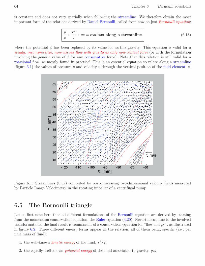
64 Chapter 6. Bernoulli equations
is constant and does not vary spatially when following the streamline. We therefore obtain the mostimportant form of the relations derived by Daniel Bernoulli, called from now on just Bernoulli equation:
p
ρ+
v2
2+ gz = constant along a streamline (6.18)
where the potential φ has been replaced by its value for earth’s gravity. This equation is valid for asteady, incompressible, non-viscous flow with gravity as only non-contact force (or with the formulationinvolving the generic value of φ for any conservative force). Note that this relation is still valid for arotational flow, as mostly found in practice! This is an essential equation to relate along a streamline(figure 6.1) the values of pressure p and velocity v through the vertical position of the fluid element, z.
Figure 6.1: Streamlines (blue) computed by post-processing two-dimensional velocity fields measuredby Particle Image Velocimetry in the rotating impeller of a centrifugal pump.
6.5 The Bernoulli triangle
Let us first note here that all different formulations of the Bernoulli equation are derived by startingfrom the momentum conservation equation, the Euler equation (4.20). Nevertheless, due to the involvedtransformations, the final result is reminiscent of a conservation equation for “flow energy”, as illustratedin figure 6.2. Three different energy forms appear in the relation, all of them being specific (i.e., perunit mass of fluid):
1. the well-known kinetic energy of the fluid, v2/2;
2. the equally well-known potential energy of the fluid associated to gravity, gz;

6 Simplification of the Bernoulli equation for a gas flow 65
kinetic energy
v2/2pressure “energy”
p/ρ
potential energy
gz
Figure 6.2: Possible exchanges between different forms of flow energy according to the Bernoulli equation(6.18).
3. as a first component, a more specific pressure “energy” of the fluid, p/ρ.
All these contributions have of course the right unit for a specific energy, i.e., J/kg. The so-calledpressure energy is the only new term; it is of course well-known that it is possible to generate work byusing a pressure difference (i.e., letting a pressure force work). But it is the first time that we associatedirectly with the absolute pressure p in the fluid a contribution similar to a specific energy.Beware! Please note that the possible exchanges between the three different forms of flow energyillustrated in figure 6.2 are still associated with limitations! We will always assume in practice that thelowest vertical position in the considered flow is associated with z = 0 per convention. This means thatthe upper term in figure 6.2 (potential energy), is always positive: gz ≥ 0. It is furthermore obviousthat the kinetic energy term on the right is also positive: v2/2 ≥ 0. Finally, the pressure term on theleft is also positive since pressure p and density ρ are both positive: p/ρ ≥ 0. As a consequence, whenequation (6.18) is used to illustrate the possible exchange between potential energy, kinetic energy andpressure energy, it must be kept in mind that, during the exchange process, all three terms must alwaysremain positive! A flow for which one or more of these contributions would be negative is physicallyimpossible to realize.
Concerning the pressure term, the real physical condition is even more stringent, p/ρ > 0, due to aphenomenon called cavitation.
6.6 Simplification of the Bernoulli equation for a gas flow
To illustrate this point, let us compare the order of magnitude of the first term (pressure energy) andof the last term (potential energy) for a non-flowing flow (static conditions, see equation 6.14).
Considering for example a water height H of 10 m, we have demonstrated in Chapter 5 that theresulting hydrostatic overpressure is ρgH ≈ 1 bar (with ρ = 1000 kg/m3). It has therefore the same orderof magnitude as the atmospheric pressure and as pressure levels found in most practical applications. Ifwe now consider the same term for an air column, neglecting any change in density, the resulting staticoverpressure is ρgH ≈ 0.001 bar (with ρ = 1.2 kg/m3), hence roughly thousand times smaller.
This simple example illustrates the fact that, when using the Bernoulli equation for a gas flow, thelast term in equation (6.18) can usually safely be neglected compared to the other contributions. Theonly exceptions would be cases where both gas pressure and gas velocity are extremely small, or whenconsidering huge variations of the z-coordinate (a gas column of several kilometers, for example in an

66 Chapter 6. Bernoulli equations
atmospheric application). For all other standard engineering conditions, the Bernoulli equation for anincompressible gas flow can be simplified as:
p
ρ+
v2
2= constant along a streamline (6.19)
6.7 Dynamic pressure
It is of course possible to multiply the Bernoulli equation (6.18) with the fluid density ρ, leading to:
p+ρv2
2+ ρgz = constant along a streamline (6.20)
Obviously, all three terms in this equation have the same unit, the unit of pressure (Pascal, Pa). Morespecifically, the second term in this equation, ρv2/2 will from now on also be called dynamic pressure q:
q :=ρv2
2(6.21)
If we neglect the contribution of potential energy, the meaning of this dynamic pressure is clear: startingfrom a flow with conditions p for pressure and v for velocity, if this flow is decelerated until coming torest (i.e., v = 0, called stagnation conditions) the pressure will simultaneously increase by an amountequal to the initially available dynamic pressure. This is illustrated in Table 6.1.
v −→ 0
p −→ p +ρv2
2
Table 6.1: Change of flow pressure and flow velocity from starting conditions to stagnation conditions
6.8 Averaged Bernoulli equation
We have already seen two possible formulations of the Bernoulli equation. The first one (equation 6.12)would be extremely useful, but is only valid for irrotational flows and is therefore of limited application.The second one, equation (6.18) can be applied for a variety of flows, but can only be used when aspecific streamline has been determined. Identifying such a streamline is a tedious process and it cansometimes be a complex issue. Would it be possible to compromise between the two formulations, sothat we could use an equation similar to equation (6.12) even for a rotational flow?
This is indeed possible for internal flows, for which the formulation to come will be particularly useful.For this purpose, we consider an incompressible flow within a pipe of arbitrary geometry (the cross-section area A may vary in an arbitrary manner, the pipe direction can change freely along horizontaland vertical coordinates).
We keep the standard assumptions used at the beginning of this chapter: the flow is steady,incompressible, non-viscous, with gravity as only non-contact force (or with the formulation involv-ing the generic value of the potential φ for any conservative force). It is therefore possible to use readilyequation (6.18) as long as a suitable streamline has been identified for this purpose. Now, instead ofconsidering the full flow, we limit the analysis to the variation between an inflow cross-section A1 and

8 Averaged Bernoulli equation 67
an outflow cross-section A2 (figure 6.3). The identified streamline will connect (in an unknown manner)the inflow and the outflow cross-section. Along this streamline, we might write equation (6.18):
p
ρ+
v2
2+ gz = constant (6.22)
or considering only the initial conditions (index 1) and final conditions (index 2) along this streamline:
p1ρ
+v1
2
2+ gz1 =
p2ρ
+v2
2
2+ gz2 (6.23)
It is in principle possible to repeat this process for all streamlines in this flow, therefore connecting allfluid elements present along the inflow cross-section A1 with their corresponding state along the outflowcross-section A2 (figure 6.3).
A1 A2
Figure 6.3: Averaging procedure between inflow and outflow cross-sections.
If we now average in space along the cross-section all corresponding equations, we obtain the averagedBernoulli equation:
p1ρ
+v21
2+ gz1 =
p2ρ
+v22
2+ gz2 (6.24)
where the indices 1 and 2 characterize again respectively the inflow and outflow cross-sections, A1 andA2, and where the symbols with overline correspond to spatially-averaged values along the correspondingcross-section, for example:
p1 :=1
A1
∫ ∫
A1
p(x)dA (6.25)
If the flow is indeed one-dimensional along the inflow and outflow cross-sections, A1 and A2, thenthis averaging procedure is superfluous for flow pressure and flow velocity. In such a case, the pressureand the velocity are constant along a cross-section, so that p1 = p1, v2
1 = v21, p2 = p2 and v2
2 = v22.
Nevertheless, even in such a case, the vertical coordinate z must still be averaged (z1 6= z1), exceptin the case where the pipe is running purely along the vertical direction, so that each cross-sectioncorresponds to a plane z = constant. In general, z is simply the z-coordinate of the geometrical centerof the corresponding pipe cross-section. For a circular pipe, this will be the value of z associated withthe pipe axis.
From now on, we will write the averaged Bernoulli equation without the overlines, leading simply to:
p1ρ
+v21
2+ gz1 =
p2ρ
+v22
2+ gz2 (6.26)
associated with following conditions:

68 Chapter 6. Bernoulli equations
1. this equation is valid between an inflow cross-section A1 and an outflow cross-section A2;
2. all terms appearing in this equation have been spatially averaged along each cross-section followingequation (6.25); or alternatively the flow is one-dimensional along the inflow and outflow cross-sections and the value of z appearing in the equation is the z-coordinate of the geometric centerof the corresponding cross-section;
3. as usual, the flow is steady, incompressible, non-viscous, with gravity as only non-contact force(or with the formulation involving the generic value of the potential φ for any conservative force).
On the other hand, it is not necessary to have an irrotational flow in order to apply equation (6.26).And it is also not necessary to identify any streamline before using this equation!
Since the boundary of a streamtube cannot be crossed by any fluid particle, a streamtube is closelysimilar to the internal flow within a duct of variable cross-section (that of the streamtube), as consideredup to now. The results presented in this section for an internal flow can therefore equally well be appliedto any streamtube, as long as the assumptions listed above are valid. Of course, in that case, it is yourresponsibility to identify correctly the streamtube before applying equation (6.26) between the inflowand outflow cross-sections.
Beware! If you have the feeling that you have been cheated during the developments presented inthis section, you are quite right! From a purely mathematical point of view, the so-called “averagingprocess” introduced to develop equation (6.26) is certainly not a clean proof. . . It is indeed possible (butrelatively difficult) to prove that equation (6.26) is perfectly correct. The corresponding proof will beadded in a later version of this document.
6.9 Hydraulic height
Equation (6.26) can be equally well rewritten by dividing everything with the gravity acceleration g,leading to:
p1ρg
+v21
2g+ z1 =
p2ρg
+v22
2g+ z2 (6.27)
Obviously, all terms in this equation have now the same unit as z, i.e., meter (m). All can therefore bewritten as equivalent lengths. The sum of all three terms, being constant as shown by this equation, iscalled from now on hydraulic head (sometimes also total head) and is written H :
H :=p
ρg+
v2
2g+ z = constant (6.28)
The three terms building up the (constant) hydraulic head are the pressure head p/(ρg), the dynamic(or velocity) head v2/2g and the elevation (or geodetic) head z. All these terms are expressed in meters.It is now possible to use equation (6.28) to analyze graphically the evolution of the flow properties in apractical installation, as shown schematically in figure 6.4. As already explained previously, it must ofcourse be kept in mind that all three separate contributions (elevation head, dynamic head and pressurehead) must always remain positive: this is obvious for the dynamic head; it is the result of the chosenconvention (z = 0 at the lowest point in the flow) for the elevation head; and it is even more stringent(p/(ρg) > 0) for the pressure head due to cavitation.

10 Generalized Bernoulli equation with losses and energy exchange 69
velocity/dynamic head v1
2/(2g)
pressure head p1/( g)
elevation head z1
“0” level
hydraulic or total head H
1 2
velocity/dynamic head v2
2/(2g)
pressure head p2/( g)
elevation head z2
hhhhyddddraulic or total head H
1
2
Figure 6.4: Graphical representation of a possible evolution for pressure head, dynamic head and eleva-tion head for a constant total head and a constant pipe diameter (hence constant velocity v).
6.10 Generalized Bernoulli equation with losses and energy
exchange
It is now possible, based on the previously introduced averaged Bernoulli equation (6.26), to present thelast and most complete form of the relations associated with Daniel Bernoulli.
The purpose of this last formulation that we will later call generalized Bernoulli equation, is inparticular to take into account the influence of all kinds of losses found in practical flows. Up to now,these losses have been completely neglected and therefore do not appear at all in equation (6.26). Inpractice such losses might be of considerable importance and have two main origins:
1. they might be a result of friction, whenever velocity gradients are found in a flow. This is usuallythe case in practice, and such velocity gradients can be particularly large near the walls, in theboundary layer.
2. they might be the result of other flow modifications leading to an irreversible change of thermo-dynamic state. This is also very often the case, for instance when changing rapidly flow directionor velocity magnitude, or within vortices, as encountered in bends, reducers, junctions, at theentrance of exit or a pipe, within a valve. . .
Globally, all these losses correspond to an entropy increase. In order to quantify them exactly, a

70 Chapter 6. Bernoulli equations
conservation equation for energy and entropy in the flow would be needed, together with a detailedanalysis of the local flow conditions in time and space. Even if this is possible in practice, this is toocomplex for our present level of knowledge and for most practical applications.
Therefore, our purpose is now simply to model such losses in an appropriate manner, allowing asufficiently accurate (but not exact) determination of the resulting flow properties.
As we already know, there are three different possible units that can be used to write the averagedBernoulli equation: either all quantities are expressed as equivalent to pressure (unit: Pa), equivalentto geodetic height (unit: m) or equivalent to specific energy (unit: J/kg). Equivalently, the head lossappearing in the flow can be expressed as:
• equivalent energy loss (or dynamic head loss), written ∆e and measured in J/kg.
• equivalent pressure loss (or pressure head loss), written ∆p and measured in Pa.
• equivalent geodetic height loss (or elevation head loss), written ∆z and measured in m.
Per convention, all these losses will be considered as positive. It is of course very easy to convert oneexpression to the other, using:
∆z =∆p
ρg=
∆e
g(6.29)
If we now write with an index f the losses associated to friction and with an index l all other losses (ldesignates here a “localized” loss, since such a loss can be associated to a specific location in the flow;note, however, that these losses are most commonly called “minor losses” in the international literature,a somewhat misleading name, since they might indeed be quite large). Now, the friction loss (consideredglobally for the complete flow) and a number of localized losses (numbered 1 to n in what follows, andassociated to localized flow modifications), can be taken into account in the Bernoulli equation, leadingto: [
p2ρ
+v22
2+ gz2
]
=
[
p1ρ
+v21
2+ gz1
]
−∆ef −n∑
j=1
∆el,j (6.30)
or equivalently[
p2ρg
+v22
2g+ z2
]
=
[
p1ρg
+v21
2g+ z1
]
−∆zf −n∑
j=1
∆zl,j, (6.31)
[
p2 +ρv2
2
2+ ρgz2
]
=
[
p1 +ρv2
1
2+ ρgz1
]
−∆pf −n∑
j=1
∆pl,j (6.32)
Since we will always encounter such losses in practical flows, we must find a solution to compensatethem. This is simply realized by exchanging work with the fluid. If the user wants to increase the energylevel of the fluid, it will communicate work to it, typically using a pump, delivering a positive specificwork w > 0 to the fluid. Conversely, if the fluid is used to generate energy, the negative work w < 0will be lost by the fluid and communicated to the surroundings, usually using a turbine. As you see, theexchanged specific work w (expressed in J/kg) is always considered from the point of view of the fluid;it is positive when increasing fluid energy, negative when fluid energy is reduced. Finally, if a certainnumber m of such devices exchanging work with the fluid are found between the inflow cross-section A1
and the outflow cross-section A2, the generalized Bernoulli equation can be written:
[
p2ρ
+v22
2+ gz2
]
−[
p1ρ
+v21
2+ gz1
]
=m∑
i=1
wi −∆ef −n∑
j=1
∆el,j (6.33)
and is associated with following conditions:

10 Generalized Bernoulli equation with losses and energy exchange 71
1. all terms appearing in this equation have been spatially averaged along inflow and outflow cross-sections following equation (6.25); or alternatively the flow is one-dimensional along the inflowand outflow cross-sections and the value of z appearing in the equation is the z-coordinate of thegeometric center of the corresponding cross-section;
2. the flow is steady, incompressible, with gravity as only non-contact force (or with the formulationinvolving the generic value of the potential φ for any conservative force).
On the other hand, it is now not necessary to have a non-viscous flow, since the influence of viscouslosses appears in the equation (∆ef )! This equation can readily be used for a rotational flow, and it isnot necessary to identify any streamline before using this relation.
In order to solve any practical problem, the only remaining issue is now to determine exactly all termson the right-hand side, since the left-hand side is well-known, involving only classical contributions.
6.10.1 Computing the exchanged specific work w
The specific work w exchanged between the fluid and the surroundings is mostly well-known; it willbe simply regulated by the user (for a pump, delivering a positive specific work wp) or measured as anoutput quantity by the user (for a turbine, delivering to the surroundings a positive specific work wt).If the efficiency η of the apparatus is 100%, the relation between the value set/read by the user andthe value relevant for the fluid and appearing in equation (6.33) is simply w = wp for a pump, resp.w = −wt for a turbine.
In reality, the efficiency η of the apparatus is not perfect, η < 1. For a pump with an efficiency ηp,the real relation between the work of the pump and the final amount really available for increasing fluidenergy is then:
w = ηpwp (6.34)
Conversely, for a turbine with an efficiency ηt, the relation between the amount of energy lost by thefluid and the energy really available for the turbine user reads:
w =wt
ηt(6.35)
If needed, the relation between specific work w and associated power P is simply:
P = mw (6.36)
6.10.2 Computing the friction loss ∆ef
Remember that we are looking for an acceptably accurate estimation of the losses occuring in practice insuch a flow and not for an exact solution. As a consequence, the underlying methodology relies mostlyon systematic experimental measurements, supported as far as possible by theoretical considerationsleading to major simplifications. The corresponding theory and the resulting complexity reduction willbe described later (Chapter 10); we now concentrate only on the information obtained from experimentalstudies.
From a fundamental point of view, the formulation of the generalized Bernoulli equation written asa specific energy equation (6.33) is most appropriate, and will be used in what follows. Nevertheless,you can easily convert the resulting losses as equivalent pressure head loss or elevation head loss usingequation (6.29):
∆z =∆p
ρg=
∆e
g(6.37)

72 Chapter 6. Bernoulli equations
As we will discuss later, friction is indeed a result of gradients of flow momentum (or equivalently,for an incompressible flow as considered here, gradients of flow velocity). There is therefore a resultingconnection between friction loss ∆ef and flow velocity v. As a consequence, it is very practical to expressthe friction loss as a function of the available specific kinetic energy in the flow, v2/2.
Finally, the measured friction loss depends of course on the considered flow configuration. Qualita-tively, since we have stated previously that velocity gradients will be particularly large near the walls,in the so-called boundary layer, the importance of friction loss will be considerable for flows in contactwith “a lot of” walls (micro-channels, heat exchangers) and quite negligible in the opposite case (smoothstraight tube with a very large diameter, without any insert).
In practice, cylindrical pipes are mostly encountered. Therefore, we will only give here results forsuch a configuration: a straight cylindrical pipe of length l, diameter d, with a mean axial flow velocity v.Systematic experiments show that the associated friction loss can be computed using following relation,called Darcy-Weisbach equation:
∆ef = fl
d
v2
2(6.38)
where the dimensional parameter f appearing in this equation is called friction factor, as first introducedby Darcy in the 19th century after carrying out a large amount of pipe flow measurements.
Apart from f , all quantities in this equation are already known (note that the norm of the flowvelocity ‖ v ‖= v will in practice mostly be computed from the volumetric flow-rate, equation (1.5),using v = q/A).
The friction factor has been measured experimentally in a highly systematic manner for a variety ofconfigurations. Corresponding contributions, mainly by Darcy, Weisbach, Nikuradse and Moody finallylead to an expression of the friction factor depending from the Reynolds number Red of the flow andfrom the relative wall roughness height ǫ/d:
f = f(
Red,ǫ
d
)
(6.39)
The Reynolds number will be discussed in detail in Chapter 10. Let us simply define it here. It is anon-dimensional number computed as:
Red :=ρvd
µ=
vd
ν(6.40)
where the dynamic viscosity µ or kinematic viscosity ν can be equally well employed, taking into accountthe relation ν = µ/ρ.
The functional dependency described by equation (6.39) is summarized in a well-known graphicalrepresentation, called Moody chart (or Moody-Colebrook chart) (figure 6.5). The resulting value of thefriction factor is always well below unity (typically, f < 0.1).
Now, the final procedure to compute friction loss ∆ef in a straight cylindrical pipe is clear. First, themean velocity v must be known or computed, together will all geometrical characteristics including thewall roughness height ǫ, a measure of the “smoothness” of this wall. Then, it is possible to compute theReynolds number Red from equation (6.40) and the relative wall roughness height ǫ/d. A large value ofǫ/d means a very rough wall (pipe of bad quality), while a small value of ǫ/d means a higher smoothnessand therefore lower friction loss (it is clear from figure 6.5 that f , and therefore ∆ef , increases withǫ/d).
Knowing these two values, figure 6.5 is employed to determine f . The value of the friction factor isthen used in equation (6.38) in order to compute the final value of ∆ef .
Finally, remember that this procedure is just a sufficiently accurate approximation of the reality. Thevalue of f employed in the computation is probably not so accurate (an error of a few % is considered

10 Generalized Bernoulli equation with losses and energy exchange 73
as fully acceptable). And the value of ǫ entering the computation is not that well-known, may varyspatially or in time (corrosion, particle deposition on the walls). The friction loss you determine in thismanner is only a relatively accurate estimation.
If the considered pipe is not a standard, cylindrical pipe, it is still possible to use the results pre-sented in this section by replacing everywhere and in a systematic manner the diameter d by thehydraulic diameter dh. This leads to an even higher error level, but allows to consider an arbitrarygeometry.
6.10.3 Numerical equations used to estimate the friction factor f
Usually, using the Moody-Colebrook chart diagram as described in the previous section in order todetermine graphically the solution is fully sufficient. But, for solving practical problems, an equationgiving (directly or indirectly) the value of f would be much more practical and/or would speed-upconsiderably the solution procedure. Many such fitting laws are available.
Friction factor f in the laminar regime
For laminar flow conditions, which means in practice for a value of the hydraulic Reynolds number Redbelow roughly 2 300 for an axisymmetric pipe (top-left part of the Moody-Colebrook chart), we willshow later in Chapter 9 that an exact formula can be obtained for such conditions, reading simply:
f =64
Red(6.41)
Approximation of the friction factor f for smooth conditions
Here, different formulas are found, which are simply fitting more or less accurately the experimentalmeasurement represented in the Moody-Colebrook chart diagram.
• For 4 000 ≤ Red ≤ 105, the law of Blasius is mostly employed and gives directly the value of f :
f = 0.3164 Red−1/4 (6.42)
• For Red > 2 300, the (implicit) relation of Prandtl-Karman can be used instead, usually requiringiterations to identify f :
1√f= 2 log
(√
f Red
)
− 0.8 (6.43)
• For highly turbulent conditions (Red > 105), the direct relation of Nikuradse can be used instead:
f = 0.0032 + 0.221 Red−0.237 (6.44)
Approximation of the friction factor f for rough conditions
Here again, different formulas are found, which are simply fitting more or less accurately the experimentalmeasurement represented in the Moody-Colebrook chart.
• For Red > 2 300, the law of Colebrook-White is giving the best approximation, but is an implicitrelation and will therefore usually require iterations:
1√f= −2 log
(
2.51√f Red
+ǫ
3.7d
)
(6.45)

74 Chapter 6. Bernoulli equations
• With a slightly lower precision, but allowing a direct estimation of f , the law of Swamee-Jain canbe used instead:
f = 0.25
[
log
(
5.74
Re0.9d
+ǫ
3.7d
)]−2
(6.46)
6.10.4 Computing a localized loss ∆el
Once again, we are looking for an acceptably accurate estimation of this loss and not for an exact solution.As a consequence, the underlying methodology relies almost exclusively on systematic experimentalmeasurements.
Since localized losses are mostly somehow connected to the flow velocity v, and in order to stay asclose as possible to the friction loss considered in the previous section, it is very practical to expressagain the localized loss as a function of the available specific kinetic energy in the flow, v2/2.
Finally, the measured friction loss depends of course on the considered flow configuration and on theorigin of the considered loss. The practical computation involves simply a loss coefficient (sometimes alsocalled resistance coefficient) K, as simple proportionality coefficient between the loss and the availablespecific kinetic energy:
∆el = Kv2
2(6.47)
The value of K is given by an experimental measurement. Note that this non-dimensional valuemight well exceed unity. Available technical documents contain thousands of measurement results,corresponding to a huge variety of specific configurations. The only real difficulty for an engineer is tofind a reliable source of information corresponding exactly to the considered flow configuration.
Now, the final procedure to compute local loss ∆el is clear. First, the mean velocity ‖ v ‖= vmust be known or computed. Knowing the flow configuration and the geometry, the value of the losscoefficient K is found in a reference document. Then, equation (6.47) is employed in order to computethe final value of ∆el.
A few selected examples of localized loss coefficients K are listed in Table 6.2. Once again, thesevalues should definitely not be regarded as very accurate, but as mere approximations.

10 Generalized Bernoulli equation with losses and energy exchange 75
Configuration KTee, flanged, line flow 0.1− 0.2Tee, flanged, branched flow 0.5− 1.0Union, threaded ≈ 0.08Elbow, flanged regular 90 0.3− 0.5Return bend, flanged 180 ≈ 0.2Globe valve, fully open 6− 10Angle valve, fully open ≈ 2Gate valve, fully open ≈ 0.15Gate valve, 1/4 closed ≈ 0.26Gate valve, 1/2 closed ≈ 2.1Gate valve, 3/4 closed ≈ 17Diaphragm valve, open ≈ 2.3Diaphragm valve, half open ≈ 4.3Diaphragm valve, 1/4 open ≈ 21Water meter ≈ 7
Table 6.2: Loss coefficient K for some selected configurations

76 Chapter 6. Bernoulli equations
Figure 6.5: Approximate Moody chart based on the Swamee-Jain equation as drawn by S. Beck and R.Collins, University of Sheffield, reprinted from Wikipedia.

Chapter 7
Force and torque exerted by a flow
7.1 Introduction
In the previous chapter we have mainly considered the local evolution of the main flow variables (pressurep and velocity v). Building on top of these results, it is now possible to determine the force and thetorque exerted by such a flow on its surroundings, considering a volume of fluid limited by an inflowcross-section A1 and an outflow cross-section A2; the side surface (i.e., either the wall of the pipecontaining this flow or the corresponding outside surface of the associated streamtube) will be writtenΣ. Considering this configuration (figure 7.1), the surface constituted by assembling A1,A2 and Σ is afixed, closed surface in the fluid (Acf = A1 ∪ A2 ∪ Σ) and can be used to define a fixed control volumeVcf , contained within the surface Acf and always filled up with fluid.
n1
Outer surface Σ
Control volume V
n
n
v1
A1
A2
v2
s1
s2
n2
p1
p2
ρ2
ρ1
Figure 7.1: Configuration to compute the force exerted by a flow on the side boundary Σ.
In order to compute the force and torque exerted by the corresponding flow, we will only considersteady flow conditions, so that all flow variables are constant in time. As a supplementary assumption,we will consider only one-dimensional flows along the inflow and outflow cross-sections, A1 and A2.Furthermore, we will consider first only non-viscous flows (but we will later show that the obtainedresults are equally valid for viscous flows!).
77

78 Chapter 7. Force and torque exerted by a flow
Beware! The results obtained in this Chapter do not require at all an incompressible flow. The densityρ of the fluid may change in any manner (or stay constant), this will not affect the results presentedlater in this Chapter. This is one further attractive feature of the findings presented in what follows:they stay equally valid for a variety of different flow configurations.
7.2 Force exerted by a flow on its surroundings
In order to compute first the resulting force, we start from the integral formulation of momentumconservation for a steady flow introduced in Chapter 4 for a fixed control volume Vcf , Eq.(4.17).
∫ ∫
Acf
ρ(x, t)v(x, t) (v(x, t) · n) dA =∫ ∫ ∫
Vcf
ρ(x, t)gdV −∫ ∫
Acf
p(x, t)ndA (7.1)
Remember that Acf = A1 ∪ A2 ∪ Σ, so that each corresponding integral on Acf can be written as thesum of three integrals on A1, A2 and Σ respectively. We will also use, as already done several timespreviously in the Chapters 3 to 6, the unit vectors n (perpendicular to the local external surface Acf
and pointing toward the outside, appearing already in Eq.(7.1) and s (colinear, i.e., parallel to the localflow velocity v). From the geometrical construction of the control volume Vcf , it can easily be seenthat along the inflow cross-section A1 one obtains n1 = −s1, while along the outflow cross-section A2,n2 = s2.
The last integral involving the pressure force in Eq.(7.1) can now be rewritten as∫ ∫
Acf
p(x, t)ndA =∫ ∫
Σp(x, t)ndA+
∫ ∫
A1
p(x, t)ndA+∫ ∫
A2
p(x, t)ndA (7.2)
The first term on the right-hand side of this equation (integration over the side section Σ) is directly thepressure force exerted by the fluid on its surroundings, denoted from now on Fp: this is exactly whatwe want to determine here!
The second term can be easily computed, since the flow has been assumed one-dimensional alongthe inflow cross-section A1, leading to:
∫ ∫
A1
p(x, t)ndA =∫ ∫
A1
p1n1dA (7.3)
= p1n1
∫ ∫
A1
dA (7.4)
= p1n1A1 (7.5)
= −p1s1A1 (7.6)
where A1 is the area of A1. In the same manner, the last integral in Eq.(7.2) can be written:∫ ∫
A2
p(x, t)ndA = p2n2A2 (7.7)
= p2s2A2 (7.8)
with A2 the area of A2. Finally, one gets:∫ ∫
Acf
p(x, t)ndA = Fp − p1s1A1 + p2s2A2 (7.9)
Following a similar technique, the first integral on the left-hand side in Eq.(7.1) can be split intothree parts:
∫ ∫
Acf
ρ(x, t)v(x, t) (v(x, t) · n) dA =

2 Force exerted by a flow on its surroundings 79
∫ ∫
Σρ(x, t)v(x, t) (v(x, t) · n) dA
+∫ ∫
A1
ρ(x, t)v(x, t) (v(x, t) · n) dA
+∫ ∫
A2
ρ(x, t)v(x, t) (v(x, t) · n) dA (7.10)
Along Σ (the pipe wall or the side section of a streamtube), one observes necessarily a flow velocity vlocally tangential to Σ (the flow cannot cross in any manner the surface Σ). As a consequence, the flowvelocity v (parallel to Σ) and the normal vector n (normal to Σ) are perpendicular to each other. Due tothe fundamental properties of the scalar product, the corresponding contribution is then automatically0: ∫ ∫
Σρ(x, t)v(x, t) (v(x, t) · n)
︸ ︷︷ ︸
=0
dA = 0 (7.11)
Along the inflow cross-section A1, the one-dimensional assumption leads again to∫ ∫
A1
ρ(x, t)v(x, t) (v(x, t) · n) dA =∫ ∫
A1
ρ1v1 (v1 · n1) dA (7.12)
= ρ1v1 (v1 · n1)∫ ∫
A1
dA (7.13)
= ρ1v1 (v1 · n1)A1 (7.14)
Since v1 = v1s1 = −v1n1, this can be rewritten:∫ ∫
A1
ρ(x, t)v(x, t) (v(x, t) · n) dA = ρ1v1s1(−v1)A1 (7.15)
= −ρ1v21s1A1 (7.16)
= −m1v1s1 (7.17)
introducing the mass flow-rate in the inflow cross-section A1, m1 = ρ1v1A1. Similarly, one obtains alongthe outflow cross-section A2,
∫ ∫
A2
ρ(x, t)v(x, t) (v(x, t) · n) dA = m2v2s2 (7.18)
Since the flow is steady, mass conservation implies the conservation of the mass flow-rate in any cross-section, so that
m1 = m2 = m (7.19)
One can therefore write finally:∫ ∫
Acf
ρ(x, t)v(x, t) (v(x, t) · n) dA = −mv1s1 + mv2s2 (7.20)
The first integral on the right-hand side of Eq.(7.1), describing the influence of gravity, can be veryeasily computed in a direct manner, remembering that the acceleration vector g can be assumed to beconstant for practical applications on the earth’s surface:
∫ ∫ ∫
Vcf
ρ(x, t)gdV = g∫ ∫ ∫
Vcf
ρ(x, t)dV (7.21)
= Mg (7.22)
where M is the total mass of the fluid contained within the fixed control volume Vcf , as already shownin Eq.(3.1).

80 Chapter 7. Force and torque exerted by a flow
Finally, it is possible to rewrite now Eq.(7.1) as:
− mv1s1 + mv2s2 = Mg − Fp + p1s1A1 − p2s2A2 (7.23)
This can now be transformed in a suitable manner to determine Fp:
Fp = (mv1 + p1A1) s1 − (mv2 + p2A2) s2 +Mg (7.24)
We define a new scalar quantity along each cross-section A in the flow, called impulsion, written F andexpressed in N (like a force), by:
F := mv + pA (7.25)
It is then possible to give the expression of the force exerted by the fluid on its surroundings throughthe separation surface Σ as:
Fp = F1s1 −F2s2 +Mg (7.26)
This relation giving the total force exerted by the fluid between the inflow cross-section A1 and outflowcross-section A2 is valid for a steady non-viscous flow, assumed moreover one-dimensional along theinflow and outflow cross-sections, A1 and A2.
It must be noticed here that the force exerted by a volume of fluid (that contained within the fixedcontrol volume Vcf) can be computed by knowing only the main flow parameters in the inflow andoutflow cross-sections (change of impulsion F and/or of flow direction s); it is not necessary to know thedetails of the flow within Vcf , only start and end flow conditions are sufficient to compute the resultingforce. This is an extremely powerful formulation, and it can be used to obtain a wealth of essentialresults in practical applications!
Note that, for most practical cases, the contribution associated to the weight of the fluid (Mg, lastterm in Eq.7.26) can usually be safely neglected when considering a gas flow, since gas densities are quitelow. On the other hand, it must be taken into account for a liquid, since it might lead to considerablevalues.
At the present level, the results of Eq.(7.26) are equally valid for the flow in a pipe (pipe wall Σ) orfor the flow within a streamtube, in which case Σ is just a geometrical surface in the fluid separating ina purely theoretical manner different fluid elements.
7.3 Force exerted by a flow on a pipe wall surrounded by a
fluid at constant pressure
If we now consider more specifically an internal flow in a pipe, Σ is the pipe wall surrounding the fluid.In most practical cases, outside of the pipe, a constant pressure p = pa is found everywhere (figure 7.2).When trying to compute the resulting force on the pipe wall, it is more useful in practice to take intoaccount as well the influence of the external pressure, pa, and not only the action of the internal fluidpressure, as done in the previous section.
The force exerted by the internal flow on the pipe wall, Σ, has been determined in the previoussection and is given by Eq.(7.26).
The supplementary pressure force exerted by the constant and homogeneous external pressure pa onthe same wall is now:
Fpa = −∫ ∫
ΣpandA (7.27)
where the minus sign denotes the fact that this pressure force is acting towards the inside of the controlvolume, i.e., towards −n.

3 Force exerted by a flow on a pipe wall surrounded by a fluid at constant pressure 81
n1
Outer surface Σ
Control volume V
n
n
v1
A1
A2
v2
s1
s2
n2
p1
p2
ρ2
ρ1
pa
pa
pa
pa
Figure 7.2: Configuration to compute the force exerted by a flow on the pipe wall Σ taking into accountthe constant and uniform external pressure pa.
Let us consider the same integral but integrating now over the complete, closed outer surface of theconsidered, fixed control volume Vcf , i.e., the surface Acf = A1 ∪A2 ∪ Σ.
One gets first:∫ ∫
Acf
pandA = pa
∫ ∫
Acf
ndA (7.28)
Now, using the second formulation of the divergence theorem (Eq. C.6), it is possible to replace this lastintegral, leading to: ∫ ∫
Acf
ndA =∫ ∫ ∫
Vcf
(∇1)dV (7.29)
Obviously, the gradient of a constant scalar (here 1) is zero. This demonstrates a well-known result:when integrating the normal unit vector n over any closed geometrical surface, one obtains alwaysidentically 0. Finally, this demonstrates that:
∫ ∫
Acf
pandA = 0 (7.30)
=∫ ∫
ΣpandA+
∫ ∫
A1
pandA+∫ ∫
A2
pandA (7.31)
Or−∫ ∫
ΣpandA =
∫ ∫
A1
pandA +∫ ∫
A2
pandA (7.32)
Finally, the total pressure force exerted simultaneously by the internal flow and by the external pressurepa, written in what follows Fp,pa, reads:
Fp,pa = F1s1 − F2s2 +Mg −∫ ∫
ΣpandA (7.33)
= F1s1 − F2s2 +Mg +∫ ∫
A1
pandA+∫ ∫
A2
pandA (7.34)
= F1s1 +∫ ∫
A1
pandA− F2s2 +∫ ∫
A2
pandA+Mg (7.35)

82 Chapter 7. Force and torque exerted by a flow
= F1s1 + pan1
∫ ∫
A1
dA− F2s2 + pan2
∫ ∫
A2
dA+Mg (7.36)
= F1s1 + pan1A1 − F2s2 + pan2A2 +Mg (7.37)
= (F1s1 − paA1s1)− (F2s2 − paA2s2) +Mg (7.38)
Introducing now along each cross-section A in the flow the relative impulsion, written F ′ and ex-pressed in N (like a force), by:
F ′ := mv + (p− pa)A (7.39)
it is then possible to give the expression of the force exerted by the internal fluid on the pipe wall Σtaking into account the external pressure pa by:
Fp,pa = F ′1s1 − F ′
2s2 +Mg (7.40)
This relation is valid for a steady non-viscous flow, assumed moreover one-dimensional along the inflowand outflow cross-sections, A1 and A2.
Note that, for most practical cases, the contribution associated to the weight of the fluid (Mg, lastterm in Eq.7.40) can be safely neglected when considering a gas flow, since gas densities are quite low.
7.4 Torque exerted by a flow on its surroundings
We will now compute the resulting torque exerted by a flow on its separation surface Σ (figure 7.3) byreference to a pivot P.
In order to compute the resulting torque, we start from the integral formulation of angularmomentumconservation for a steady flow introduced in Chapter 4 for a fixed control volume Vcf , Eq.(4.26):
∫ ∫
Acf
r× [ρ(x, t)v(x, t) (v(x, t) · n)] dA =
∫ ∫ ∫
Vcf
r× [ρ(x, t)g] dV −∫ ∫
Acf
r× [p(x, t)n] dA (7.41)
Remember that Acf = A1∪A2∪Σ, so that each corresponding integral on Acf can be written as the sumof three integrals on A1, A2 and Σ respectively. Here, we employ again the unit vector n (perpendicularto the local external surface Acf and pointing toward the outside, appearing already in Eq.7.41) and s(colinear, i.e., parallel to the local flow velocity v). From the geometrical construction of the controlvolume Vcf , it can easily be seen that along the inflow cross-section A1 one obtains n1 = −s1, whilealong the outflow cross-section A2, n2 = s2.
The last integral involving the pressure force in Eq.(7.41) can now be rewritten as∫ ∫
Acf
r× [p(x, t)n] dA =
∫ ∫
Σr× [p(x, t)n] dA+
∫ ∫
A1
r× [p(x, t)n] dA+∫ ∫
A2
r× [p(x, t)n] dA (7.42)
The first term on the right-hand side of this equation (integration over the side section Σ) is directlythe torque exerted by the fluid pressure on its surroundings, denoted from now on Tp: this is what wewant to determine here!
The second term can be easily computed, since the flow has been assumed one-dimensional alongthe inflow cross-section A1, leading to:
∫ ∫
A1
r× [p(x, t)n] dA =∫ ∫
A1
r× [p1n1] dA (7.43)

4 Torque exerted by a flow on its surroundings 83
Outer surface Σ
Control volume V
v1
A1
A2
v2
s2
P
G1
G2
G
r
r1r2
s1
Figure 7.3: Configuration to compute the torque exerted by a flow on the side boundary Σ by referenceto the pivot P.
=[∫ ∫
A1
rdA]
× (p1n1) (7.44)
= −[∫ ∫
A1
rdA]
× (p1s1) (7.45)
The integral appearing in this relation, leading to the mean value of r when covering all the inflowsurface A1, reads simply:
∫ ∫
A1
rdA = r1A1 (7.46)
where A1 is the area of A1 and r1 = ~PG1 is the vector connecting the pivot P with the geometricalcenter G1 of A1.
Finally, one gets:∫ ∫
A1
r× [p(x, t)n] dA = −r1 × (p1A1s1) (7.47)
In the same manner, the last integral in Eq.(7.42) can be written:
∫ ∫
A2
r× [p(x, t)n] dA = r2 × (p2A2n2) (7.48)
= r2 × (p2A2s2) (7.49)
with A2 the area of A2 and r2 = ~PG2 the vector connecting the pivot P with the geometrical center G2
of A2.

84 Chapter 7. Force and torque exerted by a flow
Finally:∫ ∫
Acf
r× [p(x, t)n] dA = Tp − r1 × (p1A1s1) + r2 × (p2A2s2) (7.50)
Following a similar technique, the first integral on the left-hand side in Eq.(7.41) can be split intothree parts:
∫ ∫
Acf
r× [ρ(x, t)v(x, t) (v(x, t).n)] dA =
∫ ∫
Σr× [ρ(x, t)v(x, t) (v(x, t).n)] dA
+∫ ∫
A1
r× [ρ(x, t)v(x, t) (v(x, t).n)] dA
+∫ ∫
A2
r× [ρ(x, t)v(x, t) (v(x, t).n)] dA (7.51)
Along Σ (the pipe wall or the side section of a streamtube), one observes necessarily a flow velocity vlocally tangential to Σ (the flow cannot cross in any manner the surface Σ). As a consequence, the flowvelocity v (parallel to Σ) and the normal vector n (normal to Σ) are perpendicular to each other. Due tothe fundamental properties of the scalar product, the corresponding contribution is then automatically0:
∫ ∫
Σr×
ρ(x, t)v(x, t) (v(x, t) · n)
︸ ︷︷ ︸
=0
dA = 0 (7.52)
Along the inflow cross-section A1, the one-dimensional assumption leads again to∫ ∫
A1
r× [ρ(x, t)v(x, t) (v(x, t) · n)] dA
=∫ ∫
A1
r× [ρ1v1 (v1 · n1)] dA (7.53)
=[∫ ∫
A1
rdA]
× (ρ1v1 (v1 · n1)) (7.54)
Since v1 = v1s1 = −v1n1, this can be rewritten:∫ ∫
A1
r× [ρ(x, t)v(x, t) (v(x, t) · n)] dA
=[∫ ∫
A1
rdA]
× (ρ1v1 (−v1)) (7.55)
= −[∫ ∫
A1
rdA]
×(
ρ1v21s1)
(7.56)
The integral appearing in this equation can be again computed using Eq.(7.46), leading finally to∫ ∫
A1
r× [ρ(x, t)v(x, t) (v(x, t) · n)] dA
= −r1 ×(
ρ1v21A1s1
)
(7.57)
= −r1 × (m1v1s1) (7.58)
introducing the mass flow-rate in the inflow cross-section A1, m1 = ρ1v1A1. Similarly, one obtains alongthe outflow cross-section A2,
∫ ∫
A2
r× [ρ(x, t)v(x, t) (v(x, t) · n)] dA
= r2 × (m2v2s2) (7.59)

4 Torque exerted by a flow on its surroundings 85
As already explained previously, since the flow is steady, mass conservation implies the conservation ofthe mass flow-rate in any cross-section, so that
m1 = m2 = m (7.60)
One can therefore write finally:∫ ∫
Acf
r× [ρ(x, t)v(x, t) (v(x, t) · n)] dA = −r1 × (mv1s1) + r2 × (mv2s2) (7.61)
in which the vectors r1 = ~PG1 and r2 = ~PG2 have been again used.The first integral on the right-hand side of Eq.(7.41), describing the influence of gravity, can be very
easily computed in a direct manner, remembering that the acceleration vector g can be assumed to beconstant for practical applications on the earth’s surface:
∫ ∫ ∫
Vcf
r× [ρ(x, t)g] dV =
[∫ ∫ ∫
Vcf
ρ(x, t)rdV
]
× g (7.62)
The integral appearing on the right-hand side (mean value of ρr over the complete fixed control volumeVcf) is precisely the integral used to define the center of mass of the fluid contained within Vcf , so that
∫ ∫ ∫
Vcf
ρ(x, t)rdV = Mrg (7.63)
where M is the total mass of the fluid contained within the fixed control volume Vcf , as already shown
in Eq.(3.1), and rg = ~PG connects the pivot P with the center of mass of the fluid within Vcf (point G).One obtains thus: ∫ ∫ ∫
Vcf
r× [ρ(x, t)g] dV = rg × (Mg) (7.64)
Finally, it is possible to rewrite now Eq.(7.41) as:
− r1 × (mv1s1) + r2 × (mv2s2) = rg × (Mg)−Tp + r1 × (p1A1s1)− r2 × (p2A2s2) (7.65)
This can now be transformed in a suitable manner to determine Tp:
Tp = r1 × [(mv1 + p1A1) s1]− r2 × [(mv2 + p2A2) s2] + rg × (Mg) (7.66)
Using again the impulsion F = mv + pA it is now possible to give the expression of the torque exertedby the fluid on its surroundings through the separation surface Σ by reference to a pivot P as:
Tp = r1 × (F1s1)− r2 × (F2s2) + rg × (Mg) (7.67)
This relation giving the total torque exerted by the fluid between the inflow cross-section A1 and outflowcross-section A2 is valid for a steady non-viscous flow, assumed moreover one-dimensional along theinflow and outflow cross-sections, A1 and A2. It is practically identical to the expression giving the totalforce, Eq.(7.26), when considering for each contribution the vector product with the associated leverarm rg (resp. r1, r2) connecting the pivot P with the corresponding center of mass G (resp. geometriccenter G1, G2)
Again, the torque exerted by a volume of fluid (that contained within the fixed control volume Vcf )can be computed by knowing only the main flow parameters in the inflow and outflow cross-sections;it is not necessary to know the details of the flow within Vcf , only start and end flow conditions aresufficient to compute the resulting torque. This is an extremely powerful formulation!

86 Chapter 7. Force and torque exerted by a flow
Note that, for most practical cases, the contribution associated to the weight of the fluid (Mg, lastterm in Eq.7.67) can usually be safely neglected when considering a gas flow, since gas densities are quitelow. On the other hand, it must be taken into account for a liquid, since it might lead to considerablevalues.
Equation (7.67) is equally valid for the flow in a pipe (pipe wall Σ) or for the flow within a streamtube,in which case Σ is just a geometrical surface in the fluid separating in a purely theoretical manner differentfluid elements.
7.5 Torque exerted by a flow on a pipe wall surrounded by a
fluid at constant pressure
If we now consider more specifically an internal flow in a pipe, Σ is the pipe wall surrounding the fluid.In most practical cases, outside of the pipe, a constant pressure p = pa is found everywhere (figure 7.4).When trying to compute the resulting torque on the pipe wall, it is more useful in practice to take intoaccount as well the influence of the external pressure, pa, and not only the action of the internal fluidpressure, as done in the previous section.
Outer surface Σ
Control volume V
v1
A1
A2
v2
s2
pa
pa
pa
P
G1
G2
G
r
r1r2
s1
Figure 7.4: Configuration to compute the torque exerted by a flow on the pipe wall Σ taking into accountthe constant and uniform external pressure pa.
The torque exerted by the internal flow on the pipe wall, Σ, has been determined in the previoussection and is given by Eq.(7.67).
The supplementary pressure torque exerted by the constant and homogeneous external pressure pa

5 Torque exerted by a flow on a pipe wall surrounded by a fluid at constant pressure 87
on the same wall is now:Tpa = −
∫ ∫
Σr× [pan] dA (7.68)
where the minus sign denotes the fact that the associated force is acting towards the inside of the controlvolume, i.e., towards −n.
The further process is completely identical to that already used in Section 7.3. Compared to theresults introduced in the previous section, the only difference obtained at the end is the fact that therelative pressure (p−pa) appears everywhere in the system of equations instead of the absolute pressurep. As in Section 7.3, this is indirectly due to the fact that the integral of the normal vector n over anarbitrary (but closed) geometrical surface (here Acf = A1 ∪ A2 ∪ Σ) is always zero.
Finally, using again the relative impulsion F ′ = mv + (p− pa)A, it is possible to give the expressionof the torque exerted by the internal fluid on the pipe wall Σ taking into account the external pressurepa by:
Tp,pa = r1 × (F ′1s1)− r2 × (F ′
2s2) + rg × (Mg) (7.69)
This relation is valid for a steady non-viscous flow, assumed moreover one-dimensional along the inflowand outflow cross-sections, A1 and A2.
Again, for most practical cases, the contribution associated to the weight of the fluid (Mg, last termin Eq.7.69) can be safely neglected when considering a gas flow, since gas densities are quite low.

88 Chapter 7. Force and torque exerted by a flow

Chapter 8
Movement of a material control volume
8.1 Introduction
In the present chapter, we will consider the infinitesimal movement of a material control volume Vcm,i.e., one control volume containing always the same fluid elements. We will decompose this movementin several elementary steps, useful to understand the global change in position and shape of such anarbitrary material control volume Vcm.
8.2 Movement of a material control volume
We consider now the infinitesimal movement of a material control volume Vcm, as represented in figure8.1. It is assumed to be of small, rectangular dimensions (dx× dy) at the initial time t0. The analysisis carried out in two dimensions (x and y directions) for the sake of simplicity. A three-dimensionalanalysis would be slightly more complex but would deliver exactly the same results.
x
y
A
D
Time t0
x
y
A
D
Time t0
Time
(t0+dt)
A
D
Figure 8.1: Configuration employed to investigate the movement of a material control volume.
We will determine the new position of this material control volume Vcm at a slightly later time,(t0 + dt). For our present purpose, it is sufficient to trace the movements of point A and of point D,
89

90 Chapter 8. Movement of a material control volume
constituting the diagonal direction. The velocity of point A, vA is assumed to be known at time t0,together with its spatial derivatives:
vA(t0) = (vAx, vAy
) (8.1)
At time t0, the position of point A is defined as (xA, yA). The movement of any point belonging tothe material control volume until the later time (t0 + dt) is the result of the fluid movement, startingfrom its initial position and following the local flow velocity. For point A at t0, one therefore obtains:
Point A time t0 → time (t0 + dt)x− coordinate xA → xA + vAx dty − coordinate yA → yA + vAy dt
(8.2)
Initially, at time t0, the point D is located at a distance (dx, dy) from point A. If we call vD its (atpresent unknown) velocity at time t0, one obtains in the same manner:
Point D time t0 → time (t0 + dt)x− coordinate xD → xD + vDx dty − coordinate yD → yD + vDy dt
(8.3)
Since xD = xA + dx and yD = yA + dy, this can be rewritten:
Point D time t0 → time (t0 + dt)x− coordinate xA + dx → xA + dx+ vDx dty − coordinate yA + dy → yA + dy + vDy dt
(8.4)
Now, how is it possible to determine, at least in an approximate manner, the velocity vD at point D?Since the dimensions (dx, dy) have been assumed very small, this is readily possible using a Taylor expansion,since we know the flow velocity and its derivatives at point A! Retaining only a first-order Taylor expansion,one obtains for vD:
vDx ≈ vAx +∂vAx
∂xdx+
∂vAx
∂ydy (8.5)
vDy ≈ vAy +∂vAy
∂xdx+
∂vAy
∂ydy (8.6)
By replacing this expression in Eq.(8.4), one obtains (assuming from now on an exact relation and notan approximation):
Point D time t0 → time (t0 + dt)
x− coordinate xA + dx → xA + dx+
(
vAx +∂vAx
∂xdx+
∂vAx
∂ydy
)
dt
y − coordinate yA + dy → yA + dy +
(
vAy +∂vAy
∂xdx+
∂vAy
∂ydy
)
dt
(8.7)
It is finally possible to rewrite the coordinates giving the new position of point D at time (t0 + dt) in asomewhat different, but perfectly identical manner:
xA + dx + vAxdt+∂vAx
∂xdxdt+
1
2
(
∂vAx
∂y+
∂vAy
∂x
)
dydt− 1
2
(∂vAy
∂x− ∂vAx
∂y
)
dydt (8.8)
yA + dy + vAydt+∂vAy
∂ydydt+
1
2
(
∂vAx
∂y+
∂vAy
∂x
)
dxdt− 1
2
(
∂vAx
∂y−
∂vAy
∂x
)
dydt (8.9)

2 Movement of a material control volume 91
Apart from the (arbitrary) initial position of point D (xA+ dx, yA+ dy), which could be assumed to be(0, 0) without impacting the rest of the analysis, all the other contributions in Eqs.(8.8) and (8.9) canbe identified as different, well-defined movements as follows (considering here only the x-direction):
vAxdt︸ ︷︷ ︸
I
+∂vAx
∂xdxdt
︸ ︷︷ ︸
II
+1
2
(
∂vAx
∂y+
∂vAy
∂x
)
dydt
︸ ︷︷ ︸
III
− 1
2
(∂vAy
∂x− ∂vAx
∂y
)
dydt
︸ ︷︷ ︸
IV
(8.10)
This elementary movements are as follows:
1. The first term (I) corresponds to a simple, rigid translation movement, also called convection inFluid Dynamics. If this is the only contribution appearing here, this would mean that the materialcontrol volume is moving without changing its shape nor its orientation following the (in this case)uniform flow velocity (figure 8.2).
x
y
A
D
Time t0
x
y
A
D
Time t0
Time
(t0+dt)
A
D
Figure 8.2: Translation movement.
2. The second term (II) is a dilatation term (figure 8.3). If its value is zero, then there is no dilatationof the control volume. This term appears when the derivative of a velocity component along itsown direction is non-zero.
3. The third term (III) is a shear deformation term, (figure 8.4) that will be considered extensivelynext, Section 8.3. If its value is zero, then there is no deformation of the control volume. Thisterm appears when the derivative of a velocity component along the other directions is non-zero.Typically, this term will lead to a change of shape for the material control volume.
4. Finally, the last term (IV) is a rotation term, that will also be considered extensively next, Section8.4. If its value is zero, then there is no rotation of the control volume. This term appears againwhen the derivative of a velocity component along the other directions is non-zero, but involvesthe differences and not the sum of these derivatives, at the difference of the deformation term.Typically, this term will lead to a rotation of the material control volume (figure 8.5) withoutchanging its shape.

92 Chapter 8. Movement of a material control volume
x
y
A
D
Time t0
x
y
A
DTime t0
Time
(t0+dt)
D
Figure 8.3: Dilatation movement.
x
y
A
D
Time t0
x
y
A
DTime t0
Time
(t0+dt)
D
Figure 8.4: Shear (or angular) deformation movement.
These results, obtained for a generic movement of a material control volume in two dimensions, areof general validity, also in a three-dimensional space. We conclude that the movement of a materialcontrol volume can always be decomposed as individual contributions corresponding to (translation +dilatation + shear deformation + rotation).

3 Deformation tensor d 93
x
y
A
D
Time t0
x
y
A
D
Time t0
Time
(t0+dt)
D
Figure 8.5: Rotation movement.
8.3 Deformation tensor d
Considering the results obtained in the previous section, it can be seen that two tensors can be use-fully defined to describe the last two remaining contributions to the generic movement of a materialcontrol volume. The first one is called deformation tensor, is written d, and will obviously be used todescribe and quantify the deformation of the material control volume. This deformation is indeed thesuperposition of the previously described dilatation and shear (or angular) deformation; the dilatationterm will be found along the diagonal of the tensor, while the shear deformation corresponds to alloff-diagonal terms.
It is defined as:
d = (dij) for (i = 1, 2, 3; j = 1, 2, 3) =
d11 d12 d13d21 d22 d23d31 d32 d33
(8.11)
and each component can be computed from the fluid velocity v following:
dij :=1
2
(
∂vi∂xj
+∂vj∂xi
)
(8.12)
Obviously, the components of this tensor are in unit 1/s (inverse of a time).Using as velocity components (v1, v2, v3) and coordinates (x1, x2, x3), one would obtain:
d =
∂v1∂x1
1
2
(
∂v1∂x2
+∂v2∂x1
)
1
2
(
∂v1∂x3
+∂v3∂x1
)
1
2
(
∂v2∂x1
+∂v1∂x2
)
∂v2∂x2
1
2
(
∂v2∂x3
+∂v3∂x2
)
1
2
(
∂v3∂x1
+∂v1∂x3
)
1
2
(
∂v3∂x2
+∂v2∂x3
)
∂v3∂x3
(8.13)

94 Chapter 8. Movement of a material control volume
It is possible to use different notations for the velocity components. As an often found alternative,writing the velocity components (vx, vy, vz) and coordinates (x, y, z), one obtains:
d =
∂vx∂x
1
2
(
∂vx∂y
+∂vy∂x
)
1
2
(
∂vx∂z
+∂vz∂x
)
1
2
(
∂vy∂x
+∂vx∂y
)
∂vy∂y
1
2
(
∂vy∂z
+∂vz∂y
)
1
2
(
∂vz∂x
+∂vx∂z
)
1
2
(
∂vz∂y
+∂vy∂z
)
∂vz∂z
(8.14)
Considering the definition of the components, Eq.(8.12), it is obvious that the deformation tensor issymmetric, i.e.,
dij = dji (8.15)
for any pair (i, j). Therefore, it is sufficient to know the three diagonal terms and three off-diagonalterms (either the upper right triangle or the lower left triangle) to know all the tensor: it involves only6 unknown components.
8.4 Rotation tensor Ω
The last useful tensor defined to describe the two complex contributions to the generic movement of amaterial control volume is called rotation tensor, written Ω, and will obviously be used to describe andquantify the rotation of the material control volume.
It is defined as:
Ω = (Ωij) for (i = 1, 2, 3; j = 1, 2, 3) =
Ω11 Ω12 Ω13
Ω21 Ω22 Ω23
Ω31 Ω32 Ω33
(8.16)
and each component can be computed from the fluid velocity v following:
Ωij :=1
2
(
∂vi∂xj
− ∂vj∂xi
)
(8.17)
Obviously, the components of this tensor are in unit 1/s (inverse of a time). Note that the only differencebetween the rotation tensor and the deformation tensor introduced in the previous section is the minussign in Eq.(8.17)! This apparently small difference leads indeed to a completely different result.
Using as velocity components (v1, v2, v3) and coordinates (x1, x2, x3), one would obtain:
Ω =
01
2
(
∂v1∂x2
− ∂v2∂x1
)
1
2
(
∂v1∂x3
− ∂v3∂x1
)
1
2
(
∂v2∂x1
− ∂v1∂x2
)
01
2
(
∂v2∂x3
− ∂v3∂x2
)
1
2
(
∂v3∂x1
− ∂v1∂x3
)
1
2
(
∂v3∂x2
− ∂v2∂x3
)
0
(8.18)
As an alternative concerning notations, considering the velocity components (vx, vy, vz) and coordinates

4 Rotation tensor Ω 95
(x, y, z), one obtains:
Ω =
01
2
(
∂vx∂y
− ∂vy∂x
)
1
2
(
∂vx∂z
− ∂vz∂x
)
1
2
(
∂vy∂x
− ∂vx∂y
)
01
2
(
∂vy∂z
− ∂vz∂y
)
1
2
(
∂vz∂x
− ∂vx∂z
)
1
2
(
∂vz∂y
− ∂vy∂z
)
0
(8.19)
Considering the definition of the components, Eq.(8.17), it is obvious that the rotation tensor is anti-symmetric, i.e.,
Ωij = −Ωji (8.20)
for any pair (i, j). This is the reason why all three diagonal terms must obviously be zero. Furthermore,it is sufficient to know three off-diagonal terms (either the upper right triangle or the lower left triangle)to know all the tensor: it involves only 3 unknown components. Since three components are sufficient tobuild a vector, the movement of rotation can indeed equivalently be described by a vector, the rotationvector Ω, already introduced previously (Eq. 2.6) as
Ω :=1
2∇× v (8.21)
The components of this vector are indeed the three unknown components of the rotation tensor!

96 Chapter 8. Movement of a material control volume

Chapter 9
Navier-Stokes equation: conservation ofmomentum in a viscous flow
9.1 Introduction
We have been able to analyze many useful flows up to now without considering in detail the influenceof viscosity. The purpose of the present chapter is to fill the gap between viscous and non-viscousflows, introducing momentum diffusion. Following the traditional approach, we will take into accountmomentum diffusion through an hypothetical friction force, since it might be helpful from the point ofview of a simple engineering feeling. We will later show that both derivations (through impulse diffusionor through a friction force) are indeed equivalent.
The methods employed in this Chapter are of course identical to that underlying Chapter 4, at leastat the beginning. It would be helpful to re-read this Chapter now if you have forgotten its content.
We thus start by choosing again an arbitrary material control volume within a fluid. The evolution ofthe total momentum P contained within this control volume Vcm vs. time will be quantified. This totalmomentum can be computed by integrating the momentum contained within an elementary volumeelement, dV , i.e., ρ(x, t)v(x, t)dV , and the total momentum is thus:
P =∫ ∫ ∫
Vcm
ρ(x, t)v(x, t)dV (9.1)
Hence, the purpose of this chapter is to compute
dP
dt=
d
dt
∫ ∫ ∫
Vcm
ρ(x, t)v(x, t)dV (9.2)
This problem will be solved again by considering successively basic results of physics and of mathematics,in a similar manner to that employed in the previous Chapters 3 and 4. We will start with mathematicalconsiderations.
9.2 Point of view of mathematics
Indeed, the results obtained in Section 4.2 of Chapter 4 leading to Eq.(4.7) are still perfectly valid andcompletely unchanged. The viscosity does not play any role in this purely mathematical analysis, sothat the developed relation will be used as well in the present Chapter for the flow velocity v:
d
dt
∫ ∫ ∫
Vcm
ρ(x, t)v(x, t)dV =∫ ∫ ∫
Vcm
ρ(x, t)Dv(x, t)
DtdV (9.3)
97

98 Chapter 9. Navier-Stokes equation: conservation of momentum in a viscous flow
9.3 Point of view of physics
We will directly build on top of the results already presented in Section 4.3 of Chapter 4.From a purely physical point of view, the issue considered in Eq.(9.2) has been already solved
several centuries ago by Newton. As stated in the second law of Newton, the change of momentumfor a material system is simply a consequence of external forces, acting in the present case on thefluid elements contained within the material control volume Vcm. Therefore, in order to answer thequestion described by Eq.(9.2), we “simply” need to know the forces acting on the considered fluid.
What are the usual forces that will be considered throughout this document? To answer thisquestion, we start again, as in Chapter 4, by differentiating two different families of forces: thecontact and the non-contact forces. More details can be found in Appendix A. Let us just recallbriefly here that non-contact forces are long-range forces while contact forces take place only whentwo fluid elements are in direct vicinity to each other.
• Throughout this document, the only non-contact force that will be taken into account is thegravitational force Fg induced by earth gravity, associated with the acceleration vector g, assumedconstant (‖ g ‖= g = 9.81 m/s2). The action of gravity on an elementary fluid volume dV is thensimply ρ(x, t)gdV , ρdV being the mass of the fluid element. The resulting gravitational force forthe full material control volume Vcm reads
Fg =∫ ∫ ∫
Vcm
ρ(x, t)gdV (9.4)
• Throughout this document, the only real contact force that will be taken into account is the pres-sure force Fp. This is indeed the only important contact force for a non-viscous flow. Additionally,we will now introduce also a so-called viscous force Ff as a further contact force. Note that, inreality, this viscous force is only a helpful (though controversial) representation of a diffusion termfor momentum, neglected up to now. But let us first skip this issue, and consider viscous effectsas being represented by a viscous force Ff .
All contact forces can be indeed advantageously be represented instead by a stress t, i.e., the ratiobetween the force and the area A of the geometrical surface A on which the force is acting. This stressis therefore a vector quantity with a magnitude expressed in Pa. For the pressure force, we alreadyknow that the corresponding stress is a purely normal component (normal stress). Obviously, this willusually not be the case for a friction force and an arbitrary control volume. One expects a friction forceto act completely or at least partly in the tangential plane of the associated surface A (shear stress).
In order to define the direction of the corresponding stress, it is even more interesting in practice tointroduce a generic stress tensor T. The stress associated to the force acting on the geometrical surfaceA, characterized as always by a unit normal vector n pointing to the outside of the control volume, willthen simply be given by:
t = Tn (9.5)
The tensor-vector product on the right-hand side (equivalent to a matrix-vector product) will indeeddeliver a vector, the expected stress.
In Fluid Dynamics, the stress tensor is conventionally written σ.
9.3.1 Pressure component Tp of the stress tensor σ
To illustrate this point, let us first consider simply the pressure component Tp of the stress tensorσ, finally leading to the pressure force. Since we know very well already this pressure force, fullydetermined in Chapter 4, this should be indeed an easy task! We have established in Chapter 4 that

3 Point of view of physics 99
the local pressure force (a contact force) acting from the surroundings on the fluid elements within theconsidered material control volume reads locally (see Eq.4.11) −p(x, t)ndA. The associated stress isobtained simply by dividing with the surface (here dA) so that the pressure stress is:
tp(x, t) = −p(x, t)n (9.6)
How is it possible to relate Eq.(9.6) with Eq.(9.5)? This is indeed extremely simple, just by taking:
Tp := −pI (9.7)
with I the identity matrix:
I :=
1 0 00 1 00 0 1
(9.8)
This leads then successively to:tp = Tpn = −pIn = −pn (9.9)
which is exactly the solution we already know (Eq. 9.6)! Therefore, the pressure component Tp of thestress tensor σ is now known.
9.3.2 Friction component τ of the stress tensor σ
The friction component τ of the stress tensor σ will also be called friction tensor (or shear tensor) τ .From the start, considering the very different behaviors of different fluids (compare water with
toothpaste, for instance), one might expect a difficulty with τ : the result might very well depend onthe considered fluid! This will be indeed the case and, in what comes, we consider only what is calleda Newtonian fluid. Further details concerning Newtonian and non-Newtonian fluids can be found inAppendix A.16.
As the name “Newtonian” already suggests, Newton was the first one to consider extensively andwith some success this issue. At his time, only limited experimental results pertaining to friction forceswere known, almost exclusively using water. Two experimental observations were particularly striking:
• as usual for all fields of mechanics, friction could only be observed when a velocity difference ispresent. Considering applications dealing with hydrostatics or aerostatics (fluid velocity v = 0,see Chapter 5), friction forces could not be observed and should therefore not be predicted by theemployed model.
• the same is also true for a fluid involving a uniform velocity field v = constant in space. Inthat case, there are again no velocity differences within the fluid, and no friction force could beobserved.
The idea of Newton is therefore, as done in usual mechanics, to associate the friction tensor τ withvelocity “differences” within the fluid. From a mathematical point of view, such velocity differences aresimply quantified by the velocity gradients within the fluid, measuring the deformation of this fluid.Indeed, all the different possible velocity gradients within the fluid (involving three velocity componentsand three spatial directions) appear in the deformation tensor d introduced in section 8.3 (see Eq. 8.12).
Finally, Newton assumes the simplest possible relation between the friction tensor τ and the defor-mation tensor d: a simple proportionality!
Since, for a flow with a uniform velocity field (v = 0 or some constant value v0) the deformationtensor d is obviously 0, the friction tensor (and therefore the friction force) will obviously also disappearin such conditions, verifying the already discussed experimental observations.

100 Chapter 9. Navier-Stokes equation: conservation of momentum in a viscous flow
This proposition of Newton later proved to be perfectly suitable for a large variety of fluids (butnot for all)! All fluids verifying Eq.(9.10) are now called Newtonian fluids, and include in particularwater, many “simple” liquids, air, and all ideal gases. Therefore, a wealth of practical applications canbe considered for such Newtonian fluids. We will hence only consider Newtonian fluids in the rest ofthis document.
The proportionality rule proposed by Newton must be corrected when it is necessary to take intoaccount compressibility effects, i.e., for high-speed gas flows. This leads to the last, correction term inEq.(9.10), that finally reads:
τ = 2µd− 2
3µ (∇ · v) I (9.10)
For an incompressible flow, mass conservation leads directly to the condition ∇ · v = 0 (see Eq.3.17)and the last term in Eq.(9.10) automatically disappears.
The factor µ appearing in Eq.(9.10) is a measurable fluid quantity, the dynamic viscosity (also justcalled “viscosity”). The magnitude of the viscous tensor (and thus of the viscous force Ff) will thenincrease proportionally to this fluid viscosity, as expected from the start.
9.3.3 Full stress tensor σ
Finally, the answer given by physics to the question contained in Eq.(9.2) reads, following the secondlaw of Newton:
dP
dt= Fg + Fp + Ff (9.11)
=∫ ∫ ∫
Vcm
ρ(x, t)gdV +∫ ∫
Acm
t(x, t)dA (9.12)
=∫ ∫ ∫
Vcm
ρ(x, t)gdV +∫ ∫
Acm
σndA (9.13)
=∫ ∫ ∫
Vcm
ρ(x, t)gdV +∫ ∫
Acm
(−pI+ τ)︸ ︷︷ ︸
σ
ndA (9.14)
=∫ ∫ ∫
Vcm
ρ(x, t)gdV +∫ ∫
Acm
(−pI)ndA+∫ ∫
Acm
τndA (9.15)
=∫ ∫ ∫
Vcm
ρ(x, t)gdV −∫ ∫
Acm
pndA︸ ︷︷ ︸
Fp
+∫ ∫
Acm
τndA︸ ︷︷ ︸
Ff
(9.16)
9.4 Integral formulation of momentum conservation
Recognizing that both results found in the two previous sections are of course correct and identical, itis possible to write following equality, taking on the left-hand side the result of mathematics and on theright-hand side the result of physics:
∫ ∫ ∫
Vcm
ρ(x, t)Dv(x, t)
DtdV =
∫ ∫ ∫
Vcm
ρ(x, t)gdV −∫ ∫
Acm
p(x, t)ndA+∫ ∫
Acm
τndA (9.17)
This is indeed the integral formulation of momentum conservation (in fact, linear momentum), writtenfor an arbitrary material control volume Vcm and valid for any flow, even in the presence of viscousforces.

5 Local formulation of momentum conservation 101
It is equally possible to use the standard formulation of the transport theorem, Eq.(2.28) instead ofthe theorem of Reynolds (Eq. 4.7), as done previously. In that case, Eq.(9.17) reads:
∫ ∫ ∫
Vcm
∂ (ρ(x, t)v(x, t))
∂tdV +
∫ ∫
Acm
ρ(x, t)v(x, t) (v(x, t) · n) dA =∫ ∫ ∫
Vcm
ρ(x, t)gdV −∫ ∫
Acm
p(x, t)ndA+∫ ∫
Acm
τndA (9.18)
It is now possible to assume that a fixed control volume Vcf coincides with the considered materialcontrol volume Vcm at time t, allowing to rewrite:
∫ ∫ ∫
Vcf
∂ (ρ(x, t)v(x, t))
∂tdV +
∫ ∫
Acf
ρ(x, t)v(x, t) (v(x, t) · n) dA =
∫ ∫ ∫
Vcf
ρ(x, t)gdV −∫ ∫
Acf
p(x, t)ndA+∫ ∫
Acm
τndA (9.19)
If the flow is steady, one obtains furthermore:
∫ ∫
Acf
ρ(x, t)v(x, t) (v(x, t) · n) dA =∫ ∫ ∫
Vcf
ρ(x, t)gdV −∫ ∫
Acf
p(x, t)ndA +∫ ∫
Acm
τndA (9.20)
Observing that all forces acting on the fluid contained within the fixed control volume Vcf are nowappearing on the right-hand side of this equation, the developed formulation can be used in Chapter 7to compute the force induced by a flow.
9.5 Local formulation of momentum conservation
Equation (9.17) can indeed be useful when considering a macroscopic control volume (though we willmostly employ in practice fixed control volumes instead of material ones), but is awkward when tryingto derive local conditions valid for any fluid element. One problem with Eq.(9.17) is that it combinesa volume integral (first one on the right-hand side) with surface integrals (last ones on the right-handside), preventing further simplifications.
This can be easily solved by using again the divergence theorem, allowing a direct relation between avolume integral on an arbitrary volume Vc and a surface integral on the associated boundary Ac. Usingthe second formulation of the divergence theorem (Eq. C.6), it is possible to replace the surface integralassociated with pressure in Eq.(9.17), leading to:
∫ ∫
Acf
p(x, t)ndA =∫ ∫ ∫
Vcm
∇p(x, t)dV (9.21)
Using now the first formulation of the divergence theorem (Eq. C.5), it is possible to replace the surfaceintegral associated with viscous effects in Eq.(9.17), leading here to:
∫ ∫
Acm
τndA =∫ ∫ ∫
Vcm
∇ · τ(x, t)dV (9.22)
Finally, one obtains:
∫ ∫ ∫
Vcm
ρ(x, t)Dv(x, t)
DtdV =
∫ ∫ ∫
Vcm
ρ(x, t)gdV −∫ ∫ ∫
Vcm
∇p(x, t)dV +∫ ∫ ∫
Vcm
∇ · τ(x, t)dV(9.23)

102 Chapter 9. Navier-Stokes equation: conservation of momentum in a viscous flow
All integration volumes are now identical, allowing to rewrite:
∫ ∫ ∫
Vcm
[
ρ(x, t)Dv(x, t)
Dt− ρ(x, t)g +∇p(x, t)−∇ · τ(x, t)
]
dV = 0 (9.24)
Remember that this relation is valid for an arbitrary material control volume, and thus for an infinitenumber of different volumes in the fluid! How is it possible to integrate some quantity (that betweenthe [ ] in Eq.9.24) over an infinite number of different volumes, getting always 0 as a result? Only if theintegrated quantity is equal to 0 at every point!
Hence, the quantity[
ρ(x, t)Dv(x,t)
Dt− ρ(x, t)g +∇p(x, t)−∇ · τ(x, t)
]
must be identically nil at every
point in space.
Finally, the local conservation equation for linear momentum can be written for a viscous flow:
ρDv
Dt= ρg −∇p+∇ · τ (9.25)
This relation, also called Navier-Stokes equation, is one of the two most fundamental relations of FluidDynamics (together with mass conservation, Eq.3.13) and we will use it many times in this document.
It is perhaps helpful to write also this equation as three scalar equations. For this purpose, it isimportant to recognize that the divergence of a tensor (here ∇ · τ) is simply the divergence obtainedwhen considering each line of the tensor (three components) as a vector, and computing its divergence.This leads to the set of equations:
ρDvxDt
= ρgx −∂p
∂x+
∂τxx∂x
+∂τxy∂y
+∂τxz∂z
(9.26)
ρDvyDt
= ρgy −∂p
∂y+
∂τyx∂x
+∂τyy∂y
+∂τyz∂z
(9.27)
ρDvzDt
= ρgz −∂p
∂z+
∂τzx∂x
+∂τzy∂y
+∂τzz∂z
(9.28)
Of course, the symmetry of the tensor τ (i.e., τij = τji) can be used to simplify this equation system.
9.6 Local momentum conservation for an incompressible flow
Equation (9.25) can be slightly modified for an incompressible flow, even if it does not lead to a majorsimplification. Since, for such a flow, we can safely assume ρ = constant in space as well as in time, itis possible to divide all terms of this equation by the density, leading to:
Dv
Dt= g − 1
ρ∇p+
1
ρ∇ · τ (9.29)
Furthermore, the density, being constant, can be pulled into the gradient and divergence operators.Finally, the local conservation equation for momentum can be written for an incompressible flow:
Dv
Dt= g−∇
(
p
ρ
)
+∇ ·(
τ
ρ
)
(9.30)

7 Local formulation of momentum conservation for a non-Newtonian fluid 103
9.7 Local formulation of momentum conservation for a non-
Newtonian fluid
Before considering the usual case (a Newtonian fluid) in the next section and in the rest of this document,let us briefly comment what we should do in the case of a non-Newtonian fluid! In that case, theexpression of the friction tensor τ must be obtained from a suitable model, usually based on extensiveexperimental measurements. The corresponding equation for τ will be plugged into Eq.(9.25) and willbe employed to obtain the resulting flow conditions.
9.8 Local formulation of momentum conservation for a New-
tonian fluid
Equation (9.25) can be considerably simplified when considering only Newtonian fluids, as we will do inall this document from now on. In that case, Eq.(9.10) applies and can be used to compute the frictiontensor.
τ = 2µd− 2
3µ (∇ · v) I (9.31)
For this purpose, it will be necessary to compute the divergence, containing the spatial derivatives of τ .It is hence necessary to identify the variables appearing in Eq.(9.31) that must be derived during thisprocess! First, it is clear that the second spatial derivatives of the flow velocity v will appear. But, inprinciple, the viscosity µ appearing in τ is also a function of space and time, µ = µ(x, t), and shouldtherefore be derived as well! The viscosity of a fluid depends on its composition (this would be importantfor a mixture involving different components) but also on its temperature T . As you probably knowfrom your own cooking experience, the viscosity of a simple liquid usually decreases when increasingtemperature T . On the other hand, it is possible to understand based on the kinetic theory that theviscosity of a gas will normally increase with its temperature. In both cases, viscosity will therefore varyin many practical cases.
In order to obtain a simple system of equations, we will get rid of this additional difficulty byassuming from now on that we consider only a pure Newtonian fluid and an isothermal flow. In thismanner, the viscosity µ cannot change any more, and it is not necessary to consider its derivatives.Do not forget to modify the equations appropriately if these conditions are not fulfilled any more! Forexample, if you consider the flow in a flame, the temperature will change considerably and lead to largeviscosity gradients, that usually must be taken into account.
Now, for a constant viscosity µ, one obtains easily:
ρDv
Dt= ρg −∇p+ µ∇2v +
µ
3∇ (∇ · v) (9.32)
9.9 Local formulation of momentum conservation (incompress-
ible flow, Newtonian fluid)
Equation (9.32) can be furthermore very much simplified when considering an incompressible flow. Since,in this case, mass conservation reduces to Eq.(3.17),
∇ · v = 0 (9.33)

104 Chapter 9. Navier-Stokes equation: conservation of momentum in a viscous flow
the last term in Eq.(9.32) obviously disappears. As a consequence, the local formulation of momentumconservation can be simply rewritten for an incompressible flow of a Newtonian fluid (for example water)as:
ρDv
Dt= ρg −∇p+ µ∇2v (9.34)
This is the simplest form of the Navier-Stokes equation, and it will therefore be used quite often in whatfollows!
It is perhaps helpful to write again this final equation as three scalar equations, developing all theterms involved (including the substantial time derivative on the left-hand side):
ρ
(
∂vx∂t
+ vx∂vx∂x
+ vy∂vx∂y
+ vz∂vx∂z
)
= ρgx −∂p
∂x+ µ
(
∂2vx∂x2
+∂2vx∂y2
+∂2vx∂z2
)
(9.35)
ρ
(
∂vy∂t
+ vx∂vy∂x
+ vy∂vy∂y
+ vz∂vy∂z
)
= ρgy −∂p
∂y+ µ
(
∂2vy∂x2
+∂2vy∂y2
+∂2vy∂z2
)
(9.36)
ρ
(
∂vz∂t
+ vx∂vz∂x
+ vy∂vz∂y
+ vz∂vz∂z
)
= ρgz −∂p
∂z+ µ
(
∂2vz∂x2
+∂2vz∂y2
+∂2vz∂z2
)
(9.37)
As an alternative, it is obviously possible to divide each term by the (non-zero) fluid density ρ. In thismanner, the dynamic viscosity µ is replaced in the last term by the kinematic viscosity ν := µ/ρ.
9.9.1 Local formulation of momentum conservation in cylindrical coordi-nates
Using the same assumptions, if a cylindrical coordinate system (r, θ, z) with corresponding velocitycomponents v = (vr, vθ, vz) is used instead of our standard coordinate system, the local formulation ofmomentum conservation reads for the velocity components:
∂vr∂t
+ vr∂vr∂r
+vθr
∂vr∂θ
− v2θr
+ vz∂vr∂z
= gr −1
ρ
∂p
∂r+ ν
[
∂
∂r
(
1
r
∂(rvr)
∂r
)
+1
r2∂2vr∂θ2
− 2
r2∂vθ∂θ
+∂2vr∂z2
]
∂vθ∂t
+ vr∂vθ∂r
+vθr
∂vθ∂θ
+vrvθr
+ vz∂vθ∂z
= gθ −1
ρr
∂p
∂θ+ ν
[
∂
∂r
(
1
r
∂(rvθ)
∂r
)
+1
r2∂2vθ∂θ2
+2
r2∂vr∂θ
+∂2vθ∂z2
]
∂vz∂t
+ vr∂vz∂r
+vθr
∂vz∂θ
+ vz∂vz∂z
= gz −1
ρ
∂p
∂z+ ν
[
1
r
∂
∂r
(
r∂vz∂r
)
+1
r2∂2vz∂θ2
+∂2vz∂z2
]
(9.38)

Chapter 10
Dimensional analysis and similarityconditions
10.1 Introduction
The general conservation equations introduced previously for mass (Eq. 3.13) and for momentum(Eq. 9.25) are the mathematical form of fundamental physical laws and properties, and are thereforevalid for any conditions!
The same is not true for the units employed for the quantities appearing in these equations: youmight work equally well when expressing a length in thumb, foot or meter units; as long as the employedsystem is coherent, the resulting equations will deliver meaningful results. This means that, while theequations are intrinsically important, the employed unit conventions are completely arbitrary: you mightuse any unit system you want! In other words, from the point of view of nature, only non-dimensionalquantities are meaningful. Therefore, it would be useful to get conservation equations for mass andmomentum without any unit. This is the purpose of the next section.
10.2 Non-dimensional conservation equations
A first discussion concerning non-dimensionalization for applications outside Fluid Dynamics can befound for instance by Wikipedia.
It is indeed relatively simple to obtain non-dimensional conservation equations for mass and mo-mentum. For this purpose, it is sufficient to introduce a reference quantity (dimensional constant value,written with an index •) for any flow variable appearing in the corresponding conservation equation.The reference quantity will always be measured using standard units from the international system, ab-breviated SI (for “Systeme International d’Unites” in French, since it was first introduced in Franceduring the 18th century).
From the corresponding (dimensional) flow variable φ(x, t) and the dimensional reference quantityφ• (obviously non-zero), a non-dimensional variable (written with an index ⋆, leading to φ⋆(x, t)) canbe readily obtained using:
φ⋆(x, t) :=φ(x, t)
φ•
(10.1)
In other words, the non-dimensional flow variable will be obtained as the ratio between the (usual)dimensional flow variable and a constant reference value for this same variable.
For example, the non-dimensional velocity will be written:
v⋆ :=v
v•(10.2)
105

106 Chapter 10. Dimensional analysis and similarity conditions
In the same manner, the non-dimensional pressure will be:
p⋆ :=p
p•(10.3)
The coordinates of the system in space and time will be transformed in the same manner:
x⋆ :=x
l•(10.4)
t⋆ :=t
t•(10.5)
by considering a reference length l• (the same for all directions, expressed in m) and a reference time t•(in s).
Obviously, it is possible to invert all these relations in order to express the (usual) dimensional flowvariable as a product of the constant reference quantity with the non-dimensional flow variable:
φ(x, t) = φ•φ⋆(x, t) (10.6)
For example:v(x, t) = v•v⋆(x, t) (10.7)
orp(x, t) = p•p⋆(x, t) (10.8)
Since the conservation equations involve time-derivatives and space-derivatives, those must also bemodified to remove any dimension. For example, the time-derivative must be modified following:
∂φ
∂t=
∂φ
∂(t•t⋆)(10.9)
=1
t•
∂φ
∂t⋆(10.10)
recognizing that t• is a constant value, and may thus be extracted out of the derivative operator. Thisrelation states that the standard time-derivative can be replaced by the non-dimensional time-derivative(deriving by reference to t⋆) simply by multiplying the latter by the constant 1/t•.
Exactly the same relation is found for spatial derivatives:
∂φ
∂x=
∂φ
∂(l•x⋆)(10.11)
=1
l•
∂φ
∂x⋆(10.12)
The standard space-derivative can be replaced by the corresponding non-dimensional space-derivative(deriving by reference to x⋆) simply by multiplying the latter by the constant 1/l•. Since gradient,divergence and curl all involve simply such first-order spatial derivatives, the same relation applies:
∇φ =1
l•∇⋆φ (10.13)
∇ · φ =1
l•∇⋆ · φ (10.14)
∇× φ =1
l•∇⋆ × φ (10.15)

2 Non-dimensional conservation equations 107
Finally, the Laplace operator, involving second derivatives in space, will require successively twice theabove transformation, leading to:
∇2φ =1
l2•∇2
⋆φ (10.16)
We are now able to start removing all the units from the standard conservation equations establishedpreviously. In order to simplify the developments, we will consider (arbitrarily) an incompressible flowin what follows. The same method can be applied as well for flows with a variable density.
10.2.1 Non-dimensional mass conservation for an incompressible flow
The starting point is logically the dimensional (usual) mass conservation for an incompressible flow,Eq.(3.17):
∇ · v = 0 (10.17)
The procedure is extremely simple; we just need to replace each dimensional term appearing in thisequation by the corresponding non-dimensional alternative, following all the results listed above. Forthe very simple equation considered here, this simply leads to:
1
l•∇⋆ · (v•v⋆) = 0 (10.18)
Now, all the reference quantities (index •) are constant (obviously non-zero) values, which can beexchanged with any time- or space-derivatives. It is equally possible to multiply or divide the equationby any of this value. One obtains then:
v•l•∇⋆ · v⋆ = 0 (10.19)
and finally:
∇⋆ · v⋆ = 0 (10.20)
where the value 0 appearing on the right-hand side is now a number without any dimension, and not 01/s as in the starting Eq.(10.17)! We could write it equally well 0⋆, but this might be confusing for thereader. Finally, the obtained non-dimensional conservation equation for mass, Eq.(10.20) is formallyidentical to the starting equation (Eq. 10.17). It is sufficient to replace all the terms appearing in theoriginal equation with their non-dimensional counterpart.
This means that, for the present case (an incompressible flow), there is no special condition to befulfilled concerning the units. The situation is different when considering momentum conservation, asdescribed in the next section.
10.2.2 Non-dimensional momentum conservation (incompressible flow, New-tonian fluid)
The starting point is again logically the dimensional (usual) momentum conservation for an incompressible flowof a Newtonian fluid with constant viscosity, Eq.(9.34):
ρDv
Dt= ρg −∇p+ µ∇2v (10.21)
The procedure is the same as employed previously; we just need to replace each dimensional termappearing in this equation by the corresponding non-dimensional alternative, following all the resultslisted above. Obviously, this equation is much more complex than Eq.(10.17), so that it is this time asomewhat tedious job. . .

108 Chapter 10. Dimensional analysis and similarity conditions
As a first step, it is advantageous to split the Lagrange derivative appearing on the left-hand sidein its two standard sub-components, the (standard or Euler) time-derivative and the convective term,following Eq.(2.17). One obtains:
ρ∂v
∂t︸ ︷︷ ︸
I
+ρ(v · ∇)v = ρg −∇p+ µ∇2v (10.22)
We will just illustrate the transformation procedure for the first term (marked I in Eq.10.22). Asimilar method is used for each term appearing in this equation. Concerning term I, one obtainssuccessively:
ρ∂v
∂t= (ρ•ρ⋆)
1
t•
∂ (v•v⋆)
∂t⋆(10.23)
=(ρ•v•t•
)[
ρ⋆∂v⋆
∂t⋆
]
(10.24)
Note that we have separated in the results one group between normal parentheses () on the left sideand one group between square parentheses [] on the right side. The left group contains only dimensionalreference quantities (index •), while the right group contains only non-dimensional variables (index ⋆).Therefore, the term on the right is already fully non-dimensional; the only units appearing there arecontained in the left group, between ().
The same procedure is now applied to each term appearing in the starting equation, Eq.(10.22).Multiplying the resulting equation by the constant term l•/(ρ•v
2•), one gets finally,
(
l•v•t•
)[
ρ⋆∂v⋆
∂t⋆
]
︸ ︷︷ ︸
I
+ [ρ⋆(v⋆ · ∇⋆)v⋆]︸ ︷︷ ︸
II
=
(
l•g•v2•
)
[ρ⋆g⋆]
︸ ︷︷ ︸
III
−(
p•ρ•v2•
)
[∇⋆p⋆]
︸ ︷︷ ︸
IV
+
(
µ•
ρ•v•l•
)[
µ⋆∇2⋆v⋆
]
︸ ︷︷ ︸
V
(10.25)
where the same convention has again been employed. For each of the five terms (I to V ) appearing inthis equation, the left group, between (), contains only dimensional reference quantities (index •), whilethe right group, between [], contains only non-dimensional variables (index ⋆).
The second term in this equation (term II) contains only non-dimensional quantities. It is thereforefully non-dimensional. Since all the terms appearing in this equation obviously must have the samedimension, the same is therefore true for all the terms. We have therefore been successful; this is indeedthe requested non-dimensional equation!
But there are still groups of terms, between (), containing dimensional reference quantities. How canthis be? Simply, even if each individual reference quantity is indeed dimensional, the groups appearingin Eq.(10.25) are globally non-dimensional. These groups are key concepts in Fluid Dynamics. They arecalled non-dimensional parameters (or dimensionless parameters) and they will be discussed in detail inthe next section.
10.3 Non-dimensional parameters of Fluid Dynamics
We will analyze successively all the groups involving dimensional reference quantities in Eq.(10.25).
10.3.1 Strouhal number St
The dimensionless group appearing in term I is called the Strouhal number and is written St. Notethat all non-dimensional parameters will be written in this document using standard conventions, i.e.,

3 Non-dimensional parameters of Fluid Dynamics 109
combining an upper-case letter with a following lower-case letter, both being related to the name ofa scientist that has delivered a noticeable contribution to the related issue. This is here the case ofVincenc Strouhal, and the Strouhal number reads:
St :=l•v•t•
=l•f•v•
(10.26)
where either the reference time t• or the corresponding reference frequency f• := 1/t• may be employed.Of course, the Strouhal number is non-dimensional. This can easily be checked:
[St] =mms s
= [1] (10.27)
The Strouhal number appears as a factor of the only time-derivative involved in Eq.(10.25). As such, itis clear that the Strouhal number quantifies the importance of unsteady effects in the flow, in the form:
St =unsteady acceleration
convective acceleration(10.28)
Following this relation, a large value of St corresponds to a flow with large unsteady effects, a smallvalue of St corresponds to a flow dominated by purely convective acceleration. The Strouhal number willplay a key role for all applications involving time-dependent instabilities and structures, characteristicfrequencies, vibrations.
Further information can be found under Wikipedia.
10.3.2 Froude number Fr
As already mentioned, there is no dimensionless term associated with II. The next non-dimensionalparameter is found in term III and is called the Froude number, written Fr:
Fr :=v2•g•l•
(10.29)
As you see, the Froude number is conventionally defined as the inverse of the non-dimensional groupappearing in Eq.(10.25).
Again, the Froude number is non-dimensional:
[Fr] =m2
s2ms2m
= [1] (10.30)
The inverse of the Froude number appears as a factor of the gravity term in Eq.(10.25). As such, it isclear that the Froude number quantifies the importance of gravity forces in the flow, in the form:
Fr =contribution of inertial force
contribution of gravity force(10.31)
Following this relation, a small value of Fr corresponds to a flow with large gravity effects, a large valueof Fr corresponds to a flow with small or even negligible gravity effects. As a consequence, the Froudenumber will play a key role in the analysis of all flows controlled by gravity. This is in particular thecase for free-surface flows, appearing at the boundary between a liquid and a gas. Typically, the Froudenumber is essential for understanding waves and properties of ships.
Note that you may find in the literature definitions of Fr corresponding to the square root ofEq.(10.29), i.e., Fr= v•/
√g•l•. This number is obviously also non-dimensional and could equally well
be employed in Eq.(10.25). This alternative form is justified when investigating open channel flows, anissue that is not considered in the present document. We will therefore stick to the usual definition,Eq.(10.29).
Further information can be found under Wikipedia.

110 Chapter 10. Dimensional analysis and similarity conditions
10.3.3 Euler number Eu
The next non-dimensional parameter is found in term IV . It is called the Euler number, written Eu:
Eu :=p•
1
2ρ•v
2•
(10.32)
Again, the Euler number is obviously non-dimensional, since it is the ratio between reference pressureand reference dynamic pressure, both expressed in Pa.
The Euler number appears as a factor of the pressure term in Eq.(10.25). As such, it is clear thatthe Euler number quantifies the importance of pressure forces in the flow, in the form:
Eu =contribution of pressure
contribution of dynamic pressure (convective effect)(10.33)
Following this relation, a small value of Eu corresponds to a flow with small pressure effects, a largevalue of Eu corresponds to a flow with considerable pressure effects.
Note that you may often find in the literature definitions of Eu without the factor 1/2, introducedhere to show directly the link with the dynamic pressure.
The Euler number can also be built by considering as reference quantity the pressure change (∆p)• in-stead of the pressure itself. Therefore, you might for example find in many textbooks Eu:= (∆p)•/(ρ•v
2•).
Finally, let us note that the Euler number typically plays a minor role in the flow analysis, asexemplified later. The only case where the Euler number is really meaningful is when considering liquidflows with cavitation, an issue that will not be discussed further. For all other configurations, the Eulernumber will typically be replaced by non-dimensional force cofficients (see later), containing also theinfluence of pressure forces and much more useful for practical considerations.
Further information can be found under Wikipedia.
10.3.4 Reynolds number Re
Last but not least, the non-dimensional parameter found in term V is called the Reynolds number,written Re:
Re :=ρ•v•l•µ•
=v•l•ν•
(10.34)
As you see, the Reynolds number can be equally well defined using either the reference (dynamic)viscosity µ• or the reference kinematic viscosity ν• := µ•/ρ•.
Again, the Reynolds number is non-dimensional. This can easily be shown by considering the lastdefinition above and remembering that a kinematic viscosity is expressed in m2/s in the SI system,leading to:
[Re] =ms mm2
s= [1] (10.35)
The inverse of the Reynolds number appears as a factor of the viscous term in Eq.(10.25). As such,it is clear that the Reynolds number quantifies the importance of viscous forces in the flow, in the form:
Re =contribution of inertial forces
contribution of viscous forces(10.36)
Following this relation, a small value of Re corresponds to a flow with large viscous effects, a large valueof Re corresponds to a flow with small or even negligible viscous effects.

3 Non-dimensional parameters of Fluid Dynamics 111
For reasons that we will better understand in the Chapter concerning turbulence, Chapter 14, thisis equivalent to state that a small value of Re corresponds to a flow with minor turbulent effects (alaminar flow), while large values of Re correspond to turbulent flows.
The Reynolds number is clearly the most important non-dimensional parameter of Fluid Dynamics.Everybody should know its definition, since it will play a key role for a countless number of practicalapplications. This is the only non-dimensional parameter that we already know: it has been introducedin Chapter 6 to compute the friction factor.
Further information can be found under Wikipedia.
10.3.5 Further non-dimensional parameters
The four non-dimensional parameters introduced up to now (St, Fr, Eu, Re) are sufficient to re-writecompletely our conservation equations, as we will demonstrate in the next section. This does notmean that they are sufficient to describe all applications of Fluid Dynamics! First, we have restrictedthe present analysis to incompressible flows. Further terms appear when considering compressibilityeffects. Second, and even more important, further conservation equations would be required to describethe conservation of further quantities, essential to describe the thermodynamical state of the fluid, inparticular energy and entropy. Such equations will be partly described in Chapter 11.
When writing non-dimensional equations for compressible flows and considering energy and entropyas important flow variables, a wealth of additional non-dimensional parameters would appear! Theonly one really essential at present is the Mach number Ma, since it will be a key parameter for allcompressible flows, as demonstrated in Chapter 11. It is even so important that it is the only non-dimensional parameter of Fluid Dynamics written also with a single, capital letter M:
Ma = M :=v•c•
(10.37)
where c• is the reference speed of sound.
M =flow velocity
speed of information transfer(10.38)
As such, the Mach number Ma quantifies the importance of compressibility effects, as demonstratedin Chapter 11 (see for instance figure 11.3). A flow with small values of M is nearly incompressible,while a flow with large values of M is associated with considerable compressibility effects, in particularlarge density changes. In practice, the Mach number will appear in the analysis of high-speed gas flows.
Further information concerning the Mach number can be found under Wikipedia.
Furthermore, the forces exerted by a flow on an object placed in this flow can be converted intonon-dimensional coefficients as well. Conventionally, these forces are separated as drag force Fd, in thedirection opposed to the relative movement of the object, and lift force Fl, perpendicular to the directionof the relative movement. A force, expressed in N, can be easily transformed into a non-dimensionalcoefficient by normalizing it using the product of a pressure and a surface (Pa.m2 = N). In this manner,the non-dimensional drag coefficient Cd and lift coefficient Cl are defined as:
Cd :=‖ Fd ‖1
2ρv2A
(10.39)
Cl :=‖ Fl ‖1
2ρv2A
(10.40)

112 Chapter 10. Dimensional analysis and similarity conditions
with A the projected area of the object in the direction of the incident flow. These non-dimensionalforce coefficients take into account both pressure and friction forces and will usually be employed insteadof the Euler number.
Further non-dimensional parameters of Fluid Dynamics can be found in Appendix A.
10.3.6 Choosing the reference quantities
As explained in the previous sections, the values of the non-dimensional parameters might be used toassess a priori the importance of selected physical processes, like gravity or friction. Obviously, theobtained values depend on the retained reference quantities (index •), since they are directly computedfrom these quantities! As a consequence, these reference quantities are certainly not arbitrary and mustbe chosen carefully, if meaningful results are to be obtained.
Some of them are very easy to choose. If you are working on the earth at ground level, you willcertainly select g• = 9.81 m/s2. If your fluid is water under standard conditions, then choose of courseρ• = 1000 kg/m3. If you are considering a low-speed gas flow surrounded by the atmosphere, thenp• = pa ≈ 105 Pa is certainly the right choice.
Other variables might be more tricky, and will fully depend on the configuration you are investigating.For instance the reference velocity v•, the reference length-scale l• and reference time t• must be builtfrom a first analysis of the problem and of the questions you want to solve!
10.3.7 Summary: non-dimensional conservation equations
Considering all the results described in the previous sections, it is now clear that we may rewritethe conservation equations for mass (see Eq.10.20) and momentum (see Eq.10.25) in the case of anincompressible flow of a Newtonian fluid with constant viscosity as:
∇⋆ · v⋆ = 0 (10.41)
St
[
ρ⋆∂v⋆
∂t⋆
]
+ [ρ⋆(v⋆ · ∇⋆)v⋆] =1
Fr[ρ⋆g⋆]−
1
2Eu [∇⋆p⋆] +
1
Re
[
µ⋆∇2⋆v⋆
]
(10.42)
What is the consequence of this system of equations, useful for a first understanding of the similarityconditions? When keeping the same boundary conditions for a given flow configuration (for instance,the flow around a model inside a water-tunnel), then the flow solution depends only on the values of thenon-dimensional parameters St, Fr, Eu, Re! If we consider the “same”conditions at two different scales(multiplying for example all dimensions of the first model by a factor 2), but keeping the same valuesfor St, Fr, Eu, Re, then the non-dimensional flow (described by the non-dimensional variables v⋆ andp⋆) will be identical in both configurations.
This is indeed the first statement of the similarity theory: if the geometry of a model is kept identicalwhile changing its scale, so that the boundary conditions are also preserved, the obtained flow is identical(in the sense of non-dimensional flow variables) if and only if the non-dimensional parameters of FluidDynamics are identical for both conditions.
The procedure used in this section is logical and interesting, but quite tedious for practical applica-tions. It requires first the identification of the suitable conservation equations, the definition of referencequantities, the transformation into a non-dimensional equation system, and finally the identification ofthe resulting non-dimensional parameters; this is quite time-consuming. In an effort to speed-up theanalysis, two physicist have introduced at the beginning of the twentieth century a short-cut toward thesolution of this problem: the Π-theorem.

4 A faster solution: the Π-theorem 113
10.4 A faster solution: the Π-theorem
The Π-theorem, first proposed by Buckingham and later demonstrated by Vaschy (and hence also knownas Buckingham theorem or Vaschy-Buckingham theorem) is extremely efficient to identify the relevantnon-dimensional parameters controlling a specific flow configuration, and will be used in practice insteadof the previously employed analysis.
Note that this theorem has not been developed for Fluid Dynamics; its signification is universal andit may be employed for any analysis of a physical problem. Nevertheless, Fluid Dynamics is probably thebranch of science with the largest number of results obtained through the Π-theorem, probably becausethe number of free parameters describing the problem is optimal, neither too small (preventing the needfor such an analysis) nor too large (preventing a useful analysis in practically relevant configurations).
Now, what states the Π-theorem?If a physical process can be described by considering only n dimensional variables, and if the units ofthese n dimensional variables can be expressed using m fundamental physical scales, then:
1. there are exactly (n − m) independent non-dimensional parameters Πk (with k = 1, . . . , n − m)involved in the description of this process;
2. the solution describing the physical process can be reduced to a relation between these non-dimensionalparameters:
Π1 = G (Π2,Π3, . . . ,Πn−m) (10.43)
If needed, further information concerning the Π-theorem can be found under Wikipedia.
Now, what are the fundamental physical scales appearing in the Π-theorem? Those are the measure-ment scales (or units) that cannot be obtained as a combination from other scales, and are therefore offundamental importance. For instance, the SI unit of pressure, Pa, can be derived as
Pa =N
m2=
kg.m
s2.m2=
kg
m.s2(10.44)
Therefore, it can be seen that a pressure scale is nothing but the ratio between a mass scale and theproduct of a length scale with a time scale squared. The pressure unit is therefore not a fundamentalunit, but only a derived unit.
In practice, what are the fundamental units or physical scales for Fluid Dynamics? These are simplymass (SI: kg), length (SI: m), time (SI: s), and temperature (SI: K). As a whole, there are thus 4fundamental scales for Fluid Dynamics, so that we will always obtain m ≤ 4.
If needed, further information concerning the fundamental physical scales can be found underWikipedia.
Hence, the Π-theorem will be applied in practice to obtain the number of controlling non-dimensionalparameters, built from the n relevant dimensional variables. Note that the Π-theorem does not giveexplicitly these non-dimensional parameters; you will have to do that! There are some mathematicalmethods that would allow a systematic derivation of these parameters. In practice, this is never needed.The best solution is to directly identify from the n relevant dimensional variables the subset of usualnon-dimensional parameters associated with Fluid Dynamics problems. So, you will try to see if it ispossible to build a Reynolds number, a Froude number, a drag force coefficient. . . from the n listedvalues. With some experience, this will be quite easy!
Two key rules will help you and prevent most possible errors:
• each of the n relevant dimensional variables appearing in the list must be used at least once whenbuilding the non-dimensional parameters Πk. If one of these variables appear nowhere at all, thenthere is something wrong.

114 Chapter 10. Dimensional analysis and similarity conditions
• the non-dimensional parameters Πk should be constructed as independent quantities. If you havealready identified Π1 and Π2, it would be in principle possible to build Π3 as Π3 = Π2
1/Π2; thisis indeed a non-dimensional parameter built from the n relevant dimensional variables, no? Butthis is strictly forbidden, since Π3 does not deliver any new information; it is just a combinationof the already avalaible information contained in Π1 and Π2. Hence, you must check that thederived non-dimensional parameters are independent from each other. In most practical cases,this independence can be easily proved, since one of the n relevant dimensional variables willoften appear in a single non-dimensional parameter Πk. In that case, no combination of the otherΠl, (l 6= k) can lead to Πk, ensuring independence.
Finally, what is the only difficulty associated with the Π-theorem? It is the first step; finding the rightset of dimensional variables controlling the considered physical process. This issue will be discussed inthe next section.
10.5 Relevant dimensional variables
As a whole, the Π theorem is a higly useful and fairly “automatic” solution process, that will beused to solve a wealth of different applications. But the success completely depends on the startingconditions. . . You must find the right set of dimensional variables controlling the considered physicalprocess! Here, some experience and common sense is needed. Fortunately, a check-list can be used tosupport the identification of these variables.
First, what happens if you do it wrong? There are two possible pitfalls that must be avoided.One could be tempted, to avoid forgetting any important controlling variable, to extend the list as
much as possible. In this case, you would include in the list of relevant variables all the flow variables youmight think of, to be “on the safe side”. In this manner, n would increase and take a very large value.But you remember that m (the number of fundamental scales) will be at most 4, and will therefore notincrease further when increasing n. As a consequence, you end up in this case with a Π-theorem statingthat you need perhaps 15 or 20 non-dimensional parameters to describe the solution of this problem.This is not really “wrong”, but completely useless in practice. The Π-theorem helps us by reducing thedimension of the solution space. If you keep all the variables in the analysis, then you reduce nothingat all, and you can completely forget the Π-theorem. . .
Now, the other possible error is to choose only a very small number of relevant dimensional param-eters, forgetting perhaps 1 or 2 key quantities. Then, you will never get them back! Therefore, thecorresponding effects cannot appear in the results obtained by the Π-theorem. In that case, the solutionyou obtain is indeed wrong. It might describe at best only part of the true physical process; in the worstcase, it leads to completely misleading results.
Therefore, in order to be successful with the Π-theorem, you must find the right set of relevantdimensional variables! A check-list will help you, since experience shows that all Fluid Dynamics prob-lems lead to lists with similar quantities. Hence, check carefully one after the other all the items of thecheck-list:
1. The first element of this list is the only one that must appear in the list. All the further ones areoptional, but not the quantity you are looking for! If you want at the end some information on theflow velocity, then it must appear in the list. Alternatively, if you are looking for the drag force,then include in the list!
2. In most cases, one or several dimensional variables describing the strength or intensity of theflow will also appear in the list. This will be typically expressed in the form of a mean velocity,volumetric or mass flow-rate.

6 Similarity conditions in Fluid Dynamics 115
3. It is also very common to find in the list one or several fluid properties. For instance, if youconsider friction effects, the viscosity will be obviously important. For problems involving heatexchange, thermal conductivity of specific heat capacity might appear. And so on. . .
4. In many cases, one or more geometrical parameters influencing the flow will appear. Be carefulhere! You should not take in the list all the typical dimensions of the object you are considering!The geometrical similarity must be preserved any way and will be discussed separately in the nextsection. Here, you only need (possibly) a few, key geometrical parameters, which will change theconsidered flow features, and nothing else.
5. Finally, some external physical processesmight appear in the list. For Fluid Dynamics applications,this is in practice only the magnitude of gravity acceleration g, which should be considered in thelist every time gravity is important for the considered flow.
10.6 Similarity conditions in Fluid Dynamics
Now, we can finally state the similarity conditions in Fluid Dynamics:Two flows at different scales are similar from the point of view of Fluid Dynamics if and only if:
1. the geometry (and hence also the boundary conditions) are identical at both scales, meaning thatall the appearing dimensions must be multiplied by the same scaling factor Σ. This is calledgeometrical similarity.
2. simultaneously, all but one of the non-dimensional parameters controlling the flow solution(as obtained by the Π-theorem) must be identical for both flows. This is called dynamicsimilarity Note that the last non-dimensional parameter is then automatically also identical forboth flows, due to Eq.(10.43). Therefore, all non-dimensional parameters are indeed identical forboth flows.
Geometrical similarity and dynamic similarity must both be enforced simultaneously. Then, the non-dimensional flow variables v⋆, p⋆, ρ⋆, . . . are identical in both flows.
As already stated previously, only non-dimensional flow variables v⋆, p⋆, ρ⋆ . . . are (quantitatively)identical for both flow conditions. This is nevertheless sufficient to get back to the quantitative valuefor the application at real scale. Remember Eq.(10.6):
φ(x, t) = φ•φ⋆(x, t) (10.45)
For instance:v(x, t) = v•v⋆(x, t) (10.46)
Now, assume you have been able to measure the dimensional velocity field vm on a model at reducedscale, where index m denotes model values. How can you get the dimensional velocity field for the real,large scale applications (index a)? Simply start by computing the non-dimensional velocity field for themodel:
v⋆m(x, t) =vm(x, t)
v•m(10.47)
Since you have of course respected the similarity conditions, you know that v⋆ is identical in the modeland in the full-scale application. Hence
v⋆a(x, t) = v⋆m(x, t) =vm(x, t)
v•m(10.48)

116 Chapter 10. Dimensional analysis and similarity conditions
But you want indeed the dimensional solution for the full-scale application! No problem, you just needto multiply with the corresponding reference velocity for the full-scale application:
va(x, t) = v•av⋆a(x, t) (10.49)
At the end, you obtain:
va(x, t) =v•av•m
vm(x, t) (10.50)
Therefore, measuring the dimensional velocity field on the model vm is sufficient to get the dimensionalvelocity field on the full-scale application, va; you just need to multiply by the appropriate scale ratio!

Chapter 11
One-dimensional isentropic compressibleflows
11.1 Introduction and hypotheses
This chapter should be considered only as a first introduction to the domain of compressible flows (alsosometimes called “Gas Dynamics”, though in principle liquids with very large pressure changes can alsoshow considerable density variations). Dealing with compressible flows, we consider here only flows forwhich the variation of density ρ induced by the variation of pressure p in the flow (and thus indirectly bythe variation of velocity v) cannot be neglected any more: the density ρ cannot be considered constant.We will define later more precisely the corresponding conditions.
Figure 11.1: Two out of many applications involving compressible flows: A380 aircraft (photo fromAirbus) and Ariane 5 space rocket (photo from Arianespace).
Since adding the density ρ as a variable increases of course the complexity of the flow description
117

118 Chapter 11. One-dimensional isentropic compressible flows
(see again the variable-based classification presented in the introduction), supplementary simplifyingassumptions must be introduced to obtain a system of acceptable complexity. In the present chapter,we will therefore use throughout following hypotheses:
1. the flow is steady;
2. the flow is considered one-dimensional; thus, all flow variables depend only on a single spatialcoordinate, x;
3. the flow is considered non-viscous;
4. the flow does not exchange any heat with the surroundings (adiabatic process).
Considering these hypothesis, corresponding flows are automatically irrotational, since ∇ × v = 0in the present case. Boundary layers do not exist in such flows, since near-wall velocity gradientsperpendicular to the wall are assumed impossible. Furthermore, viscous effects have been considerednegligible.
Since viscous forces are assumed negligible, corresponding flows are thermodynamically reversible.Since they have been furthermore assumed to be adiabatic, they are automatically isentropic as well.During all this chapter, the specific entropy s can therefore be considered a constant. Such isentropicflows are particularly simple. This is the reason why they will be considered first.
In what comes, we will consider specifically an internal flow (flow within a duct). Note, however,that most considerations obtained in this manner could also be used to describe the compressible flowenclosed within a streamtube.
11.2 Generic relations, also valid for a real gas
We begin by considering generic gas properties. This means that the relations derived in this sectionare valid even for complex thermodynamic relations, as might be found for a real gas. Note thatall statements are valid as long as the flow is one-dimensional, independently from the real geometryperpendicular to the plane considered in the analysis. In particular, the findings are identical for a two-dimensional configuration (constant depth l perpendicular to the analysis plane) or for an axisymmetricconfiguration (diameter d(x)).
11.2.1 Conservation equations
Taking into account the hypotheses listed above, it is possible to establish generic conservation equationsfor such simple compressible flows.
Mass conservation
For a steady flow bounded by a wall (internal flow) or equivalently contained within a streamtube themass conservation can be represented simply by the conservation of the mass flow-rate through any tubecross-section of area A(x):
m = ρ(x)A(x)v(x) = constant (11.1)
In what follows, we will usually not write explicitly the dependency on the spatial coordinate x, thusobtaining
m = ρAv = constant (11.2)

2 Generic relations, also valid for a real gas 119
This relation is the integral formulation of mass conservation. As often in fluid dynamics, a dif-ferential form would be more useful. In the present case, since all quantities are always positive, alogarithmic differentiation is even more relevant, leading finally to
dρ
ρ+
dA
A+
dv
v= 0 (11.3)
Energy conservation
The conservation of energy can be derived from the First Law of Thermodynamics. For a compressiblegas, the most suitable description of the available internal energy is through the specific enthalpy h,since it contains intrinsically the corresponding contribution due to pressure changes. One finally writesthat, for such an isolated adiabatic system (the considered fluid), the sum of internal energy and kineticenergy (both per unit mass) is constant:
h(x) +[v (x)]2
2= constant (11.4)
or, suppressing the x-dependency:
h+v2
2= constant (11.5)
In this formulation, the contribution of potential energy (and hence the action of gravity) havebeen neglected, as we have always done in the past when considering a gas, for instance for theBernoulli equation in Chapter 6 (Eq. 6.19). Indeed, this contribution is negligible in all practical appli-cations.
The constant value appearing in Eq.(11.4) will be from now on called isentropic stagnation enthalpy,h0:
h0 := constant = h+v2
2(11.6)
Considering this relation, it is obvious that the local fluid enthalpy equals the stagnation enthalpyif and only if the fluid would be at rest (v = 0), hence the adjective “stagnation”. If the fluid is flowing(v > 0) the local enthalpy h is necessarily lower than the stagnation enthalpy h0.
Knowing the local enthalpy h and the (constant) stagnation enthalpy h0 is of course sufficient to getback the fluid velocity by
v =√
2 (h0 − h) (11.7)
Note that in the international literature, the isentropic stagnation enthalpy h0 may also be calledtotal enthalpy and is sometimes written ht (index t for total) or hi (index i for isentropic). In thisdocument, we will always use the index 0 to denote isentropic stagnation quantities.
Energy conservation can also immediately be rewritten in a differential form by simply differentiatingEq.(11.4), leading to:
dh+ v dv = 0 (11.8)
Conservation of momentum
The conservation of momentum will be obtained indirectly by considering the forces exerted by thefluid on the boundaries of the small control volume dVc represented in figure 11.2, enclosed between theside walls dΣ, the inflow section A and outflow section (A + dA). Since we consider an infinitesimalvolume, the wall dΣ can be considered to be straight at this scale, even if the wall boundary is curvedat macroscopic scale.

120 Chapter 11. One-dimensional isentropic compressible flows
x x+dx
A A+dA
s
d
n
v
Figure 11.2: Configuration for establishing conservation of momentum, with flow from left to right.
Using the results presented in Chapter 7 and valid here (steady one-dimensional internal flow), onecan directly write for the present case that the force exerted by the contained fluid on the side boundariesdΣ is:
dF = −d [(mv + pA)s]
with s the unit vector giving the direction of the local flow velocity. In the present case (one-dimensionalflow), the direction of s is automatically the direction of the single spatial direction considered (x), sothat, s = ex. As usual for gas flows (see again the discussions in Chapter 7), the contribution of fluidmass can be safely neglected here due to the very low density of usual gases.
By projecting this relation onto the x-axis, one thus obtains simply:
dFx = −d (mv + pA) (11.9)
= −mdv − vdm− pdA− Adp (11.10)
Due to mass conservation (m = constant, see above), the second term of this relation is automaticallyzero, and
dFx = −mdv − pdA−Adp (11.11)
As an alternative, it is possible to compute now directly the forces exerted by the fluid on the sideboundaries dΣ. We have assumed throughout that the flow is non-viscous, so that the correspondingcontribution disappears. Again, the contribution of fluid mass can be safely neglected here due to thevery low density of usual gases. Therefore, the only possible force exerted by the fluid on the side

2 Generic relations, also valid for a real gas 121
boundaries is the pressure force. By integrating the contribution of this force on all the boundary(total surface dΣ), it can be seen that the contribution of this force is again only along the x-direction(contributions along the direction perpendicular to the x-axis compensate when considering opposedsides of the wall), with a magnitude
dFpx = −pdΣcosα (11.12)
where cosα represents the contribution of the projection onto the x-axis. Considering the light greentriangle with dotted line in figure 11.2 and applying standard angular relations in a right triangle for it,it is easy to write
cosα = dA/dΣ (11.13)
Finally, one obtains thus directly for the contribution of the pressure force
dFpx = −pdA (11.14)
Since both equations (11.11) and (11.14) must deliver the same result, one finds by equating both:
−pdA = −mdv − pdA− Adp
By using m = ρAv, this can be rewritten after simplifying:
A(dp+ ρvdv) = 0 (11.15)
and after division by the surface A:
dp+ ρvdv = 0 (11.16)
Summary
Considering all these relations plus a suitable thermodynamic relation describing the behavior of theconsidered gas, one obtains finally:
• Mass conservation
ρAv = constant (11.17)
• Conservation of momentum
dp+ ρvdv = 0 (11.18)
• Energy conservation
h+v2
2= constant (11.19)
• Entropy conservation
s = constant (11.20)
• Thermodynamic equation of state (different forms are possible)
p = G(ρ, s) (11.21)
In principle, this set of equations could now be solved using a computer to obtain the correspondingflow solution, knowing the exact thermodynamic behavior p = G(ρ, s).

122 Chapter 11. One-dimensional isentropic compressible flows
11.2.2 What is a compressible gas flow?
To finally characterize quantitatively the difference between a compressible and an incompressible flow,we start back from the conservation of momentum (Eq. 11.16). By dividing with the density ρ (obviouslyalways verifying ρ > 0), one obtains trivially:
dp
ρ+ vdv = 0 (11.22)
The first term can then be rewritten as:
dp
ρ=
dp
dρ
dρ
ρ(11.23)
=
(
dp
dρ
)
s
dρ
ρ(11.24)
where the ratio between pressure variation and density variation corresponds to a thermodynamic changeof state for a constant specific entropy s. Why is it allowed to write such a relation? Simply becausethe present flow is completely isentropic! As a consequence, any change of pressure and density from aninitial state (p1, ρ1) to a final state (p2, ρ2) within the flow occurs necessarily at constant specific entropys.
Now, Eq.(11.24) is very interesting because the definition of the speed of sound c appears directly inthe relation, since:
c2 :=
(
dp
dρ
)
s
(11.25)
Starting back from Eq.(11.24), one obtains now:
dp
ρ= c2
dρ
ρ(11.26)
Substituting now this relation in Eq.(11.22) leads to:
c2dρ
ρ+ vdv = 0 (11.27)
or equivalently (velocity v being non-zero, excluding aerostatics, since we only consider compressibleflows, i.e., flows at large Mach numbers, as demonstrated in a few seconds):
c2dρ
ρ+ v2
dv
v= 0 (11.28)
Moving the second term on the right hand side and introducing the definition of the Mach number, ratiobetween flow velocity v and speed of sound c,
M :=v
c(11.29)
one obtains finally the important relation
dρ
ρ= −M2dv
v(11.30)

2 Generic relations, also valid for a real gas 123
M (dρ/ρ)/(dv/v) (in %)0 00.1 10.2 40.3 90.4 160.5 251 100
Table 11.1: Ratio between the relative variation of density and the relative variation of velocity magni-tude as a function of the Mach number M
As a function of the Mach number, the ratio between the relative variation of density and the relativevariation of velocity magnitude can then be directly computed, leading e.g. to Table 11.1.
Now, the threshold between a compressible flow and an incompressible flow can be defined moreclearly. If, as usual for engineering purposes, 10% is considered as some kind of “magical limit” underwhich an effect can be neglected, then a Mach number of 0.3 (strictly speaking, of 0.333 . . .) correspondsto the limit between incompressible (M ≤ 0.3) and compressible (M > 0.3) flows. If, for some reason,the accuracy of the computation must be very high, so that only a maximal error of 1% can be tolerated,then incompressible flows take place only up to M = 0.1. This is illustrated in figure 11.3.
Mach number
M
10 0.3
subsonic supersonic
sonic
incompressible
flow
compressible
flow
0.1
Value depends on accuracy
requirements, typically
between M=0.1 and 0.3
Figure 11.3: Compressible vs. incompressible flow conditions.
11.2.3 Influence of a modification of the cross-section A
For the flow considered in the present chapter, the local cross-section A(x) of the tube or pipe (resp. ofthe streamtube) can change freely between ≈ 0 and ≈ infinity. The purpose of the present section isto investigate how velocity and pressure would be modified when increasing or reducing A(x). For thispurpose, we start back from Eq.(11.30):
dρ
ρ= −M2dv
v

124 Chapter 11. One-dimensional isentropic compressible flows
Using this expression to replace the relative density variation in the equation describing conservation ofmass, Eq.(11.3):
dρ
ρ+
dA
A+
dv
v= 0
one finally obtains a relation linking the relative change of flow velocity with the relative change of thecross-section:
(
1−M2) dv
v+
dA
A= 0 (11.31)
This fundamental relation is often called Hugoniot equation and involves the value of the Mach numberM compared to unity. Considering this relation, one can therefore distinguish following possibilities:
• For a subsonic flow (i.e., M < 1), one obtains obviously that (1−M2) > 0. Under such conditions, areduction of the flow cross-section A (i.e., dA < 0) obviously leads to flow acceleration (i.e., dv > 0)since both A and v are always positive in Eq.(11.31). An increase of flow cross-section, dA > 0leads to flow deceleration (dv < 0).
• Conversely, for a supersonic flow (i.e., M > 1), one obtains (1−M2) < 0. Then, a reduction of theflow cross-section A (i.e., dA < 0) now leads to flow deceleration (i.e., dv < 0), while an increaseof the flow cross-section, dA > 0, results in flow acceleration, dv > 0.
This situation is summarized in figure 11.4.This figure contains also the associated evolution of pressure, which can be obtained by starting
again from the conservation of momentum, Eq.(11.16)
dp+ ρvdv = 0
Dividing both terms by pressure p (obviously, p > 0) and artificially multiplying the second term byv/v (obviously, v > 0 for compressible flows), as already done in Eq.(11.28), one obtains:
dp
p+
ρv2
p
dv
v= 0 (11.32)
It is easy to combine this relation with the standard equation of Hugoniot, Eq.(11.31), in order toeliminate the relative velocity variation dv/v. This leads finally to:
(
M2 − 1) dp
p+
ρv2
p
dA
A= 0 (11.33)
Since p, v2 and A are obviously always positive, this relation is a direct link between the sign of dA andthe sign of dp, depending on the sign of (M2 − 1). Corresponding evolutions are shown in figure 11.4.Note that the obtained link between pressure and velocity (a pressure decrease for flow acceleration,respectively a pressure increase for flow deceleration) is absolutely standard: we have found exactly thesame for incompressible flows when analyzing the Bernoulli equation in Chapter 6!
11.2.4 Critical conditions
Per definition, critical conditions are the conditions found locally when the flow reaches the sonic state,i.e., M(x) = 1. Critical flow parameters are written with the index ∗, for example (v∗, c∗, p∗, T∗,. . . ).For the compressible flows considered in this chapter, there will be at most one location where M = 1.Therefore, the critical pressure p∗ or critical temperature T∗ is indeed a constant, scalar value (perhaps

2 Generic relations, also valid for a real gas 125
acceleration
v
p
deceleration
v
p
acceleration
v
p
deceleration
v
p
M < 1
M > 1
Figure 11.4: Influence of a modification of the cross-section A.
p∗ = 1.5 bar and T∗ = 305 K, for instance). The flow cross-section for these conditions is similarlywritten A∗.
There is one exception to this definition: the critical Mach number M∗ is not a constant, scalar valuebut a flow variable, depending on x. Indeed, the critical Mach number is defined as:
M∗(x) :=v(x)
c∗(11.34)
This new flow variable can be used in practice to parametrize the local flow conditions, as explainedlater.Beware! Note that critical conditions can be usefully employed to solve compressible flow problems,even if the condition M = 1 is not found anywhere in this flow! In that case, we can call these conditionstheoretical critical conditions, to mark the fact that they are not found in reality. Nevertheless, it isalways possible to imagine a related isentropic flow, in which the sonic state would be achieved at somepoint: the flow conditions that would be found at that point are then the theoretical critical conditions,and can be employed as well to understand the real flow.
Note that the critical speed of sound c∗ appearing in Eq.(11.34) can directly be deduced from thestagnation temperature T0 defined later in Eq.(11.55), since:
c∗ :=√
γrT∗

126 Chapter 11. One-dimensional isentropic compressible flows
T0
T= 1 +
γ − 1
2M2
(11.35)
The second relation delivers for the critical temperature
T∗ =2T0
γ + 1(11.36)
Reporting now in the first relation:
c∗ =
√
2γ
γ + 1rT0 (11.37)
As a consequence, the critical speed of sound is constant as long as the considered flow is adiabatic,since under such conditions the stagnation temperature T0 is constant as well.
11.2.5 Laval nozzle
At the end of the 19th century, the swedish engineer Gustaf de Laval considered the challenge of accel-erating an initial high-pressure, low-speed gas flow to the highest possible level, and finally invented theLaval nozzle.
His purpose was also to convert the flow energy available at the beginning in the form of a highpressure into kinetic energy (i.e., , a high velocity), a process that we have already considered extensivelyin Chapter 6 for incompressible flows. But now, the density ρ is varying and we must take this effectinto account.
In order to solve this problem, de Laval was already aware of the relationships derived from theequation of Hugoniot (Eq. 11.31), discussed in Section 11.2.3 and summarized in figure 11.4. Since theinitial conditions correspond to a low-speed flow (therefore associated with M < 1), de Laval decided todevelop a system leading to a reduction of the flow cross-section A(x): a converging nozzle (see figure11.5).
Considering the previous results, this indeed leads to a flow acceleration, the flow remaining subsonicthroughout. But this was not sufficient to really satisfy de Laval. Therefore, considering again the resultsof Section 11.2.3 summarized in figure 11.4, he had a brilliant idea: if it would be possible to “jump”in the table of figure 11.4 from the upper left quadrant (acceleration in a subsonic flow) to the lowerright quadrant (acceleration in a supersonic flow), the level of acceleration that could be obtained wouldbe tremendously increased! But, of course, this is only possible if the flow can evolve somehow fromsubsonic to supersonic conditions.
Considering again the equation of Hugoniot (Eq. 11.31), it is easy to see that the sonic state canonly be found at a place associated with a locally constant flow cross-section A. In Eq.(11.31), M = 1implies directly dA = 0! This is perfect for the realization of the Laval-nozzle (figure 11.6): the transitionbetween subsonic flow and supersonic flow (and hence the sonic state) can only take place where it isneeded, at the throat (smallest cross-section) of the nozzle.Beware! Nevertheless, it would be a mistake to believe that the reciprocal relation is true. If we builda nozzle with a throat and let a gas flow through it, this will not lead always to sonic conditions at thesmallest cross-section! This is due to the fact that, considering once again the equation of Hugoniot(Eq. 11.31), a locally constant cross-section dA = 0 implies either M = 1 (in very specific cases, likea properly working Laval-nozzle, figure 11.6), or much more often simply dv = 0, i.e., the fact thatthe flow velocity locally does not change. . . A throat in a gas flow is certainly no guarantee that theflow will be sonic there, or our own throat would continuously produce supersonic flows while talkingto our neighbors! The geometry of a Laval-nozzle is not sufficient to generate a supersonic flow: formost conditions, the convergent part of the Laval-nozzle will lead to flow acceleration in the subsonic

2 Generic relations, also valid for a real gas 127
v
p
p>pa
pa
Figure 11.5: First step toward a Laval nozzle: the minimum nozzle.
range, the Mach number at the throat will be in the far subsonic range (M(x) ≪ 1), so that the final,diverging part of the Laval-nozzle will lead to a strong flow deceleration (again in the subsonic range),in agreement with the equation of Hugoniot (Eq. 11.31), summarized in figure 11.4: as a whole, the flowwill probably be slower when leaving the nozzle than when entering it; this is clearly not the purpose ofa properly-working Laval-nozzle! The missing condition will be explained in Section 11.3.7.
Finally, in a properly working Laval-nozzle (figure 11.6), the flow is initially subsonic, is accelerated(while staying subsonic) until reaching the throat; at this level, it reaches the sonic condition and goeson accelerating as a supersonic flow until leaving the nozzle. Therefore, this Laval-nozzle is indeed aperfect way of accelerating a flow!
What about pressure? As explained in Section 11.2.3, a flow acceleration is always coupled to adecrease of pressure. Therefore, the pressure is steadily decreasing throughout the Laval-nozzle, froman initially “high” value to a “low” value. At present and considering the hypotheses retained in thischapter, we have no solution to modify abruptly the pressure. Therefore, the value of p at the end of thenozzle must be equal to the pressure in the surroundings, which we will write pa (atmospheric pressure).Later, we will call such specific conditions an “adapted” or “ambient” Laval-nozzle.
Note that another, major advantage of the Laval-nozzle (figure 11.6) is that it does not require anymoving part. It is therefore relatively easy to conceive and can be very robust. This is essential, sincesuch a nozzle will usually encounter very high levels of pressure and possibly of temperature (for instancein steam turbines or rocket engines, figure 11.7).
Further information can be found for instance under Wikipedia.

128 Chapter 11. One-dimensional isentropic compressible flows
v
p
p>pmin
pa
A*
subsonic supersonic
M=1
pa
Figure 11.6: Adapted Laval nozzle working properly.
11.3 Specific relations for a compressible flow of a perfect gas
11.3.1 What is a perfect gas?
It is difficult to go further without specifying the actual gas properties. Therefore, we will go on now byconsidering only a perfect gas. A perfect gas is not really a thermodynamic concept, but is used mainlyfor Fluid Dynamics applications. In order to be called a perfect gas, a gas must fulfill simultaneouslytwo conditions:
1. A perfect gas must behave like an ideal gas. We can therefore employ the equation of state
p = ρrT (11.38)
connecting pressure p, density ρ and temperature T through the specific gas constant r.
2. A perfect gas must furthermore be associated with a constant value of the specific heat,
cp = constant (11.39)
(for an isobaric evolution), or equivalently
cv = constant (11.40)
(for an isochoric evolution).
Since the thermodynamic relationdh = cpdT (11.41)

3 Specific relations for a compressible flow of a perfect gas 129
Figure 11.7: Vulcain 2 rocket engine, main engine of the Ariane 5 space rocket (photo fromEADS Astrium, Space Propulsion). The diverging part of the Laval-nozzle is clearly visible, the(smaller) converging part is hidden behind the gas supply systems.
is an exact connection between variation of specific enthalpy and temperature, it is easily possibleto integrate this relation for a constant value of cp, leading to
h = cpT (11.42)
by choosing in an appropriate manner the value of the integration constant.
11.3.2 Isentropic relations for a perfect gas
Using the basic laws of thermodynamics, it is possible to demonstrate that the specific entropy of aperfect gas is given by:
s = cv ln
(
p
ργ
)
+ constant (11.43)

130 Chapter 11. One-dimensional isentropic compressible flows
or equivalently by taking the exponential of this equation and switching left and right side
p
ργ= constant>0 · exp
(s
cv
)
(11.44)
Both relations involve the (constant) heat capacity ratio γ. It is now very easy to determine the so-called isentropic relations verified by a perfect gas. First comes, by setting s = constant in Eq.(11.44):
p
ργ= constant (11.45)
Using the ideal gas law (Eq. 11.38) to eliminate either pressure p or density ρ from the above relation,one obtains the equivalent formulations:
pγ−1
T γ= constant (11.46)
T
ργ−1= constant (11.47)
11.3.3 Speed of sound for a perfect gas
Reminding the definition of the speed of sound c:
c2 :=
(
∂p
∂ρ
)
s
(11.48)
this quantity can now easily be calculated for a perfect gas. Since, for s = constant, Eq.(11.45) leads to
p = constant ργ (11.49)
one obtains directly∂p
∂ρ= constant γργ−1 = γ
p
ρ(11.50)
Hence,
c =
√
γp
ρ=√
γrT (11.51)
where the second relation has been obtained by replacing p/ρ by rT thanks to the ideal gas law,Eq.(11.38).
For air at ambient conditions, one obtains for example for the speed of sound
c =√
γrT =√1.4 · 287 · 298.15 = 346.1 m/s = 1246 km/h (11.52)
11.3.4 Analytical solution for a compressible flow of a perfect gas
In order to determine now analytically the full solution for the flow of a perfect gas (still verifying ofcourse the assumptions listed in section 11.1: the flow is steady, one-dimensional, non-viscous, adiabatic),we will now express all the flow variables as a function of the local Mach number M(x) and of thestagnation quantities. In a first step, the energy conservation equation (Eqs. 11.4 and 11.6) is considered:
h0 = h+v2
2= constant (11.53)

3 Specific relations for a compressible flow of a perfect gas 131
Using Eq.(11.42), one obtains:
cpT0 = cpT +v2
2(11.54)
where the stagnation temperature T0 is defined as
T0 :=h0
cp(11.55)
and is therefore a constant value within our isentropic flow. As for the stagnation enthalpy, the localvalue of the temperature, T (x) is necessarily lower than T0, both values being equal in theory for v = 0(stagnation conditions).
By dividing Eq.(11.54) by cpT , one gets:
T0
T= 1 +
v2
2cpT(11.56)
It is then possible to use Eq.(B.6)
cp =γr
γ − 1(11.57)
to eliminate cp from this equation, leading to:
T0
T= 1 +
γ − 1
2
v2
γrT(11.58)
Considering now the expression of the speed of sound, Eq.(11.51):
c2 = γrT (11.59)
the denominator on the right-hand side can be replaced by c2, leading to
T0
T= 1 +
γ − 1
2
v2
c2(11.60)
In this manner, the Mach number
M :=v
c(11.61)
appears naturally in this equation, which takes the final form:
T0
T= 1 +
γ − 1
2M2 (11.62)
Considering that γ and T0 are constant values, this relation is a direct connection between the localMach number (M , or indeed M(x)) and the local temperature (T , or indeed T (x)).
Now, remembering that our compressible flow is fully isentropic, we can readily use the isentropicrelations (Eqs. 11.45 to 11.47) introduced in Section 11.3.2 for a change of thermodynamic state betweenthe (real or theoretical) stagnation state (zero velocity, stagnation enthalpy h0, stagnation temperatureT0, stagnation pressure p0, stagnation density ρ0, stagnation speed of sound c0. . . ) and the local flowconditions (velocity v(x), enthalpy h(x), temperature T (x), pressure p(x), density ρ(x), speed of soundc(x). . . , for which the x-dependency will not be written explicitly to gain space), leading to:
p
ργ=
p0ρ0γ
(11.63)
pγ−1
T γ=
pγ−10
T γ0
(11.64)
T
ργ−1=
T0
ργ−10
(11.65)

132 Chapter 11. One-dimensional isentropic compressible flows
As for the stagnation temperature, the local value of the pressure, p(x) is necessarily lower than p0, bothvalues being equal in theory for v = 0 (stagnation conditions).
Combining now Eq.(11.64) with Eq.(11.62), one obtains directly:
p0p
=(T0
T
) γγ−1
(11.66)
and therefore
p0p
=(
1 +γ − 1
2M2
) γγ−1
(11.67)
This relation is again a direct connection between the local Mach number (M , or indeed M(x)) andthe local pressure (p, or indeed p(x)). In what comes, the inverse of this relation will be defined as thefunction π, depending only on the Mach number, as
π(M) := p/p0 (11.68)
with π(M) ≤ 1.In the same manner, combining Eq.(11.65) with Eq.(11.62), one obtains:
ρ0ρ
=(T0
T
) 1γ−1
(11.69)
where, as for all other stagnation values, the local value of the density, ρ(x) is necessarily lower than ρ0,both values being equal in theory for v = 0 (stagnation conditions). As a consequence,
ρ0ρ
=(
1 +γ − 1
2M2
) 1γ−1
(11.70)
This relation is again a direct connection between the local Mach number (M , or indeed M(x)) and thelocal density (ρ, or indeed ρ(x)). Note that it is equally possible to obtain this last equation (Eq. 11.70)by combining the two previous relations (Eqs. 11.62 and 11.67) with the ideal gas relation (Eq. 11.38).
To summarize, we have now relations connecting directly the local value of the Mach number, M(x)with the local temperature, pressure and density, provided the (constant) stagnation values for temper-ature (T0), pressure (p0) and density (ρ0) are known. Unfortunately, the local Mach number M(x) isnot known yet.
In order to solve this last issue, it is convenient to consider again mass conservation in our flow.Starting from the definition of the mass flow-rate:
m = ρAv (11.71)
it is possible to substitute the density by ρ = p/(rT ) (using the ideal gas law, Eq.11.38), as well asto substitute the flow velocity by v = Mc = M(γrT )1/2 (using the definition of the Mach number,Eq.11.61). This leads now to:
m =p
rTAM(γrT )1/2 (11.72)
= AMp(
γ
rT
)1/2
(11.73)
Now, we introduce artificially the ratios p0/p and T0/T in this equation, by
m = AMp0
(
p
p0
)(γ
rT0
)1/2(T0
T
)1/2
(11.74)

3 Specific relations for a compressible flow of a perfect gas 133
The ratios p/p0 and T0/T can now be replaced by the inverse of Eq.(11.67) and by Eq.(11.62) respectively.One gets:
m = AMp0
(γ
rT0
)1/2 (
1 +γ − 1
2M2
)−(γ+1)2(γ−1)
(11.75)
This relation can now identically be written for the critical conditions, associated with the critical valueof the cross-section, A∗. Let us stress once again here that it is not absolutely necessary to have reallycritical conditions at some position in the flow in order to use this relation; if not, the correspondingconditions correspond to theoretical critical conditions, as already explained in Section 11.2.4, but cannevertheless be used to ease problem resolution. One obtains, taking into account that M = 1 there,
m∗ = A∗p0
(γ
rT0
)1/2 (γ + 1
2
)−(γ+1)2(γ−1)
(11.76)
Since mass conservation obviously leads to the relation m = m∗, dividing the last two relations side byside (on the left-hand side, leading just to 1) and re-arranging, one obtains easily the final equation:
A
A∗
=1
M
[
2
γ + 1
(
1 +γ − 1
2M2
)](γ+1)2(γ−1)
(11.77)
In what comes, this relation will also be used to define the function Σ, depending only on the Mach number,by
Σ(M) :=A
A∗
(11.78)
Considering again Eq.(11.76) and the fact that m = m∗, it is also possible to write
m = C p0A∗
(rT0)1/2
(11.79)
where C is simply a constant value, function of the heat capacity ratio γ, with
C := γ1/2
(
2
γ + 1
) γ+12(γ−1)
(11.80)
For usual conditions (i.e., γ = 1.4), one obtains C = 0.6847. The relation (11.79) is by far the mostaccurate relation to determine the mass flow-rate in such a compressible flow, since it involves only fluidproperties, geometrical data and stagnation quantities, which are mostly given as exact information atthe start of the problem.
The relation (11.79) explains also why Laval-nozzles (figure 11.6) are also used as mass flow-ratecontrollers or as reference calibration for such systems. If the nozzle is working properly and if thestagnation conditions and throat section are kept constant, themass flow-rate through the Laval-nozzle isconstant as well, independently from the ambient pressure at the nozzle outlet! Hence, properly workingLaval-nozzles are typically employed to calibrate mass flow-rate measurement and control devices forgas flow applications.
11.3.5 Critical conditions
Using the previously introduced relations, Eqs.(11.62), (11.67) and (11.70), it is directly possible nowto obtain the critical conditions, i.e., those associated with M = 1:
T∗ =2
γ + 1T0 (11.81)

134 Chapter 11. One-dimensional isentropic compressible flows
p∗ =
(
2
γ + 1
)γ/(γ−1)
p0 (11.82)
ρ∗ =
(
2
γ + 1
)1/(γ−1)
ρ0 (11.83)
For usual conditions (i.e., γ = 1.4), the critical temperature is thus roughly 17% lower than the stag-nation temperature (T∗ = 0.83 T0), while the critical pressure is about half the stagnation pressure(p∗ = 0.53 p0).
11.3.6 Solution procedure and remaining difficulties
Using the previous relations, it is now possible to fully determine the resulting compressible flow, withall flow quantities. The procedure is as follows:
1. first, the geometry of the system (i.e., the distribution of the available flow cross-section A(x) andthe corresponding throat A∗ for the case of the standard Laval-nozzle, figure 11.6) must of coursebe known!
2. Using Eq.(11.77), it is now possible to determine in the full system the distribution of theMach number, M(x).
Beware! Note that Eq.(11.77), a relatively complex non-linear equation, leads in fact to twodifferent solutions for a given value of A/A∗: one is always in the subsonic range (see later AppendixE), one in the supersonic range (see later Appendix F). This is indeed necessary. If you look againat figure 11.6, describing the correctly working, adapted Laval-nozzle, you see that you will haveon the left side of the throat a subsonic condition and on the right side of the throat a supersoniccondition, both for the same value of A/A∗. Therefore, in order to connect the value of A/A∗ withthe local Mach number M(x), some user input is necessary: you must decide if a subsonic or asupersonic value is expected!
3. Knowing now the complete distribution of M(x), you can get the temperature field T (x) fromEq.(11.62) knowing the stagnation temperature, T0.
Beware! This is of course only possible if you know the stagnation conditions. They are mostlygiven values. If not, you must be able to compute these stagnation quantities from a flow sectionfor which both Mach number and temperature, pressure or density are known. . .
4. In the same manner, you can get the full pressure field p(x) from Eq.(11.67) knowing the stagnationpressure, p0.
5. Knowing temperature and pressure, the ideal gas law (Eq. 11.38) can be employed to compute thedensity field, ρ(x).
6. Since the temperature is known everywhere, it is equally possible to compute the local speed ofsound using:
c(x) =√
γrT (x) (11.84)
7. Finally, the velocity field can be determined from the definition of the Mach number:
v(x) = M(x)c(x) (11.85)
At that point, all flow variables have been successfully determined: congratulations!

3 Specific relations for a compressible flow of a perfect gas 135
11.3.7 Minimal stagnation pressure for a properly working Laval-nozzle
Using the previous relations, it is now possible to fully determine the conditions leading to a properly-working Laval-nozzle. This is indeed a condition on the starting (stagnation) pressure, p0, comparedto the pressure obtained when leaving the nozzle, the atmospheric pressure pa (at least for the presentcase, that of an adapted or ambient nozzle).
For the shortest possible Laval-nozzle shown in figure 11.5, the outlet pressure is simultaneously thecritical pressure, p∗ (Eq. 11.82). The corresponding condition reads therefore
p∗ = pa =
(
2
γ + 1
)γ/(γ−1)
p0 (11.86)
By inverting this relation, one obtains directly:
p0 =(γ + 1
2
)γ/(γ−1)
pa (11.87)
For usual condition (i.e., γ = 1.4), one obtains the minimum value acceptable for the stagnation pressure
p0 = 1.893 pa (11.88)
For a real Laval-nozzle with an outflow cross-section Ao > A∗, this condition is of course increasinglydifficult to determine and to fulfill. Equation (11.77) must first be inverted to obtain the correspondingoutflow Mach number, Mo. This value of Mo is then introduced into Eq.(11.67), leading to the minimumstagnation pressure p0 associated with the corresponding geometry. Clearly, p0 ≥ 1.893pa is only theminimum threshold, and the required value for p0 will increase rapidly when increasing the outflowcross-section, Ao > A∗!
11.3.8 Tables for compressible flows
The main formulas introduced previously have been solved for the usual condition (i.e., γ = 1.4);corresponding values are listed in Appendix E for subsonic conditions (M(x) < 1), respectively inAppendix F for supersonic conditions (M(x) > 1). In order to solve an isentropic compressible flowproblem, following possibilities can now be used:
• Solve directly the equations introduced previously (Eqs. 11.77, 11.62, 11.67. . . ). This is of courseby far the most accurate solution, and the only possible solution for a gas that does not verifyγ = 1.4.
• Use the Tables presented in Appendix E and F to solve the problem (requires γ = 1.4).
• Use the corresponding graphical representation as a function of the critical Mach number (seesections 11.2.4 and 11.3.9; this requires again γ = 1.4).
• Use Internet-based Java scripts, as available for example under Efluids.
11.3.9 Solution using the critical Mach number M∗
The critical Mach number M∗ can easily be related to the usual Mach number M :
M∗2 =
v2
c∗2=
v2
c2c2
c∗2= M2 c
2
c∗2= M2 T
T∗
= M2 T
T0
T0
T∗
(11.89)

136 Chapter 11. One-dimensional isentropic compressible flows
Now, the two temperature ratios appearing last on the right-hand side can easily be replaced by us-ing Eq.(11.62), once involving the local Mach number M , once involving the Mach number at criticalconditions (i.e., simply 1!), leading finally to:
M∗2 =
(γ + 1)M2
2 + (γ − 1)M2(11.90)
This relation can as well be inverted:
M2 =2M∗
2
(γ + 1)− (γ − 1)M∗2 (11.91)
Introducing this last relation to replace the local Mach number M in all previously developed equations,they can be rewritten as a function of the critical Mach number M∗ instead. For example, this leads forEq.(11.62) to the alternative, fully equivalent formulation:
T0
T=
(
1− γ − 1
γ + 1M∗
2
)−1
(11.92)
The corresponding results can be represented compactly in a graphical manner (figure 11.8), since thevalue of M∗
2 remains bounded when M takes very large values. Therefore, this might be a practicalalternative to solve corresponding problems. Nevertheless, it must be recognized that a graphical solutionleads to a relatively large level of uncertainty. When a better precision is needed, the Tables presented inthe Appendix (Appendix E and F) might be used. Even better is of course a direct numerical solution ofthe corresponding equations! This is the only possible solution if the heat capacity ratio γ is not equalto 1.4.
11.3.10 Discharge velocity vd
By definition, this is the velocity obtained by accelerating a flow starting from stagnation conditionsup to reaching a final (obviously lower) pressure p, all the flow being isentropic. In order to get thecorresponding value, it is convenient to start back from energy conservation for a perfect gas, Eq.(11.54):
cpT0 =vd
2
2+ cpT (11.93)
One obtains:
vd =(
2cpT0
[
1− T
T0
])1/2
(11.94)
Introducing now the link between p/p0 and T/T0 documented by the equations (11.67) and (11.62),which are indeed identical apart from the exponents on the right-hand side, it is possible to writedirectly:
vd =
2cpT0
1−(
p
p0
)(γ−1)/γ
1/2
(11.95)
11.4 Conclusions
Now, one-dimensional compressible flows can be solved very accurately as long as the associated trans-formation is isentropic. More complex cases involving friction and heat exchange and leading thereforeto non-isentropic flows will be considered in the next chapter. All flows in the supersonic regime, willbe often strongly modified due to the occurrence of shock waves: this is the subject of Chapter 13.

4Conclu
sions
137
Ma*0 0.2 0.4 0.6 0.8 1 1.2 1.4 1.6 1.8 2 2.2 2.4
0
0.1
0.2
0.3
0.4
0.5
0.6
0.7
0.8
0.9
1
Ma/10
p02/p01ρ/ρ0T/T0
A*/A
2.45
p/p0
p1/p2
Figu
re11.8:
Grap
hical
solution
involv
ingthecritical
Mach
number
M∗ ,assu
mingγ=
1.4.

138 Chapter 11. One-dimensional isentropic compressible flows

Chapter 12
Compressible flows with friction and heatexchange
12.1 Introduction and hypotheses
After having computed very simple (isentropic) compressible flows in the previous Chapter 11, morerealistic (but also more complex) conditions are considered now, involving heat exchange and friction.They will lead to a flow with variable specific entropy s.
Typical applications (figure 12.1) will involve for instance rocket engines and ramjets when lookingat compressible flows with heat exchange. The influence of friction in compressible flows is essential forlarge-scale installations, for instance pressurized gas lines on industrial sites.
Figure 12.1: Example of applications for non-isentropic compressible flows involving heat exchange andfriction: ramjets used for propulsion of the Lockheed SR-71 Blackbird (left, photo from Wikipedia) andpressurized gas pipelines (right, photo from Biofuels Energy).
Since adding the specific entropy s as an additional variable increases of course again the complexityof the flow description, supplementary simplifying assumptions must be introduced to obtain a systemof acceptable complexity. In the present chapter, we will therefore use throughout following hypotheses,partly similar to those considered in the previous Chapter 11:
1. The flow is steady;
2. The flow is considered one-dimensional; thus, all flow variables depend only on a single spatialcoordinate, x.
139

140 Chapter 12. Compressible flows with friction and heat exchange
On the other hand, friction is now taken into account and heat exchange with the surroundings isconsidered possible. Hence, the flow is neither thermodynamically reversible any more, nor adiabatic.
In what comes, we will consider specifically an internal flow (flow within a duct). Note, however,that most considerations obtained in this manner could also be used to describe the compressible flowenclosed within a streamtube. The typical configuration corresponding to the present chapter for a ductelement is sketched in figure 12.2.
12.2 Generic relations, also valid for a real gas
In this first section we follow very closely the developments presented in the previous Chapter 11 andintroduce only modifications induced by friction and by heat exchange.
We begin by considering generic gas properties. This means that the relations derived in this sectionare valid even for complex thermodynamic relations, as might be found for a real gas. Note that allstatements are again valid as long as the flow is one-dimensional, independently from the real geometryperpendicular to the plane considered in the analysis. In particular, the findings are identical for a two-dimensional configuration (constant depth l perpendicular to the analysis plane) or for an axisymmetricconfiguration (diameter d(x)).
12.2.1 Conservation equations
Taking into account the hypotheses listed above, it is possible to establish generic conservation equationsfor such more complex compressible flows.
Mass conservation
In fact, mass conservation is not impacted by friction or heat exchange. For a steady flow boundedby a wall (internal flow) or equivalently contained within a streamtube the mass conservation is thusunchanged and can be represented simply by the conservation of the mass flow-rate through any tubecross-section of area A(x):
m = ρ(x)A(x)v(x) = constant (12.1)
Again, we will usually not write explicitly the dependency on the spatial coordinate x, thus obtaining
m = ρAv = constant (12.2)
The logarithmic differential form of this relation is even more useful:
dρ
ρ+
dA
A+
dv
v= 0 (12.3)
Energy conservation
As always, the conservation of energy is derived from the First Law of Thermodynamics. For a com-pressible gas, the most suitable description of the available internal energy is again through the specificenthalpy h, since it contains intrinsically the corresponding contribution due to pressure changes. Inthe present case, the system is not adiabatic any more, the specific heat quantity dq (in J/kg) being ex-changed with the surroundings. A positive value of dq means that heat is transferred to the fluid, dq < 0means that heat is extracted out of the fluid. Hence, the differential form of the energy conservation isslightly different from Eq.(11.8):
dh+ v dv = dq (12.4)

2 Generic relations, also valid for a real gas 141
Conservation of momentum
Once again, the conservation of momentum will be obtained indirectly by considering the forces exertedby the fluid on the boundaries of the small control volume dVc represented in figure 12.2 by dashedblue lines, enclosed between the side walls dΣ, the inflow section A and outflow section (A+ dA). Thefriction force dF f is now included in the analysis. It is represented in an idealized manner in figure 12.2by a near-wall contribution.
x x+dx
A A+dA
s
d
n
v
Friction force dFf
dq
Figure 12.2: Configuration for establishing conservation of momentum, with flow from left to right. Thecontribution of the friction force appears through a near-wall contribution and the heat exchange withthe surroundings is represented with a dashed line.
Using the results presented in Chapter 7 and valid here (steady one-dimensional internal flow), onecan directly write for the present case that the force exerted by the contained fluid on the side boundariesdΣ is:
dF = −d [(mv + pA)s]
with s the unit vector giving the direction of the local flow velocity. This relation is not modified in anymanner by the additional friction force, as discussed in Chapter 7.
In the present case (one-dimensional flow), the direction of s is automatically the direction of thesingle spatial direction considered (x), so that, s = ex. As usual for gas flows (see again the discussionsin Chapter 7), the contribution of fluid mass can be safely neglected here due to the very low density ofusual gases.

142 Chapter 12. Compressible flows with friction and heat exchange
By projecting this relation onto the x-axis, one thus obtains simply:
dFx = −d (mv + pA) (12.5)
= −mdv − vdm− p dA−Adp (12.6)
Due to mass conservation (m = constant, see above), the second term of this relation is automaticallyzero, and
dFx = −mdv − p dA− Adp (12.7)
As an alternative, it is possible to compute now directly the forces exerted by the fluid on the sideboundaries dΣ. Again, the contribution of fluid mass can be safely neglected here due to the very lowdensity of usual gases. One force exerted by the fluid on the side boundaries is the pressure force. Byintegrating the contribution of this force on all the boundary dΣ, it can be seen that the contribution ofthis force is again only along the x-direction (contributions along the direction perpendicular to the x-axis compensate when considering opposed sides of dΣ). The finally resulting magnitude of the pressureforce reads:
dFpx = −pdΣcosα (12.8)
where cosα represents the contribution of the projection onto the x-axis. Considering the light greentriangle with dotted line in figure 12.2 and applying standard angular relations in a right triangle for it,it is easy to write
cosα = dA/dΣ (12.9)
Finally, one obtains thus directly for the contribution of the pressure force
dFpx = −p dA (12.10)
In addition to the pressure force, it is now necessary to consider as well the friction force dF f . Once again,due to the symmetry of the considered geometry, the resulting friction force has only one componentalong the main flow direction, x, with a positive magnitude written dFfx.
Both approaches have been used to compute the force acting on the boundary. They must thereforedeliver the same result. One thus finds by equating the combination of pressure force and friction alongthe x-direction (left-hand side) with the result of Eq.(12.7) on the right-hand side:
−p dA+ dFfx = −mdv − p dA− Adp
By using m = ρAv, this can be rewritten after simplification:
A(dp+ ρvdv) + dFfx = 0 (12.11)
and after division by the surface A:
dp+ ρvdv + dffx = 0 (12.12)
with
dffx :=dFfx
A(12.13)
the ratio between friction force and flow cross-section, expressed in Pa.

2 Generic relations, also valid for a real gas 143
Summary
Considering all these relations plus a suitable thermodynamic relation describing the behavior of theconsidered gas, one obtains finally in differential form:
• Mass conservation
dρ
ρ+
dA
A+
dv
v= 0 (12.14)
• Conservation of momentum
dp+ ρvdv + dffx = 0 (12.15)
• Energy conservation
dh+ v dv = dq (12.16)
• Thermodynamic equation of state (different forms are possible)
p = G(ρ, s) (12.17)
In principle, this set of equations could now be solved using a computer to obtain the correspondingflow solution, knowing the exact thermodynamic behavior p = G(ρ, s).
12.2.2 Generalized equation of Hugoniot
In this section, a generic relation will be derived as an extension of that proposed in section 11.2.3. Withthis generalized Hugoniot equation, it will be immediately possible to identify in a qualitative mannerthe influence of a variation of the cross-section A, but also of friction and heat exchange.
For this purpose, we start again from a general thermodynamic equation of state p = G(ρ, s). Bydifferentiating this equation, it comes:
dp =
(
dp
dρ
)
s
dρ+
(
dp
ds
)
ρ
ds (12.18)
The first parenthesis is already known and is equal to c2, see Eq.(11.25). We will accept (it is possible
to demonstrate this, but it would bring us too far) that the second parenthesis,
(
dp
ds
)
ρ
is also always
positive. Therefore, it is possible to introduce a new parameter k and to define it similarly to Eq.(11.25)through its square value:
k2 :=
(
dp
ds
)
ρ
(12.19)
It is easy to prove the validity of this hypothesis for a perfect gas. In that case, the specific entropy isgiven by Eq.(B.10):
s = cv ln
(
p
ργ
)
+ constant (12.20)
By differentiating this relation, one obtains:
ds
cv=
dp
p− γ
dρ
ρ(12.21)

144 Chapter 12. Compressible flows with friction and heat exchange
Hence,(
dp
ds
)
ρ
=p
cv> 0 (12.22)
andk2 =
p
cv(12.23)
in the case of a perfect gas.Following this demonstration and to summarize, we therefore accept from now on that it is always
possible to write in a general manner, for any gas:
dp = c2dρ+ k2ds (12.24)
By combining this relation with Eq.(12.12) and eliminating dp:
c2dρ+ k2ds+ ρvdv + dffx = 0 (12.25)
Now, dρ can be replaced by using the mass conservation equation (12.3), leading to:
− c2ρdv
v− c2ρ
dA
A+ k2ds+ ρvdv + dffx = 0 (12.26)
Let us remember the generic thermodynamic relation between specific enthalpy and specific entropy,Eq.(B.4):
dh = Tds+dp
ρ(12.27)
Replacing in the energy conservation equation (12.4), one obtains
Tds+dp
ρ+ v dv = dq (12.28)
By comparing this equation with that expressing conservation of momentum, Eq.(12.12), divided by ρ:
dp
ρ+ vdv = −dffx
ρ(12.29)
one recognizes immediately that both equations contain a similar group on the left-hand side, so that itis now possible to write:
ds =1
T
(
dffxρ
+ dq
)
(12.30)
This equation describes the two possibilities existing in such flows to modify specific entropy s, eitherby 1) friction (df) or 2) heat exchange (dq). In the absence of friction and of heat exchange, one wouldobtain an isentropic compressible flow, as discussed extensively in the previous Chapter 11.
Now, reporting Eq.(12.30) into Eq.(12.26) to eliminate ds, one obtains:
− c2ρdv
v− c2ρ
dA
A+
k2
T
(
dffxρ
+ dq
)
+ ρvdv + dffx = 0 (12.31)
After dividing all the equation by ρc2 and rearranging, the generalized Hugoniot equation is obtainedas an extension of Eq.(11.31):
(
1−M2) dv
v+
dA
A=
1
ρc2
[(
1 +k2
ρT
)
dffx +k2
Tdq
]
(12.32)

2 Generic relations, also valid for a real gas 145
In the absence of friction (dffx = 0) and of heat release (dq = 0), the standard formulation (Eq. 11.31)is obviously retrieved.
Looking at this relation, it is important to note that the coefficients of dA, dffx and dq are all strictlypositive. However, dA appears on the left-hand side, while dffx and dq appear on the right-hand side.In the previous Chapter 11, the influence of a change in flow cross-section A on the flow velocity v hasbeen discussed extensively for isentropic conditions. It has been found that:
• For a subsonic flow (i.e., M < 1), one obtains obviously that (1−M2) > 0. Under such conditions,a reduction of the flow cross-section A (i.e., dA < 0) obviously leads to flow acceleration (i.e.,dv > 0). An increase of flow cross-section, dA > 0 leads to flow deceleration (dv < 0).
• Conversely, for a supersonic flow (i.e., M > 1), one obtains (1−M2) < 0. Then, a reduction of theflow cross-section A (i.e., dA < 0) now leads to flow deceleration (i.e., dv < 0), while an increaseof the flow cross-section, dA > 0, results in flow acceleration, dv > 0.
This situation has been previously summarized in figure 11.4.Now, considering the coefficients of dA, dffx and dq in Eq.(12.32), a qualitative analogy can be
drawn when trying to find the impact of friction (dffx > 0) or heat addition (dq > 0) onto the velocitymagnitude v in a compressible flow: it will be the same as the impact of a reduction of the cross-section(dA < 0)! Hence, we can state here in a qualitative manner:
• Friction leads to modifications of the flow velocity similar to a reduction of flow cross-section;
• Heat addition leads to modifications of the flow velocity similar to a reduction of flow cross-section;
• Heat extraction leads to modifications of the flow velocity similar to an increase of flow cross-section.
These findings are summarized in Figure 12.3. This figure contains also the associated evolution ofpressure, as obtained from the next section. The obtained link between pressure and velocity (a pressuredecrease coupled to flow acceleration, respectively a pressure increase for flow deceleration) is absolutelystandard.
It is too complex trying to consider further analytically the combined influence of a change in flowcross-section, of friction, and of heat exchange with the surroundings. It is only possible to consider oneprocess at a time, neglecting the two further ones.
The influence of a modification of the flow cross-section A(x) without friction and heat exchange hasbeen considered in section 11.2.3. Now, the influence of heat exchange and of friction will be consideredseparately, keeping a constant flow cross-section A.
12.2.3 Pressure variation for a constant flow cross-section
Mass conservation (m = constant) for a constant flow cross-section A = constant simply corresponds to
ρv = constant (12.33)
The logarithmic differential form of this relation reads:
dρ
ρ+
dv
v= 0 (12.34)
Starting from this equation, it is possible to use Eq.(12.32) to replace the relative velocity variationdv/v, leading to:
dρ
ρ=
1
ρc2 (M2 − 1)
[(
1 +k2
ρT
)
dffx +k2
Tdq
]
(12.35)

146 Chapter 12. Compressible flows with friction and heat exchange
acceleration
v
deceleration
v
acceleration
v
p decreases
deceleration
v
p increases
M < 1
M > 1
or friction,
heat addition
or friction,
heat addition
p increases
or heat extraction
p decreases or heat extraction
Figure 12.3: Influence of a modification of the cross-section A, of friction and of heat exchange.
Considering again Eq.(12.24):dp = c2dρ+ k2ds (12.36)
combined with Eq.(12.30):
ds =1
T
(
dffxρ
+ dq
)
(12.37)
it is possible to write:
dp = ρc2dρ
ρ+
k2
T
dffxρ
+k2
Tdq (12.38)
Using Eq.(12.35) to eliminate dρ/ρ leads to:
dp =1
M2 − 1
[(
1 +k2
ρT
)
dffx +k2
Tdq
]
+k2
ρTdffx +
k2
Tdq
=dffx
M2 − 1
[(
1 +k2
ρT
)
+(
M2 − 1) k2
ρT
]
+dq
M2 − 1
[
k2
T+(
M2 − 1) k2
T
]
=dffx
M2 − 1
(
1 +k2M2
ρT
)
+dq
M2 − 1
(
k2M2
T
)
(12.39)
Both coefficients between parenthesis are strictly positive. Considering separately friction (dffx > 0) orheat addition (dq > 0), it follows that those lead to a pressure decrease in a subsonic flow (since M2−1 <0), respectively to a pressure increase in a supersonic flow (since M2 − 1 > 0). The opposite applies
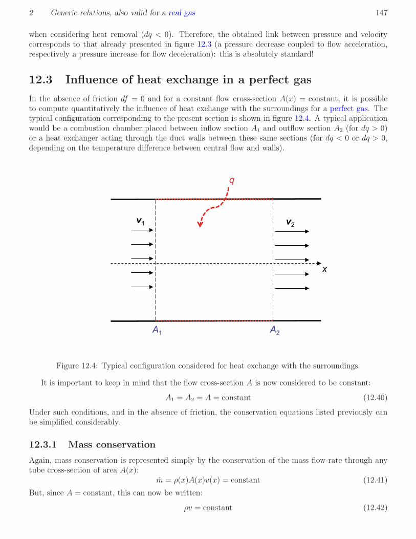
2 Generic relations, also valid for a real gas 147
when considering heat removal (dq < 0). Therefore, the obtained link between pressure and velocitycorresponds to that already presented in figure 12.3 (a pressure decrease coupled to flow acceleration,respectively a pressure increase for flow deceleration): this is absolutely standard!
12.3 Influence of heat exchange in a perfect gas
In the absence of friction df = 0 and for a constant flow cross-section A(x) = constant, it is possibleto compute quantitatively the influence of heat exchange with the surroundings for a perfect gas. Thetypical configuration corresponding to the present section is shown in figure 12.4. A typical applicationwould be a combustion chamber placed between inflow section A1 and outflow section A2 (for dq > 0)or a heat exchanger acting through the duct walls between these same sections (for dq < 0 or dq > 0,depending on the temperature difference between central flow and walls).
A1
x
v1
q
A2
v2
Figure 12.4: Typical configuration considered for heat exchange with the surroundings.
It is important to keep in mind that the flow cross-section A is now considered to be constant:
A1 = A2 = A = constant (12.40)
Under such conditions, and in the absence of friction, the conservation equations listed previously canbe simplified considerably.
12.3.1 Mass conservation
Again, mass conservation is represented simply by the conservation of the mass flow-rate through anytube cross-section of area A(x):
m = ρ(x)A(x)v(x) = constant (12.41)
But, since A = constant, this can now be written:
ρv = constant (12.42)

148 Chapter 12. Compressible flows with friction and heat exchange
Comparing the flow conditions when entering and leaving the domain of interest, it comes simply:
ρ1v1 = ρ2v2 (12.43)
12.3.2 Conservation of momentum
In the absence of friction, it comes first:
dp+ ρvdv = 0 (12.44)
But, again due to the fact that A = constant, it is now possible to obtain an integrated form of thisdifferential relation:
p+ ρv2 = constant (12.45)
This can be easily understood by differentiating again this relation, leading to:
dp+ v2dρ+ 2ρvdv = 0 (12.46)
Rewriting successively:
dp+ ρvdv + v2dρ+ ρvdv = 0
dp+ ρvdv + v (vdρ+ ρdv) = 0
dp+ ρvdv + d(ρv) = 0
(12.47)
The original result Eq.(12.44) is finally retrieved by using the mass conservation for a constant cross-section, Eq.(12.42), so that d(ρv) = 0. Finally, the integral formulation comparing flow momentumwhen entering and leaving the domain of interest reads:
p1 + ρ1v21 = p2 + ρ2v
22 (12.48)
12.3.3 Energy conservation
To close the system, it is enough to write now the conservation equation for energy. Taking into accountthe specific heat q (in J/kg) exchanged with the surroundings between inflow (A1) and outflow (A2), itreads:
h1 +v1
2
2+ q = h2 +
v22
2(12.49)
From the exchanged specific heat q, the associated heating power (in W) can be readily computed as:
P = mq (12.50)
Now, considering a perfect gas, Equation (B.16) reads:
h = cpT (12.51)
so that we can rewrite:
cpT1 +v1
2
2+ q = cpT2 +
v22
2(12.52)
or alternatively
cpT01 + q = cpT02 (12.53)
by introducing now the stagnation temperature T0. Remember that the stagnation temperature is aconserved quantity in an isentropic flow; however, the present flow is certainly not isentropic, sinceheat exchange is taking place with the surroundings. Therefore, the stagnation temperature T01 beforeheat exchange is not equal to T02 (after completion of heat exchange). Indeed, Eq.(12.53) shows thatT02 > T01 for q > 0, while T02 < T01 for q < 0.

2 Generic relations, also valid for a real gas 149
12.3.4 Solution procedure
Now, how is it possible to compute the outflow conditions (index 2) knowing the inflow conditions (index1) and the heat q exchanged between A1 and A2? The answer is quite simple when starting from thealternative formulation for the mass flow-rate introduced in Chapter 11, Eq.(11.79):
m = C p0A∗
(rT0)1/2
(12.54)
In the present case, this relation can be written before and after the region associated with heat exchange:
m1 = C p01A∗1
(rT01)1/2
m2 = C p02A∗2
(rT02)1/2
Please keep in mind that the quantities appearing on the right-hand side (p0, T0, A∗), while being constantin an isentropic flow, are now expected to change due to heat exchange and to the corresponding changein specific entropy s! This is true for the stagnation pressure p0 and stagnation temperature T0, butalso for the critical cross-section A∗. In the present configuration, the value of A∗1 or A∗2 is probablyonly a theoretical critical cross-section, with no real geometrical signification. Anyway:
p01 6= p02
T01 6= T02
A∗1 6= A∗2
To solve the problem, the energy conservation equation (12.53) is first inverted, knowing the initialconditions (and hence T01) and the exchanged heat q:
T02 = T01 +q
cp(12.55)
Using now the fact that the mass flow-rate is not modified by the heat release for such a steady internalflow (m1 = m2), Equation (12.54) can be used before and after heat exchange to obtain:
C p01A∗1
(rT01)1/2
= C p02A∗2
(rT02)1/2
(12.56)
Simplifying C and r leads to:p01A∗1
(T01)1/2
=p02A∗2
(T02)1/2
(12.57)
This can be rewritten as:(T02
T01
)1/2
=p02p01
A∗2
A∗1(12.58)
Now, it is enough to modify artificially the right-hand side as:
(T02
T01
)1/2
=
(
p1p01
p2p1
p02p2
)(A1
A∗1
A2
A1
A∗2
A2
)
(12.59)
Since the cross-section is constant, the term A2/A1 on the right-hand side is unity and disappears. Theratios p/p0 before (index 1) and after heat exchange (index 2) can be expressed by the function π(M)defined in Eq.(11.68) for isentropic compressible flows in Chapter 11:
π(M) = p/p0 (12.60)

150 Chapter 12. Compressible flows with friction and heat exchange
This relation is still valid in the present case, since it is only a relation between local flow conditions, andis therefore not impacted by global entropy variations between inflow section A1 and outflow section A2.For the same reason, the ratios A/A∗ appearing in Eq.(12.59) can be expressed by the function Σ(M)defined in Eq.(11.78) for isentropic compressible flows in Chapter 11:
Σ(M) =A
A∗
(12.61)
Therefore, Eq.(12.59) can be rewritten as:
(T02
T01
)1/2
=p2p1
π1
π2
Σ1
Σ2(12.62)
The pressure ratio, first term on the right-hand side, is the only one that still should be replaced in orderto obtain the final solution. For this purpose, the suitable starting point is the conservation equationfor momentum, Eq.(12.64). It can be rewritten successively:
p+ ρv2 = p
(
1 +ρv2
p
)
= p
(
1 +γρv2
γp
)
= p
(
1 + γv2
γp/ρ
)
= p
(
1 + γv2
c2
)
= p(
1 + γM2)
(12.63)
Hence, conservation of momentum can be rewritten for a configuration without friction and for a constantcross-section A as:
p(
1 + γM2)
= constant (12.64)
Applying this relation to both sides of Eq.(12.48), one obtains:
p1(
1 + γM21
)
= p2(
1 + γM22
)
(12.65)
Finally, the pressure ratio between inflow and outflow can be rewritten as:
p2p1
=1 + γM2
1
1 + γM22
(12.66)
Replacing in Eq.(12.62), one obtains the final solution:
T02
T01=
(
1 + γM21
1 + γM22
π1
π2
Σ1
Σ2
)2
(12.67)
All the terms appearing on the right-hand side of Eq.(12.67) can be directly computed or read fromthe Tables in Appendix E or Appendix F (provided that γ = 1.4), as long as the local Mach number isknown. Defining as new function:
Φ(M) :=(
1 + γM2)
π(M)Σ(M) (12.68)

2 Generic relations, also valid for a real gas 151
Equation (12.67) can be equivalently recast as:
T02
T01=
(
Φ(M1)
Φ(M2)
)2
(12.69)
Now, the solution procedure is clear:
• Knowing the starting conditions before heat exchange (index 1), compute Φ(M1) and T01;
• Using the energy conservation equation (12.55) and the heat exchanged q, deduce T02;
• Knowing now the ratio T02/T01 and Φ(M1), deduce Φ(M2) from Eq.(12.69);
• Invert to obtain M2 from Φ(M2);
• Knowing now the Mach number M2 after heat exchange, all other flow quantities can be directlydeduced! For instance, the pressure p2 is obtained from the Mach numbers and p1 using Eq.(12.66).The temperature T2 is obtained from T02 and M2 thanks to Eq.(11.62). And so on. . .
0.5 1 1.5 2 2.5 3 3.5 41.2
1.4
1.6
1.8
2
2.2
2.4
Mach number
Fun
ctio
n P
hi
Figure 12.5: Evolution of the function Φ with the Mach number M .
12.3.5 Flow modifications
As discussed in section 12.2.2, heat addition leads to the same flow modifications as a reduction incross-section A, while heat removal leads to the same flow modifications as an increase in cross-section

152 Chapter 12. Compressible flows with friction and heat exchange
Quantity For M1 < 1 For M1 > 1T0 ր րM ր1 ց1
v ր ցp ց րp0 ց ցT ? ր
Table 12.1: Evolution of the main flow quantities for heat addition (q > 0) without friction and for aconstant cross-section A, including limit values for the Mach number
A. Using this analogy and possibly computing all resulting quantities following the explanations of theprevious section, it is possible to summarize the corresponding impact for heat addition (q > 0), thisbeing probably the most usual application (Table 12.1).
The question mark appearing for the temperature T when starting from subsonic conditions mightbe surprising. Indeed, it is possible to “cool down” a compressible flow by heat addition! To understandthis point, let us start again from the mass flow-rate:
m = ρAv (12.70)
The density might be replaced by p/(rT ) using the ideal gas law, Eq.(B.8). From the definition of theMach number, Eq.(11.29), it is easy to replace v by (Mc) = (M
√γrT ). Finally, it comes in this manner:
m =(√
γ
rA)pM√T
(12.71)
Since all terms in the first parenthesis (γ, r, A) are here constant, and since the mass flow-rate is alsoconstant, it ensues that the last ratio on the right hand-side must be constant as well:
pM√T
= constant (12.72)
Using logarithmic differentiation, one obtains:
dp
p+
dM
M− 1
2
dT
T= 0 (12.73)
Or alternatively:dT
T= 2
dp
p+ 2
dM
M(12.74)
Using again logarithmic differentiation starting from Eq.(12.64), one obtains now:
dp
p+
2γM dM
1 + γM2= 0 (12.75)
Combining the last two relations to eliminate dp/p leads to:
dT
T= 2
dM
M− 4γM dM
1 + γM2
=2dM
M (1 + γM2)
(
1 + γM2 − 2γM2)

2 Generic relations, also valid for a real gas 153
Finally:dT
T=
2dM
M
1− γM2
1 + γM2(12.76)
This explains the question mark in Table 12.1. Indeed, heat addition (q > 0) in a subsonic flow (M1 < 1,so that dM > 0) leads to a temperature increase (dT > 0) as long as M1 < 1/
√γ, which is probably
intuitive. However, the same heat addition just before reaching sonic conditions (for 1/√γ ≤ M1 ≤ 1)
now leads to cooling: T2 < T1! Physically, this is due to the fact that both contributions in the energyconservation equation (12.52), interact with each other. While it is directly clear that T0, a measure forthe total energy, will increase in case of heat addition (Eq. 12.53), this is not necessarily so for T , whichis only a measure of the internal energy of the fluid.
12.3.6 Thermal choking
Let us close this section by a last but important qualitative remark. Looking again at Eq.(12.69), it isclear that heat addition (q > 0) will always lead to a decrease of the function Φ(M) i.e., Φ(M2) < Φ(M1),since T02 > T01. Looking now at figure 12.5, this condition implies - as expected from the qualitativeprocess described in section 12.2.2, also documented in Table 12.1 - that the Mach number will increase(M2 > M1) due to heat addition in a subsonic flow, while it will decrease (M2 < M1) for heat additionin a supersonic flow.
Now, Figure 12.5 clearly shows that the function Φ(M) reaches a minimum for M = 1. At thatpoint, it is impossible to find any flow evolution allowing a further decrease of Φ. This is the explanationfor the problem called thermal choking. This process corresponds to excessive heat addition, usually ina subsonic flow. Under such conditions, the Mach number will progressively increase. If more heat isadded, it will increase further, and so on. But, when reaching the limit value M = 1, it is absolutelyimpossible to add more heat into this flow. When nevertheless attempting to do so, the flow willabruptly react by. . . stopping completely! Remember that heat addition is qualitatively similar to areduction of the flow cross-section, A. Thermal choking corresponds in this analogy to a duct beingcompletely closed. Clearly, thermal choking will have extremely severe consequences (flame extinctiondue to interruption of the air flow, very large forces acting suddenly on the system. . . ) and must beavoided by all means. In modern systems, the electronic regulation will prevent the user from addingadditional heat when coming too close to the sonic conditions.
12.4 Influence of friction
After this extensive analysis of heat exchange, let us now consider the alternative process, associated tofriction. In the absence of heat exchange (dq = 0) and for a constant flow cross-section (A(x) = A =constant), it is indeed possible to compute quantitatively the influence of friction. We will neverthelessstart with a qualitative analysis. The typical configuration corresponding to the present section is shownin figure 12.6. Typical applications involve pressurized gas lines with a noticeable length, l ≫ 1 m.
For a qualitative analysis, the generalized Hugoniot equation (12.32) can now be simplified by takinginto account the hypotheses listed above as:
(
1−M2) dv
v=
1
ρc2
(
1 +k2
ρT
)
dffx (12.77)
This equation reveals, that in the absence of friction (dffx = 0), the flow velocity will remain constant(dv = 0), as expected for such conditions (no change of flow cross-section, no heat exchange, no friction).Introducing now the impact of friction in the analysis (hence dffx > 0), a subsonic condition (M1 < 1 atthe beginning of the analysis, and hence (1−M2
1 ) > 0) leads to dv > 0. In other words, taking friction

154 Chapter 12. Compressible flows with friction and heat exchange
A1
x
v1
A2
v2
Friction force dFf
Figure 12.6: Typical configuration considered when taking into account friction.
into account in a subsonic flow leads to flow acceleration, which appears to be clearly counter-intuitive:systems with friction are usually slower, not faster, than comparable friction-free conditions!
Let us explain this apparent contradiction. For this purpose, the conservation equations will be firstspecified for the conditions considered presently.
12.4.1 Mass conservation
As discussed previously when considering heat exchange, mass conservation (m = constant) for a con-stant flow cross-section A = constant simply corresponds to
ρv = constant (12.78)
The logarithmic differential form of this relation will be even more useful:
dρ
ρ+
dv
v= 0 (12.79)
Comparing the flow conditions when entering and leaving the domain of interest, it comes simply:
ρ1v1 = ρ2v2 (12.80)
12.4.2 Conservation of momentum
The general equation (12.12) derived at the beginning of this chapter stays unchanged.
dp+ ρvdv + dffx = 0 (12.81)

2 Generic relations, also valid for a real gas 155
12.4.3 Energy conservation
Here, the solution for q = 0 simply reads:
h+v2
2= constant (12.82)
In differential form, one obtains:dh+ vdv = 0 (12.83)
Comparing again the flow conditions when entering and leaving the domain of interest, it comes simply:
h1 +v1
2
2= h2 +
v22
2(12.84)
12.4.4 Qualitative analysis
Starting from Eq.(12.39), it is now possible to suppress the contribution of heat, since dq = 0. It comes:
dp =dffx
M2 − 1
(
1 +k2M2
ρT
)
(12.85)
From this relation, it is clear that the observed acceleration (dv > 0) for a subsonic flow (M < 1)involving friction (dffx > 0) is indeed simply a consequence of pressure loss, dp < 0, and thereforenothing surprising. In the same manner, a supersonic flow (M > 1) with friction (dffx > 0) will leadto a deceleration (dv < 0) coupled to a pressure increase (dp > 0). Such combinations are absolutelystandard: we have found exactly the same for incompressible flows when analyzing the Bernoulli equationin Chapter 6!
12.4.5 Quantitative solution procedure
Pursuing now the aim of a quantitative analysis, the conversation equation for momentum (Eq. 12.12)divided by the density is a perfect starting point:
dp
ρ+ vdv +
dffxρ
= 0 (12.86)
The last term on the left-hand side describes the friction loss. A suitable description for this friction losshas been already presented in Chapter 6 (see Eq.6.38 when deriving the generalized Bernoulli equation:the law of Darcy-Weisbach):
dffxρ
= def
= fdx
d
v2
2(12.87)
In this equation, the only difference with the original Eq.(6.38) is the differential flow length dx appearinginstead of the integral flow length l, since the present equation is in differential form. Using now thismodel, the conservation equation for momentum reads:
dp
ρ+ vdv + f
dx
d
v2
2= 0 (12.88)
with f the friction factor.

156 Chapter 12. Compressible flows with friction and heat exchange
A logarithmic differentiation of the ideal gas law, Eq.(B.8), leads to:
dp
p=
dρ
ρ+
dT
T(12.89)
since r = constant. Hence:
dp = pdρ
ρ+
p
TdT (12.90)
Since, from Eq.(12.79):dρ
ρ= −dv
v(12.91)
it comes:
dp = −pdv
v+
p
TdT (12.92)
Hence:dp
ρ= −p
ρ
dv
v+
p
ρTdT (12.93)
Using again twice the ideal gas law, Eq.(B.8), one obtains finally for the right-hand side:
dp
ρ= −rT
dv
v+ rdT (12.94)
This relation is now used to replace the first term in Eq.(12.88), leading to:
− rTdv
v+ rdT + vdv + f
dx
d
v2
2= 0 (12.95)
or equivalently:(
v2 − rT) dv
v+ rdT + f
dx
d
v2
2= 0 (12.96)
Now, the energy equation (12.83) can be transformed for a perfect gas into:
vdv = −dh
= −cpdT
(12.97)
It is then possible to write successively, using Eq.(B.6):
dT = − v
cpdv
rdT = − r
cpvdv
= − rγrγ−1
vdv
= −γ − 1
γvdv
= −γ − 1
γv2
dv
v(12.98)
This relation is now used to replace the second term in Eq.(12.96), leading to:
(
v2 − rT) dv
v− γ − 1
γv2
dv
v+ f
dx
d
v2
2= 0 (12.99)

2 Generic relations, also valid for a real gas 157
By combining the first two terms, one obtains:
(
v2
γ− rT
)
dv
v+ f
dx
d
v2
2= 0 (12.100)
Now, let us introduce again the critical Mach number:
M∗ =v
c∗(12.101)
Inverting this relation:
v = c∗M∗ (12.102)
Since the present flow is adiabatic, the stagnation temperature T0 and as a consequence the criticalspeed of sound c∗ are constant (see again Eq.11.37). A logarithmic differentiation of Eq.(12.102) leadstherefore to:
dv
v=
dM∗
M∗
(12.103)
It is now useful to introduce simultaneously Eqs.(12.102) and (12.103) into Eq.(12.100) in order toreplace everywhere the flow velocity v (respectively the ratio dv/v):
(
c2∗M2∗
γ− rT
)
dM∗
M∗
+ fdx
d
c2∗M2∗
2= 0 (12.104)
Multiplying now this relation by γ/c2∗, it comes:
(
M2∗ − γrT
c2∗
)
dM∗
M∗
+ fdx
d
γM2∗
2= 0 (12.105)
Considering Eq.(11.37):
c∗ =
√
2γ
γ + 1rT0 (12.106)
the second term in the parenthesis of Eq.(12.105) reads:
γrT
c2∗= γrT
γ + 1
2γrT0
=γ + 1
2
T
T0(12.107)
It is then possible to rewrite Eq.(12.105):
(
M2∗ − γ + 1
2
T
T0
)dM∗
M∗
+ fdx
d
γM2∗
2= 0 (12.108)
Reminding now Eq.(11.92):T
T0
= 1− γ − 1
γ + 1M∗
2 (12.109)
Equation (12.108) can be modified into:
(
M2∗ − γ + 1
2+
γ + 1
2
γ − 1
γ + 1M∗
2
)
dM∗
M∗
+ fdx
d
γM2∗
2= 0 (12.110)

158 Chapter 12. Compressible flows with friction and heat exchange
which simplifies successively into:(γ + 1
2M∗
2 − γ + 1
2
)dM∗
M∗
+ fdx
d
γM2∗
2= 0
γ + 1
2
(
M∗2 − 1
) dM∗
M∗
+ fdx
d
γM2∗
2= 0 (12.111)
Dividing finally byγ + 1
2M2
∗ :(
M∗2 − 1
) dM∗
M3∗
+ fγ
γ + 1
dx
d= 0 (12.112)
In preparation for integration between inflow cross-section (index 1) and outflow cross-section (index 2),this relation is expanded into:
dM∗
M∗
− dM∗
M3∗
+
[
γ
γ + 1
f
d
]
dx = 0 (12.113)
Noticing that the last term between square brackets is constant, integration in space leads to:∫ 2
1
dM∗
M∗
−∫ 2
1
dM∗
M3∗
+
[
γ
γ + 1
f
d
]∫ 2
1dx = constant (12.114)
The integration of all three terms on the left-hand side is straightforward and leads to:
[lnM∗]21 +
[
1
2
1
M2∗
]2
1
+γ
γ + 1fl
d= constant (12.115)
introducing in the last term l := x2 − x1, the total length of the system between inflow cross-section(index 1) and outflow cross-section (index 2). One therefore obtains:
lnM∗2 − lnM∗1 +1
2
(
1
M2∗2
− 1
M2∗1
)
+γ
γ + 1fl
d= constant (12.116)
When considering an infinitely short tube (so that l → 0), one would obviously obtain as well M∗2 → M∗1
and the left-hand side of this equation would naturally vanish. Therefore, the only possible value for theconstant appearing on the right-hand side is 0. The final solution allowing to compute the influence offriction in a compressible flow without heat exchange and for a constant cross-section therefore reads:
ln(M∗2
M∗1
)
+1
2
(
1
M2∗2
− 1
M2∗1
)
+γ
γ + 1fl
d= 0 (12.117)
12.4.6 Flow modifications
As discussed in section 12.2.2, friction leads qualitatively to the same flow modifications as a reductionin cross-section A. However, the flow remains adiabatic. Using this analogy and possibly computingall resulting quantities following the explanations of the previous section, it is possible to summarizethe corresponding impact of friction (dffx > 0), this being the most usual application (Table 12.2).Considering that there is again an extremal value for sonic conditions, flow choking can be obtained asa consequence of friction, similarly to the thermal choking discussed previously.
12.5 Conclusions
Now, one-dimensional compressible flows can be solved accurately even with friction or heat exchange.Such flows, when in the supersonic regime, will be often strongly modified due to the occurrence ofshock waves: this will be the subject of the next chapter.

2 Generic relations, also valid for a real gas 159
Quantity For M1 < 1 For M1 > 1T0 = =M ր1 ց1
v ր ցp ց րp0 ց ցT ց ր
Table 12.2: Evolution of the main flow quantities for friction without heat exchange and for a constantcross-section A, including limit values for the Mach number

160 Chapter 12. Compressible flows with friction and heat exchange

Chapter 13
Shock waves
13.1 Introduction
In many practical supersonic flows, discontinuities are observed. This means that the parameters de-scribing the flow will vary strongly and over very short distances, typically of the order of magnitudeof the mean free path. Under such conditions, the hypotheses underlying the continuum assumptiondiscussed in Section 1.3 are not valid any more. It is thus impossible to use the conservation equationsdeveloped previously to investigate the inner structure of such discontinuities. However, it is still possi-ble to relate the flow conditions encountered in front of and behind such discontinuities, as will be donein what follows. This is in practice sufficient to solve most relevant problems. If the solution withinthe discontinuity is of interest, a specific description based on Statistical Physics must be used for thispurpose.
Figure 13.1: Example of shock waves in practical flows: attached to a plane breaking the sound barrier(left, photo from RC Clubs); behind an engine of the Space Shuttle at start (center, photo from NASA);when firing a bullet (right, photo from Subtopia).
The only discontinuities we will consider in this document are shock waves (Figure 13.1). Twodifferent kinds of shock waves will be solved for. In a first step, the normal shock wave, perpendicularto the main flow direction, will be described in detail. The obtained results will then be extendedtowards the oblique shock wave, inclined towards the main flow direction. Note that only straight shockwaves will be accepted. In practice, curved shock waves can also be found, but this is a less relevantconfiguration that can hardly be solved by analytical means.
161

162 Chapter 13. Shock waves
13.2 Normal shock wave
13.2.1 Considered configuration and hypotheses
The generic configuration considered for the analysis of a normal shock wave is depicted in figure 13.2.
v1 v2
p1
1
T1
p2
2
T2
Figure 13.2: Configuration employed for the analysis of a fixed, normal shock wave (shown in red),together with the control volume (in green) used to derive the conservation equations.
The hypotheses underlying the analysis are as follows, and correspond indeed quite well to thephysical reality:
• The shock wave is a discontinuity without inner structure, separating the upstream flow (withconditions marked by an index 1) from the downstream flow (with conditions marked by an index2);
• The shock wave is a straight structure, normal to the flow direction; hence, all streamlines areparallel to each other and perpendicular (or normal) to the shock wave;
• The configuration is steady.
13.2.2 Conservation equations for a real gas
We begin by considering generic gas properties. This means that the relations derived in this section arevalid even for complex thermodynamic relations, as might be found for a real gas. Taking into accountthe hypotheses listed above, it is possible to establish generic conservation equations.

2 Normal shock wave 163
Mass conservation
For the steady flow bounded by the streamtube shown in green in figure 13.2 the mass conservationis represented simply by the conservation of the mass flow-rate through any tube cross-section of areaA(x):
m = ρ(x)A(x)v(x) = constant (13.1)
Here, all streamlines are parallel to each other and horizontal, so that the cross-section of the streamtubeis constant, A(x) = A1 = A2 = constant.
Hence, the mass conservation relating upstream and downstream conditions simply reads:
ρ1v1 = ρ2v2 (13.2)
Conservation of momentum
The developments in this section follow closely those presented when considering heat exchange in acompressible flow, see Section 12.3.2.
Friction plays obviously no role for the configuration considered in figure 13.2, since there is novelocity gradient upstream and downstream of the discontinuity (homogeneous flow conditions). In theabsence of friction, conservation of momentum in a compressible flow reads as usual in differential form(see also Eqs. (11.16) and (12.44)):
dp+ ρvdv = 0 (13.3)
But, again due to the fact that A = constant, it is now possible to obtain an integrated form of thisdifferential relation, as demonstrated in Section 12.3.2:
p+ ρv2 = constant (13.4)
Finally, conservation of momentum through the normal shock wave simply reads:
p1 + ρ1v21 = p2 + ρ2v
22 (13.5)
Energy conservation
The conservation of energy is again simply derived from the First Law of Thermodynamics. For such anisolated adiabatic system, the total energy is constant, which can be written when neglecting as usualthe contribution of potential energy for this gaseous flow:
h1 +v212
= h2 +v222
(13.6)
13.2.3 Conservation equations for a perfect gas
The previous relations are only slightly modified when considering the special case of a perfect gas, asdone in the rest of this section. Using Eq.(11.42), one obtains for:
• Mass conservation (unchanged):
ρ1v1 = ρ2v2 (13.7)
• Conservation of momentum (unchanged):
p1 + ρ1v21 = p2 + ρ2v
22 (13.8)

164 Chapter 13. Shock waves
• Energy conservation:
cpT1 +v212
= cpT2 +v222
(13.9)
which might also be rewritten using the stagnation temperature T0 that takes into account boththe internal energy and the kinetic energy of the fluid:
cpT01 = cpT02 (13.10)
Since cp = constant, it is thus again clear that, in this adiabatic flow, the stagnation temperature T0
is the same upstream and downstream of the shock wave. This simple observation will be veryuseful to solve the problem:
T01 = T02 (13.11)
13.2.4 Jump relations involving M1 and M2
Using Eq.(11.62) to relate temperature T to stagnation temperature T0, once upstream of the shock(link between T1 and T01) and once downstream of the shock (link between T2 and T02), it comes:
T01
T1= 1 +
γ − 1
2M2
1 (13.12)
T02
T2= 1 +
γ − 1
2M2
2 (13.13)
Dividing now the first equation by the second one and keeping in mind that T01 = T02, one obtainssimply the relation quantifying the temperature jump through the normal shock:
T2
T1=
1 + γ−12M2
1
1 + γ−12M2
2
(13.14)
Reminding now Eq.(12.64), an alternative form of the conservation of momentum (Eq. 13.5) in theabsence of friction and for a constant cross-section A, both hypotheses being valid as well in the presentcase, it is possible to relate upstream and downstream conditions by:
p1(
1 + γM21
)
= p2(
1 + γM22
)
(13.15)
Hence, the relation quantifying the pressure jump through the normal shock is simply:
p2p1
=1 + γM2
1
1 + γM22
(13.16)
Using now the ideal gas relation (Eq. 11.38), one obtains directly for the density jump through thenormal shock:
ρ2ρ1
=p2rT2p1rT1
=p2p1
T1
T2(13.17)
which is sufficient knowing Eqs.(13.14) and (13.16).

2 Normal shock wave 165
13.2.5 Relation between the Mach numbers upstream and downstream ofthe normal shock
The relations written in the previous section still involve both Mach numbers M1 (before the normalshock) and M2 (after the normal shock). However, in most cases, only the conditions upstream of theshock are known. To close the problem, it is therefore necessary to solve for M2 knowing the condi-tions before the normal shock (index 1). For this purpose, we start again from the mass conservation,Eq.(13.2):
ρ1v1 = ρ2v2 (13.18)
We then rewrite, using the obvious relation v = Mc:
ρ2ρ1
=v1v2
=M1c1M2c2
(13.19)
On the left-hand side, the density jump is replaced using Eq.(13.17). On the right-hand side, thespeed of sound c is replaced using Eq.(11.51), obtaining finally:
p2p1
T1
T2=
M1
√γrT1
M2
√γrT2
(13.20)
Simplifying γ and r and lumping together the temperature jumps on the left and right side of theequation, it comes:
p2p1
=M1
M2
√
T2
T1
(13.21)
Replacing the pressure jump and temperature jump appearing in this equation using Eqs.(13.16) and(13.14), one obtains finally:
1 + γM21
1 + γM22
=M1
M2
√√√√1 + γ−1
2M2
1
1 + γ−12M2
2
(13.22)
Taking the whole equation to the square and rewriting it using M1 as a known value and M2 as theunknown, one recognizes finally a simple quadratic polynomial equation involving M2
2 as unknown value,in the form:
aM42 + bM2
2 + c = 0 (13.23)
It is easy to show that this equation delivers two possible solutions for M22 and, reminding that both
M1 and M2 must be positive values, the two solutions correspond simply to:
1. The case with no shock at all, M2 = M1! Reporting in all jump relations derived in the previoussection, this leads of course to T2 = T1, p2 = p1, ρ2 = ρ1. . . This should not be a surprise: the shockwave represented in figure 13.2 cannot be forced to be there. In other words, the case withouta shock wave is also a physically possible solution. In that case, the flow remains obviouslyunchanged. We will not consider further this case in the rest of this chapter.
2. The really interesting case, i.e., that with a normal shock wave, corresponds to the second solutionof the quadratic equation, which reads:
M2 =
√√√√2 + (γ − 1)M2
1
2γM21 + 1− γ
(13.24)

166 Chapter 13. Shock waves
Figure 13.3 shows the relation between M1 and M2 for a supersonic upstream condition (M1 ≥ 1),since this is the only relevant case, as will be shown later. In this figure, it is clearly observed that, forM1 ≥ 1, one obtains M2 ≤ 1, so that the normal shock wave separates a supersonic region (upstream)from a subsonic region (downstream of the normal shock). When increasing M1, the value of M2,the Mach number downstream of the normal shock, decreases monotonically. Additionally, as directlyvisible from Eq.(13.24), there is a minimum value for M2 at very high incoming Mach number M1:
M2 lim = limM1→∞
M2 =
√
γ − 1
2γ(13.25)
For γ = 1.4, this minimum value corresponds to M2 lim = 0.378.
1 2 3 4 50.4
0.5
0.6
0.7
0.8
0.9
1
Mach number in front of shock wave M 1
Mac
h nu
mbe
r M
2 beh
ind
shoc
k
Figure 13.3: Relation between the Mach numbers upstream and downstream of the normal shock.
13.2.6 Jump relations involving only the upstream Mach number M1
Using now Eq.(13.24) in order to eliminate the value of M2 in all the jump relations presented in Section13.2.4 and simplifying the obtained equation, it is slightly tedious but very straightforward to obtain allthe jump relations as a direct function of the Mach number M1 upstream of the normal shock only. It

2 Normal shock wave 167
comes successively, first combining Eq.(13.24) and Eq.(13.16):
p2p1
=2γM2
1 − γ + 1
γ + 1(13.26)
The corresponding evolution of the pressure jump is shown in figure 13.4 as a function of the upstreamMach number M1 for M1 ≥ 1. Very large values are found for p2/p1 when increasing M1, showing thata normal shock wave typically leads to a very strong increase in pressure. The value of p2 tends towardinfinity when M1 → ∞. This, together with the strong deceleration discussed previously in connectionwith figure 13.3 and quantified by Eq.(13.24), is typically the most noticeable effect of a normal shockwave. Obviously, it can also be a very dangerous effect if this shock wave is associated to an explosion,as discussed later!
1 2 3 4 50
5
10
15
20
25
30
Mach number in front of shock wave M 1
Pre
ssur
e ju
mp
p 2/p1
Figure 13.4: Pressure jump through the normal shock wave as a function of the upstream Mach numberM1. The dashed blue line denotes the level p2/p1 = 1.
Combining now Eq.(13.24) and Eq.(13.14), it comes:
T2
T1=
(
2γ
γ + 1M2
1 − γ − 1
γ + 1
)(
γ − 1
γ + 1+
2
(γ + 1)M21
)
(13.27)
The corresponding evolution of the temperature jump is shown in figure 13.5 as a function of theupstream Mach number M1 for M1 ≥ 1. Relatively large values are found for T2/T1 when increasing

168 Chapter 13. Shock waves
M1, showing that a normal shock wave typically leads to a large increase in temperature. The value ofT2 tends toward infinity when M1 → ∞.
1 2 3 4 51
2
3
4
5
6
Mach number in front of shock wave M 1
Tem
pera
ture
jum
p T 2/T
1
Figure 13.5: Temperature jump through the normal shock wave as a function of the upstreamMach number M1.
Following Eq.(13.17), it is now sufficient to divide Eq.(13.26) by Eq.(13.27) to obtain the densityjump, leading to:
ρ2ρ1
=(γ + 1)M2
1
2 + (γ − 1)M21
(13.28)
The corresponding evolution of the density jump is shown in figure 13.6 as a function of the upstreamMach number M1 for M1 ≥ 1. Relatively large values are found for ρ2/ρ1 when increasing M1, showingthat a normal shock wave typically leads to a large increase in density.
Using mass conservation, Eq.(13.2), it follows immediately that:
v1v2
=ρ2ρ1
(13.29)
so that the velocity jump is given by:
v2v1
=2 + (γ − 1)M2
1
(γ + 1)M21
(13.30)

2 Normal shock wave 169
1 2 3 4 51
2
3
4
5
6
Mach number in front of shock wave M 1
De
nsity ju
mp
ρ2
/ρ1
Figure 13.6: Density jump through the normal shock wave as a function of the upstream Mach numberM1.
The obtained curve illustrating the deceleration observed in a normal shock wave (v2 ≤ v1) behaves inopposite manner to that shown in figure 13.6, and is shown in figure 13.7.
Looking at the last two equations, it is also obvious that density and velocity jump converge to alimit value when increasing M1:
limM1→∞
ρ2ρ1
= limM1→∞
v1v2
=γ + 1
γ − 1(13.31)
For γ = 1.4, one obtains therefore limM1→∞ρ2ρ1
= 6 and limM1→∞v2v1
= 1/6 = 0.1667.The change in stagnation pressure through the normal shock wave can be directly computed by
writing:p02p01
=p02p2
p2p1
p1p01
(13.32)
On the right-hand side of this equation, the first and third ratios correspond to the local relation betweenpressure and stagnation pressure, discussed extensively in Chapter 11 and defined by Eq.(11.67) as theinverse of function π, see Eq.(11.68). The second ratio on the right-hand side of the previous equationis the pressure jump through the normal shock wave, already given by Eq.(13.26). Hence, it comes:
p02p01
=
[(
1 +γ − 1
2M2
2
) γ
γ−1
]
2γM21 − γ + 1
γ + 1
[(
1 +γ − 1
2M2
1
)−γ
γ−1
]
(13.33)

170 Chapter 13. Shock waves
1 2 3 4 50
0.2
0.4
0.6
0.8
1
Mach number in front of shock wave M 1
Vel
ocity
jum
p v 2/v
1
Figure 13.7: Velocity jump through the normal shock wave as a function of the upstream Mach numberM1.
This can be first rewritten as:
p02p01
=
(
1 + γ−12M2
1
1 + γ−12M2
2
)γ (γ + 1
2γM21 − γ + 1
)γ−1
−1
γ−1
(13.34)
Recognizing now in the first parenthesis the temperature jump T2/T1, see Eq.(13.14), it is possible toreformulate this parenthesis using Eq.(13.27). Simplifying all similar terms with each other, one obtainsfinally:
p02p01
=
[(
2γ
γ + 1M2
1 − γ − 1
γ + 1
)(
γ − 1
γ + 1+
2
(γ + 1)M21
)γ]− 1γ−1
(13.35)
The corresponding evolution of the jump in stagnation pressure through the normal shock wave is shownin figure 13.8 as a function of the upstream Mach number M1 for M1 ≥ 1. The stagnation pressure islower behind the shock, showing that the normal shock is a dissipative structure.
Now, one last question remains: why have we decided to plot figures 13.4 to 13.8 only for a supersonicupstream condition, M1 ≥ 1? This will be justified in the next section.

2 Normal shock wave 171
1 2 3 4 50
0.2
0.4
0.6
0.8
1
Mach number in front of shock wave M 1
Jum
p of
tota
l pre
ssur
e p 02
/p01
Figure 13.8: Jump in stagnation pressure through the normal shock wave as a function of the upstreamMach number M1.
13.2.7 Necessary condition on M1 for the existence of a shock
As a last relation between upstream and downstream conditions, it is very interesting to look at thespecific entropy of a perfect gas, given by Eq.(13.36):
s = cv ln
(
p
ργ
)
+ constant (13.36)
One therefore obtains immediately:
s2 − s1cv
= ln
(
p2p1
[
ρ1ρ2
]γ)
(13.37)
Replacing the pressure jump using Eq.(13.26) and the density jump using Eq.(13.28), one obtains:
s2 − s1cv
= ln
(
2γM21 − γ + 1
γ + 1
)(
(γ + 1)M21
2 + (γ − 1)M21
)γ
(13.38)
The corresponding evolution of the change in specific entropy through the normal shock wave isshown in figure 13.9 as a function of the upstream Mach number M1. For the first time, the full range

172 Chapter 13. Shock waves
of values for M1 is considered, also for subsonic upstream conditions! As can be seen, cases withM1 > 1 correspond to an increase in entropy, s2 > s1, which is fully OK. However, cases with a subsonicupstream condition, M1 < 1 would lead to a decrease in entropy, which would directly violate theSecond Law of Thermodynamics for the isolated system we are considering. Therefore, it is absolutelyimpossible to observe a steady normal shock wave in a subsonic flow. This explains why we have onlyconsidered the range M ≥ 1 for all figures 13.4 to 13.8: this is the only valid range for a fixed, steadynormal shock!
0 1 2 3 4 5−2
−1
0
1
2
Mach number in front of shock wave M 1
Ent
ropy
diff
eren
ce (
s 2−s 1)/
c v
Figure 13.9: Change in specific entropy through a normal shock wave as a function of the upstreamMach number M1.
Beware! This does not mean that a shock cannot exist in a subsonic flow, or even under quiescentconditions! But, in that case, the shock cannot remain steady and must propagate, so that the upstreamvelocity relative to the propagating shock is indeed in the supersonic range. This issue will be discussedlater in Section 13.2.14.
13.2.8 Shock relation of Prandtl
We start by recalling that the stagnation temperature is the same upstream and downstream of theshock wave, T01 = T02. Now, considering Eq.(11.37) demonstrated in Section 11.2.4, it is clear thatthe critical speed of sound is also unchanged when crossing the normal shock wave, c∗2 = c∗1. As a

2 Normal shock wave 173
Quantity EvolutionT0 T01 = T02
M (from M1 ≥ 1) ց (M2 ≤ 1)M∗ (M∗1 ≥ 1) ց [M∗2 = (1/M∗1)] ≤ 1v v1 ց v2p p1 ր p2p0 p01 ց p02T T1 ր T2
s s1 ր s2
Table 13.1: Evolution of the main flow quantities through a normal shock wave
consequence, it is possible to write using the critical Mach number defined in Eq.(11.34):
v2v1
=v2/c∗2v1/c∗1
=M∗2
M∗1
(13.39)
At the same time, comparing Eq.(13.30) with Eq.(11.90) demonstrated at the end of Chapter 11, it isimmediately clear that
v2v1
=1
M2∗1
(13.40)
Hence, it comes by equating the last two relations:
1
M2∗1
=M∗2
M∗1(13.41)
leading directly to the useful shock relation of Prandtl for normal shock waves:
M∗1M∗2 = 1 (13.42)
13.2.9 Summary: evolution of all quantities through a normal shock
All observations described in the previous sections are summarized in Table 13.1.
13.2.10 Normal shock tables
In order to facilitate later computations, the most important relations have been computed and theresults are tabulated in Appendix F (Appendix E is obviously not relevant, since a normal shock wavecan only exist for the upstream condition M1 ≥ 1. . . ). Remember that all values listed in Appendix Fare only valid for γ = 1.4. If this condition does not hold, it is necessary to use the equations listedpreviously in this chapter. Now, for γ = 1.4, and considering in the first column of this Table M = M1,the Mach number upstream of the steady normal shock wave:
• the eighth column gives the Mach number downstream of the shock wave, M2, following Eq.(13.24);
• the ninth column gives the pressure jump, Eq.(13.26);
• the tenth column gives the density jump, Eq.(13.28);
• the eleventh column gives the temperature jump, Eq.(13.27);
• the twelfth column gives the jump in stagnation pressure, Eq.(13.35).

174 Chapter 13. Shock waves
13.2.11 Solution and graphical representation using the critical Mach number
Since there is a direct connection between the Mach number and the critical Mach number (Eqs. 11.90and 11.91), as shown in Section 11.3.9 (see Chapter 11 for further details), all the relations establishedpreviously as function of the Mach number can be simply rewritten as function of the critical Mach number.
The shock relation of Prandtl (Eq. 13.42) can also be used for this purpose. Finally, one obtains analternative set of solution equations describing pressure jump, temperature jump, density jump. . . , asfunction of the critical Mach number M∗1 upstream of the normal shock.
Since a graphical representation cannot be overloaded, only the pressure jump and the jump ofstagnation pressure have been represented as function of critical Mach number M∗ (meaning here M∗1)in figure 11.8.
13.2.12 Relation of Rankine-Hugoniot
It is sometimes useful to analyze a normal shock wave without direct reference to the Mach numbers.For this purpose, the Rankine-Hugoniot relation makes a direct connection between the pressure jumpp2/p1 and the inverse of the density jump ρ1/ρ2 (which happens to be equal to the velocity jump v2/v1due to mass conservation, as discussed previously). In order to derive this relation, we start back fromEq.(13.26):
p2p1
=2γM2
1 − γ + 1
γ + 1(13.43)
We first invert this relation to obtain the upstream Mach number M1 as a function of the pressures p1and p2, leading to:
M21 =
(γ + 1)p2 + (γ − 1)p12γp1
(13.44)
This relation is used to replace M21 in the density jump, Eq.(13.28):
ρ2ρ1
=(γ + 1)M2
1
2 + (γ − 1)M21
(13.45)
After simplification, one obtains a relation where M1 does not appear any more:
ρ2ρ1
=(γ + 1)p2
p1+ γ − 1
(γ − 1)p2p1
+ γ + 1(13.46)
We finally invert this relation to obtain the pressure jump p2/p1 as function of ρ1/ρ2. This delivers theRankine-Hugoniot relation, valid for any normal shock wave:
p2p1
=
γ + 1
γ − 1− ρ1
ρ2γ + 1
γ − 1
ρ1ρ2
− 1(13.47)
The corresponding relation is displayed graphically as a red curve in figure 13.10. It is an hyperboliccurve. Any normal shock (for γ = 1.4) will correspond to a single point along this red curve.
The evolution corresponding to an isentropic process is shown as a black dashed line in the samefigure. Obviously, while the Rankine-Hugoniot relation only exists for p2 ≥ p1 and ρ2 ≥ ρ1 (as found in anormal shock), the isentropic evolution covers the whole set of density ratio ρ1/ρ2, since it can describe acompression as well as an expansion process. Confirming the results presented in figure 13.9, it appears

2 Normal shock wave 175
0 0.5 1 1.50
5
10
15
20
25
30
inverse density ratio ρ1/ρ
2
pre
ssu
re r
atio
p2/p
1
Rankine−Hugoniot relation
Isentropic relationRayleigh line (M
1=4)
Figure 13.10: Relation of Rankine-Hugoniot for γ = 1.4, valid for any normal shock (red line), comparedwith an Isentropic evolution (dashed black line). Additionally, the Rayleigh line for a specific shock (here,M1 = 4) is shown as a straight blue line.
again that a weak shock (i.e., a shock for M1 ≃ 1, or in other words p2 ≃ p1 is nearly isentropic: the redand black curves in 13.10 cannot be distinguished in this region, left of the point (1,1).
However, this is not true any more for a strong shock (M1 ≫ 1, or p2 ≫ p1)! In this part of thediagram, the two curves lie far from each other, and the pressure increase is much more considerable inthe normal shock for the same density variation.
13.2.13 Rayleigh line
As explained in the previous section, the Rankine-Hugoniot relation is valid for all normal shock waves.An additional condition is needed to obtain the conditions found in a specific shock, for a given valueof M1. For this purpose, the Rayleigh line will be plotted in the same graph. In figure 13.10, this hasbeen done exemplarily for the case M1 = 4.
The Rayleigh line can be simply obtained based on momentum conservation, Eq.(13.5):
p1 + ρ1v21 = p2 + ρ2v
22 (13.48)

176 Chapter 13. Shock waves
This can be rewritten:
p2 − p1 = ρ1v21 − ρ2v
22 (13.49)
= ρ1v21
(
1− ρ2v2ρ1v1
v2v1
)
(13.50)
Considering mass conservation, Eq.(13.2), the ratio ρ2v2ρ1v1
within the parenthesis is equal to unity and
therefore disappears. For the same reason, the last ratio in the parenthesis, v2/v1, can be immediatelyreplaced by ρ1/ρ2, finally leading to:
p2 − p1 = ρ1v21
(
1− ρ1ρ2
)
(13.51)
Dividing the whole relation by p1, one obtains:
p2p1
− 1 =ρ1v
21
p1
(
1− ρ1ρ2
)
(13.52)
=γ
γ
ρ1v21
p1
(
1− ρ1ρ2
)
(13.53)
Now, on the right-hand side, the combination γp1/ρ1 appears, which is equal to c21 considering Eq.(11.51):
p2p1
− 1 =γv21c21
(
1− ρ1ρ2
)
(13.54)
Replacing on the right-hand side the ratio v1 over c1 by the Mach number M1 considering Eq.(11.29),the equation of the Rayleigh line is finally obtained:
p2p1
− 1 = γM21
(
1− ρ1ρ2
)
(13.55)
The point (1,1) obviously always belongs to the Rayleigh line. Since the equation of this straight linestill contains the Mach number M1, it is only valid for a specific normal shock, that occurring for anupstream Mach number equal to M1. Plotting the Rayleigh line in the same graph as the Rankine-Hugoniot relation, as done exemplarily in figure 13.10 for M1 = 4 (straight blue line), the intersectionbetween the blue line (Rayleigh) and the red curve (Rankine-Hugoniot) delivers the pressure and densityjumps really found for this specific normal shock. Looking at figure 13.10, one reads p2/p1 ≈ 18 andρ1/ρ2 ≈ 0.2, which corresponds well to the true values that can be read in Appendix F for the sameconditions: p2/p1 = 18.5 and ρ1/ρ2 = 0.219. The graphical representation shown in figure 13.10 cantherefore be used to obtain graphically pressure and density jump through a normal shock.
13.2.14 Propagating shock waves
It must be kept in mind that all the results obtained up to now are only valid for a fixed normal shockwave, without any movement of its own. While this situation can indeed be found, for instance in asupersonic wind tunnel, it does not correspond to the case of an explosion, for instance, in which a shockwave will be propagating and expanding into a quiescent atmosphere, as seen in figure 13.11. This isthe typical application considered in the present section.
As you will soon understand, it is fortunately possible to use all the relations derived up to nowto understand and quantify a propagating shock wave. For this purpose, it is sufficient to introduce a

2 Normal shock wave 177
Figure 13.11: Shock wave during the first test of a nuclear bomb in the USA in July 1945 (photo fromThe Atlantic).
change in reference frame: when the observer is moving together with the shock wave, then the situationis exactly similar to that we have considered up to now (figure 13.2). Figure 13.12 explains the differentsteps needed to convert the analysis from a real explosion to the system finally considered in whatfollows.
The conditions found in the quiescent atmosphere, and thus upstream of the (propagating) normalshock, are as usual denoted with the index 1: p1, T1, ρ1 . . . Similarly, the conditions observed after passingthrough the normal shock are indexed 2: p2, T2, ρ2 . . . The propagation speed of the normal shock inthe quiescent atmosphere is denoted ∆. Using ∆ and the speed of sound upstream of the shock c1, it ispossible to build the Mach number of the shock wave M1 by:
M1 :=∆
c1(13.56)
Looking closely at figure 13.12, M1 is the exact equivalent ofM1 for the standard configuration describedin figure 13.2. All the other equations and properties described previously apply as well. For instance,the conservation equations now read:
• For mass:ρ1∆ = ρ2 (∆− v2) (13.57)
• For momentum:p1 + ρ1∆
2 = p2 + ρ2 (∆− v2)2 (13.58)

178 Chapter 13. Shock waves
a)
v2
p1
1
T1
p2
2
T2
p1
1
T1 v2v1
T1TT
b)
v2
p1
1
T1
p2
2
T2
c)
-v2
p1
1
T1
p2
2
T2
Figure 13.12: Process allowing to analyze the propagating shock wave produced by an explosion: a)Explosion process; b) Converting to a propagating, locally straight normal shock wave, as a local ap-proximation of the expanding shock by zooming using the magnifying class of subfigure (a); c) Changeof reference frame, using the observer traveling with the shock wave depicted in subfigure (b), allowingto obtain a fixed normal shock wave and get back to the configuration considered in figure 13.2.

3 Why shock waves? 179
• For energy:
cpT1 +∆2
2= cpT2 +
(∆− v2)2
2(13.59)
= cpT2 +∆2
2+
v222
− v2∆ (13.60)
This last equation simplifies also to:
cpT1 = cpT2 +v222
− v2∆ (13.61)
All the other equations derived for a fixed normal shock can readily be applied to the current problemof a moving shock by considering the change in reference frame described in figure 13.12. In particular,the pressure jump through the shock, p2/p1, also written Π, can be computed as:
p2p1
= Π (13.62)
=2γM2
1 − γ + 1
γ + 1(13.63)
which is identical to Eq.(13.26) when replacing M1 by M1. In the same manner, it comes for the densityjump:
ρ2ρ1
=(γ + 1)M2
1
2 + (γ − 1)M21
(13.64)
When analyzing an explosion, it is also useful to invert those relations in order to derive all importantquantities as function of the pressure jump Π. When doing so, one obtains in particular for the shockMach number:
M1 =(γ + 1)Π + γ − 1
2γ(13.65)
The density ratio is given by Eq.(13.46), already obtained when demonstrating the Rankine-Hugoniotrelation:
ρ2ρ1
=(γ + 1)Π + γ − 1
(γ − 1)Π + γ + 1(13.66)
The solution process is then typically as follows: knowing explosive type and quantity, it is possibleto assess the value of p2. Together with the value of p1 = pa, this is sufficient to determine the otherproperties of the normal shock, in particular its propagation speed ∆.
Sometimes, the analysis goes the other way round. Knowing, for instance from high-speed images,the propagation speed of the shock, the value of p2 can be determined from Eq.(13.63).
13.3 Why shock waves?
Now that we have some knowledge on normal shock waves, and before considering in the next sectionthe (similar) oblique shock waves, it is time to sit back and think about the “purpose” of such structures.As explained previously, the most visible effect of a shock wave is, beyond deceleration, the resultingincrease in pressure. This is also the first reason why a shock wave will appear: separate two regions atdifferent pressures.
Indeed, there are two major compatibility conditions for a fluid considered as a continuum (Section1.3), illustrated in figure 13.13:

180 Chapter 13. Shock waves
• at micro-scale, the pressure is homogeneous and isotropic, so that it is impossible to get pressuredifferences at distances below that characterizing a fluid element;
• again at micro-scale, there is a single flow velocity for a fluid element, so that it is impossible toobserve velocity differences at such scales.
Finally, this explains why shock waves are needed and will indeed appear: this is the only solutionwe know allowing to separate in a physically correct manner regions with an abrupt change in pressureand/or velocity!
v1 v2
p1
p2>> p1
v1 v2
v1 v2
p1
p2>> p1
v1 v2
impossible possible
Figure 13.13: Compatibility conditions at micro-scale for a fluid considered as a continuum. The shockwave is the only solution to separate in a physically correct manner regions with an abrupt change inpressure and/or velocity. The corresponding shock wave (normal or oblique) is sketched as a thick redline.
13.4 Oblique shock wave
The hypotheses underlying the analysis follow those employed for the normal shock wave (section 13.2),and correspond indeed quite well to the physical reality:
• The shock wave is a discontinuity without inner structure, separating the upstream flow (withconditions marked by an index 1) from the downstream flow (with conditions marked by an index2);

4 Oblique shock wave 181
• The shock wave is a straight structure, with an inclination angle ǫ compared to the upstream flowdirection (given by v1);
• All streamlines are parallel to each other before the shock wave, and after the shock wave;
• The configuration is steady.
The corresponding configuration is shown in figure 13.14. Flow deflection might be due to thegeometry of the system, for instance if the lower wall of a straight duct is indeed turned by an angleδ. In that case, an oblique shock wave will appear in a supersonic flow, as discussed below, leadingadditionally to changes in pressure, density, temperature. . . Looking back at figure 13.13, the shockwave is needed here to fulfill compatibility conditions in terms of velocity.
v1 v2
p1
1
T1
p2
2
T2
vn1 vt1 vn2
vt2
x
y
n
n
n
n
n
n
90°
Figure 13.14: Configuration employed for the analysis of a fixed, oblique shock wave (shown in red),together with the control volume (in green) used to derive the conservation equations. The angle δ isthe deflection angle, the angle ε the shock angle. Here, the shock wave is needed to ensure compatibilityin terms of velocity.
Alternatively, an oblique shock wave might appear in order to fulfill compatibility conditions in termsof pressure, for instance at the end of an overexpanded Laval nozzle (figure 13.15). In that case, a changein velocity direction and magnitude will be the result. Both configurations are of course solved in thesame manner. For the developments presented in this section, the configuration shown in figure 13.14has been chosen.
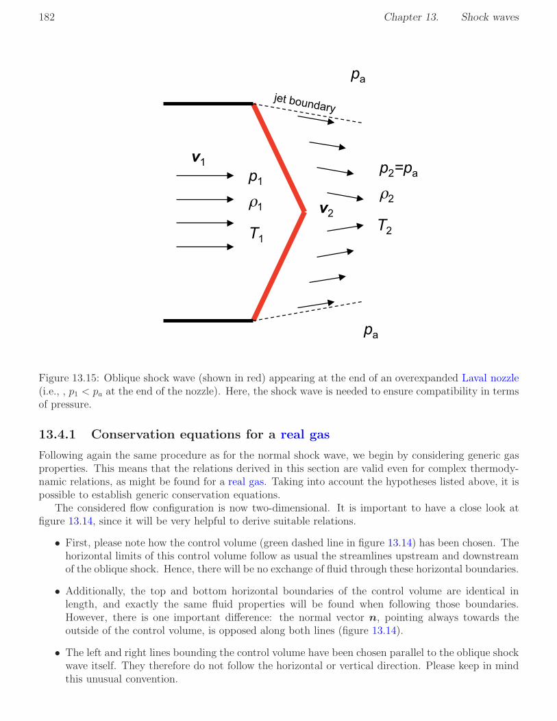
182 Chapter 13. Shock waves
v1
v2
p1
1
T1
p2=pa
2
T2
pa
pa
jet boundary
Figure 13.15: Oblique shock wave (shown in red) appearing at the end of an overexpanded Laval nozzle(i.e., , p1 < pa at the end of the nozzle). Here, the shock wave is needed to ensure compatibility in termsof pressure.
13.4.1 Conservation equations for a real gas
Following again the same procedure as for the normal shock wave, we begin by considering generic gasproperties. This means that the relations derived in this section are valid even for complex thermody-namic relations, as might be found for a real gas. Taking into account the hypotheses listed above, it ispossible to establish generic conservation equations.
The considered flow configuration is now two-dimensional. It is important to have a close look atfigure 13.14, since it will be very helpful to derive suitable relations.
• First, please note how the control volume (green dashed line in figure 13.14) has been chosen. Thehorizontal limits of this control volume follow as usual the streamlines upstream and downstreamof the oblique shock. Hence, there will be no exchange of fluid through these horizontal boundaries.
• Additionally, the top and bottom horizontal boundaries of the control volume are identical inlength, and exactly the same fluid properties will be found when following those boundaries.However, there is one important difference: the normal vector n, pointing always towards theoutside of the control volume, is opposed along both lines (figure 13.14).
• The left and right lines bounding the control volume have been chosen parallel to the oblique shockwave itself. They therefore do not follow the horizontal or vertical direction. Please keep in mindthis unusual convention.

4 Oblique shock wave 183
• In the same manner, the coordinate system is different from our usual choice: the y-directionfollows again the oblique shock wave; the x-direction is of course perpendicular to the y-axis androughly in flow direction, but it is not horizontal.
• In order to account for this unusual axis system, the flow velocity v has been decomposed intoits normal component vn, normal to the oblique shock wave, and its tangential component vt,parallel to the oblique shock wave. The corresponding vector relation simply reads:
v = vn + vt (13.67)
Now, using the Pythagorean theorem in the right triangle formed by v, vn, vt, one obtains:
v21 = vn12 + vt1
2 (13.68)
v22 = vn22 + vt2
2 (13.69)
Additionally, looking back at figure 13.14, it is easy to recognize that the angle between v and vn isa complementary angle to the shock angle ε. Therefore, using the standard angular relations in a righttriangle, it is possible to write successively:
vn1 = v1 cos (90 − ε) = v1 sin ε (13.70)
vt1 = v1 cos ε (13.71)
vn2 = v2 sin(ε− δ) (13.72)
vt2 = v2 cos(ε− δ) (13.73)
Mass conservation
For the steady flow bounded by the streamtube shown in green in figure 13.2 the mass conservation isagain represented simply by the conservation of the mass flow-rate (m = constant) through any tubecross-section.
Here, all streamlines are parallel to each other, so that the cross-section of the streamtube is constantin spite of the flow deflection (angle δ between inflow and outflow directions), A(x) = A1 = A2 =constant.
There is no fluid leaving or entering the control volume through the horizontal boundaries. On theleft and right side, the boundaries being parallel to the oblique shock wave, only the normal velocitycomponent vn must be taken into consideration. The tangential velocity component vt, being parallelto the boundaries of the control volume, does not lead to any exchange of fluid with the surroundings.
Hence, the mass conservation relating upstream and downstream conditions simply reads:
ρ1vn1 = ρ2vn2 (13.74)
Conservation of momentum
Friction plays obviously no role for the configuration considered in figure 13.14, since there is no velocitygradient upstream and downstream of the discontinuity (homogeneous flow conditions). Therefore, thesuitable expression for conservation of momentum in this two-dimensional, steady compressible flow isthat introduced in Chapter 4 (Eq. 4.17):
∫ ∫
Acf
ρ(x, t)v(x, t) (v(x, t) · n) dA =∫ ∫ ∫
Vcf
ρ(x, t)gdV −∫ ∫
Acf
p(x, t)ndA (13.75)

184 Chapter 13. Shock waves
As usual for a gas flow, the contribution of gravity will be completely neglected due to the low densityof gases, even at relatively high pressure. This vector relation will be written instead using two scalarrelations along the direction x (normal to the shock wave) and y (tangential to the shock wave).
It is clear that all contributions along the horizontal boundaries of the control volume are zero (for thevelocity term, due to the fact that (v · n) = 0) or compensate each other exactly (for the pressure term,due to the opposite directions of n along the top and bottom boundaries). Therefore, the only remainingcontributions in Eq.(13.75) are found along the left and right boundaries. Along the x-direction, thoseterms involve only the normal velocity component, both in v and in the scalar product (v ·n). One thusobtains for momentum conservation along x:
p1 + ρ1v2n1 = p2 + ρ2v
2n2 (13.76)
Considering now the y-direction for the terms along the left and right boundaries, v now involves onlyvt while the scalar product (v · n) still delivers vn, so that the momentum conservation along y finallyreads:
ρ1vn1vt1 = ρ2vn2vt2 (13.77)
Dividing now Eq.(13.77) by Eq.(13.74), one obtains immediately the important relation:
vt1 = vt2 (13.78)
The tangential velocity component vt remains unchanged when crossing the oblique shock wave!
Energy conservation
The conservation of energy is again simply derived from the First Law of Thermodynamics. For such anisolated adiabatic system, the total energy is constant, which can be written when neglecting as usualthe contribution of potential energy for this gaseous flow:
h1 +v212
= h2 +v222
(13.79)
It is identical to that obtained for the normal shock wave.
13.4.2 Conservation equations for a perfect gas
The previous relations are only slightly modified when considering the special case of a perfect gas, asdone in the rest of this section. Using Eq.(11.42), one obtains for:
• Mass conservation (unchanged):
ρ1vn1 = ρ2vn2 (13.80)
• Conservation of momentum in x-direction (unchanged):
p1 + ρ1v2n1 = p2 + ρ2v
2n2 (13.81)
• Conservation of momentum in y-direction (unchanged):
vt1 = vt2 (13.82)

4 Oblique shock wave 185
• Energy conservation:
cpT1 +v212
= cpT2 +v222
(13.83)
On one hand, this relation can be transformed in a manner similar to that done for the normal shockwave, replacing temperature and kinetic energy together using the stagnation temperature T0,leading to:
cpT01 = cpT02 (13.84)
Since cp = constant, it is thus again clear that, in this adiabatic flow, the stagnation temperature T0
is the same upstream and downstream of the oblique shock wave:
T01 = T02 (13.85)
On the other hand, it is also possible to rewrite Eq.(13.83) using again the Pythagorean theoremv2 = vn
2 + vt2 and simplifying the tangential component vt since v2t1 = v2t2, leading finally to:
cpT1 +v2n12
= cpT2 +v2n22
(13.86)
Summarizing, the final conservation equations for mass, momentum (in x-direction) and energy read asa whole:
ρ1vn1 = ρ2vn2 (13.87)
p1 + ρ1v2n1 = p2 + ρ2v
2n2 (13.88)
cpT1 +v2n12
= cpT2 +v2n22
(13.89)
Comparing these equations to those obtained for the normal shock (i.e., comparing Eq.(13.87) toEq.(13.7), comparing Eq.(13.88) to Eq.(13.8) and comparing Eq.(13.89) to Eq.(13.9)), it is easy tosee that both equation sets are identical, provided that the velocities v are replaced everywhere by therespective normal components of the same velocity, vn.
This therefore delivers the practical solution for our problem. When considering an oblique shock, adecomposition of the flow field in directions normal (index n) and tangential (index t) to the shock willbe first realized. Then:
• In the tangential direction, the velocity remains unchanged by the shock: vt1 = vt2.
• In the normal direction, i.e., when considering only the normal components of the velocity, theoblique shock behaves exactly like the normal shock considered in Section 13.2. There is no needto develop a special solution for this problem.
Beware! Unfortunately, this statement does not necessarily apply for relations involving several inter-mediate steps and dynamic flow properties, switching back and forth between velocity magnitude andnormal velocity, or between Mach number and normal Mach number. . . For instance, the shock relationof Prandtl (see Eq.13.42) cannot directly be transformed into a form valid for oblique shocks; in orderto derive a suitable equation, the tangential velocity component must be taken into account as well,limiting its applicability.

186 Chapter 13. Shock waves
13.4.3 Jump relations involving the upstream Mach number M1
As explained above, all the relations derived for the normal shock wave can immediately be used forthe oblique shock wave as long as the normal velocity components vn are used instead of the velocitymagnitude v.
Let us exemplify the process for the pressure jump. We know for the normal shock (Eq. 13.26):
p2p1
=2γM2
1 − γ + 1
γ + 1(13.90)
Now, the flow velocity v does not appear in this equation, so it would be possible to believe that thereis nothing to do. This is indeed misleading. The right answer is that the flow velocity v does notappear directly. But, considering the definition of the Mach number M = v/c, it is clear that the flowvelocity is contained as well within M , every time the Mach number appears. Therefore, it is necessaryto reformulate slightly the rule mentioned previously:
All the direct relations derived for the normal shock wave can immediately be used for theoblique shock wave as long as the normal velocity components vn are used instead of thevelocity magnitude v. This rule applies as well to the Mach number, which must be replacedby the normal Mach number Mn defined as:
Mn :=vnc
(13.91)
As a first step, the relation between the normal Mach numbers upstream and downstream of theshock wave is simply:
Mn2 =
√√√√2 + (γ − 1)M2
n1
2γM2n1 + 1− γ
(13.92)
All the jump relations can be readily obtained for the oblique shock using this same rule. One obtainssuccessively:
• For the pressure jump:p2p1
=2γM2
n1 − γ + 1
γ + 1(13.93)
• For the temperature jump:
T2
T1=
(
2γ
γ + 1M2
n1 −γ − 1
γ + 1
)(
γ − 1
γ + 1+
2
(γ + 1)M2n1
)
(13.94)
• For the density jump:ρ2ρ1
=(γ + 1)M2
n1
2 + (γ − 1)M2n1
(13.95)
• For the velocity jump:v2v1
=2 + (γ − 1)M2
n1
(γ + 1)M2n1
(13.96)
It is not necessary to plot again the corresponding evolutions, since they would be identical to figures13.4 to 13.7 when replacing M1 by Mn1 along the x-axis. The qualitative statements remain the same:the jump in pressure is the most noticeable effect of an oblique shock; pressure and temperature jump

4 Oblique shock wave 187
tend toward infinity when increasing the upstream normal Mach number, while density and velocityjump tend toward a finite limit value.
The analogy can be pursued in a similar manner concerning the stagnation pressure and specific entropy.Concerning in particular this last quantity, it has been demonstrated in Section 13.2.7 that a normalshock can only exist for an upstream Mach number M1 ≥ 1. Using the rule derived previously, thecondition on specific entropy connected to the Second Law of Thermodynamics for the oblique shocknow reads Mn1 ≥ 1.
In order to really understand the meaning of this relation, it is necessary to look back at figure 13.14.Due to geometrical considerations, we have already written Eq.(13.70):
vn1 = v1 sin ε (13.97)
Since Mn := vn/c, the normal Mach number is thus simply:
Mn1 = M1 sin ε (13.98)
Similarly, behind the oblique shock wave, Eq.(13.72) relates normal velocity and velocity magnitude byvn2 = v2 sin(ε− δ), so that the normal Mach number behind the oblique shock is:
Mn2 = M2 sin(ε− δ) (13.99)
The conditions found in Section 13.2.7 for the normal shock (M1 ≥ 1 before the normal shock, andtherefore M2 ≤ 1 after the normal shock) are therefore written for the oblique shock: Mn1 ≥ 1 andMn2 ≤ 1. Taking into account the angular relations written above, one obtains finally upstream of theoblique shock
M1 sin ε ≥ 1 (13.100)
Since (sin ε) is obviously below 1, this relation therefore necessitates as well M1 ≥ 1. As a consequence,the statement listed in Section 13.2.7 for the normal shock remains valid: a steady oblique shock canonly exist in a supersonic flow.
The situation is different after the oblique shock. The corresponding condition reads:
M2 sin(ε− δ) ≤ 1 (13.101)
But, since again sin(ε − δ) is obviously below 1, this condition does not necessitate M2 ≤ 1. As aconsequence and as will be shown later, the Mach number M2 behind the oblique shock can be eithersupersonic or subsonic. In practice, the supersonic regime is often found, though the subsonic regimeexists as well. Finally, there is no clear rule concerning the value of M2 behind the oblique shock, apartfrom the fact that M2 must be always smaller than M1 (deceleration induced by the shock wave).
13.4.4 Summary: evolution of all quantities through an oblique shock
All observations described in the previous sections are summarized in Table 13.2, which is nearly identicalto Table 13.1, apart for the fact that the Mach number M2 behind the oblique shock can be eithersupersonic or subsonic.
13.4.5 Using the shock tables for an oblique shock
As discussed previously, all the relations derived for the normal shock wave can immediately be usedfor the oblique shock wave as long as the normal velocity components vn are used instead of the ve-locity magnitude v. This rule applies as well to the Mach number, which must be replaced by thenormal Mach number Mn.

188 Chapter 13. Shock waves
Quantity EvolutionT0 T01 = T02
M (from M1 ≥ 1) ց (M2: subsonic or supersonic)v v1 ց v2p p1 ր p2p0 p01 ց p02T T1 ր T2
s s1 ր s2
Table 13.2: Evolution of the main flow quantities through an oblique shock wave
Therefore, the tabulated values listed in Appendix F for the normal shock (in the case γ = 1.4)can be used for the oblique shock, provided the normal Mach number Mn1 = M1 sin ε (and not theMach number!) is used to enter the Table in the first column (entitled M). Then:
• the eighth column gives the normal Mach number Mn2 = M2 sin(ε − δ) downstream of the shockwave (and not M2!);
• the ninth column gives the pressure jump through the oblique shock;
• the tenth column gives the density jump;
• the eleventh column gives the temperature jump;
• the twelfth column gives the jump in stagnation pressure.
13.4.6 Determining the shock angle ε
Now, it is clear that the normal velocity vn and even more the normal Mach number Mn must beknown to solve the problem. Since Mn1 = M1 sin ε, the only real unknown is the shock angle ε. Arelation is needed to compute this angle. For this purpose, it is appropriate to start again from the massconservation, Eq.(13.87), rewritten as:
ρ2ρ1
=vn1vn2
(13.102)
Now, combining Eq.(13.70) with Eq.(13.71), it is easy to see that:
vn1 = vt1 tan ε (13.103)
Using now Eq.(13.72) with Eq.(13.73), one obtains in the same way:
vn2 = vt2 tan(ε− δ) (13.104)
Considering those last two relations, Eq.(13.102) can now be rewritten:
ρ2ρ1
=vt1 tan ε
vt2 tan(ε− δ)(13.105)
Keeping in mind Eq.(13.78), vt1 = vt2, this equation simplifies to:
ρ2ρ1
=tan ε
tan(ε− δ)(13.106)

4 Oblique shock wave 189
Using Eq.(13.95) to replace the density jump and exchanging left-hand and right-hand side, it comes:
tan ε
tan(ε− δ)=
(γ + 1)M21 sin
2 ε
2 + (γ − 1)M21 sin
2 ε(13.107)
Using now the standard trigonometric relation:
tan(φ− ϕ) =tanφ− tanϕ
1 + tanφ tanϕ(13.108)
it is slightly tedious but straightforward to reformulate Eq.(13.107) into:
1
tan δ=
(γ + 1)M2
1
2(
M21 sin
2 ε− 1) − 1
tan ε (13.109)
Hence, providing a value for the deflection angle δ and the upstream Mach number M1, Eq.(13.109) canbe used to compute the corresponding value of the shock angle ε. This has been done in figure 13.16,where even more information has been shown:
• Only the lower part of the diagram, plotted in solid red and blue lines, should be considered. Itcorresponds to so-called weak solutions, and those are the ones we are presently computing. Theupper part, associated to strong oblique shock waves, is far less relevant for practical purposes andwill not be further discussed.
• Following now one line M = constant, a turning point is observed for some value of the deflectionangle, δ = δmax(M). The corresponding value is marked in figure 13.16 with ∗. The existence ofδmax(M) shows that there is a maximum possible deflection in any supersonic flow leading to anoblique shock wave as shown in figure 13.14. When trying to deflect such a supersonic flow byan angle δ > δmax(M), a different physical solution will appear. Since this is not often found inpractice, such a configuration will not be further considered in what follows.
• Finally, following again one line M = constant, a + symbol is plotted slightly below the ∗ symbol.This is the limit beyond which a subsonic flow (M2 < 1) will be found after the oblique shock. Forvalues of ǫ below the + symbol, the flow beyond the oblique shock wave is supersonic (M2 > 1).In-between the + and the ∗ symbol, subsonic conditions are found downstream of the obliqueshock (M2 < 1).

190Chapter
13.
Shock
waves
0 4 8 12 16 20 24 28 32 36 40 44 48 0
10
20
30
40
50
60
70
80
90
11.05
1.1
1.15
1.2
1.25
1.3
1.35
1.4
1.45
1.5
1.6
1.7
1.8
1.9
2 2.2
2.4
2.6
2.8
3 3.23.43.6
4 4.55 6 8 1020
Deflection angle δ (in °)
Sh
ock a
ng
le ε
(in
°)
Figu
re13.16:
Grap
hical
relationbetw
eenthedeflection
angle
δ(x-ax
is)an
dtheshock
angle
ε(y-ax
is)as
afunction
oftheupstream
Mach
number
M1(lin
es),corresp
ondingto
thesolu
tionof
Eq.(13.109).
Only
thelow
erpart
ofthediagram
,show
naltern
ativelywith
solidred
andbluelin
es,shou
ldbecon
sidered
.

4 Oblique shock wave 191
13.4.7 Mach angle and Mach wave
It has been discussed previously that the Second Law of Thermodynamics leads to the condition M1 ≥ 1for a normal shock (see Section 13.2.7). The similar condition for an oblique shock is now Mn1 ≥ 1, orM1 sin ε ≥ 1.
Therefore, it is possible to define for any supersonic flow (M ≥ 1) the so-called Mach angle µ by thefollowing relation:
sinµ :=1
M(13.110)
The Mach angle µ is listed in the seventh column of Appendix F for γ = 1.4.Now, an oblique shock wave associated to a shock angle ε = µ automatically leads to the condition
M sin ε = M sinµ = Mn = 1: this is the weakest possible oblique shock, leading to no change at all inthe flow, since under such conditions p2 = p1, T2 = T1, ρ2 = ρ1. . .
An oblique shock wave with the shock angle µ is called a Mach wave. It is an invisible structurepresent in any supersonic flow (remember that the Mach wave does not lead to any change in the flow).An oblique shock wave becoming weaker and weaker (i.e., when Mn1 → 1), for instance because thedeflection angle is progressively reduced (δ → 0) tends toward such a Mach wave. Therefore, measuring(perhaps from a simple picture) the shock angle of a very weak oblique shock wave, produced for instanceby a minute deflection, it is possible to determine indirectly the Mach number of the flow by
M = limδ→0
(1
arcsin ε
)
(13.111)
13.5 Polar curve and Busemann diagram
As a final step, it is possible to combine all possible shock waves existing in a supersonic flow by plottingthe polar curve. The objective of this graphical representation is indeed to show at a glance all steadyshock structures that might be found in a supersonic flow with fixed conditions (index 1) upstream ofthe shock. In practice, only the upstream Mach number M1 and the upstream temperature T1 are fixed.As usual, the representation shown in figure 13.17 considers the case γ = 1.4, but a similar picture canobviously be obtained for any value of γ.
The underlying process is as follow:
• Fixing M1, T1 and the gas (air in figure 13.17), the corresponding upstream velocity is fixed aswell by Eqs.(11.29) and (11.51):
v1 = M1
√
γrT1 (13.112)
• The resulting upstream velocity vector v1, which is constant in the present case, is now used todefine the x-axis of the graphical representation. The retained origin for this vector, written Ω, isthe origin of the coordinate system and will be chosen as well as origin to plot all other vectors inthis figure. Note also that there is no need to extend the x-axis beyond v1, since it correspondsto the maximum downstream velocity for any possible shock in this flow.
• Now, the only remaining task is to plot in this same coordinate system the downstream conditionsfor all shocks possibly occurring in this flow for the same gas, Mach number M1 and upstreamtemperature T1. Let us begin with the case where the shock does not lead to any deflection, δ = 0.This means that the velocity vector v2 downstream of the shock is simply parallel to v1 and willtherefore itself be part of the x-axis. There are two possible shock solutions without deflection:
The Mach wave, or “invisible shock’’, leading to no modification at all of the flow. In thatcase, one obtains directly v2 = v1.

192 Chapter 13. Shock waves
The normal shock discussed in Section 13.2. In that case, the downstream velocity is givenby Eq.(13.30), which has been used to compute the velocity magnitude v2 in figure 13.17:
v2v1
=2 + (γ − 1)M2
1
(γ + 1)M21
(13.113)
• Finally, let us consider all further oblique shocks with a real deflection, δ > 0. In that case, thedirection of the vector v2 is already known (angle δ between the x-axis, i.e., the vector v1 andthe downstream velocity vector v2). Only the magnitude is now needed. The computation of v2involves several successive steps:
Knowing M1 and δ, determine the shock angle ε, either graphically from figure 13.16 ornumerically from Eq.(13.109);
Then, compute the normal Mach number Mn1 = M1 sin ε;
The normal Mach number Mn2 downstream of the shock is given by Eq.(13.92):
Mn2 =
√√√√2 + (γ − 1)M2
n1
2γM2n1 + 1− γ
(13.114)
The downstream Mach number is now M2 = Mn2/ sin(ε− δ);
In parallel, the temperature downstream of the shock is given by Eq.(13.94):
T2
T1=
(
2γ
γ + 1M2
n1 −γ − 1
γ + 1
)(
γ − 1
γ + 1+
2
(γ + 1)M2n1
)
(13.115)
Knowing nowM2 and T2, the downstream velocity magnitude can be again directly computedusing Eqs.(11.29) and (11.51):
v2 = M2
√
γrT2 (13.116)
Knowing angle and magnitude, the downstream velocity vector v2 can be finally plotted infigure 13.17.
• Repeating this process for any possible deflection angle δ ≤ δmax (see also figure 13.18), the polarcurve is obtained, as presented in figure 13.17.
Keeping in mind the condition vt1 = vt2 (Eq. 13.78), the polar curve can also be used a posteriorito determine graphically the shock angle ε (see now figure 13.18). For this purpose, it is sufficient tofirst draw the straight line connecting the tip of the upstream velocity vector v1 with the tip of thedownstream velocity vector v2. Drawing now the straight line starting from Ω and perpendicular to thefirst line, it is clear that this second line gives the direction of the oblique shock, since the projections ofv1 and v2 onto this line, which represent the tangential part of those vectors, are equal, hence fulfillingthe condition vt1 = vt2, as written in figure 13.18.
Along the polar curve, the oblique shock waves leading to a supersonic downstream flow are shownin red, while those leading to subsonic downstream conditions are in blue in figure 13.17. It is againvisible that most cases lead to supersonic flows behind the oblique shock.
The maximum possible deflection angle δmax is also directly visible from figure 13.18 (last solutionleading to an oblique shock, i.e., last point along the polar curve – that associated to the lowest velocityv2).
The Busemann diagram is that obtained when representing on the same figure the polar curves for avariety of upstream flow conditions. It can be used to determine all relevant properties of any shock wave

6 Boundary conditions and shock reflections 193
! "!! #!! $!! %!! &!! '!!
"!!
!
"!!
#!!
$!!
( )*+,-./01-,23,4*4/152678
0)*+,-./01-,23,4*4/152678
δ
Ω !!"
!#"
$%&'"
(%)*"
+,-.%/"
0',&1"
*2*.3/%-4"
,5/678*"0',&1"
0850,+6&"
9,(+0:-*%."
;,("
3,/%-"&8-)*"
Figure 13.17: Graphical representation of the polar curve showing all possible shock structures found ina fixed supersonic flow. For the present case, air is considered (γ = 1.4 and r = 287 J/(kg.K)). A Machnumber M1 = 2 has been arbitrarily selected here, together with an upstream temperature T1 = 300 K.
in a flow. Its advantage is that it is a very compact representation: on a single figure, everything can bedetermined. One drawback is the comparatively low accuracy of the obtained information, stemmingfrom the difficulty of reading accurately the value of small angles. Therefore, as far as possible, it isrecommended to use instead the shock tables or – even better – a numerical solution of the equationslisted in this chapter.
13.6 Boundary conditions and shock reflections
Let us first have a look back at figure 13.13, on which the relevant compatibility conditions leadingto shock waves have been explained. Compatibility conditions must be obtained for velocity direction,pressure, and (at least to some extent) velocity magnitude. Very often, these very same boundaryconditions will lead to reflected oblique shocks in practical cases involving walls. To understand thispoint, let us redraw now figure 13.14 with an upper wall, leading to figure 13.19.
Obviously, the deflection obtained after the first oblique shock is not compatible with the upper flow,since the flow would point into the wall, which is unphysical. Therefore, a reflected shock will appearat the contact point between the first oblique shock and the upper wall. The physical purpose of this

194 Chapter 13. Shock waves
! "!! #!! $!! %!! &!! '!!
"!!
!
"!!
#!!
$!!
( )*+,-./01-,23,4*4/152678
0)*+,-./01-,23,4*4/152678
δmax
Ω !!"
!#"
δ axma
ε
Figure 13.18: Graphical representation of the polar curve showing all possible shock structures found ina fixed supersonic flow. For the present case, air is considered (γ = 1.4 and r = 287 J/(kg.K)). A Machnumber M1 = 2 has been arbitrarily selected here, together with an upstream temperature T1 = 300 K.The maximum deflection angle δmax and the graphical procedure used to determine the shock angle ǫare shown as well in this figure.
second shock is to lead back to a horizontal flow, compatible with the (horizontal) direction of the upperwall. But, at the same time, this second shock will lead to a further increase in pressure, temperature,density, as well as to another flow deceleration.
Now, this second shock, when meeting the lower wall, will again be reflected, so that the flowafter the third shock will again be parallel to the lower wall. Those reflections will repeat until perfectcompatibility conditions are reached, or very often, will stop by reaching a last, normal shock wave whenentering a region with parallel walls. The real shock system depends of course on the real geometricalconfiguration.
13.7 Conclusions
Using the relations derived in this chapter, it is now possible to compute all relevant properties for thenormal and oblique shock waves that might be found in any supersonic flow. In fact, there are furtherpossible structures that have not been discussed here; in particular, rarefaction waves will be considered

7 Conclusions 195
v1
v2 p1
1
T1
p2
2
T2
v3
p3
3
T3
Figure 13.19: Typical configuration for the analysis of a fixed, oblique shock wave (shown in red) withboth lower wall (deflection angle δ) and upper wall, leading to (multiple) shock reflection(s) as neededto ensure compatibility in terms of velocity direction.
in a later version of this document; strong shock waves have not been discussed at all, because theytypically do not play an important role in practice; the same applies to discontinuity lines. Still, theconcepts already discussed will be sufficient to obtain a working solution in a vast majority of practicalcases involving supersonic flows!

196 Chapter 13. Shock waves

Chapter 14
Introduction to turbulence
14.1 Turbulence: complexity and importance
Turbulence is an extremely complex issue, which is mostly unsolved at present time. Understandingturbulence is perhaps the most difficult challenge of classical physics, as demonstrated for instance asfollows:
• Sir Horace Lamb was one of the most well-known English scientists at the beginning of the 20thcentury (elected a fellow of the Royal Society in 1884, received its Royal Medal in 1902 and, itshighest honour, the Copley Medal in 1924). He also wrote one book considered as one of the oldestreference works on Fluid Dynamics, which is still reprinted and available in good libraries today[Lam97]. At the end of his career, he commented wittily the challenge of turbulence in an addressto the British Association for the Advancement of Science in 1932:
I am an old man now, and when I die and go to heaven there are two matters onwhich I hope for enlightenment. One is quantum electrodynamics, and the other is theturbulent motion of fluids. And about the former I am rather optimistic.
• Richard Feynman, Nobel Prize 1965, was one of the most talented physicists of the 20th century.He used to write down on a blackboard all the scientific challenges he had to solve before dying. Ashe died (1988), there was only one such challenge left, apart from issues associated with quantumtheory: “non-linear classical hydrodynamics”, another expression to describe turbulence. . .
• the Clay Mathematics Institute introduced in 2000 seven key problems called “Millenium PrizeProblems”. Any scientist solving one of these problems will receive immediately 1, 000, 000 $.From the seven issues considered, only one comes from physics: demonstrating the existence of aunique solution for the Navier-Stokes equation (see Chapter 9). This is again one problem directlyassociated with turbulence, since it has been shown numerically that the Navier-Stokes equationis suitable to describe turbulent flow features.
As a summary, the scientist who will solve the problem of turbulence will certainly receive the NobelPrize in Physics within few years! Top level researchers have been looking for a solution during at least150 years, and this appears to be the most difficult issue left for classical physics.
Then, why do we care? If this is so difficult, let’s forget it completely! Well, this will not be possible.As a matter of fact, an overwhelming majority of practical applications involving flows take place inthe turbulent regime. This is of course only an order of magnitude, but, looking at the most well-known Fluid Dynamics problems, one could state that roughly 90% of all flows of interest are turbulentflows (for exceptions, see next section). Therefore, it is easy to understand that we have to considerturbulence, in spite of the challenge it represents.
197

198 Chapter 14. Introduction to turbulence
14.2 A first taste of turbulence: the experiment of Reynolds
In an extremely famous experiment, Obsorne Reynolds paved the way for a first feeling of turbulence.He observed the mixing process between a tracer (ink) and plain water, flowing parallel to each other,as a function of the velocity of both streams. In this manner, he was able to demonstrate that:
• at low velocity, the mixing was extremely slow, both streams flowing further parallel to each otherin a very regular manner. We will call these conditions laminar from now on.
• at intermediate velocity, both fluids were still well separated (limited amount of mixing), but wereshowing clearly visible vortex structures, impacting the flow direction in space and time. We willcall these conditions transitional.
• finally, at high velocity, both fluids were mixed very rapidly, and the mixing process involved verycomplex, chaotic, unstructured vortices at different scales. We will call these conditions turbulent.
In later experiments it could be demonstrated that these modifications are not only connected to anincrease of velocity. As explained in the chapter dealing with non-dimensional parameters (Chapter 10),isolated flow parameters are not essential and should be grouped to remove dimensions. In this manner,the Reynolds number Re has been defined:
Re :=ρvl
µ=
vl
ν(14.1)
involving a characteristic velocity v, a characteristic length-scale l, a characteristic viscosity (eitherdynamic µ or kinematic ν), possibly a characteristic density ρ.
Since l and ν have been kept constant in the experiment of Reynolds, his observations can be re-stated as follows. A flow is laminar for small values of the Reynolds number Re, turbulent for largevalues of Re, transitional in between (figure 14.1).
Reynolds number
Res
0
laminar
flow
turbulent
flow
Value depends on
application and on the
retained length scale s
∞
transition
Figure 14.1: Impact of the Reynolds number Re on the flow conditions.
Considering the definition of the Reynolds number, Eq.(14.1), it is easy to determine the impactof different quantities on the flow state. Considering Table 14.1, one can identify the few flows thatwill not take place in the turbulence regime: slow flows at small scales and/or involving highly viscousfluids. These might be for instance micro-scale flows, like found in fuel cells, for which tubes of a few

3 Qualitative properties of turbulent flows 199
Variable More laminar More turbulent(Less turbulent)
Velocity v Reduce v (slow flow) Increase v (fast flow)Scale l Reduce l (small-scale flow) Increase l (large-scale flow)
Viscosity Increase viscosity (highly viscous flow) Reduce viscosity
Table 14.1: Influence of different quantities on the flow state and on the transition between laminar andturbulent conditions
100 µm are typically employed. Since micro-scale flows lead to very high viscous effects, they usuallyinvolve very small velocities, supporting again establishment of laminar conditions. Such laminar flowsat small-scales are also found in the human body, for example blood flows in small vessels. Another caseof laminar flows is found for highly viscous fluids, for example polymers.
14.3 Qualitative properties of turbulent flows
Even if it is difficult to define precisely turbulent flow conditions, a few key properties can be listed andemployed to delineate between laminar and turbulent flows.
• turbulent flows are chaotic, i.e., unpredictable on a long time-scale. An infinitesimally smallperturbation of the system will grow exponentially with time and lead to a completely differentflow solution after some time. The behavior of turbulent flows thus appears to be random, eventhough they are deterministic (i.e., described by known conservation equations). More detailsconcerning chaos theory can be found for instance under Wikipedia.
• turbulent flows lead to a much faster homogeneization for all flow quantities, for example for veloc-ity, temperature or concentration. Therefore, such turbulent flows may be very beneficial for a widerange of practical applications. If you want to mix two different species, or to get a homogeneoustemperature when mixing one cold and one hot jet, this will take place much more efficiently andmuch faster under turbulent conditions, compared to a purely laminar homogeneization process.
• turbulent flows develop as a result of natural instabilities (consider for example the transition toturbulence of a smoke plume after a short way in a quiet surrounding atmosphere) and/or ofuser-induced fluctuations in flow quantities (as done for example when stirring the flow with animpeller).
• turbulent flows can transform back into laminar flows under the influence of viscosity. Indeed,viscosity is a sink term in the conservation equation describing the kinetic energy of turbulence.As a consequence, viscous effects lead to a damping of turbulent structures. The correspondingkinetic energy is of course not lost (energy is always a conserved quantity), but is transformed intothermal energy (temperature increase in the flow).
• turbulent flows always involve vortical structures (vortices), associated with a variety of time-scales(slow up to fast vortices), of length-scales (small up to large vortices) and of orientation.
• turbulent flows are always unsteady. Time-dependent variations of the main flow quantities (alsocalled fluctuations of these quantities) will usually be far from negligible. As a typical order ofmagnitude, relative fluctuations of velocity magnitude with time will often be around 10% in aturbulent flow, sometimes even much more.

200 Chapter 14. Introduction to turbulence
• turbulent flows are always spatially three-dimensional in nature. Even if the main flow characteris-tics can often be approximated as being one-dimensional or two-dimensional, the flow fluctuationsassociated with turbulence will always rapidly develop into a fully three-dimensional field, oftenwithout (isotropic), sometimes with (anisotropic) preferred directions. Note that it is indeed pos-sible to produce in the laboratory and under well-controlled conditions two-dimensional turbulentflows; this is useful for our fundamental understanding but does not correspond to practical flows.
Finally, you understand again why turbulent flows are so complex. In order to simplify our analysis,we have always employed in the past one or more of the following assumptions: reduced dimensionality(one-dimensional flow, two-dimensional flow); steady flow; irrotational flow; incompressible flow. Thelast one is the only remaining assumption that could still safely be used when considering turbulentflows. In principle, the first three ones are wrong from the start, even if they might still be employed toget a first, approximate understanding of what happens in a turbulent flow.
Further information will be found in later versions of this document.

Appendix A
Basic concepts and keywords of fluiddynamics
This chapter is a gathering of the most important concepts and keywords used in the rest of thedocument. It is ordered alphabetically. Usually, you will simply access specifically one or of the otherof the sections by following the appropriate links in the main text.
A.1 Archimedes number
The Archimedes number is the non-dimensional parameter of Fluid Dynamics (see Chapter 10) used toquantify the influence of buoyancy. It is defined as:
Ar :=gl3ρf (ρb − ρf )
µ2(A.1)
and involves the typical size l of the object, and the difference in density between fluid ρf and body ρb.Note that this Archimedes number can be either positive or negative.
Further information can be found for instance under Wikipedia.
A.2 Cavitation
Cavitation is a transition of state between liquid and gas phase, similar to boiling but associated witha change in pressure and not in temperature. For boiling, increasing the temperature of a liquid allowsto travel in the phase space from the liquid phase to the gas phase, keeping the pressure constant.
Similarly, for cavitation, decreasing the pressure of a liquid allows to travel in the phase space fromthe liquid phase to the gas phase, keeping the temperature constant. The corresponding cavitationpressure pc (saturated vapor pressure) associated to the transition between a liquid and a gas dependsof course on the liquid, on the temperature, but also in practice very much on possible impurities presentin the liquid and on the possible existence of suitable seeds promoting cavitation.
The appearance of cavitation is by itself not a real problem. But the resulting bubbles usually collapseback to the liquid phase when encountering a higher pressure at some later point of the flow. Suchcollapsing bubbles induce very intense shock waves in the liquid, and the resulting pressure variationsmay damage very rapidly any wall or structure placed in the vicinity. Due to this structural damage,cavitation must usually be avoided.
Depending on water purity and on the temperature, the critical cavitation pressure pc for water hasan order of magnitude pc ≈ 0.01 bar (hundred times smaller than typical atmospheric pressure).
201

202 Appendix A. Basic concepts and keywords of fluid dynamics
True cavitation involves thus a two-phase mixture of a liquid with its own vapour. The somewhatsimilar, but less harmful process called pseudo-cavitation appears when a gas (for instance air) dissolvedin a liquid leads to the formation of bubbles in this liquid at some point in the flow where low pressuresare found. In that case, we observe again a two-phase flow (liquid/gas), but the gas is not the vapourof the liquid.
Further information can be found for instance under Wikipedia.
A.3 Compressible flow
Throughout this document, a flow is called compressible if the change of density induced by a modifi-cation of pressure (and thus indirectly of velocity) cannot be neglected. Further details can be found inthe section dealing with the opposite notion, incompressible flows.
A.4 Compressible fluid
Throughout this document, a fluid is called compressible if it is possible at all to change its density.Further details can be found in the section dealing with the opposite notion, incompressible fluids. Notethat, in reality, all fluids are in fact compressible, at least to some extent.
A.5 Conservative force
A force is called conservative if the work associated with the action of this force is independant fromthe way followed during the movement, but only depends on the starting point and endpoint of thisdisplacement. All the non-contact forces considered in this document are conservative and their localaction on the fluid can be written ρk, with k the corresponding acceleration vector. Mathematically,such a force is conservative if it meets one of the two following, equivalent conditions:
∇× k = 0 or (A.2)
k = −∇φ (A.3)
where φ is the scalar field of potential energy associated with the considered acceleration vector. Con-sidering as an example the earth gravity field using the standard coordinate system, one obtains
φ(x) = φ(z) = gz (A.4)
and consequentlyk = −∇φ = −gez = g (A.5)
Further information can be found for instance under Wikipedia.
A.6 Contact force vs. non-contact force
Throughout this document, a contact force is defined as a force that can only be active between twofluid elements in direct contact with each other. This is distinct from a non-contact force (a force thatacts over a long distance), such as gravity. From a fundamental point of view, this is a somewhatinaccurate view of the real physics. It will nevertheless be useful to separate between long-range forces(for us, in particular gravity) and forces, which take place only when two fluid elements are in directvicinity to each other (this will concern for us mainly the pressure force and to a lesser extent the forceassociated to surface tension).
Further information can be found for instance under Wikipedia.

7 Hydraulic diameter 203
A.7 Hydraulic diameter
For a cylindrical pipe, it is obviously a straightforward task to dermine its diameter d. For a non-cylindrical cross-section, it is then useful to introduce an equivalent diameter, called in practice hydraulicdiameter dh and defined as:
dh :=4A
Pw
(A.6)
and connecting the cross-section area A (in m2) with the wetted perimeter (or contact length betweenfluid and wall) Pw (in m). As a result, the hydraulic diameter has obviously the right dimension. For acylindrical tube, A = πd2/4 while Pw = πd, so that dh = d, as expected!
The concept of hydraulic diameter, as defined by Eq.(A.6) can now be used for any complex geo-metrical cross-section. For a few standard cases, the computed hydraulic diameter for internal flows isas follows:
square cross-section, side-length l dh = l
rectangular cross-section, side-lengths l1 × l2 dh =2l1l2l1 + l2
equilateral triangular cross-section, side-length l dh =l√3
flow between two infinite parallel plates, separation distance l dh = 2lenclosure between two concentric cylinders, diameters d1 < d2 dh = d2 − d1
For an open channel flow, the top part of the fluid does not lead to any shear stress and is thereforenot included in the computation of the wetted perimeter Pw. As a consequence, the hydraulic diameteris now dh = 4(lH)/(l+ 2H), with H the height of the liquid and l the side length of the flow. If we areconsidering a film or a shallow flow (H ≪ l), this simplifies to dh ≈ 4H .
Finally, note that the concept of hydraulic diameter is not an exact description of the underlyingphysics. It is just an adequate procedure to re-use the measurements results presented for a cylindricalpipe in the Moody-Colebrook chart (figure 6.5) when the cross-section looks different. Due to this poorphysical background, errors must be expected. The errors observed for non-cylindrical cross-sectionsare indeed considerable (20% or more) in the laminar regime. They are usually quite small (a few %) inhighly turbulent flows, due to the diminishing importance of the exact geometry under such conditions.
A.8 Incompressible flow
Throughout this document, a flow is called an incompressible flow if the change of density induced bya modification of pressure (and thus indirectly of velocity) can be safely neglected. This definition issomewhat inaccurate, since it involves a user-dependent threshold (what may be “neglected” or not?).As such, the notion of incompressible flow should not be confused with the clear (even if somewhatirrealistic) notion of incompressible fluid (see next section):
• an incompressible fluid always leads to an incompressible flow;
• but an incompressible flow can involve an easily compressible fluid, for instance a gas like air.
For a compressible fluid, the notion of compressible vs. incompressible flow will be clarified in the chapterdealing with one-dimensional, isentropic compressible flows. We will prove in particular in Chapter 11that the relative change of density ρ induced indirectly by a corresponding relative change of the velocitymagnitude v reads:
dρ
ρ= −M2dv
v(A.7)

204 Appendix A. Basic concepts and keywords of fluid dynamics
M (dρ/ρ)/(dv/v) (in %)0 00.1 10.2 40.3 90.4 160.5 251 100
Table A.1: Ratio between the relative variation of density and the relative variation of velocity magnitudeas a function of the Mach number M
where the Mach number M appears as a key quantity. As a function of the Mach number, the ratiobetween the relative variation of density and the relative variation of velocity magnitude can then bedirectly computed, leading e.g. to Table A.1.
Now, the threshold can be defined more clearly. If, as usual for engineering purposes, 10% is con-sidered as some kind of “magical limit” under which an effect can be neglected, then a Mach numberof 0.3 (strictly speaking, of 0.333 . . .) corresponds to the limit between incompressible (M ≤ 0.3) andcompressible (M > 0.3) flows. If, for some reason, the accuracy of the computation must be very high,so that only a maximal error of 1% can be tolerated, then incompressible flows take place only up toM = 0.1. This is illustrated in figure A.1.
The opposite of an incompressible flow is called a compressible flow.
Mach number
M
10 0.3
subsonic supersonic
sonic
incompressible
flow
compressible
flow
0.1
Value depends on accuracy
requirements, typically
between M=0.1 and 0.3
Figure A.1: Compressible vs. incompressible flow conditions.
A.9 Incompressible fluid
Throughout this document, a fluid is called an incompressible fluid if it can be considered that it isimpossible to change its density ρ by any means, i.e. ρ = constant for any realizable thermodynamicconditions. This is of course only an assumption, there is no perfectly incompressible fluid (in the sense

9 Incompressible fluid 205
of this definition) in reality. This will nevertheless be a very good approximation for most simple liquidsat nearly constant temperature (figure A.2). For example, pure water at ambient temperature is a closeapproximation of an incompressible fluid with ρ ≈ 1000 kg/m3. The notion of incompressible fluidshould not be confused with the notion of incompressible flow (see previous section).
air water
p =
p
Figure A.2: A gas is typically easily compressible, a liquid shows a nearly constant density when varyingpressure.
To be more accurate, the compressibility of a fluid at constant temperature T is defined in fact withthe isothermal compressibility coefficient as
βT :=1
ρ
(
∂ρ
∂p
)
T
(A.8)
while its thermal expansion at constant pressure is defined with the isobaric thermal expansion coefficientas
αp := −1
ρ
(
∂ρ
∂T
)
p
(A.9)
With these concepts, we can now finally clarify what is an incompressible fluid: it is a fluid with βT = 01/Pa and simultaneously αp = 0 1/K. Once again, such a fluid does not really exist. But standard waterunder ambient conditions shows for example an extremely small isothermal compressibility coefficient,βT ≈ 0.5 1/GPa or ≈ 5 10−10 1/Pa, meaning that it is extremely difficult to change the density of waterby changing its pressure at constant temperature. At the same time, its thermal expansion coefficient atconstant pressure and 20C is roughly αp ≈ 2 10−4 1/K, showing again that it is quite difficult to changedensity by changing temperature at constant pressure, even if αp is far from being 0 (in fact, for a liquid,this is even a relatively large value). Therefore, as a whole, liquid water can be safely considered as anincompressible fluid as long as temperature does not change too much and as long as pressure does notreach extreme values.
Further information on the topic can be found for instance under Wikipedia. Additional detailsconcerning thermal expansion are given under Wikipedia/Thermal expansion.

206 Appendix A. Basic concepts and keywords of fluid dynamics
A.10 Internal flow
A flow is called an internal flow if it is everywhere surrounded sideways by solid walls. The typicalexample of an internal flow is the flow within a duct, pipe or channel. Of course, in most cases, therewill still be openings somewhere to allow the flow to enter and/or leave this duct or channel.
A.11 Irrotational flow
A flow is called irrotational flow if the curl of the corresponding velocity field v is zero:
∇× v = 0 (A.10)
Further information can be found for instance under Wikipedia.
A.12 Laminar flow
It is difficult to give an exact and simple definition of a laminar flow, in particular for beginners. Let usstate simply here that a laminar flow is a smooth, regular, simple flow. The evolution of a laminar flowwith time can be predicted with a very high accuracy (laminar flows are predictable).
The contrary of a laminar flow is a turbulent flow, as described in Chapter 14.Further information can be found for instance under Wikipedia.
A.13 Mach number
The Mach number is the most important non-dimensional number for compressible flows. It is definedas the ratio between the magnitude of flow velocity v and local speed of sound c. It is therefore a scalarfield variable, that will usually depend on space and time, M(x, t).
M :=v
c(A.11)
Further information can be found for instance under Wikipedia.
A.14 Multiphase flow
A multiphase flow is a flow involving different fluids that cannot be perfectly mixed at molecular level.This might be for example a spray (liquid droplets transported by a gas phase), a crystallization reactor(solid crystals transported by a liquid) or a sooty flame (solid soot particles transported by a gas); allthese are two-phase flows. A three-phase flow might be for example found in an internal combustionengine, where liquid fuel droplets will burn with (gaseous) air and produce among other solid particlesof soot; or when considering a fluidized bed involving spray coating (liquid droplets interacting withsolid particles in a gas flow).
A.15 Newtonian fluid
A Newtonian fluid is a simple fluid, for which the relation between the shear force applied on the fluid(more rigorously, the associated shear stress) and the resulting deformation of this fluid is linear andgoes through the origin. The associated proportionality constant (slope of the straight line) is the

16 Non-Newtonian fluid 207
Substance Dynamic viscosity µ (Pa s)Air 10−5
Water 10−3
Mercury 1.5 10−3
Olive oil 10−1
Glycerin 1.5Liquid honey ≈ 10Corn syrup ≈ 100Molten polymer ≈ 1000Molten glass ≈ 1012
Table A.2: Order of magnitude of the dynamic viscosity for different Newtonian fluids at room temper-ature [Chh07]
dynamic viscosity of the fluid; as described later, viscosity is one key fluid property, which is a functionof temperature, but stays constant for an isothermal process and for a Newtonian fluid.
Pure water, air and any ideal gas can be considered as Newtonian fluids; but also most gases, manyliquids of low molar mass, molten salts, most liquid metals. . . are at least approximately behaving likeNewtonian fluids. As a consequence, the study of these Newtonian fluids covers a lot of practicalapplications.
Even if Newtonian fluids show a similar qualitative behavior, human beings might get a differentfeeling, simply due to a widely varying viscosity (Table A.2).
The contrary of a Newtonian fluid is a non-Newtonian fluid.
Further information can be found for instance under Wikipedia.
A.16 Non-Newtonian fluid
A non-Newtonian fluid is a fluid associated with more complex properties compared to a Newtonian fluid.For a non-Newtonian fluid, the relation between the shear force applied on the fluid (more rigorously,the associated shear stress) and its resulting deformation is not linear and/or does not go through theorigin.
Examples of non-Newtonian fluids are blood, toothpaste, many alimentation products like ketchup,many cosmetics, heavily-loaded suspensions. . .
Further information can be found for instance under Wikipedia.
A.17 Non-viscous flow
Per definition, a non-viscous flow is a flow for which the influence of viscosity is considered negligible andwill therefore not be further taken into account. Note that this kind of flow, if in addition incompressible,is often called “ideal flow” in the literature. Since this is a source of confusion with the ideal gas, theterm “ideal flow” will never be used in this document and will be replaced by the term “potential flow”.
Since kinematic viscosity is in fact the diffusion coefficient of momentum in the fluid, this approx-imation is indeed exact for all flow conditions associated with a uniform momentum, for example forhydrostatics and aerostatics (momentum equals zero everywhere) or for a fully homogenenous flow (samemomentum everywhere).

208 Appendix A. Basic concepts and keywords of fluid dynamics
A.18 One-dimensional flow
Throughout this document, a flow is called one-dimensional if all flow variables depend in space onlyon one spatial coordinate, a scalar value written x, and not as usual on a vector position x involvingthree components: φ = φ(x) instead of φ = φ(x). Note that one-dimensional flows do not really exist inpractice (they could at best exist for some limited sub-region of the flow) and constitute only a practicalapproximation.
A.19 Open channel flow
As already expressed in the name, an open channel flow is a liquid flow with a top surface in contactwith the surrounding atmosphere. Due to molecular processes taking place along the gas/liquid contactsurface, there is no shear stress acting there. Typical examples of open channel flows are the water flowin a river or a gravity-driven film flow along an inclined plate.
A.20 Potential flow
A flow is called a potential flow if a scalar function φ(x) can be found that satisfies:
∇φ = v (A.12)
where v is the velocity field associated with this flow. Using suitable mathematical relations, it is possibleto demonstrate that this condition is equivalent to the fact that the corresponding flow is irrotational. Inthe chapter, dealing specifically with potential flows, we will assume further that these flows are alwaysincompressible flows, which is very often done in practice and leads to particularly simple solutions.
Further information can be found for instance under Wikipedia.
A.21 Quasi-steady flow
A flow is called a quasi-steady flow if the flow parameters change with time (this is therefore not asteady flow!) but if simultaneously the instantaneous solution obtained for these flow variables (pressure,velocity, density. . . ) is identical to the solution that would be in principle obtained for the correspondingsteady flow at the same instant in time. In other words, a quasi-steady flow is an unsteady flow describedas a succession in time of equivalent steady flow solutions. This corresponds for example to a barrel fullof water being slowly emptied by a small opening in the bottom.
The concept of a quasi-steady flow is extremely useful in practice. Most practical flows are indeedunsteady. But, if they can be assumed to be quasi-steady, all the results developed for steady flows areequally valid for such quasi-steady conditions, as long as they are only used at a fixed time instant.
A.22 Speed of sound
The speed of sound c is the speed at which a small pressure perturbation travels in a compressiblefluid (for an incompressible fluid, the speed of sound would be infinite, which demonstrates again thatincompressible fluids do not really exist in practice and constitute only a practical approximation). Thespeed of sound is used in the definition of the Mach number.

23 Standard coordinate system 209
For a generic fluid, the square of the speed of sound is defined as the ratio between pressure change anddensity change between two thermodynamic states of this fluid related by an isentropic transformation:
c2 :=
(
∂p
∂ρ
)
s
(A.13)
Further information can be found for instance under Wikipedia.
A.23 Standard coordinate system
Throughout this document, we consider that the spatial domain is associated with an orthonormal,Cartesian coordinate system involving three spatial directions, denoted either x = (x, y, z) or (x1, x2, x3),as represented in figure A.3.
Further information can be found for instance under Wikipedia.
x
y
z
x
y
z
O O
Figure A.3: Standard coordinate system.
A.24 Steady flow
Throughout this document, a flow is called steady if all flow variables do not depend on time t, butonly on the spatial position x. As a consequence, the time derivative of any flow-related quantity φ isobviously 0:
∂φ
∂t= 0 (A.14)
By averaging all flow variations in time, a real, time-dependent flow can be of course reduced to asteady flow; but this is only a simplified approximation of reality. The opposite of a steady flow isan unsteady flow; for practical purposes, this is the general case. A very interesting complementarycategory is that of quasi-steady flows.

210 Appendix A. Basic concepts and keywords of fluid dynamics
A.25 Stress in a fluid
Generally speaking, the stress is the ratio between a force and the area A of the geometrical surface Aonto which this force is acting. As such, it is a vector quantity with components expressed in Pascal(Pa), equivalent of N/m2.
x1 O
x2
A
B C
D
p1
p2
21
12
Figure A.4: Concepts of normal and shear stress.
A shear stress corresponds to the case where the force is acting in the tangential plane of thecorresponding surface A (arrows tangential to the cubic fluid volume in figure A.4).
A normal stress corresponds to the case where the force is acting in the normal direction of thecorresponding surface A (arrows normal to the cubic fluid volume in figure A.4).
Let us now consider in more detail the infinitesimal cubic element of fluid medium shown in figure A.4,which has the point of interest at its center and whose square faces, of side-length d, lie perpendicular tothe cartesian axes x1, x2 (and x3 perpendicular to the page). The arrows labelled p1 and p2 in the figureindicate forces, of magnitude d2p1 and d2p2 respectively, exerted on the cube of fluid by two normal stresscomponents, also called pressures, which act on the planes AB and BC. The arrows labelled σ21 andσ12 indicate forces of magnitude d2σ21 and d2σ12 respectively, exerted on the cube of fluid by two shearstress components acting on the same planes; here, the first suffix indicates the direction of the forceand the second the direction of the normal to the plane under consideration. Unlabelled arrows indicatebalancing forces which are exerted on the opposite faces CD and DA. The balance must obviously beexact in the limit d → 0 (infinitesimal volume): any difference between say p1 on one side and thecorresponding pressure p′1 on the opposite side would result in a force proportional to d2 acting on amass proportional to d3 (volume). For d → 0, this would induce infinite accelerations which, as a result,

26 Turbulent flow 211
would eliminate immediately the pressure difference.
A similar argument shows that σ21 and σ12 must always be equal. If they were not equal, the cubewould experience a torque about the x3-axis of magnitude varying like d3(σ21 − σ12), and the resultantangular acceleration would again be infinite for d → 0 because the moment of inertia of the cube isproportional to d5. Hence, the shear stresses are always symmetric. The associated shear stress tensorσ of components (σij) is hence also symmetric:
σ = σT (A.15)
Cutting now our cube in two halves along the diagonal (AC) and producing in this manner twoprisms, BAC and DAC, the same procedure can be repeated for the two resulting, infinitesimal prisms.Since the stress components acting on the prisms can be directly deduced from those acting on theoriginal cube, the same analysis leads finally to the fact that:
p1 = p2 = p3 = p (A.16)
This is a very important observation: the normal stress is simply a scalar quantity, completely describedby an isotropic value, the pressure p. This is sometimes known as Pascal’s theorem.
Further information can be found for instance under Wikipedia.
A.26 Turbulent flow
It is difficult to give an exact and simple definition of a turbulent flow, in particular for beginners.Let us state simply here that a turbulent flow is an irregular, chaotic, complex flow. Such turbulentflows, as described in more detail in Chapter 14, change rapidly with time (unsteady flow) and involvethree-dimensional vortical structures (a turbulent flow is never irrotational). Chaotic means that theevolution of a turbulent flow with time cannot be predicted with a very high accuracy for a longer timescale (turbulent flows will rapidly be unpredictable in the sense of chaotic theory).
The contrary of a turbulent flow is a laminar flow.
Further information can be found for instance under Wikipedia.
A.27 Unsteady flow
A flow is called unsteady if the flow variables are varying with time. If it is nevertheless quasi-steady,then the instantaneous fields of pressure and velocity and still coupled at each instant in the samemanner as in a steady flow, i.e., a flow in which time does not play any role. If it is not quasi-steadyany more, then a completely different instantaneous solution is found.
There is therefore a continuous progression between a steady flow (time plays no role at all), aquasi-steady flow (flow variables are changing with time, but in a similar manner to a steady flow) anda fully unsteady flow (flow variables are changing with time in a different manner as in a steady flow).
A.28 vena contracta
In particular when considering a liquid flow exiting through an opening of surface A, it is very oftenobserved in practice that, shortly after this opening, the effective section of the liquid stream Aeff isindeed lower than the surface A of the opening. This contraction effect is called vena contracta (Latin

212 Appendix A. Basic concepts and keywords of fluid dynamics
name) and has been known for a very long time. This effect is usefully quantified through the contractionratio
Cvc :=AeffA
≤ 1 (A.17)
For a sharp orifice in a straight wall, values of Cvc between 0.6 and 0.65 are typically found.Further information can be found for instance under Wikipedia.
A.29 Viscosity
Two related viscosity concepts will be used in this document. The dynamic viscosity (also called simplyviscosity) is written µ and expressed in kg/(m.s) or equivalently Pa.s. Knowing the density ρ, a relatedquantity called kinematic viscosity, written ν and expressed in m2/s is introduced by
ν :=µ
ρ(A.18)
Physically, the kinematic viscosity is the diffusion coeffient associated with diffusion of momentum in afluid.
Further information can be found for instance under Wikipedia.

Appendix B
Basic thermodynamic concepts needed forfluid dynamics
This chapter is a gathering of the most important thermodynamic concepts needed for a correct under-standing of fluid dynamics. Of course, we cannot go deep into detail! Therefore, only a very superficialdescription of thermodynamic ideas will be proposed here. Hundreds of suitable textbooks can be foundto learn more about thermodynamics.
The chapter is ordered alphabetically. Usually, you will not read this chapter at length, but you willaccess specifically one or the other of the sections by following the appropriate links in the main text.
B.1 Adiabatic process
A change of thermodynamic state is called adiabatic if it takes place without any exchange of heatwith the surroundings. Most (but not all) applications considered in this document will be assumedadiabatic. Since this notion comes from thermodynamics and not primarily from fluid dynamics, wewill not consider it further here.
Further information can be found for instance under Wikipedia.
B.2 Barotropic state
A fluid is in a barotropic state if there is a direct function relating its pressure p to its density ρ:
p = Gp(ρ) (B.1)
or converselyρ = Gρ(p) (B.2)
Further information can be found for instance under Wikipedia.
B.3 Enthalpy
Since the notion of enthalpy comes from thermodynamics and not primarily from fluid dynamics, wewill not consider it in great detail here. Let us state only here that the specific enthalpy h is definedfrom the specific internal energy e of a gas using:
h := e +p
ρ(B.3)
213

214 Appendix B. Basic thermodynamic concepts needed for fluid dynamics
As such, the enthalpy is also the appropriate measure for the energy contained in a compressible gasper unit mass when taking into account pressure changes. We will therefore use the enthalpy instead ofthe internal energy when writing energy conservation in a compressible gas.
One further important relation relates the change of enthalpy dh with the corresponding change ofentropy ds
dh = Tds+dp
ρ(B.4)
through temperature T , density ρ, and associated pressure change dp.Further information can be found for instance under Wikipedia.
B.4 Entropy
Defining in a clear and accurate way the entropy is a major challenge! Since this notion comes fromthermodynamics and not primarily from fluid dynamics, we will not consider it in great detail here. Youwill find plenty of excellent books dealing with this notion [KP98], and sometimes considering nothingelse [Dug96, The07]! For us, let us state only here that the specific entropy s is a measure of the disorderof the fluid system, s increasing when the disorder grows. For an ideal gas, the specific entropy s can bedirectly computed as a function of pressure, density (or temperature) and thermodynamic coefficients.
Further information can be found for instance under Wikipedia.
B.5 Gas constant
In this work, two different gas constants will be employed. The first one, written R, is the universal gasconstant, valid for any gas, and equal to R := 8.314 J/(mol.K). In many cases, it is more practical tointroduce the specific gas constant, written r and related to R by:
r :=R
W(B.5)
where W is the molar mass of the considered gas. As such, r is expressed in J/(kg.K) and is a constantfor a given gas, but depends on this gas. For most examples considered in this document, air will beused. In that case, r = r(air) ≈ 287 J/(kg.K).
Further information can be found for instance under Wikipedia.
B.6 Heat capacity
In principle, the heat capacity describes the capacity of a substance to store heat. The specific heatcapacity is the measure of the heat energy required to increase the temperature of a unit mass quantity(1 kg) of a fluid by a unit temperature interval (1 K). It is therefore logically expressed in J/(kg.K).
Using Mayer’s relation (Eq. B.9) combined with the definition of the specific gas constant (Eq. B.5)in order to eliminate cv, it is easy to obtain for example:
cp =γr
γ − 1(B.6)
Further information can be found for instance under Wikipedia.

7 Heat capacity ratio 215
B.7 Heat capacity ratio
The ratio γ between the specific heat capacity at constant pressure cp and its equivalent at constantvolume (or constant density) cv is an essential thermodynamic parameter, in particular for a gas:
γ :=cpcv
(B.7)
This quantity, sometimes called also isentropic factor or isentropic exponent, is a constant for anideal gas. For many gases under usual conditions, the value of γ can be safely assumed to be con-stant and approximately equal to 1.4.
Further information can be found for instance under Wikipedia.
B.8 Ideal gas
Since the notion of an ideal gas comes from thermodynamics and not primarily from fluid dynamics, wewill not consider it in great detail here. An ideal gas is in principle a gas for which the molecules can beconsidered as point particles interacting with each other only through collisions conserving momentumand energy. Under usual conditions for pressure and temperature, many gases (but not all) behaveindeed very closely like an ideal gas. Usually, this assumption will be violated for either very lowtemperatures, very high pressures, or when supplementary interaction processes occur between the gasmolecules. We will use in this document only a few essential properties of ideal gases:
• An ideal gas obeys the ideal gas law, relating pressure, density and temperature through thespecific gas constant r:
p = ρrT (B.8)
• One mole of this gas (1 mole := 6.02 1023 molecules) occupies roughly 22.4 dm3 (or l) understandard thermodynamic conditions.
• Mayer’s relation between specific heat capacity and specific gas constant:
cp − cv = r (B.9)
Further general information can be found for instance under Wikipedia.
B.9 Isentropic transformation
A change of thermodynamic state is called isentropic if it takes place at constant entropy s. A thermody-namic process that is both thermodynamically reversible and adiabatic is always isentropic. Isentropicflows will always be particularly simple, compared to flows involving a change in entropy.
Further information can be found for instance under Wikipedia.
B.10 Isobaric transformation
A change of thermodynamic state is called isobaric if it takes place at constant pressure p.
Further information can be found for instance under Wikipedia.

216 Appendix B. Basic thermodynamic concepts needed for fluid dynamics
B.11 Isochoric transformation
A change of thermodynamic state is called isochoric if it takes place at constant volume V . Consideringan isolated system (therefore necessarily conserving mass), an isochoric transformation is equivalently atransformation for which the density ρ remains constant.
Further information can be found for instance under Wikipedia.
B.12 Isothermal transformation
A change of thermodynamic state is called isothermal if it takes place at constant temperature T .Further information can be found for instance under Wikipedia.
B.13 Perfect gas
The notion of perfect gas is mostly used in Fluid Dynamics and is therefore not primarily a thermody-namic concept. Per definition, a perfect gas is an ideal gas associated with constant specific heat capacities(cp = constant or cv = constant, this is equivalent). We will use in this document some important rela-tions verified by any perfect gas:
• The specific entropy s of a perfect gas can be computed by
s = cv ln
(
p
ργ
)
+ constant (B.10)
• For an isentropic change of state, following equivalent relations apply, all involving the constantheat capacity ratio γ:
p
ργ= constant (B.11)
T
ργ−1= constant (B.12)
pγ−1
T γ= constant (B.13)
(B.14)
For further information, see Wikipedia.
• The specific enthalpy h of a perfect gas can be computed by
h = cpT + constant (B.15)
By choosing appropriately the reference state, the constant can be removed, leading to
h = cpT (B.16)
B.14 Polytropic process
A thermodynamic process is called a polytropic process if there is a relation between pressure p anddensity ρ following:
p
ρn= constant (B.17)

15 Prandtl number 217
with n the polytropic exponent. Depending on the value of n (with n ≥ 0) and of the gas, differentconditions can be found:
• For n = 0, an isobaric evolution is found (p = constant).
• For n = 1 and for an ideal gas, an isothermal process is necessarily found, since
p
ρ= constant = rT (B.18)
• Finally, for an ideal gas, n = γ (the heat capacity ratio), corresponds to an isentropic process.Further details can be found in Section 11.3.2 as well as when dealing with a perfect gas.
Further information can be found for instance under Wikipedia.
B.15 Prandtl number
The Prandtl number Pr is a key non-dimensional number coupling fluid dynamics and thermodynamics,and comparing the diffusivity of fluid momentum (diffusion coefficient ν = µ/ρ) with the diffusivity ofheat (diffusion coefficient α = λ/(ρcp)):
Pr =µcpλ
(B.19)
Further information can be found for instance under Wikipedia.
B.16 Real gas
Since the notion of a real gas comes from thermodynamics and not primarily from fluid dynamics, wewill not consider it in great detail here. Compared to the ideal gas, a real gas is in fact a more realisticrepresentation of the thermodynamic relations between the state variables. This can be in particularimportant at very low temperature or very high pressure.
Further information can be found for instance under Wikipedia.
B.17 Reversible process
A change of thermodynamic state is called reversible if, after it has taken place, it can be reversedand causes no noticeable change in either the considered system or its surroundings. This definition issomewhat unprecise and it is indeed not easy to give a very good definition. Since, however, this notioncomes from thermodynamics and not primarily from fluid dynamics, we will not consider it further here.
Further information can be found for instance under Wikipedia.
B.18 Specific quantity
A thermodynamic parameter is called specific when it is related to a unit mass (1 kg) of the consideredfluid.

218 Appendix B. Basic thermodynamic concepts needed for fluid dynamics
B.19 Standard thermodynamic conditions
Per convention, the standard thermodynamic conditions correspond to a temperature T = 0 C= 273.15K and a pressure p = 1 atm= 101325 Pa. Note, unfortunately, that there is still a certain inhomogeneityconcerning these values, since a normalization at an international level has not been possible until now.These standard conditions should not be confused with the so-called “ambient conditions”, defined asT = 25 C= 298.15 K and a pressure p = 1 bar= 105 Pa.
B.20 Thermal conductivity
The thermal conductivity λ is a fluid property that measures its ability to conduct heat. It is expressedin W/(m.K).
Further information can be found for instance under Wikipedia.

Appendix C
Basic mathematical concepts needed forfluid dynamics
This chapter is a gathering of the most important mathematical concepts and derivations needed for acorrect understanding of fluid dynamics. Of course, we cannot start back at the level of second grade!Only (relatively) “advanced” mathematical concepts and derivations can be treated here.
The chapter is ordered alphabetically. Usually, you will not read this chapter at length, but you willaccess specifically one or the other of the sections by following the appropriate links in the main text.
C.1 Angular relations in a right triangle
In a right triangle (one of the angle is equal to 90), it is directly possible to compute the sine, cosineand tangent of any angle α by using the following angular relations (figure C.1):
sinα =opposed side length
hypotenuse side length(C.1)
cosα =adjacent side length
hypotenuse side length(C.2)
tanα =opposed side length
adjacent side length(C.3)
Further information can be found for instance under Wikipedia.
hypotenuse
α
opposed
adjacent
Figure C.1: Angular relations in a right triangle.
219
220 Appendix C. Basic mathematical concepts needed for fluid dynamics
C.2 Conic curves
When intersecting a cone with a plane, a conic curve is obtained. Its generic equation in the two-dimensional cutting plane parametrized by a Cartesian coordinate system with axis x and y reads:
C1x2 + C2xy + C3y
2 + C4x+ C5y + C6 = 0 (C.4)
where C1, C2, C3, C4, C5, C6 are arbitrary constants verifying that C1, C2 and C3 are not simultaneouslyequal to 0.
The resulting curve is:
• an ellipse (or a circle) if C22 − 4C1C3 < 0.
• a parabola if C22 − 4C1C3 = 0.
• an hyperbola if C22 − 4C1C3 > 0.
Further information can be found for instance under Wikipedia.
C.3 Divergence theorem
The divergence theorem is an extremely famous relation called also integral rule or theorem of Gauß,of Ostrogradsky, of Gauß-Ostrogradsky or of Green-Ostrogradsky. With so many possible fathers, youimmediately understand the importance of this theorem, allowing a direct relation between a volumeintegral on an arbitrary volume Vc and a surface integral on the associated boundary Ac! Different(equivalent) formulations of the divergence theorem might be given, depending on the fact that a scalarfield or a vector field might be considered.
For a vector field φ:∫ ∫ ∫
Vc
∇ · φ dV =∫ ∫
Ac
φ · n dA (C.5)
For a scalar field φ:∫ ∫ ∫
Vc
∇φ dV =∫ ∫
Ac
φn dA (C.6)
In both formulations, n is as usual the unit vector normal to the surface Ac and pointing toward theoutside of the volume Vc. It is trivial to switch between both formulations (Eqs. C.5 and C.6), just bydecomposing a vector into its three components.
Further information can be found for instance under Wikipedia.
C.4 Summation convention of Einstein
The summation convention of Einstein states that, when the same index is repeated identically twice ina single term, this means automatically that a sum must be considered over all possible values of thisindex. For instance, if i and j denote spatial coordinates (and thus i = 1 . . . 3, j = 1 . . . 3):
∂τij∂xi
=∂τ1j∂x1
+∂τ2j∂x2
+∂τ3j∂x3
(C.7)
Further information can be found for instance under Wikipedia.

5 Logarithmic differential 221
C.5 Logarithmic differential
A logarithmic differential form is simply the result of computing first the logarithm of a strictly positiveexpression G before differentiating it, leading to:
d log(G) = dGG (C.8)
Further information can be found for instance under Wikipedia.
C.6 Partial derivative
For an arbitrary function G depending on several variables, as many partial derivatives may be definedas there are independent variables. For instance, let us consider the pressure p. Generally, pressure willdepend on space and time, p(x, t) = p(x, y, z, t). Hence, four partial derivatives may be defined. For thispurpose, the function is derived by considering each variable in turn while keeping all other variablesconstant. In order to make them easier to recognize, partial derivatives are written using a ∂ symbolinstead of the standard symbol d, used for functions of a single variable. Finally, the partial derivativeof pressure in time is for example:
∂[p(x, y, z, t)]
∂t=
(
d[p(x, y, z, t)]
dt
)
(x,y,z)
(C.9)
Further information can be found for instance under Wikipedia.
C.7 Scalar product
In our standard coordinate system, the scalar product between two arbitrary vectors a = (ax, ay, az)and b = (bx, by, bz) is a scalar quantity, simply defined as:
a · b := axbx + ayby + azbz (C.10)
Two vectors are orthogonal if and only if their scalar product is zero.Further information can be found for instance under Wikipedia.
C.8 Surfaces and volumes
Let us recall here briefly some important results concerning surfaces and volumes of selected geometricalobjects.
C.8.1 Circle or disk
The circumference of a circle of diameter d is πd, the surface delimited by the circle (surface of the disk)is πd2/4.
C.8.2 Sphere
The surface of a sphere of diameter d is πd2, the volume delimited by the sphere is πd3/6.

222 Appendix C. Basic mathematical concepts needed for fluid dynamics
C.8.3 Cylinder
The external surface of a cylinder of diameter d and height H is πd
(
H +d
2
)
, the volume delimited by
this cylinder is πHd2/4.
C.8.4 Cone
The external surface of a right circular cone of base diameter d and height H is πd
4
(
d+√d2 + 4H2
)
,
the volume delimited by this cone is πHd2/12.
C.9 Vectors
A vector (rigorously speaking, an Euclidean vector) is an object associated simultaneously with a mag-nitude (or length), a direction and a sense (i.e., an orientation). In the standard coordinate systememployed in this document, a vector is conveniently described by three components, associated with thethree spatial directions. For example for position x or velocity v:
x = (x, y, z) (C.11)
v = (vx, vy, vz) (C.12)
Further information can be found for instance under Wikipedia.
C.10 Vector product
In our standard coordinate system, the vector product (sometimes also called cross product) betweentwo arbitrary vectors a = (ax, ay, az) and b = (bx, by, bz) is another vector, simply defined as:
a× b := (aybz − azby, azbx − axbz, axby − aybx) (C.13)
The resulting vector is always perpendicular to the plane containing the two starting vectors a and b.Two vectors are collinear (i.e., parallel to each other) if and only if their vector product is zero.
Further information can be found for instance under Wikipedia.
C.11 Taylor expansion
The Taylor expansion is a widely used, approximate representation of the unknown value of a function atone point x using a partial sum of terms calculated from the known values of its derivatives at another,fixed point P.
G(x) ≈ G(xP) + (x− xP)
(
dGdx
)
P
+(x− xP)
2
2
(
d2Gdx2
)
P
+(x− xP)
3
3!
(
d3Gdx3
)
P
+ . . . (C.14)
In this document, we will only use first-order Taylor expansion, following:
G(x) ≈ G(xP) + (x− xP)
(
dGdx
)
P
(C.15)
Further information can be found for instance under Wikipedia.

12 Tensors 223
C.12 Tensors
Tensors are very useful constructs in Fluid Dynamics, but are somewhat ambiguous, due in particularto the fact that they are employed with a slightly different background in mathematics and in physics.In what follows, we will consider only the physical point of view. It is easy to find useful informationon the mathematical point of view in the scientific literature.
In Fluid Dynamics, we will consider only tensors or order 2 (or second order tensors). This justmeans that 2 indices are required to describe all the components of this tensor. Note that a tensor oforder 1 is simply a vector, something you already know quite well.
From the point of view of Fluid Dynamics, a (second order) tensor T is similar to a two-dimensionalmatrix with a number of lines and columns given by the number of spatial dimensions. Hence, itwill be a 3 × 3 matrix in three dimensions, or a 2 × 2 matrix in two dimensions. Furthermore, thistensor T is varying continuously in the considered space (this would be called indeed a tensor field by amathematician, not a tensor).
Finally, for a usual three-dimensional space, a generic tensor T looks somehow like:
T = (Tij) for (i = 1, 2, 3; j = 1, 2, 3) =
T11 T12 T13
T21 T22 T23
T31 T32 T33
(C.16)
Further information can be found for instance under Wikipedia.

224 Appendix C. Basic mathematical concepts needed for fluid dynamics

Appendix D
Biography of selected important scientists
This chapter is just a list of the most important scientists having contributed to the understanding offluid dynamics. It is ordered alphabetically. You will access specifically one or the other of the namesby following the appropriate links in the main text.
D.1 Archimedes
Find further information under Wikipedia.
D.2 Amedeo Avogadro
Find further information under Wikipedia.
D.3 Daniel Bernoulli
Find further information under Wikipedia.
D.4 Blasius
Find further information under Wikipedia.
D.5 Ludwig Boltzmann
Find further information under Wikipedia.
D.6 Edgar Buckingham
Find further information under Wikipedia.
D.7 Adolf Busemann
Find further information under Wikipedia.
225

226 Appendix D. Biography of selected important scientists
D.8 Henry Darcy
Find further information under Wikipedia.
D.9 Leonard Euler
Find further information under Wikipedia.
D.10 Richard Feynman
Find further information under Wikipedia.
D.11 William Froude
Find further information under Wikipedia.
D.12 Otto von Guericke
Find further information under Wikipedia.
D.13 Galileo Galilei
Find further information under Wikipedia.
D.14 Carl Friedrich Gauß
Find further information under Wikipedia.
D.15 George Green
Find further information under Wikipedia.
D.16 Pierre Henri Hugoniot
Find further information under Wikipedia.
D.17 Martin Knudsen
Find further information under Wikipedia.
D.18 Gustaf de Laval
Find further information under Wikipedia.

19 Joseph Louis Lagrange 227
D.19 Joseph Louis Lagrange
Find further information under Wikipedia.
D.20 Horace Lamb
Find further information under Wikipedia.
D.21 Pierre-Simon de Laplace
Find further information under Wikipedia.
D.22 Gottfried Wilhelm Leibniz
Find further information under Wikipedia.
D.23 Leonardo da Vinci
Find further information under Wikipedia.
D.24 Ernst Mach
Find further information under Wikipedia.
D.25 Julius Robert von Mayer
Find further information under Wikipedia.
D.26 Claude Louis Marie Henri Navier
Find further information under Wikipedia.
D.27 Isaac Newton
Find further information under Wikipedia.
D.28 Mikhail Vasilievich Ostrogradsky
Find further information under Wikipedia.
D.29 Blaise Pascal
Find further information under Wikipedia.

228 Appendix D. Biography of selected important scientists
D.30 Ludwig Prandtl
Find further information under Wikipedia.
D.31 William Rankine
Find further information under Wikipedia.
D.32 Baron Rayleigh
Find further information under Wikipedia.
D.33 Osborne Reynolds
Find further information under Wikipedia.
D.34 George Gabriel Stokes
Find further information under Wikipedia.
D.35 Vincenc Strouhal
Find further information under Wikipedia.
D.36 Aime Vaschy
Find further information under Wikipedia.
D.37 Theodore von Karman
Find further information under Wikipedia
D.38 Julius Weisbach
Find further information under Wikipedia.

Appendix E
Application table for subsoniccompressible flows
This chapter contains useful quantitative values concerning compressible flows in the subsonic regime(see Chapter 11). All the results are only valid for a value of the heat capacity ratio γ = 1.4!
M p/p0 ρ/ρ0 T/T0 A/A∗ M∗
0 1 1 1 ∞ 0
0.01 0.9999 1 1 57.874 0.010954
0.02 0.9997 0.9998 0.9999 28.942 0.021908
0.03 0.9994 0.9996 0.9998 19.301 0.03286
0.04 0.9989 0.9992 0.9997 14.481 0.043811
0.05 0.9983 0.9988 0.9995 11.591 0.054759
0.06 0.9975 0.9982 0.9993 9.6659 0.065703
0.07 0.9966 0.9976 0.999 8.2915 0.076644
0.08 0.9955 0.9968 0.9987 7.2616 0.08758
0.09 0.9944 0.996 0.9984 6.4613 0.09851
0.1 0.993 0.995 0.998 5.8218 0.10944
0.11 0.9916 0.994 0.9976 5.2992 0.12035
0.12 0.99 0.9928 0.9971 4.8643 0.13126
0.13 0.9883 0.9916 0.9966 4.4969 0.14217
0.14 0.9864 0.9903 0.9961 4.1824 0.15306
0.15 0.9844 0.9888 0.9955 3.9103 0.16395
0.16 0.9823 0.9873 0.9949 3.6727 0.17482
0.17 0.98 0.9857 0.9943 3.4635 0.18569
0.18 0.9776 0.984 0.9936 3.2779 0.19654
0.19 0.9751 0.9822 0.9928 3.1123 0.20739
0.2 0.9725 0.9803 0.9921 2.9635 0.21822
0.21 0.9697 0.9783 0.9913 2.8293 0.22904
0.22 0.9668 0.9762 0.9904 2.7076 0.23984
0.23 0.9638 0.974 0.9895 2.5968 0.25063
0.24 0.9607 0.9718 0.9886 2.4956 0.26141
→
229

230 Appendix E. Application table for subsonic compressible flows
M p/p0 ρ/ρ0 T/T0 A/A∗ M∗
0.25 0.9575 0.9694 0.9877 2.4027 0.27217
0.26 0.9541 0.967 0.9867 2.3173 0.28291
0.27 0.9506 0.9645 0.9856 2.2385 0.29364
0.28 0.947 0.9619 0.9846 2.1656 0.30435
0.29 0.9433 0.9592 0.9835 2.0979 0.31504
0.3 0.9395 0.9564 0.9823 2.0351 0.32572
0.31 0.9355 0.9535 0.9811 1.9765 0.33637
0.32 0.9315 0.9506 0.9799 1.9219 0.34701
0.33 0.9274 0.9476 0.9787 1.8707 0.35762
0.34 0.9231 0.9445 0.9774 1.8229 0.36822
0.35 0.9188 0.9413 0.9761 1.778 0.37879
0.36 0.9143 0.938 0.9747 1.7358 0.38935
0.37 0.9098 0.9347 0.9733 1.6961 0.39988
0.38 0.9052 0.9313 0.9719 1.6587 0.41039
0.39 0.9004 0.9278 0.9705 1.6234 0.42087
0.4 0.8956 0.9243 0.969 1.5901 0.43133
0.41 0.8907 0.9207 0.9675 1.5587 0.44177
0.42 0.8857 0.917 0.9659 1.5289 0.45218
0.43 0.8807 0.9132 0.9643 1.5007 0.46257
0.44 0.8755 0.9094 0.9627 1.474 0.47293
0.45 0.8703 0.9055 0.9611 1.4487 0.48326
0.46 0.865 0.9016 0.9594 1.4246 0.49357
0.47 0.8596 0.8976 0.9577 1.4018 0.50385
0.48 0.8541 0.8935 0.9559 1.3801 0.5141
0.49 0.8486 0.8894 0.9542 1.3595 0.52433
0.5 0.843 0.8852 0.9524 1.3398 0.53452
0.51 0.8374 0.8809 0.9506 1.3212 0.54469
0.52 0.8317 0.8766 0.9487 1.3034 0.55483
0.53 0.8259 0.8723 0.9468 1.2865 0.56493
0.54 0.8201 0.8679 0.9449 1.2703 0.57501
0.55 0.8142 0.8634 0.943 1.2549 0.58506
0.56 0.8082 0.8589 0.941 1.2403 0.59507
0.57 0.8022 0.8544 0.939 1.2263 0.60505
0.58 0.7962 0.8498 0.937 1.213 0.61501
0.59 0.7901 0.8451 0.9349 1.2003 0.62492
0.6 0.784 0.8405 0.9328 1.1882 0.63481
0.61 0.7778 0.8357 0.9307 1.1767 0.64466
→
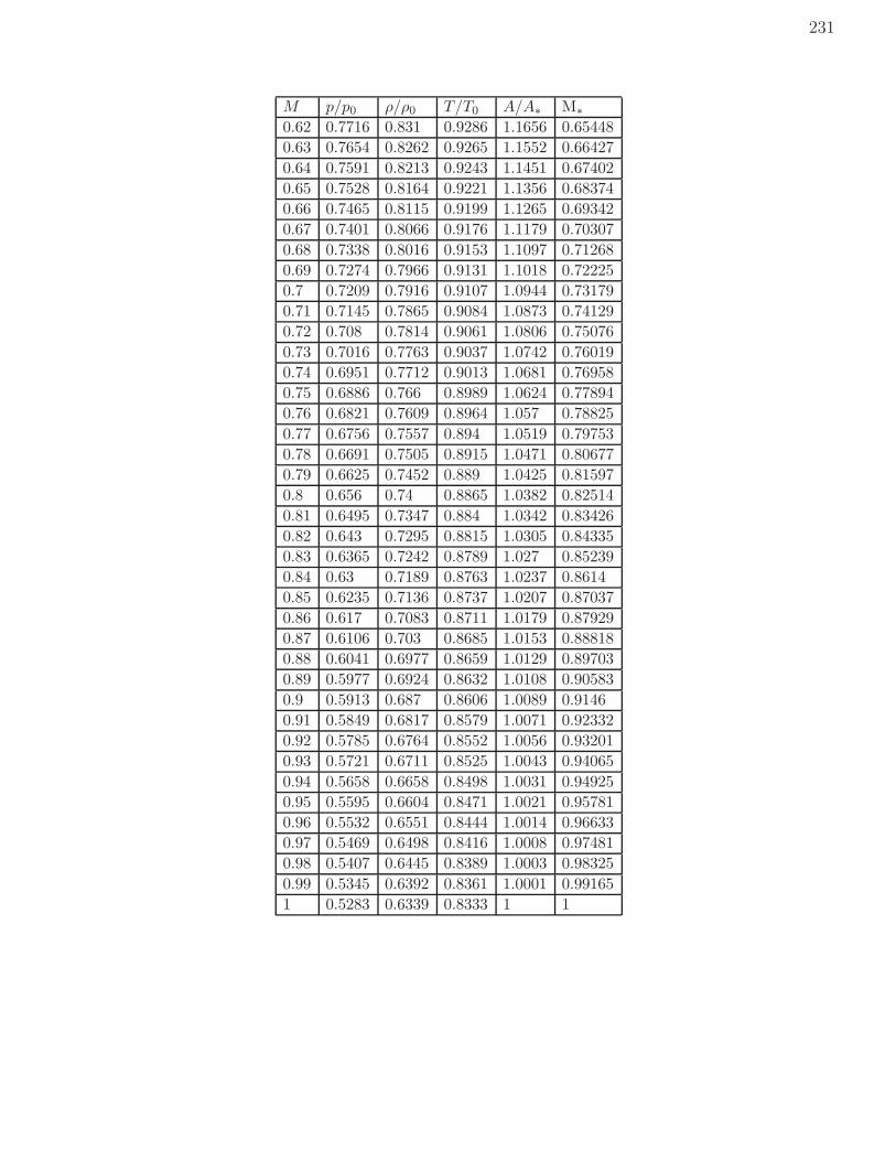
231
M p/p0 ρ/ρ0 T/T0 A/A∗ M∗
0.62 0.7716 0.831 0.9286 1.1656 0.65448
0.63 0.7654 0.8262 0.9265 1.1552 0.66427
0.64 0.7591 0.8213 0.9243 1.1451 0.67402
0.65 0.7528 0.8164 0.9221 1.1356 0.68374
0.66 0.7465 0.8115 0.9199 1.1265 0.69342
0.67 0.7401 0.8066 0.9176 1.1179 0.70307
0.68 0.7338 0.8016 0.9153 1.1097 0.71268
0.69 0.7274 0.7966 0.9131 1.1018 0.72225
0.7 0.7209 0.7916 0.9107 1.0944 0.73179
0.71 0.7145 0.7865 0.9084 1.0873 0.74129
0.72 0.708 0.7814 0.9061 1.0806 0.75076
0.73 0.7016 0.7763 0.9037 1.0742 0.76019
0.74 0.6951 0.7712 0.9013 1.0681 0.76958
0.75 0.6886 0.766 0.8989 1.0624 0.77894
0.76 0.6821 0.7609 0.8964 1.057 0.78825
0.77 0.6756 0.7557 0.894 1.0519 0.79753
0.78 0.6691 0.7505 0.8915 1.0471 0.80677
0.79 0.6625 0.7452 0.889 1.0425 0.81597
0.8 0.656 0.74 0.8865 1.0382 0.82514
0.81 0.6495 0.7347 0.884 1.0342 0.83426
0.82 0.643 0.7295 0.8815 1.0305 0.84335
0.83 0.6365 0.7242 0.8789 1.027 0.85239
0.84 0.63 0.7189 0.8763 1.0237 0.8614
0.85 0.6235 0.7136 0.8737 1.0207 0.87037
0.86 0.617 0.7083 0.8711 1.0179 0.87929
0.87 0.6106 0.703 0.8685 1.0153 0.88818
0.88 0.6041 0.6977 0.8659 1.0129 0.89703
0.89 0.5977 0.6924 0.8632 1.0108 0.90583
0.9 0.5913 0.687 0.8606 1.0089 0.9146
0.91 0.5849 0.6817 0.8579 1.0071 0.92332
0.92 0.5785 0.6764 0.8552 1.0056 0.93201
0.93 0.5721 0.6711 0.8525 1.0043 0.94065
0.94 0.5658 0.6658 0.8498 1.0031 0.94925
0.95 0.5595 0.6604 0.8471 1.0021 0.95781
0.96 0.5532 0.6551 0.8444 1.0014 0.96633
0.97 0.5469 0.6498 0.8416 1.0008 0.97481
0.98 0.5407 0.6445 0.8389 1.0003 0.98325
0.99 0.5345 0.6392 0.8361 1.0001 0.99165
1 0.5283 0.6339 0.8333 1 1

232 Appendix E. Application table for subsonic compressible flows

Appendix F
Application table for supersonic flows,shock waves and rarefaction waves
This chapter contains useful quantitative values concerning compressible flows in the supersonic regime(see Chapter 11), shock waves as well as rarefaction waves. All the results are only valid for a value ofthe heat capacity ratio γ = 1.4! Please note that the variable ν (sixth column), needed to compute therarefaction waves, is not yet discussed in the current version of this document.
M p/p0 ρ/ρ0 T/T0 A/A∗ ν µ M2 p2/p1 ρ2/ρ1 T2/T1 p02/p011 0.5283 0.6339 0.8333 1 0 90 1 1 1 1 1
1.01 0.5221 0.6287 0.8306 1 0.044725 81.93 0.9901 1.023 1.017 1.007 1
1.02 0.516 0.6234 0.8278 1 0.12569 78.64 0.9805 1.047 1.033 1.013 1
1.03 0.5099 0.6181 0.825 1.001 0.22943 76.14 0.9712 1.071 1.05 1.02 1
1.04 0.5039 0.6129 0.8222 1.001 0.35098 74.06 0.962 1.095 1.067 1.026 0.99991.05 0.4979 0.6077 0.8193 1.002 0.48741 72.25 0.9531 1.12 1.084 1.033 0.99991.06 0.4919 0.6024 0.8165 1.003 0.63669 70.63 0.9444 1.144 1.101 1.039 0.99981.07 0.486 0.5972 0.8137 1.004 0.79729 69.16 0.936 1.169 1.118 1.046 0.99961.08 0.48 0.592 0.8108 1.005 0.96804 67.81 0.9277 1.194 1.135 1.052 0.99941.09 0.4742 0.5869 0.808 1.006 1.1479 66.55 0.9196 1.219 1.152 1.059 0.99921.1 0.4684 0.5817 0.8052 1.008 1.3362 65.38 0.9118 1.245 1.169 1.065 0.99891.11 0.4626 0.5766 0.8023 1.01 1.5321 64.28 0.9041 1.271 1.186 1.071 0.99861.12 0.4568 0.5714 0.7994 1.011 1.735 63.23 0.8966 1.297 1.203 1.078 0.99821.13 0.4511 0.5663 0.7966 1.013 1.9445 62.25 0.8892 1.323 1.221 1.084 0.99781.14 0.4455 0.5612 0.7937 1.015 2.16 61.31 0.882 1.35 1.238 1.09 0.99731.15 0.4398 0.5562 0.7908 1.017 2.381 60.41 0.875 1.376 1.255 1.097 0.99671.16 0.4343 0.5511 0.7879 1.02 2.6073 59.55 0.8682 1.403 1.272 1.103 0.99611.17 0.4287 0.5461 0.7851 1.022 2.8385 58.73 0.8615 1.43 1.29 1.109 0.99531.18 0.4232 0.5411 0.7822 1.025 3.0743 57.94 0.8549 1.458 1.307 1.115 0.99461.19 0.4178 0.5361 0.7793 1.028 3.3142 57.18 0.8485 1.485 1.324 1.122 0.99371.2 0.4124 0.5311 0.7764 1.03 3.5582 56.44 0.8422 1.513 1.342 1.128 0.99281.21 0.407 0.5262 0.7735 1.033 3.806 55.74 0.836 1.541 1.359 1.134 0.99181.22 0.4017 0.5213 0.7706 1.037 4.0572 55.05 0.83 1.57 1.376 1.141 0.99071.23 0.3964 0.5164 0.7677 1.04 4.3117 54.39 0.8241 1.598 1.394 1.147 0.98961.24 0.3912 0.5115 0.7648 1.043 4.5694 53.75 0.8183 1.627 1.411 1.153 0.98841.25 0.3861 0.5067 0.7619 1.047 4.8299 53.13 0.8126 1.656 1.429 1.159 0.98711.26 0.3809 0.5019 0.759 1.05 5.0931 52.53 0.8071 1.686 1.446 1.166 0.98571.27 0.3759 0.4971 0.7561 1.054 5.359 51.94 0.8016 1.715 1.463 1.172 0.98421.28 0.3708 0.4923 0.7532 1.058 5.6272 51.38 0.7963 1.745 1.481 1.178 0.98271.29 0.3658 0.4876 0.7503 1.062 5.8977 50.82 0.7911 1.775 1.498 1.185 0.98111.3 0.3609 0.4829 0.7474 1.066 6.1703 50.28 0.786 1.805 1.516 1.191 0.97941.31 0.356 0.4782 0.7445 1.071 6.4449 49.76 0.7809 1.835 1.533 1.197 0.9776
233

234 Appendix F. Application table for supersonic flows, shock waves and rarefaction waves
M p/p0 ρ/ρ0 T/T0 A/A∗ ν µ M2 p2/p1 ρ2/ρ1 T2/T1 p02/p011.32 0.3512 0.4736 0.7416 1.075 6.7213 49.25 0.776 1.866 1.551 1.204 0.97581.33 0.3464 0.469 0.7387 1.08 6.9995 48.75 0.7712 1.897 1.568 1.21 0.97381.34 0.3417 0.4644 0.7358 1.084 7.2794 48.27 0.7664 1.928 1.585 1.216 0.97181.35 0.337 0.4598 0.7329 1.089 7.5607 47.79 0.7618 1.96 1.603 1.223 0.96971.36 0.3323 0.4553 0.73 1.094 7.8435 47.33 0.7572 1.991 1.62 1.229 0.96761.37 0.3277 0.4508 0.7271 1.099 8.1276 46.88 0.7527 2.023 1.638 1.235 0.96531.38 0.3232 0.4463 0.7242 1.104 8.413 46.44 0.7483 2.055 1.655 1.242 0.9631.39 0.3187 0.4418 0.7213 1.109 8.6995 46.01 0.744 2.087 1.672 1.248 0.96071.4 0.3142 0.4374 0.7184 1.115 8.987 45.58 0.7397 2.12 1.69 1.255 0.95821.41 0.3098 0.433 0.7155 1.12 9.2756 45.17 0.7355 2.153 1.707 1.261 0.95571.42 0.3055 0.4287 0.7126 1.126 9.565 44.77 0.7314 2.186 1.724 1.268 0.95311.43 0.3012 0.4244 0.7097 1.132 9.8553 44.37 0.7274 2.219 1.742 1.274 0.95041.44 0.2969 0.4201 0.7069 1.138 10.146 43.98 0.7235 2.253 1.759 1.281 0.94761.45 0.2927 0.4158 0.704 1.144 10.438 43.6 0.7196 2.286 1.776 1.287 0.94481.46 0.2886 0.4116 0.7011 1.15 10.731 43.23 0.7157 2.32 1.793 1.294 0.9421.47 0.2845 0.4074 0.6982 1.156 11.023 42.86 0.712 2.354 1.811 1.3 0.9391.48 0.2804 0.4032 0.6954 1.163 11.317 42.51 0.7083 2.389 1.828 1.307 0.9361.49 0.2764 0.3991 0.6925 1.169 11.611 42.16 0.7047 2.423 1.845 1.314 0.93291.5 0.2724 0.395 0.6897 1.176 11.905 41.81 0.7011 2.458 1.862 1.32 0.92981.51 0.2685 0.3909 0.6868 1.183 12.2 41.47 0.6976 2.493 1.879 1.327 0.92661.52 0.2646 0.3869 0.684 1.19 12.495 41.14 0.6941 2.529 1.896 1.334 0.92331.53 0.2608 0.3829 0.6811 1.197 12.79 40.81 0.6907 2.564 1.913 1.34 0.921.54 0.257 0.3789 0.6783 1.204 13.086 40.49 0.6874 2.6 1.93 1.347 0.91661.55 0.2533 0.375 0.6754 1.212 13.381 40.18 0.6841 2.636 1.947 1.354 0.91321.56 0.2496 0.371 0.6726 1.219 13.677 39.87 0.6809 2.673 1.964 1.361 0.90971.57 0.2459 0.3672 0.6698 1.227 13.973 39.56 0.6777 2.709 1.981 1.367 0.90621.58 0.2423 0.3633 0.667 1.234 14.269 39.27 0.6746 2.746 1.998 1.374 0.90261.59 0.2388 0.3595 0.6642 1.242 14.565 38.97 0.6715 2.783 2.015 1.381 0.89891.6 0.2353 0.3557 0.6614 1.25 14.86 38.68 0.6684 2.82 2.032 1.388 0.89521.61 0.2318 0.352 0.6586 1.258 15.156 38.4 0.6655 2.857 2.049 1.395 0.89151.62 0.2284 0.3483 0.6558 1.267 15.452 38.12 0.6625 2.895 2.065 1.402 0.88771.63 0.225 0.3446 0.653 1.275 15.747 37.84 0.6596 2.933 2.082 1.409 0.88381.64 0.2217 0.3409 0.6502 1.284 16.043 37.57 0.6568 2.971 2.099 1.416 0.87991.65 0.2184 0.3373 0.6475 1.292 16.338 37.31 0.654 3.01 2.115 1.423 0.8761.66 0.2151 0.3337 0.6447 1.301 16.633 37.04 0.6512 3.048 2.132 1.43 0.8721.67 0.2119 0.3302 0.6419 1.31 16.928 36.78 0.6485 3.087 2.148 1.437 0.8681.68 0.2088 0.3266 0.6392 1.319 17.222 36.53 0.6458 3.126 2.165 1.444 0.86391.69 0.2057 0.3232 0.6364 1.328 17.516 36.28 0.6431 3.165 2.181 1.451 0.85991.7 0.2026 0.3197 0.6337 1.338 17.81 36.03 0.6405 3.205 2.198 1.458 0.85571.71 0.1996 0.3163 0.631 1.347 18.103 35.79 0.638 3.245 2.214 1.466 0.85161.72 0.1966 0.3129 0.6283 1.357 18.396 35.55 0.6355 3.285 2.23 1.473 0.84741.73 0.1936 0.3095 0.6256 1.367 18.689 35.31 0.633 3.325 2.247 1.48 0.84311.74 0.1907 0.3062 0.6229 1.376 18.981 35.08 0.6305 3.366 2.263 1.487 0.83891.75 0.1878 0.3029 0.6202 1.386 19.273 34.85 0.6281 3.406 2.279 1.495 0.83461.76 0.185 0.2996 0.6175 1.397 19.565 34.62 0.6257 3.447 2.295 1.502 0.83021.77 0.1822 0.2964 0.6148 1.407 19.855 34.4 0.6234 3.488 2.311 1.509 0.82591.78 0.1794 0.2931 0.6121 1.418 20.146 34.18 0.621 3.53 2.327 1.517 0.82151.79 0.1767 0.29 0.6095 1.428 20.436 33.96 0.6188 3.571 2.343 1.524 0.81711.8 0.174 0.2868 0.6068 1.439 20.725 33.75 0.6165 3.613 2.359 1.532 0.8127

235
M p/p0 ρ/ρ0 T/T0 A/A∗ ν µ M2 p2/p1 ρ2/ρ1 T2/T1 p02/p011.81 0.1714 0.2837 0.6041 1.45 21.014 33.54 0.6143 3.655 2.375 1.539 0.80821.82 0.1688 0.2806 0.6015 1.461 21.302 33.33 0.6121 3.698 2.391 1.547 0.80381.83 0.1662 0.2776 0.5989 1.472 21.59 33.12 0.6099 3.74 2.407 1.554 0.79931.84 0.1637 0.2745 0.5963 1.484 21.877 32.92 0.6078 3.783 2.422 1.562 0.79481.85 0.1612 0.2715 0.5936 1.495 22.163 32.72 0.6057 3.826 2.438 1.569 0.79021.86 0.1587 0.2686 0.591 1.507 22.449 32.52 0.6036 3.87 2.454 1.577 0.78571.87 0.1563 0.2656 0.5884 1.519 22.734 32.33 0.6016 3.913 2.469 1.585 0.78111.88 0.1539 0.2627 0.5859 1.531 23.019 32.13 0.5996 3.957 2.485 1.592 0.77651.89 0.1516 0.2598 0.5833 1.543 23.303 31.94 0.5976 4.001 2.5 1.6 0.7721.9 0.1492 0.257 0.5807 1.555 23.586 31.76 0.5956 4.045 2.516 1.608 0.76741.91 0.147 0.2542 0.5782 1.568 23.869 31.57 0.5937 4.089 2.531 1.616 0.76271.92 0.1447 0.2514 0.5756 1.58 24.151 31.39 0.5918 4.134 2.546 1.624 0.75811.93 0.1425 0.2486 0.5731 1.593 24.432 31.21 0.5899 4.179 2.562 1.631 0.75351.94 0.1403 0.2459 0.5705 1.606 24.712 31.03 0.588 4.224 2.577 1.639 0.74881.95 0.1381 0.2432 0.568 1.619 24.992 30.85 0.5862 4.27 2.592 1.647 0.74421.96 0.136 0.2405 0.5655 1.633 25.271 30.68 0.5844 4.315 2.607 1.655 0.73951.97 0.1339 0.2378 0.563 1.646 25.549 30.51 0.5826 4.361 2.622 1.663 0.73491.98 0.1318 0.2352 0.5605 1.66 25.827 30.33 0.5808 4.407 2.637 1.671 0.73021.99 0.1298 0.2326 0.558 1.674 26.104 30.17 0.5791 4.453 2.652 1.679 0.72552 0.1278 0.23 0.5556 1.688 26.38 30 0.5774 4.5 2.667 1.687 0.72092.01 0.1258 0.2275 0.5531 1.702 26.655 29.84 0.5757 4.547 2.681 1.696 0.71622.02 0.1239 0.225 0.5506 1.716 26.93 29.67 0.574 4.594 2.696 1.704 0.71152.03 0.122 0.2225 0.5482 1.73 27.203 29.51 0.5723 4.641 2.711 1.712 0.70692.04 0.1201 0.22 0.5458 1.745 27.476 29.35 0.5707 4.689 2.725 1.72 0.70222.05 0.1182 0.2176 0.5433 1.76 27.748 29.2 0.5691 4.736 2.74 1.729 0.69752.06 0.1164 0.2152 0.5409 1.775 28.02 29.04 0.5675 4.784 2.755 1.737 0.69282.07 0.1146 0.2128 0.5385 1.79 28.29 28.89 0.5659 4.832 2.769 1.745 0.68822.08 0.1128 0.2104 0.5361 1.806 28.56 28.74 0.5643 4.881 2.783 1.754 0.68352.09 0.1111 0.2081 0.5337 1.821 28.829 28.59 0.5628 4.929 2.798 1.762 0.67892.1 0.1094 0.2058 0.5313 1.837 29.097 28.44 0.5613 4.978 2.812 1.77 0.67422.11 0.1077 0.2035 0.529 1.853 29.364 28.29 0.5598 5.027 2.826 1.779 0.66962.12 0.106 0.2013 0.5266 1.869 29.631 28.14 0.5583 5.077 2.84 1.787 0.66492.13 0.1043 0.199 0.5243 1.885 29.896 28 0.5568 5.126 2.854 1.796 0.66032.14 0.1027 0.1968 0.5219 1.902 30.161 27.86 0.5554 5.176 2.868 1.805 0.65572.15 0.1011 0.1946 0.5196 1.919 30.425 27.72 0.554 5.226 2.882 1.813 0.65112.16 0.09956 0.1925 0.5173 1.935 30.688 27.58 0.5525 5.277 2.896 1.822 0.64642.17 0.09802 0.1903 0.515 1.953 30.951 27.44 0.5511 5.327 2.91 1.831 0.64192.18 0.09649 0.1882 0.5127 1.97 31.212 27.3 0.5498 5.378 2.924 1.839 0.63732.19 0.095 0.1861 0.5104 1.987 31.473 27.17 0.5484 5.429 2.938 1.848 0.63272.2 0.09352 0.1841 0.5081 2.005 31.732 27.04 0.5471 5.48 2.951 1.857 0.62812.21 0.09207 0.182 0.5059 2.023 31.991 26.9 0.5457 5.531 2.965 1.866 0.62362.22 0.09064 0.18 0.5036 2.041 32.249 26.77 0.5444 5.583 2.978 1.875 0.61912.23 0.08923 0.178 0.5014 2.059 32.507 26.64 0.5431 5.635 2.992 1.883 0.61452.24 0.08785 0.176 0.4991 2.078 32.763 26.51 0.5418 5.687 3.005 1.892 0.612.25 0.08648 0.174 0.4969 2.096 33.018 26.39 0.5406 5.74 3.019 1.901 0.60552.26 0.08514 0.1721 0.4947 2.115 33.273 26.26 0.5393 5.792 3.032 1.91 0.60112.27 0.08382 0.1702 0.4925 2.134 33.527 26.14 0.5381 5.845 3.045 1.919 0.59662.28 0.08251 0.1683 0.4903 2.154 33.78 26.01 0.5368 5.898 3.058 1.929 0.59212.29 0.08123 0.1664 0.4881 2.173 34.032 25.89 0.5356 5.951 3.071 1.938 0.5877

236 Appendix F. Application table for supersonic flows, shock waves and rarefaction waves
M p/p0 ρ/ρ0 T/T0 A/A∗ ν µ M2 p2/p1 ρ2/ρ1 T2/T1 p02/p012.3 0.07997 0.1646 0.4859 2.193 34.283 25.77 0.5344 6.005 3.085 1.947 0.58332.31 0.07873 0.1628 0.4837 2.213 34.533 25.65 0.5332 6.059 3.098 1.956 0.57892.32 0.07751 0.1609 0.4816 2.233 34.782 25.53 0.5321 6.113 3.11 1.965 0.57452.33 0.07631 0.1592 0.4794 2.254 35.031 25.42 0.5309 6.167 3.123 1.974 0.57022.34 0.07512 0.1574 0.4773 2.274 35.279 25.3 0.5297 6.222 3.136 1.984 0.56582.35 0.07396 0.1556 0.4752 2.295 35.526 25.18 0.5286 6.276 3.149 1.993 0.56152.36 0.07281 0.1539 0.4731 2.316 35.771 25.07 0.5275 6.331 3.162 2.002 0.55722.37 0.07168 0.1522 0.4709 2.338 36.017 24.96 0.5264 6.386 3.174 2.012 0.55292.38 0.07057 0.1505 0.4688 2.359 36.261 24.85 0.5253 6.442 3.187 2.021 0.54862.39 0.06948 0.1488 0.4668 2.381 36.504 24.73 0.5242 6.497 3.199 2.031 0.54442.4 0.0684 0.1472 0.4647 2.403 36.747 24.62 0.5231 6.553 3.212 2.04 0.54012.41 0.06734 0.1456 0.4626 2.425 36.988 24.52 0.5221 6.609 3.224 2.05 0.53592.42 0.0663 0.1439 0.4606 2.448 37.229 24.41 0.521 6.666 3.237 2.059 0.53172.43 0.06527 0.1424 0.4585 2.471 37.469 24.3 0.52 6.722 3.249 2.069 0.52762.44 0.06426 0.1408 0.4565 2.494 37.708 24.19 0.5189 6.779 3.261 2.079 0.52342.45 0.06327 0.1392 0.4544 2.517 37.946 24.09 0.5179 6.836 3.273 2.088 0.51932.46 0.06229 0.1377 0.4524 2.54 38.183 23.99 0.5169 6.894 3.285 2.098 0.51522.47 0.06133 0.1362 0.4504 2.564 38.42 23.88 0.5159 6.951 3.298 2.108 0.51112.48 0.06038 0.1346 0.4484 2.588 38.655 23.78 0.5149 7.009 3.31 2.118 0.50712.49 0.05945 0.1332 0.4464 2.612 38.89 23.68 0.514 7.067 3.321 2.128 0.5032.5 0.05853 0.1317 0.4444 2.637 39.124 23.58 0.513 7.125 3.333 2.138 0.4992.51 0.05762 0.1302 0.4425 2.661 39.357 23.48 0.512 7.183 3.345 2.147 0.4952.52 0.05674 0.1288 0.4405 2.686 39.589 23.38 0.5111 7.242 3.357 2.157 0.49112.53 0.05586 0.1274 0.4386 2.712 39.82 23.28 0.5102 7.301 3.369 2.167 0.48712.54 0.055 0.126 0.4366 2.737 40.05 23.18 0.5092 7.36 3.38 2.177 0.48322.55 0.05415 0.1246 0.4347 2.763 40.28 23.09 0.5083 7.42 3.392 2.187 0.47932.56 0.05332 0.1232 0.4328 2.789 40.508 22.99 0.5074 7.479 3.403 2.198 0.47542.57 0.0525 0.1218 0.4309 2.815 40.736 22.9 0.5065 7.539 3.415 2.208 0.47152.58 0.05169 0.1205 0.4289 2.842 40.963 22.81 0.5056 7.599 3.426 2.218 0.46772.59 0.0509 0.1192 0.4271 2.869 41.189 22.71 0.5047 7.659 3.438 2.228 0.46392.6 0.05012 0.1179 0.4252 2.896 41.415 22.62 0.5039 7.72 3.449 2.238 0.46012.61 0.04935 0.1166 0.4233 2.923 41.639 22.53 0.503 7.781 3.46 2.249 0.45642.62 0.04859 0.1153 0.4214 2.951 41.863 22.44 0.5022 7.842 3.471 2.259 0.45262.63 0.04784 0.114 0.4196 2.979 42.086 22.35 0.5013 7.903 3.483 2.269 0.44892.64 0.04711 0.1128 0.4177 3.007 42.307 22.26 0.5005 7.965 3.494 2.28 0.44522.65 0.04639 0.1115 0.4159 3.036 42.529 22.17 0.4996 8.026 3.505 2.29 0.44162.66 0.04568 0.1103 0.4141 3.065 42.749 22.08 0.4988 8.088 3.516 2.301 0.43792.67 0.04498 0.1091 0.4122 3.094 42.968 22 0.498 8.15 3.527 2.311 0.43432.68 0.04429 0.1079 0.4104 3.123 43.187 21.91 0.4972 8.213 3.537 2.322 0.43072.69 0.04362 0.1067 0.4086 3.153 43.405 21.82 0.4964 8.275 3.548 2.332 0.42712.7 0.04295 0.1056 0.4068 3.183 43.621 21.74 0.4956 8.338 3.559 2.343 0.42362.71 0.04229 0.1044 0.4051 3.213 43.838 21.65 0.4949 8.401 3.57 2.354 0.42012.72 0.04165 0.1033 0.4033 3.244 44.053 21.57 0.4941 8.465 3.58 2.364 0.41662.73 0.04102 0.1022 0.4015 3.275 44.267 21.49 0.4933 8.528 3.591 2.375 0.41312.74 0.04039 0.101 0.3998 3.306 44.481 21.41 0.4926 8.592 3.601 2.386 0.40972.75 0.03978 0.09994 0.398 3.338 44.694 21.32 0.4918 8.656 3.612 2.397 0.40622.76 0.03917 0.09885 0.3963 3.37 44.906 21.24 0.4911 8.721 3.622 2.407 0.40282.77 0.03858 0.09778 0.3945 3.402 45.117 21.16 0.4903 8.785 3.633 2.418 0.39942.78 0.03799 0.09671 0.3928 3.434 45.327 21.08 0.4896 8.85 3.643 2.429 0.3961

237
M p/p0 ρ/ρ0 T/T0 A/A∗ ν µ M2 p2/p1 ρ2/ρ1 T2/T1 p02/p012.79 0.03742 0.09566 0.3911 3.467 45.537 21 0.4889 8.915 3.653 2.44 0.39282.8 0.03685 0.09463 0.3894 3.5 45.746 20.92 0.4882 8.98 3.664 2.451 0.38952.81 0.03629 0.0936 0.3877 3.534 45.954 20.85 0.4875 9.045 3.674 2.462 0.38622.82 0.03574 0.09259 0.386 3.567 46.161 20.77 0.4868 9.111 3.684 2.473 0.38292.83 0.0352 0.09158 0.3844 3.601 46.368 20.69 0.4861 9.177 3.694 2.484 0.37972.84 0.03467 0.09059 0.3827 3.636 46.573 20.62 0.4854 9.243 3.704 2.496 0.37652.85 0.03415 0.08962 0.381 3.671 46.778 20.54 0.4847 9.31 3.714 2.507 0.37332.86 0.03363 0.08865 0.3794 3.706 46.982 20.47 0.484 9.376 3.724 2.518 0.37012.87 0.03312 0.08769 0.3777 3.741 47.185 20.39 0.4833 9.443 3.734 2.529 0.3672.88 0.03263 0.08675 0.3761 3.777 47.388 20.32 0.4827 9.51 3.743 2.54 0.36392.89 0.03213 0.08581 0.3745 3.813 47.589 20.24 0.482 9.577 3.753 2.552 0.36082.9 0.03165 0.08489 0.3729 3.85 47.79 20.17 0.4814 9.645 3.763 2.563 0.35772.91 0.03118 0.08398 0.3712 3.887 47.99 20.1 0.4807 9.713 3.773 2.575 0.35472.92 0.03071 0.08307 0.3696 3.924 48.19 20.03 0.4801 9.781 3.782 2.586 0.35172.93 0.03025 0.08218 0.3681 3.961 48.388 19.96 0.4795 9.849 3.792 2.598 0.34872.94 0.0298 0.0813 0.3665 3.999 48.586 19.89 0.4788 9.918 3.801 2.609 0.34572.95 0.02935 0.08043 0.3649 4.038 48.783 19.81 0.4782 9.986 3.811 2.621 0.34282.96 0.02891 0.07957 0.3633 4.076 48.98 19.75 0.4776 10.06 3.82 2.632 0.33982.97 0.02848 0.07872 0.3618 4.115 49.175 19.68 0.477 10.12 3.829 2.644 0.33692.98 0.02805 0.07788 0.3602 4.155 49.37 19.61 0.4764 10.19 3.839 2.656 0.3342.99 0.02764 0.07705 0.3587 4.194 49.564 19.54 0.4758 10.26 3.848 2.667 0.33123 0.02722 0.07623 0.3571 4.235 49.757 19.47 0.4752 10.33 3.857 2.679 0.32833.01 0.02682 0.07541 0.3556 4.275 49.95 19.4 0.4746 10.4 3.866 2.691 0.32553.02 0.02642 0.07461 0.3541 4.316 50.142 19.34 0.474 10.47 3.875 2.703 0.32273.03 0.02603 0.07382 0.3526 4.357 50.333 19.27 0.4734 10.54 3.884 2.714 0.323.04 0.02564 0.07303 0.3511 4.399 50.523 19.2 0.4729 10.62 3.893 2.726 0.31723.05 0.02526 0.07226 0.3496 4.441 50.713 19.14 0.4723 10.69 3.902 2.738 0.31453.06 0.02489 0.07149 0.3481 4.483 50.902 19.07 0.4717 10.76 3.911 2.75 0.31183.07 0.02452 0.07074 0.3466 4.526 51.09 19.01 0.4712 10.83 3.92 2.762 0.30913.08 0.02416 0.06999 0.3452 4.57 51.277 18.95 0.4706 10.9 3.929 2.774 0.30653.09 0.0238 0.06925 0.3437 4.613 51.464 18.88 0.4701 10.97 3.938 2.786 0.30383.1 0.02345 0.06852 0.3422 4.657 51.65 18.82 0.4695 11.05 3.947 2.799 0.30123.11 0.0231 0.06779 0.3408 4.702 51.835 18.76 0.469 11.12 3.955 2.811 0.29863.12 0.02276 0.06708 0.3393 4.747 52.02 18.69 0.4685 11.19 3.964 2.823 0.2963.13 0.02243 0.06637 0.3379 4.792 52.203 18.63 0.4679 11.26 3.973 2.835 0.29353.14 0.0221 0.06568 0.3365 4.838 52.386 18.57 0.4674 11.34 3.981 2.848 0.2913.15 0.02177 0.06499 0.3351 4.884 52.569 18.51 0.4669 11.41 3.99 2.86 0.28853.16 0.02146 0.0643 0.3337 4.93 52.751 18.45 0.4664 11.48 3.998 2.872 0.2863.17 0.02114 0.06363 0.3323 4.977 52.932 18.39 0.4659 11.56 4.006 2.885 0.28353.18 0.02083 0.06296 0.3309 5.025 53.112 18.33 0.4654 11.63 4.015 2.897 0.28113.19 0.02053 0.06231 0.3295 5.073 53.291 18.27 0.4648 11.71 4.023 2.909 0.27863.2 0.02023 0.06165 0.3281 5.121 53.47 18.21 0.4643 11.78 4.031 2.922 0.27623.21 0.01993 0.06101 0.3267 5.17 53.649 18.15 0.4639 11.85 4.04 2.935 0.27383.22 0.01964 0.06037 0.3253 5.219 53.826 18.09 0.4634 11.93 4.048 2.947 0.27153.23 0.01936 0.05975 0.324 5.268 54.003 18.03 0.4629 12.01 4.056 2.96 0.26913.24 0.01908 0.05912 0.3226 5.319 54.179 17.98 0.4624 12.08 4.064 2.972 0.26683.25 0.0188 0.05851 0.3213 5.369 54.355 17.92 0.4619 12.16 4.072 2.985 0.26453.26 0.01853 0.0579 0.3199 5.42 54.529 17.86 0.4614 12.23 4.08 2.998 0.26223.27 0.01826 0.0573 0.3186 5.472 54.704 17.81 0.461 12.31 4.088 3.011 0.26

238 Appendix F. Application table for supersonic flows, shock waves and rarefaction waves
M p/p0 ρ/ρ0 T/T0 A/A∗ ν µ M2 p2/p1 ρ2/ρ1 T2/T1 p02/p013.28 0.01799 0.05671 0.3173 5.523 54.877 17.75 0.4605 12.38 4.096 3.023 0.25773.29 0.01773 0.05612 0.316 5.576 55.05 17.7 0.46 12.46 4.104 3.036 0.25553.3 0.01748 0.05554 0.3147 5.629 55.222 17.64 0.4596 12.54 4.112 3.049 0.25333.31 0.01722 0.05497 0.3134 5.682 55.393 17.58 0.4591 12.62 4.12 3.062 0.25113.32 0.01698 0.0544 0.3121 5.736 55.564 17.53 0.4587 12.69 4.128 3.075 0.24893.33 0.01673 0.05384 0.3108 5.79 55.734 17.48 0.4582 12.77 4.135 3.088 0.24683.34 0.01649 0.05329 0.3095 5.845 55.904 17.42 0.4578 12.85 4.143 3.101 0.24463.35 0.01625 0.05274 0.3082 5.9 56.073 17.37 0.4573 12.93 4.151 3.114 0.24253.36 0.01602 0.0522 0.3069 5.956 56.241 17.31 0.4569 13 4.158 3.127 0.24043.37 0.01579 0.05166 0.3057 6.012 56.409 17.26 0.4565 13.08 4.166 3.141 0.23833.38 0.01557 0.05113 0.3044 6.069 56.576 17.21 0.456 13.16 4.173 3.154 0.23633.39 0.01534 0.05061 0.3032 6.126 56.742 17.16 0.4556 13.24 4.181 3.167 0.23423.4 0.01512 0.05009 0.3019 6.184 56.908 17.1 0.4552 13.32 4.188 3.18 0.23223.41 0.01491 0.04958 0.3007 6.242 57.073 17.05 0.4548 13.4 4.196 3.194 0.23023.42 0.0147 0.04908 0.2995 6.301 57.237 17 0.4544 13.48 4.203 3.207 0.22823.43 0.01449 0.04858 0.2982 6.36 57.401 16.95 0.454 13.56 4.211 3.22 0.22633.44 0.01428 0.04808 0.297 6.42 57.564 16.9 0.4535 13.64 4.218 3.234 0.22433.45 0.01408 0.04759 0.2958 6.48 57.726 16.85 0.4531 13.72 4.225 3.247 0.22243.46 0.01388 0.04711 0.2946 6.541 57.888 16.8 0.4527 13.8 4.232 3.261 0.22053.47 0.01368 0.04663 0.2934 6.602 58.05 16.75 0.4523 13.88 4.24 3.274 0.21863.48 0.01349 0.04616 0.2922 6.664 58.21 16.7 0.4519 13.96 4.247 3.288 0.21673.49 0.0133 0.04569 0.291 6.727 58.37 16.65 0.4515 14.04 4.254 3.301 0.21483.5 0.01311 0.04523 0.2899 6.79 58.53 16.6 0.4512 14.12 4.261 3.315 0.21293.51 0.01293 0.04478 0.2887 6.853 58.689 16.55 0.4508 14.21 4.268 3.329 0.21113.52 0.01274 0.04433 0.2875 6.917 58.847 16.5 0.4504 14.29 4.275 3.342 0.20933.53 0.01256 0.04388 0.2864 6.982 59.005 16.46 0.45 14.37 4.282 3.356 0.20753.54 0.01239 0.04344 0.2852 7.047 59.162 16.41 0.4496 14.45 4.289 3.37 0.20573.55 0.01221 0.043 0.2841 7.113 59.318 16.36 0.4492 14.54 4.296 3.384 0.20393.56 0.01204 0.04257 0.2829 7.179 59.474 16.31 0.4489 14.62 4.303 3.398 0.20223.57 0.01188 0.04214 0.2818 7.246 59.629 16.27 0.4485 14.7 4.309 3.412 0.20043.58 0.01171 0.04172 0.2806 7.313 59.784 16.22 0.4481 14.79 4.316 3.426 0.19873.59 0.01155 0.04131 0.2795 7.381 59.938 16.17 0.4478 14.87 4.323 3.44 0.1973.6 0.01138 0.04089 0.2784 7.45 60.091 16.13 0.4474 14.95 4.33 3.454 0.19533.61 0.01123 0.04049 0.2773 7.519 60.244 16.08 0.4471 15.04 4.336 3.468 0.19363.62 0.01107 0.04008 0.2762 7.589 60.397 16.04 0.4467 15.12 4.343 3.482 0.1923.63 0.01092 0.03968 0.2751 7.659 60.549 15.99 0.4463 15.21 4.35 3.496 0.19033.64 0.01076 0.03929 0.274 7.73 60.7 15.95 0.446 15.29 4.356 3.51 0.18873.65 0.01062 0.0389 0.2729 7.802 60.85 15.9 0.4456 15.38 4.363 3.525 0.18713.66 0.01047 0.03852 0.2718 7.874 61.001 15.86 0.4453 15.46 4.369 3.539 0.18553.67 0.01032 0.03813 0.2707 7.947 61.15 15.81 0.445 15.55 4.376 3.553 0.18393.68 0.01018 0.03776 0.2697 8.02 61.299 15.77 0.4446 15.63 4.382 3.567 0.18233.69 0.01004 0.03739 0.2686 8.094 61.447 15.72 0.4443 15.72 4.388 3.582 0.18073.7 0.009903 0.03702 0.2675 8.169 61.595 15.68 0.4439 15.81 4.395 3.596 0.17923.71 0.009767 0.03665 0.2665 8.244 61.743 15.64 0.4436 15.89 4.401 3.611 0.17773.72 0.009633 0.03629 0.2654 8.32 61.889 15.59 0.4433 15.98 4.408 3.625 0.17613.73 0.0095 0.03594 0.2644 8.397 62.036 15.55 0.443 16.07 4.414 3.64 0.17463.74 0.00937 0.03558 0.2633 8.474 62.181 15.51 0.4426 16.15 4.42 3.654 0.17313.75 0.009242 0.03524 0.2623 8.552 62.326 15.47 0.4423 16.24 4.426 3.669 0.17173.76 0.009116 0.03489 0.2613 8.63 62.471 15.42 0.442 16.33 4.432 3.684 0.1702

239
M p/p0 ρ/ρ0 T/T0 A/A∗ ν µ M2 p2/p1 ρ2/ρ1 T2/T1 p02/p013.77 0.008991 0.03455 0.2602 8.709 62.615 15.38 0.4417 16.42 4.439 3.698 0.16873.78 0.008869 0.03421 0.2592 8.789 62.758 15.34 0.4414 16.5 4.445 3.713 0.16733.79 0.008748 0.03388 0.2582 8.869 62.901 15.3 0.441 16.59 4.451 3.728 0.16593.8 0.008629 0.03355 0.2572 8.951 63.044 15.26 0.4407 16.68 4.457 3.743 0.16453.81 0.008512 0.03322 0.2562 9.032 63.186 15.22 0.4404 16.77 4.463 3.757 0.16313.82 0.008396 0.0329 0.2552 9.115 63.327 15.18 0.4401 16.86 4.469 3.772 0.16173.83 0.008283 0.03258 0.2542 9.198 63.468 15.14 0.4398 16.95 4.475 3.787 0.16033.84 0.008171 0.03227 0.2532 9.282 63.608 15.09 0.4395 17.04 4.481 3.802 0.15893.85 0.00806 0.03195 0.2522 9.366 63.748 15.05 0.4392 17.13 4.487 3.817 0.15763.86 0.007951 0.03165 0.2513 9.451 63.887 15.01 0.4389 17.22 4.492 3.832 0.15633.87 0.007844 0.03134 0.2503 9.537 64.026 14.98 0.4386 17.31 4.498 3.847 0.15493.88 0.007739 0.03104 0.2493 9.624 64.164 14.94 0.4383 17.4 4.504 3.862 0.15363.89 0.007635 0.03074 0.2484 9.711 64.302 14.9 0.438 17.49 4.51 3.878 0.15233.9 0.007532 0.03044 0.2474 9.799 64.44 14.86 0.4377 17.58 4.516 3.893 0.1513.91 0.007431 0.03015 0.2464 9.888 64.576 14.82 0.4375 17.67 4.521 3.908 0.14973.92 0.007332 0.02986 0.2455 9.977 64.713 14.78 0.4372 17.76 4.527 3.923 0.14853.93 0.007233 0.02958 0.2446 10.07 64.848 14.74 0.4369 17.85 4.533 3.939 0.14723.94 0.007137 0.02929 0.2436 10.16 64.984 14.7 0.4366 17.94 4.538 3.954 0.1463.95 0.007042 0.02902 0.2427 10.25 65.118 14.66 0.4363 18.04 4.544 3.969 0.14483.96 0.006948 0.02874 0.2418 10.34 65.253 14.63 0.436 18.13 4.549 3.985 0.14353.97 0.006855 0.02846 0.2408 10.44 65.386 14.59 0.4358 18.22 4.555 4 0.14233.98 0.006764 0.02819 0.2399 10.53 65.52 14.55 0.4355 18.31 4.56 4.016 0.14113.99 0.006675 0.02793 0.239 10.62 65.652 14.51 0.4352 18.41 4.566 4.031 0.13994 0.006586 0.02766 0.2381 10.72 65.785 14.48 0.435 18.5 4.571 4.047 0.13884.01 0.006499 0.0274 0.2372 10.81 65.917 14.44 0.4347 18.59 4.577 4.062 0.13764.02 0.006413 0.02714 0.2363 10.91 66.048 14.4 0.4344 18.69 4.582 4.078 0.13644.03 0.006328 0.02688 0.2354 11.01 66.179 14.37 0.4342 18.78 4.588 4.094 0.13534.04 0.006245 0.02663 0.2345 11.11 66.309 14.33 0.4339 18.88 4.593 4.11 0.13424.05 0.006163 0.02638 0.2336 11.21 66.439 14.29 0.4336 18.97 4.598 4.125 0.1334.06 0.006082 0.02613 0.2327 11.31 66.569 14.26 0.4334 19.06 4.604 4.141 0.13194.07 0.006002 0.02589 0.2319 11.41 66.698 14.22 0.4331 19.16 4.609 4.157 0.13084.08 0.005923 0.02564 0.231 11.51 66.826 14.19 0.4329 19.25 4.614 4.173 0.12974.09 0.005845 0.0254 0.2301 11.61 66.954 14.15 0.4326 19.35 4.619 4.189 0.12864.1 0.005769 0.02516 0.2293 11.71 67.082 14.12 0.4324 19.44 4.624 4.205 0.12764.11 0.005694 0.02493 0.2284 11.82 67.209 14.08 0.4321 19.54 4.63 4.221 0.12654.12 0.005619 0.0247 0.2275 11.92 67.336 14.05 0.4319 19.64 4.635 4.237 0.12544.13 0.005546 0.02447 0.2267 12.03 67.462 14.01 0.4316 19.73 4.64 4.253 0.12444.14 0.005474 0.02424 0.2258 12.14 67.588 13.98 0.4314 19.83 4.645 4.269 0.12344.15 0.005403 0.02401 0.225 12.24 67.713 13.94 0.4311 19.93 4.65 4.285 0.12234.16 0.005333 0.02379 0.2242 12.35 67.838 13.91 0.4309 20.02 4.655 4.301 0.12134.17 0.005264 0.02357 0.2233 12.46 67.963 13.88 0.4306 20.12 4.66 4.318 0.12034.18 0.005195 0.02335 0.2225 12.57 68.087 13.84 0.4304 20.22 4.665 4.334 0.11934.19 0.005128 0.02313 0.2217 12.68 68.21 13.81 0.4302 20.32 4.67 4.35 0.11834.2 0.005062 0.02292 0.2208 12.79 68.333 13.77 0.4299 20.41 4.675 4.367 0.11734.21 0.004997 0.02271 0.22 12.9 68.456 13.74 0.4297 20.51 4.68 4.383 0.11644.22 0.004932 0.0225 0.2192 13.02 68.578 13.71 0.4295 20.61 4.685 4.399 0.11544.23 0.004869 0.02229 0.2184 13.13 68.7 13.67 0.4292 20.71 4.69 4.416 0.11444.24 0.004806 0.02209 0.2176 13.25 68.821 13.64 0.429 20.81 4.694 4.432 0.11354.25 0.004745 0.02189 0.2168 13.36 68.942 13.61 0.4288 20.91 4.699 4.449 0.1126

240 Appendix F. Application table for supersonic flows, shock waves and rarefaction waves
M p/p0 ρ/ρ0 T/T0 A/A∗ ν µ M2 p2/p1 ρ2/ρ1 T2/T1 p02/p014.26 0.004684 0.02169 0.216 13.48 69.063 13.58 0.4286 21.01 4.704 4.465 0.11164.27 0.004624 0.02149 0.2152 13.6 69.183 13.54 0.4283 21.11 4.709 4.482 0.11074.28 0.004565 0.02129 0.2144 13.72 69.303 13.51 0.4281 21.2 4.713 4.499 0.10984.29 0.004507 0.0211 0.2136 13.83 69.422 13.48 0.4279 21.3 4.718 4.515 0.10894.3 0.004449 0.0209 0.2129 13.95 69.541 13.45 0.4277 21.4 4.723 4.532 0.1084.31 0.004393 0.02071 0.2121 14.08 69.659 13.42 0.4275 21.51 4.728 4.549 0.10714.32 0.004337 0.02052 0.2113 14.2 69.777 13.38 0.4272 21.61 4.732 4.566 0.10624.33 0.004282 0.02034 0.2105 14.32 69.895 13.35 0.427 21.71 4.737 4.583 0.10544.34 0.004228 0.02015 0.2098 14.45 70.012 13.32 0.4268 21.81 4.741 4.6 0.10454.35 0.004174 0.01997 0.209 14.57 70.129 13.29 0.4266 21.91 4.746 4.616 0.10364.36 0.004121 0.01979 0.2083 14.7 70.245 13.26 0.4264 22.01 4.75 4.633 0.10284.37 0.004069 0.01961 0.2075 14.82 70.361 13.23 0.4262 22.11 4.755 4.65 0.1024.38 0.004018 0.01944 0.2067 14.95 70.476 13.2 0.426 22.22 4.76 4.668 0.10114.39 0.003968 0.01926 0.206 15.08 70.591 13.17 0.4258 22.32 4.764 4.685 0.10034.4 0.003918 0.01909 0.2053 15.21 70.706 13.14 0.4255 22.42 4.768 4.702 0.099484.41 0.003868 0.01892 0.2045 15.34 70.82 13.11 0.4253 22.52 4.773 4.719 0.098674.42 0.00382 0.01875 0.2038 15.47 70.934 13.08 0.4251 22.63 4.777 4.736 0.097874.43 0.003772 0.01858 0.203 15.61 71.048 13.05 0.4249 22.73 4.782 4.753 0.097074.44 0.003725 0.01841 0.2023 15.74 71.161 13.02 0.4247 22.83 4.786 4.771 0.096284.45 0.003678 0.01825 0.2016 15.87 71.274 12.99 0.4245 22.94 4.79 4.788 0.09554.46 0.003633 0.01808 0.2009 16.01 71.386 12.96 0.4243 23.04 4.795 4.805 0.094734.47 0.003587 0.01792 0.2002 16.15 71.498 12.93 0.4241 23.14 4.799 4.823 0.093964.48 0.003543 0.01776 0.1994 16.28 71.61 12.9 0.4239 23.25 4.803 4.84 0.09324.49 0.003499 0.01761 0.1987 16.42 71.721 12.87 0.4237 23.35 4.808 4.858 0.092444.5 0.003455 0.01745 0.198 16.56 71.832 12.84 0.4236 23.46 4.812 4.875 0.09174.51 0.003412 0.01729 0.1973 16.7 71.942 12.81 0.4234 23.56 4.816 4.893 0.090964.52 0.00337 0.01714 0.1966 16.84 72.052 12.78 0.4232 23.67 4.82 4.91 0.090224.53 0.003329 0.01699 0.1959 16.99 72.162 12.75 0.423 23.77 4.824 4.928 0.08954.54 0.003288 0.01684 0.1952 17.13 72.271 12.72 0.4228 23.88 4.829 4.946 0.088784.55 0.003247 0.01669 0.1945 17.28 72.38 12.7 0.4226 23.99 4.833 4.963 0.088064.56 0.003207 0.01654 0.1938 17.42 72.489 12.67 0.4224 24.09 4.837 4.981 0.087354.57 0.003168 0.0164 0.1932 17.57 72.597 12.64 0.4222 24.2 4.841 4.999 0.086654.58 0.003129 0.01625 0.1925 17.72 72.705 12.61 0.422 24.31 4.845 5.017 0.085964.59 0.00309 0.01611 0.1918 17.87 72.812 12.58 0.4219 24.41 4.849 5.034 0.085274.6 0.003053 0.01597 0.1911 18.02 72.919 12.56 0.4217 24.52 4.853 5.052 0.084594.61 0.003015 0.01583 0.1905 18.17 73.026 12.53 0.4215 24.63 4.857 5.07 0.083914.62 0.002978 0.01569 0.1898 18.32 73.132 12.5 0.4213 24.74 4.861 5.088 0.083244.63 0.002942 0.01556 0.1891 18.48 73.238 12.47 0.4211 24.84 4.865 5.106 0.082574.64 0.002906 0.01542 0.1885 18.63 73.344 12.45 0.421 24.95 4.869 5.124 0.081924.65 0.002871 0.01529 0.1878 18.79 73.449 12.42 0.4208 25.06 4.873 5.142 0.081264.66 0.002836 0.01515 0.1872 18.94 73.554 12.39 0.4206 25.17 4.877 5.161 0.080624.67 0.002802 0.01502 0.1865 19.1 73.659 12.36 0.4204 25.28 4.881 5.179 0.079984.68 0.002768 0.01489 0.1859 19.26 73.763 12.34 0.4203 25.39 4.885 5.197 0.079344.69 0.002734 0.01476 0.1852 19.42 73.867 12.31 0.4201 25.5 4.889 5.215 0.078714.7 0.002701 0.01464 0.1846 19.58 73.97 12.28 0.4199 25.61 4.893 5.233 0.078094.71 0.002669 0.01451 0.1839 19.75 74.073 12.26 0.4197 25.71 4.896 5.252 0.077474.72 0.002637 0.01438 0.1833 19.91 74.176 12.23 0.4196 25.82 4.9 5.27 0.076854.73 0.002605 0.01426 0.1827 20.07 74.279 12.21 0.4194 25.94 4.904 5.289 0.076254.74 0.002573 0.01414 0.182 20.24 74.381 12.18 0.4192 26.05 4.908 5.307 0.07564

241
M p/p0 ρ/ρ0 T/T0 A/A∗ ν µ M2 p2/p1 ρ2/ρ1 T2/T1 p02/p014.75 0.002543 0.01402 0.1814 20.41 74.482 12.15 0.4191 26.16 4.912 5.325 0.075054.76 0.002512 0.0139 0.1808 20.58 74.584 12.13 0.4189 26.27 4.915 5.344 0.074454.77 0.002482 0.01378 0.1802 20.75 74.685 12.1 0.4187 26.38 4.919 5.363 0.073874.78 0.002452 0.01366 0.1795 20.92 74.786 12.08 0.4186 26.49 4.923 5.381 0.073294.79 0.002423 0.01354 0.1789 21.09 74.886 12.05 0.4184 26.6 4.926 5.4 0.072714.8 0.002394 0.01343 0.1783 21.26 74.986 12.02 0.4183 26.71 4.93 5.418 0.072144.81 0.002366 0.01331 0.1777 21.44 75.086 12 0.4181 26.83 4.934 5.437 0.071574.82 0.002338 0.0132 0.1771 21.61 75.185 11.97 0.4179 26.94 4.937 5.456 0.071014.83 0.00231 0.01309 0.1765 21.79 75.285 11.95 0.4178 27.05 4.941 5.475 0.070464.84 0.002283 0.01298 0.1759 21.97 75.383 11.92 0.4176 27.16 4.945 5.493 0.069914.85 0.002255 0.01287 0.1753 22.15 75.482 11.9 0.4175 27.28 4.948 5.512 0.069364.86 0.002229 0.01276 0.1747 22.33 75.58 11.87 0.4173 27.39 4.952 5.531 0.068824.87 0.002202 0.01265 0.1741 22.51 75.678 11.85 0.4172 27.5 4.955 5.55 0.068284.88 0.002177 0.01254 0.1735 22.7 75.775 11.82 0.417 27.62 4.959 5.569 0.067754.89 0.002151 0.01244 0.1729 22.88 75.872 11.8 0.4169 27.73 4.962 5.588 0.067224.9 0.002126 0.01233 0.1724 23.07 75.969 11.78 0.4167 27.85 4.966 5.607 0.06674.91 0.002101 0.01223 0.1718 23.25 76.066 11.75 0.4165 27.96 4.969 5.626 0.066184.92 0.002076 0.01213 0.1712 23.44 76.162 11.73 0.4164 28.07 4.973 5.646 0.065674.93 0.002052 0.01202 0.1706 23.63 76.258 11.7 0.4163 28.19 4.976 5.665 0.065164.94 0.002028 0.01192 0.17 23.82 76.353 11.68 0.4161 28.3 4.98 5.684 0.064654.95 0.002004 0.01182 0.1695 24.02 76.449 11.66 0.416 28.42 4.983 5.703 0.064154.96 0.001981 0.01173 0.1689 24.21 76.544 11.63 0.4158 28.54 4.987 5.722 0.063664.97 0.001957 0.01163 0.1683 24.41 76.638 11.61 0.4157 28.65 4.99 5.742 0.063174.98 0.001935 0.01153 0.1678 24.6 76.732 11.58 0.4155 28.77 4.993 5.761 0.062684.99 0.001912 0.01144 0.1672 24.8 76.826 11.56 0.4154 28.88 4.997 5.781 0.06225 0.00189 0.01134 0.1667 25 76.92 11.54 0.4152 29 5 5.8 0.061725.01 0.001868 0.01125 0.1661 25.2 77.014 11.51 0.4151 29.12 5.003 5.819 0.061245.02 0.001847 0.01115 0.1656 25.4 77.107 11.49 0.4149 29.23 5.007 5.839 0.060775.03 0.001825 0.01106 0.165 25.61 77.2 11.47 0.4148 29.35 5.01 5.859 0.06035.04 0.001804 0.01097 0.1645 25.81 77.292 11.44 0.4147 29.47 5.013 5.878 0.059845.05 0.001783 0.01088 0.1639 26.02 77.384 11.42 0.4145 29.59 5.016 5.898 0.059385.06 0.001763 0.01079 0.1634 26.22 77.476 11.4 0.4144 29.7 5.02 5.917 0.058935.07 0.001742 0.0107 0.1628 26.43 77.568 11.38 0.4142 29.82 5.023 5.937 0.058485.08 0.001722 0.01061 0.1623 26.64 77.659 11.35 0.4141 29.94 5.026 5.957 0.058035.09 0.001703 0.01053 0.1618 26.86 77.75 11.33 0.414 30.06 5.029 5.977 0.057595.1 0.001683 0.01044 0.1612 27.07 77.841 11.31 0.4138 30.18 5.033 5.997 0.057155.11 0.001664 0.01035 0.1607 27.28 77.931 11.29 0.4137 30.3 5.036 6.016 0.056725.12 0.001645 0.01027 0.1602 27.5 78.021 11.26 0.4136 30.42 5.039 6.036 0.056295.13 0.001626 0.01019 0.1597 27.72 78.111 11.24 0.4134 30.54 5.042 6.056 0.055865.14 0.001608 0.0101 0.1591 27.94 78.201 11.22 0.4133 30.66 5.045 6.076 0.055435.15 0.001589 0.01002 0.1586 28.16 78.29 11.2 0.4132 30.78 5.048 6.096 0.055015.16 0.001571 0.009939 0.1581 28.38 78.379 11.17 0.413 30.9 5.051 6.116 0.05465.17 0.001553 0.009858 0.1576 28.6 78.468 11.15 0.4129 31.02 5.054 6.137 0.054185.18 0.001536 0.009778 0.1571 28.83 78.556 11.13 0.4128 31.14 5.058 6.157 0.053775.19 0.001518 0.009699 0.1566 29.06 78.645 11.11 0.4126 31.26 5.061 6.177 0.053375.2 0.001501 0.00962 0.1561 29.28 78.732 11.09 0.4125 31.38 5.064 6.197 0.052975.21 0.001484 0.009543 0.1555 29.51 78.82 11.07 0.4124 31.5 5.067 6.217 0.052575.22 0.001468 0.009466 0.155 29.74 78.907 11.04 0.4123 31.62 5.07 6.238 0.052175.23 0.001451 0.009389 0.1545 29.98 78.994 11.02 0.4121 31.75 5.073 6.258 0.05178

242 Appendix F. Application table for supersonic flows, shock waves and rarefaction waves
M p/p0 ρ/ρ0 T/T0 A/A∗ ν µ M2 p2/p1 ρ2/ρ1 T2/T1 p02/p015.24 0.001435 0.009314 0.154 30.21 79.081 11 0.412 31.87 5.076 6.278 0.051395.25 0.001419 0.009239 0.1536 30.45 79.168 10.98 0.4119 31.99 5.079 6.299 0.0515.26 0.001403 0.009165 0.1531 30.68 79.254 10.96 0.4118 32.11 5.082 6.319 0.050625.27 0.001387 0.009092 0.1526 30.92 79.34 10.94 0.4116 32.24 5.085 6.34 0.050245.28 0.001372 0.009019 0.1521 31.16 79.426 10.92 0.4115 32.36 5.088 6.36 0.049875.29 0.001356 0.008947 0.1516 31.41 79.511 10.9 0.4114 32.48 5.09 6.381 0.04955.3 0.001341 0.008875 0.1511 31.65 79.596 10.88 0.4113 32.6 5.093 6.401 0.049135.31 0.001326 0.008805 0.1506 31.89 79.681 10.85 0.4112 32.73 5.096 6.422 0.048765.32 0.001311 0.008734 0.1501 32.14 79.766 10.83 0.411 32.85 5.099 6.443 0.04845.33 0.001297 0.008665 0.1497 32.39 79.85 10.81 0.4109 32.98 5.102 6.464 0.048045.34 0.001282 0.008596 0.1492 32.64 79.934 10.79 0.4108 33.1 5.105 6.484 0.047685.35 0.001268 0.008528 0.1487 32.89 80.018 10.77 0.4107 33.23 5.108 6.505 0.047335.36 0.001254 0.008461 0.1482 33.14 80.102 10.75 0.4106 33.35 5.111 6.526 0.046975.37 0.00124 0.008394 0.1478 33.4 80.185 10.73 0.4104 33.48 5.113 6.547 0.046635.38 0.001227 0.008327 0.1473 33.66 80.268 10.71 0.4103 33.6 5.116 6.568 0.046285.39 0.001213 0.008262 0.1468 33.91 80.351 10.69 0.4102 33.73 5.119 6.589 0.045945.4 0.0012 0.008197 0.1464 34.17 80.433 10.67 0.4101 33.85 5.122 6.61 0.04565.41 0.001187 0.008132 0.1459 34.44 80.516 10.65 0.41 33.98 5.125 6.631 0.045265.42 0.001174 0.008068 0.1454 34.7 80.598 10.63 0.4099 34.11 5.127 6.652 0.044935.43 0.001161 0.008005 0.145 34.96 80.679 10.61 0.4098 34.23 5.13 6.673 0.04465.44 0.001148 0.007942 0.1445 35.23 80.761 10.59 0.4096 34.36 5.133 6.694 0.044275.45 0.001135 0.00788 0.1441 35.5 80.842 10.57 0.4095 34.49 5.136 6.715 0.043955.46 0.001123 0.007818 0.1436 35.77 80.923 10.55 0.4094 34.61 5.138 6.736 0.043625.47 0.001111 0.007757 0.1432 36.04 81.004 10.53 0.4093 34.74 5.141 6.758 0.04335.48 0.001099 0.007697 0.1427 36.32 81.084 10.51 0.4092 34.87 5.144 6.779 0.042995.49 0.001087 0.007637 0.1423 36.59 81.165 10.49 0.4091 35 5.146 6.8 0.042675.5 0.001075 0.007578 0.1418 36.87 81.245 10.48 0.409 35.12 5.149 6.822 0.042365.51 0.001063 0.007519 0.1414 37.15 81.325 10.46 0.4089 35.25 5.152 6.843 0.042055.52 0.001052 0.00746 0.141 37.43 81.404 10.44 0.4088 35.38 5.154 6.865 0.041755.53 0.00104 0.007403 0.1405 37.71 81.483 10.42 0.4086 35.51 5.157 6.886 0.041445.54 0.001029 0.007345 0.1401 38 81.563 10.4 0.4085 35.64 5.159 6.908 0.041145.55 0.001018 0.007289 0.1397 38.28 81.641 10.38 0.4084 35.77 5.162 6.929 0.040845.56 0.001007 0.007232 0.1392 38.57 81.72 10.36 0.4083 35.9 5.165 6.951 0.040545.57 0.0009961 0.007177 0.1388 38.86 81.798 10.34 0.4082 36.03 5.167 6.973 0.040255.58 0.0009853 0.007121 0.1384 39.15 81.876 10.32 0.4081 36.16 5.17 6.994 0.039965.59 0.0009748 0.007067 0.1379 39.44 81.954 10.31 0.408 36.29 5.172 7.016 0.039675.6 0.0009643 0.007012 0.1375 39.74 82.032 10.29 0.4079 36.42 5.175 7.038 0.039385.61 0.000954 0.006959 0.1371 40.04 82.109 10.27 0.4078 36.55 5.177 7.06 0.03915.62 0.0009438 0.006905 0.1367 40.34 82.186 10.25 0.4077 36.68 5.18 7.081 0.038825.63 0.0009337 0.006853 0.1363 40.64 82.263 10.23 0.4076 36.81 5.182 7.103 0.038545.64 0.0009237 0.0068 0.1358 40.94 82.34 10.21 0.4075 36.94 5.185 7.125 0.038265.65 0.0009139 0.006748 0.1354 41.24 82.417 10.19 0.4074 37.08 5.187 7.147 0.037985.66 0.0009041 0.006697 0.135 41.55 82.493 10.18 0.4073 37.21 5.19 7.169 0.037715.67 0.0008945 0.006646 0.1346 41.86 82.569 10.16 0.4072 37.34 5.192 7.191 0.037445.68 0.000885 0.006596 0.1342 42.17 82.645 10.14 0.4071 37.47 5.195 7.213 0.037175.69 0.0008756 0.006545 0.1338 42.48 82.72 10.12 0.407 37.61 5.197 7.236 0.036915.7 0.0008663 0.006496 0.1334 42.8 82.796 10.1 0.4069 37.74 5.2 7.258 0.036645.71 0.0008572 0.006447 0.133 43.11 82.871 10.09 0.4068 37.87 5.202 7.28 0.036385.72 0.0008481 0.006398 0.1326 43.43 82.946 10.07 0.4067 38 5.205 7.302 0.03612

243
M p/p0 ρ/ρ0 T/T0 A/A∗ ν µ M2 p2/p1 ρ2/ρ1 T2/T1 p02/p015.73 0.0008392 0.00635 0.1322 43.75 83.02 10.05 0.4066 38.14 5.207 7.324 0.035865.74 0.0008303 0.006302 0.1318 44.07 83.095 10.03 0.4065 38.27 5.209 7.347 0.035615.75 0.0008216 0.006254 0.1314 44.4 83.169 10.02 0.4064 38.41 5.212 7.369 0.035365.76 0.000813 0.006207 0.131 44.72 83.243 9.998 0.4063 38.54 5.214 7.391 0.03515.77 0.0008044 0.006161 0.1306 45.05 83.317 9.98 0.4062 38.68 5.217 7.414 0.034865.78 0.000796 0.006114 0.1302 45.38 83.39 9.963 0.4061 38.81 5.219 7.436 0.034615.79 0.0007876 0.006069 0.1298 45.72 83.464 9.946 0.406 38.94 5.221 7.459 0.034365.8 0.0007794 0.006023 0.1294 46.05 83.537 9.928 0.4059 39.08 5.224 7.481 0.034125.81 0.0007713 0.005978 0.129 46.39 83.61 9.911 0.4059 39.22 5.226 7.504 0.033885.82 0.0007632 0.005934 0.1286 46.72 83.682 9.894 0.4058 39.35 5.228 7.527 0.033645.83 0.0007553 0.005889 0.1282 47.07 83.755 9.877 0.4057 39.49 5.231 7.549 0.03345.84 0.0007474 0.005846 0.1279 47.41 83.827 9.86 0.4056 39.62 5.233 7.572 0.033175.85 0.0007396 0.005802 0.1275 47.75 83.899 9.842 0.4055 39.76 5.235 7.595 0.032935.86 0.000732 0.005759 0.1271 48.1 83.971 9.826 0.4054 39.9 5.237 7.618 0.03275.87 0.0007244 0.005716 0.1267 48.45 84.043 9.809 0.4053 40.03 5.24 7.64 0.032475.88 0.0007169 0.005674 0.1263 48.8 84.114 9.792 0.4052 40.17 5.242 7.663 0.032245.89 0.0007095 0.005632 0.126 49.15 84.185 9.775 0.4051 40.31 5.244 7.686 0.032025.9 0.0007021 0.00559 0.1256 49.51 84.256 9.758 0.405 40.45 5.246 7.709 0.031795.91 0.0006949 0.005549 0.1252 49.86 84.327 9.742 0.4049 40.58 5.249 7.732 0.031575.92 0.0006877 0.005508 0.1249 50.22 84.398 9.725 0.4049 40.72 5.251 7.755 0.031355.93 0.0006807 0.005468 0.1245 50.59 84.468 9.708 0.4048 40.86 5.253 7.778 0.031135.94 0.0006737 0.005428 0.1241 50.95 84.539 9.692 0.4047 41 5.255 7.801 0.030925.95 0.0006668 0.005388 0.1238 51.32 84.609 9.675 0.4046 41.14 5.257 7.824 0.03075.96 0.0006599 0.005348 0.1234 51.68 84.678 9.659 0.4045 41.28 5.26 7.848 0.030495.97 0.0006532 0.005309 0.123 52.05 84.748 9.643 0.4044 41.41 5.262 7.871 0.030285.98 0.0006465 0.00527 0.1227 52.43 84.817 9.626 0.4043 41.55 5.264 7.894 0.030075.99 0.0006399 0.005232 0.1223 52.8 84.887 9.61 0.4042 41.69 5.266 7.917 0.029866 0.0006334 0.005194 0.122 53.18 84.955 9.594 0.4042 41.83 5.268 7.941 0.029656.01 0.0006269 0.005156 0.1216 53.56 85.024 9.578 0.4041 41.97 5.27 7.964 0.029456.02 0.0006205 0.005118 0.1212 53.94 85.093 9.562 0.404 42.11 5.273 7.987 0.029246.03 0.0006142 0.005081 0.1209 54.32 85.161 9.546 0.4039 42.25 5.275 8.011 0.029046.04 0.000608 0.005044 0.1205 54.71 85.23 9.53 0.4038 42.4 5.277 8.034 0.028846.05 0.0006018 0.005008 0.1202 55.1 85.298 9.514 0.4037 42.54 5.279 8.058 0.028646.06 0.0005957 0.004971 0.1198 55.49 85.365 9.498 0.4037 42.68 5.281 8.081 0.028446.07 0.0005897 0.004935 0.1195 55.88 85.433 9.482 0.4036 42.82 5.283 8.105 0.028256.08 0.0005838 0.0049 0.1191 56.28 85.5 9.467 0.4035 42.96 5.285 8.129 0.028066.09 0.0005779 0.004864 0.1188 56.68 85.568 9.451 0.4034 43.1 5.287 8.152 0.027866.1 0.0005721 0.004829 0.1185 57.08 85.635 9.435 0.4033 43.25 5.289 8.176 0.027676.11 0.0005663 0.004795 0.1181 57.48 85.702 9.42 0.4033 43.39 5.291 8.2 0.027486.12 0.0005606 0.00476 0.1178 57.88 85.768 9.404 0.4032 43.53 5.293 8.224 0.02736.13 0.000555 0.004726 0.1174 58.29 85.835 9.389 0.4031 43.67 5.295 8.247 0.027116.14 0.0005494 0.004692 0.1171 58.7 85.901 9.373 0.403 43.82 5.297 8.271 0.026926.15 0.0005439 0.004658 0.1168 59.11 85.967 9.358 0.4029 43.96 5.299 8.295 0.026746.16 0.0005385 0.004625 0.1164 59.53 86.033 9.343 0.4029 44.1 5.301 8.319 0.026566.17 0.0005331 0.004592 0.1161 59.94 86.099 9.327 0.4028 44.25 5.303 8.343 0.026386.18 0.0005278 0.004559 0.1158 60.36 86.164 9.312 0.4027 44.39 5.305 8.367 0.02626.19 0.0005225 0.004527 0.1154 60.79 86.23 9.297 0.4026 44.54 5.307 8.391 0.026026.2 0.0005173 0.004495 0.1151 61.21 86.295 9.282 0.4025 44.68 5.309 8.415 0.025846.21 0.0005122 0.004463 0.1148 61.64 86.36 9.267 0.4025 44.82 5.311 8.439 0.02567

244 Appendix F. Application table for supersonic flows, shock waves and rarefaction waves
M p/p0 ρ/ρ0 T/T0 A/A∗ ν µ M2 p2/p1 ρ2/ρ1 T2/T1 p02/p016.22 0.0005071 0.004431 0.1144 62.07 86.425 9.252 0.4024 44.97 5.313 8.464 0.02556.23 0.0005021 0.0044 0.1141 62.5 86.489 9.237 0.4023 45.12 5.315 8.488 0.025326.24 0.0004971 0.004369 0.1138 62.93 86.554 9.222 0.4022 45.26 5.317 8.512 0.025156.25 0.0004922 0.004338 0.1135 63.37 86.618 9.207 0.4022 45.41 5.319 8.536 0.024986.26 0.0004874 0.004307 0.1132 63.81 86.682 9.192 0.4021 45.55 5.321 8.561 0.024826.27 0.0004825 0.004277 0.1128 64.25 86.746 9.177 0.402 45.7 5.323 8.585 0.024656.28 0.0004778 0.004246 0.1125 64.69 86.81 9.163 0.4019 45.84 5.325 8.61 0.024486.29 0.0004731 0.004217 0.1122 65.14 86.873 9.148 0.4019 45.99 5.327 8.634 0.024326.3 0.0004684 0.004187 0.1119 65.59 86.937 9.133 0.4018 46.14 5.329 8.658 0.024166.31 0.0004638 0.004158 0.1116 66.04 87 9.119 0.4017 46.29 5.331 8.683 0.023996.32 0.0004593 0.004128 0.1113 66.5 87.063 9.104 0.4016 46.43 5.332 8.708 0.023836.33 0.0004548 0.0041 0.1109 66.95 87.126 9.09 0.4016 46.58 5.334 8.732 0.023676.34 0.0004504 0.004071 0.1106 67.41 87.188 9.075 0.4015 46.73 5.336 8.757 0.023526.35 0.000446 0.004042 0.1103 67.88 87.251 9.061 0.4014 46.88 5.338 8.781 0.023366.36 0.0004416 0.004014 0.11 68.34 87.313 9.046 0.4014 47.02 5.34 8.806 0.02326.37 0.0004373 0.003986 0.1097 68.81 87.375 9.032 0.4013 47.17 5.342 8.831 0.023056.38 0.0004331 0.003958 0.1094 69.28 87.437 9.018 0.4012 47.32 5.344 8.856 0.02296.39 0.0004288 0.003931 0.1091 69.75 87.499 9.003 0.4011 47.47 5.345 8.881 0.022746.4 0.0004247 0.003904 0.1088 70.23 87.561 8.989 0.4011 47.62 5.347 8.905 0.022596.41 0.0004206 0.003877 0.1085 70.71 87.622 8.975 0.401 47.77 5.349 8.93 0.022446.42 0.0004165 0.00385 0.1082 71.19 87.684 8.961 0.4009 47.92 5.351 8.955 0.02236.43 0.0004125 0.003823 0.1079 71.67 87.745 8.947 0.4009 48.07 5.353 8.98 0.022156.44 0.0004085 0.003797 0.1076 72.16 87.806 8.933 0.4008 48.22 5.354 9.005 0.0226.45 0.0004045 0.003771 0.1073 72.65 87.867 8.919 0.4007 48.37 5.356 9.03 0.021866.46 0.0004006 0.003745 0.107 73.14 87.927 8.905 0.4007 48.52 5.358 9.056 0.021716.47 0.0003968 0.003719 0.1067 73.63 87.988 8.891 0.4006 48.67 5.36 9.081 0.021576.48 0.000393 0.003693 0.1064 74.13 88.048 8.877 0.4005 48.82 5.362 9.106 0.021436.49 0.0003892 0.003668 0.1061 74.63 88.108 8.864 0.4004 48.97 5.363 9.131 0.021296.5 0.0003855 0.003643 0.1058 75.13 88.168 8.85 0.4004 49.12 5.365 9.156 0.021156.51 0.0003818 0.003618 0.1055 75.64 88.228 8.836 0.4003 49.28 5.367 9.182 0.021016.52 0.0003781 0.003593 0.1052 76.15 88.288 8.823 0.4002 49.43 5.369 9.207 0.020876.53 0.0003745 0.003568 0.105 76.66 88.347 8.809 0.4002 49.58 5.37 9.232 0.020736.54 0.0003709 0.003544 0.1047 77.18 88.407 8.795 0.4001 49.73 5.372 9.258 0.02066.55 0.0003674 0.00352 0.1044 77.69 88.466 8.782 0.4 49.89 5.374 9.283 0.020476.56 0.0003639 0.003496 0.1041 78.21 88.525 8.768 0.4 50.04 5.375 9.309 0.020336.57 0.0003604 0.003472 0.1038 78.74 88.584 8.755 0.3999 50.19 5.377 9.334 0.02026.58 0.000357 0.003449 0.1035 79.26 88.642 8.741 0.3999 50.35 5.379 9.36 0.020076.59 0.0003536 0.003425 0.1032 79.79 88.701 8.728 0.3998 50.5 5.381 9.386 0.019946.6 0.0003503 0.003402 0.103 80.32 88.759 8.715 0.3997 50.65 5.382 9.411 0.019816.61 0.000347 0.003379 0.1027 80.86 88.817 8.701 0.3997 50.81 5.384 9.437 0.019686.62 0.0003437 0.003356 0.1024 81.4 88.876 8.688 0.3996 50.96 5.386 9.463 0.019556.63 0.0003404 0.003333 0.1021 81.94 88.933 8.675 0.3995 51.12 5.387 9.488 0.019436.64 0.0003372 0.003311 0.1019 82.48 88.991 8.662 0.3995 51.27 5.389 9.514 0.01936.65 0.0003341 0.003289 0.1016 83.03 89.049 8.649 0.3994 51.43 5.391 9.54 0.019186.66 0.0003309 0.003267 0.1013 83.58 89.106 8.636 0.3993 51.58 5.392 9.566 0.019056.67 0.0003278 0.003245 0.101 84.13 89.164 8.623 0.3993 51.74 5.394 9.592 0.018936.68 0.0003247 0.003223 0.1008 84.68 89.221 8.61 0.3992 51.89 5.395 9.618 0.018816.69 0.0003217 0.003201 0.1005 85.24 89.278 8.597 0.3992 52.05 5.397 9.644 0.018696.7 0.0003187 0.00318 0.1002 85.8 89.335 8.584 0.3991 52.2 5.399 9.67 0.01857

245
M p/p0 ρ/ρ0 T/T0 A/A∗ ν µ M2 p2/p1 ρ2/ρ1 T2/T1 p02/p016.71 0.0003157 0.003158 0.09995 86.37 89.391 8.571 0.399 52.36 5.4 9.696 0.018456.72 0.0003127 0.003137 0.09968 86.94 89.448 8.558 0.399 52.52 5.402 9.722 0.018336.73 0.0003098 0.003116 0.09942 87.51 89.504 8.545 0.3989 52.68 5.403 9.748 0.018216.74 0.0003069 0.003096 0.09915 88.08 89.561 8.532 0.3988 52.83 5.405 9.775 0.01816.75 0.0003041 0.003075 0.09889 88.66 89.617 8.52 0.3988 52.99 5.407 9.801 0.017986.76 0.0003013 0.003055 0.09862 89.24 89.673 8.507 0.3987 53.15 5.408 9.827 0.017866.77 0.0002985 0.003034 0.09836 89.82 89.728 8.494 0.3987 53.31 5.41 9.853 0.017756.78 0.0002957 0.003014 0.0981 90.41 89.784 8.482 0.3986 53.46 5.411 9.88 0.017646.79 0.000293 0.002994 0.09784 91 89.84 8.469 0.3986 53.62 5.413 9.906 0.017536.8 0.0002902 0.002974 0.09758 91.59 89.895 8.457 0.3985 53.78 5.415 9.933 0.017416.81 0.0002876 0.002955 0.09732 92.19 89.95 8.444 0.3984 53.94 5.416 9.959 0.01736.82 0.0002849 0.002935 0.09706 92.79 90.005 8.432 0.3984 54.1 5.418 9.986 0.017196.83 0.0002823 0.002916 0.09681 93.39 90.06 8.419 0.3983 54.26 5.419 10.01 0.017096.84 0.0002797 0.002897 0.09655 94 90.115 8.407 0.3983 54.42 5.421 10.04 0.016986.85 0.0002771 0.002878 0.0963 94.61 90.17 8.394 0.3982 54.58 5.422 10.07 0.016876.86 0.0002746 0.002859 0.09604 95.22 90.224 8.382 0.3981 54.74 5.424 10.09 0.016766.87 0.000272 0.00284 0.09579 95.83 90.279 8.37 0.3981 54.9 5.425 10.12 0.016666.88 0.0002696 0.002821 0.09554 96.45 90.333 8.357 0.398 55.06 5.427 10.15 0.016556.89 0.0002671 0.002803 0.09529 97.08 90.387 8.345 0.398 55.22 5.428 10.17 0.016456.9 0.0002646 0.002785 0.09504 97.7 90.441 8.333 0.3979 55.38 5.43 10.2 0.016346.91 0.0002622 0.002766 0.09479 98.33 90.495 8.321 0.3979 55.54 5.431 10.23 0.016246.92 0.0002598 0.002748 0.09454 98.96 90.548 8.309 0.3978 55.7 5.433 10.25 0.016146.93 0.0002575 0.00273 0.0943 99.6 90.602 8.297 0.3977 55.86 5.434 10.28 0.016046.94 0.0002551 0.002713 0.09405 100.2 90.655 8.285 0.3977 56.02 5.436 10.31 0.015946.95 0.0002528 0.002695 0.0938 100.9 90.709 8.273 0.3976 56.19 5.437 10.33 0.015846.96 0.0002505 0.002677 0.09356 101.5 90.762 8.261 0.3976 56.35 5.439 10.36 0.015746.97 0.0002482 0.00266 0.09332 102.2 90.815 8.249 0.3975 56.51 5.44 10.39 0.015646.98 0.000246 0.002643 0.09307 102.8 90.867 8.237 0.3975 56.67 5.442 10.42 0.015546.99 0.0002438 0.002626 0.09283 103.5 90.92 8.225 0.3974 56.84 5.443 10.44 0.015457 0.0002416 0.002609 0.09259 104.1 90.973 8.213 0.3974 57 5.444 10.47 0.015357.01 0.0002394 0.002592 0.09235 104.8 91.025 8.201 0.3973 57.16 5.446 10.5 0.015267.02 0.0002372 0.002575 0.09211 105.5 91.077 8.19 0.3973 57.33 5.447 10.52 0.015167.03 0.0002351 0.002559 0.09188 106.1 91.13 8.178 0.3972 57.49 5.449 10.55 0.015077.04 0.000233 0.002542 0.09164 106.8 91.182 8.166 0.3971 57.66 5.45 10.58 0.014977.05 0.0002309 0.002526 0.0914 107.5 91.234 8.155 0.3971 57.82 5.452 10.61 0.014887.06 0.0002288 0.00251 0.09117 108.2 91.285 8.143 0.397 57.98 5.453 10.63 0.014797.07 0.0002267 0.002494 0.09093 108.9 91.337 8.131 0.397 58.15 5.454 10.66 0.01477.08 0.0002247 0.002478 0.0907 109.5 91.389 8.12 0.3969 58.31 5.456 10.69 0.014617.09 0.0002227 0.002462 0.09047 110.2 91.44 8.108 0.3969 58.48 5.457 10.72 0.014527.1 0.0002207 0.002446 0.09024 110.9 91.491 8.097 0.3968 58.65 5.459 10.74 0.014437.11 0.0002187 0.00243 0.09001 111.6 91.542 8.085 0.3968 58.81 5.46 10.77 0.014347.12 0.0002168 0.002415 0.08978 112.3 91.593 8.074 0.3967 58.98 5.461 10.8 0.014257.13 0.0002149 0.0024 0.08955 113 91.644 8.062 0.3967 59.14 5.463 10.83 0.014167.14 0.000213 0.002384 0.08932 113.7 91.695 8.051 0.3966 59.31 5.464 10.85 0.014087.15 0.0002111 0.002369 0.08909 114.5 91.745 8.04 0.3966 59.48 5.465 10.88 0.013997.16 0.0002092 0.002354 0.08886 115.2 91.796 8.028 0.3965 59.64 5.467 10.91 0.01397.17 0.0002073 0.002339 0.08864 115.9 91.846 8.017 0.3965 59.81 5.468 10.94 0.013827.18 0.0002055 0.002324 0.08841 116.6 91.897 8.006 0.3964 59.98 5.47 10.97 0.013747.19 0.0002037 0.00231 0.08819 117.3 91.947 7.995 0.3964 60.15 5.471 10.99 0.01365

246 Appendix F. Application table for supersonic flows, shock waves and rarefaction waves
M p/p0 ρ/ρ0 T/T0 A/A∗ ν µ M2 p2/p1 ρ2/ρ1 T2/T1 p02/p017.2 0.0002019 0.002295 0.08797 118.1 91.997 7.984 0.3963 60.31 5.472 11.02 0.013577.21 0.0002001 0.002281 0.08774 118.8 92.046 7.972 0.3963 60.48 5.474 11.05 0.013497.22 0.0001983 0.002266 0.08752 119.6 92.096 7.961 0.3962 60.65 5.475 11.08 0.01347.23 0.0001966 0.002252 0.0873 120.3 92.146 7.95 0.3962 60.82 5.476 11.11 0.013327.24 0.0001949 0.002238 0.08708 121 92.195 7.939 0.3961 60.99 5.478 11.13 0.013247.25 0.0001932 0.002224 0.08686 121.8 92.245 7.928 0.3961 61.16 5.479 11.16 0.013167.26 0.0001915 0.00221 0.08664 122.5 92.294 7.917 0.396 61.33 5.48 11.19 0.013087.27 0.0001898 0.002196 0.08643 123.3 92.343 7.906 0.396 61.5 5.481 11.22 0.0137.28 0.0001881 0.002182 0.08621 124.1 92.392 7.895 0.3959 61.66 5.483 11.25 0.012927.29 0.0001865 0.002169 0.08599 124.8 92.441 7.884 0.3959 61.83 5.484 11.28 0.012857.3 0.0001848 0.002155 0.08578 125.6 92.49 7.873 0.3958 62 5.485 11.3 0.012777.31 0.0001832 0.002142 0.08556 126.4 92.538 7.863 0.3958 62.18 5.487 11.33 0.012697.32 0.0001816 0.002128 0.08535 127.2 92.587 7.852 0.3957 62.35 5.488 11.36 0.012627.33 0.0001801 0.002115 0.08514 127.9 92.635 7.841 0.3957 62.52 5.489 11.39 0.012547.34 0.0001785 0.002102 0.08492 128.7 92.683 7.83 0.3956 62.69 5.49 11.42 0.012467.35 0.0001769 0.002089 0.08471 129.5 92.731 7.82 0.3956 62.86 5.492 11.45 0.012397.36 0.0001754 0.002076 0.0845 130.3 92.78 7.809 0.3955 63.03 5.493 11.47 0.012327.37 0.0001739 0.002063 0.08429 131.1 92.827 7.798 0.3955 63.2 5.494 11.5 0.012247.38 0.0001724 0.00205 0.08408 131.9 92.875 7.788 0.3955 63.38 5.495 11.53 0.012177.39 0.0001709 0.002037 0.08388 132.7 92.923 7.777 0.3954 63.55 5.497 11.56 0.01217.4 0.0001694 0.002025 0.08367 133.5 92.97 7.766 0.3954 63.72 5.498 11.59 0.012027.41 0.000168 0.002012 0.08346 134.3 93.018 7.756 0.3953 63.89 5.499 11.62 0.011957.42 0.0001665 0.002 0.08326 135.2 93.065 7.745 0.3953 64.07 5.5 11.65 0.011887.43 0.0001651 0.001988 0.08305 136 93.112 7.735 0.3952 64.24 5.502 11.68 0.011817.44 0.0001637 0.001975 0.08285 136.8 93.16 7.724 0.3952 64.41 5.503 11.71 0.011747.45 0.0001623 0.001963 0.08264 137.6 93.206 7.714 0.3951 64.59 5.504 11.73 0.011677.46 0.0001609 0.001951 0.08244 138.5 93.253 7.704 0.3951 64.76 5.505 11.76 0.01167.47 0.0001595 0.001939 0.08224 139.3 93.3 7.693 0.395 64.93 5.507 11.79 0.011537.48 0.0001581 0.001927 0.08203 140.1 93.347 7.683 0.395 65.11 5.508 11.82 0.011467.49 0.0001568 0.001916 0.08183 141 93.393 7.673 0.395 65.28 5.509 11.85 0.01147.5 0.0001554 0.001904 0.08163 141.8 93.44 7.662 0.3949 65.46 5.51 11.88 0.011337.51 0.0001541 0.001892 0.08143 142.7 93.486 7.652 0.3949 65.63 5.511 11.91 0.011267.52 0.0001528 0.001881 0.08123 143.6 93.532 7.642 0.3948 65.81 5.513 11.94 0.01127.53 0.0001515 0.001869 0.08104 144.4 93.578 7.632 0.3948 65.98 5.514 11.97 0.011137.54 0.0001502 0.001858 0.08084 145.3 93.624 7.621 0.3947 66.16 5.515 12 0.011067.55 0.0001489 0.001847 0.08064 146.2 93.67 7.611 0.3947 66.34 5.516 12.03 0.0117.56 0.0001477 0.001836 0.08045 147 93.716 7.601 0.3946 66.51 5.517 12.06 0.010937.57 0.0001464 0.001824 0.08025 147.9 93.761 7.591 0.3946 66.69 5.518 12.08 0.010877.58 0.0001452 0.001813 0.08006 148.8 93.807 7.581 0.3946 66.87 5.52 12.11 0.010817.59 0.0001439 0.001802 0.07986 149.7 93.852 7.571 0.3945 67.04 5.521 12.14 0.010747.6 0.0001427 0.001792 0.07967 150.6 93.898 7.561 0.3945 67.22 5.522 12.17 0.010687.61 0.0001415 0.001781 0.07948 151.5 93.943 7.551 0.3944 67.4 5.523 12.2 0.010627.62 0.0001403 0.00177 0.07928 152.4 93.988 7.541 0.3944 67.58 5.524 12.23 0.010567.63 0.0001391 0.001759 0.07909 153.3 94.033 7.531 0.3943 67.75 5.525 12.26 0.010497.64 0.000138 0.001749 0.0789 154.2 94.078 7.521 0.3943 67.93 5.527 12.29 0.010437.65 0.0001368 0.001738 0.07871 155.1 94.123 7.511 0.3943 68.11 5.528 12.32 0.010377.66 0.0001357 0.001728 0.07852 156 94.167 7.501 0.3942 68.29 5.529 12.35 0.010317.67 0.0001345 0.001717 0.07833 157 94.212 7.491 0.3942 68.47 5.53 12.38 0.010257.68 0.0001334 0.001707 0.07815 157.9 94.256 7.482 0.3941 68.65 5.531 12.41 0.01019

247
M p/p0 ρ/ρ0 T/T0 A/A∗ ν µ M2 p2/p1 ρ2/ρ1 T2/T1 p02/p017.69 0.0001323 0.001697 0.07796 158.8 94.301 7.472 0.3941 68.83 5.532 12.44 0.010137.7 0.0001312 0.001687 0.07777 159.8 94.345 7.462 0.3941 69 5.533 12.47 0.010087.71 0.0001301 0.001677 0.07759 160.7 94.389 7.452 0.394 69.18 5.534 12.5 0.010027.72 0.000129 0.001667 0.0774 161.7 94.433 7.443 0.394 69.36 5.536 12.53 0.0099597.73 0.0001279 0.001657 0.07722 162.6 94.477 7.433 0.3939 69.55 5.537 12.56 0.0099027.74 0.0001269 0.001647 0.07703 163.6 94.521 7.423 0.3939 69.73 5.538 12.59 0.0098457.75 0.0001258 0.001637 0.07685 164.5 94.564 7.414 0.3939 69.91 5.539 12.62 0.0097887.76 0.0001248 0.001627 0.07667 165.5 94.608 7.404 0.3938 70.09 5.54 12.65 0.0097327.77 0.0001237 0.001618 0.07648 166.5 94.652 7.394 0.3938 70.27 5.541 12.68 0.0096767.78 0.0001227 0.001608 0.0763 167.4 94.695 7.385 0.3937 70.45 5.542 12.71 0.009627.79 0.0001217 0.001599 0.07612 168.4 94.738 7.375 0.3937 70.63 5.543 12.74 0.0095657.8 0.0001207 0.001589 0.07594 169.4 94.781 7.366 0.3937 70.81 5.544 12.77 0.009517.81 0.0001197 0.00158 0.07576 170.4 94.825 7.356 0.3936 71 5.545 12.8 0.0094567.82 0.0001187 0.001571 0.07558 171.4 94.868 7.347 0.3936 71.18 5.547 12.83 0.0094027.83 0.0001177 0.001561 0.0754 172.4 94.91 7.338 0.3935 71.36 5.548 12.86 0.0093487.84 0.0001168 0.001552 0.07523 173.4 94.953 7.328 0.3935 71.54 5.549 12.89 0.0092957.85 0.0001158 0.001543 0.07505 174.4 94.996 7.319 0.3935 71.73 5.55 12.92 0.0092427.86 0.0001149 0.001534 0.07487 175.4 95.039 7.309 0.3934 71.91 5.551 12.95 0.0091897.87 0.0001139 0.001525 0.0747 176.4 95.081 7.3 0.3934 72.09 5.552 12.99 0.0091377.88 0.000113 0.001516 0.07452 177.5 95.123 7.291 0.3933 72.28 5.553 13.02 0.0090857.89 0.0001121 0.001507 0.07435 178.5 95.166 7.281 0.3933 72.46 5.554 13.05 0.0090337.9 0.0001111 0.001498 0.07417 179.5 95.208 7.272 0.3933 72.64 5.555 13.08 0.0089827.91 0.0001102 0.00149 0.074 180.5 95.25 7.263 0.3932 72.83 5.556 13.11 0.0089317.92 0.0001093 0.001481 0.07383 181.6 95.292 7.254 0.3932 73.01 5.557 13.14 0.008887.93 0.0001084 0.001472 0.07365 182.6 95.334 7.244 0.3931 73.2 5.558 13.17 0.008837.94 0.0001076 0.001464 0.07348 183.7 95.376 7.235 0.3931 73.38 5.559 13.2 0.008787.95 0.0001067 0.001455 0.07331 184.7 95.418 7.226 0.3931 73.57 5.56 13.23 0.0087317.96 0.0001058 0.001447 0.07314 185.8 95.459 7.217 0.393 73.76 5.561 13.26 0.0086827.97 0.000105 0.001438 0.07297 186.9 95.501 7.208 0.393 73.94 5.562 13.29 0.0086337.98 0.0001041 0.00143 0.0728 187.9 95.542 7.199 0.393 74.13 5.563 13.32 0.0085847.99 0.0001033 0.001422 0.07263 189 95.583 7.19 0.3929 74.31 5.564 13.36 0.0085368 0.0001024 0.001414 0.07246 190.1 95.625 7.181 0.3929 74.5 5.565 13.39 0.0084888.01 0.0001016 0.001405 0.0723 191.2 95.666 7.172 0.3929 74.69 5.566 13.42 0.008448.02 0.0001008 0.001397 0.07213 192.3 95.707 7.163 0.3928 74.87 5.567 13.45 0.0083938.03 9.997e−5 0.001389 0.07196 193.4 95.748 7.154 0.3928 75.06 5.568 13.48 0.0083468.04 9.916e−5 0.001381 0.0718 194.5 95.789 7.145 0.3927 75.25 5.569 13.51 0.0082998.05 9.837e−5 0.001373 0.07163 195.6 95.829 7.136 0.3927 75.44 5.57 13.54 0.0082538.06 9.758e−5 0.001365 0.07147 196.7 95.87 7.127 0.3927 75.62 5.571 13.57 0.0082078.07 9.679e−5 0.001358 0.0713 197.8 95.911 7.118 0.3926 75.81 5.572 13.61 0.0081618.08 9.602e−5 0.00135 0.07114 199 95.951 7.109 0.3926 76 5.573 13.64 0.0081158.09 9.525e−5 0.001342 0.07097 200.1 95.992 7.1 0.3926 76.19 5.574 13.67 0.008078.1 9.449e−5 0.001334 0.07081 201.2 96.032 7.092 0.3925 76.38 5.575 13.7 0.0080258.11 9.373e−5 0.001327 0.07065 202.4 96.072 7.083 0.3925 76.57 5.576 13.73 0.0079818.12 9.298e−5 0.001319 0.07049 203.5 96.112 7.074 0.3925 76.76 5.577 13.76 0.0079378.13 9.224e−5 0.001312 0.07033 204.6 96.152 7.065 0.3924 76.95 5.578 13.79 0.0078938.14 9.15e−5 0.001304 0.07017 205.8 96.192 7.057 0.3924 77.14 5.579 13.83 0.0078498.15 9.078e−5 0.001297 0.07001 207 96.232 7.048 0.3924 77.33 5.58 13.86 0.0078058.16 9.005e−5 0.001289 0.06985 208.1 96.272 7.039 0.3923 77.52 5.581 13.89 0.0077628.17 8.934e−5 0.001282 0.06969 209.3 96.312 7.031 0.3923 77.71 5.582 13.92 0.007719

248 Appendix F. Application table for supersonic flows, shock waves and rarefaction waves
M p/p0 ρ/ρ0 T/T0 A/A∗ ν µ M2 p2/p1 ρ2/ρ1 T2/T1 p02/p018.18 8.863e−5 0.001275 0.06953 210.5 96.351 7.022 0.3923 77.9 5.583 13.95 0.0076778.19 8.793e−5 0.001267 0.06937 211.7 96.391 7.013 0.3922 78.09 5.584 13.98 0.0076348.2 8.723e−5 0.00126 0.06921 212.8 96.43 7.005 0.3922 78.28 5.585 14.02 0.0075928.21 8.654e−5 0.001253 0.06906 214 96.469 6.996 0.3921 78.47 5.586 14.05 0.0075518.22 8.586e−5 0.001246 0.0689 215.2 96.509 6.988 0.3921 78.66 5.587 14.08 0.0075098.23 8.518e−5 0.001239 0.06874 216.4 96.548 6.979 0.3921 78.86 5.588 14.11 0.0074688.24 8.451e−5 0.001232 0.06859 217.7 96.587 6.971 0.392 79.05 5.588 14.14 0.0074278.25 8.384e−5 0.001225 0.06843 218.9 96.626 6.962 0.392 79.24 5.589 14.18 0.0073868.26 8.318e−5 0.001218 0.06828 220.1 96.665 6.954 0.392 79.43 5.59 14.21 0.0073468.27 8.253e−5 0.001211 0.06813 221.3 96.703 6.945 0.3919 79.63 5.591 14.24 0.0073068.28 8.188e−5 0.001205 0.06797 222.5 96.742 6.937 0.3919 79.82 5.592 14.27 0.0072668.29 8.124e−5 0.001198 0.06782 223.8 96.781 6.928 0.3919 80.01 5.593 14.31 0.0072268.3 8.06e−5 0.001191 0.06767 225 96.819 6.92 0.3918 80.21 5.594 14.34 0.0071878.31 7.997e−5 0.001184 0.06752 226.3 96.858 6.912 0.3918 80.4 5.595 14.37 0.0071478.32 7.935e−5 0.001178 0.06737 227.5 96.896 6.903 0.3918 80.59 5.596 14.4 0.0071098.33 7.873e−5 0.001171 0.06721 228.8 96.934 6.895 0.3917 80.79 5.597 14.43 0.007078.34 7.811e−5 0.001165 0.06706 230 96.972 6.887 0.3917 80.98 5.598 14.47 0.0070318.35 7.75e−5 0.001158 0.06691 231.3 97.011 6.878 0.3917 81.18 5.599 14.5 0.0069938.36 7.69e−5 0.001152 0.06676 232.6 97.049 6.87 0.3917 81.37 5.599 14.53 0.0069558.37 7.63e−5 0.001145 0.06662 233.9 97.087 6.862 0.3916 81.57 5.6 14.56 0.0069188.38 7.571e−5 0.001139 0.06647 235.2 97.124 6.854 0.3916 81.76 5.601 14.6 0.006888.39 7.512e−5 0.001133 0.06632 236.5 97.162 6.845 0.3916 81.96 5.602 14.63 0.0068438.4 7.454e−5 0.001126 0.06617 237.8 97.2 6.837 0.3915 82.15 5.603 14.66 0.0068068.41 7.396e−5 0.00112 0.06603 239.1 97.237 6.829 0.3915 82.35 5.604 14.7 0.0067698.42 7.339e−5 0.001114 0.06588 240.4 97.275 6.821 0.3915 82.55 5.605 14.73 0.0067338.43 7.282e−5 0.001108 0.06573 241.7 97.312 6.813 0.3914 82.74 5.606 14.76 0.0066978.44 7.226e−5 0.001102 0.06559 243 97.35 6.805 0.3914 82.94 5.606 14.79 0.0066618.45 7.17e−5 0.001096 0.06544 244.3 97.387 6.796 0.3914 83.14 5.607 14.83 0.0066258.46 7.115e−5 0.00109 0.0653 245.7 97.424 6.788 0.3913 83.33 5.608 14.86 0.0065898.47 7.06e−5 0.001084 0.06515 247 97.461 6.78 0.3913 83.53 5.609 14.89 0.0065548.48 7.006e−5 0.001078 0.06501 248.4 97.498 6.772 0.3913 83.73 5.61 14.93 0.0065198.49 6.952e−5 0.001072 0.06487 249.7 97.535 6.764 0.3912 83.93 5.611 14.96 0.0064848.5 6.898e−5 0.001066 0.06472 251.1 97.572 6.756 0.3912 84.12 5.612 14.99 0.0064498.51 6.846e−5 0.00106 0.06458 252.5 97.609 6.748 0.3912 84.32 5.613 15.02 0.0064158.52 6.793e−5 0.001054 0.06444 253.8 97.646 6.74 0.3911 84.52 5.613 15.06 0.006388.53 6.741e−5 0.001048 0.0643 255.2 97.682 6.732 0.3911 84.72 5.614 15.09 0.0063468.54 6.69e−5 0.001043 0.06416 256.6 97.719 6.725 0.3911 84.92 5.615 15.12 0.0063138.55 6.638e−5 0.001037 0.06402 258 97.755 6.717 0.3911 85.12 5.616 15.16 0.0062798.56 6.588e−5 0.001031 0.06388 259.4 97.792 6.709 0.391 85.32 5.617 15.19 0.0062468.57 6.538e−5 0.001026 0.06374 260.8 97.828 6.701 0.391 85.52 5.618 15.22 0.0062128.58 6.488e−5 0.00102 0.0636 262.2 97.864 6.693 0.391 85.72 5.618 15.26 0.0061798.59 6.438e−5 0.001015 0.06346 263.6 97.9 6.685 0.3909 85.92 5.619 15.29 0.0061478.6 6.39e−5 0.001009 0.06332 265 97.936 6.677 0.3909 86.12 5.62 15.32 0.0061148.61 6.341e−5 0.001004 0.06319 266.4 97.972 6.67 0.3909 86.32 5.621 15.36 0.0060828.62 6.293e−5 0.0009981 0.06305 267.9 98.008 6.662 0.3909 86.52 5.622 15.39 0.006058.63 6.245e−5 0.0009927 0.06291 269.3 98.044 6.654 0.3908 86.72 5.623 15.42 0.0060188.64 6.198e−5 0.0009873 0.06277 270.8 98.08 6.646 0.3908 86.92 5.623 15.46 0.0059868.65 6.151e−5 0.000982 0.06264 272.2 98.116 6.639 0.3908 87.13 5.624 15.49 0.0059548.66 6.105e−5 0.0009767 0.0625 273.7 98.151 6.631 0.3907 87.33 5.625 15.53 0.005923

249
M p/p0 ρ/ρ0 T/T0 A/A∗ ν µ M2 p2/p1 ρ2/ρ1 T2/T1 p02/p018.67 6.059e−5 0.0009714 0.06237 275.1 98.187 6.623 0.3907 87.53 5.626 15.56 0.0058928.68 6.013e−5 0.0009662 0.06223 276.6 98.222 6.616 0.3907 87.73 5.627 15.59 0.0058618.69 5.968e−5 0.000961 0.0621 278.1 98.258 6.608 0.3906 87.94 5.627 15.63 0.005838.7 5.923e−5 0.0009558 0.06197 279.6 98.293 6.6 0.3906 88.14 5.628 15.66 0.0057998.71 5.878e−5 0.0009507 0.06183 281.1 98.328 6.593 0.3906 88.34 5.629 15.69 0.0057698.72 5.834e−5 0.0009456 0.0617 282.6 98.363 6.585 0.3906 88.54 5.63 15.73 0.0057398.73 5.79e−5 0.0009405 0.06157 284.1 98.398 6.578 0.3905 88.75 5.631 15.76 0.0057098.74 5.747e−5 0.0009355 0.06143 285.6 98.433 6.57 0.3905 88.95 5.631 15.8 0.0056798.75 5.704e−5 0.0009305 0.0613 287.1 98.468 6.562 0.3905 89.16 5.632 15.83 0.0056498.76 5.661e−5 0.0009255 0.06117 288.6 98.503 6.555 0.3904 89.36 5.633 15.86 0.005628.77 5.619e−5 0.0009205 0.06104 290.1 98.538 6.547 0.3904 89.57 5.634 15.9 0.005598.78 5.577e−5 0.0009156 0.06091 291.7 98.573 6.54 0.3904 89.77 5.635 15.93 0.0055618.79 5.536e−5 0.0009107 0.06078 293.2 98.607 6.532 0.3904 89.97 5.635 15.97 0.0055328.8 5.494e−5 0.0009059 0.06065 294.8 98.642 6.525 0.3903 90.18 5.636 16 0.0055048.81 5.453e−5 0.0009011 0.06052 296.3 98.676 6.518 0.3903 90.39 5.637 16.03 0.0054758.82 5.413e−5 0.0008963 0.06039 297.9 98.711 6.51 0.3903 90.59 5.638 16.07 0.0054478.83 5.373e−5 0.0008915 0.06026 299.5 98.745 6.503 0.3903 90.8 5.638 16.1 0.0054188.84 5.333e−5 0.0008868 0.06014 301 98.779 6.495 0.3902 91 5.639 16.14 0.005398.85 5.293e−5 0.0008821 0.06001 302.6 98.814 6.488 0.3902 91.21 5.64 16.17 0.0053628.86 5.254e−5 0.0008774 0.05988 304.2 98.848 6.481 0.3902 91.42 5.641 16.21 0.0053358.87 5.215e−5 0.0008728 0.05975 305.8 98.882 6.473 0.3901 91.62 5.641 16.24 0.0053078.88 5.177e−5 0.0008682 0.05963 307.4 98.916 6.466 0.3901 91.83 5.642 16.28 0.005288.89 5.139e−5 0.0008636 0.0595 309 98.95 6.459 0.3901 92.04 5.643 16.31 0.0052538.9 5.101e−5 0.000859 0.05938 310.6 98.984 6.451 0.3901 92.25 5.644 16.34 0.0052268.91 5.063e−5 0.0008545 0.05925 312.3 99.017 6.444 0.39 92.45 5.644 16.38 0.0051998.92 5.026e−5 0.00085 0.05913 313.9 99.051 6.437 0.39 92.66 5.645 16.41 0.0051728.93 4.989e−5 0.0008456 0.059 315.5 99.085 6.43 0.39 92.87 5.646 16.45 0.0051458.94 4.952e−5 0.0008411 0.05888 317.2 99.118 6.422 0.39 93.08 5.647 16.48 0.0051198.95 4.916e−5 0.0008367 0.05875 318.8 99.152 6.415 0.3899 93.29 5.647 16.52 0.0050938.96 4.88e−5 0.0008323 0.05863 320.5 99.185 6.408 0.3899 93.5 5.648 16.55 0.0050678.97 4.844e−5 0.000828 0.05851 322.1 99.218 6.401 0.3899 93.7 5.649 16.59 0.0050418.98 4.809e−5 0.0008236 0.05838 323.8 99.252 6.394 0.3899 93.91 5.65 16.62 0.0050158.99 4.773e−5 0.0008193 0.05826 325.5 99.285 6.386 0.3898 94.12 5.65 16.66 0.0049899 4.739e−5 0.000815 0.05814 327.2 99.318 6.379 0.3898 94.33 5.651 16.69 0.0049649.01 4.704e−5 0.0008108 0.05802 328.9 99.351 6.372 0.3898 94.54 5.652 16.73 0.0049399.02 4.67e−5 0.0008066 0.0579 330.6 99.384 6.365 0.3897 94.75 5.653 16.76 0.0049139.03 4.636e−5 0.0008024 0.05778 332.3 99.417 6.358 0.3897 94.96 5.653 16.8 0.0048889.04 4.602e−5 0.0007982 0.05766 334 99.45 6.351 0.3897 95.18 5.654 16.83 0.0048649.05 4.569e−5 0.000794 0.05754 335.7 99.483 6.344 0.3897 95.39 5.655 16.87 0.0048399.06 4.535e−5 0.0007899 0.05742 337.5 99.515 6.337 0.3896 95.6 5.656 16.9 0.0048149.07 4.503e−5 0.0007858 0.0573 339.2 99.548 6.33 0.3896 95.81 5.656 16.94 0.004799.08 4.47e−5 0.0007818 0.05718 340.9 99.581 6.323 0.3896 96.02 5.657 16.97 0.0047669.09 4.438e−5 0.0007777 0.05706 342.7 99.613 6.316 0.3896 96.23 5.658 17.01 0.0047429.1 4.405e−5 0.0007737 0.05694 344.5 99.646 6.309 0.3895 96.44 5.658 17.04 0.0047189.11 4.374e−5 0.0007697 0.05682 346.2 99.678 6.302 0.3895 96.66 5.659 17.08 0.0046949.12 4.342e−5 0.0007657 0.05671 348 99.71 6.295 0.3895 96.87 5.66 17.12 0.004679.13 4.311e−5 0.0007618 0.05659 349.8 99.743 6.288 0.3895 97.08 5.66 17.15 0.0046469.14 4.28e−5 0.0007578 0.05647 351.6 99.775 6.281 0.3894 97.3 5.661 17.19 0.0046239.15 4.249e−5 0.0007539 0.05636 353.4 99.807 6.274 0.3894 97.51 5.662 17.22 0.0046

250 Appendix F. Application table for supersonic flows, shock waves and rarefaction waves
M p/p0 ρ/ρ0 T/T0 A/A∗ ν µ M2 p2/p1 ρ2/ρ1 T2/T1 p02/p019.16 4.218e−5 0.0007501 0.05624 355.2 99.839 6.267 0.3894 97.72 5.663 17.26 0.0045779.17 4.188e−5 0.0007462 0.05612 357 99.871 6.261 0.3894 97.94 5.663 17.29 0.0045549.18 4.158e−5 0.0007424 0.05601 358.8 99.903 6.254 0.3893 98.15 5.664 17.33 0.0045319.19 4.128e−5 0.0007386 0.05589 360.6 99.935 6.247 0.3893 98.37 5.665 17.36 0.0045089.2 4.099e−5 0.0007348 0.05578 362.5 99.967 6.24 0.3893 98.58 5.665 17.4 0.0044869.21 4.069e−5 0.000731 0.05566 364.3 99.998 6.233 0.3893 98.79 5.666 17.44 0.0044639.22 4.04e−5 0.0007273 0.05555 366.2 100.03 6.227 0.3892 99.01 5.667 17.47 0.0044419.23 4.011e−5 0.0007236 0.05544 368 100.06 6.22 0.3892 99.23 5.667 17.51 0.0044199.24 3.983e−5 0.0007199 0.05532 369.9 100.09 6.213 0.3892 99.44 5.668 17.54 0.0043979.25 3.954e−5 0.0007162 0.05521 371.7 100.12 6.206 0.3892 99.66 5.669 17.58 0.0043759.26 3.926e−5 0.0007126 0.0551 373.6 100.16 6.2 0.3892 99.87 5.669 17.62 0.0043539.27 3.898e−5 0.000709 0.05499 375.5 100.19 6.193 0.3891 100.1 5.67 17.65 0.0043319.28 3.871e−5 0.0007054 0.05487 377.4 100.22 6.186 0.3891 100.3 5.671 17.69 0.004319.29 3.843e−5 0.0007018 0.05476 379.3 100.25 6.179 0.3891 100.5 5.671 17.72 0.0042889.3 3.816e−5 0.0006982 0.05465 381.2 100.28 6.173 0.3891 100.7 5.672 17.76 0.0042679.31 3.789e−5 0.0006947 0.05454 383.1 100.31 6.166 0.389 101 5.673 17.8 0.0042469.32 3.762e−5 0.0006912 0.05443 385.1 100.34 6.159 0.389 101.2 5.673 17.83 0.0042259.33 3.735e−5 0.0006877 0.05432 387 100.37 6.153 0.389 101.4 5.674 17.87 0.0042049.34 3.709e−5 0.0006842 0.05421 389 100.41 6.146 0.389 101.6 5.675 17.91 0.0041839.35 3.683e−5 0.0006807 0.0541 390.9 100.44 6.14 0.3889 101.8 5.675 17.94 0.0041629.36 3.657e−5 0.0006773 0.05399 392.9 100.47 6.133 0.3889 102 5.676 17.98 0.0041429.37 3.631e−5 0.0006739 0.05388 394.8 100.5 6.126 0.3889 102.3 5.677 18.01 0.0041219.38 3.605e−5 0.0006705 0.05377 396.8 100.53 6.12 0.3889 102.5 5.677 18.05 0.0041019.39 3.58e−5 0.0006671 0.05366 398.8 100.56 6.113 0.3888 102.7 5.678 18.09 0.0040819.4 3.555e−5 0.0006638 0.05356 400.8 100.59 6.107 0.3888 102.9 5.679 18.12 0.0040619.41 3.53e−5 0.0006604 0.05345 402.8 100.62 6.1 0.3888 103.1 5.679 18.16 0.0040419.42 3.505e−5 0.0006571 0.05334 404.8 100.65 6.094 0.3888 103.4 5.68 18.2 0.0040219.43 3.481e−5 0.0006538 0.05323 406.8 100.68 6.087 0.3888 103.6 5.681 18.23 0.0040019.44 3.456e−5 0.0006506 0.05313 408.8 100.71 6.081 0.3887 103.8 5.681 18.27 0.0039829.45 3.432e−5 0.0006473 0.05302 410.9 100.74 6.074 0.3887 104 5.682 18.31 0.0039629.46 3.408e−5 0.0006441 0.05291 412.9 100.77 6.068 0.3887 104.2 5.683 18.34 0.0039439.47 3.384e−5 0.0006409 0.05281 414.9 100.8 6.062 0.3887 104.5 5.683 18.38 0.0039249.48 3.361e−5 0.0006377 0.0527 417 100.83 6.055 0.3886 104.7 5.684 18.42 0.0039049.49 3.337e−5 0.0006345 0.0526 419.1 100.86 6.049 0.3886 104.9 5.684 18.45 0.0038859.5 3.314e−5 0.0006313 0.05249 421.1 100.89 6.042 0.3886 105.1 5.685 18.49 0.0038669.51 3.291e−5 0.0006282 0.05239 423.2 100.92 6.036 0.3886 105.3 5.686 18.53 0.0038489.52 3.268e−5 0.0006251 0.05228 425.3 100.95 6.03 0.3886 105.6 5.686 18.57 0.0038299.53 3.246e−5 0.000622 0.05218 427.4 100.98 6.023 0.3885 105.8 5.687 18.6 0.003819.54 3.223e−5 0.0006189 0.05208 429.5 101.01 6.017 0.3885 106 5.688 18.64 0.0037929.55 3.201e−5 0.0006158 0.05197 431.6 101.04 6.011 0.3885 106.2 5.688 18.68 0.0037739.56 3.179e−5 0.0006128 0.05187 433.7 101.07 6.004 0.3885 106.5 5.689 18.71 0.0037559.57 3.157e−5 0.0006098 0.05177 435.9 101.1 5.998 0.3884 106.7 5.689 18.75 0.0037379.58 3.135e−5 0.0006067 0.05167 438 101.13 5.992 0.3884 106.9 5.69 18.79 0.0037199.59 3.113e−5 0.0006037 0.05156 440.2 101.16 5.985 0.3884 107.1 5.691 18.83 0.0037019.6 3.092e−5 0.0006008 0.05146 442.3 101.19 5.979 0.3884 107.4 5.691 18.86 0.0036839.61 3.07e−5 0.0005978 0.05136 444.5 101.22 5.973 0.3884 107.6 5.692 18.9 0.0036659.62 3.049e−5 0.0005949 0.05126 446.7 101.25 5.967 0.3883 107.8 5.692 18.94 0.0036479.63 3.028e−5 0.0005919 0.05116 448.8 101.28 5.96 0.3883 108 5.693 18.98 0.003639.64 3.007e−5 0.000589 0.05106 451 101.3 5.954 0.3883 108.3 5.694 19.01 0.003612

251
M p/p0 ρ/ρ0 T/T0 A/A∗ ν µ M2 p2/p1 ρ2/ρ1 T2/T1 p02/p019.65 2.987e−5 0.0005861 0.05096 453.2 101.33 5.948 0.3883 108.5 5.694 19.05 0.0035959.66 2.966e−5 0.0005833 0.05086 455.4 101.36 5.942 0.3883 108.7 5.695 19.09 0.0035789.67 2.946e−5 0.0005804 0.05076 457.7 101.39 5.936 0.3882 108.9 5.695 19.13 0.0035619.68 2.926e−5 0.0005776 0.05066 459.9 101.42 5.93 0.3882 109.2 5.696 19.16 0.0035439.69 2.906e−5 0.0005747 0.05056 462.1 101.45 5.923 0.3882 109.4 5.697 19.2 0.0035269.7 2.886e−5 0.0005719 0.05046 464.4 101.48 5.917 0.3882 109.6 5.697 19.24 0.003519.71 2.866e−5 0.0005691 0.05036 466.6 101.51 5.911 0.3882 109.8 5.698 19.28 0.0034939.72 2.847e−5 0.0005664 0.05026 468.9 101.54 5.905 0.3881 110.1 5.698 19.31 0.0034769.73 2.827e−5 0.0005636 0.05016 471.2 101.56 5.899 0.3881 110.3 5.699 19.35 0.0034599.74 2.808e−5 0.0005609 0.05007 473.4 101.59 5.893 0.3881 110.5 5.7 19.39 0.0034439.75 2.789e−5 0.0005581 0.04997 475.7 101.62 5.887 0.3881 110.7 5.7 19.43 0.0034279.76 2.77e−5 0.0005554 0.04987 478 101.65 5.881 0.388 111 5.701 19.47 0.003419.77 2.751e−5 0.0005527 0.04977 480.3 101.68 5.875 0.388 111.2 5.701 19.5 0.0033949.78 2.733e−5 0.0005501 0.04968 482.6 101.71 5.869 0.388 111.4 5.702 19.54 0.0033789.79 2.714e−5 0.0005474 0.04958 485 101.73 5.863 0.388 111.7 5.703 19.58 0.0033629.8 2.696e−5 0.0005447 0.04949 487.3 101.76 5.857 0.388 111.9 5.703 19.62 0.0033469.81 2.677e−5 0.0005421 0.04939 489.6 101.79 5.851 0.3879 112.1 5.704 19.66 0.003339.82 2.659e−5 0.0005395 0.04929 492 101.82 5.845 0.3879 112.3 5.704 19.69 0.0033149.83 2.641e−5 0.0005369 0.0492 494.4 101.85 5.839 0.3879 112.6 5.705 19.73 0.0032989.84 2.624e−5 0.0005343 0.0491 496.7 101.88 5.833 0.3879 112.8 5.705 19.77 0.0032839.85 2.606e−5 0.0005317 0.04901 499.1 101.9 5.827 0.3879 113 5.706 19.81 0.0032679.86 2.588e−5 0.0005292 0.04891 501.5 101.93 5.821 0.3878 113.3 5.707 19.85 0.0032529.87 2.571e−5 0.0005266 0.04882 503.9 101.96 5.815 0.3878 113.5 5.707 19.89 0.0032379.88 2.554e−5 0.0005241 0.04873 506.3 101.99 5.809 0.3878 113.7 5.708 19.92 0.0032219.89 2.537e−5 0.0005216 0.04863 508.7 102.01 5.803 0.3878 113.9 5.708 19.96 0.0032069.9 2.52e−5 0.0005191 0.04854 511.2 102.04 5.797 0.3878 114.2 5.709 20 0.0031919.91 2.503e−5 0.0005166 0.04845 513.6 102.07 5.791 0.3877 114.4 5.709 20.04 0.0031769.92 2.486e−5 0.0005141 0.04835 516 102.1 5.786 0.3877 114.6 5.71 20.08 0.0031619.93 2.469e−5 0.0005117 0.04826 518.5 102.12 5.78 0.3877 114.9 5.71 20.12 0.0031469.94 2.453e−5 0.0005092 0.04817 521 102.15 5.774 0.3877 115.1 5.711 20.15 0.0031329.95 2.436e−5 0.0005068 0.04808 523.4 102.18 5.768 0.3877 115.3 5.712 20.19 0.0031179.96 2.42e−5 0.0005044 0.04798 525.9 102.21 5.762 0.3877 115.6 5.712 20.23 0.0031029.97 2.404e−5 0.000502 0.04789 528.4 102.23 5.756 0.3876 115.8 5.713 20.27 0.0030889.98 2.388e−5 0.0004996 0.0478 530.9 102.26 5.751 0.3876 116 5.713 20.31 0.0030739.99 2.372e−5 0.0004972 0.04771 533.4 102.29 5.745 0.3876 116.3 5.714 20.35 0.00305910 2.356e−5 0.0004948 0.04762 535.9 102.32 5.739 0.3876 116.5 5.714 20.39 0.00304510 2.356e−5 0.0004948 0.04762 535.9 102.32 5.739 0.3876 116.5 5.714 20.39 0.00304510.02 2.325e−5 0.0004901 0.04744 541 102.37 5.728 0.3875 117 5.715 20.47 0.00301610.04 2.294e−5 0.0004855 0.04726 546.1 102.42 5.716 0.3875 117.4 5.716 20.54 0.00298810.06 2.264e−5 0.0004809 0.04708 551.3 102.48 5.705 0.3875 117.9 5.718 20.62 0.00296110.08 2.234e−5 0.0004764 0.0469 556.5 102.53 5.693 0.3874 118.4 5.719 20.7 0.00293310.1 2.205e−5 0.0004719 0.04672 561.7 102.59 5.682 0.3874 118.8 5.72 20.78 0.00290610.12 2.176e−5 0.0004675 0.04655 567 102.64 5.671 0.3874 119.3 5.721 20.86 0.0028810.14 2.148e−5 0.0004631 0.04637 572.3 102.69 5.66 0.3873 119.8 5.722 20.94 0.00285310.16 2.12e−5 0.0004588 0.0462 577.6 102.74 5.648 0.3873 120.3 5.723 21.01 0.00282710.18 2.092e−5 0.0004545 0.04603 583 102.8 5.637 0.3872 120.7 5.724 21.09 0.00280110.2 2.065e−5 0.0004503 0.04585 588.4 102.85 5.626 0.3872 121.2 5.725 21.17 0.00277510.22 2.038e−5 0.0004461 0.04568 593.9 102.9 5.615 0.3872 121.7 5.726 21.25 0.0027510.24 2.011e−5 0.0004419 0.04551 599.4 102.95 5.604 0.3871 122.2 5.727 21.33 0.002725

252 Appendix F. Application table for supersonic flows, shock waves and rarefaction waves
M p/p0 ρ/ρ0 T/T0 A/A∗ ν µ M2 p2/p1 ρ2/ρ1 T2/T1 p02/p0110.26 1.985e−5 0.0004378 0.04534 605 103.01 5.593 0.3871 122.6 5.728 21.41 0.002710.28 1.96e−5 0.0004338 0.04518 610.6 103.06 5.582 0.3871 123.1 5.729 21.49 0.00267510.3 1.934e−5 0.0004298 0.04501 616.2 103.11 5.571 0.387 123.6 5.73 21.57 0.00265110.32 1.909e−5 0.0004258 0.04484 621.9 103.16 5.561 0.387 124.1 5.731 21.65 0.00262710.34 1.885e−5 0.0004219 0.04468 627.6 103.21 5.55 0.387 124.6 5.732 21.73 0.00260310.36 1.861e−5 0.000418 0.04451 633.4 103.26 5.539 0.3869 125.1 5.733 21.81 0.0025810.38 1.837e−5 0.0004142 0.04435 639.2 103.31 5.528 0.3869 125.5 5.734 21.89 0.00255710.4 1.813e−5 0.0004104 0.04419 645 103.36 5.518 0.3869 126 5.735 21.97 0.00253410.42 1.79e−5 0.0004066 0.04402 650.9 103.41 5.507 0.3868 126.5 5.736 22.06 0.00251110.44 1.767e−5 0.0004029 0.04386 656.9 103.46 5.497 0.3868 127 5.737 22.14 0.00248810.46 1.745e−5 0.0003993 0.0437 662.9 103.51 5.486 0.3868 127.5 5.738 22.22 0.00246610.48 1.723e−5 0.0003956 0.04354 668.9 103.56 5.475 0.3867 128 5.739 22.3 0.00244410.5 1.701e−5 0.000392 0.04338 675 103.61 5.465 0.3867 128.5 5.74 22.38 0.00242210.52 1.679e−5 0.0003885 0.04323 681.1 103.66 5.455 0.3867 128.9 5.741 22.46 0.00240110.54 1.658e−5 0.000385 0.04307 687.2 103.71 5.444 0.3866 129.4 5.742 22.54 0.00237910.56 1.637e−5 0.0003815 0.04291 693.4 103.76 5.434 0.3866 129.9 5.743 22.63 0.00235810.58 1.616e−5 0.0003781 0.04276 699.7 103.81 5.424 0.3866 130.4 5.743 22.71 0.00233710.6 1.596e−5 0.0003746 0.0426 706 103.86 5.413 0.3865 130.9 5.744 22.79 0.00231710.62 1.576e−5 0.0003713 0.04245 712.3 103.91 5.403 0.3865 131.4 5.745 22.87 0.00229610.64 1.556e−5 0.000368 0.0423 718.7 103.95 5.393 0.3865 131.9 5.746 22.96 0.00227610.66 1.537e−5 0.0003647 0.04215 725.2 104 5.383 0.3864 132.4 5.747 23.04 0.00225610.68 1.518e−5 0.0003614 0.04199 731.6 104.05 5.373 0.3864 132.9 5.748 23.12 0.00223610.7 1.499e−5 0.0003582 0.04184 738.2 104.1 5.363 0.3864 133.4 5.749 23.21 0.00221610.72 1.48e−5 0.000355 0.0417 744.7 104.15 5.353 0.3863 133.9 5.75 23.29 0.00219710.74 1.462e−5 0.0003518 0.04155 751.4 104.19 5.343 0.3863 134.4 5.751 23.37 0.00217810.76 1.444e−5 0.0003487 0.0414 758 104.24 5.333 0.3863 134.9 5.752 23.46 0.00215910.78 1.426e−5 0.0003456 0.04125 764.8 104.29 5.323 0.3862 135.4 5.752 23.54 0.0021410.8 1.408e−5 0.0003426 0.0411 771.5 104.33 5.313 0.3862 135.9 5.753 23.62 0.00212110.82 1.391e−5 0.0003395 0.04096 778.3 104.38 5.303 0.3862 136.4 5.754 23.71 0.00210310.84 1.374e−5 0.0003365 0.04081 785.2 104.43 5.293 0.3862 136.9 5.755 23.79 0.00208410.86 1.357e−5 0.0003336 0.04067 792.1 104.47 5.283 0.3861 137.4 5.756 23.88 0.00206610.88 1.34e−5 0.0003306 0.04053 799.1 104.52 5.274 0.3861 137.9 5.757 23.96 0.00204910.9 1.324e−5 0.0003277 0.04038 806.1 104.57 5.264 0.3861 138.4 5.758 24.05 0.00203110.92 1.307e−5 0.0003249 0.04024 813.2 104.61 5.254 0.386 139 5.759 24.13 0.00201310.94 1.291e−5 0.000322 0.0401 820.3 104.66 5.245 0.386 139.5 5.759 24.22 0.00199610.96 1.276e−5 0.0003192 0.03996 827.4 104.7 5.235 0.386 140 5.76 24.3 0.00197910.98 1.26e−5 0.0003164 0.03982 834.6 104.75 5.225 0.386 140.5 5.761 24.39 0.00196211 1.245e−5 0.0003137 0.03968 841.9 104.8 5.216 0.3859 141 5.762 24.47 0.00194511.02 1.23e−5 0.000311 0.03954 849.2 104.84 5.206 0.3859 141.5 5.763 24.56 0.00192811.04 1.215e−5 0.0003083 0.03941 856.6 104.89 5.197 0.3859 142 5.764 24.64 0.00191211.06 1.2e−5 0.0003056 0.03927 864 104.93 5.188 0.3858 142.5 5.764 24.73 0.00189611.08 1.186e−5 0.000303 0.03913 871.5 104.98 5.178 0.3858 143.1 5.765 24.81 0.0018811.1 1.171e−5 0.0003003 0.039 879 105.02 5.169 0.3858 143.6 5.766 24.9 0.00186411.12 1.157e−5 0.0002978 0.03886 886.6 105.06 5.159 0.3858 144.1 5.767 24.99 0.00184811.14 1.143e−5 0.0002952 0.03873 894.2 105.11 5.15 0.3857 144.6 5.768 25.07 0.00183211.16 1.13e−5 0.0002927 0.0386 901.9 105.15 5.141 0.3857 145.1 5.768 25.16 0.00181711.18 1.116e−5 0.0002902 0.03846 909.6 105.2 5.132 0.3857 145.7 5.769 25.25 0.00180111.2 1.103e−5 0.0002877 0.03833 917.4 105.24 5.123 0.3856 146.2 5.77 25.33 0.00178611.22 1.09e−5 0.0002852 0.0382 925.2 105.28 5.113 0.3856 146.7 5.771 25.42 0.001771

253
M p/p0 ρ/ρ0 T/T0 A/A∗ ν µ M2 p2/p1 ρ2/ρ1 T2/T1 p02/p0111.24 1.077e−5 0.0002828 0.03807 933.1 105.33 5.104 0.3856 147.2 5.772 25.51 0.00175611.26 1.064e−5 0.0002804 0.03794 941.1 105.37 5.095 0.3856 147.8 5.772 25.6 0.00174111.28 1.051e−5 0.000278 0.03781 949.1 105.41 5.086 0.3855 148.3 5.773 25.68 0.00172711.3 1.039e−5 0.0002756 0.03768 957.2 105.46 5.077 0.3855 148.8 5.774 25.77 0.00171211.32 1.026e−5 0.0002733 0.03755 965.3 105.5 5.068 0.3855 149.3 5.775 25.86 0.00169811.34 1.014e−5 0.000271 0.03743 973.4 105.54 5.059 0.3855 149.9 5.775 25.95 0.00168411.36 1.002e−5 0.0002687 0.0373 981.7 105.59 5.05 0.3854 150.4 5.776 26.04 0.0016711.38 9.904e−6 0.0002664 0.03717 990 105.63 5.041 0.3854 150.9 5.777 26.12 0.00165611.4 9.788e−6 0.0002642 0.03705 998.3 105.67 5.032 0.3854 151.5 5.778 26.21 0.00164211.42 9.673e−6 0.000262 0.03692 1007 105.71 5.024 0.3854 152 5.778 26.3 0.00162911.44 9.559e−6 0.0002598 0.0368 1015 105.76 5.015 0.3853 152.5 5.779 26.39 0.00161511.46 9.447e−6 0.0002576 0.03668 1024 105.8 5.006 0.3853 153.1 5.78 26.48 0.00160211.48 9.337e−6 0.0002554 0.03655 1032 105.84 4.997 0.3853 153.6 5.781 26.57 0.00158911.5 9.228e−6 0.0002533 0.03643 1041 105.88 4.989 0.3853 154.1 5.781 26.66 0.00157611.52 9.12e−6 0.0002512 0.03631 1050 105.92 4.98 0.3852 154.7 5.782 26.75 0.00156311.54 9.014e−6 0.0002491 0.03619 1058 105.96 4.971 0.3852 155.2 5.783 26.84 0.0015511.56 8.91e−6 0.000247 0.03607 1067 106 4.963 0.3852 155.7 5.784 26.93 0.00153711.58 8.806e−6 0.000245 0.03595 1076 106.05 4.954 0.3852 156.3 5.784 27.02 0.00152511.6 8.704e−6 0.000243 0.03583 1085 106.09 4.945 0.3851 156.8 5.785 27.11 0.00151211.62 8.604e−6 0.0002409 0.03571 1094 106.13 4.937 0.3851 157.4 5.786 27.2 0.001511.64 8.504e−6 0.000239 0.03559 1103 106.17 4.928 0.3851 157.9 5.786 27.29 0.00148811.66 8.406e−6 0.000237 0.03547 1112 106.21 4.92 0.3851 158.4 5.787 27.38 0.00147511.68 8.31e−6 0.000235 0.03536 1121 106.25 4.911 0.385 159 5.788 27.47 0.00146311.7 8.214e−6 0.0002331 0.03524 1130 106.29 4.903 0.385 159.5 5.789 27.56 0.00145211.72 8.12e−6 0.0002312 0.03512 1140 106.33 4.895 0.385 160.1 5.789 27.65 0.0014411.74 8.027e−6 0.0002293 0.03501 1149 106.37 4.886 0.385 160.6 5.79 27.74 0.00142811.76 7.935e−6 0.0002274 0.03489 1158 106.41 4.878 0.3849 161.2 5.791 27.83 0.00141711.78 7.845e−6 0.0002256 0.03478 1168 106.45 4.87 0.3849 161.7 5.791 27.93 0.00140511.8 7.755e−6 0.0002237 0.03466 1177 106.49 4.861 0.3849 162.3 5.792 28.02 0.00139411.82 7.667e−6 0.0002219 0.03455 1187 106.53 4.853 0.3849 162.8 5.793 28.11 0.00138311.84 7.58e−6 0.0002201 0.03444 1197 106.57 4.845 0.3848 163.4 5.793 28.2 0.00137211.86 7.494e−6 0.0002183 0.03433 1206 106.61 4.837 0.3848 163.9 5.794 28.29 0.00136111.88 7.409e−6 0.0002165 0.03422 1216 106.65 4.829 0.3848 164.5 5.795 28.39 0.0013511.9 7.325e−6 0.0002148 0.0341 1226 106.69 4.82 0.3848 165 5.795 28.48 0.00133911.92 7.243e−6 0.0002131 0.03399 1236 106.72 4.812 0.3848 165.6 5.796 28.57 0.00132811.94 7.161e−6 0.0002113 0.03388 1246 106.76 4.804 0.3847 166.2 5.797 28.66 0.00131811.96 7.08e−6 0.0002096 0.03377 1256 106.8 4.796 0.3847 166.7 5.797 28.76 0.00130711.98 7.001e−6 0.000208 0.03367 1266 106.84 4.788 0.3847 167.3 5.798 28.85 0.00129712 6.922e−6 0.0002063 0.03356 1276 106.88 4.78 0.3847 167.8 5.799 28.94 0.00128712.02 6.845e−6 0.0002046 0.03345 1286 106.92 4.772 0.3846 168.4 5.799 29.04 0.00127612.04 6.768e−6 0.000203 0.03334 1297 106.96 4.764 0.3846 169 5.8 29.13 0.00126612.06 6.692e−6 0.0002014 0.03324 1307 106.99 4.756 0.3846 169.5 5.801 29.22 0.00125612.08 6.618e−6 0.0001998 0.03313 1318 107.03 4.748 0.3846 170.1 5.801 29.32 0.00124612.1 6.544e−6 0.0001982 0.03302 1328 107.07 4.741 0.3846 170.6 5.802 29.41 0.00123712.12 6.471e−6 0.0001966 0.03292 1339 107.11 4.733 0.3845 171.2 5.802 29.51 0.00122712.14 6.4e−6 0.000195 0.03281 1349 107.14 4.725 0.3845 171.8 5.803 29.6 0.00121712.16 6.329e−6 0.0001935 0.03271 1360 107.18 4.717 0.3845 172.3 5.804 29.7 0.00120812.18 6.259e−6 0.000192 0.0326 1371 107.22 4.709 0.3845 172.9 5.804 29.79 0.00119812.2 6.189e−6 0.0001904 0.0325 1382 107.26 4.702 0.3844 173.5 5.805 29.88 0.001189

254 Appendix F. Application table for supersonic flows, shock waves and rarefaction waves
M p/p0 ρ/ρ0 T/T0 A/A∗ ν µ M2 p2/p1 ρ2/ρ1 T2/T1 p02/p0112.22 6.121e−6 0.0001889 0.0324 1393 107.29 4.694 0.3844 174 5.806 29.98 0.0011812.24 6.054e−6 0.0001874 0.0323 1404 107.33 4.686 0.3844 174.6 5.806 30.07 0.00117112.26 5.987e−6 0.000186 0.03219 1415 107.37 4.679 0.3844 175.2 5.807 30.17 0.00116112.28 5.921e−6 0.0001845 0.03209 1426 107.4 4.671 0.3844 175.8 5.807 30.27 0.00115212.3 5.856e−6 0.0001831 0.03199 1437 107.44 4.663 0.3843 176.3 5.808 30.36 0.00114412.32 5.792e−6 0.0001816 0.03189 1448 107.48 4.656 0.3843 176.9 5.809 30.46 0.00113512.34 5.729e−6 0.0001802 0.03179 1460 107.51 4.648 0.3843 177.5 5.809 30.55 0.00112612.36 5.666e−6 0.0001788 0.03169 1471 107.55 4.641 0.3843 178.1 5.81 30.65 0.00111712.38 5.605e−6 0.0001774 0.03159 1482 107.59 4.633 0.3843 178.6 5.81 30.74 0.00110912.4 5.544e−6 0.000176 0.03149 1494 107.62 4.626 0.3842 179.2 5.811 30.84 0.001112.42 5.483e−6 0.0001747 0.0314 1506 107.66 4.618 0.3842 179.8 5.812 30.94 0.00109212.44 5.424e−6 0.0001733 0.0313 1517 107.69 4.611 0.3842 180.4 5.812 31.03 0.00108312.46 5.365e−6 0.000172 0.0312 1529 107.73 4.603 0.3842 181 5.813 31.13 0.00107512.48 5.307e−6 0.0001706 0.0311 1541 107.76 4.596 0.3842 181.5 5.813 31.23 0.00106712.5 5.25e−6 0.0001693 0.03101 1553 107.8 4.589 0.3841 182.1 5.814 31.33 0.00105912.52 5.193e−6 0.000168 0.03091 1565 107.84 4.581 0.3841 182.7 5.815 31.42 0.00105112.54 5.137e−6 0.0001667 0.03082 1577 107.87 4.574 0.3841 183.3 5.815 31.52 0.00104312.56 5.082e−6 0.0001654 0.03072 1589 107.91 4.567 0.3841 183.9 5.816 31.62 0.00103512.58 5.027e−6 0.0001642 0.03063 1601 107.94 4.559 0.3841 184.5 5.816 31.72 0.00102712.6 4.974e−6 0.0001629 0.03053 1614 107.98 4.552 0.384 185.1 5.817 31.81 0.00101912.62 4.92e−6 0.0001616 0.03044 1626 108.01 4.545 0.384 185.6 5.817 31.91 0.00101112.64 4.868e−6 0.0001604 0.03035 1638 108.04 4.538 0.384 186.2 5.818 32.01 0.00100412.66 4.816e−6 0.0001592 0.03025 1651 108.08 4.53 0.384 186.8 5.818 32.11 0.00099612.68 4.764e−6 0.000158 0.03016 1664 108.11 4.523 0.384 187.4 5.819 32.21 0.000988512.7 4.714e−6 0.0001568 0.03007 1676 108.15 4.516 0.3839 188 5.82 32.31 0.000981112.72 4.664e−6 0.0001556 0.02998 1689 108.18 4.509 0.3839 188.6 5.82 32.4 0.000973712.74 4.614e−6 0.0001544 0.02989 1702 108.22 4.502 0.3839 189.2 5.821 32.5 0.000966412.76 4.565e−6 0.0001532 0.02979 1715 108.25 4.495 0.3839 189.8 5.821 32.6 0.000959112.78 4.517e−6 0.0001521 0.0297 1728 108.29 4.488 0.3839 190.4 5.822 32.7 0.00095212.8 4.469e−6 0.0001509 0.02961 1741 108.32 4.481 0.3839 191 5.822 32.8 0.000944912.82 4.422e−6 0.0001498 0.02952 1754 108.35 4.474 0.3838 191.6 5.823 32.9 0.000937812.84 4.375e−6 0.0001486 0.02944 1767 108.39 4.467 0.3838 192.2 5.823 33 0.000930812.86 4.329e−6 0.0001475 0.02935 1781 108.42 4.46 0.3838 192.8 5.824 33.1 0.000923912.88 4.284e−6 0.0001464 0.02926 1794 108.45 4.453 0.3838 193.4 5.824 33.2 0.00091712.9 4.239e−6 0.0001453 0.02917 1807 108.49 4.446 0.3838 194 5.825 33.3 0.000910212.92 4.195e−6 0.0001442 0.02908 1821 108.52 4.439 0.3837 194.6 5.826 33.4 0.000903512.94 4.151e−6 0.0001432 0.02899 1835 108.55 4.432 0.3837 195.2 5.826 33.5 0.000896812.96 4.107e−6 0.0001421 0.02891 1848 108.59 4.425 0.3837 195.8 5.827 33.6 0.000890212.98 4.065e−6 0.000141 0.02882 1862 108.62 4.419 0.3837 196.4 5.827 33.7 0.000883613 4.022e−6 0.00014 0.02874 1876 108.65 4.412 0.3837 197 5.828 33.8 0.000877113.02 3.98e−6 0.0001389 0.02865 1890 108.68 4.405 0.3837 197.6 5.828 33.91 0.000870613.04 3.939e−6 0.0001379 0.02856 1904 108.72 4.398 0.3836 198.2 5.829 34.01 0.000864213.06 3.898e−6 0.0001369 0.02848 1918 108.75 4.391 0.3836 198.8 5.829 34.11 0.000857913.08 3.858e−6 0.0001359 0.0284 1932 108.78 4.385 0.3836 199.4 5.83 34.21 0.000851613.1 3.818e−6 0.0001349 0.02831 1947 108.82 4.378 0.3836 200 5.83 34.31 0.000845413.12 3.779e−6 0.0001339 0.02823 1961 108.85 4.371 0.3836 200.7 5.831 34.41 0.000839213.14 3.74e−6 0.0001329 0.02814 1976 108.88 4.365 0.3836 201.3 5.831 34.52 0.000833113.16 3.701e−6 0.0001319 0.02806 1990 108.91 4.358 0.3835 201.9 5.832 34.62 0.00082713.18 3.663e−6 0.0001309 0.02798 2005 108.94 4.351 0.3835 202.5 5.832 34.72 0.000821

255
M p/p0 ρ/ρ0 T/T0 A/A∗ ν µ M2 p2/p1 ρ2/ρ1 T2/T1 p02/p0113.2 3.626e−6 0.00013 0.0279 2020 108.98 4.345 0.3835 203.1 5.833 34.82 0.00081513.22 3.588e−6 0.000129 0.02781 2034 109.01 4.338 0.3835 203.7 5.833 34.93 0.000809113.24 3.552e−6 0.0001281 0.02773 2049 109.04 4.332 0.3835 204.3 5.834 35.03 0.000803313.26 3.515e−6 0.0001271 0.02765 2064 109.07 4.325 0.3835 205 5.834 35.13 0.000797513.28 3.479e−6 0.0001262 0.02757 2080 109.1 4.319 0.3834 205.6 5.835 35.24 0.000791713.3 3.444e−6 0.0001253 0.02749 2095 109.13 4.312 0.3834 206.2 5.835 35.34 0.00078613.32 3.409e−6 0.0001244 0.02741 2110 109.17 4.306 0.3834 206.8 5.836 35.44 0.000780313.34 3.374e−6 0.0001235 0.02733 2125 109.2 4.299 0.3834 207.4 5.836 35.55 0.000774713.36 3.34e−6 0.0001226 0.02725 2141 109.23 4.293 0.3834 208.1 5.837 35.65 0.000769113.38 3.306e−6 0.0001217 0.02717 2156 109.26 4.286 0.3834 208.7 5.837 35.75 0.000763613.4 3.273e−6 0.0001208 0.02709 2172 109.29 4.28 0.3833 209.3 5.837 35.86 0.000758113.42 3.24e−6 0.0001199 0.02701 2188 109.32 4.273 0.3833 209.9 5.838 35.96 0.000752713.44 3.207e−6 0.0001191 0.02693 2204 109.35 4.267 0.3833 210.6 5.838 36.07 0.000747313.46 3.175e−6 0.0001182 0.02686 2219 109.38 4.261 0.3833 211.2 5.839 36.17 0.00074213.48 3.143e−6 0.0001174 0.02678 2235 109.41 4.254 0.3833 211.8 5.839 36.28 0.000736713.5 3.111e−6 0.0001165 0.0267 2252 109.44 4.248 0.3833 212.5 5.84 36.38 0.000731513.52 3.08e−6 0.0001157 0.02663 2268 109.47 4.242 0.3832 213.1 5.84 36.49 0.000726313.54 3.049e−6 0.0001148 0.02655 2284 109.5 4.235 0.3832 213.7 5.841 36.59 0.000721113.56 3.019e−6 0.000114 0.02647 2300 109.53 4.229 0.3832 214.4 5.841 36.7 0.00071613.58 2.988e−6 0.0001132 0.0264 2317 109.56 4.223 0.3832 215 5.842 36.8 0.00071113.6 2.959e−6 0.0001124 0.02632 2333 109.59 4.217 0.3832 215.6 5.842 36.91 0.000705913.62 2.929e−6 0.0001116 0.02625 2350 109.62 4.211 0.3832 216.3 5.843 37.01 0.000700913.64 2.9e−6 0.0001108 0.02617 2367 109.65 4.204 0.3832 216.9 5.843 37.12 0.00069613.66 2.871e−6 0.00011 0.0261 2384 109.68 4.198 0.3831 217.5 5.843 37.23 0.000691113.68 2.843e−6 0.0001092 0.02602 2401 109.71 4.192 0.3831 218.2 5.844 37.33 0.000686313.7 2.814e−6 0.0001085 0.02595 2418 109.74 4.186 0.3831 218.8 5.844 37.44 0.000681413.72 2.787e−6 0.0001077 0.02587 2435 109.77 4.18 0.3831 219.4 5.845 37.55 0.000676713.74 2.759e−6 0.0001069 0.0258 2452 109.8 4.174 0.3831 220.1 5.845 37.65 0.000671913.76 2.732e−6 0.0001062 0.02573 2469 109.83 4.168 0.3831 220.7 5.846 37.76 0.000667213.78 2.705e−6 0.0001054 0.02566 2487 109.86 4.162 0.3831 221.4 5.846 37.87 0.000662613.8 2.678e−6 0.0001047 0.02558 2504 109.89 4.156 0.383 222 5.847 37.97 0.000657913.82 2.652e−6 0.000104 0.02551 2522 109.92 4.149 0.383 222.7 5.847 38.08 0.000653413.84 2.626e−6 0.0001032 0.02544 2540 109.95 4.143 0.383 223.3 5.847 38.19 0.000648813.86 2.6e−6 0.0001025 0.02537 2558 109.98 4.137 0.383 223.9 5.848 38.3 0.000644313.88 2.575e−6 0.0001018 0.0253 2576 110.01 4.132 0.383 224.6 5.848 38.4 0.000639813.9 2.55e−6 0.0001011 0.02523 2594 110.04 4.126 0.383 225.2 5.849 38.51 0.000635413.92 2.525e−6 0.0001004 0.02516 2612 110.07 4.12 0.383 225.9 5.849 38.62 0.00063113.94 2.5e−6 9.966e−5 0.02508 2630 110.09 4.114 0.3829 226.5 5.849 38.73 0.000626713.96 2.476e−6 9.897e−5 0.02501 2648 110.12 4.108 0.3829 227.2 5.85 38.84 0.000622313.98 2.452e−6 9.828e−5 0.02495 2667 110.15 4.102 0.3829 227.8 5.85 38.95 0.00061814 2.428e−6 9.76e−5 0.02488 2685 110.18 4.096 0.3829 228.5 5.851 39.05 0.000613814.02 2.404e−6 9.692e−5 0.02481 2704 110.21 4.09 0.3829 229.2 5.851 39.16 0.000609614.04 2.381e−6 9.625e−5 0.02474 2723 110.24 4.084 0.3829 229.8 5.852 39.27 0.000605414.06 2.358e−6 9.558e−5 0.02467 2742 110.26 4.079 0.3829 230.5 5.852 39.38 0.000601214.08 2.335e−6 9.492e−5 0.0246 2761 110.29 4.073 0.3828 231.1 5.852 39.49 0.000597114.1 2.313e−6 9.427e−5 0.02453 2780 110.32 4.067 0.3828 231.8 5.853 39.6 0.000593114.12 2.29e−6 9.362e−5 0.02446 2799 110.35 4.061 0.3828 232.4 5.853 39.71 0.00058914.14 2.268e−6 9.297e−5 0.0244 2818 110.38 4.055 0.3828 233.1 5.854 39.82 0.00058514.16 2.247e−6 9.233e−5 0.02433 2838 110.4 4.05 0.3828 233.8 5.854 39.93 0.000581

256 Appendix F. Application table for supersonic flows, shock waves and rarefaction waves
M p/p0 ρ/ρ0 T/T0 A/A∗ ν µ M2 p2/p1 ρ2/ρ1 T2/T1 p02/p0114.18 2.225e−6 9.17e−5 0.02426 2857 110.43 4.044 0.3828 234.4 5.854 40.04 0.000577114.2 2.204e−6 9.107e−5 0.0242 2877 110.46 4.038 0.3828 235.1 5.855 40.15 0.000573114.22 2.183e−6 9.045e−5 0.02413 2896 110.49 4.033 0.3827 235.7 5.855 40.26 0.000569314.24 2.162e−6 8.983e−5 0.02406 2916 110.52 4.027 0.3827 236.4 5.856 40.37 0.000565414.26 2.141e−6 8.922e−5 0.024 2936 110.54 4.021 0.3827 237.1 5.856 40.48 0.000561614.28 2.121e−6 8.861e−5 0.02393 2956 110.57 4.016 0.3827 237.7 5.856 40.59 0.000557814.3 2.101e−6 8.801e−5 0.02387 2976 110.6 4.01 0.3827 238.4 5.857 40.71 0.00055414.32 2.081e−6 8.741e−5 0.0238 2997 110.62 4.004 0.3827 239.1 5.857 40.82 0.000550314.34 2.061e−6 8.682e−5 0.02374 3017 110.65 3.999 0.3827 239.7 5.858 40.93 0.000546614.36 2.041e−6 8.623e−5 0.02367 3038 110.68 3.993 0.3827 240.4 5.858 41.04 0.000542914.38 2.022e−6 8.564e−5 0.02361 3058 110.71 3.988 0.3826 241.1 5.858 41.15 0.000539314.4 2.003e−6 8.506e−5 0.02354 3079 110.73 3.982 0.3826 241.8 5.859 41.26 0.000535714.42 1.984e−6 8.449e−5 0.02348 3100 110.76 3.977 0.3826 242.4 5.859 41.38 0.000532114.44 1.965e−6 8.392e−5 0.02342 3121 110.79 3.971 0.3826 243.1 5.859 41.49 0.000528514.46 1.947e−6 8.335e−5 0.02335 3142 110.81 3.966 0.3826 243.8 5.86 41.6 0.00052514.48 1.928e−6 8.279e−5 0.02329 3163 110.84 3.96 0.3826 244.4 5.86 41.71 0.000521514.5 1.91e−6 8.224e−5 0.02323 3184 110.87 3.955 0.3826 245.1 5.861 41.83 0.00051814.52 1.892e−6 8.169e−5 0.02317 3206 110.89 3.949 0.3825 245.8 5.861 41.94 0.000514614.54 1.875e−6 8.114e−5 0.0231 3227 110.92 3.944 0.3825 246.5 5.861 42.05 0.000511114.56 1.857e−6 8.059e−5 0.02304 3249 110.95 3.938 0.3825 247.2 5.862 42.16 0.000507814.58 1.84e−6 8.006e−5 0.02298 3271 110.97 3.933 0.3825 247.8 5.862 42.28 0.000504414.6 1.823e−6 7.952e−5 0.02292 3292 111 3.927 0.3825 248.5 5.862 42.39 0.000501114.62 1.806e−6 7.899e−5 0.02286 3314 111.02 3.922 0.3825 249.2 5.863 42.51 0.000497714.64 1.789e−6 7.847e−5 0.0228 3337 111.05 3.917 0.3825 249.9 5.863 42.62 0.000494514.66 1.772e−6 7.794e−5 0.02274 3359 111.08 3.911 0.3825 250.6 5.864 42.73 0.000491214.68 1.756e−6 7.743e−5 0.02268 3381 111.1 3.906 0.3825 251.3 5.864 42.85 0.00048814.7 1.739e−6 7.691e−5 0.02262 3404 111.13 3.901 0.3824 251.9 5.864 42.96 0.000484814.72 1.723e−6 7.64e−5 0.02256 3426 111.15 3.895 0.3824 252.6 5.865 43.08 0.000481614.74 1.707e−6 7.59e−5 0.0225 3449 111.18 3.89 0.3824 253.3 5.865 43.19 0.000478414.76 1.692e−6 7.54e−5 0.02244 3472 111.21 3.885 0.3824 254 5.865 43.31 0.000475314.78 1.676e−6 7.49e−5 0.02238 3495 111.23 3.88 0.3824 254.7 5.866 43.42 0.000472214.8 1.661e−6 7.441e−5 0.02232 3518 111.26 3.874 0.3824 255.4 5.866 43.53 0.000469114.82 1.645e−6 7.392e−5 0.02226 3541 111.28 3.869 0.3824 256.1 5.866 43.65 0.00046614.84 1.63e−6 7.343e−5 0.0222 3564 111.31 3.864 0.3824 256.8 5.867 43.77 0.00046314.86 1.615e−6 7.295e−5 0.02214 3588 111.33 3.859 0.3823 257.5 5.867 43.88 0.0004614.88 1.6e−6 7.247e−5 0.02208 3611 111.36 3.853 0.3823 258.2 5.867 44 0.00045714.9 1.586e−6 7.2e−5 0.02203 3635 111.38 3.848 0.3823 258.8 5.868 44.11 0.00045414.92 1.571e−6 7.153e−5 0.02197 3659 111.41 3.843 0.3823 259.5 5.868 44.23 0.000451114.94 1.557e−6 7.106e−5 0.02191 3683 111.43 3.838 0.3823 260.2 5.869 44.34 0.000448214.96 1.543e−6 7.06e−5 0.02185 3707 111.46 3.833 0.3823 260.9 5.869 44.46 0.000445314.98 1.529e−6 7.014e−5 0.0218 3731 111.48 3.828 0.3823 261.6 5.869 44.58 0.000442415 1.515e−6 6.968e−5 0.02174 3755 111.51 3.823 0.3823 262.3 5.87 44.69 0.000439515.02 1.501e−6 6.923e−5 0.02168 3780 111.53 3.817 0.3823 263 5.87 44.81 0.000436715.04 1.487e−6 6.878e−5 0.02163 3804 111.56 3.812 0.3822 263.7 5.87 44.93 0.000433915.06 1.474e−6 6.833e−5 0.02157 3829 111.58 3.807 0.3822 264.4 5.871 45.04 0.000431115.08 1.461e−6 6.789e−5 0.02151 3854 111.61 3.802 0.3822 265.1 5.871 45.16 0.000428315.1 1.447e−6 6.745e−5 0.02146 3879 111.63 3.797 0.3822 265.8 5.871 45.28 0.000425615.12 1.434e−6 6.702e−5 0.0214 3904 111.66 3.792 0.3822 266.6 5.872 45.4 0.000422915.14 1.421e−6 6.658e−5 0.02135 3929 111.68 3.787 0.3822 267.3 5.872 45.51 0.0004202

257
M p/p0 ρ/ρ0 T/T0 A/A∗ ν µ M2 p2/p1 ρ2/ρ1 T2/T1 p02/p0115.16 1.409e−6 6.615e−5 0.02129 3954 111.71 3.782 0.3822 268 5.872 45.63 0.000417515.18 1.396e−6 6.573e−5 0.02124 3980 111.73 3.777 0.3822 268.7 5.873 45.75 0.000414815.2 1.383e−6 6.531e−5 0.02118 4006 111.75 3.772 0.3822 269.4 5.873 45.87 0.000412215.22 1.371e−6 6.489e−5 0.02113 4031 111.78 3.767 0.3821 270.1 5.873 45.99 0.000409515.24 1.359e−6 6.447e−5 0.02107 4057 111.8 3.762 0.3821 270.8 5.874 46.11 0.000406915.26 1.347e−6 6.406e−5 0.02102 4083 111.83 3.757 0.3821 271.5 5.874 46.22 0.000404415.28 1.335e−6 6.365e−5 0.02097 4109 111.85 3.752 0.3821 272.2 5.874 46.34 0.000401815.3 1.323e−6 6.324e−5 0.02091 4136 111.87 3.747 0.3821 272.9 5.875 46.46 0.000399215.32 1.311e−6 6.284e−5 0.02086 4162 111.9 3.743 0.3821 273.7 5.875 46.58 0.000396715.34 1.299e−6 6.244e−5 0.02081 4189 111.92 3.738 0.3821 274.4 5.875 46.7 0.000394215.36 1.288e−6 6.204e−5 0.02075 4215 111.95 3.733 0.3821 275.1 5.875 46.82 0.000391715.38 1.276e−6 6.165e−5 0.0207 4242 111.97 3.728 0.3821 275.8 5.876 46.94 0.000389315.4 1.265e−6 6.126e−5 0.02065 4269 111.99 3.723 0.382 276.5 5.876 47.06 0.000386815.42 1.254e−6 6.087e−5 0.0206 4296 112.02 3.718 0.382 277.2 5.876 47.18 0.000384415.44 1.243e−6 6.049e−5 0.02054 4323 112.04 3.713 0.382 278 5.877 47.3 0.00038215.46 1.232e−6 6.01e−5 0.02049 4351 112.06 3.709 0.382 278.7 5.877 47.42 0.000379615.48 1.221e−6 5.972e−5 0.02044 4378 112.09 3.704 0.382 279.4 5.877 47.54 0.000377215.5 1.21e−6 5.935e−5 0.02039 4406 112.11 3.699 0.382 280.1 5.878 47.66 0.000374815.52 1.199e−6 5.897e−5 0.02034 4434 112.13 3.694 0.382 280.8 5.878 47.78 0.000372515.54 1.189e−6 5.86e−5 0.02028 4462 112.16 3.69 0.382 281.6 5.878 47.9 0.000370215.56 1.178e−6 5.823e−5 0.02023 4490 112.18 3.685 0.382 282.3 5.879 48.02 0.000367915.58 1.168e−6 5.787e−5 0.02018 4518 112.2 3.68 0.3819 283 5.879 48.14 0.000365615.6 1.158e−6 5.751e−5 0.02013 4546 112.23 3.675 0.3819 283.8 5.879 48.26 0.000363315.62 1.148e−6 5.715e−5 0.02008 4575 112.25 3.671 0.3819 284.5 5.88 48.39 0.00036115.64 1.138e−6 5.679e−5 0.02003 4604 112.27 3.666 0.3819 285.2 5.88 48.51 0.000358815.66 1.128e−6 5.644e−5 0.01998 4632 112.3 3.661 0.3819 285.9 5.88 48.63 0.000356615.68 1.118e−6 5.608e−5 0.01993 4661 112.32 3.657 0.3819 286.7 5.88 48.75 0.000354415.7 1.108e−6 5.573e−5 0.01988 4690 112.34 3.652 0.3819 287.4 5.881 48.87 0.000352215.72 1.098e−6 5.539e−5 0.01983 4720 112.36 3.647 0.3819 288.1 5.881 48.99 0.0003515.74 1.089e−6 5.504e−5 0.01978 4749 112.39 3.643 0.3819 288.9 5.881 49.12 0.000347915.76 1.079e−6 5.47e−5 0.01973 4779 112.41 3.638 0.3819 289.6 5.882 49.24 0.000345715.78 1.07e−6 5.436e−5 0.01968 4808 112.43 3.633 0.3818 290.3 5.882 49.36 0.000343615.8 1.061e−6 5.403e−5 0.01964 4838 112.45 3.629 0.3818 291.1 5.882 49.48 0.000341515.82 1.052e−6 5.369e−5 0.01959 4868 112.48 3.624 0.3818 291.8 5.882 49.61 0.000339415.84 1.043e−6 5.336e−5 0.01954 4898 112.5 3.62 0.3818 292.6 5.883 49.73 0.000337315.86 1.034e−6 5.303e−5 0.01949 4928 112.52 3.615 0.3818 293.3 5.883 49.85 0.000335215.88 1.025e−6 5.271e−5 0.01944 4959 112.54 3.61 0.3818 294 5.883 49.98 0.000333215.9 1.016e−6 5.238e−5 0.01939 4989 112.57 3.606 0.3818 294.8 5.884 50.1 0.000331115.92 1.007e−6 5.206e−5 0.01935 5020 112.59 3.601 0.3818 295.5 5.884 50.23 0.000329115.94 9.985e−7 5.174e−5 0.0193 5051 112.61 3.597 0.3818 296.3 5.884 50.35 0.000327115.96 9.9e−7 5.142e−5 0.01925 5082 112.63 3.592 0.3818 297 5.884 50.47 0.000325115.98 9.815e−7 5.111e−5 0.0192 5113 112.65 3.588 0.3818 297.8 5.885 50.6 0.000323216 9.731e−7 5.08e−5 0.01916 5145 112.68 3.583 0.3817 298.5 5.885 50.72 0.000321216.02 9.648e−7 5.049e−5 0.01911 5176 112.7 3.579 0.3817 299.2 5.885 50.85 0.000319216.04 9.565e−7 5.018e−5 0.01906 5208 112.72 3.574 0.3817 300 5.886 50.97 0.000317316.06 9.484e−7 4.987e−5 0.01902 5239 112.74 3.57 0.3817 300.7 5.886 51.1 0.000315416.08 9.403e−7 4.957e−5 0.01897 5271 112.76 3.565 0.3817 301.5 5.886 51.22 0.000313516.1 9.323e−7 4.927e−5 0.01892 5304 112.78 3.561 0.3817 302.2 5.886 51.35 0.000311616.12 9.244e−7 4.897e−5 0.01888 5336 112.81 3.557 0.3817 303 5.887 51.47 0.0003097

258 Appendix F. Application table for supersonic flows, shock waves and rarefaction waves
M p/p0 ρ/ρ0 T/T0 A/A∗ ν µ M2 p2/p1 ρ2/ρ1 T2/T1 p02/p0116.14 9.166e−7 4.867e−5 0.01883 5368 112.83 3.552 0.3817 303.7 5.887 51.6 0.000307916.16 9.088e−7 4.838e−5 0.01879 5401 112.85 3.548 0.3817 304.5 5.887 51.72 0.00030616.18 9.011e−7 4.808e−5 0.01874 5434 112.87 3.543 0.3817 305.3 5.888 51.85 0.000304216.2 8.935e−7 4.779e−5 0.0187 5467 112.89 3.539 0.3817 306 5.888 51.97 0.000302316.22 8.86e−7 4.75e−5 0.01865 5500 112.91 3.535 0.3816 306.8 5.888 52.1 0.000300516.24 8.785e−7 4.722e−5 0.01861 5533 112.94 3.53 0.3816 307.5 5.888 52.23 0.000298716.26 8.711e−7 4.693e−5 0.01856 5566 112.96 3.526 0.3816 308.3 5.889 52.35 0.000296916.28 8.638e−7 4.665e−5 0.01852 5600 112.98 3.522 0.3816 309 5.889 52.48 0.000295216.3 8.565e−7 4.637e−5 0.01847 5633 113 3.517 0.3816 309.8 5.889 52.61 0.000293416.32 8.493e−7 4.609e−5 0.01843 5667 113.02 3.513 0.3816 310.6 5.889 52.73 0.000291716.34 8.422e−7 4.582e−5 0.01838 5701 113.04 3.509 0.3816 311.3 5.89 52.86 0.000289916.36 8.352e−7 4.554e−5 0.01834 5736 113.06 3.504 0.3816 312.1 5.89 52.99 0.000288216.38 8.282e−7 4.527e−5 0.01829 5770 113.08 3.5 0.3816 312.9 5.89 53.11 0.000286516.4 8.213e−7 4.5e−5 0.01825 5804 113.1 3.496 0.3816 313.6 5.89 53.24 0.000284816.42 8.144e−7 4.473e−5 0.01821 5839 113.12 3.492 0.3816 314.4 5.891 53.37 0.000283116.44 8.076e−7 4.446e−5 0.01816 5874 113.15 3.487 0.3815 315.2 5.891 53.5 0.000281416.46 8.009e−7 4.42e−5 0.01812 5909 113.17 3.483 0.3815 315.9 5.891 53.63 0.000279816.48 7.943e−7 4.394e−5 0.01808 5944 113.19 3.479 0.3815 316.7 5.892 53.75 0.000278116.5 7.877e−7 4.368e−5 0.01803 5980 113.21 3.475 0.3815 317.5 5.892 53.88 0.000276516.52 7.811e−7 4.342e−5 0.01799 6015 113.23 3.47 0.3815 318.2 5.892 54.01 0.000274816.54 7.747e−7 4.316e−5 0.01795 6051 113.25 3.466 0.3815 319 5.892 54.14 0.000273216.56 7.683e−7 4.29e−5 0.01791 6087 113.27 3.462 0.3815 319.8 5.893 54.27 0.000271616.58 7.619e−7 4.265e−5 0.01786 6123 113.29 3.458 0.3815 320.5 5.893 54.4 0.0002716.6 7.556e−7 4.24e−5 0.01782 6159 113.31 3.454 0.3815 321.3 5.893 54.53 0.000268416.62 7.494e−7 4.215e−5 0.01778 6195 113.33 3.449 0.3815 322.1 5.893 54.65 0.000266916.64 7.432e−7 4.19e−5 0.01774 6232 113.35 3.445 0.3815 322.9 5.894 54.78 0.000265316.66 7.371e−7 4.165e−5 0.0177 6269 113.37 3.441 0.3815 323.6 5.894 54.91 0.000263816.68 7.311e−7 4.141e−5 0.01765 6306 113.39 3.437 0.3814 324.4 5.894 55.04 0.000262216.7 7.251e−7 4.117e−5 0.01761 6343 113.41 3.433 0.3814 325.2 5.894 55.17 0.000260716.72 7.191e−7 4.093e−5 0.01757 6380 113.43 3.429 0.3814 326 5.895 55.3 0.000259216.74 7.132e−7 4.069e−5 0.01753 6417 113.45 3.425 0.3814 326.8 5.895 55.43 0.000257716.76 7.074e−7 4.045e−5 0.01749 6455 113.47 3.421 0.3814 327.5 5.895 55.56 0.000256216.78 7.016e−7 4.021e−5 0.01745 6493 113.49 3.417 0.3814 328.3 5.895 55.69 0.000254716.8 6.959e−7 3.998e−5 0.01741 6531 113.51 3.412 0.3814 329.1 5.896 55.82 0.000253216.82 6.902e−7 3.974e−5 0.01737 6569 113.53 3.408 0.3814 329.9 5.896 55.95 0.000251716.84 6.846e−7 3.951e−5 0.01733 6607 113.55 3.404 0.3814 330.7 5.896 56.09 0.000250316.86 6.79e−7 3.928e−5 0.01729 6646 113.57 3.4 0.3814 331.5 5.896 56.22 0.000248816.88 6.735e−7 3.905e−5 0.01725 6685 113.59 3.396 0.3814 332.3 5.897 56.35 0.000247416.9 6.68e−7 3.883e−5 0.01721 6723 113.61 3.392 0.3814 333 5.897 56.48 0.00024616.92 6.626e−7 3.86e−5 0.01717 6762 113.63 3.388 0.3813 333.8 5.897 56.61 0.000244616.94 6.573e−7 3.838e−5 0.01713 6802 113.65 3.384 0.3813 334.6 5.897 56.74 0.000243216.96 6.52e−7 3.816e−5 0.01709 6841 113.67 3.38 0.3813 335.4 5.897 56.87 0.000241816.98 6.467e−7 3.794e−5 0.01705 6881 113.69 3.376 0.3813 336.2 5.898 57.01 0.000240417 6.415e−7 3.772e−5 0.01701 6921 113.71 3.372 0.3813 337 5.898 57.14 0.00023917.02 6.363e−7 3.75e−5 0.01697 6961 113.73 3.368 0.3813 337.8 5.898 57.27 0.000237617.04 6.312e−7 3.729e−5 0.01693 7001 113.75 3.364 0.3813 338.6 5.898 57.4 0.000236317.06 6.261e−7 3.707e−5 0.01689 7041 113.77 3.36 0.3813 339.4 5.899 57.54 0.000234917.08 6.211e−7 3.686e−5 0.01685 7082 113.79 3.356 0.3813 340.2 5.899 57.67 0.000233617.1 6.161e−7 3.665e−5 0.01681 7122 113.8 3.353 0.3813 341 5.899 57.8 0.0002322

259
M p/p0 ρ/ρ0 T/T0 A/A∗ ν µ M2 p2/p1 ρ2/ρ1 T2/T1 p02/p0117.12 6.112e−7 3.644e−5 0.01677 7163 113.82 3.349 0.3813 341.8 5.899 57.93 0.000230917.14 6.063e−7 3.623e−5 0.01673 7204 113.84 3.345 0.3813 342.6 5.9 58.07 0.000229617.16 6.014e−7 3.602e−5 0.0167 7246 113.86 3.341 0.3813 343.4 5.9 58.2 0.000228317.18 5.966e−7 3.582e−5 0.01666 7287 113.88 3.337 0.3812 344.2 5.9 58.33 0.00022717.2 5.919e−7 3.561e−5 0.01662 7329 113.9 3.333 0.3812 345 5.9 58.47 0.000225717.22 5.871e−7 3.541e−5 0.01658 7371 113.92 3.329 0.3812 345.8 5.901 58.6 0.000224417.24 5.825e−7 3.521e−5 0.01654 7413 113.94 3.325 0.3812 346.6 5.901 58.74 0.000223217.26 5.778e−7 3.501e−5 0.01651 7455 113.96 3.321 0.3812 347.4 5.901 58.87 0.000221917.28 5.733e−7 3.481e−5 0.01647 7497 113.98 3.318 0.3812 348.2 5.901 59 0.000220717.3 5.687e−7 3.461e−5 0.01643 7540 114 3.314 0.3812 349 5.901 59.14 0.000219417.32 5.642e−7 3.441e−5 0.01639 7583 114.01 3.31 0.3812 349.8 5.902 59.27 0.000218217.34 5.597e−7 3.422e−5 0.01636 7626 114.03 3.306 0.3812 350.6 5.902 59.41 0.00021717.36 5.553e−7 3.403e−5 0.01632 7669 114.05 3.302 0.3812 351.4 5.902 59.54 0.000215717.38 5.509e−7 3.383e−5 0.01628 7712 114.07 3.298 0.3812 352.2 5.902 59.68 0.000214517.4 5.466e−7 3.364e−5 0.01625 7756 114.09 3.295 0.3812 353.1 5.903 59.81 0.000213317.42 5.423e−7 3.345e−5 0.01621 7800 114.11 3.291 0.3812 353.9 5.903 59.95 0.000212117.44 5.38e−7 3.327e−5 0.01617 7844 114.13 3.287 0.3811 354.7 5.903 60.08 0.000210917.46 5.338e−7 3.308e−5 0.01614 7888 114.14 3.283 0.3811 355.5 5.903 60.22 0.000209817.48 5.296e−7 3.289e−5 0.0161 7932 114.16 3.28 0.3811 356.3 5.903 60.36 0.000208617.5 5.254e−7 3.271e−5 0.01606 7977 114.18 3.276 0.3811 357.1 5.904 60.49 0.000207417.52 5.213e−7 3.252e−5 0.01603 8022 114.2 3.272 0.3811 357.9 5.904 60.63 0.000206317.54 5.172e−7 3.234e−5 0.01599 8067 114.22 3.268 0.3811 358.8 5.904 60.77 0.000205117.56 5.132e−7 3.216e−5 0.01596 8112 114.24 3.265 0.3811 359.6 5.904 60.9 0.00020417.58 5.092e−7 3.198e−5 0.01592 8157 114.25 3.261 0.3811 360.4 5.904 61.04 0.000202917.6 5.052e−7 3.18e−5 0.01589 8203 114.27 3.257 0.3811 361.2 5.905 61.18 0.000201717.62 5.013e−7 3.163e−5 0.01585 8249 114.29 3.253 0.3811 362 5.905 61.31 0.000200617.64 4.974e−7 3.145e−5 0.01581 8295 114.31 3.25 0.3811 362.9 5.905 61.45 0.000199517.66 4.935e−7 3.128e−5 0.01578 8341 114.33 3.246 0.3811 363.7 5.905 61.59 0.000198417.68 4.897e−7 3.11e−5 0.01574 8388 114.34 3.242 0.3811 364.5 5.906 61.72 0.000197317.7 4.859e−7 3.093e−5 0.01571 8434 114.36 3.239 0.3811 365.3 5.906 61.86 0.000196217.72 4.821e−7 3.076e−5 0.01567 8481 114.38 3.235 0.381 366.2 5.906 62 0.000195117.74 4.784e−7 3.059e−5 0.01564 8528 114.4 3.231 0.381 367 5.906 62.14 0.000194117.76 4.747e−7 3.042e−5 0.0156 8575 114.42 3.228 0.381 367.8 5.906 62.28 0.00019317.78 4.71e−7 3.025e−5 0.01557 8623 114.43 3.224 0.381 368.6 5.907 62.41 0.000191917.8 4.674e−7 3.008e−5 0.01554 8671 114.45 3.221 0.381 369.5 5.907 62.55 0.000190917.82 4.638e−7 2.992e−5 0.0155 8718 114.47 3.217 0.381 370.3 5.907 62.69 0.000189817.84 4.602e−7 2.975e−5 0.01547 8767 114.49 3.213 0.381 371.1 5.907 62.83 0.000188817.86 4.566e−7 2.959e−5 0.01543 8815 114.51 3.21 0.381 372 5.907 62.97 0.000187817.88 4.531e−7 2.943e−5 0.0154 8863 114.52 3.206 0.381 372.8 5.908 63.11 0.000186717.9 4.497e−7 2.926e−5 0.01537 8912 114.54 3.203 0.381 373.6 5.908 63.25 0.000185717.92 4.462e−7 2.91e−5 0.01533 8961 114.56 3.199 0.381 374.5 5.908 63.39 0.000184717.94 4.428e−7 2.895e−5 0.0153 9010 114.58 3.195 0.381 375.3 5.908 63.52 0.000183717.96 4.394e−7 2.879e−5 0.01526 9060 114.59 3.192 0.381 376.2 5.908 63.66 0.000182717.98 4.361e−7 2.863e−5 0.01523 9109 114.61 3.188 0.381 377 5.909 63.8 0.000181718 4.327e−7 2.847e−5 0.0152 9159 114.63 3.185 0.381 377.8 5.909 63.94 0.000180718.02 4.294e−7 2.832e−5 0.01516 9209 114.65 3.181 0.3809 378.7 5.909 64.08 0.000179718.04 4.262e−7 2.816e−5 0.01513 9260 114.66 3.178 0.3809 379.5 5.909 64.22 0.000178818.06 4.229e−7 2.801e−5 0.0151 9310 114.68 3.174 0.3809 380.4 5.909 64.36 0.000177818.08 4.197e−7 2.786e−5 0.01507 9361 114.7 3.171 0.3809 381.2 5.91 64.51 0.0001768

260 Appendix F. Application table for supersonic flows, shock waves and rarefaction waves
M p/p0 ρ/ρ0 T/T0 A/A∗ ν µ M2 p2/p1 ρ2/ρ1 T2/T1 p02/p0118.1 4.165e−7 2.771e−5 0.01503 9412 114.71 3.167 0.3809 382 5.91 64.65 0.000175918.12 4.133e−7 2.756e−5 0.015 9463 114.73 3.164 0.3809 382.9 5.91 64.79 0.000174918.14 4.102e−7 2.741e−5 0.01497 9514 114.75 3.16 0.3809 383.7 5.91 64.93 0.00017418.16 4.071e−7 2.726e−5 0.01493 9566 114.77 3.157 0.3809 384.6 5.91 65.07 0.000173118.18 4.04e−7 2.711e−5 0.0149 9618 114.78 3.153 0.3809 385.4 5.911 65.21 0.000172118.2 4.01e−7 2.697e−5 0.01487 9670 114.8 3.15 0.3809 386.3 5.911 65.35 0.000171218.22 3.98e−7 2.682e−5 0.01484 9722 114.82 3.146 0.3809 387.1 5.911 65.49 0.000170318.24 3.95e−7 2.668e−5 0.01481 9775 114.83 3.143 0.3809 388 5.911 65.64 0.000169418.26 3.92e−7 2.653e−5 0.01477 9827 114.85 3.139 0.3809 388.8 5.911 65.78 0.000168518.28 3.89e−7 2.639e−5 0.01474 9880 114.87 3.136 0.3809 389.7 5.912 65.92 0.000167618.3 3.861e−7 2.625e−5 0.01471 9934 114.88 3.132 0.3809 390.5 5.912 66.06 0.000166718.32 3.832e−7 2.611e−5 0.01468 9987 114.9 3.129 0.3809 391.4 5.912 66.2 0.000165818.34 3.803e−7 2.597e−5 0.01465 1.004e4 114.92 3.126 0.3808 392.2 5.912 66.35 0.000164918.36 3.775e−7 2.583e−5 0.01462 1.009e4 114.93 3.122 0.3808 393.1 5.912 66.49 0.00016418.38 3.747e−7 2.569e−5 0.01458 1.015e4 114.95 3.119 0.3808 394 5.912 66.63 0.000163118.4 3.719e−7 2.555e−5 0.01455 1.02e4 114.97 3.115 0.3808 394.8 5.913 66.78 0.000162318.42 3.691e−7 2.542e−5 0.01452 1.026e4 114.98 3.112 0.3808 395.7 5.913 66.92 0.000161418.44 3.663e−7 2.528e−5 0.01449 1.031e4 115 3.109 0.3808 396.5 5.913 67.06 0.000160618.46 3.636e−7 2.515e−5 0.01446 1.037e4 115.02 3.105 0.3808 397.4 5.913 67.21 0.000159718.48 3.609e−7 2.501e−5 0.01443 1.042e4 115.03 3.102 0.3808 398.3 5.913 67.35 0.000158918.5 3.582e−7 2.488e−5 0.0144 1.048e4 115.05 3.099 0.3808 399.1 5.914 67.49 0.00015818.52 3.556e−7 2.475e−5 0.01437 1.053e4 115.07 3.095 0.3808 400 5.914 67.64 0.000157218.54 3.529e−7 2.461e−5 0.01434 1.059e4 115.08 3.092 0.3808 400.9 5.914 67.78 0.000156418.56 3.503e−7 2.448e−5 0.01431 1.065e4 115.1 3.089 0.3808 401.7 5.914 67.93 0.000155518.58 3.477e−7 2.435e−5 0.01428 1.07e4 115.12 3.085 0.3808 402.6 5.914 68.07 0.000154718.6 3.451e−7 2.423e−5 0.01425 1.076e4 115.13 3.082 0.3808 403.5 5.915 68.21 0.000153918.62 3.426e−7 2.41e−5 0.01422 1.082e4 115.15 3.079 0.3808 404.3 5.915 68.36 0.000153118.64 3.401e−7 2.397e−5 0.01419 1.087e4 115.17 3.075 0.3808 405.2 5.915 68.5 0.000152318.66 3.376e−7 2.384e−5 0.01416 1.093e4 115.18 3.072 0.3807 406.1 5.915 68.65 0.000151518.68 3.351e−7 2.372e−5 0.01413 1.099e4 115.2 3.069 0.3807 406.9 5.915 68.79 0.000150718.7 3.326e−7 2.359e−5 0.0141 1.105e4 115.21 3.065 0.3807 407.8 5.915 68.94 0.000149918.72 3.302e−7 2.347e−5 0.01407 1.111e4 115.23 3.062 0.3807 408.7 5.916 69.08 0.000149118.74 3.277e−7 2.335e−5 0.01404 1.116e4 115.25 3.059 0.3807 409.6 5.916 69.23 0.000148318.76 3.253e−7 2.322e−5 0.01401 1.122e4 115.26 3.056 0.3807 410.4 5.916 69.38 0.000147618.78 3.229e−7 2.31e−5 0.01398 1.128e4 115.28 3.052 0.3807 411.3 5.916 69.52 0.000146818.8 3.206e−7 2.298e−5 0.01395 1.134e4 115.29 3.049 0.3807 412.2 5.916 69.67 0.00014618.82 3.182e−7 2.286e−5 0.01392 1.14e4 115.31 3.046 0.3807 413.1 5.916 69.81 0.000145318.84 3.159e−7 2.274e−5 0.01389 1.146e4 115.33 3.043 0.3807 413.9 5.917 69.96 0.000144518.86 3.136e−7 2.262e−5 0.01386 1.152e4 115.34 3.039 0.3807 414.8 5.917 70.11 0.000143818.88 3.113e−7 2.251e−5 0.01383 1.158e4 115.36 3.036 0.3807 415.7 5.917 70.25 0.00014318.9 3.091e−7 2.239e−5 0.0138 1.164e4 115.37 3.033 0.3807 416.6 5.917 70.4 0.000142318.92 3.068e−7 2.227e−5 0.01378 1.17e4 115.39 3.03 0.3807 417.5 5.917 70.55 0.000141518.94 3.046e−7 2.216e−5 0.01375 1.176e4 115.41 3.027 0.3807 418.3 5.918 70.7 0.000140818.96 3.024e−7 2.204e−5 0.01372 1.182e4 115.42 3.023 0.3807 419.2 5.918 70.84 0.000140118.98 3.002e−7 2.193e−5 0.01369 1.188e4 115.44 3.02 0.3807 420.1 5.918 70.99 0.000139419 2.98e−7 2.181e−5 0.01366 1.195e4 115.45 3.017 0.3806 421 5.918 71.14 0.000138619.02 2.958e−7 2.17e−5 0.01363 1.201e4 115.47 3.014 0.3806 421.9 5.918 71.29 0.000137919.04 2.937e−7 2.159e−5 0.0136 1.207e4 115.48 3.011 0.3806 422.8 5.918 71.43 0.000137219.06 2.916e−7 2.148e−5 0.01358 1.213e4 115.5 3.007 0.3806 423.7 5.919 71.58 0.0001365

261
M p/p0 ρ/ρ0 T/T0 A/A∗ ν µ M2 p2/p1 ρ2/ρ1 T2/T1 p02/p0119.08 2.895e−7 2.137e−5 0.01355 1.22e4 115.51 3.004 0.3806 424.6 5.919 71.73 0.000135819.1 2.874e−7 2.126e−5 0.01352 1.226e4 115.53 3.001 0.3806 425.4 5.919 71.88 0.000135119.12 2.853e−7 2.115e−5 0.01349 1.232e4 115.55 2.998 0.3806 426.3 5.919 72.03 0.000134419.14 2.833e−7 2.104e−5 0.01346 1.239e4 115.56 2.995 0.3806 427.2 5.919 72.18 0.000133719.16 2.812e−7 2.093e−5 0.01344 1.245e4 115.58 2.992 0.3806 428.1 5.919 72.33 0.000133119.18 2.792e−7 2.082e−5 0.01341 1.251e4 115.59 2.989 0.3806 429 5.92 72.47 0.000132419.2 2.772e−7 2.072e−5 0.01338 1.258e4 115.61 2.986 0.3806 429.9 5.92 72.62 0.000131719.22 2.752e−7 2.061e−5 0.01335 1.264e4 115.62 2.982 0.3806 430.8 5.92 72.77 0.00013119.24 2.733e−7 2.05e−5 0.01333 1.271e4 115.64 2.979 0.3806 431.7 5.92 72.92 0.000130419.26 2.713e−7 2.04e−5 0.0133 1.277e4 115.65 2.976 0.3806 432.6 5.92 73.07 0.000129719.28 2.694e−7 2.029e−5 0.01327 1.284e4 115.67 2.973 0.3806 433.5 5.92 73.22 0.00012919.3 2.674e−7 2.019e−5 0.01325 1.29e4 115.68 2.97 0.3806 434.4 5.921 73.37 0.000128419.32 2.655e−7 2.009e−5 0.01322 1.297e4 115.7 2.967 0.3806 435.3 5.921 73.52 0.000127719.34 2.636e−7 1.999e−5 0.01319 1.304e4 115.71 2.964 0.3806 436.2 5.921 73.67 0.000127119.36 2.618e−7 1.988e−5 0.01316 1.31e4 115.73 2.961 0.3805 437.1 5.921 73.82 0.000126419.38 2.599e−7 1.978e−5 0.01314 1.317e4 115.74 2.958 0.3805 438 5.921 73.97 0.000125819.4 2.581e−7 1.968e−5 0.01311 1.324e4 115.76 2.955 0.3805 438.9 5.921 74.13 0.000125219.42 2.562e−7 1.958e−5 0.01308 1.33e4 115.77 2.952 0.3805 439.8 5.921 74.28 0.000124519.44 2.544e−7 1.948e−5 0.01306 1.337e4 115.79 2.949 0.3805 440.7 5.922 74.43 0.000123919.46 2.526e−7 1.939e−5 0.01303 1.344e4 115.8 2.946 0.3805 441.6 5.922 74.58 0.000123319.48 2.508e−7 1.929e−5 0.013 1.351e4 115.82 2.943 0.3805 442.5 5.922 74.73 0.000122719.5 2.491e−7 1.919e−5 0.01298 1.357e4 115.83 2.94 0.3805 443.5 5.922 74.88 0.000122119.52 2.473e−7 1.909e−5 0.01295 1.364e4 115.85 2.937 0.3805 444.4 5.922 75.03 0.000121419.54 2.456e−7 1.9e−5 0.01293 1.371e4 115.86 2.934 0.3805 445.3 5.922 75.19 0.000120819.56 2.438e−7 1.89e−5 0.0129 1.378e4 115.88 2.931 0.3805 446.2 5.923 75.34 0.000120219.58 2.421e−7 1.881e−5 0.01287 1.385e4 115.89 2.928 0.3805 447.1 5.923 75.49 0.000119619.6 2.404e−7 1.871e−5 0.01285 1.392e4 115.91 2.925 0.3805 448 5.923 75.64 0.00011919.62 2.387e−7 1.862e−5 0.01282 1.399e4 115.92 2.922 0.3805 448.9 5.923 75.79 0.000118419.64 2.37e−7 1.852e−5 0.0128 1.406e4 115.94 2.919 0.3805 449.9 5.923 75.95 0.000117819.66 2.354e−7 1.843e−5 0.01277 1.413e4 115.95 2.916 0.3805 450.8 5.923 76.1 0.000117219.68 2.337e−7 1.834e−5 0.01275 1.42e4 115.97 2.913 0.3805 451.7 5.924 76.25 0.000116719.7 2.321e−7 1.825e−5 0.01272 1.427e4 115.98 2.91 0.3805 452.6 5.924 76.41 0.000116119.72 2.305e−7 1.816e−5 0.01269 1.435e4 115.99 2.907 0.3805 453.5 5.924 76.56 0.000115519.74 2.289e−7 1.807e−5 0.01267 1.442e4 116.01 2.904 0.3805 454.4 5.924 76.71 0.000114919.76 2.273e−7 1.798e−5 0.01264 1.449e4 116.02 2.901 0.3804 455.4 5.924 76.87 0.000114419.78 2.257e−7 1.789e−5 0.01262 1.456e4 116.04 2.898 0.3804 456.3 5.924 77.02 0.000113819.8 2.241e−7 1.78e−5 0.01259 1.463e4 116.05 2.895 0.3804 457.2 5.924 77.17 0.000113219.82 2.226e−7 1.771e−5 0.01257 1.471e4 116.07 2.892 0.3804 458.1 5.925 77.33 0.000112719.84 2.21e−7 1.762e−5 0.01254 1.478e4 116.08 2.889 0.3804 459.1 5.925 77.48 0.000112119.86 2.195e−7 1.753e−5 0.01252 1.485e4 116.1 2.886 0.3804 460 5.925 77.64 0.000111619.88 2.18e−7 1.745e−5 0.01249 1.493e4 116.11 2.883 0.3804 460.9 5.925 77.79 0.00011119.9 2.164e−7 1.736e−5 0.01247 1.5e4 116.12 2.88 0.3804 461.8 5.925 77.95 0.000110519.92 2.149e−7 1.727e−5 0.01244 1.508e4 116.14 2.878 0.3804 462.8 5.925 78.1 0.000109919.94 2.135e−7 1.719e−5 0.01242 1.515e4 116.15 2.875 0.3804 463.7 5.925 78.26 0.000109419.96 2.12e−7 1.71e−5 0.01239 1.523e4 116.17 2.872 0.3804 464.6 5.926 78.41 0.000108819.98 2.105e−7 1.702e−5 0.01237 1.53e4 116.18 2.869 0.3804 465.6 5.926 78.57 0.000108320 2.091e−7 1.694e−5 0.01235 1.538e4 116.2 2.866 0.3804 466.5 5.926 78.72 0.0001078

262 Appendix F. Application table for supersonic flows, shock waves and rarefaction waves

Bibliography
[Can90] S. Candel, Mecanique des fluides, Dunod, ISBN 9782040187538 [IN FRENCH], 1990.
[Chh07] R.P. Chhabra, Bubbles, drops and particles in non-newtonian fluids, CRC Taylor & Francis,ISBN 9780824723293, 2007.
[Dug96] J.S. Dugdale, Entropy and its physical meaning, CRC Press, ISBN 9780748405695, 1996.
[Emm86] G. Emmanuel, Gasdynamics: Theory and applications, AIAA Education Series, ISBN0930403126, 1986.
[Her04] H. Herwig, Stromungsmechanik A–Z, Vieweg, ISBN 9783528039745 [IN GERMAN], 2004.
[JAOT07] V. John, I. Angelov, A. A. Oncul, and D. Thevenin, Techniques for the reconstruction of adistribution from a finite number of its moments, Chem. Eng. Sci. 62 (2007), 2890 – 2904.
[KP98] D.K. Kondepudi and I. Prigogine, Modern thermodynamics: From heat engines to dissipativestructures, John Wiley & Sons, ISBN 9780471973935, 1998.
[Lam97] H. Lamb, Hydrodynamics, Cambridge Mathematical Library, 6th Edition (first version pub-lished in 1879), ISBN 9780521458689, 1997.
[SKSM05] K. Sundmacher, A. Kienle, and A. Seidel-Morgenstern, Integrated chemical processes: Syn-thesis, operation, analysis, and control, John Wiley & Sons, ISBN 9873527308316, 2005.
[The07] A. Thess, Das Entropieprinzip, Oldenbourg Wissenschaftsverlag, Munchen, ISBN9783486584288 [IN GERMAN], 2007.
[Whi08] F.M. White, Fluid mechanics, McGraw-Hill, ISBN 9780071286459, 2008.
263

264 Appendix F. Application table for supersonic flows, shock waves and rarefaction waves

Appendix G
GNU Free Documentation License
Version 1.3, 3 November 2008Copyright c© 2000, 2001, 2002, 2007, 2008 Free Software Foundation, Inc.
<http://fsf.org/>
Everyone is permitted to copy and distribute verbatim copies of this license document, but changing itis not allowed.
Preamble
The purpose of this License is to make a manual, textbook, or other functional and useful document“free” in the sense of freedom: to assure everyone the effective freedom to copy and redistribute it, withor without modifying it, either commercially or noncommercially. Secondarily, this License preservesfor the author and publisher a way to get credit for their work, while not being considered responsiblefor modifications made by others.
This License is a kind of “copyleft”, which means that derivative works of the document mustthemselves be free in the same sense. It complements the GNU General Public License, which is acopyleft license designed for free software.
We have designed this License in order to use it for manuals for free software, because free softwareneeds free documentation: a free program should come with manuals providing the same freedoms thatthe software does. But this License is not limited to software manuals; it can be used for any textualwork, regardless of subject matter or whether it is published as a printed book. We recommend thisLicense principally for works whose purpose is instruction or reference.
1. APPLICABILITY AND DEFINITIONS
This License applies to any manual or other work, in any medium, that contains a notice placed bythe copyright holder saying it can be distributed under the terms of this License. Such a notice grantsa world-wide, royalty-free license, unlimited in duration, to use that work under the conditions statedherein. The “Document”, below, refers to any such manual or work. Any member of the public is alicensee, and is addressed as “you”. You accept the license if you copy, modify or distribute the workin a way requiring permission under copyright law.
A “Modified Version” of the Document means any work containing the Document or a portion ofit, either copied verbatim, or with modifications and/or translated into another language.
A “Secondary Section” is a named appendix or a front-matter section of the Document that dealsexclusively with the relationship of the publishers or authors of the Document to the Document’s overallsubject (or to related matters) and contains nothing that could fall directly within that overall subject.
265
266 Appendix G. GNU Free Documentation License
(Thus, if the Document is in part a textbook of mathematics, a Secondary Section may not explainany mathematics.) The relationship could be a matter of historical connection with the subject or withrelated matters, or of legal, commercial, philosophical, ethical or political position regarding them.
The “Invariant Sections” are certain Secondary Sections whose titles are designated, as beingthose of Invariant Sections, in the notice that says that the Document is released under this License.If a section does not fit the above definition of Secondary then it is not allowed to be designated asInvariant. The Document may contain zero Invariant Sections. If the Document does not identify anyInvariant Sections then there are none.
The “Cover Texts” are certain short passages of text that are listed, as Front-Cover Texts or Back-Cover Texts, in the notice that says that the Document is released under this License. A Front-CoverText may be at most 5 words, and a Back-Cover Text may be at most 25 words.
A “Transparent” copy of the Document means a machine-readable copy, represented in a formatwhose specification is available to the general public, that is suitable for revising the document straight-forwardly with generic text editors or (for images composed of pixels) generic paint programs or (fordrawings) some widely available drawing editor, and that is suitable for input to text formatters or forautomatic translation to a variety of formats suitable for input to text formatters. A copy made in anotherwise Transparent file format whose markup, or absence of markup, has been arranged to thwart ordiscourage subsequent modification by readers is not Transparent. An image format is not Transparentif used for any substantial amount of text. A copy that is not “Transparent” is called “Opaque”.
Examples of suitable formats for Transparent copies include plain ASCII without markup, Texinfoinput format, LaTeX input format, SGML or XML using a publicly available DTD, and standard-conforming simple HTML, PostScript or PDF designed for human modification. Examples of transparentimage formats include PNG, XCF and JPG. Opaque formats include proprietary formats that canbe read and edited only by proprietary word processors, SGML or XML for which the DTD and/orprocessing tools are not generally available, and the machine-generated HTML, PostScript or PDFproduced by some word processors for output purposes only.
The “Title Page” means, for a printed book, the title page itself, plus such following pages as areneeded to hold, legibly, the material this License requires to appear in the title page. For works informats which do not have any title page as such, “Title Page” means the text near the most prominentappearance of the work’s title, preceding the beginning of the body of the text.
The “publisher” means any person or entity that distributes copies of the Document to the public.A section “Entitled XYZ” means a named subunit of the Document whose title either is precisely
XYZ or contains XYZ in parentheses following text that translates XYZ in another language. (Here XYZstands for a specific section name mentioned below, such as “Acknowledgements”, “Dedications”,“Endorsements”, or “History”.) To “Preserve the Title” of such a section when you modify theDocument means that it remains a section “Entitled XYZ” according to this definition.
The Document may include Warranty Disclaimers next to the notice which states that this Licenseapplies to the Document. These Warranty Disclaimers are considered to be included by reference inthis License, but only as regards disclaiming warranties: any other implication that these WarrantyDisclaimers may have is void and has no effect on the meaning of this License.
2. VERBATIM COPYING
You may copy and distribute the Document in any medium, either commercially or noncommercially,provided that this License, the copyright notices, and the license notice saying this License applies tothe Document are reproduced in all copies, and that you add no other conditions whatsoever to those ofthis License. You may not use technical measures to obstruct or control the reading or further copyingof the copies you make or distribute. However, you may accept compensation in exchange for copies. Ifyou distribute a large enough number of copies you must also follow the conditions in section 3.

267
You may also lend copies, under the same conditions stated above, and you may publicly displaycopies.
3. COPYING IN QUANTITY
If you publish printed copies (or copies in media that commonly have printed covers) of the Document,numbering more than 100, and the Document’s license notice requires Cover Texts, you must enclosethe copies in covers that carry, clearly and legibly, all these Cover Texts: Front-Cover Texts on thefront cover, and Back-Cover Texts on the back cover. Both covers must also clearly and legibly identifyyou as the publisher of these copies. The front cover must present the full title with all words of thetitle equally prominent and visible. You may add other material on the covers in addition. Copyingwith changes limited to the covers, as long as they preserve the title of the Document and satisfy theseconditions, can be treated as verbatim copying in other respects.
If the required texts for either cover are too voluminous to fit legibly, you should put the first oneslisted (as many as fit reasonably) on the actual cover, and continue the rest onto adjacent pages.
If you publish or distribute Opaque copies of the Document numbering more than 100, you musteither include a machine-readable Transparent copy along with each Opaque copy, or state in or witheach Opaque copy a computer-network location from which the general network-using public has accessto download using public-standard network protocols a complete Transparent copy of the Document,free of added material. If you use the latter option, you must take reasonably prudent steps, when youbegin distribution of Opaque copies in quantity, to ensure that this Transparent copy will remain thusaccessible at the stated location until at least one year after the last time you distribute an Opaque copy(directly or through your agents or retailers) of that edition to the public.
It is requested, but not required, that you contact the authors of the Document well before redis-tributing any large number of copies, to give them a chance to provide you with an updated version ofthe Document.
4. MODIFICATIONS
You may copy and distribute a Modified Version of the Document under the conditions of sections2 and 3 above, provided that you release the Modified Version under precisely this License, with theModified Version filling the role of the Document, thus licensing distribution and modification of theModified Version to whoever possesses a copy of it. In addition, you must do these things in the ModifiedVersion:
A. Use in the Title Page (and on the covers, if any) a title distinct from that of the Document, andfrom those of previous versions (which should, if there were any, be listed in the History section ofthe Document). You may use the same title as a previous version if the original publisher of thatversion gives permission.
B. List on the Title Page, as authors, one or more persons or entities responsible for authorship ofthe modifications in the Modified Version, together with at least five of the principal authors ofthe Document (all of its principal authors, if it has fewer than five), unless they release you fromthis requirement.
C. State on the Title page the name of the publisher of the Modified Version, as the publisher.
D. Preserve all the copyright notices of the Document.
E. Add an appropriate copyright notice for your modifications adjacent to the other copyright notices.

268 Appendix G. GNU Free Documentation License
F. Include, immediately after the copyright notices, a license notice giving the public permission touse the Modified Version under the terms of this License, in the form shown in the Addendumbelow.
G. Preserve in that license notice the full lists of Invariant Sections and required Cover Texts givenin the Document’s license notice.
H. Include an unaltered copy of this License.
I. Preserve the section Entitled “History”, Preserve its Title, and add to it an item stating at leastthe title, year, new authors, and publisher of the Modified Version as given on the Title Page. Ifthere is no section Entitled “History” in the Document, create one stating the title, year, authors,and publisher of the Document as given on its Title Page, then add an item describing the ModifiedVersion as stated in the previous sentence.
J. Preserve the network location, if any, given in the Document for public access to a Transparentcopy of the Document, and likewise the network locations given in the Document for previousversions it was based on. These may be placed in the “History” section. You may omit a networklocation for a work that was published at least four years before the Document itself, or if theoriginal publisher of the version it refers to gives permission.
K. For any section Entitled “Acknowledgements” or “Dedications”, Preserve the Title of the section,and preserve in the section all the substance and tone of each of the contributor acknowledgementsand/or dedications given therein.
L. Preserve all the Invariant Sections of the Document, unaltered in their text and in their titles.Section numbers or the equivalent are not considered part of the section titles.
M. Delete any section Entitled “Endorsements”. Such a section may not be included in the ModifiedVersion.
N. Do not retitle any existing section to be Entitled “Endorsements” or to conflict in title with anyInvariant Section.
O. Preserve any Warranty Disclaimers.
If the Modified Version includes new front-matter sections or appendices that qualify as SecondarySections and contain no material copied from the Document, you may at your option designate someor all of these sections as invariant. To do this, add their titles to the list of Invariant Sections in theModified Version’s license notice. These titles must be distinct from any other section titles.
You may add a section Entitled “Endorsements”, provided it contains nothing but endorsements ofyour Modified Version by various parties—for example, statements of peer review or that the text hasbeen approved by an organization as the authoritative definition of a standard.
You may add a passage of up to five words as a Front-Cover Text, and a passage of up to 25 wordsas a Back-Cover Text, to the end of the list of Cover Texts in the Modified Version. Only one passageof Front-Cover Text and one of Back-Cover Text may be added by (or through arrangements made by)any one entity. If the Document already includes a cover text for the same cover, previously added byyou or by arrangement made by the same entity you are acting on behalf of, you may not add another;but you may replace the old one, on explicit permission from the previous publisher that added the oldone.
The author(s) and publisher(s) of the Document do not by this License give permission to use theirnames for publicity for or to assert or imply endorsement of any Modified Version.

269
5. COMBINING DOCUMENTS
You may combine the Document with other documents released under this License, under the termsdefined in section 4 above for modified versions, provided that you include in the combination all of theInvariant Sections of all of the original documents, unmodified, and list them all as Invariant Sectionsof your combined work in its license notice, and that you preserve all their Warranty Disclaimers.
The combined work need only contain one copy of this License, and multiple identical InvariantSections may be replaced with a single copy. If there are multiple Invariant Sections with the samename but different contents, make the title of each such section unique by adding at the end of it, inparentheses, the name of the original author or publisher of that section if known, or else a uniquenumber. Make the same adjustment to the section titles in the list of Invariant Sections in the licensenotice of the combined work.
In the combination, you must combine any sections Entitled “History” in the various original doc-uments, forming one section Entitled “History”; likewise combine any sections Entitled “Acknowledge-ments”, and any sections Entitled “Dedications”. You must delete all sections Entitled “Endorsements”.
6. COLLECTIONS OF DOCUMENTS
You may make a collection consisting of the Document and other documents released under thisLicense, and replace the individual copies of this License in the various documents with a single copythat is included in the collection, provided that you follow the rules of this License for verbatim copyingof each of the documents in all other respects.
You may extract a single document from such a collection, and distribute it individually under thisLicense, provided you insert a copy of this License into the extracted document, and follow this Licensein all other respects regarding verbatim copying of that document.
7. AGGREGATION WITH INDEPENDENT WORKS
A compilation of the Document or its derivatives with other separate and independent documents orworks, in or on a volume of a storage or distribution medium, is called an “aggregate” if the copyrightresulting from the compilation is not used to limit the legal rights of the compilation’s users beyond whatthe individual works permit. When the Document is included in an aggregate, this License does notapply to the other works in the aggregate which are not themselves derivative works of the Document.
If the Cover Text requirement of section 3 is applicable to these copies of the Document, then ifthe Document is less than one half of the entire aggregate, the Document’s Cover Texts may be placedon covers that bracket the Document within the aggregate, or the electronic equivalent of covers if theDocument is in electronic form. Otherwise they must appear on printed covers that bracket the wholeaggregate.
8. TRANSLATION
Translation is considered a kind of modification, so you may distribute translations of the Documentunder the terms of section 4. Replacing Invariant Sections with translations requires special permissionfrom their copyright holders, but you may include translations of some or all Invariant Sections inaddition to the original versions of these Invariant Sections. You may include a translation of thisLicense, and all the license notices in the Document, and any Warranty Disclaimers, provided that youalso include the original English version of this License and the original versions of those notices anddisclaimers. In case of a disagreement between the translation and the original version of this Licenseor a notice or disclaimer, the original version will prevail.
If a section in the Document is Entitled “Acknowledgements”, “Dedications”, or “History”, therequirement (section 4) to Preserve its Title (section 1) will typically require changing the actual title.

270 Appendix G. GNU Free Documentation License
9. TERMINATION
You may not copy, modify, sublicense, or distribute the Document except as expressly providedunder this License. Any attempt otherwise to copy, modify, sublicense, or distribute it is void, and willautomatically terminate your rights under this License.
However, if you cease all violation of this License, then your license from a particular copyright holderis reinstated (a) provisionally, unless and until the copyright holder explicitly and finally terminates yourlicense, and (b) permanently, if the copyright holder fails to notify you of the violation by some reasonablemeans prior to 60 days after the cessation.
Moreover, your license from a particular copyright holder is reinstated permanently if the copyrightholder notifies you of the violation by some reasonable means, this is the first time you have receivednotice of violation of this License (for any work) from that copyright holder, and you cure the violationprior to 30 days after your receipt of the notice.
Termination of your rights under this section does not terminate the licenses of parties who havereceived copies or rights from you under this License. If your rights have been terminated and notpermanently reinstated, receipt of a copy of some or all of the same material does not give you anyrights to use it.
10. FUTURE REVISIONS OF THIS LICENSE
The Free Software Foundation may publish new, revised versions of the GNU Free DocumentationLicense from time to time. Such new versions will be similar in spirit to the present version, but maydiffer in detail to address new problems or concerns. See http://www.gnu.org/copyleft/.
Each version of the License is given a distinguishing version number. If the Document specifies thata particular numbered version of this License “or any later version” applies to it, you have the option offollowing the terms and conditions either of that specified version or of any later version that has beenpublished (not as a draft) by the Free Software Foundation. If the Document does not specify a versionnumber of this License, you may choose any version ever published (not as a draft) by the Free SoftwareFoundation. If the Document specifies that a proxy can decide which future versions of this License canbe used, that proxy’s public statement of acceptance of a version permanently authorizes you to choosethat version for the Document.
11. RELICENSING
“Massive Multiauthor Collaboration Site” (or “MMC Site”) means any World Wide Web server thatpublishes copyrightable works and also provides prominent facilities for anybody to edit those works. Apublic wiki that anybody can edit is an example of such a server. A “Massive Multiauthor Collaboration”(or “MMC”) contained in the site means any set of copyrightable works thus published on the MMCsite.
“CC-BY-SA” means the Creative Commons Attribution-Share Alike 3.0 license published by CreativeCommons Corporation, a not-for-profit corporation with a principal place of business in San Francisco,California, as well as future copyleft versions of that license published by that same organization.
“Incorporate” means to publish or republish a Document, in whole or in part, as part of anotherDocument.
An MMC is “eligible for relicensing” if it is licensed under this License, and if all works that were firstpublished under this License somewhere other than this MMC, and subsequently incorporated in wholeor in part into the MMC, (1) had no cover texts or invariant sections, and (2) were thus incorporatedprior to November 1, 2008.
The operator of an MMC Site may republish an MMC contained in the site under CC-BY-SA onthe same site at any time before August 1, 2009, provided the MMC is eligible for relicensing.