fluid flow modelling through an axial-flow … fileu ovom je istraživanju analizirano...

M. H. Shojaeefard i dr. Modeliranje strujanja fluida pomoću aksijalne mikrohidro turbine

Tehnički vjesnik 22, 6(2015), 1517-1526 1517

ISSN 1330-3651 (Print), ISSN 1848-6339 (Online) DOI: 10.17559/TV-20141230180534

FLUID FLOW MODELLING THROUGH AN AXIAL-FLOW MICROHYDRO TURBINE Mohammad Hasan Shojaeefard, Ammar Mirzaei, Mohammad Sadegh Abedinejad, Yousef Yassi

Original scientific paper

In this study, a three-dimensional fluid field of axial-flow type microhydro named Agnew has been investigated. All numerical simulations were performed using OpenFOAM, an open source computational fluid dynamic (CFD) code, to investigate the rotor-stator interaction and losses occurring in the turbine. A sliding interface plane was used to pass the disturbance of stationary domain to rotary domain and vice versa. Several turbulence models were also examined together with wall function in order to take into account the turbulence in the flow. The obtained results show that a high resolution advection scheme, mixing plane to model the rotor-stator interaction together with a turbulence intensity of I = 6 % at the inlet, best matches with the experimental results. Keywords: energy loss coefficient; microhydro; numerical simulation; rotor-stator interaction; turbulence modelling Modeliranje strujanja fluida pomoću aksijalne mikrohidro turbine

Izvorni znanstveni članak U ovom je istraživanju analizirano trodimenzionalno polje fluida aksijalne mikrohidro turbine nazvane Agnew. Sve numeričke simulacije su izvedene pomoću OpenFOAM, računalnog koda dinamike fluida otvorenog izvora (CFD), kako bi se istražila interakcija rotor-stator i gubitci koji nastaju u turbini. Klizna dodirna ravnina korištena je da se poremećaj stacionarne domene prenese na rotacijsku domenu i obratno. Također je ispitano nekoliko modela turbulencije zajedno s funkcijom zida kako bi se uzela u obzir turbulencija u strujanju. Dobiveni rezultati pokazuju da schema advekcije visoke rezolucije, koja kombinira dodirnu ravninu za modeliranje interakcije rotor-stator zajedno s intenzitetom turbulencije I = 6 % na ulazu, najbolje odgovara eksperimentalnim rezultatima. Ključne riječi: interakcija rotor-stator; koeficijent gubitka energije; mikrohidro; modeliranje turbulencije; numerička simulacija 1 Introduction

Through the last decades, application of the microhydro turbines has acquired a greater attention. Microhydro is a useful way to provide power of houses, workshops or villages that need an independent supply. An investigation on available potentials of the microhydro in Iran revealed that most of them are suitable to install the axial flow type turbines [1]. Therefore, on the basis of a mutual corporation between University of Glasgow and the Iranian Research Organization for Science and Technology (IROST), a laboratory for testing the water turbines has been designed and equipped to examine performance of an axial-flow type microhydro turbine named Agnew [2]. This turbine has the mechanism to adjust stagger angle of runner blades, which provides the maximum efficiency in a wide range of operating conditions [3].

Numerous studies have been carried out both experimentally and numerically to investigate the flow field in hydro turbines and their components. Jain et al. [4] modelled a Francis turbine and compared two sets of boundary conditions: (i) pressure inlet and pressure outlet, and (ii) mass flow inlet and pressure outlet. The obtained results prove that the second sets of boundary conditions are more appropriate for CFD analysis of the hydraulic turbine.

Vu et al. [5] predicted efficiency for a propeller turbine by means of the k−ε turbulence model at the steady state. A comparative CFD simulation between a full turbine simulation including six different blade geometries and another simulation including periodic conditions was also carried out. Both computations give relatively similar results, but some differences were found in prediction of the draft tube flow. One possible reason is the difference in the turbulence intensity level which is

developed at the runner outlet, and leads to different results in the velocity profile below the hub.

Prasad et al. [6] applied the k−ω SST turbulence model for numerical simulation of an axial-flow hydro turbine. They computed efficiency of the turbine in some critical points and compared their results with the experimental values. They realized that the value of the efficiency which was computed from a full 3D analysis is in a close agreement with the experimental value at this regime.

Guénette et al. [7] predicted the hillchart of a bulb turbine through the k-ε turbulence modelling simulations. Their published results using RANS models contain useful predictions for runners opening around the best efficiency points.

Keck et al. [8] used a full stage simulation method to calculate the hill chart of a Francis turbine and compared it with the experimental results. They used TASK Flow code to solve three-dimensional equation of Reynolds Averaged Navier-Stokes (RANS), while the turbulence effects are modelled using standard k−ε model.

Choi et al. [9] validated CFD modelling for performance improvement of a 500 kW Francis turbine by the means of ANSYS CFX in order to analyse 3D turbulent flow at constant rotational speed. The average values of flow parameters like velocities and flow angles at the inlet and outlet of runner, guide vane and stay vane of turbine are computed to derive the flow characteristics. Their obtained results were found in a good agreement with the in site experiments, especially for the characteristic curve.

Shojaeefard et al. [10] showed that the swirl components of the inlet velocity vector are the most important performance parameters in the shape optimization of draft tubes. They found that the pressure

Fluid flow modelling through an axial-flow microhydro turbine M. H. Shojaeefard et al.

1518 Technical Gazette 22, 6(2015), 1517-1526

recovery factor increases with the height and angle values over the design ranges.

In the present study, the axial micro hydro turbine named Agnew is simulated using the open source CFD package of OpenFOAM. The flow computation concentrates on a steady state simulation and comparison on the consequence of using different types of advection discritization as well as different turbulence models such as k−ε, SST, Reynolds Stress Model and Explicit Algebraic Reynolds Stress Model. In addition, the effects of surface roughness, rotor-stator interactions and turbulence intensity of an entering fluid flow on performance of the turbine are also investigated. The main results are integrated into a set of performance curves of the complete Agnew turbine. The flow characteristics of the entire turbine are assessed and compared with the experimental data at different measured operating points. 2 Numerical modelling 2.1 Geometry description

In the case of three-dimensional viscous flow analysis, a geometric model of runner and draft tube was developed separately and then assembled through proper interfaces to form a complete flow domain. An Agnew turbine is comprised of a 45° inclined axial microhydro turbine the blades of which can be adjusted at different angles. The 45° bend has stood in the inlet part of the turbine that leads to decrease diameter of the inlet pipe to diameter of turbine shroud from 254 to 155 mm. This reduction in the diameter causes increasing of kinetic energy and turbulence intensity at the inlet. Since the flow enters the runner axially, the 45° bending can be neglected and the inlet part should be considered far enough from the runner.

Figure 1 Compatibility of actual blade with modelled geometry

The Agnew turbine has four runner blades of a tip-to-

tip diameter of 150 mm and a 2,5 mm tip clearance over the runner blades. Stagger angle of the runner varies from 0 to 30°. Two stagger angles of 30° and 15° are considered as quite open and semi open operating conditions, respectively. The draft tube is the pipe whose area increases from the inlet toward the outlet to reduce the velocity of discharge water and minimize the kinetic energy loss at the turbine outlet. Figs. 1 and 2 compare

actual and modelled geometries of the turbine components.

Figure 2 Overview of draft tube geometry

2.2 Grid generation

The computational domains are discretized by a

combination of the clustering O-grids around the blades and H-grids topology in upstream and downstream domains [11]. Using the O-grid around the blade yields a well-established boundary layer resolution and near-orthogonal elements on the blade. For the draft tube, the hexahedral meshes were also made. The criteria used to generate the mesh involved a minimal angle above 25 degrees, having a determinant greater than 0,6 and an aspect ratio below 200 [12]. The four different grid densities were studied and are compared in Tab. 1. In these simulations, the rotational speed and the mass flow rate were calculated as 1000 rpm and 47,2 l/s, respectively.

Table 1 Four different grid densities

Type Turbine mesh

Draft tube mesh P/Pexp Eff/Effexp

Coarse 545 248 656 710 1,065 0,9333 Medium 2 358 832 2 429 260 1,064 0,9413 Fine 4 287 868 4 397 924 1,031 0,9733 High resolution 6 054 387 6 153 752 1,020 0,9813

In order to evaluate sensibility of the results

versus the grid size, it seems necessary to carry out a study on the grid independence. The reference values are the mechanical torque generated on all the runner blades and the pressure generated at the inlet. A Grid Convergence Index (GCI) method is used to estimate the



discretization error [13]. The GCI that is based on the RE method combines the often reported relative difference between two discrete solutions with a (rp−1) factor required in the denominator. The GCI takes a further step for converting the error estimation into an error or uncertainty band, which is again appropriate when one does not have a high degree of confidence in the error estimate. The GCI for a numerical solution of the fine grid and extrapolated values are defined as below:

𝐺𝐺𝐺𝐺𝐺𝐺fine21 = 1,25e𝑎𝑎21

𝑟𝑟21𝑝𝑝 −1

, (1)

𝜙𝜙ext21 = (𝑟𝑟21𝑝𝑝 𝜙𝜙1−𝜙𝜙2)(𝑟𝑟21𝑝𝑝 −1)

, (2)

where, e𝑎𝑎21 and 𝑟𝑟21

𝑝𝑝 are the approximate relative error and grid refinement factor which are respectively calculated from:

𝑒𝑒𝑎𝑎21 = 𝜙𝜙1−𝜙𝜙2𝜙𝜙1

, (3)

𝑟𝑟 = ℎcoarseℎfine

, (4)

where, 𝑟𝑟 should be greater than 1,3 [14]. This value is found based on experience, rather than formal derivation. 𝜙𝜙 is a critical variable to the conclusions being reported and ℎ is a representative cell, mesh or grid size. For example, regarding the three-dimensional calculations defined as below:

ℎ = �1𝑁𝑁�(Δ𝑉𝑉𝑖𝑖)𝑁𝑁

𝑖𝑖=1

�

13�

. (5)

In Eq. (2), p represents the accuracy order being defined as:

𝑝𝑝 =1

ln (𝑟𝑟21)|ln|𝜀𝜀32 𝜀𝜀21⁄ | + 𝑞𝑞(𝑝𝑝)| (6)

where,

𝑠𝑠 = 1 ∙ sign(𝜀𝜀32 𝜀𝜀21⁄ ) (7)

𝑞𝑞(𝑝𝑝) = ln�𝑟𝑟21𝑝𝑝 − 𝑠𝑠𝑟𝑟32𝑝𝑝 − 𝑠𝑠

� (8)

which 𝜀𝜀32 = 𝜙𝜙3 − 𝜙𝜙2, 𝜀𝜀21 = 𝜙𝜙2 − 𝜙𝜙1 and 𝜙𝜙𝑘𝑘 denote the solution on the kth grid. In Tab. 2, this calculation procedure is recorded for four resolution grids.

The local order of accuracy p for the efficiency ranges from 2,43 to 4,9, with an average value of 𝑝𝑝ave = 3,2. The avearage values of p for the output power and the inlet pressure are proved to be 0,85 and 4,7, respectively. According to the GCI method, it is found

that the third grid can be acceptable. All the values of 𝜙𝜙ext32 are presented in Tab. 2 [13].

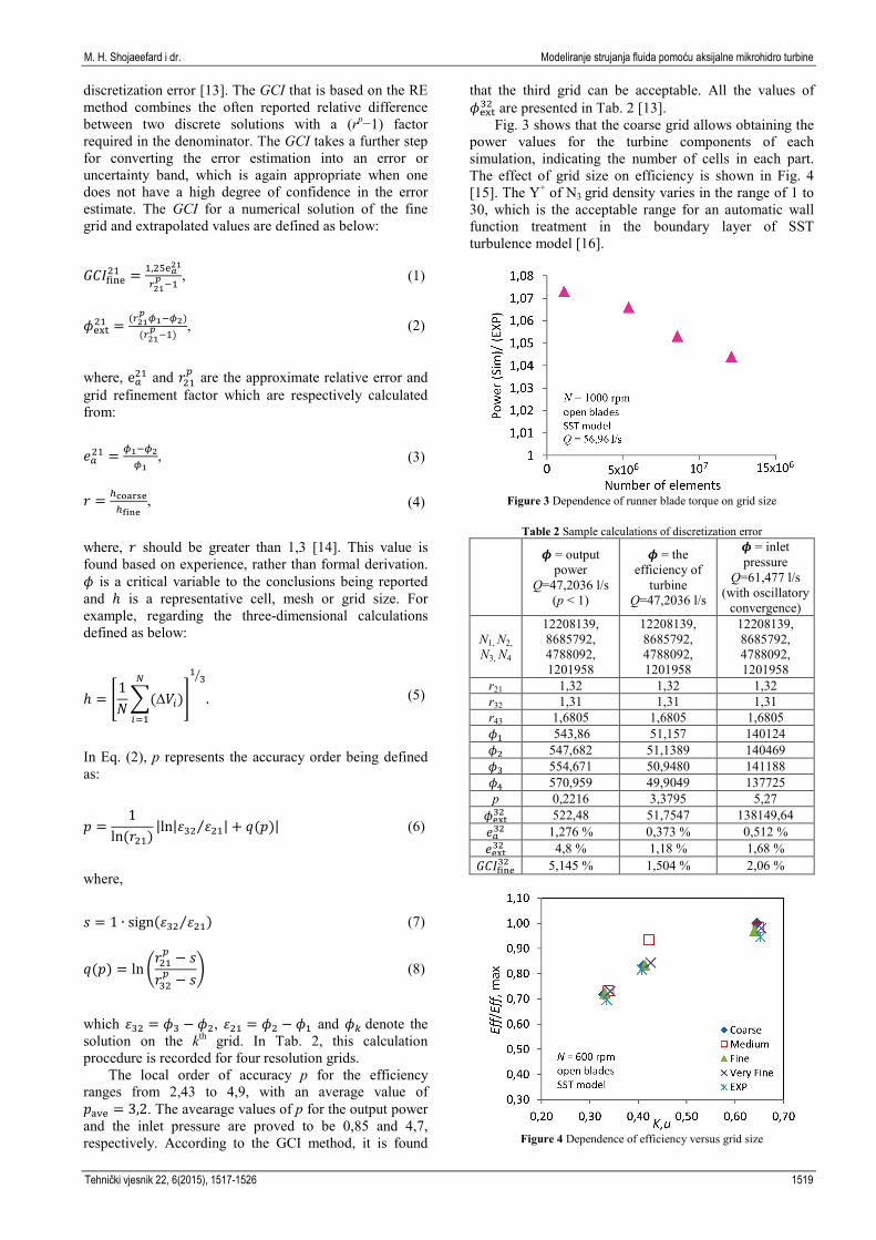
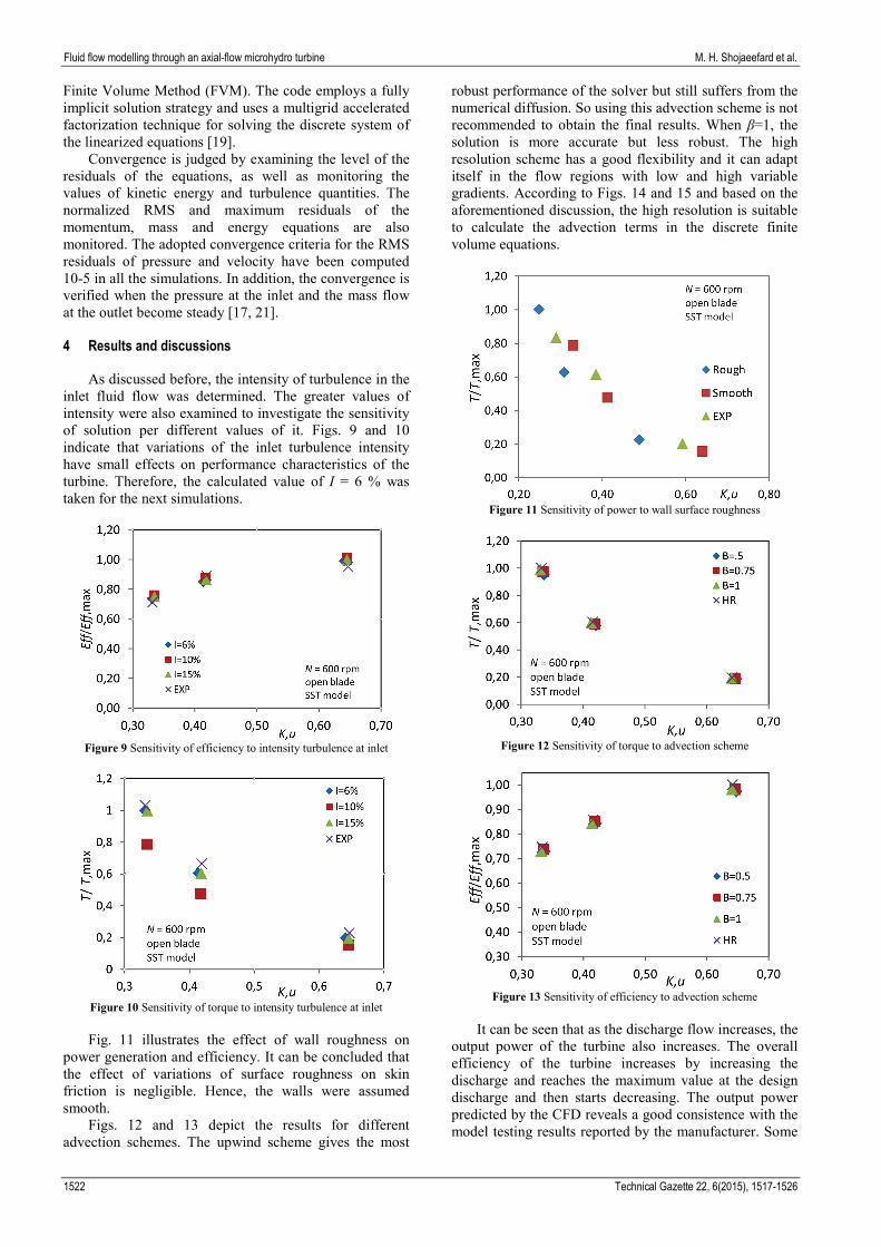
Fig. 3 shows that the coarse grid allows obtaining the power values for the turbine components of each simulation, indicating the number of cells in each part. The effect of grid size on efficiency is shown in Fig. 4 [15]. The Y+ of N3 grid density varies in the range of 1 to 30, which is the acceptable range for an automatic wall function treatment in the boundary layer of SST turbulence model [16].

Figure 3 Dependence of runner blade torque on grid size

Table 2 Sample calculations of discretization error

𝝓𝝓 = inlet pressure

Q=61,477 l/s (with oscillatory

convergence)

𝝓𝝓 = the efficiency of

turbine Q=47,2036 l/s

𝝓𝝓 = output power

Q=47,2036 l/s (p < 1)

12208139, 8685792, 4788092, 1201958

12208139, 8685792, 4788092, 1201958

12208139, 8685792, 4788092, 1201958

N1, N2, N3, N4

1,32 1,32 1,32 r21 1,31 1,31 1,31 r32

1,6805 1,6805 1,6805 r43 140124 51,157 543,86 𝜙𝜙1 140469 51,1389 547,682 𝜙𝜙2 141188 50,9480 554,671 𝜙𝜙3 137725 49,9049 570,959 𝜙𝜙4

5,27 3,3795 0,2216 p 138149,64 51,7547 522,48 𝜙𝜙ext32 0,512 % 0,373 % 1,276 % 𝑒𝑒𝑎𝑎32 1,68 % 1,18 % 4,8 % 𝑒𝑒ext32 2,06 % 1,504 % 5,145 % 𝐺𝐺𝐺𝐺𝐺𝐺fine32

Figure 4 Dependence of efficiency versus grid size



2.2 Grid generation The interaction between the stationary and rotating

domains was modeled by the means of three mathematical interface models: mixing plane, frozen rotor and sliding plane. All these models are common in this fact that they lower the time-dependent interaction between the stator and the rotor domains to a steady-state problem, but they are different in the way how the upstream disturbances are transported across the interface [8].

As shown in Fig. 5, at the mixing plane, the disturbances are averaged circumferentially over the interface, but the frozen rotor ignores this interaction between the rotor and the stator. The most realistic model is the sliding interface in which this transient interaction is correctly predicted.

Figure 5 Three models for rotor-stator interface [8]

To simulate the previously described stage, a mixing

plane model was utilized for the steady-state problems, and the result of the frozen rotor was taken as an initial estimation of the unsteady solution, where the latter, i.e. sliding plane, was implemented for the unsteady simulations.

2.4 Turbulence modelling

The best turbulence model is simply the one that

matches with the experimental data in the best way [17]. Because of producing the virtual diffusion, the standard k-ε model is not suggested for the problems which include intensive non-isotropic and non-equilibrium effects in the flow. In other words, the values of turbulent viscosity were predicted by this model a bit greater. Because of the swirling flow and the curving streamline, the k-ε becomes problematic near the wall regions and cannot model the

boundary layer well. Therefore, this model has a greater difference by the experimental data compared to the other models as illustrated in Figs. 6 and 7. On the other hand, the results of SST are acceptable although not quite accurate. In the SST, separation, swirling flow and reverse gradient near the leading edge and trailing edge are modelling better than k−ω and k−ε. Therefore, the results are nearer to the experimental data in comparison with the k−ε. The EARSM allows an extension of the current k−ε turbulence models to capture the effects of physical phenomena such as secondary flows, flows with streamline curvature and system rotation [13]. Therefore, the obtained results are the same by the two equation models.

Figure 6 Sensitivity of power for different turbulence models

Figure 7 Sensitivity of efficiency for different turbulence models

The SSG model is a new six equation Reynolds stress

model and predicts much more accurately than the k−ε and SST (nevertheless more costly). This model is based on the transport equations for all components of the Reynolds stress tensor and the dissipation rate [4, 18]. Turbulent viscosity term is not in the RSM equations. This makes the solution tend to instability. Existence of the turbulent viscosity in the RANS equations acts as a damper of disturbance and helps to converge the solution. Therefore, with eliminating this term in the RSM model, the numerical instability grows unintentionally and the convergency becomes rather difficult. Most of the turbulent flows demonstrate a non-isotropic nature. In this simulation, the values of principal Reynolds stress are close together. Therefore, the results of the two equation models and RSM are much close. Fig. 8 shows the values of principal stress. According to the results of Figs. 6, 7 and 8, the SST model can lead to the best accuracy, cost and time.



Figure 8 Value of principal stress

2.5 Boundary conditions

The turbine runner was defined in a moving reference

frame with given rotational speed, while the draft tube was considered as a stationary reference frame. Since the simulations are based on the concept of Multiple Frame Reference (MFR), the method of transferring the disturbances between rotating and non-rotating components of the machine should be determined. The interaction between the stationary and rotating domains was modelled by a mixing plane. The outlet of the runner domain and the inlet of the draft tube are taken into account as an interface of the mixing plane.

The measured mass flow rate has been specified at an inlet which is normal to the boundary surface. The averaged static pressure has been set equal to the atmospheric pressure at the outlet boundary, located at the end of the draft tube.

It is also necessary to estimate the turbulence intensity and the length scale at the inlets. Estimating the turbulence intensity in the inlet is often difficult. Because of the high-speed flows inside complex geometries such as those in the turbomachines, the value of intensity normally ranges from 5 % to 20 % [17]. The turbulence intensity, often referred to as the turbulence level, is defined for a fully developed pipe flow as [11]:

𝐺𝐺 = 𝑢𝑢′

𝑈𝑈= 0,16𝑅𝑅𝑒𝑒𝑑𝑑ℎ

−18 , (9)

where 𝑢𝑢′ is the root-mean-square of the turbulent velocity fluctuations and U is the mean velocity. 𝑅𝑅𝑒𝑒𝑑𝑑ℎis the Reynolds number based on the pipe hydraulic diameter, 𝑑𝑑ℎ. The turbulence length scale, L, is a physical quantity describing the size of large energy containing eddies in a turbulent flow. In the pipe flows, this can be estimated from the hydraulic diameter. In a fully developed pipe flow, the turbulence length scale is considered 7 % of the hydraulic diameter. Hence [11]:

𝐿𝐿 = 0,07𝑑𝑑ℎ. (10)

From Eqs. (9) and (10), the intensity and the length

scale were approximated about 6 % and 0,0154 m, respectively. As the bend is located before the turbine, the turbulent intensity was assumed 6 %. In order to

investigate the effect of turbulence intensity, 3 values of that (i.e. 6 %, 10 % and 15 %) were studied.

Being coarse in the physical geometries, the walls are modelled with two smooth and coarse types. The surface roughness may be considered as an aspect of geometry, which leads to an increase in the turbulence near the wall, with a large influence on the boundary layer growth and loss at low and medium Reynolds numbers. If the roughness is known and the boundary layers are fully turbulent, its effect on skin friction can be reasonably predicted. The conventional wall functions are made sensitive to the effects of fine-grain surface roughness through introduction of a dimensionless roughness height. If the average roughness height is denoted by k, then the dimensionless roughness height k+ can be defined in terms of the friction velocity u* [18], by the following equation [11]:

𝑘𝑘+ = 𝑘𝑘𝑢𝑢∗

𝜗𝜗. (11)

3 Solution method

In order to determine the efficiency and power curves and in order to analyse the losses in a draft tube, the steady state simulation is believed to provide acceptable results [15]. Accuracy of the prediction is sensitive to the advection scheme. Upwind, high resolution and some blend factors to blend between the first and second order advection schemes are specified to calculate the advection terms in the discrete finite volume equations. Implementation of the advection schemes can be cast in the following form:

𝜑𝜑point = 𝜑𝜑up + 𝛽𝛽 ∇𝜑𝜑.Δ𝑟𝑟��⃗ , (12)

where 𝜑𝜑up is the value at the upwind node, and 𝑟𝑟 is the vector from the upwind node to the integration point. Particular choices for 𝛽𝛽 and ∇𝜑𝜑 yield different schemes as described below.

By the upwind setting, the advection terms are found of the first-order accuracy. This is equivalent to specifying a blend factor of 0. This scheme is very robust, but it will introduce diffusive discretization errors that tend to steep spatial gradients. A value of 1,0 uses the second order differencing for the advection terms, whereas values between 0,0 and 1,0 blend the first and second order differencing, with an increased accuracy and reduced robustness as β approaches to 1,0. At higher values, some overshoots and undershoots may appear, where excessive diffusivity can occur at lower values. In high resolution setting, the blend factor values vary from 0 to 1. In the flow regions with low variable gradients, the blend factor will be close to 1,0 for more accuracy. In areas where the gradients change sharply, the blend factor will be much closer to 0,0 in order to prevent the possible overshoots and undershoots and also to maintain its robustness [11].

All the numerical solutions for the previously described stage have been attained by OpenFOAM, which is an unstructured multiple element open source code of

http://www.cfd-online.com/Wiki/Hydraulic_diameter



Finite Volume Method (FVM). The code employs a fully implicit solution strategy and uses a multigrid accelerated factorization technique for solving the discrete system of the linearized equations [19].

Convergence is judged by examining the level of the residuals of the equations, as well as monitoring the values of kinetic energy and turbulence quantities. The normalized RMS and maximum residuals of the momentum, mass and energy equations are also monitored. The adopted convergence criteria for the RMS residuals of pressure and velocity have been computed 10-5 in all the simulations. In addition, the convergence is verified when the pressure at the inlet and the mass flow at the outlet become steady [17, 21].

4 Results and discussions

As discussed before, the intensity of turbulence in the

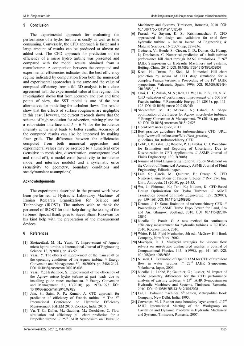
inlet fluid flow was determined. The greater values of intensity were also examined to investigate the sensitivity of solution per different values of it. Figs. 9 and 10 indicate that variations of the inlet turbulence intensity have small effects on performance characteristics of the turbine. Therefore, the calculated value of I = 6 % was taken for the next simulations.

Figure 9 Sensitivity of efficiency to intensity turbulence at inlet

Figure 10 Sensitivity of torque to intensity turbulence at inlet Fig. 11 illustrates the effect of wall roughness on

power generation and efficiency. It can be concluded that the effect of variations of surface roughness on skin friction is negligible. Hence, the walls were assumed smooth.

Figs. 12 and 13 depict the results for different advection schemes. The upwind scheme gives the most

robust performance of the solver but still suffers from the numerical diffusion. So using this advection scheme is not recommended to obtain the final results. When β=1, the solution is more accurate but less robust. The high resolution scheme has a good flexibility and it can adapt itself in the flow regions with low and high variable gradients. According to Figs. 14 and 15 and based on the aforementioned discussion, the high resolution is suitable to calculate the advection terms in the discrete finite volume equations.

Figure 11 Sensitivity of power to wall surface roughness

Figure 12 Sensitivity of torque to advection scheme

Figure 13 Sensitivity of efficiency to advection scheme

It can be seen that as the discharge flow increases, the

output power of the turbine also increases. The overall efficiency of the turbine increases by increasing the discharge and reaches the maximum value at the design discharge and then starts decreasing. The output power predicted by the CFD reveals a good consistence with the model testing results reported by the manufacturer. Some



deviations in the overall efficiency were also noticed; however the trend of both curves was the same.

Poor performance of the draft tube causes drop of the flow and reduces the turbine efficiency. Efficiency of the draft tube which is obtained from the distribution of velocity and pressure at the inlet and outlet is given below [9].

𝐻𝐻𝐿𝐿𝐿𝐿 =𝑃𝑃03 − 𝑃𝑃04

𝛾𝛾 (13)

𝐻𝐻𝑅𝑅𝐿𝐿 =𝑉𝑉32 − 𝑉𝑉42

2𝑔𝑔− 𝐻𝐻𝐿𝐿𝐿𝐿 (14)

𝜂𝜂𝐿𝐿 =2𝑔𝑔 ∗ 𝐻𝐻𝑅𝑅𝐿𝐿

𝑉𝑉32∗ 100 (15)

Figure 14 Efficiency of draft tube

Fig. 14 shows that the maximum efficiency of the

draft tube is 75 %, while the minimum efficiency of the draft tube is 70 % in the worst design of Kaplan turbine [16]. Hence, design of the draft tube has some problem. Maximum cone angle of the draft tube has been mentioned 12° in the literature [22], while cone angle of the available draft tube is 13°. Area ratio of the inlet-outlet and length of the draft tube are also the main parameters for designing the draft tube.

The pressure distribution on the runner is shown in Fig. 15. It can be seen that the flow is accelerated in the runner resulting in a pressure drop. On the suction side of the blades, the velocity maximum can be observed in the same position, where in the minimum pressure could be detected [12].

Figure 15 Pressure distribution on runner

Figure 16 Pressure distribution on runner

Figure 17 Pressure contours in draft tube

Fig. 16 represents the issue of streamlines from

runner cone, contour of axial velocity and vector plot of tangential velocity. The pattern of streamline and pressure contours within the draft tube as shown in Figs. 16 and 17 indicates that a low velocity zone is formed near outlet of the draft tube. The velocity decreases and the pressure increases from the inlet to the outlet of the draft tube due to the increased cross-area of passing flow. This may contribute to increase the power generation in the turbine [17].

Angular velocity of the runner cone plays an important role in creating the separation and thereupon efficiency of the micro turbine. The effect of angular rotation is investigated in the present study. Early separation at end of the hub leads to reduce the effect of the draft tube upon pressure recovery. The separation of recirculation zone increases the average mean velocity, and hence the drops will become greater.

As depicted in figures 18 to 21, the streamlines leave the runner corn for ω=500 to 900 rpm earlier than ω=1200. As angular velocity of the runner cone increases, the swirl decreases. At ω=1200 rpm, the streamlines are straight and attached to the runner cone. The runner cone does not entrain the flow anymore, it decrease intensity of the swirl issued from the runner. The contours of the axial wall shear stress on the runner cone are also illustrated in Figs. 18 to 21. For ω=500, 700 and 900 rpm, the wall shear stress has larger positive values near end of the cone indicating separation. Separation is obtained earlier for ω=500 rpm. This corroborates the fact that the streamlines leave the runner cone earlier for this angular velocity. The separation occurs later for a ω=1200 rpm. This means a better utilization of the cone, i.e. a better pressure recovery. The flow is attached to the runner cone up to end of it [24]. Further experimental study on the draft tube of Agnew microhydro turbine has been presented in [25].



Figure 18 Velocity streamlines and wall shear contours for N=500 rpm of open blades working with 3 pumps






5 Conclusion

The experimental approach for evaluating the performance of a hydro turbine is costly as well as time consuming. Conversely, the CFD approach is faster and a large amount of results can be produced at almost no added cost. The CFD approach for prediction of the efficiency of a micro hydro turbine was presented and compared with the model results obtained from a manufacturer. A comparison between the computed and experimental efficiencies indicates that the best efficiency regime indicated by computation from both the numerical and experimental approaches is the same and the value of computed efficiency from a full-3D analysis is in a close agreement with the experimental value at this regime. The investigation shows that from accuracy and cost and time points of view, the SST model is one of the best alternatives for modelling the turbulent flows. The results show that the effects of surface roughness are negligible in this case. However, the current research shows that the scheme of high resolution for advection, mixing plane for a rotor-stator interface and I = 6 % for the turbulence intensity at the inlet leads to better results. Accuracy of the computed results can also be improved by making finer grids. The difference between the efficiencies computed from both numerical approaches and experimental values may be ascribed to a numerical error (sensitive to mesh size, discretization, convergence level and round-off), a model error (sensitivity to turbulence model and interface models) and a systematic error (sensitivity to geometry, boundary conditions and steady/transient assumptions).

Acknowledgements

The experiments described in the present work have

been performed at Hydraulic Laboratory Machines of Iranian Research Organization for Science and Technology (IROST). The authors wish to thank the personnel of IROST for their help during the testing of the turbines. Special thank goes to Saeed Sharif Razavian for his kind help with the preparation of the measurement devices. 6 References [1] Shojaeefard, M. H.; Yassi, Y. Improvement of Agnew

micro hydro turbine. // International Journal of Engineering Science. 12, 2(2001), pp. 43-52.

[2] Yassi, Y. The effects of improvement of the main shaft on the operating conditions of the Agnew turbine. // Energy Conversion and Management. 50, 10(2009), pp. 2486-2494. DOI: 10.1016/j.enconman.2009.05.036

[3] Yassi, Y.; Hashemloo, S. Improvement of the efficiency of the Agnew micro hydro turbine at part loads due to installing guide vanes mechanism. // Energy Conversion and Management. 51, 10(2010), pp. 1970-1975. DOI: 10.1016/j.enconman.2010.02.029

[4] Jain, S.; Saini, R. P.; Kumar, A. CFD approach for prediction of efficiency of Francis turbine. // The 8th International Conference on Hydraulic Efficiency Measurement, IGHEM 2010, Roorkee, India, 2010.

[5] Vu, T. C.; Koller, M.; Gauthier, M.; Deschênes, C. Flow simulation and efficiency hill chart prediction for a Propeller turbine. // 25th IAHR Symposium on Hydraulic

Machinery and Systems, Timisoara, Romania, 2010. DOI: 10.1088/1755-1315/12/1/012040

[6] Prasad, V.; Sayann, K. S.; Krishnamachar, P. CFD approached for design and validation for axial flow hydraulic turbine. // Indian Journal of Engineering & Material Sciences. 16 (2009), pp. 229-236.

[7] Guénette, V.; Houde, S.; Ciocan, G. D.; Dumas, G.; Huang, J.; Deschênes, C. Numerical prediction of a bulb turbine performance hill chart through RANS simulations. // 26th IAHR Symposium on Hydraulic Machinery and Systems, Beijing, China, 2012. DOI: 10.1088/1755-1315/15/3/032007

[8] Keck, H.; Drtina, P.; Sick, M. Numerical Hill chart prediction by means of CFD stage simulation for a complete Francis turbine. // Proceeding of the 18th IAHR symposium, Valcencia, Spain, 1996. DOI: 10.1007/978-94-010-9385-9_16

[9] Choi, H. J.; Zullah, M. S.; Roh, H. W.; Ha, P. S.; Oh, S. Y. CFD validation of performance improvement of a 500 kW Francis turbine. // Renewable Energy. 54 (2013), pp. 111-123. DOI: 10.1016/j.renene.2012.08.049

[10] Shojaeefard, M. H.; Mirzaei, A.; Babaei, A. Shape optimization of draft tubes for Agnew microhydro turbines. // Energy Conversion & Management. 79 (2014), pp. 681-89. DOI: 10.1016/j.enconman.2013.12.025

[11] OpenFoam users guide, 2011. [12] Best practice guidelines for turbomachinery CFD. URL:

http://www.cfd-online.com/Wiki/Best_practice_ guidelines_for_turbomachinery_CFD

[13] Celik, I. B.; Ghia, U.; Roache, P. J.; Freitas, C. J. Procedure for Estimation and Reporting of Uncertainty Due to Discretization in CFD Applications. // ASME Journal of Fluids Engineering. 130, 7(2008).

[14] Journal of Fluid Engineering Editorial Policy Statement on the Control of Numerical Accuracy, ASME Journal of Fluid Engineering, Editorial paper.

[15] Lain, S.; Garcia, M.; Quintero, B.; Orrego, S. CFD Numerical simulations of Francis turbines. // Rev. Fac. Ing. Univ. Antioquia. 51 (2010), pp. 24-33.

[16] Wu, J.; Shimmei, K.; Tani, K.; Niikura, K. CFD-Based Design Optimization for Hydro Turbines. // ASME Transaction Journal of Fluids Engineering. 129, 2(2007), pp. 159-168. DOI: 10.1115/1.2409363

[17] Denton, J. D. Some limitation of turbomachinery CFD. // Proceedings of ASME Turbo Expo Power for Land, Sea and Air, Glasgow, Scotland, 2010. DOI: 10.1115/gt2010-22540

[18] Nicolle, J.; Proulx, G. A new method for continuous efficiency measurement for hydraulic turbines. // IGHEM-2010, Roorkee, India, 2010.

[19] White, F. M. Fluid Mechanics, 5th ed., McGraw Hill Book Company, New York, 2002.

[20] Mavriplis, D. J. Multigrid strategies for viscous flow solvers on anisotropic unstructured meshes. // Journal of Computational Physics. 145, 1(1998), pp. 141-165. DOI: 10.1006/jcph.1998.6036

[21] Nilsson, H. Evaluation of OpenFOAM for CFD of turbulent flow in water turbines. // 23rd IAHR Symposium, Yokohama, Japan, 2006.

[22] Nicolle, J.; Labbé, P.; Gauthier, G.; Lussier, M. Impact of blade geometry differences for the CFD performance analysis of existing turbines. // 25th IAHR Symposium on Hydraulic Machinery and Systems, Timisoara, Romania, 2010. DOI: 10.1088/1755-1315/12/1/012028

[23] Lal, J. Hydraulic machines, 6th edition, Metropolitan Book Company, New Delhi, India, 1995.

[24] Cervantes, M. J. Runner cone boundary layer control. // 2nd IAHR International Meeting of the Workgroup on Cavitation and Dynamic Problems in Hydraulic Machinery and Systems, Timisoara, Romania, 2007.



[25] Mirzaei, A.; Shojaeefard M. H.; Babaei A.; Yassi Y. Experimental study of redesigned draft tube of an Agnew microhydro turbine. // Energy Conversion and Management. 105, (2015), pp. 488-497. DOI: 10.1016/j.enconman.2015.08.007

Authors’ addresses Mohammad Hasan Shojaeefard, Professor School of Mechanical Engineering, Iran University of Science and Technology Narmak, Tehran, Iran E-mail: [email protected] Ammar Mirzaei, Student of PhD, Corresponding author School of Mechanical Engineering, Iran University of Science and Technology Narmak, Tehran, Iran E-mail: [email protected] Mohamad Sadegh Abedinejad, Student of PhD Institute of Higher Education, (Nongovernmental - Non-profit) Semnan, Iran E-mail: [email protected] Yousef Yassi, PhD Department of Mechanical Engineering, Energy Institute of Higher Education Saveh, Iran E-mail: [email protected]

fluid flow modelling through an axial-flow … fileu ovom je istraživanju analizirano...

Documents