fluid mechanics - a complete theory - tu/e · introduction outline fluid mechanics a complete...
TRANSCRIPT

Introduction Outline
Fluid Mechanicsa complete theory
Peter in ’t panhuis
5th Seminar on Continuum Mechanics
3th May 2006
Introduction Outline
Continuum Mechanics
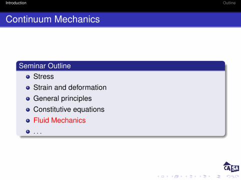
Seminar OutlineStressStrain and deformationGeneral principlesConstitutive equationsFluid Mechanics. . .
Introduction Outline
Fluid Mechanics
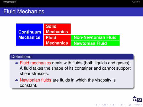
ContinuumContinuumMechanics
SolidMechanicsFluidMechanics
SolidMechanicsNon-Newtonian FluidNewtonian Fluid
Definitions:Fluid mechanics deals with fluids (both liquids and gases).A fluid takes the shape of its container and cannot supportshear stresses.Newtonian fluids are fluids in which the viscosity isconstant.
Introduction Outline
Fluid Mechanics
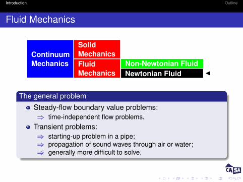
ContinuumContinuumMechanics
SolidMechanicsFluidMechanics
SolidMechanicsNon-Newtonian FluidNewtonian Fluid J
Introduction Outline
Fluid Mechanics
ContinuumContinuumMechanics
SolidMechanicsFluidMechanics
SolidMechanicsNon-Newtonian FluidNewtonian Fluid J
The general problem
Steady-flow boundary value problems:⇒ time-independent flow problems.
Transient problems:⇒ starting-up problem in a pipe;⇒ propagation of sound waves through air or water;⇒ generally more difficult to solve.

Introduction Outline
Outline
1 Field equations of a Newtonian fluidGeneral equationsSimplifications
2 Dimensional analysis3 Special cases
Laminar flow between parallel platesRayleigh problemPerfect fluidAcoustic waves of small amplitudes
4 Potential flowComplex-function formulationFlow past a circular cyclinderConformal mapping methods
5 Summary

Equations Dimensional analysis Special cases Potential flow Summary Further reading
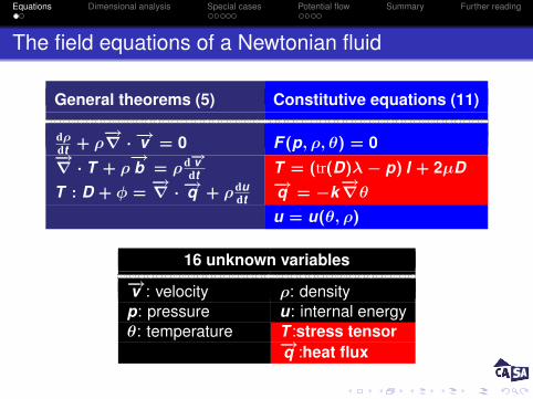
The field equations of a Newtonian fluid
General theorems (5) Constitutive equations (11)
dρdt + ρ
−→∇ · −→v = 0 F (p, ρ, θ) = 0
−→∇ · T + ρ
−→b = ρd−→v
dt T = (tr(D)λ − p) I + 2µDT : D + φ =
−→∇ · −→q + ρdu
dt−→q = −k
−→∇θ
u = u(θ, ρ)
16 unknown variables−→v : velocity ρ: densityp: pressure u: internal energyθ: temperature T : stress tensor
−→q : heat flux
Equations Dimensional analysis Special cases Potential flow Summary Further reading
The field equations of a Newtonian fluid
General theorems (5) Constitutive equations (11)
dρdt + ρ
−→∇ · −→v = 0 F (p, ρ, θ) = 0
−→∇ · T + ρ
−→b = ρd−→v
dt T = (tr(D)λ − p) I + 2µDT : D + φ =
−→∇ · −→q + ρdu
dt−→q = −k
−→∇θ
u = u(θ, ρ)
16 unknown variables−→v : velocity ρ: densityp: pressure u: internal energyθ: temperature T :stress tensor
−→q :heat flux

Equations Dimensional analysis Special cases Potential flow Summary Further reading
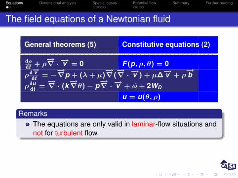
The field equations of a Newtonian fluid
General theorems (5) Constitutive equations (2)
dρdt + ρ
−→∇ · −→v = 0 F (p, ρ, θ) = 0
ρd−→vdt = −
−→∇p + (λ + µ)
−→∇(
−→∇ · −→v ) + µ∆
−→v + ρ−→b
ρdudt =
−→∇ · (k
−→∇θ) − p
−→∇ · −→v + φ + 2WD
u = u(θ, ρ)
7 unknown variables−→v : velocity ρ: densityp: pressure u: internal energyθ: temperature
Equations Dimensional analysis Special cases Potential flow Summary Further reading
The field equations of a Newtonian fluid
General theorems (5) Constitutive equations (2)
dρdt + ρ
−→∇ · −→v = 0 F (p, ρ, θ) = 0
ρd−→vdt = −
−→∇p + (λ + µ)
−→∇(
−→∇ · −→v ) + µ∆
−→v + ρ−→b
ρdudt =
−→∇ · (k
−→∇θ) − p
−→∇ · −→v + φ + 2WD
u = u(θ, ρ)
RemarksThe equations are only valid in laminar-flow situations andnot for turbulent flow.
Equations Dimensional analysis Special cases Potential flow Summary Further reading
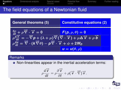
The field equations of a Newtonian fluid
General theorems (5) Constitutive equations (2)
dρdt + ρ
−→∇ · −→v = 0 F (p, ρ, θ) = 0
ρd−→vdt = −
−→∇p + (λ + µ)
−→∇(
−→∇ · −→v ) + µ∆
−→v + ρ−→b
ρdudt =
−→∇ · (k
−→∇θ) − p
−→∇ · −→v + φ + 2WD
u = u(θ, ρ)
RemarksNon-linearities appear in the inertial acceleration terms:
ρd−→vdt
= ρ∂−→v∂t
+ ρ(−→v ·
−→∇)−→v .
Equations Dimensional analysis Special cases Potential flow Summary Further reading
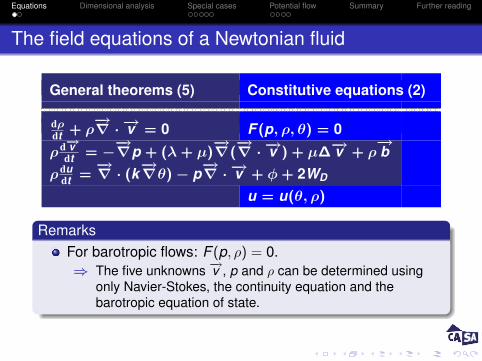
The field equations of a Newtonian fluid
General theorems (5) Constitutive equations (2)
dρdt + ρ
−→∇ · −→v = 0 F (p, ρ, θ) = 0
ρd−→vdt = −
−→∇p + (λ + µ)
−→∇(
−→∇ · −→v ) + µ∆
−→v + ρ−→b
ρdudt =
−→∇ · (k
−→∇θ) − p
−→∇ · −→v + φ + 2WD
u = u(θ, ρ)
RemarksFor barotropic flows: F (p, ρ) = 0.⇒ The five unknowns −→v , p and ρ can be determined using
only Navier-Stokes, the continuity equation and thebarotropic equation of state.
Equations Dimensional analysis Special cases Potential flow Summary Further reading
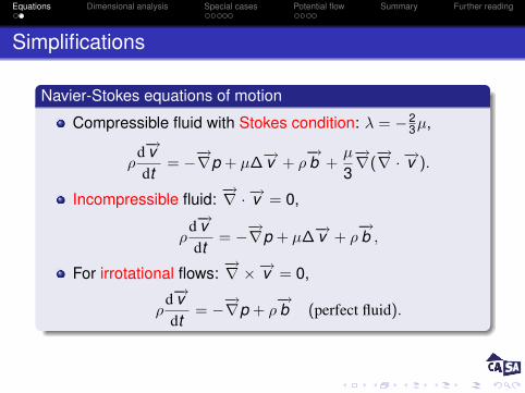
Simplifications
Navier-Stokes equations of motion
Compressible fluid with Stokes condition: λ = −23µ,
ρd−→vdt
= −−→∇p + µ∆
−→v + ρ−→b +
µ
3−→∇(−→∇ · −→v ).
Incompressible fluid:−→∇ · −→v = 0,
ρd−→vdt
= −−→∇p + µ∆
−→v + ρ−→b ,
For irrotational flows:−→∇ ×−→v = 0,
ρd−→vdt
= −−→∇p + ρ
−→b (perfect fluid).
Equations Dimensional analysis Special cases Potential flow Summary Further reading
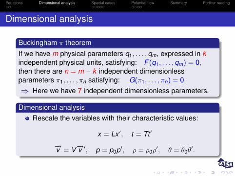
Dimensional analysis
Buckingham π theorem
If we have m physical parameters q1, . . . ,qm, expressed in kindependent physical units, satisfying: F (q1, . . . ,qm) = 0,then there are n = m − k independent dimensionlessparameters π1, . . . , πn satisfying: G(π1, . . . , πn) = 0.⇒ Here we have 7 independent dimensionless parameters.
Dimensional analysisRescale the variables with their characteristic values:
x = Lx ′, t = Tt ′
−→v = V−→v ′, p = p0p′, ρ = ρ0ρ′, θ = θ0θ
′.

Equations Dimensional analysis Special cases Potential flow Summary Further reading
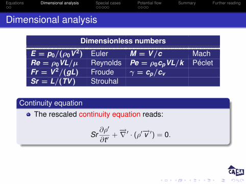
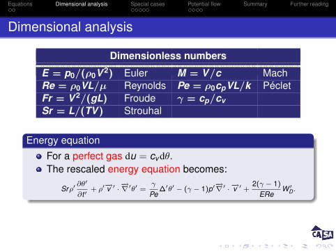
Dimensional analysis
Dimensionless numbers
E = p0/(ρ0V 2) Euler M = V/c MachRe = ρ0VL/µ Reynolds Pe = ρ0cpVL/k PécletFr = V 2/(gL) Froude γ = cp/cvSr = L/(TV ) Strouhal
Navier-Stokes equation
Suppose−→b = −−→g .
The rescaled equations of motion read:
Srρ′ ∂−→v ′
∂t ′+ ρ′−→v ′ · ∇′−→v ′ = −E
−→∇ ′p′ +
1Re
∆′−→v ′ +
13−→∇ ′(
−→∇ ′ · −→v ′)
+
1Fr−→g ′.
Equations Dimensional analysis Special cases Potential flow Summary Further reading
Dimensional analysis
Dimensionless numbers
E = p0/(ρ0V 2) Euler M = V/c MachRe = ρ0VL/µ Reynolds Pe = ρ0cpVL/k PécletFr = V 2/(gL) Froude γ = cp/cvSr = L/(TV ) Strouhal
Continuity equationThe rescaled continuity equation reads:
Sr∂ρ′
∂t ′+−→∇ ′ · (ρ′−→v ′) = 0.
Equations Dimensional analysis Special cases Potential flow Summary Further reading
Dimensional analysis
Dimensionless numbers
E = p0/(ρ0V 2) Euler M = V/c MachRe = ρ0VL/µ Reynolds Pe = ρ0cpVL/k PécletFr = V 2/(gL) Froude γ = cp/cvSr = L/(TV ) Strouhal
Energy equation
For a perfect gas du = cv dθ.The rescaled energy equation becomes:
Srρ′ ∂θ′
∂t ′+ ρ′−→v ′ ·
−→∇ ′θ′ =
γ
Pe∆′θ′ − (γ − 1)p′−→∇ ′ · −→v ′ +
2(γ − 1)
EReW ′
D .
Equations Dimensional analysis Special cases Potential flow Summary Further reading
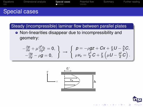
Special cases
Steady (incompressible) laminar flow between parallel platesNon-linearities disappear due to incompressibility andgeometry:
−∂p∂x + µ∂2vx
∂y2 = 0,
−∂p∂y − ρg = 0,
→
p = −ρgz + Cx + µ
h U − h2C,
µvx = y2
2 C + yh
(µU − h2
2 C).

Equations Dimensional analysis Special cases Potential flow Summary Further reading
Special cases
Steady (incompressible) laminar flow between parallel platesNon-linearities disappear due to incompressibility andgeometry:
−∂p∂x + µ∂2vx
∂y2 = 0,
−∂p∂y − ρg = 0,
→
p = −ρgz + Cx + µ
h U − h2C,
µvx = y2
2 C + yh
(µU − h2
2 C).
Couette flow Poiseuille flow
Equations Dimensional analysis Special cases Potential flow Summary Further reading
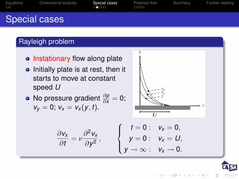
Special cases
Rayleigh problem
Instationary flow along plateInitially plate is at rest, then itstarts to move at constantspeed UNo pressure gradient ∂p
∂x = 0;vy = 0; vx = vx(y , t).
∂vx
∂t= ν
∂2vx
∂y2 ,
t = 0 : vx = 0,y = 0 : vx = U,
y →∞ : vx → 0.
Equations Dimensional analysis Special cases Potential flow Summary Further reading
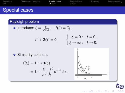
Special cases
Rayleigh problem
Introduce: ξ = y√4νt
, f (ξ) = vxU .
f ′′ + 2ξf ′ = 0,
ξ = 0 : f = 0,
ξ →∞ : f → 0.
Similarity solution:
f (ξ) = 1− erf(ξ)
= 1− 2√π
∫ ξ
0e−x2
dx .
Equations Dimensional analysis Special cases Potential flow Summary Further reading
Special cases
Perfect fluidA perfect fluid is non-viscous and satisfies the Eulerequation
ρd−→vdt
= −−→∇p + ρ
−→b .
At the boundary the normal velocity component is zero.
Kelvin’s theoremIn barotropic flow under conservative body forces, the velocitycirculation Γ around any closed material contour is independentof time.
Γ =
∮∂A
−→v · ds =
∫A(−→∇ ×−→v ) · −→n dS.
⇒ Irrotational flows remain irrotational.

Equations Dimensional analysis Special cases Potential flow Summary Further reading
Special cases
Perfect fluidA perfect fluid is non-viscous and satisfies the Eulerequation
ρd−→vdt
= −−→∇p + ρ
−→b .
At the boundary the normal velocity component is zero.
Bernoulli equation for steady incompressible flowIn steady, incompressible, barotropic flow under conservativebody forces
−→b = −
−→∇Ω,
p +ρ
2V 2 + ρΩ = constant along streamlines (V = |−→v |).
For irrotational flow it is constant everywhere.

Equations Dimensional analysis Special cases Potential flow Summary Further reading
Special cases
Acoustic waves of small amplitudes (1D)Neglecting body forces the 1D Euler and continuityequations are:
∂v∂t
+ v∂v∂x
= −1ρ
∂p∂x,
∂ρ
∂t+∂(ρv)
∂x= 0.
Rescale velocity with speed of sound c:
Srcρ∂v∂t
+ ρv∂v∂x
+ Ec∂p∂x
= 0, Src∂ρ
∂t+∂(ρv)
∂x= 0.
Barotropic equation of state: ρ = ρ(p).
Equations Dimensional analysis Special cases Potential flow Summary Further reading
Special cases
Acoustic waves of small amplitudes (1D)We linearize assuming small Mach number M:
v = Mv1(x , t), p = p0 + Mp1(x , t), ρ = ρ0 + Mρ1(x , t).
Approximate p1 by p1 =(
dpdρ
)0ρ1 =: αρ1 then
Srcρ∂v1
∂t+ Mρv1
∂v1
∂x+αEc
∂ρ1
∂x= 0, Src
∂ρ1
∂t+∂(ρ0v1)
∂x= 0.

Equations Dimensional analysis Special cases Potential flow Summary Further reading
Special cases
Acoustic waves of small amplitudes (1D)We linearize assuming small Mach number M:
v = Mv1(x , t), p = p0 + Mp1(x , t), ρ = ρ0 + Mρ1(x , t).
Approximate p1 by p1 =(
dpdρ
)0ρ1 =: αρ1 then
Srcρ0∂v1
∂t+ αEc
∂ρ1
∂x= 0, Src
∂ρ1
∂t+ ρ0
∂v1
∂x= 0.
v1, p1 and ρ1 all satisfy the wave equation:
∂2Ψ
∂t2 = c20∂2Ψ
∂x2 , c20 =
αEc
Src.
Solution is sum of right and left running wave:
Ψ(x , t) = f (x − c0t) + g(x − c0t).

Equations Dimensional analysis Special cases Potential flow Summary Further reading
Potential flow of incompressible perfect fluids
Potential flowWe consider irrotational, incompressible, perfect fluids.
Irrotational flow:−→∇ ×−→v = 0 −→ −→v =
−→∇φ.
Incompressibility:−→∇ · −→v = ∆φ = 0.
Potential flow in 2D
Continuity equation: ∂vx∂x +
∂vy∂y = 0.
⇒ there exists a function ψ, the stream function, such that
vx =∂ψ
∂yvy = −∂ψ
∂x.
ψ is constant along streamlines.
Equations Dimensional analysis Special cases Potential flow Summary Further reading
Complex-function formulation
Holomorphic functions
A complex function f (z) = u(x , y) + iv(x , y) is holomorphic ifand only if it satisfies the Cauchy-Riemann equations
∂u∂x
=∂v∂y,
∂u∂y
= −∂v∂x
(1)
and u and v have continuous first partial derivatives.⇒ u and v both satisfy Laplace’s equation.⇒ Holomorphic functions are analytic functions.
Equations Dimensional analysis Special cases Potential flow Summary Further reading
Plane potential flow
Complex-function formulation
The complex potential function f (z) = φ(x) + iψ(x) isholomorphic as φ and ψ satisfy Cauchy-Riemann.
Inverse methodExamine various holomorphic complex potential functions andchoose one that’s useful
ExamplesPower series of z within their circle of convergence.Logarithmic potentials away from their points of singularity.⇒ f (z) = az, f (z) = m ln(z − z0).
Equations Dimensional analysis Special cases Potential flow Summary Further reading
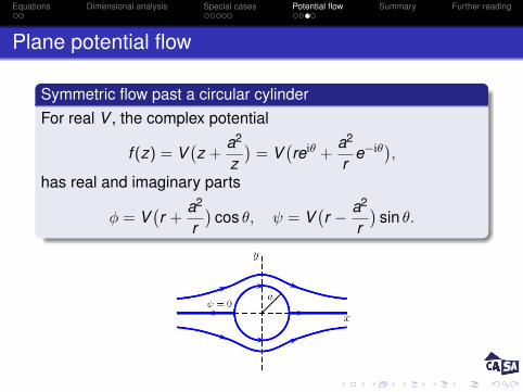
Plane potential flow
Symmetric flow past a circular cylinderFor real V , the complex potential
f (z) = V(z +
a2
z)
= V(reiθ +
a2
re−iθ),
has real and imaginary parts
φ = V(r +
a2
r)
cos θ, ψ = V(r − a2
r)
sin θ.
Equations Dimensional analysis Special cases Potential flow Summary Further reading
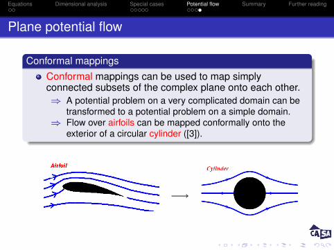
Plane potential flow
Conformal mappings
Conformal mappings can be used to map simplyconnected subsets of the complex plane onto each other.⇒ A potential problem on a very complicated domain can be
transformed to a potential problem on a simple domain.⇒ Flow over airfoils can be mapped conformally onto the
exterior of a circular cylinder ([3]).
−→

Equations Dimensional analysis Special cases Potential flow Summary Further reading
Summary
Fluid mechanics: Newtonian fluidsGeneral theorems:⇒ equations of motion,⇒ continuity equation,⇒ energy equation.
Constitutive equations.Simplifying assumptions:⇒ steady flow,⇒ incompressible flow,⇒ irrotational flow,⇒ Stokes condition,⇒ barotropic fluids,⇒ perfect (inviscid) fluids.

Equations Dimensional analysis Special cases Potential flow Summary Further reading
Further reading
L.E. MalvernIntroduction to the Mechanics of a Continuus MediumPrentice-Hall, 1969.
L.D. Landau and E.M. LifshitzFluid mechanicsPergamon Press, 1959.
L.M. Milne-ThomsonTheoretical HydrodynamicsMacmillan, 1960.
Z. NehariConformal MappingMcGraw-Hill, 1952.