Fluid-Structure interaction applied to blood

flow simulations

J. S. Perez1,E. Soudah1, E. Onate1, J. Garcıa1

A. Mena2, E. Heidenreich2, J. F. Rodrıguez2, M. Doblare2

1International Center for Numerical Methods in Engineering, UPC, Barcelona,Spain

2Group of Structures and Material Modeling. Aragon Institute of EngineeringResearch. University of Zaragoza. Zaragoza, Spain.

Abstract

A coupled fluid-structure interaction model has being developed in order to studythe vessel deformation and blood flow. This paper presents a methodology fromwhich smooth surface are obtained directly form segmented data obtained fromDICOM images. An integrated solution for segmentation-meshing-analysis is alsoimplemented based on the GiD platform.

Key words:PACS:

1 INTRODUCTION

Integration of different disciplines is an important aspects in the current de-velopments of computer applications in biomedical engineering in order to gofrom imagining to computer simulations of tissue, organs, or biological system.Computed Tomography (CT), sometimes called CAT scan, or Magnetic Res-onance Imaging (MRI for short) uses special equipment to obtain image datafrom different angles around the body, and then uses computer processing ofthe information to show a cross-section of body tissues and organs. Using thisinformation, radiologists can more easily diagnose problems such as cancers,cardiovascular disease, infectious disease, trauma and musculoskeletal disor-ders ([1,2]). Due to their detailed information, these tools have become a usefultool in preventive medicine.

These images, on the other hand, can also be used to extract the geometry ofthe organs and tissues for computer analysis via segmentation of the DICOM

Preprint submitted to Elsevier 15 January 2008

image (Digital Imaging and Communications in Medicine). After performingthe segmentation, a discretization of the domain is required for computer sim-ulation. Generating a mesh for Finite Element simulations from a segmentedimage can be cumbersome due to the complicated geometry. To overcome thisproblem, methodologies which make direct use of the segmented data (voxelgeometry) has been proposed [3]. Even though they result useful for elec-trophysiologic simulations, the non-smooth nature of the surface pose seriousproblems in solid mechanics and fluid-structure interaction simulations. There-fore, methodologies which provide smooth surface of the organs and tissuesfrom biomedical images are desirable for computer simulations.

This paper presents a methodology for performing patient-specific computersimulations of cardiovascular systems, in particular fluid-structure interactionin an arterial bifurcation implemented within the Decision Support SystemDSS-DISHEART. The system incorporates a database for managing patientspecific data (i.e., images, cardiovascular data, velocity and pressure profiles,etc), as well as a number of tools for performing image analysis and seg-mentation, meshing and finite element tools, with fluid, structure, and fluid-structure interaction capabilities. It also incorporates a Neural-Network formedical decision support. In the example presented in the paper, the imageof a femoral bifurcation is initially segmented and voxelized to defined the ge-ometry. The voxel data is the used to produce computational meshes for thefluid and solid domains. Biomechanical data from the patient is performed forthe simulations, given more realistic information regarding the performance ofthe particular cardiovascular system. The remaining of the paper is organizedas follows. Section 2 describes the DSS-DISHEART environment. Section 3describes the Methods using for the image processing, segmentation, imagevoxelization and describes the meshing algorithm. Section 4, section 5 andsection 6 detail the fluid and solid solvers and their interaction in FSI simu-lations. Section 7 presents an application in a femoral artery of a patient andsection 8 gives some conclusions.

2 DSS-DISHEART ENVIRONMENT

Previously, more than 5 separate programs were required to create patient-specific geometric models from medical imaging data and perform fluid-structureinteractions in the blood flow simulations. A modular software architecturewas developed Figure 1 to allow the use of best-inclass component technologyand create a single application capable of studying a patient-specific simula-tions. The figure 1 shows the integration environment, a data repository foran abstract data exchange between modules and user, and modules roughlycorresponding to the major tasks in the process. An integrated system wasdeveloped utilizing the architecture shown in Figure 1 that enabled a patient-

2

specific and a technician to go from medical imaging data to analysis results.

Fig. 1. Block diagram depicting processing for a fluid-structure interaction problemof a specific patient. The DICOM file of the patient has been read to the DSS-DIS-HEART Data Base through its interface. To extract the geometry of the analysisVISUAL DICOM is used, after performing the segmentation of the specific domainfor the computer simulation.Subsequently, a new Gid Problem-Type able to visu-alize, manipulate, generate the mesh and impose the specific boundary conditionsfor the fluid and the structure problem over the 3D medical-geometries has beendeveloped. Performed the simulation, the new problem-type will read the resultsand the user can analyze them for this specific case.

As seen in Figure 2, the flowchart of the DSS-DISHEART shows the process toobtain the results of a specific case and how the DSS is created. The Figure 2shows five distinctive parts: definition of the cardiovascular problem, definitionof the data analysis, results, creation and training of the ANN and DecisionSupport System. Each of these parts will be explain in the following points.About the creation and training the ANN and the DSS, further more infor-mation in [4]. The main function of the Database is to store a great amountof medical and material images, to later analyze them and train the neuralnetwork. The Wizard (Figure 3) guides the user through the whole process ofintroducing and analyze an specific case in the database. The different stagesare thus reached in an ordered, synchronized way. The stages that have beensuccessfully finished are depicted in green, and the pending steps are depictedin red. As follows the different steps in a specific patient case are explained.

Step 0: Test name and description. The name of the test to be done is intro-duced, together with a brief description of it.

Step 1: Upload the test image. At this stage the user selects the image inDICOM format to be assigned to the patient. To assign this DICOM, a browseris automatically opened.

3

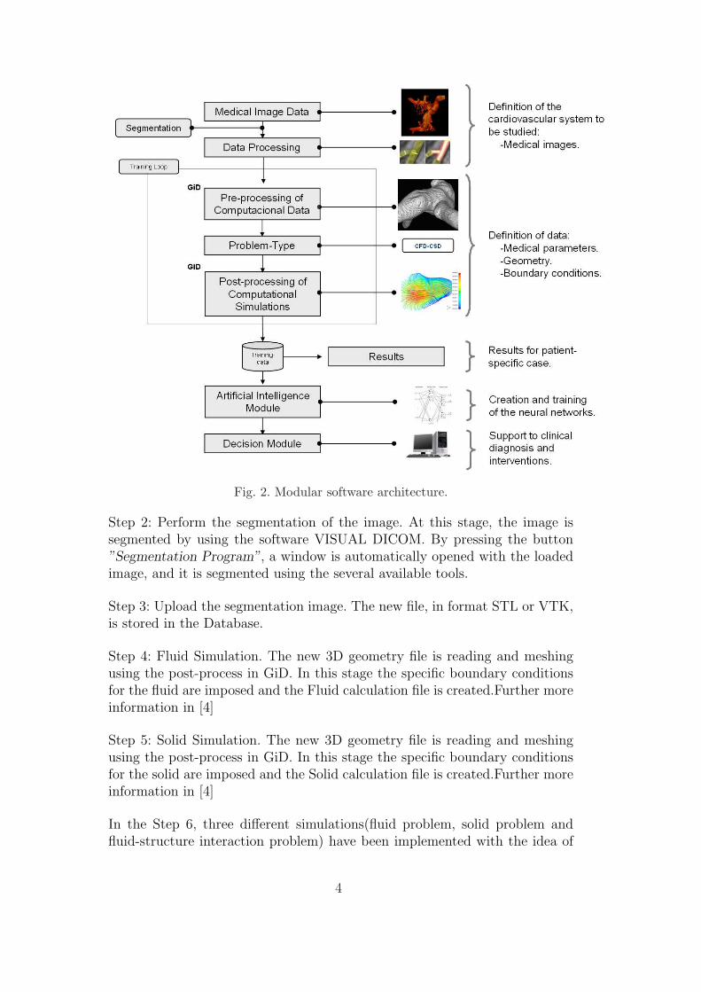
Fig. 2. Modular software architecture.

Step 2: Perform the segmentation of the image. At this stage, the image issegmented by using the software VISUAL DICOM. By pressing the button”Segmentation Program”, a window is automatically opened with the loadedimage, and it is segmented using the several available tools.

Step 3: Upload the segmentation image. The new file, in format STL or VTK,is stored in the Database.

Step 4: Fluid Simulation. The new 3D geometry file is reading and meshingusing the post-process in GiD. In this stage the specific boundary conditionsfor the fluid are imposed and the Fluid calculation file is created.Further moreinformation in [4]

Step 5: Solid Simulation. The new 3D geometry file is reading and meshingusing the post-process in GiD. In this stage the specific boundary conditionsfor the solid are imposed and the Solid calculation file is created.Further moreinformation in [4]

In the Step 6, three different simulations(fluid problem, solid problem andfluid-structure interaction problem) have been implemented with the idea of

4

create a flexibility program. This option gives to the user the possibility ofstudy three different problems, fluid simulation, solid simulation and fluid-structure interaction simulation depending of the specific-case.

In this paper the Interaction simulation was chosen. Then the numerical sim-ulation based on the FEM method starts. When the calculation process hasfinished, the patient case is stored in the Database and can be consulted toverify that the new test has been successfully added.

In order to the system can integrate other input files, the step 2, 4 and 5are optional. This idea gives more flexibility to the system, due to the userhas a VTK file can be upload without the necessity to use VisualDicom, thesegmentation file will save in the database. The same fact happens with thefluid and solid calculation files in the Step 4 and Step 5.

Fig. 3. Segmented image of a human heart.

3 METHODS

3.1 Medical Images.CT image segmentation

The objective of the image segmentation is to find and to identify objectswith certain characteristics form the rest of the image. The data segmenta-tion will allow to visualize and to extract the part of the volume of interest.One of most widely used techniques is the grey thresholding segmentation.It is possibly the simplest and most direct method. The selection of the greythresholds defining the object of interest is usually interactive, even thoughsome alternative techniques have been proposed to determine it in an auto-matic way. These threshold can be defined in either a local or global data set,

5

and sometimes, over a three-dimensional data set.

In most applications, threshold segmentation is accompanied by manual seg-mentation which requires the physician expertise. Figure 4 shows a segmenta-tion of a human heart.

Fig. 4. Segmented image of a human heart.

3.2 Meshing algorithm

The development of finite element simulations in medicine, molecular biologyand engineering has increased the need for quality finite element meshes. Aftersegmenting the medical image we end with a file with the image data and thevalue of the isosurface value defining the boundary of the volumen of interest.The imaging data V is given in the form of sampled function values on recti-linear grids, V = F (xi, yj, zk)|0 ≤ i ≤ nx, 0 ≤ j ≤ ny, 0 ≤ k ≤ nz. We assumea continuous function F is constructed through the trilinear interpolation ofsampled values for each cubic cell in the volume. The format used to read themedical data is VTK structured point as it is agreed in [8]. The description ofthis format can be found in [8]. The image in this format can also be renderedas a volume and manipulated with Itk. Given an isosurface value defining theboundary of the volume of interest we can extract a geometric model of it. Weare interested in creating a distcretization of the volumen suitable for finiteelement computation. In this work we have implemented the following meth-ods to generate the finite element mesh to be used in the analysis stage: i)Dual contouring, ii) Marching cubes, iii) Advancing front, iv) Volume preserv-ing Laplacian smooth. All this methods has being integrated into the generalPre/Post-processor GiD [7].

6

3.2.1 Tetrahedral mesh generation.

In order to generate a tetrahedral mesh from voxels we combine the March-ing Cubes method to generate first the boundary mesh first and then, after asmoothing, an Advancing Front [6] method to fill the interior with tetrahedras.The Marching Cubes [11] algorithm visits each cell in the volume and performslocal triangulation based on the sign configuration of the eight vertices. If oneor more vertex of a cube have values less than the user-specified isovalue, andone or more have values greater than this value, we know the voxel must con-tribute some component of the isosurface. By determining which edges of thecube are intersected by the isosurface, we can create triangular patches whichdivide the cube between regions within the isosurface and regions outside. Byconnecting the patches from all cubes on the isosurface boundary, we get asurface representation.

Some of the triangles generated by the Marching Cubes method does notexhibit good quality to be used in finite element computation. In order toimprove the quality of those elements we apply a laplacian smooth whichvolume preserving. The smoothing algorithm implemented is simple: it try topreserve the volume after each application of the laplace operator by doing anoffset of the vertices along the normals. Figure 5(a) shows the boundary meshgenerated by Marching Cubes and smoothed.

(a) Mesh generated by marching cubes (b) Advancing front

Fig. 5.

The Advancing Front [6] is an unstructured grid generation method. Grids aregenerated by marching from boundaries (front) towards the interior. Tetrahe-dral elements are generated based on the initial front. As tetrahedral elementsare generated, the ”initial front” is updated until the entire domain is coveredwith tetrahedral elements, and the front is emptied. Figure 5(b) shows a cutof the tetrahedral mesh generated by the Advancing Front method.

7

3.2.2 Hexahedral mesh generation

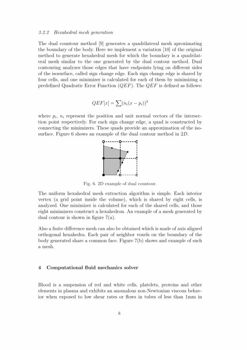
The dual countour method [9] generates a quadrilateral mesh aproximatingthe boundary of the body. Here we implement a variation [10] of the originalmethod to generate hexahedral mesh for which the boundary is a quadrilat-eral mesh similar to the one generated by the dual contour method. Dualcontouring analyzes those edges that have endpoints lying on different sidesof the isosurface, called sign change edge. Each sign change edge is shared byfour cells, and one minimizer is calculated for each of them by minimizing apredefined Quadratic Error Function (QEF ). The QEF is defined as follows:

QEF [x] =∑

(ni(x− pi))2

where pi, ni represent the position and unit normal vectors of the intersec-tion point respectively. For each sign change edge, a quad is constructed byconnecting the minimizers. These quads provide an approximation of the iso-surface. Figure 6 shows an example of the dual contour method in 2D.

Fig. 6. 2D example of dual countour.

The uniform hexahedral mesh extraction algorithm is simple. Each interiorvertex (a grid point inside the volume), which is shared by eight cells, isanalyzed. One minimizer is calculated for each of the shared cells, and thoseeight minimizers construct a hexahedron. An example of a mesh generated bydual contour is shown in figure 7(a).

Also a finite difference mesh can also be obtained which is made of axis alignedorthogonal hexahedra. Each pair of neighbor voxels on the boundary of thebody generated share a common face. Figure 7(b) shows and example of sucha mesh.

4 Computational fluid mechanics solver

Blood is a suspension of red and white cells, platelets, proteins and otherelements in plasma and exhibits an anomalous non-Newtonian viscous behav-ior when exposed to low shear rates or flows in tubes of less than 1mm in

8

(a) Hexahedral mesh generatedby dual contour method

(b) Finite difference mesh

Fig. 7.

diameter. However, in large arteries, vases of medium calibre as well as cap-illaries, the blood may be considered a homogeneous fluid, with ”standard”behaviour(Newtonian fluid)[29].

The governing equations for blood flow used in this work are the Navier-Stokesequations, with the assumptions of incompressible and Newtonian flow(90%of the blood is water). For the representation of the Navier-Stockes equationson the deforming fluid domain Ω of the AAA model based on the arbitraryLagrangianEulerian (ALE) method[28], we adopt the following notation: Ω is athree-dimensional region denoting the portion of the district on which we focusour attention, and x=(x1, x2, x3) is an arbitrary point of Ω ; v=v(x, t) denotesthe blood velocity. For x ε Ω and t>0 the conservation of momentum andcontinuity in the compact form are described by the following equations(1):

ρ ·(

∂u

∂t+ (u · 5u)

)+∇ p−∇ · (µ4 u) = ρ · f in Ω(0, t)

∇u = 0 in Ω(0, t)

(1)

where u = u (x, t) denotes the velocity vector, p = p (x, t) the pressure field,ρdensity, µ the dynamic viscosity of the fluid and f the volumetric accelera-tion. Blood flow is simulated for average blood properties: molecular viscosityµ =0.0035 Pa.s and density ρ =1050 kg/m3. The volumetric forces(ρ · f) arenot taken in to account in the present analysis.

The boundary conditions for the pulsatile flow, the inflow mean velocityis time-dependent and the volumetric flow rate is oscillatory, as shown in

9

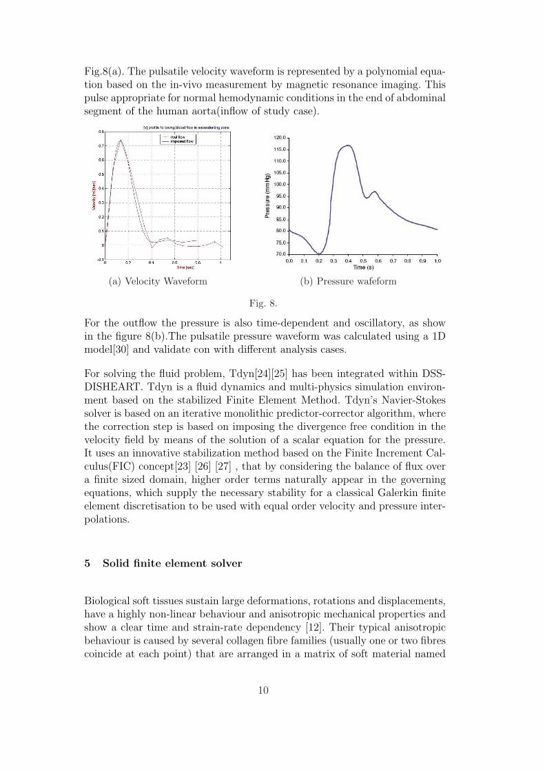
Fig.8(a). The pulsatile velocity waveform is represented by a polynomial equa-tion based on the in-vivo measurement by magnetic resonance imaging. Thispulse appropriate for normal hemodynamic conditions in the end of abdominalsegment of the human aorta(inflow of study case).

(a) Velocity Waveform (b) Pressure wafeform

Fig. 8.

For the outflow the pressure is also time-dependent and oscillatory, as showin the figure 8(b).The pulsatile pressure waveform was calculated using a 1Dmodel[30] and validate con with different analysis cases.

For solving the fluid problem, Tdyn[24][25] has been integrated within DSS-DISHEART. Tdyn is a fluid dynamics and multi-physics simulation environ-ment based on the stabilized Finite Element Method. Tdyn’s Navier-Stokessolver is based on an iterative monolithic predictor-corrector algorithm, wherethe correction step is based on imposing the divergence free condition in thevelocity field by means of the solution of a scalar equation for the pressure.It uses an innovative stabilization method based on the Finite Increment Cal-culus(FIC) concept[23] [26] [27] , that by considering the balance of flux overa finite sized domain, higher order terms naturally appear in the governingequations, which supply the necessary stability for a classical Galerkin finiteelement discretisation to be used with equal order velocity and pressure inter-polations.

5 Solid finite element solver

Biological soft tissues sustain large deformations, rotations and displacements,have a highly non-linear behaviour and anisotropic mechanical properties andshow a clear time and strain-rate dependency [12]. Their typical anisotropicbehaviour is caused by several collagen fibre families (usually one or two fibrescoincide at each point) that are arranged in a matrix of soft material named

10

ground substance [12]. Typical examples of fibred soft biological tissues areblood vessels, tendons, ligaments, cornea and cartilage. Therefore, in to beable to capture the nonlinear anisotropic hyperelastic behavior, it is neces-sary to consider the formulation of finite strain hyperelasticity in terms ofinvariants with uncoupled volumetric-deviatoric responses, first suggested in[13,14], generalized in [15], and employed for anisotropic soft biological tissuesin [16,17].

Let F = ∂x/∂X be the deformation gradient mapping a point X in the ref-erence configuration to a point x in the current configuration. Further, letJ = det(F) be the jacobian of the motion. Proper volumetric and deviatoricuncoupled responses can be defined following the kinematic decomposition

F = J1/3F, C = FT F, (2)

where F is deviatoric deformation gradient, and C is the right Cauchy-Greentensor associated to F. Let a0 and b0 be the directions of collagen fiberswithin the tissue defining the transverse anisotropic behavior of the tissue[17]. For isothermal processes, we can postulate the existence of a uniquedecoupled representation of a strain-energy density function Φ[18]. Based onthe kinematic decomposition (2), and following[13,17] the free energy for ananisotropic hyperelastic soft tissue can be written in a decoupled form as

Φ(C, a0,b0) = U(J) + Φ(I1, I2, I4, I6), (3)

with

I1 = trC, I2 = 1/2(tr(C)2 − trC2),

I4 = a0 · C · a0, I6 = b0 · C · b0,(4)

I1 and I2 are the invariants of C, and I4 and I6 are the square of the stretchesalong a0 and a0 respectively. For a hyperelastic material, the 2nd Piola-Kirchoff stress is derived from the strain energy as S = 2∂Φ/∂C. For theform of the strain energy given in Eq. (3), the 2nd Piola-Kirchoff and Cauchystress, σ, tensors, with the later obtained as the weighted push forward of S,can be written as

S = U ′JC−1 + 2J−2/3DEV[

∂Φ∂C

], σ = U ′1 + 2

Jdev

[F ∂Φ

∂CFT

], (5)

where DEV[·] = [·]− 13([·] : C)C−1, and dev[·] = [·]− 1

3([·] : 1)1.

In terms of the free energy, the total energy of the system is then given by thefunctional

Π(u) =∫

ΩΦ(X,Ca0,b0)dV + Πext(u), (6)

where the explicit dependence on X accounts for the heterogeneity, and Πext

is the potential energy of the external loading. The finite element formulation

11

is based in the minimization of Eq. (6), which first variation with respect tou along the direction η is given by

DuΠ(u) · η =∫

Ω[σ : ∇η − gext(η)]dV, (7)

where σ is de Cauchy stress and gext is the virtual work of the external loading.Even though Eq. (7) is valid for compressible solids and refer to this to keepthe exposition simple, for a quasi-incompressible formulation the reader isreferred to [15,16].

Introducing the standard finite element approximation, u =∑Nnod

k=1 = Nkuk,with uk ∈ R3, and N the isoparametric interpolation functions, into Eq. (7)leads to a nonlinear system of equations. Restricting Eq. (7) to a single element

Ge(u,η)|ωe =∫

2[σe : ∇sη]Jejξdξ]dV − gext(η)|ωe = 0, (8)

where jξ is the jacobian of the isoparametric mapping, and the integral iscarried on the unit cube [16]. The solution of this system of equations for agiven increment ∆u is performed iteratively by means of Newtons method,by consistent linearization of Eq. (8) about the displacement in the currentiteration. The linearized for of Eq. (8) at iteration k is given by

LukGe(u) = Ge(uk) + DGe(u

k) ·∆(u). (9)

This linearization leads to a linear system of equations at the element level ofthe form

Ke = ∆ue = Fext − Fint, (10)

where Ke stands for the element stiffness matrix. After imposing proper bound-ary conditions to the global system of equations, solving for ∆u, allows tocompute an approximation to the displacement field at iteration k + 1 asuk+1 = uk+1 + ∆u.

6 Numerical study of the coupled fluid-structure problem

A distinctive feature of the fluid-structure problem is the coupling of twodifferent sub-problems, the first referring to the fluid (whose solution is char-acterized by the pressure and turbulence fields of the blood) and the secondto the structure (whose unknown variable is the displacement field of the vas-cular wall). To match the two solvers, we can proceed in many different ways.Similarly, different strategies can be considered for the computation of the gridvelocity in the ALE perspective. In this section, we illustrate, in particular,an explicit algorithm for the coupling of fluid and structure.

12

To consider the problem arising when coupling fluid and structure models,let us restrict our analysis to a domain Ω . The boundary Γ is composed ofa portion ΓC , which is assumed to be compliant, and a part ΓF , which isassumed to be fixed.

Let us consider the interface conditions between the fluid and the structure.The first condition ensures the continuity of the velocity field, and reads:

v = η x ∈ ΓC (11)

where η is the velocity field of the vessel.

The fluid exerts a surface force field over the vessel (we will neglect the possiblestresses excreted by the surrounding organs in our analysis). These forces mustbe treated as a (Neumann) boundary data for the structure problem:

Φ = −Pn + nS x ∈ ΓC (12)

where Φ is the forces field vector applied in the vessel due to the blood flow.

The fluid-structure interaction problem we deal with is therefore specified by(1),(11),(12) and the governing equations of the vessel model. In view of itsnumerical solution, the coupled problem ought to be split at each time stepinto two sub-problems, one in Ω , the other on Ωs (the vessel domain), com-municating to one another through the matching conditions (11) and (12).In particular, the structure problem provides the boundary data for the fluidproblem; vice-versa, the fluid problem provides the forcing term for the struc-ture.

6.1 Numerical Solution

The coupled problem is split at each time into a structure and a fluid prob-lem, communicating with one another through boundary terms: a forces fieldboundary term in the vessel due to the fluid and a velocity restriction of theboundary ΓC of the fluid. Figure (9) shows the basic steps of the algorithmwhich we are going to illustrate for advancing from time level n to time leveln+1

V and P respectively as usual will denote the unknowns referring to thevelocity and pressure, while the ones relative to the structure are denoted byH.

13

Vessel Wall Structure Solver

?

-

New Domain Configuration

Boundary VelocityGrid velocity(w)

Blood Fluid Solver(Tdyn)

Boundary Conditions on

ν = µ on ΓC

on ΓC

Fig. 9. Representation of the splitting in two sub-problem for our approach (coupledsolver).

The algorithm iteration process for each time step can be resumed as follows:

a) Solving the structure problem (vessel wall) with the boundary terms due tothe blood flow. At the first time level, the scheme is suitable modified, takinginto account the initial data on the position and the velocity at time t=0.

b) Updating domain configuration and boundary conditions for the fluid solver:Once Hn+1 is known, we can compute the domain deformations and the move-ment of the nodes of the grid for the fluid. The new position of the boundaryΓC is computed through the relation:

xn+1i = x0

i + ηn+1i (13)

The displacement of the nodes of the grid for the fluid is obtained as a diffusedinto the fluid domain of the boundary displacement. Diffusion process is basedon an arrangement by levels of the mesh nodes, where level 0 corresponds tothe mesh nodes on the ship surface, level 1 to the nodes connected to level 0nodes, and so on.

The velocity mesh, w, is computed by the equation:

wn+1 =1

∆t· (xn+1 − xn) (14)

The idea underlying this approach is to take advantage of the regularizationdue to the inversion of the Laplace operator in order to have an acceptablemesh. From time to time, however, it could be necessary to remesh the wholedomain, if the grid is too distorted after a certain number of steps.

Another strategy consists of computing the velocity mesh as the solution ofthe problem:

14

−∆wn+1 = 0 in Ω(0, t)

wn+1 = ηn+1 on ΓC(0, t)

wn+1 = 0 on ΓF (0, t)

(15)

Finally, the mesh update is obtained by:

xn+1 = xn + ∆t · wn+1 (16)

For a comparison of the two strategies, see [21].

Fig. 10. Updating of the Mesh.

Solving the blood flow problem

c) The ALE formulation of the Navier-Stockes equations (1) is solved by im-plicit 2nd order accurate projection schemes. The choice of the time-advancingmethod satisfies the Geometric Conservation Laws.

d) Computing the force field applied as a boundary condition in the structureproblem due to the fluid.

When the boundary nodes of the structure and the fluid are not coincident isnecessary to make an interpolation of the nodal quantities during the inter-action algorithm. The methodology used for this interpolation is based on anocttree search algorithm of elements and standard finite element techniques.

This algorithm performs a staggered coupling between the fluid and the struc-ture problems; therefore, it should generally undergo stability limitations onthe time step. These limitations could turn out to be restrictive in practicalcomputations.

15

7 RESULTS

7.1 Femoral Artery

An example of a human femoral bifurcation is considered in this section todemonstrate de methodology. The patient was injected with XXX mL of con-trast agent into a peripheral vein .Images of the femoral bifurcation werecaptured in a 16 Detector/16 Slice Toshiba Multidetector CT Scanner using aslice thickness of 3.2 mm with slices reconstructed every 1.6 mm to maximizelongitudinal resolution. Images were reconstructed using Maximum-Intensity-Projection (MIP) algorithm in the frontal and sagittal views.

Arterial segmentation has been automatically performed by means of thresh-old segmentation using the Visual DICOM software within DSS-DISHEART.Figure 11(a) shows the voxel representation of the geometry of the bifurcation.From the voxel representation, the mesh has been generated by the MarchingCubes method and then smoothed as illustrated in figure 11(b).

(a) Voxel representation of thefemoral bifurcation (VTK format)

(b) Mesh generated of the femoralbifurcation(GiD format)

Fig. 11.

From the voxel image given in figure 11(a), surface and solid meshes have beencreated for the fluid and solid domains using the software GiD within the DSS-DISHEART. The resulting meshes were 3003 hexahedral finite elements forthe solid wall and 74125 tetrahedral elements for the fluid. Figure 12 showthe meshes for the solid (arterial wall) and the fluid respectively. The solidmesh for the arterial wall has been generated by extruding the surface mesha uniforme thickness of 1.5mm.

16

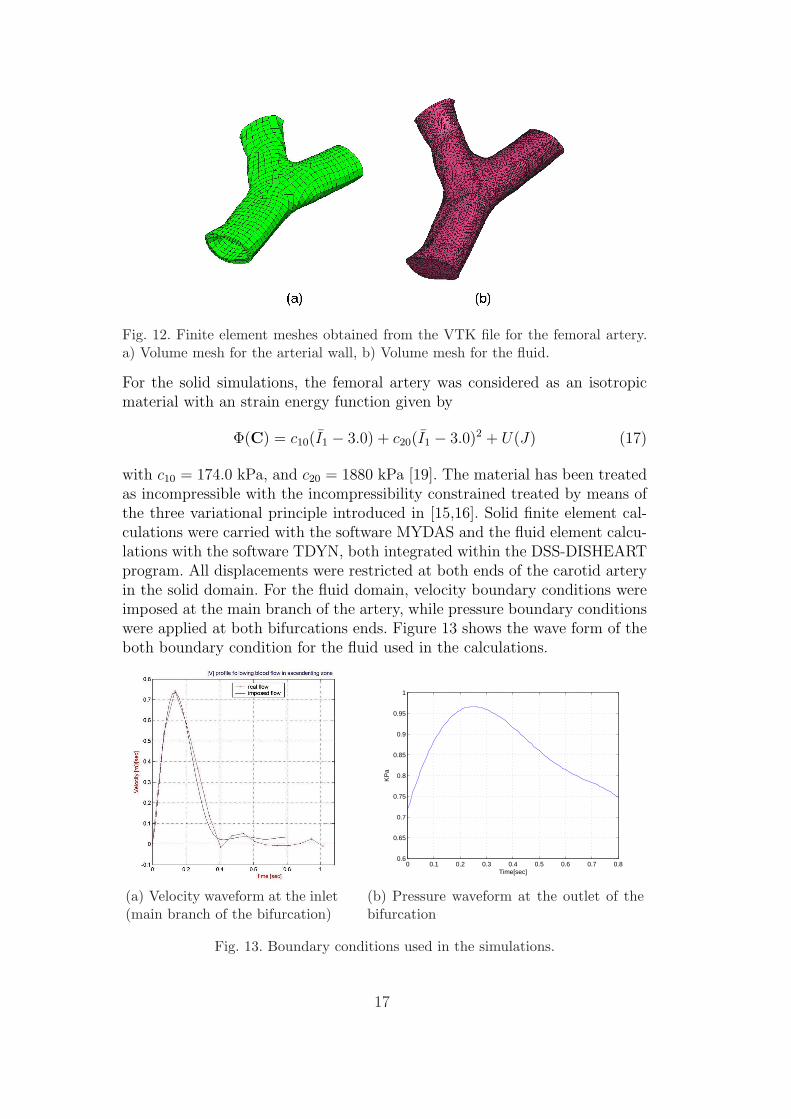
Fig. 12. Finite element meshes obtained from the VTK file for the femoral artery.a) Volume mesh for the arterial wall, b) Volume mesh for the fluid.

For the solid simulations, the femoral artery was considered as an isotropicmaterial with an strain energy function given by

Φ(C) = c10(I1 − 3.0) + c20(I1 − 3.0)2 + U(J) (17)

with c10 = 174.0 kPa, and c20 = 1880 kPa [19]. The material has been treatedas incompressible with the incompressibility constrained treated by means ofthe three variational principle introduced in [15,16]. Solid finite element cal-culations were carried with the software MYDAS and the fluid element calcu-lations with the software TDYN, both integrated within the DSS-DISHEARTprogram. All displacements were restricted at both ends of the carotid arteryin the solid domain. For the fluid domain, velocity boundary conditions wereimposed at the main branch of the artery, while pressure boundary conditionswere applied at both bifurcations ends. Figure 13 shows the wave form of theboth boundary condition for the fluid used in the calculations.

(a) Velocity waveform at the inlet(main branch of the bifurcation)

0 0.1 0.2 0.3 0.4 0.5 0.6 0.7 0.80.6

0.65

0.7

0.75

0.8

0.85

0.9

0.95

1

Time[sec]

KP

a

(b) Pressure waveform at the outlet of thebifurcation

Fig. 13. Boundary conditions used in the simulations.

17

Figure 14 shows the displacement filed of the solid wall and of the ALE-meshat the instant of maximum pressure. The figure demonstrate the effectivecoupling achieved between the solid and the fluid solvers.

(a) Magnitude of the displacement ofthe solid wall in (mm)

(b) Displacement of the ALE-meshin (mm)

Fig. 14. Displacement field for the couple problem. The figure demonstrate theeffective coupling achieved between the solid and fluid solvers.

Figure 15 shows the stress field in the arterial wall and the velocity field inthe artery mid-plane. As expected with incompressible fluids, the maximumstress in the arterial wall occurs at the section were fluid velocity reduces sinceit implies an increment in the local pressure.

(a) Stress field in (kPa) (b) Velocity field in (mm/sec)

Fig. 15. Stress and velocity fields in the artery at the time of maximum pressure.

8 CONCLUSIONS

The results show the viability of applying the presented methodology to gen-erate computational finite element meshes from segmentation files obtainedfrom medical images. This tool opens new possibilities for patient specificbiomechanical applications.

18

9 ACKNOWLEDGMENTS

The authors would like to thank Dr.Franesc Carreras and the Cardiology Unitat Sant Pau University Hospital Barcelona for his work on generation of themedical images and their technical support. Financial support for this researchwas provided by the European Research Area under the Sixth FrameworkProgram CRAFT-Project.

References

[1] Fasel, J.H.D., Selle D., Evertsz, C.J.G., Terrier, F., Peitgen, H.O., Gailloud,P. Segmental anatomy of the liver: poor correlation with CT, Radiology.206(1998):151-156.

[2] Goldin JG, Ratib O, Aberle DR. Contemporary cardiac imaging: an overview. JThorac Imaging. 15(4)(2000):218-29.

[3] Heidenreich, E., Mena A, Rodrıguez J.F., Olmos, S., Doblare M. Simulacionde electrofisologıa cardiaca de imagenes medicas. Modelos numericos especıficosa pacientes. Congreso Annual de la Sociedad Espanola de IngenierıaBiomedica.,Pamplona, 6-8 November 2006. Pamplona, Spain.

[4] E.Soudah,J.F.Rodrıguez,M.Bordone,E.Heidenreich,M.Doblare,E.Onate.”Gridbased decision support system for assisting clinical diagnosis and interventionsin cardiovascular problems.” M-IS88,ISBN:88-95999-87-1, Vol 1, Vol 2. CIMNE,2007.

[5] Marmion M, Deutsch E. Tracers and contrast agents in cardiovascular imaging:present and future. Q. J. Nucl. Med. 40(1)(1996):121-31.

[6] R. Lohner, P. Parikh. Three dimensional grid generation by the advancing-frontmethod. International Journal for Numerical Methods in Fluids, 8(1988):1135-1149, 1988.

[7] GiD - The personal pre and postprocessor, http://www.gidhome.com/,CIMNE,2006.

[8] VTK File Formats,Kitware Inc, http://www.vtk.org/pdf/file-formats.pdf, 2006.

[9] T. Ju, F. Losasso, S. Schaefer, and J. Warren. Dual contouring of hermite data.In Proceedings of SIGGRAPH (2002), pp. 339-346.

[10] Yongjie Zhang and Chandrajit Bajaj and Bong-Soo Sohn, ”SM’03: Proceedingsof the eighth ACM symposium on Solid modeling and applications”, 2003, 286-291, New York, NY, USA, ACM Press.

[11] W. E. Lorensen and H. E. Cline. Marching cubes: A high reso-lution 3d surfaceconstruction algorithm. In Proceedings of SIGGRAPH, pages 163-169, 1987.

19

[12] Humphrey, J.D. Cardiovascular solid mechanics, Springer, New York, 2002.

[13] Spencer, A. J. M. Theory of Invariants, In Continuum Physics, 239-253,Academic Press, New York, 1954

[14] Flory, P. J. Thermodynamic relations for high elastic materials. Transactionsof the Faraday Society, 57:829-838, 1961

[15] Simo, J. C., Taylor, R. L. Quasi-Incompresible Finite Elasticity in PrincipalStretches. Continuum Basis and Numerical Algorithms, Comput Methods ApplMech Engrg, 85:273-310, 1991

[16] Weiss, J.A., Maker, B.N., Govindjee, S. Finite element implementation ofincompressible, transversely isotropic hyperelasticity, Comput Methods ApplMech Engrg, 135:107-128, 1996

[17] Holzapfel, G.A., Gasser, C.T. and Ogden, R.W. A new constitutive frameworkfor arterial wall mechanics and a comparative study of material models. J.Elasticity, 61:1-48, 2000

[18] Ciarlet, PG. Mathematical Elasticity. Vol I: Three dimensional elasticity.Elsevier science publishers, 1991.

[19] Ballyk, P.D., Walsh C., Butany J., Ojha, M. Compliance mismatch mypromote graft-artery intimal hyperplasia by altering suture-line stresses. Journalof Biomechanics, 31: 229-237.

[20] Cokelet, G.: The Rheology and Tube Flow of Blood. In:Shalak, R., Chen, S.(eds.) Handbook of bioengineering. New York: McGraw-Hill 1987.

[21] Nobile, F.: Numerical approximation of Fluid-Structure interaction problemswith application to hemodynamics. PhD thesis-2001. Ecole PolytechniqueFederale de Lausanne(EPFL) Thesis N 2458

[22] J. Garcıa, E. Onate,Journal of Applied Mechanics.”An Unstructured FiniteElement Solver for Ship Hydrodynamics Problems”, ASME, New York(USA),January-03,ISSN 0021-8936.

[23] E. Onate, A.Valls, J. Garcıa, ”Computational Mechanics”,”FIC/FEMformulation with matrix stabilizing terms for incompressible flows at low and highReynolds numbers”, Springer Berlin / Heidelberg, 2006 ISSN: 0178-7675 (Paper)1432-0924 (Online)

[24] COMPASS Ingeniera y Sistemas SA.Tdyn. Environment for Fluid Dynamics(Navier Stokes equations), Turbulence, Heat Transfer, Advection of Species andFree surface simulation. Theoretical background and Tdyn 3D tutorial. March2002.

[25] E. Onate,J. Garcıa, S.R. Idelsohn and F. del Pin,”Computer Methods inApplied Mechanics and Engineering”, ”Finite calculus formulation for finiteelement analysis of incompressible flows. Eulerian, ALE and Lagrangianapproaches” Elsevier,Laussane (Switzerland),2006,ISSN 0045-7825.

20

[26] E. Onate, A.Valls, J. Garcıa,”Journal of Computational Physics”,”ModelingIncompressible Flow at Low and High Reynolds Numbers via a Finite Calculus-Finite Element Approach”,Elsevier,New York (USA) 2007,ISSN 0021-9991.

[27] E. Onate, A.Valls, J. Garcıa,”International Journal for Numerical Methodsin Fluids”,”Computation of turbulent flows using a finite calculus-finite elementformulation”,John Wiley And Sons, London (GB)2007,ISSN 0271-2091.

[28] Formaggia,L.,Nobile,F.Quarteroni,A.,Veneziani,A.(1999).Multiscale modellingof the circulatory system: a preliminary analysis.Comput.Visual.Sci.2, 75-83

[29] Perktold, et al., Pulsatile non-Newtonian Blood Flow in Three-DimensionalCarotid Bifurcation Models: A Numerical Study of Flow Phenomena UnderDifferent Bifurcation Angles, Nov. 1991, J. Biomed. Eng., vol. 13, pp. 507-515

[30] E.Soudah, F.Mussi and E.Onate. ”Validation Of The One-DimensionalNumerical Model In The Ascending-Descending Aorta With Real Flow Profile”.IIIInternational Congress on Computational Bioengineering (ICCB 2007) Venezuela.

21