FLUID SUBSTITUTION AND AVAZ ANALYSIS OF

FRACTURED DOMAINS: AN ULTRASONIC

EXPERIMENTAL STUDY

A Thesis

Presented to

the Faculty of the Department of Earth and Atmospheric Sciences

University of Houston

In Partial Fulfillment

of the Requirements for the Degree

Master of Science

By

Long Huang

August, 2013

FLUID SUBSTITUTION AND AVAZ ANALYSIS OF

FRACTURED DOMAINS: AN ULTRASONIC

EXPERIMENTAL STUDY

Long Huang

APPROVED:

Dr. Robert Stewart, Committee ChairDepartment of Earth and Atmospheric Sciences

Dr. Evgeny Chesnokov, Committee memberDepartment of Earth and Atmospheric Sciences

Dr. Samik Sil, Committee memberConocoPhillips

DeanCollege of Natural Sciences and Mathematics

ii

Acknowledgements

First, I would like to express my sincere gratitude to my advisor Dr. Robert Stewart

for his enthusiastic supervision, for his insightful suggestions on my research, and for

his willingness to share his wisdom with me. And I believe that it will benefit me

for life.

I would like to gratefully acknowledge the other committee members Dr. Evgeny

Chesnokov, Dr. Samik Sil, and Dr. Leon Thomsen who was formerly my committee

member for their invaluable assistance, guidance, and support. Without their great

knowledge and expertise in different fields this thesis would not be possible.

Special thanks go to Dr. Nikolay Dyaur, who helped and kept teaching me during

the ultrasonic measurements and experiments. Without his help, I would not have

finished my thesis in time. I would like to thank Bode Ommoboya, Tao Jiang, and

Anoop Williams for their assistance and discussions.

Also, I’m very grateful to SEG Foundation and Dr. Robert Sheriff who supported

my first-year research with their generous fellowship. Thanks to Allied Geophysical

Laboratories and ConocoPhillips for their expertise, enthusiasm, and financial

support of this work.

Finally, I would like to thank my family for supporting me and believing in me as

always.

iii

FLUID SUBSTITUTION AND AVAZ ANALYSIS OF

FRACTURED DOMAINS: AN ULTRASONIC

EXPERIMENTAL STUDY

An Abstract of a Thesis

Presented to

the Faculty of the Department of Earth and Atmospheric Sciences

University of Houston

In Partial Fulfillment

of the Requirements for the Degree

Master of Science

By

Long Huang

August, 2013

iv

Abstract

Many regions of subsurface interest are, or will be, fractured. Seismic

characterization of these zones is a complicated, but essential, task for resource

development. Physical modeling, using ultrasonic sources and receivers over

scaled exploration targets, can play a useful role as an analogue for reservoir

characterization. The goal of this thesis is to understand and characterize fractured

regions using physical models. Two physical models, with domains of aligned vertical

fractures (HTI symmetry), are studied here. Through ultrasonic measurements, their

elastic properties are measured and calculated. The first model is a glass block with

an internal laser-etched fracture zone. Azimuthal CMP gathers are surveyed over the

fracture zone with star-shooting pattern and multicomponent data are recorded with

ultrasonic transducers. Using low frequency transducers, and small crack spacing

relative to source frequency, target fracture zones behaves as an effective medium.

Reflections from the fracture zone interfaces are carefully processed so that the true

amplitudes of reflected signals are recovered. By AVO and AVAZ analysis, fracture

orientation is estimated. The second model studied in this thesis is a 3D-printed

model. Since the model material is porous, and we are interested in fluid effects,

we saturate it with water. Significant changes after saturation are observed as P-

wave velocity increase by 4.6% and S-wave velocity decrease by 1.6%. Thomsens

parameters εV and δV decrease 40% in magnitude while γV increase over 8%.

To explain these changes, a new set of equations based on linear slip theory and

Gassmann’s equations are derived and tested with both synthetic and experimental

data.The predictions of these new equations match observations closely.

v

Contents

Acknowledgements iii

Abstract v

Contents vi

List of Figures viii

List of Tables xvi

1 Introduction 1

1.1 Motivation . . . . . . . . . . . . . . . . . . . . . . . . . . . . . . 3

1.2 Thesis outline . . . . . . . . . . . . . . . . . . . . . . . . . . . . 5

2 Laser-etched glass model 6

2.1 Model description and measurement . . . . . . . . . . . . . . . . . 7

2.1.1 Laser-etched glass models . . . . . . . . . . . . . . . . . . 7

2.1.2 Ultrasonic measurement . . . . . . . . . . . . . . . . . . . 7

2.2 Ultrasonic survey experiments . . . . . . . . . . . . . . . . . . . . 11

2.2.1 2D lines . . . . . . . . . . . . . . . . . . . . . . . . . . . 12

2.2.2 Multi-component surveys with different azimuth . . . . . . . 15

2.3 Data processing and analysis . . . . . . . . . . . . . . . . . . . . 20

vi

2.3.1 Data processing to enhance fracture zone reflections . . . . . 20

2.3.2 Transducer signature study for AVO/AVAZ analysis . . . . . 21

2.3.3 AVO/AVAZ analysis . . . . . . . . . . . . . . . . . . . . . 30

2.4 Discussion . . . . . . . . . . . . . . . . . . . . . . . . . . . . . . 37

3 3D printed models 42

3.1 Elastic property measurement . . . . . . . . . . . . . . . . . . . . 42

3.2 Fluid substitution with printed HTI model . . . . . . . . . . . . . 48

3.2.1 Experiment description . . . . . . . . . . . . . . . . . . . 48

3.2.2 Data . . . . . . . . . . . . . . . . . . . . . . . . . . . . . 50

3.3 Theory and method . . . . . . . . . . . . . . . . . . . . . . . . . 51

3.3.1 Introduction . . . . . . . . . . . . . . . . . . . . . . . . . 52

3.3.2 HTI medium . . . . . . . . . . . . . . . . . . . . . . . . . 54

3.3.3 Orthorhombic medium . . . . . . . . . . . . . . . . . . . . 57

3.3.4 Method . . . . . . . . . . . . . . . . . . . . . . . . . . . 62

3.3.5 Synthetic data test . . . . . . . . . . . . . . . . . . . . . . 64

3.4 Experiment data analysis and discussion . . . . . . . . . . . . . . . 69

4 Conclusion 75

References 77

vii

List of Figures

2.1 Schematic of the laser-etched glass model with dimensions. . . . . . 8

2.2 Glass model C11. The cloud inside the glass is the laser-etched

fracture zone with 281 vertical fracture planes. . . . . . . . . . . . 8

2.3 Laser-etched fracture planes. The fracture plane spacing is measured

as 0.5 mm and the fracture layer thickness is about 0.09 mm. . . . . 9

2.4 Ultrasonic acquisition system. The red marker is noted as the source

transducer and the blue marker is noted as the receiver transducer.

The source and receiver start from the center of the glass surface and

walk away from each other simulating a CMP survey. The transducer

has two component as vertical and horizontal. By simple combination

of different component pair, multicomponent data could be recorded. 13

viii

2.5 Color-coded events correlation. Yellow is coded for the waves

travelling on the surface which are direct P-wave arrival (event 1)

and surface Rayleigh wave (event 2). Red is coded for the primary

reflections from fracture zone and bottom of the glass model. Events

3, 4, 5 are the primary P-wave reflections from the top of fracture

zone, bottom of fracture zone and the bottom of the glass model,

respectively. Events 6 and 7 are the primary converted wave and

shear wave reflections from the bottom of the glass model. Blue is

coded for the multiple P-wave reflection (event 8) from the bottom of

the glass model. . . . . . . . . . . . . . . . . . . . . . . . . . . . 14

2.6 Comparison of two CMP data on and off the fracture zone. Reflections

from the fracture zone is observed from the over-fracture-zone (left)

CMP data while no reflections are observed from off-fracture-zone

(right) survey data. . . . . . . . . . . . . . . . . . . . . . . . . . 15

2.7 P-P data recorded from the vertical to vertical component transducer

pair. Seven different azimuths from 0° to 90° are surveyed over the

fracture zone. . . . . . . . . . . . . . . . . . . . . . . . . . . . . 16

2.8 P-SV data recorded from the transducer pair of vertical to horizontal

component. The horizontal component transducer is polarised parallel

to survey line and is defined as a SV component. Seven different

azimuths from 0° to 90° are surveyed over the fracture zone. . . . . . 17

ix

2.9 P-SH data recorded from the transducer pair of vertical to horizontal

component. The horizontal component transducer is polarised normal

to survey line and is defined as a SH component. Seven different

azimuths from 0° to 90° are surveyed over the fracture zone. . . . . . 17

2.10 SV-SV data recorded from the horizontal to horizontal component

transducer pair. Both horizontal component transducers are polarised

parallel to survey line and thus defined as a SV component. Seven

different azimuths from 0° to 90° are surveyed over the fracture zone. 18

2.11 SV-SH data recorded from the horizontal to horizontal component

transducer pair. The source horizontal component transducer is

polarised parallel to survey line and thus defined as a SV component.

The receiver horizontal component transducer is polarised normal to

survey line and thus defined as a SH component. Seven different

azimuths from 0° to 90° are surveyed over the fracture zone. . . . . . 18

2.12 SH-SH data recorded from the horizontal to horizontal component

transducer pair. Both horizontal component transducers are polarised

normal to survey line and thus defined as a SH component. Seven

different azimuths from 0° to 90° are surveyed over the fracture zone. 19

x

2.13 SH-SV data recorded from the horizontal to horizontal component

transducer pair. The source horizontal component transducer is

polarised normal to survey line and thus defined as a SH component.

The receiver horizontal component transducer is polarised parallel to

survey line and thus defined as a SV component. Seven different

azimuths from 0° to 90° are surveyed over the fracture zone. . . . . . 19

2.14 Workflow for data processing to remove noise and enhance the fracture

zone reflected signals. The target signals are flattened and filtered with

median filter. . . . . . . . . . . . . . . . . . . . . . . . . . . . . 21

2.15 A polygon FK filter is defined as marked in red. After this FK

filter, most of the Rayleigh wave which contaminates the fracture zone

reflections is removed. . . . . . . . . . . . . . . . . . . . . . . . . 22

2.16 Velocity analysis and NMO corrected data with the picked P-wave

velocities. After this processing, all the P-wave events are flattened. . 23

2.17 A seven point median filter is applied to filter unflattened events and

fracture zone reflections are enhanced through this processing. . . . . 23

2.18 Waveform change with different different pulse width excitations. The

best waveform appears when the pulse width is closer to transducer

central frequency. . . . . . . . . . . . . . . . . . . . . . . . . . . 25

2.19 Schematic for the derivation of radiation pattern. The red and yellow

markers denote the source and receiver transducers respectively. . . . 27

xi

2.20 Radiation pattern recorded with 6 different transducers. Note that

the higher the transducer frequency, the narrower the frequency band. 29

2.21 Directivity fit with measured data. The dots are measured amplitude

at each incidence angle and the red curve is the theoretical curve fit

to the data. . . . . . . . . . . . . . . . . . . . . . . . . . . . . . 30

2.22 Median filtered flattened azimuthal CMP data (vertical to vertical

component.) . . . . . . . . . . . . . . . . . . . . . . . . . . . . . 31

2.23 AVO change with azimuth. The azimuth is color coded with the color

sequence of rainbow from 0° to 90° with 15° increment. . . . . . . . 32

2.24 Measured AVO change with azimuth. The azimuth is color coded with

the color sequence of rainbow from 0° to 90° with 15° increment. . . . 33

2.25 R square versus azimuth to invert for the right azimuth. The triangle

marker is noted for the R square value for different azimuth and a

clear trend is observed. . . . . . . . . . . . . . . . . . . . . . . . 34

2.26 Azimuthal amplitude stack. The amplitude is stacked for each

azimuth and there seem to be two different trends for the stacked

amplitude variation with azimuth. . . . . . . . . . . . . . . . . . . 34

2.27 AVO curve for azimuth 0° and 90° of the SH-SH component. . . . . 35

xii

2.28 Median-filtered, flattened azimuthal CMP data (SH-SH component).

The red box highlight the shear wave reflections from the top fracture

zone interface. The reflected signal decrease rapidly from azimuth 90°

to azimuth 0° and the signal is highly contaminated by noise. . . . . 36

2.29 Measured AVO change with azimuth. The azimuth is color coded

with the color sequence of rainbow from 0° to 90° with 15° increment.

The AVO curves are rather random because the signal is highly

contaminated by noise. . . . . . . . . . . . . . . . . . . . . . . . 37

2.30 Two sets of fractures described as fine point clouds and intense

cracking.(Courtesy of Robert Stewart) . . . . . . . . . . . . . . . . 39

2.31 An example of boundary reflected Rayleigh wave. The red box and

yellow events highlighted in the data show the boundary reflected

Rayleigh wave while on the right is the schematic of the ray path for

this events. . . . . . . . . . . . . . . . . . . . . . . . . . . . . . 40

2.32 An example of boundary reflected P-wave. The red box and blue

events highlighted in the data show the boundary reflected P-wave

while on the right is the schematic of the ray path for this events. . . 40

3.1 Four examples of 3D printed models in AGL. . . . . . . . . . . . . 43

3.2 HTI and VTI models for material properties study. These two models

are printed with same material and size but different bedding directions. 44

xiii

3.3 An example of rotation experiment with the HTI model. The model

is attached between two transducers and the transducers are rotated

every 10° from 0° to 360° and signal is recorded at each rotation angle. 45

3.4 Seismogram recorded from rotation experiments of HTI and VTI

model. Note that for HTI model, we can see clear shear-wave splitting

with different azimuth which is what we expect from HTI symmetry.

For VTI model, slightly shear-wave splitting is observed showing that

the expected isotropic plane for the TI medium is actually anisotropic

indicating that the model is slightly orthorhombic. . . . . . . . . . 46

3.5 Microstructure of the 3D printed material. It’s printed layer by layer

but each layer symmetry goes perpendicular to each other. This

geometry creates connected pore space. . . . . . . . . . . . . . . . 47

3.6 Fluid substitution experiment set-up. The HTI model is put in the

tank and an air pump keeps pumping air out of the tank to make it

vacuum. The air in the model is pumped out and water is sucked into

the model because of capillary forces. . . . . . . . . . . . . . . . . 49

3.7 Seismogram recorded from rotation experiments of HTI model before

and after fluid substitution experiment. An increase in shear wave

travel time is observed indicating a velocity decrease. . . . . . . . . 50

3.8 A cartoon representation of an HTI medium which consists of an

isotropic background rock and a set of oriented fractures. The

symmetry axis of the medium is normal to the fracture planes. . . . 54

xiv

3.9 Work flow for parameter estimation using well log data. Vertical

velocities are assumed to be the background matrix velocities. . . . . 63

3.10 Comparisons of the results from four different algorithms for the

saturated synthetic sandstone model. Top panel shows the comparison

results for the five elastic moduli. Bottom panel shows the comparison

results for the P- and S-wave velocities. . . . . . . . . . . . . . . . 66

3.11 Changes in P-wave moduli (C11 and C33) with porosity (top panel).

C11 is more sensitive to porosity change. Bottom panel shows the

velocity change with increasing porosity. Note Vp2 has a different

trend compared to its corresponding stiffness (C33). In this figure,

water saturation is 100%. . . . . . . . . . . . . . . . . . . . . . . 67

3.12 Changes in P-wave moduli (C11 and C33) as a function of water

saturation (Sw) with water and oil mixture (top panel). The bottom

panel shows the velocity change with increasing water saturation. The

plot is made for 20% porosity case. . . . . . . . . . . . . . . . . . 68

3.13 Stiffness tensors from measurements and predictions. The solid-filled

markers are predictions from our new equations and exact Gassmann’s

equations while the unfilled markers are measured experiment data. 71

3.14 Velocities from measurements and predictions. The solid-filled

markers are predictions from our new equations and exact Gassmann’s

equations while the unfilled markers are measured experiment data. . 72

xv

List of Tables

2.1 Velocity for different directions. ”-f” denotes in fractured zone. . . . 10

3.1 Velocity for different azimuth. . . . . . . . . . . . . . . . . . . . . 44

3.2 Vertical velocity of the HTI and VTI models. . . . . . . . . . . . . 48

3.3 Velocity for different azimuth for the HTI model before and after

saturation. . . . . . . . . . . . . . . . . . . . . . . . . . . . . . . 51

3.4 Vertical velocity of the HTI models before and after saturation. . . . 51

3.5 Velocity variation with measurements and predictions. . . . . . . . . 72

3.6 Thomsen’s parameters of the HTI model before and after saturation. 74

xvi

Chapter 1

Introduction

”Many regions of subsurface interest are, or will be, fractured” (Stewart et al.,

2013). To seismically characterize these zones is a complicated, but essential, task

for resource development. Physical modeling, using ultrasonic sources and receivers

over scaled exploration targets, can play a useful role as a simulation for reservoir

characterization. The goal of this thesis study is to characterize fractured regions by

using physical models.

In physical modeling, Ebrom et al. (1990) and Tatham et al. (1992) employed stacked

Plexiglas plates and ultrasonic measurements to simulate an effective anisotropic

fractured medium. Cheadle et al. (1991) used industrial phenolic laminates to

incorporate anisotropy into their observations. Rathore et al. (1995) prepared

and surveyed an anisotropic synthetic sandstone with known crack geometry and

dimension. These studies use largely homogeneous anisotropic materials. A recent

physical modeling study (Stewart et al., 2013) introduced a novel laser-etching

1

technique to create fractured regions in a isotropic homogeneous glass block. Inspired

from this laser-etching glass model, which is designed to investigate scattering

imaging, a similar glass model is made which has smaller fracture spacing so that the

fractured region is acting as an effective medium. Different kinds of seismic surveys

are designed to try to characterize the fractures from seismic.

Another exciting new technology that attracts our eyes is the 3D printing (or

additive manufacturing). This new technology allows us to print almost any physical

models we can imagine. Segerman (2012) used 3D printing to visualise complex

mathematical models. Calı et al. (2012) showed a number of articulated models

with 3D printing. Lemu and Kurtovic (2012) studied the in-built potentials and

limitations of 3D printing technology when used for rapid manufacturing purposes.

They point out that a major weakness of 3D printing is the porosity introduced by

the printing mechanism. However, this ”problem” seems rather as an advantage to

us as it creates porosity which is seen in most rocks. In this case, we believe we can

manufacture artificial rocks and build them close to theoretical rock physics models.

This idea is most useful in testing theoretical models such as Hudson’s penny-shaped

models (Hudson, 1981), Kuster-Toksz’s model (Kuster and Toksz, 1974), and linear

slip models (Schoenberger and Sayers, 1995). In this thesis, a linear slip 3D printed

model is manufactured and tested with experiments.

2

1.1 Motivation

Physical modeling is a very useful tool for research in wave propagation and

verification of theories. The reason for using physical modeling instead of numerical

modeling or real field surveys is based on the following factors:

1. Cost. Physical modeling costs little compared to real field surveys and

numerical modeling. The cost for numerical modeling depends on the algorism

complexity, data size, and computer processing speed. Simple modeling is easy

and really cheap; however, most numerical modeling is not cheap because the

calculation takes a huge amount of time and you need better computers to run

the calculation. Physical modeling requires less time and money. It usually

takes about one or two days to prepare and run the surveys and the cost is

just the models; typically the cost for these models vary from several hundred

to maybe a few thousand dollars. Field surveys take months to prepare and

millions of dollars for running; numerical modeling costs months for coding and

days for the computers to run the calculation. In this way, physical modeling

costs much less time and money which is really great for research.

2. Repeatability. Physical modeling is highly repeatable and we can easily run

the survey again and again and the conditions remain almost the same. This is

also a significant advantage for numerical modeling which gives results based on

algorithms and its definitely constant as long as the algorithms and conditions

are the same. Field surveys, however, may not be so repeatable, since the

field is changing from time to time. The temperature is always different, the

3

pressure is fairly constant, and the wind speed and direction are changing, not

to mention the cost for repeat the survey; all these factors make field surveys

not so repeatable in practice.

3. Redesign. Usually we design our surveys based on our purpose and the data

from a specific survey fit maybe one or two research purposes. For different

research, we need different data and its not realistic to redesign the surveys in

field. However, for physical modeling and numerical modeling, redesign is easy

and in this case, we can record multiple dataset for different research purposes

which is really important and useful for research.

4. Real materials and real waves. The reason for modeling is to simulate the

real earth and get data from the simulation. We are trying to model the

earth as much as we can, so it is very important if we can have real waves

traveling through the real material. Physical modeling is definitely winning

over numerical modeling for this part. Numerical modeling uses wave equations

to simulate wave propagation and currently the wave equations we have are

not perfect. In this case, we are not simulating the real earth, which instead

puts a question mark to the results from numerical modeling.

5. Seismic band. Physical modeling is a scaled model for the real earth and in

this case, most things are scaled and we have to be careful. Unlike geological

physical modeling, seismic physical modeling is trickier. We need to take care

of the scaling factor for both special and temporal factors. The transducer

central frequency varies from 100 kHz to 5MHz and the scaling factor we use

4

in lab is 1:10000. The seismic band in field is from 10 Hz to 100 Hz, and its

not even a problem for numerical modeling. Physical modeling, however, the

central frequency band after scaling is from 10 Hz to 500 Hz, which is not a

good simulation for real seismic. So in order to simulate real seismic better,

we need to select the transducer, carefully.

In summary, physical modeling is cheap and less time consuming, highly repeatable,

and easy to redesign. It simulates the real earth with real material and waves and

the frequency band can fit as long as we select the right transducer.

1.2 Thesis outline

First, we study the laser-etched glass model using surface seismic to try to get the

fracture orientation in Chapter 2. We use all kinds of different components for

source and receiver and acquire 7-component data. Then, according to the data

quality, we process some of the data and look close at the AVO response from

different azimuth. Through AVO/AVAZ analysis, we are able to estimate the fracture

orientation. Then, in Chapter 3, we study the 3D printed models as synthetic rocks.

Fluid substitution experiments are performed on these models and new equations

are derived to predict and explain the fluid effects on rock properties. Finally in

Chapter 4, we discuss the two projects and conclude.

5

Chapter 2

Laser-etched glass model

In this chapter, the laser-etched glass model is studied with ultrasonic experiments.

Its elastic properties are calculated and stiffness matrix is inverted. From the stiffness

matrix, the symmetry is estimated to be an HTI medium. These measurements can

be regarded as rock physics study which could help in reservoir characterization

from seismic. We make multi-component surveys and process the data to get more

information about the fracture zone. From AVO/AVAZ analysis, we are able to

extract the fracture orientation from seismic.

6

2.1 Model description and measurement

2.1.1 Laser-etched glass models

The idea for laser-etched fractures within glass was fist given by Stewart et al. (2013).

The glass model we start with is an isotropic homogenous glass block. Then we use

the novel laser-etching technique to create domains of fractures inside the glass. This

laser-etching technique allows us to place the fractures very precisely. Actually the

”fractures” we talk about here are many small dots or crack bursts in the glass and

they each become fault planes. Figure 2.1 shows the dimension of the glass model

we use; we name this model as C11 (Figure 2.2). The model is a 400×220×120 mm

glass block with a fractured zone 140×140×36 mm centered from top view. For the

model we use in our study, we have 281 vertical fracture planes with 0.5 mm spacing

(Figure 2.3). These vertical fracture planes create an HTI symmetry to the glass.

The wavelength is estimated about 5.8 mm. So wavelength to fracture spacing ratio

is about 12, which means we are working under effective medium domain rather than

scattering.

2.1.2 Ultrasonic measurement

Our first measurements use direct transmission of energy across various faces of the

glass blocks using 1 MHz transducers. The velocity for the blank (or unfractured)

glass zones with path directions x, y, z had average values of VP= 5814 ms and

VS= 3464 ms. From time picking and length measurement error, we estimate that

7

140

Y

40

400

130

X

220140 120

400

6298

X

Z

130 130140

36

22

top view side view

40

Figure 2.1: Schematic of the laser-etched glass model with dimensions.

Figure 2.2: Glass model C11. The cloud inside the glass is the laser-etched fracturezone with 281 vertical fracture planes.

8

Y

X

0.5 mm

0.0875mm

Figure 2.3: Laser-etched fracture planes. The fracture plane spacing is measured as0.5 mm and the fracture layer thickness is about 0.09 mm.

the error in the calculated velocities (VP and VS) was less than 0.03%. The average

VP/VS value is 1.68. Table 2.1 shows velocities in different directions and for the

fractured zone, we see velocity decrease in all directions. The horizontal P-wave

velocity which travels normal to the fracture planes is 5702 m/s and the vertical

P-wave velocity is about 5894 m/s; for the fast and slow velocity, the average fast

shear wave velocity is VS1= 3458 m/s and the slow being VS2= 3418 m/s. The

P-wave velocity for 45° is measured as VP45= 5745 m/s. The density of the glass

model is 2.546 g/cc.

We know that the stiffness tensor (C) equals density (ρ) times velocity square

(Equation 2.1 ).

C = ρV 2 (2.1)

9

Direction Vp (km/s) Vs1 (km/s) Vs2 (km/s)X 5.814 3.463

X-f 5.702 3.422 3.418Y 5.813 3.465

Y-f 5.766 3.456 3.417Z 5.815 3.465

Z-f 5.794 3.460 3.413

Table 2.1: Velocity for different directions. ”-f” denotes in fractured zone.

For an HTI symmetry, we can represent the elastic stiffness as symmetric 6×6 matrix

CHTI (Ruger, 2001) as in Equation 2.2.

CHTI =

C11 C13 C13 0 0 0

C13 C33 (C33 − 2C44) 0 0 0

C13 (C33 − 2C44) C33 0 0 0

0 0 0 C44 0 0

0 0 0 0 C55 0

0 0 0 0 0 C55

(2.2)

From the measured velocities and density, we calculate the stiffness matrix of the

fractured zone (Equation 2.3).

CHTI =

82.79 84.03 84.03 0 0 0

84.03 85.48 24.59 0 0 0

84.03 24.59 85.48 0 0 0

0 0 0 30.44 0 0

0 0 0 0 29.74 0

0 0 0 0 0 29.74

GPa (2.3)

10

We also calculate the Thomsen’s parameters (Thomsen, 1986) for the HTI symmetry

using the notation system defined by Ruger (2001).

εV =C11 − C33

2C33

, (2.4)

δV =(C13 + C55)2 − (C33 − C55)2

2C33(C33 − C55), (2.5)

γV =C66 − C44

2C44

, (2.6)

We get εV = -0.031, δV = -0.034, γV = -0.012. Since εV ≈ δV , the fractured zone

can be characterized as elliptically anisotropic medium (Thomsen, 1986).

2.2 Ultrasonic survey experiments

The glass model simulates a three-layer earth model and we use ultrasonic transducer

and land system to simulate seismic acquisition. The idea of the experiment is to

try to identify fractured zones from seismic measurements. We start with two simple

2D lines one of which goes along the direction of the symmetry axis over fracture

zone and the other over the the blank glass. By comparing the two profiles, we

try to identify the reflections from the fracture zone. Then we extend to different

azimuth, multi-component surveys and use these azimuthal multi-component data

to characterize the fracture zone.

11

2.2.1 2D lines

The experiment was set up in the land system in Allied Geophysical Laboratories

(AGL). In this system, we can use different transducers to work as source and receiver

simulating on-shore data acquisition. Source and receiver offset is precisely controlled

by the system and the data is recorded and stored in the computer. A scaling factor of

1:10000 for time and space upscaling (or for frequency downscaling) is used to make

ultrasonic measurements more accessible to standard seismic values. For example,

an actual 1.0 s pulse time in the lab is replotted as a 10 ms traveltime; a model

dimension of 50 mm becomes 500 m. In this paper, we quote the original millimeter-

scale lab dimensions and microsecond time measurements with some conversion to

the associated seismic field scale. The glass used here is basically a dry, zero-porosity

sandstone-type matrix and thus its ultrasonic properties (e.g., velocities) might be

directly comparable to seismic values. If we scale the dimensions of the glass blocks

by the 10,000 factor (ultrasonic to seismic), then the model area is about 4×2.2 km

with a depth of 1.2 km.

We use one transducer for source and another one with the same configuration for

the receiver. The transducers used in this experiment is 1 MHz vertical sensor. We

start with the transducers on the center of the glass surface. The diameter of the

transducer is 12.7 mm and we measure the distance between the two transducers as

the initial offset which is about 20 mm (200 m after scaling). The computer controls

the movement of the transducers and they move in the opposite direction along the

survey line simulating a typical Common Midpoint Gather (CMP). At each source-

receiver position, the source transducer pops 20 times (simulating vertical stack) and

12

the receiver transducer listens for 0.3 ms (scaled to 3 s) for each pop. The sampling

rate is 0.2 us and its scaled to 2 ms which is typical for real seismic survey. The total

offset is 3180 mm with 20 mm step and 150 traces. Figure 2.4 is a photo taken during

the ultrasonic acquisition. Two 2D lines are surveyed and one is over fractured zone

and the other off the the fractured zone for comparison.

fractured layer

thickness:36 mm

receiver source

Figure 2.4: Ultrasonic acquisition system. The red marker is noted as the source

transducer and the blue marker is noted as the receiver transducer. The source

and receiver start from the center of the glass surface and walk away from each

other simulating a CMP survey. The transducer has two component as vertical and

horizontal. By simple combination of different component pair, multicomponent data

could be recorded.

13

Over Fracture zone

0

Time (s)

1

Offset (m)

200 3200

12

3

4

5

6

7

8

1. Direct arrival

2. Rayleigh wave

3. P-wave reflec#on from top

of fracture zone

4. P-wave reflec#on from

bo$ om of fracture zone

5. P-wave reflec#on from

bo$ om of glass model

6. Converted wave reflec#on

from bo$ om of glass model

7. S-wave reflec#on from

bo$ om of glass model

8. Mul#ple P-wave reflec#on

from bo$ om of glass model

sourcereceiver

Figure 2.5: Color-coded events correlation. Yellow is coded for the waves travelling onthe surface which are direct P-wave arrival (event 1) and surface Rayleigh wave (event2). Red is coded for the primary reflections from fracture zone and bottom of theglass model. Events 3, 4, 5 are the primary P-wave reflections from the top of fracturezone, bottom of fracture zone and the bottom of the glass model, respectively. Events6 and 7 are the primary converted wave and shear wave reflections from the bottomof the glass model. Blue is coded for the multiple P-wave reflection (event 8) fromthe bottom of the glass model.

Figure 2.5 is the interpretation of the data with color-coded correlation of eight major

events. Yellow is coded for the waves travelling on the surface which are direct P-

wave arrival (event 1) and surface Rayleigh wave (event 2). Red is coded for the

primary reflections from fracture zone and bottom of the glass model. Events 3, 4, 5

are the primary P-wave reflections from the top of fracture zone, bottom of fracture

zone and the bottom of the glass model, respectively. Events 6 and 7 are the primary

converted wave and shear wave reflections from the bottom of the glass model. Blue

is coded for the multiple P-wave reflection (event 8) from the bottom of the glass

model.

14

Over blank glass Over fracture zone

0

Time (s)

1

Offset (m) Offset (m)

200 3200 200 3200

Figure 2.6: Comparison of two CMP data on and off the fracture zone. Reflectionsfrom the fracture zone is observed from the over-fracture-zone (left) CMP data whileno reflections are observed from off-fracture-zone (right) survey data.

After recording the 2D line cross the fracture zone, another line which goes off the

fracture zone is surveyed for comparison. By simply comparing the two survey line

data, we seem to see the reflections from the fracture zones which are indicated in the

red box (Figure 2.6). However, as the data are highly contaminated by the Rayleigh

wave, more processing is needed to enhance the reflections from the fracture zone.

2.2.2 Multi-component surveys with different azimuth

The 2D line is surveyed with vertical sensors which records primary P-wave data

but shear-wave data as well. We use horizontal sensors to see how shear waves can

help us recognize fracture zone. One of the very important things is the coupling.

We know that S-wave does not travel through water and usually we used honey

15

AZ-90 AZ-75 AZ-60 AZ-45 AZ-30 AZ-15 AZ-0

0

1

Time (s)

Figure 2.7: P-P data recorded from the vertical to vertical component transducerpair. Seven different azimuths from 0° to 90° are surveyed over the fracture zone.

mixed with water as the P-wave coupling medium. For S-wave, water is not friendly.

So the S-wave coupling we use in the experiment is the dried honey. Since we use

the computer to control the movement of transducer, the strength for pressing the

transducer against the model is constant, which makes the coupling consistent during

the experiment. We survey 12 2D lines with 15° azimuth increase to get 7 component

azimuthal (from 0° to 360° azimuth ) CMP data. These 2D lines are surveyed in the

same configuration except for the total offset which is 1880 mm with 85 traces. 0°

azimuth is defined as the direction parallel to the symmetry axis of the HTI fracture

zone. In this case, we have P-P (Figure 2.7), P-SV (Figure 2.8), P-SH (Figure 2.9),

SV-SV (Figure 2.10), SV-SH (Figure 2.11), SH-SV (Figure 2.12), SH-SH (Figure

2.13) data.

From all of the different component data, the P-P and SH-SH data are most

interesting to us, as we can see the fracture reflections from raw data alone before

16

AZ-90 AZ-75 AZ-60 AZ-45 AZ-30 AZ-15 AZ-0

0

1

Time (s)

Figure 2.8: P-SV data recorded from the transducer pair of vertical to horizontalcomponent. The horizontal component transducer is polarised parallel to surveyline and is defined as a SV component. Seven different azimuths from 0° to 90° aresurveyed over the fracture zone.

AZ-90 AZ-75 AZ-60 AZ-45 AZ-30 AZ-15 AZ-0

0

1

Time (s)

Figure 2.9: P-SH data recorded from the transducer pair of vertical to horizontalcomponent. The horizontal component transducer is polarised normal to survey lineand is defined as a SH component. Seven different azimuths from 0° to 90° aresurveyed over the fracture zone.

17

AZ-90 AZ-75 AZ-60 AZ-45 AZ-30 AZ-15 AZ-0

0

1

Time (s)

Figure 2.10: SV-SV data recorded from the horizontal to horizontal componenttransducer pair. Both horizontal component transducers are polarised parallel tosurvey line and thus defined as a SV component. Seven different azimuths from 0°

to 90° are surveyed over the fracture zone.

AZ-90 AZ-75 AZ-60 AZ-45 AZ-30 AZ-15 AZ-0

0

1

Time (s)

Figure 2.11: SV-SH data recorded from the horizontal to horizontal componenttransducer pair. The source horizontal component transducer is polarised parallel tosurvey line and thus defined as a SV component. The receiver horizontal componenttransducer is polarised normal to survey line and thus defined as a SH component.Seven different azimuths from 0° to 90° are surveyed over the fracture zone.

18

AZ-90 AZ-75 AZ-60 AZ-45 AZ-30 AZ-15 AZ-0

0

1

Time (s)

Figure 2.12: SH-SH data recorded from the horizontal to horizontal componenttransducer pair. Both horizontal component transducers are polarised normal tosurvey line and thus defined as a SH component. Seven different azimuths from 0°

to 90° are surveyed over the fracture zone.

AZ-90 AZ-75 AZ-60 AZ-45 AZ-30 AZ-15 AZ-0

0

1

Time (s)

Figure 2.13: SH-SV data recorded from the horizontal to horizontal componenttransducer pair. The source horizontal component transducer is polarised normal tosurvey line and thus defined as a SH component. The receiver horizontal componenttransducer is polarised parallel to survey line and thus defined as a SV component.Seven different azimuths from 0° to 90° are surveyed over the fracture zone.

19

processing. In this case, we decide to process these two data sets to see if we can

get some information about the fracture zone. An AVO (Amplitude Versus Offset)

or AVAZ (Amplitude Versus Azimuth) analysis is performed to invert for fracture

orientation. Before doing this analysis, a correction for directivity is needed.

2.3 Data processing and analysis

2.3.1 Data processing to enhance fracture zone reflections

We process the data to enhance the fracture zone reflections by removing the Rayleigh

wave and attenuating noise. Figure 2.14 is the workflow for data processing. First,

the data are recorded with the ultrasonic system and converted into segy file with

geometry. Then we input the data into processing software (Echos and VISTA were

used). First, to remove the Rayleigh wave, a FK filter is used (Figure 2.15) to remove

most of the Rayleigh wave which contaminated the data. Then velocity analysis is

applied and P-wave velocities are picked and used in the NMO correction to flatten all

the P-wave events (Figure 2.16). Since all the P-wave events are flattened, a median

filter (Figure 2.17) can preserve the P-wave events and remove all other events and

noise to enhance the P-wave reflections from the fracture zone. The length of the

median filter used here is seven point. After all the processing flows are done, we are

able to see the reflections from the fracture zone more clearly as showed in Figure

2.14.

20

WorkflowInput data

Median filter

Velocityanalysis

FK filter

NMO correction

Output data

Input data

0

Time (s)

0.5

Offset (m)

Offset (m)

200 3200

200 3200Output data

0

Time (s)

0.5

Figure 2.14: Workflow for data processing to remove noise and enhance the fracturezone reflected signals. The target signals are flattened and filtered with median filter.

2.3.2 Transducer signature study for AVO/AVAZ analysis

In order to correct for the directivity or radiation pattern of the source and

receiver. a study of the transducer signature is performed. The transducers in

Allied Geophysical Laboratories (AGL) have different central frequency, bandwidth,

radiation pattern and waveform. It is very important to understand their signatures

as source or receiver. For example, the central frequency for different transducer is

always smaller than the manufacturer’s instruction. However, it’s important to know

its true central frequency for the calculation of wavelength.

The transducers used for ultrasonic experiments are piezoelectric transducers. These

kinds of transducers use the piezoelectric effect of the crystals which generates a

voltage when deformed. It actually converts mechanical movements (vibration)

21

200 3200

Offset (m)

200 3200

Offset (m)

A"er FK filter Removed noise

0

Time (s)

1

0

Time (s)

1

200 3200

Offset (m)

Input data FK spectrum

-0.5 0.5

Wave number

Frequency

(Hz)

0

200

Figure 2.15: A polygon FK filter is defined as marked in red. After this FKfilter, most of the Rayleigh wave which contaminates the fracture zone reflectionsis removed.

22

0

Time (s)

1

200 3200

Offset (m)

NMO corrected dataVelocity analysis

Figure 2.16: Velocity analysis and NMO corrected data with the picked P-wavevelocities. After this processing, all the P-wave events are flattened.

0

Time (s)

1

200 3200

Offset (m)

Fla" ened data

200 3200

Offset (m)

200 3200

Offset (m)

A#er median filter Removed noise

Figure 2.17: A seven point median filter is applied to filter unflattened events andfracture zone reflections are enhanced through this processing.

23

to and from electric signal. In our experiments, we send an electric signal to the

transducer and it vibrates. Next the vibration or wave transmits through the front

plate of transducer to the model and then to the other transducer which acts as a

receiver.

The waveform from the transducers are not the same with what we have in the

field. Field data usually have stable waveforms from a few kinds of impulsive seismic

sources, which are explosives, air gun, vibroseis, etc. These seismic sources generate

impulsive signals which are usually zero phase wavelet. Ultrasonic sources, however,

theoretically generates waves which is the first derivative of the input electric signal

sent to the transducers. For example, if we sent a sine signal to the transducer

as a trigger, we will get a cosine wave as output. The trigger we used in our

experiments is the Olympus Pulser-receiver, Model 7077PR. This pulser-receiver can

provide square excitation to trigger a transducer. Pulser-receivers employed with

ultrasonic transducers and an analog or digital oscilloscope, are the prime building

blocks of any ultrasonic test system. The pulser section produces an electrical pulse

to excite a transducer that converts the electrical input to mechanical energy, creating

an ultrasonic wave. In pulse-echo applications, ultrasound travels through the test

material until it is reflected from an interface back to the transducer. In transmission

applications, the ultrasound travels through the material to a second transducer

acting as a receiver.

In our experiments for investigating the waveforms generated from our transducers,

we tested square excitation with different pulse width to compare and select the best

waveform we want and modify the central frequency of different transducers at the

24

Figure 2.18: Waveform change with different different pulse width excitations. Thebest waveform appears when the pulse width is closer to transducer central frequency.

same time. We put transducers in the center of two opposite surfaces and record

each time with ten different pulse widths ranging from 100 kHz to 20 MHz.

In Figure 2.18, we can see the different waveforms driven by different pulse widths.

The color bar here shows different square wave frequency or pulse width. We can see

that the increase or decrease of square wave signal generates an impulse response,

so for a square wave excitation, we have two impulse signals and they have opposite

polarity. If we decrease the pulse width, the two impulse waves will be added

together so that we see the waveform have two peaks and troughs. However, as

for the amplitude of the waveform, it is strongest when the square wave frequency is

most close to the transducer’s central frequency. Besides amplitude factor, frequency

spectrum is also an indicator for pulse width selection. For example, for a 1 MHz

transducer, if we input a 100 kHz square wave for excitation, we will end up with

25

ten notches in its frequency spectrum which is definitely not what we want. From

the waveform measurement, we can easily get the transducer central frequency. For

the 1 MHz transducer which we use in our experiments, its actual central frequency

is 0.95 MHz.

Normally we investigate the radiation pattern by making one transducer as the source

and another one as receiver. We stable the source and rotate the receiver in a single

plane with constant offset and see how the amplitude changes with different angles.

This requires a system that can precisely control the angle of rotation which is very

important for the measurements. However, we do not have such facilities in our lab

to satisfy the requirements and thus we have to do it in another way. We make a

transmission survey. We may have a problem for making the source and receiver at

the exact opposite position through the glass block. However, we know that radiation

pattern should be generally symmetric and the maximum amplitude should be at

the zero-angle position. So we can simply run the experiments making the source in

the more or less center of the bottom of the glass block and mover the receiver at

the top surface. We try our best to make sure the receiver run across the line in the

center of the top surface and measure its initial position. Then we use our computer

to control the movement of receiver to move from one side to the other. The total

length of the survey line is 180 mm and every step is 1 mm. We record the data at

each step point and the data as a whole actually become a seismogram. Remember

that the data are from a transmission survey through a blank glass. In this case, the

first arrival we record here seems to have some AVO response but this is only the

result of the radiation pattern of transducer. So if we pick the maximum amplitude

26

Figure 2.19: Schematic for the derivation of radiation pattern. The red and yellowmarkers denote the source and receiver transducers respectively.

of the first arrival of each trace, we can simply know how amplitude changes with

offset as a result of directivity. As we know the height of the glass, we can calculate

the incidence angle for each offset thus we get how amplitude changes with directions

which is the radiation pattern or directivity we want. However, there is one more

thing we need to take care of. The length of each ray from different angle of incidence

is different and the transducers acting as receivers are not heading directly to the

source transducer which means we are having the effect of double radiation pattern.

To correct for length difference and double radiation pattern, we can simply derive

the relationship between radiation pattern and the amplitude change with angle.

As we can see in Figure 2.19, if we assume R(θ) is the radiation pattern of the

transducer, the height of the glass is assumed to be 1, θ is the incidence angle, r is

the ray length or the traveling distance, then r = 1/ cos(θ). Imagine the source

27

generates a wave, when it travels to a point, the amplitude should be R(θ)/r, then

we have a receiver at the point to receive the wave energy. If the receiver receives the

wave at the point shown as Point A, then it can receives the all the energy which we

define as 1. However, when it comes to some other point like Point B, the receiver has

the same radiation pattern but we don’t have the problem for distance correction.

So at any point, the signal we recorded F (θ) is the combination of both the source

and receiver. And it’s

F (θ) = [R(θ)/r]R(θ), r = 1/ cos(θ), (2.7)

so

F (θ) = [R(θ) cos(θ)]R(θ) = R(θ)2 cos(θ), (2.8)

or

R(θ) = F (θ)/√

cos(θ), (2.9)

This is the correction from which we can get the correct measured radiation pattern.

So after running the experiments, processing the data and making the corrections,

we finally got the radiation pattern show as in Figure 2.20. We study all different

kinds of transducers. We can see from the figure that a lower frequency transducer

has a broader radiation pattern which can record data with longer offsets; whereas

a higher frequency transducer has a narrower radiation pattern which limits the

offsets we can record. The conclusion we got agrees with our general understanding

of directivity. To correct for the specific data we record with the 1 MHz vertical

component transducer, more corrections are made. Buddensiek et al. (2009) study

28

Figure 2.20: Radiation pattern recorded with 6 different transducers. Note that thehigher the transducer frequency, the narrower the frequency band.

the transducers in detail and give the equations for directivity (Equations 2.10 and

2.11).

p(p0, D, λ, z, γ) = 4p0

J1(X)

Xsin(

πD

8λz) (2.10)

with

X =πD

λsin(γ) (2.11)

where p0 is the initial pressure (amplitude), D is the diameter of the emitter, λ is

the wavelength, z is the distance to the emitting plane, γ is the incidence angle,

and J0(X) is the first kind Bessel function. For the transducer we use in our

experiment, D= 12.7 mm, λ= 5.8 mm, z= 79 mm. With these known parameters,

we can plot directivity as a function of incidence angle and fit the equation with

29

unknown initial pressure p0 to measured directivity curve (Figure 2.21). With the

theory fit directivity, we can use it to correct for amplitude in AVO/AVAZ analysis.

0 5 10 15 20 25 30 35 40 45 500

0.2

0.4

0.6

0.8

1

1.2

1.4

1.6

1.8

2

Incidence angle (degree)

Am

plit

ud

e

MeasuredTheory fit

Figure 2.21: Directivity fit with measured data. The dots are measured amplitude

at each incidence angle and the red curve is the theoretical curve fit to the data.

2.3.3 AVO/AVAZ analysis

The very same processing flows are performed on the azimuthal P-P data and we

get the median filtered flattened data shown in Figure2.22. The reflection from the

bottom of the fracture zone comes around 320 ms. From velocity analysis, we are not

able to see any azimuthal change in terms of NMO velocity because the azimuthal

velocity is very subtle. However, if we look at the AVO curve change with azimuth,

we are able to tell the difference in terms of azimuth (Figure 2.23). By calculating

the incidence angle from offset and depth, the incidence angle varies from 6° to 35°.

However, the data from 25° to 35° are highly contaminated with the noise making the

30

0

Time (s)

0.5

Az-90Az-15 Az-30 Az-45 Az-60 Az-75Az-00

200offset

1900 200 1900 200 1900 200 1900 200 1900 200 1900 200 1900

Figure 2.22: Median filtered flattened azimuthal CMP data (vertical to verticalcomponent.)

AVO curve going crazy, so this part of data is abandoned. The reflection coefficient

for P-P reflection is given by Ruger (2001).

RPP (θ, φ) =1

2

∆Z

Z+

1

2{

∆VPO

VPO− (

2VS0

VP0

)2∆G

G

+ [∆δV + 2(2VS0

VP0

)2∆γ]cos2φ}sin2θ

+1

2{

∆VPO

VPO+ ∆εV cos4φ+ ∆δV sin2φcos2φ}tan2θsin2θ

(2.12)

We can clearly see the change in the trend of the AVO curve with different azimuth.

Azimuth 0° which is direction normal to the fracture planes has the biggest curvature

while azimuth 90° which is parallel to the fracture planes has the smallest curvature.

31

6 8 10 12 14 16 18 20 22 24−5

−4

−3

−2

−1

0

1

2x 10

−3

Incidence angle (degree)

Am

plitu

de

Az00Az15Az30Az45Az60Az75Az90

Figure 2.23: AVO change with azimuth. The azimuth is color coded with the colorsequence of rainbow from 0° to 90° with 15° increment.

From the processed data, we can simply extract the amplitudes of the reflection from

the bottom of the fracture zone. By converting the offset into incidence angle, we

can make angle stack for every one degree then plot the curve as amplitude versus

incidence angle (Figure 2.24). There seems to be some trend which tells us about

the azimuthal difference. To invert for the azimuth, we use Equation 2.12 to fit the

measured AVO with unknown azimuth. The different azimuth fit gives different R

square (coefficient of determination value) for the fit of measured data. The azimuth

which gives the highest R square value is considered as the right azimuth for that

data. Take the 0° azimuth data for example (Figure 2.25), we plot the R-square

versus azimuth and find that the 0-azimuth which is the right azimuth fits the data

best. Thus, we determine the azimuth of the data. The same procedure is done for

different azimuth data and their azimuth is inverted. However, not all data has good

enough S/N (signal to noise ratio) to make the fitting method work. But in general,

32

6 8 10 12 14 16 18 20 22 24−3

−2

−1

0

1

2

3

4

5x 10

−3

Incidence angle (degree)

Am

plitu

de

Az00Az15Az30Az45Az60Az75Az90

Figure 2.24: Measured AVO change with azimuth. The azimuth is color coded withthe color sequence of rainbow from 0° to 90° with 15° increment.

we are able to get the azimuth from good data.

Azimuthal stack of amplitude is also done to invert for azimuth. Figure 2.26 shows

the stacked azimuthal amplitude versus azimuth. The curve follows a trend as stacked

amplitude increases with azimuth which agrees with theory. However, these data

points can give two different trends as one is lined with azimuth 0°, 15°, 30°, 60°,

and 90°, and the other with 0°, 45°, 75°, and 90°. This may be caused by the data

quality and noise level. Remember the reflected signal is quite weak compared to

background noise. If the data quality is bad, this method for inverting azimuth would

crash. In this case as we study, the stacked amplitude should increase slowly at first

then fast which agrees withe trend from azimuth 0°, 45°, 75°, and 90°. Thus, the

data from azimuth 15°, 30°, and 60° may have some problems causing their abnormal

high amplitude.

33

0 10 20 30 40 50 60 70 80 900.9085

0.9086

0.9087

0.9088

0.9089

0.909

0.9091

0.9092

0.9093

0.9094

Azimuth angle (degree)

R s

qu

are

Figure 2.25: R square versus azimuth to invert for the right azimuth. The trianglemarker is noted for the R square value for different azimuth and a clear trend isobserved.

0 10 20 30 40 50 60 70 80 900

0.01

0.02

0.03

0.04

0.05

0.06

Azimuth angle (degree)

Sta

cked

am

plit

ud

e

Figure 2.26: Azimuthal amplitude stack. The amplitude is stacked for each azimuthand there seem to be two different trends for the stacked amplitude variation withazimuth.

34

10 15 20 25 30 35−0.01

−0.008

−0.006

−0.004

−0.002

0

0.002

0.004

0.006

0.008

0.01

Incidence angle (degree)

Am

plitu

de

Az00Az90

Figure 2.27: AVO curve for azimuth 0° and 90° of the SH-SH component.

For the SH-SH data, the same processing flows are performed but with shear wave

velocity used to NMO correct the data instead of P-wave velocity. The shear wave

(polarized in crossline direction) amplitude change is more obvious than P-wave

(Figure 2.27). We can find that in azimuth 90°, the survey line is parallel to the

fracture plane but the shear wave is polarized normal to the fracture plane. The

reflected shear wave amplitude is 41 times stronger than the reflected amplitude

from azimuth 0°. In this way, we expect to see the amplitude of the reflected shear

waves increases with azimuth from 0° to 90°. In 0° azimuth, we expect to see very

weak, if any, reflections. Figure 2.28 shows the processed data. The flattened events

in the red box is the shear wave reflection from the top of the fracture zone. As

expected, the reflection becomes stronger with increasing azimuth. It is directly

visible to tell the right azimuth without further AVO analysis. We try to follow the

same procedures as we do for the P-wave data, to quantitatively interpret the shear

35

0

Time (s)

Az-90Az-15 Az-30 Az-45 Az-60 Az-75Az-00

200offset

1900 200 1900 200 1900 200 1900 200 1900 200 1900 200 1900

1

Figure 2.28: Median-filtered, flattened azimuthal CMP data (SH-SH component).The red box highlight the shear wave reflections from the top fracture zone interface.The reflected signal decrease rapidly from azimuth 90° to azimuth 0° and the signalis highly contaminated by noise.

wave data. However, there is almost no reflected signals from the fracture zone in

azimuth 0°, 15°, and 30°. In this case, if we pick the amplitude from the same time,

we are picking only noise. As showed in Figure 2.29, the amplitude change with

incidence angle for different azimuth has no trend to follow because as the reflections

become weaker, the noise becomes dominant. In the presence of strong noise, we

can not perform the same AVO analysis as we do for the P-wave data. The same

problem repeats for the other component datasets and we will not further discuss

them.

36

10 15 20 25 30 35−0.4

−0.2

0

0.2

0.4

0.6

0.8

1

1.2

1.4

Incidence angle (degree)

Am

plitu

de

Az00Az15Az30Az45Az60Az75Az90

Figure 2.29: Measured AVO change with azimuth. The azimuth is color coded withthe color sequence of rainbow from 0° to 90° with 15° increment. The AVO curvesare rather random because the signal is highly contaminated by noise.

2.4 Discussion

The initial idea for designing this glass model is to record both P-wave and converted

wave reflections from the fracture zone and joint invert the fracture parameters using

AVO analysis. Now, we are able to get P-wave reflections from the fracture zone,

but not converted wave reflections. Even though we have the P-wave reflections from

the fracture zone, it is still difficult to do AVO inversion because the elastic property

contrast between fracture zone and blank glass is too weak. Also, unexpected events

come in the way to mix with desired events making it even more difficult to get the

true amplitude.

Here is a brief summary of problems with this glass model.

37

1. Laser-etched fracture intensity. The previous glass models which are used to

investigate scattering imaging have two different kinds of fractures (Figure

2.30). One is a mild fracture with small laser-melt dots and they connect one by

one to create fine point clouds; the other is big crack created by intense cracking.

Their difference is obvious. With mild cracking, we can create fracture planes

with very small spacing while intense cracking will create stronger resistance

for wave to travel, which means we will have bigger velocity difference and

stronger anisotropy. When we design this new glass model, we want to create

intensive cracks with small spacing (0.5 mm) so that we will have big enough

wavelength-to-spacing ratio to work under effective medium domain and strong

impedance contrast between glass and fractures so that we will receive strong

reflections. However, the model is ordered and manufactured by a company

who does not fully understand what we want from the glass. It turns out to

be a glass block with mild fracturing making the fractured zone not so much

fractured as we expected. In this case, the model fails our initial design.

2. Glass dimension. Usually physical models are quite big so that reflections from

boundaries would come late enough not to mix with expected signals. However,

as the glass is very expensive and limited by its dimension, such artifacts cause

all kinds of boundary reflections. For example in Figure 2.31, the flat events

(highlighted in yellow) coming around 0.7 s are the Rayleigh wave reflected

back from the glass boundary as showed. Simple calculation can prove this is

the Rayleigh wave side reflections. On one hand, the central frequency of this

event is about 40 Hz which matches the Rayleigh wave. On the other hand, by

38

Fine pointclouds

Intensecracking

Figure 2.30: Two sets of fractures described as fine point clouds and intensecracking.(Courtesy of Robert Stewart)

travel time inversion, we can calculate the velocity of this event. The result is

about 3100 m/s and also matches with Rayleigh wave velocity which is about

0.91 times shear wave velocity. Such side reflections are not limited to Rayleigh

wave only. We also see side reflected P- and S-waves from different data. For

example, in Figure 2.32 there is a event coming around 0.38s with a NMO

velocity of P-wave. This is interesting as its moveout change with azimuth.

The model edge acts as a reflector, not in depth but on surface. Even worse,

the time arrival of this event is embarrassing because it comes almost at the

same time as the fracture zone reflections.

3. Transducer limit. Another problem with this ultrasonic physical modeling

survey is that the transducer has some limitations. On one hand, the size of

the transducer is usually in centimeters and it’s about hundreds of meters after

39

Azimuth 90

0

Time (s)

0.8

Offset (m)

200 1900

Path 1 (color coded in red)

Path 2 (color coded in blue)

are symmetric boundary

reflected Rayleigh wave.

1 2

Y

X top view

source

receiver

ray path

survey line

Figure 2.31: An example of boundary reflected Rayleigh wave. The red box andyellow events highlighted in the data show the boundary reflected Rayleigh wavewhile on the right is the schematic of the ray path for this events.

Azimuth 00

0

Time (s)

0.8

Offset (m)

200 1900

Path 1 (color coded in red)

Path 2 (color coded in blue)

are symmetric boundary

reflected P-wave.

Y

X

source

receiver

ray path

top view

survey line

Figure 2.32: An example of boundary reflected P-wave. The red box and blue eventshighlighted in the data show the boundary reflected P-wave while on the right is theschematic of the ray path for this events.

40

1:10000 scaling which sounds absurd. Such giant source/receiver is actually

averaging signals. Also, if the reflector depth is shallow, then the zero-offset

we assume is not zero at all. For example, the zero offset which is define by

the smallest transducer spacing we can have, is around 200 m. The reflectors

of the fracture zone is 600 and 1000 m in depth. In this case, the zero offset

incidence angle is 10° and 6° respectively. So we will not have reflections within

this limit. On the other hand, the directivity of the transducer also puts a

limit to the far offset. As showed in Figure 2.21, the transducer can record

up to 35° of incidence angle. Reflections come beyond that limit might just

be buried in background noise. So the problems with the transducers put an

limit to the incidence angle (or offset) for recording signals. The lower limit

can be improved by putting the reflector deeper while the upper limit need

improvement of the transducer mechanism.

4. Multi-component. One of the advantages of physical modeling is that it can

record multi-component data. However, this might also be a disadvantage since

a single component transducer is not only recording single component signal

at all. A vertical component transducer generates as well as records significant

amount of horizontal component signals. It’s the same situation for horizontal

component transducer. Because of the mixture of multi-component signals

from a pair of single component transducers, data processing might be tricky

and sometimes problematic.

Though we have some problems with the glass model, the idea for such physical

models with laser-etched fractures is enlightening and we do get some good results.

41

Chapter 3

3D printed models

3.1 Elastic property measurement

The 3D printed model in Allied Geophysical Laboratories were first introduced in

2011 (Figure 3.1). These models are printed with fracture layers inside. However,

due to their complexity, they are not studied in this work. Here we use two small and

simple models which have same size and shape but printed along different directions.

Due to the layering which is created by the 3D printing mechanism, the models

look like to have TI (Transversely Isotropic) symmetry. We call them ”HTI model”

and the ”VTI model” as they stand (Figure 3.2). Both HTI and VTI models have

8 symmetric faces from the sides which allows us to measure the velocity for 45°.

By measuring the length in different directions and average them, we calculate the

volume of the models in assumption that the model is perfectly symmetric. Also the

mass of the sample is weighted by digital scale and we measure 3 times and average

42

the mass. The results give the mass and volume of the HTI model as: m=104.068 g,

V=108.228 cm3. Thus the density ρ is 0.962 g/cm3 using the simple relationship

as ρ = m/V .

Figure 3.1: Four examples of 3D printed models in AGL.

To qualitatively understand the symmetry of the models, we make an rotation

experiments on the polar of the models to see how velocity change through different

azimuth. Two experiments are performed on both models (HTI and VTI model) as

shown in Figure 3.3, we put model in the center of the instrument and attach the

transducers to the model. We rotate the transducer for every 10 degree and record the

signal. Then we put the recorded signal together to generate a seismogram (Figure

3.4). From the seismogram of the HTI model, we can see clear shear-wave splitting

with different azimuth which is what we expect from HTI symmetry. For VTI

model, slight shear-wave splitting is observed showing that the expected isotropic

plane for the TI medium is actually anisotropic indicating that the model is slightly

orthorhombic. As to quantitatively understand the symmetry of the printed material

(whether they can be regarded as TI or orthorhombic medium), precise measurements

43

of the velocities are needed.

51 mm

51 mm

51 mm

HTI model

VTI model

Figure 3.2: HTI and VTI models for material properties study. These two models

are printed with same material and size but different bedding directions.

HTI VTI

Azimuth 0° 45° 90° 0° 45° 90°

VP (m/s) 1733 1745 1821 1804 1818 1828

VS‖(m/s) 823 849 884 833 876 831

VS⊥(m/s) 823 842 823 807 814 812

Table 3.1: Velocity for different azimuth.

44

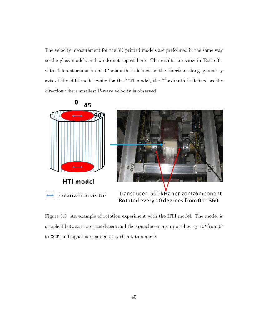
The velocity measurement for the 3D printed models are preformed in the same way

as the glass models and we do not repeat here. The results are show in Table 3.1

with different azimuth and 0° azimuth is defined as the direction along symmetry

axis of the HTI model while for the VTI model, the 0° azimuth is defined as the

direction where smallest P-wave velocity is observed.

VTI model

Transducer: 500 kHz horizontalcomponent

Rotated every 10 degrees from 0 to 360.polariza!on vector

HTI model

00 45

90

Figure 3.3: An example of rotation experiment with the HTI model. The model is

attached between two transducers and the transducers are rotated every 10° from 0°

to 360° and signal is recorded at each rotation angle.

45

HTI model VTI model

0 360 0 360

azimuth

TP

TS1

TS2

TP

TS1

TS2

180 180

!me !me

azimuth

Figure 3.4: Seismogram recorded from rotation experiments of HTI and VTI model.

Note that for HTI model, we can see clear shear-wave splitting with different azimuth

which is what we expect from HTI symmetry. For VTI model, slightly shear-wave

splitting is observed showing that the expected isotropic plane for the TI medium is

actually anisotropic indicating that the model is slightly orthorhombic.

Comparing the HTI and VTI models, we find that the HTI model follows our

assumption while the VTI model shows slightly orthorhombic symmetry. To study

why this happens, we use microscope to see its microstructure. Figure 3.5 shows the

microstructure of the 3D printed material. It’s printed layer by layer but each layer

symmetry goes perpendicular to each other. This geometry creates all-connected pore

space as we can seen from the microstructure. In this case, what we see from the VTI

azimuthal velocity is reasonable. The P-waves traveling along the two perpendicular

46

pore

space

Figure 3.5: Microstructure of the 3D printed material. It’s printed layer by layerbut each layer symmetry goes perpendicular to each other. This geometry createsconnected pore space.

directions of the fabrication symmetry in the assumed isotropic plane should have

the same velocity but faster velocity in the 45° between the two directions of the

fabrication symmetry. The fast shear wave polarized in the isotropic plane is also

influenced by the fabrication symmetry in the same way as we see from the P-wave.

However, the slow shear wave polarized perpendicular to the isotropic plane remains

almost constant compared to the fast shear wave because the fabrication symmetry

has very subtle influence. Besides azimuthal velocities, vertical velocities are also

measured and they coincide with the azimuthal velocities due to the symmetry (Table

3.2). We see that the vertical P-wave velocity of the HTI model falls in the range of

the P-wave velocity in the isotropic plane of the VTI model while the vertical P-wave

47

velocity of the VTI model is approximately the same with the P-wave velocity of the

HTI model which is normal to isotropic planes. For the shear-wave velocities, we can

find the same repeated velocities from vertical and horizontal azimuthal velocities.

Vertical velocity (m/s) VP VS‖ VS⊥

HTI 1821 884 823

VTI 1738 816 805

Table 3.2: Vertical velocity of the HTI and VTI models.

The vertical-horizontal velocity variation is about 5% while the velocity variation in

the vertical isotropic plane is about 0.8%, which making it 6 times difference. In this

case, we claim this material as major HTI symmetry, slightly orthorhombic.

3.2 Fluid substitution with printed HTI model

To study the fluid influence on velocity of an HTI medium, a fluid substitution

experiment with the HTI model is designed. The model used in this experiment is

the 3D printed HTI model. Its dry properties are measured before saturation.

3.2.1 Experiment description

The 3D printed models are anisotropic and porous making it similar to rocks. The

HTI model and the VTI model show basically the same elastic property and for

simplicity, we only study the HTI model for fluid substitution. Figure 3.6 shows the

48

air pumpwater

HTI model

vacuum

airè

Figure 3.6: Fluid substitution experiment set-up. The HTI model is put in the tankand an air pump keeps pumping air out of the tank to make it vacuum. The air inthe model is pumped out and water is sucked into the model because of capillaryforces.

experiment setup, we put the HTI model in water in a bowl. Then we put the bowl

in a sealed tank, we use an air pump to pump out the air out of the tank. Since there

is air both in water and in HTI model, the air pump keeping pumping for about one

hour until most air is pumped out. Because of the capillary force, the water is sucked

into the pore space of the HTI model. After finishing the saturation experiment, we

use tapes to wrap the HTI model to keep water from coming out and weight its mass

after saturation to know how much water there is in the model.

49

0

polariza!on

TS1

TS2

0 360

polariza!on

!me

TS1

TS2

180

!me

180

dry saturated

360

Figure 3.7: Seismogram recorded from rotation experiments of HTI model beforeand after fluid substitution experiment. An increase in shear wave travel time isobserved indicating a velocity decrease.

3.2.2 Data

The model weights 104.068 g before saturation and 107.457 g after saturation. By

subtracting the two numbers, we get the volume of water saturated in the model

as 3.389 cm3. Using the definition of porosity as volume of pore space divide

total volume, we calculate the porosity of the HTI model as 3.13%. Then we

repeat the same experiments with the dry model. Figure 3.7 shows the seismogram

recorded from rotation experiments of HTI model before and after fluid substitution

experiment. We see there is change for shear-wave splitting as the traveltime is

different now. Velocity in different directions are also measured. To help compare

the difference, velocities measured before and after saturation are shown in Table 3.3

and Table 3.4.

50

dry water-saturated

Azimuth 0° 45° 90° 0° 45° 90°

VP (m/s) 1733 1745 1806 1813 1818 1841

VS‖(m/s) 823 849 884 810 844 875

VS⊥(m/s) 823 842 823 810 838 810

Table 3.3: Velocity for different azimuth for the HTI model before and after

saturation.

Vertical velocity (m/s) VP VS‖ VS⊥

dry 1821 884 823

water-saturated 1856 874 810

Table 3.4: Vertical velocity of the HTI models before and after saturation.

3.3 Theory and method

The general equations for fluid dependency of the elastic moduli of anisotropic media

were first given by Gassmann (1951). For the case of an HTI medium, Gurevich

(2003) derived the explicit equations based on a linear-slip model. Gurevich’s

complex equations are recast here in a more accessible format. Those equations

depend on four parameters: λ, µ, ∆N and ∆T . They are quite similar to the

well-known isotropic Gassmann’s equations. We also propose a valid method for the

application of these equations.

51

3.3.1 Introduction

Fluid substitution in rocks is very important for understanding their fluid-dependent

seismic response. The most commonly used method for fluid substation comes from

the work of Gassmann (1951), which relates the bulk modulus of a rock to its porosity,

rock matrix and fluid properties. His equations (Smith et al., 2003) can be written

as:

Ksat = K +(1−K/Km)2

φ/Kfl + (1− φ)/Km −K/K2m

, (3.1)

where φ is the porosity, Ksat = the saturated bulk modulus, Km = the bulk

modulus of the mineral matrix, Kfl = the bulk modulus of the pore fluid, K =

the bulk modulus of the drained porous rock frame. Most of the applications of fluid

substitution are based on the assumption of an isotropic rock model, which may not

be quite the real case. We know that many reservoirs are fractured, and therefore

anisotropic to some extent. Actually, Gassmann (1951) also published a general

equation for anisotropic fluid substitution. His results can be written in terms of

stiffness tensors, Cijkl, where a repeated index implies a sum over 1-3 (Mavko and

Bandyopadhyay, 2009):

Csatijkl = Cijkl +

(Kmδij − Cijαα/3)(Kmδij − Cββkl/3)

(Km/Kfl)φ(Km −Kfl) + (Km − Cppqq/9), (3.2)

where,

δij =

1, i = j

0, i 6= j, (3.3)

Cppqq =3∑p=1

3∑q=1

Cppqq, (3.4)

52

Cijαα =3∑i=1

3∑j=1

3∑α=1

Cijαα, (3.5)

From Equation 3.2, we can see that to perform Gassmann’s anisotropic fluid

substitution equations, we need to know all the stiffness tensors of the rock and

we seldom have enough measurements. In this case, these equations become

useless and people have to choose isotropic equations for the anisotropic rocks

as an approximation. In order to use the anisotropic formulation, some rock

models are proposed and people derived different approximations for Gassmann’s

equations. Gurevich (2003) and Sil et al. (2011) derived the anisotropic Gassmann’s

equations for an HTI rock based on a linear-slip model (Hsu and Schoenberg, 1993;

Schoenberger and Sayers, 1995) and analyzed the effect of changing porosity and

water saturation. However, the equations they gave are difficult to understand

intuitively. Mavko and Bandyopadhyay (2009) derived an approximate fluid

substitution for vertical velocities in weakly anisotropic VTI rocks. They used the

vertical velocity to calculate the bulk modulus of ”the anisotropic material having

the same velocities as the observed vertical VTI velocities”. This calculation seems

to assume that the vertical velocity of the VTI rocks is the velocity of the isotropic

background rocks. Their approximations for the anisotropic Gassmann’s equations

are very similar to the isotropic case, but with a first-order correction proportional

to Thomsen’s parameter δ (Thomsen, 1986). They used the variation of δ to explain

why isotropic fluid substitution underpredicts or overpredicts the anisotropic results.

In our study, we derive approximations for the anisotropic Gassmann’s equations

for HTI rocks based on the linear-slip model. We use the vertical velocities as an

approximation to calculate the bulk modulus of the isotropic background (Sil, 2013).

53

The results are quite similar to the form of the isotropic case. Also, we propose

a practical method for implementing these equations and use synthetic data as an

example to test our equations.

3.3.2 HTI medium

In an HTI medium, vertical fractures are embedded along a preferred orientation

(normal to fracture planes) in an isotropic background (Figure 3.8). The fractured

rocks (or the HTI medium) can be considered as a simple combination of fractures

and isotropic rocks (Hsu and Schoenberg, 1993).

Figure 3.8: A cartoon representation of an HTI medium which consists of an isotropic

background rock and a set of oriented fractures. The symmetry axis of the medium

is normal to the fracture planes.

The isotropic rocks are characterized by Lame parameter (λ) and shear modulus

(µ) while the imbedded fractures are characterized with the dimensionless normal

54

and tangential fracture weakness, ∆N and ∆T , respectively. By using these four

parameters, we can characterize the HTI medium instead of the five independent

stiffness tensors under the constraint that (Schoenberger and Sayers, 1995):

C11C33 − C213 = 2C44(C11 + C13), (3.6)

For such an anisotropic rock model, expressions for the dry stiffness matrix can be

written as (Schoenberger and Sayers, 1995):

Cij =

C11 C13 C13 0 0 0

C13 C33 C23 0 0 0

C13 C23 C33 0 0 0

0 0 0 C44 0 0

0 0 0 0 C55 0

0 0 0 0 0 C55

=

C1 0

0 C2

, (3.7)

where 0 is the 3× 3 zero matrix and C1 and C2 are given by

C1 =

M(1−∆N) λ(1−∆N) λ(1−∆N)

λ(1−∆N) M(1− r2∆N) λ(1− r∆N)

λ(1−∆N) λ(1− r∆N) M(1− r2∆N)

, (3.8)

and

C2 =

µ 0 0

0 µ(1−∆T ) 0

0 0 µ(1−∆T )

, (3.9)

where,

M = λ+ 2µ, (3.10)

55

r = λ/(λ+ 2µ), (3.11)

∆N = ZNM/(1 + ZNM), (3.12)

∆T = ZTµ/(1 + ZTµ), (3.13)

In the equations above, ZN and ZT are the normal and tangential fracture

compliances of the anisotropic fractured rocks. With the stiffness matrix of the

dry rock, we can derive the expressions for C1α and Cpq, and substitute them into

equation 3.2, to get the explicit expressions for HTI Gassmann’s equations. Here we

take Csat11 for example.

From equation 3.2, we can write Csat11 as:

Csat11 = C11 +

(Km − C1α/3)2

(Km/Kfl)φ(Km −Kfl) + (Km − Cpq/9), (3.14)

Using equation 3.8, 3.10 and 3.11, we can express the following quantities as

C1α = 3K(1−∆N), (3.15)

Cpq = 9K(1−∆NK/M), (3.16)

where K = λ+ 2/3µ is the bulk modulus of the background isotropic rock .

Substituting equations 3.15 and 3.16 into equation 3.14, we have:

Csat11 = M(1−∆N)

+(Km −K(1−∆N))2

(Km/Kfl)φ(Km −Kfl) +Km −K + ∆NK2/M(3.17)

56

The results are very similar to the isotropic Gassmann’s equation: the first part is

the stiffness tensor of the dry rock and the second part is almost same as the isotropic

Gassmann’s equation except that we have one more term for the fractures. We can

derive other stiffness tensors of the saturated rocks in a similar way, given:

C2α = C3α = 3K(1− r∆N), (3.18)

C4α = C5α = C6α = 0, (3.19)

The results are:

Csat33 = M(1− r2∆N)

+(Km −K(1− r∆N))2

(Km/Kfl)φ(Km −Kfl) + (Km −K + ∆NK2/M)(3.20)

Csat13 = λ(1− δN)

+(Km −K(1−∆N))(Km −K(1− r∆N))

(Km/Kfl)φ(Km −Kfl) + (Km −K + ∆NK2/M)(3.21)

Csat44 = µ, (3.22)

Csat55 = µ(1−∆T ), (3.23)

By using equation 3.17 and 3.20-3.23, we can perform anisotropic fluid substitution

analysis.

3.3.3 Orthorhombic medium

Almost same derivation could be performed with orthorhombic case. Here we

consider the orthorhombic symmetry which comes from an isotropic background

57

with two vertically aligned sets of fractures orthogonal to each other. For such a

medium, Bakulin et al. (2000b) derived the effective stiffness matrix using linear slip

theory (Equation 3.24).

Cij =

C11 C12 C13 0 0 0

C12 C22 C23 0 0 0

C13 C23 C33 0 0 0

0 0 0 C44 0 0

0 0 0 0 C55 0

0 0 0 0 0 C66

=

C1 0

0 C2

, (3.24)

where 0 is the 3× 3 zero matrix and C1 and C2 are given by

C1 =1

d

Ml1m3 λl1m1 λl1m2

λl1m1 Ml3m1 λl2m1

λl1m2 λl2m1 M(l3m3 − l4)

, (3.25)

and

C2 =

µ(1−∆T2) 0 0

0 µ(1−∆T1) 0

0 0 µ (1−∆T1)(1−∆T2)

(1−∆T1∆T2)

, (3.26)

where,

l1 = 1−∆N1, (3.27)

l2 = 1− r∆N1, (3.28)

l3 = 1− r2∆N1, (3.29)

58

l4 = 4r2g2∆N1∆N2, (3.30)

m1 = 1− r2∆N2, (3.31)

m2 = 1− r∆N2, (3.32)

m3 = 1− r2∆N2, (3.33)

g = µ/(λ+ 2µ) = V 2s /V

2p , (3.34)

d = 1− r2∆N1∆N2, (3.35)

∆Ni = ZNiM/(1 + ZNiM), (3.36)

∆T i = ZT iµ/(1 + ZT iµ), (3.37)

In the equations above, ∆Ni and ∆T i (i=1,2) are the normal and tangential fracture

weakness (defined in the same way as the HTI case) of the anisotropic fractured rocks.

For such equivalence to be valid, three additional relationships should be satisfied:

C12C33 + C23 = C13(C22 + C23), (3.38)

2(C11 + C13) = (C11C33 − C213)(

C44 + C55

C44C55

−1

C66

), (3.39)

and

2(C22 + C23) = (C22C33 − C223)(

C44 + C55

C44C55

−1

C66

), (3.40)

59

With the effective stiffness matrix of the dry rock, we can derive the expressions for

C1α and Cpq, and substitute them into equation 3.2, to get the explicit expressions

for orthorhombic Gassmann’s equations. Using equations above, we can express the

following quantities (second-order terms are dropped) as

C1α = 3K(1−∆N1 − r∆N2), (3.41)

C2α = 3K(1− r∆N1 −∆N2), (3.42)

C3α = 3K(1− r∆N1 − r∆N2), (3.43)

C4α = C5α = C6α = 0, (3.44)

Cpq = 9K(1−K(∆N1 + ∆N2)

λ+ 2µ), (3.45)

By Substituting above equations into each Csatij , we have:

Csat11 = M(1−∆N1 − r2∆N2)

+(Km −K(1−∆N1 − r∆N2))2

(Km/Kfl)φ(Km −Kfl) +Km −K −K2(∆N1 + ∆N2)/M

(3.46)

Csat22 = M(1− r2∆N1 −∆N2)

+(Km −K(1− r∆N1 −∆N2))2

(Km/Kfl)φ(Km −Kfl) +Km −K −K2(∆N1 + ∆N2)/M

(3.47)

60

Csat33 = M(1− r2∆N1 − r2∆N2)

+(Km −K(1− r∆N1 − r∆N2))2

(Km/Kfl)φ(Km −Kfl) +Km −K −K2(∆N1 + ∆N2)/M

(3.48)

Csat12 = M(1−∆N1 −∆N2)

+(Km −K(1−∆N1 − r∆N2))(Km −K(1− r∆N1 −∆N2))

(Km/Kfl)φ(Km −Kfl) +Km −K −K2(∆N1 + ∆N2)/M

(3.49)

Csat13 = M(1−∆N1 −∆N2)

+(Km −K(1−∆N1 − r∆N2))(Km −K(1− r∆N1 − r∆N2))

(Km/Kfl)φ(Km −Kfl) +Km −K −K2(∆N1 + ∆N2)/M

(3.50)

Csat23 = M(1−∆N1 −∆N2)

+(Km −K(1− r∆N1 −∆N2))(Km −K(1− r∆N1 − r∆N2))

(Km/Kfl)φ(Km −Kfl) +Km −K −K2(∆N1 + ∆N2)/M

(3.51)

Csat44 = µ(1−∆T2), (3.52)

Csat55 = µ(1−∆T1), (3.53)

Csat66 = µ

(1−∆T1)(1−∆T2)

(1−∆T1∆T2), (3.54)

By using equation 3.46 to 3.54, we can perform anisotropic fluid substitution analysis

for an orthorhombic medium.

61

3.3.4 Method

Before performing the anisotropic Gassmann’s equations to an HTI medium with the

new expressions, we need to know the four parameters: λ, µ, δN and δT . There are

some assumptions: 1) The vertical P- and fast S-wave velocities of the HTI medium

are the same to the isotropic background (Sil, 2013); 2) All the pores that contribute

the porosity in our equations are interconnected; 3) The fluid diffusion length is larger

than the fracture size and spacing (Gurevich, 2003) which means the low frequency

limit; 4) The HTI medium agrees with the linear-slip model assumption. Bakulin

et al. (2000a) gave a comparison between linear-slip model and Hudson’s penny-

shaped model for the case of an HTI medium. They concluded that by satisfying

some relations, these two models could become identical and lead to the same results.

Figure 3.9 shows the work flow for parameter estimation. The vertical velocities of

the P-wave, the fast and slow S-wave, and density of the background isotropic rocks

can be obtained from a vertical well-log data. With these parameters, we can invert

for Lame parameter, λ, and shear modulus, µ, as well as C33, C44 and C55 of

the dry anisotropic rocks based on the method developed by Sil (2013). As for the

calculation of the tangential fracture compliance, ZT , the expression was given by

Hsu and Schoenberg (1993) for a VTI medium as:

ZV TIT =1

CV TI44

−1

CV TI66

, (3.55)

We know that VTI and HTI medium are equivalent in case of a 90° rotated symmetry

axis. So we can use this result and transform it from VTI to HTI medium:

ZT =1

C55

−1

C44

, (3.56)

62

Figure 3.9: Work flow for parameter estimation using well log data. Vertical velocitiesare assumed to be the background matrix velocities.

With ZT , using the relation defined by Sayers and Kachanov (1995), we can write:

ZN

ZT= 1−

ν

2, (3.57)

where ν is the background isotropic rock’s Poisson’s ratio of the background isotropic

rock which can be derived from the vertical P- and fast S-wave velocities. Generally,

obtaining the background P-wave velocity requires analysis of the unfractured core

samples. However, for practical purposes, we can consider the vertical P-wave

velocity to be equal to the background isotropic P-wave velocity (Prioul et al., 2007).

This assumption works well when the normal fracture weakness values are relatively

small. Then by substituting the values of λ, µ, ZN and ZT , we can obtain the

values of the normal and tangential fracture weakness δN and δT . Now, knowing

how to calculate the four parameters, we are ready to test the new equations. As the

63

method for the case of orthorhombic symmetry, it is much more complicated and is

not studied in this thesis as how to perform the fluid substitution.

3.3.5 Synthetic data test

The synthetic data are generated with the General Singular Approximation (GSA)

method, which can be used to calculate the effective stiffness (Shermergor, 1977).

The GSA method is applicable for a large inclusion concentration, pore connection

and arbitrary ellipsoidal shape of pores and cracks (Jiang and Chesnokov, 2012).

The friability parameter in GSA method ranges from 0 to 1, meaning pores are

all closed for 0 or all connected for 1. GSA shows good agreement with Rathore’s

synthetic sandstone measurement (Rathore et al., 1995; Bayuk and Chesnokov, 1998).

Thus, we decided to use GSA method to generate the data for testing different

HTI Gassmann algorithms. The synthetic sandstone model is based on Rathore’s

model. The friability is set to 1, which is required by the assumption of all pores

being connected in Gassmann fluid substitution (Smith et al., 2003). The synthetic

sandstone model is a two-phase model composed of matrix and cracks. The matrix is

a mixture of sand and epoxy, with bulk modulus of 5.21 GPa, shear modulus of 4.17

GPa and density of 1.712 g/cc. The cracks are penny-shaped cracks with thickness

of 0.02 mm, diameter of 1 mm and aspect ratio of 1/50. The crack density is 0.018.

Thus we can calculate the porosity of cracks which is 0.15% by using Nc = 3φ/4πχ,

here Nc is crack density, φ is porosity of cracks and χ is the aspect ratio of cracks.

The bulk moduli and densities are 0.0001 GPa, 0.0007 g/cc for gas and 2.16 GPa,

1 g/cc for water. We start with the GSA effective stiffness of the dry model and

64

input them into the exact Gassmann’s equations (Equations 3.2), the GSA method,

our HTI Gassmann approximation as well as the one from Gurevich (2003), and

then compare the output results for the four different algorithms of the saturated

synthetic model. For the dry model, C11 = 1.03 GPa; C13 = 0.30 GPa; C33 = 10.24

GPa; C44 = 4.15 GPa; C55 = 0.78 GPa. The results are shown in Figure 3.10 and

we find that our algorithm matches well with the exact Gassmann’s equations and

the GSA method. However, we should note that Gassmann’s equations assume that

shear rigidity remains constant regardless of fluid type. And in our results, the slow

shear wave velocity is determined by the tangential fracture weakness, δT , which is

approximated. In this case, our approximation might introduce variations to slow

shear wave velocity because of fluid substitution, which is different from the exact

Gassmann’s prediction. Apart from the confusions we may have from the equations,

we think that the anisotropic Gassmann’s equations are valid for predicting P-wave

velocity, but the shear wave velocity predicted by Gassmann must not be realistic.

We also study the changes in the P-wave moduli and velocities of an HTI medium

as a function of porosity and water saturation (Sw) using our equations. The model

parameters are the same with the above synthetic sandstone model. In Figure 3.11,

we plot the C11 and C33 values with increasing porosity and the water saturation is

set to 100% (top panel). We can see that the P-wave moduli decrease with increasing

porosity and C11 is more sensitive to porosity than C33.

65

Figure 3.10: Comparisons of the results from four different algorithms for thesaturated synthetic sandstone model. Top panel shows the comparison results forthe five elastic moduli. Bottom panel shows the comparison results for the P- andS-wave velocities.

66

Figure 3.11: Changes in P-wave moduli (C11 and C33) with porosity (top panel).

C11 is more sensitive to porosity change. Bottom panel shows the velocity

change with increasing porosity. Note Vp2 has a different trend compared to its

corresponding stiffness (C33). In this figure, water saturation is 100%.

67

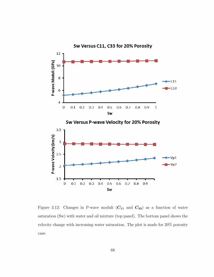
Figure 3.12: Changes in P-wave moduli (C11 and C33) as a function of water

saturation (Sw) with water and oil mixture (top panel). The bottom panel shows the

velocity change with increasing water saturation. The plot is made for 20% porosity

case.

68

In Figure 3.12 (top panel), we also plot the C11 and C33 values as a function of water

saturation with 20% porosity. The fluid here is a mixture of water and oil and the

effective fluid bulk modulus is calculated by Reuss average with the oil bulk modulus

being 1.3 GPa. As expected, P-wave moduli are increasing with water saturation and

again C11 is more sensitive than C33. However, if we look at velocity changes (Figure

3.11, bottom panel), we find that Vp2 which is the P-wave traveling parallel to the

fracture planes is decreasing with the increasing porosity. This is because when as

the porosity increases, density decreases faster than the increase of stiffness. So the

velocity increases as a result. However, for the direction normal to fracture planes,

the situation is different as the change of C11 is much greater than density. The

different trends for P-wave moduli and velocities with increasing water saturation

can be explained in a similar way (Figure 3.12). We also observe from the plots that

water saturation has a smaller influence on VP2 (or C33) as compared to porosity.

3.4 Experiment data analysis and discussion

The synthetic data test gives a good examination of the equations and now we try

to use these new equations to explain the data we get from the previous experiment.

First, we calculate the stiffness matrix of the dry (Equation 3.58) and water-saturated

(Equation 3.59) printed HTI model from measurement.

69

CHTI =

2.89 1.53 1.53 0 0 0

1.53 3.14 1.63 0 0 0

1.53 1.63 3.14 0 0 0

0 0 0 0.75 0 0

0 0 0 0 0.65 0

0 0 0 0 0 0.65

GPa (3.58)

CHTI =

3.26 1.92 1.92 0 0 0

1.92 3.42 1.90 0 0 0

1.92 1.90 3.42 0 0 0

0 0 0 0.76 0 0

0 0 0 0 0.65 0

0 0 0 0 0 0.65

GPa (3.59)

Then we use our equations (Equation 3.60) and exact Gassmann’s equations

(Equation 3.61) to predict the stiffness change after water saturation.

CHTI =

3.30 1.84 1.84 0 0 0

1.84 3.32 1.82 0 0 0

1.84 1.82 3.32 0 0 0

0 0 0 0.75 0 0

0 0 0 0 0.65 0

0 0 0 0 0 0.65

GPa (3.60)

70

Figure 3.13: Stiffness tensors from measurements and predictions. The solid-filledmarkers are predictions from our new equations and exact Gassmann’s equationswhile the unfilled markers are measured experiment data.

CHTI =

3.51 2.23 2.23 0 0 0

2.23 3.37 1.87 0 0 0

2.23 1.87 3.37 0 0 0

0 0 0 0.75 0 0

0 0 0 0 0.65 0

0 0 0 0 0 0.65

GPa (3.61)

Figure 3.13 plots the stiffness tensors from two measurements and two predictions.

The solid markers are noted as the predictions while the other two without fill are

measurements. We can see that our equations can predict the stiffness change after

water saturation well while the exact Gassmann’s equations might not work better

in this case. The velocity are also calculated (Table 3.5) and plotted (Figure 3.14)

71

Figure 3.14: Velocities from measurements and predictions. The solid-filled markersare predictions from our new equations and exact Gassmann’s equations while theunfilled markers are measured experiment data.

from the stiffness matrix.

Velocity (m/s) VP0 VP45 VP90 VS‖ VS⊥

Dry 1733 1745 1806 884 823

Measured 1813 1818 1841 875 810

Our equations 1824 1804 1831 870 810

Exact Gassmann 1882 1874 1843 870 810

Table 3.5: Velocity variation with measurements and predictions.

By comparing the velocity measurements and predictions, we find that both

predictions from our equations and the exact Gassmann’s equations match the

measured velocities. But our equations match better. This is not as expected because

72

in theory the exact Gassmann should give the best prediction. Also we find that the

exact Gassmann’s equations fail on the medium symmetry after saturation. We know

that the anisotropic symmetry should remain constant after fluid substitution can

this is confirmed by the measured data. However, the exact Gassmann’s equations

predict that after water saturation, C11 becomes bigger than C33 which is not

correct. Here is an possible explanation for this problem. The measured velocity,

especially the 45° P-wave velocity, might not be accurate enough. Yan et al. (2012)

show that the angle and velocity measurement around 45° is critical for reliable

anisotropy measurement and 1% of VP45 can cause 40% error in C13. The error

in VP45 can explain the failure of exact Gassmann which depends on the accurate

measurements of stiffness tensors. Our equations and methods, however, are free of

VP45 and thus in a sense more reliable and accurate. Also we calculate the Thomsen’s

parameters before and after fluid substitution to see how they change. Equation 2.4

to 2.6 are used for calculation and since the exact Gassmann’s equations fail, we

will not put it in further discussion. Table 3.6 shows the calculated Thomsen’s

parameters before and after saturation. From direct measurements, we see that

εV and δV decrease 41% and 39% in magnitude respectively while γV increase

8.5% in magnitude after water saturation. Our equations predict δV decreases 92%

and εV decreases 43% after saturation while γV remains constant as defined by

the equations. In summary, the 3D printed models are interesting and helpful in

understanding the fluid-dependence of anisotropic rocks. These models allow us to

examine all kinds of different theory and methods about rock physics models. In this

thesis, a new set of equations for fluid substitution for an HTI medium are derived

73

Thomsen’s parameters εV δV γV

Dry -0.039 -0.093 -0.067Measured -0.023 -0.056 -0.072

Our equations -0.003 -0.052 -0.067

Table 3.6: Thomsen’s parameters of the HTI model before and after saturation.

and tested with both synthetic data and experiment data with a printed HTI model.

The new equations work well for predicting elastic properties change with fluid.

74

Chapter 4

Conclusion

The purpose of the thesis is to characterize fracture zones through seismic data and

rock physics modeling. To do this, two physical models are studied and analyzed. A

laser-etched glass model is studied first. Ultrasonic velocity measurements help us

understand its symmetry and it turns out to be an HTI medium. Very small velocity

difference (less than 2%) between pure glass and fracture zone are observed thus

reflections from the fracture zone interfaces are expected to be subtle. Two 2D lines

which are on and off fracture zone, are surveyed for comparison and the raw data

shows the reflections from fracture zone. Some processings for signal enhancement

are done to remove linear events and to preserve and recover the true amplitude of the

reflections. By comparing the processed data from on and off fracture zone, fracture

zone reflections are confirmed. Then multi-component data are acquired with full

azimuth coverage. From all different component data, the vertical-vertical data and

horizontal-horizontal (polarised normal to survey line) data give the best signals

75

from the fracture zone. In order to recover the true amplitude of the reflections,

radiation pattern of the transducers are studied. A theoretical equation is applied to

fit the measurement and used for amplitude correction. With recovered amplitude,

AVO/AVAZ analysis is performed on the vertical-vertical component data. Through

reflection coefficient curve fitting and inversion, the azimuth is recovered. However,

because of limited offset, more sophisticated inversion for fracture paraments are

hard to perform. As for the horizontal to horizontal component data, the reflection

from the fracture zone are highly contaminated by the side reflections and its true

amplitude is not recovered with processing. However, since the azimuthal change in

amplitude of the fracture zone reflected signals are so obvious, fracture orientation

can be recovered easily with simple analysis. The converted wave signals from

the fracture zone are hard to recover from data because of some problems with

the model and transducers as discussed in Chapter 2. From the experiments with

the glass model, reflections from fracture zone are recognized with surface seismic

data. Although the reflections are very weak and contaminated with noise, careful

processing helps enhance the signals a lot. Through AVO/AVAZ analysis, the

fracture orientation is recovered. The other model studied in this thesis is a 3D

printed HTI model. This model is directly printed with a 3D printer and ultrasonic

velocity measurements show that it has an HTI symmetry but slightly orthorhombic.

For simplification, the model is studied as an HTI medium. The model is found to

be quite porous and permeable, a fluid substitution experiment is done. Elastic

properties are measured after water saturation and significant changes are observed.

There is as much as 5% increase in P-wave velocity and 2% decrease in S-wave

76

velocity. Changes in Thomsen’s parameters are even more significant. εV and

δV decrease for about 41% and 39% in magnitude respectively while γV increase

8.5% in magnitude after water saturation. To explain the changes, a new set of

equations are derived based on Gassmann’s equations and linear slip theory. The new

equations are first tested with synthetic data and they work well. Then experiment

data are analysed and explained with the new equations and the exact Gassmann’s

equations. The results show that Gassmann’s equations fail to work well because

they are quite sensitive to VP45 while our new equations which are free of VP45 work

well. However, our equations could not give a very accurate prediction for the change

of Thomsen’s parameters. The two physical models with two novel techniques give

a lot of possibilities for modeling fractured reservoirs and exhibit rich anisotropic

response. The experiments with these models help us develop and test new methods

and algorithms for fracture characterization and more progress is expected from these

models.

77

References

Bakulin, A., V. Grechka, and I. Tsvankin, 2000a, Estimation of fracture parameters

from reflection seismic data-part I: HTI model due to a single fracture set:

Geophysics, 65, 1788–1802.

——–, 2000b, Estimation of fracture parameters from reflection seismic data-part II:

Fracture models with orthorhombic symmetry: Geophysics, 65, 1803–1817.

Bayuk, I., and E. M. Chesnokov, 1998, Correlation between elastic and transport

properties of porous cracked anisotropic media: Physics and Chemistry of the

Earth, 23, 361–366.

Buddensiek, M. L., C. M. Krawczyk, N. Kukowski, and O. Oncken, 2009,

Performance of piezoelectric transducers in terms of amplitude and waveform:

Geophysics, 74, T33–T45.

Calı, J., D. A. Calian, C. Amati, R. Kleinberger, A. Steed, J. Kautz, and T. Weyrich,

2012, 3d-printing of non-assembly, articulated models: ACM Trans. Graph., 31,

130:1–130:8.

Cheadle, S. P., R. J. Brown, and D. C. Lawton, 1991, Orthorhombic anisotropy: A

physical seismic modeling study: Geophysics, 56, 1603–1613.

78

Ebrom, D. A., R. H. Tatham, K. K. Sekharan, J. A. McDonald, and G. H. F. Gardner,

1990, Hyperbolic traveltime analysis of first arrivals in an azimuthally anisotropic

medium: A physical modeling study: Geophysics, 55, 185–191.

Gassmann, F., 1951, Uber die elastizitat poroser medien: Veirteljahrsschrift der

Naturforschenden Gesellschaft, 96, 1–23.

Gurevich, B., 2003, Elastic properties of saturated porous rocks with aligned

fractures: Journal of Applied Geophysics, 54, WA157–WA166.

Hsu, C.-J., and M. Schoenberg, 1993, Elastic waves through a simulated fractured

medium: Geophysics, 58, 964–977.

Hudson, J. A., 1981, Wave speeds and attenuation of elastic waves in material

containing cracks: Geophysical Journal of the Royal Astronomical Society, 64,

no. 1, 133–150.

Jiang, T., and E. M. Chesnokov, 2012, Elastic moduli’s relation to microstructure

properties in porous media using GSA modeling: SEG Technical Program

Expanded Abstracts, 1–5.

Kuster, G., and M. Toksz, 1974, Velocity and attenuation of seismic waves in two-

phase media: Part I. theoretical formulations: Geophysics, 39, no. 5, 587–606.

Lemu, H. G., and S. Kurtovic, 2012, 3d printing for rapid manufacturing: Study

of dimensional and geometrical accuracy: IFIP Advances in Information and

Communication Technology, 384, 470–479.

Mavko, G., and K. Bandyopadhyay, 2009, Approximate fluid substitution for vertical

velocities in weakly anisotropic vti rocks: Geophysics, 74, D1–D6.

Prioul, R., A. Donald, R. Koespsell, Z. E. Marzouki, and T. Bratton, 2007, Forward

79

modeling of fracture-induced sonic anisotropy using a combination of borehole

image and sonic logs: Geophysics, 72, E135–E147.

Rathore, J. S., E. Fjaer, R. M. Holt, and L. Renlie, 1995, P- and s-wave anisotropy

of a synthetic sandstone with controlled crack geometry: Geophysical Prospecting,

43, 711–728.

Ruger, A., 2001, Reflcetion coefficients and azimuthal avo analysis in anisotropic

media: Society of Exploration Geophysicists.

Sayers, C. M., and M. Kachanov, 1995, Microcrack-induced elastic wave anisotropy

of brittle rocks: Journal of Geophysical Research, 100, 4149–4156.

Schoenberger, M., and C. M. Sayers, 1995, Seismic anisotropy of fractured rock:

Geophysics, 60, 204–211.

Segerman, H., 2012, 3d printing for mathematical visualisation: The Mathematical

Intelligencer, 34, no. 4, 56–62.

Shermergor, T. D., 1977, Theory of elasticity of inhomogeneous media, moscow:

Nanka, (in Russian).

Sil, S., 2013, Fracture parameter estimation from well-log data: Geophysics, 78,

D129–D134.

Sil, S., M. K. Sen, and B. Gurevich, 2011, Analysis of fluid substitution in a porous

and fractured medium: Geophysics, 76, 430–458.

Smith, T. M., C. H. Sondergeld, and C. S. Rai, 2003, Gassmann fluid substitutions:

A tutorial: Geophysics, 68, 430–440.

Stewart, R. R., N. Dyaur, B. Omoboya, J. J. S. de Figueiredo, M. Willis, and S. Sil,

2013, Physical modeling of anisotropic domains: Ultrasonic imaging of laser-etched

80

fractures in glass: Geophysics, 78, D11–D19.

Tatham, R. H., M. D. Matthews, K. K. Sekharan, C. J.Wade, and L. M. Liro, 1992,

A physical model study of shear-wave splitting and fracture intensity: Geophysics,

57, 647–652.

Thomsen, L., 1986, Weak elastic anisotropy: Geophysics, 51, 1954–1966.

Yan, F., D. Han, and Q. Yao, 2012, Oil shale anisotropy measurement and sensitivity

analysis: SEG Technical Program Expanded Abstracts, 1–5.

81