fluorescence spectroscopy - iss · technical note fluorescence spectroscopy yevgen povrozin and...

TECHNICAL NOTE

Fluorescence Spectroscopy

Yevgen Povrozin and Beniamino Barbieri

Published in Handbook of Measurement in Science and Engineering, vol. 3; Myer Kurtz, editor,

John Wiley & Sons, 2016. (Published on the ISS web site with permission of the Editor)

Table of Contents

1. Observables measured in fluorescence ..................................................................... 2475

2. The Perrin-Jablońsky diagram .................................................................................... 2476

3. Instrumentation ............................................................................................................ 2479 5.1 Light Source ........................................................................................................................ 2479 5.2 Monochromator ................................................................................................................... 2480 5.3 Light Detectors .................................................................................................................... 2481 5.4 Instrumentation for steady-state fluorescence: analog and photon counting ..................... 2483 5.5 The Measurement of decay times: Frequency-domain and time-domain techniques ........ 2483

6 Fluorophores ................................................................................................................ 2486

7 Measurements .............................................................................................................. 2486 7.1 Excitation spectrum ............................................................................................................. 2486 7.2 Emission spectrum .............................................................................................................. 2487 7.3 Decay times of fluorescence ............................................................................................... 2490 7.4 Quantum yield ..................................................................................................................... 2492 7.5 Anisotropy and polarization ................................................................................................. 2492

8 Conclusions ................................................................................................................. 2498

References .......................................................................................................................... 2498

Further Readings ................................................................................................................ 2499

Handbook in Science and Engineering 475

The number of fluorescence techniques applications has been continuously growing over the last 20

years. While initially intended as an analytical tool for the determination of the presence of specific

molecules in solutions, fluorescence is now routinely used in biochemistry and biophysics for studying

molecular interactions and dynamics, both in solutions and in cells; in clinical immunoassays for the

determination of the presence of specific antibodies and antigens; in drug discovery; in life sciences for

DNA sequencing; in nanotechnology and material sciences for identification and characterization of new

materials.

The reasons of the continuing increase in popularity are multiple: on one hand, it is due to the

improvements in the sensitivity of the instrumentation that allows now for the observation of single

molecules events on a routine basis; on the other hand, the interface of the instrumentation with the

personal computer has increased the automation of the data collection and the sophistication of the data

analysis. A third reason for its increased success is due to the introduction in the past thirty years of

innumerable and specific chemical probes used as markers for compounds that either do not display

fluorescence or only emit a low level of it. The extent of the applications has benefited from the

development of the Green Fluorescence Protein (GFP) family that allows for the expression of fluorescent

proteins in cells and tissues; a feature that allows the experimenter to follow the whereabouts of proteins

in live cells and even tissues in live animals.

Paradoxically, the capabilities of the instrumentation coupled to the computation power of the computer

brings new challenges to the field, as novel practitioners are not always aware of the potential pitfalls that

lie behind an experiment. In the past few years several articles and books have been published on the

subject describing in details the applications of the fluorescence techniques to the chemical and life

sciences. A brief article cannot cover such details; our goal is rather to reiterate the fundamental

principles of the technique and to mention some of the common pitfall that a user of the technique may

encounter.

1. Observables measured in fluorescence Fluorescence is generally referred to as the emission of photons from a sample following the absorption

of photons. There are other means for producing fluorescence in a sample (bioluminescence,

sonoluminescence, and electroluminescence) but in the following we will refer exclusively to the

phenomenon originated by the absorption of light.

Fluorescence is part of a general class of phenomena named luminescence; it is distinguished by the

phosphorescence as the latter takes, typically, a time of the order of one microsecond (10-6

s) or longer

while the former takes a time of the order of one nanosecond (10-9

s). As we will see in the following, the

distinction between the two is described using the more precise terminology of quantum mechanics.

Handbook in Science and Engineering Page 2476

The main five parameters measured in fluorescence spectroscopy are:

Excitation spectrum

Emission spectrum

Decay times (fluorescence lifetimes)

Quantum yield

Anisotropy (or polarization)

Recent advancements in fluorescence microscopy have introduced the measurement of additional

parameters (diffusion correlation times, brightness) but we will limit our discussion in this chapter to the

five parameters listed above and measurable using a spectrofluorometer.

The description of the fluorescence measurable parameters is best understood with the introduction of the

Perrin-Jablońsky diagram that is a quantum mechanics representation of the energy levels of a molecular

structure.

2. The Perrin-Jablońsky diagram Figure 1 is a classic representation of the electronic levels of a molecule in solution or in gas phase (in

solid phase the energy levels collapse into “bands” although the basic concepts are still valid).

The energy levels occupied by an electron are named “singlet states” and the letters 0S , 1S , 2S , ...,

indicate the ground state, the first excited state, etc.; upon absorption of a photon, an electron moves from

the ground state 0S to the excited states. Associated with each electronic level, there are several

vibrational and rotational levels, which differ in energy by a smaller amount than the corresponding

electronic levels.

Moreover, there are energy transitions that are not directly allowed (forbidden transitions). They are

identified as “triplet states” and indicated by 1T , 2T , …, etc.; they also feature associated vibrational and

rotational levels.

The absorption probability of a photon in each electronic level is described within the framework of

quantum mechanics (energy separation between the levels, momentum and spin of the various levels).

The molecules interact when in presence of photons of the appropriate photon energy E , where

cE h h

[68.1]

In the relation, h is the Planck constant (6.626 x 10-34

J s), c is the speed of light (2.9979 108 m s

-1) while

and are the frequency and wavelength of the electromagnetic wave describing the photon.


Figure 1. Perrin-Jablonsky energy diagram for a molecular structure. Singlet states are indicated

by S0, S1, ..; and triplet states by T1, T2, ..Internal conversion rate is KIC; intercrossing conversion rate between singlet and triplet states is KISC; the fluorescence decay rate is KR, while the non-fluorescence rate is KNR.

For absorption to occur, E has to be of the order of magnitude of the separation between the excited level

and the ground state; that is,

1 0S SE E E [68.2]

Let us consider a population of N molecules in a solution. Upon absorption of photons (blue lines in the

figure), a fraction of the molecules undergo a transition from the ground state 0S to the upper electronic

states, 1S , 2S ; the final state depending ultimately by the energy of the absorbed photon. The absorption

process takes an amount of time of the order of the femtosecond (10-15

s) or shorter.

Once in the excited electronic level, the molecules relax fairly rapidly (about 10-12

s) to the lowest level of

the first excited state 1S ; hence, they decay with rate Rk to emit fluorescence (green line in the figure).

The characteristic time of the fluorescence is of the order of one nanosecond (10-9

s).

There are additional decay routes that are not necessarily associated with the emission of photons; they

are indicated by ICk (internal conversion between two electronic states of the same spin multiplicity) and

ISCk (intersystem crossing conversion between the S levels and T levels). It is noteworthy to note that

the excited level 1T (triplet state) emit photons; this process is usually termed “phosphorescence” and its

characteristic time, as mentioned above, is of the order of one microsecond (10-6

s) and longer.

The Perrin-Jabloński diagram (Figure 1) is instrumental to determine the law describing the decay time of

fluorescence. If 1N is the population of the excited level 1S , upon absorption of photons the population

of the level changes are described by the relation:


1

1 1( )R NR

dNk k N f

dt [68.3]

where 1f is a function that describes the process of the excitation photons (pulsed source, continuous

wave source, etc.). By solving the equation (and disregarding 1f ), we find the

1 1(0) S

t

N N e

[68.4]

where S , the decay time of the excited state 1S is defined as:

1S

R NRk k

[68.5]

The fluorescence quantum yield is the fraction of excited molecules that return to the ground state with

the emission of fluorescence. From direct examination of the Perrin-Jablońsky diagram, one simply

divides the rate of radiative emission Rk by the total rates of deactivation, which includes both the

radiative and non-radiative contributions:

R

R NR

k

k k

[68.6]

By using the definition of decay times, the quantum yield can also be expressed in terms of lifetimes:

S

R

[68.7]

One can say that the quantum yield is the ratio of the number of emitted photons over the total number of

absorbed photons.

The five measurable parameters of fluorescence are usually used to describe these processes, namely: the

range in wavelengths of the absorption and emission of photons (excitation and emission spectra), the

orientation changes during the time the molecules are in the excited states between absorption and

emission of the photons (anisotropy or polarization), the fraction of photons emitted over the number of

photons absorbed (quantum yield) and the emission rate (decay times). After a brief overview of the

instrumentation we will examine in detail the measurement of the five parameters.


3. Instrumentation The peculiar parameters that characterize fluorescence are measured using “spectrofluorometers”;

sometimes, instruments for the measurement of excitation and emission spectra are termed

“spectrofluorimeters”, while the ones for the measurements of the decay times termed

“spectrofluorometers”. Yet, the distinction is not anymore as clearly demarked as several instruments

allow, in the same unit, to measure both the steady-state (excitation and emission spectra) and the

dynamic (decay times and rotational correlation times) properties of the fluorescence.

Usually, in all of the instruments, the fluorescence is collected at an angle of 90 degrees with respect to

the optical axis set by the excitation light beam. This geometry maximizes the efficiency of the emission

collection and reduces the background due to the excitation light.

It is worthy to mention that absorption spectra can be measured using a spectrophotometer. In this type of

instrument the light detector is placed on the same optical axis of the excitation light beam and the

instrument detects the amount of light that is being transmitted (that is, not absorbed) through the sample.

A spectrophotometer measures the difference in the intensity of two signals (typically, sample

transmittance is compared to 100% transmittance); instead, a spectrofluorometer measures a signal (the

fluorescence) over a zero background.

The key elements of a spectrofluorometer are the light source, the monochromator and the light detector.

5.1 Light Source

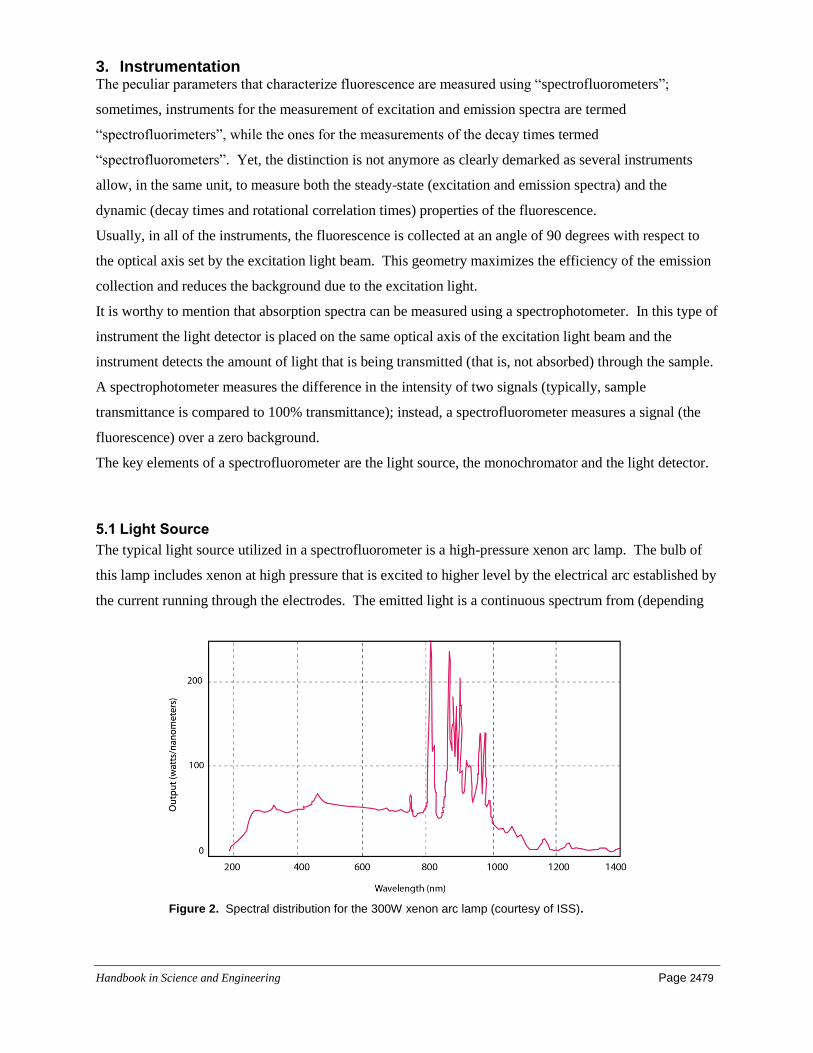
The typical light source utilized in a spectrofluorometer is a high-pressure xenon arc lamp. The bulb of

this lamp includes xenon at high pressure that is excited to higher level by the electrical arc established by

the current running through the electrodes. The emitted light is a continuous spectrum from (depending

Figure 2. Spectral distribution for the 300W xenon arc lamp (courtesy of ISS).


upon the models and geometries) about 250 nm up to 1100 nm. Figure 2 displays the spectrum of the

lamp utilized by ISS. Although the spectrum is relatively flat up to about 800 nm, several sharp

resonances are present above that wavelength.

It is worth noting that a variation of this lamp is the Hg-Xe lamp, which contains traces of mercury; this

element displays resonances at around 295 nm and this feature allowed for its use as an excitation source

for the proteins containing tryptophan.

In the past several years lasers have replaced the xenon arc lamp, specifically for time-resolved

applications. Although they emit radiation only at specific wavelengths, their brightness is order of

magnitude higher than that of the lamp. In addition, they can be pulsed with fairly narrow pulse widths

(about 50 ps for the laser diodes). A recent advancement is the supercontinuum laser (or white laser) that

delivers any wavelength in the range from 390 nm up to 2000 nm, featuring 5 ps pulsewidth and (in the

model made by Fianium Ltd) the option of selecting the repetition rate up to 40 MHz.

Light emitting diodes (LEDs) are also utilized as light sources especially in the region from 240 nm to

350 nm, where lasers are not available (with exceptions at 266 nm, 315 nm, 325 nm). They are compact,

relatively inexpensive and the source of choice when building an instrument dedicated to a specific

application.

5.2 Monochromator

Monochromators are utilized to select the wavelength used for irradiating the sample when using a xenon

arc lamp; in the collection channel of a spectrofluorometer they are utilized to record the range of

wavelengths emitted by a fluorophore (emission spectrum, see below). The simplest monochromator

includes a diffraction grating and slits at the entrance and at the output. Light impinging at an angle on

the grating is diffracted at a series of angles; usually, the first angle (or first order) is selected for the

measurement.

It is important to realize that the transmission of the light traversing a monochromator is affected by two

parameters:

1. the wavelength; the grating has a specific transmission curve and some wavelengths are

transmitted with a higher efficiency than other wavelengths, a feature to remember when

collecting excitation and emission spectra.

2. the polarization status of the radiation; the grating of the monochromator transmits differently

radiation with different planes of polarization.

Moreover, it is important to remember that when a monochromator is set to deliver radiation at

wavelength , it also delivers radiation at 2 (second order); as an example, if the excitation

monochromator is set at 300nm, it delivers radiation ad 600nm too. Typically the intensity of the second


order is about 1/10 the intensity of the first order; still this amount is sufficient to contaminate the

emission spectrum. The second order can be eliminated with a judicial selection of filters.

A characterization of every monochromator is the amount of stray light, that is radiation present at any

wavelength other than the specific wavelength the monochromator is set at. The stray light is usually

measured as the amount of light that is transmitted outside the band pass of the 632.8 nm HeNe laser line.

For typical holographic gratings it is 10-5

the intensity of the line. While this amount is not typically

important for the study of fluorophores in thin solutions, it becomes important when the sample is in a

turbid solution or even a solid state. Different strategies are available for the minimization of the stray

light, the first being a judicial selection of the grating. Gratings are classified depending upon their

fabrication process: the ruled gratings and holographic gratings, with the latter displaying less stray light

inhomogeneity as the grooves are formed through the interference process of two laser beam in a

photosensitive material, while in the former the grooves are formed mechanically.

Gratings can be arranged in different designs to build a monochromator, the two more popular being the

Czerny-Turner and the Seya-Namioka.

5.3 Light Detectors

In all the instruments the fluorescence signal is converted into current by a photomultiplier tube (PMT),

or photodiode (instruments for lifetime measurements may utilize other types of detectors too, such as

hybrid PMTs, microchannel plate detectors or streak cameras).

Figure 3 Wavelength range for a photomultiplier tube model R928 (courtesy of Hamamatsu)


Photomultiplier tubes are sensitive within a set wavelength range that is determined by the material used

in the photocathode. Figure 3 displays the region of sensitivity for the PMT Model R928 by Hamamatsu.

The PMT can be utilized in the region from about 230 nm to about 830 nm. It is apparent that even

within the operational wavelength region, the sensitivity is not the same; the non-linearity of the

sensitivity introduces an artifact in the data such that a correction to the data has to be introduced.

A spectrofluorometer includes other optical elements such as lenses and mirrors; moreover polarizers are

utilized for anisotropy measurements. The operational region of the instrument is given by the

superposition of the wavelength transmission of the various elements of the instruments. Even within this

region, the variation in transmission has to be taken into account when measuring the fluorescence

parameters. The procedures will be outlined in the measurements sections below.

Figure 4 displays the technical diagram of the K2 Multifrequency Phase Fluorometer made by ISS, an

instrument capable of measuring all of the relevant fluorescence parameters.

The standard light source is a 300 W xenon arc lamp. Continuous wave (cw) lasers, pulsed lasers

(including the multi-photon laser) and light emitting diodes (LEDs) can be coupled to the K2 as well;

typically these sources are utilized for the measurement of the decay times of fluorescence.

Figure 4. PC1 Photon Counting Spectrofluorometer (courtesy of ISS)


The light emitted by the source travels through the excitation channel that comprises the monochromator,

a filter holder and the polarizer holder; the monochromator selects the wavelength of the light that excites

the sample. The fluorescence emitted by the sample is collected through the left or the right channels; the

right channel includes the emission monochromator.

The instrument includes polarizers’ holders, filters holders, shutters for blocking the light from reaching

the sample and the detectors. All of these components are required for automated measurement

acquisition.

5.4 Instrumentation for steady-state fluorescence: analog and photon counting

Two general schemes are utilized to process the signal collected by the PMT: in one scheme, named

analog detection, the signal from the PMT goes through a current-to-voltage converter, an amplifier and,

finally, it is digitized by and analog-to-digital converter. The signal is then displayed on, and/or stored in,

the computer.

In another scheme, named photon counting detection, the signal from the PMT goes through an amplifier

discriminator that allows for the selection of pulses over a set threshold. A counter in the processing unit

counts the number of photons collected per seconds by the detector. This parameter is then displayed by

the software on, or stored in, the computer.

Although the advantage of analog detection is in the capability of processing signals within a high

dynamic range and fast response, its overall sensitivity is lower than the sensitivity of photon counting

detection. Ultimately the choice of one scheme over the other depends upon the specific application.

5.5 The Measurement of decay times: Frequency-domain and time-domain techniques

The instrumentation for the measurement of fluorescence decays times is broadly classified as belonging

to one of two groups, time-domain and frequency-domain techniques.

The time-domain technique includes the single photon counting, the multiscaler and the time correlated

single photon counting (TCSPC); the TCSPC is usually the technique utilized more often. The frequency

domain technique comes in an analog version (AFD) and a digital version (DFD) that has just been

introduced.

In TCSPC, a photon is counted within a set time period with a high precision. The time period is defined

by the intervals between the pulses of the excitation light (repetition rate of the light source) and the

precision is given by the acquisition electronics (mainly the time-to-amplitude converter (TAC) and the

analogue-to-digital converter (ADC) components). For instance, when using an excitation light, emitting

pulses at 80 MHz, the time period is the distance between two such pulses (12.5 ns). Typically, the

repetition rate of some light sources can be set by the user.


At the arrival of each pulse on the light detector, a high precision timer is triggered which records how

much time has passed between the arrival of the excitation pulse and the emitted photon.

The TAC unit produces a signal, proportional to the arrival time of the photon, different arrival times

records are grouped in different memory locations (bins) of computer memory.

To interpret the lifetime time information obtained by a TCSPC instrument a histogram of the arrival

times records is built. For a single exponential decay, a curve similar to the one of Equation [ 5] is

collected and the decay time is determined using a minimization technique to fit the experimental data

to the theoretical decay model.

Figure 5. Principle of Start-Stop mechanism utilized in TCSPC data acquisition.

The frequency domain technique is more versatile as it can perform either with pulsed sources used for

TCSPC or with the modulation of the excitation light source: the modulated excitation results in a

modulated fluorescence with a phase and modulation which is dependent on the lifetime of the excited

fluorophores.

The instruments utilized in frequency domain technique are called multifrequency phase fluorometers

(MPF) or, simply, frequency domain fluorometers. The underlying operational principle of a MPF is

illustrated by Figure 6 for a continuous wave source. The excitation light ( )E t is modulated at a

frequency ; its modulation is characterized by an alternating component EXAC and an average


component EXDC . The fluorescence light is modulated at the same frequency , but its phase is

delayed by the quantity and the overall modulation EM

ACDC

is less than the original modulation

of the excitation light. A frequency-domain instrument measures the phase shift and the demodulation

m of the fluorescence; both quantities are related to the decay time (see equations [7, 8]. For a single

exponential decay, the decay time is related to the phase angle and to the modulation by the following

relations:

1

tanP

[68.8]

2

1 11M

m

[68.9]

Such measurements are repeated at several different values of the modulation frequency, ranging

typically from two or three for a single exponential decay, to up to twenty-twenty five for multiple

exponential decays. The decay times i are determined using a minimization technique to fit the

experimental data.

Figure 6. Schematics of the excitation and emission light in frequency-

domain spectroscopy; the emission light is phase-shifted and demodulated with respect to the excitation light.


The first modern frequency-domain instrument has been introduced by Spencer and Weber in 1969. In

this instrument the light source is modulated at a frequency and the light detector is modulated at a

frequency ( ) ; the two frequencies being provided by phase-locked frequency synthesizers. The

approach is also known as “heterodyning”. The output signal includes components at the sum ( 2 ) and

the difference ( ) frequency; the low signal component , called the “cross-correlation frequency”,

which is typically in the range from 1 Hz to 20 KHz, is utilized to determine the phase shift and the

demodulation of the fluorescence. From the phase and modulation of the frequency, the phase and

the modulation of the fluorescence can be determined relative to that of a reference lifetime.

6 Fluorophores Generally fluorophores are divided into intrinsic and extrinsic. Intrinsic fluorophores are the natural

components of a system (typically biological macromolecule) that exhibit fluorescence that can be

measured; for instance the aromatic amino acids tyrosine, tryptophan and phenylalanine of the proteins,

NADH, the flavins, the porphyrins-based compounds such as chlorophylls. Extrinsic probes include all

those molecules that are foreign to the system or were added to it artificially (fluorescent probes and

labels – organic dyes, quantum dots or biological fluorophores), such as fluorescein, ANS (1,8-

anilinonaphthalene sulfonic acid), which are introduced by the experimenter. Such molecules can be

covalently linked to the molecule under study or non-covalently as is the case for DPH

(diphenylexatriene), used to study membranes.

7 Measurements

7.1 Excitation spectrum

The excitation spectrum displays the emission intensity distribution at one wavelength while scanning the

excitation wavelength over a range. Practically, for the acquisition of the excitation spectrum, the

emission monochromator of the spectrofluorometer is set at a fixed wavelength (in the sample emission

range) and the excitation monochromator is scanned over a range of wavelengths (the range that

corresponds to the sample absorption range). Referring to the Jablońsky-Perrin diagram of Figure 1,

when acquiring the excitation spectrum one detects photons emitted by the molecules at a set wavelength

(represented by one of the green lines), while scanning the wavelength of the radiation (energy of

photons) sent to the sample from high energy to low energy (blue lines).

If there are no changes occur to the molecule in the excited state, then the excitation spectrum closely

resembles the absorption spectrum acquired with a spectrophotometer, yet, in most instances, it does not:

in order for the two to match, a suitable correction of the instrumental factors has to be applied. The main


culprit of the differences is due to the lamp; it features a peculiar emission spectrum of its own, that is, the

intensity of the emitted radiation is not constant at all the wavelengths. In order to correct for this effect,

a small fraction of the excitation light is diverted in the Reference channel of the spectrofluorometer

(Figure 2) where it passes through the quantum counter and it is collected by the reference detector. The

quantum counter, usually a stable fluorophore at a high concentration in solution, delivers a number of

photons proportional to the absorbed signal; therefore, at each wavelength, we have a signal proportional

to the signal emitted by the lamp; this signal is utilized to correct the fluorescence signal collected in the

emission channel. Although this correction addresses most of the concerns, it does not completely correct

the excitation spectrum as the beam splitter utilized to divert part of the excitation light into the reference

channel reflects differently the two planes of polarization. For a full correction to be implemented, one

should place a cuvette with a scattering solution in the sample compartment and acquire an emission

spectrum over the wavelength range of interest; then acquire the emission spectrum of the fluorophore

and divide it by the spectrum of the scatterer. In this way, the excitation spectrum is fully corrected.

Practically, the correction introduced by using the quantum counter and the reference channel is

sufficient; one should nonetheless specify the experimental conditions when publishing the spectrum.

Figure 7. Excitation spectrum of Rose Bengal in a water solution, acquired using the PC1 Photon Counting Spectrofluorometer (courtesy of ISS). The spectrum was acquired by scanning the excitation monochromator from 400 nm to 600 nm in steps of 1 nm; at each position data were acquired for 1 second. The fluorescence was observed at 610 nm.

7.2 Emission spectrum

The emission spectrum of a fluorophore is most likely the most popular experimental measurement

carried out in fluorescence. The spectrum is acquired by setting the excitation wavelength at a fixed value

(one of the blue lines of Figure 1) and then by scanning the emission monochromator over a range of

emission wavelengths (the green lines of Figure 4).


There are a few general rules that apply to emission spectra:

1. The emission of fluorescence occurs at wavelengths longer than the excitation wavelength

(Stokes shift).

2. The shape of the emission spectrum does not change by changing the excitation wavelength.

3. The emission spectrum is a mirror image of the excitation spectrum of lower energy.

An examination of Figure 1 explains as to why the first rule holds. When the molecules are excited, they

relax to the lowest vibrational level of the excited states and, from there, they emit fluorescence.

Fluorescence photons have a lower energy than excitation photons (that is the fluorescence occurs at

longer wavelengths than the excitation). Hence, we also gather that the shape of the emission spectrum

does not change by changing the excitation wavelength. Finally, rule 3 establishes that the emission

spectrum ( 1 0S S transition) is a mirror image of the absorption transition involving the same levels (

0 1S S transition). If the excitation spectrum includes transitions to higher levels, the emission

spectrum will not be a mirror image of the excitation. There are exceptions to the mirror image rule: for

instance when p-terphenyl is excited the nuclei undergo a geometric rearrangement upon absorption and

the emission spectrum shows the additional vibrational structure. Excited-states reactions can also result

in emission spectra that mark a departure from the mirror rule; and so the formation of complexes (for

instance Pyrene).

As for the excitation spectrum, the emission spectrum is affected by experimental artifacts, namely, the

transmission of the emission monochromator and the sensitivity of the light detector: The transmission of

the monochromator varies with the wavelengths and, moreover, it features different transmission for the

two planes of polarization of the light (see below for the definition of light polarization); the sensitivity of

the light detector varies with the wavelength. All these variation have to be accounted for in order to

acquire a “true’ emission spectrum. To this respect, one distinguishes between technical spectrum (the

spectrum acquired by an instrument) and the corrected spectrum (the technical spectrum that has been

corrected for the experimental artifacts). Manufacturers typically provide correction files for an

instrument; these factors are embedded in the software and corrected spectra can be acquired on line; or

spectra can be corrected afterwards. Practically, one does not need to correct a spectrum unless it is

meant for publications; even in that event, it is completely acceptable to specify that the spectrum is a

technical spectrum rather than a corrected one. There are some instances when corrected spectra are

required; when calculating the quantum yield of a fluorophore one has to calculate the area under the

spectrum; the spectrum has to be corrected for providing the proper value. Another instance occurs when

using the Förster Resonance Energy Transfer (FRET), a useful tool for estimating the distances between

two interacting and close fluorophores.


Figure 8. Emission spectrum of Rose Bengal water solution, acquired using the PC1 Photon Counting Spectrofluorometer (courtesy of ISS). The excitation monochromator was set at 490 nm. The emission spectrum was acquired by scanning the emission monochromator from 500 nm to 700 nm in steps of 1 nm; at each position data were acquired for 1 second.

Besides the instrumental artifacts, the emission spectra are sometimes distorted by experimental artifacts

that a practitioner of the field needs to be aware of, namely:

1. Background fluorescence

2. The second order of the monochromator

3. The Raman spectrum of water

Background fluorescence occurs when the fluorophore is diluted in a solution and the solvent (for

example, buffer) emits some fluorescence of its own at the emission wavelength utilized in the

experiment; the resulting emission spectrum is the superposition of the individual spectra of the solvent

and the fluorophore. In this case, one can acquire the emission spectrum of the solvent alone and subtract

it from the emission spectrum of the solution in order to obtain the emission spectrum of the fluorophore.

We mentioned about the second order in the paragraph covering the monochromators: when a

monochromator is set to deliver radiation at wavelength , it also delivers radiation at 2 (second

order); although the intensity is about 1/10 of the intensity of the first order, it is sufficient to introduce

distortions when measuring turbid solutions and solid samples. The second order can be eliminated with

a judicial selection of filters.

Finally, when working with water as a solution, the Raman peaks are present at a wavelength that is 3,400

cm-1

longer than the excitation wavelength:

1 1 13,400Ex R cm [68.10]


As an example, when exciting at 300 nm an emission peak appears at 334 nm; when exciting at 350 nm,

an emission peak appears at 397 nm. Note that, while the position of the peak is fixed in unit of

wavenumbers ( 1

), the position varies when dealing in wavelengths ( ); the change in the peak

position with the change of the excitation wavelength allows for the user to discern the peak from other

peaks or artifacts. The intensity of the Raman peak provides a simple tool to verify the status of the light

source of the spectrofluorometer; measured periodically, one can have a pretty good idea of the derating

of the xenon arc lamp and make a decision as to when replace the lamp.

7.3 Decay times of fluorescence

The fact that the decay times of many fluorophores are in the range of 1 -30 ns is truly amazing as this

time scale is typical of molecular interactions in biological systems (enzyme conformational shifts,

rotational motions in proteins, photosynthetic reactions, etc.) in physiologically active systems.

The decay time is affected by many parameters of the microenvironment (temperature, ions, polarity,

viscosity, electric fields) and this is the reason it is widely utilized for studying molecular interactions.

For instance, the decay time of ANS in water is about 100 ps; when ANS is bound to a protein the

lifetime is 8-10 ns. The lifetime of ethidium bromide is 1.8ns in water; it is 22 ns when bound to DNA

and 37 ns when bound to tRNA.

Finally, the lifetimes can be used an analytical tool as well for the characterization of the presence of

specific dyes or simply for the quantitation of complex fluorescent mixtures (the type of crude oil

provided by a well, the dye in a hair spray or a soap, the production process of paper, counterfeiting of

banknotes and of drugs, etc.).

Back in 1962, Strickler and Berg published a relation to estimate a priori the excited state lifetime of a

fluorescent molecule. Yet, its usefulness is limited because of the variation of lifetimes due to the

experimental conditions. That is, the best way to know the lifetime of a fluorophores if to measure it

directly.


Figure 9. Decay curve of Anthracene in ETOH using a TCSPC instrument (ChronosBH,

by ISS).

Figure 9 displays the decay time of Anthracene in ETOH using the ChronosBH, a TCSPC instrument, by

ISS. The light source is a pulsed LED emitting at 335 nm. A high pass filter (WG 385, 50% transmission

at 385 nm) was used to separate the fluorescence. A single lifetime of 4.2 ns was determined using the

fitting routine of the software.

Figure 10. Decay curve of Anthracene in ETOH using a frequency-domain instrument

(ChronosFD, by ISS).

Figure 10 displays the decay time of Anthracene in ETOH using the ChronosFD, a frequency-domain

instrument. Phase and modulation data were acquired at fourteen different modulation frequencies

ranging from 2 MHz to about 250 MHz. The light source is a pulsed LED emitting at 370 nm. A high

pass filter (WG 389, 50% transmission at 385 nm) was used to separate the fluorescence. A single


lifetime of 4.2 ns was determined using the fitting routine of the software. In both techniques the decay

times are recovered by using a fitting algorithm (least square analysis); the algorithm the theoretical

functions that best minimize the differences with the experimental points. Other approaches are available

for the data analysis, such as the maximum entropy method (MEM) and the phasor analysis.

7.4 Quantum yield

The quantum yield is a parameter that varies widely from molecule to molecule. A few examples are

reported in Table I below. Clearly, when looking for a fluorescent probes there are advantages in

selecting one featuring a high quantum yield!

molecule wavelength range (nm)

Temperature (ºC)

solvent Quantum yield

Benzene 270-300 20 ethanol 0.04

Anthracene 360-480 20 ethanol 0.27

Tryptophan 300-380 25 H2O 0.14

Rhodamine 101 600-650 20 ethanol 1.0

Table I. Quantum yield values of selected molecules

We refer the reader to the literature listed in Further References for the measurement of the quantum

yield. We only recollect that there is a direct mode and a relative mode. The direct mode encompasses

the use of the integrating sphere, an accessory of the spectrofluorometer that allows for the determination

of the number of photons emitted by a sample. The relative mode allows for the determination of the

quantum yield of a sample by comparison to a reference of known quantum yield. Both measurements

require particular attention to the details.

7.5 Anisotropy and polarization

Anisotropy (or polarization) is a popular application of fluorescence spectroscopy as it allows for the

measurement of the rotation of molecules as well as of their shape and size and the rigidity of molecular

structures.

A light beam is described as an electromagnetic wave with an electric vector E and a magnetic vector B

perpendicular between them; both are also perpendicular to the direction of propagation of the light beam

k . Natural light can be described as the superposition of innumerable such single wave representations.


When working with natural light a particular direction of the electric vector E can be selected by using a

polarizer; such wave is said to be “polarized” (Figure 11.).

Figure 11. An unpolarized light beam traverses a polarizer; a plane of polarization is selected.

Polarized light can be utilized for interesting experiments and applications. When polarized light with the

proper energy illuminates an ensemble of molecules (Figure 12) only molecules with the excited state

dipole moment AM (or transition moment) oriented in the same direction of the electrical field

(polarization) can absorb the photons.

Figure 12. Molecules with the electric dipole

featuring a component parallel to the direction of the electric filed of the excitation light have a probability for absorption of a photon.

If the direction of polarization of the excited beam and the direction of the dipole moment of the molecule

are perpendicular to each other, no absorption takes place. In intermediate cases, the probability of the

absorption is proportional to2cos , where is the angle between the vector E of the exciting light and

the vector M of the transition moment dipole (Figure 12).

Because of the preferential absorption rules of the molecules, a polarized light introduces a photoselection

of the molecules. As the distribution of the excited fluorophores is anisotropic, the fluorescence is

anisotropic too. Any change in the direction of the transition moment AM during the time the molecule

spend in the excited level will result in a decrease of the anisotropy, that is the overall polarization of the

fluorophores solution will decrease. The decrease in the anisotropy can be due to several reasons:

no absorption

max

absorption

2cos

no absorption

max

absorption

2cos


Difference in direction between the absorption and emission transition moments. This happens as

the transitions moments of the excited states 1S and 2S may not be the same; yet, molecules emit

from the lowest vibrational level of 1S .

Brownian motion. Molecules in the excited state enter into collisions with the molecules of the

solvent or with molecules of the same species and, as a result, the direction of the emission

transition moment changes.

Energy transfer to another molecule featuring a different orientation.

Anisotropy is measured using a spectrofluorometer equipped with polarizers; one polarizer is mounted in

the excitation beam (Figure 2) and a second polarizer is inserted in the emission channel. The anisotropy

is defined as:

2

VV VH

VV VH

I gIr

I gI

[68.11]

And the polarization is

VV VH

VV VH

I gIP

I gI

[68.12]

The two parameters, anisotropy and polarization, describe the same phenomenon; they are related to each

other by

3

2

rP

r

[68.13]

(In the following description we will refer to anisotropy only). In the relations above, VVI is the

measured fluorescence intensity with the polarizer in the excitation channel in the (V)ertical position and

the polarizer in the emission channel in the (V)ertical position; VHI is the measured fluorescence intensity

with the polarizer in the excitation channel in the (V)ertical position and the polarizer in the emission

channel in the (H)orizontal position.

The number g, called the g-factor, is given by HV

HH

Ig

I , where the letters V and H refer to the positions

of the polarizers in the excitation and emission channel, respectively. The g-factor corrects the anisotropy

values for the artifact introduced by the instrument; as is the case for emission spectra, the instrument has

different transmission properties for the two planes of polarization.


Figure 13. Experimental setup for anisotropy measurements. The

spectrofluorometer has a polarizer in the excitation channel and a second polarizer in the emission channel. The intensity of the fluorescence reaching the light detector is measured for different orientation of the polarizers (see relation [ 9]).

Figure 14 displays the polarization values for Erythrosine in water along with the excitation spectrum; the

fluorescence is collected at 550nm. The polarization is negative for wavelengths below 360 nm and then

rises sharply up to 400 nm and stays almost constant above 400 nm. The reason for this behavior is due

to the fact that the excitation at the short wavelengths favors the transition 0 2S S , while at the longer

wavelengths the transition 0 1S S is the one excited: as the fluorescence is always emitted by the lowest

vibrational level of 1S , it is an indication of the different orientation of the transition moments of the

excited levels 1S and 2S . Practically, when using anisotropy measurements one has to select and specify

the excitation wavelength (and chose a wavelength displaying a high value of polarization).

Figure 14. Excitation polarization spectrum for erythosine (purple line) in

water; the excitation spectrum is represented (blue line). Fluorescence is collected at 550nm.


What are the values that the anisotropy can assume? In order to answer this question one has to introduce

the emission transition moment EM and distinguish the two cases:

(a.) EM and AM are parallel; and

(b.) EM and AM are not parallel.

Without going into the details of the calculations (the interested reader can consult one of book by Valeur

cited in the References), we note that for the case of the two moments being parallel and in absence of

any motion, it is 0 0.4r ; this value is called the fundamental anisotropy. When the two moments are

not parallel the values are confined in the range:

00.2 0.4r [68.14]

The case of the decrease of anisotropy due to Brownian motion collisions is very interesting one for its

practical applications. This is the case when molecules in the excited state rotate due to collisions with

the solvent. The amount of the depolarization depends upon the value of the decay time of the molecule,

the size of the molecule, the viscosity and temperature of the solvent. In fact, let us suppose that the

decay time is of the same order of the rotational time; it is found that the anisotropy decays, for a

spherical molecule, according to the following relation:

0( ) exp( 6 )rr t r D t [68.15]

where rD is the rotation diffusion coefficient. From the Stokes-Einstein relation 6

r

RTD

V , where V

is the hydrodynamic volume of the molecule, is the solvent viscosity, R is the gas constant and T the

absolute temperature. rD can be determined by resolving equation [13] using time-resolved fluorescence

techniques. Alternatively, if the decay is a single exponential decay, it can be solved using steady-state

technique. As:

0

1( ) exp ( / )r r t t dt

[68.16]

By direct substitution one finds

0

1 1(1 6 )rD

r r [68.17]

Handbook in Science and Engineering 97

This is the Perrin equation; it allows for the evaluation of the decay times by measurements of the steady-

state polarization! In some literature, the quantity 16C

rD , called the rotational correlation time, is

used. This case is strictly valid for a spherical molecule. When the more complex shape of a

general ellipsoid is considered, the motion is described by three rotational diffusion coefficients

associated with each of the rotational axis. The relation between the rotational correlation times

and the rotational diffusion coefficients is no longer simple. The anisotropy decay is described

by:

1 2 1 2 2(4 2 ) ( 5 ) (6 )1 2 3( ) t D D t D D t Dr t e e e [68.18]

where

1

1 2

1

(4 2 )D D

2

1 2

1

( 5 )D D

3

2

1

(6 )D

[68.19]

In this expression the quantities 1 , 2 , 3 represent expressions for the angles between the absorption

and emission dipoles and the axes of the ellipsoid; 1D and 2D are the diffusion coefficients around the

axis of symmetry and equatorial axes respectively.

There are physical conditions where a probe is restricted to motion within an angle; for instance the case

of a probe in a membrane. In these cases, the anisotropy does not decay to zero. A hindered rotator is

described by the following expression

[68.20]

Table II below lists a few applications of the technique that spans from the physical-chemistry research all

the way to clinical applications.

0( ) exp ( )cr t r r t r


spectroscopy Separation of excited states

polymers Local viscosity Molecular orientation Chain dynamics

immunology Antigen-antibody reactions Immunoassays

molecular biology

Proteins interactions Nucleic acids-proteins interactions Biological membranes Micellar systems

Table II. Selected applications of anisotropy measurements

8 Conclusions Fluorescence is a sensitive technique that, although started as an analytical tool, is used more and more

for the study of molecular interactions in-vitro and in cells; in fact, it is nowadays capable of detection of

single molecules on a routine basis. The fluorescence decay time of typical fluorophores falls in a

window (1 -20 ns) suitable for the observation of several molecular processes of biological relevance.

The spectral properties of fluorophores are changed by several processes including collisions with other

molecules, rotational diffusion, and formation of complexes; moreover, the fluorescence properties are

sensitive to changes of the environment such as pH, electrical fields, concentration, temperature, polarity.

These features have expanded the applications of fluorescence to fields as diverse as the development of

sensors for monitoring the presence of specific analytes (O2, ions) in-vitro and in-situ; to the development

of sensors for the measure of physical parameters (materials under high pressure, mechanical properties

of materials). A variety of research instruments is available for the measurement of the general and

specific parameters of the fluorescence. Dedicated instruments are utilized for the measurements in

specific immunoassays (polarimeters), in drug discovery (microwell plates and microarrays), cell sorting

(cytofluorometers), genome sequencing.

References Spencer R.D., Weber G., 1970. Measurements of subnanosecond fluorescence lifetimes with

crosscorrelation phase fluorometer. Annals New York Acad. Sci. 158, 361-376.

Strickler J.S. and Berg R.A., 1962. Relationship between absorption intensity and fluorescence lifetime

of molecules. J. Chem. Phys. 37, 814-822.


Further Readings

David M. Jameson, 2014. Introduction to Fluorescence; CRC Press – Taylor & Francis Group, Boca

Raton.

Joseph R. Lakowicz, 2006. Principles of Fluorescence Spectroscopy; 3rd

Edition, Springer–Verlag, New

York.

Bernard Valeur, 2005. Molecular Fluorescence; Wiley-VCH Verlag Gmbh, Weindheim.

Wolfgang Becker, 2005. Advanced Time-Correlated Single Photon Counting Techniques; Springer-

Verlag, Berlin/Heidelberg 2005.

fluorescence spectroscopy - iss · technical note fluorescence spectroscopy yevgen povrozin and...

Documents