fluorosim: a visual problem-solving environment for

Eurographics Workshop on Visual Computing for Biomedicine (2008)Charl Botha and Gordon Kindlmann and Wiro Niessen and Bernhard Preim (Editors)

FluoroSim: A Visual Problem-Solving Environment forFluorescence Microscopy

Cory W. Quammen1, Alvin C. Richardson1, Julian Haase2, Benjamin D. Harrison2, Russell M. Taylor II1 and Kerry S. Bloom2

1Department of Computer Science, UNC Chapel Hill, USA2Department of Biology, UNC Chapel Hill, USA

AbstractFluorescence microscopy provides a powerful method for localization of structures in biological specimens. How-ever, aspects of the image formation process such as noise and blur from the microscope’s point-spread functioncombine to produce an unintuitive image transformation on the true structure of the fluorescing molecules in thespecimen, hindering qualitative and quantitative analysis of even simple structures in unprocessed images. Weintroduce FluoroSim, an interactive fluorescence microscope simulator that can be used to train scientists whouse fluorescence microscopy to understand the artifacts that arise from the image formation process, to determinethe appropriateness of fluorescence microscopy as an imaging modality in an experiment, and to test and refinehypotheses of model specimens by comparing the output of the simulator to experimental data. FluoroSim renderssynthetic fluorescence images from arbitrary geometric models represented as triangle meshes. We describe threerendering algorithms on graphics processing units for computing the convolution of the specimen model with amicroscope’s point-spread function and report on their performance. We also discuss several cases where themicroscope simulator has been used to solve real problems in biology.

Categories and Subject Descriptors (according to ACM CCS): I.3.3 [Computer Graphics]: Picture/Image GenerationJ.3 [Life and Medical Sciences]: Biology and genetics

1. Introduction

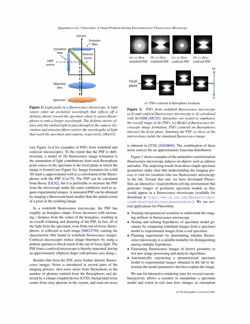
Fluorescence microscopy is an indispensable tool for imag-ing biological specimens. A traditional brightfield micro-scope records the image formed by the absorption and trans-mission of an external light source as it travels through aspecimen. In contrast, a fluorescence microscope records theimage from light emitted by fluorescing molecules, calledfluorophores, attached to or embedded within a specimen.When illuminated with light of a specific excitation fre-quency, these molecules fluoresce, emitting light at a lowerfrequency. A dichroic mirror filters out the excitation fre-quency, allowing only the light at the fluorescence frequencyto be registered by the image sensor. Figure 1 shows a con-ventional fluorescence microscope setup.

Fluorescence microscopy has three key benefits. Scien-tists can label only the parts of the specimen in which theyare interested with fluorophores, making tasks such as de-termining the location and structure of specific subcellularcomponents much easier than with conventional bright field

microscopy. Additionally, fluorescence microscopy enablesin vivo experiments impossible with other higher resolutionimaging modalities that require conditions fatal to the speci-men, such as the vacuum required in a transmission electronmicroscope. Finally, fluorescence microscopy allows opticalsectioning of specimens by adjusting the focal plane througha series of positions along the optical axis (conventionallydenoted as the z-axis), forming a stack of 2D images thatconstitutes a 3D image of the specimen.

While the benefits of fluorescence microscopy have pro-pelled it into widespread use in microbiological research,artifacts from the image formation process pose challengesfor qualitative and quantitative analysis. A 3D point-spreadfunction (PSF) characterizes the optical response of a fluo-rescence microscope to a point source of light. The PSF canbe thought of as a blurring kernel, producing the fuzzy im-ages characteristic of fluorescence microscopy. An xy-slicein the PSF represents how light passes from a point sourceemitter through the focal plane associated with that slice

c© The Eurographics Association 2008.

Quammen et al. / FluoroSim: A Visual Problem-Solving Environment for Fluorescence Microscopy

!"#$%&'()*

+,%-.*

!/$00$()*

+,%-.*

1$#2.($#*

/$..(.*3$42%*

0(5.#-*

678-#'9-*

,-)0*

:;-#$/-)*

<&/-.&*

Figure 1: Light paths in a fluorescence microscope. A lightsource emits an excitation wavelength that reflects off adichroic mirror toward the specimen where it causes fluoro-phores to emit a longer wavelength. The dichroic mirror al-lows only the emitted light to pass through to the camera. Ex-citation and emission filters restrict the wavelengths of lightthat reach the specimen and camera, respectively [Mur01].

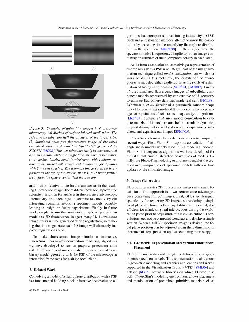
(see Figure 2a-d for examples of PSFs from widefield andconfocal microscopes). To the extent that the PSF is shift-invariant, a model of 2D fluorescence image formation isthe summation of light contributions from each fluorophorepoint source in the specimen to the focal plane at which theimage is formed (see Figure 2e). Image formation for a full3D stack is approximated well as a convolution of the fluoro-phores with the PSF [Cas79]. The PSF can be calculatedfrom theory [GL92], but it is preferable to measure the PSFfrom the microscope under the same conditions used to ac-quire experimental images. A measured PSF can be obtainedby imaging a fluorescent bead smaller than the spatial extentof a pixel in the resulting image.

In a widefield fluorescence microscope, the PSF hasroughly an hourglass shape. Focus decreases with increas-ing z distance from the center of the hourglass, resulting inan overall widening and dimming of the PSF. In fact, all ofthe light from the specimen, even from out-of-focus fluoro-phores, is collected in each image [MKCC99], causing thecharacteristic blur found in widefield fluorescence images.Confocal microscopes reduce image blurriness by using apinhole aperture to block much of the out-of-focus light. ThePSF from a confocal microscope is thereby truncated, havingan approximately elliptical shape with primary axis along z.

Besides blur from the PSF, noise further distorts fluores-cence images. Noise is introduced in several parts of theimaging process: shot noise arises from fluctuations in thenumber of photons emitted from the fluorophores and de-tected by a charge-coupled device (CCD), background noisecomes from stray photons in the system, and read-out noise

(a) xy-slice,widefield PSF

(b) xz-slice,widefield PSF

(c) xy-slice,confocal PSF

(d) xz-slice,confocal PSF

!"#$%&

'%$()&

*!&

+!&

(e) PSFs centered at fluorophore locations

Figure 2: PSFs from widefield fluorescence microscope(a-b) and confocal fluorescence microscope (c-d) calculatedwith XCOSM [MC02]. Intensities are scaled to emphasizethe overall shape of the PSFs. (e) Model of fluorescence mi-croscope image formation. PSFs centered on fluorophoresintersect the focal plane. Summing the PSF xy-slices at theintersections yields the simulated fluorescence image.

is inherent in CCDs [SGGR06]. The combination of thesenoise sources fits an approximately Gaussian distribution.

Figure 3 shows examples of the unintuitive transformationfluorescence microscopy induces on objects such as spheresand tubes. The surprising results from these simple specimengeometries make clear that understanding the imaging pro-cess is vital for scientists who use fluorescence microscopyin the lab. Toward that end, we have developed Fluoro-Sim, an interactive visual problem-solving environment thatgenerates images of geometric specimen models as theywould appear in a fluorescence microscope (available fordownload at http://www.cs.unc.edu/Research/nano/cismm/download/microscopesimulator/). We see sev-eral applications for FluoroSim:

• Training inexperienced scientists to understand the imag-ing artifacts in fluorescence microscopy.

• Testing and refining hypotheses of specimen model ge-ometry by comparing simulated images from a specimenmodel to experimental images from a real specimen.

• Planning experiments by determining whether fluores-cence microscopy is a suitable modality for distinguishingamong multiple hypotheses.

• Generating fluorescence images of known geometry totest new image processing and analysis algorithms.

• Automatically registering a parameterized specimenmodel to experimental images obtained in the lab to de-termine the model parameters that best explain the image.

We aim for interactive rendering rates for several reasons.Interactivity allows a scientist to manipulate a specimenmodel and watch in real time how changes in orientation


http://www.cs.unc.edu/Research/nano/cismm/download/microscopesimulator/

http://www.cs.unc.edu/Research/nano/cismm/download/microscopesimulator/


(a) (b)

(c)

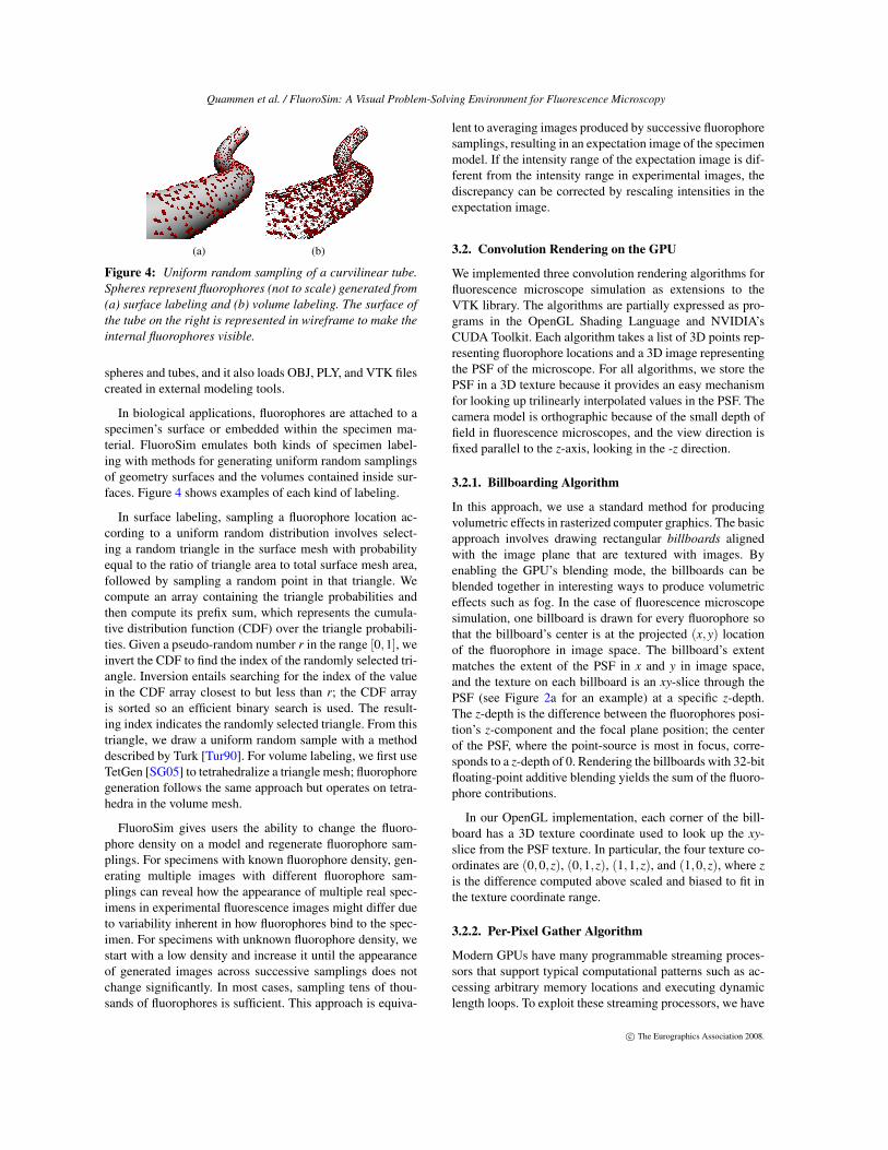
Figure 3: Examples of unintuitive images in fluorescencemicroscopy. (a) Models of surface-labeled small tubes. Theside-by-side tubes are half the diameter of the larger tube.(b) Simulated noise-free fluorescence image of the tubesconvolved with a calculated widefield PSF generated byXCOSM [MC02]. The two tubes can easily be misconstruedas a single tube while the single tube appears as two tubes.(c) A surface-labeled bead (in wireframe) with 1 micron ra-dius superimposed with experimental images at focal planeswith 2 micron spacing. The top-most image could be inter-pretted as the top of the sphere, but it is four times furtheraway from the sphere center than the true top.

and position relative to the focal plane appear in the result-ing fluorescence image. The real-time feedback improves thescientist’s intuition for artifacts in fluorescence microscopy.Interactivity also encourages a scientist to quickly try outinteresting scenarios involving specimen models, possiblyleading to insight on future experiments. Finally, in futurework, we plan to use the simulator for registering specimenmodels to 3D fluorescence images; many 3D fluorescenceimage stacks will be generated during registration, so reduc-ing the time to generate each 2D image will ultimately im-prove registration speed.

To make fluorescence image simulation interactive,FluoroSim incorporates convolution rendering algorithmswe have developed to run on graphics processing units(GPUs). These algorithms compute the convolution of an ar-bitrary model geometry with the PSF of the microscope atinteractive frame rates for a single focal plane.

2. Related Work

Convolving a model of a fluorophore distribution with a PSFis a fundamental building block in iterative deconvolution al-

gorithms that attempt to remove blurring induced by the PSF.Such image restoration methods attempt to invert the convo-lution by searching for the underlying fluorophore distribu-tion in the specimen [MKCC99]. In these algorithms, thespecimen model is represented implicitly by an image con-taining an estimate of the fluorophore density in each voxel.

Aside from deconvolution, convolving a representation offluorophores with a PSF is an integral part of the image sim-ulation technique called model convolution, on which ourwork builds. In this technique, the distribution of fluoro-phores is modeled either explicitly or as the result of a sim-ulation of biological processes [SGP∗04] [GOB07]. Fink etal. used simulated fluorescence images of subcellular com-ponent models represented by constructive solid geometryto estimate fluorophore densities inside real cells [FML98].Lehmussola et al. developed a parametric random shapemodel for generating simulated fluorescence microscope im-ages of populations of cells to test image analysis algorithms[LRS∗07]. Sprague et al. used model convolution to eval-uate models of kinetochore-attached microtubule dynamicsin yeast during metaphase by statistical comparison of sim-ulated and experimental images [SPM∗03].

FluoroSim advances the model convolution technique inseveral ways. First, FluoroSim supports convolution of tri-angle mesh models widely used in 3D modeling. Second,FluoroSim incorporates algorithms we have developed forthe GPU that enable interactive convolution of models. Fi-nally, the FluoroSim modeling environment enables the cre-ation and manipulation of specimen models with real-timeupdates of the simulated image.

3. Image Generation

FluoroSim generates 2D fluorescence images at a single fo-cal plane. This approach has two performance advantagesover generating full 3D images. First, GPUs are designedspecifically for rendering 2D images, so rendering a singlefocal plane at a time fits their capabilities well. Second, it isefficient for mimicking real microscopes during the explo-ration phase prior to acquisition of a stack; an entire 3D con-volution need not be computed to extract and display a singlesection. When a full 3D specimen image is desired, the fo-cal plane position can be adjusted along the z-dimension inincremental steps just as in optical sectioning microscopy.

3.1. Geometric Representation and Virtual FluorophorePlacement

FluoroSim uses a standard triangle mesh for representing ge-ometric specimen models. This representation is ubiquitousin geometric modeling and graphics applications and is wellsupported in the Visualization Toolkit (VTK) [SML06] andTetGen [SG05], software libraries on which FluoroSim isbuilt. FluoroSim’s modeling environment allows placementand manipulation of predefined primitive models such as



(a) (b)

Figure 4: Uniform random sampling of a curvilinear tube.Spheres represent fluorophores (not to scale) generated from(a) surface labeling and (b) volume labeling. The surface ofthe tube on the right is represented in wireframe to make theinternal fluorophores visible.

spheres and tubes, and it also loads OBJ, PLY, and VTK filescreated in external modeling tools.

In biological applications, fluorophores are attached to aspecimen’s surface or embedded within the specimen ma-terial. FluoroSim emulates both kinds of specimen label-ing with methods for generating uniform random samplingsof geometry surfaces and the volumes contained inside sur-faces. Figure 4 shows examples of each kind of labeling.

In surface labeling, sampling a fluorophore location ac-cording to a uniform random distribution involves select-ing a random triangle in the surface mesh with probabilityequal to the ratio of triangle area to total surface mesh area,followed by sampling a random point in that triangle. Wecompute an array containing the triangle probabilities andthen compute its prefix sum, which represents the cumula-tive distribution function (CDF) over the triangle probabili-ties. Given a pseudo-random number r in the range [0,1], weinvert the CDF to find the index of the randomly selected tri-angle. Inversion entails searching for the index of the valuein the CDF array closest to but less than r; the CDF arrayis sorted so an efficient binary search is used. The result-ing index indicates the randomly selected triangle. From thistriangle, we draw a uniform random sample with a methoddescribed by Turk [Tur90]. For volume labeling, we first useTetGen [SG05] to tetrahedralize a triangle mesh; fluorophoregeneration follows the same approach but operates on tetra-hedra in the volume mesh.

FluoroSim gives users the ability to change the fluoro-phore density on a model and regenerate fluorophore sam-plings. For specimens with known fluorophore density, gen-erating multiple images with different fluorophore sam-plings can reveal how the appearance of multiple real spec-imens in experimental fluorescence images might differ dueto variability inherent in how fluorophores bind to the spec-imen. For specimens with unknown fluorophore density, westart with a low density and increase it until the appearanceof generated images across successive samplings does notchange significantly. In most cases, sampling tens of thou-sands of fluorophores is sufficient. This approach is equiva-

lent to averaging images produced by successive fluorophoresamplings, resulting in an expectation image of the specimenmodel. If the intensity range of the expectation image is dif-ferent from the intensity range in experimental images, thediscrepancy can be corrected by rescaling intensities in theexpectation image.

3.2. Convolution Rendering on the GPU

We implemented three convolution rendering algorithms forfluorescence microscope simulation as extensions to theVTK library. The algorithms are partially expressed as pro-grams in the OpenGL Shading Language and NVIDIA’sCUDA Toolkit. Each algorithm takes a list of 3D points rep-resenting fluorophore locations and a 3D image representingthe PSF of the microscope. For all algorithms, we store thePSF in a 3D texture because it provides an easy mechanismfor looking up trilinearly interpolated values in the PSF. Thecamera model is orthographic because of the small depth offield in fluorescence microscopes, and the view direction isfixed parallel to the z-axis, looking in the -z direction.

3.2.1. Billboarding Algorithm

In this approach, we use a standard method for producingvolumetric effects in rasterized computer graphics. The basicapproach involves drawing rectangular billboards alignedwith the image plane that are textured with images. Byenabling the GPU’s blending mode, the billboards can beblended together in interesting ways to produce volumetriceffects such as fog. In the case of fluorescence microscopesimulation, one billboard is drawn for every fluorophore sothat the billboard’s center is at the projected (x,y) locationof the fluorophore in image space. The billboard’s extentmatches the extent of the PSF in x and y in image space,and the texture on each billboard is an xy-slice through thePSF (see Figure 2a for an example) at a specific z-depth.The z-depth is the difference between the fluorophores posi-tion’s z-component and the focal plane position; the centerof the PSF, where the point-source is most in focus, corre-sponds to a z-depth of 0. Rendering the billboards with 32-bitfloating-point additive blending yields the sum of the fluoro-phore contributions.

In our OpenGL implementation, each corner of the bill-board has a 3D texture coordinate used to look up the xy-slice from the PSF texture. In particular, the four texture co-ordinates are (0,0,z), (0,1,z), (1,1,z), and (1,0,z), where zis the difference computed above scaled and biased to fit inthe texture coordinate range.

3.2.2. Per-Pixel Gather Algorithm

Modern GPUs have many programmable streaming proces-sors that support typical computational patterns such as ac-cessing arbitrary memory locations and executing dynamiclength loops. To exploit these streaming processors, we have



implemented a fragment program that, for every pixel in theoutput image, iterates through the list of fluorophore loca-tions and sums the light contribution from each fluorophoreto the pixel.

A fluorophore’s contribution to a pixel is determined bycomputing a 3D offset from the fluorophore location to thepixel center in world space and using that vector, after ap-propriate scaling and biasing, as an index into the 3D PSFtexture. The value returned by the texture lookup is com-puted by hardware-accelerated trilinear interpolation of theeight PSF voxels that surround the center of the image pixel.Fluorophores falling outside the boundary of the PSF cen-tered at the pixel contribute no light to the pixel.

There are some implementation challenges with this ap-proach. We store the list of fluorophore locations as a 32-bitfloating-point RGB texture on the GPU where the red, green,and blue components correspond to x, y, and z components,respectively. While a 1D texture provides a natural way tostore a list of points, each texture dimension is limited toonly several thousand texture elements. Because potentiallymillions of fluorophores may be generated from a specimenmodel, we store the 3D fluorophore locations in a 2D textureand add appropriate 2D indexing calculations to the frag-ment program. Furthermore, on older GPUs, the number ofinstructions that can be executed is finite, limiting the num-ber of fluorophores that can be processed in one fragmentprogram invocation. Our solution is a multi-pass approachwhere each pass gathers the light contributions from a sub-set of the fluorophores and adds the results to the framebufferwith additive blending.

Two optimizations increase the speed of this algorithm.In the first optimization, a screen-space bounding rectangleof the projected fluorophores dilated by a rectangle half thescreen-space extent of the PSF limits the computation do-main. The bounding rectangle is large enough to ensure thatall pixels potentially having fluorophore contributions areprocessed while excluding pixels that cannot receive contri-butions from fluorophores. The second optimization comesfrom considering that fluorophores on a specimen modelare likely to be close together while specimen models maybe far apart. A multi-pass approach is used where a sepa-rate bounding rectangle is computed and processed for eachspecimen model. This optimization potentially reduces thetotal number of pixels covered by the bounding rectangles,particularly for small specimens separated by large distancesin the rendered image. It also reduces the ratio of fluoro-phores that contribute to a pixel to those that do not becausefluorophores far from the pixel are not examined in the frag-ment program.

3.2.3. Fourier Domain Algorithm

The previous two convolution methods operate in the spatialdomain. Using the Fast Fourier Transform (FFT), convolu-tion via point-wise multiplication in the Fourier domain is

asymptotically faster than the spatial domain methods. Wehave implemented a Fourier domain based algorithm thatbins fluorophores into an image, then convolves that imagewith the PSF. Rather than compute a full 3D convolution,we follow Sprague et al. and implement a method that sumstogether partial 2D convolutions of subsets of the fluoro-phores to produce a 2D image at a particular focal planedepth [SPM∗03]. The algorithm proceeds as follows:

1. With additive blending enabled, rasterize as points thefluorophores within a thin slab normal to the z-axis into afluorophore image.

2. Render the PSF slice corresponding to the slab into a sec-ond image.

3. Convolve the two images using the FFT algorithm andcomponent-wise multiplication in the Fourier domain.

4. Add the convolution result to an accumulation image.5. Repeat for all slabs in z within the z-extent of the PSF.

On the GPU we compute Step 1 by adjusting camera clip-ping planes and rendering all the fluorophores into a texturetarget with additive floating-point blending. A slab thick-ness 0.25 times the z-spacing of the PSF offers a tradeoffbetween accuracy and speed; a smaller fraction of the z-spacing would produce more accurate results at the cost ofcomputing the convolution of more slabs. We compute Step2 by rendering the PSF into a second texture target, cycli-cally shifting the PSF slice so that its center is at the imageorigin. As in the billboarding algorithm, the PSF slice is de-termined by converting the world space difference betweenthe slab and the focal plane into the third coordinate of the3D PSF texture lookup. Step 3 makes use of the CUFFT li-brary function that computes the FFT on the GPU as wellas a custom CUDA kernel function for computing the point-wise multiplication in the Fourier domain. Finally, Step 4 iscomputed by rendering the convolution result into an accu-mulation texture with additive blending.

When specimen models are small relative to the extent ofthe PSF in the z-dimension, many of the slabs will containno fluorophores and hence there is no need to compute theconvolution. To prevent unnecessary computation, we checkhow many fluorophores were rendered into the slab imagewith OpenGL occlusion queries. If none are rendered, wecan skip the convolution for that slab.

Because rasterizing the fluorophores quantizes the fluoro-phore locations, the method is less accurate than the two spa-tial domain methods. To increase accuracy, thinner slabs andhigher resolution of the fluorophore and PSF images couldbe used at the cost of increased memory and computation.

3.3. Gaussian Noise Generation

To indicate expected variability due to noise in fluorescenceimages, we implemented Gaussian noise generation on theGPU. We generate uniform random numbers in parallel us-ing the method described in [TW08]. For each pixel, two



# fluoro-phores

Billboardingalgorithm

Gatheralgorithm

Fourier al-gorithm

64 × 64 image of a single specimen50,000 242.1 112.0 125.7100,000 483.5 217.5 133.2200,000 964.8 429.5 146.7400,000 1,932.0 852.9 174.3800,000 3,857.8 1,711.5 231.4

512 × 512 image of a single specimen50,000 1,307.3 499.5 1,398.9100,000 2,613.6 993.4 1,404.4200,000 5,226.0 1,982.0 1,428.2400,000 10,452.6 3,976.6 1,445.6800,000 failed 7,949.0 1,503.7

512 × 512 image of three specimens separated in z50,000 1,307.2 505.3 4,092.2100,000 2,617.1 1,000.1 4,131.7200,000 5,230.6 1,985.6 4,170.4400,000 10,458.8 3,961.5 4,182.5800,000 failed 7,894.6 4,299.7

Table 1: Rendering times (in milliseconds) of the three con-volution algorithms as a function of fluorophore count.

of the four 32-bit pseudo-random numbers generated withthis method are used to generate a sample from a normal-ized Gaussian distribution using the Box-Muller transform[BM58]. The generated noise is added to the image follow-ing the convolution rendering step.

4. Performance Results

We tested the performance of the three convolution render-ing algorithms under three modeling scenarios:

• Rendering an image of a single small specimen modelwhere the spatial extent of the image is small relative tothe spatial extent of the PSF image.

• Rendering an image of a single small specimen modelwhere the spatial extent of the image is large relative tothe spatial extent of the PSF image.

• Rendering a large image of three small specimens sepa-rated in x and y by distances greater than the spatial extentof the PSF and separated by one micron in z.

The specimen models were surface-labeled one micronspheres, the PSF was 150× 150× 41 pixels with pixel size65×65×100nm, and spatial extent of the rendered 2D im-age pixels was 65× 65nm. Noise generation was disabled.All tests were run on a PC with an Intel 2.33 GHz Core 2Duo processor, 4 GB RAM, and a single NVIDIA GeForce8800 GTX GPU.

Table 1 shows timings for the three scenarios with mod-els labeled by different numbers of fluorophores. In all tests,the per-pixel gather algorithm is over twice as fast as the

billboarding algorithm. For 800,000 fluorophores, the bill-boarding algorithm failed to compute the 512× 512 imagesbecause it exceeded a time limit imposed by the GPU driver.The Fourier domain algorithm is generally slower than theother algorithms for small numbers of fluorophores but isfaster when the number of fluorophores is sufficiently high.Finally, the Fourier algorithm run-time is determined primar-ily by the size of the rendered image and the number of slabconvolutions computed; it grows slowly as the number offluorophores increases.

The billboarding approach is optimal for minimizing thenumber of additions performed on the GPU because everypixel affected by a fluorophore is touched exactly once whencomputing the contribution of that fluorophore. The per-pixel gather method is potentially suboptimal because everypixel in the screen-space bounding rectangle is touched byeach fluorophore regardless of whether it contributes to thepixel. However, the GPU on which we have tested Fluoro-Sim has fewer raster units than shading processors and theyoperate at a lower clock frequency, significantly reducing therate at which the additive blending used in the billboardingmethod can be performed. This explains the lower perfor-mance of billboarding algorithm compared to the per-pixelgather algorithm.

5. Applications

We have used FluoroSim to answer questions in several real-world applications. All images in these applications weregenerated by the per-pixel gather algorithm with no Gaus-sian noise. In all applications, we used the same PSF whichwas calculated by XCOSM [MC02] with the microscope pa-rameters used to take the experimental images in Figures 5cand 5e.

Is a model of the mitotic spindle in yeast plausible?

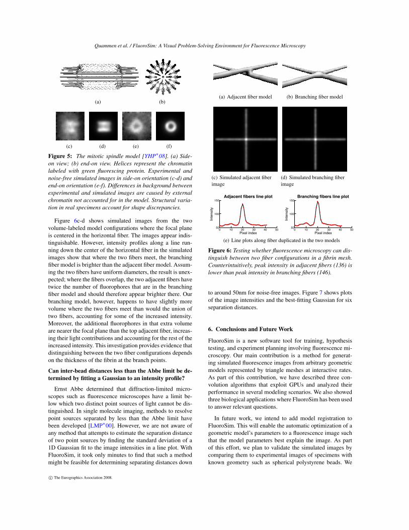
During cell division, the mitotic spindle is a structure thatensures both the mother and daughter cells receive a copyof the DNA. We created a model of the mitotic spindle in S.cerevisiae featuring a hypothesized cylindrical arrangementof chromatin surrounding interpolar microtubules that formthe backbone of the spindle apparatus [YHP∗08]. Our col-laborators (authors Haase and Bloom) take the qualitativematch of the simulated and experimental images (see Figure5) as evidence that supports the model.

Can fluorescence microscopy distinguish betweenbranching and adjacent fibrin fibers?

Fibrin is a polymerized protein that forms into a mesh inblood clots. A challenge in understanding the structure offibrin meshes and their mechanical properties is distinguish-ing between fibers that branch and fibers that are merely ad-jacent to each other. We used FluoroSim to create modelsof both configurations to determine whether a fluorescencemicroscope with this PSF can distinguish between them.



(a) (b)

(c) (d) (e) (f)

Figure 5: The mitotic spindle model [YHP∗08]. (a) Side-on view; (b) end-on view. Helices represent the chromatinlabeled with green fluorescing protein. Experimental andnoise-free simulated images in side-on orientation (c-d) andend-on orientation (e-f). Differences in background betweenexperimental and simulated images are caused by externalchromatin not accounted for in the model. Structural varia-tion in real specimens account for shape discrepancies.

Figure 6c-d shows simulated images from the twovolume-labeled model configurations where the focal planeis centered in the horizontal fiber. The images appear indis-tinguishable. However, intensity profiles along a line run-ning down the center of the horizontal fiber in the simulatedimages show that where the two fibers meet, the branchingfiber model is brighter than the adjacent fiber model. Assum-ing the two fibers have uniform diameters, the result is unex-pected; where the fibers overlap, the two adjacent fibers havetwice the number of fluorophores that are in the branchingfiber model and should therefore appear brighter there. Ourbranching model, however, happens to have slightly morevolume where the two fibers meet than would the union oftwo fibers, accounting for some of the increased intensity.Moreover, the additional fluorophores in that extra volumeare nearer the focal plane than the top adjacent fiber, increas-ing their light contributions and accounting for the rest of theincreased intensity. This investigation provides evidence thatdistinguishing between the two fiber configurations dependson the thickness of the fibrin at the branch points.

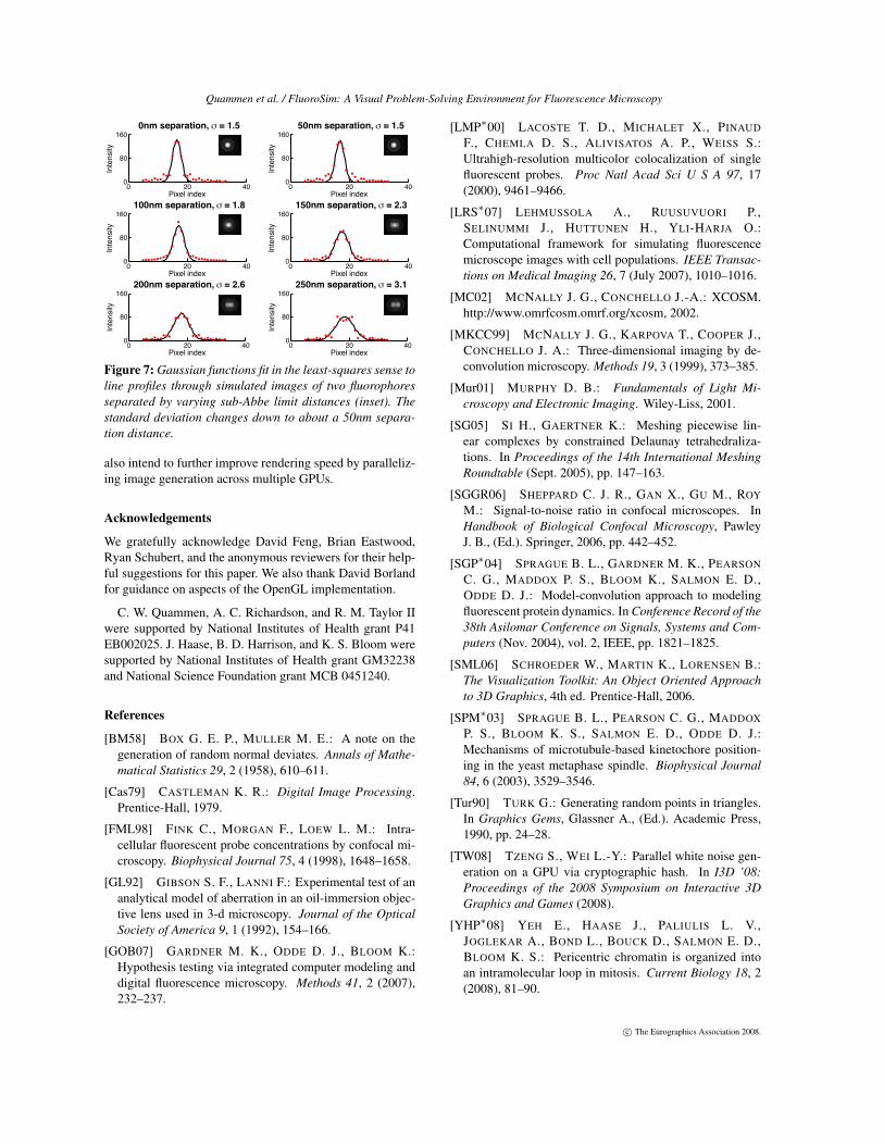
Can inter-bead distances less than the Abbe limit be de-termined by fitting a Gaussian to an intensity profile?

Ernst Abbe determined that diffraction-limited micro-scopes such as fluorescence microscopes have a limit be-low which two distinct point sources of light cannot be dis-tinguished. In single molecule imaging, methods to resolvepoint sources separated by less than the Abbe limit havebeen developed [LMP∗00]. However, we are not aware ofany method that attempts to estimate the separation distanceof two point sources by finding the standard deviation of a1D Gaussian fit to the image intensities in a line plot. WithFluoroSim, it took only minutes to find that such a methodmight be feasible for determining separating distances down

(a) Adjacent fiber model (b) Branching fiber model

(c) Simulated adjacent fiberimage

(d) Simulated branching fiberimage

0 10 20 30 40 5050

100

150Adjacent fibers line plot

Pixel index

Inte

nsity

0 10 20 30 40 5050

100

150Branching fibers line plot

Pixel index

Inte

nsity

(e) Line plots along fiber duplicated in the two models

Figure 6: Testing whether fluorescence microscopy can dis-tinguish between two fiber configurations in a fibrin mesh.Counterintuitively, peak intensity in adjacent fibers (136) islower than peak intensity in branching fibers (146).

to around 50nm for noise-free images. Figure 7 shows plotsof the image intensities and the best-fitting Gaussian for sixseparation distances.

6. Conclusions and Future Work

FluoroSim is a new software tool for training, hypothesistesting, and experiment planning involving fluorescence mi-croscopy. Our main contribution is a method for generat-ing simulated fluorescence images from arbitrary geometricmodels represented by triangle meshes at interactive rates.As part of this contribution, we have described three con-volution algorithms that exploit GPUs and analyzed theirperformance in several modeling scenarios. We also showedthree biological applications where FluoroSim has been usedto answer relevant questions.

In future work, we intend to add model registration toFluoroSim. This will enable the automatic optimization of ageometric model’s parameters to a fluorescence image suchthat the model parameters best explain the image. As partof this effort, we plan to validate the simulated images bycomparing them to experimental images of specimens withknown geometry such as spherical polystyrene beads. We



0 20 400

80

160

0nm separation, ! = 1.5

Pixel index

Inte

nsity

0 20 400

80

160


Pixel index

Inte

nsity

0 20 400

80

160


Pixel index

Inte

nsity

0 20 400

80

160


Pixel indexIn

ten

sity

0 20 400

80

160


Pixel index

Inte

nsity

0 20 400

80

160


Pixel index

Inte

nsity

Figure 7: Gaussian functions fit in the least-squares sense toline profiles through simulated images of two fluorophoresseparated by varying sub-Abbe limit distances (inset). Thestandard deviation changes down to about a 50nm separa-tion distance.

also intend to further improve rendering speed by paralleliz-ing image generation across multiple GPUs.

Acknowledgements

We gratefully acknowledge David Feng, Brian Eastwood,Ryan Schubert, and the anonymous reviewers for their help-ful suggestions for this paper. We also thank David Borlandfor guidance on aspects of the OpenGL implementation.

C. W. Quammen, A. C. Richardson, and R. M. Taylor IIwere supported by National Institutes of Health grant P41EB002025. J. Haase, B. D. Harrison, and K. S. Bloom weresupported by National Institutes of Health grant GM32238and National Science Foundation grant MCB 0451240.

References

[BM58] BOX G. E. P., MULLER M. E.: A note on thegeneration of random normal deviates. Annals of Mathe-matical Statistics 29, 2 (1958), 610–611.

[Cas79] CASTLEMAN K. R.: Digital Image Processing.Prentice-Hall, 1979.

[FML98] FINK C., MORGAN F., LOEW L. M.: Intra-cellular fluorescent probe concentrations by confocal mi-croscopy. Biophysical Journal 75, 4 (1998), 1648–1658.

[GL92] GIBSON S. F., LANNI F.: Experimental test of ananalytical model of aberration in an oil-immersion objec-tive lens used in 3-d microscopy. Journal of the OpticalSociety of America 9, 1 (1992), 154–166.

[GOB07] GARDNER M. K., ODDE D. J., BLOOM K.:Hypothesis testing via integrated computer modeling anddigital fluorescence microscopy. Methods 41, 2 (2007),232–237.

[LMP∗00] LACOSTE T. D., MICHALET X., PINAUD

F., CHEMLA D. S., ALIVISATOS A. P., WEISS S.:Ultrahigh-resolution multicolor colocalization of singlefluorescent probes. Proc Natl Acad Sci U S A 97, 17(2000), 9461–9466.

[LRS∗07] LEHMUSSOLA A., RUUSUVUORI P.,SELINUMMI J., HUTTUNEN H., YLI-HARJA O.:Computational framework for simulating fluorescencemicroscope images with cell populations. IEEE Transac-tions on Medical Imaging 26, 7 (July 2007), 1010–1016.

[MC02] MCNALLY J. G., CONCHELLO J.-A.: XCOSM.http://www.omrfcosm.omrf.org/xcosm, 2002.

[MKCC99] MCNALLY J. G., KARPOVA T., COOPER J.,CONCHELLO J. A.: Three-dimensional imaging by de-convolution microscopy. Methods 19, 3 (1999), 373–385.

[Mur01] MURPHY D. B.: Fundamentals of Light Mi-croscopy and Electronic Imaging. Wiley-Liss, 2001.

[SG05] SI H., GAERTNER K.: Meshing piecewise lin-ear complexes by constrained Delaunay tetrahedraliza-tions. In Proceedings of the 14th International MeshingRoundtable (Sept. 2005), pp. 147–163.

[SGGR06] SHEPPARD C. J. R., GAN X., GU M., ROY

M.: Signal-to-noise ratio in confocal microscopes. InHandbook of Biological Confocal Microscopy, PawleyJ. B., (Ed.). Springer, 2006, pp. 442–452.

[SGP∗04] SPRAGUE B. L., GARDNER M. K., PEARSON

C. G., MADDOX P. S., BLOOM K., SALMON E. D.,ODDE D. J.: Model-convolution approach to modelingfluorescent protein dynamics. In Conference Record of the38th Asilomar Conference on Signals, Systems and Com-puters (Nov. 2004), vol. 2, IEEE, pp. 1821–1825.

[SML06] SCHROEDER W., MARTIN K., LORENSEN B.:The Visualization Toolkit: An Object Oriented Approachto 3D Graphics, 4th ed. Prentice-Hall, 2006.

[SPM∗03] SPRAGUE B. L., PEARSON C. G., MADDOX

P. S., BLOOM K. S., SALMON E. D., ODDE D. J.:Mechanisms of microtubule-based kinetochore position-ing in the yeast metaphase spindle. Biophysical Journal84, 6 (2003), 3529–3546.

[Tur90] TURK G.: Generating random points in triangles.In Graphics Gems, Glassner A., (Ed.). Academic Press,1990, pp. 24–28.

[TW08] TZENG S., WEI L.-Y.: Parallel white noise gen-eration on a GPU via cryptographic hash. In I3D ’08:Proceedings of the 2008 Symposium on Interactive 3DGraphics and Games (2008).

[YHP∗08] YEH E., HAASE J., PALIULIS L. V.,JOGLEKAR A., BOND L., BOUCK D., SALMON E. D.,BLOOM K. S.: Pericentric chromatin is organized intoan intramolecular loop in mitosis. Current Biology 18, 2(2008), 81–90.


fluorosim: a visual problem-solving environment for

Documents