flying tourist problem - ulisboa

Flying Tourist ProblemAn Integer Linear Programming Approach

Francisco Madaleno Ferreira dos Santos

Thesis to obtain the Master of Science Degree in

Aerospace Engineering

Supervisor(s): Prof. Nuno Filipe Valentim RomaProf. Vasco Miguel Gomes Nunes Manquinho

Examination Committee

Chairperson: Prof. Filipe Szolnoky Ramos Pinto CunhaSupervisor: Prof. Nuno Filipe Valentim Roma

Member of the Committee: Prof. Luís Manuel Silveira Russo

November 2019

To all my fellow travelers.

iii

Acknowledgments

I would first like to thank my supervisors, Prof. Nuno Roma and Prof. Vasco Manquinho, for the constant

guidance, motivation and support in overcoming numerous obstacles. They allowed this thesis to be my

own work, while still pointed me in the right direction.

Moreover, I wish to express my profound gratitude to Rafael Marques without whom, I would have

not been able to produce this work.

Finally, to all my friends and family, I would like to express my deep gratitude for your patience in my

endless endeavor. To my mother, thank you for never accepting nothing less than what I am from me.

This work was supported by national funds through FCT with references UID/CEC/50021/2019,

DSAIPA/AI/0044/2018 and PTDC/EEI-HAC/30485/2017.

v

Resumo

O presente trabalho aborda o ”Flying Tourist Problem” (FTP) cujo principal objectivo e determinar o

melhor agendamento, rota e conjunto de voos que permitem realizar um itinerario que percorre varias

cidades, sem restricoes, e realizada exclusivamente com uso de voos comerciais. O trabalho desen-

volvido apresenta uma formulacao linear inteira com o objectivo de encontrar solucoes otimas para

este problema. Esta formulacao foi posteriormente integrada no CPLEX e os resultados assim adquiri-

dos foram comparados com sistemas identicos existentes. Os resultados obtidos mostram que, ao

contrario de outros sistemas existentes, este esta capacitado para de forma consistente obter o resul-

tado otimo. Com o objectivo de melhorar a eficiencia na resolucao de problemas de grande dimensao,

este sistema foi posteriormente integrado com um algorıtmo de optimizacao metaheurıstico. O FTP foi

posteriormente adaptado a um problema identico pelo que foi formulado o ”Generalized Flying Tourist

Problem” (GFTP). Este problema e uma generalizacao do FTP cujo principal objectivo e determinar o

caminho de um grafo que percorre todos os subconjuntos de cidades constituintes. Comparativamente

ao FTP, e em problemas de dimensao semelhante, o GFTP apresenta uma reducao no custo total de

46%. Numa fase final, foram analisadas formulacoes multi-objectivo destes dois problemas, respec-

tivamente o ”Multi-objective Flying Tourist Problem” (MO-FTP) e o ”Multi-objective Generalized Flying

Tourist Problem” (MO-GFTP). Ambas formulacoes apresentam vantagens face ao FTP em termos de

tempo de viagem. Em particular, comparativamente ao FTP, o MO-FTP e o MO-GFTP apresentaram,

respectivamente, decrescimos de 52% e 80% no tempo de viagem.

Palavras-chave: Problema do Caixeiro Viajante, Programacao Linear Inteira, Optimizacao

Combinatoria, Optimizacao Multi-objectivo Combinatoria.

vii

Abstract

This work addresses the Flying Tourist Problem (FTP), which aims to find the best schedule, route,

and set of flights for a given unconstrained multi-city flight request. The developed work proposes an

Integer Linear Programming formulation with the intent of finding optimal solutions. This formulation was

implemented in CPLEX and evaluated comparing its results and performance to other similar systems.

The obtained results show that, contrary to the existing systems, this optimization system invariably

finds the optimal solution. Moreover, to improve the computational performance for large instances, this

system is integrated with a metaheuristic optimization algorithm. Furthermore, the FTP was adapted

to a similar problem and the Generalized Flying Tourist Problem (GFTP) arised. This problem is a

generalization of the FTP whereby it is required to find the best route in a graph which visits all specified

subsets of cities. Considering similar size instances, this variation presents a cost decrease of 46%

when compared to the FTP. Finally, multi-objective variations of both problems, the Multi-objective Flying

Tourist Problem (MO-FTP) and the Multi-objective Generalized Flying Tourist Problem (MO-GFTP), were

characterized and formulated. Both present advantages to the FTP concerning the travel time. In fact,

compared to the FTP, the MO-FTP and the MO-GFTP presented, for same sized instances, decreases

of 52% and 80%, respectively, in the traveling time.

Keywords: Flight Search, Traveling Salesman Problem, Linear Integer Programming, Combi-

natorial Optimization, Multi-objective Combinatorial Optimization.

ix

Contents

Acknowledgments . . . . . . . . . . . . . . . . . . . . . . . . . . . . . . . . . . . . . . . . . . . v

Resumo . . . . . . . . . . . . . . . . . . . . . . . . . . . . . . . . . . . . . . . . . . . . . . . . . vii

Abstract . . . . . . . . . . . . . . . . . . . . . . . . . . . . . . . . . . . . . . . . . . . . . . . . . ix

List of Tables . . . . . . . . . . . . . . . . . . . . . . . . . . . . . . . . . . . . . . . . . . . . . . xii

List of Figures . . . . . . . . . . . . . . . . . . . . . . . . . . . . . . . . . . . . . . . . . . . . . xv

Nomenclature . . . . . . . . . . . . . . . . . . . . . . . . . . . . . . . . . . . . . . . . . . . . . . xvii

Glossary . . . . . . . . . . . . . . . . . . . . . . . . . . . . . . . . . . . . . . . . . . . . . . . . xix

1 Introduction 1

1.1 Motivation . . . . . . . . . . . . . . . . . . . . . . . . . . . . . . . . . . . . . . . . . . . . . 2

1.2 Objectives and Contributions . . . . . . . . . . . . . . . . . . . . . . . . . . . . . . . . . . 3

1.3 Thesis Outline . . . . . . . . . . . . . . . . . . . . . . . . . . . . . . . . . . . . . . . . . . 4

2 Background 5

2.1 The Traveling Salesman Problem . . . . . . . . . . . . . . . . . . . . . . . . . . . . . . . . 6

2.1.1 Dantzig-Fulkerson-Johnson ATSP Model . . . . . . . . . . . . . . . . . . . . . . . 9

2.1.2 The Time Dependent Traveling Salesman Problem . . . . . . . . . . . . . . . . . . 11

2.1.3 Traveling Salesman Problem With Time Windows . . . . . . . . . . . . . . . . . . . 12

2.1.4 Generalized Traveling Salesman Problem . . . . . . . . . . . . . . . . . . . . . . . 13

2.1.5 Multi-Objective Traveling Salesman Problem . . . . . . . . . . . . . . . . . . . . . 14

2.2 Optimization Techniques . . . . . . . . . . . . . . . . . . . . . . . . . . . . . . . . . . . . . 16

2.2.1 Linear Programming . . . . . . . . . . . . . . . . . . . . . . . . . . . . . . . . . . . 16

2.2.1.A Branch and Cut Algorithms . . . . . . . . . . . . . . . . . . . . . . . . . . 16

2.2.1.B LP Solvers . . . . . . . . . . . . . . . . . . . . . . . . . . . . . . . . . . . 19

2.2.2 Other Techniques . . . . . . . . . . . . . . . . . . . . . . . . . . . . . . . . . . . . 20

2.2.2.A Heuristic Algorithms . . . . . . . . . . . . . . . . . . . . . . . . . . . . . . 20

2.2.2.B Meta-Heuristic Algorithms . . . . . . . . . . . . . . . . . . . . . . . . . . 22

3 Problem Formulation and Optimization Models 23

3.1 Flying Tourist Problem . . . . . . . . . . . . . . . . . . . . . . . . . . . . . . . . . . . . . . 24

xi

3.2 Generalized Flying Tourist Problem . . . . . . . . . . . . . . . . . . . . . . . . . . . . . . . 27

3.3 Multi-objective Flying Tourist Problem . . . . . . . . . . . . . . . . . . . . . . . . . . . . . 32

3.4 Multi-Objective Generalized Flying Tourist Problem . . . . . . . . . . . . . . . . . . . . . . 34

3.5 Final Considerations . . . . . . . . . . . . . . . . . . . . . . . . . . . . . . . . . . . . . . . 34

3.5.1 Relation to the Traveling Salesman Problem . . . . . . . . . . . . . . . . . . . . . . 35

3.5.2 Graph and Dimensional Overview . . . . . . . . . . . . . . . . . . . . . . . . . . . 36

3.6 Summary . . . . . . . . . . . . . . . . . . . . . . . . . . . . . . . . . . . . . . . . . . . . . 38

4 Prototype Implementation 39

4.1 Prototype . . . . . . . . . . . . . . . . . . . . . . . . . . . . . . . . . . . . . . . . . . . . . 40

4.1.1 Client Side Application . . . . . . . . . . . . . . . . . . . . . . . . . . . . . . . . . . 40

4.1.2 Server Side Application . . . . . . . . . . . . . . . . . . . . . . . . . . . . . . . . . 42

4.2 Deployment . . . . . . . . . . . . . . . . . . . . . . . . . . . . . . . . . . . . . . . . . . . . 45

5 Evaluation and Experimental Results 47

5.1 Flying Tourist Problem . . . . . . . . . . . . . . . . . . . . . . . . . . . . . . . . . . . . . . 48

5.2 Generalized Flying Tourist Problem . . . . . . . . . . . . . . . . . . . . . . . . . . . . . . . 53

5.3 Multi-Objective Flying Tourist Problem . . . . . . . . . . . . . . . . . . . . . . . . . . . . . 55

5.4 Multi-Objective Generalized Flying Tourist Problem . . . . . . . . . . . . . . . . . . . . . . 56

5.5 Summary . . . . . . . . . . . . . . . . . . . . . . . . . . . . . . . . . . . . . . . . . . . . . 59

6 Conclusions 61

6.1 Summary . . . . . . . . . . . . . . . . . . . . . . . . . . . . . . . . . . . . . . . . . . . . . 62

6.2 Future Work . . . . . . . . . . . . . . . . . . . . . . . . . . . . . . . . . . . . . . . . . . . . 63

Bibliography 65

xii

List of Tables

5.1 List of the considered cities and the respective main Airport’s IATA (The International Air

Transport Association) codes. . . . . . . . . . . . . . . . . . . . . . . . . . . . . . . . . . . 48

5.2 Comparison between the SA algorithm used by R.Marques [3, 51] and the FTP ILP for-

mulation (solved with CPLEX) implemented in this work. . . . . . . . . . . . . . . . . . . . 51

5.3 Requests of the GFTP that did not achieve optimality in less than CPU seconds. . . . . . 54

5.4 Comparison of the objective results of the aforementioned models. The results indicate

the median, per flight taken, of the mean cost and traveling time of each request. . . . . . 59

xiii

List of Figures

2.1 P vs NP if P 6= NP . . . . . . . . . . . . . . . . . . . . . . . . . . . . . . . . . . . . . . . . 7

2.2 Graphical representation of Equation (2.2). . . . . . . . . . . . . . . . . . . . . . . . . . . 8

2.3 Transformation of an ATSP instance (left side) into a STSP instance (right side) [10]. . . . 9

2.4 Example of a multipartite TDTSP network with n = 4 cities [21]. . . . . . . . . . . . . . . . 12

2.5 Generalized Traveling Salesman Problem. . . . . . . . . . . . . . . . . . . . . . . . . . . . 14

3.1 Multipartite graph of the Flying Tourist Problem [3]. . . . . . . . . . . . . . . . . . . . . . . 24

3.2 ILP model of the FTP. . . . . . . . . . . . . . . . . . . . . . . . . . . . . . . . . . . . . . . 28

3.3 Multipartite graph of the Generalized Flying Tourist Problem. . . . . . . . . . . . . . . . . 29

3.4 ILP model of the GFTP. . . . . . . . . . . . . . . . . . . . . . . . . . . . . . . . . . . . . . 31

3.5 Formulation model of the MO-FTP. . . . . . . . . . . . . . . . . . . . . . . . . . . . . . . . 33

3.6 Formulation of the MO-GFTP. . . . . . . . . . . . . . . . . . . . . . . . . . . . . . . . . . . 35

3.7 Timeframe of initial, intermediate and final arcs of both the FTP and the GFTP [51]. . . . 37

4.1 Data flow on the different applications of the prototype [3] . . . . . . . . . . . . . . . . . . 40

4.2 Example of a user interaction with the CSA. . . . . . . . . . . . . . . . . . . . . . . . . . . 41

4.3 Example of the map with the flight trajectories corresponding to the response to the re-

quest represented in Figure 4.2(a). . . . . . . . . . . . . . . . . . . . . . . . . . . . . . . . 42

4.4 Weight Matrix. . . . . . . . . . . . . . . . . . . . . . . . . . . . . . . . . . . . . . . . . . . 43

4.5 Simplified optimization system. . . . . . . . . . . . . . . . . . . . . . . . . . . . . . . . . . 44

4.6 Technology stack used in the application [51]. . . . . . . . . . . . . . . . . . . . . . . . . . 46

5.1 Cost of flights variation with two different parameters. . . . . . . . . . . . . . . . . . . . . 49

5.2 Mean cost of flights taken per number of cities visited. . . . . . . . . . . . . . . . . . . . . 50

5.3 Computational time analysis of the FTP. . . . . . . . . . . . . . . . . . . . . . . . . . . . . 50

5.4 Wall time compared to CPU time. . . . . . . . . . . . . . . . . . . . . . . . . . . . . . . . . 51

5.5 Impact of using the SA solution on the FTP formulation. . . . . . . . . . . . . . . . . . . . 53

xv

5.6 Computational time exponential growth with the number of cities and number of clusters

requested. . . . . . . . . . . . . . . . . . . . . . . . . . . . . . . . . . . . . . . . . . . . . . 54

5.7 Objective function variation in the FTP and GFTP with the number of visited cities. . . . . 55

5.8 Computational time exponential growth of both the FTP and the GFTP with the number of

visited cities. . . . . . . . . . . . . . . . . . . . . . . . . . . . . . . . . . . . . . . . . . . . 56

5.9 Objective function variation (cost on the left and traveling time on the right) in the FTP and

MO-FTP with the number of cities. . . . . . . . . . . . . . . . . . . . . . . . . . . . . . . . 57

5.10 Computational time exponential growth of both the FTP and the MO-FTP with the number

of cities. . . . . . . . . . . . . . . . . . . . . . . . . . . . . . . . . . . . . . . . . . . . . . . 58

5.11 Objective function variation, cost on the left and traveling time on the right, in the GFTP,

the MO-FTP and the MO-GFTP with the number of cities. . . . . . . . . . . . . . . . . . . 58

5.12 Obtained approximation of Pareto front of a MO-GFTP considering 5 clusters and 5 cities

per cluster. . . . . . . . . . . . . . . . . . . . . . . . . . . . . . . . . . . . . . . . . . . . . 59

xvi

Nomenclature

a Arival date of flight

c Cost value of flight

d Departure date of flight

I Number of flight alternatives

m Number of possible intermediate cities

n Number of intermediate cities or intermediate clusters

s Stop time

T0M Maximum start date

T0m or Tstart Minimum start date

TfM or Tend Maximum return date

Tfm Minimum return date

u Integer decision variable for route position

V Set of city or cluster nodes

w Binary decision variable for cluster connection

x Binary decision variable for city connection

xvii

Glossary

ACO Ant Colony Optimization.

API Application Programming Interface.

ATSP Asymmetric Traveling Salesman Problem.

B&B Branch and Bound.

B&C Branch and Cut.

COP Combinatorial Optimization Problem.

CSA Client Side Application.

DFJ Dantzig-Fulkerson-Johnson.

DL Desrochers-Laport.

FTP Flying Tourist Problem.

GA Genetic Algorithms.

GFTP Generalized Flying Tourist Problem.

GG Gavish-Graves.

GTSP Generalized Traveling Salesman Problem.

ILP Integer Linear Program or Integer Linear Programming.

KPI Key Performance Indicator.

LP Linear Program or Linear Programming.

MILP Mixed Integer Linear Program.

xix

MO-FTP Multi-objective Flying Tourist Problem.

MO-GFTP Multi-objective Generalized Flying Tourist Problem.

MO-TSP Multi-objective Traveling Salesman Problem.

MOP Multi-objective Problem.

MTZ Miller-Tucker-Zemlin.

SA Simulated Annealing.

SEC Subtour Elimination Constraint.

SLS Stochastic Local Search.

SSA Server Side Application.

STSP Symmetric Traveling Salesman Problem.

TDTSP Time-Dependent Traveling Salesman Problem.

TSP Traveling Salesman Problem.

TSP-TW Traveling Salesman Problem with Time Windows.

xx

1Introduction

Contents1.1 Motivation . . . . . . . . . . . . . . . . . . . . . . . . . . . . . . . . . . . . . . . . . . . 21.2 Objectives and Contributions . . . . . . . . . . . . . . . . . . . . . . . . . . . . . . . . 31.3 Thesis Outline . . . . . . . . . . . . . . . . . . . . . . . . . . . . . . . . . . . . . . . . . 4

1

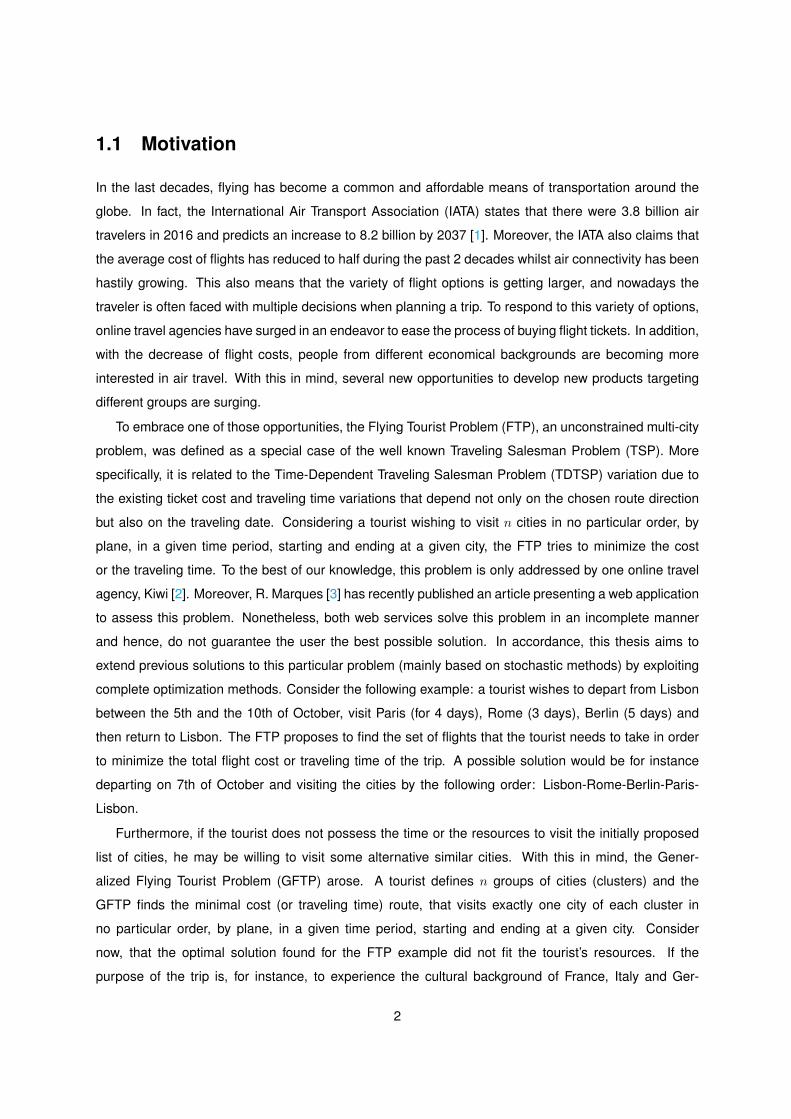
1.1 Motivation

In the last decades, flying has become a common and affordable means of transportation around the

globe. In fact, the International Air Transport Association (IATA) states that there were 3.8 billion air

travelers in 2016 and predicts an increase to 8.2 billion by 2037 [1]. Moreover, the IATA also claims that

the average cost of flights has reduced to half during the past 2 decades whilst air connectivity has been

hastily growing. This also means that the variety of flight options is getting larger, and nowadays the

traveler is often faced with multiple decisions when planning a trip. To respond to this variety of options,

online travel agencies have surged in an endeavor to ease the process of buying flight tickets. In addition,

with the decrease of flight costs, people from different economical backgrounds are becoming more

interested in air travel. With this in mind, several new opportunities to develop new products targeting

different groups are surging.

To embrace one of those opportunities, the Flying Tourist Problem (FTP), an unconstrained multi-city

problem, was defined as a special case of the well known Traveling Salesman Problem (TSP). More

specifically, it is related to the Time-Dependent Traveling Salesman Problem (TDTSP) variation due to

the existing ticket cost and traveling time variations that depend not only on the chosen route direction

but also on the traveling date. Considering a tourist wishing to visit n cities in no particular order, by

plane, in a given time period, starting and ending at a given city, the FTP tries to minimize the cost

or the traveling time. To the best of our knowledge, this problem is only addressed by one online travel

agency, Kiwi [2]. Moreover, R. Marques [3] has recently published an article presenting a web application

to assess this problem. Nonetheless, both web services solve this problem in an incomplete manner

and hence, do not guarantee the user the best possible solution. In accordance, this thesis aims to

extend previous solutions to this particular problem (mainly based on stochastic methods) by exploiting

complete optimization methods. Consider the following example: a tourist wishes to depart from Lisbon

between the 5th and the 10th of October, visit Paris (for 4 days), Rome (3 days), Berlin (5 days) and

then return to Lisbon. The FTP proposes to find the set of flights that the tourist needs to take in order

to minimize the total flight cost or traveling time of the trip. A possible solution would be for instance

departing on 7th of October and visiting the cities by the following order: Lisbon-Rome-Berlin-Paris-

Lisbon.

Furthermore, if the tourist does not possess the time or the resources to visit the initially proposed

list of cities, he may be willing to visit some alternative similar cities. With this in mind, the Gener-

alized Flying Tourist Problem (GFTP) arose. A tourist defines n groups of cities (clusters) and the

GFTP finds the minimal cost (or traveling time) route, that visits exactly one city of each cluster in

no particular order, by plane, in a given time period, starting and ending at a given city. Consider

now, that the optimal solution found for the FTP example did not fit the tourist’s resources. If the

purpose of the trip is, for instance, to experience the cultural background of France, Italy and Ger-

2

many, the tourist might want to consider alternatives to his initial choices. The tourist might then de-

fine the first group of cities as Paris and Marseille, the second group of cities as Rome, Milan and

Venice and the third group of cities as Berlin, Munich and Stuttgart. This results in the following list

(Paris,Marseille),(Rome,Milan,Venice),(Berlin,Munich,Stuttgart). Accordingly, he also defines the days

he wishes to stay at each city (3,2),(3,2,2),(5,5,3). The GFTP proposes to find the set of flights that

the tourist needs to take in order to minimize the total flight cost or traveling time of the trip. An example

of a solution to this problem would be departing on the 8th of October and visiting this set of cities by the

following order: Lisbon-Milan-Berlin-Marseille-Lisbon.

Finally, regarding both the FTP and the GFTP, the tourist may wish to optimize for both the cost

and the traveling time. Therefore, the multi-objective formulations of the aforementioned problems were

derived and are respectively the Multi-objective Flying Tourist Problem (MO-FTP) and Multi-objective

Generalized Flying Tourist Problem (MO-GFTP). Consider that the solutions of the preceding examples

were found in a total flight cost minimization problem. If the traveling time of these solutions is too

large for the tourist, then, by using these multi-objective formulations, he will be able to make a trade-off

between the total flight cost and the total traveling time.

Industry Parallelism: Even though the present section depicts the main motivation behind this thesis,

the developed work has a vast number of applications. For instance, the airline industry faces chal-

lenges similar to the ones this work aims to resolve. Some examples of such problems are the Fleet

Assignment, Aircraft Routing, Crew Pairing and Crew Rostering.

Moreover, the problems addressed by this work can be posed for tourism unrelated issues. Consid-

ering the transportation sector, the FTP can be used to minimize the travel costs of a certain cargo ship.

Furthermore, the freight transportation by air or ship are not as optimized for small routes as ground

transports. Notwithstanding, ground transportation takes longer and cannot deliver overseas. With this

in mind, consider the following example: a logistics company has an air cargo to deliver in various cities

within Europe. Nonetheless, some of this cities are close to each other (e.g inside Iberian Peninsula)

and plane delivery would be too costly. The GFTP shall then be used to plan the air route so that the

cargo is delivered in clusters of cities to then ground transports deliver within each cluster.

1.2 Objectives and Contributions

In this thesis, we propose to optimally solve the unconstrained multi-city problem, FTP, i.e to find the

guaranteed best solution for a certain user request. With this in mind, an Integer Linear Programming

(ILP) formulation for this problem shall be defined. We aim to integrate this formulation in a commercial

solver to find optimal solutions for real life sized, complex multi-city flight requests. Furthermore, this

system shall be compared to existing systems. Next, since the optimal solution might still not suit every

3

end user, we propose to formulate variations of the FTP. Three variations of the FTP should be hypothe-

sized: the Generalized Flying Tourist Problem, the MO-FTP and the MO-GFTP. These formulations aim

to satisfy end users that pretend, for instance, a shorter trip. These formulations should also be solved

using a commercial ILP solver. Finally, the developed work shall be integrated in a web application

prototype.

1.3 Thesis Outline

The presented work is divided into two main studies: the study of complete methods to solve the uncon-

strained multi-city routing problem and its variations, and the evaluation of the results and comparison

to the state-of-the-art. Hence, this document is structured as follows.

Chapter 2 presents a literature review on widely known problems that are related to the FTP, in

particular the Traveling Salesman Problem, and on complete methods to approach these problems.

Chapter 3 introduces a formal definition, as well as ILP formulations for the FTP, GFTP, MO-FTP

and MO-GFTP.

Chapter 4 gives an overview of the development and design choices of the web application that was

used during this work, as well as the modifications that were conducted for its adaptability to the new

models that were proposed.

Chapter 5 outlines the results achieved with this work, comparing the complete method applied here

with the existing work on this problem, as well as the results of the FTP’s variations.

Finally, Chapter 6 describes the main conclusions of this work, and addresses the future work that

could greatly benefit the aforementioned work in a real time web service.

4

2Background

Contents2.1 The Traveling Salesman Problem . . . . . . . . . . . . . . . . . . . . . . . . . . . . . . 62.2 Optimization Techniques . . . . . . . . . . . . . . . . . . . . . . . . . . . . . . . . . . . 16

5

As it was referred in the previous chapter, this thesis addresses Combinatorial Optimization Problems

(COPs), more specifically variations of the Traveling Salesman Problem (TSP). This chapter formally

introduces the TSP in Section 2.1 followed by a description of several approaches to its resolution

presented in Section 2.2. In Subsection 2.2.1, an exact approach is introduced. Finally, Subsection

2.2.2 presents other alternative techniques.

2.1 The Traveling Salesman Problem

As per Dantzig et al. [4], the traveling salesman problem is described as: ”Find the shortest route (tour)

for a salesman starting from a given city, visiting each of a specified group of cities, and then returning

to the origin point of departure. More generally, given an n by n symmetric matrix D = (dIJ), where dIJ

represents the ’distance’ from I to J , arrange the points in a cyclic order in such a way that the sum of

the dIJ between consecutive points is minimal.”

This problem has been studied by three main scientific branches (Operations Research, Applied

Mathematics and Theoretical Computer Science). All these disciplines consider this problem as part of

a broader topic: Combinatorial Optimization.

A Combinatorial Optimization Problem, as explained by Papadimitriou and Steiglitz [5], consists of a

model P = (S,Ω, f) where:

• S is a search space, defined by a finite set of decision variables, each with a domain;

• Ω is a set of constraints amongst the decision variables;

• f : S → R0, is an objective function to be minimized.

Moreover, as stated by complexity theory adopted in Computer Science, these problems are divided

and classified according to their inherent difficulty. Figure (2.1) illustrates how the complexity of these

problems grows. P is the complexity class of problems that are solvable in polynomial time. These

polynomial time algorithms are characterized by a computation time that is bounded by O(p(n)), where

p is a polynomial function and n states the size of the problem. Any problem that is solvable in a

short amount of time is classified as tractable. Hence, most P problems are tractable and vice-versa.

However, this relation is not always true, as tractable means ”efficiently solvable” which is not true for P

problems with large coefficients. On the other hand, NP , or non-deterministic polynomial time, is the

class of problems that given an answer, the proof is verifiable in polynomial time. NP-hard problems are

commonly described as ”at least as hard as the hardest problems in NP ”. The subclass NP-complete,

contained by the NP-hard problems, contains the most difficult problems in NP . If there is an algorithm

that is able to solve one of these problems in polynomial time then, all NP problems are solvable in

polynomial time. Furthermore, such an algorithm would also answer the Millennium Problem ”P vs

NP ”.

6

Lastly, as in the TSP the salesman is required to visit each city exactly once, then the path travelled

is an Hamiltonian path1. Moreover, as the salesman is to return to the origin city, this is an Hamiltonian

cycle2. Determining the existence of an Hamiltonian cycle in a graph is a NP-complete problem, which

implies that the TSP is also NP-complete [6].

NP

P

NP-Complete

NP-Hard

Figure 2.1: P vs NP if P 6= NP .

Integer Linear Programming

Integer Linear Programming (ILP) is a mathematical program with integer variables, where both the

objective function and the constraints are linear. If not all decision variables are discrete, then the

program is known as a Mixed Integer Linear Program (MILP). In the case where all variables are binary,

the problem is called a 0-1 ILP [5, 7]. This is defined in the canonical form as:

minn∑

j=1

cjxj

s.t.n∑

j=1

aijxj ≤ bi 1 ≤ i ≤ m,

xj ∈ N0 1 ≤ j ≤ n.

(2.1)

1In graph theory, an Hamiltonian path is a graph that visits every vertex exactly once.2In graph theory, a cycle is a directed or undirected path that only repeats the first (and last) vertex.

7

where xj are the decision variables, cj and bi are the elements of coefficient vectors and aij are the

entries of the coefficient matrix. For instance, considering the following problem:

min y

s.t. y ≥ 3x− 3,

y ≤ x + 2,

y ≥ −3x + 3

x, y ∈ N0.

(2.2)

The linear programming solution is represented in Figure 2.2. The red, blue and violet lines represent

the constraints, respectively. These three lines together also define the polyhedron of the Linear Program

relaxation3. The black dashed line represents the convex hull that contains all the feasible integer points,

shown in black. Considering the minimization problem, the optimization problem hence finds the solution

(1, 0). This is also the solution of the Linear Program relaxation. On the other hand, if this was instead

a maximization problem, the solution would be (2, 4) which is different than its relaxation, (2.5, 4.5).

Figure 2.2: Graphical representation of Equation (2.2).

TSP Problem Statement

The TSP can be defined as a graph G = (N,A),4 with N being the set of nodes of size n = |N | and

A the set of arcs connecting the nodes of size n2. The arcs are hence represented as (i, j) ∈ A, i 6= j

3Linear Program relaxation is the Linear Program without integrality constraints. This concept is explained in detail further inthis work.

4In some literature this is defined as G = (V,E) where V is the set of vertices and E is the set of edges instead.

8

and have an attached weight matrix of cij . Problems in which the triangle inequality (cik + ckj ≥ cij for

all i, j, k ∈ N ) is satisfied are called Euclidean problems [8]. In the literature, this matrix has several

designations as it can describe distance, cost, time or even a weighted variable. A is often assumed

to be complete, this means that every distinct node is connected by one and one only arc, and the

missing arcs are replaced with large weights thus making a connected and weighted graph. Moreover,

in the standard TSP, G is also defined as undirected, resulting in the well known Symmetric Traveling

Salesman Problem (STSP), where cij = cji,∀i, j ∈ N . On the other hand, if G is directed, the problem is

more general and is named Asymmetric Traveling Salesman Problem (ATSP). These problems can be

transformed in one another with ease. If one duplicates the arcs of a STSP and considers the undirected

graph as a directed one, then the STSP is converted into an ATSP. On the other hand, if instead, the

nodes are duplicated, it is possible to transform an ATSP into an equivalent STSP. This transformation

can be seen in Figure 2.3. For deeper insight on the transformation between the two, the reader is

referred to [9, 10].

Figure 2.3: Transformation of an ATSP instance (left side) into a STSP instance(right side) [10]. M is asufficiently large number and represents the weight of the associated arcs.

The TSP has innumerous variations. A brief introduction of the most common variations, as well as

a more thorough description for the much relevant variations that underpin the work under development,

based on the formulations presented in [11], is presented next.

2.1.1 Dantzig-Fulkerson-Johnson ATSP Model

Integer linear programming (ILP) addresses an optimization problem focused on the minimization of a

linear objective function amidst the integer points of a polytope P [12]. In the case of a three dimensional

problem the polytope is a polyhedron.

The particular case of the ATSP can be formulated as an ILP model. Dantzig et al. [4]:

9

minn∑

i=1

n∑j=1

cijxij (2.3)

s.t.n∑

i=1

xij = 1 j = 1, . . . , n, (2.4)

n∑j=1

xij = 1 i = 1, . . . , n, (2.5)

∑i∈S

∑j∈S

xij ≤ |S| − 1 S ⊂ V : S 6= ∅, (2.6)

xij ∈ 0, 1 i, j = 1, . . . , n. (2.7)

Every arc (i, j) ∈ A is associated with a binary variable xij and a corresponding weight cij . The

number of variables is n2 and the decision variable space has a size of 2n2

. An arc is part of the optimal

tour, and hence part of the solution, when the associated decision variable is assigned the value 1.

Constraints (2.4) and (2.5) state that each vertex has exactly one arc entering and one arc leaving,

enforcing the tour to be an Hamiltonian path. Constraints (2.6) are Subtour Elimination Constraints

(SECs) and impose that subtours, i.e partial circuits, are excluded. The latter group of constraints can

be equivalently rewritten as Connectivity constraints:

∑i∈S

∑j∈V \S

xij ≥ 1 S ⊂ V : S 6= ∅, (2.8)

Lastly, constraints (2.7) impose that decision variables are either equal to 0 or 1. The previous ILP

model has an exponential number of SECs and a lower bound on the optimal solution may be obtained

through LP relaxation by removing the integrality constraint of each variable.

Polynomial Formulations

Having an exponential number of SECs would greatly increase the computational time, thus a few poly-

nomial formulations for the ATSP are considered.

Remark 1. Notice that in this section, by polynomial formulations we mean, formulations in which

the number of subtour elimination constraintsa grows with a polynomial factor with the size of the

problem.aSubtour elimination constraints forbid the existence of solutions consisting of several subtours.

Roberti, Toth. [13] present a review of polynomial formulations and report that the best formulations

to be used are Miller, Tucker and Zemlin [14], Gavish and Graves [15] and Desrochers and Laporte [16]

(MTZ, GG and DL, respectively). All of these formulations consist on DFJ model replacing (2.6) with

another group of constraints.

10

MTZ achieves this by creating a group of integer decision variables ui. These variables represent

the order of vertex i in the optimal tour. The constraints are defined as follows:

ui − uj + (n− 1)xij ≤ n− 2, i, j = 2, . . . , n. (2.9)

On the other hand, GG creates n(n− 1) integer variables gij that represent the number of arcs from

node 1 to arc (i, j) in the optimal tour as well as the following constraints:

n∑j=1

gij −n∑

j=2

gji = 1, i = 2, . . . , n, (2.10)

0 ≤ gij ≤ (n− 1)xij , i = 2, . . . , n j = 1, . . . , n. (2.11)

Finally DL is an enhanced MTZ formulation and hence utilizes the same decision variables ui. The

constraints are:

ui − uj + (n− 1)xij + (n− 3)xji ≤ n− 2, i, j = 2, . . . , n, (2.12)

− uip(n− 3)xi1 +

n∑j=2

xji ≤ −1, i = 2, . . . , n, (2.13)

ui + (n− 3)x1i +

n∑j=2

xij ≤ n− 1, i = 2, . . . , n. (2.14)

Both GG and DL present formulations having stronger LP relaxation than that of MTZ. A strong, or

tight, LP relaxation means that the feasible set of the relaxation is close to the convex hull of integer

feasible solutions and thus, the optimal solution of both GG and DL are more likely to be closer to the

integer optimum than the optimal solution of the MTZ.

2.1.2 The Time Dependent Traveling Salesman Problem

The Time-Dependent Traveling Salesman Problem (TDTSP) is a generalization of the TSP, where the

cost of the arcs connecting the nodes depends on the time at which the salesman traverses the arc. This

model has several real-world applications as the one-machine sequencing problem. The TDTSP can be

defined as a oriented graph G = (N,A) with the condition that for each arc (i, j) ∈ A the travel cost at

period k = 1, 2, . . . , n is defined as ckij . This problem was first addressed by Fox in 1973 [17] and later

revisited in 1980 with the help of Gavish and Graves [18]. In 1978, Picard and Queyranne [19] proposed

what is now the basis of this problem using O(n3) variables and O(n2) constraints as the following:

In this formulation, xkij are the decision variables. These are assigned the value 1 if the arc (i, j)

on time instance k is taken, and 0 otherwise. Constraints 2.16 guarantee that the cycle leaves each

city once and once only in the comprised time-window. Constraints 2.17 and 2.19 ensure that the cycle

starts and finishes on node 1 on days 1 and n, respectively. Constraints 2.18 assure that the inflow on

11

Figure 2.4: Example of a multipartite TDTSP network with n = 4 cities [21].

day k at each node is the same as the outflow on day k + 1, which eliminates subtours5 and controls the

time spent at each node. Lastly, Constraints 2.20 are integrality constraints and secure that the decision

variables are binary. Defining now that a state is a pair node-time (i, k), then the decision variables xki,j

represent the transition from state (i, k) to state (j, k + 1). Considering a multipartite network, where the

state (1, 1) is the source and (1, n + 1) is the sink, then a 4 city TDTSP can be represented as in Figure

2.4.

minn∑

i=1

n∑j=1

n∑k=1

ckijxkij (2.15)

s.t.n∑

i=1

n∑k=1

xkij = 1, j = 1, . . . , n (2.16)

∑(1,j)∈A

x11j = 1, (2.17)

∑(i,j)∈A

xkij −

∑(j,i)∈A

xk+1ji = 0, t = 2, . . . , n− 1, j = 1, . . . , n (2.18)

∑(i,1)∈A

xni1 = 1, (2.19)

xkij ∈ 0, 1 i, j, k = 1, . . . , n. (2.20)

The objective of this problem is the same as the TSP: find the minimum cost Hamiltonian cycle over

the graph G = (N,A).

2.1.3 Traveling Salesman Problem With Time Windows

The Traveling Salesman Problem with Time Windows (TSP-TW) is defined as a generalization of the

TSP with changeover times over nodes, represented as setup times tij , as well as the processing time

pj ≥ 0, release date rj ≥ 0 and deadline dj ≥ rj for every node j ∈ N . The time window referred for

node j is thus [rj , dj ]. The objective of this variation is to find the minimum cost Hamiltonian path (cycle

5Subtours are solutions consisting of several disconnected tours [20].

12

if faced with a closed-tour variation) visiting a node sequence such that for every node, the processing

time lies in the time-window. If the time-window is [0,+∞] then it is relaxed. On the other hand, if this

interval is characterized by rj > 0 and dj < +∞ then the time-window is active.

The Asymmetric TSP-TW is very important when dealing with scheduling and routing problems [22].

Considering an Asymmetric TSP-TW instance defined on a complete digraph G = (V,A), the convex hull

of the eigenvectors of all the feasible paths contained in such graph can be represented as a polytope.

Finding the dimension of such polytope is a NP-complete problem even when all time windows with the

exception of one are relaxed [22].

2.1.4 Generalized Traveling Salesman Problem

The Generalized Traveling Salesman Problem (GTSP), or set TSP, is an extension of the TSP. This

problem consists on determining the shortest or minimum cost route that passes through each cluster

of nodes at least once and never repeats a node. It assumes that N is a set of clusters containing

every node and the clusters are formed by at least one node. Let G = (N,A) be a m-node weighted

undirected graph where each arc contained in A is associated with a non-negative cost cij . Furthermore,

N is partitioned in n disjoint subsets or clusters Sl, l = 1, . . . , n.

In the following ILP model, the integer variables xij take the value 1 if the arc between nodes i and

j is used and the value 0 otherwise. Variables yi and y′

i refer to the outflow and inflow of each node i,

respectively. For each node i they are assigned the same value, 1 when node i is visited and 0 otherwise.

min∑i∈N

∑j∈N\i

cijxij (2.21)

s.t.∑

j∈N\i

xji = y′

i i ∈ N, (2.22)

∑j∈N\i

xij = yi, i ∈ N, (2.23)

∑i∈Sl

yi =∑i∈Sl

y′

i ≥ 1, l = 1, . . . , n, (2.24)

yi = y′

i, i ∈ N, (2.25)∑i∈T

∑j∈T\j

xij ≤ |T | − 1, T ⊆ N, T ∩ Sl = ∅ for at least but not all l, (2.26)

xij , yi, y′

i ∈ 0, 1 i, j ∈ N, i 6= j (2.27)

Constraints 2.22 and 2.23 state the inflow and outflow of each node i. Constraints 2.24 force each

cluster to be visited at least once. Constraints 2.26 are subtour elimination constraints. Finally, con-

straints 2.27 are integrality constraints. The reader is referenced to [8] for further insight and more detail

13

8

2

3

1

3

4

6

5

5

8

4

10

Cluster 1

Cluster 2

Cluster 3

5

Figure 2.5: Generalized Traveling Salesman Problem.

on the previous formulation and how to improve it. In the literature, other authors also formulate the

GTSP more strictly, stating that each cluster should be visited once and once only by imposing that the

tour includes exactly one node from each node set [23, 24]. This difference only changes constraints

2.24, which would become:∑

i∈Slyi =

∑i∈Sl

y′

i = 1, l = 1, . . . , n. A diagram of the latter formulation

is shown in Figure 2.5. This diagram represents a GTSP with 3 clusters. The first and third clusters

contain 2 cities and the second contains 1 city. The black lines represent all the possible arcs, whilst the

red lines represent the shortest Hamiltonian cycle of this problem.

2.1.5 Multi-Objective Traveling Salesman Problem

The Multi-objective Traveling Salesman Problem (MO-TSP) is another generalization of the TSP. How-

ever, instead of solely minimizing the distance/cost of the tour, it tries to respond to a set of different

objective functions. This problem is often associated with a wider set, the multi-objective COPs [25].

For the formal definition of this problem, several definitions must be understood. Firstly, a Multi-

objective Problem (MOP) is defined in [26] as:

14

minn∑

j=1

c1j xj

. . .

n∑j=1

ckj xj

s.t.n∑

j=1

aijxj ≤ bi 1 ≤ i ≤ m,

xj ∈ N0 1 ≤ j ≤ n.

(2.28)

where each arc has k associated weights ckj .

For easiness of explaining the rest of the definitions on this section, F (~x) is defined as the k di-

mensional objective set that comprises the objective functions∑n

j=1 c1jxj , . . . ,

∑nj=1 c

kjxj , where ~x =

(x1, . . . , xn) is a n-dimensional decision variable vector from some universe Ω.

Moreover, the terminology related to Pareto concepts is also of the utmost importance in MOPs.

Pareto Dominance is defined as follows: A vector ~u = (u1, . . . , uk) is said to dominate ~v = (v1, . . . , vk),

represented as ~u ~v, if and only if ~u is partially less than ~v, i.e ∀i ∈ 1, . . . , k, ui ≤ vi ∧∃i ∈ 1, . . . , k :

ui < vi. On the other hand, Pareto Optimality is stated as: A solution x ∈ Ω is said to be Pareto optimal

with respect to Ω if and only if there is no x′ ∈ Ω for which ~v = F (x′) = (f1(x′), . . . , fk(x′))) dominates

~u = F (x) = (f1(x), . . . , fk(x)). Pareto Optimal Set is defined as follows: For a given MOP, the Pareto

optimal set (P ∗), is defined as:

P ∗ := x ∈ Ω | ¬∃ x′ ∈ Ω : F (x′) F (x)

Lastly, for a given MOP F (x) and Pareto optimal set P ∗ the Pareto front PF ∗ is defined as:

PF ∗ := ~u = F (~x) = (f1(x), . . . , fk(x)) | x ∈ P ∗

The previous concepts refer to the Pareto global optimum set. In the case of the MO-TSP, finding

this set is NP-hard. With this in mind, it is important to also consider the Pareto local optimum sets

instead, as this can have improvements in the computational time. The definitions are very similar to the

ones above with the inclusion of a neighbourhood in the evaluation of the Pareto optimum solutions. For

more insight refer to [27].

Lastly, understanding all of the above concepts, the MO-TSP definition is as follows: Let G = (N,A, c)

be a complete and weighted graph where N is the set of nodes, A is the set of arcs connecting the

nodes and c the cost/distance associated with each arc. The multi-objective TSP finds one or more

Pareto optimal Hamiltonian tours, or cycle in a closed problem, of the graph visiting each node exactly

once.

15

2.2 Optimization Techniques

This section introduces two different approaches to solve COPs. In Subsection 2.2.1, Linear Program-

ming (LP) is presented, as well as a specific model where this approach is applied to the ATSP. Af-

terwards, we present a small overview of other methods that have advantages relative to LP in some

situations.

2.2.1 Linear Programming

Linear Programming (LP) is a specific technique of mathematical programming for the optimization of a

linear objective function subject to linear equality and inequality constraints. When a feasible problem

is considered, this method achieves at least one optimal solution. Infeasibility means that the method

proved that there is no solution that respects all the constraints. A LP formulation can also be interpreted

as a geometrical problem where the feasible region is a convex polytope with at least one of its vertices

being an optimal solution.

2.2.1.A Branch and Cut Algorithms

Branch and Cut (B&C) methods are exact algorithms6 used in integer programming problems. These

methods solve a series of linear programming relaxations of the problem, apply cutting plane methods7

to further improve the relaxation of the problem, followed by the application of Branch and Bound (B&B)

algorithms to solve the problem in a divide-and-conquer8 approach. These methods are also usually

aided by preprocessing, primal heuristics, as well as lifting/strengthen constraint techniques [29]. Even

though some problems might be too large to be handled by these methods, the nature of such algorithms

make it possible to exploit coarse grain parallel computing, which divides a program in various large tasks

to be computed separately by various processors.

In an optimization problem, relaxation is responsible for finding bounds, lower bounds in minimization

and upper bounds in maximization, on the optimal value. With this in mind, relaxation bounds are

important to calculate the relative gap, how close to the optimum is the suboptimal solution, and to

accelerate the search. By defining bounds, if the bounds of a certain node are worse than the incumbent

solution9., then that node will no longer be branched.

Cutting plane methods are usually very useful when combined with a B&B algorithm. However, very

ineffective when used standalone. These methods are based on sequential LP relaxations to better

approximate the problem. Developed by R.E.Gomory [30], at first these algorithms seemed to be weak.

Nonetheless, with the observed progresses in polyhedral theory, these algorithms were revamped and

6An exact algorithm solves a problem to optimality (if faced with a NP-hard problem in exponential time).7Cutting planes method iteratively applies linear inequalities, called cuts, refining the feasible set. For more insight [28].8Divide-and-Conquer is a generic framework (algorithm paradigm) that using recursion breaks problems into sub-problems.9Incumbent solution is the best integral feasible solution of the integer program

16

they are today a cutting edge method in some COPs. The basic structure of such techniques is as

follows:

Algorithm 1 Cutting Planes Method1: while True do2: Solve the LP Relaxation;3: if feasible solution is found then4: Optimality achieved;5: break While.6: else7: Apply more cutting planes to separate the solution, given by the relaxation, from the feasible

points convex hull.

Usually, the first relaxation is solved using the primal simplex algorithm. The following are then more

commonly solved by applying dual10 simplex. This happens as the applied cutting planes often make

primal simplex infeasible. Cutting plane methods are also of such importance as they return provably

optimal solutions or, when an instance cannot be solved to optimality, bounds on the optimal value [32].

B&B is the most used approach when it comes to integer programs. A more thorough description

of this algorithm is as follows: by iteratively partitioning the set in subsets, or branches, and creating

bounds for each branch, its effectiveness comes from the fact that, in a minimization problem, if a lower

bound for the objective value of a certain subproblem is larger than the objective value of an integer

feasible solution, then the optimal solution does not lie in the respective subproblem. Another concept to

be understood in B&B algorithms is that a relaxation of an optimization problem is also an optimization

problem and solving a relaxation of the problem provides a lower bound for the ILP problem. This

implementation can be compared to a tree search, where the integer problem is the root. A general

assertion of a B&B algorithm is as follows [33]:

1. (Initialization): Form a set of subproblems as the original integer program and initialize the upper

bound of these subproblems to∞.

2. (Termination): If the set of subproblems is empty then the saved solution is optimal. If such solution

does not exist, then the problem is infeasible.

3. (Problem selection and relaxation): Select and delete a subproblem from the set. Solve a relax-

ation of this subproblem and get the optimal objective value of such relaxation.

4. (Fathoming and Pruning): This step deals with the nodes that are no longer necessary to be

explored. When all the nodes are fathomed, the search ends.

10In simple terms, the dual of a LP is achieved by transforming the variables of the primal into constraints, the constraints of theprimal into variables and inversing the objective. If the duality is strong then the optimal value exists for both and is the same. Ifthe duality is weak then the objective value of the dual at any feasible solution is a bound of the primal [31].

17

(a) If the optimal objective value of the relaxation is greater or equal to the incumbent objective

value, return to step 2.

(b) else, if the optimal objective value of the relaxation is less than the incumbent objective value

and if the optimal solution of the relaxation is integral, then the optimal objective value of the

relaxation is the new incumbent objective value. In addition, delete all the subproblems with

lower bounds greater than the new incumbent objective value. Return to step 2.

5. (Partitioning): Considering a partition of the constraint set of a subproblem, add new subproblems,

with the feasible region restricted to the new partition of the contraint set, to the whole set of

subproblems and establish the lower bounds as the actual incumbent objective value. Return to

step 2.

It is important to keep in mind that several partitioning strategies exist. These typically use linear

constraints and form two new nodes at each division. During this process, branching variables are

selected to create more nodes. Several methods of branching and variable selection exist and their

usage mostly depend on the type of integer program. The strategy that generally comes after is the

node selection. This affects the chance of node fathoming hence the number of problems to be solved

before optimality. Nonetheless, B&B has its flaws. For instance, in very large problems, integer feasible

solutions may not be found at first, which leads to an accumulation of several active nodes, thus resulting

in memory explosion. To counteract this possibility, cutting planes are often added to the root node to

strengthen the LP formulation. Several preprocessing techniques, used either before or during B&B, can

also greatly improve these methods. Some examples of such techniques are the removal of empty or

dependent rows/columns, aggregation, coefficient reduction, logical implications and probing. We refer

the reader to [34] for more details on these techniques. Moreover, heuristic approaches can also be

used to obtain solutions in a fast manner. In B&B, heuristics are used to produce a good upper bound

for reduced cost fixing at the root, hence reducing the size of the LP. With the purpose of achieving a

good result in a small ammount of time, heuristics are underpinned by the following five crucial methods

[33]:

• Greediness: Choose the variable based on the best local outcome.

• Local Search: Search in a neighbourhood of a feasible solution for a better objective value. Exam-

ples of such methods are for instance Simulated annealing [35] and Hill climbing.

• Randomized enumeration: Based on random factors. Genetic algorithms [36] are good examples

of this foundation.

• Primal heuristics: LP-based procedure that solve a modified problem where a good solution is

found in a point that fails to satisfy integrality.

18

• Primal-Dual interplay: Usage of solutions from the dual problem in the primal problem and vice-

versa.

Heuristics make use of at least one of the above methods. Even when using all these methods, some

large scale problems may present some difficulties. In such contexts, using interior point algorithms,

as the LP solver, can have promising results. Interior point methods reach the optimal solution by

transversing the interior of the feasible region. Since Karmakar breakthrough in 1984, these methods

can be more efficient than the simplex algorithms in many settings [37, 38].

2.2.1.B LP Solvers

In this subsection, an overview of two different mathematical optimization problem solvers is presented

as well as a comparison between both. This was conducted in order to achieve the best possible

results for the rest of this work. Only two commercial software tools, CPLEX and Gurobi, are presented

as these are typically the ones referenced by the state-of-the-art literature. The benchmarks in [39]

are referenced in several sources. However, these benchmarks were removed due to requests of the

solver’s developers. On the other hand, it is important to notice that the problems tackled through this

work can be solved with a vast number of other solvers like GLPK, LP Solve, SCIP or even the comercial

solver Xpress.

CPLEX

The ILOG IBM Optimization Studio is a high-performance mathematical programming solver for linear

programming, mixed-integer programming and quadratic programming [40]. Presented with an integer

linear program, this solver resorts to 3 different algorithms:

• The simplex algorithm is an iterative method that starts with an initial feasible solution (a vertex of

the polytope) and moves progressively over the neighbourhood until optimality is achieved.

• The dual simplex algorithm starts with any optimal solution and iterates until feasibility is reached.

• The barrier methods, also known as interior point methods, start somewhere inside the feasibility

region and using a predictor-corrector algorithm follow a central path through the interior until an

optimal solution is found.

In addition, before using any of these algorithms to solve the model, CPLEX runs a presolve proce-

dure that attempts to reduce the size of the problem by removing redundant constraints.

This optimization software, created by Robert E. Bixby, is currently developed by IBM and it is im-

plemented in C languange. However, as of today, different interfaces to C++, C#, Java and Python

languages as well as Matlab also exist. Moreover, this optimizer is also accesible through modeling

systems [41].

19

Gurobi

Gurobi is another modern solver for mathematical optimization problems. Robert E. Bixby is, again, one

of the creators of this software implemented in C. This optimizer also supports interfaces for C++, C#,

Java, Python, .NET, Matlab and R. Furthermore, it can also solve non-linear problems and has a cloud-

server system, where problems can be deployed. As of February 2019, the developers of this solver

claim better results than any other mathematical problem solving software in [42].

Comparison of both

According to [41], for large scale problems, free solvers fall behind the comercial ones like CPLEX and

Gurobi. When comparing these two, the results are fairly similar and problem dependent. This means

that depending on the problem, the performance of one may be better than the other and vice-versa.

Nonetheless, authors commonly adress Gurobi as the fastest solver whilst CPLEX as the most robust.

For the previously mentioned reasons, these were the only two solvers considered throughout this work.

2.2.2 Other Techniques

Even though the approaches presented in the previous section allow to achieve an exact optimal solu-

tion, this can be very demanding. In some cases, complete methods cannot find a feasible solution in

a reasonable amount of time. With this in mind, several incomplete methods11 that find solutions in a

faster manner are discussed in this section.

2.2.2.A Heuristic Algorithms

An incomplete method of solving NP-hard problems is through heuristics. An heuristic is any technique

that in a small amount of time is able to find a solution for a given problem. Usually these are divided in

construction or improvement heuristics. For more insight on heuristics, the reader is referenced to [43].

Held-Karp Lower Bound

As previously explained, complete algorithms allow to prove optimality. Even when that does not happen,

an absolute or relative gap towards the best possible solution is easily computed. However, when using

heuristics this is not necessarily the case. As a result, the evaluation of the quality of a certain heuristic

is not straightforward. With this purpose, a lower bound, called Held-Karp (HK) lower bound, is often

computed. This lower bound is achieved either by computing the solution of a linear programming

relaxation of the ILP model, computed in polynomial time, or through an iterative algorithm that computes

minimum spanning trees [44].

11Incomplete methods cannot guarantee the quality of the solution found.

20

Tour Construction

Tour construction algorithms use heuristics to construct a solution. Next, three different common tour

construction algorithms are presented.

The Nearest Neighbour (NN) heuristic proceeds in three different steps. First, a random node

is selected for the beginning of the path. Step 2 consists on finding the nearest node relative to the

previously selected one and adding it to the path. Finally, step 2 is repeated until all nodes are contained

in the tour and the last node is connected to the first [45]. This algorithm requires n2 computations, where

n denotes the number of nodes, and generally finds a solution within 25% of the HK lower bound [43].

The Greedy algorithm is very similar to the NN and some authors even consider it the same. Steps

2 and 3 are the same as of the NN. Nonetheless, instead of choosing the first node randomly in step

1, the arcs are all sorted according to their weight and the smallest one is chosen. With this change, a

better solution can be found (often within 20% of the HK lower bound) with the downside of increasing

the computational complexity to O(n2log2(n)) [43].

Insertion heuristics can also be very useful, sometimes presenting improvements relative to the

ones presented previously. These heuristics begin with the creation of a subtour with the inclusion of the

rest of the nodes by some heuristic. For instance, the Nearest Insertion starts by finding the minimum

cost arc and forms a subtour. After that, it searches for the node that forms the minimum weight arc

with any of the nodes already present on the subtour and inserts it. This final process is repeated until

the Hamiltonian cycle is formed [45]. These heuristics have a computational complexity on the order of

O(n2) and often present a solution with a relative gap to HK of less than 20%.

Tour Improvement

After constructing a tour, one may wish to improve this solution. Keeping this objective in mind, perhaps

the most used heuristics with this purpose are the branch exchange heuristics. The 2-opt, k-opt and,

later introduced by Lin and Kernighan, the Lin-Kernighan algorithm, are discussed next [46].

The 2-opt and k-opt algorithms work by removing 2 and k branches, respectively, from the tour and

reconnecting the paths. This process is only done if the new tours are shorter and is repeated until 2-opt

or k-opt improvements are no longer possible, resulting in 2-optimal and k-optimal tours respectively.

Notice that a k-optimal tour is also (k-1)-optimal and hence 2-optimal. The 2-opt heuristic generally

results in a solution within 5% of the HK lower bound [45].

The Lin-Kernighan algorithm [46] finds a feasible solution for the symmetric TSP with a time com-

plexity of approximately O(n2.2). It is a variation of the k-opt heuristic that at each step decides how

many paths it should switch to find the minimum weight tour.

21

2.2.2.B Meta-Heuristic Algorithms

Meta-heuristics are algorithms that are designed to be applied to any COP. These are generally based

on concepts from biological evolution, physics or even statistical mechanics and include for example,

Genetic Algorithms, Simulated Annealing, Tabu-Search, Ant Colony Optimization or even Neural New-

torks [47]. This subsection introduces some of these algorithms.

Ant Colony Optimization is based on the behaviour of real ants. When traveling from the nest

to a food source, ants seem to all take the same path and curiously, the shortest one as well. This

does not happen at first but when ants walk they leave a pheromone trail. Ants are also probabilistically

more prone to take a trail that has more concentration of that pheromone [48]. Considering various

paths, ants pass more often on the same spot in a shorter one. Hence, in this path there will be more

concentration of that pheromone, leading to more ants choosing this trail which positively feedbacks

the other ants, eventually leading this path to be the only one taken. Simulating a TSP with artificial

ants might then have surprising results if one identifies an appropriate representation of the problem. A

good heuristic to determine the distance/weight between two cities and a good probabilistic interaction

ant/pheromone model should be used [49]. ACOs are hybrid Stochastic Local Search (SLS) approaches

with both probabilistic solution construction and normal local search techniques [10]. A very effective

ACO algorithm for the TSP is the MAX-MIN Ant System [50].

Simulated Annealing simulates the physical process of heating a metal until the melting point and

then reducing the temperature in a controlled way. This results in a particle arrangement that minimizes

the energy state (ground state of the solid). An analogy to this physical process was used to develop

this metaheuristic. In this analogy, the total weight of the solution corresponds to the energy state and

the particle rearrangement to the solution space [35]. This metaheuristic can then be compared to a

local search heuristic with the tweak that now up-hill moves are possible (in the analogy this would be

the heating process).

Genetic Algorithms are part of the broader class of Evolutionary Algorithms and are inspired by the

natural selection process. These algorithms are based on a five step process. During the initialization,

a population is stochastically created. Then, based on a fitness function, some of the population is

selected to breed another generation. This new generation is subject to genetic operators such as

crossover and mutation. During this process, other heuristics may also be applied. Finally, this steps

are repeated until a termination condition has been satisfied.

22

3Problem Formulation and

Optimization Models

Contents3.1 Flying Tourist Problem . . . . . . . . . . . . . . . . . . . . . . . . . . . . . . . . . . . . 243.2 Generalized Flying Tourist Problem . . . . . . . . . . . . . . . . . . . . . . . . . . . . . 273.3 Multi-objective Flying Tourist Problem . . . . . . . . . . . . . . . . . . . . . . . . . . . 323.4 Multi-Objective Generalized Flying Tourist Problem . . . . . . . . . . . . . . . . . . . 343.5 Final Considerations . . . . . . . . . . . . . . . . . . . . . . . . . . . . . . . . . . . . . 343.6 Summary . . . . . . . . . . . . . . . . . . . . . . . . . . . . . . . . . . . . . . . . . . . . 38

23

In this Chapter, four different ILP models that formalize the Flying Tourist Problem (FTP) and its

considered variations are presented. In Section 3.1, the model presented by R. Marques [3, 51] is

revisited and a different method to solve it is proposed. This model is then modified to answer three

different problems. In Section 3.2, the FTP is modified considering a generalization of the problem,

the Generalized Flying Tourist Problem (GFTP). In Section 3.3, the FTP is adapted based on a multi-

objective optimization, leading to the Multi-objective Flying Tourist Problem (MO-FTP). In Section 3.4 a

final model considering both adaptations, the Multi-objective Generalized Flying Tourist Problem (MO-

GFTP), is presented. Lastly, in Section 3.5, these problems are compared to the original TSP and both

a graph and a dimensional overview of these models are conducted.

3.1 Flying Tourist Problem

The FTP formulates the problem of a tourist that desires to visit several cities by plane in a specified

time-window. The main objective is to minimize the cost or traveling time of the tourist. The solution is

then a set of flights that the tourist should buy in order to minimize one of these objectives. This set of

flights is a Hamiltonian Cycle.

This problem is very close to the TDTSP, as the tourist is to specify the stop-time at each city, and

can be illustrated in a multipartite graph, as shown in Figure 3.1. This is a simple instance, where the

departure and arrival cities are the same, respectively V0 = Vn+1 = VX and it considers 3 intermediate

nodes (VA, VB , VC), each with a fixed stop time, respectively (1,2,3) time units. The starting date window

T0 is singular with t = 0. Moreover, a possible solution to this instance, represented in the figure with

the path corresponding to the set of arrows in red, is given by the set of arcs (A0X,B , A

2B,A, A

3A,C , A

6C,X).

VX0 VB1

VC1

VA1

VB2

VC2

VA2

VB3

VC3

VA3

VB4

VC4

VA4

VB5

VC5

VA5

VB6

VC6

VA6

VX7

Text

nodes

time

Figure 3.1: Multipartite graph of the Flying Tourist Problem [3].

24

Problem statement

Assuming that the user wants to visit a set V of n cities connected by the set of arcs A, the objective of

this model is to minimize the weight function cijk, the weight of the arc connecting nodes i and j on time

instance k, of a tour that starts on origin city 0, visits exactly once all n cities and finishes at arrival city

n + 1. The weight function is defined by the user itself and it can be the travel cost, the traveling time or

a compromise between the two. The user is also the provider of the stop time si at each intermediate

city and the time horizon during which the travel may start T0 = [T0m, T0M ]. Even though (in this work)

the stop time will always be considered as an integer, it may be a range of values instead. With T0 and

si, it is then possible to define a time window during which each city may be visited, denoted by TW .

The set S containing all valid solutions is hereinafter defined and the purpose of this model is to find the

global minimum, by considering the objective function of this set.

The present formulation also took in consideration the work developed by Li et al. [52]. They proposed

a problem that aims to find itineraries with the lowest cost for travelers visiting multiple cities under the

constraints of time horizon and stop time at each city. With this in mind, the travel itinerary problem was

raised and it is fairly similar to what we propose in this subsection.

The notation used in our model is as follows:

• V is the set of city nodes,

• i is the index of the departure city of a certain flight,

• j is the index of the arrival city of a certain flight,

• k is the index of the transport alternative used,

• n is the number of intermediate cities,

• Iij is the number of transport alternatives from city i to city j,

• cijk is the cost value of the flight from city i to city j, using the transport alternative k,

• dijk is the departure date and time from city i to city j, using the transport alternative k,

• ajik is the arrival date and time at city i from city j using the transport alternative k,

• si is the stop time at city i,

• Tstart or T0m is the minimum start date,

• T0M is the maximum start date,

• Tfm is the minimum return date,

25

• Tend or TfM is the maximum return date,

• xijk is a binary decision variable that carries the value 1 if the flight k from city i to city j is taken.

• ui is an integer decision variable that carries the non-negative value associated to the position of

city i in the tour.

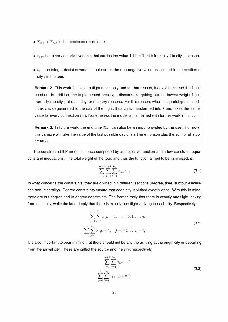
Remark 2. This work focuses on flight travel only and for that reason, index k is instead the flight

number. In addition, the implemented prototype discards everything but the lowest weight flight

from city i to city j at each day for memory reasons. For this reason, when this prototype is used,

index k is degenerated to the day of the flight, thus Iij is transformed into I and takes the same

value for every connection (ij). Nonetheless the model is maintained with further work in mind.

Remark 3. In future work, the end time Tend can also be an input provided by the user. For now,

this variable will take the value of the last possible day of start time horizon plus the sum of all stop

times si.

The constructed ILP model is hence composed by an objective function and a few constraint equa-

tions and inequations. The total weight of the tour, and thus the function aimed to be minimized, is:

n+1∑i=0

n+1∑j=0

Iij∑k=1

cijkxijk (3.1)

In what concerns the constraints, they are divided in 4 different sections (degree, time, subtour elimina-

tion and integrality). Degree constraints ensure that each city is visited exactly once. With this in mind,

there are out-degree and in-degree constraints. The former imply that there is exactly one flight leaving

from each city, while the latter imply that there is exactly one flight arriving to each city. Respectively:

n+1∑j=1

Iij∑k=1

xijk = 1, i = 0, 1, . . . , n,

n∑i=0

Iij∑k=1

xijk = 1, j = 1, 2 . . . , n + 1,

(3.2)

It is also important to bear in mind that there should not be any trip arriving at the origin city or departing

from the arrival city. These are called the source and the sink respectively.

n+1∑i=1

Iij∑k=1

xi0k = 0,

n∑j=0

Iij∑k=1

x(n+1)jk = 0,

(3.3)

26

Remark 4. If the origin city and the destination city are the same, then we are facing a cycle and

the degree constraints are still consistent. In this case, the origin/destination city is both the source

and the sink of the problem.

Time constraints assure that the start time Tstart, stop times si and end time Tend provided by the

user are respected. For now, si is an integer. Nonetheless, in future work, it may be implemented as

a time window. Constraints 3.4 (represented below) state that the departure from the origin city must

not happen before Tstart. On its counterpart, constraints 3.6 force that the arrival at the final destination

city must not happen after Tend. It is important to notice that since si are fixed and since Tend is defined

by the latest Tstart plus the sum of si then, the latest start date Tstart is also indirectly forced. Lastly,

constraints 3.5 impose that the departure and arrival from an intermediate city must be spaced si days.

n+1∑j=1

Iij∑k=1

d0jkx0jk ≥ Tstart, (3.4)

n+1∑j=1

Iij∑k=1

dijkxijk −n+1∑j=0

Iij∑k=1

ajikxjik = si i = 1, 2, . . . , n, (3.5)

n+1∑i=0

Iij∑k=1

ai(n+1)kxi(n+1)k ≤ Tend, (3.6)

Assuming now that the user may provide a trip where the number of intermediate cities n is greater than

1, there is the need of eliminating any subtours that exist, as these are not part of the desired solution

space. To guarantee a single tour, the model is given a set of subtour elimination constraints based on

the polynomial formulations reported in 2.1.1.

ui − uj + (n + 1)xij ≤ n, i, j = 1, 2, . . . , n + 1, (3.7)

Lastly, in order to ensure that all decision variables are binary, integrality constraints are applied:

xijk ∈ 0, 1 i, j = 0, 1, . . . , n + 1, k = 1, 2, . . . Iij . (3.8)

Bearing all of the above, the complete model is presented in Figure 3.2.

3.2 Generalized Flying Tourist Problem

The application of this problem is dedicated to travelers that wish to visit an enormous quantity of cities

but do not have the resources or time to do so.

This problem is an adaptation of the FTP to the GTSP presented in Section 2.1.4. The user defines

n groups of cities and wishes to visit each group exactly once. Considering an example in which the

traveller wishes to visit three different cities in one trip, if these three cities are, for instance, (London),

(Barcelona), (Rome) then the FTP model that was presented in the previous subsection will return the

27

minn+1∑i=0

n+1∑j=0

Iij∑k=1

cijkxijk

s.t.n+1∑j=1

Iij∑k=1

d0jkx0jk ≥ Tstart,

n+1∑j=1

Iij∑k=1


Iij∑k=1

ajikxjik = si, i = 1, 2, . . . , n

n∑i=0

Iij∑k=1

ai(n+1)kxi(n+1)k ≤ Tend,

n+1∑j=1

Iij∑k=1

xijk = 1, i = 0, 1, . . . , n

n∑i=0

Iij∑k=1

xijk = 1, j = 1, 2, . . . , n + 1

n+1∑i=1

Iij∑k=1

xi0k = 0,

n∑j=0

Iij∑k=1

x(n+1)jk = 0,

ui − uj + (n + 1)

Iij∑k=1

xijk ≤ n, i 6= j; i, j = 1, 2, . . . , n + 1

xijk ∈ 0, 1, i, j = 0, 1, . . . , n + 1; k = 1, 2, . . . , Iij

ui ≥ 0. i = 1, 2, . . . , n + 1

(3.9)

Figure 3.2: ILP model of the FTP.

optimal solution for a specific start date window and stop time at each of the cities. On the other hand,

if the main purpose of the traveller is, for example, to experience distinct cultural backgrounds, a few

adaptations to improve the objective can be made as there are other cities where the user will face

identical experiences. Let each of the cities (London), (Barcelona), (Rome) be considered as a cluster

instead. If we add cities to each of the clusters in a way that we have a group of clusters in which at

least one of them has more than one city, then the FTP model will no longer be able to return a feasible

solution. In this case, let us consider the example (London, Liverpool), (Barcelona), (Rome, Florence,

Venice). This new problem has necessarily a better or at least equal optimal solution than the previous

one, since the solution of the former is also a solution of the latter. On the other hand, the solution space

is at least as large as the one of the FTP and is generally larger. With the purpose of enabling the user

to postulate such problems, the Generalized Flying Tourist Problem (GFTP) is introduced.

Consider the following vertex partitioning: (London, Liverpool), (Barcelona), (Rome, Florence, Venice) ≡

28

≡ (VA, VB), (VC), (VD, VE , VF ). Similarly to the FTP, the GFTP can also be represented in a multipar-

tite graph. This model is illustrated in Figure 3.3. This graph represents a simple instance, where the

departure and arrival cities are the same, respectively V0 = VX and Vn+1 = VX , and it considers 3

intermediate clusters with different cities (VA, VB), (VC), (VD, VE , VF ). Each city must be associated

with a fixed stop time. Nonetheless let, without any loss of generality, each of these cities be associated

with respectively (2,2),(1),(3,3,3) time units. The starting date window T0 is singular with t = 0. Finally,

a possible solution to this instance, represented in the figure with the set of arrows in red, is given by the

set of arcs (A0X,C , A

2C,A, A

3A,F , A

6F,X).

VX0

VB1

VC1

VD1

VA1

VE1

VF1

VB2

VC2

VD2

VA2

VE2

VF2

VB3

VC3

VD3

VA3

VE3

VF3

VB4

VC4

VD4

VA4

VE4

VF4

VB5

VC5

VD5

VA5

VE5

VF5

VB6

VC6

VD6

VA6

VE6

VF6

VX7

Text

nodes

time

Figure 3.3: Multipartite graph of the Generalized Flying Tourist Problem.

Problem statement

This problem is a generalization of the FTP. In this case, the user wishes to visit n sets of cities (clusters).

Each of the clusters is to be visited exactly once. This model is also based on the node based formulation

by Imdat Kara et al. [53]. The notation used in this formulation is similar to the one previously used in

FTP with the following differences:

• Vp is the subset of city nodes ∈ cluster p.

• n is the number of intermediate clusters (instead of intermediate cities),

• m is the number of possible intermediate cities,

29

• p is the index of the departure cluster,

• q is the index of the arrival cluster,

• wpq is a binary decision variable that carries the value 1 if the connection between cluster p and q

is done and the value 0 otherwise.

• up is an integer decision variable that carries the positive value related to the position of cluster p

in the tour.

Let G = (V,A) be a graph where V is the set of nodes and A is the set of arcs connecting these nodes.

The weight (usually the cost or distance) of each arc performed by a specific means of transport, k, is

represented as cijk. Here, the means of transport are hence, any flight that can make the arc. Nonethe-

less, in this work only flights are considered and Remark 2.1.1 should be considered. Moreover, the set

V is composed by the disjoint subsets V0, V1, . . . , Vn+1 of cities. Then, the size of | M |= m represents

the total number of cities and | V |= n the number of clusters. Since this GFTP model (represented in

Figure 3.4) is very similar to the FTP model, only the different equations will be addressed. It is important

to mention that V0 and Vn+1 are usually of unit size as the user starts and finishes in a specific city.

Several different constraints should be taken into consideration in this model. Firstly, the constraints

that already existed on the FTP model are now relative to clusters instead of cities. Then, a new auxiliary

binary variable is needed and is described by the following constraints:

wpq =∑i∈Vp

∑j∈Vq

Iij∑k=1

xijk, p 6= q; p, q = 0, 1, . . . , n + 1, (3.11)

This variable, wpq takes the value 1 if the traveler goes from cluster p to cluster q and the value 0

otherwise. Lastly, we created a new set of constraints that equalizes the inflow and outflow of each

cluster as defined below:

∑i∈Vp

∑j∈Vq

Iij∑k=1

(−xijk +∑

r∈V \V0,Vp,Vq

xjr(aijk+sj)) ≥ 0 p = 0, 1, . . . , n, q = 1, 2, . . . , n, (3.12)

If there is an arc from city i ∈ Vp to city j ∈ Vq, then there must be an arc leaving city j, sj days after

to a cluster that is neither Vp or Vq. On the other hand, if there is not an arc from cluster Vp to city j ∈ Vq,

the arc leaving this city might still exist since it is possible that the arc entering this city comes from a

different cluster than Vp.

30

min∑i∈V

∑j∈V \i

Iij∑k=1

cijkxijk

s.t.∑

j∈V \V0

Iij∑k=1

dijkxijk ≥ Tstart, i ∈ V0

∑j∈V \V0

Iij∑k=1

dijkxijk −∑

j∈V \Vn+1

Iji∑k=1

ajikxjik = si, i ∈ V \ V0, Vn+1

∑i∈Vp

∑j∈V \Vp

Iij∑k=1

xijk = 1, p = 0, 1, . . . , n,

∑i∈V \Vp

∑j∈Vp

Iij∑k=1

xijk = 1, p = 1, 2, . . . , n + 1,

∑i∈V \V0

Iij∑k=1

xijk = 0, j ∈ V0,

∑j∈V \Vn+1

Iij∑k=1

xijk = 0, i ∈ Vn+1,

∑i∈Vp

∑j∈Vq

Iij∑k=1

(−xijk +∑

r∈V \V0,Vp,Vq

xjr(aijk+sj)) ≥ 0 p = 0, 1, . . . , n, q = 1, 2, . . . , n,

wpq =∑i∈Vp

∑j∈Vq

Iij∑k=1

xijk, p 6= q; p, q = 0, 1, . . . , n + 1,

up − uq + (n + 1)wpq ≤ n, p 6= q; p, q = 1, 2, . . . , n + 1,

xijk ∈ 0, 1, ∀(i, j) ∈ A, k = 1, 2, . . . Iij ,

up ≥ 0, p = 1, 2, . . . , n + 1,

wpq ∈ 0, 1. p 6= q; p, q = 0, 1, . . . , n + 1.

(3.10)

Figure 3.4: ILP model of the GFTP.

31

3.3 Multi-objective Flying Tourist Problem

The application of this problem is dedicated to tourists that do not only value the cost of the trip but also

the traveling time.

More often than not, the cheapest flights that are available usually imply several connections in their

route, usually known as layovers. On the other hand, this decrease in the flight costs imply a consequent

increase in the traveling time, due to additional layovers. In this particular context, the problem that is

herein formulated is an adaptation of the FTP to the MO-TSP, presented in Section 2.1.5 and focuses

on minimizing both the cost of the trip and the implicit traveling time. This has inevitably a downside:

the cost of the trip is generally higher and at most as good as the cost from the solution of the FTP,

since now the time is also being minimized. On the other hand, the advantage of such model is that the

traveling time is at most as large as the one from the FTP but generally lower. With the intent of giving

the user the possibility of deciding on this trade-off, the Multi-objective Flying Tourist Problem (MO-FTP)

is now introduced.

Problem statement

This problem considers that the user wishes not only to optimize the cost of the trip, but also the cor-

responding traveling time, thus a multi-objective formulation based on Subsection 2.1.5 should be con-

sidered. Despite its similarities with formulation 3.1, its main difference lays on the number of objec-

tive functions to be considered. In this problem, a set of 2 objectives will be taken in consideration:

F (x) = (f1(x), f2(x)), where the overall objective is defined as min F (x) and:

f1(x) =

n∑i=0

n∑j=0

Iij∑k=1

cijkxijk

f2(x) =

n∑i=0

n∑j=0

Iij∑k=1

tijkxijk

(3.13)

Thus, the complete formulation is present in Figure 3.5.

In the context of the MO-FTP, the cost of the flights is represented as cijk and the traveling time is

defined as tijk. In addition, the concept of Key Performance Indicator (KPI) is of the utmost importance

to the understanding of the optimization process on this model. KPIs are performance measurements

that evaluate the success of a certain activity. In this specific problem, the lower the KPIs of f1(x)

and f2(x) are, the better, since this is a minimization problem. However, some performance indicators

can be more important than others, leading to the definition of priority. Defining different priorities

determines the order in which KPIs are approached. If various KPIs have the same priority, then these

are blended together and are treated as a single objective. This is useful when various objectives are

equally important or when various objectives have the same unit. Moreover, when this is the case,

32

minn+1∑i=0

n+1∑j=0

Iij∑k=1

cijkxijk

n+1∑i=0

n+1∑j=0

Iij∑k=1

tijkxijk

s.t.n+1∑j=1

Iij∑k=1

d0jkx0jk ≥ Tstart,

n+1∑j=1

Iij∑k=1


Iij∑k=1

ajikxjik = si, i = 1, 2, . . . , n

n∑i=0

Iij∑k=1

ai(n+1)kxi(n+1)k ≤ Tend,

n+1∑j=1

Iij∑k=1

xijk = 1, i = 0, 1, . . . , n

n∑i=0

Iij∑k=1

xijk = 1, j = 1, 2, . . . , n + 1

n+1∑i=1

Iij∑k=1

xi0k = 0,

n∑j=0

Iij∑k=1

x(n+1)jk = 0,

ui − uj + (n + 1)

Iij∑k=1

xijk ≤ n, i 6= j; i, j = 1, 2, . . . , n + 1

xijk ∈ 0, 1, i, j = 0, 1, . . . , n + 1; k = 1, 2, . . . , Iij

ui ≥ 0. i = 1, 2, . . . , n + 1

(3.14)

Figure 3.5: Formulation model of the MO-FTP.

blending the objectives with different weights can be useful. In this particular case, if the priorities of

f1(x) and f2(x) are the same and if we denote w1 and w2 as each respective weight, then the objective

function F (x) wished to be minimized will be F (x) = w1f1(x) + w2f2(x). On the other hand, in the case

of different priorities, tolerances can be applied. These define how much a KPI may be degraded to

comprise for better optimal values of lower priority KPIs. Regarding again the present problem, consider

that f1(x) has higher priority than f2(x). The problem is solved by considering f1(x) as the objective and

a solution is found. After that, an absolute or relative tolerance is applied to demean the first objective

and a solution minimizing f2(x) is found while still respecting f1(x).

33

3.4 Multi-Objective Generalized Flying Tourist Problem

Finally, the motivation of this specific problem is to enable travellers to attain the advantages of both the

GFTP and the MO-FTP.

In Subsection 3.2, we claim that the GFTP has the advantage of returning lower optimal values when

compared to the FTP. Moreover, in Subsection 3.3 we suggest that the MO-FTP has the advantage of

improving the traveling time at the expense of increasing the cost of the trip. The model suggested in this

subsection is an adaptation of the FTP to both the GTSP and the MO-TSP. By joining the previously pre-

sented models, the capacity of the generalized problem in achieving better optimal values can diminish,

negate or even reverse the increase in the cost of the trip, caused by the multi-objective variation. With

this objective in mind, the Multi-objective Generalized Flying Tourist Problem (MO-GFTP) is introduced.

Problem statement

By following the same methodology as in the last model, the MO-GFTP is based on Subsection 2.1.5,

applied this time on the model proposed in Subsection 3.2. In this problem, a set of 2 objectives will be

taken in consideration: F (x) = (f1(x), f2(x)), where the overall objective is defined as min F (x) and:

f1(x) =∑i∈V

∑j∈V \i

Iij∑k=1

cijkxijk

f2(x) =∑i∈V

∑j∈V \i

Iij∑k=1

tijkxijk

(3.15)

Hence, the complete formulation is represented in Figure 3.6.

Where, again, cijk represents the cost of the flights whilst tijk depicts the traveling time. Key Per-

formance Indicators (KPIs) are also used to evaluate the these objectives. Finally, a problem with this

formulation that conceives a solution of the same size of a solution from a MO-FTP problem is, in most

cases, computationally heavier. This occurs since the number of nodes is necessarily larger which im-

plies more arcs and thus a larger search space. For this reason, of the four models concerned in this

work, this is the most complex.

3.5 Final Considerations

In the last section of this chapter, some final considerations on the models previously presented are

given. First, in Subsection 3.5.1, a relation of the defined models with the Traveling Salesman Problem

is explained. Then, in Subsection 3.5.2, both a graph and a dimensional analysis of these models is

given.

34

min∑i∈V

∑j∈V \i

Iij∑k=1

cijkxijk

∑i∈V

∑j∈V \i

Iij∑k=1

tijkxijk

s.t.∑

j∈V \V0

Iij∑k=1

dijkxijk ≥ Tstart, i ∈ V0

∑j∈V \V0

Iij∑k=1

dijkxijk −∑

j∈V \Vn+1

Iji∑k=1

ajikxjik = si, i ∈ V \ V0, Vn+1

∑i∈Vp

∑j∈V \Vp

Iij∑k=1

xijk = 1, p = 0, 1, . . . , n,

∑i∈V \Vp

∑j∈Vp

Iij∑k=1

xijk = 1, p = 1, 2, . . . , n + 1,

∑i∈V \V0

Iij∑k=1

xijk = 0, j ∈ V0,

∑j∈V \Vn+1

Iij∑k=1

xijk = 0, i ∈ Vn+1,

∑i∈Vp

∑j∈Vq

Iij∑k=1

(−xijk +∑

r∈V \V0,Vp,Vq

xjr(aijk+sj)) ≥ 0 p = 0, 1, . . . , n, q = 1, 2, . . . , n,

wpq =∑i∈Vp

∑j∈Vq

Iij∑k=1

xijk, p 6= q; p, q = 0, 1, . . . , n + 1,

up − uq + (n + 1)wpq ≤ n, p 6= q; p, q = 1, 2, . . . , n + 1,

xijk ∈ 0, 1, ∀(i, j) ∈ A, k = 1, 2, . . . Iij ,

up ≥ 0, p = 1, 2, . . . , n + 1,

wpq ∈ 0, 1. p 6= q; p, q = 0, 1, . . . , n + 1.

(3.16)

Figure 3.6: Formulation of the MO-GFTP.

3.5.1 Relation to the Traveling Salesman Problem

The GFTP intends to find the best route, schedule and set of flights to visit a set of clusters. These

clusters are composed by one or more cities. If these clusters are reduced to one-city nodes, then the

problem is reduced to the FTP and thus, the GFTP is a generalization of the former.

Consider now the set of allowances to be applied to the previously formulated FTP:

1. The FTP considers the possibility of starting and ending the trip in different cities. Consider now

35

the depot to be singular, V0 ≡ Vn+1.

2. Consider also an allowance on the time specification:

(a) The starting time is now a time unit.

(b) Each city shall be visited at any given position of the arc, which means that the definition of

Time Window is now ignored.

(c) Each city is now solely a passing point and hence the stop time is not considered.

(d) The weight matrix is no longer time-dependent, meaning that the cost of connecting cities i

and j is constant throughout time.

By applying the above permissions to any FTP, one ends up with an Asymmetric Traveling Salesman

Problem. If reduction 2d is not applied, the FTP is, on the other hand, reduced to the Time-Dependent

Traveling Salesman Problem. As one can transform any ATSP into a Symmetric Traveling Salesman

Problem, then it is proved that both the GFTP and the FTP are generalizations of the TSP. Moreover,

since the TSP is classified as a NP-hard problem and since a generalization of a NP-hard problem is

itself NP-hard, then both the FTP and the GFTP are NP-hard. Finally, since the MO-FTP and the MO-

GFTP are generalizations of these problems, then these are also generalizations of the TSP and thus

are NP-hard as well.

3.5.2 Graph and Dimensional Overview

This subsection will first introduce a graph analysis of the introduced models. Finally, using the informa-

tion conveyed in this analysis, a dimensional overview is possible and it will be herein described.

The nature of commercial flights implies that it is possible for several flights to connect two cities in

a particular moment. Furthermore, the cost of a flight connecting two cities varies with the moment the

flight occurs, hence the relation with the TDTSP. For this reason, the weight matrix can be represented

by a triplet (i, j, k). In this triplet, i is relative to the city from which the flight departs, j is the city to which

the flight arrives and k is the number of the flight. On the other hand, the computational time optimizing

this 3-dimensional matrix could rapidly escalate in cases where multiple connections between i and j

occurring at the same time period exist. Furthermore, this could also raise memory problems. For these

reasons, as the objective is to minimize the total weight of the trip, we only keep the lowest weight flight

between two cities at each time instant (or day).

Moreover, not all entries need to be filled and these pieces of memory can also be spared. This is

done using different sets of arcs: initial, intermediate and final arcs that together form the solution. In

the case of the FTP, initial arcs correspond to the arcs connecting node V0 with the rest of the nodes

during the start time window, k ∈ T0 = [T0m, T0M ]. The final arcs are the arcs connecting the arrival city,

36

time

T0m T0M Tfm

t2t1

Transition arcs time window

Initial arcs time window Final arcs time window FTP

TfmGFTP

TfMGFTP

TfM

Final arcs time window GFTP

si difference

Figure 3.7: Timeframe of initial, intermediate and final arcs of both the FTP and the GFTP [51].

node Vn+1 during the end time window. This end window can be found as explained next and visualized

in Figure 3.7. It starts on the day which corresponds to the sum of stop times with the first possible start

day and ends on the day that corresponds to the sum of stop times with the last possible start day, hence

k ∈ [Tfm, TfM ] where Tfm = T0m +∑

(si) and TfM = T0M +∑

(si). Finally, intermediate arcs connect

every intermediate node V1, . . . , Vn from the day corresponding to the minimum stop time of every city

summed with the first possible start day, until the day corresponding to the minimum stop time of every

city subtracted from the last possible end day. This means that these arcs occur from t1 = T0m+min(si)

to t2 = TfM −min(si).

In the GFTP, initial arcs are the same as in the FTP. On the other hand, the end time window

starts in the sum of the minimum stop times at each cluster with the first possible start day and ends

in the sum of the maximum stop times at each cluster with the last possible start day. This is: Tfm =

T0m +∑n

p=1 min(si, i ∈ Vp) and TfM = T0M +∑n

p=1 max(si, i ∈ Vp) respectively. Lastly, intermediate

arcs are the same as in the FTP.

The matrix produced is hence of size (|V |, |V |, |T0|+∑

(si), where |V | = n+2 in the FTP, |V | = m+2

in the GFTP and T0 is the length of the problem. Thus the number of entries of the matrix is given by:

ne = (T0 +∑

(si))(n + 2)2 or ne = (T0 +∑

(si))(m + 2)2 respectively. Considering that each entry is a

weight, it can be represented by a simple 32 bit integer that occupies only 4 bytes, hence memory = 4ne

bytes [51]. The same is observed in the MO-FTP and in the MO-GFTP.

37

3.6 Summary

The aforementioned chapter presents an Integer Linear Programming formulation for the Flying Tourist

Problem, a problem that to the best of our knowledge has not yet been subject to a complete optimization

method. Moreover, three variations of this problem are proposed: the Generalized Flying Tourist Problem

in which the tourists only visits a subset of cities, the Multi-objective Flying Tourist Problem in which the

tourist wishes not only to minimize the cost but also the traveling time and finally the Multi-objective

Generalized Flying Tourist Problem that considers a tourist that requests again a minimization of both

objective functions and only visits a subset of cities.

Finally, the defined models shall now be used to find solutions for complex real world cases. For such

purpose, Chapter 4 presents the implementation details of these formulations on a commercial solver

and the integration of this optimization module in a web application system.

38

4Prototype Implementation

Contents4.1 Prototype . . . . . . . . . . . . . . . . . . . . . . . . . . . . . . . . . . . . . . . . . . . . 404.2 Deployment . . . . . . . . . . . . . . . . . . . . . . . . . . . . . . . . . . . . . . . . . . 45

39

This chapter presents the design choices that were used in the flight search application developed

by R. Marques [3, 51], as well as the modifications that were subsequently conducted to adopt this

infrastructure to the new models proposed in Chapter 3.

4.1 Prototype

The considered infrastructure consists in a web-based system that enables the end user to use the work

developed during this dissertation. The system’s structure is represented in Figure 4.1. The prototype

system is composed of two different applications: the Client Side Application (CSA) and the Server

Side Application (SSA). These communicate with one another via requests denoted as resources (when

CSA sends information to SSA) and responses (when SSA sends information to CSA) developed in

Asynchronous Javascript and XML (AJAX). AJAX allows the user to keep interacting with the application

when the SSA is processing the response (in Figure 4.1, the time comprised between number 2 and 5).R. Marques, L. Russo and N. Roma / Expert Systems With Applications 130 (2019) 172–187 179

Fig. 2. Structure and data flow of the developed prototype.

5.2.1. Data management module

Since the issued user request only specifies an unordered list

of trip nodes (i.e., the set of cities to be visited), the Data Man-

agement module is responsible for collecting all the flights infor-

mation that is required to execute the devised optimization algo-

rithms, thus completing the arcs (flights) that connect those nodes.

Hence, an arc connecting two nodes corresponds to a flight be-

tween two cities, at a specific date. However, there are many flights

that fit this description and each one may have several attributes

that differentiate it from the others. For example, every flight has

a particular cost, duration, departure and arrival time, airline com-

pany, bag limit or even different number of layover flights.

Due to the vast number of attributes that define every flight,

it is impossible to know which particular flight is the most ad-

equate for a specific user, because users often have different se-

lection criteria. Hence, upon the construction of the multipartite

graph, it makes sense to have a list of possible flights for every

arc in A , instead of just a single one. This allows the selection

of a specific flight according to the objective function being mini-

mized. For example, if the goal is to minimize the total flight cost,

it makes sense to select those flights that present the lowest cost,

disregarding other attributes such as the airline company of the

flights duration. This means that upon referring to an arc connect-

ing two nodes, the Data Management module is actually consid-

ering a family of arcs that share key characteristics (such as the

origin, destination and date), but which may vary regarding other

attributes.

To collect the data corresponding to each arc belonging to A ,

the developed system communicates with a third-party API and

sends a request seeking the required flight objects. Among the

several free and public flight-data APIs that might be used, it

was adopted the API provided by the Kiwi flight search company

( docs.kiwi.com ). Among the several useful features that are pro-

vided by this API is its ability to respond to a query over an ex-

tended search period. That is, upon requesting a flight between

two cities, it is possible to specify a time window, instead of a sin-

gle date. This is particularly useful because it allows the reduction

of the total number of requests. Hence, while the total number of

arcs in an FTP instance might be considerable, there is no need to

make an individual request for every single arc. Instead, it is pos-

sible to submit a request for every pair of cities, by extending the

search period to reflect the total number of necessary layers.

Having defined a complete graph, it is possible to run the opti-

mization module (number 4), in order to produce a valid solution

to the user request.

5.2.2. Optimization module

The implemented optimizer was developed by using a strictly

modular approach, allowing the integration of several different op-

timization strategies and algorithms. In particular, the three con-

sidered metaheuristic algorithms (SA, ACO, and PSO) were im-

plemented in the evaluated prototype, by using conventional and

straightforward implementations and parameterizations.

Table 1

Algorithm specific parameters.

Alg. Parameter Value

SA First iter. acceptance prob. ( p 0 ) 0.98

Last iter. acceptance prob. ( p f ) 10 −300

Initial temperature ( t 0 ) see Eq. (6)

Final temperature ( t f ) see Eq. (5)

Cooling parameter ( λ) see Eq. (7)

Markov chain length ( M ) N

ACO Pheromone relative influence ( α) 1

Heuristic relative influence ( β) 5

Pheromone evaporation rate ( ρ) 0.1

Exploration rate ( Q 0 ) 0.9

Number of ants ( m ) 10

PSO Swarm size N

Particle best solution relative influence ( α) 0.9

Global best solution relative influence ( β) 0.9

All these algorithms require an initialization phase, which,

among other things, defines some algorithm specific parameters.

In order to inspect the same number of solutions in any given iter-

ation of the algorithms, the total number of cities to visit in V was

assigned to the Markov chain length ( M ) in the SA, to the num-

ber of ants ( m ) in the ACO, and to the swarm size ( N ) in the PSO.

Table 1 summarizes the set of parameters used by the two meta-

heuristic algorithms of the implemented prototype.

6. Experimental results

In order to validate and evaluate the performance of the pro-

posed system, several tests were developed and executed. First,

the overall utility of the implemented system was evaluated, by

performing a series of tests on the Flying Tourist Problem. In par-

ticular, the quality of the obtained solutions was compared with

those provided by a metric Nearest Neighbor (mNN) heuristic, which

promotes the nodes’ proximity to define the traveling route (this

straightforward approach closely approximates the strategy usually

followed by a human solver). Then, a thorough comparison with a

state-of-the-art alternative for the devised FTP was performed by

considering a comprehensive set of real-world multi-city formula-

tions using different objective functions.

These experiments were executed on a 2.6GHz Intel i7-6700

CPU, with 8GB of RAM, and all the code was developed using the

Python3 programming language.

6.1. Flying tourist problem evaluation

To demonstrate and quantify the actual benefits of the proposed

system, a series of FTP instances were defined, ranging from just

1 city to visit (which corresponds to a round-way flight), up to a

total of 20 cities (see Table 2 ). For each problem instance, three

different solutions were determined based on the following three

optimization goals:

Figure 4.1: Data flow on the different applications of the prototype [3]

4.1.1 Client Side Application

The web application was designed solely with the purpose of interacting with the end user in two different

steps:

1. The user defines the flight requests,

2. The CSA presents the final solutions to the end user.

This application was developed under React [54] and Redux [55]1 environments. In this environ-

ment, the user defines the departure and arrival cities, the list of intermediate cities, the waiting periods

associated to each city and the start time window of the trip (Figure 4.2(a), represented in Figure 4.1 by

number 1).

1Both are Javascript libraries.

40

(a) Example of a end user’s request on the CSA. (b) Example of a response on the CSA.

Figure 4.2: Example of user interaction with the CSA [51]. On the left, an exampleof a request. On the right, the response to the same request. This request is sentto the SSA as:http:/taurus.inesc-id.pt:8000/flights/flyFrom=Lisbon&returnTo=Lisbon&minDate=26/10/2019&max-Date=30/10/2019&duration=3,3,3,3,3&cities=bcn,cdg,ltn,sxf,cia.

The user’s input is processed and sent to the SSA via a resource (Figure 4.1, number 2). Later, the

CSA receives a response from the SSA, which contains the output information to be shown to the end

user (Figure 4.2(b), represented in Figure 4.1 by numbers 5 and 6, respectively). The response contains

at least one multi-city tour, containing hyperlinks where these can be bought, a map of the trajectories

(created using Google Maps Platform show in Figure 4.3) taken by each of the group of flights and some

information such as duration, cost, departure/arrival dates of the flights and number of layovers.

Even though the application architecture was maintained, the CSA was subject to some modifications

in order to make it compatible with the proposed models. The GFTP model receives a list of clusters

of cities and the associated stop times, instead of just a list of cities and respective stop times. This

will allow users to use the GFTP model formulated in Section 3.2. In addition, the considered type of

search must also provide an option for multi-objective optimization, which will solve the MO-FTP when

used together with a list of cities, or the MO-GFTP when used together with a list of clusters.

Accordingly, the updated Client Side Application has now the option for the end user to choose

between six different possible problems:

1. Single Flight search,

41

Figure 4.3: Example of the map with the flight trajectories corresponding to the response to the requestrepresented in Figure 4.2(a).

2. Round Flight search,

3. Multi-city Flight search:

(a) Flying Tourist Problem with Random Search, Nearest Neighbour and two Metaheuristics pre-

viously implemented, as well as the ILP model proposed in Section 3.1,

(b) Generalized Flying Tourist Problem with the ILP model proposed in Section 3.2,

(c) Multi-objective Flying Tourist Problem with the multi-objective model proposed in Section 3.3,

(d) Multi-objective Generalized Flying Tourist Problem with the multi-objective model proposed in

Section 3.4.

4.1.2 Server Side Application

The Server Side Application (SSA) is divided in two different modules developed in a Python [56] envi-

ronment: the Data Management module and the Optimization module.

Data Managment Module: The SSA receives the input information that was introduced by the user

from the CSA (Figure 4.1, number 2). Next, it creates a graph with all the possible arcs linking the

chosen cities, collects the data corresponding to all the flights connecting all the nodes during that time-

window from Kiwi API [2] and creates the objective matrices. These matrices are constructed based on

the objectives selected by the user. For example, if the user wishes to minimize the cost, then the matrix

contains the cheapest flights. Generally, two matrices are kept. The first matrix contains the cheapest

42

flights at each day for every arc whilst the second one contains, for each day, the flights for every arc

that have the least traveling time.

Through the study of this module it was possible to understand how it could still be improved. One of

the flaws was that all the flights connecting all the nodes during that time-window were being requested.

This was slowing the data acquisition process, since unnecessary flights were being requested and

by increasing the search space, the optimization process was also being slowed. To overcome these

unnecessary requests, Figure 3.7 was taken into consideration and the intermediate arcs are now only

requested if they occur inside the transition arcs time window [t1, t2]. Furthermore, initial arcs are only

requested if they occur inside the initial arcs time window [T0m, T0M ] and final arcs inside the final arcs

time window [Tfm, TfM ]. Lastly, since the Generalized Flying Tourist Problem has a different final arc

time window, this module was adapted to only acquire final arcs inside this time window when faced with

a GFTP request.

Remark 5. Keeping only the cheapest or the flight with the least traveling time for each connection

at each day can, however, compromise the provability of optimal solutions. Let us now consider the

following weight matrix:

- 100 ...... - ...... ... -

- 200 ...... - ...... ... -- ... ...

... - 50

... ... -- ... ...... - 300... ... -

j

i

Figure 4.4: Weight Matrix. Each 2-dimensional matrix is a flight number from city i to city j each inits respective axis.

Consider that the matrix above does not follow this strategy. Consider as well that the flights that

cost 200 and 100 connect the same cities (1,2), both on day 1, and that the flights that cost 50 and

300 connect the cities (2,3) in different days. If the flight that costs 200 enables you to catch either

of the flights that connect (2,3) and if the flight that costs 100 only allows you to then catch the flight

that costs 300 then, keeping only the flight with the cost 100 will never be able to globally minimize

the cost of this tour as a tour with this flight will cost 100 + 300 = 400, whilst the minimum cost tour

with the other flight weights 200 + 50 = 250.

The flight information managed by the management module is received from the Kiwi API in the

JSON format as a response to the Hypertext Transfer Protocol (HTTP) request that was previously sent

43

Request Response

Nearest NeighbourFTP

GFTP

MO-FTP

MO-GFTP

BFLY API

Models

Random Search

Metaheuristic

CPLEX

Figure 4.5: Simplified optimization system. Depending on the type of problem, different optimizationsystems are used. The FTP is solved using 4 different methods while the remaining problems aresolved only by CPLEX.

(Figure, 4.1 number 3). Several other flight search APIs exist. Nonetheless, they usually only allow

single requests. This means that for each day, a request between every two cities would be necessary.

With Kiwi API this is not the case, as there is the possibility to request a time window. As a result, one

request is enough to fill the entries of the matrix relative to two cities for the entire time frame. Afterwards,

the graph and the objective matrix are sent to the Optimization Module (Figure 4.1, number 4) that will

find a solution to the request.

Optimization Module: This module solves the models presented in Chapter 3 together with the al-

ternative stochastic optimization models developed by R. Marques in [51]. The system is built upon a

modular approach, so that different optimization techniques can be used. The Multi-city flight request is

illustrated in Figure 4.5.

Figure 4.5 depicts the request and response blocks, corresponding to number 4 and 5 in Figure 4.1,

respectively. The request carries the information of which model and optimization technique are to be

chosen. If no optimization technique is chosen, then all of the possible methods of that specified model

are executed in a sequential manner. First, the problem is solved using a Random Search, then utilizing

the Nearest Neighbour, proceeding to one of the Metaheuristic methods, either ACO or SA, and finally

44

utilizing the models presented in Chapter 3. It is important to notice that both Metaheuristic approaches

are dependent on the solution derived from the Nearest Neighbour algorithm. In Figure 4.5, the CPLEX

solver was used without loss of generalization, as there are diverse solvers2 able to solve the proposed

models. Nonetheless, CPLEX is the solver used by in this module. The reason behind this choice is

grounded on Subsection 2.2.1.B. Since this is a web service to serve a user on real time requests,

the choices for LP solvers were reduced to the two commercial solvers (CPLEX and Gurobi) as these

reportedly present better optimization times than the other options. As most references on this report

use CPLEX, this was the final option.

This solver was integrated through the Python framework that CPLEX offers, the IBM Decision Opti-

mization CPLEX Modeling for Python, also known as DOcplex. This is an object oriented API and inte-

grated library that offers both mathematical programming modeling and constraint programming model-

ing. Using the mathematical programming modeling capability the formulations presented in Chapter 3

represented in Figures 3.2,3.4,3.5 and 3.6 are implemented programmatically. First, all the parameters

received through the Data Management Module are stored in Python objects, i.e arrays or dictionaries.

Then the model is constructed and the optimization is run. With the solution, we traceback the flight

information to be within the response. Finally, the response, which carries the chosen arcs that belong

to the optimized solution, is directed to the CSA.

In summary, the SSA operates in the following sequence:

1. Generation of the list of considered flights;

2. Data request to Kiwi;

3. Construction of Weight Matrices;

4. Optimization module;

5. Construction of the solution to be sent to CSA.

4.2 Deployment

The implemented prototype was deployed in two different servers. One server handles the CSA as a

web service, to allow user interaction, whilst the other holds the SSA that communicates exclusively

with the CSA. The deployment was previously hosted using Heroku [57], a cloud application platform

that allows applications to be built, deployed, monitored and scaled. However, using this platform, in a

free of charge manner, has the disadvantage of serving a limited number of queries3. Since this would

put a limitation on the number of served users as it would greatly increase the difficulty of retrieving

2E.g. Gurobi, Lpsolve, Glpk, Scip3In this context, by queries, we refer to user web requests

45

enough data for the analysis that will be presented in Chapter 5, Heroku is no longer used. Instead, the

prototype is hosted in a physical server, taurus, that belongs to INESC-ID. The CSA is publicly accessible

through PORT 8000 and both the CSA and Kiwi API communicate with the SSA through PORT 3000.

The CSA utilizes Node.js [58] to migrate the frontend code to the server hosted in taurus whilst the web

development relative to SSA was written in Python along with the framework Django [59]. Denoting now

the CSA and the SSA as BFly Application and BFly API, respectively, Figure 4.6 depicts the technology

bundle used in this application.

the User Interface, allowing the definition of user requests, which are processed by the SSA. Thus,

although these two applications run separately, the CSA is dependent upon the SSA.

The developed applications are hosted on Heroku, a cloud platform which, upon request, creates

two separate runtime environments, one for each application. Each application requires a server to

listen to requests and serve content. In particular, the CSA and SSA run on node.js and django servers,

respectively (see figure 4.4. Furthermore, since the User Interface will render a map, the CSA requires

access to the Google Maps API. To enable the implementation of a modern web application, the CSA

also uses several other frameworks, in particular, React and Redux. In its turn, the SSA requires access

to real flight data and thus, will interact with Kiwi’s flight data API. The described application structured

is illustrated in figure 4.4, and by Bfly App and Bfly API denote, respectively, the the CSA and SSA.

The previously mentioned underlying technologies will be discussed with further detail in the following

subsection.

Figure 4.4: Technology stack used by the developed application.

4.2.1 Heroku

Heroku is a cloud platform as a service (PaaS), which allows applications to be built, deployed, monitored

and scaled. Customers who use Heroku do not need to worry about implementation details specific to

infrastructure and software, such as the hardware and the servers [87]. In terms of services, Heroku

competes directly with other cloud platform services, such as Google’s App Engine [88] and Amazon’s

Web Services [89]. A succinct comparison of the advantages and inconveniences among these different

services can be consulted in [90], while a more comprehensive (although somehow outdated) overview

53

taurus

Figure 4.6: Technology stack used in the application [51].

46

5Evaluation and Experimental Results

Contents5.1 Flying Tourist Problem . . . . . . . . . . . . . . . . . . . . . . . . . . . . . . . . . . . . 485.2 Generalized Flying Tourist Problem . . . . . . . . . . . . . . . . . . . . . . . . . . . . . 535.3 Multi-Objective Flying Tourist Problem . . . . . . . . . . . . . . . . . . . . . . . . . . . 555.4 Multi-Objective Generalized Flying Tourist Problem . . . . . . . . . . . . . . . . . . . 565.5 Summary . . . . . . . . . . . . . . . . . . . . . . . . . . . . . . . . . . . . . . . . . . . . 59

47

In this chapter some experimental results regarding the optimization models described in Chapter 3

are presented. For this evaluation, 50 different cities were considered as intermediate nodes see (Table

5.1) and Lisbon was considered as the departure and arrival city in all considered trips.

On the 1st of August of 2019, the prototype described in Chapter 4 was used to construct a matrix

containing the cheapest flights between these cities for each day during a period of 65 days. This period

starts on the 1st of October of 2019 and ends on the 5th of December of 2019. The aforementioned

analysis does not take into account the time for the data acquisition since we want to evaluate the

optimization module. For this reason, this analysis considers the hypothesis where the prototype has

a preemptive database with all necessary flights. Moreover, the evaluation does not take into account

any special event or holiday, even though these could have impact on the results. All the results were

obtained on a 2.3 GHz AMD Opteron(TM) 6276 Processor and the code was developed using Python

programming language. In Sections 5.1, 5.2, 5.3 and 5.4, the achieved results, by applying the FTP,

GFTP, MO-FTP and MO-GFTP formulations, respectively, are presented and commented.

LHR London DUB Dublin HEL Helsinki TIA Tirana ALA AlmatyCDG Paris ZRH Zurich OTP Bucharest EVN Erevan LUX LuxembourgAMS Amsterdam CPH Copenhagen MIL Milan VIE Wien SKP SkopjeFRA Frankfurt OSL Oslo IEV Kiev GYD Baku KIV Chis, inauIST Istanbul ARN Stockholm KEF Reykjavık SJJ Sarajevo PRN PristinaaMAD Madrid BRU Brussels RIX Riga SOF Sofia TIV TivatBCN Barcelona ATH Athens MLA Valletta ZAG Zagreb EDI EdinburghMUC Munich WAW Warsaw BEG Belgrade LCA Nicosia CWL CardiffDME Moscow BUD Budapest VNO Vilnius TLL Tallinn BFS BelfastCIA Rome PRG Prague MSQ Minsk TBS Tiblissi LJU Ljubjana

Table 5.1: List of the considered cities and the respective main Airport’s IATA (The International AirTransport Association) codes.

5.1 Flying Tourist Problem

Having the full weight matrix properly filled in, it is possible to evaluate the performance of the developed

FTP model. For such purpose, a script choosing random requests was created and respecting the

following rules:

• the requested trip must start and end in Lisbon,

• the tourist wishes to visit between two and ten cities,

• at each city, the user wishes a stop time between two and five days,

• the trip must start during the first fifteen days of October.

48

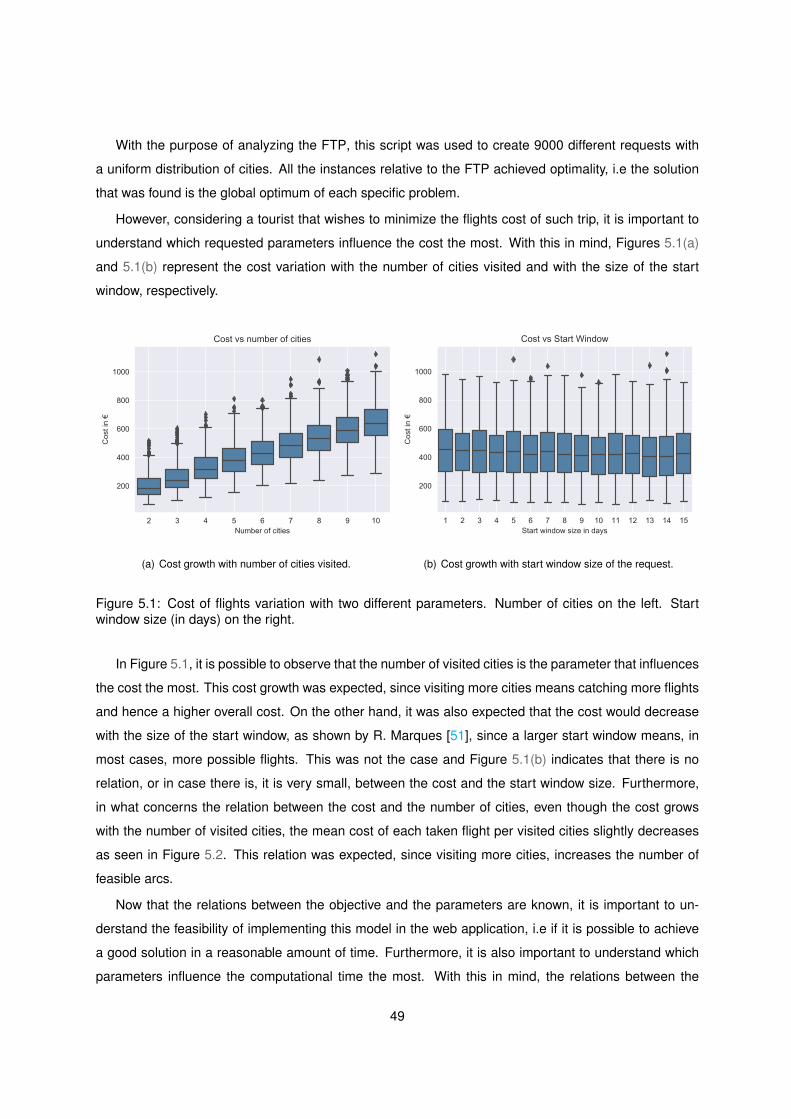
With the purpose of analyzing the FTP, this script was used to create 9000 different requests with

a uniform distribution of cities. All the instances relative to the FTP achieved optimality, i.e the solution

that was found is the global optimum of each specific problem.

However, considering a tourist that wishes to minimize the flights cost of such trip, it is important to

understand which requested parameters influence the cost the most. With this in mind, Figures 5.1(a)

and 5.1(b) represent the cost variation with the number of cities visited and with the size of the start

window, respectively.

2 3 4 5 6 7 8 9 10Number of cities

200

400

600

800

1000

Cos

t in

Cost vs number of cities

(a) Cost growth with number of cities visited.

1 2 3 4 5 6 7 8 9 10 11 12 13 14 15Start window size in days

200

400

600

800

1000

Cos

t in

Cost vs Start Window

(b) Cost growth with start window size of the request.

Figure 5.1: Cost of flights variation with two different parameters. Number of cities on the left. Startwindow size (in days) on the right.

In Figure 5.1, it is possible to observe that the number of visited cities is the parameter that influences

the cost the most. This cost growth was expected, since visiting more cities means catching more flights

and hence a higher overall cost. On the other hand, it was also expected that the cost would decrease

with the size of the start window, as shown by R. Marques [51], since a larger start window means, in

most cases, more possible flights. This was not the case and Figure 5.1(b) indicates that there is no

relation, or in case there is, it is very small, between the cost and the start window size. Furthermore,

in what concerns the relation between the cost and the number of cities, even though the cost grows

with the number of visited cities, the mean cost of each taken flight per visited cities slightly decreases

as seen in Figure 5.2. This relation was expected, since visiting more cities, increases the number of

feasible arcs.

Now that the relations between the objective and the parameters are known, it is important to un-

derstand the feasibility of implementing this model in the web application, i.e if it is possible to achieve

a good solution in a reasonable amount of time. Furthermore, it is also important to understand which

parameters influence the computational time the most. With this in mind, the relations between the

49


20

40

60

80

100

120

140

160

Cos

t in

Mean cost of each flight vs number of cities

Figure 5.2: Mean cost of flights taken per number of cities visited.

elapsed CPU time and the input parameters are depicted in Figure 5.3.


101

100

101

102

103

Elap

sed

CPU

tim

e in

sec

onds

[s]

Computational time growth with number of cities visited

(a) Computational time growth with the number of visitedcities (in a logarithmic scale).

1 2 3 4 5 6 7 8 9 10 11 12 13 14 15Start window size in days

0

200

400

600

800

1000

Elap

sed

CPU

tim

e in

sec

onds

[s]

Computational time growth with start window size

(b) Computational time variation with the size of the start win-dow in days.

Figure 5.3: Computational time analysis of the FTP.

Figure 5.3(a) shows an exponential growth of the computational time with the increase of the number

of visited cities, whilst Figure 5.3(b) illustrates a small linear growth of the computational time with the

increase of the start window size. This implies that, even though the computational time increases with

both parameters, the input that mostly influences the CPU time is the number of cities.

To evaluate whether or not this model is reliable on real time requests, the wall time should also be

computed. The wall time is the real time of the process and it is possible to find a relation between this

and the CPU time in normal conditions. This relation is illustrated in Figure 5.4 and one can observe that

most requests were answered in less than 10 seconds. In particular, 91.82% of the requests were an-

swered in less than 10 seconds and 99.07% in less than 20 seconds. This wall time is considerably lower

50

0 200 400 600 800 1000Elapsed CPU time in seconds [s]

0

10

20

30

40

50

60

70El

apse

d w

all t

ime

in s

econ

ds [s

]Elapsed wall time vs elapsed CPU time

Figure 5.4: Wall time compared to CPU time.

that the CPU time since CPLEX makes use of parallel computing and the server where the optimizations

were run has 16 cores each capable of running 2 threads simultaneously.

Moreover, since to the best of our knowledge the only work concerning the same exact problem is R.

Marques [3, 51], a more detailed comparison should be conducted as presented in Table 5.2.

Number of

cities visited2 3 4 5 6

SA 182.0 256.0 317.0 385.0 446.0Cost in eFTP ILP 182.0 (+ 0.0%) 240.0 (-6.25%) 313.0 (-1.26%) 375.0 (-2.60%) 428.0 (-4.03%)

SA 1.04 1.34 1.70 2.05 2.46Elapsed

CPU time [s] FTP ILP 0.83 (-20.19%) 2.78 (+107.46%) 4.53 (+164.47%) 5.43 (+164.87%) 7.95 (+223.17%)

SA 1.04 1.34 1.70 2.05 2.46Elapsed

Wall time [s] FTP ILP 0.24 (-77.04%) 0.33 (-75.27%) 0.43 (-74.84%) 0.52 (-74.81%) 0.69 (-71.87%)

Number of

cities visited7 8 9 10 Entire set

SA 502.5 560.5 604.5 665.0 62.37 per flightCost in eFTP ILP 486.0 (-3.28%) 535.0 (-4.56%) 591.0 (-2.23%) 638.0 (-4.06%) 60.27 per flight (-3.35%)

SA 2.88 3.38 3.88 4.39 2.46Elapsed

CPU time [s] FTP ILP 20.34 (+606.25%) 42.12 (+1146.15%) 82.67 (+2030.67%) 145.65 (+3217.77%) 8.23 (+234.86%)

SA 2.88 3.38 3.88 4.39 2.46Elapsed

Wall time [s] FTP ILP 1.60 (-44.70%) 3.69 (+8.79%) 7.02 (+80.54%) 11.20 (+154.32%) 0.70 (-71.80%)

Table 5.2: Comparison between the SA algorithm used by R.Marques [3, 51] and the FTP ILP formulation(solved with CPLEX) implemented in this work. For each number of cities, the results indicate themedian of the mean cost, elapsed CPU time and elapsed Wall time of each request. According to theexperiments described throughout this section.

51

Table 5.2 compares the formulation proposed in 3.1 with the Simulated Annealing (SA) optimization

algorithm used by R. Marques in [3, 51]. All the results in the table represent the median value of the

mean of each parameter. Three parameters are compared since we want to evaluate the response in

two ways. First, the main objective of each approach should be analyzed in order to understand if there

are significant improvements in using a complete method in this problem. Secondly, the feasibility of

applying these methods in a real-time web application needs to be assessed. For such purpose, both

the Elapsed CPU time and the Elapsed Wall time are evaluated. From Table 5.2 we can observe that

the achieved improvements in the cost come at the expense of a large increase in the Elapsed CPU

time. However, since CPLEX makes use of coarse grained parallel computing, the real computing time

in this machine largely decreases in normal conditions, outperforming the SA algorithm in most cases

of requests with less than seven cities.

These results emphasize that the SA algorithm is faster in achieving a good solution but cannot, in

most cases, find the optimal solution. On the other hand, using CPLEX, optimality was achieved at all

cases. Furthermore, considering the parallel computing capability of CPLEX, one concludes that this

method provides great advantages. With this in mind, the idea of using the result from the SA algorithm

to build an additional constraint for the ILP formulation, arised. The new constraint is hence written as:

csa(x) =

n∑i=0

n∑j=0

Iij∑k=1

cijkxijk ≤ SAsolution (5.1)

This constraint will act an aditional cut, during the B&C algorithm, and has the purpose of accelerating

the process. The whole data set of 9000 requests was analyzed. With this new ILP formulation, all

requests were solved to optimality. Nevertheless, this new formulation has the disadvantage of requiring

the SA solution beforehand. Figure 5.5 compares the new formulation with the FTP presented in 3.1.

From Figure 5.5(a), we can conclude that using the SA solution as an additional constraint to the ILP

formulation, the computational time required to solve the requests to optimality can be greatly reduced.

More specifically, the median of the global CPU time was enhanced in 70.80%. With this change, instead

of an increase of 2.35 times in the CPU time (vs the SA algorithm), the FTP only has an increase of

19.35%. However, because of the non-parallel implementation of the SA algorithm, when analyzing the

wall time, one observes that this parameter only presents improvements in requests of more than 8

cities, as seen in Figure 5.5(b). Hence, considering the fact that the prototype presented in Chapter 4 is

able to progressively update the responses to the end user, it is concluded that a good solution for large

requests is presenting the SA solution first. Then, use it as a constraint to the ILP formulation to search

for optimality to retrieve the final and optimal response.

Next, the results of the remaining variations of this model are presented, commented and compared

with the results shown in this section.

52


101

100

101

102

103

Elap

sed

CPU

tim

e in

sec

onds

[s]

Computational time gain of using the SA solution in the FTP

ModelFTPFTP with SA constraint

(a) Comparison of the computational time of the FTP vs theFTP with the SA solution as a constraint.


101

100

101

102

Elap

sed

Wal

l tim

e in

sec

onds

[s]

Wall time gain of using the SA solution in the FTP

ModelFTPFTP with SA constraint

(b) Comparison of the wall time of the FTP vs the FTP withthe SA solution as a constraint.

Figure 5.5: Impact of using the SA solution on the FTP formulation. The times relative to the FTP withSA constraint also include the time required to execute the SA algorithm.

5.2 Generalized Flying Tourist Problem

Similarly to what was described in Section 5.1, a script to construct 9000 random requests for the

analysis of this model was also implemented. The script respects the following rules:

• the requested trip must start and end in Lisbon,

• the tourist wishes to visit between two and nine clusters, each containing between two and five

cities,

• at each city, the user wishes a stop time between two and five days,

• the trip must start during the first fifteen days of October.

An additional restriction was considered by limiting the number of visited cities to 9, since at this point

some requests to visit 9 clusters could not be solved in less than 3600 CPU seconds. More specifically,

in 11.26% of the requests with 9 clusters, no solution was found in this time span. This corresponds to

1.32% of the total data set. Moreover, some other requests were also not solved to optimality in this time

span, as seen in Table 5.3. All the requests not shown in the table, with less than 6 clusters, were solved

to optimality in all cases.

It is now necessary to conduct an analysis of the impacts of this the modification of one of the

parameters and the addition of a new one, the number of cities and number of clusters respectively.

The number of cities is no longer equal to the number of cities visited. However, this parameter still

influences the size of the search space and hence, the computational time to solve the problem. On the

53

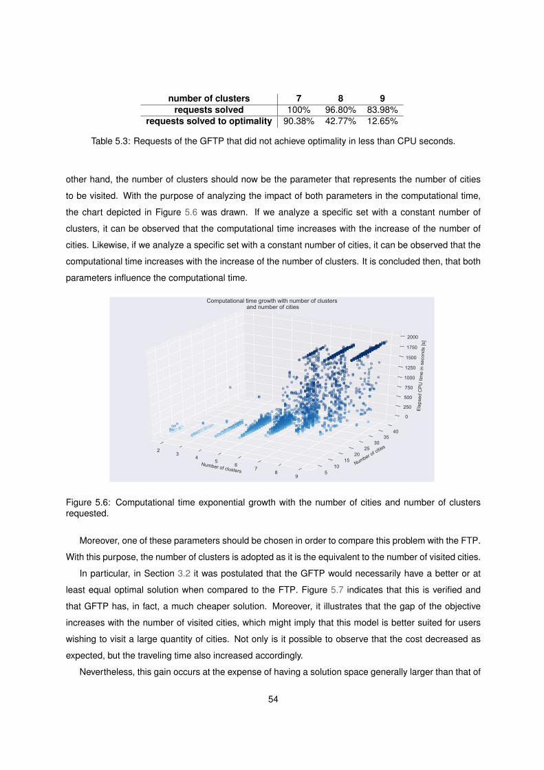
number of clusters 7 8 9requests solved 100% 96.80% 83.98%

requests solved to optimality 90.38% 42.77% 12.65%

Table 5.3: Requests of the GFTP that did not achieve optimality in less than CPU seconds.

other hand, the number of clusters should now be the parameter that represents the number of cities

to be visited. With the purpose of analyzing the impact of both parameters in the computational time,

the chart depicted in Figure 5.6 was drawn. If we analyze a specific set with a constant number of

clusters, it can be observed that the computational time increases with the increase of the number of

cities. Likewise, if we analyze a specific set with a constant number of cities, it can be observed that the

computational time increases with the increase of the number of clusters. It is concluded then, that both

parameters influence the computational time.

Number of clusters

23

45

67

89

Number of cities

510

1520

2530

3540

Elap

sed

CPU

tim

e in

sec

onds

[s]

0

250

500

750

1000

1250

1500

1750

2000

Computational time growth with number of clusters and number of cities

Figure 5.6: Computational time exponential growth with the number of cities and number of clustersrequested.

Moreover, one of these parameters should be chosen in order to compare this problem with the FTP.

With this purpose, the number of clusters is adopted as it is the equivalent to the number of visited cities.

In particular, in Section 3.2 it was postulated that the GFTP would necessarily have a better or at

least equal optimal solution when compared to the FTP. Figure 5.7 indicates that this is verified and

that GFTP has, in fact, a much cheaper solution. Moreover, it illustrates that the gap of the objective

increases with the number of visited cities, which might imply that this model is better suited for users

wishing to visit a large quantity of cities. Not only is it possible to observe that the cost decreased as

expected, but the traveling time also increased accordingly.

Nevertheless, this gain occurs at the expense of having a solution space generally larger than that of

54

2 3 4 5 6 7 8 9Number of cities

200

400

600

800

1000

Cos

t in

Cost of the FTP and GFTPvs number of cities

ModelFTPGFTP

(a) Cost growth with the number of cities visited of both theFTP and the GFTP.


0

2500

5000

7500

10000

12500

15000

17500

20000

Trav

elin

g tim

e [m

in]

Traveling time of the FTP and GFTP vs number of cities

ModelFTPGFTP

(b) Traveling time growth with the number of cities visited ofboth the FTP and the GFTP.

Figure 5.7: Objective function variation in the FTP and GFTP with the number of visited cities.

the FTP. For this reason, requesting large quantities of cities to be visited might lead to a computationally

heavy request. Figure 5.8 depicts that the exponential growth of the CPU time associated to this new

model has a larger growth ratio than that of the FTP ILP model.

5.3 Multi-Objective Flying Tourist Problem

This model was analyzed in 9000 different random requests that follow the same construction rules as in

Section 5.1 with the difference that now, instead of using the ILP formulation of the FTP, we use the multi-

objective formulation introduced in Section 3.3, the MO-FTP. This means that we are now optimizing

both the cost and the traveling time of the flights. We remind that we are using the CPLEX solver, which

has two options to approach the multi-objective optimization. The first option is a lexicographic multi-

objective optimization, where some objective functions are incomparably more important than others and

so, this optimization is processed in a sequential level of importance. The second option reduces the

multi-objective problem to a single-objective optimization through the merge of both objective functions

with the associated weights. Since the former implies a substantially greater optimization effort, the

computational time would substantially increase as two single-objective optimizations are performed.

For this reason, we only conduct the latter method, both in this section as well as in 5.4.

Consider a user that does not prioritize any of the objectives, i.e considers the cost and the traveling

time to be of the same importance when deciding on a trip. The weights of the objective functions were

not normalized since the trade-off between the cost and the traveling time is strictly subjective to each

user’s personal preference. Nonetheless, since the main objective of this formulation is to present the

improvements in terms of the traveling time when compared to the FTP, the used weights were both set

55


101

100

101

102

103

Elap

sed

CPU

tim

e in

sec

onds

[s]

Computational time variation of the FTP and GFTPvs number of cities visited

ModelFTPGFTP

Figure 5.8: Computational time exponential growth of both the FTP and the GFTP with the number ofvisited cities.

to the value 1. However, since magnitude of the traveling time of a flight (in minutes) is usually larger

than its cost (in euros), the traveling time presents as a larger term in the single-objective function.

Figure 5.9 illustrates the comparison of the results between the FTP and the MO-FTP, when consid-

ering both the cost and the traveling time objectives to have the same weight on the latter formulation.

In section 3.3, it was assumed that the MO-FTP would certainly achieve a better (or at least equal)

traveling time, when compared to the FTP. However, this improvement is achieved at the expense of

penalizing the flight cost. Figure 5.9 verifies these assumptions, and the average increase of 33.59%

in cost results, on average, on the reduction in 44.74% of the traveling time. Furthermore, since this

optimization treated both objective functions as a singular objective function, then the computational

time remains, approximately, the same as in the FTP, as clarified in Figure 5.10.

5.4 Multi-Objective Generalized Flying Tourist Problem

This formulation was used in 9000 random requests that follow the same construction rules as described

in Section 5.2. However, instead of utilizing the ILP formulation of the GFTP, we use the Multi-objective

formulation described in Section 3.4, the MO-GFTP.

Considering both the cost and the traveling time objective functions to be of the same importance,

56


0

200

400

600

800

1000

1200

1400

Cos

t in

Cost of the FTP and MO-FTP vs number of cities

ModelFTPMO-FTP

(a) Cost increase with the number of cities of both the FTPand the MO-FTP.


0

5000

10000

15000

20000

Trav

elin

g tim

e [m

in]


ModelFTPMO-FTP

(b) Traveling time increase with the number of cities of boththe FTP and the MO-FTP.

Figure 5.9: Objective function variation (cost on the left and traveling time on the right) in the FTP andMO-FTP with the number of cities. For the MO-FTP, both objectives have the same priority and weight.

they are given the same priority and hence, merged together.

Figure 5.11 depicts the comparison of the MO-GFTP with both the MO-FTP and the GFTP when

considering both objective functions to have the same weight. In Section 3.4, we theorized that the MO-

GFTP would attain the advantages of both the MO-FTP and the GFTP, i.e achieve better traveling times

through the multi-objective optimization, although not penalizing the flight cost as much by introducing

more arcs as a generalized, or set, problem. Figure 5.11 confirms these predictions. Furthermore,

the addition of more arcs, by using the MO-GFTP, allowed even better traveling times. However, the

results concerning the MO-GFTP take longer to process, since this is heavier computational problem.

Considering a timeframe of 3600 CPU seconds, a solution for 2.48% of the requests was not found and

5.08% of the results are not proved to be optimal.

Even though this is a multi-objective formulation (reduced to a single-objective problem), where both

objective functions have the same priority, it is possible to evaluate how the results vary with the weight

of each objective function. With this in mind, a Pareto front analysis was conducted. Consider a problem

consisting on 5 clusters, each with 5 cities and a stop time associated to each city of 3 days. For the

construction of the Pareto front, we use interval variations of the weight of both objective functions of

0.01. Naturally, since this variation is not introduced for every point in the infinite continuous domain of

possible weights, then the set of found solutions are merely an approximation of the Pareto Front and

the found points can be dominated by an unknown solution. However, this is improbable considering

that 100 different weights were considered. Considering that the traveling time function weight is given

by Weighttimef = 1−Weightcostf , Figure 5.12 illustrates the obtained approximation of the Pareto front.

The obtained approximation conveys only five points and suggest that at low traveling times, a small

57

2 3 4 5 6 7 8 9 10Number of cities visited

101

100

101

102

103

Elap

sed

CPU

tim

e in

sec

onds

[s]

Computational time variation of the FTP and MO-FTPvs number of cities visited

ModelFTPMO-FTP

Figure 5.10: Computational time exponential growth of both the FTP and the MO-FTP with the numberof cities. For the MO-FTP, the objectives (cost and traveling time) have the same priority and weight.

2 3 4 5 6 7 8 9Number of cities visited

0

200

400

600

800

1000

1200

1400

Cos

t in

Cost of the MO-FTP, GFTP and MO-GFTPvs number of cities visited

ModelMO-FTPGFTPMO-GFTP

(a) Cost growth with the number of cities of the GFTP, theMO-FTP and the MO-GFTP.


0

2000

4000

6000

8000

10000

12000

14000

Trav

elin

g tim

e [m

in]


ModelMO-FTPGFTPMO-GFTP

(b) Traveling time growth with the number of cities of theGFTP, the MO-FTP and the MO-GFTP.

Figure 5.11: Objective function variation, cost on the left and traveling time on the right, in the GFTP, theMO-FTP and the MO-GFTP with the number of cities. For the MO-FTP and MO-GFTP, both objectiveshave the same priority and weight.

improvement in this objective implies a large increase in cost. Likewise, at low costs, a small improve-

ment in this objective implies a large increase in traveling time.

58

200 250 300 350 400 450Cost in

1500

2000

2500

3000

3500

4000

4500

5000Tr

avel

ing

time

in s

econ

ds [s

]Pareto front of a MO-GFTP problem

Cost function weight1.000.990.97 - 0.980.36 - 0.960.00 - 0.35

Figure 5.12: Obtained approximation of Pareto front of a MO-GFTP considering 5 clusters and 5 citiesper cluster.

5.5 Summary

The foregoing chapter presents an evaluation of the models presented in Chapter 3. In Section 5.1,

we introduced the overall results of the an ILP formulation of FTP concluding that the number of cities

visited is the parameter that influences this formulation the most. We then compare the results of this

optimization method with the SA algorithm used by R. Marques [51] and conclude that this formulation

presents advantages and disadvantages versus the stochastic method. Even though it always achieves

optimality, this comes at the expense of larger computational times. With this in mind, we implemented

an optimization method that finds the aimed solution in a sequential manner, i.e first we solve the problem

with the SA algorithm and use the solution retrieved as a constraint to the ILP formulation, which reduces

the computational time to reach optimality. Next, we demonstrate that the results predicted for the

Cost per flight [e] Traveling time per flight [min]

FTP 60.27 912.82GFTP 30.71 (-46.2%) 533.87 (-41.5%)MO-FTP 75.20 (+24.8%) 435.81 (-52.3%)MO-GFTP 45.83 (-24.0%) 179.33 (-80.4%)

Table 5.4: Comparison of the objective results of the aforementioned models. The results indicate themedian, per flight taken, of the mean cost and traveling time of each request.

59

considered variations of the FTP are verified. Table 5.4 resumes and compares the median of the

results of the proposed models. First, the GFTP presents great improvements both in the cost and in

the traveling time. For this reason this model is ideal in case the end user wishes to reduce both of

these parameters. Second, if the end user wishes to maintain the original set of cities but wishes to save

traveling time at the expense of an increase in cost, the MO-FTP is recommended. Lastly, if the traveling

time of the GFTP is still not the desirable, then the MO-GFTP joins both benefits.

60

6Conclusions

Contents6.1 Summary . . . . . . . . . . . . . . . . . . . . . . . . . . . . . . . . . . . . . . . . . . . . 626.2 Future Work . . . . . . . . . . . . . . . . . . . . . . . . . . . . . . . . . . . . . . . . . . 63

61

6.1 Summary

The increase on flights over the last decade has posed several new challenges. A vast variety of online

travel agencies have started to attempt to make flight choices easier for the users. A large quantity

of these web services already offer simple solutions as finding an optimal tour connecting two cities.

Nonetheless, the ways of traveling have changed throughout the last two decades [1]. Nowadays, flying

has become a common and affordable means of transportation and travelers have today very different

purposes for flying. Therefore, these web applications have started to tailor their services in order to

provide new creative services that fit every user’s needs. Throughout this work, we developed different

models that shape peculiar situations we believe to be of the user’s interest.

When accounting for more complex problems, for instance an unconstrained multi-city search, these

search engines aim to present solutions in a small time frame. Notwithstanding, this implies the use

of incomplete methods and therefore there is no guarantee that these solutions are optimal. With this

in mind, the main contributions of this work were the formulations of complete methods to assure the

quality of four different scenarios:

1. The Flying Tourist Problem, which minimizes the total flight cost or traveling time of an end user

wishing to visit multiple cities in no preemptive order.

2. The Generalized Flying Tourist Problem, that minimizes the total flight cost or traveling time of an

end user wishing to visit one city per cluster, having multiple cluster in no prescribed order.

3. The Multi-objective Flying Tourist Problem, that aims to optimize a trade-off between the total flight

cost and traveling time of the Flying Tourist Problem.

4. The Multi-objective Generalized Flying Tourist Problem, which optimizes the total flight cost and

traveling time of the Generalized Flying Tourist Problem.

After the problem statements, Integer Linear Programming (ILP) formulations for each of the prob-

lems were proposed and implemented using a commercial solver, CPLEX, as an optimization module.

This module was later integrated in a web application previously developed by R.Marques [51] in order to

solve real world complex routing problems. This application was subject to several design modifications

to adapt it to the new proposed models.

The results of the ILP formulation of the FTP were compared to an incomplete method, the Simu-

lated Annealing (SA) algorithm. The complete method used in this work outperformed the SA algorithm

in what concerns the solution, since it consistently found an optimal solution in less than 1800 seconds

for a maximum of ten cities. Moreover, even though the ILP formulation involved larger computational

optimization times, this method outperformed the SA algorithm in what concerns the wall clock opti-

mization time for less than eight cities. Comparing the other formulations with the obtained results of

62

the FTP, we concluded that the GFTP managed to consistently reduce the total flight cost in half, the

MO-FTP achieved a large reduction in the traveling time at the expense of the total flight cost and finally,

the MO-GFTP attained both benefits.

6.2 Future Work

Considering that the work developed proposes to resolve complex routing problems in near real-time,

there is the need to consistently improve and find innovative techniques for the foregoing system.

• Considering the FTP, we suggest the integration of other means of transportation such as buses

or trains. We believe that this solution starts by constructing a database, for instance with the

software MongoDB. This strategy could also improve the efficiency of the data acquisition system.

• Since the developed optimization modules of the GFTP, MO-FTP and MO-GFTP only comprise

complete methods, the first answer provided to the Client Side Application will take a long time. To

negate this, we suggest the implementation of heuristics and meta-heuristics to be solved before

the formulations here presented so that solutions are given in a sequential manner to the user.

• Considering the multi-objective formulations we recommend exploring the multi-objective evolu-

tionary algorithms in order to compare the quality of the solutions here presented. With this in

mind we suggest using framework MOEA/D and the NSGA II Algorithm.

63

Bibliography

[1] International Air Transport Association Annual Review 2019. 75th Annual General Meeting, Seoul,

June 2019, . Accessed October 2019.

[2] Kiwi.com API documentation. https://docs.kiwi.com/, . Accessed October 2019.

[3] Nuno Roma Rafael Marques, Luıs M. S. Russo. Flying tourist problem: Flight time and cost mini-

mization in complex routes. Expert Systems with Applications, 130:172 – 187, September 2019.

[4] George B. Dantzig, Delbert Ray Fulkerson, and Selmer M. Johnson. Solution of a large-scale

traveling-salesman problem. In 50 Years of Integer Programming, 1954.

[5] Christos Papadimitriou and Kenneth Steiglitz. Combinatorial Optimization: Algorithms and Com-

plexity, volume 32. 01 1982. ISBN 0-13-152462-3. doi: 10.1109/TASSP.1984.1164450.

[6] Alexander Schrijver. Algorithms and Combinatorics. Springer Science+Business Media, 2008.

ISBN 3540204563. doi: 10.1007/978-3-642-24508-4.

[7] George L. Nemhauser Laurence A. Wolsey. Integer and Combinatorial Optimization, volume 1.

John Wiley & Sons, Inc., 1988.

[8] Gilbert Laporte, Helene Mercure, and Yves Nobert. Generalized travelling salesman problem

through n sets of nodes: the asymmetrical case. Discrete Applied Mathematics, 18(2):185–197,

1987. ISSN 0166218X. doi: 10.1016/0166-218X(87)90020-5.

[9] Roy Jonker and Ton Volgenant. Transforming asymmetric into symmetric traveling salesman

problems: erratum. Operations Research Letters, 5(4):215–216, 1983. ISSN 01676377. doi:

10.1016/0167-6377(86)90081-7.

[10] Holger H. Hoos and Thomas Stutzle. Stochastic Local Search Foundations and Applications. 1:

658, 2004.

[11] Gregory Gutin and Abraham P. Punnen. The Traveling Salesman Problem and its Variations, vol-

ume 1. Springer US, 2007. ISBN 978-0-306-48213-7. doi: 10.1007/b101971.

65

[12] E. L. Lawler, Jan Karel Lenstra, A. H. G. Rinnooy Kan, and D. B. Shmoys. The Traveling Salesman

Problem: A Guided Tour of Combinatorial Optimization, volume 1. John Wiley & Sons, Inc., 1985.

ISBN 978-0-471-90413-7.

[13] Roberto Roberti and Paolo Toth. Models and algorithms for the Asymmetric Traveling Salesman

Problem: an experimental comparison. EURO Journal on Transportation and Logistics, 1(1):113–

133, 2012. ISSN 2192-4376. doi: 10.1007/s13676-012-0010-0.

[14] C. E. Miller, A. W. Tucker, and R. A Zemlin. Integer Programming Formulation of Traveling Salesman

Problems. Journal of the ACM, 7:326–329, 1960. ISSN 00045411. doi: 10.1145/321043.321046.

[15] Bezalel Gavish and Stephen C. Graves. The Travelling Salesman Problem and Related Problems.

Operations Research Center Working Papers, 1978.

[16] M. Desrochers and G. Laporte. Improvements and extensions to the Miller–Tucker–Zemlin subtour

elimination constraints. Operations Research Letters, 10(1):27—-36, 1991. doi: https://doi.org/10.

1016/0167-6377(91)90083-2.

[17] K.R Fox. Production scheduling on parallel lines with dependencies. PhD thesis, Johns Hopkins

University, 1973.

[18] Kenneth Fox, Bezalel Gavish, and Stephen Graves. An n-constraint formulation of the (time-

dependent) traveling salesman problem. Operations Research, 28:1018–1021, August 1980. doi:

10.1287/opre.28.4.1018.

[19] Jean Claude Picard and Maurice Queyranne. Time-Dependent Traveling Salesman Problem and

Its Application To the Tardiness Problem in One-Machine Scheduling. Operations Research, 26(1):

86–110, 1978. ISSN 0030364X. doi: 10.1287/opre.26.1.86.

[20] Ulrich Pferschy and Rostislav Stanek. Generating subtour elimination constraints for the tsp from

pure integer solutions. Central European Journal of Operations Research, 25(1):231–260, March

2017. ISSN 1613-9178. doi: 10.1007/s10100-016-0437-8. URL https://doi.org/10.1007/

s10100-016-0437-8.

[21] Louis Philippe Bigras, Michel Gamache, and Gilles Savard. The time-dependent traveling salesman

problem and single machine scheduling problems with sequence dependent setup times. Discrete

Optimization, 5(4):685–699, 2008. ISSN 15725286. doi: 10.1016/j.disopt.2008.04.001.

[22] Norbert Ascheuer, Matteo Fischetti, and Martin Grotschel. A polyhedral study of the asymmetric

traveling salesman problem with time windows. Networks, 36(2):69–79, 2000. ISSN 00283045.

doi: 10.1002/1097-0037(200009)36:2〈69::AID-NET1〉3.0.CO;2-Q.

66

https://doi.org/10.1007/s10100-016-0437-8

https://doi.org/10.1007/s10100-016-0437-8

[23] Charles E. Noon and James C. Bean. A Lagrangian Based Approach for the Asymmetric General-

ized Traveling Salesman Problem. Operations Research, 39(4):623–632, 1991. ISSN 0030-364X.

doi: 10.1287/opre.39.4.623.

[24] Petrica C. Pop. New integer programming formulations of the generalized travelling salesman

problem. American Journal of Applied Sciences, 4(11):932–937, 2007. ISSN 15543641. doi:

10.3844/ajassp.2007.932.937.

[25] E. L. Ulungu and J. Teghem. Multi-objective combinatorial optimization problems: A survey. Jour-

nal of Multi-Criteria Decision Analysis, 3(2):83–104, 1994. ISSN 10991360. doi: 10.1002/mcda.

4020030204.

[26] David A. Van Veldhuizen and Gary B. Lamont. Multiobjective evolutionary algorithms: Analyzing

the state-of-the-art. Evolutionary Computation, 8(2):125–147, June 2000. ISSN 1063-6560. doi:

10.1162/106365600568158.

[27] Luis Paquete, Marco Chiarandini, and Thomas Stutzle. Pareto Local Optimum Sets in the Biobjec-

tive Traveling Salesman Problem: An Experimental Study. In Xavier Gandibleux, Marc Sevaux, Ken-

neth Sorensen, and Vincent T’kindt, editors, Metaheuristics for Multiobjective Optimisation, pages

177–199. Springer Berlin Heidelberg, 2004. doi: 10.1007/978-3-642-17144-4 7.

[28] J. E. Kelley. The cutting-plane method for solving convex programs. Journal of the Society for

Industrial and Applied Mathematics, 8(4):703–712, 1960. ISSN 03684245. URL http://www.

jstor.org/stable/2099058.

[29] E. Mitchell John. Integer programming: Branch and cut algorithms. In Encyclopedia of Optimization

2nd Edition, pages 1643–1649. Springer, 2009.

[30] Ralph E. Gomory. Outline of an algorithm for integer solutions to linear programs. Bull. Amer.

Math. Soc., 64(5):275–278, September 1958. URL https://projecteuclid.org:443/euclid.

bams/1183522679.

[31] J. N. Hooker. Integer programming duality. In Encyclopedia of Optimization 2nd Edition, pages

1657–1667. Springer, 2009.

[32] E. Mitchell John. Integer programming. In Encyclopedia of Optimization 2nd Edition, pages 1650–

1657. Springer, 2009.

[33] E. Mitchell John. Integer programming: Branch and bound methods. In Encyclopedia of Optimiza-

tion 2nd Edition, pages 1634–1643. Springer, 2009.

67

http://www.jstor.org/stable/2099058

http://www.jstor.org/stable/2099058

https://projecteuclid.org:443/euclid.bams/1183522679

https://projecteuclid.org:443/euclid.bams/1183522679

[34] M. W. P. Savelsbergh. Preprocessing and Probing Techniques for Mixed Integer Programming

Problems. ORSA Journal on Computing, 6(4):445–454, 1994. ISSN 0899-1499. doi: 10.1287/ijoc.

6.4.445.

[35] Emile Aarts, Jan Korst, and Wil Michiels. Simulated Annealing, pages 187–210. Number 1999.

Springer US, 2005. ISBN 978-0-387-23460-1. doi: 10.1007/0-387-28356-0 7.

[36] Zakir Ahmed. The ordered clustered travelling salesman problem: A hybrid genetic algorithm. The

Scientific World Journal, 2014:13, 2014. doi: 10.1155/2014/258207.

[37] N. Karmakar. A New Polynomial-Time Algorithm for Linear Programming. Combinatorica”, 4:373–

395, 1984. ISSN 1439-6912. doi: 10.1007/BF02579150.

[38] Jens Clausen. Branch and bound algorithms-principles and examples, 1999.

[39] Hans D. Mittelmann. Benchmarks for optimization software. Accessed 7 Sep. 2019.

[40] ILOG IBM CPLEX, Copyright c© 2019. https://www.ibm.com/analytics/cplex-optimizer, . Accessed

October 2019.

[41] Bernhard Meindl and Matthias Templ. Analysis of commercial and free and open source solvers

for linear optimization problems. ESSnet on commom tools and harmonised methodology for

SDC in the ESS, 1(1):1–14, 2012. ISSN 18885063. URL http://www.statistik.tuwien.ac.

at/forschung/CS/CS-2012-1complete.pdf---.

[42] Copyright c© 2019 Gurobi Optimization, LLC. Gurobi 8 performance benchmarks, February 2019.

[43] David S. Johnson and Lyle A. McGeoch. The traveling salesman problem: a case study, pages

215–310. John Wiley & Sons, Inc., 1995. doi: 10.1515/9780691187563-011.

[44] Christian Nilsson. Heuristics for the traveling salesman problem. 2003.

[45] B. Golden, L. Bodin, T. Doyle, and W. Stewart. Approximate traveling salesman algorithms. Oper-

ations Research, 28(3):694–711, 1980. ISSN 0030364X, 15265463.

[46] Author S Lin and B W Kernighan. An Effective Heuristic Algorithm for the Traveling-Salesman

Problem. Operations Research, 21(2):498–516, 1971.

[47] Ibrahim Osman and James Kelly. Meta-Heuristics: Theory and Applications. Springer US, 01 1996.

ISBN 978-1-4612-8587-8. doi: 10.1007/978-1-4613-1361-8.

[48] J.-L. Deneubourg, S. Aron, L S. Goss, and J. M. Pasteels L. The Self-Organizing Exploratory

Pattern of the Argentine Ant. Journal of insect behavior, 3(2):159–168, 1989. ISSN 08927553. doi:

10.1007/BF01417909. URL http://link.springer.com/article/10.1007/BF01417909.

68

http://www.statistik.tuwien.ac.at/forschung/CS/CS-2012-1complete.pdf---

http://www.statistik.tuwien.ac.at/forschung/CS/CS-2012-1complete.pdf---

http://link.springer.com/article/10.1007/BF01417909

[49] Marco Dorigo and Luca Maria Gambardella. Ant colonies for the travelling salesman problem.

BioSystems, 43(2):73–81, 1997. ISSN 03032647. doi: 10.1016/S0303-2647(97)01708-5.

[50] H.H. Hoos and T. Stutzle. MAX MIN Ant System. Future Generation Computer Systems, 16(June):

889–914, 1999.

[51] Rafael Marques. Flight Time and Cost Minimization in Complex Routes. Master’s thesis, Universi-

dade de Lisboa, Instituto Superior Tecnico, October 2018.

[52] Xiang Li, Jiandong Zhou, and Xiande Zhao. Travel itinerary problem. Transportation Research Part

B Methodological, 91:332–343, May 2016. doi: 10.1016/j.trb.2016.05.013.

[53] Imdat Kara, Huseyin Guden, and Ozge N. Koc. New formulations for the generalized traveling

salesman problem. In Proceedings of the 6th International Conference on Applied Mathemat-

ics, Simulation, Modelling, ASM’12, pages 60–65, Stevens Point, Wisconsin, USA, 2012. World

Scientific and Engineering Academy and Society (WSEAS). ISBN 978-1-61804-076-3. URL

http://dl.acm.org/citation.cfm?id=2209505.2209517.

[54] React, Copyright c© 2019 Facebook Inc. https://www.react.org, . Accessed October 2019.

[55] Redux.io Copyright c© 2018, LLC. https://redux.io, . Accessed October 2019.

[56] Python, Copyright c©2001-2019. Python Software Foundation. https://www.python.org, . Accessed

October 2019.

[57] Heroku, Copyright c© 2019 Salesforce.com. https://www.heroku.com, . Accessed October 2019.

[58] Node JS, Copyright c© Node.js Foundation. https://nodejs.org/en/, . Accessed October 2019.

[59] Django Project, Copyright c© 2005-2019 Django Software Foundation and individual contributors.

https://www.djangoproject.com, . Accessed October 2019.

69

http://dl.acm.org/citation.cfm?id=2209505.2209517

flying tourist problem - ulisboa

Documents