fmm tutorial

8/2/2019 FMM Tutorial

http://slidepdf.com/reader/full/fmm-tutorial 1/14

A short primer on the fast multipole method

VIKAS CHANDRAKANT RAYKAR

University of Maryland, CollegePark

[email protected]

This is intended to be a short tutorial on fast multipole methods (FMM). These were mainlywritten to ease my understanding of the subject. We discuss the main technical concepts likesingular potentials, factorization, and translation. Important topics like error analysis and thecomputational cost analysis are left out. The single level FMM is discussed in detail since the fastGauss transform is based on the single level FMM. A brief discussion of multiple level FMM isgiven at the end. This primer is mainly based on the course offered by Dr. Ramani Duraiswamiand Dr. Nail Gumerov at the University of Maryland, College Park.

[ FMM tutorial ]: April 8, 2006

Contents

1 Introduction 2

2 Potentials and Factorization 32.1 Regular (Local) Expansion: R-expansion . . . . . . . . . . . . . . . . 32.2 Far Field Expansion: S-expansion . . . . . . . . . . . . . . . . . . . . 52.3 Why R- and S-expansions? . . . . . . . . . . . . . . . . . . . . . . . 6

3 Middleman method 6

3.1 For regular potentials . . . . . . . . . . . . . . . . . . . . . . . . . . 63.2 For singular potentials . . . . . . . . . . . . . . . . . . . . . . . . . . 7

4 Translations (Re-expansions) 84.1 R|R re-expansion (Local to Local) . . . . . . . . . . . . . . . . . . . 94.2 S|S re-expansion (Multipole to Multipole) . . . . . . . . . . . . . . . 94.3 S|R re-expansion (Multipole to Local) . . . . . . . . . . . . . . . . . 94.4 R|S re-expansion (Local to Multipole) . . . . . . . . . . . . . . . . . 10

5 Single Level FMM 115.1 What is the problem with middleman ? . . . . . . . . . . . . . . . . 115.2 Space subdivison . . . . . . . . . . . . . . . . . . . . . . . . . . . . . 115.3 R expansion . . . . . . . . . . . . . . . . . . . . . . . . . . . . . . . . 125.4 S expansion . . . . . . . . . . . . . . . . . . . . . . . . . . . . . . . . 125.5 S|R Translation . . . . . . . . . . . . . . . . . . . . . . . . . . . . . . 13

6 Multi level FMM 13

FMM tutorial April 8, 2006



2 · Vikas Chandrakant Raykar

1. INTRODUCTION

The fast multipole method has been called one of the ten most significant algorithms[Dongarra and Sullivan 2000][Board and Schulten 2000] in scientific computationdiscovered in the 20th century, and won its inventors, Vladimir Rokhlin and LeslieGreengard, the 2001 Steele prize, in addition to getting Greengard the ACM 1987best dissertation award [Greengard 1988].

The algorithm allows the product of particular structured dense matrices witha vector to be evaluated approximately in O(N ) or O(N log N ) operations, whendirect multiplication requires O(N 2) operations. Coupled with advances in itera-tive methods for the solution of linear systems, they provide O(N ) or O(NlogN )time and memory complexity solutions of problems that hitherto required O(N 3)or O(N 2) time complexity and O(N 2) memory complexity. For extremely largeproblems, the gain in efficiency and memory can be very significant, and enablesthe use of more sophisticated modeling approaches that, while known to be better,

may have been discarded as computationally infeasible in the past.Originally this method was developed for the fast summation of the potential

fields generated by a large number of sources (charges), such as those arising ingravitational or electrostatic potential problems, that are described by the Laplaceequation in two or three dimensions [Greengard and Rokhlin 1987]. This lead to thename for the algorithm. Since then FMM has also found application in many otherproblems, e.g. in non-parametric statistics, finance, chemistry, machine learning,computer vision etc.

We are interested in computing the following sum

vj =N i=1

qiΦ(yj , xi), j = 1, . . . , M , (1)

where

—xi ∈ Rdi=1,...,N are called the source points,

—yj ∈ Rdj=1,...,M are called the target points,

—qi ∈ Ri=1,...,N are the source weights,

—and Φ is the potential function.

Φ(yj , xi) is the contribution of source at xi towards the target point yj. Thecomputational complexity to directly evaluate Eq. 1 is O(M N ).

The fast multipole methods look for computation of the same problem with com-plexity O(M +N ) and error < . The FMM represents a fundamental change in theway of designing numerical algorithms, in that it solves the problem approximately,

and trades complexity for exactness. However, practically this distinction is usuallynot important, as in general, we need the solution to any scientific problem onlyto a specified accuracy, and in any case the accuracy specified to the FMM can bearbitrary. In the case when the error of the FMM does not exceed the machineprecision error there is no difference between the exact and approximate solution.

Compared to the FFT, the FMM does not require that the data be uniformlysampled, and in general it does not rely on discretization structure to achieve thespeedup.




Not all those that wander are lost -J.R.R. Tolkien. · 3

x∗

xi

y

r∗

1

(a)

x∗

xi

y

r∗

1

(b)

x∗

xi

y

r∗

1

(c)

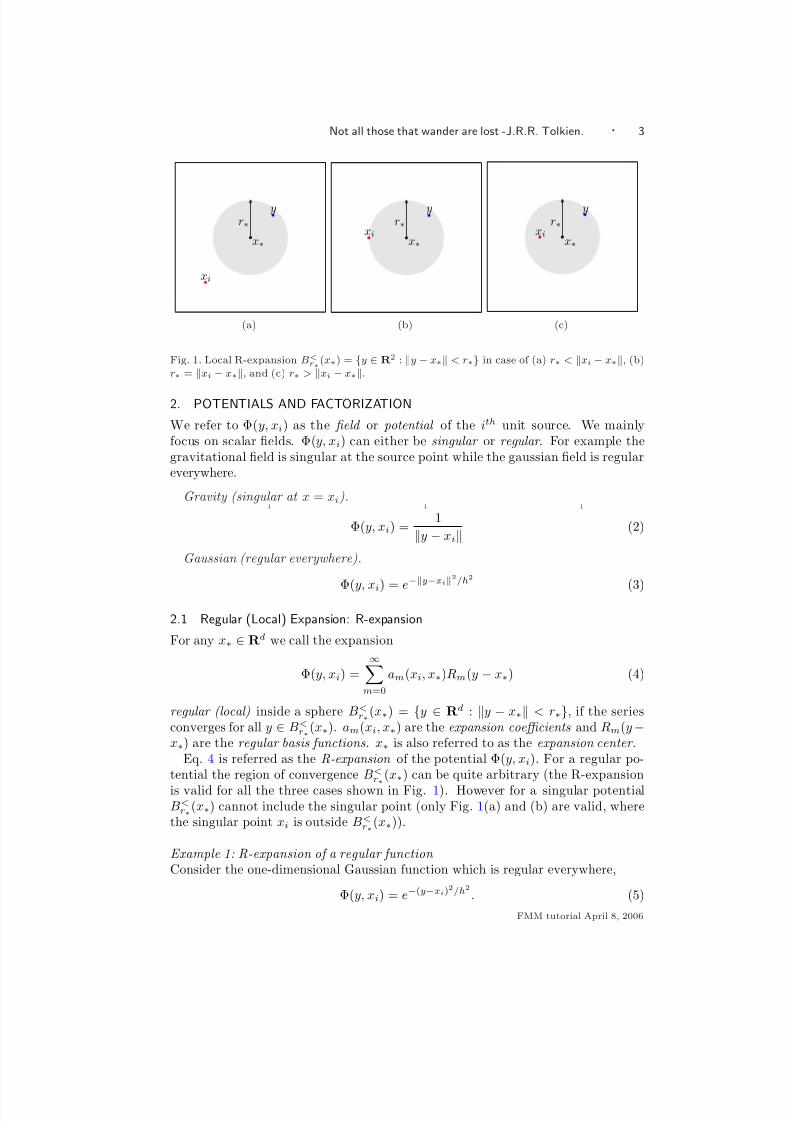
Fig. 1. Local R-expansion B<r∗

(x∗) = y ∈ R2 : y − x∗ < r∗ in case of (a) r∗ < xi − x∗, (b)r∗ = xi − x∗, and (c) r∗ > xi − x∗.

2. POTENTIALS AND FACTORIZATION

We refer to Φ(y, xi) as the field or potential of the ith unit source. We mainlyfocus on scalar fields. Φ(y, xi) can either be singular or regular . For example thegravitational field is singular at the source point while the gaussian field is regulareverywhere.

Gravity (singular at x = xi).

Φ(y, xi) =1

y − xi(2)

Gaussian (regular everywhere).

Φ(y, xi) = e

−y−xi2/h2

(3)

2.1 Regular (Local) Expansion: R-expansion

For any x∗ ∈ Rd we call the expansion

Φ(y, xi) =∞

m=0

am(xi, x∗)Rm(y − x∗) (4)

regular (local) inside a sphere B<r∗(x∗) = y ∈ Rd : y − x∗ < r∗, if the series

converges for all y ∈ B<r∗(x∗). am(xi, x∗) are the expansion coefficients and Rm(y −

x∗) are the regular basis functions. x∗ is also referred to as the expansion center .Eq. 4 is referred as the R-expansion of the potential Φ(y, xi). For a regular po-

tential the region of convergence B<r∗

(x∗) can be quite arbitrary (the R-expansion

is valid for all the three cases shown in Fig. 1). However for a singular potentialB<r∗(x∗) cannot include the singular point (only Fig. 1(a) and (b) are valid, where

the singular point xi is outside B<r∗

(x∗)).

Example 1: R-expansion of a regular function Consider the one-dimensional Gaussian function which is regular everywhere,

Φ(y, xi) = e−(y−xi)2/h2 . (5)





For any x∗ ∈ R and y − x∗ < r∗ < ∞, making use of the Taylor’s series, theR-expansion can be written as follows.

Φ(y, xi) = e−[(y−x∗)−(xi−x∗)]2/h2

= e−(y−x∗)2/h2e−(xi−x∗)2/h2e2(y−x∗)(xi−x∗)/h2

= e−(y−x∗)2/h2e−(xi−x∗)2/h2∞

m=0

2m

m!

y − x∗

h

mxi − x∗

h

m=

∞m=0

2m

m!e−(xi−x∗)2/h2

xi − x∗

h

me−(y−x∗)2/h2

y − x∗

h

m=

∞m=0

am(xi, x∗)Rm(y − x∗), (6)

where

am(xi, x∗) = 2m

m!e−(xi−x∗)2/h2 xi − x∗

hm

. (7)

Rm(y − x∗) = e−(y−x∗)2/h2

y − x∗

h

m. (8)

Example 2: R-expansion of a singular function.Consider the one-dimensional gravitational field which is singular at y = xi,

Φ(y, xi) =1

y − xi. (9)

For any x∗ ∈ R and y − x∗ < r∗ ≤ xi − x∗ (to make sure we do not includethe singular point xi), [We make use of the Geometric progression.]

Φ(y, xi) =1

(y − x∗) − (xi − x∗)= −

1

(xi − x∗)[1 − y−x∗xi−x∗

]

= −1

(xi − x∗)

1 −

y − x∗

xi − x∗

−1

= −1

(xi − x∗)

∞m=0

(y − x∗)m

(xi − x∗)m, sincey − x∗ < xi − x∗

=∞

m=0

−1

(xi − x∗)m+1

(y − x∗)m

=

∞m=0

am(xi, x∗)Rm(y − x∗), (10)

where

am(xi, x∗) =−1

(xi − x∗)m+1. (11)

Rm(y − x∗) = (y − x∗)m. (12)





x∗

xi

y

R∗

1

(a)

x∗xi

y

R∗

1

(b)

x∗xi

y

R∗

1

(c)

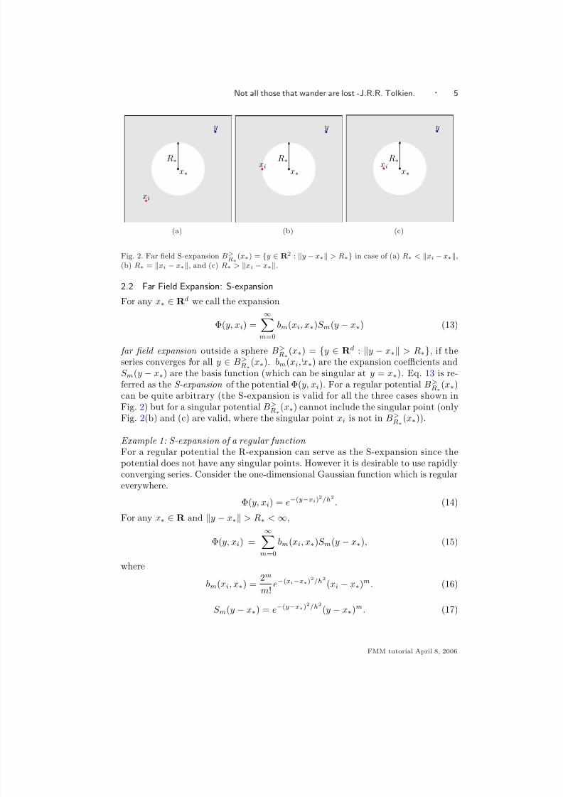
Fig. 2. Far field S-expansion B>

R∗(x∗) = y ∈ R

2 : y −x∗ > R∗ in case of (a) R∗ < xi −x∗,(b) R∗ = xi − x∗, and (c) R∗ > xi − x∗.

2.2 Far Field Expansion: S-expansion

For any x∗ ∈ Rd we call the expansion

Φ(y, xi) =

∞m=0

bm(xi, x∗)S m(y − x∗) (13)

far field expansion outside a sphere B>R∗

(x∗) = y ∈ Rd : y − x∗ > R∗, if theseries converges for all y ∈ B>

R∗

(x∗). bm(xi, x∗) are the expansion coefficients andS m(y − x∗) are the basis function (which can be singular at y = x∗). Eq. 13 is re-ferred as the S-expansion of the potential Φ(y, xi). For a regular potential B>

R∗

(x∗)can be quite arbitrary (the S-expansion is valid for all the three cases shown inFig. 2) but for a singular potential B>

R∗

(x∗) cannot include the singular point (only

Fig. 2(b) and (c) are valid, where the singular point xi is not in B>R∗(x∗)).

Example 1: S-expansion of a regular function For a regular potential the R-expansion can serve as the S-expansion since thepotential does not have any singular points. However it is desirable to use rapidlyconverging series. Consider the one-dimensional Gaussian function which is regulareverywhere.

Φ(y, xi) = e−(y−xi)2/h2 . (14)

For any x∗ ∈ R and y − x∗ > R∗ < ∞,

Φ(y, xi) =

∞

m=0

bm(xi, x∗)S m(y − x∗), (15)

where

bm(xi, x∗) =2m

m!e−(xi−x∗)2/h2(xi − x∗)m. (16)

S m(y − x∗) = e−(y−x∗)2/h2(y − x∗)m. (17)





Example 2: S-expansion of a singular function.Consider the one-dimensional gravitational field which is singular at y = xi,

Φ(y, xi) =1

y − xi=

∞m=0

bm(xi, x∗)S m(y − x∗), . (18)

For any x∗ ∈ R and y − x∗ > R∗ ≥ xi − x∗ (to make sure we do not includethe singular point xi),

Φ(y, xi) =1

(y − x∗) − (xi − x∗)=

1

(y − x∗)[1 − xi−x∗y−x∗

]

=1

(y − x∗)

1 −

xi − x∗

y − x∗

−1

=1

(y − x∗)

∞m=0

(xi − x∗)m

(y − x∗)m

=

∞m=0

1

(y − x∗)m+1 (xi − x∗)m

=

∞m=0

bm(xi, x∗)S m(y − x∗), (19)

where,

bm(xi, x∗) = (xi − x∗)m, S m(y − x∗) =1

(y − x∗)m+1. (20)

2.3 Why R- and S-expansions?

If the potential has a singular point xi, then we use R-expansion for all y − x∗ <

xi − x∗, and S-expansion for all y − x∗ > xi − x∗. Note that the singular

point xi is at the boundary of the regions for R- and S-expansions. Also in case of regular potentials depending upon how far y is from x∗ either the S-expansion orthe R-expansion will converge much more rapidly than the other.

3. MIDDLEMAN METHOD

3.1 For regular potentials

Consider a potential which is regular everywhere. Then we can use the R-expansionabout a point x∗ for factorizing the potential. The field at yj can be evaluated asfollows.

vj =

N i=1

qiΦ(yj , xi)

=N i=1

qi ∞m=0

am(xi, x∗)Rm(yj − x∗) [R-expansion]

=N i=1

qi

p−1m=0

am(xi, x∗)Rm(yj − x∗) + error( p, xi, yj , x∗)

(21)

The truncation number p is chosen based on the desired error. One of the trickiestpart in designing a good FMM algorithm lies in getting a pretty tight bound for





1

(a)

1

(b)

1

(c)

1

(d)

1

(e)

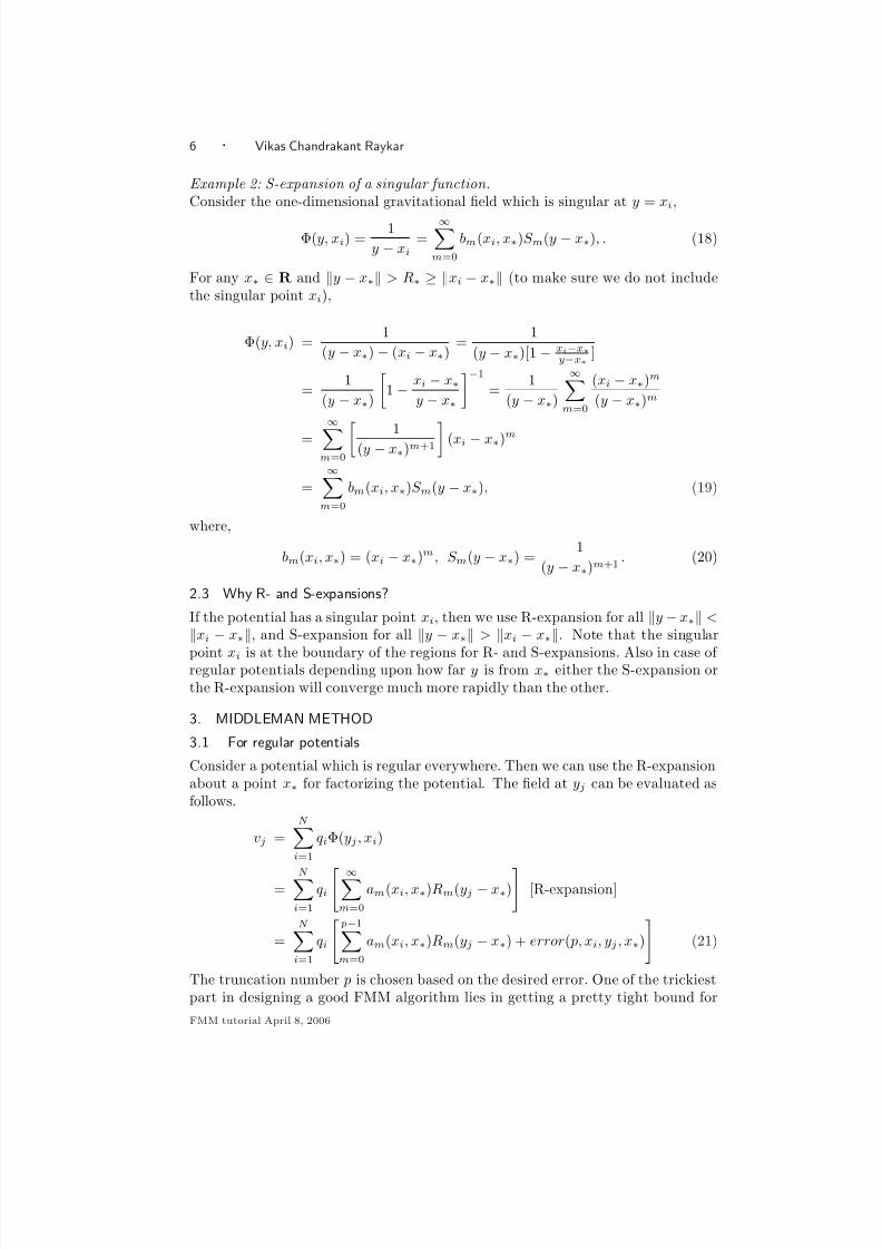
Fig. 3. (a) Direct computation (b) Middleman method (c) middleman with target clusters (d)middleman with source clusters (e) Single level FMM.

error( p, xi, yj, x∗). Ignoring the error term we have,

vj =N i=1

qi

p−1m=0

am(xi, x∗)Rm(yj − x∗)

=

p−1m=0

N i=1

qiam(xi, x∗)

Rm(yj − x∗)

=

p−1m=0

AmRm(yj − x∗) (22)

where Am = N i=1 qiam(xi, x∗), which depends only on the source and can be com-

puted in one pass for different m. The computational complexity for computingAm p−1

m=0 if O( pN ) and for computing vjM j=1 is O( pM ). Hence the total compu-

tational cost is O( pN + pM ). As long as p min(M, N ) we have a reduction inthe computational complexity.

This approach is called the middleman method since we are computing the set of coefficients Am p−1

m=0 at a single expansion center x∗ (see Fig. 3(b)). The readershould realize that this approach will work only for regular potentials. Also it canbe seen that the middleman method need not use only one expansion center. Wecan use multiple expansion centers and them consolidate the contribution of all theexpansion centers (see Fig. 3(c)).

3.2 For singular potentials

For singular potentials we can use the middleman approach if the source and thetarget points are well separated. [See Fig. 4(a) and (b)]. In (a) and (b) we will usethe R-expansion at the center of each target clusters and in (d) and (e) we will usethe S-expansion at the center of each source clusters.

If the sources and targets are not well separated we do a space partitioning. Forexample let us say we partition with respect to the target points. For each targetcluster we use the R-expansion for all sources outside a neighborhood of the cluster.There will be some sources which happen to lie within the neighborhood of these





x∗

r∗

1

(a)

1

(b)

1

(c)

x∗

R∗

1

(d)

1

(e)

1

(f)

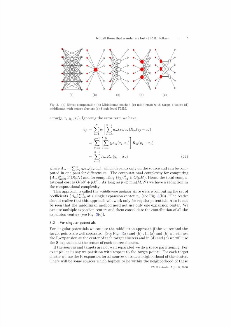
Fig. 4. For singular potentials we can use the middleman approach if the source and the targetpoints are well separated. In (a) and (b) we will use the R-expansion at the center of each targetclusters and in (d) and (e) we will use the S-expansion at the center of each source clusters. Thered filled circles are the source points and the back circles are the target points.

clusters, where the potential happens to be singular at each of these source points.If the number of such sources is few we can directly sum the contribution of thesesources. However if they are large in number, this leads to the idea of a single levelFMM to be discussed in the next section.

4. TRANSLATIONS (RE-EXPANSIONS)

Let F n(y −x∗1)∞n=0 and Gm(y −x∗2)∞m=0 be two sets of basis functions centeredat x∗1 and x∗1 such that Φ(y, xi) can be represented by two uniformly and absolutelyconvergent series as,

Φ(y, xi) =

∞

n=0

an(xi, x∗1)F n(y − x∗1), ∀y ∈ Ω1 ⊂ Rd. (23)

Φ(y, xi) =

∞m=0

bm(xi, x∗2)Gm(y − x∗2), ∀y ∈ Ω2 ⊂ Ω1. (24)

(F |G)(t) is called a translation operator which relates the two sets of coefficientsas,

bm(xi, x∗2) = (F |G)(t)an(xi, x∗1), t = x∗2 − x∗1. (25)





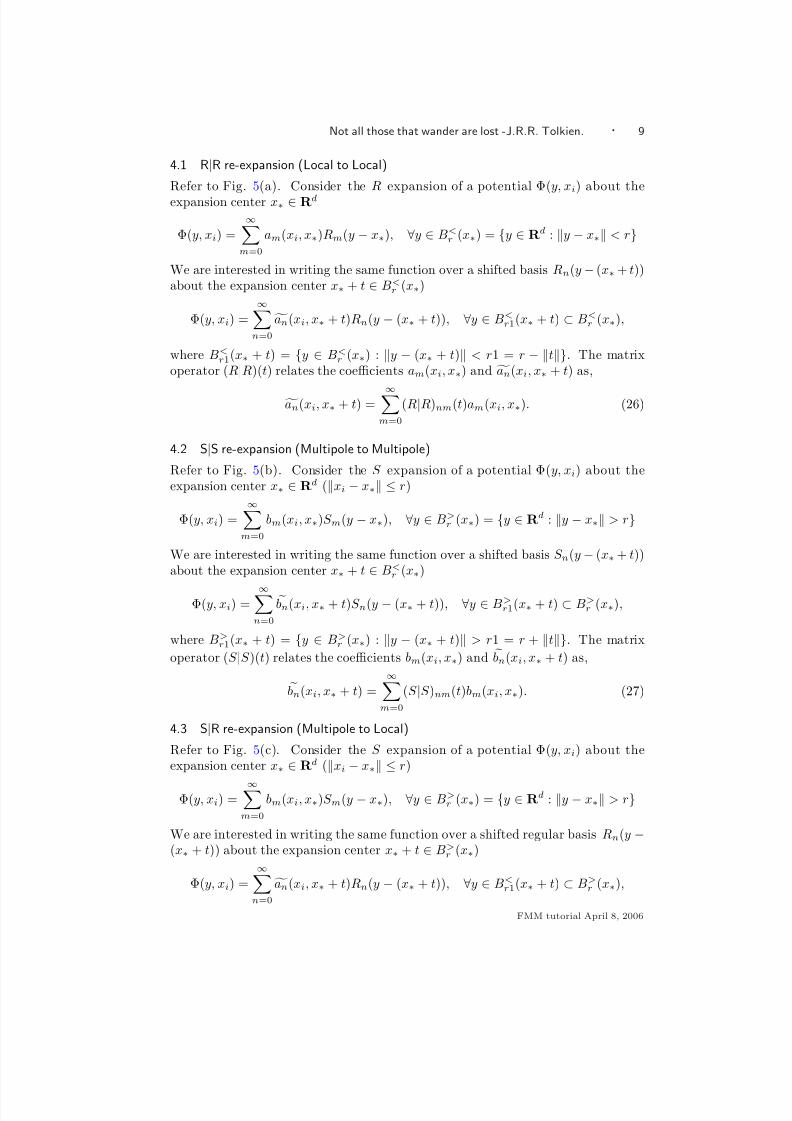
4.1 R|R re-expansion (Local to Local)

Refer to Fig. 5(a). Consider the R expansion of a potential Φ(y, xi) about theexpansion center x∗ ∈ Rd

Φ(y, xi) =

∞m=0

am(xi, x∗)Rm(y − x∗), ∀y ∈ B<r (x∗) = y ∈ Rd : y − x∗ < r

We are interested in writing the same function over a shifted basis Rn(y − (x∗ + t))about the expansion center x∗ + t ∈ B<

r (x∗)

Φ(y, xi) =

∞n=0

an(xi, x∗ + t)Rn(y − (x∗ + t)), ∀y ∈ B<r1(x∗ + t) ⊂ B<

r (x∗),

where B<r1(x∗ + t) = y ∈ B<

r (x∗) : y − (x∗ + t) < r1 = r − t. The matrixoperator (R|R)(t) relates the coefficients am(xi, x∗) and

an(xi, x∗ + t) as,

an(xi, x∗ + t) =∞

m=0

(R|R)nm(t)am(xi, x∗). (26)

4.2 S|S re-expansion (Multipole to Multipole)

Refer to Fig. 5(b). Consider the S expansion of a potential Φ(y, xi) about theexpansion center x∗ ∈ Rd (xi − x∗ ≤ r)

Φ(y, xi) =

∞m=0

bm(xi, x∗)S m(y − x∗), ∀y ∈ B>r (x∗) = y ∈ Rd : y − x∗ > r

We are interested in writing the same function over a shifted basis S n(y − (x∗ + t))about the expansion center x∗ + t ∈ B<

r (x∗)

Φ(y, xi) =∞n=0

bn(xi, x∗ + t)S n(y − (x∗ + t)), ∀y ∈ B>r1(x∗ + t) ⊂ B>

r (x∗),

where B>r1(x∗ + t) = y ∈ B>

r (x∗) : y − (x∗ + t) > r1 = r + t. The matrix

operator (S |S )(t) relates the coefficients bm(xi, x∗) and bn(xi, x∗ + t) as,

bn(xi, x∗ + t) =

∞m=0

(S |S )nm(t)bm(xi, x∗). (27)

4.3 S|R re-expansion (Multipole to Local)

Refer to Fig. 5(c). Consider the S expansion of a potential Φ(y, xi) about theexpansion center x∗ ∈ Rd (xi − x∗ ≤ r)

Φ(y, xi) =∞

m=0

bm(xi, x∗)S m(y − x∗), ∀y ∈ B>r (x∗) = y ∈ Rd : y − x∗ > r

We are interested in writing the same function over a shifted regular basis Rn(y −(x∗ + t)) about the expansion center x∗ + t ∈ B>

r (x∗)

Φ(y, xi) =∞n=0

an(xi, x∗ + t)Rn(y − (x∗ + t)), ∀y ∈ B<r1(x∗ + t) ⊂ B>

r (x∗),





x∗

x∗ + t

r

r1

t

y

B<

r(x∗)

B<

r1(x∗ + t)

1

(a) R|R

x∗ + t

x∗ r1

r

B>r1(x∗ + t)

B>r (x∗)

y

t

xi

1

(b) S|S

x∗

x∗ + t

r

r1

t

y

xi

B>r (x∗)

B<r1(x∗ + t)

1

(c) S|R

Fig. 5. Schematic illustrating (a) R|R re-expansion, (b) S|S re-expansion, and (c) S|R re-expansion

where B<r1(x∗ + t) = y ∈ B>

r (x∗) : y − (x∗ + t) < r1 = t − r. The matrixoperator (S |R)(t) relates the coefficients bm(xi, x∗) and

an(xi, x∗ + t) as,

an(xi, x∗ + t) =

∞

m=0

(S |R)nm(t)bm(xi, x∗). (28)

4.4 R|S re-expansion (Local to Multipole)

Theoretically it is possible to have R|S re-expansion also. But in practice since thedomain of S expansion is larger than the domain of R expansion, this is either notuseful (due to large error bounds) or can be avoided in algorithms. Most FMMalgorithms do not use R|S re-expansion.





1

(a) I 1(n)

1

(b) I 2(n)

1

(c) I 3(n)

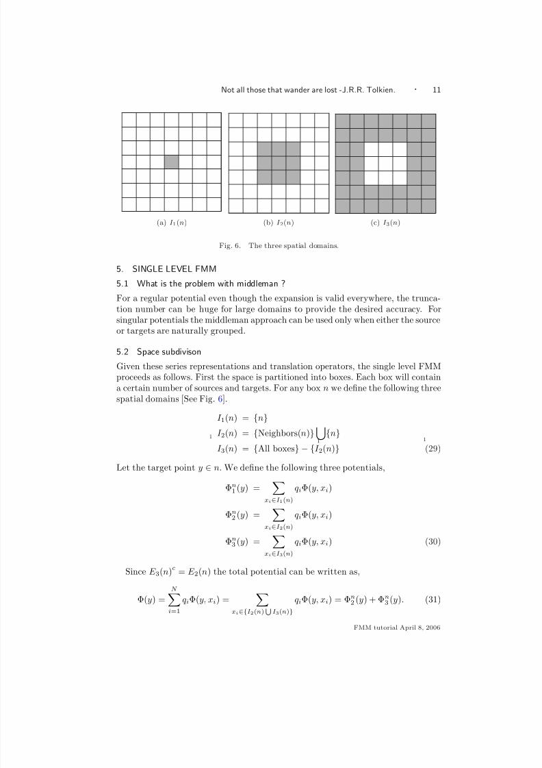
Fig. 6. The three spatial domains.

5. SINGLE LEVEL FMM5.1 What is the problem with middleman ?

For a regular potential even though the expansion is valid everywhere, the trunca-tion number can be huge for large domains to provide the desired accuracy. Forsingular potentials the middleman approach can be used only when either the sourceor targets are naturally grouped.

5.2 Space subdivison

Given these series representations and translation operators, the single level FMMproceeds as follows. First the space is partitioned into boxes. Each box will containa certain number of sources and targets. For any box n we define the following three

spatial domains [See Fig. 6].I 1(n) = n

I 2(n) = Neighbors(n)

n

I 3(n) = All boxes − I 2(n) (29)

Let the target point y ∈ n. We define the following three potentials,

Φn1 (y) =

xi∈I 1(n)

qiΦ(y, xi)

Φn2 (y) =

xi∈I 2(n)

qiΦ(y, xi)

Φn3 (y) =

xi∈I 3(n)

qiΦ(y, xi) (30)

Since E 3(n)c

= E 2(n) the total potential can be written as,

Φ(y) =N i=1

qiΦ(y, xi) =

xi∈I 2(n)I 3(n)

qiΦ(y, xi) = Φn2 (y) + Φn

3 (y). (31)





5.3 R expansion

The potential Φn

3

(y) has to be computed using the local R expansion of Φ( y, xi)about the box center xn

c . Exchanging the order of summation and consolidatingthe source terms we have,

Φn3 (y) =

xi∈I 3(n)

qiΦ(y, xi)

=

xi∈I 3(n)

qi

∞

m=0

am(xi, xnc )Rm(y − xnc )

=

∞m=0

xi∈I 3(n)

qiam(xi, xnc )

Rm(y − xnc )

=∞

m=0

AnmRm(y − xnc ) (32)

where Anm =

xi∈I 3(n) qiam(xi, xnc ).

5.4 S expansion

If y is close to xnc then the local R-expansion series will converge quickly. Howeverif y is faraway then the series may converge very slowly or may nor converge at all.We need a larger radius of convergence so that the number of boxes are small. Alsosince we will be truncating the above series, if the series converges slowly larger

radius will imply a very large truncation number. For this reason we use the S-expansions, and translate it to an R-expansion via the S|R translation operator. TheS expansions are computed about the box centers for all the boxes. Exchanging theorder of summation and consolidating the source terms we have Φl

1(y) the potentialat y ∈ I 3(l) due to all sources xi ∈ I 1(l)

Φl1(y) =

xi∈I 1(l)

qiΦ(y, xi)

=

xi∈I 1(l)

qi

∞

m=0

bm(xi, xlc)S m(y − xlc)

=

∞m=0

xi∈I 1(l)

qibm(xi, xlc)S m(y − xlc)

=

∞m=0

BlmS m(y − xlc) (33)

where Blm =

xi∈I 1(l) qibm(xi, xlc).





5.5 S|R Translation

Now we want to write the potential Φl1(y) (expanded using an S expansion around

xlc) as an R expansion around xnc .

Φl1(y) =

xi∈I 1(l)

qi

∞

m=0

bm(xi, xlc)S m(y − xlc)

=

xi∈I 1(n)

qi

∞k=0

ak xi, xlc + (xnc − xlc)

Rk

y −

xlc + (xnc − xl

c)

=

∞k=0

xi∈I 1(l)

qiak xi, xlc + (xnc − xlc)Rk(y − xnc )

=

∞k=0

xi∈I 1(l)

qi ∞m=0

(S |R)km(xnc − x

lc)bm(xi, x

lc)Rk(y − x

nc )

=

∞k=0

∞m=0

(S |R)km(xnc − xlc)

xi∈I 1(l)

qibm(xi, xlc)

Rk(y − xnc )

=∞k=0

∞

m=0

(S |R)km(xnc − xlc)Blm

Rk(y − xnc )

=

∞k=0

Anlk Rk(y − xnc ) (34)

where Anlk = ∞

m=0(S |R)km(xnc − xlc)Blm. The R expansions about the box center

xnc ,

Φn3 (y) =

∞m=0

AnmRm(y − xnc ) (35)

where Anm =

xi∈I 3(n) qiam(xi, xnc ) =

l∈I 3(n)

Anlm . So we have R expansions

about the box centers, and very few points for which valid expansions could not beconstructed. These are evaluated directly and added to the R expansions evaluatedat the evaluation points. The speedup is achieved by appropriately truncating eachseries.

6. MULTI LEVEL FMM

We give a brief description of the multi level FMM without going into the details.Given these series representations and translation operators, the multilevel FMMproceeds as follows. First the space is partitioned into boxes at various levels,and outer S expansions computed about box centers at the finest level, for pointswithin the box. These expansions are consolidated, and they are translated S|Susing translations in an upward pass up the hierarchy. The coefficients of these box-centered expansions at each level are stored. In the downward pass, the consolidatedS expansions are expanded as local R expansions about boxes in the evaluation





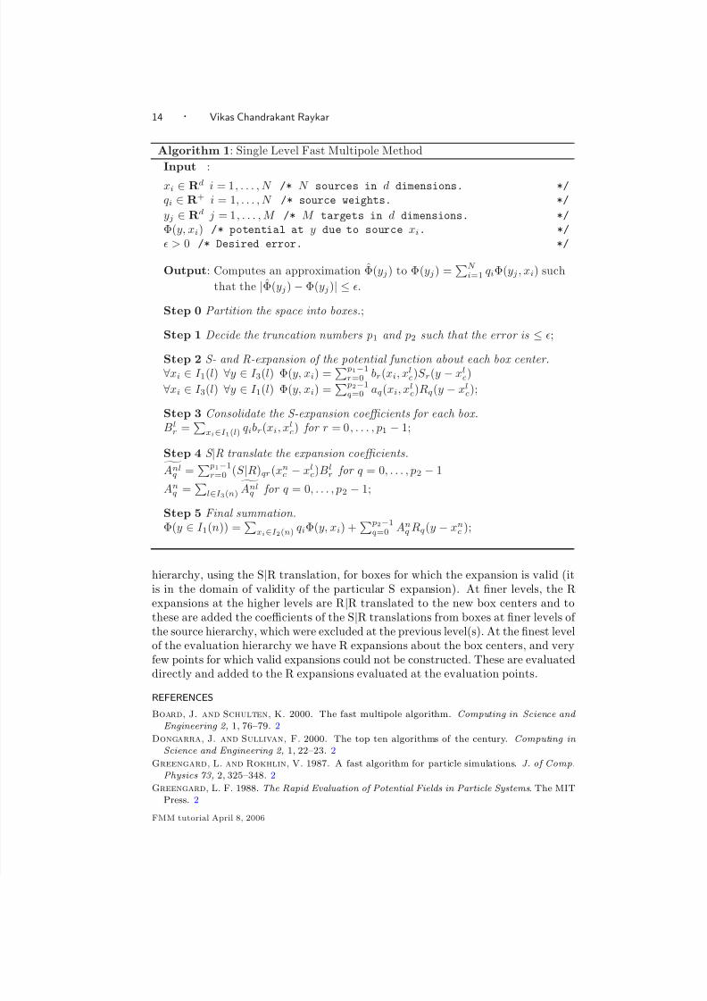
Algorithm 1: Single Level Fast Multipole Method

Input :

xi ∈ Rd i = 1, . . . , N /* N sources in d dimensions. */

qi ∈ R+ i = 1, . . . , N /* source weights. */

yj ∈ Rd j = 1, . . . , M /* M targets in d dimensions. */

Φ(y, xi) /* potential at y due to source xi. */

> 0 /* Desired error. */

Output: Computes an approximation Φ(yj) to Φ(yj) =N

i=1 qiΦ(yj , xi) such

that the |Φ(yj) − Φ(yj)| ≤ .

Step 0 Partition the space into boxes.;

Step 1 Decide the truncation numbers p1 and p2 such that the error is ≤ ;

Step 2 S- and R-expansion of the potential function about each box center.∀xi ∈ I 1(l) ∀y ∈ I 3(l) Φ(y, xi) =

p1−1r=0 br(xi, xlc)S r(y − xl

c)

∀xi ∈ I 3(l) ∀y ∈ I 1(l) Φ(y, xi) = p2−1

q=0 aq(xi, xlc)Rq(y − xlc);

Step 3 Consolidate the S-expansion coefficients for each box.Blr =

xi∈I 1(l) qibr(xi, xlc) for r = 0, . . . , p1 − 1;

Step 4 S |R translate the expansion coefficients.Anlq =

p1−1r=0 (S |R)qr(xnc − xlc)Bl

r for q = 0, . . . , p2 − 1

Anq =

l∈I 3(n)

Anlq for q = 0, . . . , p2 − 1;

Step 5 Final summation.

Φ(y ∈ I 1(n)) = xi∈I 2(n) qiΦ(y, xi) + p2−1q=0 Anq Rq(y − xnc );

hierarchy, using the S|R translation, for boxes for which the expansion is valid (itis in the domain of validity of the particular S expansion). At finer levels, the Rexpansions at the higher levels are R|R translated to the new box centers and tothese are added the coefficients of the S|R translations from boxes at finer levels of the source hierarchy, which were excluded at the previous level(s). At the finest levelof the evaluation hierarchy we have R expansions about the box centers, and veryfew points for which valid expansions could not be constructed. These are evaluateddirectly and added to the R expansions evaluated at the evaluation points.

REFERENCES

Board, J. and Schulten, K. 2000. The fast multipole algorithm. Computing in Science and

Engineering 2, 1, 76–79. 2

Dongarra, J. and Sullivan, F. 2000. The top ten algorithms of the century. Computing in

Science and Engineering 2, 1, 22–23. 2

Greengard, L. and Rokhlin, V. 1987. A fast algorithm for particle simulations. J. of Comp.

Physics 73, 2, 325–348. 2

Greengard, L. F. 1988. The Rapid Evaluation of Potential Fields in Particle Systems. The MITPress. 2


fmm tutorial

Documents