focus on geology to define subsurface migration … sequence stratigraphy (essenvironmental sequence...
TRANSCRIPT
Focus on Geology to Define Subsurface Migration Pathways
Rick Cramer, MS, PG (Orange, CA) Mik Sh lt PhD (C d CA)Mike Shultz, PhD (Concord, CA)
December 2, 2015

OutlineOutline
Introduction
Why does geology matter?
What is Environmental Sequence Stratigraphy?
Proof of conceptProof of concept The technology
Case Studies
Page 2
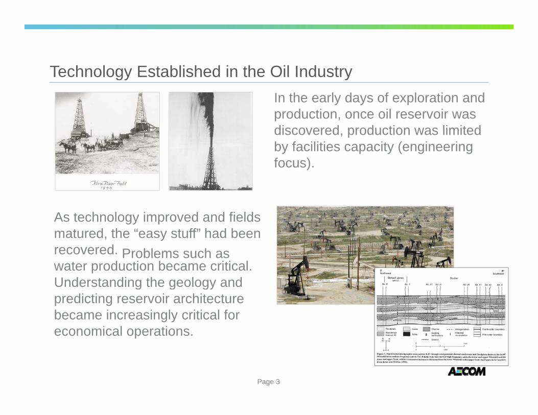
Technology Established in the Oil IndustryTechnology Established in the Oil Industry
In the early days of exploration and production, once oil reservoir was discovered production was limited discovered, production was limited by facilities capacity (engineering focus).
As technology improved and fields matured the “easy stuff” had been had beenmatured, the easy stuff recovered. Problems such as water production became critical. Understanding the geology andUnderstanding the geology and predicting reservoir architecture became increasingly critical for economical operations.
Page 3
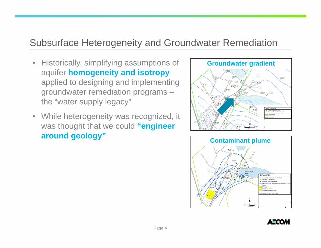
Subsurface Heterogeneity and Groundwater RemediationSubsurface Heterogeneity and Groundwater Remediation
• Historically, simplifying assumptions ofaquifer homogeneity and isotropyapplied to designing and implementinggroundwater remediation programs –the “water supply legacy”
• While heterogeneity was recognized, itwas thought that we could “engineeraround ggeology”gy Contaminant plume
Groundwater gradient
Contaminant plume
Page 4
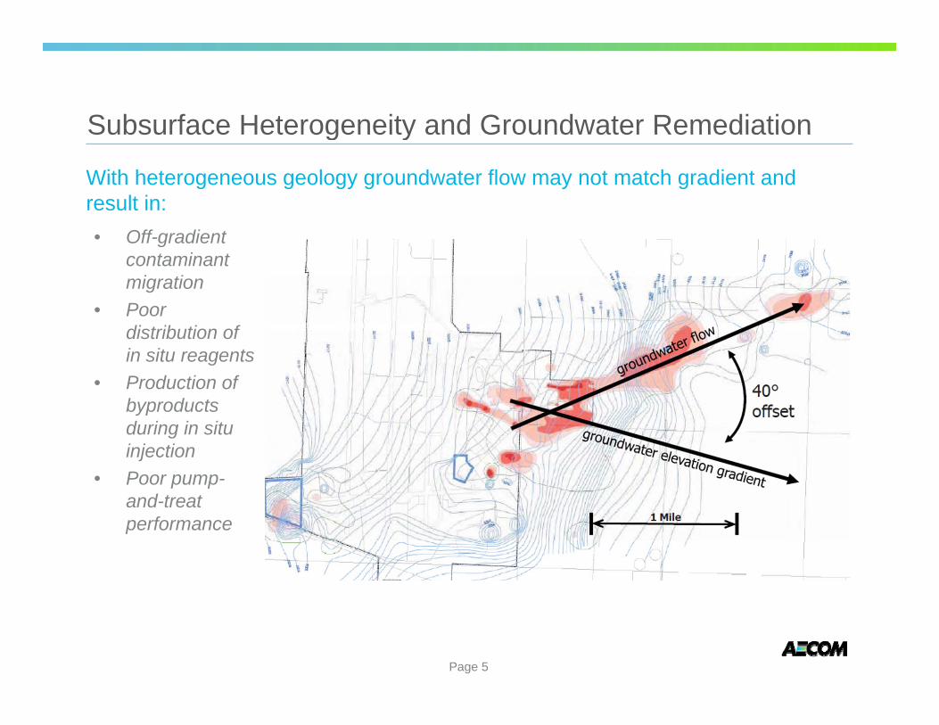
Subsurface Heterogeneity and Groundwater RemediationSubsurface Heterogeneity and Groundwater Remediation
With heterogeneous geology groundwater flow may not match gradient and result in: • Off-gradient
contaminantmigration
• Poordistribution ofin situ reagents
• Production ofbyproductsbyproductsduring in situinjection
• Poor pump-andand-treattreatperformance
Page 5
Why Geology MattersWhy Geology Matters
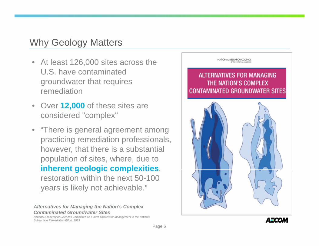
• At least 126,000 sites across theU.S. have contaminatedgroundwater that requiresremediation
• Over 12,000 of these sites areOver 12,000 of these sites areconsidered "complex"
• “There is general agreement amongpracticing remediation professionalspracticing remediation professionals,however, that there is a substantialpopulation of sites, where, due toinherent geologic complexitiesinherent geologic complexities,restoration within the next 50-100years is likely not achievable.”
Alternatives for Managing the Nation's Complex Contaminated Groundwater Sites National Academy of Sciences Committee on Future Options for Management in the Nation's Subsurface Remediation Effort, 2013
Page 6
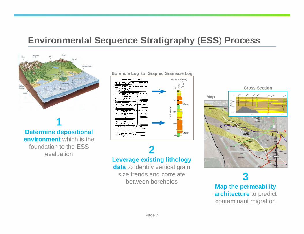
Environmental Sequence Stratigraphy (ESS) ProcessEnvironmental Sequence Stratigraphy (ESS) Process
Borehole Log Borehole Log toto Graphic Grainsize Log Graphic Grainsize Log Grain-size increasing
Clay
Grav
el
0 Cross Section
Map100
Uncon
200
Dept
h (Ft
- MSL
)
1 300
Determine depositionalDetermine depositional environment which is the
foundation to the ESS evaluation
Uncon
400
2 Leverage existing lithology Leverage existing lithology data to identify vertical grain
size trends and correlate between boreholes 3
Map the permeability architecture to predict contaminant migration
Page 7
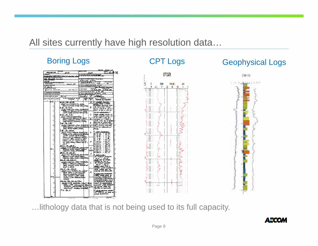
All sites currently have high resolution data…All sites currently have high resolution data…
Boring Logs CPT Logs Geophysical Logs
…lithology data that is not being used to its full capacity.
Page 8
Environmental Sequence Stratigraphy (ESS)Environmental Sequence Stratigraphy (ESS)
Beauty of this approach is that the data are l d id f d th Oil I d t halready paid for and the Oil Industry has
already invested billions in developing the t h ltechnology.
Page 9
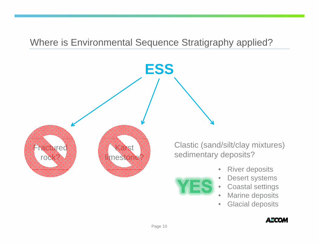
Where is Environmental Sequence Stratigraphy applied?Where is Environmental Sequence Stratigraphy applied?
ESS
Fractured rock?
Karst limestone?
Clastic (sand/silt/clay mixtures) sedimentary deposits?
•• River deposits River deposits • Desert systems• Coastal settings• Marine deposits• Glacial deposits
Page 10
Focus on geology improves site characterization throughout the remediation life cycle:the remediation life cycle:
• Data gaps investigations, high-resolution site characterizationprograms
• Optimizing groundwater monitoring programs
• Contaminant source identification for comingled plumes
• Mass flux/mass discharge analysis (contaminant transport vscontaminant storage zones)
•• In situ remediation (optimize distribution)In situ remediation (optimize distribution)
• Optimizing pump and treat programs
• Alternative endpoint analysisAlternative endpoint analysis
Page 11
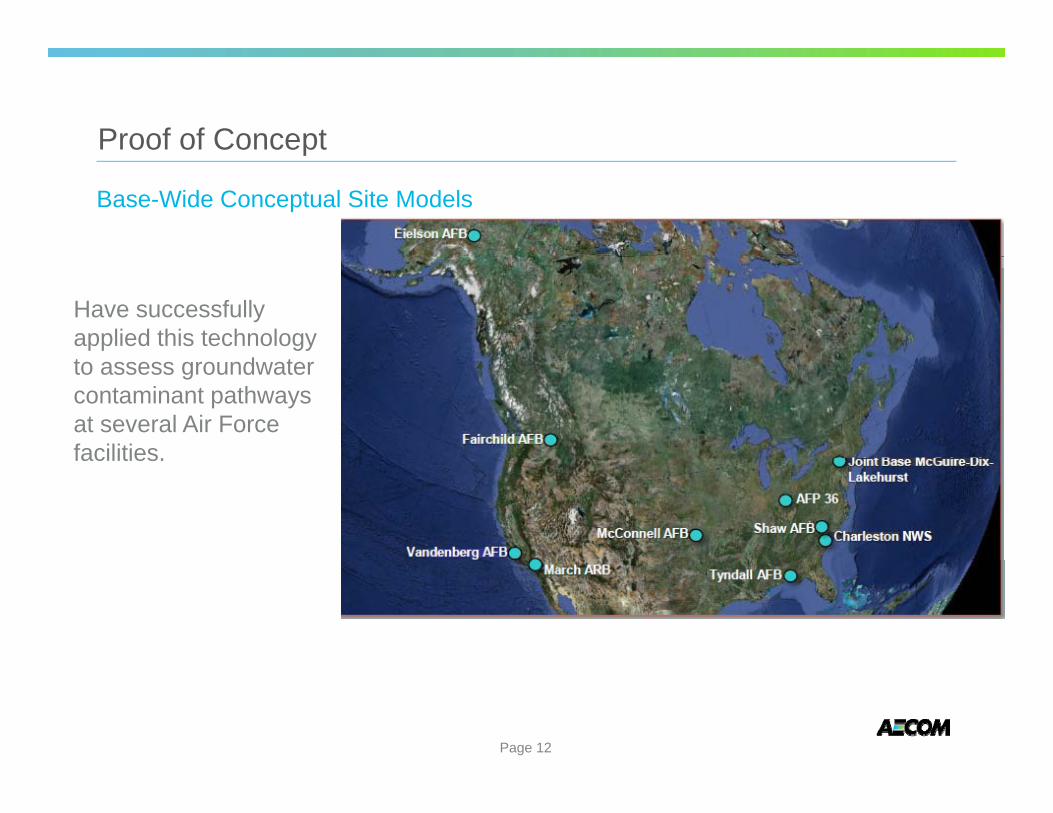
Proof of Conceppt
Have successfully applied this technology to assess groundwater contaminant pathways at several Air Force facilitiesfacilities.
Base-Wide Conceptual Site Models
Page 12
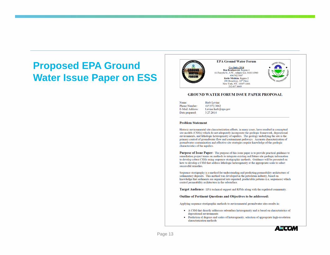
Proposed EPA Ground Water Issue Paper on ESSWater Issue Paper on ESS
Page 13
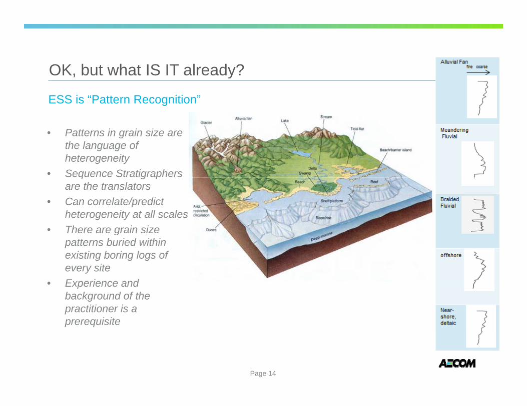
OK, but what IS IT already?OK, but what IS IT already?
ESS is “Pattern Recognition”
• Patterns in grain size arethe language ofheterogeneity
• Seqquence Stratigg praphersare the translators
• Can correlate/predictheterogeneity at all scales
•• There are grain sizeThere are grain sizepatterns buried withinexisting boring logs ofevery site
• EExperiience anddbackground of thepractitioner is aprerequisite
Page 14
A lluvial Fan ... "'""
7 Meandering Fluv ial
) Braided
~ Fluvial
offshore
) Near-
7 shore, deltaic
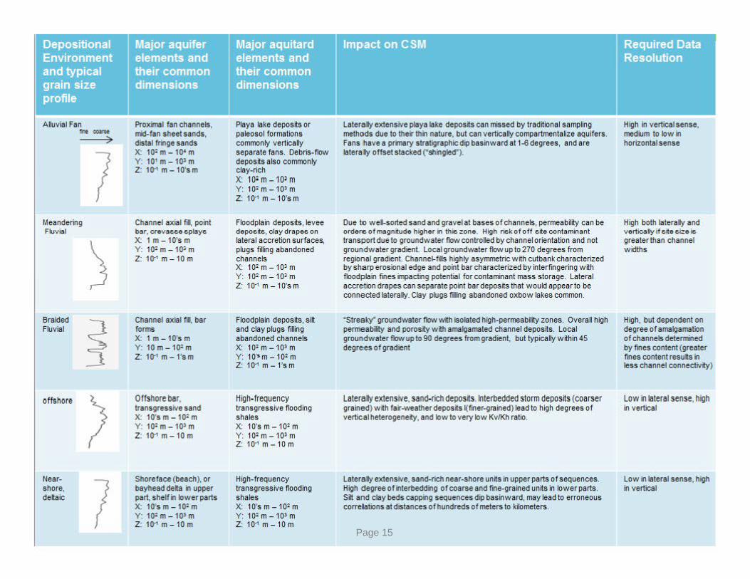
Proximal fan channels, mid-fan sheet sands , distal fringe sands X: 102 m - 10' m Y : 101 m - 1 0~ m Z: 10"1 m - 11Ysm
Channel ax ial fill, point bar, c revaeee e-playeX:1 m - 11Ys m Y: 10' m- 10' m Z:10"1 m - 10 m
Channel ax ial fill, bar forms X:1 m - 11Ys m Y : 10 m - 102 m Z: 10"1 m - 1's m
Offshore bar, transgressive sand X: 11Ys m - 102 m Y: 10' m- 10' m Z:10"1 m - 10 m
Shoreface (beach}, or bayhead delta in upper part, shelf in low er parts X: 10's m - 10' m Y: 102 m - 1 0~ m Z: 10"1 m - 10 m
Playa lake deposHs or paleosol formations commonly vertically separate fans. Debris-flow deposHs also commonly clay-rich X: 10' m - 10' m Y : 10' m - 10' m Z: 10"1 m - 11Ysm
Floodplain deposHs, levee depoe-ite, c lay drapee- on lateral accretion surfac~
plugs filling abandoned channels X: 10' m- 10' m Y: 10' m- 10' m Z: 10"1 m - 11Ysm
Floodplain deposHs, silt and clay plugs filling abandoned channels X: 10' m - 10' m Y : 1o·s m - 102 m Z: 10"1 m - 1's m
High-frequency transgressive flooding shales X: 11Ys m - 102 m Y: 10' m- 10' m Z:10"1 m - 10 m
High-frequency transgressive flooding shales X: 10's m - 10' m Y: 102 m - 1 0~ m Z: 10"1 m - 10 m
Laterally extensive playa lake deposHs can missed by tradHional sampling methods due to their thin nature, but can vertically compartmentalize aquifers. Fans have a primary stratigraphic dip basin w ard at 1-6 degrees, and are laterally offset slacked (' shingled").
Due to w ell-sorted sand and gravel at bases of channels, permeability can be ordere o f magnitude higher in thie zone. High riek of off e-ite contaminant transport due to groundw ater flow controlled by channel orientation and not groundw ater gradient. Local groundwater flow up to 270 degrees from regional gradient. Channel-fills highly asymmetric w Hh cutbank characterized by sharp erosional edge and point bar characterized by interfingering w Hh floodplain fines impacting potential for contaminant mass storage. Lateral accretion drapes can separate point bar deposHs that w ould appear to be connected laterally. Clay plugs filling abandoned oxbow lakes common.
"Strea~ groundwater flow wHh isolated high-permeability zones. Overall high permeability and porosity w Hh amalgamated channel deposHs. Local groundw ater flow up to 90 degrees from gradient, but typically w Hhin 45 degrees of gradient
Laterally extensive, sand-rich deposHs. lnterbedded storm deposHs (coarser grained} w Hh fair-weather deposHs l(finer-grained} lead to high degrees of vertic al heterogeneity, and low to very low Kv/Kh ratio.
Laterally extensive, sand-rich near-shore unHs in upper parts of sequences. High d egree of interbedding of coarse and fine-grained unHs in low er parts. Silt and clay beds capping sequences dip basinw ard, may lead to erroneous correlations at distances of hundreds of meters to kilometers.
High in vertical sense, medium to low in horizontal sense
High both laterally and vertically if e-ite e-ize ie greater than channel w idths
High, but dependent on degree of amalgamation of channels determined by fines content (greater fines content results in less channel connectivity}
Low in lateral sense, high in vertical
Low in lateral sense, high in vertical
Page 15
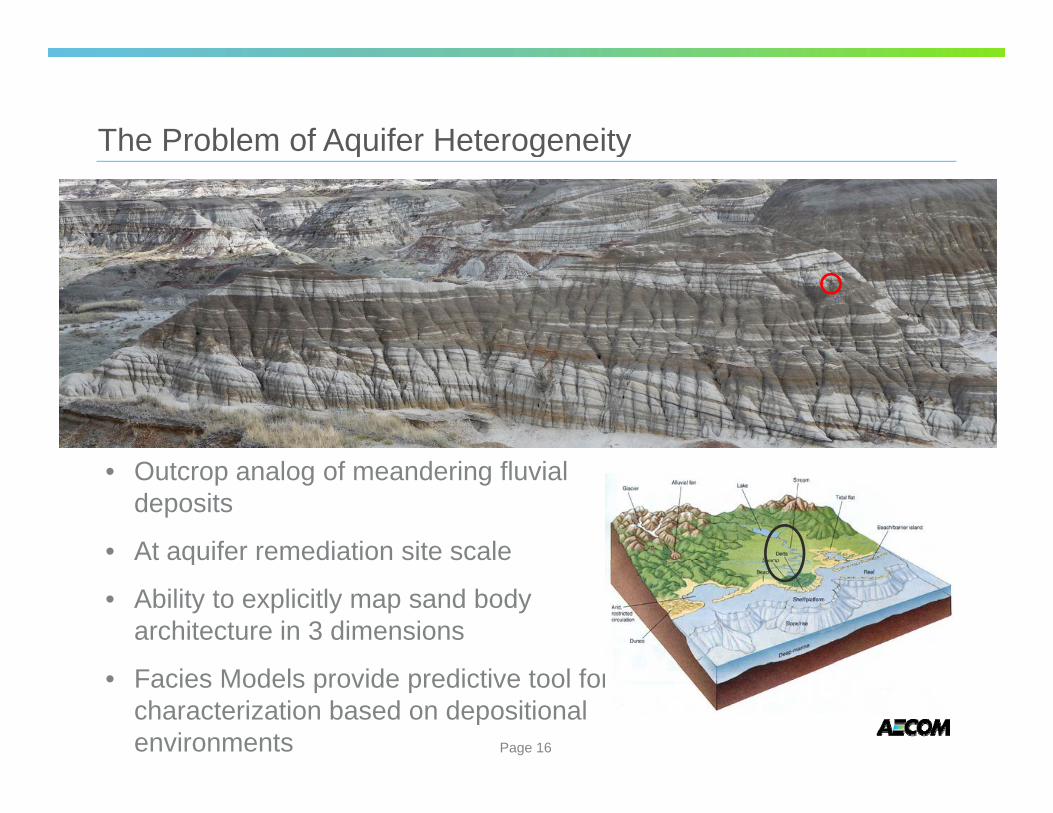
The Problem of Aquifer HeterogeneityThe Problem of Aquifer Heterogeneity
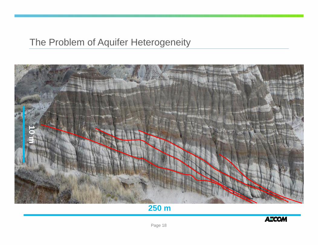
• Outcrop analog of meandering fluvialdeposits
• At aqquifer remediation site scale
• Ability to explicitly map sand bodyarchitecture in 3 dimensions
• Facies Models provide predictive tool forcharacterization based on depositionalenvironments Page 16
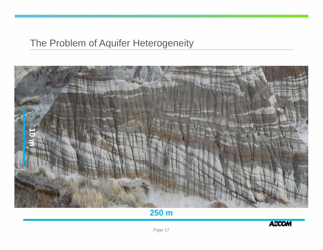
The Problem of Aquifer HeterogeneityThe Problem of Aquifer Heterogeneity
10 mm
250 m
Page 17
The Problem of Aquifer HeterogeneityThe Problem of Aquifer Heterogeneity
10 mm
250 m
Page 18
The Problem of Aquifer HeterogeneityThe Problem of Aquifer Heterogeneity
10 mm
250 m
Page 19
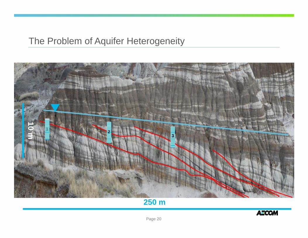
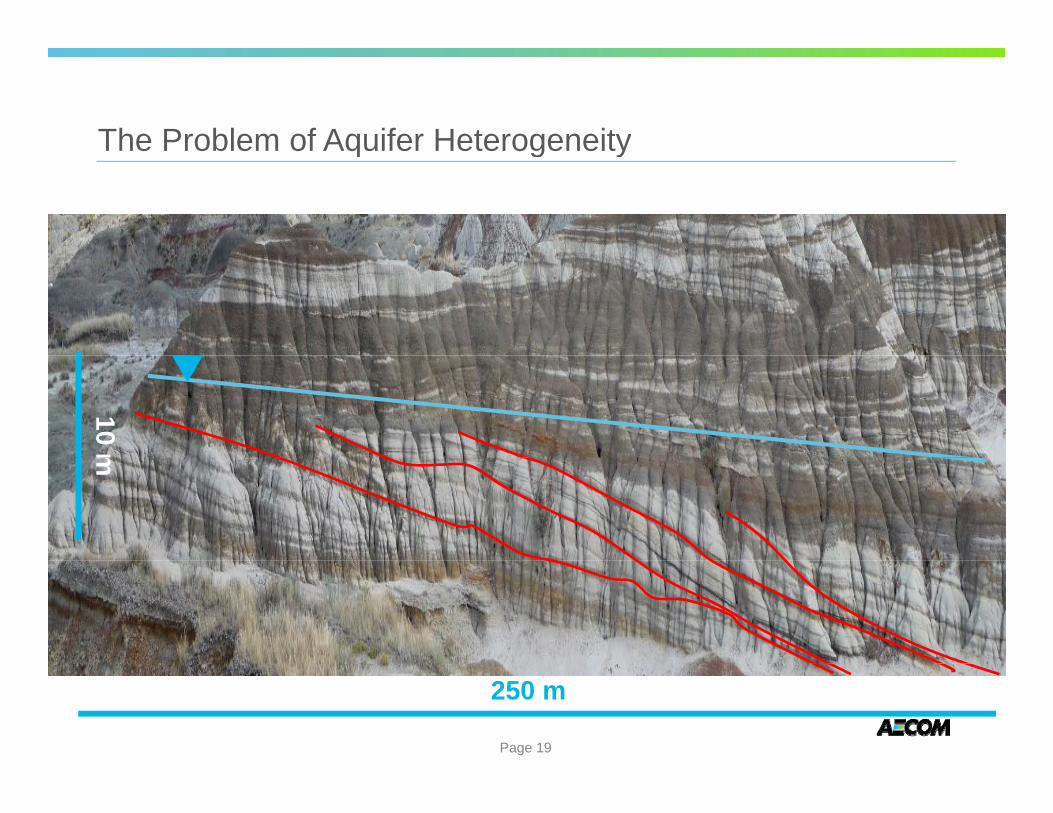
The Problem of Aquifer HeterogeneityThe Problem of Aquifer Heterogeneity
1 2
10 m
3
m
250 m
Page 20
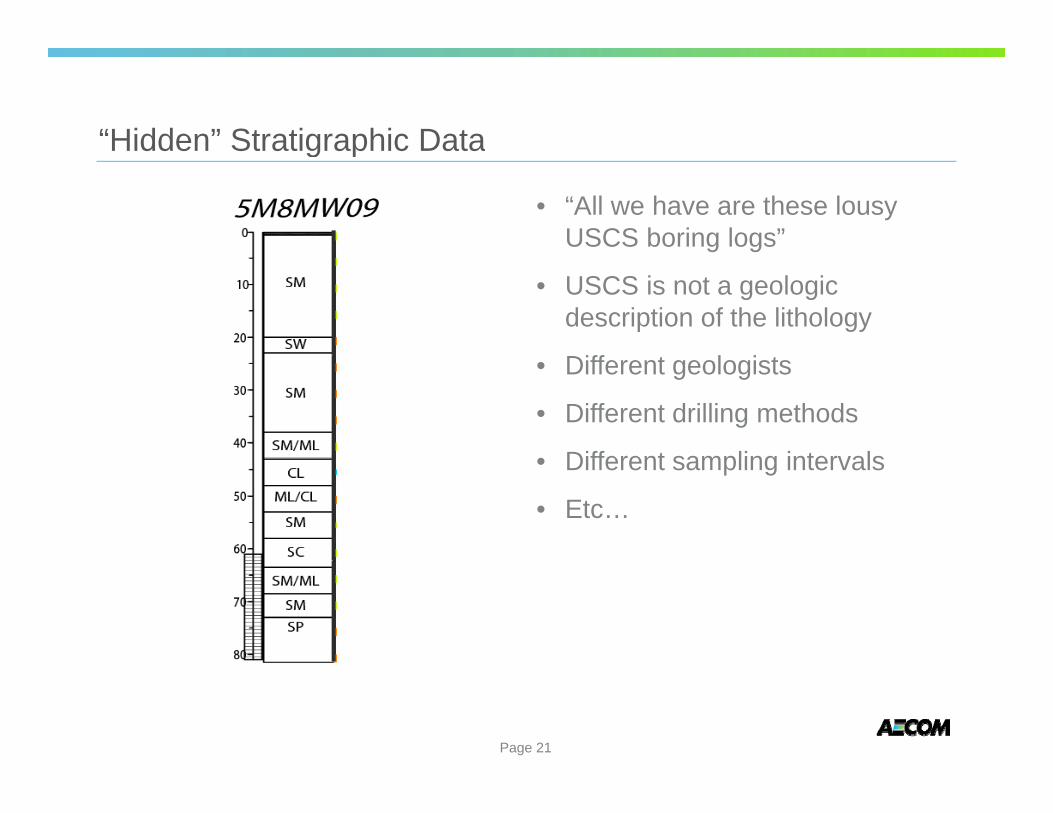
“Hidden” Stratigraphic Data Hidden Stratigraphic Data
• “All we have are these lousyUSCS boring logs”
• USCS is not a geologicdescription of the lithology
• Diff lDifferent geologiists
• Different drilling methods
•• Different sampling intervals Different sampling intervals
• Etc…
Page 21
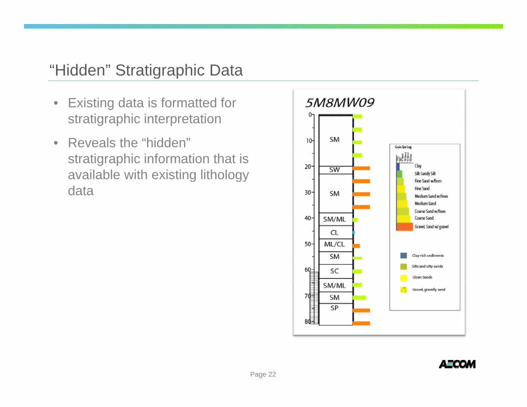
“Hidden” Stratigraphic Data Hidden Stratigraphic Data
• Existing data is formatted forstratigraphic interpretation
• Reveals the “hidden”stratigraphic information that isavailable with existing lithologyavailable with existing lithologydata
Page 22
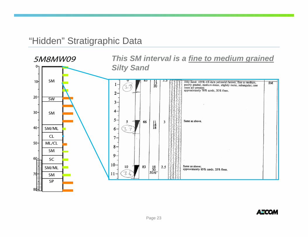
“Hidden” Stratigraphic Data Hidden Stratigraphic Data
This SM interval is a fine to medium grained Silty Sand
Page 23
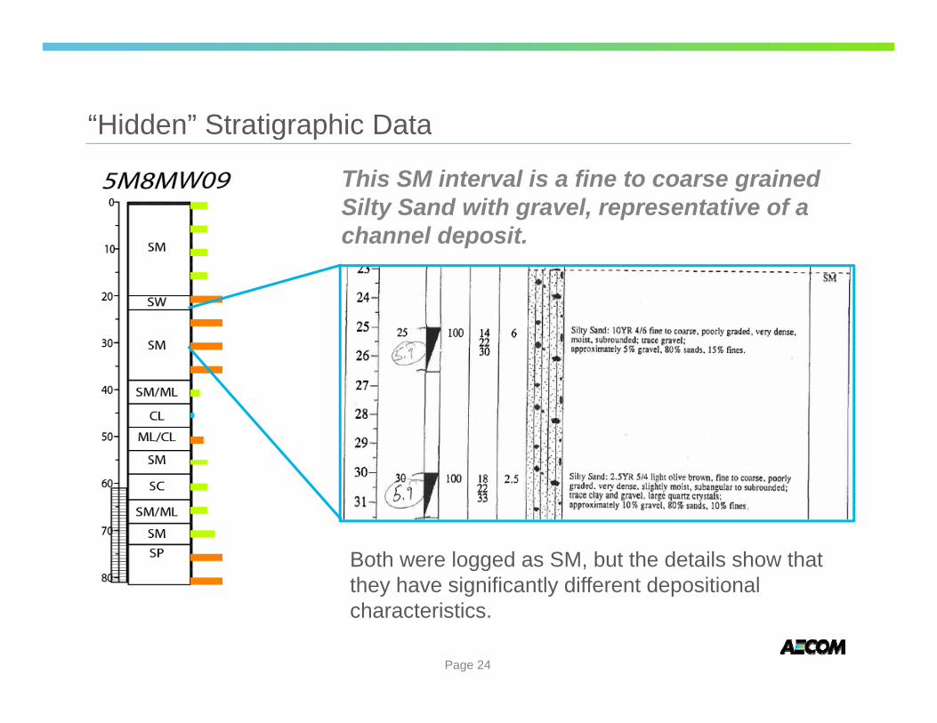
“Hidden” Stratigraphic Data Hidden Stratigraphic Data
This SM interval is a fine to coarse grained Silty Sand with gravel, representative of a channel deposit.
Both were logged as SM, but the details show that they have significantly different depositional they have significantly different depositional characteristics.
Page 24
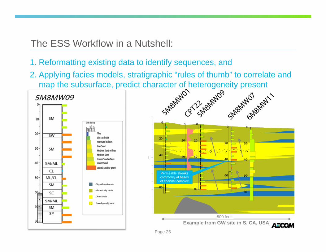
The ESS Workflow in a Nutshell:The ESS Workflow in a Nutshell:
1. Reformatting existing data to identify sequences, and2. Applying facies models, stratigraphic “rules of thumb” to correlate andpp y g , g p
map the subsurface, predict character of heterogeneity present
Fining-upward cycles indicative of channel-fillsPermeable streaksPermeable streaks
commonly at bases of channel complex
Page 25
Example from GW site in S. CA, USA 500 feet
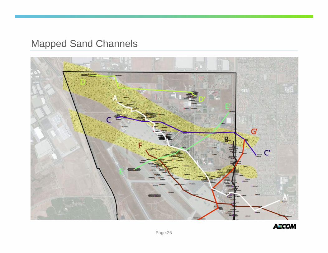
Mapped Sand ChannelsMapped Sand Channels
Page 26
Page 27
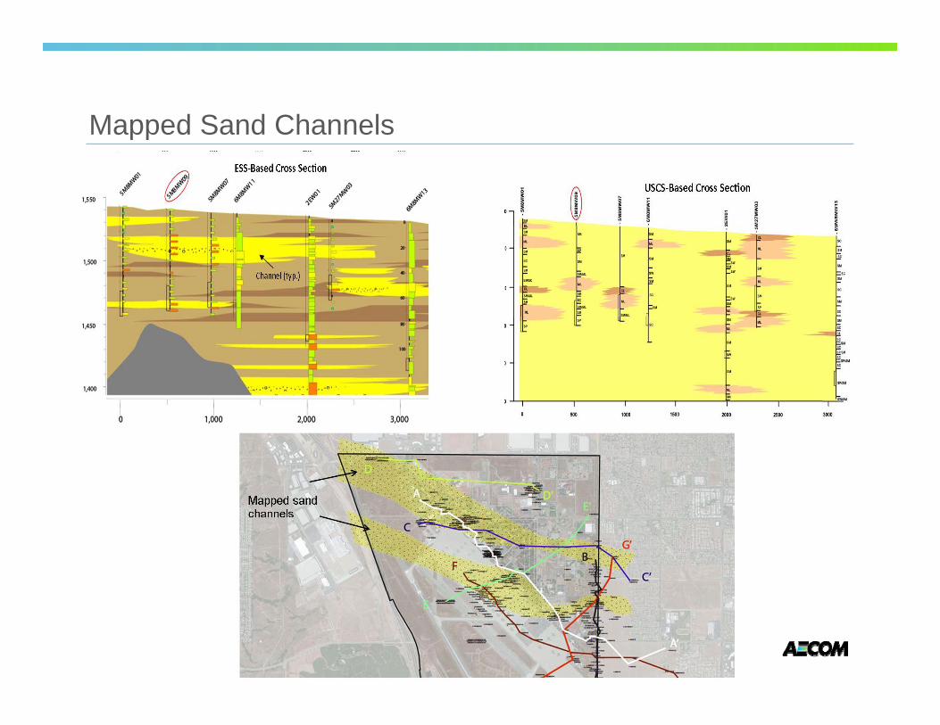
Mapped Sand ChannelsMapped Sand Channels
Case Study #1: In situ BioremediationCase Study #1: In situ Bioremediation
Industrial Facility: Ethanol injection to reduce hexavalent chromium plume
Scale: Hundred acres, ~60’ depth of investigation
Lithology Data: CPT logs, borehole logs
Approach: Apply ESS to explain Mn by-product
Takeaway: Even with “high-resolution” lithology data, a depositional model is needed for successful remediationmodel is needed for successful remediation
Page 28
C i d
Case Study #1: In situ Bioremediation
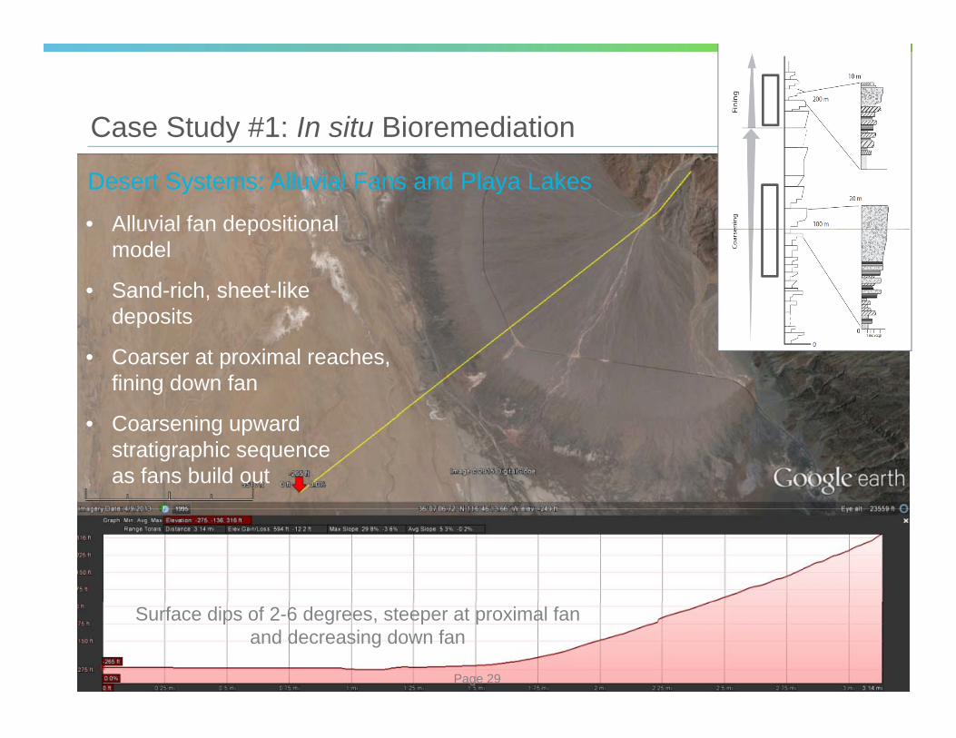
Desert Systems: Alluvial Fans and Playa Lakes
• Alluvial fan depositional
Case Study #1: In situ Bioremediation
Alluvial fan depositional model
• Sand-rich, sheet-likedepositsdeposits
• Coarser at proximal reaches,fining down fan
• Coarsening upwardstratigraphic sequenceas fans build out
Page 29
Surface dips of 2-6 degrees, steeper at proximal fan and decreasing down fan
Case Study #1: In situ BioremediationCase Study #1: In situ Bioremediation
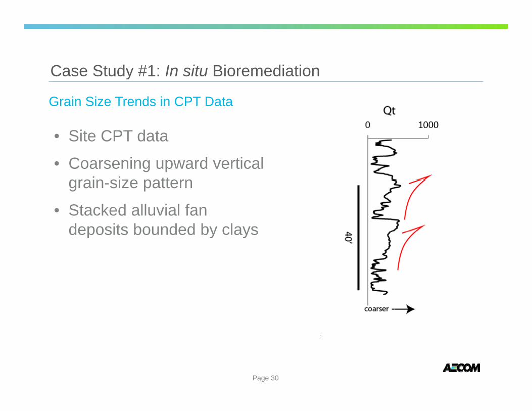
Grain Size Trends in CPT Data
• Site CPT data
• Coarsening upward verticalgrain si e pattern grain-size pattern
• Stacked alluvial fandeposits bounded by claysdeposits bounded by clays
Page 30
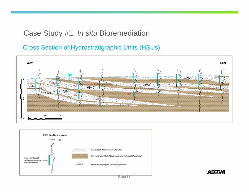
Case Study #1: In situ BioremediationCase Study #1: In situ Bioremediation
Cross Section of Hydrostratigraphic Units (HSUs)
Page 31
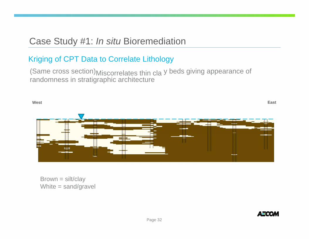
Case Study #1: In situ BioremediationCase Study #1: In situ Bioremediation
Kriging of CPT Data to Correlate Lithology ((Same cross section)) Miscorrelates thin cla yy beds ggivingg appearance ofpprandomness in stratigraphic architecture
West East
Brown = silt/clay White = sand/gravel
Page 32
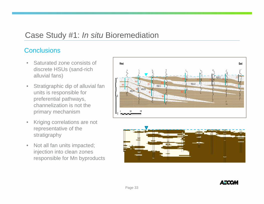
Case Study #1: In situ BioremediationCase Study #1: In situ Bioremediation
Conclusions
• Saturated zone consists ofSaturated zone consists ofdiscrete HSUs (sand-richalluvial fans)
• Stratigraphic dip of alluvial fanunits is responsible forpreferential pathways,channelization is not theprimary mechanism
• Kriging correlations are notrepresentative of thestratigraphy
• Not all fan units impacted;injection into clean zonesresponsible for Mn byproducts
Page 33
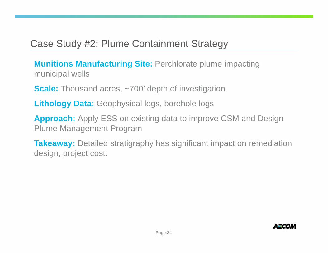
Case Study #2: Plume Containment StrategyCase Study #2: Plume Containment Strategy
Munitions Manufacturing Site: Perchlorate plume impacting municipal wells
Scale: Thousand acres, ~700’ depth of investigation
Lithology Data: Geophysical logs, borehole logs
Approach: Apply ESS on existing data to improve CSM and Design Plume Management Program
Takeaway:Takeaway: Detailed stratigraphy has significant impact on remediationDetailed stratigraphy has significant impact on remediation design, project cost.
Page 34
Case Study #2: Plume Containment Strategy Case Study #2: Plume Containment Strategy
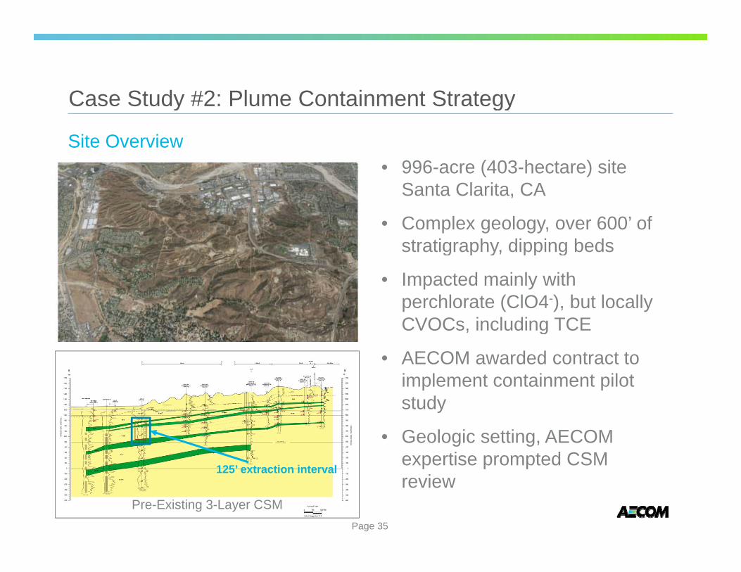
Site Overview
125’ t ti i t l125’ extraction interval
Pre-Existing 3-Layer CSM
• 996-acre (403-hectare) siteSanta Clarita, CA
• Complex geology, over 600’ ofstratigraphy, dipping bedsstratigraphy, dipping beds
• Impacted mainly withperchlorate (ClO4-), but locallyCVOCs including TCE CVOCs, including TCE
• AECOM awarded contract toimplement containment pilotstudy
• Geologic setting, AECOMexppertise ppromppted CSMreview
Page 35
Case Study #2: Plume Containment Strategy Case Study #2: Plume Containment Strategy
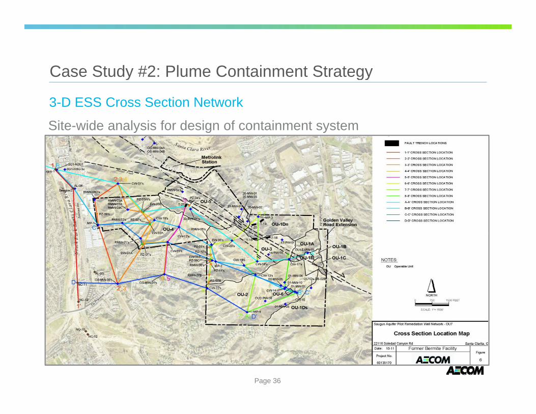
3-D ESS Cross Section Network
Site-wide analysis for design of containment system Site wide analysis for design of containment system
Page 36
Case Study #2: Plume Containment Strategy Case Study #2: Plume Containment Strategy
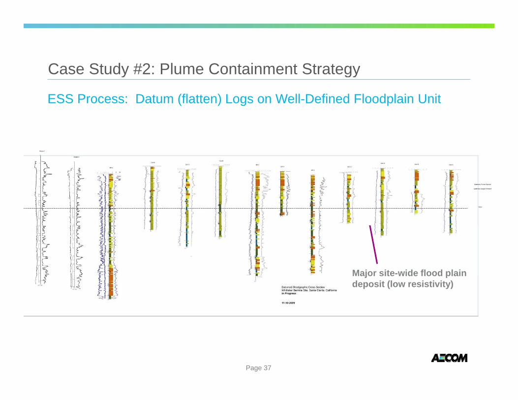
ESS Process: Datum (flatten) Logs on Well-Defined Floodplain Unit
Major site-wide flood plain Major site wide flood plain deposit (low resistivity)
Page 37
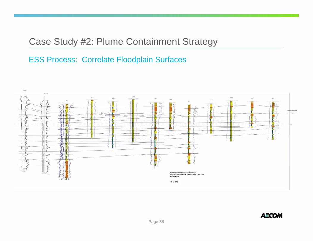
Case Study #2: Plume Containment Strategy Case Study #2: Plume Containment Strategy
ESS Process: Correlate Floodplain Surfaces
Page 38
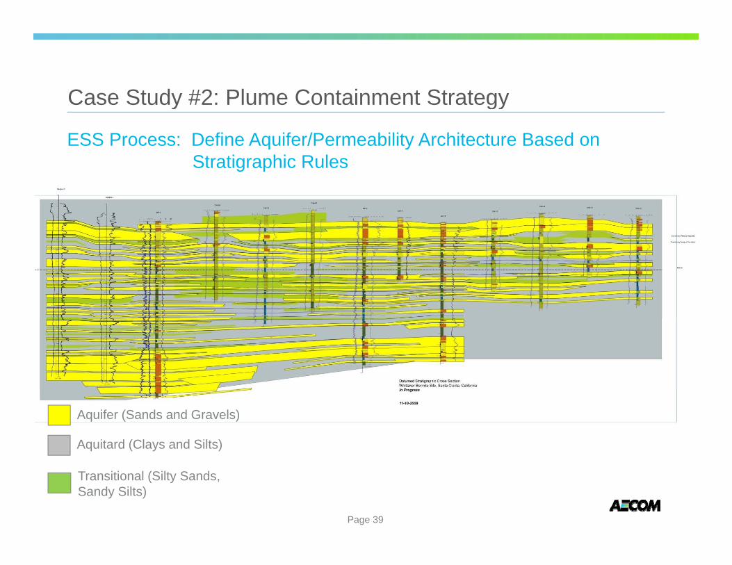
Case Study #2: Plume Containment Strategy Case Study #2: Plume Containment Strategy
ESS Process: Define Aquifer/Permeability Architecture Based on Stratigraphic Rules
Aquifer (Sands and Gravels)
Aquitard (Clays and Silts)
Transitional (Silty Sands, Sandy Silts)
Page 39
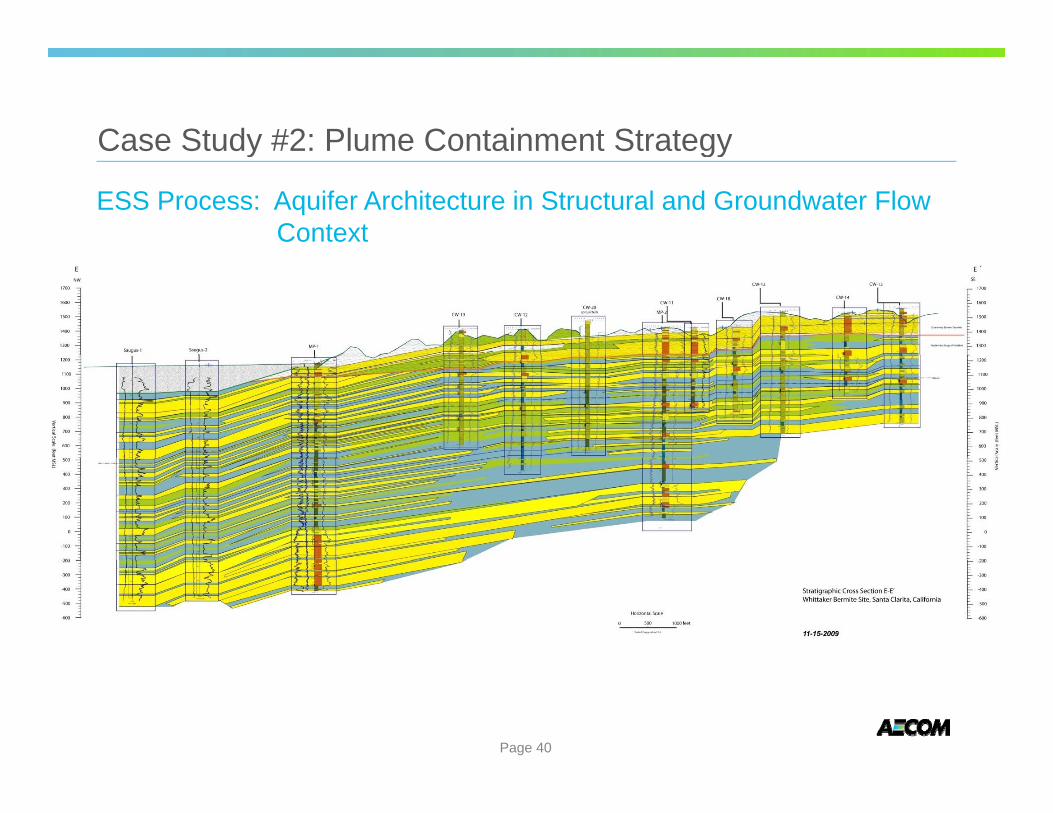
Case Study #2: Plume Containment Strategy Case Study #2: Plume Containment Strategy
ESS Process: Aquifer Architecture in Structural and Groundwater Flow Context
Page 40
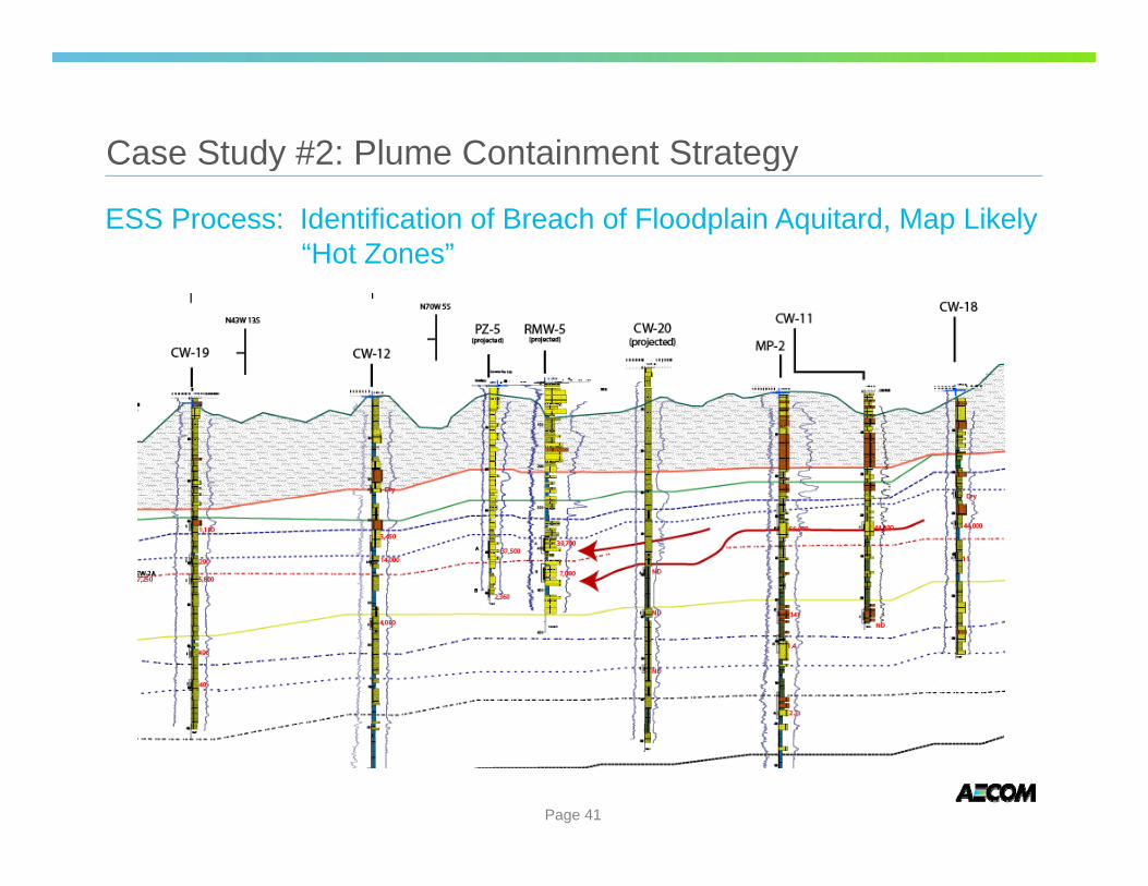
Case Study #2: Plume Containment Strategy Case Study #2: Plume Containment Strategy
ESS Process: Identification of Breach of Floodplain Aquitard, Map Likely “Hot Zones”
Page 41
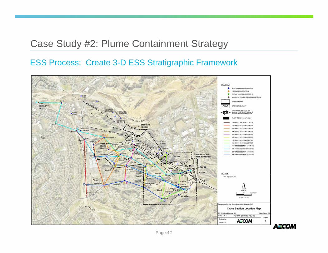
Case Study #2: Plume Containment Strategy Case Study #2: Plume Containment Strategy
ESS Process: Create 3-D ESS Stratigraphic Framework
Page 42
Page 43
Case Study #2: Plume Containment Strategy Case Study #2: Plume Containment Strategy
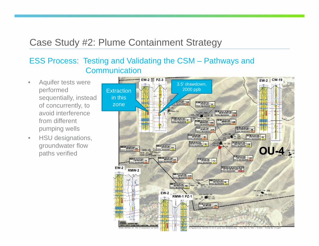
ESS Process: Testing and Validating the CSM – Pathways and Communication
• Aquifer tests wereperformedsequentially, insteadof concurrently, toof concurrently, toavoid interferencefrom differentpumping wells
• HSU designationsHSU designations,groundwater flowpaths verified
Extraction in this zone
3.5’ drawdown, 2000 ppb
30 $ 5
Page 44
Case Study #2: Plume Containment Strategy Case Study #2: Plume Containment Strategy
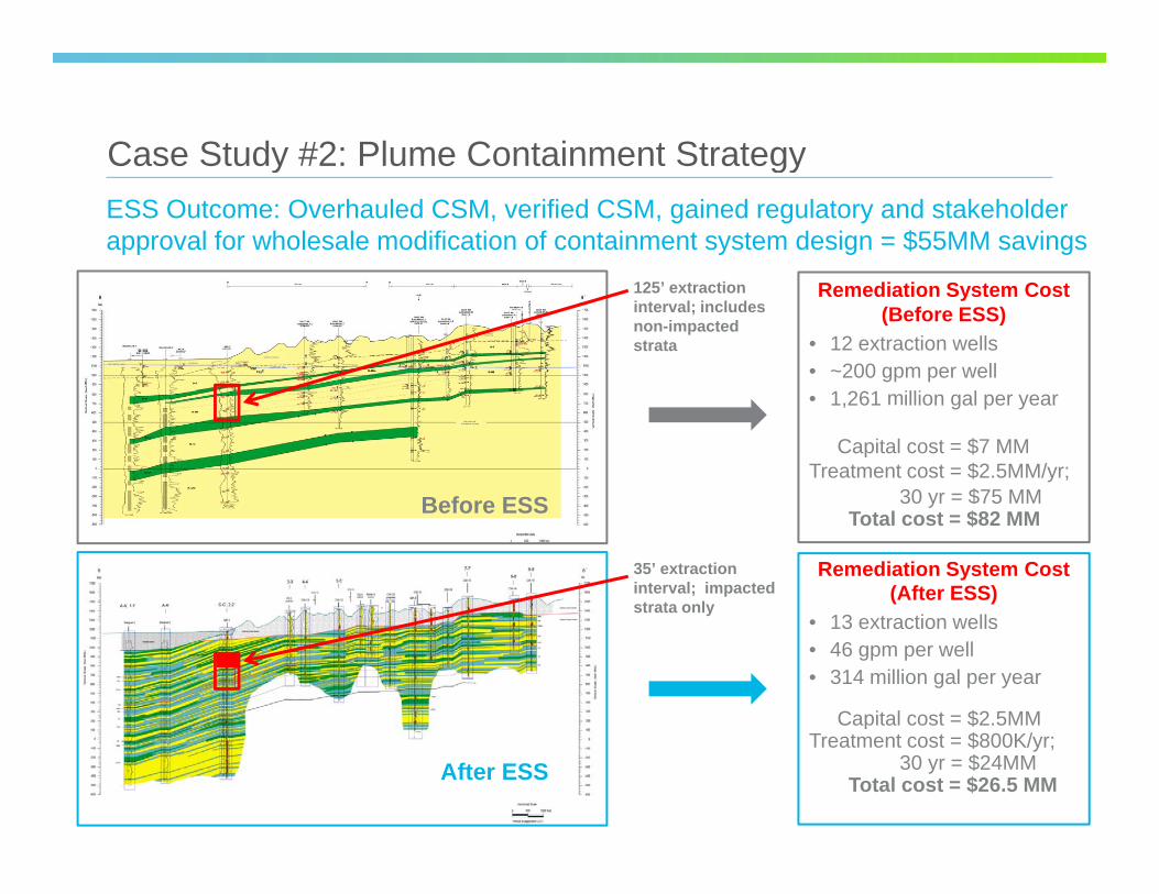
ESS Outcome: Overhauled CSM, verified CSM, gained regulatory and stakeholder approval for wholesale modification of containment system design = $55MM savings
Before ESS Before ESS
After ESS
125’ extraction interval; includes non-impacted strata
35’ extraction interval; impacted strata only
Remediation System Cost (Before ESS)
• 12 extraction wells• ~200 gpm per well
1 261 illi l• 1,261 million gal per year
Capital cost = $7 MM Treatment cost = $2.5MM/yr;
30 yr = $75 MMy Total cost = $82 MM
Remediation System Cost (After ESS)
13 t ti ll • 13 extraction wells• 46 gpm per well• 314 million gal per year
Capital cost = $2.5MMp Treatment cost = $800K/yr;
30 yr = $24MMTotal cost = $26.5 MM
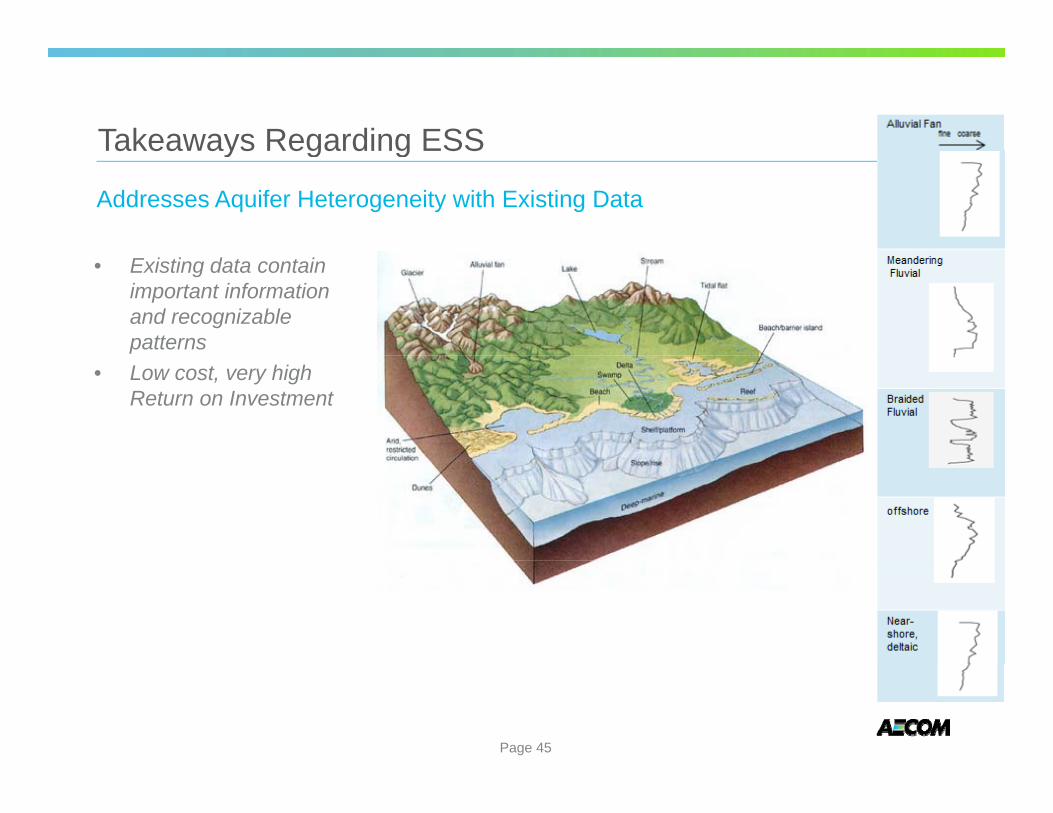
Takeaways Regarding ESSTakeaways Regarding ESS
Addresses Aquifer Heterogeneity with Existing Data
• Existing data containimportant informationand recognizablepatterns
• Low cost, very highReturn on Investment
Page 45

Questions & AnswersQuestions & Answers
Rick Cramer, M.S., P.G. Mike Shultz, PhD [email protected]@aecom.com [email protected]@ (714) 689-7264 (925) 446-3841
Page 46