foraging ecology and diet analysis of australian sea lions
TRANSCRIPT

1
Foraging ecology and diet analysis of Australian sea lions
Final Report to the Department of the Environment and Water Resources Simon D. Goldsworthy1, Kristian J. Peters1,2,3 and Brad Page1 1 South Australian Research and Development Institute (Aquatic Sciences), PO Box 120, Henley Beach, South Australia 5022 2 South Australian Research and Development Institute (Sustainable Systems – Plant and Soil Health), GPO Box 397, Adelaide South Australia 5001 3 School of Earth and Environmental Sciences, University of Adelaide, Adelaide, South Australia 5005
2
Foraging ecology and diet analysis of Australian sea lions Simon D. Goldsworthy, Kristian J. Peters, Brad Page (editors) South Australian Research and Development Institute SARDI Aquatic Sciences 2 Hamra Avenue West Beach SA 5024 Telephone: (08) 8207 5400 Facsimile: (08) 8207 5481 http://www.sardi.sa.gov.au/ Disclaimer The authors warrant that they have taken all reasonable care in producing this report. The report has been through the SARDI Aquatic Sciences internal review process, and has been formally approved for release by the Chief Scientist. Although all reasonable efforts have been made to ensure quality, SARDI Aquatic Sciences does not warrant that the information in this report is free from errors or omissions. SARDI Aquatic Sciences does not accept any liability for the contents of this report or for any consequences arising from its use or any reliance placed upon it. Copyright Department of the Environment and Water Resources, South Australian Research and Development Institute – Aquatic Sciences and The University of Adelaide 2007. This work is copyright. Apart from any use as permitted under the Copyright Act 1968, no part may be reproduced by any process without prior written permission from the author. Printed in Adelaide, November 2007 SARDI Aquatic Sciences Publication Number F2007/001024-1 SARDI Research Report Series No. 251 Editors: Simon D. Goldsworthy, Kristian J. Peters, Brad Page Reviewers: Paul Rogers and David Schmarr Approved by: Tim M. Ward
Signed: Date: 15 November 2007 Circulation: Public Domain

TABLE OF CONTENTS 3
LIST OF FIGURES...................................................................................................................5 LIST OF TABLES ..................................................................................................................10 EXECUTIVE SUMMARY .......................................................................................................12 INTRODUCTION....................................................................................................................15 NEED .....................................................................................................................................17 AIMS AND OBJECTIVES OF THE REPORT........................................................................18 THE SPATIAL DISTRIBUTION OF FORAGING EFFORT IN AUSTRALIAN SEA LION
POPULATIONS IN CLOSE PROXIMITY TO AREAS OF HIGH CATCH AND EFFORT IN THE SA ROCK LOBSTER AND SHARK GILL-NET FISHERIES...................................19 INTRODUCTION ...................................................................................................................19 METHODS...........................................................................................................................22
Capture, restraint and anaesthesia ................................................................................22 Data collection................................................................................................................22 Data analyses.................................................................................................................23
RESULTS............................................................................................................................26 DISCUSSION .......................................................................................................................31
RISK-ASSESSMENT OF SEAL INTERACTIONS IN THE SOUTH AUSTRALIAN ROCK LOBSTER AND GILL-NET SECTOR OF THE SOUTHERN AND EASTERN SCALEFISH AND SHARK FISHERY ..............................................................................35 INTRODUCTION ...................................................................................................................35 METHODS...........................................................................................................................36
Seal distribution, population size and population viability analysis.................................36 Spatial and temporal distribution of fishing effort............................................................45 Spatial and temporal overlap in fishery effort and seal foraging effort ...........................45
RESULTS............................................................................................................................48 Population distribution and size......................................................................................48 Distribution of seal foraging effort...................................................................................48 Distribution of fishing effort .............................................................................................49 Spatial overlap in fishing and seal foraging effort...........................................................51 Population viability analysis............................................................................................55 Spatial distribution of subpopulation risk category .........................................................58 Fishery bycatch scenarios ..............................................................................................58 Spatial distribution of historic bycatch: gill-net sector SESSF ........................................59 Spatial and temporal distribution of historic bycatch: gill-net sector SESSF ..................59 MFA bycatch scenarios: gill-net sector SESSF ..............................................................60 Subpopulation PVA with bycatch scenarios: gill-net sector SESSF ...............................60 Spatial distribution of historic bycatch: SA Rock lobster fishery .....................................64 Spatial and temporal distribution of historic bycatch: SA Rock lobster fishery ...............64 MFA bycatch scenarios: SA Rock lobster fishery...........................................................65 Subpopulation PVA with bycatch scenarios ...................................................................65
DISCUSSION .......................................................................................................................69 Study limitations .............................................................................................................69 Seal population data.......................................................................................................69 Foraging models and fishing effort .................................................................................70 Assessment of risks to ASL............................................................................................71 Evaluating the risk posed by SESSF gillnet sector.........................................................72 Evaluating the risk posed by SA RLF.............................................................................74 Potential to develop risk management tools...................................................................75 Conclusions and recommendations ...............................................................................76

TABLE OF CONTENTS 4
DEVELOPING MOLECULAR DNA TECHNIQUES TO DETERMINE THE DIET OF AUSTRALIAN SEA LIONS ............................................................................................111 INTRODUCTION .................................................................................................................111 METHODS.........................................................................................................................113
Trial animals and feeding trial enclosures ....................................................................113 Trial duration and diet protocols ...................................................................................113 Adult male experimental diet and female control diet...................................................115 Collection and storage of faecal samples.....................................................................117 Prey morphological analysis.........................................................................................117 Faecal DNA extraction..................................................................................................118 Prey tissue DNA extractions.........................................................................................118 Primer development .....................................................................................................119 Primer optimisation and Qualitative Standard PCR amplification.................................119 Quantitative PCR amplification - Real time PCR..........................................................120 Cloning and sequencing...............................................................................................121
RESULTS..........................................................................................................................121 Prey remains from sample collections..........................................................................121 Primer assessment.......................................................................................................122 Identification of novel prey- PCR amplification success rates ......................................123 Quantitative estimates and diet comparison.................................................................124
DISCUSSION .....................................................................................................................128 Morphological assessment of hard-prey remains.........................................................128 DNA assessment of diet – Standard PCR and quantitative PCR.................................130 Conclusions..................................................................................................................134
RECOMMENDATIONS FOR FURTHER RESEARCH........................................................135 BENEFITS AND ADOPTION...............................................................................................136 FURTHER DEVELOPMENT................................................................................................137 REFERENCES.....................................................................................................................137 APPENDIX ...........................................................................................................................148

FIGURES 5
LIST OF FIGURES
Figure 1. Location and relative size of ASL breeding colonies (grey circles are scaled based
on pup production per breeding season) in South Australia.......................................17 Figure 2. Geographic distribution of the amount of time spent in 1 km2 cells by lactating
female ASL that were satellite-tracked from South Page Island (n = 10). Dark
grey/black areas indicate regions of relatively high foraging effort. SESSF MFAs are
shown and numbered. ................................................................................................27 Figure 3. Geographic distribution of the amount of time spent in 1 km2 cells by lactating
female ASL that were satellite-tracked from South Page Island (n = 10). Dark
grey/black areas indicate regions of relatively high foraging effort. SARLF MFAs are
shown and numbered. ................................................................................................27 Figure 4. Geographic distribution of the amount of time spent in 1 km2 cells by lactating
female ASL that were satellite-tracked from Olive Island (n = 12). Dark grey/black
areas indicate regions of relatively high foraging effort. SESSF MFAs are shown and
numbered. ..................................................................................................................28 Figure 5. Geographic distribution of the amount of time spent in 1 km2 cells by lactating
female ASL that were satellite-tracked from Olive Island (n = 12). Dark grey/black
areas indicate regions of relatively high foraging effort. SARLF MFAs are shown and
numbered. ..................................................................................................................28 Figure 6. Gill-net sector SESSF Marine Fishing Areas (MFAs) off South Australia for which
catch and effort data have been recorded since 1973. ..............................................79 Figure 7. SARLF fishery Marine Fishing Areas (MFAs) off South Australia for which catch
and effort data have been recorded since 1970. ........................................................79 Figure 8. Map of South Australia and the eastern Great Australian Bight (GAB) indicating the
location of ASL (closed circles) and New Zealand fur seal (open squares) breeding
sites. Black squares indicate sympatric breeding locations........................................80 Figure 9. Estimated distribution of foraging effort (seal days.year-1) of ASL pups in South
Australia. The line indicates the edge of the continental shelf (200m). ......................81 Figure 10. Estimated distribution of foraging effort (seal days.year-1) of ASL juveniles in
South Australia. The line indicates the edge of the continental shelf (200m). ............81 Figure 11. Estimated distribution of foraging effort (seal days.year-1) of ASL sub-adult males
in SA. The line indicates the edge of the continental shelf (200m).............................82 Figure 12. Estimated distribution of foraging effort (seal days.year-1) of ASL adult females in
South Australia. The line indicates the edge of the continental shelf (200m). ............82 Figure 13. Estimated distribution of foraging effort (seal days.year-1) of ASL adult males in
South Australia. The line indicates the edge of the continental shelf (200m). ............83

FIGURES 6
Figure 14. Estimated total distribution of foraging effort (seal days.year-1) of ASL (age/gender
groups combined) in South Australia. The line indicates the edge of the continental
shelf (200m)................................................................................................................83 Figure 15. Temporal variation on total fishing effort in SA and adjacent Commonwealth
waters in the gillnet sector of the SESSF between 1973-2004 (A), and SARLF (B)
between 1970-2004....................................................................................................84 Figure 16. Distribution of fishing effort in the SA component of the gill-net sector of the
SESSF, 1973-76.........................................................................................................85 Figure 17. Distribution of fishing effort in the SA component of the gill-net sector of the
SESSF, 1977-80.........................................................................................................85 Figure 18. Distribution of fishing effort in the SA component of the gill-net sector of the
SESSF, 1981-84.........................................................................................................86 Figure 19. Distribution of fishing effort in the SA component of the gill-net sector of the
SESSF, 1985-88.........................................................................................................86 Figure 20. Distribution of fishing effort in the SA component of the gill-net sector of the
SESSF, 1989-92.........................................................................................................87 Figure 21. Distribution of fishing effort in the SA component of the gill-net sector of the
SESSF, 1993-96.........................................................................................................87 Figure 22. Distribution of fishing effort in the SA component of the gill-net sector of the
SESSF, 1997-00.........................................................................................................88 Figure 23. Distribution of fishing effort in the SA component of the gill-net sector of the
SESSF, 2001-04.........................................................................................................88 Figure 24. Distribution of fishing effort in the SA component of the gill-net sector of the
SESSF, 1973-2004.....................................................................................................89 Figure 25. Mean annual distribution of fishing effort in the SA component of the gill-net sector
of the SESSF, 1973-2004...........................................................................................89 Figure 26. Mean annual distribution of fishing effort in the SARLF, 1970-74.........................90 Figure 27. Mean annual distribution of fishing effort in the SARLF, 1975-79.........................90 Figure 28. Mean annual distribution of fishing effort in the SARLF, 1980-84.........................91 Figure 29. Mean annual distribution of fishing effort in the SARLF, 1985-89.........................91 Figure 30. Mean annual distribution of fishing effort in the SARLF, 1990-94.........................92 Figure 31. Mean annual distribution of fishing effort in the SARLF, 1995-99.........................92 Figure 32. Mean annual distribution of fishing effort in the SARLF, 2000-04.........................93 Figure 33. Distribution of total fishing effort in the SARLF, 1970-2004. .................................93 Figure 34. Mean annual distribution of fishing effort in the SARLF, 1970-2004.....................94 Figure 35. Overlap index in ASL foraging effort and SESSF gill-net fishing effort. ................94 Figure 36. Overlap index in ASL foraging effort and SARLF fishing effort. ............................95
FIGURES 7
Figure 37. Overlap index between adult female ASL foraging effort and SESSF gill-net
fishing effort. ...............................................................................................................95 Figure 38. Overlap index between adult female ASL foraging effort and SARLF fishing effort.
....................................................................................................................................96 Figure 39. Overlap index between adult male ASL foraging effort and SESSF gill-net fishing
effort. ..........................................................................................................................96 Figure 40. Overlap index between adult male ASL foraging effort and SARLF fishing effort.97 Figure 41. Overlap index between sub-adult male ASL foraging effort and SESSF gill-net
fishing effort. ...............................................................................................................97 Figure 42. Overlap index between sub-adult male ASL foraging effort and SARLF fishing
effort. ..........................................................................................................................98 Figure 43. Overlap index between juvenile ASL foraging effort and SESSF gill-net fishing
effort. ..........................................................................................................................98 Figure 44. Overlap index between juvenile ASL foraging effort and SARLF fishing effort. ....99 Figure 45. Overlap index between ASL pup foraging effort and SESSF gill-net fishing effort.
....................................................................................................................................99 Figure 46. Overlap index between ASL pup foraging effort and SARLF fishing effort. ........100 Figure 47. Estimated proportion of ASL subpopulations that achieve quasi-extinction as a
function of the number of additional pre-recruit female mortalities/subpopulation/year.
Three scenarios are given, based on the increasing (r=0.05), stable (r=0.00) and
declining (r=-0.01) population models. .....................................................................100 Figure 48. Simulated example of how the stage (age) at which mortalities are taken affects
the rate of population change. In this example a subpopulation of 1,000 female ASL
has 20 females removed from a particular age-group each year for 50 reproductive
cycles (75 years), using the stable population model (r=0). The rate of population
decline resulting from each scenario is presented, fitted with a 4th order polynomial
curve. The example demonstrates how the rate of decline is affected by the age-
group of females removed from the population. The greatest rates of decline are
achieved when 4.5-6, 6-7.5 and 7.5-9 age-group females are removed. .................101 Figure 49. Bray-Curtis similarity matrix dendrogram of SA ASL subpopulations, which are
clustered according to percentage similarity of quasi-extinction risk (from PVA
outputs). Four main groups are identified as the different Risk Categories
(dendrogram produced using Primer V5.2.2). ..........................................................102 Figure 50. Estimated proportion of historic bycatch (broken down by seal sex) accounted for
by each SA ASL subpopulation in the SESSF gillnet sector (top plot) and the SARLF
(bottom plot). ............................................................................................................103
FIGURES 8
Figure 51. Estimated proportion of historic bycatch (broken down by seal sex) accounted for
by regional groupings of SA ASL subpopulations in the SESSF gillnet sector (top plot)
and the SARLF (bottom plot)....................................................................................104 Figure 52. Estimated proportion of historic bycatch (broken down by seal sex) (1973-2004) in
SA for ASL accounted for by each SESSF gillnet sector MFA.................................105 Figure 53. Estimated proportion of historic (1970-2004) bycatch (broken down by sex) in SA
for ASL accounted for by each SA RLF MFA. ..........................................................105 Figure 54. Estimated temporal change in the proportion of historic (1973-2004) SA SESSF
gillnet sector bycatch, of ASL from different geographic regions. ............................106 Figure 55. Hypothetical temporal change in the numbers of historic (1973-2004) SA SESSF
gillnet sector bycatch, of ASL from different geographic regions. Numbers based on a
hypothetical bycatch rate of 0.005 seals/km of net-lift. .............................................106 Figure 56. Estimated temporal change in the proportion of historic (1970-2004) SA RLF
bycatch, of ASL from different geographic regions...................................................107 Figure 57. Hypothetical temporal change in the numbers of historic (1970-2004) SA RLF
sector bycatch, of ASL from different geographic regions. Numbers based on a
hypothetical bycatch rate of 0.2 seals/1,000 pot-lifts................................................107 Figure 58. Estimated temporal change in the proportion of historic (1973-2004) SA SESSF
gillnet sector bycatch, from the six major contributing MFAs for ASL. .....................108 Figure 59. Hypothetical temporal change in the numbers of historic (1973-2004) SA SESSF
gillnet sector bycatch, from the six major contributing MFAs for ASL . Numbers based
on a hypothetical bycatch rate of 0.005 seals/km of net-lift. .....................................108 Figure 60. Estimated total number of ASL and average bycatch rate required to place
different ASL subpopulations into different risk categories in SA component of (top
plot) the SESSF gillnet sector (1973-2004 mean fishing effort) and (bottom plot) the
SA RLF (1970-2004 mean fishing effort). The bycatch number refers to the total
number seals caught per year, of which about 52% are female, which are apportioned
among the 38 subpopulations based on fishery-seal interaction probabilities. ........109 Figure 61. Estimated temporal change in the proportion of historic (1970-2004) SARLF
bycatch, from the major contributing MFAs for ASL. ................................................110 Figure 62. Hypothetical temporal change in the numbers of historic (1970-2004) SA RLF
bycatch, from major contributing MFAs for ASL. Numbers based on a hypothetical
bycatch rate of 0.2 seals/1,000 pot-lifts. ...................................................................110 Figure 63. Feeding trial duration (days) and meals fed (%) during mornings (M1) and
evenings (M2) to the male (A) and female (B) ASL at the Adelaide Zoo between
January and February 2006. Arrows indicate the control periods (only fish and no
novel prey). Novel prey and fish introduced into the diet (hashed columns) for 4
weeks. Values above columns are number of days that each diet was fed. ............114

FIGURES 9
Figure 64. Prey species contributions (%) in the 6kg diet fed to the ASL male (A) and female
(B). A, B, C, and D are experimental diets consisting of novel prey; squid and shark,
combined with 2 fish species, including tommy rough and striped perch. The female
diet (B) was tommy rough (3kg) and striped perch (3kg) in equal proportions.
Columns (1, 2) are normal diets (2 fish species and no novel prey) to compare DNA
detection signals of novel prey fed during experimental diets A, B, C, and D. Values
above columns are number of days fed for each diet...............................................116 Figure 65. Standard curve from 8 Lambda (λ) DNA diluted standards (0 ng/μl to12 ng/μl) and
PicoGreen counts. Series dilutions (0-200000 fg/μl) of DNA (extracted from shark and
squid tissue) are quantified against the known (λ) DNA. Relative amounts of gummy
shark and squid dsDNA within faecal samples are determined against these values.
..................................................................................................................................120 Figure 66. Agarose gel of PCR amplification products showing detection of mtDNA by
primers Sepio71c and Gummy71c from DNA recovered from 28 male faeces. Scats
represented by numbers 1-28 were not tested in chronological order of collection, to
remove scoring bias. Circled numbers denote scats collected during each diet week
(A = 12, 18 and 22, B = 11 and 17, C = 16, and D = 2, 6, 7, 9, 13, 23, 25, 28) and
numbers in parenthesis are the contribution (% wet weight/kg) of novel prey fed
during the 6kg daily diet. Positive controls of target species are represented by circled
S (top plot) and circled G (bottom plot). H indicates negative controls for PCR
reaction testing for cross contamination. ..................................................................126

TABLES 10
LIST OF TABLES
Table 1. Length and girth, duration of satellite transmitter deployments, maximum distance
reached and average bearing travelled of individual ASL from Olive Island (n = 12)
and South Page Island (n = 10)..................................................................................29 Table 2. Comparison of the: 1) distributions of foraging effort, 2) mean depths used, 3)
proportional overlap with fishing effort (rocklobster: pot-lifts.year-1, shark: km net-
lifts.year-1) based on satellite tracking and distance-based models (Goldsworthy and
Page 2007) for each MFA. The differences between using satellite tracking data and
modelled data are shown. ..........................................................................................32 Table 3. Summary of estimates of pup production per breeding cycle for ASL breeding sites
(subpopulations) in South Australia, including the census date, source of information
and location. Only colonies where 5 or more pups have been reported are listed. Data
were current in April 2006...........................................................................................39 Table 4. Simplified hypothetical life-tables for ASL, including age-specific survival (S), and
numbers (N) per stage. Numbers are based on pup production estimates from Tables
3 and 4, assuming a 1:1 sex-ratio at birth. .................................................................40 Table 5. Leslie Matrix for ASL populations. The first row indicates the stage (age) of females
in years. The second row indicates stage-specific fecundity (proportion of female
pups born to each female per stage) and the diagonal cells denote stage-specific
survival (proportion of the previous stage surviving to the next stage) (note final stage
25.5 has a survival of 0). ............................................................................................43 Table 6. Mean estimated foraging range, proportion of time at sea and estimated foraging
effort (seal days.year-1) for different age/gender groups for ASL populations . ..........46 Table 7. Estimated mean foraging heading (and sd) for adult male ASL based on satellite
tracking studies at several locations in SA (Goldsworthy et al. unpublished data).....47 Table 8. Annual fishing effort (km net-lifts.year-1) for the 29 SA MFAs of the gill-net sector of
the Commonwealth SESSF, spanning 32 years between 1973 and 2004.................50 Table 9. Annual fishing effort (x1,000’s pot-lifts.year-1) for the 19 Marine Fishing Areas
(MFAs) of the SARLF, spanning 35 years between 1970 and 2004 ..........................52 Table 10. Average percentage fishing effort among all MFAs in the SESSF gill-net sector and
SARLF, relative to the estimated percentage of foraging effort by different age/sex
classes of ASL within each MFA of each fishery. ‘Outside’ refers to the percentage of
seal foraging effort that occurs outside the listed MFAs.............................................54 Table 11. Summary of population viability analysis (PVA) for ASL subpopulations in South
Australia. The table presents results from simulations assessing the level of additional
female pre-recruit mortality (modelled as annual removal of 1.5 year olds) required to

TABLES 11
place individual subpopulations into different risk categories (E+C= endangered and
critical, Extinct = quasi-extinct), based on the three population trajectory scenarios
(stable r= 0.00, decreasing r =-0.01, and increasing r =0.05). Qt represents quasi-
extinction time (years). The pup production of each subpopulation is given (see Table
3) and subpopulations are ranked according to risk...................................................62 Table 12. Comparison of the proportion of subpopulations of ASL reaching quasi-extinction
subject to increasing additional female mortality, under five scenarios of different age-
groups subjected to mortality. The age-groups are 0-1.5, 1.5-3, 3-4.5, 4.5-6, and 6-
7.5 years. Calculations are based on the stable population model (r=0)....................63 Table 13. Summary of PVA outcomes for ASL subpopulations, grouped in risk categories..64 Table 14. Hypothetical ASL bycatch scenarios in the gillnet sector of the SESSF off SA.
Average (1973-2004) annual fishing effort per MFA, the proportion of fishing effort
and expected proportion of ASL bycatch per MFA are presented with a range of
possible bycatch scenarios, ranging from an average of 0.0005 to 0.0400 seals per
km net-lift/year. Individual MFA bycatch rates are given for each scenario. ..............66 Table 15. Hypothetical ASL bycatch scenarios in the SA RLF. Average (1970-2004) annual
fishing effort per MFA, the proportion of fishing effort and expected proportion of ASL
bycatch per MFA are presented. ...............................................................................68 Table 16. Frequency of occurrence (FOO) and numerical abundance (NA) of diagnostic hard
remains (otoliths) identified from scats (n = 28) collected from the male ASL during
feeding trials. Diagnostic remains from squid were not recovered. ..........................122 Table 17. PCR primers tested in standard and real-time quantitative PCR for detecting squid
and shark in sea lion scats. Successful primers (+) in bold. All other primers amplified
target taxon DNA but not prey DNA from faeces (-).Shark refers to M. antarcticus and
squid refers to S. australis. a Unpub. data current study, b Jarman et al. (2006), c
Deagle et al. (2005), d Casper et al. (2007), e Jarman et al. unpub. data..................123 Table 18. Total mass ingested (TMI), mass recovered (MR) (wet weight/kg) and percent (%)
of mass recovery reconstructed for the total number of fish recovered (total otoliths
recovered divided by 2) from (n) scats for Diet A, B, C, D and controls. Post trial
controls were pooled. Mass estimates were reconstructed from weight length data
collected from 100 fresh specimens of each fish species. .......................................125 Table 19. PCR amplification results (+) presence (-) absence for standard and real-time
quantitative PCR (qPCR) values (fg/μl) for the detection of squid and gummy shark
mtDNA from scats collected from a captive male ASL during feeding trials at the
Adelaide Zoo. Scat samples represented in chronological order of collection while trial
day (n) indicates actual day of collection for duration of 48 days. ............................127

NON-TECHNICAL SUMMARY 12
EXECUTIVE SUMMARY
Recent Commonwealth Department of the Environment and the Heritage (DEH) Ecological
Sustainable Development (ESD) assessments of the South Australian (SA) rock lobster
(SARLF) and southern and eastern scalefish and shark fishery (SESSF) identified
interactions with protected species (particularly seals), as one of the key bycatch issues. The
issues are most relevant to SA waters where threatened Australian sea lion (ASL)
populations are located, and where un-quantified interactions between seals and the SARLF
and gillnet sector of the SESSF fisheries are known to occur. Recommendations from fishery
ESD assessments, fishery Bycatch Action Plans, and a recently drafted Recovery Plan for
the ASL, have all identified the importance of assessing and mitigating interactions between
seals and commercial fisheries. This study provides a desk-top risk-assessment of seal
fisheries interactions in the SARLF and gillnet sector SESSF in SA and adjacent waters, and
makes recommendations on future research and management responses.
A review of the PIRSA and AFMA fishery logbooks identified the major constraint to the
assessment of bycatch risk to seal subpopulations was the absence of quantitative data on
bycatch rates in both the gillnet sector SESSF and SARLF. Anecdotal evidence and
entanglement data suggest there has been significant underreporting of seal interactions in
these fisheries.
In SA there are 38 ASL subpopulations that produce around 2,674 pups, with the total
population size estimated at about 10,900. However, most pup production (67%) occurs at 6
sites, hence the median pup production is very low (25.5 pups), with the majority of sites
producing small numbers of pups (60% produce <30 pups per season). Population viability
analysis (PVA) on ASL subpopulations reinforced the recent listing of the ASL as a
threatened species, by confirming that large numbers of subpopulations with low pup
production are vulnerable to extinction. PVA simulations suggested that in absence of
anthropogenic mortality, a number of ASL subpopulations will go quasi-extinct (ie the number
of adult females is too low to ensure population persistence; <10 females), but in the face of
small (1-2 additional females/year) but sustained anthropogenic mortality (eg. from fishery
bycatch), most other small subpopulations will become quasi-extinct and negative growth will
become a feature of even the largest subpopulations. There is apparent depletion (ie. very
low pup production) of a large number of subpopulations that may be indicative of
widespread subpopulation declines in the species. That such declines may be ongoing and
attributable to anthropogenic mortality (ie. fishery bycatch) is a hypothesis that requires
urgent attention.

NON-TECHNICAL SUMMARY 13
The risk of bycatch in the gillnet SESSF and SARLF were assessed based on estimates of
interaction probabilities. These were a function of the extent to which historic fishing effort
and seal foraging effort (based on foraging distribution and population models) overlap in
space and time. ASL demonstrated a high risk of significant depletion and quasi-extinction as
a result of fishery bycatch. By combining PVA outcomes with bycatch scenarios based on
interaction probabilities, this study identified the subpopulations, regions and marine fishing
areas (MFAs) most at-risk from seal bycatch.
Bycatch from the gillnet SESSF is most likely to provide the greatest risk to ASL, because of
almost complete spatial overlap in fishing effort with ASL foraging effort, it is a year-round
fishery with relatively high fishing effort that can potentially interact with all ASL age-classes.
The impact from SARLF is likely to be less because there is less overlap in fishing effort with
ASL foraging effort, fishing is restricted to seven months of the year (November-May) and
bycatch is likely to be restricted to pups and juvenile seals. However, the potential additive
and interactive impacts posed by combined bycatch in these fisheries could be significant.
Results from this study suggest the two fisheries investigated lend themselves to different
mitigation approaches to addressing seal bycatch issues. In the gillnet SESSF, gear
modification options are limited, but spatial management of fishing effort may provide a range
of risk-reduction options, but would need to be coupled with independent observer bycatch
data to demonstrate and justify the benefits from different closure options. In contrast, there
are significant options for gear modification in the SARLF, with pot-protection devices already
used in some parts of the fishery. Quantitative testing of these and alternate protection
measures (as is taking place in the WA WRLF), and industry wide adoption of best-mitigation
practices may eliminate seal bycatch in this fishery, without the need for an expansive and
costly independent observer program. Recommendations for future research are made, that
should result in the successful mitigation of seal bycatch issues and as a consequence
address the recommendations of the fishery ESD, Bycatch Action Plan, ASL Recovery Plan
and assist in the recovery of the threatened ASL.
Enhanced spatial tools for risk assessment will be required if spatial management of fishing
effort is to become a management strategy for mitigating ASL bycatch in the demersal gillnet
fishery. Such tools would provide a simple mechanism for policy makers and managers to
evaluate the benefits and costs of different spatial allocations of fishing effort, in terms of
increasing or decreasing: 1) risk to sea lion subpopulations and 2) fishery catches. However,
further development of such tools are required, because current models are limited by the

NON-TECHNICAL SUMMARY 14
absence of data on the foraging movements of sea lions in some high-risk regions, as well as
the absence of accurate fishing effort data.
Further satellite tracking of ASLs at subpopulations identified as high-risk was undertaken as
part of this study, to improve the accuracy of spatial foraging models. This pilot study
demonstrated an approach to refine assessments of sea lion interactions with commercial
fisheries, where quantitative data on interactions are not available. This approach may
enhance the spatial information on which mitigation options and decisions about spatial
management of fisheries are based. Importantly, the pilot study determined that colony-
specific information on sea lion foraging effort could be used to refine the spatial
management of fisheries when using fishing effort data that was summarised into 1 x 1
degree boxes (Marine Fishing Areas). In 2006, demersal gillnet fishers were required to
record the latitude/longitude positions of each net-set, and from July 2007, all vessels will be
fitted with satellite-linked vessel monitoring systems that will significantly improve the
resolution of fishing effort. Following these improvements to fishing effort data sets, it is
recommended that bycatch probabilities be re-estimated with colony-specific information on
seal lion foraging effort and used to model the benefits of different spatial-management
scenarios that could include area-closures, and reductions or redistributions of fishing effort.
The diet of the ASL is currently poorly understood, which hampers our understanding of their
key prey species, habitats and trophic interactions with fisheries. Traditional faecal analysis
techniques have proven ineffective in ASL because most prey remains are completely
digested. We conducted a feeding trial on captive ASL to determine whether faecal DNA
analysis could be used to quantify sea lion diet. This study demonstrated that analysis of
faecal DNA can detect the presence of sea lion prey DNA, despite no identifiable prey hard
parts being recovered from the same scats. The results from our experiments also
demonstrate that DNA extracted from ASL scats is highly degraded, because we could not
detect prey DNA using molecular primers more than 100 base pairs in length. Quantitative
PCR indicated that the amount of mtDNA amplified from scats was related to the amount of
novel prey ingested. Quantitative estimates determined the difference between periods of
high consumption of novel prey and low consumption of a particular prey type, but did not
pick up smaller differences in consumption rates. Interestingly, mtDNA quantitative estimates
were significantly higher for squid than shark from periods when the seal was fed in equal
proportions. These differences may be related to the concentration of DNA in the different
tissue types of each species.
KEYWORDS: SA rock lobster fishery (SARLF), gillnet sector of the South Eastern Scalefish
and Shark fishery (SESSF), Australian sea lion (ASL), bycatch

AIMS AND OBJECTIVES 15
INTRODUCTION
The Australian sea lion (ASL) Neophoca cinerea is one of five sea lion species in the world.
Sea lions form around one-third of species in the Otariidae family of seals that includes all of
the fur seals and sea lions. Over recent decades there has been growing concern over the
status of all five sea lion species. In the North Pacific Ocean, the Steller sea lion, Eumetopias
jubatus, has been declared endangered in parts of its range and is considered threatened
with extinction in other parts (Trites et al. 2007). Although the total population of California
sea lions in California and Mexico is increasing (Caretta et al. 2004), the Mexican stock is in
decline (Szteren et al. 2006). There have also been reductions in numbers of the Galapagos
subspecies of the Californian sea lion, Zalophus californianus wollebaeki (Alava and Salazar
2006) and the Japanese subspecies, Z. c. japonicus, is possibly extinct (Mate 1982).
Numbers of South American sea lions, Otaria flavescens, have reduced considerably in
recent years (Crespo and Pedraza 1991, Reyes et al. 1999, Shiavini et al. 2004), especially
in the Falkland Islands (Thompson et al. 2005). Numbers of New Zealand sea lions,
Phocarctos hookeri (Lalas and Bradshaw 2003) and ASL (McKenzie et al. 2005) have not
recovered from historic sealing and form the smallest populations of all sea lion species.
The ASL is Australia’s only endemic and least-abundant seal species. It is unique among
pinnipeds in being the only species that has a non-annual breeding cycle (Gales et al. 1994).
Furthermore, breeding is temporally asynchronous across its range (Gales et al. 1994, Gales
and Costa 1997). It has the longest gestation period of any pinniped, and a protracted
breeding and lactation period (Higgins and Gass 1993, Gales and Costa 1997). The
evolutionary determinates of this atypical life-history remain enigmatic. Recent population
genetic studies have indicated little or no interchange of females among breeding colonies,
even those separated by short (20 km) distances (Campbell 2003). The important
management implication of extreme levels of female natal site-fidelity (philopatry) is that each
colony effectively represents a closed population.
There are 73 known breeding locations for ASLs, 47 of which occur in South Australia where
the species is most numerous (80% of pups counted), with the remainder (26 colonies)
occurring in Western Australia (McKenzie et al. 2005). The species was subject to sealing in
the late 18th, the 19th and early 20th centuries, resulting in a reduction in overall population
size and extirpation of populations in Bass Strait and other localities within its current range.
Total pup production for the entire species during each breeding cycle has been estimated at
about 2,500 with an estimated overall population size based on a demographic model

AIMS AND OBJECTIVES 16
developed by Goldsworthy et al (2003), of around 9,800 (McKenzie et al. 2005). A re-
analysis of this demographic model, in conjunction with improved estimates of pup
production for some sites, has increased estimates of the SA pup production to about 2,700
per breeding cycle and the size of the ASL population in SA to about 10,900 individuals
(Goldsworthy and Page 2007). Based on pup production estimates of 709 for WA sites
(Goldsworthy et al. 2003), the total pup production for the species is currently estimated at
about 3400 per breeding cycle, with an estimated overall population estimate of around
14,000 (Goldsworthy, unpublished data). The life tables associated with the population model
produced population estimates that were 4.08 times that of pup production (Goldsworthy and
Page 2007), which is about mid-point of the range expected for pinniped populations
(Harwood and Prime 1978).
There are 39 ASL breeding sites in SA, when the criterion for classification as a breeding
colony is set at ≥ 5 pups present per breeding cycle (McKenzie et al. 2005, Fig. 1). Of these,
only six (16%) produce more than 100 pups, and these account for 67 % of the State’s pup
production. The largest population is Dangerous Reef in Southern Spencer Gulf (585 pups),
followed by The Pages (577 pups) in Backstairs Passage between Kangaroo Island and
mainland Australia. The next largest populations are Seal Bay (214 pups) on Kangaroo
Island, West Waldegrave (157 pups) and Olive Islands (131 pups) off the west coast of the
Eyre Peninsula, and Purdie Island (132 pups) in the Nuyts Archipelago (summarised in
Goldsworthy and Page 2007). The median pup production for SA colonies is 25.5 per colony,
with 60% of breeding sites producing fewer than 30 pups per season, 42 % fewer than 20
pups, and 13% fewer than 10 pups (Goldsworthy and Page 2007). These analyses do not
take into account at least another 11 breeding sites (termed ‘haul-out sites’ with occasional
pupping), where fewer than 5 pups have been recorded at some time (McKenzie et al. 2005).
The ASL is Australia’s only endemic pinniped, and was recently listed under the Environment
Protection and Biodiversity Conservation Act as Threatened, 'Vulnerable' category (gazetted
14 Feb 2005), and a recovery plan is has been drafted by Commonwealth DEH.
Although the pre-harvested population size of the ASL is unknown, the overall population is
still believed to be in recovery. Unlike Australian fur seal, Arctocephalus pusillus doriferus
and New Zealand fur seal, Arctocephalus forsteri populations, which have been recovering
rapidly throughout southern Australia, there is a general view that the overall population
recovery of the ASL appears to be limited, and it is unclear why.

AIMS AND OBJECTIVES 17
kilometres
0 100 200
Figure 1. Location and relative size of ASL breeding colonies (grey circles are scaled based
on pup production per breeding season) in South Australia.
NEED
Provisions of the Commonwealth Environment Protection and Biodiversity Conservation Act
(EPBC Act), require strategic assessment of fisheries against the principles of ESD including
the need to monitor, assess and, if necessary, mitigate the interactions of fisheries with
protected species (Fletcher et al. 2002).
In both the SARLF and gillnet sector of the SESSF there are considerable policy and
research requirements relating to fishery interactions with sea lions that need to be
undertaken in order to fulfil recommendations detailed in recent Bycatch Action Plans and
ESD Assessments (Goldsworthy and Page 2007).
The Australian Governments’ National Seal Action Plan requires the estimation of sea lion
bycatch in gillnet, trawl, trap, dropline and longline fisheries and quantification of interactions
with fishing equipment.
ASL are listed as protected species under the Commonwealth EPBC Act, and are known to
interact with lobster and gillnet fisheries.
Pup numbers
400 to 650 (2)
200 to 400 (1)
100 to 200 (3)50 to 100 (5)25 to 50 (6)1 to 25 (26)

AIMS AND OBJECTIVES 18
Methods for assessing, monitoring and mitigating the interactions of ASL with lobster and
gillnet fisheries are needed urgently. This need is greatest in South Australia, where:
1. The majority of subpopulations of the ASL occur, and where declining populations have
been identified;
2. A valuable ($70 M) fishery for southern rock lobster (Jasus edwardsii) is located;
3. Un-quantified interactions between ASL and the SARLF and gillnet sector of the SESSF
fisheries are known to occur.
The need to assess the interactions between these fisheries and ASL is particularly pressing
because it:
1. Is Australia’s only endemic pinniped;
2. May be more vulnerable to fishery-induced mortality than other species;
3. Is mainly confined to South Australia, with ~80% of pup production occurring in the State;
4. Has recently been listed as Threatened (Vulnerable Category) under Commonwealth
EPBC Act.
AIMS AND OBJECTIVES OF THE REPORT
The aims of this report are to:
1. Use satellite tracking methods to assess the spatial distribution of foraging effort in ASL
populations in close proximity to areas of high catch and effort in the SARLF and shark gill-
net fisheries;
2. Assess the degree of spatial overlap in ASL foraging space and catch and effort in the SA
rock lobster and shark gill-net fisheries;
3. Provide advice to DEH on the risks posed by commercial fisheries that overlap with the
foraging space of sea lions and provide advice on the spatial management of the fisheries;
4. To develop novel, quantitative PCR-based faecal DNA assessment methods that can be
used to identify key prey taxa and quantify their contribution in the diet;
5. To calibrate the accuracy of the method by undertaking a feeding trial on captive seals.
This report addresses objective 1 as separate chapter and the following two chapters
address objectives 2-3 and 4-5, respectively.

SEA LION FORAGING EFFORT IN AREAS OF HIGH FISHERIES EFFORT 19
THE SPATIAL DISTRIBUTION OF FORAGING EFFORT IN AUSTRALIAN SEA LION POPULATIONS IN CLOSE PROXIMITY TO AREAS OF HIGH CATCH AND EFFORT IN THE SA ROCK LOBSTER AND SHARK GILL-NET FISHERIES
Derek J. Hamer 1,2, Brad Page1 and Simon D. Goldsworthy1 1 South Australian Research and Development Institute (Aquatic Sciences), PO Box 120, Henley
Beach, South Australia 5022 2 School of Earth and Environmental Sciences, University of Adelaide, Adelaide, South Australia
5005
Introduction
A recovery plan for the Australian sea lion (ASL) was recently drafted by NHT (NHT,
2005), after the species was listed as Vulnerable pursuant to the Environment Protection
and Biodiversity Conservation Act 1999 (EPBC Act). The decision to upgrade the
species from Conservation Dependent was based primarily on reports to DEWR
(formerly DEH and administrator of the EPBC Act), which detailed the possible
impediments to growth in ASL populations (McKenzie et al. 2005).
The recent report to DEWR identified a number of factors that might result in population
declines, with anthropogenic factors of top-down (mortality driven) origin being
considered the most likely and relevant (McKenzie et al. 2005). Direct killing, pollutants
and toxins, plus fishery by-catch and entanglement were considered as possible
contributors, although there is currently no evidence that direct killing or pollution and
toxins are contributing factors. However, a number of sources indicated that fishery by-
catch and entanglement might be a contributing mortality factor in some parts of the
range of ASL (Page et al. 2004, Goldsworthy and Page 2007). As a consequence, the
report ranked fishery by-catch and entanglement as the most important contributor to
limited growth in some populations and declines in others (McKenzie et al. 2005).
A substantial body of information exists regarding operational interactions between ASL
and southern rock lobster (Jasus edwardsii) pots and demersal gummy shark (Mustelus
antarcticus) and school shark (Galeorhinus galeus) gill-nets. The drowning of significant
numbers of ASL pups in Western Australia and juvenile Australian fur seals in Victoria in
rock lobster pots when attempting to remove either baits or rock lobster has been

SEA LION FORAGING EFFORT IN AREAS OF HIGH FISHERIES EFFORT 20
speculated over the past 30 years (Warneke 1975; Gales et al. 1994). However, recent
reports now confirm that these interactions may occur in large enough numbers to
potentially impact on the conservation of some breeding populations in Western Australia
(Campbell 2004). Anecdotal reports that operational interactions between seals and
shark fishing operations are more likely to occur in coastal waters and the admission by
one fisher who claimed to have caught about 20 ASL yearly both suggest that sea lions
also drown in shark gill-nets (Shaughnessy et al. 2003). The high incidence of ASL
entanglements in monofilament shark gill-net material on Kangaroo Island suggests that
the level of interaction with shark gill-nets may be high (Page et al. 2004).
The recent interest in the impact of commercial fisheries on ASL populations has now
confirmed that operational interactions occur with rock lobster pots and shark gill-nets. In
spite of this, their occurrence was completely absent from logbooks submitted by the
South Australian Rock Lobster Fishery (SARLF) during a recent review (Hamer 2007).
The same review found that rates of operational interactions with shark gill-net fishing
operations in the Southern and Eastern Scalefish and Shark Fishery (SESSF) were very
low, with only seven mortalities reported between 1999 and 2004. Low interaction rates
with shark gill-net fishing activities in Victorian waters were also reported in logbook
records (Walker et al. 2005). The disparity between these records and the apparent
broad scale occurrence of operational interactions between ASL and these two fisheries
suggest that there has been and is currently a high degree of underreporting in both of
these fisheries.
Commercial fisheries have been required to undergo strategic assessment pursuant to
the EPBC Act since its enactment in 2000. In particular, their activities are assessed
under Part 10, against the Guidelines for the Ecologically Sustainable Management of
Fisheries , reflecting internationally recognised principles of ecologically sustainable
development (ESD). Monitoring, assessing and mitigating operational interactions with
protected species subject to a recovery plan is the manifestation of these principals. The
requirement for this course of action was also reflected in the original listing advice for
the species, which also confirmed the need to establish a unified approach under the
recovery plan for the species with complementary threat abatement through changes in
fishing practices.
The SARLF and the gill-net sector of the SESSF have recently undergone strategic
assessment, in April 2003 and November 2002, respectively (Department of the
Environment and Heritage 2003a & b). DEWR responded by handing down a number of

SEA LION FORAGING EFFORT IN AREAS OF HIGH FISHERIES EFFORT 21
recommendations for improvement to the management of each fishery, some of which
specifically focused on operational interactions with fur seals and sea lions. In
September 2003, DEWR recommended that the SESSF gill-net sector mitigate
interactions with seals by establishing a reporting system within 12 months (18i) and
appropriate mitigation tools, such as spatial closures, within 3 years (18ii). Similarly,
DEWR responded in October 2003 to the SARLF ecological assessment by
recommending that a mandatory reporting system be established within 18 months (10)
and appropriate mitigation measures be implemented within 2 years (11).
All of the time limits associated with each DEWR recommendation for both fisheries have
now expired without action. However, the existence of each of these fisheries is
contingent on receiving an exemption to trade in a native species, pursuant to Parts 13
and 13A of the EPBC Act. Compliance to this aspect of the EPBC Act is of particular
relevance, because all declarations, agreements and decisions made in relation to such
activities pursuant to the EPBC Act are in recognition of the Convention on International
Trade in Endangered Species of Wild Fauna and Flora 1973 (CITES).
The need to address these DEH recommendations is greatest in South Australian
waters, where the majority of subpopulations of ASL occur and where declining
populations have been identified (Goldsworthy et al. 2003; Shaughnessy et al. in press).
This is particularly important while operational interactions between ASL and southern
rock lobster pot and shark gill-net fishing activities remain unquantified.
In the absence of data and quantified information regarding interaction rates,
management agencies have struggled to determine the appropriate course of action for
management of ASL. This includes justification of observer programs, which are typically
costly to industry, especially if observer effort is to be representative of fishing effort
across the fleet and its geographic range. In addition, a relatively low level of operational
interactions may have a relatively large impact on small breeding colonies, but the
impact of relatively high interaction rates adjacent to large breeding colonies may be
relatively small. How best to estimate the potential impacts of by-catch on protected
species and how to recognise the most appropriate mitigation options is a perennial
issue faced by the managers of fisheries and protected species.
A key aspect of assessing the potential threat of fishing activities on ASL populations is
to examine the extent to which they spatially utilise the marine environment and the
degree to which their efforts overlap (Goldsworthy et al. 2003). Data obtained through
SEA LION FORAGING EFFORT IN AREAS OF HIGH FISHERIES EFFORT 22
satellite telemetry will be used to determine the spatial utilisation of the marine
environment by foraging adult female sea lions from breeding colonies in close proximity
to regions of high rock lobster pot and shark gill-net fishing effort. These results are then
compared with the results of a spatial model developed by (Goldsworthy and Page
2007), to assess the level of agreement between the two sources and how a
combination of the two might be used to refine the degree of seal-fisheries overlap in
these regions. The results will assist in the implementation of the draft recovery plan, by
providing information on the degree and distribution of spatial overlap between the two
and the subsequent distribution of risk to individual populations.
Methods
Capture, restraint and anaesthesia
To determine the spatial distribution of ASL foraging effort, satellite transmitters (KiwiSat
101, Sirtrack, Havelock North, New Zealand) were deployed on sexually mature females.
This demographic was chosen, as they are most important for providing recruits to the
next generation of the population through the contribution of pups. A hoop-net was used
to initially restrain individual animals. Anaesthesia was induced and maintained using
Isoflurane® (Veterinary Companies of Australia, Artarmon, Australia), administered via a
purpose-built gas anaesthetic machine with a Cyprane Tec III vaporiser (Advanced
Anaesthetic Specialists, Melbourne, Australia). Once anaesthetised, a satellite
transmitter was then attached to the guard hairs along the mid-dorsal line, between the
fore-flippers, using a thin layer of Araldite® 2107 (Vantico, Basel, Switzerland), a flexible,
two-pack epoxy adhesive. The welfare and health of the animal was monitored
throughout the procedure, in accordance with the procedures approved separately by
Primary Industries and Resources SA (PIRSA) and University of Adelaide Animal Ethics
Committees.
Data collection
Once anaesthetised, the length (nose to tail) and mid-planar girth (from behind the fore-
flippers) of each sea lion was measured (± 1 cm). Unique numbered plastic tags
(Supertags®, Dalton, Woolgoolga, Australia) were applied to the trailing edge of each
fore-flipper of animals at breeding colonies currently included in a broader, long term
population monitoring program.

SEA LION FORAGING EFFORT IN AREAS OF HIGH FISHERIES EFFORT 23
Most satellite transmitters were recovered by recapturing animals with the hoop net.
However, animals that consistently remained very alert or close to the water, thus
reducing the likelihood of being successfully restrained in this manner, were
administered Zoletil® (~1.1 to 1.2 mg per kg) via a 1.0 cc barbless dart (Pneu-Dart®,
Pennsylvania, USA), delivered by a CO2 powered dart gun (Taipan 2000, Tranquil Arms
Company, Melbourne, Australia). The satellite transmitter was then removed by cutting
through the guard hairs immediately beneath the unit.
Data analyses
Satellite location data were obtained through Service Argos Inc. Due to the variability in
spatial quality of the information obtained, the least accurate (class Z) positions were
omitted from the analysis (Sterling and Ream 2004). Spatial analysis was conducted
using R statistical software (version 2.3.0, R Development Core Team, R Foundation for
Statistical Computing, Vienna) and the timeTrack package (version 1.1-5, M. D. Sumner,
University of Tasmania, Hobart) and were used to redistribute at-sea locations during
foraging trips (McConnell et al., 1992), based on a maximum possible horizontal speed
of 11.93 km/h (Goldsworthy et al., unpublished data).
It was assumed that all the sea lions carrying satellite transmitters would consistently
return to their colony to suckle pups, so all foraging trips were separated by haulout
periods. Precise coordinates were entered for the central location of each breeding
colony, so the beginning (when the animal departed) and end (when the animal hauled
out) of foraging trips could be estimated. Foraging trips typically started after a few days
of non-transmission and ended after the transmitter sent several high-class hits, prior to
the timer (activated by a salt water switch) temporarily turned the unit off. If a satellite
transmitter failed while an animal was at sea, that entire foraging trip was excluded from
the analyses. However, in many cases the satellite transmitter did not give any locations
after the sea lion appeared to have hauled out on land. In these cases, the following
criteria were used to estimate when the sea lion hauled out: 1) no locations were
received by satellites for > 8 hr, possibly indicating that the haulout timer had switched
off the satellite transmitter because the animal was not in the water, 2) the distance to
the colony was calculated from the last satellite location to determine if it was close to
the colony and 3) the direction of travel indicated that it was travelling toward the colony,

SEA LION FORAGING EFFORT IN AREAS OF HIGH FISHERIES EFFORT 24
Due to the inherent inaccuracy associated with the location data, determining when
foraging trips began and ended was difficult at best. We calculated the distance between
the first/last location at sea and the colony where the seal hauled out and interpolated
the start/end times based on average travel speeds between these locations. The
average travel speed of sexually mature female ASL was used in this calculation, based
on outbound (2.63 + 0.62 km/h) and inbound (6.43 + 1.29 km/h) estimates derived from
previous studies at Dangerous Reef, South Australia (Goldsworthy et al., unpublished
data).
The R statistical software and timeTrack were used to determine the number of different
1 km2 grid cells entered by each seal and the proportion of time they spent in each. We
assumed a constant horizontal speed between each filtered location and interpolated a
new position for each 15 minute block of time along the path between them. The number
of original and interpolated positions within each cell were then summed and assigned to
a central node within it. To ensure the different deployment durations recorded for
different seals did not bias comparisons, the amount of time spent in each cell was
converted to a proportion of the total time spent at sea for each individual. The
proportional values of the time spent in each 1 km2 grid cell were then plotted, using the
triangulation with a smoothing function in VerticalMapper® and MapInfo® (version 2.5 and
8.0 respectively, MapInfo Corporation, New York, USA).
Fishing effort data for the gill-net sector of the SESSF, within and adjacent to South
Australian waters, were derived from fishery logbooks obtained from the Australian
Fisheries Management Authority submitted over a 32 year period, between 1973 and
2004. Fishing effort data for the SARLF were obtained from SARDI Aquatic Sciences for
the 35 year period between 1970 and 2004. The spatial resolution of logbook data has
traditionally been poor in both of these fisheries, with management areas for both
typically following degree lines of longitude and latitude and referred to as marine fishery
areas (MFAs).
The same processing techniques used to determine the proportion of time that a seal
spent in each 1 km2 grid cell were used to determine the proportion of time spent within
each MFA, by pooling the values for all cells that fell within the boundary of each MFA.
The proportion of fishing effort (rocklobster: pot-lifts.year-1, shark: km net-lifts.year-1),
were also calculated across all MFAs adjacent to the South Australian coast. The degree
of spatial overlap between sea lions and each fishery was then calculated by multiplying

SEA LION FORAGING EFFORT IN AREAS OF HIGH FISHERIES EFFORT 25
the proportional seal foraging effort (time) in each MFA by the proportional fishing effort
in the MFAs visited by sea lions from each site.
Using the distributions of foraging effort data from satellite tracking data and the models
developed by Goldsworthy and Page (2007), the total amount of foraging effort within
each fishery MFA was calculated by summing the values for each grid cell within each
fishery MFA. The proportion of the total sea lion foraging effort (FE), which occurred
within each fishery MFA, was then derived from satellite tracking data and the models.
Based on the historical fishing effort records, the product of the proportion of (modelled
and actual) seal FE and fishing effort (F) were calculated within each MFA. The extent of
overlap between fishing effort and seal foraging (overlap index, OI, adapted from
Schoener (1968)) within each MFA was then calculated as a probability (f) by dividing
the product of the proportion of fishing effort (FFMA) and the proportion of seal foraging
effort (FEFMA) within each MFA, by the sum of all the products from all MFAs, as follows:
∑=
=
=FMANFMA
FMAFMAFMA
FMAFMAFMA
FfFEf
FfFEfOIf
1)().(
)().()(
where NFMA is the total number of MFAs
We summarised the foraging behaviour of each seal to calculate differences in the
habitats they utilised (tracking data) and the habitats that a distance-based foraging
model (Goldsworthy and Page 2007) predicted that sea lions from Olive and South Page
Island would use. The models developed by Goldsworthy and Page (2007) assumed that
seals from Olive and South Page Islands foraged within a set range from their colony,
according to the normal probability density function. We calculated the differences in the
location of actual and modelled foraging habitats based on the proportional values of
time-spent in area. We also calculated differences in the depth of habitats between the
actual and modelled distributions of sea lion foraging locations. Mean depth values for
both the actual and modelled data were weighted by the amount of time spent over each
depth. Depth data were obtained from the GeoScience Australia 1 x 1 km grid. The
depth values for each location were interpolated as functions of their distance from the
nearest nodes and assigned to each 15 min interval.

SEA LION FORAGING EFFORT IN AREAS OF HIGH FISHERIES EFFORT 26
Results
Satellite transmitters (KiwiSat 101, Sirtrack, Havelock North, New Zealand) were
deployed on 13 (Olive) and 10 (South Page) adult females. Summary maps showing the
SESSF and SARLF MFAs and the spatial distribution of foraging effort of the adult
females from Olive Island and South Page Island are presented in Figures 2-5. Maps for
each individual seal are presented in the Appendix. Details on the morphology of
individual seals and the duration of the satellite tracker deployments are summarised in
Table 1.
Adult females tracked form Olive Island averaged 154.2 ± 6.6 cm in length (n = 12,
range: 145-167.5 cm) and averaged 89.7 ± 5.7 cm in girth (n = 12, range: 84-100) (Table
1). Adult females tracked from South Page Island averaged 152.5 + 6.5 in length (n= 9,
range: 143-161 cm) and averaged 85.3 ± 6.6 cm in girth (n = 9, range: 77.5-95 cm)
(Table 1). On average, sea lions were tracked for 30 ± 8 d (range: 6-35) at Olive Island
and 80 ± 39 d (range: 3-105) at South Page Island (Table 1). The mean maximum
distance reached by individuals from Olive Island was: 58 ± 20 km (n = 12, range: 32-
107) and from South Page Island was 92 ± 32 km (n = 10, range: 32-147) (Table 1, Fig
2, 4).
The average direction in which 4 individuals (seal no. 1, 923, 951 and 952) from Olive
Island travelled was west to southwest, indicating they typically used offshore, shelf
habitats while foraging (Table 1, Fig 4,5). The remaining 8 individuals typically foraged
between north and east of the colony, predominantly within Streaky Bay (Table 1, Fig
4,5). The direction in which 3 females (# 956, 957 and 959) from South Page Island
travelled indicated they typically foraged to the south and southeast of the colony,
concentrating their efforts in a region parallel to the 100 m depth contour, likely
containing a bathometric feature (Table 1, Fig 2). The other 7 females typically foraged
northwest of the colony, along the north coast and to the north of Kangaroo Island, within
the southern part of the Gulf of St Vincent (Table 1, Fig 2).

SEA LION FORAGING EFFORT IN AREAS OF HIGH FISHERIES EFFORT 27
Figure 2. Geographic distribution of the amount of time spent in 1 km2 cells by lactating
female ASL that were satellite-tracked from South Page Island (n = 10). Dark grey/black
areas indicate regions of relatively high foraging effort. SESSF MFAs are shown and
numbered.
Figure 3. Geographic distribution of the amount of time spent in 1 km2 cells by lactating
female ASL that were satellite-tracked from South Page Island (n = 10). Dark grey/black
areas indicate regions of relatively high foraging effort. SARLF MFAs are shown and
numbered.

SEA LION FORAGING EFFORT IN AREAS OF HIGH FISHERIES EFFORT 28
Figure 4. Geographic distribution of the amount of time spent in 1 km2 cells by lactating
female ASL that were satellite-tracked from Olive Island (n = 12). Dark grey/black areas
indicate regions of relatively high foraging effort. SESSF MFAs are shown and
numbered.
Figure 5. Geographic distribution of the amount of time spent in 1 km2 cells by lactating
female ASL that were satellite-tracked from Olive Island (n = 12). Dark grey/black areas
indicate regions of relatively high foraging effort. SARLF MFAs are shown and
numbered.
SEA LION FORAGING EFFORT IN AREAS OF HIGH FISHERIES EFFORT 29
Table 1. Length and girth, duration of satellite transmitter deployments, maximum
distance reached and average bearing travelled of individual ASL from Olive Island (n =
12) and South Page Island (n = 10).
Seal no.Body length at
deployment (cm)Body girth at
deployment (cm)Duration
analysed (d)Maximum distance from colony (km)
Average bearing SD
Olive Island1 167.5 99.5 68 66 245 72923 149.0 95.0 54 107 229 26924 153.0 95.5 58 43 85 71925 161.0 98.0 63 46 71 70942 159.0 85.0 74 50 80 117943 151.0 86.0 65 55 94 76944 161.0 89.0 72 59 81 84945 155.0 86.0 69 32 114 141949 148.0 84.0 64 62 88 96950 145.0 87.0 58 39 92 122951 150.5 88.0 63 83 253 62952 150.0 83.5 67 59 265 106
South Page Island946 150.0 77.5 103 105 275 34954 - - 104 95 293 32955 158.0 93.5 25 76 264 53956 147.0 89.0 49 103 185 39957 158.5 84.0 101 147 184 36958 146.5 79.0 101 93 295 38959 150.5 81.5 101 126 171 43960 161.0 89.0 3 32 219 80961 158.0 95.0 105 68 268 57982 143.0 79.0 104 74 265 46
Olive: mean 154.2 89.7 64 58 - -S Page: mean 152.5 85.3 80 92 - -Overall: mean 153.5 87.8 71 74 - -
At Olive Island, the main difference between the results of satellite tracking data and the
outcome of the spatial model (Goldsworthy and Page 2007) occurred because satellite
tracked sea lions typically utilised regions that were closer to the colony than indicated
by the model. Tracked animals from Olive Island spent 95.9% of their time at sea within
SESSF MFA 108 (inshore, where the island is located) and 4.1% in MFA 114 (offshore),
while the model indicated 83% and 10.9% respectively (Table 2). Similarly, tracked
animals spent 53.1% of their time in SARLF MFA 10 (inshore) and 42.7% of their time in
SARLF MFA 8 (offshore), while the model indicated 18.3% and 61.5% respectively.
However, the regions utilised were the same between the tracked data and the model for
both management schemes (depicted in Figures 3 and 4). Under both management
schemes, the model predicted that individual animals spent more time offshore, rather
than around the colony and in inshore waters. Depths utilised by satellite tracked animals
were 25.8 + 22.2 m in SESSF MFA 108 and 73.7 + 7.8 m in SESSF MFA 114, while the

SEA LION FORAGING EFFORT IN AREAS OF HIGH FISHERIES EFFORT 30
model indicated 38.8 +23.2 m and 65.2 +2.2 m respectively. This suggests that waters
adjacent to the colony, where tracking data indicated that individuals spent more time
when compared to the model, were shallower.
The level of overlap between sea lion foraging effort and fishing effort (for both SARLF
and SESSF management schemes) at Olive Island was generally greater when tracking
data was used, compared with the distribution of foraging effort predicted by the model.
This was the result of the model redirecting a higher proportion of time toward MFAs that
had relatively higher fishing effort (Table 2). Foraging effort determined from tracking
data was 13% higher in SESSF MFA 108, which encompasses the colony, than
predicted by the model. This is particularly important because 49% of the shark fishing
effort that occurred in SESSF MFAs visited by the sea lions tracked from Olive Island
occurred there. Conversely, seal foraging effort determined from tracking data was lower
in SESSF MFAs 114 and 115 (which are some distance to the south of the colony) by
7% and 6% respectively, when compared with the model. These two SESSF MFAs
account for 22% and 29% of the shark fishing effort in SESSF MFAs visited by tracked
females from Olive Island.
Spatial analysis using MFAs used by the SARLF produced similar results. Foraging effort
of sea lions from Olive Island determined from tracking data was 35% higher in SARLF
MFA 10 than predicted by the model. Again, this is particularly important because this
SARLF MFA accounts for 26% of the shark fishing effort in the SARLF MFAs visited by
the tracked sea lions. In contrast, seal foraging effort determined from tracking data was
19% lower in SARLF MFAs 8 than predicted by the model, accounting for 20% of the
shark fishing effort in SARLF MFAs visited by the tracked animals. In addition, seal
foraging effort reduced by 14% in regions that were not used in the SARLF.
In contrast to the tracking and model comparisons at Olive Island, animals that were
satellite tracked from South Page Island generally used regions that were further from
the colony than the model predicted. Tracking data indicated that female sea lions from
South Page Island spent 43.5% of their time at sea within SESSF MFA 150 and 38.5% in
MFA 140 (at distance from the colony), while the model predicted 14.4% and 7.8%
respectively (Table 2). Conversely, tracking data indicated that sea lions spent 18% of
their time in SESSF MFA 144, which encompasses the colony, while the model predicted
71.8%.

SEA LION FORAGING EFFORT IN AREAS OF HIGH FISHERIES EFFORT 31
Spatial analysis using MFAs used by the SARLF in the South Page Island region
produced similar results to those for the SESSF. Satellite tracked animals in SARLF
MFA 44, which encompasses the colony, spent less time there than the model predicted,
being 14.6% and 52.6% respectively. In addition, animals tracked in SARLF MFA 45,
nearby and to the east of the colony, spent less time there than the model predicted,
being 3.3% and 18.7% respectively.
Discussion
Spatial management of fisheries can be effective at reducing interactions with protected
species that are not randomly distributed in the region used by fishers (Hall 1996). This
study demonstrates a suitable approach to assessing spatial overlaps between
pinnipeds and commercial fisheries, where quantitative spatial data on interactions are
not available. By comparing actual spatial data with spatial models, such as those
developed by Goldsworthy and Page (2007), the accuracy of the models can be
determined on a case by case basis, at a regional or sub-population scale. Importantly
and specifically, this approach provides a means to assess the spatial models as a tool
for managing the potential effects of the SARLF and SESSF gill-net sector on ASL
populations across the range in which the two spatially overlap.
In this study, the level of agreement between the two approaches – satellite tracking data
and the model – is limited, with discrepancies in the amount of time that the tracked
animals spent in particular management zones, compared with the amount of time
predicted by the model. However, while data pertaining to the spatial distribution of
foraging effort from many populations remains either limited or absent altogether, the
model provides the most realistic and readily accessible approach. Furthermore,
continuing to develop this approach, by refining models with data collected from satellite
tracked animals, is particularly important considering the practical limitations and cost
prohibitive nature associated with tracking a sufficiently representative number of
animals. Moreover, comparing the model with satellite data allows the user to determine
whether a sufficient quantity of animals have been tracked to ensure that the model has
become representative of the sub-population or breeding colony and whether a generic
model is suitable for application at a colony specific scale.
SEA LION FORAGING EFFORT IN AREAS OF HIGH FISHERIES EFFORT 32
Table 2. Comparison of the: 1) distributions of foraging effort, 2) mean depths used, 3) proportional overlap with fishing effort (rocklobster: pot-
lifts.year-1, shark: km net-lifts.year-1) based on satellite tracking and distance-based models (Goldsworthy and Page 2007) for each MFA. The
differences between using satellite tracking data and modelled data are shown. Time spent in MFAs Mean depth used by ASL Fishing effort Seal-fishery overlap
MFA Model Tracking Difference Model SD Tracking SD Difference km & pot % Model Tracking DifferenceSharkOlive Island108 83 96 13 39 23 26 22 -13 1594 49 40 47 7114 11 4 -7 65 2 74 8 9 723 22 2 1 -1115 6 0 -6 45 25 - - - 968 29 2 0 -2Total, mean 100 100 50 14 50 34 0 3285 100 4South Page Island140 8 39 31 21 9 23 10 2 627 8 1 3 2144 72 18 -54 36 10 48 20 12 751 10 7 2 -5149 6 0 -6 45 13 - - - 1498 20 1 0 -1150 14 43 29 52 6 35 14 -17 2062 28 4 12 8151 0 0 0 48 8 - - - 2458 33 0 0 0Total, mean 100 100 40 12 35 13 -5 7396 100 4RocklobsterOlive Island8 62 43 -19 49 16 45 19 -4 22500 20 12 9 -310 18 53 35 12 17 11 10 -1 29100 26 5 14 914 0 4 4 - - 74 8 - 0 0 0 0 015 6 0 -6 45 25 - - - 59300 53 3 0 -30 14 0 -14 51 27 - - - 0 0 0 0 0Total, mean 100 100 39 18 43 32 4 110900 100 3South Page Island40 1 12 11 26 2 33 2 7 47800 30 0 4 344 53 15 -38 34 10 45 21 11 4100 3 1 0 -145 19 4 -15 40 11 61 6 21 23900 15 3 1 -246 0 0 0 39 11 - - - 10300 6 0 0 049 5 0 -5 45 13 - - - 54400 34 2 0 -250 14 43 29 52 6 35 14 -17 19700 12 2 5 40 8 26 18 20 8 18 8 - 0 0 0 0 0Total, mean 100 100 37 11 38 16 2 160200 100 2

SEA LION FORAGING EFFORT IN AREAS OF HIGH FISHERIES EFFORT 33
This study tracked adult female sea lions from two of the subpopulations that are most at
risk from fisheries by-catch (Goldsworthy and Page 2007). These two colonies were
identified as such in a recent desktop analysis by Goldsworthy and Page (2007), which
combined a PVA for the ASL at a colony scale and fishery data to assess their relative
degree of risk to decline due to interaction probabilities and subsequent fishery induced
mortalities. These analyses identified that subpopulations from two regions were most at-
risk. Firstly, the top seven subpopulations at greatest risk were in the Nuyts Archipelago
and Streaky Bay regions, off the western Eyre Peninsula (Olive Island, East Franklin
Reef, West Island, Purdie Island, West Franklin Reef, Lounds Islands and Breakwater
Reef), while the next three subpopulations occurred south and east of Kangaroo Island
(Seal Bay, the Seal Slide and The Pages).
The distance-based models used by Goldsworthy and Page (2007) did not incorporate
directional information on sea lion foraging effort and the models used maximum
distances that were based on data from other sites. The non-random distributions of sea
lion foraging effort (Fig 2-5, Table 1) confirmed that satellite tracking data can be used to
refine assessments of seal-fisheries overlaps. Differences in the mean maximum
distances travelled by sea lions from Olive (58 km) and South Page (92 km) Islands
highlighted the importance of acquiring tracking data from other colonies that are at risk
from fisheries by-catch, so that the degree to which the model represents the foraging
distribution of a particular colony can be determined. If the model and the spatial data
sourced from satellite tracking are similar, then the model would be useful for assessing
the risk of decline of small populations due to fisheries induced mortality at a finer scale
than is currently feasible.
Based on the findings of this study and the premise that spatial management of the non-
randomly distributed foraging habits of protected species, the spatial management of
shark gill-net fishing activity in areas where ASL forage could markedly enhance the
conservation of the conservation of ASL. This is of particular importance when
considering that there are limited options for modifying gear or fishing behaviour in
demersal gill-nets. Such tools would provide a simple approach for policy makers and
managers, enabling them to evaluate the benefits and costs of different spatial
allocations of fishing effort, in terms of increasing or decreasing the risk to sea lion
subpopulations. However, further development of such tools is required, because current
models are limited by the absence of data on the foraging movements of sea lions in
some high risk regions, as well as the absence of accurate fishing effort data at
SEA LION FORAGING EFFORT IN AREAS OF HIGH FISHERIES EFFORT 34
appropriate spatial scales. Spatial management of fishing effort, which could aid in
reducing the risks to particular sub-populations is attractive because the outcome is
immediate risk-reduction. In many cases, the historic catch in regions of greatest overlap
between sea lions and fishing activity suggest that the impact on the productivity of the
fisher may be minimal. Spatial management options could be investigated to assess how
effort and catch could be reallocated to reduce the impact of by-catch on high-risk ASL
subpopulations.
Enhanced spatial tools for risk assessment will be required if spatial management of
fishing effort is to become a viable management strategy for mitigating ASL by-catch in
this, or any other gillnet fishery. Such tools would provide a simple mechanism for policy
makers and managers to evaluate the benefits and costs of different spatial allocations
of fishing effort, in terms of increasing or decreasing: 1) risk to sea lion subpopulations
and 2) fishery catches. However, further development of such tools are required,
because current models are limited by the absence of data on the foraging movements
of sea lions in some high-risk regions, as well as the absence of accurate fishing effort
data. Further satellite tracking of ASL at subpopulations identified as high-risk should be
undertaken to improve the accuracy of spatial foraging models.
In 2006, demersal gillnet fishers were required to record the latitude/longitude positions
of each net-set, and from July 2007, all vessels will be fitted with satellite-linked vessel
monitoring systems that will significantly improve the resolution of fishing effort.
Following the improvements to the spatial information to the spatial resolution fishing
activates that is likely to eventuate, it is recommended that by-catch probabilities be re-
estimated and used to model the benefits of different spatial-management scenarios that
could include area-closures, and reductions or redistributions of fishing effort. If spatial
management is implemented it needs to remain flexible, be assessed regularly and be
responsive to changes in the fishery. Improved fishery observer coverage will be
essential to provide real estimates of by-catch rates and support for spatial-closures in
regions of high-risk. They will also be essential for providing ongoing performance
measures to managers about the effectiveness of spatial management approaches
adopted. Ongoing abundance estimates of ASL subpopulations will also be the
fundamental performance measure of spatial management in the fishery.

RISK ASSESSMENT AND SPATIAL MANAGEMENT OF SEAL-FISHERY OVERLAP 35
RISK-ASSESSMENT OF SEAL INTERACTIONS IN THE SOUTH AUSTRALIAN ROCK LOBSTER AND GILL-NET SECTOR OF THE SOUTHERN AND EASTERN SCALEFISH AND SHARK FISHERY
Simon D. Goldsworthy and Brad Page
South Australian Research and Development Institute (Aquatic Sciences), PO Box
120, Henley Beach, South Australia, 5022
Introduction
The aim of this chapter is to undertake a desktop risk assessment of seal bycatch in
the SA rock lobster fishery (SARLF) and gillnet sector of the Commonwealth
Southern and Eastern Scalefish and Shark Fishery (SESSF). The seal species
investigated is the Australian sea lion (ASL, Neophoca cinerea) and the approach
taken is to:
• Develop population and foraging distribution models for seal populations so
that the spatial distribution of foraging effort for different sex and age classes
can be estimated.
• Undertake a population viability analysis (PVA) of seal subpopulations to
identify those most vulnerable to bycatch.
• Collate historic data on the spatial and temporal variation in fishing effort in
both the gillnet SESSF and SARLF, and estimate probabilities of seal-fishery
interactions by overlaying spatial distribution of seal foraging effort with
historical fishing effort.
• Combine interaction probabilities with bycatch scenarios and PVA to identify
subpopulations/regions/marine fishing areas (MFAs) with the greatest risk
from fishery bycatch.

RISK ASSESSMENT AND SPATIAL MANAGEMENT OF SEAL-FISHERY OVERLAP 36
Methods
Seal distribution, population size and population viability analysis
Location of breeding sites The location of ASL breeding colonies, and the pup production at each site
(subpopulation) within South Australian waters was derived from published and
unpublished sources (Tables 3 and 4). Pup production estimates (numbers of pups
born per breeding cycle) for each subpopulation, were used as the basis for
estimating subpopulation sizes, with the aid of life tables. Breeding colonies were
defined as those sites where a minimum of five pups has been recorded at least
once during the past 20 years (McKenzie et al. 2005).
Population estimates The population size of each subpopulation was estimated utilising life tables and pup
production estimates. For the ASL, which breeds about every 17.6 months (Higgins
1993), survival was calculated for every 1.5 year interval following the approach used
by Goldsworthy et al. (2003). This study set longevity for females to 30.5 years (to
provide the same number of reproductive opportunities as available to annually
breeding seals). However, recent age-estimates for the species (R. McIntosh, La
Trobe University), using annual growth-layer groups identified from sectioned teeth,
have identified the oldest female at 25 years (R. McIntosh, unpublished data). Based
on these data, the age-specific survival model developed by Goldsworthy et al.
(2003) was adjusted and balanced by increasing annual survival levels and scaling to
a maximum of 25.5 years (17 x 1.5 year stages) for females; (S = 0.627-0.048a +
0.001a2-(0.159 x 10⁻⁴)a3; and 15 years for males: S = 0.627-0.082a + 0.005a2-(0.962
x 10-4)a3).
The sex ratio at birth was assumed to be 1:1. The number of live individuals N, in
each age-class a and sex s, was calculated as:
, 1, 1,a s a s a sN N S− −= (1)
where S is the age-specific survival rate. The size of a population N was estimated
as:

RISK ASSESSMENT AND SPATIAL MANAGEMENT OF SEAL-FISHERY OVERLAP 37
2
,1 1
s a A
a ss a
N N= =
= =
= ∑∑ (2)
where A is the number of age classes (stages) in the population.
All subpopulations were assumed to have the same population parameters as
detailed above.
Leslie matrix and population model development Simple deterministic and density-independent (exponential) Leslie matrices were
developed to project the subpopulations through time (Table 5). We used the
RAMAS® Metapop software (Version 3.0, Applied Biomathematics, Setauket, New
York, Akçakaya and Root 1998) to model female populations. Age-specific survival
estimates from life-tables along with estimates of age-specific fecundity were
adjusted until a balanced population model was developed (population size remained
stable over time, with finite rate of increase (λ) equal to 1, Table 5). Fecundity
estimates were based on those determined for closely related species (eg. Boyd et
al. 1995; Lima and Paez 1997; Barlow and Boveng 1991) and a minimum age of
reproduction of 4.5 years (R McIntosh pers. comm).
Because only the female part of subpopulations was modelled, pup production was
halved (assuming 1:1 sex-ratio at birth) and fecundity defined as the proportion of
female offspring born to each female per stage. For each subpopulation being
modelled, initial population abundances were set so that the estimated numbers in
the first stage (pups) equalled half of the estimated pup production for that
subpopulation. Final stage survival rates were set to zero, and a standard deviation
of 0.1 set for all stage survival and fecundity estimates.
Density-independent models were used for a numbers of reasons. Firstly,
populations are believed to be below their carrying capacity, following significant
range and population reductions and incomplete recovery from historic sealing
(Gales et al. 1994, Goldsworthy et al. 2003, Ling 1999). Secondly, pre-sealing or
carrying capacity population estimates are unavailable, hence it is unclear at what
population threshold density-dependent factors would become significant. For ASL,
most subpopulations are so small that we believe present density levels would not
elicit a significant feedback on a subpopulation’s vital rates (although there is some

RISK ASSESSMENT AND SPATIAL MANAGEMENT OF SEAL-FISHERY OVERLAP 38
evidence for density dependence in pup mortality at some subpopulations, Ling and
Walker 1977, Campbell 2005). Similarly, the importance of Allee effects (where there
is a positive relationship between aspects of fitness and population size) in regulating
pinniped populations is poorly understood. Although there is growing appreciation for
the importance of Allee Effects and the need to incorporate them into population
models (Stephens and Sutherland 1999), given the uncertainty in the significance of
their role in ASL populations, we have chosen to exclude them from our
subpopulation modelling.
Individual subpopulations were modelled separately, and assumed to be closed (ie.
no immigration or emigration). For ASL, there is good evidence to support this
assumption, with population genetic data indicating that the species demonstrates
one of the highest levels of population subdivision among pinnpeds, with very high
levels of mtDNA haplotype fixation among subpopulations (Campbell 2003). These
findings suggest that ASL females display extreme levels of philopatry, with little or
no interchange of females among breeding colonies.

RISK ASSESSMENT AND SPATIAL MANAGEMENT OF SEAL-FISHERY OVERLAP 39
Table 3. Summary of estimates of pup production per breeding cycle for ASL
breeding sites (subpopulations) in South Australia, including the census date, source
of information and location. Only colonies where 5 or more pups have been reported
are listed. Data were current in April 2006.
Breeding site Pups Census Sources Lat Long The Pages1 577 Oct-05 Shaughnessy (2005a) -35.767 138.300 Seal Slide (Kangaroo Is.) 11 Sep-04 Shaughnessy et al. (2006) -36.028 137.539 Seal Bay (Kangaroo Is.) 214 Jun-03 McIntosh et al (2006a) -36.000 137.333 Peaked Rock 24 Mar-90 Gales et al. 1994 -35.183 136.483 North Is. 28 Jul-05 Goldsworthy et al. 2005 -35.117 136.467 English Is. 27 Jun-05 Goldsworthy et al. 2005 -34.633 136.200 North Neptune, East 14 May-05 Goldsworthy et al. 2005 -35.226 136.077 South Neptune, Main 6 1993 Shaughnessy et al. 2005 -35.333 136.117 Dangerous Reef 585 Jun-05 Shaughnessy (2005b) -34.817 136.217 Lewis Is. 73 Nov-05 Goldsworthy et al. 2005 -34.983 136.033 Albatross Is. 15 Jul-05 Goldsworthy et al. 2005 -35.067 136.183 Liguanea Is. 43 Jan-05 Shaughnessy (2005a) -35.000 135.617 Four Hummocks Is. (North) 12 Jan-96 Shaughnessy et al. 2005 -34.767 135.033 Price Is. 25 Jan-96 Shaughnessy et al. 2005 -34.717 135.283 Rocky (North) Is. 16 Jan-96 Shaughnessy et al. 2005 -34.267 135.267 Pearson Is. 27 Sep-03 B Page pers. comm -33.950 134.267 Ward Is. 8 Nov-95 Shaughnessy et al. 2005 -33.750 134.300 West Waldegrave Is. 157 Jul-03 Shaughnessy et al. 2005 -33.600 134.783 Jones Is. 15 Jan-05 Shaughnessy et al. 2005 -33.183 134.367 Nicolas Baudin Is. 72 Feb-02 Shaughnessy et al. 2005 -33.010 134.126 Olive Is. 131 Jan-05 Shaughnessy (2005b) -32.717 133.983 Lilliput Is. (E Franklin Reef) 67 Mar-05 Goldsworthy et al. 2005 -32.433 133.700 Blefuscu Is. (W Franklin Reef) 84 Mar-05 Goldsworthy et al. 2005 -32.467 133.650 Gliddon Reef 7 Jun-05 Goldsworthy et al. 2005 -32.323 133.564 Breakwater Is. 17 Jun-05 Goldsworthy et al. 2005 -32.322 133.529 Fenelon Is. 21 Sep-90 Gales et al. 1994 -32.583 133.283 Masillon Is. 9 Sep-02 Robinson et al. 2003 -32.562 133.286 West Is. 56 May-05 Goldsworthy et al. 2005 -32.517 133.250 Lounds Is. 26 Nov-90 Gales et al. 1994 -32.283 133.367 Purdie Is. 132 May-05 Goldsworthy et al. 2005 -32.283 133.233 Western Nuyts Reef 14 Apr-04 Shaughnessy et al. 2005 -32.117 132.133 GAB B12 15 1995 Dennis & Shaughnessy 1996, Goldsworthy et al. 2003 -31.492 131.067 GAB B22 5 1995 Dennis & Shaughnessy 1996, Goldsworthy et al. 2003 -31.594 130.583 GAB B32 31 1995 Dennis & Shaughnessy 1996, Goldsworthy et al. 2003 -31.580 130.150 GAB B52 43 1995 Dennis & Shaughnessy 1996, Goldsworthy et al. 2003 -31.589 130.050 GAB B62 12 1995 Dennis & Shaughnessy 1996, Goldsworthy et al. 2003 -31.609 129.767 GAB B82 38 1995 Dennis & Shaughnessy 1996, Goldsworthy et al. 2003 -31.643 129.383 GAB B92 17 1995 Dennis & Shaughnessy 1996, Goldsworthy et al. 2003 -31.648 129.300 Total 2,674 1The Pages comprise two islands (North and South Page) and ASL breed on both.
For the purposes of this study, they have been considered a single subpopulation. 2Apportioning pups among the Bunda Cliffs subpopulations in the Great Australian
Bight (GAB) follows the approach used by Goldsworthy et al. 2003.
RISK ASSESSMENT AND SPATIAL MANAGEMENT OF SEAL-FISHERY OVERLAP 40
Table 4. Simplified hypothetical life-tables for ASL, including age-specific survival (S),
and numbers (N) per stage. Numbers are based on pup production estimates from
Tables 3 and 4, assuming a 1:1 sex-ratio at birth.
Age (y) S N
Females 0 1.000 1,337
1.5 0.558 746
3 0.495 662
4.5 0.438 585
6 0.386 516
7.5 0.339 453
9 0.296 396
10.5 0.258 344
12 0.223 298
13.5 0.193 257
15 0.165 221
16.5 0.141 188
18 0.119 159
19.5 0.100 133
21 0.082 110
22.5 0.067 89
24 0.052 70
25.5 0.039 52
Female total 6,617
Males 0 1.000 1,337
1.5 0.514 687
3 0.416 557
4.5 0.334 447
6 0.265 354
7.5 0.207 277
9 0.160 214
10.5 0.121 162
12 0.089 119
13.5 0.062 83
15 0.039 52
Male total 4,288Total
Population Estimate
10,905
RISK ASSESSMENT AND SPATIAL MANAGEMENT OF SEAL-FISHERY OVERLAP 41
Population viability analysis (PVA) PVA provides a means to predict future population abundances, the time to extinction
(or a prescribed level of reduced abundance) and the probability of extinction or
reaching an abundance threshold within a specified period. These are usually
undertaken using stochastic simulation models (Shaffer 1981, Gilpin and Soulé 1986,
Reed et al. 2002). We used the Leslie matrices to undertake PVAs on their
subpopulations. Two measures of risk were calculated, terminal extinction risk (the
probability that a population will go extinct during a specified time period) and quasi-
extinction time (Qt, the time for the median of the simulated population trajectory
replicates to go quasi-extinct) (Akçakaya 1998). We defined quasi-extinction (Q) as
occurring when the numbers of females in a subpopulation fell to, or below a
threshold of 10 individuals. Demographic stochasticity was simulated within RAMAS®
Metapop, by sampling the number of survivors from a binomial distribution and young
from a Poisson distribution (Akçakaya 1998).
PVA was undertaken to investigate the potential implication of additional
(anthropogenic) mortality on the conservation status of each subpopulation. This was
achieved by applying virtual harvests of female seals to each subpopulation, and
determining the level of additional mortality required to increase the risk of extinction.
RAMAS® Metapop allows the user to define the number animals from each stage to
be harvested from each year. For consistency, we removed pre-recruit seals from the
first stage (<1.5 years old in ASL) when undertaking simulations. The potential
implications of additional mortality were investigated under three scenarios of
population trajectory: increasing, stable and decreasing. The increasing trajectory
was set at 5%/year based on current growth in the Dangerous Reef subpopulation
(Shaughnessy unpublished data). Although the Dangerous Reef subpopulation
appears to be increasing at a higher rate, part of this is likely to be an artefact of
improved census methodology in recent years (Shaughnessy unpublished data). The
base model (above) was used as the stable trajectory. The decreasing trajectory was
based in part on the current rate of decline observed in the Seal Bay subpopulation (-
0.77%/year, Shaughnessy et al. 2006). We rounded this to the nearest integer (-1%).
Different population growth models were simulated by adjusting relative survival
levels and then calculating the resultant population trajectory (500 replicates of 100
stages). The exponential rate of increase (r), calculated from the slope of exponential
regressions of population size over time was expressed as a percentage increase as
follows, (er – 1) x 100. Relative survival multipliers of 1.0985 and 0.9801 were used
RISK ASSESSMENT AND SPATIAL MANAGEMENT OF SEAL-FISHERY OVERLAP 42
to simulate increasing (5%/year) and decreasing (-1%/year) population trajectories,
respectively.
PVA outputs for each subpopulation scenario were based on 1,000 replicates for 100
stages (ie. 150 years for ASL), and categorised against four risk criteria, adapted
from Mace and Lande (1991):
1) Quasi-extinct – defined here as <10 females
2) Critical – 50% probability of extinction within 5 years or 2 generations, whichever is
longer.
3) Endangered – 20% probability of extinction within 20 years or 10 generations,
whichever is longer;
4) Vulnerable – 10% probability of extinction within 100 years.
For species with overlapping generations, generation time is defined as the mean
age of mothers of all newborn females, assuming a stable distribution (the mean
interval between the birth of a mother and the birth of her offspring, weighted by the
proportion of individuals in each age class, Caughley, 1977). Generation time was
calculated using their Leslie Matrices in Poptools (Version 2.7) (Hood 2006). The
generation time for ASL was calculated as 12.4 years.
Seal foraging models and spatial distribution of foraging effort Simple, distance (and in some cases) direction-based foraging models were
developed for different age/gender classes, to enable the spatial distribution of
foraging effort (seal days·year--1) to be estimated for each age/gender group, within
each subpopulation within the study area. These models assumed that seals within a
subpopulation foraged within a set range and in some cases a specific direction from
their colony of origin, according to the normal probability density function. Foraging
distance and heading parameters used for each age/gender group are detailed in
Table 6.

RISK ASSESSMENT AND SPATIAL MANAGEMENT OF SEAL-FISHERY OVERLAP 43
Table 5. Leslie Matrix for ASL populations. The first row indicates the stage (age) of
females in years. The second row indicates stage-specific fecundity (proportion of
female pups born to each female per stage) and the diagonal cells denote stage-
specific survival (proportion of the previous stage surviving to the next stage) (note
final stage 25.5 has a survival of 0).
1.5 3 4.5 6 7.5 9 10.5 12 13.5 15 16.5 18 19.5 21 22.5 24 25.50.000 0.000 0.100 0.200 0.315 0.370 0.395 0.410 0.415 0.420 0.420 0.400 0.375 0.350 0.300 0.200 0.1000.558 0 0 0 0 0 0 0 0 0 0 0 0 0 0 0 0
0 0.887 0 0 0 0 0 0 0 0 0 0 0 0 0 0 00 0 0.884 0 0 0 0 0 0 0 0 0 0 0 0 0 00 0 0 0.881 0 0 0 0 0 0 0 0 0 0 0 0 00 0 0 0 0.878 0 0 0 0 0 0 0 0 0 0 0 00 0 0 0 0 0.874 0 0 0 0 0 0 0 0 0 0 00 0 0 0 0 0 0.871 0 0 0 0 0 0 0 0 0 00 0 0 0 0 0 0 0.867 0 0 0 0 0 0 0 0 00 0 0 0 0 0 0 0 0.862 0 0 0 0 0 0 0 00 0 0 0 0 0 0 0 0 0.858 0 0 0 0 0 0 00 0 0 0 0 0 0 0 0 0 0.852 0 0 0 0 0 00 0 0 0 0 0 0 0 0 0 0 0.845 0 0 0 0 00 0 0 0 0 0 0 0 0 0 0 0 0.837 0 0 0 00 0 0 0 0 0 0 0 0 0 0 0 0 0.826 0 0 00 0 0 0 0 0 0 0 0 0 0 0 0 0 0.809 0 00 0 0 0 0 0 0 0 0 0 0 0 0 0 0 0.785 0.000
Using the geographic information systems (GIS) software package MapInfo™
(Version 6.0, MapInfo Corporation, Troy New York, USA), continental shelf (0-200m)
and slope (200-1000m) waters in South Australia were overlaid with a 10 x 10 km
grid, and the coordinates (latitude and longitude) of each node were extracted. The
distance and heading (bearing) from each seal colony to each node in the array was
then calculated. The probability (f ) of an animal from a given colony foraging at a
particular node (d) was then calculated based on the distance (D) of the node from
the subpopulation, and the designated mean (μ) and standard deviation (σ) of
foraging distance (km), using the normal probability density function, where
2
21( )2
dD
df D eμ
σ
σ π
−⎛ ⎞−⎜ ⎟⎝ ⎠= (3)

RISK ASSESSMENT AND SPATIAL MANAGEMENT OF SEAL-FISHERY OVERLAP 44
Similarly, the probability (f ) of an animal from a given colony foraging at a particular
node (d) was also calculated based on the heading (H) of the node from the
subpopulation, and the designated mean (μ) and standard deviation (σ) of heading
(degrees), where
2
2
21)(
⎟⎠⎞
⎜⎝⎛ −
−= σ
μ
πσ
dH
d eHf (4)
The estimated distribution of seal foraging effort (FE ) was then calculated based on
the average number of days spent at sea per year by each age/gender category
(seal days·year--1) (Table 6).
sasasa PNFE ,,, 365= (5)
Where P is the proportion of time spent at sea (Table 6). The overall probability of
foraging effort f(FE ) by each age/gender group from a given subpopulation (c) at
each node (d) was then calculated as
∑∑
=
==
= ⎪⎪⎭
⎪⎪⎬
⎫
⎪⎪⎩
⎪⎪⎨
⎧
=c
d
Nc
cNd
ddd
dddcdc
HfDf
HfDfFEFEf1
1
,,
)()(
)()()( (6)
where Nc is total number of subpopulations and Nd is total number nodes. The actual
FE (seal days·year-1) of age/gender group from a given subpopulation (c) at each
node (d) was then calculated as
FEFEfFE dcdc ).( ,, = (7)
ASL populations were divided into five age/gender groups; pups (0-1.5 years);
juveniles (1.5-3 years); sub-adult males (SAM, 3-7.5 years); adult females (≥4.5
years) and adult males (≥7.5 years). Numbers of individuals present in each
age/gender group were calculated using the life-table (Table 4). Estimates of the
proportion of time spent at sea and mean foraging distance for and juvenile, SAM,
adult female and male ASL were also based on satellite tracking data from the Nuyts
Archipelago and Dangerous Reef (Goldsworthy et al. unpublished data) (Table 6-7).
RISK ASSESSMENT AND SPATIAL MANAGEMENT OF SEAL-FISHERY OVERLAP 45
No directionality was imposed on foraging models, with the exception of adult males.
Tracking studies of adult males off the west coast of the Eyre Peninsula indicate that
animals forage predominantly in outer shelf waters (Goldsworthy et al. unpublished
data). Because of the geography of the region, a directionless model for age/gender
groups that feed at distance from colonies may project some foraging effort in the
reverse direction (eg. into northern Gulf waters) to the regions that these age/sex
groups are known to use. Distance and directional parameters used in developing
the forging models are detailed in Tables 6-7.
These data were imported into MapInfo™, and then interpolated (triangular irregular
network interpolation with 5th order polynomial) and plotted using VerticalMapper™
(Version 2.0, Northwood Geosciences Ltd, Nepean, Ontario, Canada).
Spatial and temporal distribution of fishing effort
Commercial fishing effort data for the gill-net sector of the SESSF within and
adjacent to South Australian waters, were derived from AFMA for each year between
1973 and 2004 (32 years) (see Table 8). Fishing effort data for the South Australian
southern rock lobster fishery (SARLF) were obtained from SARDI Aquatic Sciences
for 35 consecutive years between 1970 and 2004 (see Table 9). Fishing effort data
for each fishery has been recorded for individual marine fishery areas (MFAs) that
are roughly based around a 1º x1º grid (Figures 6 and 7). In order to present the
spatial and temporal changes in fishing effort, each zone was represented by multiple
nodes spaced equidistant where possible, to spread fishing effort equally throughout
the node. Data were interpolated and plotted using MapInfo™ and VerticalMapper™
(triangular irregular network interpolation with 5th order polynomial).
Spatial and temporal overlap in fishery effort and seal foraging effort
Using the distribution of foraging effort models, which were developed for the
different age/gender groups, the total amount of foraging effort within each fishery
MFA was calculated by summing the values for each 10 x 10km node within each
fishery MFA. The proportion of the total foraging effort (FE) calculated, which
occurred within each fishery MFA, was then derived. For each year of fishing effort
records, the product of the proportion of seal FE and fishing effort (F) were calculated
within each MFA. The extent of overlap between fishing effort and seal foraging
(overlap index, OI, adapted from Schoener (1968)) within each MFA was then
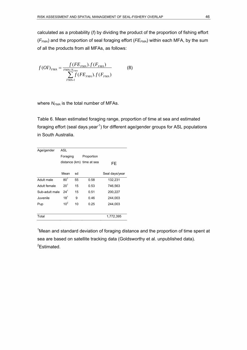
RISK ASSESSMENT AND SPATIAL MANAGEMENT OF SEAL-FISHERY OVERLAP 46
calculated as a probability (f) by dividing the product of the proportion of fishing effort
(FFMA) and the proportion of seal foraging effort (FEFMA) within each MFA, by the sum
of all the products from all MFAs, as follows:
∑=
=
=FMANFMA
FMAFMAFMA
FMAFMAFMA
FfFEf
FfFEfOIf
1)().(
)().()( (8)
where NFMA is the total number of MFAs.
Table 6. Mean estimated foraging range, proportion of time at sea and estimated
foraging effort (seal days.year-1) for different age/gender groups for ASL populations
in South Australia.
Age/gender ASL
Foraging
distance (km) FE
Mean sd
Proportion
time at sea
Seal days/year
Adult male 801 55 0.58 132,231
Adult female 201 15 0.53 746,563
Sub-adult male 241 15 0.51 200,227
Juvenile 181 9 0.46 244,003
Pup 102 10 0.25 244,003
Total 1,772,395
1Mean and standard deviation of foraging distance and the proportion of time spent at
sea are based on satellite tracking data (Goldsworthy et al. unpublished data). 2Estimated.

RISK ASSESSMENT AND SPATIAL MANAGEMENT OF SEAL-FISHERY OVERLAP 47
Table 7. Estimated mean foraging heading (and sd) for adult male ASL based on
satellite tracking studies at several locations in SA (Goldsworthy et al. unpublished
data)
Colony Heading SdNorth Pages Is. 135 90 Seal Slide (Kangaroo Is.) 160 90 Seal Bay (Kangaroo Is.) 180 90 Peaked Rock 180 90 North Is. 180 90 English Is. 190 90 North Neptune, East 190 90 South Neptune, Main 190 90 Dangerous Reef 190 90 Lewis Is. 190 90 Albatross Is. 190 90 Liguanea Is. 200 90 Four Hummocks Is. (north) 200 90 Price Is. 225 90 Rocky (North) Is. 225 90 Pearson Is. 225 90 Ward Is. 225 90 West Waldegrave Is. 225 90 Jones Is. 225 90 Nicolas Baudin Is. 225 90 Olive Is. 225 90 Lilliput Is. 225 90 Blefuscu Is. 225 90 Gliddon Reef 225 90 Breakwater Is. 225 90 Fenelon Is. 225 90 Masillon Is. 225 90 West Is. 225 90 Lounds Is. 225 90 Purdie Is. 225 90 Western Nuyts Reef 200 90 GAB B1 180 90 GAB B2 180 90 GAB B3 180 90 GAB B5 180 90 GAB B6 180 90 GAB B8 180 90 GAB B9 180 90
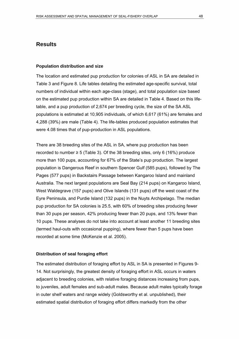
RISK ASSESSMENT AND SPATIAL MANAGEMENT OF SEAL-FISHERY OVERLAP 48
Results
Population distribution and size
The location and estimated pup production for colonies of ASL in SA are detailed in
Table 3 and Figure 8. Life tables detailing the estimated age-specific survival, total
numbers of individual within each age-class (stage), and total population size based
on the estimated pup production within SA are detailed in Table 4. Based on this life-
table, and a pup production of 2,674 per breeding cycle, the size of the SA ASL
populations is estimated at 10,905 individuals, of which 6,617 (61%) are females and
4,288 (39%) are male (Table 4). The life-tables produced population estimates that
were 4.08 times that of pup-production in ASL populations.
There are 38 breeding sites of the ASL in SA, where pup production has been
recorded to number ≥ 5 (Table 3). Of the 38 breeding sites, only 6 (16%) produce
more than 100 pups, accounting for 67% of the State’s pup production. The largest
population is Dangerous Reef in southern Spencer Gulf (585 pups), followed by The
Pages (577 pups) in Backstairs Passage between Kangaroo Island and mainland
Australia. The next largest populations are Seal Bay (214 pups) on Kangaroo Island,
West Waldegrave (157 pups) and Olive Islands (131 pups) off the west coast of the
Eyre Peninsula, and Purdie Island (132 pups) in the Nuyts Archipelago. The median
pup production for SA colonies is 25.5, with 60% of breeding sites producing fewer
than 30 pups per season, 42% producing fewer than 20 pups, and 13% fewer than
10 pups. These analyses do not take into account at least another 11 breeding sites
(termed haul-outs with occasional pupping), where fewer than 5 pups have been
recorded at some time (McKenzie et al. 2005).
Distribution of seal foraging effort
The estimated distribution of foraging effort by ASL in SA is presented in Figures 9-
14. Not surprisingly, the greatest density of foraging effort in ASL occurs in waters
adjacent to breeding colonies, with relative foraging distances increasing from pups,
to juveniles, adult females and sub-adult males. Because adult males typically forage
in outer shelf waters and range widely (Goldsworthy et al. unpublished), their
estimated spatial distribution of foraging effort differs markedly from the other

RISK ASSESSMENT AND SPATIAL MANAGEMENT OF SEAL-FISHERY OVERLAP 49
age/gender groups, because they do not focus their foraging near colonies (Figure
13). The estimated total distribution of foraging effort (age/gender groups combined)
is presented in Figure 14, and demonstrates the greatest concentration of foraging
effort associated with the larger subpopulation centres, especially The Pages (just
east of Kangaroo Island), Seal Bay (south coast of Kangaroo Island), Dangerous
Reef (southern Spencer Gulf) and the Nuyts Archipelago (west Eyre Peninsula). With
the exception of the south-east and northern Gulf waters, some level of ASL foraging
effort occurs in almost all near-coastal waters from Encounter Bay to the West
Australian border (Figure 14).
Distribution of fishing effort
Gill-net sector of the SESSF Data detailing the annual fishing effort (km net-lifts.year-1) for the 29 SA MFAs of the
gill-net sector of the SESSF, spanning 32 years between 1973 and 2004, are
presented in Table 8 and Figure 15A. Over this period, there was a total of 634,496
km of net-lifts, averaging about 20,000 km of net-lifts per year (Table 8, Figure 15A).
Annual effort changed markedly in this region of the fishery, with a steady increase
from around 3,000 km to 12,000 km net-lifts per year between 1973-1983, with a very
significant increase in fishing effort between 1984-1987 peaking at nearly 43,000 km
net-lifts in 1987 (Table 8, Figure 15A). Fishing effort then decreased annually to
about 23,000 km net-lifts in 1993 and then increased to just over 32,000 km net-lifts
in 1998. Fishing effort reduced to around 17,000 km net-lifts in 2000, and has
remained at about this level up until 2004 (Table 8, Figure 15A).
The spatial distribution of fishing effort between 1973 and 2004 is summarised for
four-year averages in Figures 16-23, and total and average annual fishing effort are
present in Figure 24 and 25, respectively. Essentially these track the increase in
fishing effort from the 1970s and the 1980s, with the major regions of fishing effort
occurring south and south-east of Kangaroo Island, and off the west coast of the
Eyre Peninsula (Figures 16-23). Between 2000-2004, about 42% of total fishing effort
occurred south and south east of Kangaroo Island (MFA 149-151, Table 8).
SA Rock lobster fishery (SARLF) Data detailing annual changes in fishing effort over a 35 year period (1970-2004) in
19 MFAs of the SARLF are presented in Table 9 and Figure 15B. Over this period
there was a total of 78.9 million pot-lifts, averaging about 2.3 million pot-lifts/year

RISK ASSESSMENT AND SPATIAL MANAGEMENT OF SEAL-FISHERY OVERLAP 50
(Table 9, Figure 15B). Annual effort in the fishery increased from around 2.2 to 2.5
million pot-lifts per year between the 1970s and 1980s, to a maximum of 2.7 million
pot-lifts in 1991. Since then, fishing effort has decreased and in 2003 and 2004,
averaged just over 1.5 million pot-lifts (Table 9, Figure 15B).
Changes in the spatial distribution of fishing effort in the SARLF between 1970 and
2004 are presented in Figures 26-34. Over this period, about 70% of the total fishing
effort has been concentrated in the south-east of the state in MFAs 55, 56 and 58
(Figures 26-34). Elsewhere, effort is focused close to the shore along the south coast
of Kangaroo Island, and the southern and west coasts of the Eyre Peninsula (Figures
26-34).
Table 8. Annual fishing effort (km net-lifts.year-1) for the 29 SA MFAs of the gill-net
sector of the Commonwealth SESSF, spanning 32 years between 1973 and 2004.
MFA 1973 1974 1975 1976 1977 1978 1979 1980 1981 1982 1983 1984 1985 1986 1987 1988 1989 1990
101 0 0 0 0 0 0 0 0 0 0 108 0 174 0 560 107 741 443
102 0 0 41 0 0 22 16 0 0 80 0 0 0 0 0 14 66 242
103 0 14 2 0 0 0 41 127 79 275 541 48 182 135 504 344 524 524
104 0 0 0 0 0 0 0 0 0 0 0 0 0 120 315 763 482 791
105 0 0 0 0 0 0 0 0 0 0 267 0 0 0 386 279 581 420
106 0 6 0 0 0 0 0 0 72 10 53 15 0 0 256 923 274 989
107 165 279 139 32 108 0 13 287 336 334 810 404 660 1591 2027 1469 821 1593
108 674 746 438 273 626 1029 725 1467 1117 1315 1258 2991 2467 3059 4049 3201 3421 2070
112 0 0 4 0 0 0 0 0 0 0 20 0 0 189 27 444 570 292
113 0 0 6 0 0 0 0 0 0 202 65 74 150 856 524 1200 753 312
114 13 11 2 0 0 0 0 0 96 389 75 461 606 688 1277 2085 1155 1200
115 216 70 156 60 103 35 319 333 524 667 1155 1072 898 1799 1388 1073 2063 582
122 58 75 117 29 106 115 100 276 512 676 413 381 230 229 288 135 42 16
125 0 0 0 0 0 0 0 0 0 0 0 0 0 0 0 0 0 0
126 43 3 1 15 0 20 80 103 830 1045 352 911 1697 1190 1663 2494 2475 2163
128 58 107 0 21 145 284 299 634 888 965 705 1101 870 1035 1108 1095 1579 1094
129 0 0 0 0 206 764 1072 1146 1206 1199 440 419 556 1677 1810 1124 1234 1160
132 52 55 38 14 388 108 181 0 409 478 1209 2782 1260 504 1080 687 853 722
136 78 161 9 0 236 580 165 345 162 122 90 130 38 52 323 372 131 128
138 7 5 43 13 0 0 57 401 345 699 334 1061 923 787 1997 1626 1980 3625
139 57 103 91 92 183 226 233 301 461 1092 558 686 751 1531 3112 1637 2549 1103
140 67 60 74 79 64 445 322 440 519 164 246 462 387 549 1275 1854 2092 1165
144 233 212 415 60 471 471 466 452 417 393 313 303 459 1088 1312 1326 948 1273
148 6 140 0 74 65 84 24 28 51 104 57 345 417 1509 1843 1200 1393 2487
149 124 211 245 93 276 33 0 120 110 183 312 831 965 3417 4620 3975 2425 2871
150 184 236 202 122 40 16 108 274 424 368 694 2093 1388 2991 4329 2327 3120 2568
151 615 233 831 429 805 990 989 1471 996 443 1100 3507 2342 3404 4692 6512 3392 4530
155 313 352 144 183 315 552 1198 328 92 181 123 274 1379 1437 1490 1598 3913 2107
158 165 362 193 344 353 313 288 456 457 220 593 198 187 349 734 488 759 1446
Total 3127 3441 3189 1933 4489 6086 6695 8986 10102 11603 11892 20548 18986 30185 42989 40349 40338 37917
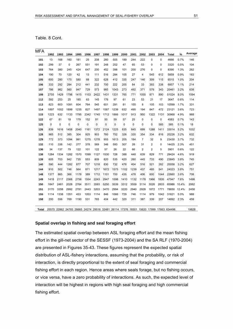
RISK ASSESSMENT AND SPATIAL MANAGEMENT OF SEAL-FISHERY OVERLAP 51
Table. 8 Cont.
Spatial overlap in fishing and seal foraging effort
The estimated spatial overlap between ASL foraging effort and the mean fishing
effort in the gill-net sector of the SESSF (1973-2004) and the SA RLF (1970-2004)
are presented in Figures 35-43. These figures represent the expected spatial
distribution of ASL-fishery interactions, assuming that the probability, or risk of
interaction, is directly proportional to the extent of seal foraging and commercial
fishing effort in each region. Hence areas where seals forage, but no fishing occurs,
or vice versa, have a zero probability of interactions. As such, the expected level of
interaction will be highest in regions with high seal foraging and high commercial
fishing effort.
MFA 1992 1993 1994 1995 1996 1997 1998 1999 2000 2001 2002 2003 2004 Total %
Average
101 13 168 160 181 25 208 280 505 189 244 222 0 0 4666 0.7% 146
102 299 37 0 267 551 191 248 252 47 65 53 0 0 3320 0.5% 104
103 764 380 245 424 647 200 452 398 101 200 276 0 0 8390 1.3% 262
104 190 70 120 42 13 111 516 284 105 27 4 545 612 5859 0.9% 183
105 600 280 175 580 68 322 628 412 335 247 146 309 115 6515 1.0% 204
106 333 292 284 212 441 232 700 222 205 84 33 393 338 6857 1.1% 214
107 786 982 560 947 729 573 985 1043 273 492 371 579 343 20461 3.2% 639
108 2755 1429 1798 1415 1103 2422 1431 1331 765 771 1055 871 890 51024 8.0% 1594
112 592 253 25 185 63 145 176 97 61 23 53 21 17 3647 0.6% 114
113 823 603 1091 604 764 545 601 291 81 155 8 105 103 10599 1.7% 331
114 1897 1002 1899 1235 827 1497 1587 1239 632 495 194 847 472 23121 3.6% 723
115 1223 632 1133 1795 2342 1745 1712 1866 1017 913 950 1322 1131 30968 4.9% 968
122 67 81 18 179 152 81 50 59 57 25 0 0 0 4583 0.7% 143
125 0 0 0 0 0 0 0 0 0 0 0 0 585 585 0.1% 18
126 839 1616 1458 2040 1161 1372 2124 1225 835 645 699 1288 1411 33014 5.2% 1032
128 965 512 385 304 925 903 760 752 326 320 354 334 816 20226 3.2% 632
129 772 373 1094 991 1275 1278 955 1613 205 184 7 32 9 23430 3.7% 732
132 110 338 142 277 378 569 346 593 307 28 31 2 0 14425 2.3% 451
136 34 137 79 122 101 122 57 26 22 66 2 2 5 3901 0.6% 122
138 1284 1334 1282 1570 1099 1127 1530 728 388 448 639 829 771 29424 4.6% 919
139 605 703 942 735 553 809 820 535 420 260 445 733 490 23845 3.8% 745
140 590 444 1282 877 707 1218 830 732 478 404 516 521 282 20058 3.2% 627
144 910 502 746 564 871 1217 1672 1575 1102 1239 437 485 541 24023 3.8% 751
148 1377 865 366 1178 389 1712 1101 700 435 478 406 600 1044 22660 3.6% 708
149 1418 2117 2368 2756 1554 2243 2947 1598 1410 1132 1178 1966 1835 47947 7.6% 1498
150 1847 2461 2028 2764 3511 3593 5250 3539 3312 3559 3114 3026 2833 65986 10.4% 2062
151 3170 3358 2992 2781 2443 3203 3470 2994 3220 2940 2928 1872 1771 78650 12.4% 2458
155 1114 1338 1351 453 1053 1114 846 1066 729 746 1114 979 1042 31621 5.0% 988
158 200 556 769 1190 531 765 404 442 320 311 387 339 207 14692 2.3% 459
Total 25575 22862 24793 26665 24274 29516 32481 26114 17376 16501 15620 17999 17663 634496 19828

RISK ASSESSMENT AND SPATIAL MANAGEMENT OF SEAL-FISHERY OVERLAP 52
Figures 35 and 36, indicate the overlap index (OI) for combined age/gender groups in
the ASL for the SESSF gill-net and SA RLF, respectively. Because fishing effort in
the SESSF gill-net sector occurs in most continental shelf and gulf waters, the OI
highlights that regions where interaction are most likely to occur are closely
associated with the main population centres of ASL, namely, The Pages and Seal
Bay (east and south of Kangaroo Island), Dangerous Reef (southern Spencer Gulf)
and the west coast of the Eyre Peninsula (especially the Nuyts Archipelago) and the
GAB (Figure 35).
This contrasts with the expected spatial interaction with the SARLF. Because most of
the fishing effort in SA RLF is concentrated in the south-east of the State, and in near
coastal waters south and east of Kangaroo Island, and along the southern and west
coasts of the Eyre Peninsula, the OI suggests relatively low interaction rates with The
Pages, and Dangerous Reef ASL subpopulations (Figure 36). However, interactions
with the latter subpopulation occur where their foraging effort intersects fishing effort
in southern Spencer Gulf (Figure 36). As with the SESSF gill-net sector, interactions
rates are expected to be high on the west coast of the Eyre Peninsula, especially in
the Nuyts Archipelago (Figure 36).
Table 9. Annual fishing effort (x1,000’s pot-lifts.year-1) for the 19 Marine Fishing
Areas (MFAs) of the SARLF, spanning 35 years between 1970 and 2004
MFA 1970 1971 1972 1973 1974 1975 1976 1977 1978 1979 1980 1981 1982 1983 1984 1985 1986 1987 19887 5.8 6.2 10.4 11.7 13.0 12.3 12.0 12.5 12.2 9.6 5.9 4.0 6.1 12.6 13.5 5.9 3.7 10.4 7.88 23.5 27.7 24.3 25.7 28.7 51.0 40.9 20.8 21.5 16.4 6.8 1.6 5.2 7.9 15.9 22.9 18.4 5.4 16.110 16.4 18.0 18.4 10.6 12.3 19.7 12.7 13.7 9.8 4.9 0.9 3.6 0.4 3.1 1.8 1.1 0.5 3.2 3.615 32.9 44.6 37.0 51.9 52.2 46.4 52.5 38.7 38.8 49.3 28.8 23.1 25.5 38.4 60.5 43.1 69.2 79.3 74.218 0.0 0.0 0.0 0.8 2.7 0.0 0.0 0.9 3.1 0.0 0.0 2.0 0.0 0.0 0.2 3.2 3.0 3.4 3.127 0.5 3.4 2.1 0.3 3.8 1.5 7.1 5.5 11.9 28.3 32.2 38.2 32.8 43.2 42.7 47.7 45.5 36.6 41.228 76.5 73.2 84.4 70.7 75.8 65.6 66.8 61.3 69.6 57.4 70.9 106.4 97.5 123.0 138.6 135.5 138.8 126.8 119.139 91.6 89.3 97.8 81.4 77.1 70.4 82.2 92.1 107.9 110.7 99.2 94.1 114.3 134.3 121.6 117.4 114.4 159.6 135.240 6.2 8.1 2.8 7.1 14.8 14.7 10.1 31.8 32.3 25.7 43.7 41.8 42.8 47.6 57.8 54.8 53.5 50.0 73.144 0.0 0.0 0.0 0.1 0.3 0.8 0.0 0.3 0.3 0.0 0.5 1.0 0.7 7.5 2.4 2.2 2.8 5.2 3.945 13.6 16.6 19.8 12.7 14.9 14.3 11.4 14.2 13.8 9.5 11.8 14.4 11.0 4.1 2.8 2.5 2.7 4.4 0.546 0.0 0.0 6.7 4.7 0.5 3.2 2.1 1.3 0.4 0.3 0.0 0.0 1.4 0.3 0.0 7.9 3.9 0.0 2.048 12.0 18.8 22.2 15.9 17.2 21.1 14.3 11.9 16.0 27.2 42.9 38.7 50.4 45.8 57.7 45.3 37.6 38.8 70.149 23.2 21.9 44.3 22.7 18.1 16.2 12.4 22.1 20.6 26.4 35.0 44.1 61.7 63.3 51.6 51.8 51.6 47.0 47.150 1.6 4.5 2.0 0.6 0.9 0.1 7.7 3.5 5.9 8.0 2.4 7.3 13.7 42.3 40.9 39.3 38.0 22.4 33.251 219.5 285.3 305.1 279.7 221.1 244.3 225.6 234.2 210.9 203.3 214.6 218.0 238.0 151.5 155.9 141.4 109.2 143.4 121.955 489.2 509.6 600.2 570.3 456.2 517.2 472.6 492.5 487.8 505.6 508.0 612.7 692.3 905.9 793.4 789.0 788.4 809.7 712.356 615.6 663.4 671.6 675.6 567.3 690.7 675.8 683.0 656.7 598.9 744.7 751.3 710.3 609.1 537.6 558.1 509.2 625.9 515.558 499.0 528.6 542.8 591.0 481.2 543.0 484.4 455.5 437.2 481.5 553.4 520.1 509.1 537.8 462.7 481.5 467.7 517.9 503.9
Total 2127 2319 2492 2433 2058 2333 2191 2196 2156 2163 2402 2522 2613 2778 2558 2551 2458 2689 2484

RISK ASSESSMENT AND SPATIAL MANAGEMENT OF SEAL-FISHERY OVERLAP 53
Table 9. Cont.
MFA 1989 1990 1991 1992 1993 1994 1995 1996 1997 1998 1999 2000 2001 2002 2003 2004 Total % Average7 3.7 9.0 7.8 8.6 24.9 17.6 29.1 19.2 14.3 13.7 15.1 17.5 15.6 13.8 12.6 5.2 410 1% 11.48 20.6 18.4 17.8 31.2 38.7 33.9 35.6 32.4 24.7 21.8 24.3 30.2 23.1 19.9 20.9 26.6 809 1% 22.510 1.5 7.1 7.6 5.5 10.9 9.3 9.9 10.9 4.1 6.0 5.1 9.6 9.7 6.3 2.4 2.5 273 0% 29.115 65.1 93.3 103.8 80.6 78.9 69.2 107.3 106.7 86.9 93.8 73.8 72.4 68.3 54.2 43.8 35.4 2135 3% 59.318 2.7 4.1 9.2 7.3 5.9 5.2 9.9 8.3 6.8 9.8 6.1 5.9 5.5 5.7 1.1 1.6 136 0% 16.827 48.4 37.4 38.2 41.7 35.5 38.9 36.2 22.4 29.9 32.4 36.2 22.4 30.9 19.7 24.1 16.5 962 1% 26.728 130.2 108.8 150.6 136.6 118.1 131.9 119.5 139.2 170.0 143.5 110.6 126.9 119.2 110.2 101.9 85.2 3788 5% 105.239 138.1 133.7 143.7 125.5 107.1 117.8 90.4 110.7 115.6 122.0 146.6 116.0 97.8 105.3 107.6 126.6 3934 5% 109.340 72.4 73.0 88.8 78.5 68.8 64.7 76.3 69.5 65.6 66.8 67.4 55.8 41.5 43.8 62.4 67.5 1722 2% 47.844 4.3 3.2 3.6 3.9 3.6 4.4 6.3 5.2 2.7 4.1 6.8 5.7 5.1 8.9 4.5 4.7 1.6 0% 4.145 0.9 1.9 3.1 1.9 0.8 2.9 1.9 1.7 2.0 0.7 0.0 0.2 2.7 1.9 3.4 1.6 267 0% 23.946 4.9 3.2 2.3 6.3 4.1 0.7 0.9 2.5 2.0 2.2 1.6 0.0 0.3 0.0 0.0 1.0 113 0% 10.348 62.9 67.0 78.4 80.3 62.8 48.3 43.3 42.4 46.8 48.9 58.9 50.6 47.5 48.5 53.1 58.7 1551 2% 43.149 60.9 65.5 81.5 70.0 76.9 85.2 80.0 69.4 68.5 67.3 83.9 86.1 90.0 75.2 101.8 67.1 1959 2% 54.450 49.4 17.1 24.2 21.2 30.2 26.7 29.7 26.6 24.6 21.7 20.8 29.5 28.5 18.9 20.9 24.8 689 1% 19.751 124.2 139.1 176.0 119.6 111.5 72.2 73.9 78.0 58.8 45.0 27.2 42.0 21.2 14.8 16.0 18.3 5112 6% 142.055 729.0 803.3 811.2 730.4 683.3 584.2 610.3 656.5 682.8 573.9 437.3 342.4 299.8 276.1 349.0 326.1 20664 26% 574.056 487.4 515.2 561.6 462.8 422.7 442.7 482.8 539.0 552.6 473.4 359.2 333.0 287.6 256.0 322.0 321.6 18936 24% 526.058 407.8 440.4 474.6 431.5 403.9 394.7 410.2 471.4 449.0 429.9 330.5 312.2 284.3 287.2 346.0 370.7 15901 20% 441.7
Total 2414 2541 2784 2443 2289 2150 2254 2412 2408 2177 1811 1658 1479 1366 1593 1562 78865 2253
For ASL, over 60% of the estimated foraging effort occurs in four SESSF gill-net
sector MFAs: MFA 129 (19%, southern Spencer Gulf), MFA 108 (18%, Nuyts
Archipelago), MFA 144 (16%, southern Fleurieu Peninsula) and MFA 149 (8%, south
of Kangaroo Island) (Table 10). Importantly, <1% of the estimated ASL foraging
effort, occurs outside SA MFAs, although at least part of this is in waters to the west
of the SA/WA border, where the SESSF gillnet sector fishery also occurs. Similarly,
over 40% of the estimated ASL foraging effort occurs in four SARL MFAs: MFA 8
(15%, Nuyts Archipelago), MFA 44 (13%, southern Fleurieu Peninsula), MFA 15 (8%,
mid-west coast Eyre Peninsula) and MFA 49 (8%, southern Kangaroo Island).
However, in contrast to the SESSF gill-net sector, 36% of ASL foraging effort occurs
outside of SA RLF MFAs where historical catches have been reported in the SARLF
(Table 10).
Estimated OI between foraging effort in ASL adult females, adult males, sub-adult
males, juveniles and pups with fishing effort in the SESSF gill-net sector and SA RLF
are presented in Figures 37-46. These estimates of spatial overlap indicate that the
probability of interactions is highest close to breeding colonies, where foraging effort
is most focused, especially for pups, juveniles and adult females. Because adult
males do not utilise waters in close proximity to their colonies, the spatial distribution
of OI is relatively dispersed. Because fishing effort in the SARLF has been
RISK ASSESSMENT AND SPATIAL MANAGEMENT OF SEAL-FISHERY OVERLAP 54
concentrated in near coastal waters, the OI is most highly concentrated in ASL pups
and juveniles, especially near breeding colonies (Figures 44 and 46).
Table 10. Average percentage fishing effort among all MFAs in the SESSF gill-net
sector and SARLF, relative to the estimated percentage of foraging effort by different
age/sex classes of ASL within each MFA of each fishery. ‘Outside’ refers to the
percentage of seal foraging effort that occurs outside the listed MFAs.
Gill-net %Fishery ASL % Foraging Effort MFA Effort Females Males SAM Juveniles Pups All ASL
101 0.7 3.2 0.5 3.1 3.6 3.6 2.8 102 0.5 1.9 0.5 1.9 2.0 2.1 1.7 103 1.3 0.4 0.5 0.4 0.4 0.4 0.4 104 0.9 0.3 1.7 0.4 0.0 0.0 0.5 105 1.0 0.1 1.6 0.1 0.0 0.0 0.4 106 1.1 0.2 1.9 0.2 0.2 0.2 0.5 107 3.2 2.4 5.2 2.7 1.5 1.0 2.5 108 8.0 18.5 4.0 17.9 19.9 20.4 16.1 112 0.6 0.0 0.6 0.0 0.0 0.0 0.1 113 1.7 0.0 4.2 0.0 0.0 0.0 0.8 114 3.6 1.7 7.4 1.9 1.2 0.9 2.6 115 4.9 8.1 4.0 7.9 8.4 8.8 7.4 122 0.7 0.0 0.5 0.0 0.0 0.0 0.1 125 0.1 0.1 2.0 0.1 0.0 0.0 0.4 126 5.2 1.0 6.5 1.2 0.7 0.5 2.0 128 3.2 4.6 3.4 4.7 4.2 3.6 4.1 129 3.7 18.4 2.8 17.4 21.4 23.1 16.6 132 2.3 0.1 2.1 0.2 0.0 0.0 0.5 136 0.6 0.0 0.9 0.0 0.0 0.0 0.2 138 4.6 2.8 7.5 3.1 2.0 1.7 3.4 139 3.8 6.1 7.9 6.6 4.5 3.8 5.8 140 3.2 2.3 4.1 2.9 0.6 0.2 2.0 144 3.8 15.5 3.2 14.2 19.7 20.9 14.7 148 3.6 0.7 3.7 0.8 0.2 0.1 1.1 149 7.6 8.4 7.2 8.4 8.5 8.4 8.2 150 10.4 3.1 9.4 3.7 1.0 0.4 3.5 151 12.4 0.0 5.2 0.0 0.0 0.0 1.1 155 5.0 0.0 0.5 0.0 0.0 0.0 0.1 158 2.3 0.0 0.0 0.0 0.0 0.0 0.0
Outside 0.2 1.0 0.2 0.0 0.0 0.3 SARLF MFA
7 0.5 2.4 3.2 2.7 1.5 1.0 1.3 8 1.0 15.3 1.9 14.9 16.3 17.1 16.6 10 0.3 1.3 0.4 1.2 1.7 1.6 1.6 15 2.7 8.1 0.3 7.9 8.4 8.8 8.5 18 0.1 0.3 0.1 0.3 0.1 0.0 0.1 27 1.2 0.4 0.2 0.4 0.5 0.6 0.5 28 4.8 2.6 2.4 2.7 2.4 2.4 2.4 39 4.9 5.8 18.5 6.3 4.3 3.7 4.1 40 2.1 0.6 0.0 0.7 0.2 0.1 0.2 44 0.1 11.4 0.0 9.6 17.2 19.8 18.1 45 0.3 4.0 0.0 4.4 2.5 1.1 2.0 46 0.1 0.0 1.7 0.0 0.0 0.0 0.0 48 1.9 0.7 8.1 0.8 0.2 0.1 0.1 49 2.4 8.4 0.1 8.4 8.5 8.4 8.5 50 0.9 3.1 1.0 3.7 1.0 0.4 0.8 51 6.4 0.0 4.6 0.0 0.0 0.0 0.0 55 26.1 0.0 2.8 0.0 0.0 0.0 0.0 56 23.9 0.0 0.0 0.0 0.0 0.0 0.0 58 20.1 0.0 18.5 0.0 0.0 0.0 0.0
Outside 35.6 43.8 35.8 35.2 35.0 35.1
RISK ASSESSMENT AND SPATIAL MANAGEMENT OF SEAL-FISHERY OVERLAP 55
Population viability analysis
Because of the relative long generation time, subpopulations were classified as
vulnerable (10% probability of quasi-extinction within 100 years) before they were
classified as endangered (20% probability of quasi-extinction in 10 generations; 124
years in ASL). As such, the vulnerable category was superfluous. Further, the critical
and endangered risk categories were grouped because in most simulations,
subpopulations went directly from endangered to quasi-extinct, with no transition
through a critical risk category. As such, population viability analyses delineated
subpopulations as not-threatened, endangered or quasi-extinct, with the endangered
category being inclusive of vulnerable, endangered and critical risk categories.
Results from the population viability analysis for ASL subpopulations based on
results from simulations which assessed the level of additional (ie. anthropogenic)
female pre-recruit mortality (modelled as removals of 0-1.5 year olds per year)
required to place individual subpopulations into different risk categories, with three
population trajectory scenarios (stable r= 0.00, decreasing r =-0.01, and increasing r
=0.05), are presented in Table 11. Results indicate that assuming no additional
female mortalities with the stable and decreasing models developed, 13-27
subpopulations (34-71% of total) respectively, are classed as endangered (20%
probability of extinction within 10 generations, Table 11). Small increases in pre-
recruit female mortality markedly increased the numbers of endangered
subpopulations. An additional mortality of one female per subpopulation/year resulted
in 71% of stable, 84% of decreasing and 5% of increasing subpopulation being
categorised as endangered. Two additional female mortalities per/subpopulation/year
resulted in 84% of stable, 92% of decreasing and 13% of increasing subpopulation
being classed as endangered. The lowest additional mortality level to result in a
subpopulation becoming quasi-extinct was at 0.7 pre-recruit female seals/year (or 1
female per breeding cycle, 1.5 years). At this level of theoretical harvest, 2-5 (5-13%)
subpopulations became quasi-extinct with the stable and decreasing population
models, respectively. Qt times were very short (<2 years, Table 11).
Because of the large number of very small ASL populations, small increases in
additional mortality resulted in increasing numbers of subpopulations reaching the
quasi-extinct threshold. For example, an additional pre-recruit mortality of only two
females/subpopulation/year resulted in 16 subpopulations (42%) becoming quasi-

RISK ASSESSMENT AND SPATIAL MANAGEMENT OF SEAL-FISHERY OVERLAP 56
extinct in the stable model, or 27 (71%) becoming quasi-extinct in the decreasing
model (Table 11, Figure 47). With an additional mortality level of only 3.3 pre-recruit
females/subpopulation/year (5 females/1.5 year stage), 74% of decreasing, 63% of
stable and 11% of increasing subpopulations became quasi-extinct (Table 11, Figure
47). Qt times ranged from as little as 1.5 to 43.1 years in these scenarios. These
population viability simulations suggest that even in the best scenario (populations
increasing at around 5% per/year) many subpopulations are highly vulnerable to
becoming quasi-extinct from low-level additional mortality (Figure 47).
Effects of mortality directed at different stages The above scenarios for ASL demonstrate the susceptibility of subpopulations to
quasi-extinction relative to different rates of female mortality directed at the youngest
age group (0-1.5 years). To investigate how these results may vary in response to
mortalities being directed at other ages/stages, a range of simulated removals of 20
female seals per year was undertaken on a hypothetical population of 1000 female
ASL (slightly larger than the ASL population at Seal Bay, Kangaroo Island) using the
stable population model over 50 reproductive cycles (75 years) (Figure 48). Results
indicate that the highest rate of population reduction is achieved following removal of
females between 3 and 12 years of age, with the greatest impacts achieved from
removal of 4.5-6, 6-7.5 and 7.5-9 age-groups (Figure 48). These are females that are
breeding for their first, second or third times (R. McIntosh pers comm.). In fact the
rate of population decline resulting from mortalities directed at 6-7.5 year olds (-
3.4%/year) was more than three times that of mortalities directed at pups (-
1.1%/year) (Figure 48). Rates of decline were lowest when mortality was directed
towards females older than 18 years of age (Figure 48).
Using the stable (r=0) population model, a comparison was made of the proportion of
subpopulations that reached quasi-extinction under five different scenarios of female
age-groups being subjected to mortality, from ages 0-1.5, 1.5-3, 3-4.5, 4.5-6, and 6-
7.5 (Table 12). Results indicate the increasing vulnerability of subpopulations if
mortality is directed at recruiting-age females. For example, if mortality is directed at
pups, annual mortalities of one female per subpopulation per year result in 5% of
subpopulations becoming quasi-extinct (Table 12). However, when mortalities are
directed at the 6-7.5 year age group, annual mortalities of one female per
subpopulation per year result in 26% of subpopulations becoming quasi-extinct (a
five-fold increase compared to mortality directed at pups) (Table 12). Based on these
estimates, additional mortalities of 1-2 female seals per subpopulation per year could

RISK ASSESSMENT AND SPATIAL MANAGEMENT OF SEAL-FISHERY OVERLAP 57
result in between 5-26% and 42-71% of subpopulations in South Australia becoming
quasi-extinct, respectively, depending on the age of females removed from
subpopulations (Table 12).
Risk classification of subpopulations To examine whether subpopulations could be grouped according to extinction risk, a
Bray-Curtis similarity matrix and hierarchical clustering analysis procedure (Primer
V5.2.2) was undertaken based on PVA outputs using the stable population model
(number of additional female deaths to change status from not threatened to
endangered, endangered to extinct and Qt). This analysis produced four major
groupings, and seven minor groups (Figure 49 and 50). The first major grouping,
termed Very High Risk included 4 subpopulations (11%) (in two subgroups) that were
characterised by fewer than 9 pups, and categorised as endangered in the PVA
analysis with no additional mortality, and had low thresholds of quasi-extinction (0.7-
1.3 additional females/year) and Qt (<10 years). The difference between these two
subpopulations is attributed to slight differences in minimum number of pre-recruit
(aged 0-1.5 years) female deaths/year to bring about extinction (0.7 and 1.3) and Qt
value (Figure 49 and 50).
The next group was termed High Risk, and was the largest group in the analysis with
23 subpopulations (61%). This group contained two subgroups that differed slightly in
risk and Qt. The first subgroup was characterised as having between 9 and 17 pups,
low thresholds of quasi-extinction (≤ 2.0 additional females/year) and moderate Qt
14-26 years). The second subgroup was characterised by larger pup production (21-
43) and slightly greater quasi-extinction threshold (≤ 4.0 additional females/year) and
Qt (<38 years) (Figure 49, Table 11 and 13).
The Moderate Risk group included nine subpopulations (24%), and also contained
two subgroups. The first subgroup was characterised by moderate pup production
(56-84) and extinction thresholds achieved with between 4.7 – 8.7 additional female
deaths/year and Qt times ranging between 39-43 years. The second subgroup was
characterised by producing more than 100 pups (131-214), with quasi-extinction
thresholds between 11.3 – 23.3 additional female deaths/year and Qt times ranging
between 42-47 years (Figure 49, Table 11 and 13).
The Low Risk groups included the two largest subpopulations (Dangerous Reef and
The Pages), which are at least twice the size as any other subpopulation. Quasi-

RISK ASSESSMENT AND SPATIAL MANAGEMENT OF SEAL-FISHERY OVERLAP 58
extinction thresholds and Qt times were relatively high, requiring 50 additional female
deaths/year over a 53-58 year period (Figure 49, Table 11 and 13).
Spatial distribution of subpopulation risk category
There is no clear pattern to the geographical distribution of different risk category
subpopulations, with the four very high risk sites equally spaced along the lower and
western Eyre Peninsula, the Nuyts Archipelago and the Bunda Cliffs (west of the
Head of the Bight). Similarly, high-risk subpopulations are distributed along the same
stretch of coastline, although there is greater density of these subpopulations in the
Bunda Cliffs and lower Eyre Peninsula regions, with one site at Kangaroo Island.
Moderate risk subpopulations are focused in the Nuyts Archipelago and Western
Eyre Peninsula regions (seven sites), with two additional subpopulations in southern
Spencer Gulf and one on Kangaroo Island. The two low risk subpopulations,
Dangerous Reef and The Pages are located in southern Spencer Gulf and east of
Kangaroo Island, respectively. In terms of proximity to particular MFAs within each
fishery, those MFAs in the region of the Bunda Cliffs, the Nuyts Archipelago and
western and lower Eyre Peninsula all contain high and very high risk subpopulations.
Fishery bycatch scenarios
The approach here is to firstly present the expected distribution of bycatch for ASL at
the subpopulation, region and MFA level for both fisheries based on historic
distribution of fishing effort and the expected distribution of seal foraging effort.
Secondly, temporal variation in expected bycatch levels (by region and MFA) are
examined based on historic changes in the distribution of fishing effort in each
fishery. Thirdly, scenarios of different bycatch levels within each fishery are examined
with respect to the historic average distribution of fishing effort to examine the
potential outcomes of different catch rates and how bycatch rates may have varied
among different MFAs. Finally, different scenarios of bycatch level in each fishery are
examined relative to their expected impact on individual subpopulations, in terms of
placing them in different risk categories based on the PVA outputs. These outputs
provide the most coherent presentation of risk-assessment to all subpopulations from
each fishery, and essentially pull together the subpopulation PVAs, the spatial and
temporal overlap in fishing and seal foraging effort in conjunction with different
scenarios of bycatch in each fishery.

RISK ASSESSMENT AND SPATIAL MANAGEMENT OF SEAL-FISHERY OVERLAP 59
Spatial distribution of historic bycatch: gill-net sector SESSF
Based on 32 years (1973-2004) of spatial and temporal variability in fishing effort in
the SESSF gillnet sector, the expected apportioning of bycatch (with a breakdown by
sex) among the different ASL subpopulations is presented in Figure 50. These
analyses indicate that most seals would have been taken from the large populations
of The Pages, Dangerous Reef and Seal Bay, with many of the colonies in the Nuyts
Archipelago and western Eyre Peninsula making up the remainder. From a regional
perspective, The Pages, southern Spencer Gulf (including Dangerous Reef, Peaked
Rocks, North, English, North Neptune (East), South Neptune, Lewis and Albatross
Islands) and the greater Nuyts Archipelago (including Lilliput, Blefuscu, Breakwater,
Fenelon, Masillon, Purdie, and Lounds Islands, Gliddon and Western Nuyts Reef)
make up about 67% of the expected bycatch, followed by Kangaroo Island (Seal Bay
and the Seal Slide)and the Chain of Bays (including Olive, Nicolas Baudin and Jones
islands) (Figure 51A). With respect to the expected breakdown of historical bycatch
in different MFAs, the most prominent is MFA 108 (Nuyts Archipelago), which is
expected to have accounted for more than a quarter of the total historic ASL bycatch
in the fishery (Figure 52). MFAs 149 and 144 (Kangaroo Island and The Pages) and
MFA 129 (southern Spencer Gulf) are expected to have each accounted for about
10% of the overall historic ASL bycatch (Figure 52).
Spatial and temporal distribution of historic bycatch: gill-net sector SESSF
Figures 54, 55, 56 and 57 present the expected breakdown of bycatch per colony
and region, by proportion and number based on historic variability in the amount and
distribution of fishing effort in the SESSF gillnet sector (1973-2004). Due to variability
and the amount and location of fishing effort, the potential impact on ASL in different
regions has changed markedly. The marked increase in fishing effort between the
mid-1980s and 1990s is likely to have resulted in greater levels of bycatch for many
regions (Figure 55, 57). For the most part, the Greater Nuyts and Southern Spencer
Gulf Regions have been the most impacted (in terms of numbers) based on historic
fishing effort data. However, with increased fishing effort in the southeast of SA since
the late 1990s, the relative contribution of The Pages subpopulation to overall
bycatch numbers has likely increased during this period (Figures 54, 56). Predicted
temporal variation in historic bycatch contributions for the six most significant MFAs
(in terms of estimated contribution of ASL bycatch, MFAs 108,115,129, 144, 149 and
150) are presented in Figures 58 and 59. MFA 108 is predicted to have contributed
the highest proportion of ASL bycatch between 1973-2004, even though fishing
RISK ASSESSMENT AND SPATIAL MANAGEMENT OF SEAL-FISHERY OVERLAP 60
effort, and the relative contribution of bycatch in most of the other MFAs increased
throughout the period.
At the end of the historic time series (2004), the proportion and number of seals
expected to have been derived from The Pages, greater Nuyts and southern Spencer
Gulf regions was similar (Figures 54-57). Furthermore, in 2004 MFA 108 is predicted
to have accounted for about 26% of bycatch, with MFA 149, 144 and 129 accounting
for between 11-13%, and MFA 150 and 115 about 7% (Figure 58).
MFA bycatch scenarios: gill-net sector SESSF
Table 14 presents for each gillnet SESSF MFA the average (1973-2004) annual
fishing effort and the proportion of fishing effort and expected ASL bycatch. A range
of possible bycatch scenarios is presented, ranging from and average of 0.0005 to
0.0400 seals per km net-lift/year. Average bycatch rates are calculated by dividing
the number of seals caught by the total fishing effort in those MFAs where seals
where caught. Based on the ASL foraging effort models, the only MFA in SA where
ASL are not expected to become bycatch is in MFA 158. At a bycatch rate of 0.0005
seals/km lift/year (approximately 10 seals, ie.1 seal/2,000km net-lift), the bycatch
rates among MFAs ranges from 0 to 0.08 (Table 14). At an average bycatch rate of
0.04 seals/km-lift/year (775 seals, ie. 1 seal/25km net-lift), the MFA bycatch rates
vary from 0 to 0.128 (Table 14). In all bycatch scenarios, the proportion of bycatch
apportioned to each MFA is the same.
Subpopulation PVA with bycatch scenarios: gill-net sector SESSF
Figure 60 indicates the overall bycatch number and average rate required to place
different ASL subpopulations into different risk categories. These are based on the
number of female mortalities attributed to individual subpopulations, as determined
by the overlap in estimated foraging effort and the average (1973-2004) distribution
of fishing effort (see Table 14). The bycatch number refers to the total number seals
caught per year, of which about 52% are female that are apportioned out among the
38 subpopulations. The estimated number of additional female mortalities per year
required to place subpopulations into the various risk categories (based on PVA
using the stable population model, see Table 11) was combined with the bycatch
scenario analysis to provide an integrated risk assessment analyses. The PVA
indicates which subpopulations can least afford to lose individuals, but it does not

RISK ASSESSMENT AND SPATIAL MANAGEMENT OF SEAL-FISHERY OVERLAP 61
indicate whether those subpopulations are likely to lose individual seals based on the
distribution of seal foraging and fishing effort. Figure 60 integrates the spatial bycatch
analysis with the PVA approach, and therefore identifies which subpopulation should
be classified as most at risk under different bycatch scenarios.
With no additional bycatch mortalities, 24% of ASL subpopulations in South
Australian are categorised as endangered. However, if bycatch mortality in the
demersal shark fishery was 50, 100, 150 and 200 seals per year, the percentage of
endangered subpopulations would increase to 45%, 68%, 84% and 92%,
respectively (Figure 60). These results highlight just how vulnerable subpopulations
are to small increases in additional mortality. The ten most at risk subpopulations
(risk of quasi-extinction from bycatch mortality) in the demersal shark fishery, occur in
the Nuyts Archipelago and Kangaroo Island regions. Seven subpopulations occur
within the Nuyts Archipelago, all within demersal gillnet marine fishing area (MFA)
108 (Olive, Lilliput, West, Purdie, Blefuscu, and Lounds Island and Breakwater Reef).
Based on population viability analyses, subpopulation foraging models and fishery
interaction probabilities, these seven subpopulations would become quasi-extinct if
total annual bycatch levels in the whole gillnet fishery were between 262 and 346
seals (Figure 60). For individual subpopulations this equated to as little as between
two (Breakwater Reef) and 12 (Purdie Island) female bycatch mortalities per year
(Table 11). The next three most vulnerable subpopulations were in the Kangaroo
Island region (Seal Bay, Seal Slide and The Pages), which were estimated to
become quasi-extinct when total annual bycatch in the fishery reached between 349
and 392 seals (Figure 60). For these three subpopulations, this equated to between
1.3 (Seal Slide) and 50 (The Pages) female bycatch mortalities per year (Table 11).

RISK ASSESSMENT AND SPATIAL MANAGEMENT OF SEAL-FISHERY OVERLAP 62
Table 11. Summary of population viability analysis (PVA) for ASL subpopulations in
South Australia. The table presents results from simulations assessing the level of
additional female pre-recruit mortality (modelled as annual removal of 1.5 year olds)
required to place individual subpopulations into different risk categories (E+C=
endangered and critical, Extinct = quasi-extinct), based on the three population
trajectory scenarios (stable r= 0.00, decreasing r =-0.01, and increasing r =0.05). Qt
represents quasi-extinction time (years). The estimated pup production of each
subpopulation is given (see Table 3) and subpopulations are ranked according to
risk.
Amount of annual additional pre-recruit female mortality to change subpopulation risk
Subpopulation Pup Decreasing
λ= 0.9801, r=-0.01 Stable λ =1, r=0
Increasing λ = 1.0985, r=0.05
No. E+C Extinct Qt E+C Extinct Qt E+C Extinct Qt
GAB B2 5 0.0 0.7 1.5 0.0 0.7 1.7 0.7 2.7 1.8 South Neptune Is. 6 0.0 0.7 1.5 0.0 0.7 1.8 0.7 2.7 1.8 Gliddon Reef 7 0.0 0.7 9.9 0.0 1.3 7.5 1.3 3.3 10.5 Ward Is. 8 0.0 0.7 9.9 0.0 1.3 9.5 1.3 3.3 10.5 Masillon Is. 9 0.0 0.7 16.8 0.0 1.3 14.6 2.0 4.0 17.0 Seal Slide 11 0.0 1.3 15.2 0.0 1.3 19.2 2.7 4.7 17.0 Four Hummocks Is. 12 0.0 1.3 15.2 0.0 2.0 15.8 2.7 4.7 17.0 GAB B6 12 0.0 1.3 15.2 0.0 1.3 19.2 2.7 4.7 17.0 North Neptune (East) Is. 14 0.0 1.3 20.3 0.0 2.0 19.2 3.3 5.3 19.4 Western Nuyts Reef 14 0.0 1.3 20.3 0.0 2.0 19.2 3.3 6.0 19.5 Albatross Is. 15 0.0 1.3 22.8 0.0 2.0 21.8 3.3 6.7 12.5 Jones Is. 15 0.0 1.3 22.8 0.0 2.0 21.8 3.3 6.7 18.8 GAB B1 15 0.0 1.3 22.8 0.0 2.0 21.8 3.3 6.7 18.8 Rocky (North) Is. 16 0.0 1.3 22.8 0.1 2.0 23.7 3.3 6.7 18.8 GAB B9 17 0.0 2.0 21.3 0.1 2.0 25.1 4.0 7.3 21.0 Breakwater Reef 17 0.0 2.0 21.3 0.1 2.0 25.7 3.3 6.0 20.6 Fenelon Is. 21 0.0 1.3 33.9 0.2 2.7 25.1 4.7 8.7 22.8 Peaked Rock 24 0.0 1.3 36.2 0.4 2.7 30.3 5.3 8.7 23.3 Price Is. 25 0.0 2.0 28.5 0.3 2.7 30.3 5.3 10.0 23.3 Lounds Is. 26 0.0 2.0 28.5 0.3 2.7 31.2 5.3 10.0 23.4 Pearson Is. 27 0.0 2.0 33.9 0.4 3.3 30.0 6.0 10.0 26.6 English Is. 27 0.0 2.0 34.2 0.4 3.3 29.7 5.3 10.0 24.0 North Is. 28 0.0 2.0 34.2 0.4 3.3 29.7 5.3 10.0 24.0 GAB B3 31 0.0 2.0 36.6 0.5 3.3 32.3 6.7 11.3 25.4 GAB B8 38 0.0 2.0 39.6 1.0 4.0 34.8 8.0 13.3 28.1 Liguanea Is. 43 0.0 2.0 45.9 1.0 4.0 37.2 9.3 16.0 26.1
GAB B5 43 0.0 2.0 45.9 1.0 4.0 37.2 8.7 15.3 27.0
West Is. 56 0.3 3.3 43.1 1.3 4.7 42.8 11.3 23.3 25.1
Lilliput Is. 67 0.3 4.0 45.3 1.3 6.0 41.9 14.0 23.3 31.7
Nicolas Baudin Is. 72 0.0 4.0 47.3 2.0 7.3 39.3 14.7 26.7 0.0
Lewis Is. 73 0.3 4.0 46.7 2.0 7.3 40.5 14.0 24.7 32.4
Blefuscu Is. 84 0.4 5.3 44.1 2.0 8.7 39.3 20.0 30.0 30.6
Olive Is. 131 1.3 6.0 55.7 3.3 11.3 46.5 26.7 43.3 34.8
Purdie Is. 132 1.3 6.7 52.5 3.3 12.0 45.0 26.0 45.3 33.0
West Waldegrave Is. 157 2.0 8.0 52.8 4.0 14.0 45.6 33.3 53.3 33.8 Seal Bay 214 2.7 10.0 59.6 5.3 21.3 44.9 42.0 72.7 34.1 The Pages 577 6.7 27.3 62.7 16.7 50.7 53.9 120.0 183.3 39.2 Dangerous Reef 585 6.7 28.0 60.3 16.7 48.7 55.1 117.3 190.0 38.1

RISK ASSESSMENT AND SPATIAL MANAGEMENT OF SEAL-FISHERY OVERLAP 63
Table 12. Comparison of the proportion of subpopulations of ASL reaching quasi-
extinction subject to increasing additional female mortality, under five scenarios of
different age-groups subjected to mortality. The age-groups are 0-1.5, 1.5-3, 3-4.5,
4.5-6, and 6-7.5 years. Calculations are based on the stable population model (r=0).
Percentage of subpopulations that become quasi-extinct relative to age-group from which additional females are removed
Stages/Age-group
Number of additional female
deaths/ subpopulation/year
0.-1.5 1.5-3 3-4.5 4.5-6 6-7.5
0.10 0 0 0 0 0
0.22 0 0 0 0 0
0.33 0 0 0 0 0
0.44 0 0 0 0 0
0.50 0 0 0 0 0
0.67 5 13 13 21 26
1.00 5 13 16 26 26
1.33 5 13 16 26 26
2.00 42 63 71 71 71
2.7 53 71 74 74 79
3.3 53 71 74 74 79
4.0 71 82 84 84 84
4.7 74 84 84 84 89
5.3 74 84 84 84 89
6.0 76 84 89 89 89
6.7 76 84 89 92 92
7.3 76 84 89 92 92
8.0 82 89 92 92 92
8.7 84 92 92 92 95
9.3 84 92 92 92 95
10.0 84 92 92 95 95
10.7 84 92 95 95 95
11.3 84 92 95 95 95
12.0 89 95 95 95 95
12.7 89 95 95 95 95
13.3 89 95 95 95 95
14.0 92 95 95 95 95
16.7 92 95 95 95 95
20.0 92 95 95 95 95
23.3 92 95 95 95 100
26.7 95 95 100 100 100
30.0 95 97 100 100 100
33.3 95 97 100 100 100
36.7 95 100 100 100 100
40.0 95 100 100 100 100
43.3 95 100 100 100 100
46.7 97 100 100 100 100
50.0 100 100 100 100 100

RISK ASSESSMENT AND SPATIAL MANAGEMENT OF SEAL-FISHERY OVERLAP 64
Table 13. Summary of PVA outcomes for SA ASL subpopulations, grouped in risk
categories.
Additional female mortalities to change subpopulation status
Risk Category
Group
No. pups
No. subpops
Endangered/critical
Extinct
Qt (years)
Very High Risk (11%) 1 5-6 2 0.0 0.7 1.7-1.8 2 7-8 2 0.0 1.3 7.5-9.5 High Risk (61%) 3 9-17 12 0.0-0.1 1.3-2 14.6-25.7 4 21-43 11 0.2-1.0 2.7-4 25.1-37.2 Moderate Risk (24%) 5 56-84 5 1.3-2.0 4.7-8.7 39.3-42-8 6 131-214 4 3.3-5.3 11.3-21.3 42-46.5 Low Risk (5%) 7 577-585 2 16.7 18.7-50.9 53.6-57.5
Spatial distribution of historic bycatch: SA Rock lobster fishery
Based on 35 years (1970-2004) of spatial and temporal variability in fishing effort in
the SA RLF, the estimated apportioning of bycatch among the different ASL
subpopulations is presented in Figure 50. This analysis suggest that in terms of
numbers, most bycatch seals would have been taken from Seal Bay (20%) and West
Waldegrave Island (16%) (Figure 50). Many of the subpopulations in the southern
Spencer Gulf region, including Dangerous Reef, Lewis, Liguanea and Price Islands
were also likely to have contributed significantly to bycatch in the SA RLF (Figure
50). These southern Spencer Gulf subpopulations likely contributed to most of the
bycatch (24%), followed by Kangaroo Island (21%), Western Eyre Peninsula (195)
and the Greater Nuyts Archipelago (13%, Figure 51B).
With respect to the estimated spread of historical bycatch across different MFAs, five
MFAs would have accounted for most (94%) of it (Figure 53. The main ones being
MFA 15 (24%), MFA 39 (20%) and MFA 49 (21%), followed by MFA 8 (17%) and
MFA 28 (12%) (Figure 53).
Spatial and temporal distribution of historic bycatch: SA Rock lobster fishery
Figures 56 and 57 present the expected breakdown of bycatch per region by
proportion and number based on historic variability in the amount and distribution of
fishing effort in the SA RLF (1970-2004). The proportion and number of seals taken
from the different regions are likely to have varied considerably over this period, with
a general increase in the importance of Kangaroo Island, especially since the late
1990s (Figures 56 and 57). Southern Spencer Gulf and the western Eyre regions are
RISK ASSESSMENT AND SPATIAL MANAGEMENT OF SEAL-FISHERY OVERLAP 65
also likely to have been significant in their contribution to bycatch, and to a lesser
extent, the Greater Nuyts Archipelago (Figures 56 and 57).
Predicted temporal variation in historical bycatch contributions from the five most
significant MFAs (MFAs 49, 39, 28, 15, and 8), is presented in Figures 7.27a and
7.28a. There is a clear trend for increasing bycatch contribution (both percentage and
number) from MFA 49, especially since the late 1990s, when the contribution from
MFA 15 began to decline markedly.
MFA bycatch scenarios: SA Rock lobster fishery
Table 15 presents the average (1970-2004) annual fishing effort per SA RLF MFA,
and the proportion of fishing effort and expected ASL bycatch for each MFA. A range
of possible bycatch scenarios is presented, ranging from an average of 0.005 to
0.500 seals/1,000 pot-lifts/year. Average bycatch rates were calculated by dividing
the number of seals caught by the total fishing effort in those MFAs where seals
where caught. Based on the ASL foraging effort models and these bycatch
scenarios, there are five MFAs in SA where ASL are not expected to become
bycatch. These are MFA 46, 51, 55, 56 and 58 (Table 15). At a bycatch rate of 0.005
seals/1,000 pot-lifts/year (ie.1 seal/200,000 pot-lifts), the bycatch rates among MFAs
ranges from 0 to 0.02 seals/1,000 pot-lifts (Table 15). At an average bycatch rate of
0.500 seals/1,000 pot-lifts/year (ie. 1 seal/2,000 pot-lifts), the MFA bycatch rates vary
from 0 to 2.2 seals/1,000 pot-lifts (Table 15).
Subpopulation PVA with bycatch scenarios
If bycatch mortality in the southern rock lobster fishery was 50, 100, 150 and 200
ASL per year (Figure 60), then the percentage of subpopulations in South Australian
categorised as endangered would increase from 24% (zero bycatch) to 53%, 66%,
79% and 82%, respectively. The ten ASL subpopulations at greatest risk of extinction
to bycatch in the South Australian southern rock lobster fishery included Price Island,
Peaked Rocks, South and North Neptune Islands, North and Liguanea Islands in the
southern Spencer Gulf/lower Eyre Peninsula region, West Waldegrave and Jones
Island (west Eyre Peninsula) and Seal Bay and the Seal Slide (Kangaroo Island)
(Figure 60). Based on population viability analyses, subpopulation foraging models
and fishery interaction probabilities, the most at-risk subpopulations would become
extinct if total annual bycatch levels in the fishery reached between 127 and 254

RISK ASSESSMENT AND SPATIAL MANAGEMENT OF SEAL-FISHERY OVERLAP 66
seals (Figure 60). For individual subpopulations, this equated to as little as between
0.7 (South Neptune Island) and 23 (Seal Bay) female bycatch mortalities per year.
Table 14. Hypothetical ASL bycatch scenarios in the gillnet sector of the SESSF off
SA. Average (1973-2004) annual fishing effort per MFA, the proportion of fishing
effort and expected proportion of ASL bycatch per MFA are presented with a range of
possible bycatch scenarios, ranging from an average of 0.0005 to 0.0400 seals per
km net-lift/year. Individual MFA bycatch rates are given for each scenario.
Average bycatch rate gillnet SESSF (seals/km net-lift)
Gillnet SESSF 0.0005 0.0010 0.0020 0.0030 0.0040 0.0050 0.006
MFA
Fishing effort
(km lifts)
Prop. fishing effort
Prop. seal
bycatch
No.
MFA bycatch
rate No.
MFA bycatch
rate No.
MFA bycatch
rate No.
MFA bycatch
rate No.
MFA bycatch
rate No.
MFA bycatch
rate No.
MFA bycatch
rate
101 146 0.007 0.004 0.0 0.0003 0.1 0.0006 0.2 0.0011 0.2 0.0017 0.3 0.0022 0.4 0.0028 0.5 0.0033
102 104 0.005 0.002 0.0 0.0002 0.0 0.0003 0.1 0.0007 0.1 0.0010 0.1 0.0013 0.2 0.0017 0.2 0.0020
103 262 0.013 0.001 0.0 0.0000 0.0 0.0001 0.0 0.0002 0.1 0.0002 0.1 0.0003 0.1 0.0004 0.1 0.0005
104 183 0.009 0.001 0.0 0.0000 0.0 0.0001 0.0 0.0002 0.1 0.0003 0.1 0.0004 0.1 0.0005 0.1 0.0006
105 204 0.010 0.001 0.0 0.0000 0.0 0.0001 0.0 0.0001 0.0 0.0002 0.1 0.0003 0.1 0.0004 0.1 0.0004
106 214 0.011 0.001 0.0 0.0001 0.0 0.0001 0.0 0.0002 0.1 0.0003 0.1 0.0004 0.1 0.0005 0.1 0.0006
107 639 0.032 0.017 0.2 0.0003 0.3 0.0005 0.6 0.0010 1.0 0.0015 1.3 0.0020 1.6 0.0025 1.9 0.0030
108 1594 0.080 0.264 2.6 0.0016 5.1 0.0032 10.2 0.0064 15.3 0.0096 20.5 0.0128 25.6 0.0160 30.7 0.0192
112 114 0.006 0.000 0.0 0.0000 0.0 0.0000 0.0 0.0000 0.0 0.0001 0.0 0.0001 0.0 0.0001 0.0 0.0001
113 331 0.017 0.003 0.0 0.0001 0.1 0.0002 0.1 0.0003 0.2 0.0005 0.2 0.0007 0.3 0.0008 0.3 0.0010
114 723 0.036 0.019 0.2 0.0003 0.4 0.0005 0.7 0.0010 1.1 0.0016 1.5 0.0021 1.9 0.0026 2.2 0.0031
115 968 0.049 0.074 0.7 0.0007 1.4 0.0015 2.9 0.0030 4.3 0.0044 5.7 0.0059 7.2 0.0074 8.6 0.0089
122 143 0.007 0.000 0.0 0.0000 0.0 0.0000 0.0 0.0000 0.0 0.0001 0.0 0.0001 0.0 0.0001 0.0 0.0001
125 18 0.001 0.000 0.0 0.0000 0.0 0.0001 0.0 0.0002 0.0 0.0003 0.0 0.0003 0.0 0.0004 0.0 0.0005
126 1032 0.052 0.021 0.2 0.0002 0.4 0.0004 0.8 0.0008 1.2 0.0012 1.6 0.0016 2.0 0.0020 2.4 0.0024
128 632 0.032 0.026 0.3 0.0004 0.5 0.0008 1.0 0.0016 1.5 0.0024 2.0 0.0032 2.6 0.0040 3.1 0.0049
129 732 0.037 0.125 1.2 0.0017 2.4 0.0033 4.8 0.0066 7.3 0.0099 9.7 0.0132 12.1 0.0165 14.5 0.0198
132 451 0.023 0.002 0.0 0.0000 0.0 0.0001 0.1 0.0002 0.1 0.0003 0.2 0.0004 0.2 0.0005 0.3 0.0006
136 122 0.006 0.000 0.0 0.0000 0.0 0.0000 0.0 0.0001 0.0 0.0001 0.0 0.0001 0.0 0.0002 0.0 0.0002
138 919 0.046 0.032 0.3 0.0003 0.6 0.0007 1.2 0.0014 1.9 0.0020 2.5 0.0027 3.1 0.0034 3.7 0.0041
139 745 0.038 0.044 0.4 0.0006 0.9 0.0011 1.7 0.0023 2.6 0.0034 3.4 0.0046 4.3 0.0057 5.1 0.0069
140 627 0.032 0.013 0.1 0.0002 0.3 0.0004 0.5 0.0008 0.8 0.0012 1.0 0.0016 1.3 0.0020 1.5 0.0024
144 751 0.038 0.113 1.1 0.0015 2.2 0.0029 4.4 0.0058 6.6 0.0088 8.8 0.0117 11.0 0.0146 13.1 0.0175
148 708 0.036 0.008 0.1 0.0001 0.2 0.0002 0.3 0.0004 0.5 0.0007 0.6 0.0009 0.8 0.0011 0.9 0.0013
149 1498 0.076 0.126 1.2 0.0008 2.4 0.0016 4.9 0.0033 7.3 0.0049 9.8 0.0065 12.2 0.0081 14.6 0.0098
150 2062 0.104 0.074 0.7 0.0003 1.4 0.0007 2.9 0.0014 4.3 0.0021 5.8 0.0028 7.2 0.0035 8.7 0.0042
151 2458 0.124 0.027 0.3 0.0001 0.5 0.0002 1.0 0.0004 1.5 0.0006 2.1 0.0008 2.6 0.0010 3.1 0.0013
155 988 0.050 0.001 0.0 0.0000 0.0 0.0000 0.0 0.0000 0.1 0.0001 0.1 0.0001 0.1 0.0001 0.1 0.0001
158 459 0.020 0.000 0.0 0.0000 0.0 0.0000 0.0 0.0000 0.0 0.0000 0.0 0.0000 0.0 0.0000 0.0 0.0000
Sum 19,828 Total seals 10 19 39 58 77 97 116
Continued on next page.
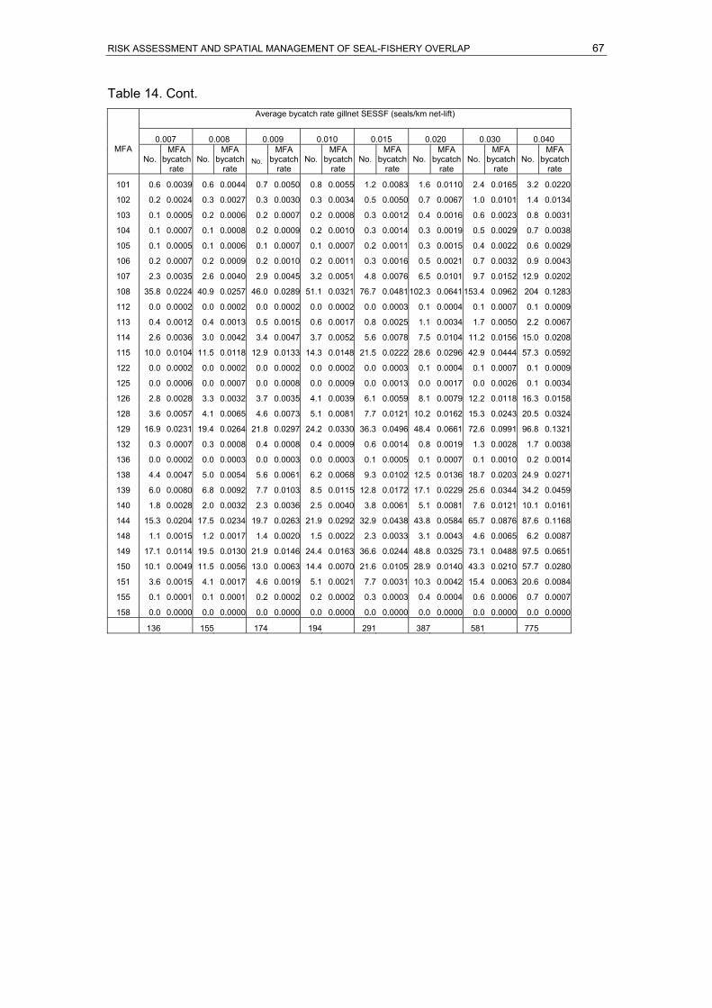
RISK ASSESSMENT AND SPATIAL MANAGEMENT OF SEAL-FISHERY OVERLAP 67
Table 14. Cont. Average bycatch rate gillnet SESSF (seals/km net-lift)
0.007 0.008 0.009 0.010 0.015 0.020 0.030 0.040 MFA
No.
MFA bycatch
rate No.
MFA bycatch
rate No.
MFA bycatch
rate No.
MFA bycatch
rate No.
MFA bycatch
rate No.
MFA bycatch
rate No.
MFA bycatch
rate No.
MFA bycatch
rate
101 0.6 0.0039 0.6 0.0044 0.7 0.0050 0.8 0.0055 1.2 0.0083 1.6 0.0110 2.4 0.0165 3.2 0.0220
102 0.2 0.0024 0.3 0.0027 0.3 0.0030 0.3 0.0034 0.5 0.0050 0.7 0.0067 1.0 0.0101 1.4 0.0134
103 0.1 0.0005 0.2 0.0006 0.2 0.0007 0.2 0.0008 0.3 0.0012 0.4 0.0016 0.6 0.0023 0.8 0.0031
104 0.1 0.0007 0.1 0.0008 0.2 0.0009 0.2 0.0010 0.3 0.0014 0.3 0.0019 0.5 0.0029 0.7 0.0038
105 0.1 0.0005 0.1 0.0006 0.1 0.0007 0.1 0.0007 0.2 0.0011 0.3 0.0015 0.4 0.0022 0.6 0.0029
106 0.2 0.0007 0.2 0.0009 0.2 0.0010 0.2 0.0011 0.3 0.0016 0.5 0.0021 0.7 0.0032 0.9 0.0043
107 2.3 0.0035 2.6 0.0040 2.9 0.0045 3.2 0.0051 4.8 0.0076 6.5 0.0101 9.7 0.0152 12.9 0.0202
108 35.8 0.0224 40.9 0.0257 46.0 0.0289 51.1 0.0321 76.7 0.0481102.3 0.0641153.4 0.0962 204 0.1283
112 0.0 0.0002 0.0 0.0002 0.0 0.0002 0.0 0.0002 0.0 0.0003 0.1 0.0004 0.1 0.0007 0.1 0.0009
113 0.4 0.0012 0.4 0.0013 0.5 0.0015 0.6 0.0017 0.8 0.0025 1.1 0.0034 1.7 0.0050 2.2 0.0067
114 2.6 0.0036 3.0 0.0042 3.4 0.0047 3.7 0.0052 5.6 0.0078 7.5 0.0104 11.2 0.0156 15.0 0.0208
115 10.0 0.0104 11.5 0.0118 12.9 0.0133 14.3 0.0148 21.5 0.0222 28.6 0.0296 42.9 0.0444 57.3 0.0592
122 0.0 0.0002 0.0 0.0002 0.0 0.0002 0.0 0.0002 0.0 0.0003 0.1 0.0004 0.1 0.0007 0.1 0.0009
125 0.0 0.0006 0.0 0.0007 0.0 0.0008 0.0 0.0009 0.0 0.0013 0.0 0.0017 0.0 0.0026 0.1 0.0034
126 2.8 0.0028 3.3 0.0032 3.7 0.0035 4.1 0.0039 6.1 0.0059 8.1 0.0079 12.2 0.0118 16.3 0.0158
128 3.6 0.0057 4.1 0.0065 4.6 0.0073 5.1 0.0081 7.7 0.0121 10.2 0.0162 15.3 0.0243 20.5 0.0324
129 16.9 0.0231 19.4 0.0264 21.8 0.0297 24.2 0.0330 36.3 0.0496 48.4 0.0661 72.6 0.0991 96.8 0.1321
132 0.3 0.0007 0.3 0.0008 0.4 0.0008 0.4 0.0009 0.6 0.0014 0.8 0.0019 1.3 0.0028 1.7 0.0038
136 0.0 0.0002 0.0 0.0003 0.0 0.0003 0.0 0.0003 0.1 0.0005 0.1 0.0007 0.1 0.0010 0.2 0.0014
138 4.4 0.0047 5.0 0.0054 5.6 0.0061 6.2 0.0068 9.3 0.0102 12.5 0.0136 18.7 0.0203 24.9 0.0271
139 6.0 0.0080 6.8 0.0092 7.7 0.0103 8.5 0.0115 12.8 0.0172 17.1 0.0229 25.6 0.0344 34.2 0.0459
140 1.8 0.0028 2.0 0.0032 2.3 0.0036 2.5 0.0040 3.8 0.0061 5.1 0.0081 7.6 0.0121 10.1 0.0161
144 15.3 0.0204 17.5 0.0234 19.7 0.0263 21.9 0.0292 32.9 0.0438 43.8 0.0584 65.7 0.0876 87.6 0.1168
148 1.1 0.0015 1.2 0.0017 1.4 0.0020 1.5 0.0022 2.3 0.0033 3.1 0.0043 4.6 0.0065 6.2 0.0087
149 17.1 0.0114 19.5 0.0130 21.9 0.0146 24.4 0.0163 36.6 0.0244 48.8 0.0325 73.1 0.0488 97.5 0.0651
150 10.1 0.0049 11.5 0.0056 13.0 0.0063 14.4 0.0070 21.6 0.0105 28.9 0.0140 43.3 0.0210 57.7 0.0280
151 3.6 0.0015 4.1 0.0017 4.6 0.0019 5.1 0.0021 7.7 0.0031 10.3 0.0042 15.4 0.0063 20.6 0.0084
155 0.1 0.0001 0.1 0.0001 0.2 0.0002 0.2 0.0002 0.3 0.0003 0.4 0.0004 0.6 0.0006 0.7 0.0007
158 0.0 0.0000 0.0 0.0000 0.0 0.0000 0.0 0.0000 0.0 0.0000 0.0 0.0000 0.0 0.0000 0.0 0.0000
136 155 174 194 291 387 581 775

RISK ASSESSMENT AND SPATIAL MANAGEMENT OF SEAL-FISHERY OVERLAP 68 68
Table 15. Hypothetical ASL bycatch scenarios in the SA RLF. Average (1970-2004) annual fishing effort per MFA, the proportion of fishing effort and expected proportion of
ASL bycatch per MFA are presented. A range of possible bycatch scenarios is presented, ranging from an average of 0.005 to 0.500 seals per 1,000 pot-lifts/year and
bycatch rates are given for each scenario.
Average bycatch rate SA Rock Lobster Fishery (seals/1,000 pot-lift) SA Rock Lobster
0.005 0.010 0.020 0.030 0.040 0.050 0.06 0.070 0.080 0.090 0.100 0.200 0.300 0.400 0.500
MFA
Fishing effort (1,000 lifts)
Prop. fishing effort
Prop. seal
bycatch
No.
MFA bycatch
rate No.
MFA bycatch
rate No.
MFA bycatch
rate No.
MFA bycatch
rate No.
MFA bycatch
rate No.
MFA bycatch
rate No.
MFA bycatch
rate No.
MFA bycatch
rate No.
MFA bycatch
rate No.
MFA bycatch
rate No.
MFA bycatch rate
No.
MFA bycatch
rate No.
MFA bycatch
rate No.
MFA bycatch
rate No.
MFA bycatch
rate
7 11.5 0.005 0.006 0.0 0.0015 0.0 0.0029 0.1 0.0058 0.1 0.0087 0.1 0.0117 0.2 0.0146 0.2 0.0175 0.2 0.0204 0.3 0.0233 0.3 0.0262 0.3 0.0291 0.7 0.0583 1.0 0.0874 1.3 0.1165 1.7 0.1457
8 22.9 0.010 0.1732 0.5 0.0199 0.9 0.0398 1.8 0.0796 2.7 0.1194 3.6 0.1592 4.6 0.1990 5.5 0.2388 6.4 0.2786 7.3 0.3184 8.2 0.3581 9.1 0.3979 18.2 0.7959 27.3 1.1938 36.4 1.5918 45.5 1.9897
10 7.5 0.003 0.0055 0.0 0.0019 0.0 0.0039 0.1 0.0078 0.1 0.0116 0.1 0.0155 0.1 0.0194 0.2 0.0233 0.2 0.0272 0.2 0.0310 0.3 0.0349 0.3 0.0388 0.6 0.0776 0.9 0.1164 1.2 0.1552 1.5 0.1940
15 60.6 0.027 0.2362 0.6 0.0103 1.2 0.0205 2.5 0.0410 3.7 0.0615 5.0 0.0820 6.2 0.1026 7.5 0.1231 8.7 0.1436 9.9 0.1641 11.2 0.1846 12.4 0.2051 24.8 0.4102 37.3 0.6154 49.7 0.8205 62.1 1.0256
18 3.4 0.001 0.0001 0.0 0.0001 0.0 0.0001 0.0 0.0003 0.0 0.0004 0.0 0.0005 0.0 0.0007 0.0 0.0008 0.0 0.0009 0.0 0.0010 0.0 0.0012 0.0 0.0013 0.0 0.0026 0.0 0.0039 0.0 0.0052 0.0 0.0065
27 26.7 0.012 0.0065 0.0 0.0006 0.0 0.0013 0.1 0.0026 0.1 0.0038 0.1 0.0051 0.2 0.0064 0.2 0.0077 0.2 0.0089 0.3 0.0102 0.3 0.0115 0.3 0.0128 0.7 0.0256 1.0 0.0383 1.4 0.0511 1.7 0.0639
28 107.4 0.048 0.1172 0.3 0.0029 0.6 0.0057 1.2 0.0115 1.8 0.0172 2.5 0.0229 3.1 0.0287 3.7 0.0344 4.3 0.0401 4.9 0.0459 5.5 0.0516 6.2 0.0574 12.3 0.1147 18.5 0.1721 24.6 0.2294 30.8 0.2868
39 111.3 0.049 0.2016 0.5 0.0048 1.1 0.0095 2.1 0.0191 3.2 0.0286 4.2 0.0381 5.3 0.0476 6.4 0.0572 7.4 0.0667 8.5 0.0762 9.5 0.0857 10.6 0.0953 21.2 0.1905 31.8 0.2858 42.4 0.3810 53.0 0.4763
40 48.0 0.021 0.0042 0.0 0.0002 0.0 0.0005 0.0 0.0009 0.1 0.0014 0.1 0.0018 0.1 0.0023 0.1 0.0028 0.2 0.0032 0.2 0.0037 0.2 0.0042 0.2 0.0046 0.4 0.0092 0.7 0.0138 0.9 0.0185 1.1 0.0231
44 3.0 0.001 0.0251 0.1 0.0220 0.1 0.0441 0.3 0.0882 0.4 0.1323 0.5 0.1763 0.7 0.2204 0.8 0.2645 0.9 0.3086 1.1 0.3527 1.2 0.3968 1.3 0.4408 2.6 0.8817 4.0 1.3225 5.3 1.7633 6.6 2.2042
45 6.4 0.003 0.0052 0.0 0.0021 0.0 0.0043 0.1 0.0086 0.1 0.0128 0.1 0.0171 0.1 0.0214 0.2 0.0257 0.2 0.0300 0.2 0.0342 0.2 0.0385 0.3 0.0428 0.5 0.0856 0.8 0.1284 1.1 0.1711 1.4 0.2139
46 1.9 0.001 0.0000 0.0 0.0000 0.0 0.0000 0.0 0.0000 0.0 0.0000 0.0 0.0000 0.0 0.0000 0.0 0.0000 0.0 0.0000 0.0 0.0000 0.0 0.0000 0.0 0.0000 0.0 0.0000 0.0 0.0000 0.0 0.0000 0.0 0.0000
48 42.9 0.019 0.0024 0.0 0.0001 0.0 0.0003 0.0 0.0006 0.0 0.0009 0.0 0.0012 0.1 0.0014 0.1 0.0017 0.1 0.0020 0.1 0.0023 0.1 0.0026 0.1 0.0029 0.2 0.0058 0.4 0.0087 0.5 0.0116 0.6 0.0145
49 54.6 0.024 0.2102 0.6 0.0101 1.1 0.0203 2.2 0.0405 3.3 0.0608 4.4 0.0810 5.5 0.1013 6.6 0.1215 7.7 0.1418 8.8 0.1620 9.9 0.1823 11.1 0.2025 22.1 0.4051 33.2 0.6076 44.2 0.8101 55.3 1.0127
50 19.7 0.009 0.0063 0.0 0.0008 0.0 0.0017 0.1 0.0033 0.1 0.0050 0.1 0.0067 0.2 0.0083 0.2 0.0100 0.2 0.0117 0.3 0.0134 0.3 0.0150 0.3 0.0167 0.7 0.0334 1.0 0.0501 1.3 0.0668 1.6 0.0835
51 144.6 0.064 0.0000 0.0 0.0000 0.0 0.0000 0.0 0.0000 0.0 0.0000 0.0 0.0000 0.0 0.0000 0.0 0.0000 0.0 0.0000 0.0 0.0000 0.0 0.0000 0.0 0.0000 0.0 0.0000 0.0 0.0000 0.0 0.0000 0.0 0.0000
55 588.8 0.261 0.0000 0.0 0.0000 0.0 0.0000 0.0 0.0000 0.0 0.0000 0.0 0.0000 0.0 0.0000 0.0 0.0000 0.0 0.0000 0.0 0.0000 0.0 0.0000 0.0 0.0000 0.0 0.0000 0.0 0.0000 0.0 0.0000 0.0 0.0000
56 539.4 0.239 0.0000 0.0 0.0000 0.0 0.0000 0.0 0.0000 0.0 0.0000 0.0 0.0000 0.0 0.0000 0.0 0.0000 0.0 0.0000 0.0 0.0000 0.0 0.0000 0.0 0.0000 0.0 0.0000 0.0 0.0000 0.0 0.0000 0.0 0.0000
58 452.6 0.201 0.0000 0.0 0.0000 0.0 0.0000 0.0 0.0000 0.0 0.0000 0.0 0.0000 0.0 0.0000 0.0 0.0000 0.0 0.0000 0.0 0.0000 0.0 0.0000 0.0 0.0000 0.0 0.0000 0.0 0.0000 0.0 0.0000 0.0 0.0000
Sum 2253 3 5 11 16 21 26 32 37 42 47 53 105 158 210 263

RISK ASSESSMENT AND SPATIAL MANAGEMENT OF SEAL-FISHERY OVERLAP 69
Discussion
Study limitations
This study has compiled and synthesised a considerable amount of information on
the demography, size, foraging ecology and extinction risk for South Australia’s ASL
subpopulations and the historical spatial distribution of fishing effort in the SESSF
gillnet sector and SA RLF in order to provide an assessment of the risk to SA seal
populations from bycatch in these fisheries. This has been done in the absence of
any quantitative data on pinniped bycatch levels in these fisheries. A task such as
this inevitably has to make many assumptions and deal with data deficiencies that
can impact on the outcomes of analyses, and the degree of certainty placed on the
findings. As such, we address the major limitations first, so the broad findings can be
viewed in an appropriate context.
Seal population data
For ASL, although the relative size of subpopulations is generally understood, the
quality of data on the pup production of different subpopulations is typically poor.
There are a number of reasons for this (McKenzie et al. 2005, Shaughnessy et al.
2005). Firstly, because of the asynchronous and non-annual breeding cycle the
timing of breeding is not well understood for the majority of ASL subpopulations.
Secondly, the species has a protracted (5-7 month) breeding season that means that
by the end of the season, some pups will have died, moulted and/or dispersed,
making it difficult to determine total pup production. Thirdly, pup production estimates
(the only means of estimating subpopulation size) are typically based on the
maximum number of live pups seen on single or multiple counts made during a
breeding season, and where possible, cumulative numbers of dead pups are added
to produce a final estimate. There is uncertainty about the accuracy of these counts,
because current methods do no provide estimates of confidence or error. For this
reason, the limited time series data available for subpopulations are difficult to
interpret and provide little confidence about trends in abundance.
The demographic models used to estimate the size of seal subpopulations were
constructed based on limited data and a number of assumptions based on data from
RISK ASSESSMENT AND SPATIAL MANAGEMENT OF SEAL-FISHERY OVERLAP 70
closely related species. The main model used for the ASL assumed that all
subpopulations were stable (equilibrium survival and birth rates), and that the vital
rates for all subpopulations were identical, regardless of size. This is almost certainly
not the case, because trend data for three subpopulations (The Pages, Seal Bay and
Dangerous Reef) indicate a spectrum of increasing, decreasing and potentially stable
populations. The demographic models assumed density dependence not to be a
significant factor regulating the size of subpopulations. Although there may be some
basis to this assumption (eg. species below their carrying capacity following
significant range and population reductions, as discussed above), it may be an
important factor, which could be limiting the recovery of some subpopulations.
Similarly, Allee effects were not incorporated into demographic models, primarily
because of their unknown role in regulating pinniped populations. The resultant
models used are therefore relatively conservative (ie. presenting more positive
growth), because density dependence would reduce the rate at which subpopulations
can grow, while Allee effects would tend to reduce the growth potential of small and
declining subpopulations.
The uncertainties detailed above in terms of the size and demographic structure of
subpopulations impact on the ability to undertake realistic population viability
analyses (PVAs), and this procedure has been criticised, because there are often
large uncertainties involved in predicting the probability of extinction of populations or
species (Taylor 1995, Ludwig 1999, Ellner et al. 2002). Because of this, it is
important to examine and evaluate (where possible) the major sources of error.
Foraging models and fishing effort
The foraging effort models used were overly simplistic because they did not
incorporate differences within and between subpopulations in the direction (and in
some cases distance) of travel. Direction of travel was not estimated for
subpopulations and as a consequence, the area included in the foraging effort in ASL
was likely to be widely spread and therefore may have incorrectly incorporated some
areas. For example, foraging data for subpopulations of ASL in the Nuyts
Archipelago indicate a marked variability in the distribution of foraging effort between
colonies, with animals in some colonies feeding inshore in shallow waters and some
offshore, while adjacent subpopulations, which are separated by small distances
display marked differences in foraging habit (Goldsworthy et al. unpublished data).

RISK ASSESSMENT AND SPATIAL MANAGEMENT OF SEAL-FISHERY OVERLAP 71
Based on the marked variability in foraging habit, the only way to resolve this is
through additional tracking studies at a range of subpopulations.
Because the fishing effort data used here were recorded in spatially broad MFAs
(approximately 1˚ x 1˚), the analysis of spatial overlap and risk of interactions with
seals was also analysed at this scale. Although both the SESSF gillnet sector and
SARL fisheries concentrate fishing effort inshore, the presentation of fishing effort in
MFAs distributes effort over a larger area, and as a consequence reduces the degree
of overlap with foraging effort of seals, which also concentrate their foraging effort
inshore. Greater spatial precision, in both seal foraging effort and fishing effort, would
produce more realistic estimates of interaction and risk probabilities.
Assessment of risks to ASL
PVA assessment of subpopulations Our PVA analysis provides the most sophisticated assessment of quasi-extinction
risk for ASL subpopulations. These analyses provide strong support for the recent
listing of the species as Threatened (Vulnerable category) under Commonwealth
EPBC Act. This study has estimated total SA pup production of approximately 2,674
per breeding cycle and a total SA population size of about 10,905. Almost 70% of this
population is accounted for by six breeding sites, which make up 16% of known SA
breeding localities. As a consequence there are large numbers of breeding sites
where few pups are born, with 60% of sites producing fewer than 30 pups (42% with
fewer than 20). The median pup production for SA colonies is only 25.5. Depending
on which population trajectory model was being used (decreasing, stable,
increasing), PVA results indicated that up to 71% of subpopulations could be classed
as endangered without any additional (anthropogenic) mortality. Very small increases
in mortality resulted in quasi-extinctions, with an additional mortality of 2 pups per
subpopulation per year resulting in the quasi-extinction of 71% of subpopulations in
30 years in the decreasing population model, or 42% of subpopulations (in <38
years) in the stable population model. Furthermore, if mortalities were directed at
older, recruiting age females, rates of decline could increase by more than three-fold
compared with similar mortality rates directed at pups.
All of the PVA simulations indicate that in absence of any anthropogenic mortality,
some ASL subpopulations are likely to become quasi-extinct. With low levels of
additional (anthropogenic) mortalities, many other small subpopulations are expected

RISK ASSESSMENT AND SPATIAL MANAGEMENT OF SEAL-FISHERY OVERLAP 72
to become quasi-extinct, and negative growth will become a feature of even the
largest subpopulations for the species. However, because the status and trends in
subpopulations, their stage-specific survival and fecundity rates, and the actual rates
of anthropogenic mortality are unknown, it is not possible to know whether any of the
population scenarios are plausible.
One of the many challenges facing management of the species is that the majority of
subpopulations are small (and possibly depleted). In the worst-case scenario, most of
these subpopulations could be in decline and heading for extinction. If this is the
case, we may be seeing a range of subpopulations at different stages in the process
of extinction, and other (unknown) subpopulations may have recently gone extinct.
The difficulty in detecting declines in subpopulations that have been reduced to low
levels, has been identified as a major problem for population managers (Staples et
al. 2005). The possibility that the high numbers of small subpopulations have resulted
from systemic subpopulation declines is a pressing hypothesis that needs to be
addressed. Similarly, the potential that fishery bycatch in gillnet and trap fisheries is
the principal cause for subpopulation declines is another critical hypothesis that
needs urgent attention.
Evaluating the risk posed by SESSF gillnet sector
Some level of bycatch of ASL occurs in the gillnet sector of the SESSF in SA, but its
incidence and spatial occurrence are unknown, because rates of bycatch appear to
be under-reported. This study has indicated almost complete overlap between the
distribution of effort in the fishery and the spatial extent of foraging effort by all
age/gender classes of ASL. Further, fishing effort tends to be focused inshore (in
shallower waters) in areas of high ASL foraging effort, and there is evidence for
relatively high incidence of entanglement of ASL in demersal gillnet material, at least
in parts of their range (see Page et al. 2004). This fact, plus the considerable fishing
effort averaging about 20,000 km of net-set per year in SA MFAs, point to there being
a high potential for interactions with ASL.
Page et al. (2004) reported 19 individual ASL entangled in monofilament gillnet at
Seal Bay (Kangaroo island) over a 15-year period, or about 1.3 entangled seals/year.
Most of this subpopulation is monitored daily by SA Department for Environment and
Heritage (DEH) staff, providing unique opportunities to monitor the nature and extent
of entanglement in fishing gear (Page et al. 2004). The population is currently

RISK ASSESSMENT AND SPATIAL MANAGEMENT OF SEAL-FISHERY OVERLAP 73
declining by about 0.7% per year (Shaughnessy et al. 2006). It is impossible to
estimate what proportion of the entire population are entangled in demersal gillnets,
free themselves and reach ashore wearing the gillnet material. Fowler (1987) and
Fowler et al. (1990) undertook a study of entanglement in northern fur seals
(Callorhinus ursinus), and determined that entangled seals were less likely to be
observed on land because, a) an unknown number drown during or shortly after
entanglement; b) entangled seals will be encountered less often on shore because of
their lower survival, and c) entangled seals spend longer periods at sea foraging
because of the additional drag of entangling material. Fowler et al. (1990) suggested
that because of these factors, entanglement-related mortality of juvenile northern fur
seals was 35 times that of onshore entanglement rates (ie. entangled seals ashore
represent 2.9% of all animals entangled).
Based on the probability of interactions between ASL and gillnet SESSF calculated
for all ASL subpopulations in SA, we estimate that about 11.4% of the fishery bycatch
would be from the Seal Bay subpopulation. Given this, 1.3 entangled seals
ashore/year at Seal Bay would imply a total annual SA bycatch of 23 seals if
entangled seals ashore represent 50% of all those entangled, 114 seals (if entangled
seals ashore represent 10% of all those entangled), 227 seals (if entangled seals
ashore represent 5% of all those entangled), and 376 seals (if entangled seals
ashore represent about 3% of all those entangled), as in the study of Fowler et al
(1990). If entangled seals ashore represent between 1-10% of all ASL that become
entangled, then annual bycatch rates for SA and adjacent waters could number
between 100-300+ seals/year.
By combining PVAs with subpopulation fishery interaction probabilities, this study has
identified the subpopulations and fishery MFAs that are at most risk from gillnet
sector SESSF bycatch, population reduction and quasi-extinction. This analysis
identified that subpopulations from two regions were most at-risk. Firstly, the top
seven subpopulations at greatest risk were all in the Nuyts Archipelago and Streaky
Bay regions off the western Eyre Peninsula in MFA 108 (Olive Island, East Franklin
Reef, West Island, Purdie Island, West Franklin Reef, Lounds Islands and
Breakwater Reef), with the next three at-risk subpopulations occurring south and east
of Kangaroo Island in MFAs 149 and 144 (Seal Bay, the Seal Slide and The Pages).
Annual bycatch levels of between 260-400 seals per year would be required for
quasi-extinction of these populations in about 50 years. These equate to average
bycatch rates of 0.01 –0.02 seals per/km net-lift/year (1-2 seals per 100kms of net-lift

RISK ASSESSMENT AND SPATIAL MANAGEMENT OF SEAL-FISHERY OVERLAP 74
averaged across all SA MFAs). However, even lower levels of bycatch (between 100-
150 seals/year, 0.004-0.005 seals/km/net-lift, 0.4-0.5 seals per 100km net-lifts) would
cause many subpopulations to decline. These analyses suggest that even with
modest levels of bycatch, the extent and distribution of fishing effort could have
significantly impacted the viability of numerous ASL subpopulations.
Evaluating the risk posed by SA RLF
As with the gillnet sector SESSF, an unknown level of bycatch of ASL occurs in the
SA RLF. Because bycatch involves entrapment and drowning of seals in pots, impact
of the fishery is likely to be limited to small seals that can physically fit in pot-
openings. The SA RLF is concentrated in the south-east of SA, between the south
cost of Kangaroo Island and the lower Eyre Peninsula, and along the west coast of
the Eyre Peninsula. As a consequence of the restricted spatial distribution of the
fishery, 36% of ASL foraging effort is estimated to occur outside regions where SA
RLF catches have been reported. Further, probabilities of interaction are low in the
major fishing MFAs (southern zone) of the fishery (55, 56 and 58), which account for
over 75% of effort in the SA RLF (about 1 million pot-lifts/yr). Most interactions were
predicted to occur in the northern zone of the SA RLF, which accounts for about a
third total fishing effort of the fishery (about 500,000 pot-lifts/year).
By combining PVAs with ASL interaction probabilities in the SA RLF, the colonies at
highest risk were more spatially spread compared with the risk posed by gillnet
SESSF. The ten highest risk subpopulations where distributed across four main
regions and MFAs: Price Island (southern Eyre Peninsula, MFA 28) was the most at-
risk population, followed by subpopulations in southern Spencer Gulf (Peaked Rocks,
North Island, Albatross Island, Lewis Island and South Neptune Island, MFA 39),
western Eyre Peninsula (West Waldegrave and Jones Island, MFA 15) and
Kangaroo Island (Seal Bay and the Seal Slide, MFA 49). Low levels on annual
bycatch (13+ seals, 0.025+ seals/1,000 pot-lifts in MFAs where seals occur) were
enough to place some subpopulations into the vulnerable category, 40+ seals
(0.076+ seals/1,000 pot-lifts) into the endangered and critical category and 120+ to
quasi-extinct (0.228+ seals/1,000 pot-lifts). These rates of bycatch are higher than
those reported for ASL in the western rock lobster fishery in WA (Campbell et al.
2004). Campbell et al. (2004) estimated annual bycatch rates at about 0.003 seals
per 1,000 pot-lifts, but these may be underestimates, because they are based on
phone and logbook surveys, and include fishing effort in areas where ASL may not

RISK ASSESSMENT AND SPATIAL MANAGEMENT OF SEAL-FISHERY OVERLAP 75
forage. Because bycatch probabilities are a function of fishing effort and seal foraging
effort, it is difficult to compare rates of interaction between sites, unless differences in
the level of fishing and seal foraging effort can be quantified.
Potential to develop risk management tools
The study has made considerable progress toward developing spatial tools to assess
the potential risk-reduction (risk of extinction) benefits that could arise from a range of
spatial management options in both the gillnet SESSF and SA RLF. Such tools could
be useful in the gillnet SESSF, where bycatch mitigation options related to gear
modification are limited. Spatial management of fishing effort, which could reduce
risks to particular subpopulations, is attractive because it provides immediate risk
reduction to the targeted subpopulation or region, with minimal impact on fishery
catch. For example, the seven most at-risk ASL subpopulations identified in the
gillnet SESSF were located in MFA 108, which accounted for about 5% of the total
fishery effort and about 8.5% and 3.9% of the catch of gummy and school shark for
SA MFAs (based on catch data for 2004). Spatial management options could be
investigated to assess how such effort and catch could be reallocated to reduce the
impact on high-risk ASL subpopulations.
Enhanced spatial tools for risk assessment will be required if spatial management of
fishing effort is to become a major management strategy for mitigating ASL bycatch
in the gillnet sector SESSF. Such tools would provide a simple approach for policy
makers and managers, enabling them to evaluate the benefits and costs of different
spatial allocations of fishing effort, in terms of increasing or decreasing the risk to sea
lion subpopulations. However, further development of such tools is required, because
current models are limited by the absence of data on the foraging movements of sea
lions in some high risk regions, as well as the absence of accurate fishing effort data
at appropriate spatial scales. Satellite tracking of ASL subpopulations identified as
high-risk should be undertaken to improve the accuracy of spatial foraging models. In
addition, because the gillnet sector SESSF fishers now record the positions of each
net-set, the spatial resolution of bycatch probabilities could be improved and with
them, the risk assessment for each subpopulation.
Such spatial allocations of fishing effort would also need to include the actual rates of
ASL bycatch in the fishery, because spatial closures would need to be underpinned
by estimates of bycatch rates in targeted regions. With these data the benefits of

RISK ASSESSMENT AND SPATIAL MANAGEMENT OF SEAL-FISHERY OVERLAP 76
spatial closures (in terms of reduced bycatch), could be estimated and compared to
the costs to industry. This could be achieved by targeting specific fishing areas for
independent observer coverage.
Conclusions and recommendations
This study assessed the risk of bycatch of ASL in two fisheries that occur off the
coast of SA: the gillnet sector of the SESSF and the SA RLF. A major constraint in
the assessment of the risk of bycatch to seal subpopulations is the absence of
quantitative data on bycatch rates in both fisheries.
Risks were assessed based on overlap in the spatial distribution of fishing effort and
the estimated spatial distribution of seal foraging effort. The probability of interactions
are a function of the extent to which fishing effort and seal foraging effort overlap in
space and time. As such, interaction probabilities will change with spatial and
temporal variability in fishing and seal foraging effort, and changes in seal population
sizes.
ASL showed a high risk of significant depletion and quasi-extinction of SA
subpopulations.
Population viability analysis of ASL subpopulations reinforced the recent Australian
Government listing of the ASL as a threatened species, by identifying that many
subpopulations of the species are presently vulnerable to extinction. PVA simulations
suggest that in absence of any anthropogenic mortality, some ASL subpopulations
will likely become quasi-extinct and, in the face of sustained but small additional
mortalities (eg. from fishery bycatch), many other small subpopulations will likely
become quasi-extinct, and negative growth will become a feature of even the largest
subpopulations for the species.
The large proportion of small ASL subpopulations may be attributable to declines in
their size, and fishery bycatch in gillnet and trap-fisheries may be the principal cause
for these declines. These are challenging hypotheses that need urgent attention.
Of the two fisheries investigated (SA component of gillnet sector SESSF and SA
RLF), the more significant in terms of bycatch of ASL is likely to be the gillnet
SESSF. There are three main reasons for this :
RISK ASSESSMENT AND SPATIAL MANAGEMENT OF SEAL-FISHERY OVERLAP 77
• there is almost complete spatial overlap in fishing effort with the foraging
effort of ASL in SA,
• fishing effort is substantial in SA and adjacent waters (about 20,000 km of
net-set per year), occurs year-round and in close proximity to most ASL
subpopulations,
• bycatch can potentially impact all age-sex classes.
The impact from SA RLF is likely to be less because:
• there is less overlap in fishing effort with seal foraging effort, because about
two-thirds of the fishing effort occurs in areas with little ASL foraging,
• fishing is restricted to eight months of the year,
• bycatch is likely to be restricted to pups and juvenile seals.
Although this study investigated the bycatch risks posed to seal subpopulations by
the gillnet SESSF and SA RLF, the potential additive and interactive impacts posed
by combined bycatch in these fisheries have not been investigated, but they could be
significant, especially to ASL.
The combining of PVA outcomes with bycatch scenarios based on interaction
probabilities has identified the subpopulations, regions and fishery MFAs that are
likely to be most significant in terms of bycatch in each fishery. In the gillnet SESSF,
the seven ASL subpopulations at greatest risk occurred in one MFA, highlighting the
potential significance of spatial management of fishing effort to mitigate bycatch risk
in this fishery. In contrast, the ASL subpopulations at greatest risk were spread over
a number of MFAs.
The two fisheries investigated here lend themselves to different mitigation
approaches to addressing seal bycatch issues. In the gillnet SESSF, gear
modification options are limited, with the possible exception of acoustic deterrent
devices (‘pingers’). Spatial management of fishing effort could provide a range of
risk-reduction options to management, but this would need to be coupled with
independent observer effort to demonstrate and justify the benefits. In contrast, there
is significant scope for gear modification options in the SA RLF, with pot-protection
devices already used to reduce the incidence of seal bycatch in some parts of the
fishery. Quantitative testing of these pot-protection devices and alternate protection
measures (as is taking place in the WA WRLF), and industry-wide adoption of best-

RISK ASSESSMENT AND SPATIAL MANAGEMENT OF SEAL-FISHERY OVERLAP 78
mitigation practices may eliminate seal bycatch, without the need for a large and
costly independent observer program.
A number of recommendations arise from this study:
1. An independent observer program in the gillnet sector of the SESSF should
be implemented to assess the significance of ASL bycatch in the high-risk
regions identified in the study.
2. The spatial risk assessment approach developed in this study should be
improved using higher resolution fishing effort data (lat/long location of effort
in the gillnet SESSF and depth-stratified data in the SA RLF) coupled with
higher resolution spatial foraging data in ASL (utilising satellite telemetry) to
produce a spatial risk-management tool, which policy makers/managers can
use to assess the risk and benefits of different spatial management scenarios.
3. Investigate options for gear modification (such as acoustic deterrents) to
reduce the incidence of seal bycatch in the gillnet sector of the SESSF. Of
those options that may be feasible, undertake trials to assess their efficacy.
4. Undertake quantitative trials to assess the efficacy of different pot-protection
devices at eliminating seal bycatch in the southern rock lobster fishery. These
trials should include testing the impact of different protection measures on
catch and size selectivity. Once developed, seal excluding/pot-protection
devices should be adopted throughout the southern rock lobster fishery, to
address broader seal interactions issues in other States (eg. Victoria and
Tasmania).
5. Methods and guidelines for measuring and evaluating the performance of
systems for monitoring, assessing and mitigating interactions between the
fisheries and seals needs to be developed. This would include improving
industry reporting of seal interactions, and developing performance indicators
to assess the level and effectiveness of risk reduction following
implementation of mitigation options.

RISK ASSESSMENT AND SPATIAL MANAGEMENT OF SEAL-FISHERY OVERLAP 79
155
158
150 151
144
136
129
122
132
148 149
139 140
128
138
115
125126
108107
113 114
103
106105
112
kilometres150 300
101 102
0
104
Figure 6. Gill-net sector SESSF Marine Fishing Areas (MFAs) off South Australia for
which catch and effort data have been recorded since 1973.
58
55
56
45 46
5150
44
48 49
39 40
28
27
18
15
8 107
kilometres150 3000
Figure 7. SARLF fishery Marine Fishing Areas (MFAs) off South Australia for which
catch and effort data have been recorded since 1970.

RISK ASSESSMENT AND SPATIAL MANAGEMENT OF SEAL-FISHERY OVERLAP 80 80
Figure 8. Map of South Australia and the eastern Great Australian Bight (GAB) indicating the location of ASL (closed circles) and New Zealand
fur seal (open squares) breeding sites. Black squares indicate sympatric breeding locations.

RISK ASSESSMENT AND SPATIAL MANAGEMENT OF SEAL-FISHERY OVERLAP 81
150 300
kilometres0
ASL Pups
2000
Seal days/year
150010005000
Figure 9. Estimated distribution of foraging effort (seal days.year-1) of ASL pups in South
Australia. The line indicates the edge of the continental shelf (200m).
150 300
kilometres0
ASL Juveniles
1500 2250
Seal days/year
7500
Figure 10. Estimated distribution of foraging effort (seal days.year-1) of ASL juveniles in
South Australia. The line indicates the edge of the continental shelf (200m).

RISK ASSESSMENT AND SPATIAL MANAGEMENT OF SEAL-FISHERY OVERLAP 82
0
ASL Sub-adult males
150 300
kilometres
30 45
Seal days/year
0 15
Figure 11. Estimated distribution of foraging effort (seal days.year-1) of ASL sub-adult
males in SA. The line indicates the edge of the continental shelf (200m).
0
ASL Adult Females
150 300
kilometres
24001800
Seal days/year
12006000
Figure 12. Estimated distribution of foraging effort (seal days.year-1) of ASL adult females
in South Australia. The line indicates the edge of the continental shelf (200m).

RISK ASSESSMENT AND SPATIAL MANAGEMENT OF SEAL-FISHERY OVERLAP 83
150 300
kilometres
ASL Adult Males
0
60 80
Seal days/year
200 40
Figure 13. Estimated distribution of foraging effort (seal days.year-1) of ASL adult males
in South Australia. The line indicates the edge of the continental shelf (200m).
150 300
kilometres0
ASL Total
Seal days/year
4500 6000300015000
Figure 14. Estimated total distribution of foraging effort (seal days.year-1) of ASL
(age/gender groups combined) in South Australia. The line indicates the edge of the
continental shelf (200m).

RISK ASSESSMENT AND SPATIAL MANAGEMENT OF SEAL-FISHERY OVERLAP 84
A
0
5,000
10,000
15,000
20,000
25,000
30,000
35,000
40,000
45,000
50,000
1973
1975
1977
1979
1981
1983
1985
1987
1989
1991
1993
1995
1997
1999
2001
2003
Net
-lifts
(x 1
km)
B
0
500
1,000
1,500
2,000
2,500
3,000
1970
1972
1974
1976
1978
1980
1982
1984
1986
1988
1990
1992
1994
1996
1998
2000
2002
2004
Pot-l
ifts
(x1,
000)
Figure 15. Temporal variation on total fishing effort in SA and adjacent Commonwealth
waters in the gillnet sector of the SESSF between 1973-2004 (A), and SARLF (B)
between 1970-2004

RISK ASSESSMENT AND SPATIAL MANAGEMENT OF SEAL-FISHERY OVERLAP 85
Figure 16. Distribution of fishing effort in the SA component of the gill-net sector of the
SESSF, 1973-76.
Figure 17. Distribution of fishing effort in the SA component of the gill-net sector of the
SESSF, 1977-80.

RISK ASSESSMENT AND SPATIAL MANAGEMENT OF SEAL-FISHERY OVERLAP 86
Figure 18. Distribution of fishing effort in the SA component of the gill-net sector of the
SESSF, 1981-84.
Figure 19. Distribution of fishing effort in the SA component of the gill-net sector of the
SESSF, 1985-88.

RISK ASSESSMENT AND SPATIAL MANAGEMENT OF SEAL-FISHERY OVERLAP 87
Figure 20. Distribution of fishing effort in the SA component of the gill-net sector of the
SESSF, 1989-92.
Figure 21. Distribution of fishing effort in the SA component of the gill-net sector of the
SESSF, 1993-96.

RISK ASSESSMENT AND SPATIAL MANAGEMENT OF SEAL-FISHERY OVERLAP 88
Figure 22. Distribution of fishing effort in the SA component of the gill-net sector of the
SESSF, 1997-00.
Figure 23. Distribution of fishing effort in the SA component of the gill-net sector of the
SESSF, 2001-04.
RISK ASSESSMENT AND SPATIAL MANAGEMENT OF SEAL-FISHERY OVERLAP 89
Figure 24. Distribution of fishing effort in the SA component of the gill-net sector of the
SESSF, 1973-2004.
Figure 25. Mean annual distribution of fishing effort in the SA component of the gill-net
sector of the SESSF, 1973-2004.

RISK ASSESSMENT AND SPATIAL MANAGEMENT OF SEAL-FISHERY OVERLAP 90
Figure 26. Mean annual distribution of fishing effort in the SARLF, 1970-74.
Figure 27. Mean annual distribution of fishing effort in the SARLF, 1975-79.
RISK ASSESSMENT AND SPATIAL MANAGEMENT OF SEAL-FISHERY OVERLAP 91
Figure 28. Mean annual distribution of fishing effort in the SARLF, 1980-84.
Figure 29. Mean annual distribution of fishing effort in the SARLF, 1985-89.

RISK ASSESSMENT AND SPATIAL MANAGEMENT OF SEAL-FISHERY OVERLAP 92
Figure 30. Mean annual distribution of fishing effort in the SARLF, 1990-94.
Figure 31. Mean annual distribution of fishing effort in the SARLF, 1995-99.
RISK ASSESSMENT AND SPATIAL MANAGEMENT OF SEAL-FISHERY OVERLAP 93
Figure 32. Mean annual distribution of fishing effort in the SARLF, 2000-04.
Figure 33. Distribution of total fishing effort in the SARLF, 1970-2004.

RISK ASSESSMENT AND SPATIAL MANAGEMENT OF SEAL-FISHERY OVERLAP 94
Figure 34. Mean annual distribution of fishing effort in the SARLF, 1970-2004.
150
kilometres0 300
Overlap in ASL foraging and SESSF gill-net fishing effort
0.0100
Overlap Index
0.00750.00500 0.0025
Figure 35. Overlap index in ASL foraging effort and SESSF gill-net fishing effort.

RISK ASSESSMENT AND SPATIAL MANAGEMENT OF SEAL-FISHERY OVERLAP 95
150
kilometres0
Overlap in ASL foraging and SRL fishing effort
300
0.0100
Overlap Index
0.00750.00500 0.0025
Figure 36. Overlap index in ASL foraging effort and SARLF fishing effort.
150
kilometres0 300
Overlap in female ASL foraging and SESSF gill-net fishing effort
0.0100
Overlap Index
0.00750.00500 0.0025
Figure 37. Overlap index between adult female ASL foraging effort and SESSF gill-net
fishing effort.
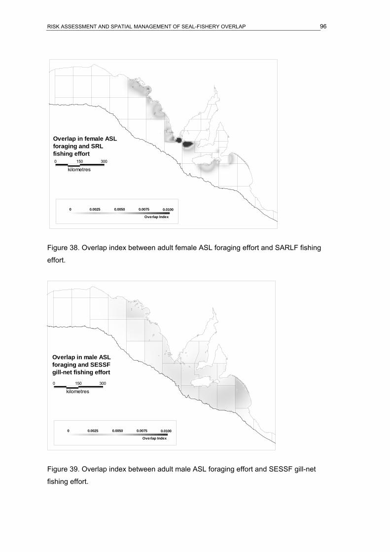
RISK ASSESSMENT AND SPATIAL MANAGEMENT OF SEAL-FISHERY OVERLAP 96
150
kilometres0 300
Overlap in female ASL foraging and SRL fishing effort
0.0100
Overlap Index
0.00750.00500 0.0025
Figure 38. Overlap index between adult female ASL foraging effort and SARLF fishing
effort.
150
kilometres0 300
Overlap in male ASL foraging and SESSF gill-net fishing effort
0.0100
Overlap Index
0.00750.00500 0.0025
Figure 39. Overlap index between adult male ASL foraging effort and SESSF gill-net
fishing effort.

RISK ASSESSMENT AND SPATIAL MANAGEMENT OF SEAL-FISHERY OVERLAP 97
150
kilometres0 300
Overlap in male ASL foraging and SRL fishing effort
0.0100
Overlap Index
0.00750.00500 0.0025
Figure 40. Overlap index between adult male ASL foraging effort and SARLF fishing
effort.
150
kilometres0 300
Overlap in subadult male ASL foraging and SESSF gill-net fishing effort
0.0100
Overlap Index
0.00750.00500 0.0025
Figure 41. Overlap index between sub-adult male ASL foraging effort and SESSF gill-net
fishing effort.

RISK ASSESSMENT AND SPATIAL MANAGEMENT OF SEAL-FISHERY OVERLAP 98
150
kilometres0 300
Overlap in subadult male ASL foraging and SRL fishing effort
0.0100
Overlap Index
0.00750.00500 0.0025
Figure 42. Overlap index between sub-adult male ASL foraging effort and SARLF fishing
effort.
150
kilometres0 300
Overlap in juvenile ASL foraging and SESSF gill-net fishing effort
0.0100
Overlap Index
0.00750.00500 0.0025
Figure 43. Overlap index between juvenile ASL foraging effort and SESSF gill-net fishing
effort.

RISK ASSESSMENT AND SPATIAL MANAGEMENT OF SEAL-FISHERY OVERLAP 99
150
kilometres0 300
Overlap in juvenile ASL foraging and SRL fishing effort
0.0100
Overlap Index
0.00750.00500 0.0025
Figure 44. Overlap index between juvenile ASL foraging effort and SARLF fishing effort.
150
kilometres0 300
Overlap in ASL pup foraging and SESSF gill-net fishing effort
0.0100
Overlap Index
0.00750.00500 0.0025
Figure 45. Overlap index between ASL pup foraging effort and SESSF gill-net fishing
effort.

RISK ASSESSMENT AND SPATIAL MANAGEMENT OF SEAL-FISHERY OVERLAP 100
150
kilometres0 300
Overlap in ASL pup foraging and SRL fishing effort
0.0100
Overlap Index
0.00750.00500 0.0025
Figure 46. Overlap index between ASL pup foraging effort and SARLF fishing effort.
Figure 47. Estimated proportion of ASL subpopulations that achieve quasi-extinction as a
function of the number of additional pre-recruit female mortalities/subpopulation/year.
Three scenarios are given, based on the increasing (r=0.05), stable (r=0.00) and
declining (r=-0.01) population models.

RISK ASSESSMENT AND SPATIAL MANAGEMENT OF SEAL-FISHERY OVERLAP 101
-3.5
-3.0
-2.5
-2.0
-1.5
-1.0
-0.5
0.0
0 5 10 15 20 25 30
Rat
e of
pop
ulat
ion
decl
ine
(%/y
ear)
Age (years)
Figure 48. Simulated example of how the stage (age) at which mortalities are taken
affects the rate of population change. In this example a subpopulation of 1,000 female
ASL has 20 females removed from a particular age-group each year for 50 reproductive
cycles (75 years), using the stable population model (r=0). The rate of population decline
resulting from each scenario is presented, fitted with a 4th order polynomial curve. The
example demonstrates how the rate of decline is affected by the age-group of females
removed from the population. The greatest rates of decline are achieved when 4.5-6, 6-
7.5 and 7.5-9 age-group females are removed.

RISK ASSESSMENT AND SPATIAL MANAGEMENT OF SEAL-FISHERY OVERLAP 102
GA
B B
2
Sout
h N
eptu
ne Is
.
Glid
don
Ree
f
War
d Is
.
Mas
illon
Is.
Seal
Slid
e
GA
B B
6
Four
Hum
moc
ks Is
.
Nor
th N
eptu
ne (E
ast)
Is.
Wes
tern
Nuy
ts R
eef
Jone
s Is
.
Alb
atro
ss Is
.
GA
B B
1
Roc
ky (N
orth
) Is.
GA
B B
9
Bre
akw
ater
Ree
f
Fene
lon
Is.
Pea
ked
Roc
k
Pric
e Is
.
Loun
ds Is
.
Pea
rson
Is.
Nor
th Is
.
Engl
ish
Is.
GA
B B
3
GA
B B
8
Ligu
anea
Is.
GA
B B
5
Wes
t Is.
East
Fra
nklin
Ree
f
Nic
olas
Bau
din
Is.
Lew
is Is
.
Wes
t Fra
nklin
Ree
f
Oliv
e Is
.
Pur
die
Is.
Wes
t Wal
degr
ave
Is.
Sea
l Bay
The
Page
s
Dan
gero
us R
eef
100
80
60
40
Very High High Risk Moderate Risk Low
Risk Risk
Figure 49. Bray-Curtis similarity matrix dendrogram of SA ASL subpopulations, which are
clustered according to percentage similarity of quasi-extinction risk (from PVA outputs).
Four main groups are identified as the different Risk Categories (dendrogram produced
using Primer V5.2.2).

RISK ASSESSMENT AND SPATIAL MANAGEMENT OF SEAL-FISHERY OVERLAP 103
Figure 50. Estimated proportion of historic bycatch (broken down by seal sex) accounted
for by each SA ASL subpopulation in the SESSF gillnet sector (top plot) and the SARLF
(bottom plot).

RISK ASSESSMENT AND SPATIAL MANAGEMENT OF SEAL-FISHERY OVERLAP 104
A.
0.00
0.05
0.10
0.15
0.20
0.25
The
Page
s
Kang
aroo
Isla
nd
Sou
th S
penc
er G
ulf
SW
Eyr
e
Wes
t Eyr
e
Cha
in o
f Bay
s
Gre
ater
Nuy
ts
GA
B
FemalesMales
Estim
ated
pro
port
ion
of A
SL b
ycta
ch p
er re
gion
(gill
net s
ecto
r SES
SF)
B.
0.00
0.05
0.10
0.15
0.20
0.25
The
Page
s
Kan
garo
o Is
land
Sout
h Sp
ence
r Gul
f
SW E
yre
Wes
t Eyr
e
Cha
in o
f Bay
s
Gre
ater
Nuy
ts
GA
B
Females
Males
Estim
ated
pro
port
ion
of A
SL b
ycta
ch p
er re
gion
(SR
L fis
hery
)
Figure 51. Estimated proportion of historic bycatch (broken down by seal sex) accounted
for by regional groupings of SA ASL subpopulations in the SESSF gillnet sector (top plot)
and the SARLF (bottom plot).

RISK ASSESSMENT AND SPATIAL MANAGEMENT OF SEAL-FISHERY OVERLAP 105
Figure 52. Estimated proportion of historic bycatch (broken down by seal sex) (1973-
2004) in SA for ASL accounted for by each SESSF gillnet sector MFA.
Figure 53. Estimated proportion of historic (1970-2004) bycatch (broken down by sex) in
SA for ASL accounted for by each SA RLF MFA.

RISK ASSESSMENT AND SPATIAL MANAGEMENT OF SEAL-FISHERY OVERLAP 106
0
0.1
0.2
0.3
0.4
0.5
0.6
1970 1975 1980 1985 1990 1995 2000 2005
Prop
ortio
n A
SL b
ycat
ch p
er re
gion
(gill
net S
ESSF
) The PagesKangaroo IslandSouthern Spencer GulfSW EyreWest EyreChain of BaysGreater NuytsGAB
Figure 54. Estimated temporal change in the proportion of historic (1973-2004) SA
SESSF gillnet sector bycatch, of ASL from different geographic regions.
0
5
10
15
20
25
30
35
40
1970 1975 1980 1985 1990 1995 2000 2005
Hyp
othe
tical
ASL
byc
atch
per
yea
r (gi
llnet
SES
SF)
The PagesKangaroo IslandSouthern Spencer GulfSW EyreWest EyreChain of BaysGreater NuytsGAB
Figure 55. Hypothetical temporal change in the numbers of historic (1973-2004) SA
SESSF gillnet sector bycatch, of ASL from different geographic regions. Numbers based
on a hypothetical bycatch rate of 0.005 seals/km of net-lift.

RISK ASSESSMENT AND SPATIAL MANAGEMENT OF SEAL-FISHERY OVERLAP 107
0.0
0.1
0.2
0.3
0.4
0.5
1970 1975 1980 1985 1990 1995 2000 2005
Prop
ortio
n A
SL b
ycat
ch p
er re
gion
(SR
L fis
hery
) The PagesKangaroo IslandSouthern Spencer GulfSW EyreWest EyreChain of BaysGreater NuytsGAB
Figure 56. Estimated temporal change in the proportion of historic (1970-2004) SA RLF
bycatch, of ASL from different geographic regions.
0
5
10
15
20
25
30
35
40
1970 1975 1980 1985 1990 1995 2000 2005
Hyp
othe
tical
ASL
byc
atch
per
yea
r (SR
L Fi
sher
y)
The PagesKangaroo IslandSouthern Spencer GulfSW EyreWest EyreChain of BaysGreater NuytsGAB
Figure 57. Hypothetical temporal change in the numbers of historic (1970-2004) SA RLF
sector bycatch, of ASL from different geographic regions. Numbers based on a
hypothetical bycatch rate of 0.2 seals/1,000 pot-lifts.

RISK ASSESSMENT AND SPATIAL MANAGEMENT OF SEAL-FISHERY OVERLAP 108
0
0.1
0.2
0.3
0.4
0.5
0.6
1970 1975 1980 1985 1990 1995 2000 2005
Prop
ortio
n A
SL b
ycat
h pe
r MFA
(gill
net S
ESSF
)
108115129144149150
Figure 58. Estimated temporal change in the proportion of historic (1973-2004) SA
SESSF gillnet sector bycatch, from the six major contributing MFAs for ASL.
0
10
20
30
40
50
60
70
1970 1975 1980 1985 1990 1995 2000 2005
Hyp
othe
tical
ASL
byc
ath
per M
FA (g
illne
t SES
SF)
108115129144149150
Figure 59. Hypothetical temporal change in the numbers of historic (1973-2004) SA
SESSF gillnet sector bycatch, from the six major contributing MFAs for ASL . Numbers
based on a hypothetical bycatch rate of 0.005 seals/km of net-lift.
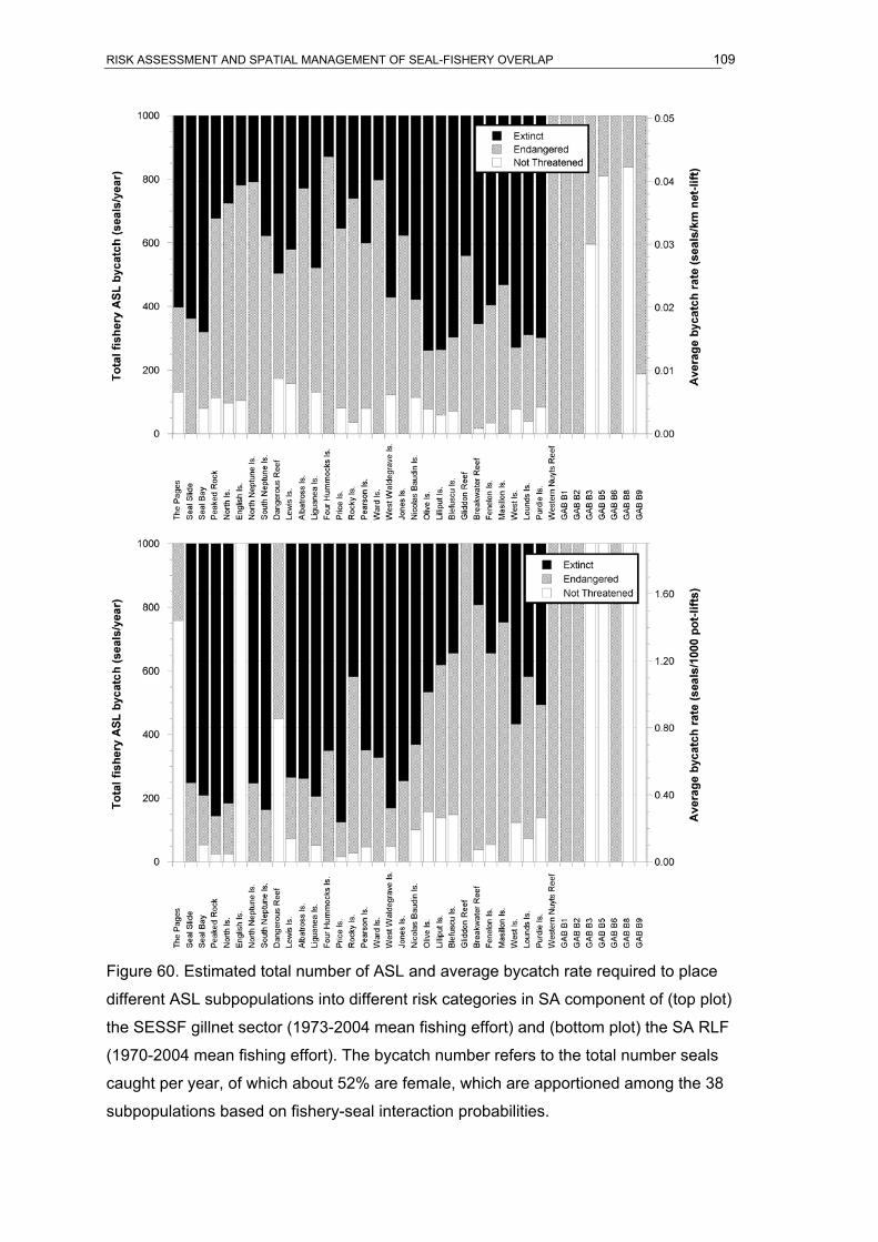
RISK ASSESSMENT AND SPATIAL MANAGEMENT OF SEAL-FISHERY OVERLAP 109
Figure 60. Estimated total number of ASL and average bycatch rate required to place
different ASL subpopulations into different risk categories in SA component of (top plot)
the SESSF gillnet sector (1973-2004 mean fishing effort) and (bottom plot) the SA RLF
(1970-2004 mean fishing effort). The bycatch number refers to the total number seals
caught per year, of which about 52% are female, which are apportioned among the 38
subpopulations based on fishery-seal interaction probabilities.

RISK ASSESSMENT AND SPATIAL MANAGEMENT OF SEAL-FISHERY OVERLAP 110
0
0.1
0.2
0.3
0.4
0.5
0.6
1970 1975 1980 1985 1990 1995 2000 2005
Prop
ortio
n A
SL b
ycat
h pe
r MFA
(SR
L Fi
sher
y
8
15
28
39
49
Figure 61. Estimated temporal change in the proportion of historic (1970-2004) SARLF
bycatch, from the major contributing MFAs for ASL.
0
10
20
30
40
50
1970 1975 1980 1985 1990 1995 2000 2005
Hyp
othe
tical
ASL
byc
ath
per M
FA (S
RL
Fish
ery) 8
15283949
Figure 62. Hypothetical temporal change in the numbers of historic (1970-2004) SA RLF
bycatch, from major contributing MFAs for ASL. Numbers based on a hypothetical
bycatch rate of 0.2 seals/1,000 pot-lifts.

MOLECULAR DNA TECHNIQUES TO DETERMINE THE DIET OF SEA LIONS 111
DEVELOPING MOLECULAR DNA TECHNIQUES TO DETERMINE THE DIET OF AUSTRALIAN SEA LIONS
Kristian Peters1,2,3, Kathy Ophelkeller1 and Simon D. Goldsworthy3 1 South Australian Research and Development Institute (Sustainable Systems – Plant
and Soil Health), GPO Box 397, Adelaide South Australia 5001 2 School of Earth and Environmental Sciences, University of Adelaide, Adelaide, South
Australia 5005 3 South Australian Research and Development Institute (Aquatic Sciences), PO Box 120,
Henley Beach, South Australia 5022
Introduction
Analysing dietary remains of marine mammals can enhance our understanding of the
temporal and spatial trophodynamics of marine ecosystems. Dietary remains from
digestive tracts have been used to diagnose prey in a number of pinniped species
(Gales and Cheal 1992; Alonso et al. 2000; Yonezaki et al. 2003; McIntosh et al. 2006),
as have regurgitates (Fea et al. 1999; Childerhouse et al. 2001; Page et al. 2005) and
scats (Goldsworthy et al. 1997; Bowen 2000; Anderson et al. 2004). The collection and
visual identification of indigestible hard-prey structures, such as bones, scales,
exoskeleton, and eye lenses can often provide a useful means to diagnose prey to
genus or species level (Boyle and Pierce, 1991), and is a successful method of retrieving
large quantities of dietary information, mostly using a relatively simple, non-invasive
approach (Gales and Pemberton 1994; Gales et al. 1993; Childerhouse et al. 2001).
Where sagittal otoliths and cephalopod beaks are recovered and can be identified
(Casaux et al. 2003; de Bruyn et al. 2003; Hume et al. 2004; Page et al. 2005, McIntosh
et al. 2006), the number and size of prey ingested can be approximated (Bowen 2000).
This is of importance when providing representative qualitative and quantitative
measures of the relative biomass of each prey species consumed (Hyslop, 1980).
Studies that require prey remnants to be recovered from faecal, stomach, and
regurgitate samples have some biases, which stem from the differential digestion,
passage and retention rates of prey consumed (Dellinger and Trillmich 1987; Gales and
Pemberton, 1990; Gales and Cheal, 1992; Cottrell et al. 1996). These biases are
heightened in ASL, because of prolonged retention rates which may facilitate the

MOLECULAR DNA TECHNIQUES TO DETERMINE THE DIET OF SEA LIONS 112
complete digestion of prey in the gastrointestinal tract (Gales and Cheal, 1992). Feeding
trials and recent stomach analyses of ASL (Richardson and Gales,1987; Gales and
Cheal, 1992; McIntosh et al. 2006) also demonstrate that complete digestion of fish
otoliths and retention or regurgitation of other prey structures limits the use of
morphological prey identification of diet remains.
Even though these biases confound the use of traditional diet analysis, information on
the trophic interactions of ASL across their geographical range remains restricted and is
based on few published diet accounts recording a range of benthic prey species
including crustaceans; rock lobster (Panulirus cygnus and Jasus sp.), swimming crab
(Ovalipes australiensis), various cephalopods; cuttlefish (Sepia sp.), squid (Sepioteuthis
australis and Nototodarus gouldi), octopus, fish; whiting (Sillaginodes punctata) leather
jacket (Monocanthidae), flathead (Neoplatycephalus sp.), swallowtail (Centroberyx
lineatus), common bullseye (Pempheris multiradiata), eastern school whiting (Sillago
flindersi), yellowtail scad (Trachurus novaezelandiae), Australian salmon (Arripis
truttaceus), sharks; school shark (Galeorhinus galeus) and gummy shark (Mustelus
antarcticus) and birds; little penguin (Eudyptula minor) (Walker and Ling (1981);
Richardson and Gales (1987); Gales and Cheal (1992); Ling (1992); McIntosh et al.
2006).
The recent use of molecular genetics to determine relationships between predators and
the prey they consume is gaining popularity in diet studies where stomach or faecal
contents are morphologically unrecognisable. Polymerase chain reaction (PCR) based
techniques using species-specific and group-specific primers have successfully detected
krill as a prey species from pygmy blue whale (Balaenoptera musculus brevicauda), fin
whale (Balaenoptera physalus) (Jarman et al. 2002), and whale shark (Rhincodon typus)
faeces (Jarman et al. 2002). Fish and krill have been identified from DNA refined from
the stomach contents of giant squid (Architeuthis sp.) (Deagle et al. 2005b) and scats
from Adélie penguins (Pygocelis adeliae) (Jarman et al. 2002). Teleost fish and
cephalopod prey DNA have been distinguished in Steller sea lion (Eumetopias jubatus),
Antarctic and New Zealand fur seal scats collected from captive (Deagle et al. 2005a;
Deagle et al. 2006; Deagle and Tollit 2007; Casper et al. 2007b) and wild seals (Casper
et al. 2007a). This technique has shown potential to be an effective method for diet
assessment for ASL.
A recent report to the Department of Environment and Heritage, which formed the basis
for a Draft Recovery Plan for the species, detailed the impediments to growth in ASL

MOLECULAR DNA TECHNIQUES TO DETERMINE THE DIET OF SEA LIONS 113
populations (McKenzie et al. 2005). The report identified the development of techniques
to provide quantitative analyses of sea lion diets as a key research priority, with faecal
DNA assessment appearing the most promising technique.
Captive feeding experiments are necessary to assess the suitability of using faecal DNA
analysis to provide a quantitative estimate of prey composition in the diet of ASL. The
development of these methods, which forms the basis of this research, could provide key
information to assist in the recovery of the species, especially the identity of key prey
species, which may have limited distributions or habitats. Additionally, we will gain a
better understanding of the extent of trophic interactions and the level of which ASL
target commercially important species.
Methods
Trial animals and feeding trial enclosures
Two long-term captive ASL (Neophoca cinerea) (one 6 year old male and one 26 year
old adult female) were used in a captive feeding trial conducted at the Adelaide
Zoological Gardens, South Australia, between January and February 2006. Sea lions
were chosen on individual health but also on their ability to show consistency when
consuming food on a regular basis.
The female and the male were housed separately during daylight hours (~ 8 -10 hrs/day)
but overnight the female was housed with a third sea lion (~ 14 hrs / day). The male was
displayed during daylight hours with a third sea lion but isolated in the evenings.
Because the trials were conducted over the Australian summer, the main display
enclosure contained a large salt chlorinated pool (11m x 8m x 2m) while evening
enclosures contained a shallow pool with sprinkler system.
Trial duration and diet protocols
The adult male was fed experimental diets, which contained cephalopods and shark
(novel diet) and fish (normal diet). The adult female was fed a control diet, which was
entirely fish. Sea lion mass was recorded throughout the duration of the trial. Because
some remains of food may be retained by captive ASL for >96 h (4 days) (Richardson
and Gales, 1987; Gales and Cheal, 1993; Bodley et al. 1999), the feeding trial was

MOLECULAR DNA TECHNIQUES TO DETERMINE THE DIET OF SEA LIONS 114
divided into 4 weekly periods. The study commenced with a 5 day period, during which
novel prey were not fed to the male. Different experimental diets were then fed each
week for 4 weeks. The trial ended after a 14-day period, when no novel prey were fed to
the male, to assess retention times of novel prey (Figure 63).
0
10
20
30
40
50
60
70
80
90
100
Pre trial control Exp. diet w k1 Exp. diet w k2 Exp.diet w k3 Exp. diet w k4 Post trialcontrol w k 6+7
Prop
ortio
n of
mea
l fed
(%)
(M2) 5.7kg novel+fish prey
(M2) 5.7kg fish only
(M1) 300gm fish only
0 47
5d 7d 7d 7d 7d 14d
(A)
Days
0
10
20
30
40
50
60
70
80
90
100
Pre trial control Control w k1 Control w k2 Control w k3 Control w k4 Post trial controlw k 6+7
Prop
ortio
n of
mea
l fed
(%)
(M2) 5.7kg f ish only
(M1) 300gm fish only
5d 7d7d7d 7d 14d
Days0 47
(B)
Figure 63. Feeding trial duration (days) and meals fed (%) during mornings (M1) and
evenings (M2) to the male (A) and female (B) ASL at the Adelaide Zoo between January
and February 2006. Arrows indicate the control periods (only fish and no novel prey).
Novel prey and fish introduced into the diet (hashed columns) for 4 weeks. Values above
columns are number of days that each diet was fed.
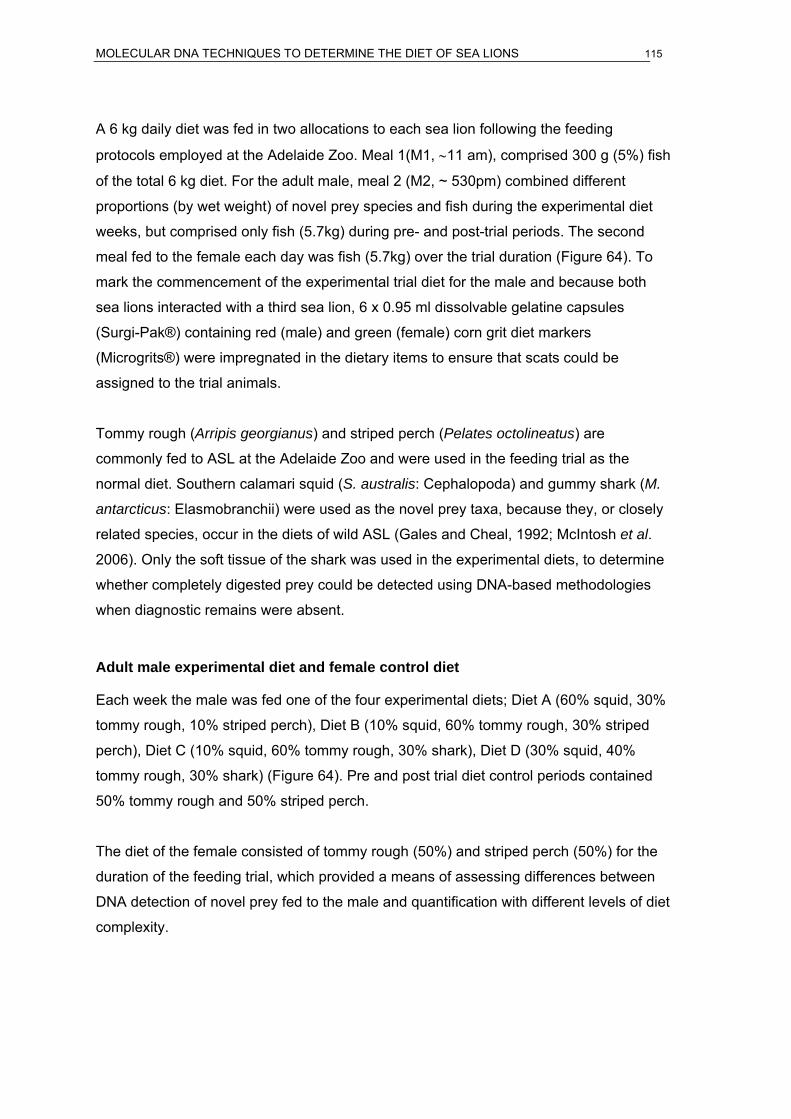
MOLECULAR DNA TECHNIQUES TO DETERMINE THE DIET OF SEA LIONS 115
A 6 kg daily diet was fed in two allocations to each sea lion following the feeding
protocols employed at the Adelaide Zoo. Meal 1(M1, ∼11 am), comprised 300 g (5%) fish
of the total 6 kg diet. For the adult male, meal 2 (M2, ~ 530pm) combined different
proportions (by wet weight) of novel prey species and fish during the experimental diet
weeks, but comprised only fish (5.7kg) during pre- and post-trial periods. The second
meal fed to the female each day was fish (5.7kg) over the trial duration (Figure 64). To
mark the commencement of the experimental trial diet for the male and because both
sea lions interacted with a third sea lion, 6 x 0.95 ml dissolvable gelatine capsules
(Surgi-Pak®) containing red (male) and green (female) corn grit diet markers
(Microgrits®) were impregnated in the dietary items to ensure that scats could be
assigned to the trial animals.
Tommy rough (Arripis georgianus) and striped perch (Pelates octolineatus) are
commonly fed to ASL at the Adelaide Zoo and were used in the feeding trial as the
normal diet. Southern calamari squid (S. australis: Cephalopoda) and gummy shark (M.
antarcticus: Elasmobranchii) were used as the novel prey taxa, because they, or closely
related species, occur in the diets of wild ASL (Gales and Cheal, 1992; McIntosh et al.
2006). Only the soft tissue of the shark was used in the experimental diets, to determine
whether completely digested prey could be detected using DNA-based methodologies
when diagnostic remains were absent.
Adult male experimental diet and female control diet
Each week the male was fed one of the four experimental diets; Diet A (60% squid, 30%
tommy rough, 10% striped perch), Diet B (10% squid, 60% tommy rough, 30% striped
perch), Diet C (10% squid, 60% tommy rough, 30% shark), Diet D (30% squid, 40%
tommy rough, 30% shark) (Figure 64). Pre and post trial diet control periods contained
50% tommy rough and 50% striped perch.
The diet of the female consisted of tommy rough (50%) and striped perch (50%) for the
duration of the feeding trial, which provided a means of assessing differences between
DNA detection of novel prey fed to the male and quantification with different levels of diet
complexity.

MOLECULAR DNA TECHNIQUES TO DETERMINE THE DIET OF SEA LIONS 116
0
10
20
30
40
50
60
70
80
90
100
Pre trial control Diet A Diet B Diet C Diet D Post trialcontrol
Prop
ortio
n of
die
t (%
)Gummy shark
S.perch
T.rough
Calamari squid
A
B C
D
5d 7d 7d 7d 7d 14d
(A)
1 2
0
10
20
30
40
50
60
70
80
90
100
Pre trial control Trial control Trial control Trial control Trial control Post trial control
Prop
ortio
n of
die
t (%
)
S.perch
T.rough
7d 7d 7d 7d 7d 14d
(B)
Figure 64. Prey species contributions (%) in the 6kg diet fed to the ASL male (A) and
female (B). A, B, C, and D are experimental diets consisting of novel prey; squid and
shark, combined with 2 fish species, including tommy rough and striped perch. The
female diet (B) was tommy rough (3kg) and striped perch (3kg) in equal proportions.
Columns (1, 2) are normal diets (2 fish species and no novel prey) to compare DNA
detection signals of novel prey fed during experimental diets A, B, C, and D. Values
above columns are number of days fed for each diet.

MOLECULAR DNA TECHNIQUES TO DETERMINE THE DIET OF SEA LIONS 117
Collection and storage of faecal samples
Faecal samples were collected for the duration of the trial (48 days). Each morning the
enclosures were checked for faecal samples and then hosed clean. Enclosures were
checked for samples at every hour from 7am until 12pm and every 2 h until 530 pm. All
pools were fitted with 100μm fine drain outlet filters to retain scats in pools, before the
pools were cleaned each day. Scats were stored in sterile 500ml Nasco Twirl® double
sealed bags, which contained a 1:4 ratio of scat to 99.7% ethanol (Murphy et. al. 2002,
Vink et al. 2005). The ethanol and the scat was homogenised to preserve the DNA and
stored at –20C.
For long term DNA preservation, each faecal sample was freeze-dried using a Cuddon™
Freeze-Dryer (model GP 1015FD) with shelf temperature of 40 C and final pressure of 2
Torr. This approach can significantly increase DNA amplification success rates during
PCR assays (Murphy et al. 2000). The ethanol/scat slurry was homogenised, a sub
sample was removed then placed into a collection cylinder to settle. With supernatant
removed, samples were freeze-dried. Once dry, each sample was finely ground and the
resultant scat dust homogenised dry through inversion.
Prey morphological analysis
Prey remains were isolated from ethanol/scat slurry by washing through a series of 3
nested sieves of decreasing size (smallest 100μm). Sagittal otoliths and squid beaks
were stored dry and other remains were stored in plastic vials with 90% ethanol. The
faecal sample collected from the male and the 3 from the female in the pre-trial period
were excluded from the hard-prey analysis to ensure that prey consumed prior to the
feeding trial was excluded from all analyses.
All otoliths were photographed and measured (Image pro 5.1) using a Leica digital
microscope, which was calibrated at magnification of x 0.71. Where possible, otoliths
were identified as being from the left or right side, identified to species and categorised
according to the level of erosion (adapted from Hull et al. 1999). Categories were: 1)
unrecognisable to species; heavily worn, no distinguishable features, no rostrum, no
ventral crenulations, very slight or no sulcus, featureless disk, 2) identifiable to species;
with slightly visible sulcus, mostly unrecognisable features, no rostrum, few visible
ventral crenulations, exterior worn; 3) identifiable to species; visible and definite sulcus,

MOLECULAR DNA TECHNIQUES TO DETERMINE THE DIET OF SEA LIONS 118
slight rostrum or not present, slight ventral crenulations but worn, 4) identifiable to
species; intact sulcus, partial rostrum, ventral crenulations marginal and slightly worn,
and 5) identifiable to species; pristine otolith with undamaged sulcus and rostrum, ventral
crenulations pronounced. Frequency of occurrence and numerical abundance estimates
were determined. Reconstructed fish mass (wet weight/kg) was calculated based on the
minimum number of individuals identified in each scat, using weight data collected from
fresh fish.
Faecal DNA extraction
Two DNA extraction methods were compared to isolate DNA from scats. Five faecal
samples were randomly chosen and DNA from 500mg of the re-homogenised freeze-
dried sample was extracted using 1) QiAmp® DNA Mini Stool Kit (Qiagen, 2007) and 2)
an in-house extraction facility (SARDI, 2007). DNA extracted from faecal samples
contained 2 extraction blanks (reagents only) as an internal control to screen for cross
contamination. DNA yield was quantified by fluorescence of 2μl x 5 replicates of each
sample using Picogreen dsDNA Quantitation reagent (Molecular Probes-Invitrogen®) on
a Wallac1420 multilabel fluorometer with fluorescence set to read at 485nm/535nm for
0.1sec. Because DNA from scats is typically of poor quality (Murphy et al. 2000; Deagle
et al. 2005; Deagle et al. 2006) SARDI in-house facility was used because commercial
extraction kits consistently yielded 1000pg less DNA. Replicate PCR assays containing
DNA from both extraction methods were tested using PCR and gel electrophoresis. DNA
from 58 faecal samples (male = 28; female = 30) was extracted. Each sample was
randomly given a reference number (1-58) to eliminate bias when scoring PCR products.
Prey tissue DNA extractions
DNA taken from the tissue of sharks and squid was removed from internal tissues, which
could not have been exposed to foreign DNA. Samples were washed in dilute 1:20
Tween® and RNA free water and 15mg was removed for DNA purification using Qiagen
DNeasy Tissue kits. A final elution of 100μl was used to increase the final DNA
concentration of each sample. Sample contamination was monitored using extraction
blanks while aerosol resistant filter pipette tips were used to avoid cross contamination
between samples.

MOLECULAR DNA TECHNIQUES TO DETERMINE THE DIET OF SEA LIONS 119
Primer development
Short, species-specific primer sets of <100 base pairs were constructed to amplify and
quantify DNA for each dietary species in the feeding trials (Table 17). Mitochondrial DNA
was chosen because it is often in higher concentration than nuclear DNA within faeces
(Birky et al. 1989) and preserves well during the freeze-drying process (Murphy et. al.
2002). Sequences were aligned using the Bioedit®: Biological sequence alignment editor
(Ibis Biosciences, 2007) and primer pairs constructed using ABI Primer Express V 2.0®
(Applied Biosystems) with amplicon parameters set to distinguish between 50 and
100bp. The BLAST algorithm (Altschul et al.1997) was used to screen primer sets for
specificity and assess the level of similarity against sequences in Genbank. Primer
sequences were tested against aligned sequences in Bioedit and assessed for sequence
specificity.
Primer optimisation and Qualitative Standard PCR amplification
Because faecal DNA is a combination of digested prey and the defecator’s gut bacteria
and exfoliated gastrointestinal epithelial cells (Albaugh et al. 1992), primer sets screened
DNA for the target species and all non-target trial prey and sea lion DNA. Initial PCR
assays were optimised using temperature and MgCl2 concentration gradients which
varied between 55 oC and 65 oC and 1.0mM and 2.5mM MgCl2 (final concentration)
generated on either PTC-200 or PTC-225 Peltier Gradient Block Thermal Cyclers (MJ
Research).
Optimised primer sets for amplifying shark DNA, consisted of 25μl PCR reactions
containing 2μl DNA template, 0.5μl 2.0mM MgCl2, 2.5μl 10 x Qiagen PCR buffer, 0.2μl 1
x BSA (Bovine serum albumin), 0.5μl 0.2μM DNTP, 0.5μl 0.4μM forward and reverse
primer, and 1 x Hotstar Taq polymerase (Qiagen). Thermal cycling conditions were 95 oC
for 15 min, then 94 oC for 2 min, followed by 32 cycles of 94 oC for 10 s, 64.1 oC for 30 s,
72 oC for 30 s with final extension of 72 oC for 10 min. A 20μl volume for squid PCR
reactions contained the same concentration and volumes of all reagents as shark PCR,
except 2.5μl 15mM MgCl2 (contained within PCR Buffer) was used. Thermal cycling
conditions were 95 oC for 15 min, then 94 oC for 2 min, followed by 32 cycles of 94 oC for
10 s, 60.0oC for 30 s, 72 oC for 30 s with final extension of 72 oC for 10 min.
Detection of PCR products was determined by electrophoresis on ethidium-bromide
stained 1.5% agarose gel. Product bands were visualised using Gel-DOC UV illuminator
(Bio-Rad®) supported by Quantity One-Quantitation analysis software (Bio-Rad®).

MOLECULAR DNA TECHNIQUES TO DETERMINE THE DIET OF SEA LIONS 120
Replicates of successful PCR amplifications were performed to confirm that positive
results were not due to false-positives from the first PCR attempt. All PCRs were blind
scored to remove scoring bias.
Quantitative PCR amplification - Real time PCR
Quantitative estimates for the relative amount of DNA of each prey species were
achieved using real-time quantitative qPCR reagent PowerSybr Green (Applied
BioSystems) on an ABI prism® Real–time 7900HT sequence detection system (Applied
BioSystems).
DNA reference standards (8 lambda) with known concentrations of DNA (between 0
ng/μl to 12ng/μl) were developed in triplicate and fitted to a standard curve (Figure 65).
The concentration of DNA from squid and shark tissue was estimated against λ standard
values and the exact DNA concentration (pg/μl) was determined (shark 5845 pg/μl, squid
33017 pg/μl) (Figure 65). The cycle threshold (Ct) values for each prey species standard
curve plots were set at 0.1 determined PCR assay sensitivity for detecting DNA of shark
and squid at 2fg/μl and 20fg/μl respectively.
y = 1039.6x + 69.792R2 = 0.9993
0
2000
4000
6000
8000
10000
12000
14000
0 2 4 6 8 10 12
Lambda DNA (ng/ul)
pGre
en (C
ount
s)
Figure 65. Standard curve from 8 Lambda (λ) DNA diluted standards (0 ng/μl to12 ng/μl)
and PicoGreen counts. Series dilutions (0-200000 fg/μl) of DNA (extracted from shark
and squid tissue) are quantified against the known (λ) DNA. Relative amounts of gummy
shark and squid dsDNA within faecal samples are determined against these values.
Quantitative estimates of prey DNA from scats were determined using primers and real-
time PCR. Power SYBR Green® contains the fluorescent marker SYBR green that binds
to all double-stranded DNA (dsDNA) during PCR. Real-time PCR reactions contained 4μl
faecal DNA template, and 6μl Power SYBR Green master mix (final concentration 0.4μM
and 1X ABI PCR mastermix). Cycling conditions for each PCR reaction followed default
Power SYBR Green protocols with activation time of polymerase at 95 oC 10 min,

MOLECULAR DNA TECHNIQUES TO DETERMINE THE DIET OF SEA LIONS 121
followed by 40 cycles of 95 oC 15 s, and 60 oC 1 min, and a dissociation stage (95 oC 15
s, 60 oC 15 s, 95 oC 15 s) for both squid and shark primers.
Cloning and sequencing
PCR products that produced visible bands using gel electrophoresis were excised and
purified using a Nucleospin® Extract II PCR cleanup gel extraction kit (Macherey-Nagel).
Samples were cloned into a pGEM®-T easy cloning vector (Promega) for DNA
sequencing. For each sample, 2 transformation cultures containing transformed
Escherichia coli cells were plated and grown to generate transformant colonies. Eight
white colonies per sample provided the DNA template for the SP6/T7 (vector primers) for
standard (25μl) PCRs, which were designed for positive identification of the insert.
Thermal-cycling conditions were 95 oC 15 min, 94 oC 1 min, followed by 29 cycles of 48 oC 45 s, 72 oC 45 s, then 72 oC 8 min, 4 oC 5 min. Cultivated bacterial cells (3 ml) were
centrifuged and the remaining supernatant was removed. Plasmid DNA from the
bacterial cells was purified using a NucleoSpin® Plasmid DNA purification kit (Machery-
Nagel). Genetic sequences were generated at the Australian Genomic Research Facility
using 5.5μl plasmid DNA combined with 2.6μl (20μM) Sp6/T7 primer.
Results
Mean body mass of male and female captive ASL fluctuated during the 47 day trial
between (± 3.5 kg) and (± 5.75 kg) from the pre-trial mass of 200kg and 100kg
respectively.
Prey remains from sample collections
In total, 58 faecal samples were collected and assigned to an individual seal (male = 28,
female = 30).Two scats were collected intact from the main display pool and identified
from diet markers as having been produced by the male. Scats were not collected from
night enclosure pools. Twelve (43%) scats were collected from the male over control
diets, while 3 (11%), 3 (11%), 2 (7%), and 8 (28%) scats were collected during Diet A, B,
C and D respectively. Squid was increased to 30% in the final 2 days of Diet C because
only one scat was collected 6 days after the initial consumption of shark. Multiple scats
(2 and 3) were collected on 3 mornings during Diet D. One regurgitate containing
unidentifiable tissue was collected. Highly eroded vertebral processes, eye lenses and
MOLECULAR DNA TECHNIQUES TO DETERMINE THE DIET OF SEA LIONS 122
scales of fish were present in 23 (82%) of male scats, but could not be identified to
species and were not used in the analysis.
Only one fish otolith (<1%) was recovered from 6674 otoliths consumed by the female.
Other hard remains were limited to 2 unidentifiable vertebrae, scales and fragments of
eye lenses. Although 61% (17/28) of scats from the male contained otoliths, only 2% of
all otoliths consumed (110 out of 5170) were recovered. Thirteen otoliths were identified
as striped perch, 70 were tommy rough and 27 (25%) were heavily eroded and could not
be assigned to species (Table 16). There was no relationship between the number, and
type of fish species fed, to the number of otoliths recovered (r2 =.001, n = 7, P = 0.941),
while otolith recovery rates were not related to the size of otoliths ingested (χ2 = 0.077, df
= 1, P = 0.782). Reconstructed mass recovery estimates (% wet weight/kg) for the fish
component of the diet were low for both species (~1% recovered of mass ingested),
except diet A (4%) (Table 18). Squid beaks were not recovered from scats from the 116
ingested.
Table 16. Frequency of occurrence (FOO) and numerical abundance (NA) of diagnostic
hard remains (otoliths) identified from scats (n = 28) collected from the male ASL during
feeding trials. Diagnostic remains from squid were not recovered.
FOO NACommon name Species n % n %
Tommy rough Arripis georgianus 13 46.4 70 63.6
Striped perch Pelates octolineatus 5 17.9 13 11.8
Unknown otoliths Not identified 10 35.7 27 24.6
Calamari squid Sepioteuthis australis 0 0 0 0Gummy shark Mustelus antarcticus - - - -
Primer assessment
Primer amplicon size affected amplification success rates for detecting gummy shark and
squid DNA from scats. Six primer sets (>100bp) were optimised for detecting gummy
shark and squid DNA but no products were amplified. Small primer sets (<100bp)
designed to detect shark and squid DNA were successful (Table 17).

MOLECULAR DNA TECHNIQUES TO DETERMINE THE DIET OF SEA LIONS 123
Table 17. PCR primers tested in standard and real-time quantitative PCR for detecting
squid and shark in sea lion scats. Successful primer sets (+) in bold. All other primers
amplified target taxon DNA but not prey DNA from sea lion faeces (-).Shark refers to M.
antarcticus and squid refers to S. australis. a Unpub. data current study, b Jarman et al.
(2006), c Deagle et al. (2005), d Casper et al. (2007), e Jarman et al. unpub. data.
Primer name Target speciesProduct size (base pairs) Gene region PCR amplification
Sepio71cfa S. australis 71 mtDNA +
Sepio71cr S. australis 71 mtDNA +
Gummy71cfa M. antarcticus 71 mtDNA +
Gummy71cr M. antarcticus 71 mtDNA +
CephMLSf1b Squid 212-244 mtDNA:LS -
CephMLSr1 Squid 212-244 mtDNA:LS -
Squid 28Sfc Squid 180 nDNA:28S -
Squid 28Sf Squid 180 nDNA:28S -
Squid 28Sfd Squid 100 nDNA:28S -
Squid 28Sr Squid 100 nDNA:28S -
Gummy207fa M. antarcticus 207 mtDNA:C01 -
Gummy207r M. antarcticus 207 mtDNA:C01 -
Gummy207fba M. antarcticus 207 mtDNA:C01 -
Gummy207rb M. antarcticus 207 mtDNA:C01 -
Actinopterygii fe Fish (ray finned) - mtDNA:SS -Actinopterygii f Fish (ray finned) - mtDNA:SS -
Identification of novel prey- PCR amplification success rates
Standard and quantitative PCR were successful in detecting and quantifying the
presence of squid and gummy shark DNA in faeces that were collected from the male.
Of the 16 scat samples collected over the experimental diet period (Diet A, B, C, D), 16
(100%) successfully amplified squid DNA during periods where squid was present in the
diet, while 9/9 (100%) scats amplified shark DNA when shark was fed (Table 19).
Differences in amplification success were apparent between PCR type; standard PCR
produced lower detection rates for gummy shark (8/9 (89%)) and squid (14/16 (88%))
(Figure 66), while real-time quantitative PCR (qPCR) amplification were 100% successful
in detecting DNA from each novel prey species from scats during periods where novel
prey was fed (Table 19).
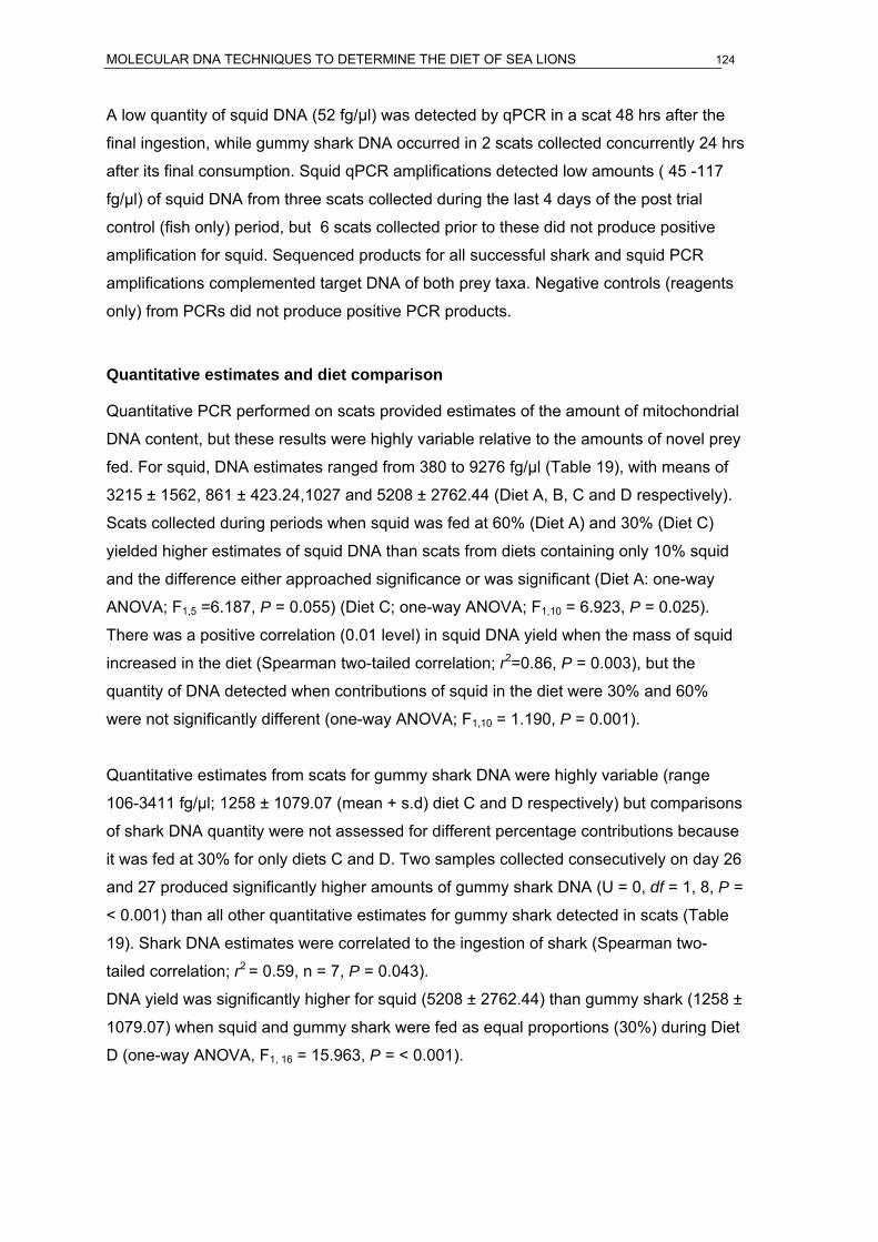
MOLECULAR DNA TECHNIQUES TO DETERMINE THE DIET OF SEA LIONS 124
A low quantity of squid DNA (52 fg/μl) was detected by qPCR in a scat 48 hrs after the
final ingestion, while gummy shark DNA occurred in 2 scats collected concurrently 24 hrs
after its final consumption. Squid qPCR amplifications detected low amounts ( 45 -117
fg/μl) of squid DNA from three scats collected during the last 4 days of the post trial
control (fish only) period, but 6 scats collected prior to these did not produce positive
amplification for squid. Sequenced products for all successful shark and squid PCR
amplifications complemented target DNA of both prey taxa. Negative controls (reagents
only) from PCRs did not produce positive PCR products.
Quantitative estimates and diet comparison
Quantitative PCR performed on scats provided estimates of the amount of mitochondrial
DNA content, but these results were highly variable relative to the amounts of novel prey
fed. For squid, DNA estimates ranged from 380 to 9276 fg/μl (Table 19), with means of
3215 ± 1562, 861 ± 423.24,1027 and 5208 ± 2762.44 (Diet A, B, C and D respectively).
Scats collected during periods when squid was fed at 60% (Diet A) and 30% (Diet C)
yielded higher estimates of squid DNA than scats from diets containing only 10% squid
and the difference either approached significance or was significant (Diet A: one-way
ANOVA; F1,5 =6.187, P = 0.055) (Diet C; one-way ANOVA; F1,10 = 6.923, P = 0.025).
There was a positive correlation (0.01 level) in squid DNA yield when the mass of squid
increased in the diet (Spearman two-tailed correlation; r2=0.86, P = 0.003), but the
quantity of DNA detected when contributions of squid in the diet were 30% and 60%
were not significantly different (one-way ANOVA; F1,10 = 1.190, P = 0.001).
Quantitative estimates from scats for gummy shark DNA were highly variable (range
106-3411 fg/μl; 1258 ± 1079.07 (mean + s.d) diet C and D respectively) but comparisons
of shark DNA quantity were not assessed for different percentage contributions because
it was fed at 30% for only diets C and D. Two samples collected consecutively on day 26
and 27 produced significantly higher amounts of gummy shark DNA (U = 0, df = 1, 8, P =
< 0.001) than all other quantitative estimates for gummy shark detected in scats (Table
19). Shark DNA estimates were correlated to the ingestion of shark (Spearman two-
tailed correlation; r2 = 0.59, n = 7, P = 0.043).
DNA yield was significantly higher for squid (5208 ± 2762.44) than gummy shark (1258 ±
1079.07) when squid and gummy shark were fed as equal proportions (30%) during Diet
D (one-way ANOVA, F1, 16 = 15.963, P = < 0.001).

MOLECULAR DNA TECHNIQUES TO DETERMINE THE DIET OF SEA LIONS 125
Table 18. Total mass ingested (TMI), mass recovered (MR) (wet weight/kg) and percent (%) of mass recovery reconstructed for the total
number of fish recovered (total otoliths recovered divided by 2) from (n) scats for Diet A, B, C, D and controls. Post trial controls were pooled.
Mass estimates were reconstructed from weight length data collected from 100 fresh specimens of each fish species.
Pre control (n =2) Diet A (n =3) Diet B (n= 3) Diet C (n=2) Diet D (n =8) Post control (n =10)
Species t.rough s.perch t.rough s.perch t.rough s.perch t.rough s.perch t.rough s.perch t.rough s.perch
TMI (kg) 12.6 4.2 12.6 4.2 25.2 12.6 18 0 21.6 0 42 42MR (kg) 0 0 0.46 0.18 0 0 0.17 0 0.23 0 0.75 0.45% Recovery 0 0 3.7 4 0 0 <1.0 NA 1.1 NA 1.8 1
* Tommy rough (t.rough)* Striped perch (s.perch)

MOLECULAR DNA TECHNIQUES TO DETERMINE THE DIET OF SEA LIONS 126
(A) Squid (B) Gummy shark
1 2 3 4 5 6 7 8 9 10 11 12 13 14 15 16 17 17 18 19 20 21 22 23 24 25 26 27 28 1 2 3 4 56 7 8 9 10 11 12 13 14 15 16 17 17 18 19 20 21 22 23 24 25 26 27 28 S
1 2 3 4 5 6 7 8 9 10 11 12 13 14 15 16 17 18 19 20 21 22 23 24 25 26 27 28 29 S H
Diet D (30%) Diet B (10%) Diet C (30%) Diet A (60%)
1 2 3 4 5 6 7 8 9 10 11 12 13 14 15 16 17 17 18 19 20 21 22 23 24 25 26 27 28 1 2 3 4 56 7 8 9 10 11 12 13 14 15 16 17 17 18 19 20 21 22 23 24 25 26 27 28 S
1 2 3 4 5 6 7 8 9 10 11 12 13 14 15 16 17 18 19 20 21 22 23 24 25 26 27 28 29 S H
1 2 3 4 5 6 7 8 9 10 11 12 13 14 15 16 17 17 18 19 20 21 22 23 24 25 26 27 28 1 2 3 4 56 7 8 9 10 11 12 13 14 15 16 17 17 18 19 20 21 22 23 24 25 26 27 28 S
1 2 3 4 5 6 7 8 9 10 11 12 13 14 15 16 17 18 19 20 21 22 23 24 25 26 27 28 29 S H
Diet D (30%) Diet B (10%) Diet C (30%) Diet A (60%)
Diet D (30%) Diet C (30%)Diet D (30%) Diet C (30%)
Figure 66. Agarose gel of PCR amplification products showing detection of mtDNA by primers Sepio71c and Gummy71c from DNA recovered
from 28 male faeces. Scats represented by numbers 1-28 were not tested in chronological order of collection, to remove scoring bias. Circled
numbers denote scats collected during each diet week (A = 12, 18 and 22, B = 11 and 17, C = 16, and D = 2, 6, 7, 9, 13, 23, 25, 28) and
numbers in parenthesis are the contribution (% wet weight/kg) of novel prey fed during the 6kg daily diet. Positive controls of target species are
represented by circled S (top plot) and circled G (bottom plot). H indicates negative controls for PCR reaction testing for cross contamination.

MOLECULAR DNA TECHNIQUES TO DETERMINE THE DIET OF SEA LIONS 127
Table 19. PCR amplification results (+) presence (-) absence for standard and real-time
quantitative PCR (qPCR) values (fg/μl) for the detection of squid and gummy shark
mtDNA from scats collected from a captive male ASL during feeding trials at the
Adelaide Zoo. Scat samples represented in chronological order of collection while trial
day (n) indicates actual day of collection for duration of 48 days.
Gummy shark Squid
Diet period Scat No. (trial day) Std. PCR qPCR (fg/µl) Std. PCR qPCR (fg/µl)
Pre control 1 (5) - 0 - 0(0% squid, 0% shark)
Diet A 2 (8) - 1 + 4959(60% squid, 0% shark) 3 (11) - 0 + 3732
4 (12) - 0 + 1232
Diet B 5 (14) - 8 + 2938(10% squid, 0% shark) 6 (16) - 3 + 380
7 (18) - 3 + 1177
Diet C 8 (20) - 2 - 1027(10% squid, 30% shark) 9 (26) + 3411 + 1129
Diet D 10 (27) + 2072 + 1746(30% squid, 30% shark) 11 (29) + 409 + 9276
12 (29) + 1062 + 407913 (29) + 1532 + 425414 (30) + 360 + 547415 (30) + 466 + 796516 (33) - 106 + 528917 (33) + 1907 + 7659
Post control 18 (35) - 3 - 52(0% squid, 0% shark) 19 (36) - 1 - 0
20 (37) - 1 - 021 (38) - 1 - 022 (39) - 2 - 023 (40) - 1 - 024 (41) - 11 - 625 (43) - 1 - 4526 (46) - 0 - 11727 (47) - 0 - 5728 (48) - 0 - 0

MOLECULAR DNA TECHNIQUES TO DETERMINE THE DIET OF SEA LIONS 128
Discussion
Morphological assessment of hard-prey remains
Morphological identification of undigested prey remains recovered from dietary samples
is a widely used and effective method to assess the diet of many marine predators,
including fish (Cortés, 1997; Cortés 2000; Simpendorfer et al. 2001), seabirds (Gales
and Pemberton, 1990; Cullen et al. 1992; Clausen and Putz, 2002) and seals (Gales et
al.1993; Gales and Pemberton, 1994; Goldsworthy et al. 1997; Page et al. 2005). Most
studies based on this methodology are constrained by the probability that the recovery of
the prey remains is biased toward prey species with robust skeletal structures. This
method may underestimate the consumption of soft bodied species and species with
reduced digestive resistance (Harvey, 1989; Fea and Harcourt, 1997; Lalas, 1997;
Needham, 1997; Orr and Harvey, 2001; Staniland, 2002; de Bruyn et al. 2003; Deagle et
al. 2005b). Studies that identify prey remains from faeces incorporate these inherent
biases, but the method remains a simple non-intrusive means of obtaining large
quantities of dietary information. Morphological analysis of captive ASL scats identified very few of the prey ingested and
was limited to the robust diagnostic remains of the fish. Otolith recovery in scats
collected from the experimental male was highly variable (1-22 per scat), and because
identifiable fish remains were limited, their relative importance in the captive diet was
highly underestimated. Given that otolith recovery rates were not related to the number
of fish per species fed or otolith size ingested, the higher occurrence of tommy rough
otoliths in scats collected from the male may be explained by inter-specific differences in
the digestibility of the fish which can result in under or overestimates of the prey
consumed (Jobling, 1987; Cotrell et al.1996; Tollit et al. 2003). Hard-prey analysis did
not however, produce quantitative information of the fish ingested by the control female
sea lion, even though a mixed diet of 3337 fish were fed over the duration of the trial.
Low otolith recovery rates in captive male and female ASL fed integrated diets were
noted by Gales and Cheal (1992), who also highlighted the potential for individual and/or
sex-specific biases in the recovery of cephalopod remains from scats. Similar to their
study, otolith recovery rates from this study were lower for the female (0.0001%) than the
male (2%) but a disparity was shown between the recovery rates of cephalopod remains
in scats from male (9%) and female (98%) sea lions. This contrasts our study, as
morphological analysis did not recover squid beaks even when they were the
MOLECULAR DNA TECHNIQUES TO DETERMINE THE DIET OF SEA LIONS 129
predominant prey species by mass in the diet of the male. Even though outputs of
cephalopod remains are highly variable between captive otariids (Tollit et al. 1997; Orr
and Harvey, 2001), this study is the only otariid captive diet study we are aware of that
has not recovered cephalopod beaks from a feeding trial. Similar extremes in low
recovery of prey remains observed in captive otariids have also been documented by
Casper (2007b) for A. forsteri and A. tropicalis and Gales and Cheal (1992) for N.
cinerea.
The low recovery of squid beaks in scats may be explained as a function of gastric
retention whereby larger cephalopod beaks are retained within the stomach through an
inability to pass through the narrow pyloric region, into the small intestine and lower
colon (Richardson and Gales, 1987) or alternatively, remains are destroyed in the
stomach by the presence of gastric stones (Needham, 1997). Stomach and regurgitate
diet analysis studies on ASL support this theory as they have shown that cephalopod
hard parts, among other larger hard prey remains are retained within the stomach
(McIntosh et al. 2006b, Gales and Cheal 1992). Gales and Cheal (1992) indicated that
the probability of recovering cephalopod beaks from the scats of captive ASL was related
to their size; larger beaks were absent in female scats and few (9-16%) were present in
scats of the male. Consistent with this trend observed in many wild otariid seals and
highlighted in free living ASL by McIntosh et al. (2006), it is reasonable to suggest that
the absence of cephalopod beaks in scats collected from this study were likely retained
within the stomach of the adult male, as we found no evidence over the duration of the
trial of any egested beaks in the single regurgitate or scats.
The marked differences of hard prey recovery of fish remains between male and female
ASL in our study may be related to the differences observed in the activity levels of the
two animals. Tollit et al. (2003) observed periods of inactivity in captive fed Steller sea
lions (Eumetopias jubatus) resulted in long retention rates of fish prey remains, while
physical activity induced faster excretion. Similarly, Helm (1984) found that captive fed
pinnipeds defecated during higher levels of activity such as swimming, while Dellinger
and Trillmich (1987) recovered fewer experimental beads fed to sea lions prior to events
of swimming than periods of confinement. This study observed a high level of activity by
the male; each day consisted of continual swimming in a large deep pool, while the
female was primarily inactive. Even though the number of scats collected from male and
female was similar, elevated activity by the male may have generated higher otolith
recovery rates by stimulating the movement of digesta through the gastrointestinal tract
that facilitated the faster voiding of prey remains. Because prey digestion occurs
predominantly in the stomach of pinnipeds (Frost and Lowry, 1980) inactivity of the

MOLECULAR DNA TECHNIQUES TO DETERMINE THE DIET OF SEA LIONS 130
female possibly induced a higher level of digestion whereby skeletal structures were
exposed to gastric acids for longer periods than the male accounting for their absence in
the scat samples.
If our morphological analysis provided the primary source of evidence to infer diet about
ASL from this captive study, it would be interpreted that captive sea lions from these
trials consume limited number of tommy rough and striped perch and do not consume
squid or gummy shark. Even though discrepancies were found in our morphological
analysis, this method does provide some qualitative data of the prey species consumed.
However, because prey consumption by free foraging seals does not guarantee that
identifiable remains are consumed, care must be taken when applying this dietary
assessment technique to wild ASL scats as the biases exhibited in this study can impose
significant implications when interpreting prey frequency and abundance from dietary
remains.
DNA assessment of diet – Standard PCR and quantitative PCR
This is the first study to assess the suitability of molecular based DNA analysis on scats
collected from ASL. This study has shown that DNA analysis is the most reliable of the
two methods tested, in detecting the presence of specific prey species that would
otherwise not have been detected using morphological analysis.
Our DNA analysis was based on the mitochondrial DNA detection of squid and shark
novel prey species consumed in the diet by captive adult male ASL. Molecular DNA-
based analysis detected and quantified the relative proportions of each novel prey
species from scats, when hard remains were completely absent.
The results from our PCR experiments suggest that DNA extracted from ASL scats was
highly degraded because we could not detect DNA from prey unless short DNA
sequences were targeted of less than 100 base pairs in size. We tested a number of
target sequences >100bp in length for each novel prey and fish prey taxa on scats, and
although we found no flexibility in the robustness of the DNA quality or DNA fragment
target size, we believe that detection is reliable as even prey biomass at 10% of the diet
could be detected. Casper et al. (2007) noted similar results to our study, but used
nested PCR DNA-based detection to identify prey in scats from captive sub-Antarctic
and New Zealand fur seals fed integrated diets. They surmised that by targeting smaller
fragments of prey DNA (100bp) in a matrix of low quality DNA template may have

MOLECULAR DNA TECHNIQUES TO DETERMINE THE DIET OF SEA LIONS 131
contributed to their higher detection rates of squid DNA from scats, while larger target
DNA fragments of 200 bp were less successful. Frantzen et al. (1998) has also shown
from their DNA-based faecal diet study on primates that success of PCR amplification is
likely to increase with a decrease in target product size using short DNA sequences
(100-200bp) because longer DNA fragments are less likely to survive the digestive
process. Other studies using molecular DNA-based assessments of diet have utilised
small product sizes to target prey DNA in faeces (Kohn et al. 1995; Farrell et al. 2000;
Jarman et al. 2002; Purcell et al. 2004; Deagle et al. 2005b; Casper et al. 2007b), but in
contrast to these, our study and one other DNA diet assessment of wild Antarctic fur
seals scats by Casper et al. (2007a) have targeted prey sequences less than 100 bp.
Using larger DNA target sequences for faecal diet assessment could lead to substantial
differences in the frequency of detection of important prey species DNA using these
methods given that DNA template quantity and quality is likely to be compromised
(Taberlet et al. 1999).
Qualitative DNA assessments using standard or quantitative PCR to determine the initial
detection time or day of origin of the novel prey DNA being detected was unclear for
each prey species because scats were produced sporadically and our sample size was
relatively small. Initial detection time of shark DNA was constrained by the absence of
scats during the first week after its introduction into the diet while squid was only
detected ~24-36hrs after its initial ingestion because samples were not produced for the
first two days following its introduction. These estimates of initial detection time were also
proximal because of the limited access to scats overnight. Given that both our PCR
assays were highly sensitive and could detect extremely low quantities of gummy shark
(2 fg/μl) and squid (20 fg/μl) DNA, the final detection times could not determine the day
of origin for the prey DNA being detected but could determine how long prey persist in
the gut.
We did find that detection success rates for squid and shark decreased rapidly after the
final ingestion of either species which supports the rapid passage rates documented for
ASL (Richardson and Gales, 1987; Bodley et al. 1997). Our results demonstrate that
successful DNA detection is limited to a maximum of 48hrs after the final ingestion after
which the quantity and potential quality of prey DNA become significantly reduced or
absent. No scats were collected the day following the final ingestion of either novel prey,
so estimates of the rate which larger amounts of prey DNA persist in the digestive tract
of ASL remains unclear. Our final DNA detection times of squid were similar to other
otariid faecal DNA studies using these techniques. Casper et al. (2007a) found that DNA
MOLECULAR DNA TECHNIQUES TO DETERMINE THE DIET OF SEA LIONS 132
detection of squid was limited to a maximum of 32hrs after the final prey ingestion by
captive sub-Antarctic (A. tropicalis) and New Zealand (A. forsteri) fur seals, while Deagle
et al. (2005) used quantitative PCR and detected prey DNA 48hrs after prey was fed to
captive Steller sea lions. Two possible explanations for these results are that 1) prey
DNA is voided rapidly in active ASL, or 2) DNA within the gut degrades rapidly so that
DNA detection after defecation is highly reduced. This has significant implications when
samples are collected from wild ASL colonies, as DNA extracted from scats may only
represent the most recent days of prey ingestion rather than prey consumed over
foraging trips distant from the colony.
The detection of small proportions of squid DNA (45-117 fg/μl) in 3 scats on conclusion
of our trial may lend support to the elevated stomach retention rates of prey observed in
pinnipeds. Even if all remains were voided from the small intestine from the adult male,
remnant DNA from remains trapped and broken down in the stomach have the potential
to be detected weeks later. This hypothesis is plausible, given that ASL have shown high
retention of larger prey remains within their stomachs and squid beaks from our
morphological analysis from this study were absent.
We compared the application of standard and real-time quantitative PCR to determine
whether detection success of prey DNA from scats would be significantly different.
Because small amounts of target DNA from scats cannot always be detected using
standard PCR methodologies, fluorescent markers such as SYBR green can increase
the detection rate, and generate a quantitative value for the relative amounts of DNA
present in each sample. Quantitative PCR assessment of DNA from scats was a more
reliable DNA detection method than standard PCR because it produced a higher DNA
detection success rate in all scats containing the novel prey, and could detect some prey
DNA 48hrs after its final ingestion where standard PCR could not. Standard PCR
success rates were 88% for shark and 89% for squid, with at least one PCR assay for
each primer not detecting either prey species within a scat collected during the
experimental diets. Detection was limited by poor visualisation of the PCR products or
low estimates of dsDNA, most likely as a result of the surprisingly low levels of amplified
DNA in each scat even after PCR amplification. This may suggest that our initial DNA
template prior to PCR was in extremely poor condition which could be attributable to the
digestive processes of ASL.
We assessed quantifying novel prey DNA to determine if the relative amounts of prey
recovered in faeces were proportional to their mass contribution in the diet. Quantitative

MOLECULAR DNA TECHNIQUES TO DETERMINE THE DIET OF SEA LIONS 133
PCR is useful for determining prey contributions in pinniped diet studies when
identification of hard-parts is ambiguous (Deagle et al. 2005; Deagle et al. 2007). In our
study, all scats containing DNA from novel prey were quantifiable, but the relative
amount of DNA varied markedly for each prey species between all scats. Scats that were
collected within the same experimental diet also showed significant differences, but
these results are not surprising given that digestion and subsequent voiding of prey is
not uniform. Nevertheless, if the amount of novel prey DNA detected in scats could be
directly attributable to each diet, when scat qPCR measurements were pooled for each
diet, larger contributions by mass of squid (60%, 30%) consistently produced higher DNA
estimates, which were statistically different from lower DNA estimates produced from
scats when the diet contained small mass contributions of squid. We did observe that
DNA content increased in scats when the consumption of the novel prey species
increased, but the relationship for shark was weaker than squid primarily because shark
was only fed at one mass contribution throughout the trial and the number of scats
collected after its initial ingestion became highly infrequent.
Our qPCR values did not indicate a difference between the two higher consumption rates
of squid in the diet, but this may have also resulted from the low number of replicates of
scat samples collected when squid was fed at it highest mass contribution at the
beginning of the trial. Our DNA estimates are consistent with the results from DNA
recovered and quantified from captive Steller sea lion scats as noted by Deagle and
Tollit (2007). The quantification of prey DNA from faeces collected from their captive
study also showed massive variation in DNA copy number between 3 fish species fed,
even when prey contributions remained constant throughout their feeding trial. They
suggested that prey specific DNA-biases associated with DNA survival were a
contributing factor affecting DNA recovery, which may overestimate or underestimate
actual importance of prey taxa in the diet.
Our quantitative estimates did show significant higher amounts of DNA recovered for
squid than shark when fed in equal proportions by mass in the diet. This difference was
not likely a result of our primers targeting different prey DNA fragment size as we
removed this bias by designing primers to detect identical sequence lengths for each
novel species. Alternatively, even though increased PCR amplification success rates can
sometimes remain unexplained, the elevated yield of squid DNA may not be explained
by the PCR efficiency rates, as qPCR efficiency for detecting and quantifying gummy
shark DNA was 10% higher than squid. These differences may be explained in relation
to the concentration of DNA in the different tissue types represented by each of the novel

MOLECULAR DNA TECHNIQUES TO DETERMINE THE DIET OF SEA LIONS 134
prey species, the ability of each tissue’s cells and DNA to survive the digestive process
or a combination of both. Cephalopods generally exhibit hyperplasic exponential tissue
growth over a short life span compared to elasmobranchs that demonstrate slow growth
rates and size plateaus at maturity (Moltschaniwskyj, 1994; Cortes, 2000; Frisk et al.
2001,). Given that whole squid containing a diverse range of tissue was fed compared to
only the muscle tissue of mature shark could increase the likelihood of detecting larger
amounts of DNA if more DNA is present. Our prey tissue DNA extractions used for
positive controls did yield significantly higher concentrations of squid DNA than shark
DNA from the initial tissue samples. These differences are noteworthy given that Deagle
and Tollit (2007) also found considerable differences in the relative proportions of DNA in
prey tissues when compared to mass proportions. These potential biases require further
investigation.
Conclusions
The application of molecular DNA assessment of scats, collected from captive ASL is an
effective method to identify ingested prey taxa, even when hard remains are not present
in scats. For wild ASL colonies, this will be useful technology as preliminary
morphological analysis of scats from some colonies has revealed limited representation
of diagnostic skeletal structures which has hindered the taxonomic identification of the
important prey in the diet. The sensitivity of quantitative PCR assessment has the
advantage of detecting minimal quantities of target DNA in faecal samples that otherwise
may not be detected by standard PCR, but these outcomes are highly dependant on the
quality of DNA template and the size of the target DNA sequences.
Furthermore, prior knowledge of key taxonomic groups and species such as those data
from traditional diet analysis techniques will provide greater resolution for the potential
prey targets of DNA analysis, which otherwise would be difficult to target and time costly
if DNA-based methodologies are used alone. Molecular DNA techniques provide further
insight into information on dietary preferences and trophic relationships. For ASL its
application deserves further investigation, because the consumption of the major prey
species can be determined using this non-invasive approach.
RECOMMENDATIONS FOR FURTHER RESEARCH 135
RECOMMENDATIONS FOR FURTHER RESEARCH
As detailed in previous sections, results from the risk assessment clearly demonstrate
that the potential risk to ASL from bycatch in the gillnet sector of the SESSF and the
SARLF are significant and needs to be mitigated.
Spatial management options could be investigated to assess how effort and catch could
be reallocated to reduce the impact of bycatch on high-risk ASL subpopulations.
Enhanced spatial tools for risk assessment will be required if spatial management of
fishing effort is to become a management strategy for mitigating ASL bycatch in the
demersal gillnet fishery. Further development of such tools are required, because current
models are limited by the absence of data on the foraging movements of sea lions in
some high-risk regions, as well as the absence of accurate fishing effort data. Further
satellite tracking of ASL at subpopulations identified as high-risk should be undertaken to
improve the accuracy of spatial foraging models.
In 2006, demersal gillnet fishers were required to record the latitude/longitude positions
of each net-set, and from July 2007, all vessels will be fitted with satellite-linked vessel
monitoring systems that will significantly improve the resolution of fishing effort.
Following improvements of these data sets, it is recommended that bycatch probabilities
be re-estimated and used to model the benefits of different spatial-management
scenarios that could include area-closures, and reductions or redistributions of fishing
effort. Improved fishery observer coverage will be essential to provide real estimates of
bycatch rates and support for spatial-closures in regions of high-risk. They will also be
essential to provide ongoing performance measures to managers about the
effectiveness of spatial management approaches adopted in reducing bycatch to
sustainable levels, and ensuring it does not threaten the viability of any subpopulation.
Ongoing abundance estimates of ASL subpopulations will be the critical performance
measure of spatial management in the fishery.
This study demonstrates the feasibility of quantifying prey DNA in the faeces of ASL and
provides an assessment of using this data to obtain quantitative diet composition data.

BENEFITS AND ADOPTION 136
BENEFITS AND ADOPTION
The benefits of adopting the recommendations detailed in this report and in supporting
future research will be:
• the development of, and industry and management adoption of mitigation options
to reduce seal bycatch in both the SARLF and gillnet sector of the SESSF
• addressing the outstanding ESD recommendations detailed in fishery ESD
assessments
• mitigation of the key threatening process identified in the ASL Draft Recovery
Plan
• recovery of the ASL, and potential future delisting of the species as Threatened.
The major beneficiaries will be the gillnet sector SESSF and SARLF, natural resources
managers (PIRSA Fisheries, AFMA, Commonwealth DEH, SA DEH), fisheries and
marine mammal biologists and the Australian community. All will benefit from the
knowledge of the significance and role of fishery bycatch on seal populations.
Furthermore, future development of the recommendations will assist in:
• implementing ESD objectives in the southern rock lobster and southern shark
fisheries
• environmental accreditation to enhance market opportunities for the fisheries,
• the recovery of the ASL and
• achieving benchmarks in ecosystem-based fisheries management.
The use of genetic analysis of faeces for studying the diet of ASL allows assessment of
potential biases from traditional approaches. DNA analyses can also provide improved
taxonomic identification of prey and can be used to address questions beyond the scope
of traditional methods of diet analysis. Such information is required to understand their
key prey species, habitats and trophic interactions with fisheries.
LITERATURE CITED 137
FURTHER DEVELOPMENT
An FRDC proposal developed from the findings of the pilot study has recently been
approved for funding (2007/041). It will form a comprehensive research and development
program to develop mitigation options to manage seal bycatch issues in the SARLF and
gillnet SESSF.
The proposal was developed with extensive stakeholder consultation. Findings of the
pilot study, a report to FRDC (Goldsworthy and Page 2007) and the objectives and
details of the aims of the FRDC project being developed were presented to both the
southern and northern zone FMCs of the SARLF, and to the GHATMAC. Ongoing
consultation is progressing with PIRSA Fisheries, AFMA, Commonwealth and SA DEH
and SharkRAG.
Assessment of the presence/absence and importance of several commercially-fished
species in the diets of wild ASL has commenced using faecal/enema samples obtained
from a range of colonies and South and Western Australia.
REFERENCES
Akçakaya, H.R (1998) RAMAS Metapop: Viability Analysis for Stage-structured
Metapopulations (version 3.0). Applied Biomathematics, Setauket, New York
Alava, J.J., and Salazar, S. (2006) Status and Conservation of Otariids in Ecuador and
the Galápagos Islands. pp 495-519. In ‘Sea Lions of the World’. (Eds A. W.
Trites, S. K. Atkinson, D. P. DeMaster, L. W. Fritz, T. S. Gelatt, L. D. Rea and K.
M. Wynne). Alaska Sea Grant College Program, University of Alaska: Fairbanks,
Alaska.
Albaugh, G.P., Iyengar, V., Lohani, A., Malayeri, M., Bala, S., and Nair, P.P. (1992).
Isolation of exfoliated colonic epithelial cells, a novel non-invasive approach to
the study of cellular markers. International Journal of Cancer. 52(3): 347-350.
Alonso, M.A., Crespo, E.A. and Pedraza, S.P. (2000). Food habits of the South
American sea lion, Otaria flavescens, off Patagonia, Argentina. Fisheries
Bulletin98:250-263
Altschul, S.F., Gish, W., Miller, W., Myers, E.W, and Lipman, D.J.(1997) Basic local
alignment search tool. Journal of Molecular Biology. 215: 403-410.

LITERATURE CITED 138
Anderson, S.M., Lyndersen, C., Grahl-Neilson, O., and Kovacs, K.M. (2004). Autumn
diet of harbour seals (Phoca vitulina) at Prins Karls Forland, Svalbard, assessed
via scat and fatty acid analyses. Canadian Journal of Zoology 82: 1230-1245.
Barlow J and Boveng P (1991) Modeling age-specific mortality for marine mammals.
Marine Mammal Science 71:50-65.
Birky, C.W., Fuerst, P., and Maruyma, T.(1989). Organelle gene diversity under
migration, mutation and drift: equilibrium exceptions, approach to equilibrium,
effects of heteroplasmic cells, and comparison to nuclear genes. Genetics. 121:
613-627.
Bodley, K.B., Mercer, J. R., and Bryden, M. M. (1999). Rate of passage of digesta
through the alimentary tract of the New Zealand fur seal (Arctocephalus forsteri)
and the Australian sea lion (Neophoca cinerea) (Carnivora : Otariidae). Australian
Journal of Zoology. 47: 193-198.
Bowen W.D. (2000) Reconstruction of pinniped diets: accounting for complete digestion
of otoliths and cephalopod beaks. Canadian Journal of Fisheries and Aquatic
Research. 57: 898-905. et al. 1994;
Boyd IL, Croxall JP, Lunn NJ, and Reid K. (1995) Population demography of Antarctic fur
seals: the costs of reproduction and implications for life histories. Journal of
Animal Ecology 64: 505-518
Boyle P.R., Pierce, G.J., Diack, J.S.W. (1991). Sources of evidence for salmon in the
diets of seals. Fisheries research. 10: 137-150.
Campbell, R. (2003) Demography and population genetic structure of the Australian sea
lion, Neophoca cinerea. PhD thesis. University of Western Australia, Western
Australia. 153pp (including appendices).
Campbell, R. (2004). Report for the Sea Lion Scientific Reference Group. Fisheries
Occasional Paper No. 16. Department of Fisheries, Government of Western
Australia. 20pp, plus references and appendices.
Campbell R, Chubb C, Webster F and Weir K (2004) Ecosystem-based management of
the fishery for the western rock lobster, Panulirus cygnus, with special reference
to interaction with Australian sea lion. Abstract: 7th International Conference and
Workshop on Lobster biology and management. 8-13 February 2004, Hobart.
Campbell, R. (2005). Historical distribution and abundance of the Australian sea lion
(Neophoca cinerea) on the west coast of Western Australia. Fisheries Research
Report No. 148. Department of Fisheries, Government of Western Australia.
42pp.

LITERATURE CITED 139
Carretta, J.V., K.A. Forney, M.M. Muto, J. Barlow, J. Baker, and M. Lowry. (2004) U.S.
Pacific marine mammal stock assessments. pp 5-11. NOAA-TM-NMFS-SWFSC-
358 Tech. Memo. 295 pp.
Casaux, R., Baroni, A., Arrighetti, F., Ramon, A. and Carlini, A. (2003). Geographical
variation in the diet of the Antarctic fur seal Arctocephalus gazella. Polar biology
26: 753-758.
Casper, R.M., Jarman, S.N., Gales, N.J., and Hindell, M.A. (2007a). Combining DNA and
morphological analyses of faecal samples improves insight into trophic
interactions: a case study using a generalist predator. Marine Biology.
DOI10.1007/s00227-007-0732-y
Casper, R.M., Jarman, S.N., Deagle, B.E., Gales, N.J., and Hindell, M.A. (2007b).
Detecting prey from DNA in predator scats: A comparison with morphological
analysis, using Arctocephalus seals fed a known diet. Journal of Experimental
Biology and Ecology. 347: 144-154.
Caughley G (1977) Analysis of vertebrate populations. John Wiley and Sons, Chichester
Childerhouse, S., Dix, B., and Gales, N. (2001) Diet of New Zealand sea lions
(Phocarctos hookeri) at the Auckland Islands. Wildlife Research 28:291-298.
Clausen, A.P., and Pütz, K. (2002). Recent trends in diet composition and productivity of
Gentoo, Magellanic, and Rockhopper penguins in the Falkland Islands. Aquatic
Conservation : Marine and Freshwater Ecosystems. 12: 51-61.
Cottrell, P.E., Trites, A.W., Miller, E.H. (1996). Assessing the use of hard parts in faeces
to identify harbour seal prey: results of captive feeding trials. Canadian Journal of
Zoology.74: 875-880.
Cortés Enric (2000). Life history patterns and correlations in sharks. Reviews in Fisheries
Science.8(4): 299-344.
Cortés, E., and Gruber, S.H (1997). Diet, feeding habits and estimates of daily ration of
young lemon sharks Negaprion brevirostris (Poey). Copeia, Vol. 1990, No. 1
(Mar. 6, 1990), 204-218.
Crespo, E.A., and Pedraza, S.N. (1991) Estado actual y tendencia de la poblacion de
lobos marinos de un pelo (Otaria flavescens) en el litoral norpatagonico
(Spanish). Ecologia Austral 1: 87–95.
Cullen, J.M., Montague, T.L., and Hull, C.(1992) Food of little penguins Eudyptula minor
in Victoria: Comparison of three localities between 1985 and 1988.EMU. 91: 318-
341.
De Bruyn, P.J.N., Bester, M.N., Mercenero, S., Kirkman, S.P., Roux, J-P., and Klages
N.T.W. (2003). Temporal variation of cephalopods in the diet of cape fur seals in
Namibia. South African Journal of Wildlife Research.3392): 85-96.

LITERATURE CITED 140
Deagle B. E., Tollit D.J., Jarman S.N., Hindell, M.A., Trites, A.W., and Gales N.J.
(2005a). Molecular scatology as a tool to study diet: analysis of prey DNA in
scats from captive Steller sea lions. Molecular Ecology 14: 1831-1842.
Deagle B. E., Jarman S.N., Pemberton, D., and Gales, N.J.(2005b). Genetic screening of
prey in the gut contents from a giant squid (Architeuthis sp). Journal of Heredity
96: 417-423.
Deagle, B.E., Eveson, J.P., and Jarman, S.N.(2006). Quantification of damage in DNA
recovered from highly degraded samples- a case study on DNA in faeces.
Frontiers in Zoology. 3: (11)1-10.
Deagle, B.E., and Tollit, D.J. (2007). Quantitative analysis of prey DNA in pinniped
faeces: potential to estimate diet composition? Conservation Genetics. 8: 743-
747.
Dellinger, T., and Trillmich, F. (1987). Estimating diet composition from scat analysis in
otariid seals (Otariidae): is it reliable? Canadian Journal of Zoology. 66: 1865-
1870.
Dennis TE and Shaughnessy PD (1996) Status of the Australian sea lion, Neophoca
cinerea, in the Great Australian Bight region of Western Australia. Wildlife
Research, 26: 383-388.
Department of the Environment and Heritage (2003a). Assessment of the Southern and
Eastern Scalefish and Shark Fishery. Department of the Environment and
Heritage (Commonwealth DEH) report to the Minister for the Environment and
Heritage, September, 2003. 79pp.
Department of the Environment and Heritage (2003b). Assessment of the South
Australian Rock Lobster Fishery. Department of the Environment and Heritage
(Commonwealth DEH) report to the Minister for the Environment and Heritage,
October, 2003. 34pp.
Ellner, S.P, Fieberg, J., Ludwig, D., and Wilcox, C. (2002) Precision of population
viability analysis. Conservation Biology. 16:258-261.
Farrell, L., Roamn, J., and Sunquist, M.E (2000). Dietary separation of sympatric
carnivores identified by molecular analysis of scats. Molecular Ecology. 9: 1583-
1590.
Fea, N.I., and Harcourt, R. (1997). Assessing the use of faecal and regurgitate analysis
as a means of determining diet of New Zealand fur seals. In Marine mammal
research in the southern hemisphere (Ed. M. Hindell and C. Kemper), pp143-150.
Chipping Norton, Australia: Surrey Beatty & Sons Pty. Ltd.

LITERATURE CITED 141
Fea, N.I., and Harcourt, R. and Lalas, C. (1999).Seasonal variation in the diet of New
Zealand fur seals(Arctocephalus forsteri) at Otago Peninsula, New Zealand.
Wildlife Research 26: 147-160.
Fletcher, W. J., Chesson, J., Sainsbury, K. J., Hundloe, T., Smith, A. D. M., and
Whitworth, B. (2002). National ESD reporting Framework for Australian Fisheries:
The “How to Guide for Wild Capture Fisheries” FRDC report 2000/145, Canberra,
Australia.
Fowler, C.W. (1987) Marine debris and northern fur seals: a case study. Marine Pollution
Bulletin. 68:326-335.
Fowler, C.W., Merric, R., and Baker, J.D. (1990). Studies of the population level effects
of entanglement on northern fur seals. In: Shormura, R.S., and Godfrey, M.L.
(eds.). Proceedings of the International Conference on Marine Debris, Honolulu.
NOAA Technical Memo. 453-474.
Frantzen, M.A.J., Silk, J.B., Ferguson, J.W.H., Wayne, R.K., and Kohn, M.H. (1998).
Empirical evaluation of preservation methods for faecal DNA. Molecular
Ecology.7: 1423-1428.
Frisk, M.G., Miller,T. J., and Fogarty, M.J. (2001). Estimation and analysis of biological
parameters in elasmobranch fishes:a comparative life history study. Canadian
Journal of Fisheries and Aquatic Science. 58: 969-981.
Frost, K.J., and Lowry, L.F. (1980). Feeding of the ribbon seal(Phoca fasciata) in the
Bering Sea in spring. Canadian journal of Zoology. 58:1601-1607.
Gales, N. J., and Cheal, A.J. (1992). Estimating diet composition of the Australian sea
lion (Neophoca cinerea) from scat analysis: an unreliable technique. Wildlife
Research 19: 447-456.
Gales, N. J., Shaughnessy, P. D., and Dennis, T. E. (1994) Distribution, abundance and
breeding cycle of the Australian sea lion Neophoca cinerea (Mammalia:
Pinnipedia). Journal of Zoology, London 234, 353-370.
Gales, N. J. and Costa, D.P. (1997) The Australian sea lion, a review of an unusual life
history. In: Hindell, M., Kemper, C. (eds.). Marine mammal research in the
Southern Hemisphere, Vol. 1 Status, ecology and medicine. Surrey Beatty and
Sons, Chipping Norton. pp. 78-87.
Gales, R., and Pemberton, D. (1990) Seasonal and local variation in the diet of the little
penguin, Endyptula minor, in Tasmania. Australian Wildlife Research. 17: 231-59.
Gales, R., Pemberton, D., Lu, C., and Clarke, M.R.(1993). Cephalopod diet of the
Australian fur seal: variation due to location, season and sample type. Australian
journal of Marine and Freshwater Research 44: 657-671.

LITERATURE CITED 142
Gales, R., and Pemberton, D. (1994). Diet of Australian fur seals. Australian Journal of
Marine and Freshwater Research 45: 653-664.
Gilpin, M.E. and Soulé, M.E. (1986) Minimum viable populations: processes of species
extinction. In: ME Soulé (ed) Conservation Biology: the science of scarcity and
diversity, Sinauer Associates, Sunderland, Massachussets. pp 19-34.
Goldsworthy, S. D., Hindell, M. A. and Crowley, H. M. (1997). Diet and diving behaviour
of sympatric fur seals Arctocephalus gazella and A. tropicalis at Macquarie
Island. In Marine mammal research in the Southern Hemisphere. Hindell, M. and
Kemper, C. (eds). Surrey Beatty and Sons: Chipping Norton, Sydney, pp.151-
163.
Goldsworthy SD, Bulman C, He X, Larcombe J, and Littnan C (2003) Trophic
interactions between marine mammals and Australian fisheries: an ecosystem
approach. In: Gales N, Hindell M, and Kirkwood R. (eds) Marine Mammals and
Humans: Fisheries, tourism and management. CSIRO Publications. pp 65-99
Goldsworthy SD, Shaughnessy PD, Page B, Hamer D, Peters K, and McIntosh R (2005)
PIRSA Aquaculture/FRDC - Innovative solutions for Aquaculture planning and
management: addressing seal interactions in the finfish aquaculture industry.
Milestone Progress Report to the Fisheries Research Development Corporation.
FRDC project number 2004/201. 97pp.
Goldsworthy SD and Page B (2007) Risk-assessment of seal interactions in the South
Australian rock lobster and gill-net sector of the southern and eastern scalefish
and shark fishery. In Goldsworthy SD, Hamer and Page B (eds) Assessment of
the implications of interactions between fur seals and sea lions and the southern
rock lobster and gillnet sector of the Southern and Eastern Scalefish and Shark
Fishery (SESSF) in South Australia. Final Report to the Fisheries Research and
Development Corporation. South Australian Research and Development Institute
(Aquatic Sciences), Adelaide, 164 pp. SARDI Publication no. F2007/000711-1.
Hall, M.A. (1996). Strategic issues in managing fisheries bycatch. In: Hall, M.A. (ed.).
Solving bycatch: considerations for today and tomorrow. University of Alaska Sea
Grant College Program, Fairbanks. Report number: 96-03.
Hamer D (2007) Synthesise and review the fishery logbooks for the SA rocklobster and
gillnet sector SESSF fisheries for reports of interactions with seals. In
Goldsworthy SD, Hamer and Page B (eds) Assessment of the implications of
interactions between fur seals and sea lions and the southern rock lobster and
gillnet sector of the Southern and Eastern Scalefish and Shark Fishery (SESSF)
in South Australia. Final Report to the Fisheries Research and Development

LITERATURE CITED 143
Corporation. South Australian Research and Development Institute (Aquatic
Sciences), Adelaide, 164 pp. SARDI Publication no. F2007/000711-1.
Harvey, J.T. (1989). Assessment of errors associated with harbor seals (Phoca vitulina)
faecal sampling. Journal of Zoology (London) 247: 177-181.
Harwood J, and Prime JH (1978) Some factors affecting the size of British grey seal
populations. Journal of Applied Ecology 15:401-11.
Helm, R.C. (1984).Rate of digestion in three species of pinnipeds. Canadian journal of
Zoology. 62: 1751-1756.
Higgins, LV., and Gass, L. (1993) Birth to weaning: parturition, duration of lactation, and
attendance cycles of Australian sea lions (Neophoca cinerea). Canadian Journal
of Zoology. 71:2047-2055.
Hood, G. M. (2006). Poptools version 2.7.5. URL. http://www.cse.csiro.au/poptools.
Hume, F., Hindell, M.A., Pemberton, D., and Gales, R. (2004). Spatial and temporal
variation in the diet of a high trophic level predator, the Australian fur seal
(Arctocephalus pusillus doriferus). Marine Biology. 144: 407-415.
Hyslop, E.J. (1980). Stomach contents analysis- a review of their methods and their
application. Journal of Fish Biology. 17: 411-429.
Jarman, S.N., Gales, N.J., Tierney M., Gill, P.C., and Elliott, N.G.(2002). A DNA-based
method for identification of krill species and its application to analysing the diet of
marine vertebrate predators. Molecular ecology 11: 2679-2690.
Jarman, S.N., Redd, K.S., gales, N.J. (2006). Group specific primers for amplifying DNA
sequences that identify Amphipoda, Cephalopoda, Echinodermata, Gastropoda,
Isopoda, Ostracoda and Thoracia. Molecular Ecology. 6: 268-271.
Jobling, M. (1987). Marine mammal faeces samples as indicators of prey importance; a
source of errorin bioenergetics studies. Sarsia. 265-274.
Kohn, M., Knauer, F., Stofella, A., Schroder, W., and Paabo, S (1995). Conservation
genetics of the European brown bear- a study using excremental PCR of nuclear
and mitochondrial sequences. Molecular Ecology. 4: 95-103.
Lalas, C. (1997). Prey of Hooker's sea lions Phocarctos hookeri based at Otago
Peninsula new Zealand. In 'Marine Mammal Research in the Southern
Hemisphere. Vol 1: Status, Ecology and Medicine'. (eds M.A Hindell and C.
Kemper) pp. 130-136. (Surrey Beatty: Sydney).
Lalas, C. and Bradshaw, C.J.A. (2003) Expectations for population growth at new
breeding locations for the vulnerable New Zealand sea lion (Phocarctos hookeri)
using a simulation model. Biological Conservation 114: 67-78.
Lima M and Paez E (1997) Demography and population dynamics of South American fur
seals. Journal of Mammalogy 78:914-920.

LITERATURE CITED 144
Ling JK and Walker GE (1979) Seal studies in South Australia: progress report for the
period April 1977 to July 1979. South Australian Naturalist 54, 68-78.
Ling, J. K. (1992). Neophoca cinerea. Mammalian Species 392: 1-7.
Ling, J.K. (1999) Exploitation of fur seals and sea lions from Australian, New Zealand
and adjacent subantarctic islands during the eighteenth, nineteenth and twentieth
centuries. Australian Zoologist, 31: 323-350.
Ludwig, D. (1999) Is it meaningful to estimate a probability of extinction? Ecology.
80:298-310.
Mace, G.M., and Lande, R. (1991) Assessing extinction threats: a re-evaluation of IUCN
threatened species categories. Conservation Biology. 5:1148-1157
Mate, B.R. (1982) History and present status of the California sea lion, Zalophus
californianus. FAO Fisheries Series 4: 303-9.
McConnell BJ, Chambers C, Nicholas KS and Fedak MA. 1992. Satellite tracking of grey
seals (Halichoerus grypus). Journal of Zoology (London). 226: 271-282
McIntosh, R. R., Shaughnessy, P. D. and Goldsworthy, S. D. (2006a). Mark-recapture
estimates of pup production for the Australian sea lion, Neophoca cinerea at Seal
Bay Conservation Park, South Australia. In ‘Sea Lions of the World’. (Eds A.
Trites, S. Atkinson, D. DeMaster, L. Fritz, T. Gelatt, L. Rea and K. Wynne).
(Alaska Sea Grant College Program, University of Alaska: Fairbanks, Alaska). pp
353-368.
McIntosh, R, Page, B., Goldsworthy, S.D. (2006b) Dietary analysis of regurgitates and
stomach samples from free-living Australian sea lions. Wildlife research 33: 661-
669
McKenzie, J., Goldsworthy, S. D., Shaughnessy, P. D., and McIntosh, R. (2005).
Understanding the impediments to the growth of Australian sea lion populations.
Final report to Department of the Environment and Heritage, Migratory and
Marine Species Section. South Australian Research and Development Institute
(Aquatic Sciences), Adelaide, 107 pp. SARDI Publication number RD4/0171.
Moltschaniwskyj, N.J. (1994). Muscle tissue growth and muscle fibre dynamics in the
tropical loliginid squid Photololigo sp. (Cephalopoda: Loliginidae). Canadian
Journal of Fisheries and Aquatic Science.51:830-835.
Murphy, M.A., Waits, L.P., and Kendall, K.C. (2000) Quantitative evaluation of fecal
drying methods for brown bear DNA analysis. Wildlife Society Bulletin. 28(4):
951-957.
Murphy, M.A., Waits, L.P., and Kendall, K.C., Wasser, S.K., Higbee, J.A., and Bogden,
R. (2002). An evaluation of long term preservation methods for brown bear
(Ursus arctos) faecal DNA samples. Conservation genetics. 3: 435-440.

LITERATURE CITED 145
Needham, D.J.(1997). The role of stones in the sea lion stomach: Investigations using
contrast radiography and fluroscopy. In 'Marine Mammal Research in the
Southern Hemisphere. Vol. 1: Status, Ecology and Medicine.(eds. M.A. Hindell
and C. Kemper). p164-169.
Orr, A.J., and Harvey, J.T. (2001). Quantifying errors associated with using faecal
samples to determine the diet of the Californian sea lion (Zalophus californianus).
Canadian Journal of Zoology 79: 1080-1087.
Page B, McKenzie J, McIntosh R, Baylis A, Morrissey A, Calvert N, Haase T, Berris M,
Dowie D, Shaughnessy PD and Goldsworthy SD (2004) Entanglement of
Australia sea lions and New Zealand fur seals in lost fishing gear and other
marine debris before and after Government and industry attempts to reduce the
problem. Marine Pollution Bulletin. 49: 33-42
Page, B., McKenzie, J. and Goldsworthy, S. D. (2005). Dietary resource partitioning
among sympatric New Zealand and Australian fur seals. Marine Ecology
Progress Series 293: 283-302.
Purcell, M., Mackey, G., and LaHood, E.(2004). Molecular methods for the genetic
identification of salmonid prey from pacific harbor seal (Phoca vitulina richardsi)
scat. Fisheries Bulletin. 102: 213-220
Reed, JM., Mills, LS., Dunning, JB., Menges, ES., McKelvey, KS., Frye R., Beissinger,
SR. , Anstett, MC., and Miller P. (2002) Emerging issues in population viability
analysis. Conservation Biology. 16(1):7-19.
Reyes, L.M., Crespo, E.A., and Szapkievich, V. (1999) Distribution and population size of
the southern sea lion (Otaria flavescens) in central and southern Chubut,
Patagonia, Argentina. Marine Mammal Science 15: 478–493.
Richardson, K.C., and Gales, N.J.(1987). Functional morphology of the alimentary tract
of the Australian sea lion , Neophoca cinerea 35: 219-236.
Robinson, A. C., Armstrong, D. M., Armstrong, G. P., Dalzell, B., Canty, P. B., McDowell,
M., and Hall, L.-M. (2003). The Encounter 2002 expedition to the Isles of St
Francis, South Australia: vertebrate fauna. Transactions of the Royal Society of
South Australia 127,:129-139
Schoener T. (1968) The Anolis lizards of Bimini: resource partitioning in a complex
fauna. Ecology 65:1820-1827
Shaffer, M.L. (1981) Minimum population sizes for species conservation. BioScience 31:
131-134.
Shaughnessy PD (2005a) Population assessment of New Zealand fur seals and
Australian sea lions at some colonies in South Australia 2004-05. Report to
Department for Environment and Heritage, December 2005, 59 pp

LITERATURE CITED 146
Shaughnessy, P.D. (2005b) Australian sea lions at some colonies on the coast of Eyre
Peninsula, South Australia: abundance in 2004 and 2005. Report to Department
of the Environment and Heritage. CSIRO Sustainable Ecosystems, Canberra.
33pp.
Shaughnessy PD (2006) Population assessment of fur seals and sea lions at some
colonies in South Australia, 2005-06. Report to Department for Environment and
Heritage, South Australia, pp 33.
Shaughnessy, P. D., Dennis, T. E. and Seager, P. G. (2005). Status of Australian sea
lions, Neophoca cinerea, and New Zealand fur seals, Arctocephalus forsteri, on
Eyre Peninsula and the far west coast of SA. Wildlife Research 32: 85-101.
Shaughnessy, P., Kirkwood, R., Cawthorn, M., Kemper, C., and Pemberton, D. (2003)
Pinnipeds, cetaceans and fisheries in Australia: a review of operational
interactions. In: Gales, N.J., Hindell, M.A., and Kirkwood, R. (Eds.). Marine
Mammals: fisheries, tourism and management issues. CSIRO Publishing,
Melbourne. 136-152.
Shaughnessy, P. D., McIntosh, R. R., Goldsworthy, S. D., Dennis, T. E., and Berris, M.
(2006) Trends in abundance of Australian sea lions, Neophoca cinerea, at Seal
Bay, Kangaroo Island, South Australia. In ‘Sea Lions of the World’. (Eds A. Trites,
S. Atkinson, D. DeMaster, L. Fritz, T. Gelatt, L. Rea and K. Wynne ) (Alaska Sea
Grant College Program, University of Alaska: Fairbanks, Alaska). pp. 325-351.
Shaughnessy, P. D., Dennis, T.E., Dowie D., McKenzie, J. and McIntosh, R. (in press)
Status of small colonies of the Australian sea lions, Neophoca cinerea, on
Kangaroo Island, South Australia. Australian Mammalogy
Shiavini, A.C.M., Crespo, E.A., and Szapkievich, V. (2004) Status of the population of
South American sea lion (Otaria flavescens Shaw, 1800) in southern Argentina.
Mammalian Biology 69: 108-118
Simpfendorfer, C.A., Goodfried, A.B, and McAuley, A.B. (2001). Size, sex and
geographic variation in the diet of the tiger shark, Galeocerdo cuvier, from
Western Australian waters. Environmental Biology of Fishes. 61(3): 37-46.
Staniland, I. J. Investigating the biases in the use of hard prey remains to identify diet
composition using Antarctic fur seals (Arctocephalus gazella) in captive feeding
trials. Marine Mammal Science.18(1): 223-243.
Staples, D.F., Taper, M.L., and Shepard, B.B, (2005) Risk-based viable population
monitoring. Conservation Biology. 19:1908-1916.
Stephens PA., Sutherland WJ. (1999) Consequences of the Allee effect for behaviour,
ecology and conservation. Trends in Ecology & Evolution. 14(10):401-405.

LITERATURE CITED 147
Sterling JT and Ream RR. 2004. At-sea behaviour of juvenile male northern fur seals
(Callorhinus ursinus). Canadian Journal of Zoology 82: 1621-1637
Szteren, D., Aurioles, D., and Gerber, L.R. (2006) Population Status and Trends of the
California Sea Lion (Zalophus californianus californianus) in the Gulf of California,
Mexico. In ‘Sea Lions of the World’. (Eds A. W. Trites, S. K. Atkinson, D. P.
DeMaster, L. W. Fritz, T. S. Gelatt, L. D. Rea and K. M. Wynne). Alaska Sea
Grant College Program, University of Alaska: Fairbanks, Alaska.
Taberlet, P., Waits, L.P., and Luikart, G. (1999). Noninvasive genetic sampling: look
before you leap.Trends in Ecology and Evolution. 14: 323-327.
Taylor, B.L. (1995) The reliability of using population viability analysis for risk
classification of species. Conservation Biology. 9:551-558.
Thompson, D., Strange, I., Riddy, M. and Duck CD. (2005) The size and status of the
population of southern sea lions Otaria flavescens in the Falkland Islands.
Biological Conservation 121:357-367.
Tollit, D.J., Wong, M., Winship, A.J., Rosen, D.A., and Trites, A.W. (2003) Quantifying
errors associated with using prey skeletal structures from fecal samples to
determine the diet of Steller's sea lion (Eumetopias jubatus). Marine Mammal
Science. 19(4): 724-744.
Trites, A.W., Miller, A.J., Maschner, H.D.G. et al. (2007) Bottom-up forcing and the
decline of Steller sea lions (Eumetopias jubatus) in Alaska: assessing the ocean
climate hypothesis. Fisheries Oceanography. 16: 46-67.
Vink, C.J., Thomas, S.M., Paquin, P., Hayashi, C.Y. and Hedin, M. (2005). The effects of
preservatives and temperatures on arachnid DNA. Inv. Syst.. 19: 99-104.
Walker, G. E., and Ling, J. K. (1981). Australian sea lion Neophoca cinerea (Péron,
1816). In 'Handbook of Marine Mammals; the Walrus, Sea Lions, Fur Seals and
Sea Otter'. (Eds S. H. Ridgway and R. J. Harrison.) Volume 1, pp. 99-118.
(Academic Press, London.)
Walker, T.I., Hudson, R.J., Gason, A.S. (2005). Catch evaluation of target, by-product
and bycatch species taken by gillnets and longlines in the shark fishery of south-
eastern Australia. Journal of Northwest Atlantic Fishery Science, 35: 505-530.
Warneke RM (1975) Dispersal and mortality of juvenile fur seals, Arctocephalus pusillus
doriferus in Bass Strait, South eastern Australia. Rapports et process-versbaux
des Reunion conseil international pour l’exploration de la mer. 169:296-302
Yonezaki, S., Kiyota, M., Baba, N., Koido, T., and Takemura, A.(2003) Size distribution
of the hard remains of prey in the digestive tract of northern fur seal (Callorhinus
ursinus) and related biases in the diet estimation by scat analysis. Mammal study
28:97-102.

APPENDIX 148
APPENDIX
Adult female 956 time spent in 1 x 1 km areas from South Page Island. SESSF (left) and SARLF (right) MFAs are shown.
Adult female 961 time spent in 1 x 1 km areas from South Page Island. SESSF (left) and SARLF (right) MFAs are shown.

APPENDIX 149
Adult female 958 time spent in 1 x 1 km areas from South Page Island. SESSF (left) and SARLF (right) MFAs are shown.
Adult female 954 time spent in 1 x 1 km areas from South Page Island. SESSF (left) and SARLF (right) MFAs are shown.

APPENDIX 150
Adult female 959 time spent in 1 x 1 km areas from South Page Island. SESSF (left) and SARLF (right) MFAs are shown.
Adult female 957 time spent in 1 x 1 km areas from South Page Island. SESSF (left) and SARLF (right) MFAs are shown.

APPENDIX 151
Adult female 946 time spent in 1 x 1 km areas from South Page Island. SESSF (left) and SARLF (right) MFAs are shown.
Adult female 960 time spent in 1 x 1 km areas from South Page Island. SESSF (left) and SARLF (right) MFAs are shown.

APPENDIX 152
Adult female 955 time spent in 1 x 1 km areas from South Page Island. SESSF (left) and SARLF (right) MFAs are shown.
Adult female 982 time spent in 1 x 1 km areas from South Page Island. SESSF (left) and SARLF (right) MFAs are shown.

APPENDIX 153
Adult female 1 time spent in 1 x 1 km areas from Olive Island. SESSF (left) and SARLF (right) MFAs are shown.
Adult female 951 time spent in 1 x 1 km areas from Olive Island. SESSF (left) and SARLF (right) MFAs are shown.

APPENDIX 154
Adult female 923 time spent in 1 x 1 km areas from Olive Island. SESSF (left) and SARLF (right) MFAs are shown.
Adult female 942 time spent in 1 x 1 km areas from Olive Island. SESSF (left) and SARLF (right) MFAs are shown.

APPENDIX 155
Adult female 945 time spent in 1 x 1 km areas from Olive Island. SESSF (left) and SARLF (right) MFAs are shown.
Adult female 924 time spent in 1 x 1 km areas from Olive Island. SESSF (left) and SARLF (right) MFAs are shown.

APPENDIX 156
Adult female 950 time spent in 1 x 1 km areas from Olive Island. SESSF (left) and SARLF (right) MFAs are shown.
Adult female 925 time spent in 1 x 1 km areas from Olive Island. SESSF (left) and SARLF (right) MFAs are shown.

APPENDIX 157
Adult female 952 time spent in 1 x 1 km areas from Olive Island. SESSF (left) and SARLF (right) MFAs are shown.
Adult female 944 time spent in 1 x 1 km areas from Olive Island. SESSF (left) and SARLF (right) MFAs are shown.

APPENDIX 158
Adult female 943 time spent in 1 x 1 km areas from Olive Island. SESSF (left) and SARLF (right) MFAs are shown.
Adult female 949 time spent in 1 x 1 km areas from Olive Island. SESSF (left) and SARLF (right) MFAs are shown.