FORCE-GRADIENT DETECTION OF NUCLEAR

MAGNETIC RESONANCE

A Dissertation

Presented to the Faculty of the Graduate School

of Cornell University

in Partial Fulfillment of the Requirements for the Degree of

Doctor of Philosophy

by

Sean Roark Garner

August 2005

FORCE-GRADIENT DETECTION OF NUCLEAR MAGNETIC RESONANCE

Sean Roark Garner, Ph.D.

Cornell University 2005

This thesis presents experiments in which magnetic resonance is detected as a force

or a force gradient on a microcantilever, a technique known as magnetic resonance

force microscopy (MRFM). A new type of MRFM is described with which unprece-

dented sensitivity for nuclear MRFM was achieved. These experiments represent

an advance in the ongoing effort to reach single-nucleus sensitivity.

First an apparatus was built in which a millimeter-scale magnetic particle was

used to exert a force on paramagnetic samples which were mounted on an atomic-

force-microscope cantilever. This device was used to detect electron spin resonance

in diphenyl-picrylhydrazyl at 77 kelvin, and nuclear magnetic resonance in ammo-

nium nitrate at room temperature. These experiments formed the foundation for

later high-sensitivity work by providing essential information about many aspects

of the apparatus.

A more advanced set-up was then created for the demonstration of a new

MRFM method in which the gradient of the force from spins in the sample alters

the effective spring constant of the cantilever, causing a shift in its mechanical

resonance frequency. Using a custom, magnet-tipped, low-spring-constant can-

tilever cooled to 4 kelvin, magnetization from 71Ga in GaAs was detected at a

sensitivity of 7.5 × 10−21 J/T in a one-hertz measurement bandwidth, the high-

est nuclear-MRFM sensitivity ever reported at that time. The method has highly

favorable spin-relaxation characteristics when compared with the other existing

high-sensitivity MRFM technique.

BIOGRAPHICAL SKETCH

Sean Roark Garner, first son of Margaret Roark and James Kirkland Garner,

was born on November 1, 1975, in Loma Linda, California. His academic career

began in earnest in 1993 at the University of California, Santa Cruz, which sits

nestled in the redwoods on a hill above a meadow at the northern end of the

Monterey Bay. He pursued a number of subjects—one might say far too many to

succeed at any of them—and was alerted to the need for focus by failing to pass

the piano-performance section of a class necessary to the music major. In 1995,

Sean took time off to travel in India for a few months and returned certain that

either mathematics or physics was the right major for him. Indecisive as usual, he

chose to stay an extra year so as to complete both, and graduated with a B.A. in

mathematics and a B.S. in physics in 1999. He then moved on to Cornell University

for graduate study in physics, eventually producing the artifact you now hold in

your hands.

iii

What is a thesis? A junkyard of words. Nobody cares, man.

—Kartikeya Pant

iv

ACKNOWLEDGEMENTS

I would like to thank the following people for their contributions to this work.

My advisor John Marohn, whose support and guidance made this thesis possi-

ble. Thanks for being a friend as well as an advisor, and for having the faith in me

to let me make my own mistakes. My other committee members Paul McEuen, Jee-

vak Parpia, and Erich Mueller. Thanks especially Jeevak, for pointing me towards

John’s group early on, and Paul, for some much-needed career advice. All the

other members of the Marohn group, especially Seppe Kuehn and Jahan Dawlaty,

for all the work we did together, and Neil Jenkins, Bill Silveira, Tse Nga Ng, and

Erik Muller. Zack Schlesinger, who guided me towards Cornell, and experimental

physics in general. Jim Kempf, with whom I had many useful discussions. Jim,

thanks for telling us all the stories about John’s grad school days! David Zax, who

taught me many things about NMR, experimental and theoretical. Robert “Sned”

Snedeker, who gave me a great training in machining. T. Michael Duncan, who

let us use his NMR magnet.

My parents, who (besides creating me, feeding me, clothing me, etc.) got me

interested in science in the first place, and, more importantly, gave me confidence

that I could succeed at what I tried. And thanks, Mom, for forcing me to apply

to college! My brother Kirk, who always made me feel that what I was doing here

was worthwhile. Thanks for being an all-around cool dude.

Karyn, who reminded me that grad school is not the most important thing in

life. Thanks for saying yes when I asked you to marry me!

All the friends I’ve made while I was here, Bill, Ivan, Steve, Etienne, Carrie,

Connie, Maurizio, Hande and many more. I would especially like to thank Ivan

Daykov for destroying my car in the Trumansburg Fair demolition derby.

v

TABLE OF CONTENTS

1 Introduction 11.1 MRFM basics . . . . . . . . . . . . . . . . . . . . . . . . . . . . . . 2

1.1.1 Estimate of the size of the force . . . . . . . . . . . . . . . . 31.2 Prior work . . . . . . . . . . . . . . . . . . . . . . . . . . . . . . . . 8

1.2.1 Techniques . . . . . . . . . . . . . . . . . . . . . . . . . . . . 91.2.2 Ultrasensitive MRFM and single-electron detection . . . . . 15

1.3 Summary and outline . . . . . . . . . . . . . . . . . . . . . . . . . . 20

2 Theoretical background 232.1 Introduction . . . . . . . . . . . . . . . . . . . . . . . . . . . . . . . 232.2 Spin dynamics and magnetic resonance . . . . . . . . . . . . . . . . 23

2.2.1 Quantum-mechanical spin in a magnetic field . . . . . . . . 242.2.2 Thermal polarization . . . . . . . . . . . . . . . . . . . . . . 262.2.3 Alternating transverse fields and the rotating wave approxi-

mation . . . . . . . . . . . . . . . . . . . . . . . . . . . . . . 272.2.4 Bloch equations . . . . . . . . . . . . . . . . . . . . . . . . . 312.2.5 Steady-state response . . . . . . . . . . . . . . . . . . . . . . 322.2.6 Pulsed NMR . . . . . . . . . . . . . . . . . . . . . . . . . . 332.2.7 Spin locking and adiabatic rapid passage . . . . . . . . . . . 342.2.8 Relaxation . . . . . . . . . . . . . . . . . . . . . . . . . . . . 35

2.3 Cantilever dynamics . . . . . . . . . . . . . . . . . . . . . . . . . . 402.3.1 The damped harmonic oscillator . . . . . . . . . . . . . . . . 402.3.2 Harmonic oscillator in thermal equilibrium . . . . . . . . . . 432.3.3 Cantilever design . . . . . . . . . . . . . . . . . . . . . . . . 49

3 Force-detected electron spin resonance 503.1 Introduction . . . . . . . . . . . . . . . . . . . . . . . . . . . . . . . 503.2 Apparatus . . . . . . . . . . . . . . . . . . . . . . . . . . . . . . . . 50

3.2.1 Fiber-optic interferometer . . . . . . . . . . . . . . . . . . . 513.2.2 Probe head . . . . . . . . . . . . . . . . . . . . . . . . . . . 553.2.3 Radiofrequency coil and matching network . . . . . . . . . . 633.2.4 Vacuum system . . . . . . . . . . . . . . . . . . . . . . . . . 663.2.5 Probe overview . . . . . . . . . . . . . . . . . . . . . . . . . 67

3.3 Experiment . . . . . . . . . . . . . . . . . . . . . . . . . . . . . . . 693.3.1 Results . . . . . . . . . . . . . . . . . . . . . . . . . . . . . . 733.3.2 Power broadening . . . . . . . . . . . . . . . . . . . . . . . . 77

3.4 Conclusions . . . . . . . . . . . . . . . . . . . . . . . . . . . . . . . 80

vi

4 Force-detection of nuclear magnetic resonance in ammonium ni-trate 814.1 Introduction . . . . . . . . . . . . . . . . . . . . . . . . . . . . . . . 814.2 Experiment . . . . . . . . . . . . . . . . . . . . . . . . . . . . . . . 824.3 Results I: 1H NMR . . . . . . . . . . . . . . . . . . . . . . . . . . . 864.4 Results II: pulsed NMR . . . . . . . . . . . . . . . . . . . . . . . . 914.5 Conclusions . . . . . . . . . . . . . . . . . . . . . . . . . . . . . . . 93

5 Force-gradient detection of nuclear magnetic resonance in galliumarsenide 975.1 Introduction . . . . . . . . . . . . . . . . . . . . . . . . . . . . . . . 975.2 Theoretical background . . . . . . . . . . . . . . . . . . . . . . . . . 99

5.2.1 Force-gradient MRFM . . . . . . . . . . . . . . . . . . . . . 995.2.2 Estimate of signal size and comparison with OSCAR . . . . 101

5.3 Apparatus . . . . . . . . . . . . . . . . . . . . . . . . . . . . . . . . 1075.3.1 Probe head . . . . . . . . . . . . . . . . . . . . . . . . . . . 1075.3.2 Vacuum system and overall structure . . . . . . . . . . . . . 113

5.4 Experiment . . . . . . . . . . . . . . . . . . . . . . . . . . . . . . . 1145.5 Results . . . . . . . . . . . . . . . . . . . . . . . . . . . . . . . . . . 1185.6 Numerical analysis of results . . . . . . . . . . . . . . . . . . . . . . 122

5.6.1 Numerical calculation of expected signal . . . . . . . . . . . 1225.7 Conclusions . . . . . . . . . . . . . . . . . . . . . . . . . . . . . . . 129

A Spectral densities and Parseval’s theorem 132A.1 Spectral density convention . . . . . . . . . . . . . . . . . . . . . . 132

References 134

vii

LIST OF TABLES

5.1 Summary of scaling results for various MRFM protocols. . . . . . . 107

viii

LIST OF FIGURES

1.1 Diagram of basic MRFM setup. . . . . . . . . . . . . . . . . . . . . 41.2 Optimal tip-sample distance for a spherical tip. . . . . . . . . . . . 51.3 Sample-on-cantilever configuration. . . . . . . . . . . . . . . . . . . 101.4 Perpendicular-cantilever MRFM. . . . . . . . . . . . . . . . . . . . 18

2.1 Rotating field decomposition. . . . . . . . . . . . . . . . . . . . . . 282.2 The effective field in the rotating frame. . . . . . . . . . . . . . . . 302.3 Steady-state magnetization. . . . . . . . . . . . . . . . . . . . . . . 332.4 Conceptual plot of the spectral density of the local field. . . . . . . 372.5 Relaxation times predicted from BPP relaxation theory. . . . . . . 392.6 Cantilever rms vs. temperature . . . . . . . . . . . . . . . . . . . . 442.7 Plot of measured cantilever thermal excitation. . . . . . . . . . . . 482.8 Cantilever dimensions. . . . . . . . . . . . . . . . . . . . . . . . . . 49

3.1 Fiber-optic interferometer. . . . . . . . . . . . . . . . . . . . . . . . 533.2 Schematic of “sample-on-cantilever” experiment design. . . . . . . 563.3 Cantilever and fiber mount. . . . . . . . . . . . . . . . . . . . . . . 583.4 Cantilever/Fiber position adjustment mechanism. . . . . . . . . . . 603.5 Diagram and photograph of probe head. . . . . . . . . . . . . . . . 623.6 Schematic of half-wave-line radiofrequency tank circuit. . . . . . . 653.7 Probe overview. . . . . . . . . . . . . . . . . . . . . . . . . . . . . 683.8 Molecular structure of DPPH. . . . . . . . . . . . . . . . . . . . . . 703.9 Cyclic saturation modulation. . . . . . . . . . . . . . . . . . . . . . 723.10 Block diagram of ESR experiment. . . . . . . . . . . . . . . . . . . 733.11 Lock-in output vs. field for ESR experiment. . . . . . . . . . . . . 743.12 ESR experiment showing resonance peaks at positive and negative

field. . . . . . . . . . . . . . . . . . . . . . . . . . . . . . . . . . . . 763.13 ESR spectra at various rf powers. . . . . . . . . . . . . . . . . . . . 783.14 Power dependence of width of ESR resonance curves. . . . . . . . . 79

4.1 Cyclic ARP magnetization modulation scheme. . . . . . . . . . . . 844.2 Block diagram of the frequency modulated rf generation apparatus. 854.3 Lock-in output during cyclic ARP of ammonium nitrate. . . . . . . 884.4 Force-detected NMR spectrum from ammonium nitrate. . . . . . . 904.5 Shift of NMR peak with frequency. . . . . . . . . . . . . . . . . . . 914.6 Nutation pulse and read-out sequence. . . . . . . . . . . . . . . . . 924.7 Expected nutation signal. . . . . . . . . . . . . . . . . . . . . . . . 944.8 Observed nutation signal. . . . . . . . . . . . . . . . . . . . . . . . 95

5.1 Force gradient MRFM. . . . . . . . . . . . . . . . . . . . . . . . . 1005.2 Distances in CERMIT and OSCAR experiments . . . . . . . . . . 1045.3 Cantilever-width-parallel-to-field configuration. . . . . . . . . . . . 1085.4 Photograph and diagram of probe head. . . . . . . . . . . . . . . . 110

ix

5.5 Diagram and photograph of printed rf circuit. . . . . . . . . . . . . 1125.6 Scanning-electron micrograph of cantilever tip. . . . . . . . . . . . 1155.7 Block diagram of positive-feedback setup. . . . . . . . . . . . . . . 1185.8 Cantilever response to ARP sweeps at various fields. . . . . . . . . 1195.9 Cantilever frequency shift as a function of field. . . . . . . . . . . . 1215.10 Results of numerical calculations. . . . . . . . . . . . . . . . . . . . 1255.11 Computed resonant volumes, at constant x. . . . . . . . . . . . . . 1275.12 Computed surfaces of constant Bz. . . . . . . . . . . . . . . . . . . 128

x

CHAPTER 1

INTRODUCTION

Magnetic resonance force microscopy (MRFM) is the name given to a variety of

techniques with a common objective: to combine the spatial selectivity and chem-

ical specificity of magnetic resonance imaging with the high-resolution scanning

capabilities of scanned-probe microscopy to achieve subsurface, three-dimensional,

atomic-scale imaging of solid samples. Although still somewhat distant as of this

writing, this goal, and the applications it would allow, are what propel the field.

The most cited potential application by far is protein structure determination.

If atomic-scale imaging were achieved with MRFM, it might be possible to read

out the full three-dimensional structure of a single copy of a protein in a time

on the order of hours or days. In fact, MRFM was conceived with this goal

in mind. It was first proposed in 1991 by Dr. John Sidles of the University of

Washington, in a paper “offered in the hope that it may eventually contribute to

better treatments for intractable disorders [1].” Magnetic resonance imaging (MRI)

makes sense as a candidate technology for molecular imaging because it uses a low-

energy excitation—radio waves—while in principle being able to achieve extremely

high resolutions. The problem lies in the small signal size: the highest sensitivity

MRI experiments require imaging voxels containing at least 1012 nuclei [2], or 107

electrons [3].

The problem of protein structure determination is a significant one because

with proteins, structure is the key to understanding function. While there are tens

of millions of known genetic sequences [4], there are only about 31 thousand solved

structures in the Protein Data Bank (PDB) [5]. Cell membrane proteins, which

play crucial roles in a number of diseases, are especially poorly represented. Despite

1

2

the fact that 20-25% of all proteins are membrane proteins, only about 70 of them

have solved structures (as of May 2004) [6]. The two main techniques in current use

for protein structure determination, namely X-ray diffraction [7] and liquid-state

nuclear magnetic resonance (NMR) [8], have had little success. If MRFM were to

allow the number of solved structures to catch up with the number of sequences it

could revolutionize biochemical research, and quite possibly medicine.

Another proposed application is quantum computing [9]—nuclear spins, due

to their long coherence times, and the wealth of techniques for manipulating their

quantum states with solid-state NMR, provide an attractive system for possible

future quantum computations, with all the needed quantum gates already in place

[10]. All that is missing is a method of reading out the final spin state, which, at

single-nucleus sensitivity, MRFM could provide [11,12].

In a broader sense, atomic-scale MRFM would offer a new tool whose uses can

hardly be imagined at present. Much as the introduction of scanning tunneling

microscopy (STM) [13] and atomic force microscopy (AFM) [14] opened up entire

new fields, and in many ways changed the way science is done, a similar tool which

could “see” below the surface would have the potential to reveal whole new areas

of inquiry. It is this exciting sense of a potentially revolutionary new tool which

motivates many researchers in the field.

1.1 MRFM basics

A schematic of a simplified MRFM experiment is given in Figure 1.1. A can-

tilever with a magnetic tip is placed near a sample containing magnetic nuclei (or

unpaired electrons), which are polarized in an external static field, B0. The spins

in the sample interact with the field gradient produced by the magnetic particle

3

on the end of the cantilever to exert a force on the cantilever. Sample magnetiza-

tion can be manipulated by transverse radiofrequency (rf) magnetic fields from a

nearby coil, using standard magnetic resonance techniques. This allows the force

due to the sample spins to be distinguished from the myriad other forces, many

of them much larger than the spin force, which act on the cantilever. Resonance

occurs when the rf field’s frequency is equal to the so-called Larmor frequency of

the spins, which depends on the magnetic field. The field gradient from the tip

therefore causes the magnetic resonance to be confined to a certain spatial region,

as in magnetic resonance imaging. This region, drawn as a bowl shape in Figure

1.1, is known as the sensitive slice. Scanning the sensitive slice throughout the

sample allows a three dimensional image to be constructed.

1.1.1 Estimate of the size of the force

The force which bends the cantilever is produced by an interaction between the

magnetic dipole moment of the sample and the field gradient from the tip—the

so-called gradient-dipole force, given by

F = (µ · ∇)B, (1.1)

where µ is the magnetic dipole moment of a spin in the sample and B is the field

from the tip [15]. Assuming a spherical tip magnet of radius a and magnetization

M , magnetized along z, if the magnet is at the origin the field at a point r is given

in SI units by

B =µ0Ma3

3r3(3(z · r)r − z), (1.2)

where r is a unit vector pointing along r (and similarly for z), and r = |r| [15].

If, as in Figure 1.1, both the sample and the tip are magnetized along z, which is

4

B0

Sample

rf coilCantilever

Figure 1.1: The MRFM concept: A magnet-tipped cantilever is placed near

the surface of a paramagnetic sample, and is deflected by the force exerted on

the tip by spins in the sample. A nearby rf coil is used to modulate the sample

magnetization at the cantilever’s mechanical resonance frequency, creating a

resonant excitation. Resonance is confined to the bowl-shaped region, called

the “sensitive slice”, by the magnetic field gradient produced by the tip. The

sensitive slice can be scanned throughout the sample to form and image.

5

a

d

sample

tip

sensitive slice

Figure 1.2: Scale diagram of idealized MRFM tip and sample.

also the cantilever’s bending direction, the force between the tip and a spin in the

sample reduces to

Fz = µBzz, (1.3)

where Bzz ≡ ∂Bz/∂z and µ ≡ |µ|. In this case equation 1.2 gives

Bzz = 2µ0Ma3

(a+ d)4, (1.4)

where M is the tip magnetization, d ≡ z−a is the distance from the tip’s surface to

the spin, and µ0 is the permeability of free space. (The assumption of a spherical

tip should be viewed as a lowest-multipole, or “far-field” approximation. Besides

having the advantage of analytic tractability, this approximation is valid for many

tips, and is increasingly so the larger the distance from the tip, since the higher

multipole moments fall off with increasing powers of r. It also has the benefit

for the experimentalist of providing a lower bound on the gradient, assuming the

dipole term for the tip is estimated correctly.)

The gradient, and therefore the force, increases as the tip size is made smaller.

It also increases as the spin and the tip are brought closer together. However, d

6

has a minimum value set by practical considerations. First, the tip will eventually

contact the sample, rendering it useless as a force sensor since it can no longer bend.

Also, it is often found that operating too close to the sample surface lowers the force

sensitivity of a cantilever [16]. Fixing d at its minimum experimentally attainable

value, there is an optimal tip size, namely a = 3d, obtained by maximizing equation

1.4, which gives a force of

Fz ≈ 0.633µµ0M

(

1

a

)

. (1.5)

Of course this expression could be cast equivalently in terms of a or d. (Despite

the fact that d is fixed in the optimization, a is chosen in the above because this

is the parameter which must be decided on beforehand; d can be adjusted during

the experiment.) The above result makes the following important statement: the

strength of the interaction between the tip and spins in the sample increases as

the tip radius a decreases, provided the spin can be kept within d = a/3 of the

tip’s surface.

However, in apparent contradiction to this fact, in most cases the signal in

MRFM experiments decreases as the tip is made smaller. The reason for this

seeming paradox is that usually there is more than one spin in resonance, and the

number of spins in resonance scales with cube of the tip size. The thickness t of

the sensitive slice is determined by a number of factors, but it is usually inversely

proportional to the field gradient from the tip. Assuming, in accordance with the

analysis of the previous paragraph, that the experiment is arranged such that the

distance of bottom of the sensitive slice is kept always at a depth d = a/3, the

optimized gradient scales as 1/a, and the thickness of the sensitive slice scales as

a. The transverse extents of the slice will scale with the tip dimensions. (This is

purely a geometrical fact—the slice shape will not change, and it is assumed all

7

distances are scaled simultaneously. See Figure 1.2) Therefore the sensitive slice

volume will scale as a3. Multiplying this factor into equation 1.5, the total signal

from the sensitive slice then scales as

Fslice ∝ a2. (1.6)

So while the per-spin single increases as the tip shrinks, the total signal decreases.

The large gradient from the tip is the key to MRFM’s potential—in shrink-

ing the tip to increase the per-spin force, the spatial resolution is also increased.

However, something is lost in the exchange. The large field gradient smears out

the spectral features, giving up a rich source of information about the chemical

environment of the nuclei usually available in magnetic resonance1.

A numerical example

Consider a single H nucleus, i.e. a proton (µproton ≈ 1.4 × 10−26 J/T [21])

interacting with a magnetic tip made of Fe (µ0M ≈ 2 T [22]), of diameter of 30

nm. This is the tip size which is optimized for a 5 nm spacing between the spin

and the tip’s surface. Equation 1.5 then gives Fz ≈ 1.2× 10−18 N. Thus the forces

which characterize single-spin MRFM are in the attonewton range. (It should be

said that the tip considered above is smaller than any that has been used do date

in MRFM. However, tips of this size have been fabricated using a stencil-mask

evaporation process [23].)

1Spectral information can be regained to some extent using refocusing pulsesequences [17, 18] or by placing compensating magnets around the tip [19, 20], asdiscussed in section 1.2.

8

1.2 Prior work

Initial experimental work in MRFM was performed by Dr. Daniel Rugar and

coworkers at the IBM Almaden Research Center. The first demonstration of me-

chanical detection of magnetic resonance was in 1992, with electrons in a para-

magnetic crystal [24]. Soon after, spatial scanning was added to the experiment,

and the first MRFM imaging was demonstrated in 1993 [25]. Electrons were pur-

sued first because of their relatively large magnetic moment of µe = 9.3 × 10−24

J/T [21], almost 700 times higher than that of the proton. The first demonstration

of nuclear MRFM came in 1994 [26], and three-dimensional imaging with (nuclear)

MRFM was reported for the first time in 1996 [27].

A number of samples have been used in MRFM experiments, possessing dif-

ferent properties of interest. (Generally in MRFM experiments it is the tech-

niques and apparatus which are under study, not the sample.) The first MRFM

sample, and most widely used ESR MRFM sample, is diphenyl-picrylhydrazyl

(DPPH) [24, 25, 28–34]. This organic molecule has one unpaired electron, and is

widely used in conventional ESR as a “tune-up” sample [35]. Phosphorus-doped Si

has also been used in ESR MRFM [36]. Later, the IBM group adopted γ-irradiated

fused silica as an ESR sample [37–40]. Here, a piece of silica is bombarded with

γ rays, producing defects called E′ centers. These dangling silicon bonds create

localized states for unpaired electrons, and thus make the sample paramagnetic.

This sample has the advantage of tunable paramagnetism—by changing the dose

of the γ irradiation, the density of E′ centers can be predictably controlled.

The first sample used in nuclear MRFM was the inorganic salt ammonium ni-

trate (NH4NO3) [26, 27, 41]. Other salts have also been used, such as (NH4)2SO4

[42], NaCl, and Na2C2O4 [43]. In the latter experiment, 1-D imaging was demon-

9

strated in which the quadrupolar interactions of the 23Na nuclei with the host

crystal were used to create contrast. A multilayer sample consisting of NaCl and

Na2C2O4 was subjected to a “quadrupolar filter”, in which the signal from 23Na nu-

clei whose crystal environment had a strong electric field gradient was suppressed.

A similar multilayer-sample, localized-spectroscopy experiment was performed re-

cently, in which spin-echo (or Hahn-echo) spectroscopy was used to distinguish

Ba(ClO3)2·H2O from (NH4)2SO4 [17]. Salts have been a popular sample because

of their relatively large spin relaxation times at room temperature. Other nu-

clear MRFM samples include CaF2 [44] and paraffin [45]. GaAs has been used

in recent years [43, 46–48]. In [47], Thurber et al. demonstrated increased sample

magnetization in GaAs by optical pumping.

In 1996 the group of P. Chris Hammel, then of the Los Alamos National Lab-

oratory, demonstrated force-detected ferromagnetic resonance (FMR) for the first

time, in a yttrium iron garnet (YIG) film [49], and later in Co [50]. FMR imaging of

a ferromagnetic sample was performed by the IBM group in YIG [32] and by Ham-

mel’s group in Co [51]. More recently, the group of Olivier Klein at CEA in Saclay,

France has performed a number of FMR MRFM studies on YIG, investigating the

effect of the magnetic tip on the FMR spectra [52, 53] and making quantitative

measurements ferromagnetic resonance in a single crystal of YIG [54,55].

1.2.1 Techniques

Tip configuration

In early experiments the sample was affixed to the cantilever, and the magnetic

field gradient source (usually referred to as the “tip”, even when not at the end

of a cantilever) was placed nearby. In this “sample-on-cantilever” configuration

10

B0

tip

sample

Figure 1.3: In the sample-on-cantilever configuration a sample is affixed to

the cantilever and a relatively large magnetic tip is placed nearby.

(see Figure 1.3) a very large tip magnet can be used, which produces a lower

field gradient, and therefore a thicker sensitive slice—as mentioned in section 1.1

this results in a lower per-spin force, but a higher signal overall, due to the large

resonant volume. When magnetic resonance techniques, and not sensitivity, are

the focus of an MRFM experiment, the sample-on-cantilever configuration is still

often used. However, it was always understood that the magnet must eventually

be moved to the tip. One reason is that as the tip is made smaller the problem

of locating it with respect to the cantilever becomes formidable. Also, a “magnet-

on-cantilever” microscope allows more general samples to be studied, which is

important as MRFM moves toward application.

Magnet-on-cantilever MRFM was demonstrated by both Rugar’s [32], and Si-

dles’s [33] groups in 1998. The latter experiment featured a ∼ 1 m SmCo tip

magnet, which produced a field gradient of 2.5 × 105 T/m, about 107 times as

large as the field gradients used in medical magnetic resonance imaging [33] and

104 times as large as those obtained in microcoil NMR imaging [2, 56]. This ex-

periment was a powerful demonstration of the sensitivity of MRFM—with a fairly

simple apparatus, and what is by today’s standards a relatively low-sensitivity can-

11

tilever, a sensitivity of 184 electron magnetic moments in a one-hertz measurement

bandwidth was achieved.

Besides a lower overall signal strength, another obstacle to the widespread

adoption of magnet-on-tip MRFM is that there are a number of interactions which

can cause spurious cantilever excitation, obscuring the spin signal. Placing a ferro-

magnet on its tip couples the cantilever to any applied static and time-dependent

fields, which can cause, for instance, shifts in the cantilever resonance frequency

with applied field [57], and increased energy dissipation which lowers the effective

quality factor of the cantilever and therefore its sensitivity [58]. However, it has

been shown that by making the field parallel to the easy magnetization axis of the

tip, but perpendicular to the plane of cantilever motion, that these effects can be

minimized [48,59,60]. The experiments described in Chapter 5 of this thesis were

performed in this manner.

Radiofrequency excitation

A number of strategies have been used to produce the rf field required for

resonant spin excitation. The first MRFM experiments used a coil similar to that

in conventional NMR, with the difference that the coil was smaller and the sample

was outside the coil [24,26]. An open-coil design was introduced in 1996 by Zhang

et al. [61]. This allows the sample to be placed inside the coil, and a scanned

tip to have access to the sample from above. Although the performance of the

coil was quite reasonable, ∼ 11.5 G at 0.5 W as estimated by the authors, the

design has not been adopted by any other groups, possibly due to its relative

complexity of fabrication. In ESR and FMR experiments, where frequencies in the

few-GHz range are often required, microwave microstripline resonators have also

12

been used [32, 36, 37, 50, 51]. Still, the original coil design, or variants thereof, has

always been the standard. A superconducting Nb coil design has recently been used

in cryogenic experiments [39,40,62]. A coil design with printed-circuit-board based

tuning circuitry, which was used in cryogenic nuclear MRFM experiments [48], will

be discussed in Chapter 5.

In MRFM the interaction between the rf field and the sample is always mod-

ulated in some manner. The cyclic saturation [36, 63, 64], cyclic adiabatic rapid

passage [26], and OSCAR [38] techniques will be described at some length in Chap-

ters 3, 4, and 5 respectively, and so will not be here. There are, however, some

other methods which merit mention.

Steady-state sample magnetization Mz depends on the external field B0, as well

as the amplitude B1 and frequency ω of the rf field, so any of these quantities may

be modulated to create the desired modulation of the magnetization (see section

2.2.5). For samples with short spin-relaxation times steady-state magnetization

is reached quickly [65]. IN DPPH, for example, this occurs in tens of ns [35].

This makes it possible to modulate Mz in the kHz range or faster while remaining

steady-state, giving rise to a whole class of MRFM modulation schemes. (Nuclei

usually have spin-relaxation times too large for these methods to apply. Therefore

almost all nuclear MRFM experiments have used cyclic adiabatic rapid passage,

a non-equilibrium technique. See Chapters 4 and 5 for explications of the main

modulation methods used for nuclei.)

In the first ESR MRFM experimentB0 was modulated to create a modulation of

the sample magnetization at the cantilever mechanical resonance frequency f0 [24].

But rather than modulating B0 directly at the cantilever frequency, which could

have created spurious excitation of the cantilever, the authors modulated B0 at

13

f0/2. Because Mz is a nonlinear function of B0, a component of modulation at f0

(and all higher harmonics of f0/2) was produced. This technique was used in ESR

MRFM experiments for about two years [24,25,28].

A related technique was developed by Sidles and coworkers [29], in which B0

and B1 are both modulated. The nonlinear dependence of Mz mixes these to

produce, among other contributions, a component at the sum of the modulation

frequencies. In this way a modulation of Mz at a frequency which is not a harmonic

of the modulation frequencies of either B0 or B1 can be produced. For this reason

the technique is known as “anharmonic modulation”. Anharmonic modulation was

used for many years by Sidles’s and Hammel’s groups [29–31, 33, 49, 50, 61]. In a

related approach, Marohn et al. showed that it is possible to achieve anharmonic

modulation by simultaneously modulating the rf amplitude B1 and the position of

a small ferromagnet [34].

Also used in a few MRFM experiments was FM cyclic saturation, in which

the applied rf frequency ω is modulated at the cantilever mechanical resonance

frequency f0 [32, 36]. For spins in a given field, the steady-state magnetization

Mz is a peaked function of ω, so when ω is on the steep sides of the peak, a

modulation is produced. The modulation has opposite phases on two sides of

the peak, producing a so-called “derivative” lineshape when coherent cantilever

detection is used.

Imaging

Imaging in MRFM was first accomplished by scanning the sensitive slice through-

out the sample, resulting in a force map which is a convolution of the spin density

of the sample and the shape of the sensitive slice. A real-space image of the spin

14

density is then obtained by deconvolving the shape of the sensitive slice from the

force map. This was initially demonstrated by the IBM group in two dimensions,

with the assumption of a paraboloid sensitive slice [25]. Later, a fourth-order

approximation to the tip field profile multiplied by a theoretical magnetic reso-

nance lineshape was used to create a model of the sensitive slice. The parameters

were then adjusted to be self-consistent with the observed force maps, and three-

dimensional images were recovered. The third spatial dimension was obtained by

changing the external field value, which changes the distance between the sensitive

slice and the tip. This technique produced a resolution of 3 m for 1H spin density

in ammonium nitrate [27], and 5 m for electrons in DPPH [32].

Another imaging method has been proposed by Kempf and Marohn, in which

local spin density information from within the slice can be obtained without scan-

ning the entire sample [18]. In this scheme, a series of rf pulses is delivered to the

sample which reduce the resonance linewidth by cancelling spin evolution due to

dipolar interactions and chemical shift [66]. Between the pulses the tip is shifted

back and forth laterally, producing field shifts during in-plane spin precession. The

shuttling of the tip is timed in such a way that the effects of the field shifts on the

spin evolution accumulate rather than cancel. The end result is a distribution of

magnetization which depends sinusoidally on displacement in the shuttling direc-

tion. The total magnetization of the slice is then measured by MRFM methods.

Repeating this experiment a number of times, with different in-plane spin evolu-

tion times, produces a data set which can be Fourier transformed to produce a

real-space spin-density map of the slice.

Recently, Chao et al. demonstrated an alternative deconvolution-based image

reconstruction scheme [67]. In their algorithm a convolution of the slice shape

15

with an ansatz spin density is performed, and the result is used to construct a new

ansatz in an iterative process. This procedure produced a reconstructed sample

volume with an 80 nm voxel size in DPPH.

Gradientless MRFM

A unique force-detection approach is BOOMERANG, which stands for better

observation of magnetization, enhanced resolution, and no gradient [19]. Here, the

magnetic tip moves on a flexible membrane and is surrounded by an annulus of fixed

magnetic material. By the superposition principle, a force can still be exerted on a

nearby spin by the field gradient from the tip, even though the magnetic annulus

cancels the total gradient at the sample. The advantage is that, without the

highly inhomogeneous tip field smearing out the spectrum, high resolution NMR

spectroscopy can be performed. This technique has recently been demonstrated

with a mm-scale apparatus [20].

1.2.2 Ultrasensitive MRFM and single-electron detection

In section 1.1 it was shown that with an extremely small magnetic tip, a single

proton will produce a force on the order of one attonewton on the cantilever. With

presently attainable tips (∼ 100 nm) and tip-sample distances (tens of nm), one

electron spin creates a force of similar size. The cantilevers available “of the shelf”

for AFM and related techniques are not able to detect forces in this range, and so

it was always understood that creating custom cantilevers designed for high force

sensitivity is of the main experimental objectives MRFM.

As will be seen in section 2.3.2 there are many ways to engineer cantilevers for

high sensitivity. For example, one strategy is to increase the resonance frequency of

16

the cantilever. In the past decade researchers have become steadily more proficient

at creating oscillators, usually of the doubly-clamped beam, rather than cantilever,

type, which have resonance frequencies in the high-MHz range [68, 69]. Recently

an oscillator of this type was created which had a mechanical resonance frequency

of 1 GHz [70]. Unfortunately these devices have thus far not had very high force

sensitivities because of their low quality factors. Researchers have had some success

increasing the quality factor by chemical surface modification [71–73], but so far

they have not been sensitive enough for application to MRFM.

Torsional oscillators, which twist instead of bend, can have very large quality

factors. In the double-torsional (DT) design, two paddle-like sections, the “head”

and “wings”, rotate with opposite phase, trapping energy in the head. Figures

as high as Q ∼ 108 have been reported at low temperatures in centimeter-scale

oscillators [74], and DT oscillators have been pursued for this reason as MRFM

sensors [45]. Sub-millimeter-scale torsional oscillators have been used in MRFM

experiments [45, 75], but so far seem to be similar in sensitivity to cantilevers,

and somewhat harder to use. (In these experiments the spins created a force on

a torsional oscillator, which should not be confused with experiments in which

magnetic resonance is used to induce a torque in a cantilever [76].)

Another strategy for increasing sensitivity is decreasing the cantilever’s spring

constant. So far this has been the most successful method of creating high-

sensitivity cantilevers for MRFM. It seems clear that for a static force, lower spring

constant is better—the cantilever will deflect more for a given force. This is also

true it turns out for oscillating forces (see section 2.3.2), and so low-spring-constant

cantilevers have become a central tool for MRFM.

An extremely important advance in MRFM technique was the realization of

17

extremely low-spring-constant, or “ultrasoft” cantilevers. In collaboration with the

IBM group, graduate student Timothy Stowe, working with Prof. Tom Kenny of

Stanford, introduced this technology in 1997 [77,78]. These cantilevers have spring

constants ∼ 103 times smaller than those of commercially available cantilevers. In

2001 one of these cantilevers, cooled to 110 mK with a dilution refrigerator, was

used to detect some of the smallest forces ever reported, in the sub-attonewton

range [79]. Initially it seems impossible that these cantilevers could be applied to

MRFM—they are so soft that if they are brought near the surface of a sample in

the usual AFM geometry, as in Figure 1.1, they will be drawn by van der Waals and

static electrical forces into contact with the surface, making them useless as force

detectors. For this reason they must be used perpendicular to the surface [80].

In this orientation the force from a uniformly magnetized symmetric sample will

cancel to zero—every spin on one side of the cantilever will be offset by another spin

on the other side. However, for nonuniform spin distributions this is not a problem,

and as will be seen below, these are not only common, they are ubiquitous.

With the invention of ultrasoft cantilevers, the last pieces seemed to be falling

into place for single-electron MRFM. Initial details such as creation of a transverse

rf field in a cryogenic force detection experiment had already been worked out.

A sample with controllable electron density, so that a single-spin signal could be

unambiguously identified, had already been found in γ-irradiated silica. Various

tip fabrication strategies had been tested [58], and it was found that focussed-ion-

beam milling (FIB) of a hand-glued, micron-size rare-earth magnet could produce

sufficiently high field gradients [38].

Unfortunately a new problem had emerged. As the tip was brought near the

sample, the relaxation times of the electrons became shorter [38]. Shorter relax-

18

B0

Figure 1.4: Ultrasoft cantilevers must be oriented perpendicular to the sam-

ple surface. In this configuration the lateral force from a uniformly magnetized

planar sample cancels by symmetry. This can be overcome by exploiting sta-

tistical imbalances in the sample magnetization, or by using a force gradient

to detect the spins, as described in chapter 5.

19

ation times mean a larger measurement bandwidth, and therefore a lowered SNR.

It was not clear how the tip was relaxing the spins. Thermal magnetic moment

fluctuations of the tip magnet seemed an obvious candidate. However, theoret-

ical work had previously indicated that with a magnetic tip made from a high-

anisotropy magnetic material, such as PrFeB, this effect would be negligible [81].

Furthermore, fluctuations in the tip magnetic moment can can be measured by the

fluctuating forces they induce in the cantilever [58] and were found to be too small

to account for the effect [38]. It was later realized that the origin of the spin re-

laxation was mechanical—high-frequency, upper-harmonic modes of the cantilever

were shaking the tip and causing fluctuating fields at microwave frequencies [82]!

This was soon remedied with the introduction of mass-loaded cantilevers, and

ESR MRFM with a sensitivity of 6 electron magnetic moments was demonstrated

[39]. An ultrasoft cantilever with a thick silicon mass near its end was used. The

magnetic tip was made from the hard magnet SmCo, a particle of which was

glued to the end of the cantilever and sharpened with FIB to ∼ 1 m in size.

The cantilever was perpendicular to the sample surface, so how was a deflection

produced? In any ensemble of N spins, although the equilibrium magnetization is

constant on average, at any given time there are fluctuations of order√N away

from the mean. This will create an imbalance in the magnetization on the two

sides of the cantilever, which can produce a deflection. So any sample may be used

for perpendicular-cantilever MRFM, provided sufficient sensitivity is available to

detect these fluctuations. A problem with this effect is that the sign of the spin

imbalance is random, and fluctuates in time, so its average will be zero. To remedy

this a positive quantity such as the power spectrum of each data set is taken, and a

number n of data sets are averaged. The result is that the signal is always positive,

20

but the averaged SNR only grows as n1/4 [39, 83].

Less than a year later MRFM was used to detect magnetic resonance from a

single electron spin [40]. The main differences from the “6-spin” experiment [39]

were a smaller tip and the sample—in order to have unambiguous detection of a

single spin, it was necessary to create a silica sample with extremely low E′ center

density, so that the average number of spins in the sensitive slice was much less

than one. Because of the n1/4 scaling, in order to achieve a signal of ∼ 5 standard

deviations above the background noise the authors had to average for 13 h per

point! However, the 1/4 power also means that a factor of x increase in single-shot

SNR will mean a factor of x4 lower averaging time—only a factor of 15 increase in

SNR is required to reduce the averaging time of this experiment to 1 s.

1.3 Summary and outline

The realization of single-electron MRFM by Rugar et al. [40] was a huge accom-

plishment, and a major milestone for MRFM. It was the culmination of 13 years

of work by many researchers, a time during which many technical obstacles were

overcome. Some, like the need to develop highly sensitive cantilevers and small,

high-gradient magnetic tips were anticipated. Others, such as the relaxation of

sample spins by tip motion upper cantilever modes, were not. But the real prize—

single-nucleus MRFM—remains unrealized, and the methods used in the single-

electron experiment are probably not extendable to single-proton MRFM. Nuclear

MRFM presents its own distinct set of challenges, and it will require many years

of hard work before single-proton magnetic resonance can be achieved.

This thesis presents a number of MRFM experiments, beginning with the de-

velopment of the apparatus, and culminating in work which, until very recently,

21

represented the highest sensitivity ever reported for nuclear MRFM, equivalent to

∼ 6× 105 proton magnetic moments in a one-hertz measurement bandwidth. The

structure in some ways mirrors the history of MRFM—relatively low-sensitivity

sample-on-cantilever experiments with DPPH and ammonium nitrate give way to

highly sensitive, magnet-on-cantilever experiments using ultrasoft cantilevers at

cryogenic temperatures. The overall form is as follows:

Chapter 2 establishes a number of theoretical results used throughout the

thesis. First a discussion of magnetic resonance is given, which begins with

a derivation of the Curie law and a quantum justification of the classical

vector picture of magnetic resonance. This vector description is then used

to describe a number of magnetic resonance techniques used in the exper-

iments of the later chapters. The magnetic resonance section closes with

a qualitative discussion of relaxation theory. Cantilever dynamics are then

considered in terms of a damped harmonic oscillator model. A number of

important expressions are obtained, including the noise behavior of a can-

tilever in thermal equilibrium, which leads to an expression for the minimum

detectable force in a thermally limited force measurement. Finally the design

of high-sensitivity cantilevers is discussed.

Chapter 3 begins with detailed description of the apparatus used in Chap-

ters 3 and 4. ESR MRFM experiments, performed on DPPH at ∼ 80 K

in the sample-on-cantilever configuration, are described. An estimate of rf

field strength in the rotating frame is made from power broadening of the

observed ESR spectrum.

Chapter 4 gives an account of room-temperature nuclear MRFM studies

22

on ammonium nitrate. Important modifications to the rf generation appara-

tus are described. A digitally generated rf scheme is demonstrated to have

sufficiently low phase noise for MRFM use, making possible arbitrary pulse

sequences and frequency and phase modulations. Pulsed NMR MRFM is

used to measure the rf field strength in the rotating frame.

Chapter 5 describes a new type of MRFM experiment in which a force

gradient created by sample spins shifts the resonance frequency of a magnet-

tipped cantilever. An estimate of the expected signal size is made in the

context of a single-spin experiment and compared with the OSCAR tech-

nique. Then high-sensitivity nuclear MRFM experiments are described in

which 71Ga NMR is detected in GaAs at liquid helium temperatures, using a

ferromagnet-tipped, custom-fabricated, ultrasoft cantilever. A magnetic mo-

ment sensitivity of 7.5× 10−21 J/T, equivalent to ∼ 5× 105 proton magnetic

moments, is demonstrated in a one-hertz measurement bandwidth. Finally

numerical calculations which elucidate the experimental observations are pre-

sented.

CHAPTER 2

THEORETICAL BACKGROUND

2.1 Introduction

This chapter establishes a number of theoretical results used in later chapters.

In many cases, the derivations here are intended to provide some missing steps

in the somewhat abbreviated treatment found in most texts. Section 2.2 lays out

the main concepts of magnetic resonance used in later chapters. In section 2.3

the dynamics of a cantilever, modeled as a damped, driven harmonic oscillator is

treated. A number of important results for force detection are obtained, such as

an expression for the force noise in a thermally-limited measurement.

2.2 Spin dynamics and magnetic resonance

This section gives a brief discussion of some important topics in magnetic reso-

nance. First, it is shown that a quantum mechanical treatment of a spin interacting

with a static field leads to an expression identical to the classical equation of mo-

tion for a magnetic dipole. Next the Curie law for thermal polarization in an

external field is derived for arbitrary spin quantum number. Then the effect of an

alternating field is considered, and the resonance phenomenon appears. As will

be seen, the alternating field case also admits a classical vector treatment. After

adding empirical relaxation terms to the spin equations of motion (leading to the

Bloch equations), a number of magnetic resonance phenomena, important to ex-

periments later in this thesis, are described in terms of the classical expressions.

The section ends with a qualitative discussion of magnetic resonance, based on the

BPP theory.

23

24

2.2.1 Quantum-mechanical spin in a magnetic field

The angular momentum of a quantum-mechanical spin can be described by

the vector operator S with components Sx, Sy, and Sz, obeying the commutation

relation

[Sx, Sy] = ih2Sz, (2.1)

and those derived by cyclic permutations of the operators1. The squared magnitude

of this operator S2 commutes with any one of its components, say Sz, and so

simultaneous eigenstates of both are possible. The eigenstates can be written

|s,ms〉, s where the spin quantum number, and ms is the z-component quantum

number. The eigenvalues are of the form

S2 |s,ms〉 = hs(s+ 1) |s,ms〉 , (2.2)

and

Sz |s,ms〉 = hms |s,ms〉 , (2.3)

where ms is in the range −s,−s+ 1, . . . , s− 1, s.

The magnetic moment of the spin is related to this angular momentum by a

proportionality constant known as the gyromagnetic ratio, defined by

µ ≡ γS. (2.4)

The interaction of a spin with a magnetic field B is described by the simple Hamil-

tonian

H = −µ · B. (2.5)

Taking the field to be along z with strength B0, this reduces to

H = −γSzB0. (2.6)

1See, for example, Shankar [84]

25

The time dependence of the various components of S can now be determined using

the Heisenberg equation, along with equation 2.1. For Sx,

dSx

dt=

i

h[H,Sx]

= − iγB0

h[Sz, Sx]

= γB0Sy. (2.7)

Similarly for Sy,

dSy

dt= −γB0Sx. (2.8)

Since Sz commutes with itself it is not time dependent under this interaction.

Combining these gives for the time dependence of the magnetic moment,

dµ

dt= γ

dSx

dtı+ γ

dSy

dt+ γ

dSz

dtk

= γ2B0Sy ı− γ2B0Sx. (2.9)

Since B = (0, 0, B0) the above expression can be written in the suggestive form

dµ

dt= γ (µ × B) . (2.10)

Although calculated here for the simple case of B pointing along z, this equation

holds for general B. For a macroscopic ensemble of spins µ can be replaced by its

ensemble average M ≡ 〈µ〉 to get the macroscopic equation

dM

dt= γ (M × B) , (2.11)

which gives the behavior of the sample magnetization. It will precess about the

external field, exactly as one expects for a classical magnetic moment. This is the

justification for using a classical analysis of many magnetic resonance phenomena.

26

2.2.2 Thermal polarization

Assume that a large number N of spins is in equilibrium with a bath at tem-

perature T . The spins are assumed to be spatially distinct, so Maxwell-Boltzmann

statistics are appropriate. In this case, using again the Hamiltonian of equation

2.6, the number of spins in a state with z-component quantum number ms is

n(ms) = Ne

γhmsB0kBT

Z, (2.12)

where kB is Boltzmann’s constant and Z is the partition function, given by

Z =s∑

ms=−s

eγhmsB0

kBT . (2.13)

The expectation value of the z magnetization of the entire sample is then

〈Mz〉 =s∑

ms=−s

n(ms)γhms

= γhN

s∑

ms=−s

mse

γhmsB0kBT

Z. (2.14)

In the high-temperature limit (the validity of which will be considered at the end

of the section) the exponential can be approximated

eγhmsB0

kBT ≈ 1 +γhmsB0

kBT, (2.15)

which gives

〈Mz〉 ≈ γhN

Z

s∑

ms=−s

ms

(

1 +γhmsB0

kBT

)

=γ2h2B0N

kBTZ

s∑

ms=−s

m2s

=γ2h2B0N

kBTZ

s(s+ 1)(2s+ 1)

3. (2.16)

27

The partition function becomes

Z =s∑

ms=−s

1 +γhmsB0

kBT

=s∑

ms=−s

1 = 2s+ 1, (2.17)

which, divided into equation 2.16 gives

〈Mz〉 =Nγ2h2s(s+ 1)

3kBTB0. (2.18)

This formula is known as Curie’s law, and gives the familiar linear dependence on

the magnetic field strength.

For consistency it should be verified that the approximation made in equation

2.15 is a reasonable one, which relies on the second term in equation 2.15 being

small. For a proton (1H nucleus) in an 8 T field at 4 K, a reasonable set of

assumptions, we have γ = 2.68 × 108 m/As, s = 1/2, so

γhmsB0

kBT≈ 2 × 10−3, (2.19)

so using the high-temperature approximation is valid in this case.

2.2.3 Alternating transverse fields and the rotating wave

approximation

In magnetic resonance experiments the sample magnetization is manipulated

using alternating transverse magnetic fields. As will be seen in what follows, by

making an appropriate transformation the dynamics can be described by a classical

vector equation similar to equation 2.10. The alternating field adds a term to the

Hamiltonian of the form

Halt = −γSxBx cosωt, (2.20)

28

PSfrag replacements

ıB1 cos ωt + B1 sin ωt

ıB1 cos−ωt + B1 sin−ωt

Bxcos ωt

Figure 2.1: Decomposition of an oscillating field into two rotating fields.

The magnitude of the rotating field is half that of the alternating field, i.e.

B1 = Bx/2.

if the alternating field is assumed to lie along x. To ease calculations, one can

decompose the alternating field Bx into two rotating fields with amplitude B1 =

Bx/2, as in Figure 2.1. The Hamiltonian for the counterclockwise rotating field

can be written in the form

Hrot = −γ (SxB1 cosωt+ SyB1 sinωt)

= −γ(

e−ih

ωtSzSxB1eih

ωtSz

)

. (2.21)

(The second equality will not be proved here, see [85] for a derivation.)

At this point an approximation is made, known as the rotating-wave approxima-

tion, that the other (clockwise) rotating field component can be neglected. (The

validity of this assumption will be considered later.) In this case the following

replacement can be made:

SxBx cosωt→ B1e−

ih

ωtSzSxeih

ωtSz , (2.22)

in Halt, resulting in the total Hamiltonian, including the static field contribution

29

as in equation 2.6,

H(t) = −γ(

SzB0 +B1e−

ih

ωtSzSxeih

ωtSz

)

. (2.23)

The time dependence can be removed from this equation by entering an interaction

picture, in which the states of the system evolve according to

ψr = eih

ωtSzψ,

ψ = e−ih

ωtSzψr. (2.24)

This is equivalent to entering a frame of reference which rotates about the z axis

at a frequency ω, known as the rotating frame. The Schrodinger equation is then

ih∂ψ

∂t= −γ

(

SzB0 +B1e−

ih

ωtSzSxeih

ωtSz

)

ψ

ωSze−

ih

ωtSzψr + ihe−ih

ωtSz∂ψr

∂t= −γSzB0e

−ih

ωtSzψr − γB1e−

ih

ωtSzSxψr

ωSzψr + ih∂ψr

∂t= −γSzB0ψr − γB1Sxψr. (2.25)

The second expression is obtained by substituting equations 2.24, the third by

multiplying through by exp(−ihωtSz/h), which commutes with Sz. Rearranging

the above gives the final form for the interaction-picture Schrodinger equation,

ih∂ψr

∂t= −γ

(

B0 +ω

γ

)

Szψr − γB1Sxψr. (2.26)

This time-independent equation causes the transformed ψr to evolve under an

effective field given by

Beff = B1ı+

(

B0 +ω

γ

)

k. (2.27)

Figure 2.2 is a diagram of this effective field in the rotating frame. As ω goes

to −γB0 the transverse field dominates the Hamiltonian. This is the resonance

phenomenon, and the frequency ω0 ≡ −γB0 is known as the Larmor frequency.

30

PSfrag replacements

z

x

y

B1

(

B0 −ω

γ

)

k

Beff

Figure 2.2: The effective field in the rotating frame. The effective field Beff

is the vector sum of the transverse field B1 and the transformed external field

(B0 + ω/γ) k, where ω is the frequency of the rotating field.

Note that when ω is far from ω0, then Beff ≈ B0, justifying the earlier assumption

that the other rotating field component can be ignored. In general the minus sign

in dropped from the expression for the Larmor frequency in experimental settings,

and will be in this thesis.

The dynamics in the rotating frame are entirely determined by the static, trans-

formed field Beff. Therefore, the rotating-frame Hamiltonian can be written,

dµ

dt= γ (µ × Beff) , (2.28)

31

or, for an ensemble,

dM

dt= γ (M × Beff) , (2.29)

So the entire quantum dynamics, including the alternating transverse field, can be

reduced to a classical vector equation by entering a rotating frame. This important

result will allow an intuitive classical description to be used in the discussion of

magnetic resonance phenomena which follows.

2.2.4 Bloch equations

The above analysis indicates that a spin will simply precess around the effective

field for all time. In actual experiments, however, there are dissipative interactions

with the environment which introduce relaxation. Although there is a large body

of theory on the exact description of these interactions, in general they are too

complicated, and varied from system to system, to make a first-principles derivation

worthwhile. In practice empirical relaxation rates are added to the description of

the system, based on observations of the behavior of the spins.

A spin system in an arbitrary magnetization state, but in contact with a thermal

reservoir, is observed to relax exponentially to the thermal polarization given in

section 2.2.2, in a time known as the spin-lattice relaxation time, or T1. The name

comes from the fact that the spins are exchanging energy with their surroundings,

the “lattice”. This behavior is described, in the absence of external fields, by a

term which causes the magnetization to decay to the thermal equilibrium value

M0:

dMz

dt=M0 −Mz

T1

. (2.30)

Similarly it is observed that the x and y components of the magnetization tend to

decay to zero with a different characteristic time, called the spin-spin relaxation

32

time, or T2. This is due to energy-conserving spin flips, so no energy is exchanged

with the lattice. This is expressed (again without external fields) by terms of the

form

dMx

dt= −Mx

T2

,

dMy

dt= −My

T2

. (2.31)

Combining these terms with those given by equation 2.29, assuming that the trans-

verse field is along x, gives

dMz

dt= −γMyB1 +

M0 −Mz

T1

(2.32)

dMx

dt= γMy

(

B0 +ω

γ

)

− Mx

T2

(2.33)

dMy

dt= γMzB1 − γMx

(

B0 +ω

γ

)

− My

T2

, (2.34)

known as the Bloch equations. These equations give a sufficient description of the

behavior of most systems of interest in magnetic resonance.

2.2.5 Steady-state response

Setting the derivatives to zero in the Bloch equations and solving gives the

steady-state solution. The solution for the z component of the magnetization

is [86]

Mz = M01 + (ω − ω0)

2T 22

1 + γ2B21T1T2 + (ω − ω0)2T 2

2

. (2.35)

Recall that M0 is the thermal magnetization. In Chapter 3 this formula will be

used to describe an electron spin system in which the approximation T1 ≈ T2 is

valid (see section 3.3.2). In this case the expression reduces to

Mz = M01 + (ω − ω0)

2T 21

1 + (γ2B21 + (ω − ω0)2)T 2

1

. (2.36)

33

M0

Mz

0w

0

w

Figure 2.3: A plot of steady-state z magnetization given by equation 2.36 for

two values of B1. The dotted curve represents a B1 twice as large as that of

the solid curve. With a larger B1, both a stronger reduction of magnetization

and a broader response are observed.

Figure 2.3 shows the steady-state z magnetization given by equation 2.36 as a

function of frequency. The dashed curve represents a B1 twice as large as in the

solid curve. At the larger B1 value a “deeper” response, i.e. a larger reduction of

Mz is observed. This resonant reduction of the steady-state z magnetization is

known as saturation. Also, with a larger B1 the response is wider, a phenomenon

is known as power broadening.

2.2.6 Pulsed NMR

In pulsed NMR, the rf field is applied for a time much shorter than both T1

and T2. Relaxation effects can then be ignored, so this situation corresponds to

setting Beff = B1 in equation 2.29. If the system starts in thermal equilibrium,

i.e. Mz = M0, Mx = My = 0, then the magnetization will precess about B1 in

the rotating frame for as long as the rf field is on. This rotation is called nutation.

The frequency of this precession is given by ωR = γB1, and is known as the Rabi

34

frequency.

Following the pulse, the transverse components of the magnetization will no

longer be zero, and will precess in the external field B0. In conventional NMR

spectroscopy this is used to create an induction current in the rf coil, which is

coupled back out of the system and Fourier transformed to provide information

about the sample [85,86].

Pulses are named by the tip angle they induce in the magnetization vector with

the z axis. So for instance a pulse which tips the magnetization vector into the

plane is called a “π/2 pulse”.

In practice there are other terms in the Hamiltonian besides the external field

terms (equation 2.29). For instance the spin might have magnetic dipolar interac-

tions with other spins nearby. For this reason, in order for the simple reasoning

of the preceding paragraph to hold, the rf field must be strong enough that the

effective field term dominates the Hamiltonian. In solids this means giving very

strong rf pulses, with B1 of order tens of G.

2.2.7 Spin locking and adiabatic rapid passage

Imagine than the magnetization vector lies along x, and that the rf field is

exactly on resonance. In this case equation 2.27 reduces to

Beff = B1 = B1ı, (2.37)

and the magnetization vector and the effective field are parallel. Therefore there

will be no precession of M in the rotating frame, it will simply remain lying along

B1. In this case it is said that the magnetization is “locked” to M, and the

experimental practice is called spin-locking.

35

Note that the equilibrium magnetization in this situation is not equal to the

thermal polarization along the static field, M0. In general it is much smaller,

due to the fact that B1 ¿ B0 in most cases. Therefore replacing B0 with B1 in

equation 2.18 gives a much smaller equilibrium magnetization. The magnetization

is observed to equilibrate to its rotating-frame equilibrium value in a time called

T1ρ, the spin-lattice relaxation time in the rotating frame.

Now consider the following experiment. Starting with ω ¿ ω0, sweep the

rf frequency slowly through resonance until ω À ω0. In the rotating frame the

effective field Beff will begin almost parallel to B0, and tilt slowly away from

vertical. As the sweep continues Beff will end up pointing almost opposite B0. If

the sweep is slow enough that the system remains in equilibrium at all times, or

adiabatic, then the magnetization will follow along with the effective field and end

up pointing down with its original magnitude, i.e. it will go to −M0. This practice

is called adiabatic rapid passage (ARP), and is one of the oldest techniques in

NMR2. It can be shown that the condition for the magnetization to adiabatically

follow the field is given by [65]

∣

∣

∣

∣

dBeff

dt

∣

∣

∣

∣

¿ γB21 . (2.38)

This requirement, known as the adiabatic condition, is the most stringent when

Beff lies in the plane, i.e. when ω = ω0.

2.2.8 Relaxation

This section gives a the main ideas of a theory of relaxation due to Bloembergen,

Purcell, and Pound, the so-called BPP theory [87]. Although improvements have

2In fact, in early NMR experiments it is the field, not the rf frequency, whichis adiabatically changed, but the effect is the same [65].

36

since been made to the understanding of specific relaxation mechanisms in various

systems, the BPP theory captures the essential features of relaxation behavior.

The approach to thermal equilibrium needs only random spin flips to proceed—

detailed balance takes care of the rest. The subject of relaxation theory, then, is

the origin of these flips. Focusing for the moment on spin-lattice (T1) relaxation,

the BPP theory assumes (1) Spin flips occur due to fluctuations in the field at the

location of each nucleus, called the local field, at the Larmor frequency. (2) These

fluctuations arise from the thermal motion of magnetic dipoles in the sample.

(3) Thermal motions of neighboring nuclei are random, and characterized by a

correlation time τc.

Quantum or semiclassical methods can be used to quantify assumptions (1)

and (2) with the following result [88]: the relaxation time inversely proportional to

the spectral density of fluctuations in the local field J(ω) at the Larmor frequency.

That is,

T1 ∝ 1/J(ω0). (2.39)

Assumption (3) is based on a model in which neighboring dipoles, such as

other magnetic nuclei, undergo random thermal motion. The result is a picture

in which the local field has a fluctuation spectral density J(ω) which is peaked at

zero, extending out to a frequency of order 1/τc (see Figure 2.4). The correlation

time τc expresses how fast the dipoles in the sample move, and is a function of

temperature, as well as viscosity, chain length in a polymer system, etc. As τc

decreases, with, say, increasing temperature, the spectral density J(ω) spreads out

to higher frequencies, while the area under J(ω) remains constant [88].

The qualitative prediction this makes for T1 can be seen by examining the spec-

tral density curves in Figure 2.4 at the Larmor frequency indicated, and considering

37

w0

frequency

J( )w

Figure 2.4: The spectral density of the local field should fall off with fre-

quency, with width the reciprocal of the characteristic correlation time 1/τc.

The correlation time for the solid curve is defined τc ≡ τ0. The correlation

times for the other curves are τ0/2, τ0/3, τ0/5, and τ0/10, for the long dashed,

short dashed, dotted, and dot-dashed curves, respectively.

38

equation 2.39. Define the the largest correlation time (slowest thermal motion),

indicated by the solid curve, as τc ≡ τ0. As the correlation time decreases to τ0/2

(long dashed curve), the spectral density at the Larmor frequency J(ω0) increases.

This will cause T1 to decrease. However, J(ω0) decreases as the correlation time

changes to τ0/3 (short dashed curve), and continues to decrease from there. So for

large values of τc, T1 is expected to decrease with decreasing τc, but for smaller τc

values T1 will increase with decreasing τc.

The prediction of the BPP theory is shown in Figure 2.5. As τc decreases at

high values T1 also decreases. The behavior reverses when 1/τc ≈ ω0, after which T1

increases with decreasing τc. The correlation time, as mentioned previously, can be

associated with many physical quantities, but the present interest is temperature.

The temperature will be proportional to 1/τc [87,88], so the bottom axis in Figure

2.5 can be read as the logarithm of temperature, increasing to the right.

The predictions of the BPP theory for T1ρ and T2 are similar to equation 2.39

with J(ω) evaluated at different frequencies [86,87]:

T1ρ ∝ 1/J(ωR), (2.40)

T2 ∝ 1/J(0). (2.41)

So, as indicated in Figure 2.5, the behavior for T1ρ will be the same as for T1 but

with the turnover at the Rabi frequency ωR. At large 1/τc, i.e. high temperatures,

the spectral density curve flattens out (dot-dashed curve in Figure 2.4), so one

expects J(ωR) ≈ J(ω0), and therefore T1ρ ≈ T1. The same can be said of T2 at

large values of 1/τc. But since J(0) always decreases with increasing 1/τc there is

no turnover for T2.

39

T2

Log 1/tc

T1r

Lo

g t

ime

T1

Figure 2.5: The BPP theory predicts that T1 decreases with 1/τc for large

correlation times, and increases with 1/τc for small correlation times, with the

turnover point when 1/τc ≈ ω0. It makes a similar prediction for T1ρ, but with

the turnover at 1/τc ≈ ωR. The theory predicts that T2 increases with 1/τc for

all correlation times.

40

2.3 Cantilever dynamics

For sufficiently small motions about its equilibrium position a cantilever is

modeled extremely well as a damped harmonic oscillator. The cantilever motions

considered in this thesis will always meet this criterion. In section 2.3.1 the basic

features of the response of a cantilever (modeled as a damped harmonic oscilla-

tor) will be given, leading to an expression for the response of the cantilever as a

function of frequency. This result will be used in section 2.3.2, where the behavior

of a cantilever in thermal equilibrium is considered, resulting in the formula for

the thermal excitation spectrum of the cantilever, and to an expression for the

minimum detectable force for a thermal-motion limited measurement. Procedures

for spring constant calibration in terms of the cantilever’s thermal excitation be-

havior will be discussed in section 2.3.2. Finally, cantilever design will be briefly

considered in section 2.3.3.

2.3.1 The damped harmonic oscillator

Newton’s law for a damped harmonic oscillator of effective mass m and spring

constant k is

mx+ Γx+ kx = F (t). (2.42)

The coefficient Γ has units of force per velocity, and represents any frictional forces

acting on the cantilever. (The effective mass m depends on details of the can-

tilever’s shape and mass loading, so in practice it is defined dynamically, as in the

expression given just after equation 2.43 below.)

41

Transient response

First setting F (t) = 0, the general solutions are found by inserting a trial

solution of the form x = exp rt, which gives

x = e−ω02Q

t

A1 exp

√

(

ω0

2Q

)2

− ω20 t

+ A2 exp

−

√

(

ω0

2Q

)2

− ω20 t

,

(2.43)

where ω0 ≡√

k/m and Q ≡ mω0/Γ. Cantilevers employed in experiments de-

scribed in this thesis have small damping, i.e. Q À 1. In this case the quantity

under the square root is negative and the solutions are of the form

x = e−ω02Q

t(

A1eiω1t + A2e

−iω1t)

, (2.44)

where ω1 ≡ w0

√

1 − (1/2Q)2, which is real and very close to ω0. The difference

between ω1 and ω0 will usually be neglected.

The initial conditions must be real, which implies A1 = A∗

2. So the expression

in equation 2.43 reduces to a sinusoid with a decaying envelope:

x(t) = e−ω02Q

tA cos(ω1t− δ), (2.45)

which can equivalently be written in the form

x(t) = e−ω02Q

t (X cosω1t+ Y sinω1t) , (2.46)

where

A =√X2 + Y 2 (2.47)

δ = arctanY

X. (2.48)

The coefficients X and Y are known as the quadrature amplitudes of the oscillator.

To the experimentalist these are better known as the two outputs of the lock-

in amplifier. They can be written explicitly in terms of the initial position and

momentum of the oscillator, X = x(0) and Y = p(0)/ωom.

42

Steady-state (driven) response

For the case of a nonzero driving force F (t) it is useful to consider a Fourier

decomposition of the cantilever displacement x(t),

x(t) =1√2π

∞∫

−∞

x(ω)e−ωt dω, (2.49)

x(ω) =1√2π

∞∫

−∞

x(t)eωt dt. (2.50)

Under this sign convention, the complex coefficient x(ω) has a simple physical

interpretation. Consider a single-frequency excitation, so that x(ω ′) = x0δ(ω−ω′).

Then x(t) = x0e−ω′t, and the in-phase and quadrature components of the motion

are

X = Re(x0), (2.51)

Y = Im(x0). (2.52)

Now, let F (ω) be the Fourier transform of F (t). Fourier transforming equation

2.42 gives

−mω2x− iΓωx+ kx = F . (2.53)

Solving this equation gives the mechanical transfer function

G(ω) =ω2

0/k

ω20 − ω2 − iωω0/Q

, (2.54)

defined by

x(ω) = G(ω)F (ω). (2.55)

With this expression the steady-state response to an arbitrary driving force can

be found from a Fourier decomposition of that force.

43

The full solution for the oscillator’s motion is obtained by adding the steady-

state response, given by equation 2.54 to the solution of equation 2.45 with the

appropriate initial conditions. Note that the undriven solution decays in a time

τ ≡ 2Q/ω0. For this reason it is called the transient response of the oscillator.

If the driving force changes, a new steady-state solution must be found, and the

motion under the old driving force gives initial conditions for the new transient

solution. In other words, whenever the driving force on the oscillator changes, it

takes a time τ for the oscillator to reach its new steady state. The time τ is known

as the characteristic time of the oscillator.

2.3.2 Harmonic oscillator in thermal equilibrium

A harmonic oscillator is characterized by its quadratic potential energy func-

tion, U = (1/2)kx2. The equipartition theorem states that this degree of freedom,

when the oscillator in equilibrium at temperature T , should have average energy

kBT/2. For an oscillator in motion the average potential energy can be set equal

to this quantity, giving

1

2k⟨

x2⟩

=1

2kBT. (2.56)

This result has important implications for the use of a cantilever as a measuring

device in the laboratory. If the spring constant of an oscillator is known, the mean-

squared displacement noise of the oscillator due to its finite temperature can be

predicted. Conversely, if the temperature and mean-squared displacement can be

measured, this provides a way to measure the spring constant of the oscillator.

Figure 2.6 shows the mean-squared displacement of a custom-fabricated can-

tilever, measured at a number of temperatures. The data have a linear dependence

on temperature, in agreement with the equipartition theorem. A least-squares fit

44

6

5

4

3

2

1

mea

n-s

quar

ed d

ispla

cem

ent

[nm

2]

25020015010050

temperature [K]

Figure 2.6: The mean-squared displacement of a custom fabricated microcan-

tilever as a function of temperature. As predicted by equipartition theorem, a

linear dependence on temperature is observed. A least-squares fit of equation

2.56 to the data (dashed line) gives a spring constant of 6.3 × 10−4 N/m.

45

of equation 2.56 to the data, shown in a dashed line, indicates a spring constant of

6.3× 10−4 N/m. The line fit does not appear to pass through zero. This indicates

a source of background noise which is not temperature dependent, such as voltage

noise in the measurement circuitry or ambient vibrations.

Thermal spectrum

Thermal excitation is equivalent to a stochastic force driving the cantilever, the

magnitude of which can be calculated using the results of section 2.3.1. Assuming

that the thermal motion is due to a white driving force3 of spectral density4 SF ,

the spectral density of the oscillator’s response Sx(ω) can be written using the

cantilever’s transfer function (equation 2.54),

Sx(ω) = |G(ω)|2 SF =SF

k2

ω40

(ω2 − ω20)

2+ ω2ω2

0/Q2. (2.57)

Using Parseval’s Theorem (see Appendix A), the magnitude SF may be related to

the mean-squared displacement of the oscillator:

⟨

x2⟩

=SF

k2

∞∫

0

ω40

(ω2 − ω20)

2+ ω2ω2

0/Q2dω. (2.58)

Performing the integral gives [89]

⟨

x2⟩

=SF

4k2Qω0, (2.59)

which, through equation 2.56, gives

SF =4 k kBT

ω0Q. (2.60)

3It is assumed that the thermal driving force is zero above some very largefrequency frequency ωcutoff À ω0 so that the driving force has finite energy.

4In this thesis “spectral density” will always mean the single-sided power spec-tral density, see Appendix A.

46

Note that equation 2.60 can be rewritten

SF = 4 kBT Γ, (2.61)

which looks very similar to the the expression for Johnson noise in a resistor,

SV = 4 kBT R. The thermal noise in an oscillator is the mechanical analog of

Johnson noise.

Two important results follow from the preceding discussion. The first is that

a complete prediction of the power spectrum of the motion of an oscillator in

equilibrium at temperature T can be written:

Sx(ω) =4 kBT

kω0Q

ω40

(ω2 − ω20)

2+ ω2ω2

0/Q2. (2.62)

Secondly, if the thermal noise is the dominant source of noise in an experiment,

equation 2.60 gives a quantitative prediction for the minimum detectable force

Fmin, defined as the rms of a force detectable with a signal-to-noise ratio (SNR)

of one. If the measurement bandwidth is ∆f , so the mean-squared force noise

in the measurement will be given by SF ∆f . Therefore the definition is made

Fmin ≡ (SF ∆f)1/2, which, according to equation 2.60 is

Fmin =

√

4 k kBT ∆f

ω0Q. (2.63)

Note that this result is not frequency dependent. The only assumption was that

the measurement band is small, no statement was made about its center frequency.

On resonance both the “signal” excitation and the thermal noise will be large. Off

resonance they will both be smaller, but their ratio is the same at all frequencies. So

why, then, are most measurements performed on resonance? Because the absolute

magnitude of the response is higher there, and therefore larger in relation other

sources of noise, such as amplifier noise, that do not depend on the oscillator

parameters.

47

Equation 2.63 also suggests strategies for minimizing the minimum detectable

force. The cantilever should be as cold as possible. It should also have a high

quality factor, and have a low spring constant and a high resonant frequency.

Spring constant calibration

One method of spring constant calibration has already been given in Figure 2.6.

However, this method is inconvenient in many experimental settings as it requires

temperature-dependent measurements. When these are not available, one could

simply measure 〈x2〉 for one temperature, and put the result into equation 2.56.

However, if other sources of noise are present in the measurement apparatus they

will add to the apparent mean-squared displacement, causing an underestimate

of k by an unknown amount. Equation 2.62 provides an alternative method of

measuring k. Evaluating at ω = 0 and solving for k gives

k =4kBT

Sx(0)ω0Q. (2.64)

In what follows it will be shown that the quantities on the right can be measured,

and provide a very reliable measurement of k.

For experiments described in this thesis, the dominant source of noise after

thermal cantilever vibrations is voltage noise, which is well approximated by a

linear spectrum (white noise plus an approximation to a 1/f component) of the

form αω + β. The spectral density of the measured voltage SV (ω) is then of the

form

SV (ω) = ηSx(ω) + αω + β, (2.65)

where Sx(ω) is the spectral density of the cantilever’s thermal motion, and η is a

distance-to-voltage conversion factor. By fitting SV (ω) to this function using the

48

Sx

[nm

/

Hz]

× 1

02

-3

2.5

2.0

1.5

1.0

0.5

0.0

172016801640

frequency [Hz]

Figure 2.7: Measured thermal cantilever excitation (circles), with fit to equa-

tion 2.62 (line).

known form of Sx(ω), the background noise can be subtracted, Sx(0) extracted,

and k can be quite precisely determined from equation 2.64.

Figure 2.7 shows such a fit. The data (shown in circles) are obtained by sam-

pling the output voltage of the cantilever measurement apparatus (see section

3.2.1), then using the Fourier transform to get SV (ω). The data shown are for

a commercial contact-mode AFM cantilever5. A fit to the data (line) provides

ω0 = 2π × 1681 rad/s, Q = 141, and Sx(0) = 1.2 × 10−25 m2/Hz. Putting these

values, along with a temperature of T = 72 K measured near the cantilever’s

base, gives k = 2.1 × 10−2 N/m. The nominal spring constant of this cantilever is

1 × 10−2 N/m, but a factor of two variation in spring constant is considered well

within manufacturing tolerances [90].

5Veeco model # MSCT-NO, cantilever C.

49

t

l

w

Figure 2.8: A cantilever beam showing the definitions of the length l, thick-

ness t and width w. The cantilever is assumed to bend in the thickness dimen-

sion.

2.3.3 Cantilever design

For a rectangular beam cantilever beam of thickness t, width w and length l

(see Figure 2.8),

k =Ewt3

4l3, (2.66)

and

ω0 = 3.52t

l2

(

E

12ρ

)1/2

, (2.67)

where E is the Young’s modulus and ρ is the mass density of the cantilever’s

material [91]. Putting equations 2.66 and 2.67 into equation 2.60 gives

Fmin ∝ 1

Q1/2

√

w

lt. (2.68)

This indicates that a good strategy to lower Fmin is to make t and w small, and l

large, spending the most effort on t. In other words to fabricate cantilevers which

are long, narrow and very thin, producing extremely low spring constants, but only

moderately low frequencies.

As discussed in section 1.2.2, this technique has produced some of the most

sensitive cantilevers ever reported [77–79,92].

CHAPTER 3

FORCE-DETECTED ELECTRON SPIN RESONANCE

3.1 Introduction

In this chapter experiments are described in which MRFM is used to detect

ESR.The apparatus developed for this purpose is described in section 3.2. (The

same apparatus is used in NMR experiments described in Chapter 4.) In section

3.3 the experiments and results are discussed. A clear resonance feature is ob-

served, and a gyromagnetic ratio estimate consistent with electrons is made. The

dependence of the observed resonance on input rf power is used in section 3.3.2 to

obtain an estimate of the rf field at the sample.

3.2 Apparatus

First a word on nomenclature. The part of the apparatus which consists of

the vacuum system and everything inside it will be referred to as the “probe”,

in keeping with standard magnetic resonance terminology. The main part of the

probe, which comprises all of the essential elements, such as the cantilever and rf

coil, as well as the metal parts which hold these together, will be referred to as the

“probe head”.

The probe is designed to be used at temperatures from 4 K to 300 K, and,

for rapid testing, to be narrow enough to fit into a transfer dewar1. Because

the quality factor of the cantilever is severely reduced at atmospheric pressure,

even room temperature experiments must be performed in vacuum. The overall

structure is a narrow vacuum chamber, containing various components borrowed

1Cornell “wide” transfer dewars have ∼ 1.9” clearance.

50

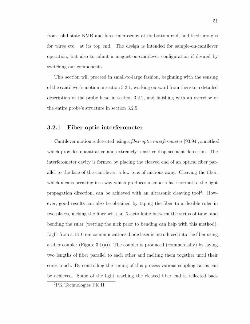
51

from solid state NMR and force microscopy at its bottom end, and feedthroughs

for wires etc. at its top end. The design is intended for sample-on-cantilever

operation, but also to admit a magnet-on-cantilever configuration if desired by

switching out components.

This section will proceed in small-to-large fashion, beginning with the sensing

of the cantilever’s motion in section 3.2.1, working outward from there to a detailed

description of the probe head in section 3.2.2, and finishing with an overview of

the entire probe’s structure in section 3.2.5.

3.2.1 Fiber-optic interferometer

Cantilever motion is detected using a fiber-optic interferometer [93,94], a method

which provides quantitative and extremely sensitive displacement detection. The

interferometer cavity is formed by placing the cleaved end of an optical fiber par-

allel to the face of the cantilever, a few tens of microns away. Cleaving the fiber,

which means breaking in a way which produces a smooth face normal to the light

propagation direction, can be achieved with an ultrasonic cleaving tool2. How-

ever, good results can also be obtained by taping the fiber to a flexible ruler in

two places, nicking the fiber with an X-acto knife between the strips of tape, and

bending the ruler (wetting the nick prior to bending can help with this method).

Light from a 1310 nm communications diode laser is introduced into the fiber using

a fiber coupler (Figure 3.1(a)). The coupler is produced (commercially) by laying

two lengths of fiber parallel to each other and melting them together until their

cores touch. By controlling the timing of this process various coupling ratios can

be achieved. Some of the light reaching the cleaved fiber end is reflected back

2PK Technologies FK II.

52

into the fiber by the cleaved face. Most of the light exits the fiber, and some is

reflected off of the cantilever face and reenters the fiber core, interfering with the

light reflected from the cleave (Figure 3.1(b)). As this light propagates back up the

fiber, the coupler allows it to be directed to a photodiode, the output of which is

amplified. Initially a photodiode was used which was packaged for soldering into a

circuit board—it had a built-in (transresistance) preamplifier, the output of which

was sent to a standard op-amp amplifier circuit low passed at 200 kHz [95], and

an input lens which was epoxied to a standard fiber connector jack (FC-APC) by

hand. Recently this has been replaced with a commercially produced unit which

has an FC-APC fiber input and BNC voltage output, and knobs which control

and filtering frequencies—one of the advantages of working with communications

lasers.

As shown in Figure 3.1(c), the output of a fiber-optic interferometer has a

sinusoidal dependence on the distance d between the fiber face and cantilever,

with wavelength λ/2, where λ is the laser wavelength. The factor of two comes

from the fact that the light traverses the interferometer cavity twice, so a change in

distance δd produces a change in round-trip path length of 2δd. The interferometer

voltage output is well described by

V = V0 +Vpp

2cos

(

4πd

λ

)

, (3.1)

where Vpp is the peak-to-peak voltage amplitude of the interferometer fringes, also

called the fringe depth.

The interferometer uses a “90/10 coupler”, meaning 10% of the light is coupled

from one fiber to the other (from the top fiber to the bottom, or vice-versa, in

Figure 3.1(a)). This means that 90% of the laser light is being thrown away,

however this is not important—the laser can output milliwatts of power, and only

53

signal outcantilever

(b)

d

(d)

V

l/2

coupler

optical fiber

(a)

d

1.5

1.4

1.3

1.2

1.1Inte

rfero

mete

rO

utp

ut

[V]

100806040200

Step

(c)

Figure 3.1: (a) Schematic of the fiber optic interferometer. Thick lines rep-

resent optical fiber. Light from a laser diode is sent to a fiber coupler. Some

of the light is thrown away, and the rest is sent to the cleaved end of an op-

tical fiber which forms an interferometer cavity with the cantilever face. The

interfering light propagates back up the fiber and is collected at a photodiode

on the same side of the coupler and amplified as a voltage signal. (b) The

interferometer cavity formed by the cleaved end of the fiber and the cantilever

face. Light reflected of the inner face of the fiber cleave interferes with light

reflected from the cantilever, producing interference. (c) The output is sinu-

soidal in the distance between the fiber cleave and the cantilever. Sensitive

displacement measurements are made in the approximately linear part of the

curve indicated with a circle. (d) Output of the fiber-optic interferometer as a

function of a stepped displacement.

54

microwatts are needed at the cantilever. More importantly 90% of the valuable

reflected light, which carries the signal, is retained. Furthermore, the coupling

of reflected light back into the laser, which can cause instabilities in the laser

frequency, is minimized. For sensitive measurements of displacements much smaller

than λ/4, the interferometer is tuned to the steep, approximately linear region of

the curve indicated by a circle in Figure 3.1(c). Here, the distance dependence of

the interferometer output, equation 3.1, for a small change in voltage δV , can be

well approximated by

δd ∼= λ

2πVpp

δV. (3.2)

This provides a method of calibrating the interferometer during an experiment by

measuring Vpp, which can be accomplished by exciting the cantilever with a piezo-

electric actuator mounted near its base, by manually striking the probe, or by some

other method, so that its motion is large enough to span at least one interferometer

fringe. This also allows a quantitative analysis of the smallest displacements which

can be measured, by comparing the voltage a given displacement would produce

to the voltage noise at the output. For cantilever motions in the kHz range the

interferometer gives a displacement sensitivity of ∼ 1 pm/√

Hz.

Tuning of the interferometer is achieved by adjusting the temperature, and

thereby the output wavelength, of the laser diode with a thermoelectric cooler [96].

(This is evidently a popular strategy in communications technology as well, be-

cause the laser and thermoelectric cooler come packaged as one unit.) If there are

of order 100 wavelengths in the interferometer cavity (round-trip), only about a

1% wavelength change is required to tune over more than one fringe, and so this

difference did not need to be taken into account when calibrating the interferom-

eter. The TEC only provides about a 1% wavelength change, so the tuning range

55

must be tested when aligning the fiber—if the temperature scan range is less than

one fringe the fiber-cantilever distance is increased. When setting up cryogenic

experiments, a range of about two fringes should be observed at room temperature

since the fiber-cantilever distance can shrink considerably when cooling. The DC

output of the interferometer is sometimes measured continuously during experi-

ments and servoed with a low-frequency PI controller implemented in LabVIEW,

to combat drift due presumably to thermally induced changes in the cavity length.

Often, however, it is found that the interferometer cavity is stable enough that

the laser temperature can be set once at the beginning of the experiment, then

checked every hour or so.

The interferometer can be used for DC displacement measurements, but is less

sensitive for this purpose due to 1/f noise in the interferometer amplifier. Figure

3.1(d) shows a number of interferometer readings taken as the cavity length was

stepped. Here the cavity was not formed with a cantilever but with a reflector

mounted on a coarse approach mechanism, described in section 5.3. The inter-

ferometer allowed the average step size to be measured at 8 nm, within about

10%.

3.2.2 Probe head

The probe is designed for sample-on-cantilever experiments (see section 1.2.1).

The probe head essentially consists of the optical fiber, cantilever, rf coil, and

a number of brass pieces designed to hold them in this configuration. However,

with slight modifications to the cantilever holder and magnetic particle mount,

described below, magnet-on-cantilever experiments could be performed with this

apparatus as well.

56

B

optical fiber

rf coil

magnetic particle

cantilever

Figure 3.2: Schematic of the main experimental components. In the “sample-

on-cantilever” configuration, the sample is glued to the end of the cantilever.

A force is produced between spins in the sample and a magnetic particle fixed

nearby.

57

The optical fiber is epoxied into a stainless steel tube of outer diameter 1/16”,

and inner diameter 0.020”, and about 1.5 cm in length3. Epoxy is only used

at the front end of the tube (the one nearest the cleaved end of the fiber) so

that differential contraction does not strain the fiber when cooling to cryogenic

temperatures. A tight polymer coating placed on the fiber by the manufacturer

is retained to within approximately 1 cm of the cleave, to prevent nicking of the

fiber by the stainless steel tube as it exits at the non-epoxied end4. The stainless

steel tube is placed into a hole in a brass holder, shown in Figure 3.3, and held in

place with a set screw. This piece also carries the cantilever, and will be referred

to as the “cantilever holder”.

The cantilevers used with this probe are commercially produced Si3N4 contact-

mode AFM cantilevers 5, which protrude from a glass die about 1 mm × 2 mm ×

0.5 mm in size. The cantilevers are parallel with the longest dimension of the die

and bend in the direction of its shortest dimension. The fiber and cantilever are

manually aligned as follows. With the cantilever holder held in a vice, a cantilever

die is placed on a drop of 5-minute epoxy and the cantilever’s end is aligned with the

optical fiber before the epoxy sets. Alignment is judged visually by observation

with a long-focal-length stereo microscope while the cantilever die’s position is

adjusted manually, with a toothpick or other small implement. Incoherent white

light can be shone through the fiber to facilitate location of its core. The distance

between the fiber and cantilever is adjusted by loosening the set screw and sliding

the stainless tube in its hole. This is done beforehand using a dummy cantilever

3These are cut from 1-foot lengths available from Small Parts.4This coating prevents the fiber from coming into contact with moisture in the

air. Moisture helps cracks propagate in glass, and will make the fiber extremelybrittle within a few days.

5Veeco model # MSCT-NO, cantilever C.

58

counterbored 0-80clearance hole

0-80 set screw

cantilever die

optical fiber

Figure 3.3: Mount which holds optical fiber aligned with cantilever, called

the “cantilever holder” in the text. The optical fiber is epoxied into a stainless-

steel tube, which is held into the brass cantilever holder with an 0-80 set screw.

The cantilever die is epoxied to the holder. The inset shows, approximately to

scale (the optical fiber is 125 m in diameter), the completed arrangement of

the cantilever and fiber.

59

(i.e. one which might be broken in the process without undue emotional strain

on the experimenter). The inset at the right of Figure 3.3 shows a fiber aligned

to a cantilever protruding from a die, drawn roughly to scale. The 125 micron

cantilever can be used as a scale bar.

Once the cantilever and fiber are epoxied and set screwed, respectively, in this

way, the set-up is extremely robust. If carefully aligned, the fiber will almost

certainly stay aligned down to 4 K, and the epoxy rarely releases upon thermal

cycling.

The position of the cantilever/fiber unit with respect to the rf coil is adjusted

by means of the assembly shown in figure 3.4. The three plates shown in Figure

3.4(a) provide two orthogonal directions of motion. Plate A has three holes near

its circumference through which three 1/16” brass rods pass, providing a third

dimension of motion. The cantilever holder bolts to plate B (Figure 3.4(a)) via

two 0-80 screws. Plate B is then clamped between plates A and C. Plate B is

slightly thicker than plate C so that when the plates are assembled (Figure 3.4(b))

plates A and C do not touch. Plate A has a ledge against which the flat at the

top of plate C rests, and which acts as a guide when sliding plate C. The bolts

which hold the plates together pass through slots in plate C, allowing adjustment

in this direction. Plate B is held down by plate C via its thin edges. Its thicker

center section fits in the wide slot in the center of plate C. When the bolts are

loose plate B can slide in the vertical direction in Figure 3.4. Figure 3.4(b) shows

the assembled positioner. The coaxial cable which carries the rf coil is represented

by the black circle.

A diagram and photograph of the probe head is shown in Figure 3.5. The

positioning assembly discussed in the previous three paragraphs is labelled (ii).

60

(b)

B(a) CA

Figure 3.4: Position adjustment mechanism for the cantilever and optical

fiber. (a) The three plates which make up the positioner. The cantilever

holder (Figure 3.3) is bolted to plate B. Plate C is bolted to plate A with plate

B sandwiched between. (b) The assembled positioner. The position of the rf

coaxial cable is indicated by a black circle.

61

Two of the three rods which hold the assembly together are clearly visible in Figure

3.5(b). (The rods are omitted from Figure 3.5(a) for clarity.) The rf coaxial cable

is clamped against two Macor rods in (i) by a nylon set screw. The nylon set

screw may contract significantly upon cooling to cryogenic temperatures, but the

Macor will not. As long as the contraction of the nylon screw is not so much

that it loses tension, the coaxial cable will be held in position by the Macor rods.

Thus this method provides a method of holding the coax which is adjustable,

electrically insulating, and robust to thermal deformation. Assembly (ii) allows

the cantilever/fiber combination to be located with respect to the coil, as discussed

in the previous paragraph.

The annular plate (iii) bolts to the three brass rods and anchors the magnetic

particle positioner assembly, which comprises also plates (iv) and (v), also annular,

which are not attached to the three rods. Plate (v) is bolted to plate (iii) through

wide clearance holes in plate (iv). Tightening the screws compresses springs be-

tween plates (iv) and (v), holding the magnetic particle mount between plates

(iii) and (iv). The magnetic particle mount is a cylinder which passes through

plates (iii), (iv), and (v), and possesses a circular flange of larger diameter which is

clamped between plates (iii) and (iv). Passing through the center of the magnetic

particle mount is a 2-56 screw, the head of which is visible at the lower right of

Figure 3.5(b). Into the tip of this screw is drilled a small hole into which a glass

capillary of O.D. approximately 0.5 mm is epoxied. The magnetic particle is epox-

ied into the end of this capillary. The capillary and particle are drawn in black in

Figure 3.5(a).

The inset at the lower right of Figure 3.5(b) shows a closeup of the main

experimental components. The cantilever die, labelled “a”, is clearly visible but

62

(ii) (iii) (iv) (v)(i)

b

ac

(ii)

(iii)(iv)

(v)

(i)

(a)

(b)

Figure 3.5: (a) Diagram and (b) photograph of probe head. The overall

structure is circular plates which are clamped to three rods, not shown in (a)

but clearly visible in (b). In the higher magnification inset, lower right, the

cantilever die, rf coil, and the glass capillary which carries the magnetic particle

are visible, labelled a, b and c, respectively.

63

the cantilever itself is not. The cantilever lies at the lower end of the die near

the rf coil, labelled “b”. The glass capillary which carries the magnetic particle is

labelled “c”.

3.2.3 Radiofrequency coil and matching network

The rf coil is approximately 0.8 mm in diameter, and is wound manually using

one lead of a standard 1/4-W resistor as a form. The tip of the resistor lead is

filed round to facilitate removal of the coil after winding. The two leads of the coil

are then trimmed and tinned for soldering. The coil provides an inductance which

is placed in parallel with a capacitor, called the tuning capacitor CT , creating a

resonant LC circuit. This is put in series with another capacitor, the matching

capacitor CM , in order to transform the impedance of the parallel LC to 50 Ω on

resonance. This tuned and matched unit is called the tank circuit. The situation

here is much as in conventional NMR, except the coil inductance is much smaller.

There are two reasons why a small coil is desired. First, the field inside the coil

for a given current increases as the coil is made smaller. On the axis of a circular

loop of wire the field is given by [15]

B =µ0I

2

r2

(r2 + x2)3/2, (3.3)

where r is the radius of the loop, I is the current, and x is the distance from

the plane of the loop. Note that this expression scales approximately as r1/2. By

making the coil small, then, a given field can be obtained with a relatively low

current. This has two advantages. First, the power dissipated in the coil goes as

I2, so the heat deposited in the coil is reduced. In MRFM thermal stability is

important in keeping the small distances between the experimental components

64

constant, especially in cryogenic experiments. Secondly, a low current means low

voltage developed in the coil, which is important because stray electric fields can

excite the cantilever.

The solenoidal formula for the field is not used because, since the sample lies

outside the coil, and is often placed a distance from the coil similar to the interturn

spacing, the first turn of the coil produces the majority of the field at the sample.

The other turns of the coil mostly exist to create a sufficient inductance so that a

resonant circuit can be practically formed. Using equation 3.3 allows an estimate

of the field to be made which takes into account the coil-sample distance. And

because the other turns are not considered in the estimate the experimenter is less

likely to overestimate the field.

Of course, the above assumes that the current in the coil is known, which is not

always the case, especially when using such a small coil—stray inductances and

capacitances can become important, and the coil resistance is not necessarily the

largest one in the circuit. For this reason estimates of the rf field should be made

conservatively.

For a resonant LRC circuit on resonance the resistance can be written in terms

of the quality factor [95],

Rcoil =Lωcoil

Q, (3.4)

where ωcoil is the resonance frequency of the coil. The coil inductance may be

estimated by using the solenoid formula, L = µ0N2A/l, where N is the number of

turns, A is the cross-sectional area of the coil, and l is the length of the coil.

The rf coil consists of 2.5 turns of 36-gauge bare Cu wire. Assuming a radius

of 0.4 mm and a length of 0.8 mm, this gives an inductance of L ≈ 5 nH. Using a

Q of 175 for the tank circuit (as estimated by a reflected-power spectrum) and a

65

l/2 line

CT

CM

L

Figure 3.6: Schematic of half-wave-line radiofrequency tank circuit.

resonant frequency of ωcoil = 2π×350 MHz, equations 3.3 and 3.4 give an estimated

transverse field of 55 G at 1 W in the laboratory frame, i.e. 27.5 G at 1 W in the

rotating frame at a location 0.4 mm away from the coil. (This, as will be seen in

section 3.3.2, turns out to be an overestimate.)

The properties of the coil and the capacitors change with temperature. For

this reason tunable CT and CM are used so that the tank circuit can be reliably

tuned and matched at various temperatures. This presents a design problem:

tunable rf capacitors are generally quite large, and placing them near the coil would

make it extremely difficult to place other necessary items, such as the magnetic

particle positioner, near the sample. The solution devised for this probe is to

separate the coil and capacitors by a half-wave line, as in figure 3.6. A half-

wave, or λ/2, line is a transmission line which is one half wavelength long for the

frequency being transmitted (the wavelength calculation should take into account

the reduced propagation speed of electromagnetic waves in the line). A half-wave

line is in principle indistinguishable from a transmission line of zero length, so with

the coil soldered at one end of the line (across the center pin and outer conductor)

and the capacitors at the other, the tank circuit behaves as if the coil were directly

connected to the capacitors, allowing the inconveniently large, tunable rf capacitors

can be located outside of the main probe head region. The half-wave line is made

66

of Cu to carry heat away from the coil.

The reader may wonder, at which frequency is the line length exactly λ/2,

since the resonant frequency of the tank circuit is tunable? The answer is that

frequencies were chosen such that the half-wave line is slightly too short, with

the effect that the impedance of the coil was rotated slightly counterclockwise.

This was found to have a beneficial effect on the performance of the circuit. The

inductance of the coil is so small that only the very upper end of the tuning

capacitor’s range could be used. With the slightly detuned half-wave line, the coil’s

relatively large resistance is transformed partially into an inductance, allowing

more of the tuning capacitor’s range to be used.

3.2.4 Vacuum system

The vacuum system for this probe is designed for pressures in the 10−6 Torr

range, more than sufficient for preventing reduction of the cantilever quality factor,

which stops improving with decreasing pressure at about 10−3 Torr, and sufficient

for working at cryogenic temperatures.

The vacuum system is based on a 1.5” O.D. stainless steel tube about 1.5 m

long. The bottom end of this tube is silver soldered to Cu ring which forms one

side of a conical grease seal [97], also known as a “1-degree seal”, since the conical

faces of the seal are machined to an angle of approximately 1 degree. The probe

head is also bolted to this ring, providing thermal contact to the outside world.

There are tapped holes in the ring to which Cu braid can be bolted if more cooling

is required at a specific point in the probe. To the other side of the 1-degree

seal attaches a Cu cylinder, 1.5” O.D., 6” long, and capped at the bottom. The

1-degree seal closes the lower end of the vacuum system and allows quick access

67

to the probe head, but with much less width than would be required for a flange.

It can be easily removed by hand when the system is at room pressure, and seals

extremely well when the system is under vacuum (no measurable leak rate with

helium leak detector).

Welded to the top of the stainless tube is a NW-40 flange which is attached to

an NW-40 6-way cross. The remaining five ports of the cross hold feedthroughs

for standard electrical wires, rf, optical fiber, mechanical feedthroughs to control

the rf capacitors, and a valve for evacuation.

Wires are fed into the vacuum space using a hermetically sealed 19-pin military

connector. A commercial o-ring based BNC feedthrough is used for rf signals. The

optical fiber feedthrough is based on a Swagelok connector with its o-ring assembly

replaced with a custom Teflon ferrule [98]. Rods which control the rf capacitors

are passed through Swagelok o-ring seals.

3.2.5 Probe overview

Figure 3.7 shows a schematic overview of the probe. The rods which control

the rf capacitors pass through an NW-40 flange at the top of the probe. Into the

inside of this same flange are welded three 1/4” stainless steel rods, not shown in

Figure 3.7, which forms the “backbone” of the probe structure. Radiation baffles

are soldered to the rods at about 10” spacing. A stainless tube soldered into the

baffles passes the wires and optical fiber down the length of the probe (there are

actually two of these tubes, one for the wires and one for the fiber, but they are

drawn as one in Figure 3.7 for clarity). Stainless steel, semirigid, coaxial rf cable is

passed through another set of aligned holes in the baffles, and electrically isolated

from them by Teflon sleeves. The rf capacitors are mounted to a plate (not shown

68

to rf generator

rf capacitorcontrol rods

to turbopump

to other electronics

half-wave line

rf capacitors

SS vacuum chamber

probe head

Cu vacuum chamber

SS tube

to interferomter

1-degree seal

radiation baffles

Figure 3.7: Overview of the probe in its experimental configuration.

69

in Figure 3.7 for clarity) which attaches to the three stainless rods via holes and

set screws. The stainless rods end near the upper part of the 1-degree seal. Wires,

optical fiber, and the half-wave line pass through the 1-degree seal to the probe

head suspended below.

3.3 Experiment

Electron spin resonance experiments were performed using the probe described

in section 3.2.

The sample was a flake of crystalline diphenyl-picrylhydrazyl (DPPH). DPPH

is an organic molecule with one unpaired electron which makes ESR possible (see

figure 3.8) [35]. It is widely used in the ESR community as a “tune-up” sample.

It readily forms a solid, producing a much higher unpaired electron density than

one usually encounters in solids. All of these qualities make it attractive as a first

sample for any MRFM apparatus.

A flake of DPPH approximately 100 m × 50 m ×10 m was affixed to the end

of a silicon nitride (Si3N4) contact-mode AFM cantilever6. with nominal spring

constant ∼ 10−2 N/m, specified by the manufacturer. The magnetic particle was

a shard of AlNiCo aproximately 0.6 mm long by 0.4 mm wide. Using, as a rough

estimate, a spherical shape with a diameter of 0.5 mm, a tip-sample distance

of 0.3 mm, and a remanance field of 1 T, equation 1.4 gives a field gradient of

∼ 300T/m. Assuming a resonance linewidth of ∼ 20 G (see, e.g. Figure 3.11), this

gives a sensitive slice width of ∼ 7 m, similar to the width of the sample.

An external magnetic field was provided by a resistive electromagnet, formed

by winding two layers of 16-gauge Cu magnet wire around a Cu spool on a lathe.

6Veeco model # MSCT-NO, cantilever C.

70

N

N

NO2

O N2

NO2

Figure 3.8: Molecular structure of DPPH. The dot indicates an unpaired

electron, associated with one of the middle nitrogens, which makes the molecule

paramagnetic.

The spool was machined to fit closely around the probe. The coil consisted of two

layers of windings, at a turn density of 714± 20 turns/m, giving a coil constant of

17.9 ± 0.5 G/A.

After an initial evacuation to ∼ 10−6 Torr, the probe was backfilled with ∼ 100

cc of He gas to exchange heat between the probe and the walls. The end of the

probe, with the magnet mounted on it, was then submerged in liquid nitrogen

(LN2). After the probe cooled to ∼ 80 K, the He gas was pumped back out.

Thermal contact between the probe and Cu vacuum can was somewhat weak,

through the 1/16” brass rods. The probe equilibrated during experiments at ∼

85 K. Since temperature was not critical in these experiments this was deemed

sufficient, and Cu braid was not used.

Working in LN2 reduced the thermal cantilever vibration noise, as well as pro-

viding a convenient way to carry heat away from the magnet. However, at magnet

currents above 8 A the vibrations due to boiling of LN2 excited the cantilever at

71

an unacceptable level. At the maximum practical current of 8 A, the coil was

estimated to produce 143 ± 4 G in its center.

Modulation of the sample magnetization was achieved by the cyclic saturation

method [24,36] (see Figure 3.9). The rf field was turned on and off at a frequency

fmod. When the rf was on the sample magnetization was partially saturated, as

described in section 2.2.5, reducing the magnetization to some value Msat. When

the rf was turned off, the thermal polarization recovered in a time T1, which is

tens of ns for electrons in DPPH [35]. As long as T1 < 1/fmod there should be

some modulation of the sample magnetization. Here fmod was set to the cantilever

resonance frequency fc, a few kHz, so T1 ¿ 1/fmod, and the modulation of the

sample magnetization was nearly square.

The rf was generated by an HP signal generator, the output of which was fed

to a TTL-controlled rf switch (see Figure 3.10). The switch was controlled by the

TTL output generated by the reference of the lock-in amplifier (Stanford SR830).

The lock-in was set to internal reference mode, and the reference frequency was set

to fc, measured just before the experiment. When the rf frequency coincided with

the Larmor frequency of the electrons in part of the sample, the intermittent rf

signal modulated the sample magnetization, producing an oscillating force between

the sample and the magnetic particle. This oscillating force caused a resonant

excitation of the cantilever, which was measured with the fiber-optic interferometer

and demodulated with the lock-in.

For a reference frequency which is exactly equal to fc, the response of the

cantilever should be π/2 out of phase with the drive signal. Therefore the signal

should be concentrated entirely in the quadrature (“Y”) channel of the lock-in

output, with none in the in-phase (“X”) channel.

72

Msat

P

M0

mag

net

izat

ion

rf p

ow

er

time

1/fc

Figure 3.9: Cyclic saturation modulation scheme. (a) The rf field is turned

on and off at a the cantilever resonance frequency. (b) When the rf is on,

the magnetization becomes saturated, and is reduced to Msat. When the rf is

turned off, the thermal magnetization M0 is recovered in a time T1, a process

indicated by the curved edges of the recovering magnetization. The time this

takes is greatly exaggerated in the figure.

73

laser

rfswitch

diode

interferometer

Y

coupler

input

reference

X

square-wavemodulated rf

lock-in amplifier

rf generator

CW rf

Figure 3.10: Block diagram of ESR experiment.

3.3.1 Results

Figure 3.11 shows the lock-in output as a function of external magnetic field.

The interferometer output voltage is converted to a displacement using equation

3.2. Indeed the signal is mostly present in the quadrature phase (circles) of the

cantilever response. The in-phase response (line) shows a slight resonant response,

due to the imperfect match between the lock-in reference frequency and fc, leading

to a cantilever response not exactly π/2 out of phase with the drive. This is

unavoidable due to the finite precision of the lock-in internal reference frequency.

Notice that both channels show a (negative) background response away from

resonance. This is probably due to periodic heating of the cantilever or its support

structure, and is a major drawback of the cyclic saturation technique. The fact

that the response is so similar in the two channels has no significance—the phase

of the background signal was unpredictable, and different on different days. This

background could be avoided by modulating at half the cantilever frequency [24]

74

2.5

2.0

1.5

1.0

0.5

0.0

can

tile

ver

am

pli

tud

e [n

m]

-100 -50 0 50 100

field [G]

Figure 3.11: The in-phase (line) and quadrature (circles) response of the can-

tilever as a function of external magnetic field strength for sample-on-cantilever

ESR of DPPH. The signal is mostly present in the quadrature phase.

75

or employing anharmonic modulation [29], as described in section 1.2.1. However,

for the purposes of these experiments this was not deemed necessary.

Figure 3.12 shows another ESR experiment with similar experimental parame-

ters. Here the distance between the magnetic particle and the sample was increased

compared to the previously discussed experiment, so the resonant field had to be

mostly provided by the electromagnet (notice that the positive-field peak shows

up at a much higher applied field than in Figure 3.11). The field provided by the

magnetic particle was low enough that it could be overcome in the negative field

direction, and a second peak appeared. Notice also how much smaller the signal

is than in Figure 3.11, because with the magnetic particle farther away the field

gradient at the sample is much smaller. Whether a given peak points up or down

depends on whether the interferometer is tuned to a positive or negative slope (see

section 3.2.1). But the two peaks must have opposite sign—one is an interrupted

upward force, the other an interrupted downward force, because the applied field

will determine the direction of the sample magnetization, but is not large enough

to change the direction of the tip magnetization—and therefore opposite phase

with respect to the lock-in reference.

Measuring both peaks allows the tip and applied fields to be disentangled. Let

Bpos be the applied field at which the positive-field peak appears, and Bneg be that

of the negative-field peak. Then

Bpos = B0 −Btip, (3.5)

and

Bneg = −(B0 +Btip). (3.6)

76

0.35

0.30

0.25

canti

lever

am

pli

tude

[nm

]

-100 0 100

field [G]

Figure 3.12: ESR experiment showing resonance peaks at positive and neg-

ative field.

77

Subtracting these equations and rearranging gives

B0 =Bpos −Bneg

2. (3.7)

For the data in Figure 3.12, Bpos = 90 G and Bneg = −140 G, giving B0 = 115

G. Dividing the rf frequency ω0/2π = 350 MHz by this quantity gives a measured

gyromagnetic ratio of γm∼= 3.0 × 1010 Hz/T, which compares fairly well with the

electron gyromagnetic ratio γe = 2.80 × 1010 Hz/T [21]. The largest source of

error is the estimation of the coil constant—indeed, if the coil constant were an

important parameter in these experiments, this measurement could be used to

calibrate it to higher accuracy.

3.3.2 Power broadening

As discussed in section 2.2.5, the saturation signal should get larger and wider

in frequency as the input power is increased. Power broadening can be used as a

method of measuring B1, which is an important figure of merit for one’s rf circuitry,

and especially important here because of the unconventional pairing of a half-wave

line with such a small inductance. Here experiments are described in which the

strength of B1 is extracted from a power broadening measurement.

In DPPH, T1 ≈ T2, [35] so equation 2.36 is appropriate. Recasting 2.36 in field

units by dividing by γ2eT

21 gives

Mz(B) = M01/γ2

eT21 + (B −B0)

2

1/γ2eT

21 +B2

1 + (B −B0)2. (3.8)

In DPPH at 77K, 1/γ2eT

21 ≈ (1.3 G)2 [99]. Figure 3.13 shows a number of curves

collected at various rf powers, along with fits of the data to equation 3.8 with

1/γ2eT

21 = (1.3 G)2. As expected, as the input power is increased the curve becomes

78

-1.4

-1.2

-1.0

-0.8

-0.6

-0.4

-0.2

0.0

0.2

dis

pla

cem

ent

[nm

]

1201101009080

field [G]

Figure 3.13: ESR resonance spectra at various rf powers (solid lines) with

fits to equation 3.8. From the top, the powers are 126 mW, 158 mW, 200 mW,

251 mW, 316 mW, 398 mW, 501 mW, 631 mW, 794 mW, 1000 mW, 1259 mW

and 1585 mW.

“deeper” and wider. Also, the background driving of the cantilever increases with

the input power.

But is the value of B1 given by fitting equation 3.8 to these data accurate?

The above analysis fails to take into account the fact that signal is collected from

electrons throughout the sensitive slice, which experience a range of fields, and

that the sample has finite thickness. The simplest way to account for this is to

add a constant to the denominator of equation 3.8—this will have the effect of

broadening the steady-state magnetization curve by an amount which does not

depend on the input power. Because B1 is proportional to the current in the coil,

and the power P dissipated in the coil is proportional to the current squared, one

79

50

40

30

20

B1ef

f22

[G ]

1200800400

power [mW]

Figure 3.14: Power dependence of width of ESR resonance curves.

expects that B21 ∝ P . So in this simple model of the tip-broadened saturation

spectrum, define the effective transverse field as

B1eff(P ) ≡ B21(P ) + β = αP + β. (3.9)

Figure 3.14 shows the values of B21eff obtained from the fits in Figure 3.13,

plotted as a function of rf input power. A line fit to the data indicates that

the coil is producing 5 G/√

W in the rotating frame. This result is somewhat

disappointing—a transverse field of greater than 20 G is required for most pulsed

solid-state NMR experiments, which would require 16 W rf pulses. This would

likely place an unacceptable heat load 4 K MRFM experiments. Had the circuit

performed as estimated in section 3.2.3 it would only have required 1 W.

A likely cause is the presence of the half-wave line, which places a resistance

in series with the coil. Also, there could be stray capacitances and inductances in

80

the relatively large circuit elements at the tuning-capacitor end of the tank circuit

which are not accounted for in a lumped-element analysis. These could alter the

coupling to the half-wave line, making the current at the coil unpredictable. It

should be said that the model used here in the power broadening measurement

is somewhat crude—however this measurement was confirmed by a much more

reliable method, described in Chapter 4.

3.4 Conclusions

In summary, a sample-on-cantilever MRFM apparatus was described which cen-

tered on a half-wave-line-based rf tank circuit. The probe is designed for variable-

temperature, sample-on-cantilever MRFM experiments and for testing in a transfer

dewar. Cantilever motion is detected with a fiber-optic interferometer, and a trans-

verse rf field is provided by a half-wave-line-based tank circuit with a ∼ 0.8 mm

diameter coil. MRFM experiments were performed detecting ESR in DPPH in the

sample-on-cantilever configuration. A gyromagnetic ratio measurement provided

strong evidence that electrons were responsible for the observed signal. Power

broadening experiments were performed, indicating a B1 field of 5 G/√

W in the

rotating frame, far short of the estimated value of 27.5 G/√

W. This unexpect-

edly low figure is confirmed by nuclear nutation measurements in Chapter 4, and

is attributable to the added resistance of the half-wave line or possibly unknown

phase shifts in the tank circuit.

CHAPTER 4

FORCE-DETECTION OF NUCLEAR MAGNETIC RESONANCE

IN AMMONIUM NITRATE

4.1 Introduction

This chapter describes room-temperature MRFM experiments in which 1H

NMR is detected in ammonium nitrate. Experiments are performed in high vacuum

with a commercial, contact-mode AFM cantilever, just as in Chapter 3, which gives

a force sensitivity of 5 fN/√

Hz. This sensitivity is relatively low by modern MRFM

standards, but that does not reduce the significance of these measurements—the

manipulation of nuclear spins provides vital information on the quality of the B1

field.

The experiments described in this chapter use the cyclic ARP modulation tech-

nique, in which the spins must stay locked to the rf field during the entire signal

collection period. Because MRFM uses much longer spin-lock times than in con-

ventional NMR (often > 1 s), this makes exceptional demands on the quality of

the rf. Yannoni has performed experiments spin-locking nuclei with long T1ρ values

using a variety of rf sources, and found that the lock times depend strongly on the

phase noise of the source [100]. Shorter lock times mean a larger measurement

bandwidth, and therefore reduced SNR. For this reason it is extremely important

to have low-phase-noise rf in nuclear MRFM experiments, and to test whether

digitally synthesized rf waveforms—desirable for the complicated pulse sequences

necessary for the Fourier-encoded imaging protocol of Kempf and Marohn [18], or

for advanced ARP modulation schemes [20]—could achieve this high standard.

In section 4.2 the rf generation apparatus used to create the signals for ARP-

81

82

based MRFM is described. Section 4.3 presents the results of initial 1H NMR

MRFM experiments in ammonium nitrate. In section 4.4 experiments will be de-

scribed in which fully digitally-synthesized, pulsed MRFM is demonstrated, pro-

viding a pulsed-NMR measurement of B1.

4.2 Experiment

Experiments were performed in the sample-on-cantilever configuration1. The

sample was ammonium nitrate, chosen for its relaxation properties, i.e. T1 ≈

T1ρ ≈ 1 s at room temperature [26]. For this reason it makes a very attrac-

tive MRFM sample for room-temperature experiments. However, care must be

taken that too much time is not left between evacuating the probe and performing

measurements—ammonium nitrate sublimes in vacuum! A flake of ammonium ni-

trate, approximately 100 m × 50 m × 10 m, was glued to the end of a cantilever

with 5-minute epoxy, as in the previous chapter.

The external polarizing field B0 ≈ 8 T was provided by a liquid-He cooled

superconducting magnet. The dewar was equipped with a vacuum-insulated insert2

which provided a space of 3” diameter in the magnet center and isolated from the

liquid He, and which admitted He gas from a heated nozzle through a capillary

from the liquid He reservoir. During experiments He gas heated to approximately

300-325 K was flowing through this sample space. At these gas temperatures the

probe was found to equilibrate at a temperature of ∼ 290 K.

The sample magnetization was modulated at the cantilever mechanical reso-

nance frequency by the cyclic ARP technique [26], in which repeated ARP sweeps

1The apparatus used here may be assumed to be the same as that described indetail in chapter 3 except where differences are mentioned.

2Custom Janis SuperVariTemp system.

83

(see section 2.2.7) adiabatically tip the magnetization from up to down and back

again. A Schematic of the modulation scheme is shown in figure 4.1. A triangular

frequency modulation was employed. (Sinusoidal [26] and tangential [20] mod-

ulation have been demonstrated by other researchers.) The adiabatic condition

(equation 2.38) puts a limit on the modulation width Ω because a full sweep must

be completed during half a cantilever cycle. Recasting equation 2.38 in these terms

gives

Ω ¿ γ2B21

4f0

, (4.1)

where f0 is the cantilever frequency.

The rf was generated in one of two ways, to be referred to here as “analog”

and “digital”. In the analog method, shown in Figure 4.2(a), a computer and

a digital-to-analog converter (DAC) were used to produce synchronized control

voltages. A voltage proportional to the desired modulation waveform, consisting

of an initial large sweep, then many triangular cycles at the cantilever frequency,

a few kHz, and finally another large sweep away from resonance, as in Figure

4.1(a), was sent to the FM input of the rf generator. The rf generator’s center

frequency was set to the tank circuit resonance, ∼ 350 MHz. A TTL pulse train

at the cantilever frequency was sent to the lock-in amplifier’s (Stanford SR830)

reference input. This signal was synchronized with the lock-in reference signal so

that phase-coherent lock-in detection could be used. The TTL signal began before

the FM voltage by an amount of time sufficient for the lock-in to lock to the signal,

∼ 75 ms. A TTL pulse was used to turn on and off the rf amplifier, as in 4.1(b)3.

In this method the DAC need only create signals in the audio frequency range.

3This pulse was actually supplied by one of the DC voltage outputs of thelock-in amplifier, but is drawn as the same DAC in 4.2(a) for simplicity.

84

Ww

0

M0

mag

net

izat

ion

rf f

requen

cyrf

am

pli

tude

0

-M0

0

time

1/f0

(b)

(c)

(a)

Figure 4.1: A plot of the (a) rf frequency, (b) rf amplitude, and (c) sample

magnetization in the cyclic ARP modulation scheme. Initially the rf frequency

is far from resonance, and at this time, when the spins are least affected by

its presence, the amplifier is turned on. The rf is then swept through the

spins’ resonance frequency ω0 repeatedly, with a modulation amplitude Ω,

and at a frequency which coincides with the cantilever mechanical resonance

frequency. The magnetization remains locked to the effective field, and is

repeatedly inverted in synchrony with the rf frequency modulation. The rf

frequency is brought far off resonance again before the rf amplifier is turned

off.

85

computer

DAC

Y

from fiberinterferometer

on/off

Xlock-in amplifier

rf amplifier

FM

reference

outinput

rf generator

to tankcircuit

computer

high-frequencyDAC

Q

sample clock

rf generator 1

I

(b)

(a)

rf generator 2

rf amplifier

to tankcircuit

Figure 4.2: Block diagram of the frequency modulated rf generation appara-

tus.

Also, since the rf is generated directly by a high-quality rf source the phase noise

of the resulting signal is known. Sources used were the HP (now Agilent) 8657A,

nominal single-side-band phase noise -120 dBc/Hz at 20 kHz off of carrier, and the

HP 8642A, with nominal single-side-band phase noise -137 dBc/Hz at 20 kHz off

of carrier. These values were previously shown by Yannoni to be sufficient for > 1

s spin-lock times [100].

In the “digital” method, Figure 4.2(b), in-phase and quadrature rf signals,

with frequency profile as in 4.1(a), were synthesized using a high-frequency DAC

at ∼ 4 MHz (the intermediate frequency, or IF), then shifted up to the tank circuit

86

resonance frequency, ∼ 350 MHz, using single-sideband mixing [95]. Because the

phase noise of the internal clock in the DAC was not specified by the manufacturer4,

an external sampling clock is supplied by one of the HP sources named in the

previous paragraph at ∼ 100 MHz. The use of an external sampling clock means

that the entire internal timing circuitry of the DAC, which would normally create

the signal at the specified sampling frequency, is bypassed. Instead samples are

released at the zero crossings of the external signal.

In the “digital” method the rf amplifier was left on at all times. The DAC,

in its resting state, i.e. when not producing rf, produced DC signals on both

channels, which led to some degree of carrier bleed-through at the mixer. This was

not problematic as the carrier was displaced from the Larmor frequency by the IF,

∼ 4 MHz, and so did not perturb the sample spins. The effect of this unwanted rf

was further reduced by crossed diodes at the amplifier output. Also, because the

high-frequency DAC had only two outputs, no reference signal for the lock-in could

be provided with this hardware. Thus the lock-in amplifier could not be used in a

phase-coherent manner, and only provided amplitude information.

The cantilever resonance frequency and quality factor were determined by

Fourier transforming either the thermal noise signal (as in Figure 2.7), or a decay-

ing excitation produced by striking the probe manually.

4.3 Results I: 1H NMR

Figure 4.3 shows the output of the lock-in amplifier at two different external

field strengths. Here the “analog” rf generation scheme as in Figure 4.2(a) was

4And therefore almost certainly too high for our purposes, considering the ex-pense and care required to achieve low values.

87

used, at 28 dBm (= 631 mW), with an ARP center frequency equal to the center

of the tank circuit resonance at 352.3 MHz and an ARP width of Ω = 100 kHz.

The cantilever had resonance frequency f0 = 1180 Hz, quality factor Q = 897, and

the probe temperature was measured to be ∼ 300 K. These parameters, along with

the manufacturer-quoted spring constant of 10−2 N/m give a minimum detectable

force of Fmin = 5 fN/√

Hz. The rf excitation began at time 1.8 s and lasted until

time 3.8 s. At 8.240 T, shown as a dashed line, there is no discernible excitation

associated with the rf excitation. The equipartition theorem prediction (equation

2.56) for the rms thermal cantilever noise is ∼ 6.4 A, which compares well to the

observed background noise. At 8.254 T, shown as triangles connected by a solid

line, a cantilever excitation is observed. The fact that it is coherent with the

frequency modulation signal, yet field dependent, already provides strong evidence

that the signal is due to NMR.

After the rf is turned on, the oscillation strength increases according to the

characteristic time of the cantilever. This same effect is observed in the decay of

the excitation after the rf is turned off. The decay in between is consistent with

a magnetization decay. Here the decay time of the signal is on the order of 1 s,

and so the origin of this decay is presumed to be primarily due to rotating-frame

spin-lattice (T1ρ) relaxation.

Figure 4.4 shows a curve formed by taking the lock-in output at time t = 2.5 s,

where the maximum cantilever excitation occurs, from a number of data sets like

the one in Figure 4.3. This gives a result more like a traditional magnetic resonance

spectrum. The peak signal of 53 fN occurs at 8.254 T. The peak is considerably

wider than a conventional NMR resonance peak, due to the field inhomogeneity

due to the tip, the width of the ARP modulation, and the thickness of the sample.

88

4

3

2

1

0

-1

lock

-in

outp

ut [

nm]

6543210

time [s]

6.4 Å

Figure 4.3: Lock-in output during cyclic ARP of ammonium nitrate sample,

at two external field values. The cyclic ARP excitation begins at time 1.8 s and

lasts until time 3.8 s. At 8.240 T (dashed line), a non-resonant field, there is

no discernible excitation associated with the rf excitation. The equipartition

theorem prediction for the thermal noise is ∼ 6.4 A. At 8.254 T (triangles

and solid line), a cantilever excitation is observed, coherent with the frequency

modulation signal.

89

The SNR is about 10, in agreement with the predicted minimum detectable force

of 5 fN.

In fact, the spectrum in Figure 4.4 can be viewed as a one-dimensional image

of the sample—as the external field is changed, the sensitive slice moves through

the sample, giving a signal proportional to the total magnetization in the slice at

each field. The sample was observed with an optical microscope to be flat on the

side glued to the cantilever, and somewhat convex on the other, as in figure 1.1.

Because of the arrangement of the tip, field and sample, which are just as in figure

1.1, the flat side of the sample is farthest from the tip, and therefore comes into

resonance at the highest external field. This is reflected in Figure 4.4—the high-

field side of the peak is much steeper than the low-field side. Using an estimate

for the field gradient based on a spherical particle 0.5 mm in diameter, a 1 T

saturation field for the AlNiCo, and a tip-sample distance of 0.2 mm gives a field

gradient of about 800 T/m. With the peak-to-peak ARP width of 200 kHz used

here, the sensitive slice was approximately 6 m thick.

In order to further confirm that the signal was due to NMR, the tank circuit

was tuned 300 kHz lower in frequency, to 352.0 MHz, and a curve similar to the one

in Figure 4.4 was taken. The result is shown in Figure 4.5. The dashed curve is the

same data as in Figure 4.4. The solid curve shows the response at the new ARP

center frequency of 352.0 MHz. The response has shifted down field, as expected.

To the resolution of the measurement, the shift is from 8.254 T to 8.247 T, a shift

of 70 G. Dividing by the shift in field, 300 kHz, gives an estimated gyromagnetic

ratio of γ ∼= 43 MHz/T, consistent with the proton gyromagnetic ratio of γp = 42.6

MHz/T [21]. This gives a strong indication that the signal is due to 1H NMR.

90

4

3

2

1

0

lock

-in

ou

tpu

t [n

m]

8.288.268.248.22

field [T]

Figure 4.4: Force-detected NMR spectrum from ammonium nitrate, obtained

by plotting the lock-in output at t = 2.5 s from a number of data sets like that

in Figure 4.3.

91

4

3

2

1

0

lock

-in

ou

tpu

t [n

m]

8.288.268.248.22

field [T]

352.3 MHz

352.0 MHz

Figure 4.5: Two spectra collected with different ARP center frequencies. The

peak shifts by about 70 G for a frequency shift of 300 kHz, consistent with the

proton gyromagnetic ratio.

4.4 Results II: pulsed NMR

In this section MRFM nutation experiments are described. As discussed in

section 2.2.6, when an on-resonance transverse (B1) field is applied to a thermally

polarized spin ensemble, the magnetization will precess around the effective field

in the rotating frame, a process called nutation. Nutation can be used as a sensi-

tive measure of B1 strength, because the nutation frequency, also called the Rabi

frequency, is given by ωR = γB1. Nutation was first demonstrated with MRFM in

fluorine nuclei in CaF2 [44], and later in electrons [37].

Nutation experiments were performed in the following manner. First the field

value of maximal signal was located using the methods described in the previous

section. The field was set to this value, and the rf generation apparatus was set up

92

ARP

t t1

rf a

mp

litu

de

time

Figure 4.6: The rf sequence used in nutation measurements. A pulse of du-

ration τ is applied to tip the magnetization away from vertical, after which the

rf is left off for a time t1 in which the in-plane component of the magnetization

decays away. The resulting magnetization projection on z is then read out

with an ARP sequence.

as in Figure 4.2(b). Then an rf sequence as shown in Figure 4.6 was applied. First

a pulse of duration τ was applied at the ARP center frequency. Then the rf was

turned off for a duration t1. The time t1 should be > T2 so that any transverse

magnetization decays away. The resulting magnetization Mp lies along the z axis,

with length equal to the projection of M0 along z after the tipping pulse. Then

an ARP sequence exactly as in the previous section, but generated in the method

of Figure 4.2(b), was applied to measure Mp. The cantilever excitation was not

measured coherently, so the two components of the lock-in signal were Fourier

transformed and integrated, to obtain a signal proportional to the mean squared

cantilever amplitude (through Parseval’s theorem) and therefore proportional to

M2p . After waiting a time À T1, so that the magnetization fully recovered its

thermal polarization, the sequence was repeated with a different pulse duration τ .

The expected behavior of the magnetization projection onto z, Mp, as a func-

93

tion of pulse time τ is shown in Figure 4.7(a). At zero pulse time the magnetization

will be equal to the thermal equilibrium value M0. As the magnetization precesses,

its projection onto z will have a cosinusoidal behavior, with an exponentially de-

creasing envelope with some decay time τm. The squared cantilever amplitude after

a pulse of duration τ should be proportional to M 2p , so will trace out a decaying

squared cosinusoid as τ is stepped, as in Figure 4.7(b).

Figure 4.8 shows the results of the measurement (circles), along with a fit to a

decaying squared consinusoid, plus a constant to account for background cantilever

excitation (blue line). The data show the expected behavior, and the fit provides

a Rabi frequency of ωR = 1.25 × 105 rad/s, which gives B1 = ωR/γp = 4.6 G, in

agreement with the measurement of B1 = 5 G from power broadening in chapter

3.

The fit indicates a decay time of 0.125 s. This decay is likely due partially

to spin-spin relaxation (T2 processes), which sets the decay time in inductively

detected nutation experiments. Here, though, dephasing due to the inhomogeneous

field from the tip probably also plays a significant role. Spins for which the pulse

is nonresonant precess around an effective field which is not perpendicular to z,

resulting in increased dephasing of the spins in different parts of the slice.

4.5 Conclusions

In this chapter experiments were described in which MRFM was used to de-

tect 1H NMR in ammonium nitrate. Force measurements were performed with a

commercially produced AFM cantilever at room temperature in high vacuum, and

were thermally limited with a minimum detectable force of Fmin = 5 fN/√

Hz. A

peak force of 53 fN was detected from a flake of ammonium nitrate with dimensions

94

Mp

tm

A2

M0

tm

(b)

(a)

pulse time t

pulse time t

Figure 4.7: Expected behavior under nutation. (a) The z projection of the

magnetization as a function of pulse time τ . The magnetization is initially at

its thermal equilibrium value M0, and makes a cosinusoidal projection on z as

it precesses. (b) The squared cantilever excitation as a function of pulse time

τ will therefore take the form of a squared cosinusoid.

95

4.0

3.5

3.0

2.5

2.0

1.5

1.0

squ

ared

can

tile

ver

ex

cita

tio

n [

arb

]

30252015105

pulse time [µs]

Figure 4.8: Observed nutation signal (circles) fit to a decaying squared cosi-

nusoid (blue line.)

on the tens-of-microns scale. Observation of a shift in peak location upon changing

the rf modulation center frequency was consistent with the proton gyromagnetic

ratio, which strongly indicates that the signal was due to 1H NMR. Pulsed NMR

MRFM was demonstrated with a digital rf generation scheme. The Rabi frequency

for was measured to be ωR = 1.25 × 105 rad/s, which gives B1 = ωR/γp = 4.6 G

at 1 W of rf power, in agreement with the power-broadening estimate of B1 given

in Chapter 3.

These measurements, by showing that nuclear spins could be spin-locked for

times on the order of 1 s, demonstrate that the rf generation schemes described

here have sufficiently low phase noise for use in nuclear MRFM experiments. The

fact that this is true even for digitally synthesized rf is significant because it allows

more general rf pulse and modulation schemes to be implemented. This is partic-

ularly important for the complicated pulse sequences which must be synchronized

96

with cantilever motions in order to achieve FT-MRFM imaging [18], or for more

advanced frequency modulation schemes such as phase-cycled, tangent-modulated

ARP [20]. However, these experiments also confirm the diagnosis of anemic B1

made in Chapter 3. This and other considerations caused the half-wave line tank

circuit to be abandoned for the high-sensitivity, 4 K experiments described in

Chapter 5.

CHAPTER 5

FORCE-GRADIENT DETECTION OF NUCLEAR MAGNETIC

RESONANCE IN GALLIUM ARSENIDE

5.1 Introduction

In this chapter a unique type of MRFM is described, in which a force gradient,

rather than a force, perturbs a cantilever’s motion. A force gradient has units of

N/m, the same as a spring constant. This suggestive fact leads to a method—

the force gradient acts as an additional (positive or negative) restoring force on

the cantilever, registered as a shift in the cantilever’s resonance frequency. This

property is widely used in AFM experiments [101], but before the experiments

described here had never been applied to MRFM. (This should not be confused

with the OSCAR method, which produces a cantilever frequency shift, but relies

on forces, not force gradients, to do so. This distinction will be made more clear

in section 5.2.2.)

In 2002, when the technique was conceived, MRFM was facing two problems.

The first, as discussed in section 1.2.2, is that ultrasoft cantilevers must be used

perpendicular to the sample surface, but at this time the sensitivity to detect

statistical polarization in nuclear MRFM had not yet been reached. As will be

seen in section 5.2, force-gradient MRFM does not require statistical imbalances

in the spin polarization. Second, all previous nuclear MRFM experiments (and

those at the highest sensitivities achieved with electrons) had required that the

sample magnetization remain spin-locked [85] to an applied radio-frequency field

during the entire signal acquisition period, with the result that signal could only be

collected for a time t ∼ T1ρ, the spin lattice relaxation time in the rotating frame.

97

98

This was the situation, for example, in the experiments described in Chapter 4.

With force-gradient MRFM, signal can be collected for a time approaching T1,

the spin-lattice relaxation time in the laboratory frame. Since often T1 À T1ρ at

cryogenic temperatures, a much wider range of samples should be accessible to

MRFM using the approach introduced here. Also, for samples with T1 ≥ 10 ms,

the method opens up the exciting possibility of following magnetization recovery in

real time in a single-shot experiment. For this reason the technique will be referred

to as CERMIT, or cantilever enabled readout of magnetic inversion transients.

In section 5.2, the CERMIT method will be described in detail and compared

to the other perpendicular MRFM method, OSCAR. An estimate of the signal size

is made for both techniques, and these are put into perspective by comparing to

that given for parallel-cantilever force detection in Chapter 1. In section 5.3 the

apparatus built to demonstrate the technique is described. Results from MRFM

magnet-on-cantilever experiments, using an ultrasoft cantilever, at 4.4 K and 7 T,

are given in section 5.5. Finally, numerical calculations are presented and compared

with observation in section 5.6.

Due to the use of a low-spring-constant cantilever at a relatively low temper-

ature, the measurements described in this chapter achieved world-record nuclear

MRFM sensitivity at the time of their publication [48], representing an improve-

ment of more than 500 times the previous best [44] 1.

1A somewhat higher sensitivity for nuclei was recently reported at the time ofthis writing [102]. Also, the recent detection of a single electron by MRFM had amagnetic moment sensitivity about 50 times higher [40].

99

5.2 Theoretical background

5.2.1 Force-gradient MRFM

As discussed in section 1.2.2, a uniformly magnetized planar sample will pro-

duce no force on a perpendicular cantilever. Figure 5.1(a) shows a perpendicular

cantilever’s tip near a planar sample. The external magnetic field here is assumed

to be along z, and the cantilever is vibrating in the x direction. The force from

spins on one side of the cantilever will be offset by other spins on the opposite side,

and will sum to zero. This is the basic problem which inspired the invention of the

CERMIT protocol.

Now consider the force gradient on the tip. Magnetic moments µ (assumed,

for now, to all be pointing in the +z direction) in the sample interact with the tip

magnet to produce a net force gradient given by

∂Fx

∂x=∑

j

µ(rj)∂2Bz(rj)

∂x2, (5.1)

where Bz is the z component of the field due to the tip, rj is a vector pointing to

the spin, x is the direction of cantilever deflection, and the sum is over all spins in

the sample. This spin force gradient is also zero for a homogeneously magnetized

planar sample [103]. In the CERMIT method, a detectable change in force gradient

is produced by inverting spins in a region under the tip using ARP [Figure 5.1(b)].

Although this inverted region of spins, because of its symmetry, will produce no

net force on the cantilever (in its bending direction), the force gradient it produces

is measurable. The region of inverted spins lies between two constant-Bz contours

determined by the initial and final frequencies of the ARP sweep.

After the sweep the resulting shift in the force gradient, and therefore in the

spring constant, will be equal to the difference between the force gradient before

100

cantilever

tip

cantilever displacement

(a) (b)z

invertedspins

sample

cantilever displacement

pote

nti

alen

ergy

pote

nti

alen

ergy

x

Figure 5.1: The CERMIT experiment. (a) A magnet-tipped cantilever is

placed perpendicular to the sample surface. The forces from spins on the two

sides of the tip cancel to zero by symmetry. The cantilever vibrates according

to its harmonic potential energy function. (b) After an ARP sweep, there is

a slice of inverted spins near the tip. The inverted spins attract the tip, so

there is an energy cost associated with displacing the tip to either side. The

result is that the potential energy function steepens, which raises the effective

spring constant of the cantilever. This change is registered as a shift in the

cantilever’s resonance frequency.

101

and after the sweep:

∆k ≡ ∂Fx

∂x

∣

∣

∣

∣

after

− ∂Fx

∂x

∣

∣

∣

∣

before

= −2∑

j∈slice

µ(rj)∂2Bz(rj)

∂x2, (5.2)

where now the sum is over spins in the slice only. Spins inside the slice contribute

with the same sign in both terms, leading to the factor of two in front of the sum,

whereas spins outside the slice cancel in the difference.

This change in the spring constant shifts the cantilever’s resonance frequency

by an amount ∆f . Since f = (1/2π)(k/m)1/2, for small spring constant shifts this

is given by

∆f ≈ f0

2k∆k (5.3)

This is the quantity which is measured in the experiment.

At each end of the sweep, where the rf is turned on or off, the spins will not

be able to adiabatically follow the effective field, and a “dead” region of decreased

magnetization will be produced. The dead regions will be slices of thickness ∼ Gδ,

where G is the field gradient at the location of the slice and δ is the linewidth of

the NMR resonance of the nucleus under study. These dead regions are expected

to be of negligible width in the experiments described in this chapter. It should

also be mentioned that because the tip is vibrated, the total field at the location

of spins in the sample will be changing during the sweep Tip’s motion must be

kept sufficiently small that the adiabatic condition (equation 2.38) is met during

the sweep.

5.2.2 Estimate of signal size and comparison with OSCAR

This section gives an estimate of the CERMIT signal size, and a compari-

son with that of the OSCAR technique employed by researchers at IBM in high-

102

sensitivity MRFM experiments [38–40]. These will be compared with the expected

force from the parallel-cantilever experiment described in Chapter 1. In order to

effectively compare these techniques, which all measure different quantities, the es-

timates will be cast it terms of SNR for a thermally-limited experiment. Single-spin

detection will be considered in all cases—the different magnetization modulation

schemes involved produce different volumes of active spins, and by considering a

single spin this complication can be removed. The experimenter can always mul-

tiply by the number of spins for the expected sensitive slice to get a practical

estimate (for a good estimate the fact that the gradients won’t be the same over

the whole slice should be taken into account).

The assumption will be made throughout of a spherical magnet of radius a and

magnetization M , with magnetic moment lying along z (see Figure 5.2). In what

follows, the objective is to calculate the interaction of such a magnet with a single

spin magnetic moment, also polarized along z.

Standard force detection

The “parallel-geometry” experiment, with a spin directly below the tip was

considered in section 1.1.1, with the force given by equation 1.5. The SNR for this

experiment is found by simply dividing by the minimum detectable force (equation

2.63), which gives

SNRForce ≈ 0.633µµ0M

aFmin

. (5.4)

This expression provides a convenient reference for the more modern experiments

considered below.

103

CERMIT

For the CERMIT experiment a similar procedure is followed: consider a single

spin directly below the tip and calculate the signal, then maximize with a fixed d.

Here the signal is given by ∆kx = µ∂2Bz/∂z2 where the field gradient is evaluated

at the location of the spin. This gives2

∆kx =4µµ0M

a2

(

a

a+ d

)5

, (5.5)

which for a fixed d has a maximum at a = 3d/2. Putting this into the above gives

∆kx ≈ 0.311µµ0M

a2. (5.6)

To achieve an expression similar to equation 5.4 the above should be divided by the

minimum detectable spring constant shift, defined as the spring constant change

which can be detected with a SNR of one. This is given, for a cantilever oscillating

with amplitude xrms, by [104,105]

∆kmin =Fmin

xrms

, (5.7)

which has units of N/(m√

Hz), as expected3. So the SNR for the single-spin

CERMIT experiment is given by:

SNRCERMIT = 0.311µµ0Mxrms

a2Fmin

. (5.8)

2A minus sign has been omitted for simplicity.3This expression can be understood as follows. A cantilever oscillating with a

rms amplitude xrms in the presence of a force gradient ∂F/∂x experiences a spanof forces throughout its motion of approximately (∂F/∂x)xrms. For the cantileverto “notice” this difference, this quantity needs to be ≥ Fmin. Therefore ∆kmin ≡(∂F/∂x)min = Fmin/xrms.

104

a

x

(b)

a

d

OSCAR

tip

sensitive slice

(a)

d

sample

CERMIT

zx

Figure 5.2: The distances used in the text to describe the CERMIT and

OSCAR experiments. (a) In the CERMIT experiment the tip interacts with

a spin directly below the tip, a distance d from the tip’s surface. (b) In the

OSCAR experiment the situation is the same, except the spin is also displaced

laterally by a distance x.

OSCAR

The OSCAR (oscillating cantilever-driven adiabatic reversals) protocol [38–40]

works, briefly, as follows. The cantilever is oscillated, producing a changing mag-

netic field at the location of the spin. The spin will therefore have a Larmor

frequency which depends on the cantilever position. For clarity in what follows,

define the Larmor frequency for the spin ω0 as its resonance frequency when the

cantilever is at its equilibrium position. At one of the extremes of the cantilever’s

motion an rf field is turned on, at ω0. Because the cantilever is displaced, shifting

the field, this is not experienced by the spin as a resonant field, and if the tip field

gradient (∂Bz/∂x in the coordinates of Figure 5.2) times the cantilever displace-

ment is large compared to the resonance linewidth, ω0 can be said to be far off

resonance at this time. As the cantilever sweeps through its equilibrium position,

105

the field sweeps through resonance, causing an ARP of the spin (assuming the

adiabatic condition is met). Although the roles of the field and rf frequency are

switched here, it operates exactly as ARP as discussed in section 2.2.7 (and indeed

sweeping the field, not the frequency, was the method used in early NMR [65]).

As the cantilever oscillates, the spin is repeatedly inverted in phase with the can-

tilever’s motion. This produces a time-dependent force on the cantilever which,

because it is exactly in phase (or exactly π out of phase) with the cantilever is

indistinguishable from a static force which varies as the position of the cantilever,

i.e. a force gradient, and a shift in the cantilever frequency is observed.

Note that in the OSCAR protocol if the cantilever is perpendicular to the

surface a single spin must be displaced to either side to produce a signal. For this

reason another variable is introduced to the analysis below, namely the transverse

displacement of the spin x, as shown in Figure 5.2(b).

In [39] an estimate of the OSCAR signal size is given which translates to, in

the present notation,

∆f = ± 2µf0

πkxpk

∂Bx

∂z, (5.9)

where xpk is peak-to-peak driven motion of the cantilever. The sign is given by the

phase of the spin flips with respect to the cantilever motion. This can be written

in terms of a spring constant shift via equation 5.3. Choosing the positive sign,

this gives

∆k =4µ

πxpk

∂Bz

∂x. (5.10)

To maximize this expression the tip field gradient is considered as a function

of tip size a, distance from the surface to the magnet center z, and a lateral

106

displacement x. From equation (1.2),

Bz =µ0Ma3

r3

(

3z2

r2− 1

)

= µ0Ma3

(

3z2

(x2 + z2)52

− 1

(x2 + z2)32

)

. (5.11)

Taking the derivative of the tip field is in the x direction,

∂Bz

∂x= µ0Ma3

(

3x

(x2 + z2)52

− 15z2x

(x2 + z2)72

)

. (5.12)

With d fixed (recall z = a + d), a numerical maximization gives x/d ≈ 2.320,

a/d ≈ 3.000, at a value of

∂Bz

∂x≈ −0.096µ0M

(

1

a

)

, (5.13)

so

∆k ≈ 0.384µµ0M

πaxpk

, (5.14)

and

SNROSCAR ≈ 0.043µµ0M

aFmin

. (5.15)

Notice the lack of dependence on oscillation amplitude—the xpk from equation

5.10 has cancelled with the xrms from equation 5.7 to produce a factor of 2−3/2.

The results of these scaling calculations are summarized in Table 5.1. The

scaling of the SNR for the OSCAR protocol is quite similar to the parallel-geometry

force method, but with a value less than a tenth as large. The situation is similar

for CERMIT if one assumes that the rms cantilever excitation should be no larger

than about one tenth of the magnet diameter, i.e. (xrms/a) ∼ 1/5. If, on the other

hand, larger vibration amplitudes are usable, then CERMIT appears to have an

advantage over OSCAR. The interplay between distance and magnet size, hidden

from view in the form given in table 5.1, must also be taken into account. If all

techniques have the same tip-sample distance d, the CERMIT signal is optimized

107

Table 5.1: Summary of scaling results for various MRFM protocols.

protocol signal estimate SNR/SNRForce a/d

Force Fz ≈ 0.633µµ0Ma

1 3

CERMIT ∆kx ≈ 0.311µµ0Ma2 0.491xrms

a3/2

OSCAR ∆k ≈ 0.384µµ0Mπaxpk

0.068 3

with a tip of half the diameter of that in the other two methods, giving a SNR

gain of a factor of two. In summary, OSCAR is about a factor of ten worse than

parallel-geometry force detection, and CERMIT is about a factor of five worse

than parallel-geometry force detection on the assumption (xrms/a) ∼ 1/5.

This is the irony of ultrasoft cantilevers—they appear, by virtue of their low

Fmin values, to give a sensitivity increase over earlier generations of cantilevers by

a few orders of magnitude. However, the cantilevers are so soft that they must be

used in the perpendicular geometry, so one must give back an order of magnitude

in tip-sample coupling to be able to use them!

5.3 Apparatus

5.3.1 Probe head

One of the difficulties of performing magnet-on-cantilever experiments, as dis-

cussed in section 1.2.1, is the interaction of the magnetic tip with the external

field. If the magnet has a preferred magnetization direction, sometimes called an

easy axis, large torques can be placed on the cantilever due to the tendency to

align this axis with the external field. If bending the cantilever changes the angle

of the easy axis with the field, the restoring torque can change the effective spring

108

x

y

z B0

cantilever

sample

Figure 5.3: In the cantilever-width-parallel-to-field configuration, the field is

perpendicular the the cantilever’s plane of motion. Therefore the orientation

of the tip with respect to the field does not change when the cantilever bends

(in x), problematic interactions between the tip and field are minimized. The

tip should be oriented so that its direction of preferred magnetization is also

parallel with the field direction.

constant of the cantilever. This can result in unwanted cantilever frequency shifts

and a reduction in the effective cantilever quality factor, resulting in a lowered

sensitivity [16,59]. These effects can be minimized by operating the cantilever in a

configuration in which the width of the cantilever and the easy axis of the magnet

are aligned with the field [59,60], as shown in Figure 5.3. In this arrangement the

orientation of the magnet does not change when the cantilever bends. The spin

interaction is slightly different than that described in section section 5.2 because

of the different orientation of the magnetization of the tip and the spins, but the

idea is the same.

In order to achieve this configuration an entirely new probe was created for

CERMIT experiments—the probe head simply would not fit fit in the vacuum

109

system used in Chapters 3 and 4. Also, because of the disappointing performance

of the half-wave line tank circuit design, new rf circuitry was desired.

The probe head consists of a 2.188” Cu plate and a number of brass components

which bolt to this plate. Figure 5.4 shows the arrangement of these components,

oriented so that the z axis as defined in Figure 5.3, parallel to B0, points into the

page.

The fiber positioner, used to align the fiber-optic interferometer to the can-

tilever, is based on a kinematic mount design, as used in standard mirror position-

ers. The mount consists of a bottom plate which bolts rigidly to the Cu plate,

and an upper plate with three 1/4-100 tapped through holes. Through these holes

pass three ball-bearing tipped stainless adjuster screws which contact the lower

plate at a conical hole, a groove, and a flat, respectively. The conical hole is placed

beneath the “home” adjuster screw, the one closest to the cantilever. In this ar-

rangement, the position of the optical fiber, which is fixed to the upper plate, can

be moved in three dimensions—moving all three screws simultaneously provides

z adjustment, and extending either of the two non-home screws rocks the plate

in two approximately orthogonal arcs, which, for small motions about the level

position, approximate x and y motion. The fiber adjuster has a groove on its top

surface into which the optical fiber is held with a small Be-Cu clip.

The brass cantilever mount is adjacent to the fiber positioner and is fixed to the

Cu plate by two 4-40 screws. The cantilever die is affixed with Apiezon N grease

to the surface of the brass cantilever mount. There is a ledge on the mount, which

the side of the die closest to the Cu plate rests against, ensuring that the cantilever

is orthogonal to the external field B0. The cantilever is electrically connected to a

wire through the silicon layer on the die (which is part of the same single crystal

110

1cm

200 mm

opticalfiber

coarse approachmechanism

rf coilpositioner

thermometer

rf circuit board(edge-on)

sapphireplate

sapphireplate

sample

cantilevermount

cantileverdie

cantilevermount

rf circuitboard

optical fiberpositioner

(b)

(c)

(a)

yx

Figure 5.4: (a) Photograph of probe head, oriented so that the external

magnetic field B0 points into the page. (b) Diagram at same size scale as

photograph showing main components. (c) Closeup of the region surrounded

by a dashed box in (b), with orientation preserved, showing the arrangement,

approximately to scale, of the main experimental components.

111

as the cantilever) with a dab of silver paint.

The rf circuit is a printed circuit board (PCB) design borrowed from the micro-

coil liquid NMR community [106]. Figure 5.5 shows a diagram of the main parts

of the PCB and a photograph of an assembled circuit. (The coil in Figure 5.5(a)

is enlarged for clarity.) Not visible in Figure 5.5 is a ground plane on the back

side of the PCB. At the left of 5.5(a) is a hole which accepts the center pin of an

SMA connector, visible in 5.5(b). Four holes are drilled through the board which

admit the four ground posts of the connector, which are soldered to the ground

plane on the back side. A stripline, designed to have characteristic impedance of

50 Ω in parallel with the ground plane at 350 MHz, carries signals to the coil, the

legs of which are soldered across the board, i.e. one to the stripline and one to

the ground plane. Tuning of the tank circuit is achieved using ceramic cell phone

capacitors. The matching capacitor is soldered across a break in the stripline. The

tuning capacitor connects the stripline to the ground plane by means of a a hole

through the board which is coated on its inner surface with metal during manufac-

ture. The circuit is tuned and matched at low temperature by trial and error. A

set of capacitors is soldered in, the circuit is cooled to 77 K and tested with an rf

sweeper 4. This process is iterated until the circuit is tuned to an acceptable value,

and slightly unmatched in a way which a trained eye can tell will produce a good

match at 4 K. For details on the circuit design and the esoteric tuning process,

see [107].

The coarse approach mechanism is a modified slip-stick type with sapphire

spheres riding in machined brass grooves. It is based on the Silveira design [108],

but modified to support the sample surface in a vertical plane, and approach hor-

4Morris Industries, model 505NV+.

112

50 striplineW

rf coil

via

fiberglass circuit board

tune capacitor

match capacitor

(b)(a)

Figure 5.5: (a) Diagram and (b) photograph of printed rf circuit. The wire

stuck to the circuit board is not part of the rf circuit. It is used to provide

capacitive coupling to the cantilever. The size of the coil is exaggerated for

clarity in (a).

izontally. The sample is mounted on a sapphire plate with Apiezon N grease. The

sapphire plate is glued to a moving element of the coarse approach mechanism

with a Cu foil sandwiched between the two. The Cu foil is clamped under the

coarse approach mechanism to the Cu plate, providing a flexible thermal conduit.

For details of the design, fabrication, and operation of the coarse approach mecha-

nism, see [107]. Coarse-approach displacement is monitored by a second fiber-optic

interferometer.

The Cu plate bolts to the probe via three 1/4-28 bolts, which are surrounded

by cylindrical Cu sleeves, 3/8” O.D., 1/4-28 clearance I.D., 5/8” in length, which

provide thermal contact. All bolts in the probe head which enter blind holes,

including the 1/4-28 bolts which attach the probe head to the probe superstructure,

are vented. A Lakeshore Cernox thermometer is bolted to the Cu plate at the

location shown in Figure 5.4(b), with a dab of Apiezon N grease between the two.

113

5.3.2 Vacuum system and overall structure

The vacuum system is a two-chamber design, in which a lower cylindrical cham-

ber, which contains the main experimental components, is connected by four stain-

less steel pump lines to a top chamber, which has flanges for feedthroughs, and

allows relatively easy access to the insides of the feedthroughs through a larger

top flange. The pump lines support blackbody radiation baffles and double as

conduits for wires, stainless steel semirigid rf coaxial cable, and optical fiber. The

lower chamber consists of a brass cylindrical can which attaches to a Cu cylinder

via a 1-degree seal. Both halves of the 1-degree seal are brass, and the top side is

silver soldered to the Cu cylinder, the bottom side silver soldered to a 2.75” I.D.,

1/16” wall brass tube. The bottom chamber is completed by a brass end-cap silver

soldered to the brass tube. The Cu cylinder is drilled with four holes into which

the stainless steel pump lines are silver soldered. The pump lines consist of three

1/4” O.D., 0.035” wall tubes, which are arranged in an equilateral triangle and

provide the main structural support, and one 5/8”, 0.020” wall tube which pro-

vides additional pumping area. A small brass rod with brass blackbody radiation

baffles silver soldered to it fits into the 5/8” tube. The baffles have flats and slots

to allow the passage of wires and rf coaxial cable, respectively, down the tube.

The 1/4” tubes are stuffed with brass wool at the cold end to block blackbody

radiation. On the bottom face of the Cu cylinder are three blind, 1/4-28 tapped

holes to accept the probe head.

At the top chamber, all feedthroughs are based on modified NW-40 flanges.

Wires are passed through a 19-pin hermetic military connector which is soldered

into a drilled flange. Nine twisted pairs of Cu wire are passed through the 5/8”

tube, protected by a fiberglass sleeve. These wires are connectorized at both ends.

114

The tops plug into corresponding connectors at the inside of the feedthrough in

the top chamber. At the lower end they plug into a short section of connectorized

wires which are wrapped around a copper cylinder, 5/8” long and 1/2” diameter,

which is silver soldered to the lower face of the Cu cylinder. Finally wires to the

probe head plug into the lower end of this short section of wires. The stainless

semirigid coaxial rf cable is connectorized at its top and bottom ends with SMA

connectors. At the top end it is attached via a SMA-BNC adapter to the inside of

an o-ring based BNC rf feedthrough mounted on a drilled NW-40 flange. Optical

fibers are fed through modified Swagelock connectors welded into a drilled NW-40

flange and which have had their o-ring assemblies replaced with Teflon ferrules [98].

5.4 Experiment

Experiments were carried out in high vacuum, at 4.4 K as measured at the Cu

plate, and at ∼ 7 T. At these conditions, the cantilever was measured to have a

resonance frequency f0 = 854 Hz and a quality factor Q = 43 900. The cantilever

was custom-fabricated [92] from single-crystal silicon, with a calculated spring

constant k of 6 × 10−5 N/m. The calculation was deemed to be reliable because

in many other measurements, by the thermal motion spectral method described

in section 2.3.2, of cantilevers produced in the same way the spring constant was

found to be within 20 % of the calculated value.

The tip was a 9 m diameter spherical Ni magnet, shown in Figure 5.6. The

tip was glued to the cantilever under a long-focal-length stereo microscope us-

ing a homebuilt brass fixture and optical micrometers using the following process.

Spherical Ni powder5 was spread out on a polished brass plate. A region with a

5NOVAMET, Spherical Ni powder, 4SP-400 Mesh.

115

20 mm

Figure 5.6: A scanning-electron micrograph of the end of the custom-

fabricated cantilever and magnetic tip. The wider section of the cantilever is

a laser reflection pad used for fiber-interferometric detection of the cantilever

displacement. The tip is a 9 m Ni sphere which was epoxied to the end of

the cantilever.

desirable density of Ni spheres—enough that there were many to choose from, but

not so many that they are touching each other—was found under the microscope,

and a dab of epoxy6 was placed nearby using the wooden shaft of a cotton swab,

broken to produce a very fine point. The cantilever die was attached to a brass

mount, which was bolted to a three-axis micrometer stack, with double-stick tape

so that the cantilever was pointing downward, perpendicular to the polished brass

surface. Using the micrometers for control while monitoring through the micro-

scope, the end of the cantilever was dipped in the epoxy, a few microns deep. When

the cantilever was retracted from the glue it held a droplet a few microns across of

epoxy, which was then touched to a Ni sphere which adhered to the droplet due to

surface tension. In order to achieve the orientation described at the beginning of

section 5.3 (see Figure 5.3), the cantilever was then rapidly transported to another

building and placed in a specially made fixture which was inserted into a 5 T NMR

6Loctite Extra Time, set time ∼ 45 min.

116

magnet, kindly provided by Prof. T. Michael Duncan, while the epoxy set.

Because of the low spring constant of the cantilever, it is highly susceptible

to static electricity on other parts of the probe, such as the optical fiber. Static

electricity can cause cantilever resonance frequency shifts, and was also found to

decrease cantilever sensitivity. To reduce static electricity the area around the

cantilever was exposed to a polonium antistatic source7 for about 60 s as the final

step prior to closing the vacuum system.

The external polarizing field B0 ∼ 7 T was provided by a liquid-He cooled

superconducting magnet. The probe was placed in a vacuum-insulated insert, as

described in section 4.2. During experiments the probe was submerged in liquid

He, drawn in to the insert by a capillary from the magnet He reservoir.

The sample was GaAs coated with ∼ 20 nm of Au, courtesy of Dr. Doran Smith

of the U.S. Army Research Laboratory, Adelphi, MD. GaAs contains three mag-

netic nuclear species, 69Ga, 71Ga, and 75As. All three have spin 3/2. Experiments

in this chapter will use the 71Ga, which has a gyromagnetic ratio of γ71Ga = 12.98

MHz/T. A similar sample’s relaxation times were well characterized at low temper-

ature by previous MRFM experiments [46]. The sample was electrically connected

with a dab of silver paint to a wire accessible outside the probe.

The voltage between sample and cantilever was set to 0.4 V, which was found

by ring-down time to minimize the drag between the cantilever and the sample

surface [16]. This is necessary because a voltage difference between the sample and

the cantilever tip can induce a charge patch in the two because of the capacitance

between them. Even if both are grounded, a work function difference between the

tip and sample can still induce a charge. As the cantilever moves parallel to the

7Staticmaster 1U400, AMSTAT Industries.

117

sample surface this charge patch is dragged back and forth, dissipating cantilever

energy resistively and reducing the apparent Q of the cantilever. The dissipation is

proportional to the square of the voltage, with a minimum where the work function

difference is most effectively offset [80].

The coil was ∼ 500 m in diameter, and at 4 K was tuned and matched with

Q ∼ 90 at 88.075 MHz. This frequency corresponds to a 71Ga resonant field of

6.785 T.

The cantilever resonance frequency was monitored using a positive feedback

circuit in which the cantilever acts as a resonant element [78,104]. A block diagram

of this arrangement is shown in Figure 5.7. The cantilever is measured with a fiber-

optic interferometer, the output of which is a voltage proportional to cantilever

displacement. This signal is high-pass filtered to remove the DC component, then

sent to a resonant LC filter. This serves both to suppress background noise at

frequencies away from the cantilever resonance and to phase shift the cantilever

signal by an amount φ ≈ π/2, provided the cantilever signal is approximately on

resonance for the LC circuit. The capacitor in the LC circuit can be switched out

to make sure this is true. This signal goes to a frequency counter8 for measurement,

and to a comparator which is referenced to ground and supplied with a standard 5

V TTL reference voltage. The comparator outputs 0 V when the cantilever signal

is negative, and 5 V when it is positive, converting the signal to a 5 V square wave.

The comparator output is multiplied by a set point voltage Vset and used to drive

the cantilever.

One advantage of this technique is that the cantilever frequency can in prin-

ciple shift instantaneously [104], unlike its amplitude, which takes a cantilever

8Stanford SR620.

118

>?

resonantLC

Vset

multiplier

fiberinterferometer

cantilever

high passcomparator

capacitive driveoptical fiber

Figure 5.7: A block diagram of the positive-feedback cantilever frequency

measurement arrangement.

characteristic time to change (see section 2.3).

5.5 Results

Figure 5.8 shows the output of the frequency counter when ARP sweeps were

delivered at various applied magnetic fields. The sweeps generally had no dis-

cernible effect on the cantilever frequency when the rf was out of resonance with

the sample spins (7.050 T, filled circles, Figure 5.8). Occasionally, a small, short-

lived shift was observed after one or both of the sweeps (7.025 T, open circles). The

appearance of these responses was unpredictable, possibly because they depend on

the phase of the cantilever at the time of the sweep.

At 6.775 T (open triangles) the sweep produced an inverted region of spins (see

diagram in Figure 5.1), causing a −70 mHz jump in the cantilever frequency. This

shift corresponds, via equation 5.3, to a force gradient of about 10 nN/m. At 6.900

T a positive frequency shift was observed. When a second, identical sweep was

applied to return the spins to equilibrium, the recovery of the cantilever frequency

was imperfect, consistent with an incomplete restoration of sample magnetization

119

100

50

0

-50

freq

uen

cy s

hif

t [m

Hz]

403020100time [s]

7.050 T

7.025 T

6.775 T

6.900 T

Figure 5.8: Output of the frequency counter when ARP sweeps were given

at various fields. Traces are offset for clarity.

120

(due, possibly, to the “dead” zones at the endpoints of the ARP sweeps).

As an example of the size of the signals involved, at 6.900 T the shift of 38 mHz

corresponds to a change in force gradient of 5.3×10−9 N/m. Spins contributing to

this signal experience an estimated magnetic field second derivative of ∂2Bz/∂x2 ∼=

2× 1010 T/m2. Given that the Curie-law magnetic moment of 71Ga is 1.06× 10−29

J/T per nucleus at 4.4 K and 7 T, this signal is due to ∼ 1.3 × 1010 nuclei.

Figure 5.9 is a plot of the cantilever frequency shift versus external magnetic

field. Notice that the resonance feature is centered at roughly 6.8 T, compared

with an expected resonant field of 6.785 T at 88.075 MHz for 71Ga. For 69Ga, with

its gyromagnetic ratio of γ69Ga = 10.2 MHz/T [22], the peak would be located at

∼ 8.6 T, so the two isotopes are clearly distinguishable in this experiment. The

lineshape is composed of a negative, low-field peak and a smaller, positive, high-

field peak. As will be seen in section 5.6, the high-field peak is due to spins in

the high-gradient region near the tip. Here, ∂2Bz/∂x2 is strongly positive and the

spins are pointing down, for an overall positive shift (see equation 5.1). The signal

collected in this field range is from a small volume of spins localized near the tip,

and is of interest for imaging experiments [18,27].

The negative peak in Figure 5.9 is due more complicated volumes of spins which

interact with weaker, negative regions of ∂2Bz/∂x2. These spins experience a much

smaller first derivative of the tip field and therefore a much larger volume of spins

is inverted by the sweep, resulting in a larger signal despite the smaller second

derivative. This is analogous to the “zero-tip-field resonance” observed by Suter et

al. [109] in ESR MRFM experiments. The shapes of the sensitive slices responsible

for the signal at various fields will be considered in detail in section 5.6.

121

-100

-80

-60

-40

-20

0

20

40

freq

uen

cy s

hif

t [m

Hz]

7.06.96.86.7

field [T]

Figure 5.9: Cantilever frequency shift as a function of field.

Sensitivity

The sensitivity of this experiment was limited by a background frequency jitter

(Allan variance) of 2 mHz in a one hertz measurement bandwidth, equivalent

to fluctuating force gradient with spectral density S1/2k = 3 × 10−10N/m

√Hz.

Assuming a spherical shape for the tip, a tip-sample distance of 160 nm, and a

saturation magnetization for the Ni tip of M = 0.6T/µ0 gives a field gradient

estimate just inside the sample of ∂2Bz/∂x2 ∼= 2 × 1010 T/m2. The associated

minimum detectable nuclear magnetic moment for spins in this region is then

µmin = 7.5 × 10−21 J/T in a one hertz bandwidth. This is equal to the Curie-law

magnetic moment from 7.1 × 108 71Ga nuclei occupying (0.44 m)3 in GaAs.

The frequency measurements in this experiment were not thermally limited.

While the position noise of the undriven cantilever was consistent with thermal

fluctuations, the observed S1/2k was six times higher than the thermomechanical

122

limit [104]. Insufficient vibration isolation is one possible source of the excess

frequency jitter.

To put this result into perspective in terms of the larger MRFM goal of single-

proton sensitivity, the sensitivity numbers above can be recast in terms of a mini-

mum detectable magnetic moments equivalent to 5×105 polarized proton magnetic

moments. (This form is also convenient because protons have spin 1/2, and so the

question of how many polarized spins are contributing to the signal (i.e. the up

spins minus the down spins) makes sense. With spin-3/2 nuclei such as 71Ga this

notion is less clear.) This was, at the time of its publication [48], the highest

nuclear MRFM sensitivity ever reported.

5.6 Numerical analysis of results

This section provides some further analysis of the experimental results pre-

sented in the previous section. Numerical calculations calculations of the expected

signal were performed in order to explain the origin of the peculiar lineshape ob-

served. The results of those calculations are presented here, along with some plots

which show the shape of the sensitive slice at various external field values.

5.6.1 Numerical calculation of expected signal

In MRFM imaging experiments, whether of the slice-deconvolution [25] or

Fourier-encoded [18] type, it is important to understand the shape of the sen-

sitive slice. For this reason, and to explain the line shape shown in Figure 5.9,

numerical calculations of the expected signal were performed in C++. The code

was primarily written by another graduate student, Jahan Dawlaty, and will not

be presented in detail here. The algorithm used will be described, and results will

123

be discussed.

As discussed in section 5.2, if the tip’s motion is small enough that the adiabatic

condition is met, equation 5.2 is a good approximation for the signal in a CERMIT

experiment. Assuming that this is the case, and also that the “dead” zones at

the two extremes of the slice do not detract significantly from the signal, then

performing the integral in equation 5.2 over a the volume enclosed between the

surfaces of constant field which are in resonance at the two extremes of the sweep

will provide a good approximation to the signal.

The integral was performed on a grid of constant spacing s consisting of 200×

100 × 100 points, lying in the positive x and z quadrant of the sample. Because

the function ∂2Bz/∂x2 is symmetric about the x and z planes, the total integral

is then given by four times the result in the calculation volume. Therefore the

total calculational volume should be considered to be equal to 200s × 200s ×

200s. Each point represents a volume of size s3, which is assumed to possess a

magnetic moment ρms3, where ρm is the Curie-law magnetization density as given

by equation 2.18. This allows the integral to be cast in a discretized form:

∆k = 4∑

k

∂2Bz

∂x2(rk) ρm s

3. (5.16)

Properly, ρm should depend linearly on the applied field. However, this effect

should be small, since the entire width of the resonance feature in Figure 5.9

represents a change in field of only about four per cent. Furthermore, the sample

magnetization takes a time T1 to equilibrate to a new field value, and in this sample

at 4.4 K, T1 is roughly 20 minutes [46, 47], which is similar to the time it took to

collect the entire curve. For these reasons a constant ρm was assumed, based on

an external field of 6.875 T. The width in field units of the sensitive slice ∆B is

given by the frequency width of the ARP sweep divided by the gyromagnetic ratio

124

for 71Ga, which gives 7.7 × 10−2 T.

The algorithm is as follows. First, the z component of the tip field Bz(r) and

it’s second gradient ∂2Bz/∂x2 were calculated for each grid point r and deposited in

a file. These were saved so they could be checked later. The calculation proceeded

by performing the sum in equation 5.16 for a number of different resonant slices

centered at external applied fields Bn. For each Bn, the field value at each grid

point was checked. If it fell in the range

Bn − ∆B

2< Bz(r) ≤

Bn + ∆B

2

that point was considered to be inside the sensitive slice, and it contributed to

equation 5.16. If not, that point was disregarded. The points which were deemed

to be inside the slice were recorded in a file to be examined at a later time. This

allowed the slice shapes and locations at each field point to be understood.

The results of this procedure are plotted in Figure 5.10. Figure 5.11 is a rep-

resentation of the inverted volumes for the field points at which data were taken.

The amplitude of the calculated signal was about a factor of four larger than the

measured signal. The reason for this discrepancy is not known, but some possible

origins are discussed at the end of this section. However, the numerical code excel-

lently predicts the width, location, and overall qualitative shape of the signal with

no free parameters. The three regions labelled in Figure 5.10 will be considered

separately. Region III, the high-field region, is due to spins near the tip. Region III

in figure 5.10 corresponds to the slice represented in Figure 5.11(a) and panels (i)

through (iv) in Figure 5.11(b). Panel (v) corresponds to the point on the border

between regions II and III.

A three-dimensional view of surfaces of constant field, which form the bound-

aries of the slices, is shown in Figure 5.12. The inverted volumes in region III in

125

-60

-40

-20

0

20

spri

ng c

onst

ant

shif

t [n

N/m

]

7.06.96.86.7

external field [T]

II IIII

Figure 5.10: A plot of the experimental cantilever spring constant shift as

a function of field (circles) with the results of numerical calculations (lines).

Numerical results have been scaled by a factor of one fourth for easier com-

parison with the measured data. The location, width, and overall shape of the

resonance feature are predicted extremely well with no free parameters.

Figure 5.10 have boundaries like the red, yellow, and green surfaces in Figure 5.12.

(The plots in Figures 5.11 and 5.12 were generated in Matlab, but their shapes

were confirmed to match the slice outputs of the C++ code.) Region II is where

the sensitive slice intersects the conical surfaces of zero tip field. Here the region

which is in resonance, shown in panels (vi)-(viii) in Figure 5.11(b), and by the cyan

surface in Figure 5.12, is infinite in extent. Finally, the low-field region, region I,

results from non-simply-connected, two-lobe slices as shown in panel (ix) in Figure

5.11, and the blue and purple surfaces in Figure 5.12.

In Region I a grid spacing of s = 500 nm was used. Because the behavior at the

126

extreme low-field end of the resonance line depends on two small lobes displaced

in z [see Figure 5.11(b), panel (ix) and Figure 5.12, purple surface], initially a

finer grid, displaced in z by an amount designed to capture these lobes, was tried.

However, it was found the the behavior only differed from the 500 nm grid by a few

percent, so this more complicated approach was discarded. Although only a few

experimental data points are available here, the observed behavior is reproduced

well by the numerics. A similarly steep negative jump is observed, at a location

which agrees well with the data.

Region II was found to be extremely difficult to simulate. This is due to the

fact that the slices here are infinite in extent, yet have components near the tip of

which the detailed shape is important. Figure 5.11(b), panels (vi)-(viii), show this

behavior—far away parts of such a slice have enough volume to matter, requiring a

large calculation volume, but the shape of the nearby boundary is also important,

requiring a fine grid size. A 500 nm grid seemed to balance these factors the best9.

It produced a signal magnitude similar to larger grids, but was still fine enough that

it did not develop jumps because of slight changes in the shape of the boundary of

the inverted volume near the tip. The calculation results are presented in a dotted

line here to indicate that these results are considered less reliable than the rest.

In region III a grid spacing of s = 100 nm was used. This did not produce

significantly different results at the high-field extreme from that of a 50 nm grid,

the smallest examined, and was large enough to keep the entire resonant slice

inside the calculation volume for all field values in region III. Here we found that

9In future experiments it would make sense to collect more data in this rapidly-changing region. In that case it would be worthwhile to perform a numericalcalculation with a nonuniform mesh in order to capture the details of the behaviorhere.

127

5 10 15 20 25

10

5

0

-5

-10

(b)

(a)

(iv)

(i)

(v) (vi)

(iii)

(ix)

(ii)

(viii)(vii)

z [

µm

]

y [µm]

tip magnet

cantilever

Figure 5.11: Slices at x = 0 of resonant volumes, calculated at the field values

at which data were taken. The magnetic tip is indicated, to scale, in part (a).

The external field in (a) is the resonant field for the experimental conditions

in the absence of the tip, 6.785 T, plus a shift of +0.165 T. This corresponds

to the sixth data point from the right in Figure 5.10. In (b) the field shifts are:

(i) +0.140 T, (ii) +0.115 T, (iii) +0.090 T, (iv) +0.065 T, (v) +0.040 T, (vi)

+0.015 T, (vii) -0.010 T, (viii) -0.035 T, (ix) -0.060 T. Panel (v) corresponds

to the point on the border between regions II and III in Figure 5.10. Panel

(viii) corresponds to the maximal (negative) signal, i.e. the leftmost datapoint

in region II of Figure 5.10.

128

x [ m]my [ m]m

z [ m]m

Figure 5.12: Computed surfaces of constant Bz. The magnetic tip is repre-

sented, to scale, by the semitransparent black sphere.

129

the calculations reproduced the observed behavior extremely well. Not only are

the location and width of the high-field feature correctly predicted, but the overall

shape is matched quite accurately. It is volumes of this type which would be

of interest for imaging experiments, and so it is important that these be well

understood.

Overall the agreement with experimental observation is quite good. The ques-

tion of the mismatch in amplitude—recall the calculated curves in Figure 5.10 have

been divided by four—remains unanswered, but a number of explanations may be

ruled out immediately. It cannot be that the tip magnetization in the experiment

differed significantly from that in the numerical model, because this would cause

the width of the resonance feature to be significantly different. This can be seen

analytically—the width of the resonance feature is the span of fields present in

the sample due to the tip, broadened by the slice width—but was also checked

numerically. Reducing the tip magnetization by only a factor of two (too small

to account for the discrepancy) produced a significantly narrowed resonance fea-

ture. An incorrect distance cannot be at fault for the same reason, which was also

checked in numerical calculations. The obvious remaining parameter is the sam-

ple magnetization—it is possible that the sample was significantly warmer than

the probe at the location of the thermometer. If this were true, to explain the

discrepancy the actual sample temperature would have to be about 18 K.

5.7 Conclusions

In this chapter a type of MRFM experiments has been described, called CER-

MIT, in which a force gradient, rather than a force, is responsible for the signal.

Using a custom-fabricated cantilever with a spring constant of k = 6× 10−5 N/m,

130

a sensitivity of µmin = 7.5 × 10−21 J/T in a one hertz bandwidth was achieved at

4.4 K and ∼ 7 T. At these experimental conditions this is equal to the Curie-law

magnetic moment from 7.1 × 108 71Ga nuclei occupying (0.44 m)3 in GaAs, or

5 × 105 polarized proton magnetic moments. This represented, at the time of its

publication, the highest sensitivity for nuclear MRFM ever reported.

Unlike the OSCAR protocol, in which a frequency shift is only observed when

the spins are locked to the rf field, a single sweep is sufficient to produce a shift

with CERMIT. The signal will therefore decay in a time close to T1 rather than T1ρ,

which can give a large advantage in signal collection time, especially in cryogenic

samples (see section 2.2.8). However, in general a modulated detection strategy is

desired in order to avoid the noise of 1/f character commonly found in amplifier

circuitry, as well as, in the case of CERMIT, any slow cantilever frequency drift

which may be present. To achieve this a number of sweeps could be delivered

at regular intervals during the signal collection period, and the output of the

frequency counter (or other demodulation circuitry) could be lock-in detected. The

time between sweeps should be much larger than 1/fc, so that a good cantilever

frequency measurement can be made between the sweeps, but short enough so that

the reduction in 1/f noise is worthwhile, say tens of Hz. As long as the periods

between the sweeps were much longer than the durations of the sweeps themselves,

the signal should still decay in a time similar to T1 (since the rf is off most of the

time). It seems likely that for future CERMIT experiments will be performed in

this manner.

Another advantage of the CERMIT method is that it is applicable to uni-

form samples, i.e. it does not require an imbalance in the spin distribution as

OSCAR does. This could turn out to be a valuable feature of future, few-spin

131

nuclear MRFM experiments. For instance, one method of achieving the large field

gradients which will be required is to move back to the sample-on-cantilever con-

figuration, and scan the tip above a planar array of nanomagnets. Such an array

could be easier to create than a cantilever-mounted magnet by, say, stencil lithog-

raphy [23]. The array could be fabricated with various sizes of magnets present

in an easily scannable area. The experiment could be “tuned-up” by using the

CERMIT protocol with a relatively large, low gradient magnet which would allow

many spins to be brought into resonance. Once the external field, rf, etc. were

calibrated the cantilever (with sample mounted on it) could be moved near one

of the smaller magnets for high-sensitivity measurements. These would be in the

statistical-polarization regime, so either CERMIT or OSCAR could be used.

APPENDIX A

SPECTRAL DENSITIES AND PARSEVAL’S THEOREM

A.1 Spectral density convention

This section gives the spectral density convention used in this thesis. Different

conventions are used by different authors, usually without comment. Beware!

Let x(t) be a time-dependent signal and x(ω) be its Fourier transform. Then

the energy spectral density1 of x at ω is given by |x(ω)|2. Of present interest is the

single-sided energy spectral density, defined by

Px(ω) ≡ |x(ω)|2 + |x(−ω)|2 , (A.1)

since ω and −ω are related by a phase shift, and so do not represent different

frequencies in the intuitive sense. The single-sided energy spectral density extends

from zero to positive infinity. If x is real (as will be the case in the laboratory)

then |x(ω)|2 = |x(−ω)|2 and equation A.1 can be rewritten Px(ω) = 2 |x(ω)|2.

For a signal extending in time from −T/2 to T/2 and zero elsewhere, the

single-sided power spectral density will be defined

Sx ≡ 1

TPx(ω)

=2

T|x(ω)|2 . (A.2)

For a signal of infinite duration one can use the definition

Sx ≡ limT→∞

2

T|x(ω)|2 . (A.3)

1This quantity is called the power spectral density in some books and journalarticles.

132

133

The notation of a capital S with a subscript indicating the time-domain variable

will be used throughout the thesis to indicate the single-sided power spectral den-

sity.

Parseval’s Theorem

Let x(t) represent any (complex) time-domain variable. Assume a signal of

finite duration, which turns on abruptly at time −T/2 and off at T/2. In this case

the mean-squared displacement can be written in terms of an infinite integral

⟨

x2⟩

=1

T

T/2∫

−T/2

x2(t) dt =1

T

∞∫

−∞

x2(t) dt. (A.4)

(This will be convenient in what follows.) Substituting the fourier transform for

x(t) into the above gives

⟨

x2⟩

=1

T

∞∫

−∞

1√2π

∞∫

−∞

x(ω)e−iωt dω

1√2π

∞∫

−∞

x∗(ω′)eiω′t dω′

dt

=1

T

1

2π

∞∫

−∞

∞∫

−∞

∞∫

−∞

x(ω)x∗(ω′)e−i(ω−ω′)t dωdω′dt

=1

T

∞∫

−∞

∞∫

−∞

x(ω)x∗(ω′)δ(ω − ω′) dωdω′

=1

T

∞∫

−∞

|x(ω)|2 dω

=

∞∫

0

Sx(ω) dω, (A.5)

This important result states that the integral of the power spectral density is equal

to the mean-squared displacement, and is known as Parseval’s Theorem.

REFERENCES

[1] J. A. Sidles, Applied Physics Letters 58, 2854 (1991).

[2] L. Ciobanu, D. A. Seeber, and C. H. Pennington, Journal of MagneticResonance 158, 178 (2002).

[3] A. Blank, C. R. Dunnam, P. P. Borbat, and J. H. Freed, Journal of MagneticResonance 165, 116 (2003).

[4] http://www.ncbi.nlm.nih.gov/Genbank/.

[5] http://www.rcsb.org/pdb/.

[6] N. C. Nielsen, A. Malmendal, and T. Vosegaard, Molecular Membrane Bi-ology 21, 129 (2004).

[7] J. Drenth, Principles of Protein X-Ray Crystallography, Springer-Verlag,New York, 1999.

[8] K. Wuthrich, Science 243, 45 (1989).

[9] D. P. DiVincenzo, Science 270, 255 (1995).

[10] L. Vandersypen and I. Chuang, Reviews of Modern Physics 76, 1037 (2004).

[11] G. P. Berman, G. D. Doolen, P. C. Hammel, and V. I. Tsifrinovich, PhysicalReview B 61, 14694 (2000).

[12] G. P. Berman, G. D. Doolen, P. C. Hammel, and V. I. Tsifrinovich, PhysicalReview Letters 86, 2894 (2001).

[13] G. Binnig, H. Rohrer, C. Gerber, and E. Weibel, Physical Review Letters49, 57 (1982).

[14] G. Binnig, C. F. Quate, and C. Gerber, Physical Review Letters 56, 930(1986).

[15] D. J. Griffiths, Introduction to electrodynamics, Prentice Hall, Upper SaddleRiver, New Jersey, second edition, 1989.

[16] B. C. Stipe, H. J. Mamin, T. D. Stowe, T. W. Kenny, and D. Rugar, PhysicalReview Letters 87, 96801 (2001).

[17] C. L. Degen et al., Physical Review Letters 94, 207601 (2005).

[18] J. G. Kempf and J. A. Marohn, Physical Review Letters 90, 087601 (2003).

[19] G. M. Leskowitz, L. A. Madsen, and D. P. Weitekamp, Solid State NuclearMagnetic Resonance 11, 73 (1998).

134

135

[20] L. A. Madsen, G. M. Leskowitz, and D. P. Weitekamp, Proceedings of theNational Academy of Sciences of the United States of America 101, 12804(2004).

[21] CODATA (2002) value, http://physics.nist.gov/cuu/Constants/.

[22] D. R. Lide, editor, CRC Handbook of Chemistry and Physics, CRC Press,Boca Raton, FL, 85th edition, 2004.

[23] A. Champagne, A. Couture, F. Kuemmeth, and D. Ralph, Applied PhysicsLetters 82, 1111 (2003).

[24] D. Rugar, C. S. Yannoni, and J. A. Sidles, Nature 360, 563 (1992).

[25] O. Zuger and D. Rugar, Applied Physics Letters 63, 2496 (1993).

[26] D. Rugar et al., Science 264, 1560 (1994).

[27] O. Zuger, S. T. Hoen, C. S. Yannoni, and D. Rugar, Journal of AppliedPhysics 79, 1881 (1996).

[28] O. Zuger and D. Rugar, Journal of Applied Physics 75, 6211 (1994).

[29] K. J. Bruland, J. Krzystek, J. L. Garbini, and J. A. Sidles, Review ofScientific Instruments 66, 2853 (1995).

[30] P. C. Hammel, Z. Zhang, G. J. Moore, and R. M. L., Journal of LowTemperature Physics 101, 59 (1995).

[31] Z. Zhang, M. L. Roukes, and P. C. Hammel, Journal of Applied Physics 80,6931 (1996).

[32] K. Wago, D. Botkin, C. S. Yannoni, and D. Rugar, Applied Physics Letters72, 2757 (1998).

[33] K. J. Bruland, W. M. Dougherty, J. L. Garbini, J. A. Sidles, and S. H. Chao,Applied Physics Letters 73, 3159 (1998).

[34] J. A. Marohn, R. Fainchtein, and D. D. Smith, Journal of Applied Physics86, 4619 (1999).

[35] G. E. Pake, Paramagnetic Resonance, W. A. Benjamin, Inc., New York,1962.

[36] K. Wago et al., Review of Scientific Instruments 68, 1823 (1997).

[37] K. Wago, D. Botkin, C. S. Yannoni, and D. Rugar, Physical Review B 57,1108 (1998).

[38] B. C. Stipe et al., Physical Review Letters 87, 277602 (2001).

136

[39] H. J. Mamin, R. Budakian, B. W. Chui, and D. Rugar, Physical ReviewLetters 91, 207604 (2003).

[40] D. Rugar, R. Budakian, H. J. Mamin, and B. W. Chui, Nature 430, 329(2004).

[41] A. Schaff and W. S. Veeman, Journal of Magnetic Resonance 126, 200(1997).

[42] A. Schaff and W. S. Veeman, Applied Physics Letters 70, 2598 (1997).

[43] R. Verhagen, A. Wittlin, C. W. Hilbers, H. van Kempen, and A. P. M.Kentgens, Journal of the American Chemical Society 124, 1588 (2002).

[44] K. Wago, O. Zuger, R. Kendrick, C. S. Yannoni, and D. Rugar, Journal ofVacuum Science and Technology B 14, 1197 (1996).

[45] T. A. Barrett, C. R. Miers, H. A. Sommer, K. Mochizuki, and J. T. Markert,Journal of Applied Physics 83, 6235 (1998).

[46] K. R. Thurber, L. E. Harrell, R. Fainchtein, and D. D. Smith, AppliedPhysics Letters 80, 1794 (2002).

[47] K. R. Thurber, L. E. Harrell, and D. D. Smith, Journal of Magnetic Reso-nance 162, 336 (2003).

[48] S. R. Garner, S. Kuehn, J. M. Dawlaty, N. E. Jenkins, and J. A. Marohn,Applied Physics Letters 84, 5091 (2004).

[49] Z. Zhang, P. C. Hammel, and P. E. Wigen, Applied Physics Letters 68, 2005(1996).

[50] Z. Zhang, P. C. Hammel, M. Midzor, M. L. Roukes, and J. R. Childress,Applied Physics Letters 73, 2036 (1998).

[51] B. J. Suh et al., Journal of Vacuum Science and Technology B 16, 2275(1998).

[52] V. Charbois, V. Naletov, J. Ben Youssef, and O. Klein, Journal of AppliedPhysics 91, 7337 (2002).

[53] V. Charbois, V. Naletov, J. Ben Youssef, and O. Klein, Applied PhysicsLetters 80, 4795 (2002).

[54] O. Klein, V. Charbois, V. Naletov, and C. Fermon, Physical Review B 67,220407(R) (2003).

[55] V. Naletov, V. Charbois, O. Klein, and C. Fermon, Applied Physics Letters83, 3132 (2003).

137

[56] D. Seeber, J. Hoftiezer, W. Daniel, M. Rutgers, and C. Pennington, Reviewof Scientific Instruments 71, 4263 (2000).

[57] Z. Zhang and P. C. Hammel, Solid State Nuclear Magnetic Resonance 11,65 (1998).

[58] B. C. Stipe, H. J. Mamin, T. D. Stowe, T. W. Kenny, and D. Rugar, PhysicalReview Letters 86, 2874 (2001).

[59] T. N. Ng and J. A. Marohn, IEEE Transactions on Magnetics , in press.

[60] J. A. Marohn, R. Fainchtein, and D. D. Smith, Applied Physics Letters 73,3778 (1998).

[61] Z. Zhang, P. C. Hammel, and G. J. Moore, Review of Scientific Instruments67, 3307 (1996).

[62] H. J. Mamin, R. Budakian, and D. Rugar, Review of Scientific Instruments74, 2749 (2003).

[63] W. M. Dougherty et al., Journal of Magnetic Resonance 143, 106 (2000).

[64] M. Lohndorf, J. Moreland, and P. Kabos, Applied Physics Letters 76, 1176(2000).

[65] A. Abragam, Principles of Nuclear Magnetism, Oxford University Press,New york, 1961.

[66] H. M. Cho, C. J. Lee, D. N. Shykind, and D. P. Weitekamp, Physical ReviewLetters 55, 1923 (1985).

[67] S. H. Chao, W. M. Dougherty, J. L. Garbini, and J. A. Sidles, Review ofScientific Instruments 75, 1175 (2004).

[68] A. N. Cleland and M. L. Roukes, Applied Physics Letters 69, 2653 (1996).

[69] D. W. Carr, S. Evoy, L. Sekaric, H. G. Craighead, and J. M. Parpia, AppliedPhysics Letters 75, 920 (1999).

[70] X. M. H. Huang, C. A. Zorman, M. Mehregany, and M. L. Roukes, Nature421, 496 (2003).

[71] Y. Wang, J. A. Henry, A. T. Zehnder, and M. A. Hines, Journal of PhysicalChemistry B 107, 14270 (2003).

[72] J. A. Henry, Y. Wang, and M. A. Hines, Applied Physics Letters 84, 1765(2004).

[73] Y. Wang, J. A. Henry, D. Sengupta, and M. A. Hines, Applied PhysicsLetters 85, 5736 (2004).

138

[74] X. Liu et al., Physica B 316, 393 (2002).

[75] J.-H. Choi et al., Proceedings of SPIE - The International Society for OpticalEngineering 5389, 399 (2004).

[76] C. Ascoli et al., Applied Physics Letters 69, 3920 (1996).

[77] T. D. Stowe et al., Applied Physics Letters 71, 288 (1997).

[78] T. D. Stowe, Extending the lower limits of force sensisivity using microma-

chined silicon cantilevers, PhD thesis, Stanford University, 2000.

[79] H. J. Mamin and D. Rugar, Applied Physics Letters 79, 3358 (2001).

[80] T. D. Stowe, T. W. Kenny, D. J. Thomson, and D. Rugar, Applied PhysicsLetters 75, 2785 (1999).

[81] J. D. Hannay, R. W. Chantrell, and D. Rugar, Journal of Applied Physics87, 6827 (2000).

[82] D. Mozyrsky, I. Martin, D. Pelekhov, and P. C. Hammel, Applied PhysicsLetters 82, 1278 (2003).

[83] A. E. E. Rogers, S. S. Doeleman, , and J. Moran, Astronomical Journal 109,1391 (1995).

[84] R. Shankar, Principles of Quantum Mechanics, Plenum Press, New York,second edition, 1994.

[85] C. P. Slichter, Principles of Magnetic Resonance, Springer-Verlag, Berlin,third edition, 1990.

[86] M. Goldman, Quantum Description of High-Resolution NMR in Liquids,Oxford University Press, New york, 1988.

[87] N. Bloembergen, E. M. Purcell, and R. V. Pound, Physical Review 73, 679(1948).

[88] R. Lenk, Brownian motion and spin relaxation, Elsevier Scientific Pub. Co.,Amsterdam, 1977.

[89] I. S. Gradshteyn and I. M. Ryzhik, Table of Integrals, Series, and Products,Academic Press, San Diego, CA, 1980.

[90] Veeco technical staff, private communication.

[91] J. P. Den Hartog, Mechanical Vibrations, McGraw-Hill, 1956.

[92] N. E. Jenkins et al., J. Vac. Sci. Tech. B 22, 909 (2004).

139

[93] D. Rugar, M. H. J., and G. P., Applied Physics Letters 55, 2588 (1989).

[94] A. D. Drake and D. C. Leiner, Review of Scientific Instruments 55, 162(1984).

[95] P. Horowitz and W. Hill, The art of electronics, Cambridge University Press,New York, second edition, 1989.

[96] K. J. Bruland et al., Review of Scientific Instruments 70, 3542 (1999).

[97] R. C. Richardson and E. N. Smith, Experimental Techniques in Condensed

Matter Physics at Low Temperatures, Addison-Wesley, 1988.

[98] E. R. Abraham and E. A. Cornell, Applied Optics 37, 1762 (1998).

[99] L. S. Singer and C. Kikuchi, Journal of Chemical Physics 23, 1738 (1955).

[100] C. Yannoni, private communication.

[101] F. J. Giessibl, Reviews of Modern Physics 75, 949 (2003).

[102] H. Mamin, R. Budakian, B. Chui, and D. Rugar, 2005, Oral presentation,March Meeting of the American Physical Society.

[103] J. A. Marohn, Unpublished.

[104] T. R. Albrecht, P. Grutter, D. Horne, and D. Rugar, Journal of AppliedPhysics 69, 668 (1991).

[105] Y. Martin, C. C. Williams, and H. K. Wickramasinghe, Journal of AppliedPhysics 61, 4723 (1987).

[106] D. Seeber, R. Cooper, L. Ciobanu, and C. Pennington, Review of ScientificInstruments 72, 2171 (2001).

[107] S. Kuehn, PhD thesis, Cornell University, 2006.

[108] W. R. Silveira and J. A. Marohn, Review of Scientific Instruments 74, 267(2003).

[109] A. Suter, D. V. Pelekhov, M. L. Roukes, and P. C. Hammel, Journal ofMagnetic Resonance 154, 210 (2002).