Contents lists available at ScienceDirect

Mechanical Systems and Signal Processing

journal homepage: www.elsevier.com/locate/ymssp

Forced response of rotating bladed disks: Blade Tip-Timingmeasurements

G. Battiato⁎, C.M. Firrone, T.M. Berruti

Dipartimento di Ingegneria Meccanica e Aerospaziale, Politecnico di Torino, Corso Duca degli Abruzzi, 24, 10129 Torino, Italy

A R T I C L E I N F O

Keywords:Blade Tip-TimingVibrationsBladed DiskSpinning TestsMistuning

A B S T R A C T

The Blade Tip-Timing is a well-known non-contact measurement technique currently employedfor the identification of the dynamic behaviours of rotating bladed disks. Although themeasurement system has become a typical industry equipment for bladed disks vibrationsurveys, the type of sensors, the positioning of the sensors around the bladed disk and the usedalgorithm for data post-processing are still not standard techniques, and their reliability has tobe proved for different operation conditions by the comparison with other well-establishedmeasurement techniques used as reference like strain gauges. This paper aims at evaluating theaccuracy of a latest generation Tip-Timing system on two dummy blisks characterized bydifferent geometrical, structural and dynamical properties. Both disks are tested into a spin-rigwhere a fixed number of permanent magnets excite synchronous vibrations with respect to therotor speed. A new positioning for the Blade Tip-Timing optical sensors is tested in the case of ashrouded bladed disk. Due to the presence of shrouds, the sensors cannot be positioned at theouter radius of the disk pointing radially toward the rotation axis as in the most commonapplications, since the displacements at the tips are very small and cannot be detected. For thisreason a particular placement of optical laser sensors is studied in order to point at the leadingand trailing edges' locations where the blades experience the largest vibration amplitudes withthe aim of not interfering with the flow path. Besides the typical Blade Tip-Timing applicationaimed at identifying the dynamical properties of each blade, an original method is here proposedto identify the operative deflection shape of a bladed disk through the experimental determina-tion of the nodal diameters. The method is applicable when a small mistuning pattern perturbsthe ideal cyclic symmetry of the bladed disk.

1. Introduction

Vibrations in turbomachinery could reduce the blades fatigue life by increasing the risk of crack formation. In this frame theblade health monitoring represents an important challenge in order to prevent unexpected blade failures. Traditionally, the rotorblade vibrations have been detected using the strain gauges that still represent nowadays the most reliable measurement system.However, the main disadvantage in using the strain gauges is that they cannot be used in the engine in service since they need to bestuck on the blade airfoil. For this reason in the last years of blades monitoring, the non-contact measurement technique, the BladeTip-Timing (BTT), has gained ground. The BTT technique is based on the analysis of the arrival times of the rotating blade under aset of stationary sensors [1,2]. In the most common applications the BTT sensors are mounted on the casing so that they are radiallyoriented towards the blade tips, in order to detect the greatest vibration amplitudes [3]. Besides of being non-contact and usable on

http://dx.doi.org/10.1016/j.ymssp.2016.09.019Received 20 March 2016; Received in revised form 14 July 2016; Accepted 10 September 2016

⁎ Corresponding author.E-mail address: giuseppe.battiato@polito.it (G. Battiato).

Mechanical Systems and Signal Processing 85 (2017) 912–926

0888-3270/ © 2016 Elsevier Ltd. All rights reserved.

cross

working engines, the main advantage of the BTT system lies on the fact that it can monitor all the blades together during theirrotation. It is therefore possible to identify if one blade vibrates more than the others as in the case of typical mistuning problems.The latest generation industry-standard BTT systems process the arrival times by using indirect [4–7] or direct [5,8–10]identification methods, in order to determine the modal parameters characterizing the vibrating blade. A verification on thecorrectness of the obtained parameters represents a due step in order to consider the BTT measurements as reliable. Differentauthors have demonstrated a good correlation between the BTT and strain gauge measurements for both real [3] and controlled [11]operation conditions, in the case where the displacements are measured at the blade tip using the standard radial sensorspositioning.

The present paper explores the capability of the BTT technique as a measurement method useful not only for the evaluation of themaximum vibration amplitude and the corresponding resonance frequency of each single blade, but also for the identification of thedeformed shape of the measured mode. In this frame an extensive experimental campaign was performed on two disks. The first is adummy disk with a simple geometry of a flat plate, characterized by blade bending vibration modes in the disk axial direction. Thesecond is a dummy disk designed to simulate a dynamic behaviour closer to a real turbine disk where the blades are connected toeach other at the tips by an outer ring.

Two main issues are described throughout the paper. The first concerns the validation on both the dummy disks of the BTTmeasurements performed by using a new sensors placement named beam shutter configuration. This sensors arrangement isparticularly suitable for measurements on shrouded bladed disks as in the case of [12] and requires only one set of opticallaser sensors working both as senders and receivers of the reflected laser beam. The BTT measurements were then validated by thecomparison to those acquired by the strain gauges that were glued only to few blades. The second issue is the proposal of an originalmethod to identify, from the response data of all the blades, the nodal diameter number characterizing the dominant responsemode of the disk. The method does not work when the mistuning is so large to completely destroy the ideal cyclic symmetry of thedisk, but appears reliable only when a small mistuning is present. It is proved, in fact, that a small mistuning pattern induces aparticular modulation of the blades response amplitude. It is shown in different cases, both experimental and simulated, that thenumber of wave-lengths (WLs) of this modulation is related to the number of the nodal diameter of the dominant response mode ofthe disk.

2. The spinning test rig

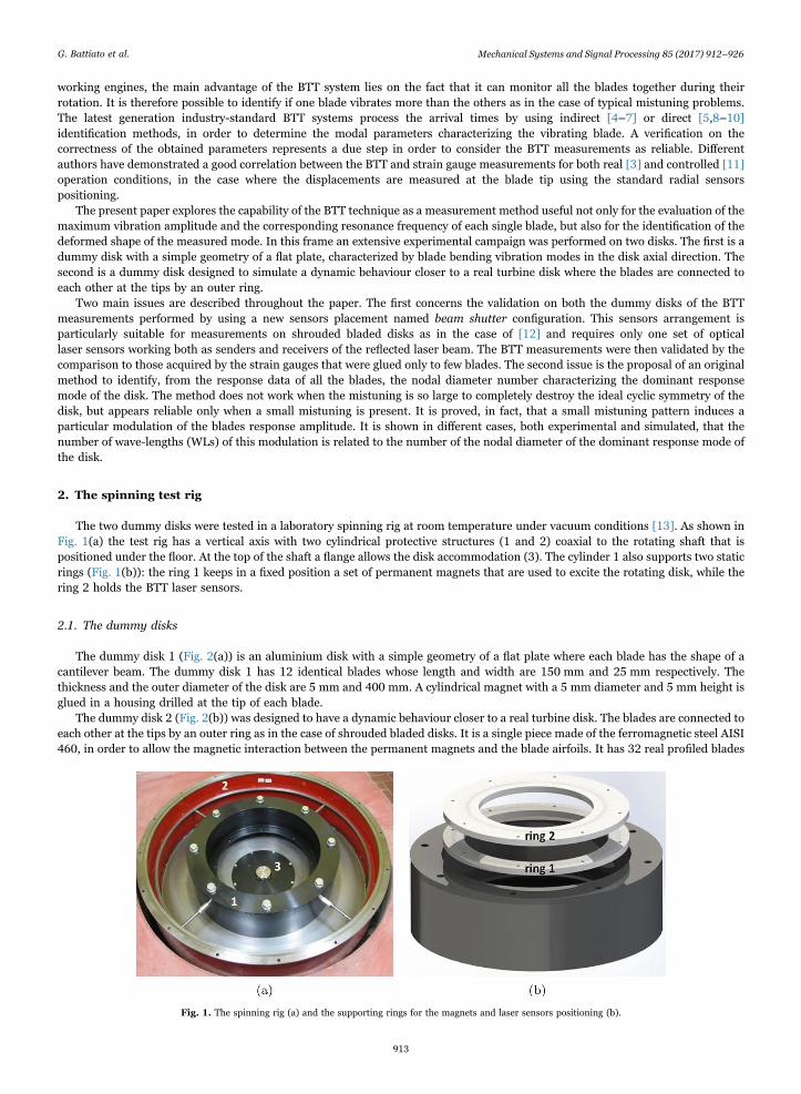
The two dummy disks were tested in a laboratory spinning rig at room temperature under vacuum conditions [13]. As shown inFig. 1(a) the test rig has a vertical axis with two cylindrical protective structures (1 and 2) coaxial to the rotating shaft that ispositioned under the floor. At the top of the shaft a flange allows the disk accommodation (3). The cylinder 1 also supports two staticrings (Fig. 1(b)): the ring 1 keeps in a fixed position a set of permanent magnets that are used to excite the rotating disk, while thering 2 holds the BTT laser sensors.

2.1. The dummy disks

The dummy disk 1 (Fig. 2(a)) is an aluminium disk with a simple geometry of a flat plate where each blade has the shape of acantilever beam. The dummy disk 1 has 12 identical blades whose length and width are 150 mm and 25 mm respectively. Thethickness and the outer diameter of the disk are 5 mm and 400 mm. A cylindrical magnet with a 5 mm diameter and 5 mm height isglued in a housing drilled at the tip of each blade.

The dummy disk 2 (Fig. 2(b)) was designed to have a dynamic behaviour closer to a real turbine disk. The blades are connected toeach other at the tips by an outer ring as in the case of shrouded bladed disks. It is a single piece made of the ferromagnetic steel AISI460, in order to allow the magnetic interaction between the permanent magnets and the blade airfoils. It has 32 real profiled blades

Fig. 1. The spinning rig (a) and the supporting rings for the magnets and laser sensors positioning (b).

G. Battiato et al. Mechanical Systems and Signal Processing 85 (2017) 912–926

913

whose length and aspect ratio are respectively 100 mm and 7.31. Its disk outer diameter and axial height are 630 mm and 20 mmrespectively.

2.2. The excitation system

The excitation system in the spinning test rig uses cylindrical permanent magnets (diameter 18 mm, height 10 mm, grade N52).The magnets are mounted in equally spaced positions on the static ring facing the rotating dummy disk (the ring 1 in Fig. 1(a)). Agraduated scale impressed on the ring 1 upper surface is used to fix the magnets at the right angular positions [13].

Several supporting rings with different inner diameters are available in order to guarantee the correct radial positioning of thepermanent magnets. Each magnet is glued on the tip of a screw that allows the regulation of the axial gap with respect to the diskblades. Six of the magnets were instrumented with force transducers for the measurement of the axial force exerted on the bladesduring the tests [13].

The number of magnets used in a specific test must be equal to the main engine order (EO) characterizing the excitationforce that should be simulated. The main engine order EOm

1 can be defined as the fist not-null harmonic index resulting from theFourier transform of the excitation force. In general for m equally spaced magnets, the EO pattern exciting the disk is defined asfollows:

i m iEO = · , ∀ = 1, 2, 3, …mi (1)

A mode shape of a bladed disk corresponding to a certain number of nodal diameters (NDs) can be excited by different EOsaccording to the following relationship, where Nb is the number of the disk's blades:

jN jEO = ± ND, ∀ = 0, 1, 2, 3, …b (2)

The excitation frequency is related both to the EO and to the rotational speed n by the following equation, where n is given in rpmand fexc in Hz:

f n= EO·60exc (3)

From Eq. (3) it can be noted that for increasing EO values a bladed disk can be excited at the same excitation frequency fexc for lowervalues of the rotational speed n.

2.3. The strain measurement system

The two dummy disks were instrumented by means of strain gauges. For both the disks the identification of the strain gaugepositions came out from their finite element (FE) modal analyses in cyclic symmetry conditions. Areas of high strains and low straingradients were identified as the best locations for strain gauges. The strain gauge signals were acquired through a telemetry system.

For the dummy disk 1 the strain gauges were attached at the two sides of the blade root (Fig. 3(a)). This position was chosen inorder to measure the out-of-plane (OOP) bending mode (1F) belonging to its first modal family. The strain gauges adopted arecomposed by a single grid of dimension 1. 52 mm × 3. 05 mm, with a grid resistance of 350 Ω. The two grids at the two sides of theblade were connected together with a half bridge. For the dummy disk 2 the strain gauge was applied on the back of a blade airfoil(Fig. 3(b)). The selected area was not affected by strain gradients for both the flap-restricted (1FR) and the torsional (1T) modeshapes belonging to its second and third modal families respectively. The strain gauges was a tee rosettes (grid resistance 350 Ω)composed by two separate grids (1.52 mm × 1.78 mm) with perpendicular axes that were connected together with a half bridge.During the dynamic tests the strain gauge signals were sampled with a sampling frequency of 8192 Hz and then post-processed usingthe following parameters:

Fig. 2. The dummy disk 1 (a) and the dummy disk 2 (b) within the spinning test rig.

G. Battiato et al. Mechanical Systems and Signal Processing 85 (2017) 912–926

914

• time width of each bin of samples for FFT analysis: 4 s;

• percentage of overlap between bins: 50%;

• ramp speed: 18.75 rpm/s.

The strain gauges measurement chain was verified by means of static tests on the dummy disk 1, which consisted in measuringthe bending strains at the blade root due to a set of calibrated masses positioned on its free end. For three static tests that wereperformed for three masses having different weights, the measured strains were compared to the corresponding numerical quantitiesdetermined by means of a static FE analysis. The results listed in Table 1 show the reliability of the strain gauges that can be used asa reference measurement system for the validation of the BTT technique.

Although the static measurement was repeated, only negligible differences were found between the experimental strains since thetest showed high repeatability.

3. The Blade Tip-Timing measurement system

The BTT technique employs a set of non-contact sensors mounted on the casing and facing the blades of a rotating bladed disk[1–3]. This technique is based on the measurement and the subsequent analysis of the difference between the Times-of-Arrival(ToA) of each vibrating blade passing by the sensors and the theoretical ToA of the non-vibrating blade [14]. From the post-processing of the collected ToA the dynamic properties of each blade, i.e. the resonance frequencies, the vibration amplitudes and themodal damping can be identified. The BTT has two main advantages over the strain gauges:

• it is a non-contact measurement system that does not affect the dynamic behaviour of the blades;

• it allows the measurement of all the blades of the disk, while the strain gauges are usually attached only to few blades.

The BTT system adopted in this study is a latest generation system that uses optical laser sensors. For the dummy disks 1 and 2all the tests were performed by employing five sensors for the direct detection of the blades ToA and an additional sensor ( rev1/sensor) measuring the rotational speed and representing the reference for all the others. The signal from the rev1/ sensor wasacquired by both the BTT and the strain gauge systems in order to synchronize the measured blade vibration signals during the post-processing operations.

3.1. The beam shutter method and the sensor positioning

The standard measurement approach for the BTT method is based on a set of sensors that are positioned along the radialdirection in order to detect the ToA at the blade tip where the maximum vibration amplitude occurs. Although this sensorpositioning is particularly suitable for disk with tip free blades, it is impracticable for shrouded bladed disks. In fact, due to the

Fig. 3. Strain gauge at the blade root of the dummy disk 1 (a) and strain gauge at the back of the airfoil of a dummy disk 2 blade (b).

Table 1Experimental and numerical strains for the static tests on the dummy disk 1.

Mass (kg) Experimental strain (μϵ) Numerical strain (μϵ)

0.76 130.23 130.191 169.30 169.271.99 342.32 342.25

G. Battiato et al. Mechanical Systems and Signal Processing 85 (2017) 912–926

915

presence of shrouds the laser sensors are not able to capture the motion at the tips. For this reason a new sensor configuration calledbeam shutter was tested on the two dummy disks introduced in Section 2.1. The sensors positioning adopted for the two cases ispresented in Fig. 4.

While the application of Fig. 4(a) tested the capabilities of the beam shutter configuration when the OOP vibration modes of theblades have to be detected (Section 5), the case of Fig. 4(b) clearly brings out the need to measure the vibrations at the blade trailingand leading edges since a direct detection of the vibrations at the blade tips cannot take place.

One of the attempts of using the BTT method to measure the blade vibrations at the trailing and leading edges makes use of thebeam interrupt configuration as shown in [12], where two sets of laser sensors, one acting as a sender of the laser beam and theother as a receiver, were employed within the flow path of a working engine. The configuration proposed in the present paper wouldovercome this inconvenient because in the case of real applications only one set of sender–receiver optical laser sensors areembedded in only one probe (Fig. 4). Since a smaller number of sensors is involved in the measurements, the beam shutter appearsmore robust and less invasive than the beam interrupt configuration.

For both the applications in Fig. 4 each sensor was mounted above the disk and produced a laser beam that was collimatedthrough a lens on a reflective tape stuck on a fixed surface beneath the disk. During the disk rotation the passing blade acts as ashutter, blocking the returning light towards the sender–receiver sensor. The system was set up in order to direct the laser beamtowards the leading and trailing edge locations where the blade experienced the maximum vibration amplitudes. The optical sensorsand the reflective tape were employed in measurements performed without any significant temperature variation from the roomtemperature. The maximum temperature at which the laser probes can work is 315 °C.

The sensors were installed at the same distance from the disk centre and their relative circumferential position was chosen inboth the cases by means of an optimization tool, which avoids the aliasing effect in the identification of the travelling wave modeshape characterizing the vibrating disk. The optimization tool requires as input the number of sensors, the expected engine ordersand the number of blades.

3.2. The Blade Tip-Timing data post-processing

The data were post-processed by using a fitting method called circumferential Fourier fit (CFF) [15]. This method requires threeor more sensors installed at the same chord-wise position. Assuming a certain response order, corresponding to the selected EO, foreach averaged rpm a sinusoidal wave is fitted to the data [5,8–10], in other words, each blade is assumed to vibrate according to asinusoidal wave. The equation of the blade motion seen by the kth sensor is:

y ω c A ω π f t Φ ω c A ω θ Φ ω( ) = + ( )·sin (2 ·EO· · + ( )) = + ( )·sin (EO· + ( ))k k (4)

where A ω( ) and Φ ω( ) are the amplitude of vibration and phase at a certain frequency ω and θk is the angular position of the kthsensor. For a given blade at each frequency (that is each value of the rotational speed) the displacement y ω( )k is measured by each ofthe kth sensor. Eq. (4) is then written for each sensor and the terms A ω( ), Φ ω( ) and c are calculated by a least square process if morethan 3 sensors are involved in the measurements. The amplitude A ω( ) can then be plotted versus the rotational speed as shown laterin Fig. 8.

4. The results comparison method

In order to verify the accuracy of the BTT method, the vibration parameters identified by the BTT were compared to thosedetected by the strain gauges in conjunction to the telemetry system. Simultaneous measurements with the BTT and the strain gaugesystems were performed for a certain set of vibrating modes characterizing the dummy disks. While the comparison in terms ofresonance frequencies is straightforward and requires a fast data processing, the comparison in terms of vibration amplitudes is amore demanding task. Indeed, it requires a preliminary FE modal analysis of the disks, since the strain gauges system measuresstrains (ϵSG), while the BTT measures displacements (uBTT).

Fig. 4. Beam shutter configuration for the dummy disk 1 (a) and the dummy disk 2 (b).

G. Battiato et al. Mechanical Systems and Signal Processing 85 (2017) 912–926

916

By the FE model the parameter K u= /ϵmod mod mod can be calculated, where:

• umod is the modal displacement of the node corresponding to the laser position on the blade in the same direction of thedisplacement detected by the BTT;

• ϵmod is the modal strain in the area corresponding to the strain gauges position in the same direction of the strain detected by thestrain gauges.

The same parameters can be defined for the physical measured quantities u (displacement of the blade at the BTT laser position) andϵ (strain at the strain gauges position) K u= /ϵphy . Since the two disks can be considered linear and their responses give well separatedmodes, the following relationship should be satisfied:

K K u K= ⇒ϵ

=phy mod mod (5)

The displacement of the blade corresponding to the strain measurement from Eq. (5) can be determined as:

u K= ·ϵSG mod SG (6)

Since the FE model was tuned previously by the strain gauge measurements (see Table 1) the obtained parameter uSG is consideredas reference for the displacement value measured by the BTT system uBTT.

5. Results on the dummy disk 1

In order to predict the natural frequencies and the mode shapes a FE dynamic calculation in cyclic symmetry conditions wasperformed. In Fig. 5(a) the natural frequencies of the dummy disk 1 are plotted against the respective NDs (FreND diagram)resulting in the first modal family called 1F.

Each black circle in Fig. 5(a) refers to an OOP bending mode of the blade when the disk vibrates according to a certain ND. Fromthe numerical Campbell diagram in Fig. 5(b) the rotational speeds at which the resonances occur can be estimated. The modescorresponding to ND=5 and ND=6 were chosen to be tested since they represent the different cases of rotating and standing modeshapes respectively [16]. Furthermore, in order to avoid high operation speeds the mode with ND=6 was excited by a harmonic forcewith EO=6 at 1951 rpm, while the mode with ND=5 was excited by a harmonic force with EO=7 (Eq. (2)) at 1356 rpm instead ofEO=5 at 1910 rpm.

5.1. Displacement measurement with the Blade Tip-Timing

The dummy disk 1 is excited in order to have OOP vibrations of the blades (the blade vibrates along the axial direction). In orderto operate in the beam shutter configuration in case of an OOP vibration of the blades, the sensors cannot be positioned with thelaser beam pointing along the radial direction. Indeed, in this case there is no tangential displacement of the blade that can produce adifferent ToA with respect to the non-vibrating blade ToA. For this reason the sensors can be positioned as shown in Fig. 4(a): eachsensor is tilted by an angle of 45° with respect to the plane containing the undeformed disk. This particular angle of the sensorsallows the BTT system to detect a ToA of the blade under the sensor that is not zero as shown by the scheme of the blade interruptingthe laser beam in Fig. 6. The time lag tΔ between the detected ToA and the theoretical ToA of the undeformed position ( tΔ in Fig. 6)is proportional to a fictitious tangential displacement vΔ of the blade that is equal to the actual axial displacement uΔ . For this reasonthe ToA can be used to calculate the blade axial displacement uΔ .

Fig. 5. Numerical FreND diagram for the dummy disk 1 (a) and numerical Campbell diagram for the dummy disk 1 (b).

G. Battiato et al. Mechanical Systems and Signal Processing 85 (2017) 912–926

917

5.2. Preliminary test

A preliminary rotating test was performed to identify the actual resonance frequencies. A single magnet was mounted on the testrig so that the disk could be excited simultaneously by means of an infinite number of harmonic excitations EO( = 1, 2, 3, …)1 . Thetest was planned in order to investigate the speed range 600–2600 rpm.

From the strain gauges time signal the experimental Campbell diagram (Fig. 7) was processed using Matlab. The naturalfrequencies for the modes corresponding to ND=5 and ND=6, which were determined by reading the y-axis values of the whitepoints, are listed in Table 2.

5.3. Test campaign on the dummy disk 1

The test campaign was performed for the modes that were excited by the EOs determined from Eq. (2) for j=1. A singlepermanent magnet was adopted for the excitation. A gap of 7 mm between the permanent magnet and those glued at the blades' tipswas set for all the tests. Strain and ToA were acquired simultaneously for two speed ranges including the values of nres at which theresonances occur. The main tests parameters are listed in Table 3.

The test campaign was repeated 3 times. For each test a linear sweep in speed with an acceleration of 18.75 rpm/s wasperformed.

5.4. The comparison BTT–strain gauges on the dummy disk 1

The strain gauges and BTT data were post-processed for each of the studied modes by using the same procedure employed in the

Fig. 6. Beam shutter working principle adopted for detecting the out of plane vibration modes for the dummy disk 1.

Fig. 7. Experimental Campbell diagram for the dummy disk 1.

G. Battiato et al. Mechanical Systems and Signal Processing 85 (2017) 912–926

918

preliminary test. The detected and derived displacements (uBTT and uSG) and the corresponding resonance frequencies wereaveraged over the three acquisitions. The values of fSG, fBTT, uSG and uBTT for the three separate acquisitions are reported inTable 4, where the high repeatability of the measurements can be noted.

The mean values of the previous frequencies and displacements at resonance are listed in Table 5 so that a direct comparisonbetween the two measurement systems can be carried out using the following relationships:

ef f

fe u u

u=

¯ −¯¯ ·100 = ¯ − ¯

¯·100f

SG BTT

SGu

SG BTT

SG (7)

where ef and eu are the percentage differences between the resonance frequencies and vibration amplitudes detected by the straingauges and the BTT respectively. From Table 5 it can be noted that the difference in terms of resonance frequency is negligible(e < 0.5%f ) while the difference in terms of resonance amplitude is less than 2% (e < 2%u ).

5.5. From a single blade measurement to the global disk response

One of the advantages of the BTT system over the strain gauges is that every blade can be measured while, if the strain gauges areused, only the response of the instrumented blades are detected. However, the measurement of the blades as independent structureshaving their own amplitude and resonance frequency does not allow to catch the global disk behaviour when a mode shape with acertain number ND of nodal diameters occurs. The estimation of the ND number of a bladed disk vibrating in resonance conditioncan be carried out with aid of a numerical Campbell diagram (e.g. similar to that of Fig. 5(b)), obtained from the FE model of thebladed disk. In particular, when a resonance is detected by the measurements, the corresponding rotational speed is the input valuefor the Campbell diagram to verify the presence of a crossing ND line–EO line that satisfies Eq. (2). Instead of estimating the NDnumber with the numerical Campbell diagram, it is here presented how it can be identified directly by the BTT measurements.

The forced responses of all the blades post-processed by the BTT for the studied mode shapes (ND=5 and ND=6) are plotted inFig. 8.

If the dummy disk was a perfectly tuned disk, i.e. all the hypotheses for a cyclic symmetric body were satisfied in terms ofgeometry, material properties and constraints, the forced response of each blade would be the same. It can be observed that thisholds for the standing operating deflection shape (ODS) with ND=6 (Fig. 8(a)), where the response peak of each blade occurs at thesame rotational speed with the same amplitude. This is not the case of the travelling ODS with ND=5 (Fig. 8(b)), where the maximaamplitudes occur at slightly different rotational speed and their envelope appears as a spatial wave along the blade number. Thesame spatial wave can be observed along the blade number at a given rotational speed.

This phenomenon was already observed in [17] where a test campaign on a non-rotating blisk excited by a set electromagnetsproducing an EO travelling force was performed. In that case it was demonstrated that, due to the presence of small mistuning of thedisk, the spatial wave resulting from the envelope of the blade peak amplitudes for a given excitation frequency had a number of

Table 2The dummy disk 1 resonance frequencies for the mode shapes with ND=5 and ND=6 (OOP bending modes).

EO (–) ND (–) nres (rpm) fres (Hz)

7 5 1356 158.26 6 1591 159.1

Table 3Test campaign for the dummy disk 1.

EO (–) ND (–) n-Range (rpm)

7 5 1300–14006 6 1550–1650

Table 4BTT and strain gauge measurements for the three tests on the dummy disk 1: the OOP vibration (1F) of the blades corresponding to ND=5 and ND=6 were detected.

Test (–) ND (–) Mode (–) fSG (Hz) fBTT (Hz) uSG (μm) uBTT (μm)

1 5 1F 158.10 159.80 1657.66 1651.502 5 1F 157.90 157.70 1669.50 1611.813 5 1F 158.00 156.50 1659.53 1631.13

1 6 1F 160.00 161.90 2314.57 2293.212 6 1F 160.00 159.80 2296.27 2289.213 6 1F 157.90 158.90 2285.41 2244.38

G. Battiato et al. Mechanical Systems and Signal Processing 85 (2017) 912–926

919

wavelenghts (WL, see Fig. 8) equal to two times the number of the ODS nodal diameters. In detail, for a dummy bladed disk with 24blades, four WLs were observed for an ODS with ND=2 and six WLs were observed for an ODS with ND=3. In the case of Fig. 8(b),where the ODS with ND=5 is shown, 10 WLs are expected. As it is shown in the same figure, the envelope of the maxima amplitudesclearly shows two WLs instead of ten. This is due to the aliasing effect generated by the poor resolution of a spatial wave with 10 WLsdiscretized by 12 blades only. In detail, assuming Nb as the number of blades,Wexp the number of WLs of the expected spatial waveand Ws the number of WLs of the spatial wave sampled by the blades, two cases can occur:

• if W N≤ /2exp b , the modulated spatial wave can be well recognized as a wave with Wexp wavelenghts. In this case W W=exp s and noaliasing occurs;

• ifW N> /2exp b (Fig. 8(b)), the number of blades is not large enough to correctly discretize a spatial wave withWexp wavelenghts. Inthis case aliasing occurs and the observed spatial wave has a number of wavelenghtsWs which satisfies the following relationship:

W jN W j= ± , ∀ = 0, 1, 2, 3, …exp b s (8)

In order to confirm the experimental observation in a simpler case where no aliasing occurs, the measurement was performedalso in the range of the natural frequency corresponding to ND=3: the ODS, plotted in Fig. 9, shows as expected a spatial wave withsix WLs.

In the next section a simplified lumped parameters system is used to explain the reason why the spatial wave is characterized by anumber of WLs that is twice the number of the ND of the travelling response.

5.6. An analytical model to explain the blade row response

The relationship between the number of WLs and the number ND is strictly associated to the existence of two repeated modes inthe presence of small mistuning. Repeated modes occur for N1 < ND < /2b if Nb is even. When ND=0 or ND=Nb/2 (for an evennumber of blades) only one mode is present and the spatial wave does not appear. This is confirmed by the observation of the flatODS corresponding to NND = /2 = 6b (Fig. 8(a)).

In order to explain the appearance of the spatial wave, a simple analytical model of a lumped parameter disk is used. The disk has12 sectors, each one with one degree of freedom coupled by means of springs to the neighbour sectors. The sectors are equal,therefore the disk is tuned and 12 identical forced response amplitudes are obtained as shown in Fig. 10(a) when the mode shapewith ND=3 is excited.

In Fig. 10(b) the two repeated mode shapes multiplied by their participation factors are plotted at resonance for different timeinstants. Under a travelling excitation the repeated mode shapes are orthogonal not only in space but also in time. The orthogonalityalong the blade number is clearly visible, while the orthogonality in time is indicated with the two black solid lines: when the firstmode is at its maximum amplitude the second mode is at its neutral position. The linear combination of the two modes produces a

Table 5BTT–strain gauge measurements comparison on the dummy disk 1.

ND (–) fSG (Hz) fBTT (Hz) ef (%) uSG (μm) uBTT (μm) eu (%)

5 158.0 158.0 0 1662.23 1631.48 1.886 159.3 160.2 0.44 2298.75 2275.60 1.02

Fig. 8. Experimental forced responses for the 12 blades of the dummy disk 1 detected by the BTT in the case of ND=6 (a) and ND=5 (b) mode shape.

G. Battiato et al. Mechanical Systems and Signal Processing 85 (2017) 912–926

920

travelling ODS (lowest subplot of Fig. 10(b)). Since the disk is tuned, the peak envelope of the blade amplitudes is a straight spatialline (red).

A random mistuning was then added to the disk model in terms of mass perturbation that causes a split of the repeated modesnatural frequencies fΔ of about 0.7% of the tuned natural frequencies. As it can be seen in Fig. 11(a), the consequence is that the sumof the two modes, having slightly different frequencies and amplitudes, gives an ODS where the peak envelope is a spatial wave withsix WLs for a ND=3 response as they appear in Fig. 9.

By using the same mistuned model the cases of Fig. 8(a) and (b) can also be simulated. Fig. 12(a) shows the simulated forcedresponses corresponding to the experimental case of Fig. 8(a), where a mode with ND=6 is excited. It can be seen in the simulation(Fig. 12(b)) that the second mode does not exist since the mode is standing and then it cannot give rise to a spatial wave.

Fig. 13(a) shows the result of the simulation for an ODS with ND=5. This example corresponds to the experimental case ofFig. 8(b). It can be seen that the simulated forced responses shows a modulated spatial wave with two WLs due to aliasing as in theexperiments. It can then be concluded that the presence of small mistuning, which is expected to be present in the real disks, can beuseful to experimentally identify the nodal diameters number.

6. Results on the dummy disk 2

The dummy disk 2 was created to reproduce a bladed disk dynamics similar to that of a real turbine disk. The measurements onthis disk allow testing the capability of the BTT system in the beam shutter configuration even on a disk with a more complexdynamics. The FE dynamic calculation on the dummy disk 2 showed that the modes belonging to the first three modal families arecharacterized by the flap (1F), flap restricted (1FR) and torsional (1T) mode shape of the blade. The FreND diagram correspondingto the 1st, 2nd and 3rd modal family is shown in Fig. 14. From the FE analyses on the dummy disk 2 the high strain locations on theblade airfoil, both for the 1FR and 1T mode shapes, were chosen for the strain gauges installation (Fig. 3(b)).

Fig. 9. Experimental forced responses for the 12 blades of the dummy disk 1 detected by the BTT in the case of the ND=3 mode shape.

Fig. 10. Numerical forced responses (a) and ODS (b) for a cyclic symmetric mode shape with ND=3. (For interpretation of the references to colour in this figurecaption, the reader is referred to the web version of this paper.)

G. Battiato et al. Mechanical Systems and Signal Processing 85 (2017) 912–926

921

Fig. 11. Numerical forced responses (a) and ODS (b) for a mistuned mode shape with ND=3.

Fig. 12. Numerical forced responses (a) and ODS (b) for a mistuned mode shape with ND=6.

Fig. 13. Numerical forced responses (a) and ODS (b) for a mistuned mode shape with ND=5.

G. Battiato et al. Mechanical Systems and Signal Processing 85 (2017) 912–926

922

6.1. Preliminary hammer test

A preliminary hammer test was performed to detect the modal parameters of the disk in static conditions (not rotating). In orderto have the same constraints with the shaft as during the rotation, the disk was kept mounted on the spinning rig during the hammertest. The response of each blade was measured by a laser scanner at the same location where the BTT laser sensors detect the bladevibrations.

It was observed that the cleanest disk responses for both the 1FR and 1T modes occurred for ND=7 at 1029 Hz and 1402 Hzrespectively. In Fig. 15 an example of the response processed by the laser scanner is shown. Considering these preliminary results, itwas chosen to compare the BTT and the strain gauges measurements when the disk was excited in rotating conditions to vibrateaccording the modal families 1FR and 1T for ND=7.

6.2. Test campaign on the dummy disk 2

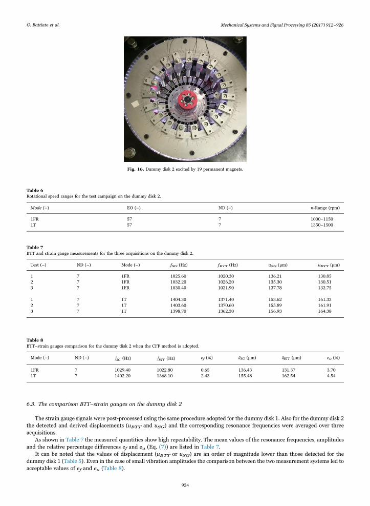
According to Eq. (2), considering that the number of blades is N = 32b and assuming j=2, it can be deduced that the mode withND=7 can be excited by an excitation with EO=57. Moreover, assuming i=3, from Eq. (1) it can be derived that a number of 19equally spaced magnets (m=19) facing the rotating disk can produce an excitation with EO=57. The test campaign was thenperformed with 19 permanent magnets (Fig. 16) at a gap of 5 mm from the blade leading edges. This produces in the disk a travellingexcitation with EO = 5719

3 that into a suitable speed range excites the modes at ND=7.The main test parameters are listed in Table 6. Strain and displacement were acquired simultaneously for 2 speed ranges

(Table 6) including the values of nres at which the resonances occur. For each test a linear speed sweep with an acceleration of18.75 rpm/s was performed. As in the case of the dummy disk 1 the test campaign was repeated 3 times.

Fig. 14. Numerical FreND diagram for the dummy disk 2.

Fig. 15. Hammer test on dummy disk 2: 1FR mode identification.

G. Battiato et al. Mechanical Systems and Signal Processing 85 (2017) 912–926

923

6.3. The comparison BTT–strain gauges on the dummy disk 2

The strain gauge signals were post-processed using the same procedure adopted for the dummy disk 1. Also for the dummy disk 2the detected and derived displacements (uBTT and uSG) and the corresponding resonance frequencies were averaged over threeacquisitions.

As shown in Table 7 the measured quantities show high repeatability. The mean values of the resonance frequencies, amplitudesand the relative percentage differences ef and eu (Eq. (7)) are listed in Table 7.

It can be noted that the values of displacement (uBTT or uSG) are an order of magnitude lower than those detected for thedummy disk 1 (Table 5). Even in the case of small vibration amplitudes the comparison between the two measurement systems led toacceptable values of ef and eu (Table 8).

Fig. 16. Dummy disk 2 excited by 19 permanent magnets.

Table 6Rotational speed ranges for the test campaign on the dummy disk 2.

Mode (–) EO (–) ND (–) n-Range (rpm)

1FR 57 7 1000–11501T 57 7 1350–1500

Table 7BTT and strain gauge measurements for the three acquisitions on the dummy disk 2.

Test (–) ND (–) Mode (–) fSG (Hz) fBTT (Hz) uSG (μm) uBTT (μm)

1 7 1FR 1025.60 1020.30 136.21 130.852 7 1FR 1032.20 1026.20 135.30 130.513 7 1FR 1030.40 1021.90 137.78 132.75

1 7 1T 1404.30 1371.40 153.62 161.332 7 1T 1403.60 1370.60 155.89 161.913 7 1T 1398.70 1362.30 156.93 164.38

Table 8BTT–strain gauges comparison for the dummy disk 2 when the CFF method is adopted.

Mode (–) ND (–) fSG (Hz) fBTT (Hz) ef (%) uSG (μm) uBTT (μm) eu (%)

1FR 7 1029.40 1022.80 0.65 136.43 131.37 3.701T 7 1402.20 1368.10 2.43 155.48 162.54 4.54

G. Battiato et al. Mechanical Systems and Signal Processing 85 (2017) 912–926

924

6.4. Nodal diameter identification on the dummy disk 2

The forced responses obtained for the mode 1T on each blade of the dummy disk 2 are plotted in Fig. 17(a).Although the small vibration amplitudes led to a set of noisy data collected by the BTT sensors, it can however be observed that

also in this case the phenomenon of the spatial wave can still be present as highlighted in Fig. 17(b). The shape of the WLs is in thiscase quite irregular, but it is still possible to recognize a modulated spatial wave with 14 peaks. In this case 14 peaks are expectedsince the excited travelling response is characterized by a number of nodal diameter ND=7.

The observation of this phenomenon is confirmed by other tests. An excitation with EO=19 is produced by 19 magnets.According to Eq. (2), considering the number of blades (N = 32b ) and j=1, the engine order EO=19 excites the mode with ND=13.The envelope of the maxima amplitudes of the forced responses in this case is that of Fig. 18(a) where six WLs are visible. In this casethe presence of six WLs instead of the expected 26 can be justified by Eq. (8) since the aliasing occurs. In fact, the number 26 of theexpected WLs of the spatial waves is higher than Nb/2. For the aliasing the visible number of WLs is six (32 − 26=6).

In order to confirm the results in one case where the aliasing phenomenon is not present, the measurement was repeated with 5magnets. According to Eq. (1) 5 magnets produce on the blades a set of travelling forces characterized by EO = 15, 30, 45, …15 . Inparticular, the measurement was performed considering an excitation corresponding to EO=30 in order to excite, according to Eq.(2), the mode shape with ND=2. The envelope of the maxima amplitudes of the forced responses in this case is that of Fig. 18(b)where four WLs, as expected, are visible since the aliasing is not present.

7. Conclusions

In this paper a BTT system with a new concept of sensors positioning was tested on two dummy disks (dummy disk 1 and dummydisk 2). The dummy disk 1 has a simple flat geometry and its blades show in resonance high displacement amplitudes (1600–2300 μm). The dummy disk 2 is more similar to a real turbine disk and it is characterized by families of modes close to each others.

Fig. 17. Experimental measurements on the dummy disk 2 (Nb=32) by the BTT, mode shape with ND=7 mode. (a) Forced responses of all the blades, (b) spatialwave.

Fig. 18. Envelope of the maxima amplitudes of the experimental forced responses (spatial waves) for the dummy disk 2 (Nb=32). Mode shape with ND=13 (a) andND=2 (b).

G. Battiato et al. Mechanical Systems and Signal Processing 85 (2017) 912–926

925

Two key features were here presented. First, a new measurement configuration for the optical probes of a BTT system, the beamshutter configuration, was tested by comparing the BTT with the strain gauge measurements. The beam shutter configuration provedto work properly since it gives the expected collection of measured data from the ToA of each blade under each sensor. In the case ofthe dummy disk 1, for the selected modes, high vibration amplitudes (1600–2300 μm) were found with an accuracy less than 2%with respect to the strain gauge measurements. For the dummy disk 2 the vibration amplitudes for the measured modes (130–150 μm) were smaller than that in the case of the previous disk. Even if the small amplitude values led to a set of noisy BTT data, theaccuracy with respect to the strain gauge measurements was still high (differences less than 5%). These results give confidence in thisnew way of positioning the optical probes. Second, a novel method to experimentally identify the nodal diameter number of thedetected mode is proposed. The method takes advantage from the availability of the forced responses of all the blades that is typicalof the processed BTT measurements. The method works when the detected mode is quite isolated from the others and in presence ofsmall mistuning. It does not work when the mistuning is large enough to completely decouple the blade row and destroy the idealcyclic symmetry of the disk. It was proved that a small mistuning produces a spatial wave modulating the vibration amplitude of theblade row. It was then shown that the number of nodal diameter related to the dominant mode can be identified starting from thenumber of WLs of this modulation.

Acknowledgements

The work described in this paper has been developed within the GREAT 2020-2 project funded by the Aerospace districtPiemonte, co-founded by the European POR-FESR 2007-2013.

References

[1] M. Zielinski, G. Ziller, Noncontact vibration measurements on compressor rotor blades, Meas. Sci. Technol. 11 (7) (2000) 847.[2] Ye I. Zablotskiy, Yu A. Korostelev, Measurement of resonance vibrations of turbine blades with the ELURA device, Energomashinostroneniye (USSR) 2 (1970)

36–39.[3] Michael Zielinski, Gerhard Ziller, Noncontact blade vibration measurement system for aero engine application, in: 17th International Symposium on

Airbreathing Engines, 2005.[4] S. Heath, M. Imregun, An improved single-parameter tip-timing method for turbomachinery blade vibration measurements using optical laser probes, Int. J.

Mech. Sci. 38 (10) (1996) 1047–1058.[5] G. Dimitriadis, I.B. Carrington, J.R. Wright, J.E. Cooper, Blade-tip timing measurement of synchronous vibrations of rotating bladed assemblies, Mech. Syst.

Signal Process. 16 (4) (2002) 599–622.[6] S. Heath, M. Imregun, A survey of blade tip-timing measurement techniques for turbomachinery vibration, J. Eng. Gas Turbines Power 120 (4) (1998)

784–791.[7] S. Heath, A new technique for identifying synchronous resonances using tip-timing, J. Eng. Gas Tubines Power ASME 122 (2000) 219–224.[8] I.B. Carrington, J.R. Wright, J.E. Cooper, G. Dimitriadis, A comparison of blade tip timing data analysis methods, Proc. Inst. Mech. Eng. Part G: J. Aerosp. Eng.

215 (5) (2001) 301–312.[9] J. Gallego-Garrido, G. Dimitriadis, J.R. Wright, A class of methods for the analysis of blade tip timing data from bladed assemblies undergoing simultaneous

resonances – Part I: theoretical development, Int. J. Rotat. Mach. 2007 (2007).[10] J. Gallego-Garrido, G. Dimitriadis, J.R. Wright, A class of methods for the analysis of blade tip timing data from bladed assemblies undergoing simultaneous

resonances – Part II: experimental validation, Int. J. Rotat. Mach. 2007 (2007).[11] D. Knappett, J. Garcia, Blade tip timing and strain gauge correlation on compressor blades, Proc. Inst. Mech. Eng. Part G: J. Aerosp. Eng. 222 (4) (2008)

497–506.[12] Michael Zielinski, Vibration measurements on compressor blades and shrouded turbine blades, in: 14th Blade Mechanics Seminar, 2009.[13] T. Berruti, V. Maschio, P. Calza, Experimental investigation on the forced response of a dummy counter-rotating turbine stage with friction damping, J. Eng.

Gas Turbines Power 134 (12) (2012) 122502.[14] Michael Zielinski, Gerhard Michael, Noncontact Blade Vibration Measurement System For Aero Engine Application, 2005.[15] Hood Technology, Analyze Blade Vibration User Manual, ver 7.5, February 2014.[16] D.L. Thomas, Dynamics of rotationally periodic structures, Int. J. Numer. Methods Eng. 14 (1) (1979) 81–102.[17] C.M. Firrone, T. Berruti, An electromagnetic system for the non-contact excitation of bladed disks, Exp. Mech. 52 (5) (2012) 447–459.

G. Battiato et al. Mechanical Systems and Signal Processing 85 (2017) 912–926

926

本文献由“学霸图书馆-文献云下载”收集自网络，仅供学习交流使用。

学霸图书馆（www.xuebalib.com）是一个“整合众多图书馆数据库资源，

提供一站式文献检索和下载服务”的24 小时在线不限IP

图书馆。

图书馆致力于便利、促进学习与科研，提供最强文献下载服务。

图书馆导航：

图书馆首页 文献云下载 图书馆入口 外文数据库大全 疑难文献辅助工具