forecasting biodiversity in breeding birds using best ... · considering the forecast horizon ......
TRANSCRIPT

Submitted 19 September 2017Accepted 29 December 2017Published 8 February 2018
Corresponding authorDavid J Harrisdaveharris-researchme
Academic editorJames Roper
Additional Information andDeclarations can be found onpage 21
DOI 107717peerj4278
Copyright2018 Harris et al
Distributed underCreative Commons CC-BY 40
OPEN ACCESS
Forecasting biodiversity in breeding birdsusing best practicesDavid J Harris1 Shawn D Taylor2 and Ethan P White134
1Department of Wildlife Ecology and Conservation University of Florida Gainesville FLUnited States of America
2 School of Natural Resources and Environment University of Florida Gainesville FLUnited States of America
3 Informatics Institute University of Florida Gainesville FL United States of America4Biodiversity Institute University of Florida Gainesville FL United States of America
ABSTRACTBiodiversity forecasts are important for conservationmanagement and evaluating howwell current models characterize natural systems While the number of forecasts forbiodiversity is increasing there is little information available on howwell these forecastswork Most biodiversity forecasts are not evaluated to determine how well they predictfuture diversity fail to account for uncertainty and do not use time-series data thatcaptures the actual dynamics being studied We addressed these limitations by usingbest practices to explore our ability to forecast the species richness of breeding birds inNorth America We used hindcasting to evaluate six different modeling approachesfor predicting richness Hindcasts for each method were evaluated annually for adecade at 1237 sites distributed throughout the continental United States All modelsexplained more than 50 of the variance in richness but none of them consistentlyoutperformed a baseline model that predicted constant richness at each site The bestpractices implemented in this study directly influenced the forecasts and evaluationsStacked species distribution models and lsquolsquonaiversquorsquo forecasts produced poor estimates ofuncertainty and accounting for this resulted in these models dropping in the relativeperformance compared to other models Accounting for observer effects improvedmodel performance overall but also changed the rank ordering of models because itdid not improve the accuracy of the lsquolsquonaiversquorsquo model Considering the forecast horizonrevealed that the prediction accuracy decreased across all models as the time horizonof the forecast increased To facilitate the rapid improvement of biodiversity forecastswe emphasize the value of specific best practices in making forecasts and evaluatingforecasting methods
Subjects Ecology Data Mining and Machine Learning Climate Change BiologyKeywords Birds Breeding bird survey Species richness Biodiversity Forecasting PredictionClimate change Species distribution model Time series Space-for-time substitution
INTRODUCTIONForecasting the future state of ecological systems is increasingly important for planning andmanagement and also for quantitatively evaluating how well ecological models capture thekey processes governing natural systems (Clark et al 2001 Dietze et al 2018 Houlahan etal 2017) Forecasts regarding biodiversity are especially important due to biodiversityrsquos
How to cite this article Harris et al (2018) Forecasting biodiversity in breeding birds using best practices PeerJ 6e4278 DOI107717peerj4278
central role in conservation planning and its sensitivity to anthropogenic effects (Cardinaleet al 2012 Diacuteaz et al 2015 Tilman et al 2017) High-profile studies forecasting largebiodiversity declines over the coming decades have played a large role in shapingecologistsrsquo priorities (as well as those of policymakers eg IPCC 2014) but it is inherentlydifficult to evaluate such long-term predictions before the projected biodiversity declineshave occurred
Previous efforts to predict future patterns of species richness and diversity moregenerally have focused primarily on building species distributions models (SDMs Thomaset al 2004 Thuiller et al 2011 Urban 2015) In general these models describe individualspeciesrsquo occurrence patterns as functions of the environment Given forecasts for environ-mental conditions these models can predict where each species will occur in the futureThese species-level predictions are then combined (lsquolsquostackedrsquorsquo) to generate forecasts forspecies richness (egCalabrese et al 2014) Alternatively models that directly relate spatialpatterns of species richness to environmental conditions have been developed and generallyperform equivalently to stacked SDMs (Algar et al 2009 Distler Schuetz amp Langham2015) This approach is sometimes referred to as lsquolsquomacroecologicalrsquorsquo modeling becauseit models the larger-scale pattern (richness) directly (Distler Schuetz amp Langham 2015)
Despite the emerging interest in forecasting species richness and other aspects ofbiodiversity (Jetz Wilcove amp Dobson 2007 Thuiller et al 2011) little is known about howeffectively we can anticipate these dynamics This is due in part to the long time scales overwhichmany ecological forecasts are applied (and the resulting difficulty in assessingwhetherthe predicted changes occurred Dietze et al 2018) What we do know comes from a smallnumber of hindcasting studies where models are built using data on species occurrenceand richness from the past and evaluated on their ability to predict contemporary patterns(eg Algar et al 2009 Distler Schuetz amp Langham 2015) or historic (Blois et al 2013Maguire et al 2016) periods not used for model fitting These studies are a valuable firststep but lack several components that are important for developing forecasting modelswith high predictive accuracy and for understanding how well different methods canpredict the future These lsquolsquobest practicesrsquorsquo for effective forecasting and evaluation (Box 1)broadly involve (1) expanding the use of data to include biological and environmentaltime-series (Tredennick et al 2016) (2) accounting for uncertainty in observations andprocesses (Yu Wong amp Hutchinson 2010 Harris 2015) and (3) conducting meaningfulevaluations of the forecasts by hindcasting archiving short-term forecasts and comparingforecasts to baselines to determine whether the forecasts are more accurate than assumingthe system is basically static (Dietze et al 2018)
In this paper we attempt to forecast the species richness of breeding birds at over 1200of sites located throughout North America while following best practices for ecologicalforecasting (Box 1) To do this we combine 32 years of time-series data on bird distributionsfrom annual surveys with monthly time-series of climate data and satellite-based remote-sensing Contemporary datasets that span a time scale of 30 years or more have onlyrecently become available for large-scale time-series based forecasting A dataset of this sizeallows us to model and assess changes a decade or more into the future in the presenceof shifts in environmental conditions on par with predicted climate change We compare
Harris et al (2018) PeerJ DOI 107717peerj4278 227
Figure 1 Example predictions from six forecasting models for a single site Data from 1982 through2003 connected by solid lines were used for training the models the remaining points were used forevaluating the modelsrsquo forecasts In each panel point estimates for each year are shown with lines thedarker ribbon indicates the 68 prediction interval (one standard deviation of uncertainty) and thelighter ribbon indicates the 95 prediction interval (A) Single-site models were trained independently oneach sitersquos observed richness values The first two models (lsquolsquoaveragersquorsquo and lsquolsquonaiversquorsquo) served as baselines (B)The environmental models were trained to predict richness based on elevation climate and NDVI theenvironmental modelsrsquo predictions change from year to year as environmental conditions change
Full-size DOI 107717peerj4278fig-1
traditional distribution modeling based approaches to spatial models of species richnesstime-series methods and two simple baselines that predict constant richness for each siteon average (Fig 1) All of our forecasting models account for uncertainty and observationerror are evaluated across different time lags using hindcasting and are publicly archivedto allow future assessment We discuss the implications of using best practices for ourunderstanding of and confidence in the resulting forecasts and how we can continue tobuild on these approaches to improve ecological forecasting in the future
METHODSWe evaluated six types of forecasting models (Table 1) by dividing the 32 years of data into22 years of training data and 10 years of data for evaluating forecasts using hindcastingHere we use definitions from meteorology where a hindcast is generally any prediction foran event that has already happened while forecasts are predictions for actual future events(Jolliffe amp Stephenson 2003) We also made long term forecasts by using the full data setfor training and making forecasts through the year 2050 For both time frames we made
Harris et al (2018) PeerJ DOI 107717peerj4278 327
Table 1 Six forecasting models Single-site models were trained site-by-site without environmental dataEnvironmental models were trained using all sites together without information regarding which tran-sects occurred at which site or during which year Most of the models were trained to predict richness di-rectly This mirrors the standard application of these techniques Separate random forest SDMs were fitfor each species and used to predict the probability of that species occurring at each site The species-levelprobabilities at a site were summed to predict richness The mistnet JSDM was trained to predict the fullspecies composition at each site and the number of species in its predictions was used as an estimate ofrichness
Predictors
Model Response variable Site id Time Environment
Single-site modelsAverage baseline richness X
Naive baseline richness X X
Auto-ARIMA richness X X
Environmental modelsGBM richness richness X
Stacked SDMs species-level presence X
Mistnet JSDM species composition X
forecasts using each model with and without correcting for observer effects as describedbelow
DataRichness dataBird species richness was obtained from the North American Breeding Bird Survey (BBS)(Pardieck et al 2017) using the Data Retriever Python package (Morris amp White 2013Senyondo et al 2017) and rdataretriever R package (McGlinn et al 2017) BBS observationsare three-minute point counts made at 50 fixed locations along a 40 km route Here wedenote each route as a site and summarize richness as the total number of species observedacross all 50 locations in each surveyed year The data was filtered to exclude all nocturnalcepuscular and aquatic species (since these species are not well sampled by BBS methodsHurlbert amp White 2005) as well as unidentified species and hybrids All data from surveysthat did not meet BBS quality criteria were also excluded
We used observed richness values from 1982 (the first year of complete environmentaldata) to 2003 to train the models and from 2004 to 2013 to test their performance We onlyused BBS routes from the contiguous United States (ie routes where climate data wasavailable PRISM Climate Group (2004)) and we restricted the analysis to routes that weresampled during 70 of the years in the training period (ie routes with at least 16 annualobservations) The resulting dataset included 34494 annual surveys of 1279 unique sitesand included 385 species Site-level richness varied from 8 to 91 with an average richnessof 51 species
Past environmental dataEnvironmental data included a combination of elevation bioclimatic variables and aremotely sensed vegetation index (the normalized difference vegetation index NDVI)
Harris et al (2018) PeerJ DOI 107717peerj4278 427
all of which are known to influence richness and distribution in the BBS data (Kent Bar-Massada amp Carmel 2014 Hurlbert amp Haskell 2002) For each year in the dataset we usedthe 4 km resolution PRISMdata (PRISM Climate Group 2004) to calculate eight bioclimaticvariables identified as relevant to bird distributions (Harris 2015) mean diurnal rangeisothermality max temperature of the warmest month mean temperature of the wettestquarter mean temperature of the driest quarter precipitation seasonality precipitationof the wettest quarter and precipitation of the warmest quarter These variables werecalculated for the 12 months leading up to the annual survey (JulyndashJune) as opposed to thecalendar year Satellite-derived NDVI a primary correlate of richness in BBS data (Hurlbertamp Haskell 2002) was obtained from the NDIV3g dataset with an 8 km resolution (Pinzonamp Tucker 2014) and was available from 1981ndash2013 Average summer (April May June)and winter (December January Feburary) NDVI values were used as predictors Elevationwas from the SRTM 90m elevation dataset (Jarvis et al 2008) obtained using the R packageraster (Hijmans 2016) Because BBS routes are 40-km transects rather than point countswe used the average value of each environmental variable within a 40 km radius of eachBBS routersquos starting point
Future environmental projectionsIn addition to the analyses presented here we have also generated and archived long termforecasts from 2014ndash2050 This will allow future researchers to assess the performanceof our six models on longer time horizons as more years of BBS data become availablePrecipitation and temperature were forecast using the CMIP5 multi-model ensembledataset (Brekke et al 2013) Thirty-seven downscaled model runs (Brekke et al 2013 seeTable S1) using the RCP60 scenario were averaged together to create a single ensemble usedto calculate the bioclimatic variables for North America For NDVI we used the per-siteaverage values from 2000ndash2013 as a simple forecast For observer effects (see below) eachsite was set to have zero observer bias The predictions have been archived on Zenodo(Harris White amp Taylor 2017b)
Accounting for observer effectsObserver effects are inherent in large data sets collected by different observers and areknown to occur in BBS (Sauer Peterjohn amp Link 1994) For each forecasting approachwe trained two versions of the corresponding model one with corrections for differencesamong observers and one without (Fig 2) We estimated the observer effects (andassociated uncertainty about those effects) using a linear mixed model with observeras a random effect built in the Stan probabilistic programming language (Carpenter etal 2017) Because observer and site are strongly related (observers tend to repeatedlysample the same site) site-level random effects were included to ensure that inferreddeviations were actually observer-related (as opposed to being related to the sites that agiven observer happened to see) The resulting model is described mathematically andwith code in Supplemental Information 2 The model partitions the variance in observedrichness values into site-level variance observer-level variance and residual variance (egvariation within a site from year to year)
Harris et al (2018) PeerJ DOI 107717peerj4278 527
Figure 2 (A) Model predictions for Pennsylvania route 35 when all observers are treated the same(black points) (B) Model predictions for the same route when accounting for systematic differences be-tween observers (represented by the pointsrsquo colors) In this example most models are made more robustto observer turnover Note that the lsquolsquonaiversquorsquo model is less sensitive to observer turnover and does not ben-efit as much from modeling it
Full-size DOI 107717peerj4278fig-2
Across our six modeling approaches (described below) we used estimates from theobserver model in three different ways First the expected values for site-level richnesswere used directly as our lsquolsquoaveragersquorsquo baseline model (see below) For the two models thatmade species-level predictions the estimated observer effects were included alongside theenvironmental variables as predictors Finally we trained the remaining models to predictobserver-corrected richness values (ie observed richness minus the observer effect orthe number of species that would have been recorded by a lsquolsquotypicalrsquorsquo observer) Since thesite-level and observer-level random effects are not known precisely we represented therange of possible values using 500 Monte Carlo samples from the posterior distributionover these effects Each downstream model was then trained 500 times using differentpossible values for the random effects
Models site-level modelsThree of themodels used in this study were fit to each site separately with no environmentalinformation (Table 1) These models were fit to each BBS route twice once using theresiduals from the observermodel and once using the raw richness valuesWhen correcting
Harris et al (2018) PeerJ DOI 107717peerj4278 627
for observer effects we averaged across 500models that were fit separately to the 500MonteCarlo estimates of the observer effects to account for our uncertainty in the true valuesof those effects All of these models use a Gaussian error distribution (rather than a countdistribution) for reasons discussed below (see lsquolsquoModel evaluationrsquorsquo)
Baseline modelsWe used two simple baseline models as a basis for comparison with the more complexmodels (Fig 1 Table 1) The first baseline called the lsquolsquoaveragersquorsquo model treated site-levelrichness observations either as uncorrelated noise around a site-level constant
yt =micro+εt
Predictions from the lsquolsquoaveragersquorsquo model are thus centered on micro which could either be themean of the raw training richness values or an output from the observer model Thismodelrsquos confidence intervals have a constant width that depends on the standard deviationof ε which can either be the standard deviation of the raw training richness values orσ residual from the observer model see Supplemental Information 2)
The second baseline called the lsquolsquonaiversquorsquo model (Hyndman amp Athanasopoulos 2014) wasa simple autoregressive process with a single year of history ie an ARIMA(010) model
y=ytminus1+εt
where the standard deviation of ε is a free parameter for each site In contrast to thelsquolsquoaveragersquorsquo model whose predictions are based on the average richness across the wholetime series the lsquolsquonaiversquorsquo model predicts that future observations will be similar to the finalobserved value (eg in our hindcasts the value observed in 2003) Moreover because theε values accumulate over time the confidence intervals expand rapidly as the predictionsextend farther into the future Despite these differences both modelsrsquo richness predictionsare centered on a constant value so neither model can anticipate any trends in richness orany responses to future environmental changes
Time series modelsWe used Auto-ARIMA models (based on the autoarima function in the packageforecast Hyndman 2017) to represent an array of different time-series modelingapproaches These models can include an autoregressive component (as in the lsquolsquonaiversquorsquomodel but with the possibility of longer-term dependencies in the underlying process)a moving average component (where the noise can have serial autocorrelation) and anintegrationdifferencing component (so that the analysis could be performed on sequentialdifferences of the raw data accommodating more complex patterns including trends)The autoarima function chooses whether to include each of these components (andhow many terms to include for each one) using AICc (Hyndman 2017) Since there is noseasonal component to the BBS time-series we did not include a season component inthese models Otherwise we used the default settings for this function (See SupplementalInformation for details)
Harris et al (2018) PeerJ DOI 107717peerj4278 727
Models environmental modelsIn contrast to the single-sitemodelsmost attempts to predict species richness focus onusingcorrelative models based on environmental variables We tested three common variants ofthis approach direct modeling of species richness stacking individual species distributionmodels and joint species distribution models (JSDMs) Following the standard approachsite-level random effects were not included in these models as predictors meaning that thisapproach implicitly assumes that two sites with identical Bioclim elevation and NDVI val-ues should have identical richness distributions As above we included observer effects andthe associated uncertainty by running these models 500 times (once per MCMC sample)
ldquoMacroecologicalrdquo model richness GBMWe used a boosted regression tree model using the gbm package (Ridgeway et al 2017)to directly model species richness as a function of environmental variables Boostedregression trees are a form of tree-based modeling that work by fitting thousands of smalltree-structured models sequentially with each tree optimized to reduce the error of itspredecessors They are flexible models that are considered well suited for prediction (ElithLeathwick amp Hastie 2008) This model was optimized using a Gaussian likelihood with amaximum interaction depth of 5 shrinkage of 0015 and up to 10000 trees The numberof trees used for prediction was selected using the lsquolsquoout of bagrsquorsquo estimator this numberaveraged 6700 for the non-observer data and 7800 for the observer-corrected data
Species Distribution Model stacked random forestsSpecies distribution models (SDMs) predict individual speciesrsquo occurrence probabilitiesusing environmental variables Species-level models are used to predict richness bysumming the predicted probability of occupancy across all species at a site This avoidsknown problems with the use of thresholds for determining whether or not a species willbe present at a site (Pellissier et al 2013 Calabrese et al 2014) Following Calabrese et al(2014) we calculated the uncertainty in our richness estimate by treating richness as asum over independent Bernoulli random variables σ 2
richness=sum
ipi(1minuspi) where i indexesspecies By itself this approach is known to underestimate the true community-leveluncertainty because it ignores the uncertainty in the species-level probabilites (Calabreseet al 2014) To mitigate this problem we used an ensemble of 500 estimates for each ofthe species-level probabilities instead of just one propagating the uncertainty forwardWe obtained these estimates using random forests a common approach in the speciesdistribution modeling literature Random forests are constructed by fitting hundreds ofindependent regression trees to randomly-perturbed versions of the data (Cutler et al2007 Caruana Karampatziakis amp Yessenalina 2008) When correcting for observer effectseach of the 500 trees in our species-level random forests used a different Monte Carloestimate of the observer effects as a predictor variable
Joint Species Distribution Model mistnetJoint species distributionmodels (JSDMs) are a new approach thatmakes predictions aboutthe full composition of a community instead of modeling each species independently asabove (Warton et al 2015) JSDMs remove the assumed independence among species and
Harris et al (2018) PeerJ DOI 107717peerj4278 827
explicitly account for the possibility that a site will be much more (or less) suitable for birdsin general (or particular groups of birds) than one would expect based on the availableenvironmental measurements alone As a result JSDMs do a better job of representinguncertainty about richness than stacked SDMs (Harris 2015Warton et al 2015) We usedthe mistnet package (Harris 2015) because it is the only JSDM that describes speciesrsquoenvironmental associations with nonlinear functions
Model evaluationWe defined model performance for all models in terms of continuous Gaussian errorsinstead of using discrete count distributions Variance in species richness within sites waslower than predicted by several common count models such as the Poisson or binomial(ie richness was underdispersed for individual sites) so these count models would havehad difficulty fitting the data (cfCalabrese et al 2014) The use of a continuous distributionis adequate here since richness had a relatively large mean (51) and all models producecontinuous richness estimates When a model was run multiple times for the purpose ofcorrecting for observer effects we used the mean of those runsrsquo point estimates as ourfinal point estimate and we calculated the uncertainty using the law of total variance (ieVar(y)+E[Var(y)] or the variance in point estimates plus the average residual variance)
We evaluated eachmodelrsquos forecasts using the data for each year between 2004 and 2013We used three metrics for evaluating performance (1) root-mean-square error (RMSE) todetermine how far on average the modelsrsquo predictions were from the observed value (2)the 95 prediction interval coverage to determine how well the models predicted the rangeof possible outcomes and (3) deviance (ie negative 2 times the Gaussian log-likelihood)as an integrative measure of fit that incorporates both accuracy and uncertainty In additionto evaluating forecast performance in general we evaluated how performance changed asthe time horizon of forecasting increased by plotting performance metrics against yearFinally we decomposed eachmodelrsquos squared error into two components the squared errorassociated with site-level means and the squared error associated with annual fluctuationsin richness within a site This decomposition describes the extent to which each modelrsquoserror depends on consistent differences among sites versus changes in site-level richnessfrom year to year
All analyses were conducted using R (R Core Team 2017) Primary R packages usedin the analysis included dplyr (Wickham et al 2017) tidyr (Wickham 2017) gimms(Detsch 2016) sp (Pebesma amp Bivand 2005 Bivand Pebesma amp Gomez-Rubio 2013)raster (Hijmans 2016) prism (PRISM Climate Group 2004) rdataretriever (McGlinn etal 2017) forecast (Hyndman amp Khandakar 2008 Hyndman 2017) git2r (Widgren andothers 2016) ggplot (Wickham 2009) mistnet (Harris 2015) viridis (Garnier 2017) rstan(Stan Development Team 2016) yaml (Stephens 2016) purrr (Henry amp Wickham 2017)gbm (Ridgeway et al 2017) randomForest (Liaw ampWiener 2002) Code to fully reproducethis analysis is available on GitHub (httpsgithubcomweecologybbs-forecasting) andarchived on Zenodo (Harris White amp Taylor 2017a)
Harris et al (2018) PeerJ DOI 107717peerj4278 927
RESULTSThe site-observermixedmodel found that 70 of the variance in richness in the training setcould be explained by differences among sites and 21 could be explained by differencesamong observers The remaining 9 represents residual variation where a given observermight report a different number of species in different years In the training set the residualshad a standard deviation of about 36 species After correcting for observer differencesthere was little temporal autocorrelation in these residuals (ie the residuals in one yearexplain 13 of the variance in the residuals of the following year) suggesting that richnesswas approximately stationary between 1982 and 2003
When comparing forecasts for richness across sites all methods performed well (Fig 3all R2gt 05) However SDMs (both stacked and joint) and the macroecological model allfailed to successfully forecast the highest-richness sites resulting in a notable clustering ofpredicted values near sim60 species and the poorest model performance (R2
= 052ndash078versus R2
= 067ndash087 for the within-site methods)While all models generally performed well in absolute terms (Fig 3) none consistently
outperformed the lsquolsquoaveragersquorsquo baseline (Fig 4) The auto-ARIMA was generally the best-performing non-baseline model but in many cases (67 of the time) the autoarimaprocedure selected a model with only an intercept term (ie no autoregressive terms nodrift and no moving average terms) making it similar to the lsquolsquoaveragersquorsquo model All fivealternatives to the lsquolsquoaveragersquorsquo model achieved lower error on some of the sites in some yearsbut each one had a higher mean absolute error and higher mean deviance (Fig 4)
Most models produced confidence intervals that were too narrow indicatingoverconfident predictions (Fig 5B) The random forest-based SDM stack was the mostoverconfident model with only 72 of observations falling inside its 95 confidenceintervals This narrow predictive distribution resulted in the stacked SDM having notablyhigher deviance (Fig 5C) than the next-worst model even though its point estimates werenot unusually bad in terms of RMSE (Fig 5A) As discussed elsewhere (Harris 2015) thisoverconfidence results from the assumption in stacked SDMs that errors in the species-levelpredictions are independent The GBM-based lsquolsquomacroecologicalrsquorsquo model and the mistnetJSDM had the best calibrated uncertainty estimates (Fig 5C) and therefore their relativeperformance was higher in terms of deviance than in terms of RMSE The lsquolsquonaiversquorsquo modelwas the only model whose confidence intervals were too wide (Fig 5C) which can beattributed to the rapid rate at which these intervals expand (Fig 1)
Partitioning each modelrsquos squared error shows that the majority of the residual errorwas attributed to errors in estimating site-level means rather than errors in trackingyear-to-year fluctuations (Fig 6) The lsquolsquoaveragersquorsquo model which was based entirely onsite-level means had the lowest error in this regard In contrast the three environmentalmodels showed larger biases at the site level though they still explainedmost of the variancein this component This makes sense given that they could not explicitly distinguish amongsites with similar climate NDVI and elevation Interestingly the environmental modelshad higher squared error than the baselines did for tracking year-to-year fluctuations inrichness as well
Harris et al (2018) PeerJ DOI 107717peerj4278 1027
Figure 3 Performance of six forecasting models for predicting species richness one year (2004) and tenyears into the future (2013) Plots show observed vs predicted values for species richness Models weretrained with data from 1982ndash2003 In general the single-site models (A) outperformed the environmen-tal models (B) The accuracy of the predictions generally declined as the timescale of the forecast was ex-tended from 2004 to 2013
Full-size DOI 107717peerj4278fig-3
Harris et al (2018) PeerJ DOI 107717peerj4278 1127
Figure 4 Difference between the forecast error of models and the error of the average baseline usingboth absolute error (A) and deviance (B)Differences are taken for each site and testing year so that er-rors for the same forecast are directly compared The error of the average baseline is by definition zero andis indicated by the horizontal gray line None of the five models provided a consistent improvement overthe average baseline The absolute error of the models was generally similar or larger than that of the lsquolsquoav-eragersquorsquo model with large outliers in both directions The deviance of the models was also generally higherthan the lsquolsquoaveragersquorsquo baseline
Full-size DOI 107717peerj4278fig-4
Accounting for differences among observers generally improved measures of modelfit (Fig 7) Improvements primarily resulted from a small number of forecasts whereobserver turnover caused a large shift in the reported richness values The naive baselinewas less sensitive to these shifts because it largely ignored the richness values reported byobservers that had retired by the end of the training period (Fig 1) The average modelwhich gave equal weight to observations from the whole training period showed a largerdecline in performance when not accounting for observer effectsmdashespecially in terms ofcoverage The performance of the mistnet JSDM was notable here because its predictionintervals retained good coverage even when not correcting for observer differences whichwe attribute to the JSDMrsquos ability to model this variation with its latent variables
Harris et al (2018) PeerJ DOI 107717peerj4278 1227
Figure 5 Change in performance of the six forecasting models with the time horizon of the forecast(1ndash10 years into the future) (A) Root mean square error (rmse the error in the point estimates) showsthe three environmental models tending to show the largest errors at all time horizons and all modelsgetting worse as they forecast further into the future at approximately the same rate (C) Coverage of amodelrsquos 95 confidence intervals (how often the observed values fall inside the predicted range the blackline indicates ideal performance) shows that the lsquolsquonaiversquorsquo modelrsquos predictive distribution is too wide (cap-turing almost all of the data) and the stacked SDMrsquos predictive distribution is too narrow (missing almosta third of the observed richness values by 2014) (B) Deviance (lack of fit of the entire predictive distribu-tion) shows the stacked species distribution models with much higher error than other models and showsthat the lsquolsquonaiversquorsquo modelrsquos deviance grows relatively quickly
Full-size DOI 107717peerj4278fig-5
DISCUSSIONForecasting is an emerging imperative in ecology as such the field needs to developand follow best practices for conducting and evaluating ecological forecasts (Clark et al2001) We have used a number of these practices (Box 1) in a single study that buildsand evaluates forecasts of biodiversity in the form of species richness The results of this
Harris et al (2018) PeerJ DOI 107717peerj4278 1327
Figure 6 Partitioning of the squared error for each model into site and year components The site-levelmean component shows consistent over or under estimates of richness at a site across years The annualfluctuation compoonent shows errors in predicting fluctuations in a sitersquos richness over time Both com-ponents of the mean squared error were lower for the single-site models than for the environmental mod-els
Full-size DOI 107717peerj4278fig-6
effort are both promising and humbling When comparing predictions across sites manydifferent approaches produce reasonable forecasts (Fig 3) If a site is predicted to havea high number of species in the future relative to other sites it generally does (Fig 3)However none of the methods evaluated reliably determined how site-level richnesschanges over time (Figs 4 and 5) which is generally the stated purpose of these forecastsAs a result baseline models which did not attempt to anticipate changes in richness overtime generally provided the best forecasts for future biodiversity While this study isrestricted to breeding birds in North America its results are consistent with a growingliterature on the limits of ecological forecasting as discussed below
The most commonly used methods for forecasting future biodiversity SDMs andmacroecological models both produced worse forecasts than time-series models andsimple baselines This weakness suggests that predictions about future biodiversity changeshould be viewed with skepticism unless the underlying models have been validatedtemporally via hindcasting and comparison with simple baselines Since site-level richnessis relatively stable spatial validation is not enough a model can have high accuracy acrossspatial gradients without being able to predict changes over time This gap between spatialand temporal accuracy is known to be important for species-level predictions (Rapacciuoloet al 2012Oedekoven et al 2017) our results indicate that it is substantial for higher-levelpatterns like richness as well SDMsrsquo poor temporal predictions are particularly soberingas these models have been one of the main foundations for estimates of the predicted
Harris et al (2018) PeerJ DOI 107717peerj4278 1427
Figure 7 Controlling for differences among observers generally improved eachmodelrsquos predictionson average Average change in model performance from accounting for observer variation based on (A)Root mean square error (RMSE) (B) coverage and (C) deviance Arrows indicate the direction and mag-nitude of change after applying the observer model with the base of arrow showing the value when notcontrolling for observer differences and the tip showing the value when controlling for observer differ-ences The solid line in C indicates the ideal coverage value for the 95 prediction interval
Full-size DOI 107717peerj4278fig-7
loss of biodiversity to climate change over the past two decades (Thomas et al 2004Thuiller et al 2011 Urban 2015) Our results also highlight the importance of comparingmultiple modeling approaches when conducting ecological forecasts and in particular thevalue of comparing results to simple baselines to avoid over-interpreting the informationpresent in these forecasts (Box 1) Disciplines that have more mature forecasting culturesoften do this by reporting lsquolsquoforecast skillrsquorsquo ie the improvement in the forecast relativeto a simple baseline (Jolliffe amp Stephenson 2003) We recommend following the example
Harris et al (2018) PeerJ DOI 107717peerj4278 1527
of Perretti Munch amp Sugihara (2013) and adopting this approach in future ecologicalforecasting research
When comparing different methods for forecasting our results demonstrate theimportance of considering uncertainty (Box 1 Clark et al 2001 Dietze et al 2018)Previous comparisons between stacked SDMs and macroecological models reportedthat the methods yielded equivalent results for forecasting diversity (Algar et al 2009Distler Schuetz amp Langham 2015) While our results support this equivalence for pointestimates they also show that stacked SDMs dramatically underestimate the range ofpossible outcomes after ten years more than a third of the observed richness values felloutside the stacked SDMsrsquo 95 prediction intervals Consistent with Harris (2015) andWarton et al (2015) we found that JSDMsrsquo wider prediction intervals enabled them toavoid this problem Macroecological models appear to share this advantage while beingconsiderably easier to implement
We have only evaluated annual forecasts up to a decade into the future but forecastsare often made with a lead time of 50 years or more These long-term forecasts aredifficult to evaluate given the small number of century-scale datasets but are important forunderstanding changes in biodiversity at some of the lead times relevant for conservationand management Two studies have assessed models of species richness at longer lead times(Algar et al 2009 Distler Schuetz amp Langham 2015) but the results were not comparedto baseline or time-series models (in part due to data limitations) making them difficult tocompare to our results directly Studies on shorter time scales such as ours provide oneway to evaluate our forecasting methods without having to wait several decades to observethe effects of environmental change on biodiversity (Petchey et al 2015 Dietze et al 2018Tredennick et al 2016) but cannot fully replace longer-term evaluations (Tredennick etal 2016) In general drivers of species richness can differ at different temporal scales(Rosenzweig 1995 White 2004 White 2007 Blonder et al 2017) so different methodsmay perform better for different lead times In particular we might expect environmentaland ecological information to become more important at longer time scales and thusfor the performance of simple baseline forecasts to degrade faster than forecasts fromSDMs and other similar models We did observe a small trend in this direction deviancefor the auto-ARIMA models and for the average baseline grew faster than for two of theenvironmental models (the JSDM and themacroecological model) although this differencewas not statistically significant for the average baseline
While it is possible that models that include speciesrsquo relationships to their environmentsor direct environmental constraints on richness will provide better fits at longer lead timesit is also possible that they will continue to produce forecasts that are worse than baselinesthat assume the systems are static This would be expected to occur if richness in thesesystems is not changing over the relevant multi-decadal time scales which would makesimpler models with no directional change more appropriate Recent suggestions that localscale richness in some systems is not changing directionally at multi-decadal scales supportsthis possibility (Brown et al 2001 Ernest amp Brown 2001 Vellend et al 2013 Dornelas etal 2014) A lack of change in richness may be expected even in the presence of substantialchanges in environmental conditions and species composition at a site due to replacement
Harris et al (2018) PeerJ DOI 107717peerj4278 1627
of species from the regional pool (Brown et al 2001 Ernest amp Brown 2001) On averagethe Breeding Bird Survey sites used in this study show little change in richness (site-levelSD of 36 species after controlling for differences among observers see also La Sorte ampBoecklen 2005) The absence of rapid change in this dataset is beneficial for the absoluteaccuracy of forecasts across different sites when a past yearrsquos richness is already known it iseasy to estimate future richness Ward et al (2014) found similar patterns in time series offisheries stocks where relatively stable time series were best predicted by simple models andmore complex models were only beneficial with more dynamic time series The site-levelstability of the BBS data also explains why SDMs and macroecological models performrelatively well at predicting future richness despite failing to capture changes in richnessover time
The relatively stable nature of the BBS richness time-series also makes it difficult toimprove forecasts relative to simple baselines since those baselines are already closeto representing what is actually occurring in the system It is possible that in systemsexhibiting directional changes in richness and other biodiversity measures that modelsbased on spatial patterns may yield better forecasts Future research in this area shoulddetermine if regions or time periods exhibiting strong directional changes in biodiveristyare better predicted by these models and also extend our forecast horizon analyses to longertimescales where possible Our results also suggest that future efforts to understand andforecast biodiversity should incorporate species composition since lower-level processesare expected to be more dynamic (Ernest amp Brown 2001 Dornelas et al 2014) and containmore information about how the systems are changing (Harris 2015) More generallydetermining the forecastability of different aspects of ecological systems under differentconditions is an important next step for the future of ecological forecasting
Future biodiversity forecasting efforts also need to address the uncertainty introduced bythe error in forecasting the environmental conditions that are used as predictor variablesIn this and other hindcasting studies the environmental conditions for the lsquolsquofuturersquorsquoare known because the data has already been observed However in real forecasts theenvironmental conditions themselves have to be predicted and environmental forecastswill also have uncertainty and bias Ultimately ecological forecasts that use environmentaldata will therefore be more uncertain than our current hindcasting efforts and it isimportant to correctly incorporate this uncertainty into our models (Clark et al 2001Dietze 2017) Limitations in forecasting future environmental conditionsmdashparticularly atsmall scalesmdashwill present continued challenges for models incorporating environmentalvariables and this may result in a continued advantage for simple single-site approaches
In addition to comparing and improving the process models used for forecasting itis important to consider the observation models When working with any ecologicaldataset there are imperfections in the sampling process that have the potential to influenceresults With large scale surveys and citizen science datasets such as the Breeding BirdSurvey these issues are potentially magnified by the large number of different observersand by major differences in the habitats and species being surveyed (Sauer Peterjohn ampLink 1994) Accounting for differences in observers reduced the average error in ourpoint estimates and also improved the coverage of the confidence intervals In addition
Harris et al (2018) PeerJ DOI 107717peerj4278 1727
controlling for observer effects resulted in changes in which models performed bestmost notably improving most modelsrsquo point estimates relative to the naive baseline Thisdemonstrates that modeling observation error can be important for properly estimatingand reducing uncertainty in forecasts and can also lead to changes in the best methodsfor forecasting (Box 1) This suggests that prior to accounting for observer effects thenaive model performed well largely because it was capable of accommodating rapid shiftsin estimated richness introduced by changes in the observer These kinds of rapid changeswere difficult for the other single-site models to accommodate Another key aspect of anideal observation model is imperfect detection In this study we did not address differencesin detection probability across species and sites (Boulinier et al 1998) since there is noclear way to address this issue using North American Breeding Bird Survey data withoutmaking strong assumptions about the data (ie assuming there is no biological variationin stops along a route White amp Hurlbert 2010) but this would be a valuable addition tofuture forecasting models
The science of forecasting biodiversity remains in its infancy and it is importantto consider weaknesses in current forecasting methods in that context In the beginningweather forecasts were also worse than simple baselines but these forecasts have continuallyimproved throughout the history of the field (McGill 2012 Silver 2012 Bauer Thorpe ampBrunet 2015) One practice that led to improvements in weather forecasts was that largenumbers of forecasts were made publicly allowing different approaches to be regularlyassessed and refined (McGill 2012 Silver 2012) To facilitate this kind of improvementit is important for ecologists to start regularly making and evaluating real ecologicalforecasts even if they perform poorly and to make these forecasts openly available forassessment (McGill 2012 Dietze et al 2018) These forecasts should include both short-term predictions which can be assessed quickly and mid- to long-term forecasts whichcan help ecologists to assess long time-scale processes and determine how far into the futurewe can successfully forecast (Dietze et al 2018 Tredennick et al 2016) We have openlyarchived forecasts from all six models through the year 2050 (Harris White amp Taylor2017b) so that we and others can assess how well they perform We plan to evaluate theseforecasts and report the results as each new year of BBS data becomes available and makeiterative improvements to the forecasting models in response to these assessments
Making successful ecological forecasts will be challenging Ecological systems arecomplex our fundamental theory is less refined than for simpler physical and chemicalsystems and we currently lack the scale of data that often produces effective forecaststhrough machine learning Despite this we believe that progress can be made if we developan active forecasting culture in ecology that builds and assesses forecasts in ways thatwill allow us to improve the effectiveness of ecological forecasts more rapidly (Box 1McGill 2012 Dietze et al 2018) This includes expanding the scope of the ecologicaland environmental data we work with paying attention to uncertainty in both modelbuilding and forecast evaluation and rigorously assessing forecasts using a combination ofhindcasting archived forecasts and comparisons to simple baselines
Harris et al (2018) PeerJ DOI 107717peerj4278 1827
BOX 1 BEST PRACTICES FOR MAKING AND EVALUATINGECOLOGICAL FORECASTS1 Compare multiple modeling approachesTypically ecological forecasts use one modeling approach or a small number of relatedapproaches By fitting and evaluating multiple modeling approaches we can learn morerapidly about the best approaches for making predictions for a given ecological quantity(Clark et al 2001Ward et al 2014) This includes comparing process-based (eg Kearneyamp Porter 2009) and data-driven models (eg Ward et al 2014) as well as comparing theaccuracy of forecasts to simple baselines to determine if the modeled forecasts are moreaccurate than the naive assumption that the world is static (Jolliffe amp Stephenson 2003Perretti Munch amp Sugihara 2013)
2 Use time-series data when possibleForecasts describe how systems are expected to change through time While some areasof ecological forecasting focus primarily on time-series data (Ward et al 2014) othersprimarily focus on using spatial models and space-for-time substitutions (Blois et al2013) Using ecological and environmental time-series data allows the consideration ofactual dynamics from both a process and error structure perspective (Tredennick et al2016)
3 Pay attention to uncertaintyUnderstanding uncertainty in a forecast is just as important as understanding the averageor expected outcome Failing to account for uncertainty can result in overconfidence inuncertain outcomes leading to poor decisionmaking and erosion of confidence in ecologicalforecasts (Clark et al 2001) Models should explicitly include sources of uncertainty andpropagate them through the forecast where possible (Clark et al 2001 Dietze 2017)Evaluations of forecasts should assess the accuracy of modelsrsquo estimated uncertainties aswell as their point estimates (Dietze 2017)
4 Use predictors related to the questionMany ecological forecasts use data that is readily available and easy to work withWhile easeof use is a reasonable consideration it is also important to include predictor variables thatare expected to relate to the ecological quantity being forecast Time-series of predictorsinstead of long-term averages are also preferable to match the ecologial data (see 2)Investing time in identifying and acquiring better predictor variables may have at leastas many benefits as using more sophisticated modeling techniques (Kent Bar-Massada ampCarmel 2014)
5 Address unknown or unmeasured predictorsEcological systems are complex and many biotic and abiotic aspects of the environment arenot regularly measured As a result some sites may deviate in consistent ways from modelpredictions Unknown or unmeasured predictors can be incorporated in models using
Harris et al (2018) PeerJ DOI 107717peerj4278 1927
site-level random effects (potentially spatially autocorrelated) or by using latent variablesthat can identify unmeasured gradients (Harris 2015)
6 Assess how forecast accuracy changes with time-lagIn general the accuracy of forecasts decreases with the length of time into the future beingforecast (Petchey et al 2015) This decay in accuracy should be considered when evaluatingforecasts In addition to simple decreases in forecast accuracy the potential for differentrates of decay to result in different relative model performance at different lead timesshould be considered
7 Include an observationmodel
Ecological observations are influenced by both the underlying biological processes (egresource limitation) and how the system is sampled When possible forecasts shouldmodel the factors influencing the observation of the data (Yu Wong amp Hutchinson 2010Hutchinson Liu amp Dietterich 2011 Schurr et al 2012)
8 Validate using hindcastingEvalutating a modelrsquos predictive performance across time is critical for understanding if itis useful for forecasting the future Hindcasting uses a temporal out-of-sample validationapproach to mimic how well a model would have performed had it been run in the pastFor example using occurance data from the early 20th century to model distributionswhich are validated with late 20th century occurances Dense time series such as yearlyobservations are desirable to also evalulate the forecast horizon (see 6) but this is not astrict requirement
9 Publicly archive forecastsForecast values andormodels should be archived so that they can be assessed after new datais generated (McGill 2012 Silver 2012 Dietze et al 2018) Enough information should beprovided in the archive to allow unambiguous assessment of each forecastrsquos performance(Tetlock amp Gardner 2016)
10 Make both short-term and long-term predictionsEven in cases where long-term predictions are the primary goal short-term predictionsshould also be made to accommodate the time-scales of planning and managementdecisions and to allow the accuracy of the forecasts to be quickly evaluated (Dietze et al2018 Tredennick et al 2016)
ACKNOWLEDGEMENTSWe thank the developers and providers of the data and software that made this researchpossible including the PRISM Climate Group at Oregon State University the staff atUSGS and volunteer citizen scientists associated with the North American Breeding BirdSurvey NASA the World Climate Research Programmersquos Working Group on CoupledModelling and its working groups the US Department of Energyrsquos Program for Climate
Harris et al (2018) PeerJ DOI 107717peerj4278 2027
Model Diagnosis and Intercomparison and the Global Organization for Earth SystemScience Portals SKM Ernest and AC Perry provided valuable comments that improved theclarity of this manuscript
ADDITIONAL INFORMATION AND DECLARATIONS
FundingThis research was supported by the Gordon and Betty Moore Foundationrsquos Data-DrivenDiscovery Initiative through Grant GBMF4563 to Ethan P White The funders had norole in study design data collection and analysis decision to publish or preparation of themanuscript
Grant DisclosuresThe following grant information was disclosed by the authorsGordon and Betty Moore Foundationrsquos Data-Driven Discovery Initiative GBMF4563
Competing InterestsEthan P White is an Editor for PeerJ We declare that there are no other competinginterests
Author Contributionsbull David J Harris Shawn D Taylor and Ethan P White conceived and designedthe experiments performed the experiments analyzed the data contributedreagentsmaterialsanalysis tools wrote the paper prepared figures andor tablesreviewed drafts of the paper
Data AvailabilityThe following information was supplied regarding data availability
Code to download the data amp replicate the analysisDavid J Harris Shawn D Taylor amp Ethan P White (2018 February 1) weecologybbs-
forecasting Accepted at PeerJ (Version v100) Zenodo httpsdoiorg105281zenodo888988
PredictionsDavid J Harris ShawnD Taylor amp Ethan PWhite (2018 January 26) weecologyfore-
casts 2018-01-26 (Version 2018-01-26) Zenodo httpdoiorg105281zenodo839580
Supplemental InformationSupplemental information for this article can be found online at httpdxdoiorg107717peerj4278supplemental-information
REFERENCESAlgar AC Kharouba HM Young ER Kerr JT 2009 Predicting the future of species
diversity macroecological theory climate change and direct tests of alternativeforecasting methods Ecography 3222ndash33 DOI 101111j1600-0587200905832x
Harris et al (2018) PeerJ DOI 107717peerj4278 2127
Bauer P Thorpe A Brunet G 2015 The quiet revolution of numerical weather predic-tion Nature 52547ndash55 DOI 101038nature14956
Bivand RS Pebesma E Gomez-Rubio V 2013 Applied spatial data analysis with Rsecond edition New York Springer
Blois JL Williams JW Fitzpatrick MC Jackson ST Ferrier S 2013 Space can substitutefor time in predicting climate-change effects on biodiversity Proceedings of theNational Academy of Sciences of the United States of America 1109374ndash9379
Blonder B Moulton DE Blois J Enquist BJ Graae BJ Macias-Fauria M McGill BNogueacute S Ordonez A Sandel B Svenning J-C 2017 Predictability in communitydynamics Ecology Letters 20293ndash306 DOI 101111ele12736
Boulinier T Nichols JD Sauer JR Hines JE Pollock K 1998 Estimating species rich-ness the importance of heterogeneity in species detectability Ecology 791018ndash1028DOI 1018900012-9658(1998)079[1018ESRTIO]20CO2
Brekke L Thrasher B Maurer E Pruitt T 2013Downscaled cMIP3 and cMIP5 climateand hydrology projections release of downscaled cMIP5 climate projections comparisonwith preceding information and summary of user needs Denver US Dept of theInterior Bureau of Reclamation Technical Services Center
Brown JH Ernest S Parody JM Haskell JP 2001 Regulation of diversity maintenanceof species richness in changing environments Oecologia 126321ndash332
Calabrese JM Certain G Kraan C Dormann CF 2014 Stacking species distributionmodels and adjusting bias by linking them to macroecological models Global Ecologyand Biogeography 2399ndash112 DOI 101111geb12102
Cardinale BJ Duffy JE Gonzalez A Hooper DU Perrings C Venail P NarwaniA Mace GM Tilman DWardle DA Kinzig A Daily G LoreauM Grace JLarigauderie A Srivastava D Naeem S 2012 Biodiversity loss and its impact onhumanity Nature 48659ndash67 DOI 101038nature11148
Carpenter B GelmanMD Hoffman D Lee B GoodrichM Betancourt M Brubaker JGuo P Li A Riddell A 2017 Stan a probabilistic programming language Journal ofStatistical Software 761ndash32
Caruana R Karampatziakis N Yessenalina A 2008 An empirical evaluation ofsupervised learning in high dimensions In Proceedings of the 25th internationalconference on machine learning ACM 96ndash103
Clark JS Carpenter SR Barber M Collins S Dobson A Foley JA Lodge DM PascualM Pielke R PizerW Pringle C ReidWV Rose KA KA Sala O SchlesingerWHWall DHWear D 2001 Ecological forecasts an emerging imperative Science293657ndash660 DOI 101126science2935530657
Cutler DR Edwards TC Beard KH Cutler A Hess KT Gibson J Lawler JJ2007 Random forests for classification in ecology Ecology 882783ndash2792DOI 10189007-05391
Detsch F 2016 Gimms download and process gIMMS nDVI3g data R package version100 Available at httpsCRANR-projectorgpackage=gimms
Diacuteaz S Demissew S Carabias J Joly C Lonsdale M Ash N Larigauderie A AdhikariJR Arico S Baacuteldi A Bartuska A Baste IA Bilgin A Brondizio E Chan KM
Harris et al (2018) PeerJ DOI 107717peerj4278 2227
Figueroa VE Duraiappah A Fischer M Hill R Koetz T Leadley P Lyver P MaceGMMartin-Lopez B OkumuraMM Pacheco D Pascual U Perez ES Reyers BRoth E Saito O Scholes RJ Sharma N Tallis H Thaman RWatson R YaharaT Hamid ZA Akosim C Al-Hafedh Y Allahverdiyev R Amankwah E Asah STAsfaw Z Bartus G Brooks LA Caillaux J Dalle G Darnaedi D Driver A ErpulG Escobar-Eyzaguirre P Failler P Fouda AM Fu B Gundimeda H HashimotoS Homer F Lavorel S Lichtenstein G MalaWAMandivenyiWMatczak PMbizvo C Mehrdadi M Metzger JP Mikissa JB Moller H Mooney HA Mumby PNagendra H Nesshover C Oteng-Yeboah AA Pataki G RoueacuteM Rubis J SchultzM Smith P Sumaila R Takeuchi K Thomas S VermaM Yeo-Chang Y ZlatanovaD 2015 The iPBES conceptual frameworkmdashconnecting nature and people CurrentOpinion in Environmental Sustainability 141ndash16 DOI 101016jcosust201411002
Dietze MC 2017 Ecological forecasting Princeton New Jersey Princeton UniversityPress
Dietze MC Fox A Betancourt J HootenM Jarnevich C Keitt T KenneyMA Laney CLarsen L Loescher HW Lunch C Pijanowski B Randerson JT Read E TredennickAWeathers KCWhite EP 2018 Iterative ecological forecasting needs opportu-nities and challenges Proceedings of the National Academy of Sciences of the UnitedStates of America Epub ahead of print Jan 30 2018 DOI 101073pnas1710231115
Distler T Schuetz JG Velaacutesquez-Tibataacute J LanghamGM 2015 Stacked speciesdistribution models and macroecological models provide congruent projections ofavian species richness under climate change Journal of Biogeography 42976ndash988DOI 101111jbi12479
Dornelas M Gotelli NJ McGill B Shimadzu H Moyes F Sievers C Magurran AE2014 Assemblage time series reveal biodiversity change but not systematic lossScience 344296ndash299 DOI 101126science1248484
Elith J Leathwick JR Hastie T 2008 A working guide to boosted regression treesJournal of Animal Ecology 77802ndash813 DOI 101111j1365-2656200801390x
Ernest SM Brown JH 2001Homeostasis and compensation the role of species andresources in ecosystem stability Ecology 822118ndash2132DOI 1018900012-9658(2001)082[2118HACTRO]20CO2
Garnier S 2017 viridis default color maps from lsquomatplotlibrsquo R package version 040Available at httpsCRANR-projectorgpackage=viridis
Harris DJ 2015 Generating realistic assemblages with a joint species distribution modelMethods in Ecology and Evolution 6465ndash473 DOI 1011112041-210X12332
Harris DJ White E Taylor SD 2017aWeecologybbs-forecasting ZenodoDOI 105281zenodo888989
Harris DJ White E Taylor SD 2017bWeecologyforecasts V002 ZenodoDOI 105281zenodo1101123
Henry LWickhamH 2017 purrr functional programming tools R package version0222 Available at httpsCRANR-projectorgpackage=purrr
Hijmans RJ 2016 raster geographic data analysis and modeling R package version 25-8 Available at httpsCRANR-projectorgpackage=raster
Harris et al (2018) PeerJ DOI 107717peerj4278 2327
Houlahan JE McKinney ST Anderson TMMcGill BJ 2017 The priority of predictionin ecological understanding Oikos 1261ndash7 DOI 101111oik03726
Hurlbert AH Haskell JP 2002 The effect of energy and seasonality on avian speciesrichness and community composition The American Naturalis 16183ndash97
Hurlbert AHWhite EP 2005 Disparity between range map-and survey-based analysesof species richness patterns processes and implications Ecology Letters 8319ndash327DOI 101111j1461-0248200500726x
Hutchinson RA Liu L-P Dietterich TG 2011 Incorporating boosted regression treesinto ecological latent variable models In Proceedings of the twenty-fifth aAAIconference on artificial intelligence San Francisco California 1343ndash1348
Hyndman RJ 2017 forecast forecasting functions for time series and linear models Rpackage version 81 Available at http githubcom robjhyndman forecast
Hyndman RJ Athanasopoulos G 2014 Forecasting principles and practice MelbourneOTexts
Hyndman RJ Khandakar Y 2008 Automatic time series forecasting the forecastpackage for R Journal of Statistical Softwar 261ndash22
Intergovernmental Panel on Climate Change (IPCC) 2014 Summary for policymak-ers In Field C Barros V Dokken D Mach K Mastrandrea M Bilir T Chatterjee MEbi K Estrada Y Genova R Girma B Kissel E Levy A MacCracken S MastrandreaP White L eds Climate change 2014 impacts adaptation and vulnerability PartA global and sectoral aspects Contribution of working group II to the fifth assessmentreport of the intergovernmental panel on climate change Cambridge CambridgeUniversity Press
Jarvis A Reuter H Nelson A Guevara E 2008Hole-filled SRTM for the globe Version4 Available at httpsrtmcsicgiarorg
JetzWWilcove DS Dobson AP 2007 Projected impacts of climate and land-use changeon the global diversity of birds PLOS Biology 5e157DOI 101371journalpbio0050157
Jolliffe IT Stephenson DB 2003 Forecast verification a practitionerrsquos guide in atmo-spheric science Hoboken NJ John Wiley Sons Ltd
KearneyM PorterW 2009Mechanistic niche modelling combining physio-logical and spatial data to predict speciesrsquo ranges Ecology Letters 12334ndash350DOI 101111j1461-0248200801277x
Kent R Bar-Massada A Carmel Y 2014 Bird and mammal species composition indistinct geographic regions and their relationships with environmental factors acrossmultiple spatial scales Ecology and Evolution 41963ndash1971 DOI 101002ece31072
La Sorte FA BoecklenWJ 2005 Changes in the diversity structure of avian as-semblages in north america Global Ecology and Biogeography 14367ndash378DOI 101111j1466-822X200500160x
Liaw AWiener M 2002 Classification and regression by randomForest R News218ndash22
Maguire KC Nieto-Lugilde D Blois JL Fitzpatrick MCWilliams JW Ferrier S LorenzDJ 2016 Controlled comparison of species- and community-level models across
Harris et al (2018) PeerJ DOI 107717peerj4278 2427
novel climates and communities Proceedings of the Royal Society B Biological Sciences283Article 20152817 DOI 101098rspb20152817
McGill BJ 2012 Ecologists need to do a better job of predictionmdashpart iimdashpartly cloudyand a 20 chance of extinction (or the 6 prsquos of good prediction) Available at httpsdynamicecologywordpresscom20130109 ecologists-need-to-do-a-better-job-of-prediction-part-ii-mechanism-vs-pattern
McGlinn D Senyondo H Taylor S White E 2017 rdataretriever R interface to the dataretriever R package version 100 Available at httpsCRANR-projectorgpackage=rdataretriever
Morris BDWhite EP 2013 The ecodata retriever improving access to existing ecologi-cal data PLOS ONE 8e65848 DOI 101371journalpone0065848
Oedekoven CS Elston DA Harrison PJ Brewer MJ Buckland ST Johnston A FosterS Pearce-Higgins JW 2017 Attributing changes in the distribution of speciesabundance to weather variables using the example of British breeding birdsMethodsin Ecology and Evolution 81690ndash1702
Pardieck KL Ziolkowski Jr DJ LutmerdingM Campbell K HudsonM-A 2017NorthAmerican Breeding Bird Survey dataset 1966ndash2016 Version 20160 US GeologicalSurvey Patuxent Wildlife Research Center
Pebesma EJ Bivand RS 2005 Classes and methods for spatial data in R R News 59ndash13Pellissier L Espiacutendola A Pradervand J-N Dubuis A Pottier J Ferrier S Guisan
A 2013 A probabilistic approach to niche-based community models for spatialforecasts of assemblage properties and their uncertainties Journal of Biogeography401939ndash1946 DOI 101111jbi12140
Perretti CT Munch SB Sugihara G 2013Model-free forecasting outperforms thecorrect mechanistic model for simulated and experimental data Proceedings ofthe National Academy of Sciences of the United States of America 1105253ndash5257DOI 101073pnas1216076110
Petchey OL PontarpMMassie TM Efi SK Ozgul AWeilenmannM PalamaraGM Altermatt F Matthews B Levine JM Childs DZ Mcgill BJ SchaepmanME Schmid B Spaak P Beckerman AP Pennekamp F Pearse IS 2015 Theecological forecast horizon and examples of its uses and determinants EcologyLetters 18597ndash611 DOI 101111ele12443
Pinzon JE Tucker CJ 2014 A non-stationary 1981ndash2012 aVHRR nDVI3g time seriesRemote Sensing 66929ndash6960 DOI 103390rs6086929
PRISMClimate Group 2004 PRISM gridded climate data Available at http prismoregonstateedu
R Core Team 2017 R a language and environment for statistical computing Vienna RFoundation for Statistical Computing Available at https r-projectorg
Rapacciuolo G Roy DB Gillings S Fox RWalker K Purvis A 2012 Climatic asso-ciations of british species distributions show good transferability in time but lowpredictive accuracy for range change PLOS ONE 7e40212DOI 101371journalpone0040212
Harris et al (2018) PeerJ DOI 107717peerj4278 2527
Ridgeway G Edwards D Kriegler B Schroedl S Southworth H 2017 gbm generalizedboosted regression models R package version 213 Available at https cranr-projectorgwebpackages gbm indexhtml
Rosenzweig ML 1995 Species diversity in space and time Cambridge CambridgeUniversity Press
Sauer JR Peterjohn BG LinkWA 1994 Observer differences in the North AmericanBreeding Bird Survey The Auk 111(1)50ndash62
Schurr FM Pagel J Cabral JS Groeneveld J Bykova O OrsquoHara RB Hartig F KisslingWD Linder HP Midgley GF Schroumlder B Singer A Zimmermann NE Sil-ver N 2012How to understand speciesrsquo niches and range dynamics a demo-graphic research agenda for biogeography Journal of Biogeography 392146ndash2162DOI 101111j1365-2699201202737x
Senyondo H Morris BD Goel A Zhang A Narasimha A Negi S Harris DJGertrude Digges D Kumar K Jain A Pal K Amipara KWhite EP 2017Retriever data retrieval tool The Journal of Open Source Software 2Article 451DOI 1021105joss00451
Silver N 2012 The signal and the noise why so many predictions failndashbut some donrsquot NewYork Penguin Books
Stan Development Team 2016 RStan the R interface to Stan R package version 2141Available at httpmc-stanorg
Stephens J 2016 yaml methods to convert r data to yAML and back R package version2114 Available at httpsCRANR-projectorgpackage=yaml
Tetlock PE Gardner D 2016 Superforecasting the art and science of prediction NewYork Random House
Thomas CD Cameron A Green RE Bakkenes M Beaumont LJ Collingham YCErasmus BF De Siqueira MF Grainger A Hannah L Hughes L Huntley B VanJaarsveld AS Midgley GF Miles L Ortega-Huerta MA Peterson AT PhillipsOLWilliams SE 2004 Extinction risk from climate change Nature 427145ndash148DOI 101038nature02121
ThuillerW Lavergne S Roquet C Boulangeat I Lafourcade B AraujoMB 2011Consequences of climate change on the tree of life in Europe Nature 470531ndash534DOI 101038nature09705
Tilman D ClarkMWilliams DR Kimmel K Polasky S Packer C 2017 Futurethreats to biodiversity and pathways to their prevention Nature 54673ndash81DOI 101038nature22900
Tredennick AT HootenMB Aldridge CL Homer CG Kleinhesselink AR Adler PB2016 Forecasting climate change impacts on plant populations over large spatialextents Ecosphere 7e01525
UrbanMC 2015 Accelerating extinction risk from climate change Science 348571ndash573DOI 101126scienceaaa4984
VellendM Baeten L Myers-Smith IH Elmendorf SC Beauseacutejour R BrownCD De Frenne P Verheyen KWipf S 2013 Global meta-analysis reveals no
Harris et al (2018) PeerJ DOI 107717peerj4278 2627
net change in local-scale plant biodiversity over time Proceedings of the Na-tional Academy of Sciences of the United States of America 11019456ndash19459DOI 101073pnas1312779110
Ward EJ Holmes EE Thorson JT Collen B 2014 Complexity is costly a meta-analysisof parametric and non-parametric methods for short-term population forecastingOikos 123652ndash661 DOI 101111j1600-0706201400916x
Warton DI Blanchet FG OrsquoHara RB Ovaskainen O Taskinen SWalker SC Hui FK2015 So many variables joint modeling in community ecology Trends in Ecology ampEvolution 30766ndash779 DOI 101016jtree201509007
White EP 2004 Two-phase speciesmdashtime relationships in north american land birdsEcology Letters 7329ndash336 DOI 101111j1461-0248200400581x
White EP 2007 Spatiotemporal scaling of species richness patterns processes andimplications In Storch D Marquet PA Brown JH eds Scaling biodiversityCambridge Cambridge University Press 325ndash346
White EP Hurlbert AH 2010 The combined influence of the local environment andregional enrichment on bird species richness The American Naturalis 175E35ndashE43DOI 101086649578
WickhamH 2009Ggplot2 elegant graphics for data analysis New York Springer-Verlag
WickhamH 2017 Tidyr easily tidy data with lsquospread()rsquo and lsquogather()rsquo functions Rpackage version 063 Available at httpsCRANR-projectorgpackage=purrrlyr
WickhamH Francois R Henry L Muumlller K 2017 Dplyr a grammar of data manipula-tion R package version 071 Available at httpsCRANR-projectorgpackage=dplyr
Widgren S Csardi G Jefferis G Bryan J Ooms J Hester J RamK 2016 git2r providesaccess to Git repositories R package version 0140 Available at httpsCRANR-projectorgpackage=git2r
Yu J WongW-K Hutchinson RA 2010Modeling experts and novices in citizen sciencedata for species distribution modeling In Data mining (iCDM) 2010 iEEE 10thinternational conference on Piscataway IEEE 1157ndash1162
Harris et al (2018) PeerJ DOI 107717peerj4278 2727
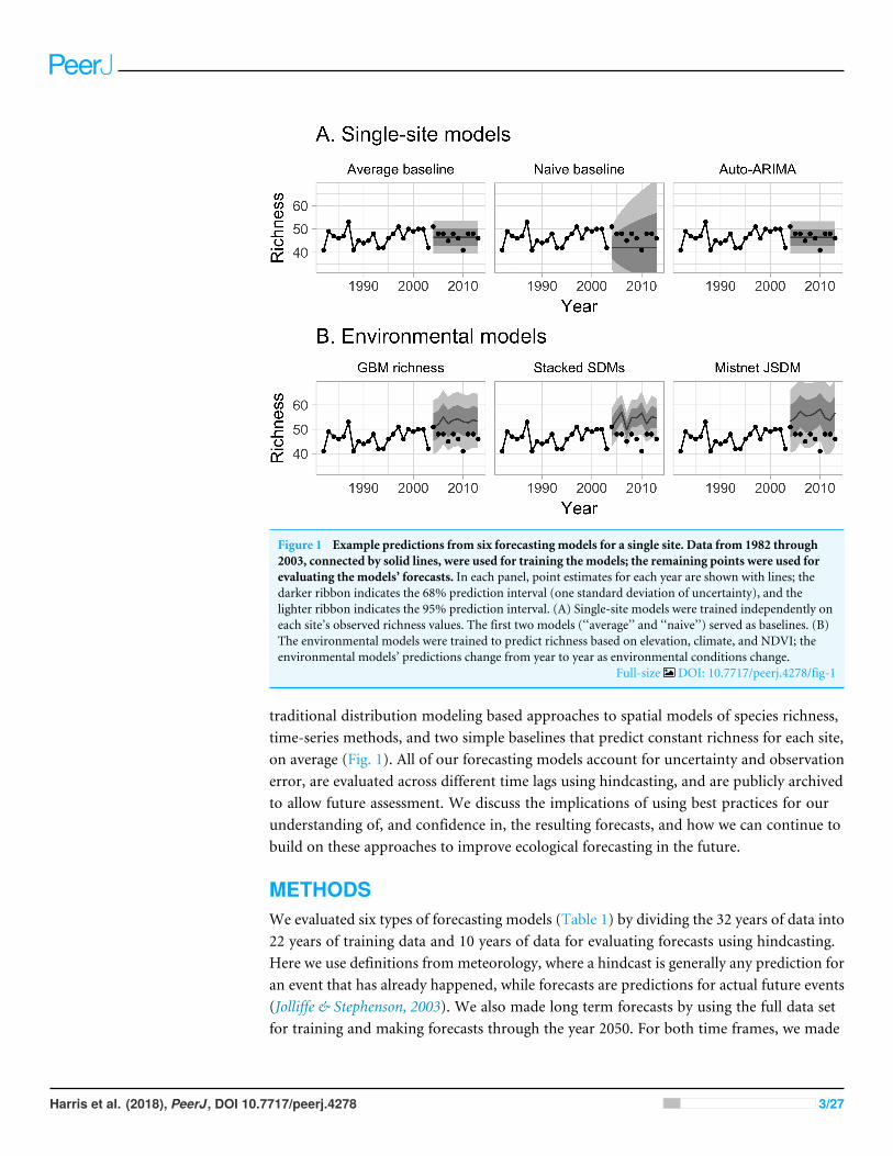
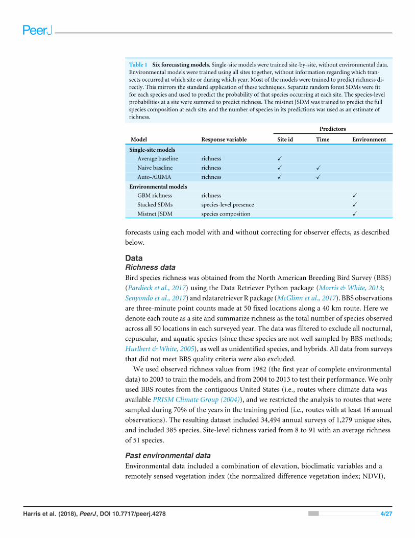
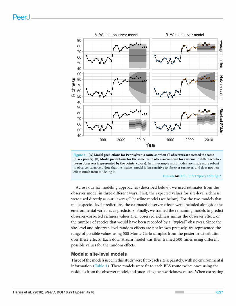
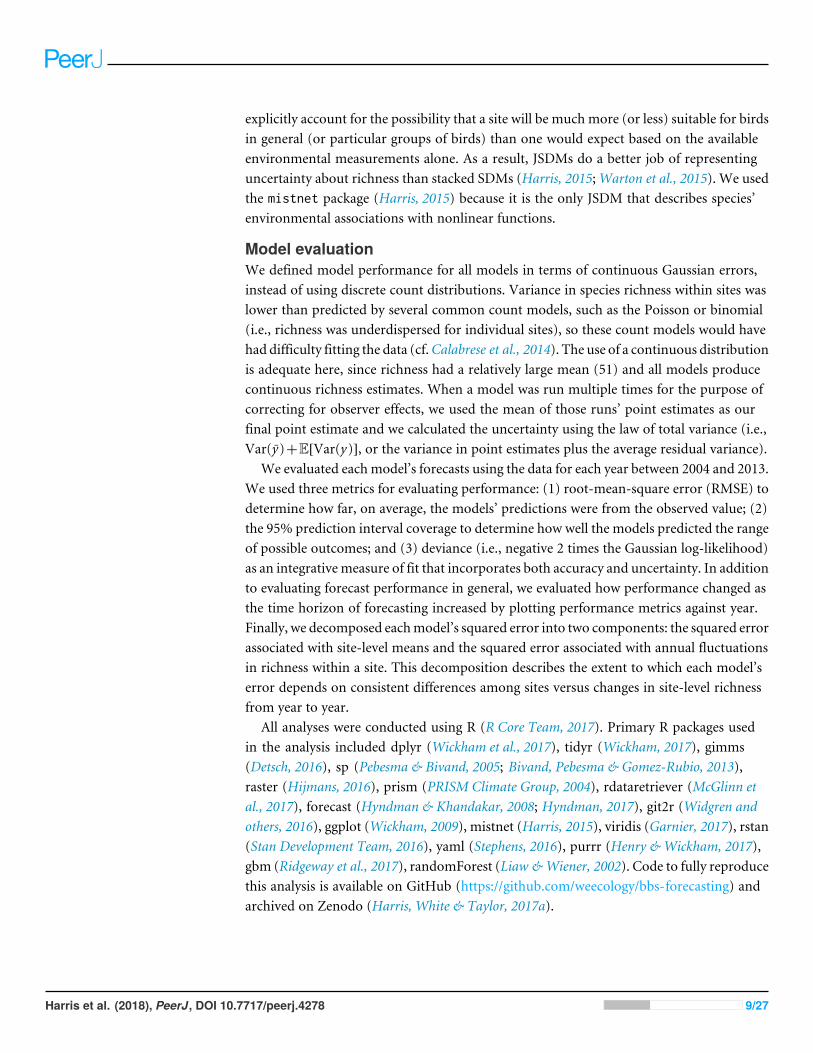
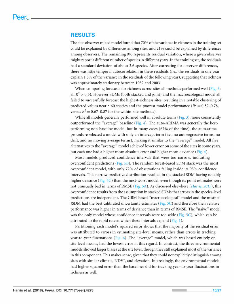
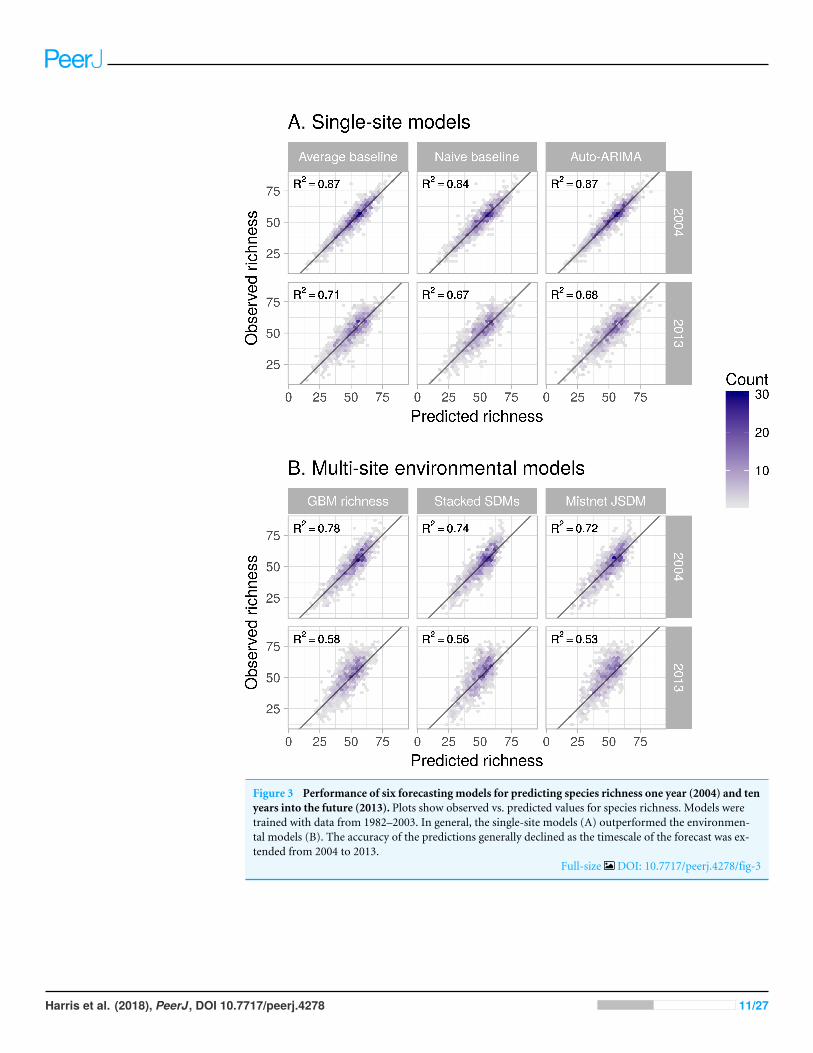
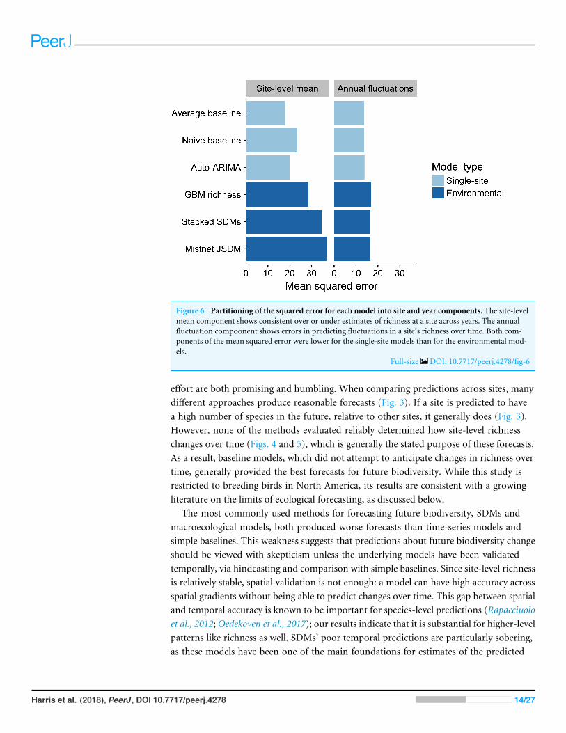
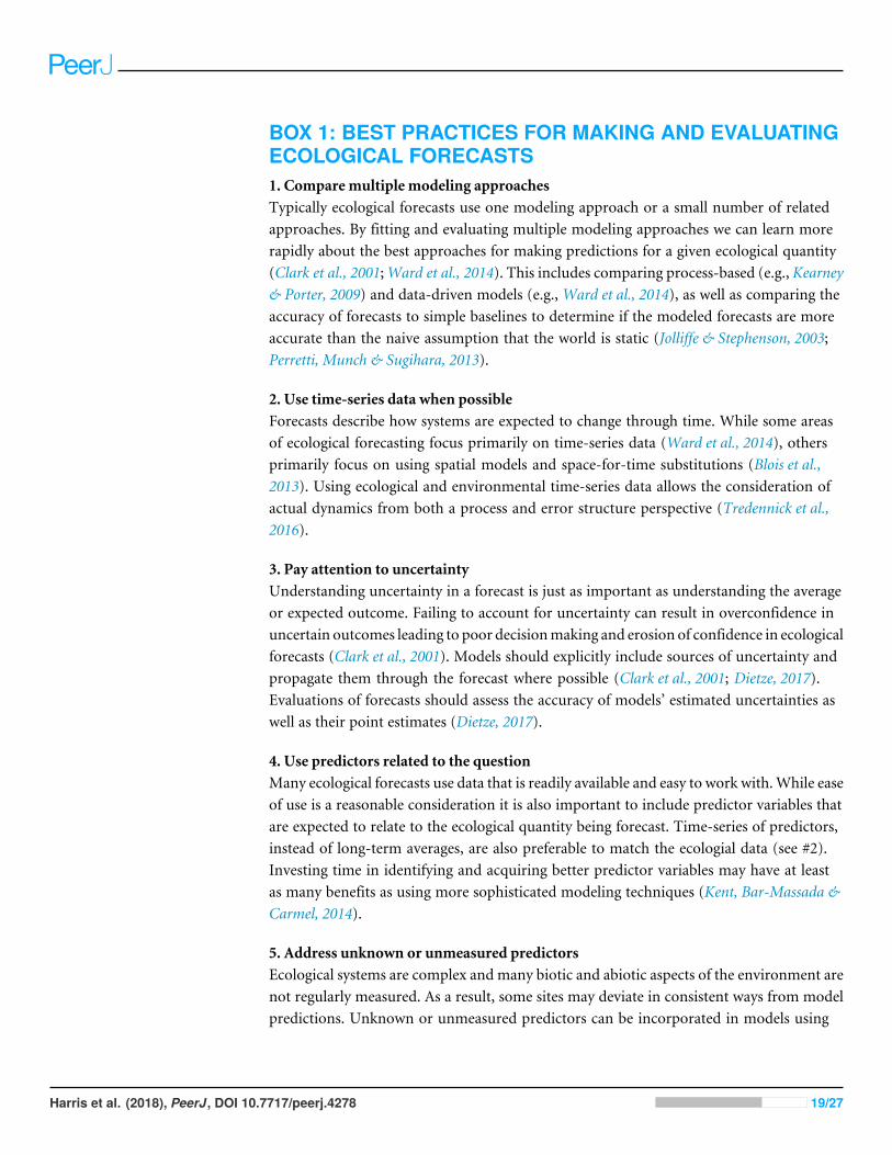
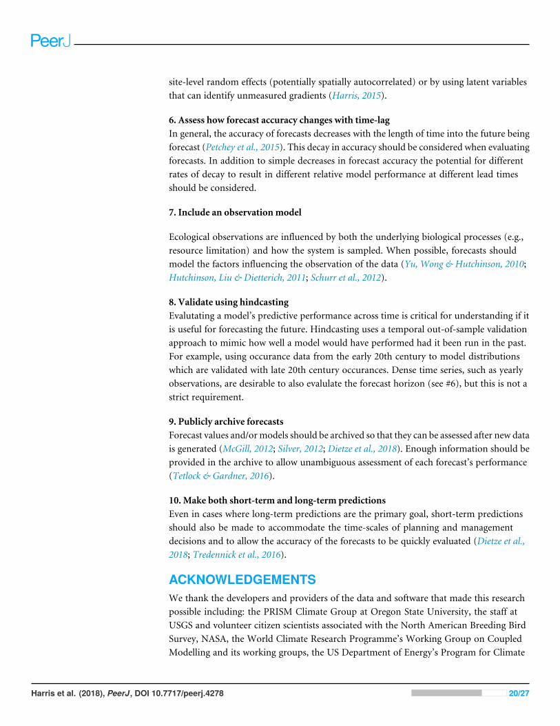