forecasting e-commerce key performance indicators · pdf fileforecasting e-commerce key...
TRANSCRIPT

Vrije Universiteit Amsterdam
Master Project Business Analytics
Forecasting E-commerceKey Performance Indicators
AuthorChi Chun Wan
November 13 2017
SupervisorMark Hoogendoorn
SupervisorVesa Muhonen
Contents
Preface 3
Abstract 4
1 Introduction 5
2 Background 721 Company Description 722 KPIs and Channels 7
221 KPIs 7222 Channels 8
23 Current Model 9
3 Literature Review 11
4 Data 1341 Google Analytics Data 1342 External Data 1543 Data pre-processing 1644 Data Analysis 16
5 Methods and Models 2151 Models 21
511 Ratio-based model 21512 ARIMA 23513 Random Forest 25514 Artificial Neural Networks 26
52 Multi-step Forecasting Strategies 3253 Evaluation 33
6 Experimental Setup 3561 Training and Testing 3562 Experiments 35
621 Experiment A 35622 Experiment B 36
63 Hyperparameters Optimization 37
1
7 Results 3971 Experiment A 39
711 Hyperparameters 39712 Model Performance 45713 Feature Importance 45714 Model Comparison 47
72 Experiment B 51721 Hyperparameters 51722 Model Performance 51723 Feature Importance 52
73 Summary 54
8 Discussion and Conclusion 55
References 57
Appendices 60
A Additional Results Data Analysis 60A1 The KPIs over monthly periods 60A2 The KPIs over weekdays 60
B Model Performance Experiment A 60B1 Visits 60B2 Transactions 60B3 Revenue 60B4 Media Spend 60
2
Preface
This internship report was written as the final part of the Masterrsquos pro-gram in Business Analytics at the Vrije Universiteit Amsterdam The goalof the Masterrsquos program in Business Analytics is to improve business perfor-mance by applying a combination of methods that draw from mathematicscomputer science and business management The internship was performedat FasterIntel During this internship I have focused on the forecast of e-commerce KPIs with the goal to improve this forecast The present thesisreports the results of my internship
I would like to thank FasterIntel for giving me the opportunity to completemy thesis I would also like to thank Eduard Belitser for being my secondreader Finally I want to give special thanks to my internal supervisor VesaMuhonen and VU supervisor Mark Hoogendoorn They have provided megreat guidance throughout the internship and useful feedback on the processand the report and I am very grateful for that
Chi Chun WanAmsterdam November 2017
3
Abstract
Key performance indicators or KPIs are important metrics usedin organizations to indicate their progress towards a defined businessgoal In the competitive e-commerce world it is important to obtainactionable insights as soon as possible Forecasting KPIs can helpthese e-commerce companies to have foresight to act on with theiractions to ensure business goals will be achieved The main objectiveof this thesis was to improve the prediction of KPIs using historicaldata Moreover the prediction will be implemented in the softwareplatform of FasterIntel and will be extended for multiple e-commercecompanies Therefore only data that is available in this softwareplatform and data that is generic enough to be available from allcompanies will be used These data are web tracking data from GoogleAnalytics and publicly available data
In this thesis we investigated eight different KPIs where four ofthem are predicted and the remaining four are derived from the pre-dictions The four predicted KPIs are the visits transactions revenueand media spend Moreover the forecast is based on 7 days ahead fore-cast Linear and non-linear models were implemented to produce theforecast The linear models are the Ratio-based model and ARIMAand the non-linear models are Random Forest Multi-Layer Perceptron(MLP) and Long Short-Term Memory (LSTM)
We conducted two experiments In the first experiment the pasthistory of the KPIs and time derived data from Google Analytics wereused and in the second experiment we extended this with externaldata and other Google Analytics features The results showed thatthis external data and these Google Analytics features did not improvethe forecast The best performance achieved for visits and transactionswas with Random Forest and for revenue and media spend with MLPThe improvement compared to the current model which is the simplelinear regression was 4175 1704 1702 and 5600 for visitstransactions revenue and media spend respectively However theforecast error was still large The reason is the limited historical dataavailable and the generic data More specific data might be useful toimprove the performance further
4
1 Introduction
With the evolution of the internet from a basic tool of communications intoan interactive market of products and services [1] many enterprises across theworld attempt to embrace e-commerce E-commerce also known as electroniccommerce consists of electronic business transactions to purchase and delivergoods and services E-commerce sales worldwide has grown from 137 trillionUS dollars to 186 trillion US dollar in 2016 and it is expected to grow to448 trillion US dollars in 2021 [2]
To aim for better performance in e-commerce measuring the key performanceindicators of e-commerce websites are important and cannot be overempha-sized Key performance indicators or KPIs are metrics that organizationstrack to measure their progress towards a defined business goal By trackingand measuring these indicators recommendation for operational improve-ment can be made based on actual data
There are many KPIs for an e-commerce website some of which are websitetraffic conversion rate sales and revenue In the field of KPIs a lot ofresearch has been done on finding factors that affect KPIs such as factorsthat will have impact on sales [3 4 5] However for forecasting KPIs mostresearch has only focused on sales forecast [6 7 8] For example Taylor[6] has focused on the forecast of daily supermarket sales to be applied ininventory control systems Lenort and Besta [7] have focused on the forecastof apparel sales to improve the effectiveness of the retailerrsquos sourcing strategyIn this research we will focus on the forecast of more KPIs besides sales Theforecast of KPIs will help e-commerce marketers to retrieve insights as soonas possible which is important in the competitive and crowded e-commerceworld They will have foresight to act on with their actions to ensure businessgoals will be achieved
The scope of this thesis is the forecast of KPIs for e-commerce brands which isoffered in the software product of FasterIntel This software product is a plugand play marketing platform for e-commerce brands and it currently displaysthe daily predictive performance of KPIs over different channel groups untilthe end of a week However the simple linear regression which is the currentmodel that is used for the prediction of these KPIs is not accurate enoughWhen e-commerce marketers rely on these predictions to make marketing
5
decisions these predictions should be as accurate as possible
In this research the goal is to improve the prediction of the KPIs usinghistorical data However since the prediction will be implemented in thesoftware product of FasterIntel and it must be scalable for multiple clientswe will encounter restrictions that makes it challenging One of these restric-tions is that only data that is available in the software product can be usedThis data consists of web-tracking data from Google Analytics Moreover ifweb-tracking data alone is insufficient to make accurate predictions then wehave to find external data that is still generic enough to be used for multipleclients This restriction leads to the following research question
With how much can the forecast of KPIs be improved compared to the currentmodel using only data that is generic enough to be available from all clients
The structure of the thesis consists of eight chapters The first chapter isthe current introduction Chapter 2 provides background information aboutFasterIntel the KPIs the channels and the current model used in the soft-ware product Next chapter 3 gives a literature review about the commonmodels used for time series forecasting and their application in forecastingKPIs Chapter 4 describes the data used followed by their pre-processingand analysis Chapter 5 describes the methods and models that have beenapplied for the forecast Chapter 6 describes the experimental setup andchapter 7 presents its results Lastly chapter 8 reports the discussion aboutthe results recommendation for future research and the conclusion
6
2 Background
21 Company Description
FasterIntel is a digital marketing company focusing on developing a plugand play marketing platform for e-commerce brands The features in theplatform are designed to save time and to boost revenue Features suchas decision insights that enable you to focus on making the right decisionsand conversion insights that provide insights and conversion rate trendsFasterIntel was separated from its parent company ConversionMob in 2017ConversionMob founded in 2011 is an online marketing agency that providesdigital and advertising consultancy services
22 KPIs and Channels
221 KPIs
FasterIntel displays the following eight most important e-commerce KPIs
1 Visits The total number of sessions where a session is a continuoususer interaction with your website The session expires after 30 minutesof inactivity and at midnight
2 Transactions The total number of completed purchases on the website
3 Revenue The total revenue from web e-commerce or in-app transac-tions
4 Media Spend1 The total amount paid for advertising within Google
5 Conversion Rate The proportion of visits that resulted in a transac-tion
Conversion Rate =Transactions
V isits
1Media Spend is not considered as a KPI but it is needed to compute ROAS and CPA
7
6 ROAS (Return On Ad Spend) The profit earned on the advertisingexpenses
ROAS =Revenue
Media Spendlowast 100
7 CPA (Cost Per Action) The average amount of advertising expendi-ture that is needed to generate an action
CPA =Media Spend
Transactions
8 Order Value The average value of a transaction
Order V alue =Revenue
Transactions
In this thesis we predict four out of these eight KPIs because the rest canbe derived These four KPIs are the visits transactions revenue and mediaspend
222 Channels
The KPIs can be filtered on different channel groups Channel grouping arerule-based groupings of the traffic sources It gives the ability to understandexactly how customers arrived at your website Moreover the performance ofeach of the traffic channels can be obtained This is useful as it gives insightabout which channel is performing best and which channel may require somemore work FasterIntel has defined the following 7 channels
1 Direct Going directly to the website
2 Organic Going via Google search
3 Paid Going via Google ads
4 Referral Going via other websitespages
5 Social Going via social media
6 E-mail Going via an e-mail such as newsletter
7 Other None of these 6 above
8
In this thesis we focus on the paid channel because during analysis we foundout that this channel gathers the most traffic Moreover this channel is af-fected by advertising which makes it harder to predict than the other chan-nels
23 Current Model
The simple linear regression is the current model that is used in the softwareproduct of FasterIntel to forecast the KPIs This linear regression modelcontains only one independent (explanatory) variable It is used to modelstatistical relationship between the independent (explanatory) variable andthe dependent (response) variable [9] The explanatory variables are vari-ables that have an effect on the response variable The response variableexpresses the observations of the data The model assumes a linear relation-ship between the response variable and the explanatory variable and findsthe best-fitting line (regression line) that describes this relationship Themodel is expressed as
Yi = a+ bXi + ei (21)
where the regression parameter a is the intercept and the regression param-eter b is the slope of the regression line Yi is the response variable at the ith
observation Xi is the explanatory variable at the ith observation and ei isthe residual at the ith observation The residual is the difference between theobserved response variable Yi and the predicted response variable Yi Thepredicted response variable Yi is given by
Yi = a+ bXi (22)
The best-fitting line is found using the least-square method This methodestimates the intercept a and the slope b such that the sum of squares error(SSE) is minimized The SSE is given by
SSE =nsum
i=1
(Yi minus Yi)2 (23)
9
Filling equation 22 into equation 23 and applying algebraically manipula-tion we will obtain the least squares estimates of the intercept a and theslope b
b =
nsumi=1
(Xi minus X)(Yi minus Y )
nsumi=1
(Xi minus X)2
a = Y minus bX
(24)
Here X is the mean of the explanatory variable and Y is the mean of theresponse variable
The current model always uses up to a maximum of 12 weeks of daily histor-ical data to fit the regression model The fitted regression model is then usedfor multi-step ahead prediction Daily predictions are made upon the end ofthe week (Sunday) Thus the number of days ahead forecast depends on thecurrent day and this maximum number will never exceed 7 days ahead Theregression model is refitted daily using new historical data This process willcontinue for each day and is visualized in Figure 21
Figure 21 The training and forecasting of the current model over the daysin each week Here the blue observations form the training sets and the redobservations are the forecast time steps
10
3 Literature Review
The daily prediction of the KPIs using their past observations is known astime series modeling A time series is a sequential set of data points measuredover successive times The aim in time series modeling is to collect and an-alyze the past observations of a time series to develop an appropriate modelthat describes the structure of the time series This model is then used toforecast future values for the time series Thus time series forecasting refersto the process of predicting future events based on past observations usingmathematical models A popular time series model is the AutoregressiveIntegrated Moving Average (ARIMA) [10] It is popular because of its flexi-bility and simplicity to represent different varieties of time series Howevera major limitation is the assumption that the time series is linear and fol-lows a particular known statistical distribution This approximation does nothold in many complex real-world problems Therefore non-linear models areproposed such as artificial neural networks (ANNs) [11] The major benefitof ANNs is their capability of flexible nonlinear modeling It is not neededto specify a particular model form because the model is adaptively formedbased on the features presented from the data
These models have been applied in forecasting sales and demand Cho [12]has applied exponential smoothing ARIMA and neural networks to predicttravel demand The analysis has shown that neural networks perform best forforecasting visitor arrivals especially in those series without obvious patternThe models were trained on the tourist arrival statistics in Hong Kong from1974 to 1998 Thiesing and Vornberger [13] have forecast the weekly demandon items in a supermarket using neural networks The neural network hasshown to outperform the naive method and the statistical method Theneural network was 17 more accurate than the statistical method and 32more accurate than the naive method The naive method is to use the lastknown value of the times series of sales as the forecast value for the nexttime step The statistical method is the moving average of sales of pastweeks Data that was used are the historical sales season and supermarketinformation such as the price and discount for every item holiday informationand opening hours of the store Alon et al [8] compared artificial neuralnetworks and traditional methods for forecasting aggregate retail sales Theresults have shown that ANN performed the best followed by ARIMA and
11
Winters exponential smoothing Moreover ANN was able to capture thedynamic nonlinear trend and seasonal patterns and their interactions
Features that are relevant in forecasting sales are information about the prod-ucts that are sold However these features cannot be used in this researchbecause they are not generic enough Reijden and Koppius [14] have shownthat measures of online product buzz variables increase the accuracy of salesforecasting with 28 These online product buzz refers to online expressionof interest in a product such as online product review blog post and searchtrends Moreover they found that a random forest technique is very suitableto incorporate these online product buzz variables Ferreira et al [15] foundthat the features with largest variable importance are the discount pricepopularity and brand of the product They used machine learning tech-niques to forecast demand of products for an online retailer and found thatregression trees with bagging outperformed other regression model Meulsteeand Pechenizkiy [16] improved the food sales prediction for each product byconstructing new groups of predictive features from publicly available dataabout the weather and holidays and data from related products MoreoverMurray et al [17] provided empirical evidence to explain how the weatheraffects consumer spending They found that when exposure to sunlight in-creases negative affect decreases and consumer spending tends to increase
12
4 Data
This section describes the data and its pre-processing Moreover data anal-ysis will be performed
41 Google Analytics Data
Google Analytics (GA) is a web analytics service offered by Google thattracks and reports website traffic [18] It sets a first party cookie as trackingcode on each visitorrsquos device Thus users are just cookies and not individualsFor this research we used GA data from one of the clients of FasterIntelEvery report in GA is made up of dimensions and metrics Dimensions areattributes of your data and metrics are quantitative measurements In ourdataset the dimensions are the date source and medium which are combinedwith different metrics The dataset along with its description is shown inTable 41
13
Data Description
DimensionsDate The date of the active date rangeSource The place users were before seeing your contentMedium Description of how users arrived at your content
MetricsTimeYear The year of the dateMonth The month of the dateWeek The week of the dateWeekday The weekday of the dateSeason The season of the date according to the four-season calendar reckon-
ingHoliday Variable indicating whether the date is a holiday in the NetherlandsKPIsSessions The total number of sessions (visits)Transactions The total number of completed purchases on the websiteRevenue The total revenue from web e-commerce or in-app transactionsAd Cost The total amount paid for advertising (media spend)AdvertisingImpression The number of times your ad is shown on a search result page or
other site on the Google networkAd Clicks The number of times someone clicks on your adActive campaigns The number of active campaignsSessionsBounce Rate The percentage of all sessions on your site in which users viewed only
a single page and triggered only a single request to the Analyticsserver
Percentage NewSessions
The percentage of sessions by users who had never visited the prop-erty before
Average SessionDuration
The average duration (in seconds) of usersrsquo sessions
UsersUsers The total number of users for the requested time periodNew Users The number of sessions marked as a userrsquos first sessionsSite SpeedAverage PageLoad Time
The average time (in seconds) pages from the sample set take to loadfrom initiation of the pageview to load completion in the browser
Average Redirec-tion Time
The average time (in seconds) spent in redirects before fetching thispage
Table 41 Google Analytics data and its description per day
The dataset consists of metrics for each day from 1 July 2014 to 31 May2017 for each corresponding source and medium The metrics can be dividedinto categories The time category consists of data that are derived from thedate The rest of the categories consists of data that are self explanatory
42 External Data
Besides the GA data external data is used This external data consistsof the weather inflation and the unemployment in the Netherlands Theweather data is obtained from Koninklijk Nederlands Meteorologisch Insti-tuut (KNMI) [19] and the others are obtained from Centraal Bureau voorde Statistiek (CBS) [20] The external data along with its description canbe found in Table 42 This external data could have an effect on the KPIsFor instance weather has an effect on consumer spending as shown in theliterature review
Data Description
WeatherAverage Temperature The average daily temperature (in 01 degree Celsius)Minimum Temperature The daily minimum temperature (in 01 degree Celsius)Maximum Temperature The daily maximum temperature (in 01 degree Celsius)Rainfall Amount The daily amount of rainfall (in 01 mm)Rainfall Duration The daily rainfall duration (in 01 hour)Sunshine Duration The daily sunshine duration (in 01 hours) calculated
from the global radiationInflationInflation Rate The monthly inflation rate (consumer price index) in
percentageUnemploymentUnemployment The percentage of unemployed (monthly)
Table 42 External data and their description
15
43 Data pre-processing
44 Data Analysis
In order to obtain insights from the data several analyses have been per-formed
From these analyses an overview of the time effect on the KPIs is obtained
The next analysis is the correlation between the KPI values and their ownlags This is analyzed using the autocorrelation function (ACF) and partialautocorrelation function (PACF) Both functions measure the correlation be-tween the current observation and an observation k time step ago but thepartial autocorrelation also takes into account the observations at intermedi-ate lags (ie at lags lt k) [21] They can be used to determine the magnitudeof the past values related to future values [10]
The ACF and PACF plots of the KPIs on the paid channel are shown inFigures 41 and 42
16
(a) Visits (b) Media Spend
(c) Transactions (d) Revenue
Figure 41 ACF plot of the KPIs on the paid channel The blue dashed linesindicate the point of statistical significance
17
(a) Visits (b) Media Spend
(c) Transactions (d) Revenue
Figure 42 PACF plot of the KPIs on the paid channel The blue dashedlines indicate the point of statistical significance
We observe that the ACF plot shows a slight peak at every 7th lag for allKPIs This indicates a weekly pattern The PACF plot shows a significantspike at lag 1 for all KPIs This indicates that the KPI value of previousday is very strong correlated with the value of current day For visits andmedia spend the lags 1 to 7 is significantly positive correlated Moreoverlag 8 is negative correlated and lags beyond 8 become less significant Fortransactions and revenue we observe significance until lag 7 followed by aspike at lag 14 that is caused by the weekly pattern
18
The final analysis is the exploration of the statistical relationship between theKPIs and the other metrics in the data The Pearson correlation between thedifferent variables in the data is computed Since we use past observations topredict the KPIs the correlation is between the current day KPIs value andthe metrics value of previous day except for weather inflation and unemploy-ment The values for weather are at the same day because weather forecastcan be derived from other resources This forecast can then be used as pre-dictor for the KPIs The value for inflation and unemployment is from theprevious month because daily observations are not available Even thoughthis is the case it can still help in daily forecast as inflation and unemploy-ment usually have a long term effect The correlation matrix for the paidchannel is shown in a correlogram in Figure 43
Figure 43 Pearson correlation matrix of the data on the paid channel
19
We observe correlations between KPIs themselves Visits (gasessions) ispositive correlated with media spend (gaadCost) which indicates that anincrease in media spend of the previous day results in an increase in next dayvisits Transactions is strong positive correlated with revenue (gatransactionRevenue)which is obvious The current day visits is strong correlated with previousday users and new users This can be explained by the fact that every singleuser generates at least one session Moreover a positive correlation is ob-served between visits and impressions and adClicks which shows the positiverelation between advertising and visits
For media spend we observe a positive correlation with impressions adclicksand number of active campaigns which is natural
With the obtained insights from the data analysis we have a good interpre-tation about which data can be used as features in the models This will befurther described in the experiments in section 62
20
5 Methods and Models
This section describes the models that are used for the forecast the multi-step forecasting method and the evaluation method
51 Models
511 Ratio-based model
The Ratio-based model is used as a benchmark model This model takes thehistorical data of a certain number of weeks before and computes the changein ratios over the same day for every week Next these ratios are averagedinto a single ratio and this single ratio is used as predictor for the next timestep
If we define Xt as the KPI at time step t and we take k weeks as historicaldata then the ratio change for Xt is given by
Ratiot =1
k
ksumi=1
Xt+1minus7i minusXtminus7i
Xtminus7i(51)
However problem occurs when the historical KPIs are zero ie Xtminus7i = 0for i = 1 k This will result in a division of zero which is not possibleTherefore in this case we take the difference of the KPIs instead of the ratio
Differencet =1
k
ksumi=1
Xt+1minus7i minusXtminus7i (52)
Moreover the difference forecast will be applied when Xt is zero as the ratioforecast will always result in a zero Thus the forecast on Xt+1 is given by
Xt+1 =
Xt lowast (1 + Ratiot) if Xt gt 0 or Ratiot is definedXt + Differencet if Xt = 0 or Ratiot is undefined
(53)
21
This equation expresses the single-step forecast The mathematical expres-sion for the recursive multi-step forecast is then
Xt+n =
nminus1prodi=0
(1 + Ratiot+i) lowastXt if Xt gt 0 or Ratiot+i is defined
nminus1sumi=0
Differencet+i +Xt if Xt = 0 or Ratiot+i is undefined
(54)
Notice that the ratio and the difference are always taken on the next timestep ie the ratio and difference between Xt and Xt+1 However we can alsotake the ratio and difference between multiple time steps ie between Xt andXt+n This will avoid the recursive strategy that usually has accumulatederror The ratio and the difference are then expressed as
Ratiot+n =1
k
ksumi=1
Xt+nminus7i minusXtminus7i
Xtminus7i
Differencet+n =1
k
ksumi=1
Xt+nminus7i minusXtminus7i
(55)
Next the non-recursive multi-step ahead forecast is given by
Xt+n =
Xt lowast (1 + Ratiot+n) if Xt gt 0 or Ratiot+n is definedXt + Differencet+n if Xt = 0 or Ratiot+n is undefined
(56)
The Ratio-based model for both the recursive and non-recursive multi-stepahead is illustrated in Figure 51
22
(a) Recursive forecast
(b) Non-recursive forecast
Figure 51 The Ratio-based model recursive and non-recursive forecastusing one week historical data The blue observations are the historicalobservations and the red observations are the forecast time steps
The advantage of this model is its simplicity and flexibility The model canbe easily implemented for all the KPIs and it is able to produce a forecasteven when little data is available The disadvantage is the reliability of themodel as large variation in KPIs over the weeks can easily result in inaccurateforecast
512 ARIMA
The ARIMA model is a stochastic time series model that combines threeprocesses the Autoregressive process (AR) the strip off of the integrated (I)time series by differencing and the Moving Averages (MA) [10] In an ARprocess the future value of a variable is assumed to be a linear combinationof p past observations plus a random error and a constant In a MA processthe past observations are the q past errors instead of the past observationsThus it is a linear combination of q past errors plus a random error and themean of the series These two processes can be combined together to forma more effective time series model This model is known as ARMA(pq) [22]and is given by
23
Xt = α1Xtminus1 + + αpXtminusp + εt + β1εtminus1 + + βqεtminusq (57)
where Xt is the observation at time t and εt is the random error at time tThis equation can be written implicitly as
(1minus
psumk=1
αkLk)Xt =
(1 +
qsumk=1
βkLk)εt (58)
where p and q are the order of the autoregressive and moving average partsof the model respectively and L is the lag operator
However ARMA can only be used for stationary time series ie the meanand variance of the time series do not depend upon time This is not the casein many time series such as in economic time series that contain trends andseasonal patterns Therefore the integrated term is introduced to include thecases of non-stationarity by applying differencing The difference operatortakes a differencing of order d and it is expressed as follows
∆dXt = (1minus L)dXt (59)
where Xt is the data point at time t L is the lag operator and d is the orderThus the three processes AR(p) I(d) and MA(q) are combined interactedand recomposed into the ARIMA(p d q) model
The general method to identify the order p in an AR process and q in aMA process is to use the autocorrelation function (ACF) and the partialautocorrelation function (PACF) [21] For a pure AR(p) process the PACFcuts down to zero after lag p For a pure MA(q) process the ACF cuts downto zero after lag q For ARMA(p q) and ARIMA(p d q) processes it is morecomplicated to estimate the parameters A method to do this is to performa grid search over these parameters using an evaluation metric for modelselection
24
513 Random Forest
Random Forest is a machine learning model for classification and regression[23] and it is illustrated in Figure 52
Figure 52 Random Forest [24]
Random Forest is an ensemble learning method that combines a group ofweak learners to form a more powerful model These weak learners are deci-sion trees and they can either be used for classification or regression In ourcase the focus is on regression
A decision tree is made up of decisions nodes terminal nodes (leaves) andbranches These branches represent the possible paths from one node toanother Decision trees are recursive partitioning algorithm that split thedataset in smaller subsets using a top-down greedy approach It starts atthe root node (top decision node) where a certain feature variable is usedto split the data into subsets Because the dataset can be split in numerousways the feature variable and its split point that yields the largest reductionin the residuals sum of squares (RSS) is chosen
Nsumn=1
sumiisinRn
(yi minus yn)2 (510)
where yi is the training observation i and yn is the mean of the responsevalues for the training observation that fall into the subset n
25
Next the decision tree recursively splits the dataset from the root nodeonwards at each decision node until the terminal nodes These terminalnodes are the endpoints of the decision tree and represent the final result ofa combination of decisions and events They are reached when all recordsafter the split belong to the same target variable or until a stopping criterionis met
In Random Forest a large number of these decision trees are constructed andeach tree makes a random selection of independent variables This results invariance in predictions between various decision trees which reduce overfittingand variance Then the prediction is produced by taking the mean predictionof the individual trees
Besides the number of trees in the forest it has other parameters that canbe varied such as the maximum depth of the tree the minimum number ofsamples required to split a decision node the minimum number of samplesrequired to be at a leaf node and the number of features to consider whenlooking for the best split
514 Artificial Neural Networks
ANNs are inspired by biological systems and the human brain and they haveshown powerful pattern classification and recognition capabilities [11] ANNslearn from experience by recognizing patterns in the input data Next theymake predictions based on their prior knowledge ANNs are applied in manydifferent fields of industry business and science [25] There are differenttypes of ANNs we have applied the feed-forward neural network (FNN) andthe recurrent neural network (RNN) [26 27] The FNN is the Multi-LayerPerceptron and the RNN is the Long Short-Term Memory
5141 Multi-Layer Perceptron
The Multi-Layer Perceptron (MLP) is a class of FNN Figure 53 illustratesthe architecture of a MLP
26
Figure 53 Architecture of a MLP with 3 layers (input hidden and output)with 4 input neurons 5 hidden neurons and 1 output neuron [28] Noticethat MLP can have multiple hidden layers
The network consists of processing elements also known as neurons that areorganized in layers Every neuron in a layer is connected with all the neuronsin the previous layers by acyclic links each with an associated weight Theseweights encode the knowledge of a network The neurons in the layers areused for transformation from input to output The output of each neuron yin the hidden layer(s) and output layer is a (non) linear function over the dotproduct of the weights of the connections with the outputs of the neurons inthe previous layer
y = φ
(sumi
ωixi + b
)(511)
Here xi are the inputs of the neuron ωi are the weights of the neuron and bis the bias φ is the activation function that determines the activation levelof the neuron
During training of the network the weights are modified such that the dif-ference between the network output and the actual output are minimized
27
Thus the estimation of the weights are based on the minimization of thecost function In our model this cost function is the mean squared errorIn order for the network to know how to adjust the weights it uses learningalgorithms The traditional learning algorithm is backpropagation [29] andit works as follows
1 Compute the feed-forward signals from the input to the output
2 Compute the error E of each neuron of the output layer using the costfunction
3 Backpropagate the error by the gradients of the associated activationfunctions and weighting it by the weights in previous layers
4 Compute the gradients for the set of parameters based on the feed-forward signals and the backpropagated error
5 Update the parameters using the computed gradients
∆ωij = αδjyi where (512)
δj =
φprime(vj)(tj minus yj) if j is an output nodeφprime(vj)
sumk of next layer δkωjk if j is an hidden node
Here ωij is the weight between node i and node j α is the learningrate yj is the output of node j vj is the activation of node j and tj isthe target output of node j
Even though backpropagation is used to solve many practical problems itshows problems such as slow convergence and getting stuck at local minima[29] Therefore other learning algorithms have been developed to improvethe performance of the backpropagation algorithm One of these learningalgorithms is the Adaptive Moment Estimation (Adam) [30] Adam is astochastic gradient descent algorithm based on estimation of first and secondorder moments of the gradients The algorithm works as follows
1 Compute the gradient using the current parameters
2 Update biased first order and second order moments estimate
mt = β1mtminus1 + (1minus β1)gtvt = β2vtminus1 + (1minus β2)g2t
(513)
28
Here mt is first order moment at time step t vt is the second ordermoment at time step t gt is the gradient at time step t and g2t indicatesthe element-wise square of gt β1 and β2 are the exponential decay ratesbetween 0 and 1
3 Compute the bias-corrected first and second order moments
mt =mt
1minus βt1
vt =vt
1minus βt2
(514)
4 Compute weight update and update parameters
θt = θtminus1 minus αmt
(radicvt + ε)
(515)
Here θt is the parameter vector at time step t and α is the learningrate
Adam computes adaptive learning rates for each parameter [31] that speedsup the learning phase This leads to faster convergence Furthermore littlemanual tuning of hyperparameters are required because they have intuitiveinterpretation All these advantages are beneficial for all the models thatneed to be constructed Therefore Adam is used as learning algorithm
5142 Long Short-Term Memory
In FNNs information is only propagated in one direction This is in contrastto recurrent neural networks (RNNs) where information is propagated in bi-directions using feedback loops These feedback loops transfer internal andoutput signals back to the input level which allows information to persistThus a RNN has an internal memory that captures information about whathas been calculated so far This becomes clear if we unfold the RNN throughtime as shown in Figure 54
29
Figure 54 A RNN unfolded in time [32] Here U V W represent the set ofweights xt is the input at time step t st is the hidden state at time step tand ot is the output at time step t
Therefore RNNs can model temporal dependencies of unspecified durationbetween the inputs and the associated desired outputs [33] Because of thisRNNs are suitable for time series predictions However when the gap be-tween the relevant information and the prediction becomes larger regularRNNs become unable to learn to connect the information because of thevanishing gradients (ie the gradient gets so small that learning either be-comes very slow or stops) The problem of vanishing gradients can be avoidedusing Long Short-Term Memory (LSTM)
LSTM is a specific RNN that is capable of learning long-term dependenciesand it was introduced by Hochreiter and Schmidhuber [34] The networktakes three inputs The input Xt of the current time step t the output fromthe previous LSTM unit htminus1 and the memory of the previous unit Ctminus1
The LSTM unit contains special units called memory blocks in the recurrenthidden layer An individual memory block is shown in Figure 55 Eachmemory block contains memory cells and three gated cells that is shared byall the memory cells These three gates are the forget input and output gateand control the information flow to the cells The forget gate decides whatinformation will be removed in the memory The input gate decides whatinformation will be updated The output gate defines what information insidethe cells will be exposed to the external network These gates are controlledby a simple one layer neural network using the sigmoid activation functionThus the network outputs a value between 0 and 1 where 0 represents closed
30
gates and 1 represents open gates
Figure 55 A single LSTM memory block [35]
The forget and input gate use the three LSTM network inputs Xt htminus1 andCtminus1 and a bias vector as input The output gate uses the htminus1 Xt the newmemory Ct and a bias vector as input Thus the forget gate ft input gateit and output gate ot of the current time step t is given by the followingequations
ft = σ(bf +WxfXt +Whfhtminus1 +WcfCtminus1)
it = σ(bi +WxiXt +Whihtminus1 +WciCtminus1)
ot = σ(bo +WxoXt +Whohtminus1 +WcoCt)
(516)
Here σ is the sigmoid function b is the bias vector and W represents the setof weights
The new memory Ct is also generated by a simple neural network but it usesthe hyperbolic tangent as activation function instead of the sigmoid functionThe new memory Ct is then generated by element-wise multiplication of theinput gate it and by adding the old memory Ctminus1
31
Ct = ftCtminus1 + it tanh(bc +WxcXt +Whchtminus1) (517)
Here tanh is the hyperbolic tangent function b is the bias vector and Wrepresents the set of weights
The output ht for the LSTM unit is then generated using the new memoryCt that is controlled by the output gate ot
ht = ot tanh(Ct) (518)
Again the weights in the network need to be learned The learning algorithmAdam is used for this purpose because it can handle the complex training dy-namics of RNNs better than plain gradient descent [30] Moreover since thenetwork uses the hyperbolic tangent function as activation function whichis bounded between -1 and 1 the data is normalized between -1 and 1
52 Multi-step Forecasting Strategies
Since FasterIntel always shows predictions of the KPIs up to Sunday (endof the week) for each week it means that it requires a maximum of 7 daysahead forecast Therefore we decided to forecast the KPIs always 7 timesteps ahead on each day Predicting multiple time steps into the future isalso known as multi-step time series forecasting Different strategies are usedfor multi-step time series forecasting [36] The most common strategies arethe direct multi-step forecast and the recursive multi-step forecast The di-rect multi-step forecast uses a separate model for each forecast time stepwhile the recursive multi-step forecast uses a one-step model multiple timesIt takes the prediction for the prior time step as an input for making a pre-diction on the following time step A disadvantage of the recursive strategyis the accumulation of the prediction errors as the forecast horizon increaseswhile this does not hold in the direct strategy However this does not meanthat the direct strategy is always better than the recursive strategy It alldepends on the model specification Another disadvantage of the recursivestrategy are the unknown values for other time series when they are usedas predictors This means that each time series need to be predicted Thedisadvantage of the direct strategy is that it involves a heavier computationalload than the recursive strategy Moreover since the direct strategy forecasts
32
each time step in isolation of the other time steps it can produce completelyunrelated forecasts over the whole forecast horizon This can lead to un-realistic discontinuities whereas time series have some aspect of continuousbehavior in reality [37] Therefore the recursive strategy is applied in thisresearch
53 Evaluation
The performance of the models is evaluated using the time series cross vali-dation This process is illustrated in Figure 56
Figure 56 The series of training and test sets in time series cross validationThe blue observations form the training sets and the red observations formthe test sets [38]
This validation has a series of training and test sets Each of the test setsconsists of n observations that corresponds with the n time step ahead fore-cast The corresponding training set consists of features that occurred priorto the first observation of the test set This mimics the real-world scenariowhere new observations become available for each time step t Next thisvalidation method walks each series of the test sets one at a time and makesn predictions for each time step
Next the real observations and the predictions for each time step are com-pared with each other using an error measurement The error measurementthat is used is the Root Mean Squared Error (RMSE) and it is given by
33
RMSE =
radicradicradicradic 1
m
msumi=1
(yi minus yi)2 (519)
Here yi is the predicted value for observation i yi is the actual value forobservation i and m is the total number of observations
The RMSE penalizes extreme errors as it is much affected by large individualerrors Thus we obtain n RMSE values where each of these values representsthe error for a single time step t t+ 1 t+ n
34
6 Experimental Setup
This section describes the training and testing of the models the two exper-iments that are conducted and the optimization of the model hyperparame-ters
61 Training and Testing
Since the KPIs have seasonality within a year as shown in the analysis insection 44 it is important that the models are evaluated on at least one yeartest data to capture their overall performance Therefore we chose the last365 days of the dataset as test set starting from 25 May 2016 Notice thatit does not start from 31 May 2016 because observations after 31 May 2017are not available in the dataset when performing 7 days ahead forecast
The models are retrained after each 30 series This corresponds with retrain-ing the model every month The decision to not retrain the models every dayis because retraining on one new observation in the training set will hardlymake any difference in terms of performance
62 Experiments
In this research two experiments have been conducted These experimentsare categorized into experiment A and experiment B
621 Experiment A
In experiment A the data used for each KPI forecast are the correspondinghistorical KPI data along with time related data The time related data arethe month week weekday season and holiday The choice of performing thisexperiment is because the current forecast model only uses the correspondinghistorical KPI data Thus it is interesting for FasterIntel to know about thepredictive performance of each model using only this data The time relateddata is used to capture temporal information from the time series for RandomForest and MLP because they are non-temporal models This is in contrast
35
with ARIMA and LSTM which are temporal models that should be able tocatch temporal information automatically from the time series Thus theinput data for ARIMA and LSTM are only the lagged values of the KPIunder investigation whereas Random Forest and MLP added additional timerelated data and the weekly moving average of the KPI as input to spot theweekly trend
The total number of lags to consider in each model are determined in differentways depending on the model In ARIMA the number of lags is the orderp in the AR part and q in the MA part This order is determined using agrid search method on the validation set that will be described in section63 In LSTM a lag of one is used because information of the lags are passedthrough each recurrent state to the next state In Random Forest and MLPthe number of lags are based on the PACF analysis in section 44 For visitsand media spend the first 8 lags are used and for transactions and revenuethe first 7 lags and the 14th lag are used
Random Forest and ANNs are run for multiple times and the average perfor-mance was taken as final performance for the models This is because thesemodels are stochastic and therefore they return different results on differentruns of the same algorithm on the same data
622 Experiment B
In experiment B all the data are used in the KPIs forecast With this ex-periment we are able to show the difference in performance compared toexperiment A when more data is added This could be interesting for Fas-terIntel as they can set up new businesses with their clients eg offeringbetter KPIs predictive performance for only premium clients However weonly forecast one step ahead instead of multi-step ahead because it becomescomputationally too intensive when additional time series features are addedThe reason is that the recursive strategy requires predictions for every addi-tional time series feature and developing models to do so was out of scopein this thesis Notice that ARIMA is excluded in this experiment as it is aunivariate time series model
In order to ensure that the difference in performance is caused by addingadditional features the same features in experiment A plus the additional
36
features are used These additional features are chosen based on the analysisof the Pearson correlation matrix as shown in Figure 43 The additionalfeatures for the KPIs are shown in Table 61
KPI Additional Features
Visits rdquoad costrdquo rdquousersrdquo rdquonew usersrdquo rdquoimpressionrdquordquoinflationrdquo rdquounemploymentrdquo
Transactions rdquoad costrdquo rdquousersrdquo rdquonew usersrdquo rdquoimpressionrdquordquoaverage temperaturerdquo rdquomaximum temperaturerdquordquoinflationrdquo rdquounemploymentrdquo
Revenue rdquoad costrdquo rdquousersrdquo rdquonew usersrdquo rdquoimpressionrdquordquoaverage temperaturerdquo rdquomaximum temperaturerdquordquoinflationrdquo rdquounemploymentrdquo
Media Spend rdquoimpressionrdquo rdquocampaignsrdquo rdquoad clicksrdquo
Table 61 KPI and its additional features
Again the number of lags for each feature had to be determined in the inputdata as in experiment A Zero lag is chosen for the temperature data as yourcurrent behaviour can be influenced by the current weather condition Alag of one is chosen for the other additional features because it is the mostrepresentative for the current time step Moreover the moving average of 7days for all Google Analytics features and the weather is included which giveinformation about the weekly trend of each time series feature
63 Hyperparameters Optimization
ARIMA Random Forest MLP and LSTM all have hyperparameters thatneed to be optimized to achieve good performance The hyperparametersin ARIMA are the auto regressive order p the integration order d and themoving average order q For Random Forest MLP and LSTM not all hyper-parameters are considered The ones that are considered in Random Forestare the number of trees in the forest the number of features to consider whenlooking for the best split and the minimum sample leaf size The hyperpa-rameters that are considered in MLP are the number of hidden layers andneurons in each layer and the activation functions The hyperparameters
37
that are considered in LSTM are the number of hidden layers and LSTMunits in each layer
All the combinations of the hyperparameters were tested on the validationset This validation set is a separation of the first training set in the timeseries cross validation and contains one month of data starting from 25 April2016 to 24 May 2016 Thus the models were trained on the data before 25April 2016 Next each model was trained again on the whole first trainingset using the optimal hyperparameters and evaluated using time series crossvalidation as described in section 53
The hyperparameter optimization for ARIMA was performed using a gridsearch method This method tries every hyperparameter setting over a spec-ified range of values The search range for the autoregressive order p andmoving average order q was set based on the PACF and ACF analysis insection 44 respectively For the autoregressive order p it was set from 0 to8 for visits and media spend and from 0 to 14 for transactions and revenueFor the moving average order q it was set from 0 to 7 for all the KPIs Thesearch range for the integration order d was set from 0 to 1 The choice fora maximum of first order differencing is because second order differencing israrely needed to achieve stationarity [10]
In Random Forest the optimal number of trees was determined to be inthe range from 10 to 400 and the optimal minimum sample leaf size wasdetermined to be in the range from 1 to 50
In MLP the optimal hidden neurons in each hidden layer was determined inthe range 10 to 100 The number of hidden layers was set to a maximum oftwo layers The rectified linear unit (ReLU) activation function was used inthe hidden layers because it was found to be the most efficient when appliedto the forecasting of non-stationary and noisy time series Next the linearactivation function was used in the output layer to output the forecast valueof the time series
In LSTM the number of hidden layers was set to one and the number ofLSTM units was determined in the range 10 to 40 The exponential decayrates β1 and β2 were set to default values of 09 and 0999 respectively Thesedefault values are proposed in the original paper [34]
38
7 Results
In this section the results of the two experiments are presented First section71 presents the results for experiment A and it contains results with regardsto model hyperparameters model performance model comparison and fea-ture importance Next section 72 presents the results for experiment Band it contains results with regards to model hyperparameters model per-formance and feature importance Finally section 73 summarizes the resultsof both experiments
71 Experiment A
711 Hyperparameters
The results for the hyperparameters for ARIMA Random Forest and MLPare shown below
39
ARIMA
Figure 71 ARIMA Order(p d q)2
Figure 71 shows the RMSE for different combinations of order(p d q) Weobserve many fluctuations in errors for the different combinations The op-timal order achieved for visits transactions revenue and media spend is(605) (202) (402) and (706) respectively
2The order(p d q) starts at (000) and is first incremented for q next for d and as lastfor p
40
Random Forest
Figure 72 Random Forest Number Of Trees
Figure 72 shows the RMSE for different number of trees We observe thatthe optimal number of trees for visits is 270 as increasing the number oftrees will not significantly decrease the RMSE anymore For transactionsthe RMSE becomes stable after 120 trees The number of trees that is chosenfor revenue and media spend is 300 and 370 respectively It is not necessaryto increase the number of trees further as the performance stays roughly thesame while the computational time will increase
The optimal maximum number of features to look for the best split wasfound to be the square root of the number of input features The optimalminimum sample leaf size in experiment A was 7 2 3 and 2 for visitstransactions revenue and media spend respectively In experiment B theoptimal minimum sample leaf size was 4 1 4 and 1 for visits transactionsrevenue and media spend respectively
41
MLP
Figure 73 MLP number of hidden layers and hidden neurons
Figure 73 shows the RMSE for different number of hidden layers and hiddenneurons in the training and validation set We observe that the error of thetraining set in visits transactions and revenue is larger than the error inthe validation set This is caused by the different cases in both sets Thetime series in the training set contains data over multiple months whereasthe time series in the validation set contains only data over one month Theseasonality over the different months causes that some months are harder tolearn than other months
We observe a linear decrease in the error of the training set when two hiddenlayers are applied for visits However this is not observed in the validationset The errors are rather stable over the different number of hidden layersand neurons The lowest error is achieved using two hidden layers with 10
42
neurons in each layer For media spend and revenue the use of two hiddenlayers is also sufficient both errors in the training set and validation setdecrease when the number of neurons is increased The error becomes almostconstant after 70 neurons in both layers for media spend and after 60 neuronsin both layers for revenue The lowest error in the validation set is achievedusing two hidden layers with 100 neurons in each layer for media spend andtwo hidden layers with 90 neurons in each layer for revenue For transactionsone hidden layer with 20 neurons gives the smallest error in the validationset
43
LSTM
Figure 74 LSTM number of units
Figure 74 shows the RMSE for different number of LSTM units on thetraining and validation set We observe again that the training set error islarger than the validation error Moreover increasing the number of LSTMunits does not really improve the training set error whereas the validationerror for some KPIs increases The validation error increases after 20 LSTMunit for visits and media spend The validation error for transactions andrevenue are relatively stable for different number of LSTM units The lowesterror is achieved using 10 LSTM unit for transactions and 20 LSTM unit forrevenue
44
712 Model Performance
The performance of each model using the time series cross validation on thepaid channel over 10 runs is shown in Figure 75
Figure 75 Model performance on the paid channel
The Ratio-based model is excluded in transactions and revenue because theerror is off the scale that made the other models not comparable anymoreThe exact values of the RMSE is also shown in tables in Appendix B
We observe that ARIMA MLP and Random Forest outperform the linearregression model (current model) for the four KPIs ARIMA and RandomForest both perform well for visits However MLP starts to perform betterthan ARIMA and Random Forest after time step t+ 4 For media spend weobserved the opposite where MLP performs better until time step t+ 3 andgets bypassed by Random Forest after time step t+3 Random Forest showsthe best performance for transactions and MLP shows the best performancefor revenue The Ratio-based model has the worst performance of all themodels and LSTM performed the worst when comparing to ARIMA MLPand Random Forest These results will be discussed in the discussion insection 8
713 Feature Importance
After training the Random Forest we can obtain their feature importanceand this is shown in Figure 76 for the paid channel
45
Figure 76 Feature Importance of Random Forest on the paid channel
We observe that for visits and media spend the most important feature istminus 1 (lag 1) This means that previous day value is important in predictingthe value on the next day Moreover the moving average shows importancein all the KPIs that give information about trends or cycles Interestingto observe is that lag 8 (t minus 8) shows little importance comparing to theother lags while it shows a strong correlation in the PACF plot in Figure 42Furthermore the model performance is barely affected when lag 8 is removedfrom the model
46
714 Model Comparison
Based on the model performance in Figure 75 we can already compare themodels with each other However to ensure that these model performanceresults are statistically significant the squared errors of the models are testedusing the two-sided Kolmogorov-Smirnov test (K-S test) The two-sidedK-S test is used to test whether two independent samples are drawn fromthe same continuous distribution In our case we are testing whether thesquared errors per instance of two different models are drawn from the samecontinuous distribution This is also known as the KS Predictive Accuracy(KSPA) test [39] Thus we test the null hypothesis
H0 The squared error of model A and model B
come from the same continuous distribution
against the alternative hypothesis
H1 The squared error of model A and model B
do not come from the same continuous distribution
The test is performed for all the forecast horizon However the result fortime step t is only shown here for clarity For visits we obtained the followingp-values between the different models as shown in Table 71
p-value Linear RatioRec
RatioNonRec
ARIMA RandomForest
MLP LSTM
Linear 1 157e-24 157e-24 149e-21 125e-26 123e-15 454e-19RatioRec
157e-24 1 1 216e-05 326e-05 307e-05 132e-09
RatioNonRec
157e-24 1 1 216e-05 326e-05 307e-05 132e-09
ARIMA 149e-21 216e-05 216e-05 1 186e-03 019 321e-03RandomForest
125e-26 326e-05 326e-05 186e-03 1 543e-03 140e-08
MLP 123e-15 307e-05 307e-05 019 543e-03 1 543e-03LSTM 454e-19 132e-09 132e-09 321e-03 140e-08 543e-03 1
Table 71 The p-values from the KSPA test between the models for the KPIvisits for time step t
47
If we assume a significance level of 95 (p-value less than 005) we observethat most of the p-values are significant The only insignificant one is thedistribution of the squared errors between ARIMA and MLP with a p-valueof 019 This means that we cannot reject the null hypothesis and the squarederrors are likely to come from the same distribution This is unexpected asthe RMSE for ARIMA is much lower than MLP as observed in Figure 75Further analysis we found that the empirical distribution of the squarederrors of ARIMA and MLP look almost the same but that MLP contains afew much larger errors than ARIMA This caused the larger RMSE for MLPNext the same analysis is performed for transactions and the result is shownin Table 72
p-value Linear ARIMA RandomForest
MLP LSTM
Linear 1 069 050 045 013ARIMA 069 1 099 099 098RandomForest
050 099 1 1 099
MLP 045 099 1 1 098LSTM 013 098 099 098 1
Table 72 The p-values from the KSPA test between the models for the KPItransactions for time step t
We observe that none of the p-values are significant This indicates thatthe errors for all the models come from the same distribution From theRMSE as shown in Figure 75 we already observe that the difference betweenthese models are very small This difference is mostly caused by the severallarge transactions in the testset where Random Forest predicts these largetransactions the closest
The p-values for revenue are also insignificant for all the models as shownin Table 73 The difference in RSME is also caused by the outliers in thetestset where MLP predicts these the closest
48
p-value Linear ARIMA RandomForest
MLP LSTM
Linear 1 056 022 022 022ARIMA 056 1 030 016 045RandomForest
022 030 1 063 091
MLP 022 016 063 1 030LSTM 022 045 091 030 1
Table 73 The p-values from the KSPA test between the models for the KPIrevenue for time step t
Table 74 shows the p-values between the models for the media spend Weobserve that most of them are significant and the insignificant ones are theerrors between Random Forest and MLP Random Forest and ARIMA andMLP and ARIMA with p-values 063 063 and 045 respectively Moreoverthe difference in RMSE between these models is small as shown in Figure75 Thus it is expected that these squared errors come from the samedistribution
p-value Linear RatioRec
RatioNonRec
ARIMA RandomForest
MLP LSTM
Linear 1 125e-26 125e-26 350e-29 620e-30 119e-34 658e-16RatioRec
125e-26 1 1 001 004 001 556e-09
RatioNonRec
125e-26 1 1 001 004 001 556e-09
ARIMA 350e-29 001 001 1 063 045 129e-07RandomForest
620e-30 004 004 063 1 063 347e-09
MLP 119e-34 001 001 045 063 1 198e-07LSTM 658e-16 556e-09 556e-09 129e-07 347e-09 198e-07 1
Table 74 The p-values from the KSPA test between the models for the KPImedia spend for time step t
When the KSPA test was applied for the other forecast horizons We found
49
for visits that the forecast generated by ARIMA and MLP are not statisticallydifferent from each other for all time steps Moreover the squared errorbetween Random Forest and MLP and the squared error between RandomForest and ARIMA become insignificant after time step t with p-value of010 and 06 respectively This mean that there is no significant differencebetween these three models after time step t
For transactions we found that neither of the models are statistically sig-nificant different from each other for all the forecast horizon This meansthat all models are suitable for forecasting transactions The reason is thatthe variance of transactions is relatively small which makes the forecast errorrelatively similar for all models
For revenue we also found that neither of the models are statistically sig-nificant different from each other for all the forecast horizon This whilewe observe a significant difference in RMSE between some models over theforecast horizon The difference is caused by large revenues that is bettercaptured by some models
For media spend we found that the forecast error between ARIMA andRandom Forest becomes statistically significant after time step t+4 (p-valueof 004) Random Forest is then performing statistically better than ARIMAFurthermore the forecast error of MLP and Random Forest are insignificantfor all time steps which means that they are both performing the same
50
72 Experiment B
721 Hyperparameters
The hyperparameters need to be optimized as in experiment A The samenumber of trees was used as in experiment A because the same behaviour wasobserved in experiment B However this same behaviour was not observedfor the number of neurons in the neural networks In this experiment moreneurons were needed in the neural networks because of the increased numberof inputs The change of the number of neurons in MLP is shown in Table75 and the change of number of LSTM units is shown in Table 76
MLP Experiment A Experiment B
Visits 1010 2020Transactions 20 40Revenue 9090 100100Media Spend 100100 100100
Table 75 The optimal neurons in the hidden layers for experiment A and B
LSTM Experiment A Experiment B
Visits 20 20Transactions 10 40Revenue 10 30Media Spend 20 40
Table 76 The optimal LSTM units for experiment A and B
722 Model Performance
The performance of the models are obtained over 10 runs and the resultalong with the result from experiment A are presented Table 77 shows theRMSE for Random Forest in both experiments and its p-value of the KSPAtest between the squared error of the model in the two experiments
51
Table 77 The RMSE of time step t on the paid channel using RandomForest of experiment A and B and its p-value of the KSPA test
We observe that the RMSE in experiment B does not differ significantly fromthe RMSE in experiment A for all KPIs This is also confirmed by the KSPAtest as non of the p-values are significant Thus the additional features arenot contributing in improving the performance The reason is that theseadditional features are largely irrelevant that will be shown in the featureimportance in Figure 77
Next the result for MLP is shown in Table 78
Table 78 The RMSE of time step t on the paid channel using MLP ofexperiment A and B and its p-value of the KSPA test
The same result as in Random Forest is observed here The performance isnot improving and it is almost the same as experiment A This behaviour isalso observed in LSTM as shown in Table 79 From the results it becomesclear that it has no benefit to add the additional features as the performanceis not improving
Table 79 The RMSE of time step t on the paid channel using LSTM ofexperiment A and B and its p-value of the KSPA test
723 Feature Importance
The feature importance for Random Forest can again be derived to obtainthe importance of the additional features The result is shown in Figure 77
52
Figure 77 Feature Importance of Random Forest including additional fea-tures on the paid channel
We observe for visits that the features rdquousersrdquo and rdquonew usersrdquo are quiteimportant because they have a very strong correlation with visits as shownin Figure 43 rdquoAd costrdquo and rdquoimpressionrdquo on the contrary shows little im-portance
The most important features in media spend are still the same features inexperiment A The additional features rdquoimpressionrdquo rdquoad clicksrdquo and rdquocam-paignsrdquo show little importance
The moving average is still the top important feature in transactions and
53
revenue The additional features seem to have an importance but they areall below 008 which indicates a very low importance
73 Summary
From the results of both experiments we obtained that adding the additionalfeatures in experiment B did not result in improvement Moreover when westatistically compared the performance of the models using the KSPA testsome of the models were insignificant while there was a significant differencein RMSE Further analysis we found out that this difference was caused bysome outliers in the testset Some of the models predicted these outliersbetter than others The model with the lowest error for each KPI performedbetter than the current model The best model for each KPI along with itsaverage improvement over the time steps on the paid channel is shown inTable 710
KPI Best Model Improvement
Visits Random Forest 4175Transactions Random Forest 1704Revenue MLP 1702Media Spend MLP 5600
Table 710 The best models for each KPI on the paid channel and theirimprovement with respect to the current model
Transactions and revenue have the smallest improvement because these arethe hardest to predict The media spend has the greatest improvement How-ever the RMSE of these best models are still large when they are comparedto the magnitude of the values in the test set
54
8 Discussion and Conclusion
The implemented models except the Ratio-based model were able to improvethe forecast of the current model The Ratio-based model resulted in hugeerrors as the variability between the same days over the weeks are large Eventhough improvement is made the performance is still not outstanding Theproblem is not caused by the implemented models but the limited amountof historical data and features available We only have data for three yearswhere one year was already used for testing Thus training on two years ofhistorical data is just too small for the models to learn and understand thedata This especially holds for complex models like neural networks wheremore training data are needed for them to generalize This may explain thebad performance of LSTM whereas ARIMA and Random Forest require lessdata to generalize Moreover the validation set consists of only one monthdata instead of one year that could give the wrong optimal hyperparametersHowever if one year of data is taken as validation set then only one yearof data remains for the training set This is inadequate for training a goodmodel as the yearly patterns cannot be captured Besides the limited datathe recursive strategy can play a role in the performance of the multi-stepahead forecast From the results we have observed that the error increasesalong with the time horizon This error might be reduced when using thedirect strategy
From experiment A we obtained that it is hard to make accurate predictionsof the KPIs based on only their own past values Therefore we includedexternal data that is still applicable for all clients and other Google Analyticsfeatures in experiment B However they have shown less predictive valueMoreover the external data was coarse grained except for weather whichmakes it less valuable for daily forecast Based on the feature importancethe moving average has shown to be always on the top 3 most importantfeature because it captures the overall trend of the KPIs over the time stepsHowever neither of the most important feature exceeded an importance valueof 025 This indicates that the data have low predictive value and other dataare needed
Data that could improve the performance is internal company data How-ever these data cannot be derived from Google Analytics Data such asinformation about the products they offer Relevant information such as
55
the price rating reviews and discounts This information could help in theprediction of transactions and revenue as shown in the literature reviewMoreover information about their upcoming media strategy can be relevant[40] This will all have an impact on the performance of the KPIs Besidesonline marketing offline marketing is also used to increase awareness suchas informative pamphlets flyers television and radio advertising and mag-azines [41] In conclusion internal company data might be important asthey describe the behaviour of KPIs more explicitly However this suggeststhat we have to acquire these data that is not generic anymore and does notmatch with the product point of view Thus there is a trade off betweenperformance and scalability High performance can be acquired when moreattention is paid on each client [42] However this will result in higher costand more time from the business side
Based on this research we would recommend to be cautious with using onlyGoogle Analytics data to forecast the KPIs because limited knowledge canbe gained from this Moreover it is dangerous when marketeers rely on thesebad predictions to take actions because this will lead to wrong actions Forfuture research it would be interesting to acquire company internal dataand more history if available This data together with Google Analyticsdata can then be applied and might improve the KPIs prediction furtherFurthermore we have only focused on the paid channel in this research Itmight be also interesting for future research to forecast the KPIs on the otherchannels Channels that are less affected by advertising such as the directchannel might be easier to predict
The formulated research question was rdquoWith how much can the forecastof KPIs be improved compared to the current model using only data that isgeneric enough to be available from all clientsrdquo The findings in this researchshow that the forecast of visits improved with 42 transactions and revenuewith 17 and media spend with 56 However the prediction error is stilllarge for all KPIs The reason is that generic data can only capture genericinformation on the KPIs whereas many other specific factors can affect theseKPIs Therefore it is really difficult to make accurate predictions using onlygeneric information
56
References
[1] Shuojia Guo and Bingjia Shao ldquoQuantitative evaluation of e-commercialWeb sites of foreign trade enterprises in Chongqingrdquo In 1 (June 2005)780ndash785 Vol 1
[2] statista Retail e-commerce sales worldwide from 2014 to 2021 (in bil-lion US dollars) httpswwwstatistacomstatistics379046worldwide-retail-e-commerce-sales
[3] Alanah J Davis and Deepak Khazanchi ldquoAn Empirical Study of OnlineWord of Mouth as a Predictor for Multi-product Category e-CommerceSalesrdquo In 18 (May 2008) pp 130ndash141
[4] C Ranganathan and Elizabeth Grandon ldquoAn Exploratory Examina-tion of Factors Affecting Online Salesrdquo In Journal of Computer Infor-mation Systems 423 (2002) pp 87ndash93
[5] Qiang Ye Rob Law and Bin Gu ldquoThe Impact of Online User Reviewson Hotel Room Salesrdquo In 28 (Mar 2009) pp 180ndash182
[6] James W Taylor ldquoForecasting daily supermarket sales using exponen-tially weighted quantile regressionrdquo In European Journal of Opera-tional Research 1781 (2007) pp 154ndash167
[7] Besta P Lenort R ldquoHierarchical Sales Forecasting System for ApparelCompanies and Supply Chainsrdquo In 21 (2013) pp 7ndash11
[8] Ilan Alon Min Qi and Robert J Sadowski ldquoForecasting aggregateretail sales a comparison of artificial neural networks and traditionalmethodsrdquo In Journal of Retailing and Consumer Services 83 (2001)pp 147ndash156
[9] Gareth James et al An Introduction to Statistical Learning With Ap-plications in R Springer Publishing Company Incorporated 2014
[10] By George E P Box et al Time Series Analysis Forecasting and Con-trol Vol 68 Jan 2016 isbn 978-1-118-67502-1
[11] GPZhang ldquoNeural Networks for Time-Series Forecastingrdquo In Hand-book of Natural Computing (2012) pp 461ndash477
[12] Vincent Cho ldquoA comparison of three different approaches to touristarrival forecastingrdquo In Tourism Management 243 (2003) pp 323ndash330
[13] F M Thiesing and O Vornberger ldquoSales forecasting using neuralnetworksrdquo In Neural Networks1997 International Conference on 4(1997) 2125ndash2128 vol4
57
[14] Peter vd Reijden and Otto Koppius ldquoTHE VALUE OF ONLINEPRODUCT BUZZ IN SALES FORECASTINGrdquo In International Con-ference on Information Systems (2010)
[15] Kris Johnson Ferreira Bin Hong Alex Lee and David Simchi-LevildquoAnalytics for an Online Retailer Demand Forecasting and Price Op-timizationrdquo In Manufacturing amp Service Operations Management 181(2016) pp 69ndash88
[16] P Meulstee and M Pechenizkiy ldquoFood Sales Prediction rdquoIf Only ItKnew What We Knowrdquordquo In 2008 IEEE International Conference onData Mining Workshops (2008) pp 134ndash143
[17] Kyle B Murray et al ldquoThe effect of weather on consumer spendingrdquoIn Journal of Retailing and Consumer Services 176 (2010) pp 512ndash520
[18] Google Analytics Solutions httpswwwgooglecomanalyticsanalyticsmodal_active=none
[19] KlimatologieDaggegevens van het weer in Nederland httpprojectsknminlklimatologiedaggegevensselectiecgi
[20] Centraal Bureau voor de Statistiek StatLine httpstatlinecbsnlStatwebLA=nl
[21] Ratnadip Adhikari and R K Agrawal An Introductory Study on Timeseries Modeling and Forecasting Jan 2013 isbn 978-3-659-33508-2
[22] BChoi ARMA Model Identification Springer Series in Statistics 1992isbn 978-1-4613-9745-8
[23] TK Ho ldquoRandom decision forestsrdquo In In Document Analysis andRecognition (1995) pp 278ndash282
[24] Dan Benyamin A Gentle Introduction to Random Forests Ensemblesand Performance Metrics in a Commercial System httpblog
citizennetcomblog20121110random-forests-ensembles-
and-performance-metrics[25] MA Lehr BWidrow DERumelhart ldquoNeural networks Applications
in industry business and sciencerdquo In Communications of the ACM(1994) pp 93ndash105
[26] Z Tang and PA Fishwick ldquoFeedforward Neural Nets as Models forTime Series Forecastingrdquo In ORSA Journal on Computing (1993)pp 374ndash385
[27] G Dorffner ldquoNeural Networks for Time Series Processingrdquo In 6 (1996)[28] J Cazala Perceptron https github com cazala synaptic
wikiArchitect
58
[29] R Hecht-Nielsen ldquoTheory of the backpropagation neural networkrdquo In(1989) 593ndash605 vol1
[30] PDKingma and JLBa ldquoAdam a method for stochastic optimiza-tionrdquo In ICLR (2015)
[31] Sebastian Ruder ldquoAn overview of gradient descent optimization algo-rithmsrdquo In (Sept 2016)
[32] D Britz Recurrent Neural Networks Tutorial Part 1 ndash Introductionto RNNs httpwwwwildmlcom201509recurrent-neural-networks-tutorial-part-1-introduction-to-rnns
[33] M Assaad and R Bone ldquoA new boosting algorithm for improved time-series forecasting with recurrent neural networksrdquo In Information Fu-sion 91 (2008) pp 41ndash55
[34] Sepp Hochreiter and Jurgen Schmidhuber ldquoLong Short-term Mem-oryrdquo In 9 (Dec 1997) pp 1735ndash80
[35] colah Understanding LSTM Networks httpblogotoronet
20150514long-short-term-memory[36] SB Taieb and RJ Hyndman ldquoRecursive and direct multi-step fore-
casting the best of both worldsrdquo In (2012)[37] S B Taieb and A F Atiya ldquoA Bias and Variance Analysis for Multistep-
Ahead Time Series Forecastingrdquo In IEEE Transactions on Neural Net-works and Learning Systems 271 (Jan 2016) pp 62ndash76
[38] Rob J Hyndman Cross-validation for time series httpsrobjhyndmancomhyndsighttscv
[39] Hossein Hassani and Emmanuel Sirimal Silva ldquoA Kolmogorov-SmirnovBased Test for Comparing the Predictive Accuracy of Two Sets ofForecastsrdquo In Econometrics 33 (2015) pp 590ndash609
[40] Brian Smith ldquoThe effectiveness of marketing strategy making pro-cesses A critical literature review and a research agendardquo In Jour-nal of Targeting Measurement and Analysis for Marketing 113 (Jan2003) pp 273ndash290
[41] Jura Liaukonyte Thales Teixeira and Kenneth C Wilbur ldquoTelevisionAdvertising and Online Shoppingrdquo In Marketing Science 343 (2015)pp 311ndash330
[42] Bob Edmundson Michael Lawrence and Marcus OrsquoConnor ldquoThe useof non-time series information in sales forecasting A case studyrdquo InJournal of Forecasting 73 (1988) pp 201ndash211
59
Appendices
A Additional Results Data Analysis
A1 The KPIs over monthly periods
A2 The KPIs over weekdays
B Model Performance Experiment A
B1 Visits
B2 Transactions
B3 Revenue
B4 Media Spend
60
- Preface
- Abstract
- Introduction
- Background
-
- Company Description
- KPIs and Channels
-
- KPIs
- Channels
-
- Current Model
-
- Literature Review
- Data
-
- Google Analytics Data
- External Data
- Data pre-processing
- Data Analysis
-
- Methods and Models
-
- Models
-
- Ratio-based model
- ARIMA
- Random Forest
- Artificial Neural Networks
-
- Multi-step Forecasting Strategies
- Evaluation
-
- Experimental Setup
-
- Training and Testing
- Experiments
-
- Experiment A
- Experiment B
-
- Hyperparameters Optimization
-
- Results
-
- Experiment A
-
- Hyperparameters
- Model Performance
- Feature Importance
- Model Comparison
-
- Experiment B
-
- Hyperparameters
- Model Performance
- Feature Importance
-
- Summary
-
- Discussion and Conclusion
- References
- Appendices
- Additional Results Data Analysis
-
- The KPIs over monthly periods
- The KPIs over weekdays
-
- Model Performance Experiment A
-
- Visits
- Transactions
- Revenue
- Media Spend
-
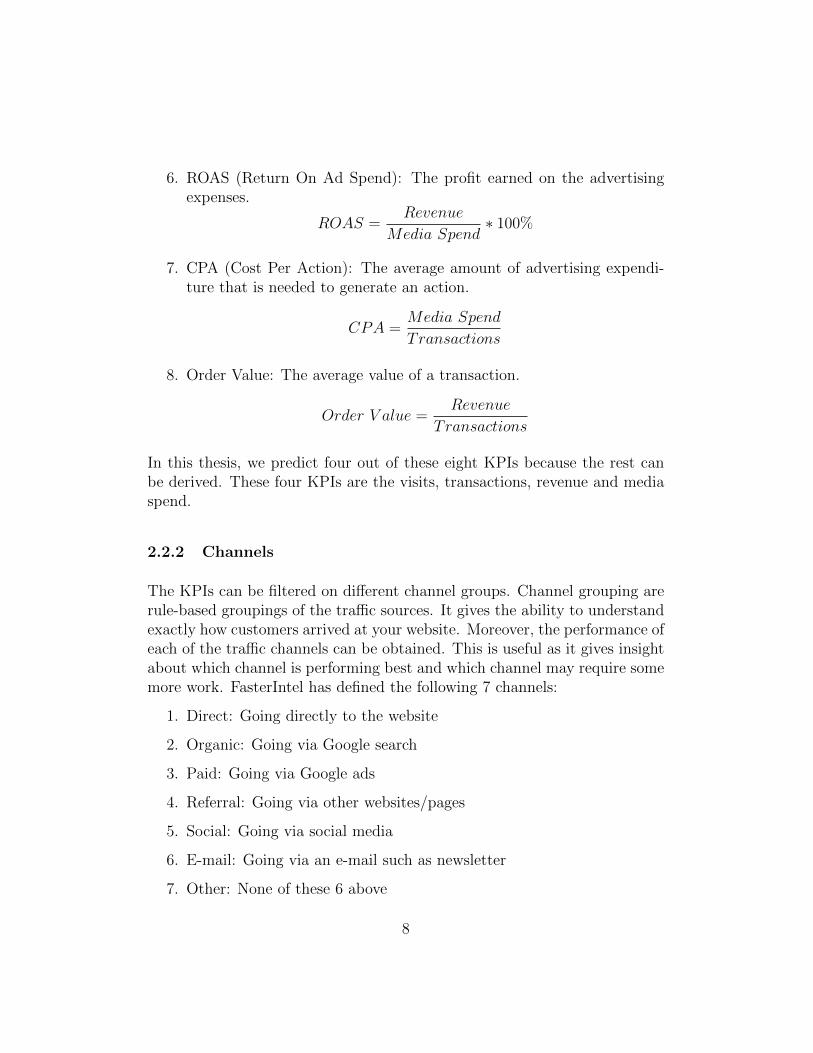

Data Description
DimensionsDate The date of the active date rangeSource The place users were before seeing your contentMedium Description of how users arrived at your content
MetricsTimeYear The year of the dateMonth The month of the dateWeek The week of the dateWeekday The weekday of the dateSeason The season of the date according to the four-season calendar reckon-
ingHoliday Variable indicating whether the date is a holiday in the NetherlandsKPIsSessions The total number of sessions (visits)Transactions The total number of completed purchases on the websiteRevenue The total revenue from web e-commerce or in-app transactionsAd Cost The total amount paid for advertising (media spend)AdvertisingImpression The number of times your ad is shown on a search result page or
other site on the Google networkAd Clicks The number of times someone clicks on your adActive campaigns The number of active campaignsSessionsBounce Rate The percentage of all sessions on your site in which users viewed only
a single page and triggered only a single request to the Analyticsserver
Percentage NewSessions
The percentage of sessions by users who had never visited the prop-erty before
Average SessionDuration
The average duration (in seconds) of usersrsquo sessions
UsersUsers The total number of users for the requested time periodNew Users The number of sessions marked as a userrsquos first sessionsSite SpeedAverage PageLoad Time
The average time (in seconds) pages from the sample set take to loadfrom initiation of the pageview to load completion in the browser
Average Redirec-tion Time
The average time (in seconds) spent in redirects before fetching thispage
Table 41 Google Analytics data and its description per day
The dataset consists of metrics for each day from 1 July 2014 to 31 May2017 for each corresponding source and medium The metrics can be dividedinto categories The time category consists of data that are derived from thedate The rest of the categories consists of data that are self explanatory
42 External Data
Besides the GA data external data is used This external data consistsof the weather inflation and the unemployment in the Netherlands Theweather data is obtained from Koninklijk Nederlands Meteorologisch Insti-tuut (KNMI) [19] and the others are obtained from Centraal Bureau voorde Statistiek (CBS) [20] The external data along with its description canbe found in Table 42 This external data could have an effect on the KPIsFor instance weather has an effect on consumer spending as shown in theliterature review
Data Description
WeatherAverage Temperature The average daily temperature (in 01 degree Celsius)Minimum Temperature The daily minimum temperature (in 01 degree Celsius)Maximum Temperature The daily maximum temperature (in 01 degree Celsius)Rainfall Amount The daily amount of rainfall (in 01 mm)Rainfall Duration The daily rainfall duration (in 01 hour)Sunshine Duration The daily sunshine duration (in 01 hours) calculated
from the global radiationInflationInflation Rate The monthly inflation rate (consumer price index) in
percentageUnemploymentUnemployment The percentage of unemployed (monthly)
Table 42 External data and their description
15
43 Data pre-processing
44 Data Analysis
In order to obtain insights from the data several analyses have been per-formed
From these analyses an overview of the time effect on the KPIs is obtained
The next analysis is the correlation between the KPI values and their ownlags This is analyzed using the autocorrelation function (ACF) and partialautocorrelation function (PACF) Both functions measure the correlation be-tween the current observation and an observation k time step ago but thepartial autocorrelation also takes into account the observations at intermedi-ate lags (ie at lags lt k) [21] They can be used to determine the magnitudeof the past values related to future values [10]
The ACF and PACF plots of the KPIs on the paid channel are shown inFigures 41 and 42
16
(a) Visits (b) Media Spend
(c) Transactions (d) Revenue
Figure 41 ACF plot of the KPIs on the paid channel The blue dashed linesindicate the point of statistical significance
17
(a) Visits (b) Media Spend
(c) Transactions (d) Revenue
Figure 42 PACF plot of the KPIs on the paid channel The blue dashedlines indicate the point of statistical significance
We observe that the ACF plot shows a slight peak at every 7th lag for allKPIs This indicates a weekly pattern The PACF plot shows a significantspike at lag 1 for all KPIs This indicates that the KPI value of previousday is very strong correlated with the value of current day For visits andmedia spend the lags 1 to 7 is significantly positive correlated Moreoverlag 8 is negative correlated and lags beyond 8 become less significant Fortransactions and revenue we observe significance until lag 7 followed by aspike at lag 14 that is caused by the weekly pattern
18
The final analysis is the exploration of the statistical relationship between theKPIs and the other metrics in the data The Pearson correlation between thedifferent variables in the data is computed Since we use past observations topredict the KPIs the correlation is between the current day KPIs value andthe metrics value of previous day except for weather inflation and unemploy-ment The values for weather are at the same day because weather forecastcan be derived from other resources This forecast can then be used as pre-dictor for the KPIs The value for inflation and unemployment is from theprevious month because daily observations are not available Even thoughthis is the case it can still help in daily forecast as inflation and unemploy-ment usually have a long term effect The correlation matrix for the paidchannel is shown in a correlogram in Figure 43
Figure 43 Pearson correlation matrix of the data on the paid channel
19
We observe correlations between KPIs themselves Visits (gasessions) ispositive correlated with media spend (gaadCost) which indicates that anincrease in media spend of the previous day results in an increase in next dayvisits Transactions is strong positive correlated with revenue (gatransactionRevenue)which is obvious The current day visits is strong correlated with previousday users and new users This can be explained by the fact that every singleuser generates at least one session Moreover a positive correlation is ob-served between visits and impressions and adClicks which shows the positiverelation between advertising and visits
For media spend we observe a positive correlation with impressions adclicksand number of active campaigns which is natural
With the obtained insights from the data analysis we have a good interpre-tation about which data can be used as features in the models This will befurther described in the experiments in section 62
20
5 Methods and Models
This section describes the models that are used for the forecast the multi-step forecasting method and the evaluation method
51 Models
511 Ratio-based model
The Ratio-based model is used as a benchmark model This model takes thehistorical data of a certain number of weeks before and computes the changein ratios over the same day for every week Next these ratios are averagedinto a single ratio and this single ratio is used as predictor for the next timestep
If we define Xt as the KPI at time step t and we take k weeks as historicaldata then the ratio change for Xt is given by
Ratiot =1
k
ksumi=1
Xt+1minus7i minusXtminus7i
Xtminus7i(51)
However problem occurs when the historical KPIs are zero ie Xtminus7i = 0for i = 1 k This will result in a division of zero which is not possibleTherefore in this case we take the difference of the KPIs instead of the ratio
Differencet =1
k
ksumi=1
Xt+1minus7i minusXtminus7i (52)
Moreover the difference forecast will be applied when Xt is zero as the ratioforecast will always result in a zero Thus the forecast on Xt+1 is given by
Xt+1 =
Xt lowast (1 + Ratiot) if Xt gt 0 or Ratiot is definedXt + Differencet if Xt = 0 or Ratiot is undefined
(53)
21
This equation expresses the single-step forecast The mathematical expres-sion for the recursive multi-step forecast is then
Xt+n =
nminus1prodi=0
(1 + Ratiot+i) lowastXt if Xt gt 0 or Ratiot+i is defined
nminus1sumi=0
Differencet+i +Xt if Xt = 0 or Ratiot+i is undefined
(54)
Notice that the ratio and the difference are always taken on the next timestep ie the ratio and difference between Xt and Xt+1 However we can alsotake the ratio and difference between multiple time steps ie between Xt andXt+n This will avoid the recursive strategy that usually has accumulatederror The ratio and the difference are then expressed as
Ratiot+n =1
k
ksumi=1
Xt+nminus7i minusXtminus7i
Xtminus7i
Differencet+n =1
k
ksumi=1
Xt+nminus7i minusXtminus7i
(55)
Next the non-recursive multi-step ahead forecast is given by
Xt+n =
Xt lowast (1 + Ratiot+n) if Xt gt 0 or Ratiot+n is definedXt + Differencet+n if Xt = 0 or Ratiot+n is undefined
(56)
The Ratio-based model for both the recursive and non-recursive multi-stepahead is illustrated in Figure 51
22
(a) Recursive forecast
(b) Non-recursive forecast
Figure 51 The Ratio-based model recursive and non-recursive forecastusing one week historical data The blue observations are the historicalobservations and the red observations are the forecast time steps
The advantage of this model is its simplicity and flexibility The model canbe easily implemented for all the KPIs and it is able to produce a forecasteven when little data is available The disadvantage is the reliability of themodel as large variation in KPIs over the weeks can easily result in inaccurateforecast
512 ARIMA
The ARIMA model is a stochastic time series model that combines threeprocesses the Autoregressive process (AR) the strip off of the integrated (I)time series by differencing and the Moving Averages (MA) [10] In an ARprocess the future value of a variable is assumed to be a linear combinationof p past observations plus a random error and a constant In a MA processthe past observations are the q past errors instead of the past observationsThus it is a linear combination of q past errors plus a random error and themean of the series These two processes can be combined together to forma more effective time series model This model is known as ARMA(pq) [22]and is given by
23
Xt = α1Xtminus1 + + αpXtminusp + εt + β1εtminus1 + + βqεtminusq (57)
where Xt is the observation at time t and εt is the random error at time tThis equation can be written implicitly as
(1minus
psumk=1
αkLk)Xt =
(1 +
qsumk=1
βkLk)εt (58)
where p and q are the order of the autoregressive and moving average partsof the model respectively and L is the lag operator
However ARMA can only be used for stationary time series ie the meanand variance of the time series do not depend upon time This is not the casein many time series such as in economic time series that contain trends andseasonal patterns Therefore the integrated term is introduced to include thecases of non-stationarity by applying differencing The difference operatortakes a differencing of order d and it is expressed as follows
∆dXt = (1minus L)dXt (59)
where Xt is the data point at time t L is the lag operator and d is the orderThus the three processes AR(p) I(d) and MA(q) are combined interactedand recomposed into the ARIMA(p d q) model
The general method to identify the order p in an AR process and q in aMA process is to use the autocorrelation function (ACF) and the partialautocorrelation function (PACF) [21] For a pure AR(p) process the PACFcuts down to zero after lag p For a pure MA(q) process the ACF cuts downto zero after lag q For ARMA(p q) and ARIMA(p d q) processes it is morecomplicated to estimate the parameters A method to do this is to performa grid search over these parameters using an evaluation metric for modelselection
24
513 Random Forest
Random Forest is a machine learning model for classification and regression[23] and it is illustrated in Figure 52
Figure 52 Random Forest [24]
Random Forest is an ensemble learning method that combines a group ofweak learners to form a more powerful model These weak learners are deci-sion trees and they can either be used for classification or regression In ourcase the focus is on regression
A decision tree is made up of decisions nodes terminal nodes (leaves) andbranches These branches represent the possible paths from one node toanother Decision trees are recursive partitioning algorithm that split thedataset in smaller subsets using a top-down greedy approach It starts atthe root node (top decision node) where a certain feature variable is usedto split the data into subsets Because the dataset can be split in numerousways the feature variable and its split point that yields the largest reductionin the residuals sum of squares (RSS) is chosen
Nsumn=1
sumiisinRn
(yi minus yn)2 (510)
where yi is the training observation i and yn is the mean of the responsevalues for the training observation that fall into the subset n
25
Next the decision tree recursively splits the dataset from the root nodeonwards at each decision node until the terminal nodes These terminalnodes are the endpoints of the decision tree and represent the final result ofa combination of decisions and events They are reached when all recordsafter the split belong to the same target variable or until a stopping criterionis met
In Random Forest a large number of these decision trees are constructed andeach tree makes a random selection of independent variables This results invariance in predictions between various decision trees which reduce overfittingand variance Then the prediction is produced by taking the mean predictionof the individual trees
Besides the number of trees in the forest it has other parameters that canbe varied such as the maximum depth of the tree the minimum number ofsamples required to split a decision node the minimum number of samplesrequired to be at a leaf node and the number of features to consider whenlooking for the best split
514 Artificial Neural Networks
ANNs are inspired by biological systems and the human brain and they haveshown powerful pattern classification and recognition capabilities [11] ANNslearn from experience by recognizing patterns in the input data Next theymake predictions based on their prior knowledge ANNs are applied in manydifferent fields of industry business and science [25] There are differenttypes of ANNs we have applied the feed-forward neural network (FNN) andthe recurrent neural network (RNN) [26 27] The FNN is the Multi-LayerPerceptron and the RNN is the Long Short-Term Memory
5141 Multi-Layer Perceptron
The Multi-Layer Perceptron (MLP) is a class of FNN Figure 53 illustratesthe architecture of a MLP
26
Figure 53 Architecture of a MLP with 3 layers (input hidden and output)with 4 input neurons 5 hidden neurons and 1 output neuron [28] Noticethat MLP can have multiple hidden layers
The network consists of processing elements also known as neurons that areorganized in layers Every neuron in a layer is connected with all the neuronsin the previous layers by acyclic links each with an associated weight Theseweights encode the knowledge of a network The neurons in the layers areused for transformation from input to output The output of each neuron yin the hidden layer(s) and output layer is a (non) linear function over the dotproduct of the weights of the connections with the outputs of the neurons inthe previous layer
y = φ
(sumi
ωixi + b
)(511)
Here xi are the inputs of the neuron ωi are the weights of the neuron and bis the bias φ is the activation function that determines the activation levelof the neuron
During training of the network the weights are modified such that the dif-ference between the network output and the actual output are minimized
27
Thus the estimation of the weights are based on the minimization of thecost function In our model this cost function is the mean squared errorIn order for the network to know how to adjust the weights it uses learningalgorithms The traditional learning algorithm is backpropagation [29] andit works as follows
1 Compute the feed-forward signals from the input to the output
2 Compute the error E of each neuron of the output layer using the costfunction
3 Backpropagate the error by the gradients of the associated activationfunctions and weighting it by the weights in previous layers
4 Compute the gradients for the set of parameters based on the feed-forward signals and the backpropagated error
5 Update the parameters using the computed gradients
∆ωij = αδjyi where (512)
δj =
φprime(vj)(tj minus yj) if j is an output nodeφprime(vj)
sumk of next layer δkωjk if j is an hidden node
Here ωij is the weight between node i and node j α is the learningrate yj is the output of node j vj is the activation of node j and tj isthe target output of node j
Even though backpropagation is used to solve many practical problems itshows problems such as slow convergence and getting stuck at local minima[29] Therefore other learning algorithms have been developed to improvethe performance of the backpropagation algorithm One of these learningalgorithms is the Adaptive Moment Estimation (Adam) [30] Adam is astochastic gradient descent algorithm based on estimation of first and secondorder moments of the gradients The algorithm works as follows
1 Compute the gradient using the current parameters
2 Update biased first order and second order moments estimate
mt = β1mtminus1 + (1minus β1)gtvt = β2vtminus1 + (1minus β2)g2t
(513)
28
Here mt is first order moment at time step t vt is the second ordermoment at time step t gt is the gradient at time step t and g2t indicatesthe element-wise square of gt β1 and β2 are the exponential decay ratesbetween 0 and 1
3 Compute the bias-corrected first and second order moments
mt =mt
1minus βt1
vt =vt
1minus βt2
(514)
4 Compute weight update and update parameters
θt = θtminus1 minus αmt
(radicvt + ε)
(515)
Here θt is the parameter vector at time step t and α is the learningrate
Adam computes adaptive learning rates for each parameter [31] that speedsup the learning phase This leads to faster convergence Furthermore littlemanual tuning of hyperparameters are required because they have intuitiveinterpretation All these advantages are beneficial for all the models thatneed to be constructed Therefore Adam is used as learning algorithm
5142 Long Short-Term Memory
In FNNs information is only propagated in one direction This is in contrastto recurrent neural networks (RNNs) where information is propagated in bi-directions using feedback loops These feedback loops transfer internal andoutput signals back to the input level which allows information to persistThus a RNN has an internal memory that captures information about whathas been calculated so far This becomes clear if we unfold the RNN throughtime as shown in Figure 54
29
Figure 54 A RNN unfolded in time [32] Here U V W represent the set ofweights xt is the input at time step t st is the hidden state at time step tand ot is the output at time step t
Therefore RNNs can model temporal dependencies of unspecified durationbetween the inputs and the associated desired outputs [33] Because of thisRNNs are suitable for time series predictions However when the gap be-tween the relevant information and the prediction becomes larger regularRNNs become unable to learn to connect the information because of thevanishing gradients (ie the gradient gets so small that learning either be-comes very slow or stops) The problem of vanishing gradients can be avoidedusing Long Short-Term Memory (LSTM)
LSTM is a specific RNN that is capable of learning long-term dependenciesand it was introduced by Hochreiter and Schmidhuber [34] The networktakes three inputs The input Xt of the current time step t the output fromthe previous LSTM unit htminus1 and the memory of the previous unit Ctminus1
The LSTM unit contains special units called memory blocks in the recurrenthidden layer An individual memory block is shown in Figure 55 Eachmemory block contains memory cells and three gated cells that is shared byall the memory cells These three gates are the forget input and output gateand control the information flow to the cells The forget gate decides whatinformation will be removed in the memory The input gate decides whatinformation will be updated The output gate defines what information insidethe cells will be exposed to the external network These gates are controlledby a simple one layer neural network using the sigmoid activation functionThus the network outputs a value between 0 and 1 where 0 represents closed
30
gates and 1 represents open gates
Figure 55 A single LSTM memory block [35]
The forget and input gate use the three LSTM network inputs Xt htminus1 andCtminus1 and a bias vector as input The output gate uses the htminus1 Xt the newmemory Ct and a bias vector as input Thus the forget gate ft input gateit and output gate ot of the current time step t is given by the followingequations
ft = σ(bf +WxfXt +Whfhtminus1 +WcfCtminus1)
it = σ(bi +WxiXt +Whihtminus1 +WciCtminus1)
ot = σ(bo +WxoXt +Whohtminus1 +WcoCt)
(516)
Here σ is the sigmoid function b is the bias vector and W represents the setof weights
The new memory Ct is also generated by a simple neural network but it usesthe hyperbolic tangent as activation function instead of the sigmoid functionThe new memory Ct is then generated by element-wise multiplication of theinput gate it and by adding the old memory Ctminus1
31
Ct = ftCtminus1 + it tanh(bc +WxcXt +Whchtminus1) (517)
Here tanh is the hyperbolic tangent function b is the bias vector and Wrepresents the set of weights
The output ht for the LSTM unit is then generated using the new memoryCt that is controlled by the output gate ot
ht = ot tanh(Ct) (518)
Again the weights in the network need to be learned The learning algorithmAdam is used for this purpose because it can handle the complex training dy-namics of RNNs better than plain gradient descent [30] Moreover since thenetwork uses the hyperbolic tangent function as activation function whichis bounded between -1 and 1 the data is normalized between -1 and 1
52 Multi-step Forecasting Strategies
Since FasterIntel always shows predictions of the KPIs up to Sunday (endof the week) for each week it means that it requires a maximum of 7 daysahead forecast Therefore we decided to forecast the KPIs always 7 timesteps ahead on each day Predicting multiple time steps into the future isalso known as multi-step time series forecasting Different strategies are usedfor multi-step time series forecasting [36] The most common strategies arethe direct multi-step forecast and the recursive multi-step forecast The di-rect multi-step forecast uses a separate model for each forecast time stepwhile the recursive multi-step forecast uses a one-step model multiple timesIt takes the prediction for the prior time step as an input for making a pre-diction on the following time step A disadvantage of the recursive strategyis the accumulation of the prediction errors as the forecast horizon increaseswhile this does not hold in the direct strategy However this does not meanthat the direct strategy is always better than the recursive strategy It alldepends on the model specification Another disadvantage of the recursivestrategy are the unknown values for other time series when they are usedas predictors This means that each time series need to be predicted Thedisadvantage of the direct strategy is that it involves a heavier computationalload than the recursive strategy Moreover since the direct strategy forecasts
32
each time step in isolation of the other time steps it can produce completelyunrelated forecasts over the whole forecast horizon This can lead to un-realistic discontinuities whereas time series have some aspect of continuousbehavior in reality [37] Therefore the recursive strategy is applied in thisresearch
53 Evaluation
The performance of the models is evaluated using the time series cross vali-dation This process is illustrated in Figure 56
Figure 56 The series of training and test sets in time series cross validationThe blue observations form the training sets and the red observations formthe test sets [38]
This validation has a series of training and test sets Each of the test setsconsists of n observations that corresponds with the n time step ahead fore-cast The corresponding training set consists of features that occurred priorto the first observation of the test set This mimics the real-world scenariowhere new observations become available for each time step t Next thisvalidation method walks each series of the test sets one at a time and makesn predictions for each time step
Next the real observations and the predictions for each time step are com-pared with each other using an error measurement The error measurementthat is used is the Root Mean Squared Error (RMSE) and it is given by
33
RMSE =
radicradicradicradic 1
m
msumi=1
(yi minus yi)2 (519)
Here yi is the predicted value for observation i yi is the actual value forobservation i and m is the total number of observations
The RMSE penalizes extreme errors as it is much affected by large individualerrors Thus we obtain n RMSE values where each of these values representsthe error for a single time step t t+ 1 t+ n
34
6 Experimental Setup
This section describes the training and testing of the models the two exper-iments that are conducted and the optimization of the model hyperparame-ters
61 Training and Testing
Since the KPIs have seasonality within a year as shown in the analysis insection 44 it is important that the models are evaluated on at least one yeartest data to capture their overall performance Therefore we chose the last365 days of the dataset as test set starting from 25 May 2016 Notice thatit does not start from 31 May 2016 because observations after 31 May 2017are not available in the dataset when performing 7 days ahead forecast
The models are retrained after each 30 series This corresponds with retrain-ing the model every month The decision to not retrain the models every dayis because retraining on one new observation in the training set will hardlymake any difference in terms of performance
62 Experiments
In this research two experiments have been conducted These experimentsare categorized into experiment A and experiment B
621 Experiment A
In experiment A the data used for each KPI forecast are the correspondinghistorical KPI data along with time related data The time related data arethe month week weekday season and holiday The choice of performing thisexperiment is because the current forecast model only uses the correspondinghistorical KPI data Thus it is interesting for FasterIntel to know about thepredictive performance of each model using only this data The time relateddata is used to capture temporal information from the time series for RandomForest and MLP because they are non-temporal models This is in contrast
35
with ARIMA and LSTM which are temporal models that should be able tocatch temporal information automatically from the time series Thus theinput data for ARIMA and LSTM are only the lagged values of the KPIunder investigation whereas Random Forest and MLP added additional timerelated data and the weekly moving average of the KPI as input to spot theweekly trend
The total number of lags to consider in each model are determined in differentways depending on the model In ARIMA the number of lags is the orderp in the AR part and q in the MA part This order is determined using agrid search method on the validation set that will be described in section63 In LSTM a lag of one is used because information of the lags are passedthrough each recurrent state to the next state In Random Forest and MLPthe number of lags are based on the PACF analysis in section 44 For visitsand media spend the first 8 lags are used and for transactions and revenuethe first 7 lags and the 14th lag are used
Random Forest and ANNs are run for multiple times and the average perfor-mance was taken as final performance for the models This is because thesemodels are stochastic and therefore they return different results on differentruns of the same algorithm on the same data
622 Experiment B
In experiment B all the data are used in the KPIs forecast With this ex-periment we are able to show the difference in performance compared toexperiment A when more data is added This could be interesting for Fas-terIntel as they can set up new businesses with their clients eg offeringbetter KPIs predictive performance for only premium clients However weonly forecast one step ahead instead of multi-step ahead because it becomescomputationally too intensive when additional time series features are addedThe reason is that the recursive strategy requires predictions for every addi-tional time series feature and developing models to do so was out of scopein this thesis Notice that ARIMA is excluded in this experiment as it is aunivariate time series model
In order to ensure that the difference in performance is caused by addingadditional features the same features in experiment A plus the additional
36
features are used These additional features are chosen based on the analysisof the Pearson correlation matrix as shown in Figure 43 The additionalfeatures for the KPIs are shown in Table 61
KPI Additional Features
Visits rdquoad costrdquo rdquousersrdquo rdquonew usersrdquo rdquoimpressionrdquordquoinflationrdquo rdquounemploymentrdquo
Transactions rdquoad costrdquo rdquousersrdquo rdquonew usersrdquo rdquoimpressionrdquordquoaverage temperaturerdquo rdquomaximum temperaturerdquordquoinflationrdquo rdquounemploymentrdquo
Revenue rdquoad costrdquo rdquousersrdquo rdquonew usersrdquo rdquoimpressionrdquordquoaverage temperaturerdquo rdquomaximum temperaturerdquordquoinflationrdquo rdquounemploymentrdquo
Media Spend rdquoimpressionrdquo rdquocampaignsrdquo rdquoad clicksrdquo
Table 61 KPI and its additional features
Again the number of lags for each feature had to be determined in the inputdata as in experiment A Zero lag is chosen for the temperature data as yourcurrent behaviour can be influenced by the current weather condition Alag of one is chosen for the other additional features because it is the mostrepresentative for the current time step Moreover the moving average of 7days for all Google Analytics features and the weather is included which giveinformation about the weekly trend of each time series feature
63 Hyperparameters Optimization
ARIMA Random Forest MLP and LSTM all have hyperparameters thatneed to be optimized to achieve good performance The hyperparametersin ARIMA are the auto regressive order p the integration order d and themoving average order q For Random Forest MLP and LSTM not all hyper-parameters are considered The ones that are considered in Random Forestare the number of trees in the forest the number of features to consider whenlooking for the best split and the minimum sample leaf size The hyperpa-rameters that are considered in MLP are the number of hidden layers andneurons in each layer and the activation functions The hyperparameters
37
that are considered in LSTM are the number of hidden layers and LSTMunits in each layer
All the combinations of the hyperparameters were tested on the validationset This validation set is a separation of the first training set in the timeseries cross validation and contains one month of data starting from 25 April2016 to 24 May 2016 Thus the models were trained on the data before 25April 2016 Next each model was trained again on the whole first trainingset using the optimal hyperparameters and evaluated using time series crossvalidation as described in section 53
The hyperparameter optimization for ARIMA was performed using a gridsearch method This method tries every hyperparameter setting over a spec-ified range of values The search range for the autoregressive order p andmoving average order q was set based on the PACF and ACF analysis insection 44 respectively For the autoregressive order p it was set from 0 to8 for visits and media spend and from 0 to 14 for transactions and revenueFor the moving average order q it was set from 0 to 7 for all the KPIs Thesearch range for the integration order d was set from 0 to 1 The choice fora maximum of first order differencing is because second order differencing israrely needed to achieve stationarity [10]
In Random Forest the optimal number of trees was determined to be inthe range from 10 to 400 and the optimal minimum sample leaf size wasdetermined to be in the range from 1 to 50
In MLP the optimal hidden neurons in each hidden layer was determined inthe range 10 to 100 The number of hidden layers was set to a maximum oftwo layers The rectified linear unit (ReLU) activation function was used inthe hidden layers because it was found to be the most efficient when appliedto the forecasting of non-stationary and noisy time series Next the linearactivation function was used in the output layer to output the forecast valueof the time series
In LSTM the number of hidden layers was set to one and the number ofLSTM units was determined in the range 10 to 40 The exponential decayrates β1 and β2 were set to default values of 09 and 0999 respectively Thesedefault values are proposed in the original paper [34]
38
7 Results
In this section the results of the two experiments are presented First section71 presents the results for experiment A and it contains results with regardsto model hyperparameters model performance model comparison and fea-ture importance Next section 72 presents the results for experiment Band it contains results with regards to model hyperparameters model per-formance and feature importance Finally section 73 summarizes the resultsof both experiments
71 Experiment A
711 Hyperparameters
The results for the hyperparameters for ARIMA Random Forest and MLPare shown below
39
ARIMA
Figure 71 ARIMA Order(p d q)2
Figure 71 shows the RMSE for different combinations of order(p d q) Weobserve many fluctuations in errors for the different combinations The op-timal order achieved for visits transactions revenue and media spend is(605) (202) (402) and (706) respectively
2The order(p d q) starts at (000) and is first incremented for q next for d and as lastfor p
40
Random Forest
Figure 72 Random Forest Number Of Trees
Figure 72 shows the RMSE for different number of trees We observe thatthe optimal number of trees for visits is 270 as increasing the number oftrees will not significantly decrease the RMSE anymore For transactionsthe RMSE becomes stable after 120 trees The number of trees that is chosenfor revenue and media spend is 300 and 370 respectively It is not necessaryto increase the number of trees further as the performance stays roughly thesame while the computational time will increase
The optimal maximum number of features to look for the best split wasfound to be the square root of the number of input features The optimalminimum sample leaf size in experiment A was 7 2 3 and 2 for visitstransactions revenue and media spend respectively In experiment B theoptimal minimum sample leaf size was 4 1 4 and 1 for visits transactionsrevenue and media spend respectively
41
MLP
Figure 73 MLP number of hidden layers and hidden neurons
Figure 73 shows the RMSE for different number of hidden layers and hiddenneurons in the training and validation set We observe that the error of thetraining set in visits transactions and revenue is larger than the error inthe validation set This is caused by the different cases in both sets Thetime series in the training set contains data over multiple months whereasthe time series in the validation set contains only data over one month Theseasonality over the different months causes that some months are harder tolearn than other months
We observe a linear decrease in the error of the training set when two hiddenlayers are applied for visits However this is not observed in the validationset The errors are rather stable over the different number of hidden layersand neurons The lowest error is achieved using two hidden layers with 10
42
neurons in each layer For media spend and revenue the use of two hiddenlayers is also sufficient both errors in the training set and validation setdecrease when the number of neurons is increased The error becomes almostconstant after 70 neurons in both layers for media spend and after 60 neuronsin both layers for revenue The lowest error in the validation set is achievedusing two hidden layers with 100 neurons in each layer for media spend andtwo hidden layers with 90 neurons in each layer for revenue For transactionsone hidden layer with 20 neurons gives the smallest error in the validationset
43
LSTM
Figure 74 LSTM number of units
Figure 74 shows the RMSE for different number of LSTM units on thetraining and validation set We observe again that the training set error islarger than the validation error Moreover increasing the number of LSTMunits does not really improve the training set error whereas the validationerror for some KPIs increases The validation error increases after 20 LSTMunit for visits and media spend The validation error for transactions andrevenue are relatively stable for different number of LSTM units The lowesterror is achieved using 10 LSTM unit for transactions and 20 LSTM unit forrevenue
44
712 Model Performance
The performance of each model using the time series cross validation on thepaid channel over 10 runs is shown in Figure 75
Figure 75 Model performance on the paid channel
The Ratio-based model is excluded in transactions and revenue because theerror is off the scale that made the other models not comparable anymoreThe exact values of the RMSE is also shown in tables in Appendix B
We observe that ARIMA MLP and Random Forest outperform the linearregression model (current model) for the four KPIs ARIMA and RandomForest both perform well for visits However MLP starts to perform betterthan ARIMA and Random Forest after time step t+ 4 For media spend weobserved the opposite where MLP performs better until time step t+ 3 andgets bypassed by Random Forest after time step t+3 Random Forest showsthe best performance for transactions and MLP shows the best performancefor revenue The Ratio-based model has the worst performance of all themodels and LSTM performed the worst when comparing to ARIMA MLPand Random Forest These results will be discussed in the discussion insection 8
713 Feature Importance
After training the Random Forest we can obtain their feature importanceand this is shown in Figure 76 for the paid channel
45
Figure 76 Feature Importance of Random Forest on the paid channel
We observe that for visits and media spend the most important feature istminus 1 (lag 1) This means that previous day value is important in predictingthe value on the next day Moreover the moving average shows importancein all the KPIs that give information about trends or cycles Interestingto observe is that lag 8 (t minus 8) shows little importance comparing to theother lags while it shows a strong correlation in the PACF plot in Figure 42Furthermore the model performance is barely affected when lag 8 is removedfrom the model
46
714 Model Comparison
Based on the model performance in Figure 75 we can already compare themodels with each other However to ensure that these model performanceresults are statistically significant the squared errors of the models are testedusing the two-sided Kolmogorov-Smirnov test (K-S test) The two-sidedK-S test is used to test whether two independent samples are drawn fromthe same continuous distribution In our case we are testing whether thesquared errors per instance of two different models are drawn from the samecontinuous distribution This is also known as the KS Predictive Accuracy(KSPA) test [39] Thus we test the null hypothesis
H0 The squared error of model A and model B
come from the same continuous distribution
against the alternative hypothesis
H1 The squared error of model A and model B
do not come from the same continuous distribution
The test is performed for all the forecast horizon However the result fortime step t is only shown here for clarity For visits we obtained the followingp-values between the different models as shown in Table 71
p-value Linear RatioRec
RatioNonRec
ARIMA RandomForest
MLP LSTM
Linear 1 157e-24 157e-24 149e-21 125e-26 123e-15 454e-19RatioRec
157e-24 1 1 216e-05 326e-05 307e-05 132e-09
RatioNonRec
157e-24 1 1 216e-05 326e-05 307e-05 132e-09
ARIMA 149e-21 216e-05 216e-05 1 186e-03 019 321e-03RandomForest
125e-26 326e-05 326e-05 186e-03 1 543e-03 140e-08
MLP 123e-15 307e-05 307e-05 019 543e-03 1 543e-03LSTM 454e-19 132e-09 132e-09 321e-03 140e-08 543e-03 1
Table 71 The p-values from the KSPA test between the models for the KPIvisits for time step t
47
If we assume a significance level of 95 (p-value less than 005) we observethat most of the p-values are significant The only insignificant one is thedistribution of the squared errors between ARIMA and MLP with a p-valueof 019 This means that we cannot reject the null hypothesis and the squarederrors are likely to come from the same distribution This is unexpected asthe RMSE for ARIMA is much lower than MLP as observed in Figure 75Further analysis we found that the empirical distribution of the squarederrors of ARIMA and MLP look almost the same but that MLP contains afew much larger errors than ARIMA This caused the larger RMSE for MLPNext the same analysis is performed for transactions and the result is shownin Table 72
p-value Linear ARIMA RandomForest
MLP LSTM
Linear 1 069 050 045 013ARIMA 069 1 099 099 098RandomForest
050 099 1 1 099
MLP 045 099 1 1 098LSTM 013 098 099 098 1
Table 72 The p-values from the KSPA test between the models for the KPItransactions for time step t
We observe that none of the p-values are significant This indicates thatthe errors for all the models come from the same distribution From theRMSE as shown in Figure 75 we already observe that the difference betweenthese models are very small This difference is mostly caused by the severallarge transactions in the testset where Random Forest predicts these largetransactions the closest
The p-values for revenue are also insignificant for all the models as shownin Table 73 The difference in RSME is also caused by the outliers in thetestset where MLP predicts these the closest
48
p-value Linear ARIMA RandomForest
MLP LSTM
Linear 1 056 022 022 022ARIMA 056 1 030 016 045RandomForest
022 030 1 063 091
MLP 022 016 063 1 030LSTM 022 045 091 030 1
Table 73 The p-values from the KSPA test between the models for the KPIrevenue for time step t
Table 74 shows the p-values between the models for the media spend Weobserve that most of them are significant and the insignificant ones are theerrors between Random Forest and MLP Random Forest and ARIMA andMLP and ARIMA with p-values 063 063 and 045 respectively Moreoverthe difference in RMSE between these models is small as shown in Figure75 Thus it is expected that these squared errors come from the samedistribution
p-value Linear RatioRec
RatioNonRec
ARIMA RandomForest
MLP LSTM
Linear 1 125e-26 125e-26 350e-29 620e-30 119e-34 658e-16RatioRec
125e-26 1 1 001 004 001 556e-09
RatioNonRec
125e-26 1 1 001 004 001 556e-09
ARIMA 350e-29 001 001 1 063 045 129e-07RandomForest
620e-30 004 004 063 1 063 347e-09
MLP 119e-34 001 001 045 063 1 198e-07LSTM 658e-16 556e-09 556e-09 129e-07 347e-09 198e-07 1
Table 74 The p-values from the KSPA test between the models for the KPImedia spend for time step t
When the KSPA test was applied for the other forecast horizons We found
49
for visits that the forecast generated by ARIMA and MLP are not statisticallydifferent from each other for all time steps Moreover the squared errorbetween Random Forest and MLP and the squared error between RandomForest and ARIMA become insignificant after time step t with p-value of010 and 06 respectively This mean that there is no significant differencebetween these three models after time step t
For transactions we found that neither of the models are statistically sig-nificant different from each other for all the forecast horizon This meansthat all models are suitable for forecasting transactions The reason is thatthe variance of transactions is relatively small which makes the forecast errorrelatively similar for all models
For revenue we also found that neither of the models are statistically sig-nificant different from each other for all the forecast horizon This whilewe observe a significant difference in RMSE between some models over theforecast horizon The difference is caused by large revenues that is bettercaptured by some models
For media spend we found that the forecast error between ARIMA andRandom Forest becomes statistically significant after time step t+4 (p-valueof 004) Random Forest is then performing statistically better than ARIMAFurthermore the forecast error of MLP and Random Forest are insignificantfor all time steps which means that they are both performing the same
50
72 Experiment B
721 Hyperparameters
The hyperparameters need to be optimized as in experiment A The samenumber of trees was used as in experiment A because the same behaviour wasobserved in experiment B However this same behaviour was not observedfor the number of neurons in the neural networks In this experiment moreneurons were needed in the neural networks because of the increased numberof inputs The change of the number of neurons in MLP is shown in Table75 and the change of number of LSTM units is shown in Table 76
MLP Experiment A Experiment B
Visits 1010 2020Transactions 20 40Revenue 9090 100100Media Spend 100100 100100
Table 75 The optimal neurons in the hidden layers for experiment A and B
LSTM Experiment A Experiment B
Visits 20 20Transactions 10 40Revenue 10 30Media Spend 20 40
Table 76 The optimal LSTM units for experiment A and B
722 Model Performance
The performance of the models are obtained over 10 runs and the resultalong with the result from experiment A are presented Table 77 shows theRMSE for Random Forest in both experiments and its p-value of the KSPAtest between the squared error of the model in the two experiments
51
Table 77 The RMSE of time step t on the paid channel using RandomForest of experiment A and B and its p-value of the KSPA test
We observe that the RMSE in experiment B does not differ significantly fromthe RMSE in experiment A for all KPIs This is also confirmed by the KSPAtest as non of the p-values are significant Thus the additional features arenot contributing in improving the performance The reason is that theseadditional features are largely irrelevant that will be shown in the featureimportance in Figure 77
Next the result for MLP is shown in Table 78
Table 78 The RMSE of time step t on the paid channel using MLP ofexperiment A and B and its p-value of the KSPA test
The same result as in Random Forest is observed here The performance isnot improving and it is almost the same as experiment A This behaviour isalso observed in LSTM as shown in Table 79 From the results it becomesclear that it has no benefit to add the additional features as the performanceis not improving
Table 79 The RMSE of time step t on the paid channel using LSTM ofexperiment A and B and its p-value of the KSPA test
723 Feature Importance
The feature importance for Random Forest can again be derived to obtainthe importance of the additional features The result is shown in Figure 77
52
Figure 77 Feature Importance of Random Forest including additional fea-tures on the paid channel
We observe for visits that the features rdquousersrdquo and rdquonew usersrdquo are quiteimportant because they have a very strong correlation with visits as shownin Figure 43 rdquoAd costrdquo and rdquoimpressionrdquo on the contrary shows little im-portance
The most important features in media spend are still the same features inexperiment A The additional features rdquoimpressionrdquo rdquoad clicksrdquo and rdquocam-paignsrdquo show little importance
The moving average is still the top important feature in transactions and
53
revenue The additional features seem to have an importance but they areall below 008 which indicates a very low importance
73 Summary
From the results of both experiments we obtained that adding the additionalfeatures in experiment B did not result in improvement Moreover when westatistically compared the performance of the models using the KSPA testsome of the models were insignificant while there was a significant differencein RMSE Further analysis we found out that this difference was caused bysome outliers in the testset Some of the models predicted these outliersbetter than others The model with the lowest error for each KPI performedbetter than the current model The best model for each KPI along with itsaverage improvement over the time steps on the paid channel is shown inTable 710
KPI Best Model Improvement
Visits Random Forest 4175Transactions Random Forest 1704Revenue MLP 1702Media Spend MLP 5600
Table 710 The best models for each KPI on the paid channel and theirimprovement with respect to the current model
Transactions and revenue have the smallest improvement because these arethe hardest to predict The media spend has the greatest improvement How-ever the RMSE of these best models are still large when they are comparedto the magnitude of the values in the test set
54
8 Discussion and Conclusion
The implemented models except the Ratio-based model were able to improvethe forecast of the current model The Ratio-based model resulted in hugeerrors as the variability between the same days over the weeks are large Eventhough improvement is made the performance is still not outstanding Theproblem is not caused by the implemented models but the limited amountof historical data and features available We only have data for three yearswhere one year was already used for testing Thus training on two years ofhistorical data is just too small for the models to learn and understand thedata This especially holds for complex models like neural networks wheremore training data are needed for them to generalize This may explain thebad performance of LSTM whereas ARIMA and Random Forest require lessdata to generalize Moreover the validation set consists of only one monthdata instead of one year that could give the wrong optimal hyperparametersHowever if one year of data is taken as validation set then only one yearof data remains for the training set This is inadequate for training a goodmodel as the yearly patterns cannot be captured Besides the limited datathe recursive strategy can play a role in the performance of the multi-stepahead forecast From the results we have observed that the error increasesalong with the time horizon This error might be reduced when using thedirect strategy
From experiment A we obtained that it is hard to make accurate predictionsof the KPIs based on only their own past values Therefore we includedexternal data that is still applicable for all clients and other Google Analyticsfeatures in experiment B However they have shown less predictive valueMoreover the external data was coarse grained except for weather whichmakes it less valuable for daily forecast Based on the feature importancethe moving average has shown to be always on the top 3 most importantfeature because it captures the overall trend of the KPIs over the time stepsHowever neither of the most important feature exceeded an importance valueof 025 This indicates that the data have low predictive value and other dataare needed
Data that could improve the performance is internal company data How-ever these data cannot be derived from Google Analytics Data such asinformation about the products they offer Relevant information such as
55
the price rating reviews and discounts This information could help in theprediction of transactions and revenue as shown in the literature reviewMoreover information about their upcoming media strategy can be relevant[40] This will all have an impact on the performance of the KPIs Besidesonline marketing offline marketing is also used to increase awareness suchas informative pamphlets flyers television and radio advertising and mag-azines [41] In conclusion internal company data might be important asthey describe the behaviour of KPIs more explicitly However this suggeststhat we have to acquire these data that is not generic anymore and does notmatch with the product point of view Thus there is a trade off betweenperformance and scalability High performance can be acquired when moreattention is paid on each client [42] However this will result in higher costand more time from the business side
Based on this research we would recommend to be cautious with using onlyGoogle Analytics data to forecast the KPIs because limited knowledge canbe gained from this Moreover it is dangerous when marketeers rely on thesebad predictions to take actions because this will lead to wrong actions Forfuture research it would be interesting to acquire company internal dataand more history if available This data together with Google Analyticsdata can then be applied and might improve the KPIs prediction furtherFurthermore we have only focused on the paid channel in this research Itmight be also interesting for future research to forecast the KPIs on the otherchannels Channels that are less affected by advertising such as the directchannel might be easier to predict
The formulated research question was rdquoWith how much can the forecastof KPIs be improved compared to the current model using only data that isgeneric enough to be available from all clientsrdquo The findings in this researchshow that the forecast of visits improved with 42 transactions and revenuewith 17 and media spend with 56 However the prediction error is stilllarge for all KPIs The reason is that generic data can only capture genericinformation on the KPIs whereas many other specific factors can affect theseKPIs Therefore it is really difficult to make accurate predictions using onlygeneric information
56
References
[1] Shuojia Guo and Bingjia Shao ldquoQuantitative evaluation of e-commercialWeb sites of foreign trade enterprises in Chongqingrdquo In 1 (June 2005)780ndash785 Vol 1
[2] statista Retail e-commerce sales worldwide from 2014 to 2021 (in bil-lion US dollars) httpswwwstatistacomstatistics379046worldwide-retail-e-commerce-sales
[3] Alanah J Davis and Deepak Khazanchi ldquoAn Empirical Study of OnlineWord of Mouth as a Predictor for Multi-product Category e-CommerceSalesrdquo In 18 (May 2008) pp 130ndash141
[4] C Ranganathan and Elizabeth Grandon ldquoAn Exploratory Examina-tion of Factors Affecting Online Salesrdquo In Journal of Computer Infor-mation Systems 423 (2002) pp 87ndash93
[5] Qiang Ye Rob Law and Bin Gu ldquoThe Impact of Online User Reviewson Hotel Room Salesrdquo In 28 (Mar 2009) pp 180ndash182
[6] James W Taylor ldquoForecasting daily supermarket sales using exponen-tially weighted quantile regressionrdquo In European Journal of Opera-tional Research 1781 (2007) pp 154ndash167
[7] Besta P Lenort R ldquoHierarchical Sales Forecasting System for ApparelCompanies and Supply Chainsrdquo In 21 (2013) pp 7ndash11
[8] Ilan Alon Min Qi and Robert J Sadowski ldquoForecasting aggregateretail sales a comparison of artificial neural networks and traditionalmethodsrdquo In Journal of Retailing and Consumer Services 83 (2001)pp 147ndash156
[9] Gareth James et al An Introduction to Statistical Learning With Ap-plications in R Springer Publishing Company Incorporated 2014
[10] By George E P Box et al Time Series Analysis Forecasting and Con-trol Vol 68 Jan 2016 isbn 978-1-118-67502-1
[11] GPZhang ldquoNeural Networks for Time-Series Forecastingrdquo In Hand-book of Natural Computing (2012) pp 461ndash477
[12] Vincent Cho ldquoA comparison of three different approaches to touristarrival forecastingrdquo In Tourism Management 243 (2003) pp 323ndash330
[13] F M Thiesing and O Vornberger ldquoSales forecasting using neuralnetworksrdquo In Neural Networks1997 International Conference on 4(1997) 2125ndash2128 vol4
57
[14] Peter vd Reijden and Otto Koppius ldquoTHE VALUE OF ONLINEPRODUCT BUZZ IN SALES FORECASTINGrdquo In International Con-ference on Information Systems (2010)
[15] Kris Johnson Ferreira Bin Hong Alex Lee and David Simchi-LevildquoAnalytics for an Online Retailer Demand Forecasting and Price Op-timizationrdquo In Manufacturing amp Service Operations Management 181(2016) pp 69ndash88
[16] P Meulstee and M Pechenizkiy ldquoFood Sales Prediction rdquoIf Only ItKnew What We Knowrdquordquo In 2008 IEEE International Conference onData Mining Workshops (2008) pp 134ndash143
[17] Kyle B Murray et al ldquoThe effect of weather on consumer spendingrdquoIn Journal of Retailing and Consumer Services 176 (2010) pp 512ndash520
[18] Google Analytics Solutions httpswwwgooglecomanalyticsanalyticsmodal_active=none
[19] KlimatologieDaggegevens van het weer in Nederland httpprojectsknminlklimatologiedaggegevensselectiecgi
[20] Centraal Bureau voor de Statistiek StatLine httpstatlinecbsnlStatwebLA=nl
[21] Ratnadip Adhikari and R K Agrawal An Introductory Study on Timeseries Modeling and Forecasting Jan 2013 isbn 978-3-659-33508-2
[22] BChoi ARMA Model Identification Springer Series in Statistics 1992isbn 978-1-4613-9745-8
[23] TK Ho ldquoRandom decision forestsrdquo In In Document Analysis andRecognition (1995) pp 278ndash282
[24] Dan Benyamin A Gentle Introduction to Random Forests Ensemblesand Performance Metrics in a Commercial System httpblog
citizennetcomblog20121110random-forests-ensembles-
and-performance-metrics[25] MA Lehr BWidrow DERumelhart ldquoNeural networks Applications
in industry business and sciencerdquo In Communications of the ACM(1994) pp 93ndash105
[26] Z Tang and PA Fishwick ldquoFeedforward Neural Nets as Models forTime Series Forecastingrdquo In ORSA Journal on Computing (1993)pp 374ndash385
[27] G Dorffner ldquoNeural Networks for Time Series Processingrdquo In 6 (1996)[28] J Cazala Perceptron https github com cazala synaptic
wikiArchitect
58
[29] R Hecht-Nielsen ldquoTheory of the backpropagation neural networkrdquo In(1989) 593ndash605 vol1
[30] PDKingma and JLBa ldquoAdam a method for stochastic optimiza-tionrdquo In ICLR (2015)
[31] Sebastian Ruder ldquoAn overview of gradient descent optimization algo-rithmsrdquo In (Sept 2016)
[32] D Britz Recurrent Neural Networks Tutorial Part 1 ndash Introductionto RNNs httpwwwwildmlcom201509recurrent-neural-networks-tutorial-part-1-introduction-to-rnns
[33] M Assaad and R Bone ldquoA new boosting algorithm for improved time-series forecasting with recurrent neural networksrdquo In Information Fu-sion 91 (2008) pp 41ndash55
[34] Sepp Hochreiter and Jurgen Schmidhuber ldquoLong Short-term Mem-oryrdquo In 9 (Dec 1997) pp 1735ndash80
[35] colah Understanding LSTM Networks httpblogotoronet
20150514long-short-term-memory[36] SB Taieb and RJ Hyndman ldquoRecursive and direct multi-step fore-
casting the best of both worldsrdquo In (2012)[37] S B Taieb and A F Atiya ldquoA Bias and Variance Analysis for Multistep-
Ahead Time Series Forecastingrdquo In IEEE Transactions on Neural Net-works and Learning Systems 271 (Jan 2016) pp 62ndash76
[38] Rob J Hyndman Cross-validation for time series httpsrobjhyndmancomhyndsighttscv
[39] Hossein Hassani and Emmanuel Sirimal Silva ldquoA Kolmogorov-SmirnovBased Test for Comparing the Predictive Accuracy of Two Sets ofForecastsrdquo In Econometrics 33 (2015) pp 590ndash609
[40] Brian Smith ldquoThe effectiveness of marketing strategy making pro-cesses A critical literature review and a research agendardquo In Jour-nal of Targeting Measurement and Analysis for Marketing 113 (Jan2003) pp 273ndash290
[41] Jura Liaukonyte Thales Teixeira and Kenneth C Wilbur ldquoTelevisionAdvertising and Online Shoppingrdquo In Marketing Science 343 (2015)pp 311ndash330
[42] Bob Edmundson Michael Lawrence and Marcus OrsquoConnor ldquoThe useof non-time series information in sales forecasting A case studyrdquo InJournal of Forecasting 73 (1988) pp 201ndash211
59
Appendices
A Additional Results Data Analysis
A1 The KPIs over monthly periods
A2 The KPIs over weekdays
B Model Performance Experiment A
B1 Visits
B2 Transactions
B3 Revenue
B4 Media Spend
60
- Preface
- Abstract
- Introduction
- Background
-
- Company Description
- KPIs and Channels
-
- KPIs
- Channels
-
- Current Model
-
- Literature Review
- Data
-
- Google Analytics Data
- External Data
- Data pre-processing
- Data Analysis
-
- Methods and Models
-
- Models
-
- Ratio-based model
- ARIMA
- Random Forest
- Artificial Neural Networks
-
- Multi-step Forecasting Strategies
- Evaluation
-
- Experimental Setup
-
- Training and Testing
- Experiments
-
- Experiment A
- Experiment B
-
- Hyperparameters Optimization
-
- Results
-
- Experiment A
-
- Hyperparameters
- Model Performance
- Feature Importance
- Model Comparison
-
- Experiment B
-
- Hyperparameters
- Model Performance
- Feature Importance
-
- Summary
-
- Discussion and Conclusion
- References
- Appendices
- Additional Results Data Analysis
-
- The KPIs over monthly periods
- The KPIs over weekdays
-
- Model Performance Experiment A
-
- Visits
- Transactions
- Revenue
- Media Spend
-
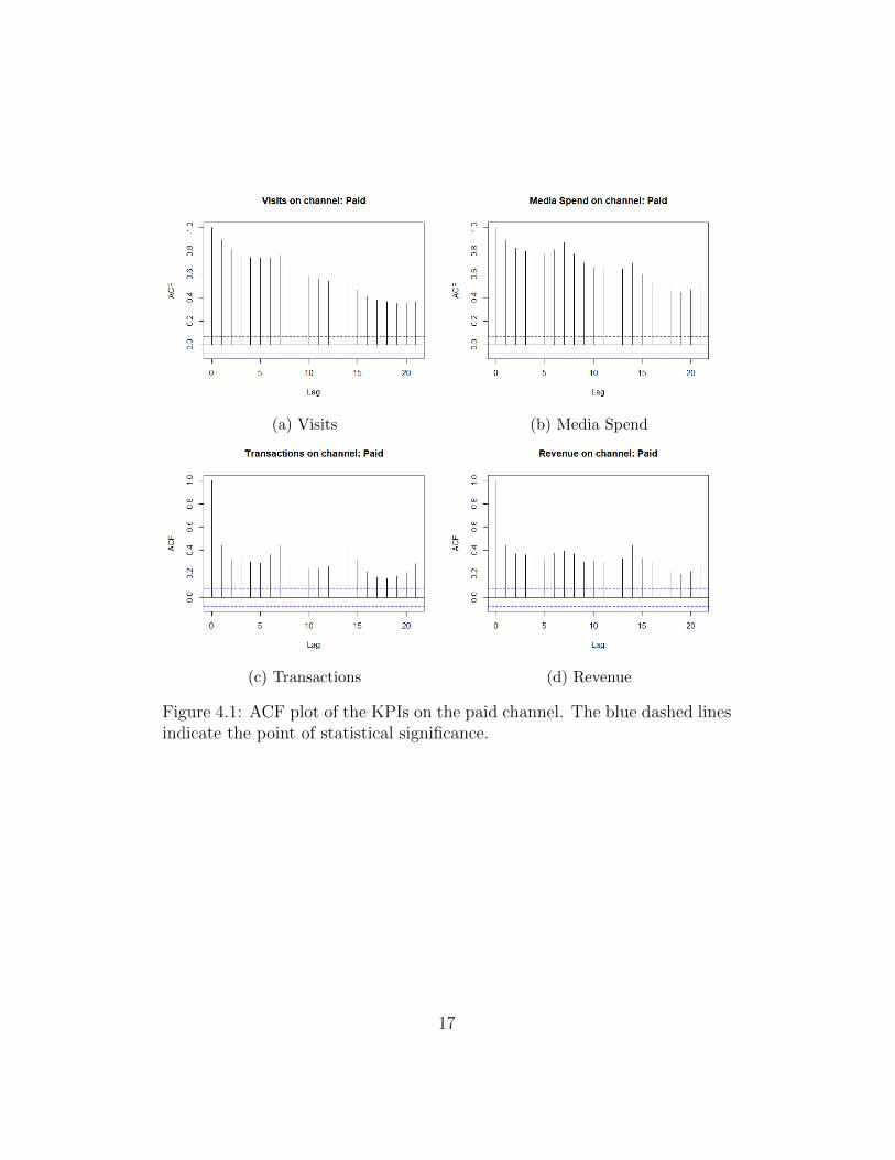
(a) Visits (b) Media Spend
(c) Transactions (d) Revenue
Figure 42 PACF plot of the KPIs on the paid channel The blue dashedlines indicate the point of statistical significance
We observe that the ACF plot shows a slight peak at every 7th lag for allKPIs This indicates a weekly pattern The PACF plot shows a significantspike at lag 1 for all KPIs This indicates that the KPI value of previousday is very strong correlated with the value of current day For visits andmedia spend the lags 1 to 7 is significantly positive correlated Moreoverlag 8 is negative correlated and lags beyond 8 become less significant Fortransactions and revenue we observe significance until lag 7 followed by aspike at lag 14 that is caused by the weekly pattern
18
The final analysis is the exploration of the statistical relationship between theKPIs and the other metrics in the data The Pearson correlation between thedifferent variables in the data is computed Since we use past observations topredict the KPIs the correlation is between the current day KPIs value andthe metrics value of previous day except for weather inflation and unemploy-ment The values for weather are at the same day because weather forecastcan be derived from other resources This forecast can then be used as pre-dictor for the KPIs The value for inflation and unemployment is from theprevious month because daily observations are not available Even thoughthis is the case it can still help in daily forecast as inflation and unemploy-ment usually have a long term effect The correlation matrix for the paidchannel is shown in a correlogram in Figure 43
Figure 43 Pearson correlation matrix of the data on the paid channel
19
We observe correlations between KPIs themselves Visits (gasessions) ispositive correlated with media spend (gaadCost) which indicates that anincrease in media spend of the previous day results in an increase in next dayvisits Transactions is strong positive correlated with revenue (gatransactionRevenue)which is obvious The current day visits is strong correlated with previousday users and new users This can be explained by the fact that every singleuser generates at least one session Moreover a positive correlation is ob-served between visits and impressions and adClicks which shows the positiverelation between advertising and visits
For media spend we observe a positive correlation with impressions adclicksand number of active campaigns which is natural
With the obtained insights from the data analysis we have a good interpre-tation about which data can be used as features in the models This will befurther described in the experiments in section 62
20
5 Methods and Models
This section describes the models that are used for the forecast the multi-step forecasting method and the evaluation method
51 Models
511 Ratio-based model
The Ratio-based model is used as a benchmark model This model takes thehistorical data of a certain number of weeks before and computes the changein ratios over the same day for every week Next these ratios are averagedinto a single ratio and this single ratio is used as predictor for the next timestep
If we define Xt as the KPI at time step t and we take k weeks as historicaldata then the ratio change for Xt is given by
Ratiot =1
k
ksumi=1
Xt+1minus7i minusXtminus7i
Xtminus7i(51)
However problem occurs when the historical KPIs are zero ie Xtminus7i = 0for i = 1 k This will result in a division of zero which is not possibleTherefore in this case we take the difference of the KPIs instead of the ratio
Differencet =1
k
ksumi=1
Xt+1minus7i minusXtminus7i (52)
Moreover the difference forecast will be applied when Xt is zero as the ratioforecast will always result in a zero Thus the forecast on Xt+1 is given by
Xt+1 =
Xt lowast (1 + Ratiot) if Xt gt 0 or Ratiot is definedXt + Differencet if Xt = 0 or Ratiot is undefined
(53)
21
This equation expresses the single-step forecast The mathematical expres-sion for the recursive multi-step forecast is then
Xt+n =
nminus1prodi=0
(1 + Ratiot+i) lowastXt if Xt gt 0 or Ratiot+i is defined
nminus1sumi=0
Differencet+i +Xt if Xt = 0 or Ratiot+i is undefined
(54)
Notice that the ratio and the difference are always taken on the next timestep ie the ratio and difference between Xt and Xt+1 However we can alsotake the ratio and difference between multiple time steps ie between Xt andXt+n This will avoid the recursive strategy that usually has accumulatederror The ratio and the difference are then expressed as
Ratiot+n =1
k
ksumi=1
Xt+nminus7i minusXtminus7i
Xtminus7i
Differencet+n =1
k
ksumi=1
Xt+nminus7i minusXtminus7i
(55)
Next the non-recursive multi-step ahead forecast is given by
Xt+n =
Xt lowast (1 + Ratiot+n) if Xt gt 0 or Ratiot+n is definedXt + Differencet+n if Xt = 0 or Ratiot+n is undefined
(56)
The Ratio-based model for both the recursive and non-recursive multi-stepahead is illustrated in Figure 51
22
(a) Recursive forecast
(b) Non-recursive forecast
Figure 51 The Ratio-based model recursive and non-recursive forecastusing one week historical data The blue observations are the historicalobservations and the red observations are the forecast time steps
The advantage of this model is its simplicity and flexibility The model canbe easily implemented for all the KPIs and it is able to produce a forecasteven when little data is available The disadvantage is the reliability of themodel as large variation in KPIs over the weeks can easily result in inaccurateforecast
512 ARIMA
The ARIMA model is a stochastic time series model that combines threeprocesses the Autoregressive process (AR) the strip off of the integrated (I)time series by differencing and the Moving Averages (MA) [10] In an ARprocess the future value of a variable is assumed to be a linear combinationof p past observations plus a random error and a constant In a MA processthe past observations are the q past errors instead of the past observationsThus it is a linear combination of q past errors plus a random error and themean of the series These two processes can be combined together to forma more effective time series model This model is known as ARMA(pq) [22]and is given by
23
Xt = α1Xtminus1 + + αpXtminusp + εt + β1εtminus1 + + βqεtminusq (57)
where Xt is the observation at time t and εt is the random error at time tThis equation can be written implicitly as
(1minus
psumk=1
αkLk)Xt =
(1 +
qsumk=1
βkLk)εt (58)
where p and q are the order of the autoregressive and moving average partsof the model respectively and L is the lag operator
However ARMA can only be used for stationary time series ie the meanand variance of the time series do not depend upon time This is not the casein many time series such as in economic time series that contain trends andseasonal patterns Therefore the integrated term is introduced to include thecases of non-stationarity by applying differencing The difference operatortakes a differencing of order d and it is expressed as follows
∆dXt = (1minus L)dXt (59)
where Xt is the data point at time t L is the lag operator and d is the orderThus the three processes AR(p) I(d) and MA(q) are combined interactedand recomposed into the ARIMA(p d q) model
The general method to identify the order p in an AR process and q in aMA process is to use the autocorrelation function (ACF) and the partialautocorrelation function (PACF) [21] For a pure AR(p) process the PACFcuts down to zero after lag p For a pure MA(q) process the ACF cuts downto zero after lag q For ARMA(p q) and ARIMA(p d q) processes it is morecomplicated to estimate the parameters A method to do this is to performa grid search over these parameters using an evaluation metric for modelselection
24
513 Random Forest
Random Forest is a machine learning model for classification and regression[23] and it is illustrated in Figure 52
Figure 52 Random Forest [24]
Random Forest is an ensemble learning method that combines a group ofweak learners to form a more powerful model These weak learners are deci-sion trees and they can either be used for classification or regression In ourcase the focus is on regression
A decision tree is made up of decisions nodes terminal nodes (leaves) andbranches These branches represent the possible paths from one node toanother Decision trees are recursive partitioning algorithm that split thedataset in smaller subsets using a top-down greedy approach It starts atthe root node (top decision node) where a certain feature variable is usedto split the data into subsets Because the dataset can be split in numerousways the feature variable and its split point that yields the largest reductionin the residuals sum of squares (RSS) is chosen
Nsumn=1
sumiisinRn
(yi minus yn)2 (510)
where yi is the training observation i and yn is the mean of the responsevalues for the training observation that fall into the subset n
25
Next the decision tree recursively splits the dataset from the root nodeonwards at each decision node until the terminal nodes These terminalnodes are the endpoints of the decision tree and represent the final result ofa combination of decisions and events They are reached when all recordsafter the split belong to the same target variable or until a stopping criterionis met
In Random Forest a large number of these decision trees are constructed andeach tree makes a random selection of independent variables This results invariance in predictions between various decision trees which reduce overfittingand variance Then the prediction is produced by taking the mean predictionof the individual trees
Besides the number of trees in the forest it has other parameters that canbe varied such as the maximum depth of the tree the minimum number ofsamples required to split a decision node the minimum number of samplesrequired to be at a leaf node and the number of features to consider whenlooking for the best split
514 Artificial Neural Networks
ANNs are inspired by biological systems and the human brain and they haveshown powerful pattern classification and recognition capabilities [11] ANNslearn from experience by recognizing patterns in the input data Next theymake predictions based on their prior knowledge ANNs are applied in manydifferent fields of industry business and science [25] There are differenttypes of ANNs we have applied the feed-forward neural network (FNN) andthe recurrent neural network (RNN) [26 27] The FNN is the Multi-LayerPerceptron and the RNN is the Long Short-Term Memory
5141 Multi-Layer Perceptron
The Multi-Layer Perceptron (MLP) is a class of FNN Figure 53 illustratesthe architecture of a MLP
26
Figure 53 Architecture of a MLP with 3 layers (input hidden and output)with 4 input neurons 5 hidden neurons and 1 output neuron [28] Noticethat MLP can have multiple hidden layers
The network consists of processing elements also known as neurons that areorganized in layers Every neuron in a layer is connected with all the neuronsin the previous layers by acyclic links each with an associated weight Theseweights encode the knowledge of a network The neurons in the layers areused for transformation from input to output The output of each neuron yin the hidden layer(s) and output layer is a (non) linear function over the dotproduct of the weights of the connections with the outputs of the neurons inthe previous layer
y = φ
(sumi
ωixi + b
)(511)
Here xi are the inputs of the neuron ωi are the weights of the neuron and bis the bias φ is the activation function that determines the activation levelof the neuron
During training of the network the weights are modified such that the dif-ference between the network output and the actual output are minimized
27
Thus the estimation of the weights are based on the minimization of thecost function In our model this cost function is the mean squared errorIn order for the network to know how to adjust the weights it uses learningalgorithms The traditional learning algorithm is backpropagation [29] andit works as follows
1 Compute the feed-forward signals from the input to the output
2 Compute the error E of each neuron of the output layer using the costfunction
3 Backpropagate the error by the gradients of the associated activationfunctions and weighting it by the weights in previous layers
4 Compute the gradients for the set of parameters based on the feed-forward signals and the backpropagated error
5 Update the parameters using the computed gradients
∆ωij = αδjyi where (512)
δj =
φprime(vj)(tj minus yj) if j is an output nodeφprime(vj)
sumk of next layer δkωjk if j is an hidden node
Here ωij is the weight between node i and node j α is the learningrate yj is the output of node j vj is the activation of node j and tj isthe target output of node j
Even though backpropagation is used to solve many practical problems itshows problems such as slow convergence and getting stuck at local minima[29] Therefore other learning algorithms have been developed to improvethe performance of the backpropagation algorithm One of these learningalgorithms is the Adaptive Moment Estimation (Adam) [30] Adam is astochastic gradient descent algorithm based on estimation of first and secondorder moments of the gradients The algorithm works as follows
1 Compute the gradient using the current parameters
2 Update biased first order and second order moments estimate
mt = β1mtminus1 + (1minus β1)gtvt = β2vtminus1 + (1minus β2)g2t
(513)
28
Here mt is first order moment at time step t vt is the second ordermoment at time step t gt is the gradient at time step t and g2t indicatesthe element-wise square of gt β1 and β2 are the exponential decay ratesbetween 0 and 1
3 Compute the bias-corrected first and second order moments
mt =mt
1minus βt1
vt =vt
1minus βt2
(514)
4 Compute weight update and update parameters
θt = θtminus1 minus αmt
(radicvt + ε)
(515)
Here θt is the parameter vector at time step t and α is the learningrate
Adam computes adaptive learning rates for each parameter [31] that speedsup the learning phase This leads to faster convergence Furthermore littlemanual tuning of hyperparameters are required because they have intuitiveinterpretation All these advantages are beneficial for all the models thatneed to be constructed Therefore Adam is used as learning algorithm
5142 Long Short-Term Memory
In FNNs information is only propagated in one direction This is in contrastto recurrent neural networks (RNNs) where information is propagated in bi-directions using feedback loops These feedback loops transfer internal andoutput signals back to the input level which allows information to persistThus a RNN has an internal memory that captures information about whathas been calculated so far This becomes clear if we unfold the RNN throughtime as shown in Figure 54
29
Figure 54 A RNN unfolded in time [32] Here U V W represent the set ofweights xt is the input at time step t st is the hidden state at time step tand ot is the output at time step t
Therefore RNNs can model temporal dependencies of unspecified durationbetween the inputs and the associated desired outputs [33] Because of thisRNNs are suitable for time series predictions However when the gap be-tween the relevant information and the prediction becomes larger regularRNNs become unable to learn to connect the information because of thevanishing gradients (ie the gradient gets so small that learning either be-comes very slow or stops) The problem of vanishing gradients can be avoidedusing Long Short-Term Memory (LSTM)
LSTM is a specific RNN that is capable of learning long-term dependenciesand it was introduced by Hochreiter and Schmidhuber [34] The networktakes three inputs The input Xt of the current time step t the output fromthe previous LSTM unit htminus1 and the memory of the previous unit Ctminus1
The LSTM unit contains special units called memory blocks in the recurrenthidden layer An individual memory block is shown in Figure 55 Eachmemory block contains memory cells and three gated cells that is shared byall the memory cells These three gates are the forget input and output gateand control the information flow to the cells The forget gate decides whatinformation will be removed in the memory The input gate decides whatinformation will be updated The output gate defines what information insidethe cells will be exposed to the external network These gates are controlledby a simple one layer neural network using the sigmoid activation functionThus the network outputs a value between 0 and 1 where 0 represents closed
30
gates and 1 represents open gates
Figure 55 A single LSTM memory block [35]
The forget and input gate use the three LSTM network inputs Xt htminus1 andCtminus1 and a bias vector as input The output gate uses the htminus1 Xt the newmemory Ct and a bias vector as input Thus the forget gate ft input gateit and output gate ot of the current time step t is given by the followingequations
ft = σ(bf +WxfXt +Whfhtminus1 +WcfCtminus1)
it = σ(bi +WxiXt +Whihtminus1 +WciCtminus1)
ot = σ(bo +WxoXt +Whohtminus1 +WcoCt)
(516)
Here σ is the sigmoid function b is the bias vector and W represents the setof weights
The new memory Ct is also generated by a simple neural network but it usesthe hyperbolic tangent as activation function instead of the sigmoid functionThe new memory Ct is then generated by element-wise multiplication of theinput gate it and by adding the old memory Ctminus1
31
Ct = ftCtminus1 + it tanh(bc +WxcXt +Whchtminus1) (517)
Here tanh is the hyperbolic tangent function b is the bias vector and Wrepresents the set of weights
The output ht for the LSTM unit is then generated using the new memoryCt that is controlled by the output gate ot
ht = ot tanh(Ct) (518)
Again the weights in the network need to be learned The learning algorithmAdam is used for this purpose because it can handle the complex training dy-namics of RNNs better than plain gradient descent [30] Moreover since thenetwork uses the hyperbolic tangent function as activation function whichis bounded between -1 and 1 the data is normalized between -1 and 1
52 Multi-step Forecasting Strategies
Since FasterIntel always shows predictions of the KPIs up to Sunday (endof the week) for each week it means that it requires a maximum of 7 daysahead forecast Therefore we decided to forecast the KPIs always 7 timesteps ahead on each day Predicting multiple time steps into the future isalso known as multi-step time series forecasting Different strategies are usedfor multi-step time series forecasting [36] The most common strategies arethe direct multi-step forecast and the recursive multi-step forecast The di-rect multi-step forecast uses a separate model for each forecast time stepwhile the recursive multi-step forecast uses a one-step model multiple timesIt takes the prediction for the prior time step as an input for making a pre-diction on the following time step A disadvantage of the recursive strategyis the accumulation of the prediction errors as the forecast horizon increaseswhile this does not hold in the direct strategy However this does not meanthat the direct strategy is always better than the recursive strategy It alldepends on the model specification Another disadvantage of the recursivestrategy are the unknown values for other time series when they are usedas predictors This means that each time series need to be predicted Thedisadvantage of the direct strategy is that it involves a heavier computationalload than the recursive strategy Moreover since the direct strategy forecasts
32
each time step in isolation of the other time steps it can produce completelyunrelated forecasts over the whole forecast horizon This can lead to un-realistic discontinuities whereas time series have some aspect of continuousbehavior in reality [37] Therefore the recursive strategy is applied in thisresearch
53 Evaluation
The performance of the models is evaluated using the time series cross vali-dation This process is illustrated in Figure 56
Figure 56 The series of training and test sets in time series cross validationThe blue observations form the training sets and the red observations formthe test sets [38]
This validation has a series of training and test sets Each of the test setsconsists of n observations that corresponds with the n time step ahead fore-cast The corresponding training set consists of features that occurred priorto the first observation of the test set This mimics the real-world scenariowhere new observations become available for each time step t Next thisvalidation method walks each series of the test sets one at a time and makesn predictions for each time step
Next the real observations and the predictions for each time step are com-pared with each other using an error measurement The error measurementthat is used is the Root Mean Squared Error (RMSE) and it is given by
33
RMSE =
radicradicradicradic 1
m
msumi=1
(yi minus yi)2 (519)
Here yi is the predicted value for observation i yi is the actual value forobservation i and m is the total number of observations
The RMSE penalizes extreme errors as it is much affected by large individualerrors Thus we obtain n RMSE values where each of these values representsthe error for a single time step t t+ 1 t+ n
34
6 Experimental Setup
This section describes the training and testing of the models the two exper-iments that are conducted and the optimization of the model hyperparame-ters
61 Training and Testing
Since the KPIs have seasonality within a year as shown in the analysis insection 44 it is important that the models are evaluated on at least one yeartest data to capture their overall performance Therefore we chose the last365 days of the dataset as test set starting from 25 May 2016 Notice thatit does not start from 31 May 2016 because observations after 31 May 2017are not available in the dataset when performing 7 days ahead forecast
The models are retrained after each 30 series This corresponds with retrain-ing the model every month The decision to not retrain the models every dayis because retraining on one new observation in the training set will hardlymake any difference in terms of performance
62 Experiments
In this research two experiments have been conducted These experimentsare categorized into experiment A and experiment B
621 Experiment A
In experiment A the data used for each KPI forecast are the correspondinghistorical KPI data along with time related data The time related data arethe month week weekday season and holiday The choice of performing thisexperiment is because the current forecast model only uses the correspondinghistorical KPI data Thus it is interesting for FasterIntel to know about thepredictive performance of each model using only this data The time relateddata is used to capture temporal information from the time series for RandomForest and MLP because they are non-temporal models This is in contrast
35
with ARIMA and LSTM which are temporal models that should be able tocatch temporal information automatically from the time series Thus theinput data for ARIMA and LSTM are only the lagged values of the KPIunder investigation whereas Random Forest and MLP added additional timerelated data and the weekly moving average of the KPI as input to spot theweekly trend
The total number of lags to consider in each model are determined in differentways depending on the model In ARIMA the number of lags is the orderp in the AR part and q in the MA part This order is determined using agrid search method on the validation set that will be described in section63 In LSTM a lag of one is used because information of the lags are passedthrough each recurrent state to the next state In Random Forest and MLPthe number of lags are based on the PACF analysis in section 44 For visitsand media spend the first 8 lags are used and for transactions and revenuethe first 7 lags and the 14th lag are used
Random Forest and ANNs are run for multiple times and the average perfor-mance was taken as final performance for the models This is because thesemodels are stochastic and therefore they return different results on differentruns of the same algorithm on the same data
622 Experiment B
In experiment B all the data are used in the KPIs forecast With this ex-periment we are able to show the difference in performance compared toexperiment A when more data is added This could be interesting for Fas-terIntel as they can set up new businesses with their clients eg offeringbetter KPIs predictive performance for only premium clients However weonly forecast one step ahead instead of multi-step ahead because it becomescomputationally too intensive when additional time series features are addedThe reason is that the recursive strategy requires predictions for every addi-tional time series feature and developing models to do so was out of scopein this thesis Notice that ARIMA is excluded in this experiment as it is aunivariate time series model
In order to ensure that the difference in performance is caused by addingadditional features the same features in experiment A plus the additional
36
features are used These additional features are chosen based on the analysisof the Pearson correlation matrix as shown in Figure 43 The additionalfeatures for the KPIs are shown in Table 61
KPI Additional Features
Visits rdquoad costrdquo rdquousersrdquo rdquonew usersrdquo rdquoimpressionrdquordquoinflationrdquo rdquounemploymentrdquo
Transactions rdquoad costrdquo rdquousersrdquo rdquonew usersrdquo rdquoimpressionrdquordquoaverage temperaturerdquo rdquomaximum temperaturerdquordquoinflationrdquo rdquounemploymentrdquo
Revenue rdquoad costrdquo rdquousersrdquo rdquonew usersrdquo rdquoimpressionrdquordquoaverage temperaturerdquo rdquomaximum temperaturerdquordquoinflationrdquo rdquounemploymentrdquo
Media Spend rdquoimpressionrdquo rdquocampaignsrdquo rdquoad clicksrdquo
Table 61 KPI and its additional features
Again the number of lags for each feature had to be determined in the inputdata as in experiment A Zero lag is chosen for the temperature data as yourcurrent behaviour can be influenced by the current weather condition Alag of one is chosen for the other additional features because it is the mostrepresentative for the current time step Moreover the moving average of 7days for all Google Analytics features and the weather is included which giveinformation about the weekly trend of each time series feature
63 Hyperparameters Optimization
ARIMA Random Forest MLP and LSTM all have hyperparameters thatneed to be optimized to achieve good performance The hyperparametersin ARIMA are the auto regressive order p the integration order d and themoving average order q For Random Forest MLP and LSTM not all hyper-parameters are considered The ones that are considered in Random Forestare the number of trees in the forest the number of features to consider whenlooking for the best split and the minimum sample leaf size The hyperpa-rameters that are considered in MLP are the number of hidden layers andneurons in each layer and the activation functions The hyperparameters
37
that are considered in LSTM are the number of hidden layers and LSTMunits in each layer
All the combinations of the hyperparameters were tested on the validationset This validation set is a separation of the first training set in the timeseries cross validation and contains one month of data starting from 25 April2016 to 24 May 2016 Thus the models were trained on the data before 25April 2016 Next each model was trained again on the whole first trainingset using the optimal hyperparameters and evaluated using time series crossvalidation as described in section 53
The hyperparameter optimization for ARIMA was performed using a gridsearch method This method tries every hyperparameter setting over a spec-ified range of values The search range for the autoregressive order p andmoving average order q was set based on the PACF and ACF analysis insection 44 respectively For the autoregressive order p it was set from 0 to8 for visits and media spend and from 0 to 14 for transactions and revenueFor the moving average order q it was set from 0 to 7 for all the KPIs Thesearch range for the integration order d was set from 0 to 1 The choice fora maximum of first order differencing is because second order differencing israrely needed to achieve stationarity [10]
In Random Forest the optimal number of trees was determined to be inthe range from 10 to 400 and the optimal minimum sample leaf size wasdetermined to be in the range from 1 to 50
In MLP the optimal hidden neurons in each hidden layer was determined inthe range 10 to 100 The number of hidden layers was set to a maximum oftwo layers The rectified linear unit (ReLU) activation function was used inthe hidden layers because it was found to be the most efficient when appliedto the forecasting of non-stationary and noisy time series Next the linearactivation function was used in the output layer to output the forecast valueof the time series
In LSTM the number of hidden layers was set to one and the number ofLSTM units was determined in the range 10 to 40 The exponential decayrates β1 and β2 were set to default values of 09 and 0999 respectively Thesedefault values are proposed in the original paper [34]
38
7 Results
In this section the results of the two experiments are presented First section71 presents the results for experiment A and it contains results with regardsto model hyperparameters model performance model comparison and fea-ture importance Next section 72 presents the results for experiment Band it contains results with regards to model hyperparameters model per-formance and feature importance Finally section 73 summarizes the resultsof both experiments
71 Experiment A
711 Hyperparameters
The results for the hyperparameters for ARIMA Random Forest and MLPare shown below
39
ARIMA
Figure 71 ARIMA Order(p d q)2
Figure 71 shows the RMSE for different combinations of order(p d q) Weobserve many fluctuations in errors for the different combinations The op-timal order achieved for visits transactions revenue and media spend is(605) (202) (402) and (706) respectively
2The order(p d q) starts at (000) and is first incremented for q next for d and as lastfor p
40
Random Forest
Figure 72 Random Forest Number Of Trees
Figure 72 shows the RMSE for different number of trees We observe thatthe optimal number of trees for visits is 270 as increasing the number oftrees will not significantly decrease the RMSE anymore For transactionsthe RMSE becomes stable after 120 trees The number of trees that is chosenfor revenue and media spend is 300 and 370 respectively It is not necessaryto increase the number of trees further as the performance stays roughly thesame while the computational time will increase
The optimal maximum number of features to look for the best split wasfound to be the square root of the number of input features The optimalminimum sample leaf size in experiment A was 7 2 3 and 2 for visitstransactions revenue and media spend respectively In experiment B theoptimal minimum sample leaf size was 4 1 4 and 1 for visits transactionsrevenue and media spend respectively
41
MLP
Figure 73 MLP number of hidden layers and hidden neurons
Figure 73 shows the RMSE for different number of hidden layers and hiddenneurons in the training and validation set We observe that the error of thetraining set in visits transactions and revenue is larger than the error inthe validation set This is caused by the different cases in both sets Thetime series in the training set contains data over multiple months whereasthe time series in the validation set contains only data over one month Theseasonality over the different months causes that some months are harder tolearn than other months
We observe a linear decrease in the error of the training set when two hiddenlayers are applied for visits However this is not observed in the validationset The errors are rather stable over the different number of hidden layersand neurons The lowest error is achieved using two hidden layers with 10
42
neurons in each layer For media spend and revenue the use of two hiddenlayers is also sufficient both errors in the training set and validation setdecrease when the number of neurons is increased The error becomes almostconstant after 70 neurons in both layers for media spend and after 60 neuronsin both layers for revenue The lowest error in the validation set is achievedusing two hidden layers with 100 neurons in each layer for media spend andtwo hidden layers with 90 neurons in each layer for revenue For transactionsone hidden layer with 20 neurons gives the smallest error in the validationset
43
LSTM
Figure 74 LSTM number of units
Figure 74 shows the RMSE for different number of LSTM units on thetraining and validation set We observe again that the training set error islarger than the validation error Moreover increasing the number of LSTMunits does not really improve the training set error whereas the validationerror for some KPIs increases The validation error increases after 20 LSTMunit for visits and media spend The validation error for transactions andrevenue are relatively stable for different number of LSTM units The lowesterror is achieved using 10 LSTM unit for transactions and 20 LSTM unit forrevenue
44
712 Model Performance
The performance of each model using the time series cross validation on thepaid channel over 10 runs is shown in Figure 75
Figure 75 Model performance on the paid channel
The Ratio-based model is excluded in transactions and revenue because theerror is off the scale that made the other models not comparable anymoreThe exact values of the RMSE is also shown in tables in Appendix B
We observe that ARIMA MLP and Random Forest outperform the linearregression model (current model) for the four KPIs ARIMA and RandomForest both perform well for visits However MLP starts to perform betterthan ARIMA and Random Forest after time step t+ 4 For media spend weobserved the opposite where MLP performs better until time step t+ 3 andgets bypassed by Random Forest after time step t+3 Random Forest showsthe best performance for transactions and MLP shows the best performancefor revenue The Ratio-based model has the worst performance of all themodels and LSTM performed the worst when comparing to ARIMA MLPand Random Forest These results will be discussed in the discussion insection 8
713 Feature Importance
After training the Random Forest we can obtain their feature importanceand this is shown in Figure 76 for the paid channel
45
Figure 76 Feature Importance of Random Forest on the paid channel
We observe that for visits and media spend the most important feature istminus 1 (lag 1) This means that previous day value is important in predictingthe value on the next day Moreover the moving average shows importancein all the KPIs that give information about trends or cycles Interestingto observe is that lag 8 (t minus 8) shows little importance comparing to theother lags while it shows a strong correlation in the PACF plot in Figure 42Furthermore the model performance is barely affected when lag 8 is removedfrom the model
46
714 Model Comparison
Based on the model performance in Figure 75 we can already compare themodels with each other However to ensure that these model performanceresults are statistically significant the squared errors of the models are testedusing the two-sided Kolmogorov-Smirnov test (K-S test) The two-sidedK-S test is used to test whether two independent samples are drawn fromthe same continuous distribution In our case we are testing whether thesquared errors per instance of two different models are drawn from the samecontinuous distribution This is also known as the KS Predictive Accuracy(KSPA) test [39] Thus we test the null hypothesis
H0 The squared error of model A and model B
come from the same continuous distribution
against the alternative hypothesis
H1 The squared error of model A and model B
do not come from the same continuous distribution
The test is performed for all the forecast horizon However the result fortime step t is only shown here for clarity For visits we obtained the followingp-values between the different models as shown in Table 71
p-value Linear RatioRec
RatioNonRec
ARIMA RandomForest
MLP LSTM
Linear 1 157e-24 157e-24 149e-21 125e-26 123e-15 454e-19RatioRec
157e-24 1 1 216e-05 326e-05 307e-05 132e-09
RatioNonRec
157e-24 1 1 216e-05 326e-05 307e-05 132e-09
ARIMA 149e-21 216e-05 216e-05 1 186e-03 019 321e-03RandomForest
125e-26 326e-05 326e-05 186e-03 1 543e-03 140e-08
MLP 123e-15 307e-05 307e-05 019 543e-03 1 543e-03LSTM 454e-19 132e-09 132e-09 321e-03 140e-08 543e-03 1
Table 71 The p-values from the KSPA test between the models for the KPIvisits for time step t
47
If we assume a significance level of 95 (p-value less than 005) we observethat most of the p-values are significant The only insignificant one is thedistribution of the squared errors between ARIMA and MLP with a p-valueof 019 This means that we cannot reject the null hypothesis and the squarederrors are likely to come from the same distribution This is unexpected asthe RMSE for ARIMA is much lower than MLP as observed in Figure 75Further analysis we found that the empirical distribution of the squarederrors of ARIMA and MLP look almost the same but that MLP contains afew much larger errors than ARIMA This caused the larger RMSE for MLPNext the same analysis is performed for transactions and the result is shownin Table 72
p-value Linear ARIMA RandomForest
MLP LSTM
Linear 1 069 050 045 013ARIMA 069 1 099 099 098RandomForest
050 099 1 1 099
MLP 045 099 1 1 098LSTM 013 098 099 098 1
Table 72 The p-values from the KSPA test between the models for the KPItransactions for time step t
We observe that none of the p-values are significant This indicates thatthe errors for all the models come from the same distribution From theRMSE as shown in Figure 75 we already observe that the difference betweenthese models are very small This difference is mostly caused by the severallarge transactions in the testset where Random Forest predicts these largetransactions the closest
The p-values for revenue are also insignificant for all the models as shownin Table 73 The difference in RSME is also caused by the outliers in thetestset where MLP predicts these the closest
48
p-value Linear ARIMA RandomForest
MLP LSTM
Linear 1 056 022 022 022ARIMA 056 1 030 016 045RandomForest
022 030 1 063 091
MLP 022 016 063 1 030LSTM 022 045 091 030 1
Table 73 The p-values from the KSPA test between the models for the KPIrevenue for time step t
Table 74 shows the p-values between the models for the media spend Weobserve that most of them are significant and the insignificant ones are theerrors between Random Forest and MLP Random Forest and ARIMA andMLP and ARIMA with p-values 063 063 and 045 respectively Moreoverthe difference in RMSE between these models is small as shown in Figure75 Thus it is expected that these squared errors come from the samedistribution
p-value Linear RatioRec
RatioNonRec
ARIMA RandomForest
MLP LSTM
Linear 1 125e-26 125e-26 350e-29 620e-30 119e-34 658e-16RatioRec
125e-26 1 1 001 004 001 556e-09
RatioNonRec
125e-26 1 1 001 004 001 556e-09
ARIMA 350e-29 001 001 1 063 045 129e-07RandomForest
620e-30 004 004 063 1 063 347e-09
MLP 119e-34 001 001 045 063 1 198e-07LSTM 658e-16 556e-09 556e-09 129e-07 347e-09 198e-07 1
Table 74 The p-values from the KSPA test between the models for the KPImedia spend for time step t
When the KSPA test was applied for the other forecast horizons We found
49
for visits that the forecast generated by ARIMA and MLP are not statisticallydifferent from each other for all time steps Moreover the squared errorbetween Random Forest and MLP and the squared error between RandomForest and ARIMA become insignificant after time step t with p-value of010 and 06 respectively This mean that there is no significant differencebetween these three models after time step t
For transactions we found that neither of the models are statistically sig-nificant different from each other for all the forecast horizon This meansthat all models are suitable for forecasting transactions The reason is thatthe variance of transactions is relatively small which makes the forecast errorrelatively similar for all models
For revenue we also found that neither of the models are statistically sig-nificant different from each other for all the forecast horizon This whilewe observe a significant difference in RMSE between some models over theforecast horizon The difference is caused by large revenues that is bettercaptured by some models
For media spend we found that the forecast error between ARIMA andRandom Forest becomes statistically significant after time step t+4 (p-valueof 004) Random Forest is then performing statistically better than ARIMAFurthermore the forecast error of MLP and Random Forest are insignificantfor all time steps which means that they are both performing the same
50
72 Experiment B
721 Hyperparameters
The hyperparameters need to be optimized as in experiment A The samenumber of trees was used as in experiment A because the same behaviour wasobserved in experiment B However this same behaviour was not observedfor the number of neurons in the neural networks In this experiment moreneurons were needed in the neural networks because of the increased numberof inputs The change of the number of neurons in MLP is shown in Table75 and the change of number of LSTM units is shown in Table 76
MLP Experiment A Experiment B
Visits 1010 2020Transactions 20 40Revenue 9090 100100Media Spend 100100 100100
Table 75 The optimal neurons in the hidden layers for experiment A and B
LSTM Experiment A Experiment B
Visits 20 20Transactions 10 40Revenue 10 30Media Spend 20 40
Table 76 The optimal LSTM units for experiment A and B
722 Model Performance
The performance of the models are obtained over 10 runs and the resultalong with the result from experiment A are presented Table 77 shows theRMSE for Random Forest in both experiments and its p-value of the KSPAtest between the squared error of the model in the two experiments
51
Table 77 The RMSE of time step t on the paid channel using RandomForest of experiment A and B and its p-value of the KSPA test
We observe that the RMSE in experiment B does not differ significantly fromthe RMSE in experiment A for all KPIs This is also confirmed by the KSPAtest as non of the p-values are significant Thus the additional features arenot contributing in improving the performance The reason is that theseadditional features are largely irrelevant that will be shown in the featureimportance in Figure 77
Next the result for MLP is shown in Table 78
Table 78 The RMSE of time step t on the paid channel using MLP ofexperiment A and B and its p-value of the KSPA test
The same result as in Random Forest is observed here The performance isnot improving and it is almost the same as experiment A This behaviour isalso observed in LSTM as shown in Table 79 From the results it becomesclear that it has no benefit to add the additional features as the performanceis not improving
Table 79 The RMSE of time step t on the paid channel using LSTM ofexperiment A and B and its p-value of the KSPA test
723 Feature Importance
The feature importance for Random Forest can again be derived to obtainthe importance of the additional features The result is shown in Figure 77
52
Figure 77 Feature Importance of Random Forest including additional fea-tures on the paid channel
We observe for visits that the features rdquousersrdquo and rdquonew usersrdquo are quiteimportant because they have a very strong correlation with visits as shownin Figure 43 rdquoAd costrdquo and rdquoimpressionrdquo on the contrary shows little im-portance
The most important features in media spend are still the same features inexperiment A The additional features rdquoimpressionrdquo rdquoad clicksrdquo and rdquocam-paignsrdquo show little importance
The moving average is still the top important feature in transactions and
53
revenue The additional features seem to have an importance but they areall below 008 which indicates a very low importance
73 Summary
From the results of both experiments we obtained that adding the additionalfeatures in experiment B did not result in improvement Moreover when westatistically compared the performance of the models using the KSPA testsome of the models were insignificant while there was a significant differencein RMSE Further analysis we found out that this difference was caused bysome outliers in the testset Some of the models predicted these outliersbetter than others The model with the lowest error for each KPI performedbetter than the current model The best model for each KPI along with itsaverage improvement over the time steps on the paid channel is shown inTable 710
KPI Best Model Improvement
Visits Random Forest 4175Transactions Random Forest 1704Revenue MLP 1702Media Spend MLP 5600
Table 710 The best models for each KPI on the paid channel and theirimprovement with respect to the current model
Transactions and revenue have the smallest improvement because these arethe hardest to predict The media spend has the greatest improvement How-ever the RMSE of these best models are still large when they are comparedto the magnitude of the values in the test set
54
8 Discussion and Conclusion
The implemented models except the Ratio-based model were able to improvethe forecast of the current model The Ratio-based model resulted in hugeerrors as the variability between the same days over the weeks are large Eventhough improvement is made the performance is still not outstanding Theproblem is not caused by the implemented models but the limited amountof historical data and features available We only have data for three yearswhere one year was already used for testing Thus training on two years ofhistorical data is just too small for the models to learn and understand thedata This especially holds for complex models like neural networks wheremore training data are needed for them to generalize This may explain thebad performance of LSTM whereas ARIMA and Random Forest require lessdata to generalize Moreover the validation set consists of only one monthdata instead of one year that could give the wrong optimal hyperparametersHowever if one year of data is taken as validation set then only one yearof data remains for the training set This is inadequate for training a goodmodel as the yearly patterns cannot be captured Besides the limited datathe recursive strategy can play a role in the performance of the multi-stepahead forecast From the results we have observed that the error increasesalong with the time horizon This error might be reduced when using thedirect strategy
From experiment A we obtained that it is hard to make accurate predictionsof the KPIs based on only their own past values Therefore we includedexternal data that is still applicable for all clients and other Google Analyticsfeatures in experiment B However they have shown less predictive valueMoreover the external data was coarse grained except for weather whichmakes it less valuable for daily forecast Based on the feature importancethe moving average has shown to be always on the top 3 most importantfeature because it captures the overall trend of the KPIs over the time stepsHowever neither of the most important feature exceeded an importance valueof 025 This indicates that the data have low predictive value and other dataare needed
Data that could improve the performance is internal company data How-ever these data cannot be derived from Google Analytics Data such asinformation about the products they offer Relevant information such as
55
the price rating reviews and discounts This information could help in theprediction of transactions and revenue as shown in the literature reviewMoreover information about their upcoming media strategy can be relevant[40] This will all have an impact on the performance of the KPIs Besidesonline marketing offline marketing is also used to increase awareness suchas informative pamphlets flyers television and radio advertising and mag-azines [41] In conclusion internal company data might be important asthey describe the behaviour of KPIs more explicitly However this suggeststhat we have to acquire these data that is not generic anymore and does notmatch with the product point of view Thus there is a trade off betweenperformance and scalability High performance can be acquired when moreattention is paid on each client [42] However this will result in higher costand more time from the business side
Based on this research we would recommend to be cautious with using onlyGoogle Analytics data to forecast the KPIs because limited knowledge canbe gained from this Moreover it is dangerous when marketeers rely on thesebad predictions to take actions because this will lead to wrong actions Forfuture research it would be interesting to acquire company internal dataand more history if available This data together with Google Analyticsdata can then be applied and might improve the KPIs prediction furtherFurthermore we have only focused on the paid channel in this research Itmight be also interesting for future research to forecast the KPIs on the otherchannels Channels that are less affected by advertising such as the directchannel might be easier to predict
The formulated research question was rdquoWith how much can the forecastof KPIs be improved compared to the current model using only data that isgeneric enough to be available from all clientsrdquo The findings in this researchshow that the forecast of visits improved with 42 transactions and revenuewith 17 and media spend with 56 However the prediction error is stilllarge for all KPIs The reason is that generic data can only capture genericinformation on the KPIs whereas many other specific factors can affect theseKPIs Therefore it is really difficult to make accurate predictions using onlygeneric information
56
References
[1] Shuojia Guo and Bingjia Shao ldquoQuantitative evaluation of e-commercialWeb sites of foreign trade enterprises in Chongqingrdquo In 1 (June 2005)780ndash785 Vol 1
[2] statista Retail e-commerce sales worldwide from 2014 to 2021 (in bil-lion US dollars) httpswwwstatistacomstatistics379046worldwide-retail-e-commerce-sales
[3] Alanah J Davis and Deepak Khazanchi ldquoAn Empirical Study of OnlineWord of Mouth as a Predictor for Multi-product Category e-CommerceSalesrdquo In 18 (May 2008) pp 130ndash141
[4] C Ranganathan and Elizabeth Grandon ldquoAn Exploratory Examina-tion of Factors Affecting Online Salesrdquo In Journal of Computer Infor-mation Systems 423 (2002) pp 87ndash93
[5] Qiang Ye Rob Law and Bin Gu ldquoThe Impact of Online User Reviewson Hotel Room Salesrdquo In 28 (Mar 2009) pp 180ndash182
[6] James W Taylor ldquoForecasting daily supermarket sales using exponen-tially weighted quantile regressionrdquo In European Journal of Opera-tional Research 1781 (2007) pp 154ndash167
[7] Besta P Lenort R ldquoHierarchical Sales Forecasting System for ApparelCompanies and Supply Chainsrdquo In 21 (2013) pp 7ndash11
[8] Ilan Alon Min Qi and Robert J Sadowski ldquoForecasting aggregateretail sales a comparison of artificial neural networks and traditionalmethodsrdquo In Journal of Retailing and Consumer Services 83 (2001)pp 147ndash156
[9] Gareth James et al An Introduction to Statistical Learning With Ap-plications in R Springer Publishing Company Incorporated 2014
[10] By George E P Box et al Time Series Analysis Forecasting and Con-trol Vol 68 Jan 2016 isbn 978-1-118-67502-1
[11] GPZhang ldquoNeural Networks for Time-Series Forecastingrdquo In Hand-book of Natural Computing (2012) pp 461ndash477
[12] Vincent Cho ldquoA comparison of three different approaches to touristarrival forecastingrdquo In Tourism Management 243 (2003) pp 323ndash330
[13] F M Thiesing and O Vornberger ldquoSales forecasting using neuralnetworksrdquo In Neural Networks1997 International Conference on 4(1997) 2125ndash2128 vol4
57
[14] Peter vd Reijden and Otto Koppius ldquoTHE VALUE OF ONLINEPRODUCT BUZZ IN SALES FORECASTINGrdquo In International Con-ference on Information Systems (2010)
[15] Kris Johnson Ferreira Bin Hong Alex Lee and David Simchi-LevildquoAnalytics for an Online Retailer Demand Forecasting and Price Op-timizationrdquo In Manufacturing amp Service Operations Management 181(2016) pp 69ndash88
[16] P Meulstee and M Pechenizkiy ldquoFood Sales Prediction rdquoIf Only ItKnew What We Knowrdquordquo In 2008 IEEE International Conference onData Mining Workshops (2008) pp 134ndash143
[17] Kyle B Murray et al ldquoThe effect of weather on consumer spendingrdquoIn Journal of Retailing and Consumer Services 176 (2010) pp 512ndash520
[18] Google Analytics Solutions httpswwwgooglecomanalyticsanalyticsmodal_active=none
[19] KlimatologieDaggegevens van het weer in Nederland httpprojectsknminlklimatologiedaggegevensselectiecgi
[20] Centraal Bureau voor de Statistiek StatLine httpstatlinecbsnlStatwebLA=nl
[21] Ratnadip Adhikari and R K Agrawal An Introductory Study on Timeseries Modeling and Forecasting Jan 2013 isbn 978-3-659-33508-2
[22] BChoi ARMA Model Identification Springer Series in Statistics 1992isbn 978-1-4613-9745-8
[23] TK Ho ldquoRandom decision forestsrdquo In In Document Analysis andRecognition (1995) pp 278ndash282
[24] Dan Benyamin A Gentle Introduction to Random Forests Ensemblesand Performance Metrics in a Commercial System httpblog
citizennetcomblog20121110random-forests-ensembles-
and-performance-metrics[25] MA Lehr BWidrow DERumelhart ldquoNeural networks Applications
in industry business and sciencerdquo In Communications of the ACM(1994) pp 93ndash105
[26] Z Tang and PA Fishwick ldquoFeedforward Neural Nets as Models forTime Series Forecastingrdquo In ORSA Journal on Computing (1993)pp 374ndash385
[27] G Dorffner ldquoNeural Networks for Time Series Processingrdquo In 6 (1996)[28] J Cazala Perceptron https github com cazala synaptic
wikiArchitect
58
[29] R Hecht-Nielsen ldquoTheory of the backpropagation neural networkrdquo In(1989) 593ndash605 vol1
[30] PDKingma and JLBa ldquoAdam a method for stochastic optimiza-tionrdquo In ICLR (2015)
[31] Sebastian Ruder ldquoAn overview of gradient descent optimization algo-rithmsrdquo In (Sept 2016)
[32] D Britz Recurrent Neural Networks Tutorial Part 1 ndash Introductionto RNNs httpwwwwildmlcom201509recurrent-neural-networks-tutorial-part-1-introduction-to-rnns
[33] M Assaad and R Bone ldquoA new boosting algorithm for improved time-series forecasting with recurrent neural networksrdquo In Information Fu-sion 91 (2008) pp 41ndash55
[34] Sepp Hochreiter and Jurgen Schmidhuber ldquoLong Short-term Mem-oryrdquo In 9 (Dec 1997) pp 1735ndash80
[35] colah Understanding LSTM Networks httpblogotoronet
20150514long-short-term-memory[36] SB Taieb and RJ Hyndman ldquoRecursive and direct multi-step fore-
casting the best of both worldsrdquo In (2012)[37] S B Taieb and A F Atiya ldquoA Bias and Variance Analysis for Multistep-
Ahead Time Series Forecastingrdquo In IEEE Transactions on Neural Net-works and Learning Systems 271 (Jan 2016) pp 62ndash76
[38] Rob J Hyndman Cross-validation for time series httpsrobjhyndmancomhyndsighttscv
[39] Hossein Hassani and Emmanuel Sirimal Silva ldquoA Kolmogorov-SmirnovBased Test for Comparing the Predictive Accuracy of Two Sets ofForecastsrdquo In Econometrics 33 (2015) pp 590ndash609
[40] Brian Smith ldquoThe effectiveness of marketing strategy making pro-cesses A critical literature review and a research agendardquo In Jour-nal of Targeting Measurement and Analysis for Marketing 113 (Jan2003) pp 273ndash290
[41] Jura Liaukonyte Thales Teixeira and Kenneth C Wilbur ldquoTelevisionAdvertising and Online Shoppingrdquo In Marketing Science 343 (2015)pp 311ndash330
[42] Bob Edmundson Michael Lawrence and Marcus OrsquoConnor ldquoThe useof non-time series information in sales forecasting A case studyrdquo InJournal of Forecasting 73 (1988) pp 201ndash211
59
Appendices
A Additional Results Data Analysis
A1 The KPIs over monthly periods
A2 The KPIs over weekdays
B Model Performance Experiment A
B1 Visits
B2 Transactions
B3 Revenue
B4 Media Spend
60
- Preface
- Abstract
- Introduction
- Background
-
- Company Description
- KPIs and Channels
-
- KPIs
- Channels
-
- Current Model
-
- Literature Review
- Data
-
- Google Analytics Data
- External Data
- Data pre-processing
- Data Analysis
-
- Methods and Models
-
- Models
-
- Ratio-based model
- ARIMA
- Random Forest
- Artificial Neural Networks
-
- Multi-step Forecasting Strategies
- Evaluation
-
- Experimental Setup
-
- Training and Testing
- Experiments
-
- Experiment A
- Experiment B
-
- Hyperparameters Optimization
-
- Results
-
- Experiment A
-
- Hyperparameters
- Model Performance
- Feature Importance
- Model Comparison
-
- Experiment B
-
- Hyperparameters
- Model Performance
- Feature Importance
-
- Summary
-
- Discussion and Conclusion
- References
- Appendices
- Additional Results Data Analysis
-
- The KPIs over monthly periods
- The KPIs over weekdays
-
- Model Performance Experiment A
-
- Visits
- Transactions
- Revenue
- Media Spend
-