forecasting earthquakes and earthquake · pdf fileelsevier international journal of...
TRANSCRIPT
ELSEVIER International Journal of Forecasting 11 (1995) 503-538
Forecasting earthquakes and earthquake risk
David Vere-Jones Institute of Statistics and Operations Research, Victoria University of Wellington, Wellington, New Zealand
Abstract
This paper reviews issues, models, and methodologies arising out of the problems of predicting earthquakes and forecasting earthquake risk. The emphasis is on statistical methods which attempt to quantify the probability of an earthquake occurring within specified time, space, and magnitude windows. One recurring theme is that such probabilities are best developed from models which specify a time-varying conditional intensity (conditional probability per unit time, area or volume, and magnitude interval) for every point in the region under study. The paper comprises three introductory sections, and three substantive sections. The former outline the current state of earthquake prediction, earthquakes and their parameters, and the point process background. The latter cover the estimation of background risk, the estimation of time-varying risk, and some specific examples of models and prediction algorithms. The paper concludes with some brief comments on the links between forecasting earthquakes and other forecasting problems.
Keywords: Earthquake prediction; Seismic hazards; Point process modelling; Conditional intensity models; Probability forecasting
1. Introduction
Natural hazards are assuming ever greater economic importance, not only on a regional but also on a global scale. The growth of major cities in hazard prone areas, and the public anxiety associated with risks to critical facilities such as nuclear reactors, has focused attention on the problems of insurance against natural hazards, disaster mitigation, and disaster prevention.
Within this general area, the earthquake haz- ard stands out as one of the most intractable. While basic knowledge is available about levels of background risk, nothing yet exists for earth- quakes comparable to the warning systems (for
all their defects) currently available in respect of floods, hurricanes, and volcanic eruptions.
Twenty years ago there was considerable op- timism among scientists concerning the future of earthquake prediction. Many observational studies showed that the occurrence of major earthquakes was preceded, at least on some occasions, by anomalous behaviour in a wide variety of physical variables-some less surpris- ing, such as increases or fluctuations in the frequency of smaller events, but others more surprising, such as anomalous fluctuations of magnetic and electric fields, not to mention anomalous animal behaviour. Out of so many possibilities, there seemed a good chance of
0169-2070/95/$09.50 © 1995 Elsevier Science B.V. All rights reserved SSDI 0169-2070(95)0062l-4

504 D. Vere-Jones / International Journal of Forecasting 11 (1995) 503-538
developing reliable precursory indicators which, like rising river levels for flooding, would pro- vide the basis for early warning procedures against earthquakes.
The intervening twenty years have brought a salutary reminder that nature does not reveal her secrets easily. Rikitake (1976) and Mogi (1985) give systematic accounts of the physical phenom- ena which may be associated with earthquake occurrence, and report on a case-by-case basis some Japanese efforts to use such phenomena in developing earthquake predictions; Chinese ef- forts are reported by Ma et al. (1990). A recent and somewhat iconoclastic overview is given by Lomnitz (1994). While it is possible to retain, as the present writer certainly does, some measure of optimism in the long-term outcome of such efforts, three major obstacles have become very apparent. First, the process of earthquake for- mation is complex; as indeed is true of most other forms of fracture. Second, extensive and reliable data on possible precursors of major earthquakes are expensive to collect, and take a long time to accumulate. Third, processes which have their origin some 5, 10 or even 20 km below the earth's surface are singularly resistant to direct observation. Very accurate instruments for measuring changes of level and tilt of the ground have been put in place, but the fluctuations they reveal are not easily related to the occurrence of major events. Changes may appear before some earthquakes but not before others; or they may appear and stabilize without any major event occurring. Much the same can be said about the other proposed predictors. An impression is beginning to emerge that in seismically active areas, large segments of the earth's crust are in some sense close to a critical state; small per- turbations can produce unexpectedly large ef- fects, even at a distance; energy, stored gradual- ly in a volume of the crust, is released sporadi- cally through a complex network of interacting faults, in patterns that have a fractal rather than a regular character.
The growing recognition of these difficulties has highlighted the need to formulate models for earthquake occurrence in probabilistic terms.
Acceptance of this viewpoint has not come easily to the geophysicists, who, in common with many other physical scientists, have a predisposi- tion to view the world in deterministic terms. A notable exception was Sir Harold Jeffreys who warned, more than fifty years ago, that 'A physical law is not an exact prediction, but a statement of the relative probabilities of varia- tions of different amounts; ... the most that the laws do is to predict a variation that accounts for the greater part of the observed variation. The balance is called 'error' and is usually quickly forgotten or altogether disregarded.' (Jeffreys, 1939)
Early exPectations that earthquake predictions could be made deterministically, or with an error which could be "quickly forgotten or altogether disregarded", have proved unfounded. The probabilities have come to take a central role. The distinguished contemporary seismologist, Keiiti Aki, wrote recently that 'I would like to define the task of the physical scientist in earthquake prediction as estimating objectively the probability of occurrence of an earthquake within a specified time, place and time window, under the condition that a particular set of precursory phenomena was observed.' (Aki, 1989)
As early as 1984, a similar sentiment was built into a protocol of UNESCO and IASPEI (the International Association of Seismology and Physics of the Earth's Interior) (IUGG, 1984). It recommends, "that predictions should be formu- lated in terms of probability, i.e. the expectation in the time-space-magnitude domain, of the occurrence of an earthquake". Later, it elabo- rates,
'As prediction develops in the course of con- tinuous monitoring of the region, the expectation may be progressively modified on the basis of further precursory data, or other relevant occur- rences so that the prediction process itself be- comes continuous. Likewise the performance of the hypothesis can be continuously reassessed. The region being monitored will in general include areas of reduced expectation as well as areas of increased expectation, and the proce-
D, Vere-Jones / International Journal of Forecasting 11 (1995) 503-538 505
dure as a whole can, if appropriate, be readily adopted as a basis for designing or modifying earthquake countermeasures in the region.'
Even if deterministic prediction is no longer regarded as a realistic goal, it still casts its shadow over the formulation of prediction and forecasting algorithms. There is often an implicit assumption that the alternative to a deterministic prediction is a deterministic prediction with error. One of the recurrent themes of the pres- ent paper is that even this concession may not be sufficient. Rather, somewhat as in quantum theory, one needs to think of an evolving field of probabilities, within which the concept of "the predicted event" loses any precise meaning. The nearest equivalent to a predicted event is a region with very high concentration of probabili- ty, but even here the patterns are constantly being modified as new predictive information comes to hand.
The protocol quoted earlier goes on to discuss the special responsibilities which devolve upon authors and journal editors intending to publish a paper which incorporates material equivalent to an earthquake prediction. This is a reminder of the difficulty of divorcing the scientific aspects of research in this area from its social, economic, and political implications. The seismologists had their fingers badly burned in this regard in a well-known incident where a scientific journal published a paper forecasting a major earth- quake in the close vicinity of a major city. The local press became aware of this prediction, and drew attention to it, causing some degree of panic. No earthquake in fact occurred, and the scientific basis of the prediction was subsequently discredited, but the incident highlighted the importance of preliminary consultation and scrupulous refereeing before material of this kind is published, even in a scientific journal. For a full account of the event and its implica- tions see Olson et al. (1989).
The incident also highlights a central problem currently facing both scientists and adminis- trators concerned with earthquake prediction: how to proceed in the light of plausible, but not fully statistically substantiated, models or hy-
potheses? To be "fully statistically substan- tiated" means here that the proposed prediction procedure should be backed by a sufficient number of directly observed successes and fail- ures to establish its performance at some agreed level. This is more stringent than having general evidence in favour of the theory or model on which the procedure is based, or extrapolating from small events to large ones, or from a retrospective analysis to a prospective one.
There are analogies with the problems facing the medical profession in regard to the use of a promising new drug which still awaits clinical trialing. The rigorous procedures surrounding clinical trials can be compared to the procedures for testing earthquake prediction algorithms pro- posed in a series of papers by Evison and Rhoades-see, for example, Rhoades and Evison (1979, 1989), Rhoades (1989), Evison and Rhoades (1993). In the clinical trials context, the need for rigorously designed and conducted statistical tests has been found essential to safe- guard the public interest. Evison and Rhoades argue that something similar should be required for prospective schemes of earthquake predic- tion. One difficulty with earthquakes however, is that it could take decades or even centuries to accumulate the information necessary to fully statistically substantiate a proposed method of prediction for great earthquakes. Whether, and under what circumstances, any lower level of verification could be acceptable is one of the key points at issue.
An important recent development has been the decision by the USGS (United States Geological Survey) to publish official assess- ments of the probabilities of damaging earth- quakes affecting different parts of California over specified horizons (see Working Group on Californian Earthquake Probabilities, 1988, 1990). These assessments are intended to repre- sent the best available scientific opinion at the time they are published. However, the basis of their calculations has already been seriously challenged (see Kagan and Jackson, 1991, 1994b). While such challenges may be seen as a necessary and natural part of the evolution of
506 D. Vere-Jones / International Journal of Forecasting 11 (1995) 503-538
improved forecasting methods, they highlight the dangers of basing operational decisions on only partially tested hypotheses.
It seems difficult to argue, however, that such calculations should not be made, and that they should not be made publicly available. The problem is rather in finding the proper adminis- trative response to estimates which are admitted- ly based on provisional hypotheses.
Several authors have recently treated the problem of calling an earthquake alert from a decision-theoretic point of view (see Ellis (1985), Molchan (1991), and the discussion in Section 5 of the present article). They conclude that under quite wide conditions the optimal strategy will have the form "call an alert when the conditional probability intensity [see Section 3 for defini- tions] exceeds a certain threshold level". Such considerations reinforce the view that the pri- mary task of the scientist concerned with earth- quake prediction should be the development of theories and models which allow such condition- al probabilities to be explicitly calculated from past information. On the other hand the de- velopment of an alarm strategy, including the setting of suitable threshold levels and the ac- tions which should follow an alarm, should not be the responsibility of the scientist, but of a group representing appropriate local and nation- al authorities, with the scientist (not to mention the statistician) in an advisory ~ole.
In the sense of a decision to call an earthquake alert, there have been several examples of suc- cessful earthquake predictions, notably in China (see for example, Cao and Aki, 1983). The most famous of these was the Haicheng earthquake of 1975, when the decision to evacuate substantial numbers of people from the city was made less than 24 hours before the occurrence of a major earthquake. Such examples illustrate, from a different point of view, the fact that making an earthquake prediction is a different problem from quantifying the risk. The information avail- able to the Chinese seismologists in Haicheng in 1975 was not very different in kind to what is available to most other seismologists (although the Chinese tend to be more assiduous in collect-
ing and reporting data, and more eclectic in the forms of information they are willing to consider, than their Western colleagues). It appears that the process of quantifying the risk was relatively informal, but took place within a environment that, in this case at least, enabled a bold decision to be taken and acted upon (see Bolt (1988); Lomnitz (1994) takes a more sceptical view of the proceedings).
Decisions to act upon information provided by scientists have been taken in countries other than China. In both Japan and the US, areas have been declared temporary high risk zones where particular precautions should be taken (for ex- ample, Mogi, 1985; Bakun et al., 1986). The overall record of such efforts, however, is not impressive. The form of alert has been rather generalised and, in the cases known to me, the predicted event has failed to materialise. In other cases, major events have occurred without any form of alert being issued.
In summary, it must be admitted that attempts to estimate time-varying risks, or to issue earth- quake predictions, have so far yielded less of practical value than the long-term/static esti- mates of average risk used in engineering and insurance applications. The development of building codes and associated zoning schemes, the use of long-term risk estimates as essential input to the design of risk-sensitive structures, and the development of risk estimates for earth- quake insurance and reinsurance, have contribu- ted substantially to reducing both human and economic losses from earthquakes. Despite their great potential, earthquake prediction methods have still to reach the stage where they make a comparable contribution.
In the remainder of this article I shall look in more detail at some of the statistical models and methods which have been suggested for estimat- ing both static and time-varying risks. The next two sections give a brief summary of the techni- cal material which is required, first from the seismological and then from the statistical side. The substantive sections are Section 4, dealing with the static risk, Section 5 looking in general at the problem of estimating a time-varying risk,
D. Vere-Jones / International Journal of Forecasting 11 (1995) 503-538 507
and Section 6, containing an account of some specific algorithms for earthquake predictions and risk forecasts.
2. Earthquakes and earthquake risk
2.1. Earthquake parameters
We provide first a brief dictionary of terminol- ogy used in discussing earthquakes. Bolt (1988) gives an excellent more general introduction to seismology.
Epicentre: The latitude and longitude of the projection onto the earth's surface of the point of first motion of the earthquake. Also used, particularly with historical events, as a more general reference to the region of maximum ground motion.
Depth: The depth below the surface of the point of first motion, usually at least 2-3 km, and for damaging earthquakes commonly in the range 5-20km. Depths up to 600 km have been recorded. The three-dimensional coordinates of the point of first motion are also referred to as the hypocentre or focus of the earthquake.
Origin time: The instant at which motion started.
Magnitude: A measure of the size of the event, commonly quoted in the Richter scale, derived from distance-adjusted indications of the am- plitude of ground motion as recorded on a standard seismometer. As a logarithmic scale is used in this definition, the magnitude is roughly proportional to the logarithm of most of the physical variables related to the size of the event: the energy release, length of fault movement, duration of shaking, etc. One unit of magnitude corresponds to an increase of energy by a factor of about 30. As a unit for scientific work the magnitude has many weaknesses, and in recent years there has been a proliferation of alter- native scales and definitions. In one form or another, however, it remains the basic measure of earthquake size.
These five coordinates (epicentral latitude and longitude, depth, origin time, and magnitude)
are essential for any statistical analysis of an earthquake catalogue. If any one of these is absent it is not possible to define meaningfully the scope of the catalogue or to assess its completeness or reliability. However, earth- quakes are complex events, and in many respects these five coordinates represent only the tip of the iceberg. We shall also have occasion to refer to the following additional aspects.
Foreshocks and aftershocks: Smaller events, usually with closely related focal mechanisms, and falling within rather tightly defined regions, occurring respectively before and after a major event, and thought to be directly associated with it, for example with the release of residual stress induced by the main event.
Focal mechanism: A description of the orientation of the fault plane and the direction of first motion in that plane, derived from studies of the wave patterns radiated from the focus.
Seismic moment: An alternative measure of the size of the event, proportional roughly to the product of the average stress drop over the fault and the area of fault which moves in the earth- quake. Its theoretical properties are somewhat better understood than those of the magnitude, and it or the "moment magnitude" derived from it is tending to replace magnitude in theoretical studies, and to some extent also in observational work. In a full treatment (Aki and Richards, 1980) the seismic moment is defined as a tensor.
Energy release: Determined indirectly from estimates of the fault motion and stress drop, themselves derived from measurements on the amplitude and character of the wave motion. Roughly proportional to 1015M÷c, where M is the magnitude.
Earthquake intensity: A characteristic not of the earthquake b u t of the ground motion it induces at a particular site. It is most commonly measured on the modified Mercalli scale, which for each level of intensity (I-XII) specifies characteristics of the type of motion and the type of damage likely to occur. It is related closely to the maximum ground acceleration (which is used as such in engineering and design studies) but incorporates also elements of duration of shak-

508 D. Vere-Jones / International Journal of Forecasting 11 (1995) 503-538
ing, etc. The seismologists' intensity, as de- scribed here is not to be confused with the point process intensity, as introduced in Section 3, representing a rate of occurrence.
In fact, full entries in an earthquake catalogue will list a great deal of further information about each event, including the numbers and locations of the stations recording the event; the quality of the estimates of the epicentre, depth, and origin time; any special features or observations; de- scriptions of observed ground movements and fault displacements; and brief summaries of damage, deaths, and casualties.
2.2. Ear thquake statistics
A wide variety of statistical analyses may be carried out on the data listed in a typical regional catalogue. We comment briefly on the distribu- tions of the main parameters (see also Figs. 1-3).
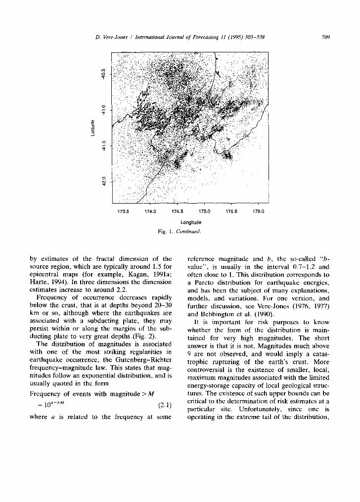
The distribution of epicentres over a geo- graphical region is usually very irregular. On the largest scale this is seen in the clustering of .earthquakes along plate boundaries and similar global features, but persists also on smaller scales (Fig. 1). In this visual sense the spatial patterns exhibit self-similarity. This is confirmed
• " ' " ' . ' I
tD e?,
. J
O v
170 172 174 176 178 180
Longitude
Fig. 1. (a) Earthquakes with M/> 3 in the main seismic region of New Zealand, 1987-1992. (b) Microearthquakes with M/> 2 in the Wellington region, 1978-1992.
D. Vere-Jones / International Journal of Forecasting 11 (1995) 503-538 509
tq. 0
o. z,
z
Q
_1
173.5 174.0 174.5 175.0
Longitude
Fig. 1. Continued.
175.5 176.0
by estimates of the fractal dimension of the source region, which are typically around 1.5 for epicentral maps (for example, Kagan, 1991a; Harte, 1994). In three dimensions the dimension estimates increase to around 2.2.
Frequency of occurrence decreases rapidly below the crust, that is at depths beyond 20-30 km or so, although where the earthquakes are associated with a subducting plate, they may persist within or along the margins of the sub- ducting plate to very great depths (Fig. 2).
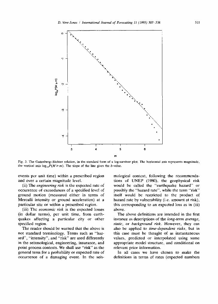
The distribution of magnitudes is associated with one of the most striking regularities in earthquake occurrence, the Gutenberg-Richter frequency-magnitude law. This states that mag- nitudes follow an exponential distribution, and is usually quoted in the form
Frequency of events with magnitude > M
= 10 a-bM (2.1)
where a is related to the frequency at some
reference magnitude and b, the so-called "b- value", is usually in the interval 0.7-1.2 and often close to 1. This distribution corresponds to a Pareto distribution for earthquake energies, and has been the subject of many explanations, models, and variations. For one version, and further discussion, see Vere-Jones (1976, 1977) and Bebbington et al. (1990).
It is important for risk purposes to know whether the form of the distribution is main- tained for very high magnitudes. The short answer is that it is not. Magnitudes much above 9 are not observed, and would imply a catas- trophic rupturing of the earth's crust. More controversial is the existence of smaller, local, maximum magnitudes associated with the limited energy-storage capacity of local geological struc- tures. The existence of such upper bounds can be critical to the determination of risk estimates at a particular site. Unfortunately, since one is operating in the extreme tail of the distribution,

510 D. Vere-Jones / International Journal of Forecasting 11 (1995) 503-538
o -
8 "7,
J ~
Q "7,
• . . • . : , . . . . ; : : ~ ' ~ : ~ = f . - ; . , . , , ~ . a . , ~ . . . . . " . ~ ~ . . . : ,.' .-. :~ :..':i-'_ . . . . .... ~ ...... - , , ~ ~ ~ ~ ' .
• , . : : , I " ! . ~ ! ! ~ ~ 8 ~ L :
• ,. ,',',,':;~ ..... : ..: ".~.?;~!~'~,~."
"..::/.'.i:~.~ ' ~ , " . ~ "'" " ." ." "
• ,~.=...~,~. ~.¢~.'... ~ .... . . . . ' . : . , , ~ . . ' , . ~ -
• .." " " :~: ' ; r :~ ' " ." "
. . . " : i . . . 7 " ' ~ ' ~ . ' " ' : ' • . . . . . , ~ . . . , , . . . . . .
• ..: :;.,i:'..':,;, ~.
• . . " . - ' -
I I I
170.5 171.0 171.5 172.0 172.5 173.0
latitude * sin(-30) + longitude * cos(-30)
Fig. 2. The depth distr ibut ion o f microearthquakes in the Wel l ington region. Same data as in Fig. l ( b ) fo r a cross-section look ing 23.5 ° E o f N (corresponding to the t ransformat ion t = lat i tude x sin ( - 30 °) = longi tude x cos ( - 30°)).
the data is usually insufficient to distinguish clearly between models for the upper tail, or to estimate at all reliably the value of a possible upper-bound. One form with some theoretical backing (see Vere-Jones, 1977; Kagan, 1991b) corresponds to the energy distribution with tail probabilities of the form
P(energy > E) = c E - ~ e -~E (2.2)
One other pronounced statistical regularity concerns the decrease of frequency with time along an aftershock sequence. This again follows a power law form, and is usually well modelled by a non-homogeneous Poisson process with rate function (intensity) of the form
A(t) = (c + t ) -o+a) (2.3)
where c and 8 are constants specific to the sequence but usually small, so that the simplest fo rm A(t)[oct-1], first discovered by Omori
(1894), is often an adequate approximation. Again there are many explanations and varia- tions of the model. In a general sense the power law distributions associated with both the Guten- berg-Richter and Omori laws bear witness to self-similar properties of the ear thquake process.
2.3. Varieties o f r isk
The term "ear thquake risk" is used loosely in a variety of senses, and we shall at tempt to distinguish between these. The principal distinc- tion we shall make depends on whether (like a geophysicist) one is concerned with the occur- rence of earthquakes per se, or (like an en- gineer) with the effects of ground motion, or (like an economic planner or insurance special- ist) with the costs of damage. This leads us to make the following distinctions.
(i) The geophys i ca l r isk (or e a r t h q u a k e h a z a r d )
is the expected rate of occurrence (number of
D. Vere-Jones / International Journal of Forecasting 11 (1995) 503-538 511
E
0- o
% 0 %
e ~
I I I I
3 4 5 6
e'•
in
Fig. 3. The Gutenberg-Richter relation, in the standard form of a log-survivor plot. The horizontal axis represents magnitude, the vertical axis log~oP(M/> m). The slope of the line gives the b-value.
events per unit time) within a prescribed region and over a certain magnitude level.
(ii) The engineering risk is the expected rate of occurrence of exceedances of a specified level of ground motion (measured either in terms of Mercalli intensity or ground acceleration) at a particular site or within a prescribed region.
(iii) The economic risk is the expected losses (in dollar terms), per unit time, from earth- quakes affecting a particular city or other specified region.
The reader should be warned that the above is not standard terminology. Terms such as "haz- ard" , "intensity", and "risk" are used differently in the seismological, engineering, insurance, and point process contexts. We shall use "risk" as the general term for a probability or expected rate of occurrence of a damaging event. In the seis-
mological context, following the recommenda- tions of U N EP (1980), the geophysical risk would be called the "ear thquake hazard" or possibly the "hazard rate" , while the term "risk" itself would be restricted to the product of hazard rate by vulnerability (i.e. amount at risk), this corresponding to an expected loss as in (iii) above.
The above definitions are intended in the first instance as descriptions of the long-term average, static, or background risk. However , they can also be applied to time-dependent risks, but in this case must be thought of as instantaneous values, predicted or interpolated using some appropriate model structure, and conditional on relevant prior information.
In all cases we have chosen to make the definitions in terms of rates (expected numbers

512 D. Vere-Jones / International Journal of Forecasting 11 (1995) 503-538
per unit time) rather than probabilities. One of the difficulties in using probabilities directly is that they are tied to specific and essentially arbitrary intervals or windows. Standardising the time interval, in order to facilitate comparisons, is tantamount to working in rates, at least if the time interval is small.
Working in rates also avoids a premature commitment to a specified model. Most en- gineering and insurance applications use static background rates, and these can be estimated from simple average frequencies. The prob- abilities, on the other hand, have to be calcu- lated assuming either the Poisson model or some alternative to it, introducing what may be gratuitous assumptions concerning the model. Of course, some commitment to a model will ulti- mately be needed, in order to develop predic- tions, but even here, statements in terms of expected rates rather than probabilities facili- tates comparisons.
The ratio between a local short-term rate and the long-term background rate we shall call the risk enhancement factor (Kagan and Knopoff, 1977; Vere-Jones, 1978). It is analogous to the probability gain of Utsu (1979, 1983) and Aki (1981), which is a ratio of the probabilities for some agreed region and observation interval; the probability gain reduces to the risk enhancement factor when the intervals are small. Other terms used are the risk refinement factor (Rhoades and Evison, 1979) and hazard refinement factor (Evison, 1984). Depending on circumstances, the risk enhancement factor may be greater or less than one; in the latter case we may also talk about the risk reduction factor. For risk forecasts to have significant practical consequences, such factors need to reach an order of magnitude or SO.
There is an important logical progression be- tween the three types of risk defined above.
The geophysical risk is the province of the scientist and the main focus of the present paper. It relates directly to the physical processes caus- ing earthquakes.
Estimates of the engineering risk can be de- rived from estimates of the geophysical risk. Granted the occurrence of an earthquake of a
particular size at a particular source, "attenua- tion factors" can be used to estimate the am- plitude of ground motion at a particular site. The overall risk at the site can then be obtained by summing (integrating) the contributions from different possible sources. Additional complex- ities arise from the effects of soil conditions (micro-zoning), the focusing effects of local topography or geological structures, the fre- quency content of the seismic waves, directional effects, etc. A standard reference to this stage is Cornell (1968); see also Cornell (1980), Vere- Jones (1983), Veneziano and Van Dyck (1987).
The final stage uses the estimated levels of ground movement to forecast the extent of damage to particular types of structure and hence to estimate the economic losses in dollar terms. This stage is fraught with even greater uncertainties than the other two. The usual approach is to try and estimate "damage ratios" for a given type of structure subjected to a given level of shaking. These represent the cost of damage as a proportion of the value of the structure. Expected losses can then be estimated by multiplying values by damage ratios and summing over the different structures at risk. Dowrick (1991) and Dowrick and Rhoades (1993) present detailed analyses of damage ratios arising in a recent New Zealand earthquake.
Even when these primary losses have been estimated, there remains the problem of losses due to secondary effects, particularly fires. These are yet more difficult to assess, and more vari- able, than those associated with the direct effects of the ground motion. In practice, simulations generally offer the best way of combining models for the geophysical and engineering risk with the particularities of a given portfolio, and are al- ready widely used in the insurance and reinsur- ance industries (for example, Rauch and Smolka, 1992).
For the remainder of this article we shall concentrate on the problems of forecasting the geophysical risk. It is the centre of scientific effort in this field, and is where the modelling component originates. In reality, however, the three aspects cannot be fully separated, but together form part of a tangled web of scientific,

D. Vere-Jones / International Journal of Forecasting I1 (1995) 503-538 513
engineering, economic, political, administrative, and social issues.
3. The point process framework
To develop and compare the performances of particular models of earthquake risk, it is essen- tial to have available a sufficiently extensive and flexible theoretical framework. For the geophysi- cal risk in particular, the natural framework is that provided by the theory of random point processes. This is a point of view I have long advocated (see for exampte, Vere-Jones, 1970, 1978), but it has yet to be fully exploited in the field of earthquake prediction. One reason may be that not only are probabilistic methods in general relatively new to earthquake prediction, but point processes in particular require different forecasting procedures to those commonly used in other branches of time series. Traditional time series methods are based on the linear predic- tions which are optimal for Gaussian processes. Forecasting the time to the next event is essen- tially a non-linear problem, however, and the distributions involved are often far from Gaus- sian. None the less quite general and flexible methods of forecasting point processes are now available, closely related to the "Cox regression methods" (Cox, 1972) used in reliability and other contexts for modelling the effects of exter- nal factors on life distributions.
In this section we provide an introduction to the most important ideas needed to develop forecasting procedures in the point process con- text. There are many texts on point processes which can be referred to for further details - see, for example, Cox and Lewis (1966), Snyder (1975), and Cox and Isham (1980) for modelling aspects, and Bremaud (1981) or Daley and Vere- Jones (1988) for the background theory. Snyder and Bremaud as well as Karr (1986), Kutoyants (1984) and Daley and Vere-Jones, all give ac- counts of the conditional intensity concept, which is central to the development both of forecasts and of simulations.
The point process context is relevant so long as the origin times can be treated as time
instants, with which the other variables can be associated. One then has a choice of treating the process as a point process in time (one dimen- sion), in time and space (three or four dimen- sions), or quite generally as a marked point process in time, the mark for each event con- taining information about all the other parame- ters it is desired to include in the study.
To develop a point process model it is neces- sary in principle to specify consistent joint dis- tributions for the random variables N ( A ) count- ing the numbers of events in subsets A of the chosen phase space (time, time × space, time x mark). The process is stationary in time if these joint distributions remain invariant under simultaneous and equal shifts of the sets A along the time axis.
The first and second moments of the random variables N ( A ) , are given by the set functions
re(A) = E[N(A)] m2(A x B) = E[(N(A )N(B))],
and play a specially important role. In the special case of a stationary point process in time alone, there exists a mean rate m (assumed finite and non-zero) such that
re(A) = mlA I
or, in infinitesimal notation
E[dN(t)] = m.dt
where IAI is the length (Lebesgue measure) of the set A. The second order properties of such a process are most conveniently stated in terms of a covariance density c(r) defined loosely by
Cov(dN(t), dN(t + ~')) = [c(r) + m6 (r)] dt dr.
Here the delta-function term m6(r ) arises from the point character of the process, which implies that E[dN(t) 2] is of order dt, whereas E(dN(t) dN(s)] is of order dt ds for t ~ s.
It is possible in principle to develop a second order prediction theory based on these concepts, (see, for example, chapter 11 of Daley and Vere- Jones, 1988) analogous in many ways to the second order prediction theory for continuous processes. It is useful, however, only for prob- lems in which the time scale is large compared

5 1 4 D. Vere-Jones / International Journal of Forecasting 11 (1995) 503-538
with the mean interval between events. Dis- tributions of the number of events N ( A ) then become more closely Gaussian, and the linear predictions which derive from the second order theory become closer to optimal. This is em- phatically not the case for predicting the time to the next event. Here it is more natural to focus on the sequence of time intervals between events, which will also be stationary, and to attempt to forecast the length of the current interval.
An immediate difficulty is the need to take into account the time which has already elapsed since the occurrence of the last event. If the intervals are presumed independent (i.e. form a renewal process) then one can work from the conditional distribution of the remaining life- time, given the time already elapsed. This dis- tribution is most conveniently represented in terms of the hazard function h(t), defined for lifetimes (i.e. interval lengths) by
h(t)dt = Prob(life ends in (t, t + dt)llife > t).
(3.1)
If the life distribution has density f ( t ) , and distribution function F(t), then
h(t) = f (t)/[l - F(t)]. (3.2)
One then has
P(life time > t + ~'llife > t) = exp - h(u)du
from which the expected residual lifetime, or any other characteristic of the distribution of the time to the next event, can be computed.
For a process of independent intervals, the hazard function embraces all the information about the structure of the process needed for predictions. In the general case this hazard function has to be conditioned, not only by the time since the last event, but by any additional information concerning the past history that may affect the distribution of the remaining time. It then becomes nothing other than the conditional probability intensity, or conditional intensity function
;t(tl:~t)dt
= E[dN(t)lpast history ~t up to time t].
More generally, for a marked point process in time
A(t, M [ ~ ) d t d M
= E[N(dt x dM)lpast history ~ ] ,
where the past history may now include infor- mation about the marks {Mi} (each of which may be a vector), as well as the times of past events. In fact it is possible to define the past history even more generally, to include information about external variables, or processes evolving in time in parallel with the point process being studied. The crucial problem is to determine how the conditional intensity depends on such past variables. This requires both physical and mathe- matical insights, and might be considered a crystallisation of Aki's concern that the scientist endeavour to find objective means of calculating probabilities of occurrence conditional on given precursory information.
Recognition of the crucial role of the con- ditional intensity function was a major turning point in the study of point processes, and may well be so for earthquake prediction also. Among its key properties are the following, where for simplicity we return to the one-dimen- sional case and contract the notation to A(t).
(i) A knowledge of the conditional intensity function, as an explicit function of the past, completely defines the probability structure of the process.
(ii) The log likelihood of a realisation (t 1 ...tN) in the time interval [0,T] is given by
T
f logL(t 1, t2, . . . , tN) = ~ log A(t l ) - A(u) du . i
0
(3.3)
This representation is of great importance because (under suitable regularity conditions: see Ogata (1978)) it allows the full machinery of likelihood methods to be used with conditional intensity models, including not only the standard estimation and hypothesis testing methods, but

D. Vere-Jones / International Journal of Forecasting 11 (1995) 503-538 5 1 5
also likelihood-based model selection criteria such as AIC (Akaike, 1974; Sakamoto et al., 1983).
(iii) If T* denotes the time to the next event, one can write
( ; ) P(r* >~- )=exp - A*(u)du (3.4) 0
where A*(u) is obtained by extrapolating A(t[~) forward from t to t + u under the assumption that no further event occurs in (t,t + u).
(iv) The above result allows A(t) to be used as a basis for simulations, in particular for simula- tion forward given a past history ~ . One then uses (iii) to generate a value of T*, adds the occurrence of the event at t + T* to an updated history ~ + r * , and repeats the simulation. For further details and alternative methods see Ogata (1981) and Wang et al. (1991).
(v) The differences dN(t) - Aft) dt integrate to form a continuous time Martingale. The con- ditional intensity therefore provides a link to the Martingale properties which have been of key importance in other branches of stochastic pro- cess theory. See the references cited earlier, especially Bremaud (1981) or Karr (1986), for further details and a more rigorous treatment.
(vi) In the special case of a stationary Poisson process, A(t) reduces to a constant A(=rn) independent of the past. This is the "lack of memory" property of the Poisson process: it has a constant risk, irrespective of the past occur- rence or non-occurrence of events.
It is very important for the applications to earthquakes that these results extend in a natural way to marked point processes (the background theory is in Jacod, 1975). In particular, the likelihood for a set of observed occurrences ( t l ,M0, (t2,M2), ..., (tN,MN) over the time interval (0,T) and a region of marks m becomes
log L[(t~, M~), (t 2, M2)...(tN, MN) ] = 7"
M F f
1 , J d 0 m
(3.5)
The forecasting and simulation properties also generalise in an obvious way, at least if the total intensity, fm A(t, m)dm = A(t) remains finite. To simulate the process, for example, one may generate first the time T* to the next event of any kind, using A(t) in place of A(t) in (iii) and (iv) above. A value of M, say M*, can then be generated from the density f*(m)=A(t+ T*,rn)/A(t+ T*). Adding the generated pair (t + T*, M*) to the history, one can then repeat the exercise, and so continue. Practical difficul- ties can arise near the boundaries, where in- formation may be missing, or in the extension to models with infinite total rates, but even in such cases the simulation can generally proceed with some approximations.
Such simulations provide a comprehensive view of the future of the process, from which it is possible to estimate the distributions for any quantities of interest, such as the time to the next event with a mark in some specified subset, the expected numbers of events within specified time and mark boundaries, etc.
A final extension, also of considerable impor- tance, is to situations where the conditional intensity depends on external variables as well as the past history of the process itself. In the earthquake context such external variables could include the coordinates of any precursor events, or the values of physical processes evolving concurrently in time. Within a comprehensive model, such variables would be modelled jointly with the point process. When a comprehensive model is not available, it may still be possible to develop explicit expressions conditional on the values of the external variables, much as is done in the Cox regression models referred to earlier (see Cox, 1972, 1975).
The formal simplicity of these extensions should not be allowed to disguise the fact that developing and fitting models in higher dimen- sions is never a simple task.
4. Estimating the background risk
As we indicated in Section 2, most engineering and insurance applications are based on esti-
516 D. Vere-Jones / International Journal of Forecasting 11 (1995) 503-538
mates of the long-term or background risk, assuming implicitly that the underlying processes are stationary. In this section we examine in somewhat greater detail the questions posed by estimating such rates. Even if one's concern is more with the time-varying rates, the back- ground rates are important as a reference against which short-term fluctuations can be gauged.
4.1. Sources of data
A fundamental question which arises in this context concerns the most appropriate source of information. There are at least four as listed below.
(i) Information from current instrumental catalogues.
(ii) Records of historical earthquakes. (iii) "Paleoseismological" evidence of large fault
movements preserved in peat bogs, stream offsets, uplifted terraces, etc.
(iv) Measurements of the relative motions of plate boundaries, from both geological and geodetic sources.
Each of these sources has its own weaknesses as a basis for estimating the occurrence rates of major damaging earthquakes. The catalogue records are generally too short to allow for direct estimates of the rates of large events, while extrapolation from the rates for smaller events begs the question of whether the relative rates remain constant. The records of historical earth- quakes are rarely complete, being subject to the vicissitudes of war, changing regimes, shifting trade routes and population centres, and to considerable uncertainties concerning mag- nitudes. The data from "fossil" earthquakes are restricted to major events causing large, perma- nent ground movements. This leaves unanswered any questions concerning smaller events, which may be highly damaging on a human scale but not yet large enough to produce fault breaks. It is also difficult to establish whether the move- ment really occurred in a single large event. Finally, use of the rates of plate motion raises unresolved issues concerning the proportion of that motion that is taken up by earthquakes, and
how the motion is divided when it is spread over a network of faults and a long period of time.
The fundamental dispute, which has persisted now for over half a century, and casts its shadow also over methods for earthquake prediction, is between the geological and seismological evi- dence; whether the major risk is associated with events on major, identified faults, or is more widely distributed as the seismological records of smaller events tends to suggest. The methodolo- gies appropriate to these two situations are widely different, and we consider each context briefly below, starting with the seismological approach. A final subsection looks at the role played by the Poisson model.
4.2. Estimating background rates from the catalogue data
This topic is of importance in its own right. It encompasses not only questions about time rates, but also about estimating the parameters in the frequency magnitude law, estimating and displaying the spatial distribution of seismicity, and investigating possible spatial variations in the distribution of magnitudes. In most of this work it is tacitly assumed that we are dealing with a model of "distributed seismicity"-that magnitude and space distributions have smoothly varying density functions which can be estimated by suitable averaging procedures.
To focus ideas, consider first a general station- ary, marked, point process in time, with finite overall rate m say. In our context, m would be interpreted as the overall rate of events lying within a defined observation region and over some threshold magnitude M 0. For any measur- able subset C of the mark space (i.e. earth- quakes falling within a given space and mag- nitude window) one can define also the average rate r e ( C) ~ m of events with marks falling into C. It is clear that re(C) is additive over disjoint subsets of the mark space, so that the normalised set function
II(C) = m( C) / m
defines a probability distribution over the set of marks. It may be called the stationary mark

D. Vere-Jones / International Journal of Forecasting 11 (1995) 503-538 517
distribution. In our context it will be a joint distribution of magnitude and epicentre. The aim is to estimate, not merely the overall rate m, but the set function m ( C ) or I I ( C ) .
For example, if the epicentral coordinates are ignored (data is pooled for the whole region), the resulting Gutenberg-Richter relation may be regarded as defining the (marginal) stationary distribution of magnitudes. As a probability distribution it is usually written in the form
P(Mag > MlMag/> Mo) = 10 b(g-Mo)
where M o is the threshold magnitude. Alter- natively, multiplying both sides by the overall rate gives
Frequency of events with Mag/> M
= lOa b(M MI)).
where lO a = m is the overall rate of events with Mag >/M 0. The parameters a (or m) and b can be estimated very straightforwardly from
= loglo ( N / T )
/) = (-M - M0) log10 e
where N is the total number of events with M > M0, T is the time interval covered by the catalogue, M is the average magnitude of events with M > M 0. Both estimates are method of moment estimates, and are also maximum likeli- hood estimates under the assumption that events are occurring randomly and independently in time. Some care has to be taken over details such as rounding of magnitude values (see for example, Vere-Jones, 1988).
As mentioned in Section 2 there is a consider- able literature devoted to variants on the simple Gutenberg-Richter relation and the closely re- lated question of whether or not there exist local upper bounds for the magnitudes. Space pre- cludes entering into details, but if the simple Gutenberg-Richter form appeared inadequate, one might use a truncated (censored) exponen- tial if the truncation point had been determined a priori on geophysical grounds, otherwise a 2-parameter form such as (2.2).
Somewhat analogous questions arise in es- timating the spatial distribution of epicentres,
which form the spatial component of the mark. Here, however, a parametric form is unlikely to be useful, and some form of non,parametric or semi-parametric estimate will generally be neces- sary. A range of non-parametric density estima- tion methods is now available (see, for example, texts such as Silverman, 1986; Stoyan et al., 1987; Ripley, 1988). The methods have been reviewed from the perspective of earthquake catalogues in Vere-Jones (1992). With one caveat (see below) they represent standard 2- or 3- dimensional procedures. A simple, and generally quite adequate, procedure, is that of kernel estimation. Here the spatial intensity (rate per unit time and area) at a point x is estimated by an expression of the form
X(x) - i kh(x - xi) - T i
where T is the time span of the catalogue, the x i are coordinates of the events in the catalogue (now lumping together the magnitudes) and k h is a 2-dimensional, usually isotropic, probability density with a variable scale parameter h (such as the standard deviation if k is taken to be isotropic normal). The corresponding probability density is obtained by dividing by the overall rate m = N / T . In either case the crucial decision is the choice of the bandwidth h, to give an optimal compromise between bias (caused by over- smoothing, h too large) and variability (caused by under-smoothing, h too small).
The caveat concerning the earthquake applica- tions relates to the assumption of independent observations which is incorporated into the stan- dard recommendations for the choice of h. In the present context, time and space clustering repre- sents a departure from this assumption which needs to be examined with some care. The aim should be to smooth over ephemeral clusters (which die away with time and are not repeated at the same location) but to preserve local regions of high intensity which persist over time. A rather crude approach to this problem, sug- gested in Vere-Jones (1992), is to choose h by a "learning and evaluation" technique, smoothing the first part of the catalogue with a given h, and scoring the pattern so obtained with the data in

518 D. Vere-Jones / International Journal of Forecasting 11 (1995) 503-538
the second part, finally choosing that h which gives the best score. See Kagan and Jackson (1994a) for a further application.
Alternatives to kernel estimation are the use of orthogonal expansions, and the use of splines. We refer to Vere-Jones (1992) for further details. An example of the application of more sophisti- cated techniques (Bayesian spline fitting proce- dures) is given by Ogata and Katsura (1988).
Whichever method is used, once estimates ,~(x) are available for a given location x, stan- dard routines can be used to evaluate )~ (x) on a grid of points over the observation region, and to produce 3-D or contour plots from these. In- deed, ad hoc methods of this kind have long been used by seismologists and earthquake en- gineers to produce contour plots, not so much of the geophysical risk, but of the engineering risk. These are most commonly displayed as contour plots of the intensity or ground acceleration likely to be exceeded with a given low probabili- ty, in a given period, or conversely as contour plots of the expected return time for a given level of shaking. See, for example, Algermissen et al. (1982) and Basham et al. (1985). A series of more recent examples, which illustrate differ- ent approaches and technical points, is contained in Berry (1989).
An important issue of principle is whether the spatial distributions for low magnitude events are similar to those of high magnitudes, or, equiva- lently, whether b-values vary with space. For these purposes the joint distribution of epicentral location and magnitude is needed. From a computational viewpoint, the easiest approach is probably to write the joint rate in the form
A(x, M) = A(x)f(MIx)
where f (Mlx ) is the conditional density for magnitudes, given a location x, and A(x) is the marginal epicentral intensity. Assuming f (MIx ) retains the exponential form, estimating f (Mlx ) reduces to the problem of estimating spatial fluctuations in the parameter b, which can be regarded as a problem of non-parametric regres- sion. This is the more obvious in that the estimate/~ is the reciprocal of mean magnitude,
so that tracking the variation of/~ as a function of x is equivalent to tracking the behaviour of the mean magnitude (-M - M0) as a function of x. Once again there is a family of procedures available, including versions of the kernel and spline procedures. The kernel estimate, for ex- ample, takes the form
~ ( x ) = E k h ( X -- Xi)
E ( M i - Mo)kh(x - xi)
representing the reciprocal of a weighted average of the magnitudes, with the weights decreasing as a function of distance from x. Again Vere- Jones (1992) gives further details, while Ogata and Katsura (1988) give an example using a Bayesian spline approach.
4.3. Rate estimates from the fault model
l'he main alternative to a spatially distributed model is to assume that events are restricted to a network of more or less well-identified faults.
There are two lines of evidence supporting this point of view. The first is the abundant evidence associating fault movement with the occurrence of large earthquakes. The second is the more recent evidence quoted in Section 2 that the fractal dimension of the source region of earth- quakes, even when calculated from catalogue data, is significantly below the nominal dimen- sion of earthquake epicentre maps. Such results might be expected if events were concentrated on a network of fault planes, but the interpreta- tion is not completely transparent and other explanations may also be possible.
Many procedures for estimating the engineer- ing risk are based on identifying major active faults and estimating the mean return times for major events on each. Recently this view has been narrowed by supposing that any given fault or fault segment is characterised by events of a particular magnitude (or slip). The main evi- dence for this "characteristic earthquake" hy- pothesis comes from the records of "fossil" earthquakes, as outlined in Section 4.1. It has several times been suggested that the events
D. Vere-Jones / International Journal of Forecasting 11 (1995) 503-538 519
recorded in this way appear to be roughly constant in both size and return time (see for example, Sieh, 1981; Schwarz and Coppersmith, 1984). The direct seismological evidence for such a viewpoint is scanty, but reports have been given of similar sequences of events in particular locations (Bakun and McEvilly, 1984).
An apparent objection to such a model is that it contradicts the immense amount of data sup- porting the usual frequency-magnitude law. One possible response is that the frequency-mag- nitude law may not reflect the size distribution of earthquakes on a given fault, but the size dis- tribution of faults. This interpretation has the advantage of linking the self-similarity observed at the geographical level to the power law form of the frequency-magnitude law. It is an idea that has been part of the folklore for some time (see for example, Lomnitz' contribution to Vere- Jones (1970) and the author's reply). Since the surface break of a fault may not indicate its real size, while most of the smaller faults would not even reach the surface, the two hypotheses of distributed and fault-linked seismicity may be harder to separate than one might at first im- agine.
If the characteristic earthquake hypothesis is accepted, then estimating the background rate of events on a given major fault is reduced to counting the number of events on the fault, and dividing by the time interval. Where the number of events is insufficient, evidence from the plate motion, coupled with some estimate of the likely size of the characteristic earthquake on the fault, provides a second more indirect route. Neither method is very reliable. The major review by Kagan and Jackson (1994b) suggests that current estimates based on these procedures may be exaggerated, and calls into question the whole basis of the characteristic earthquake hypothesis.
4.4. A note on the Poisson m o d e l
The reader may be surprised to find this topic left until the end of the section, given that the Poisson model is widely treated as the default option by seismologists, engineers, and insurance
workers, and that it figures extensively in nearly all discussions of the engineering and economic risks.
The reason is related to a comment made earlier, that a large part of the discussion can be carried out directly in terms of mean rates, or mean return times, implying that under the assumption of stationary, the exact choice of model is immaterial. The Poisson assumption enters only when it is desired to compute prob- abilities from the mean rate m, which is then done according to the exponential formula
Prob(no events in (t, t + x)) = e-mX
In fact the probabilities as such rarely play an important operational role. They have become accepted in decisions concerning design at least partly as a matter of convention. Provided the Poisson formula is always used to compute the probability, there is (for a given design period x) a 1:1 monotonic relationship between rates and probabilities so that in effect the decisions are based on an assessment of rates.
The fact that the Poisson model plays the default role is to be expected. It is the "maxi- mum entropy" model (i.e. making least assump- tions in some sense) for a point process with given rates, and arises as the result of many "information-reducing" transformations of a point process (see Daley and Vere-Jones (1988) chapters 9 and 11 for more discussion of these ideas).
In particular, the engineering risk is usually the result of summing the contributions to the risk from a number of near-independent sources. It is well known that the superposition of se- quences of events from several independent sources approximates a Poisson process (see for example, Daley and Vere-Jones, 1988). Hence, the combined point process of exceedances of a given level of ground motion at a given site is likely to be closer to Poisson than the component from any individual source region.
Although the effects of departures from the Poisson model would tend to become more pronounced at very small probability levels, the author has argued elsewhere (Vere-Jones, 1983; see also McGuire and Shedlock, 1981) that even

520 D. Vere-Jones / International Journal of Forecasting 11 (1995) 503-538
here other errors and uncertainties are likely to swamp those deriving from departures from the Poisson model.
The net result is that while the Poisson model plays an indispensable role in guiding the discus- sions of risk into sensible channels, it is not usually a critical assumption for operational decisions based on the background risk: if any- thing it tends to provide a somewhat conserva- tive source of estimates.
This situation, however, alters drastically when we approach the realm of time-dependent risks. The constant risk or lack-of-memory prop- erty of the Poisson model is contradicted, albeit in different directions, both by the prevalence of clustering, and by the characteristic earthquake model. Any proposal for earthquake prediction will be measured in the first instance by the extent of its improvement over the constant-risk Poisson model.
5. Time-varying risks- general issues
5.1. A n overview
As soon as we enter the domain of time varying risks, new and difficult issues arise. Some of these are as follows.
(i) Because of the relative paucity of data relating to large damaging earthquakes, direct estimation of the relevant conditional intensities, or conditional probabilities, for such events becomes very difficult. To a much greater extent than for the background risk, estimates of any form of time-varying risk are likely to be strongly model-dependent. The model-based approach takes advantage of model structure to reduce the number of parameters that have to be estimated, thus allowing the existing data to be used more effectively. The corresponding disadvantage is that model-validation becomes a major concern in its own right. Different models, leading to different prediction scenarios, may be supported to a similar extent by the data. At the present time, there is no general agreement as to the most appropriate model to be used for time-
varying forecasts of the risk from large earth- quakes.
(ii) As we would see it, in an ideal situation, the proper sequence of events would be: first, model development and model validation; sec- ond, development of time-varying risk forecasts based on the selected model; third, development of earthquake alerts based on the risk forecasts. The actual situation presents a considerable distortion of this sequence. The main emphasis has immediately jumped to the stage of develop- ing and testing prediction algorithms, often with- out the development of proper physical or statistical models, and without realistic discus- sion of the operational use of the predictions. Two main reasons may be suggested for this premature (as it seems to me) emphasis on predictions: the great difficulty of developing physical models; and the social and political pressures on scientists to develop successful prediction procedures.
(iii) The discussion of earthquake prediction is further muddied by ambiguities in just what a prediction means. In some discussions it may mean nothing more than a calculation of prob- abilities, a forecast of the time-varying risk. By contrast, a formally announced prediction inevitably takes on some of the character of an earthquake alert. Calling an alert, however, is essentially an economic and political decision. The emphasis on developing formal predictions has therefore placed the scientist in the awkward position of trying to carry some of the obliga- tions and responsibilities that more properly belong to local and national authorities.
(iv) The emphasis on validating prediction algorithms, as against the more general pro- cedure of model validation, produces the further danger that the former process may become equated to the latter. However, the optimal procedure for testing a particular algorithm may not be optimal for testing the model on which it is based. Moreover, by highlighting the problem of validating particular prediction algorithms, the possibility may be overlooked that existing models, despite their imperfections, can provide sufficiently reliable guidelines to initiate worth- while risk-reduction activities.

D. Vere-Jones / International Journal of Forecasting 11 (1995) 503-538 521
(v) Some approaches to prediction, in par- ticular the pattern-recognition approach, eschew the idea of models as part of a basic philosophi- cal stance. The aim is to be purely empirical, using only the data and mechanical search pro- cedures to identify and calibrate the thresholds for a prediction algorithm. In so far as they are assessed in terms of frequencies of success or failure (false alarms and failures to predict), such methods are still inherently probabilistic in character. Rather than accepting the prediction algorithm so obtained as a final result, it would seem more sensible to view the variables in- corporated in the algorithm as promising ingredi- ents for a more explicit model, and examine them carefully for their possible physical mean- ing.
(vi) As in the estimation of background risk, there is a need to distinguish between the geo- physical and the engineering risk. Earthquake alerts would seem more appropriately based on the latter; the scientist's task, on the other hand, is to produce models for a time-varying geo- physical risk. Earthquake predictions run the danger of confusing the two aspects.
(vii) Both the information needed in the pre- diction, and the kinds of actions to which the prediction may lead, depend strongly on the time horizon of the prediction. It is common in the seismological literature to distinguish at least three main time-scales: short-term and imminent predictions (anything from a few seconds to about a day); intermediate-term prediction (a few days to a few years); long-term predictions (a few years or longer). The implicit focus in this paper is on intermediate- and long-term predic- tions, although some methodological points may apply more generally.
It will be evident even from this incomplete list that moving to time-varying risks not only sharply increases the model-building difficulties, but has administrative and political overtones which cannot be ignored. In the remaining parts of this section, we shall look at three particular aspects in somewhat greater detail: the problem of calling an earthquake alert; the problem of validating models and prediction algorithms; and the problem of dealing with model uncertainty.
5.2. Calling an earthquake alert as a problem in optimal decision making
Several authors have recently considered earthquake prediction from this point of view, and pointed out that here also the conditional intensity, as defined in Section 3, plays a key role. The ideas were first raised in Ellis (1985), but have recently been considerably generalised, sharpened and extended in a series of papers by Molchan and others (Molchan, 1990, 1991, 1994; Molchan and Kagan, 1992). We present a brief outline of the basic argument.
The class of situations considered is restricted in the first instance to those where only three quantities are needed to describe the cost struc- ture, namely a - t h e cost per unit time of maintaining the
alert C~ - the cost of a predicted event (i.e. one falling
within the alert period) C 2- the cost of an unpredicted event (falling
outside the alert period) Then over some time interval of length T the
total costs have the form
S = al(A) + CIN(A ) + CzN(A ~)
: al(A) + C2N(A ) - (C 2 - CI)N(A)
where A is the interval over which the alert is called, l(A) is its length, N(A) and N(A c) are the numbers of predicted and unpredicted events respectively, and we assume C 2 > C 1.
The aim is to reduce the expected cost to a minimum.
We consider first the special case that the intensity function A(t) is continuous, and non- random, as in the case of a non-homogeneous Poisson process (see Fig. 4).
Suppose first that the period of the alert is to be restricted to a set A with given length l(A). Given A(t) and l(A), how best should A be chosen?
We claim that the optimal choice of A is obtained by gradually increasing the crossing level k (see the figure), thus decreasing the length of the interval on which A(t)/> k, until this length is just equal to the prescribed value l(A).
522 D. Vere-Jones / International Journal o f Forecasting 11 (1995) 503-538
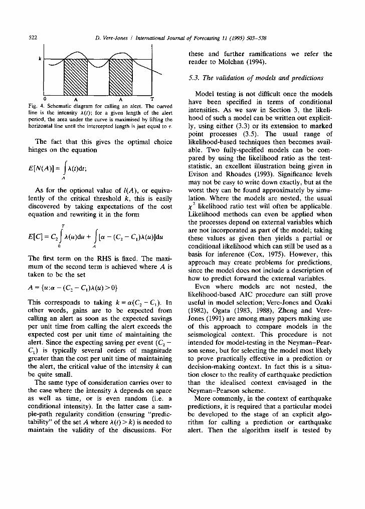
A A T Fig. 4. Schematic diagram for calling an alert. The curved line is the intensity A(t); for a given length of the alert period, the area under the curve is maximised by lifting the horizontal line until the intercepted length is just equal to ~'.
The fact that this gives the optimal choice hinges on the equation
E[N(A)I = fA(t)dt; A
As for the optional value of I(A), or equiva- lently of the critical threshold k, this is easily discovered by taking expectations of the cost equation and rewriting it in the form
T
etcl=c f + -(c2-c,)a(.)]du 0 A
The first term on the RHS is fixed. The maxi- mum of the second term is achieved where A is taken to be the set
A = {u:a - (C 2 - Cl),~.(u) > 0 }
This corresponds to taking k = a ( C 2 - C1). In other words, gains are to be expected from calling an alert as soon as the expected savings per unit time from calling the alert exceeds the expected cost per unit time of maintaining the alert. Since the expecting saving per event (C2 - C1) is typically several orders of magnitude greater than the cost per unit time of maintaining the alert, the critical value of the intensity k can be quite small.
The same type of consideration carries over to the case where the intensity A depends on space as well as time, or is even random (i.e. a conditional intensity). In the latter case a sam- ple-path regularity condition (ensuring "predic- tability" of the set A where A(t) > k) is needed to maintain the validity of the discussions. For
these and further ramifications we refer the reader to Molchan (1994).
5.3. The validation of models and predictions
Model testing is not difficult once the models have been specified in terms of conditional intensities. As we saw in Section 3, the likeli- hood of such a model can be written out explicit- ly, using either (3.3) or its extension to marked point processes (3.5). The usual range of likelihood-based techniques then becomes avail- able. Two fully-specified models can be com- pared by using the likelihood ratio as the test- statistic, an excellent illustration being given in Evison and Rhoades (1993). Significance levels may not be easy to write down exactly, but at the worst they can be found approximately by simu- lation. Where the models are nested, the usual X a likelihood ratio test will often be applicable. Likelihood methods can even be applied when the processes depend on external variables which are not incorporated as part of the model; taking these values as given then yields a partial or conditional likelihood which can still be used as a basis for inference (Cox, 1975). However, this approach may create problems for predictions, since the model does not include a description of how to predict forward the external variables.
Even where models are not nested, the likelihood-based AIC procedure can still prove useful in model selection; Vere-Jones and Ozaki (1982), Ogata (1983, 1988), Zheng and Vere- Jones (1991) are among many papers making use of this approach to compare models in the seismological context. This procedure is not intended for model-testing in the Neyman-Pear- son sense, but for selecting the model most likely to prove practically effective in a prediction or decision-making context. In fact this is a situa- tion closer to the reality of earthquake prediction than the idealised context envisaged in the Neyman-Pearson scheme.
More commonly, in the context of earthquake predictions, it is required that a particular model be developed to the stage of an explicit algo- rithm for calling a prediction or earthquake alert. Then the algorithm itself is tested by

D. Vere-Jones / International Journal of Forecasting 11 (1995) 503-538 523
recording, for a data set not used in developing the model, the numbers of successful predic- tions, failures to predict, and false alarms, and comparing these with the numbers that might be expected on the basis of a simple null hypothesis, usually that of a stationary Poisson process.
As mentioned earlier, exclusive reliance on testing prediction algorithms has several weak- nesses as a general prescription. It leads too easily to the validity of the model being judged by the success or otherwise of the particular prediction algorithm. The prediction, however, is based on specific thresholds-ideally, as dis- cussed in the previous section, on thresholds stated in terms of the conditional intensity. It may be quite possible for a model to be valid, but for the prediction to fail through a wrong choice of threshold, or to be suspended because for a given threshold, there is insufficient data to give significant resu l t s -a probable outcome when the predictions are tested on large events.
This approach also introduces, to some extent gratuitously, the technical problem of developing statistical procedures for testing prediction algo- rithms. A common problem is that successive events may not be independent, so that the simplest analysis, assuming successes and failures form independent Bernoulli trials, may be mis- leading. Rhoades and Evison have explored this issue in some depth (see, for example Rhoades, 1989; Rhoades and Evison, 1979, 1993).
In their analyses they generally suppose that specific precursors are available in the form of signals or alerts which occur as associated point processes. A more general approach may be needed if the physical variables incorporating the predictive information are themselves continu- ous. In such a case it is not obvious that first converting these signals into discrete forms, by setting thresholds, will generate optimal proce- dures, nor is it obvious, if such conversions are used, how optimal thresholds should be chosen. Moreover it would seem difficult to discuss such questions without the existence of a joint model for both the earthquakes and the associated processes, in which case the joint model itself should be tested, before any algorithms based on its use are developed.
As against this, it can be claimed that in any application of such importance, the performance of the final prediction algorithm needs to be checked directly, and independently of any ear- lier validations of the model. Kagan and Jackson (1991, 1994b) have rightly pointed to the difficul- ty of ensuring that the initial choice of data, especially threshold levels and geographical boundaries, does not have the effect of favouring (not necessarily wittingly), the data that best supports the model, thereby introducing a bias in favour of the model. Rhoades and Evison (1989) point to the need for a careful distinction be- tween subjective and objective stages of develop- ing a scientific model, and demand that the model verification stage be free of subjective elements. Even with the best intentions, how- ever, it is hard to avoid all forms of bias, so that continuing evaluation of the model and associ- ated algorithms, on new data, in actual use or in conditions as close as possible to actual use, is ultimately essential.
5.4. Dealing with model uncertainty
Even in the most optimistic scenario it seems unrealistic to assume that the model could ever be known exactly. Even if its general structure were known, parameter values would need to be estimated. The number of parameters required to define the model to an adequate degree of precision might also be uncertain. Finally, there might be uncertainty about the model structure. Competing model structures might be supported to a similar degree by the available data, but might lead to different forecasts of the time- varying hazard. What can be said about predic- tion in the face of such uncertainties?
First of all, it should be emphasised that in this respect earthquake prediction is not different in kind from other forms of statistical prediction. Even in the simplest example of prediction based on a regression, it is recognised that the predic- tion will be subject to error from two sources: the uncertainty inherent in the randomess of the predicted event itself (deriving ultimately from factors which have not been captured in the model) and that deriving from uncertainty in the
524 D. Vere-Jones / International Journal of Forecasting 11 (1995) 503-538
parameters. When predicting a characteristic of the distribution of the predicted event, such as its expected value, or the probability of the event exceeding a certain threshold, the former com- ponent drops away, but the latter remains.
Exactly this situation applies to predicting expected values or probabilities associated with earthquakes. The expected values and prob- abilities inherit the uncertainties implicit in the model formulation. Confidence intervals can be developed for such characteristics, just as for the model parameters. A Bayesian approach is likely to be the most flexible, in which the confidence interval would be derived from the posterior distribution of the characteristic in question. Nor is the Bayesian approach limited to situations where the only uncertainties relate to the param- eter values within a well-defined model. They can be extended to situations where the model itself is uncertain, by giving prior probabilities to each possible model, developing each model's posterior probability, and using these values to weight the posterior distributions arising from each model separately. The resulting mixture distribution can be used to define both a point estimate for the characteristic of interest, and an associated confidence interval. Indeed, almost exactly this procedure has been used by the Working Group on Californian Earthquake Probabilities (1988, 1990), although the models they included were restricted to versions of the time predictable model (see Section 6.2 below).
This raises an important issue. It is implicit in the guidelines for issuing predictions set out by NEPEC and other groups that the resolution of the problem of model uncertainty is seen in terms of model selection. Out of the many uncertain candidates presently offering them- selves, one or two will ultimately show superior performance, and will be selected as the basis of real-life prediction schemes.
In fact, this may not be the best approach in practice. The alternative is to think not in terms of model selection, but of model combination, probably using a Bayesian approach as suggested above. Rather as in the definition of economic- type indices, a "basket" of models could be selected, and weighted conditional intensity esti-
mates (or probabilities) prepared on the basis of these. Each model's likelihood would contribute to its posterior weighting, and from time to time the contents of the basket could be reviewed, dropping out old models that had not performed well, and replacing them with new ones which might do better. At any time, the resulting probability intensity would be available for use as an input to decision-making and disaster mitigation procedures. For further discussion of the problem of combining predictions see, for example, Clemen (1989).
6. Time varying risks: Some specific algorithms
Despite the massive literature on earthquake prediction, there are very few candidate pro- cedures which are based on models from which conditional intensities or probabilities can be calculated, and which at the same time have been tested on data, enjoy some semblance of credibility, and yield a significant sharpening of the risk over the Poisson model. Indeed, we know of none which satisfy these criteria fully. In this section we describe some of the best-known and more successful attempts.
6.1. The Hawkes process and Ogata's E T A S model
In the early 1970s, Hawkes (1971) introduced a family of what he called "self-exciting" or "mutually exciting" models, which became both pioneering examples of the conditional intensity methodology and models of general utility for the description of seismic catalogues. Early ap- plications to such data are in Hawkes and Adamopoulos (1973), and in the discussion of the "Klondyke model" in Lomnitz (1974). The models have been greatly improved and extend- ed by Japanese authors, especially Ogata, whose "ETAS" model was recently adapted for the IASPEI software programme (see Ogata, 1993). In his hands it has been successfully used to elucidate the detailed structure of aftershock sequences (Ogata and Shimazaki, 1984), the causal influence of events in one region on those

D. Vere-Jones / International Journal of Forecasting 11 (1995) 503-538 525
in another (Ogata et al., 1982; De Natale et al., 1988), the presence of trends and seasonal effects (Ogata and Katsura, 1986), and the detection of periods of relative quiescence masked by a background of decaying aftershock sequences (Ogata, 1992). A general introduction and re- view of the methodology is in Ogata (1988).
Basically the Hawkes process is a model for clustering, one of the most ubiquitous features of catalogue data. In the simplest context of a sequence of otherwise homogeneous events in time, the intensity takes the form
A ( t ) = a + ~ g( t - t . ) (6.1) n:ln<t
where a > 0 is a background immigration term; g(x) > 0 represents the contribution to the con- ditional intensity after a lag of length x, and satisfies J',~ g(u)du < 1, and the sum is taken over all events {tn} occurring before the current time t. The process has both epidemic and branching process interpretations. Any single event can be thought of as the "parent" of a family of later events, its "offspring", which ultimately die out but are replenished by an immigration compo- nent. Its motivation is essentially pragmatic, although Lomnitz (1974) points out the resem- blance to Boltzmann's original representation of "elastic after-effects" (Boltzmann, 1876) as a linear combination of time-decaying terms. In practice, g(x) is usually given a simple paramet- ric form, such as a finite sum of Laguerre polynomials (Vere-Jones and Ozaki, 1982), or the Pareto-type form used in Ogata's ETAS model, by analogy with Omori's law (see Section 2.1).
The model is readily extended to include additional variables. Magnitudes can be incorpo- rated in a marked point process intensity of the form
A(t,M)=f(M)[a + ,,:,,<t~ h(M,)g(t- t,)]
where f(M) is the marginal distribution of mag- nitudes (assumed constant and independent of past occurrences-Lomnitz's "magnitude stabili- ty" (Lomnitz, 1966))-and h(M) is a weighting
function which increases rapidly with magnitude (e.g. as exp(yM) for some 3' > 0).
The extension to "mutually exciting" pro- cesses takes the form
Ai(t)=ai + ~ [,,:~<gij(t-tn(J))]
where i = 1 . . . . . M, j = 1, ..., M are the different components, and gij for i ¢ j are transfer func- tions which determine the contribution to the risk of type i events from past events t,(j) in the jth component. Ogata et al. (1982) and de Natale et al. (1988) both use this approach to discuss the causal influence of events in one region on the occurrence of events in another. Again, mag- nitude terms can readily be added to the model.
The final extension is to replace the discrete index j by a continuously variable spatial coordi- nate x, which leads to a space-time-magnitude intensity of the form
A(t, M, x_)
-f(M)[a(x_)+ ,,:,<,Z h(M,)g(t-t,,x__-x,)],
where a(y_) is a spatially distributed immigration or background noise term, and g(t,x) is now a space-time kernel such as a Gaussian (diffusion) kernel. Further details and examples are given by Musmeci and Vere-Jones (1992) and Rathbun (1993). It is one of the very few examples of a full space-time model. Recently, however, Kagan and Jackson (1994a) have taken such ideas one step further by incorporating not only the location but also the orientation of the fault movement. In other respects their model is similar in spirit to, but different in detail from, the self-exciting models described here.
At present, models of this kind offer the best general purpose description for catalogues of moderate size (M t> 4 or M t>5) earthquakes. They are amply attested by applications to many different seismic regions. The time-magnitude version of the ETAS model, in particular, has been used very effectively in discussing seismic quiescence and related problems; see Ogata (1992), for example.
The disadvantage of these models from the point of view of earthquake prediction is that the

526 D. Vere-Jones / International Journal of Forecasting 11 (I995) 503-538
models have little predictive power. Insofar as g(x) is typically a decreasing function, the high- est risk is immediately following a past event. As the local activity increases in a region, so does the risk of further events. A typical history for the E T A S model is shown in Fig. 5 (after Ogata, 1988). Of course this feature is not to be read as a criticism of the model. It is either a fact of life, or a reason to look outside the catalogue, or for more particular patterns within it, for more effective precursory information.
6.2. Characteristic earthquakes and the time- predictable model
Recent discussions of ear thquake risk in Cali- fornia have been dominated by the "characteris- tic ea r thquake" model referred to in Section 4. This model has a very appealing simplicity. Every major fault, or fault-segment, is character-
ised by ear thquakes of a fixed size and fre- quency. The ideal characteristic ear thquake se- quence would have identical magnitudes, identi- cal fault mechanisms, and identical t ime intervals between successive events. In reality some vari- ability is introduced through uncertainties of measurement and perhaps of the physical pro- cess itself. This has led to the sequence of inter- event times being modelled either as a renewal process, or as a modified renewal process (" the t ime-predictable model" ) in which the t ime to the next event is taken to be proport ional to the size (in terms of observed displacement or slip) of the preceding event. The justification for this last assumption is that the time interval repre- sents the time taken to build up the stress along the fault segment to the critical value needed to rupture that segment again.
Let t*(t) and M*(t) denote the t ime and magnitude of the most recent event on the fault,
5
4
3
2
1
0
. . . . . . . . . . . . . . . . . . . . . . . . . . . . . . . . . . . . . . . . . . . . . . . . . . . . . . . . . . . . . . . . . . . . . . . . . i . . . . . . . . . . . . . . . . . . . i . . . . . . . . . . . . . . . . . . . ';. . . . . . . . . . . . . . . . . . . . :,. . . . . . . . . . . . . . . . . .
8 . . . . . . . . . . . . . . . . . . . . . . . . . . . . . . . . . . . . . . . . . . . . . . . . . . . . . . . . . . . . . . . . . . . . . . . . . . . . . . . . . . . . . . . . . . . . . . . . . . . . . . . . . . . . . . . . . . . . . . . . . . . . . . . . . . . . . . . . . . . . . . . . . . . . . . . . . . . . . . . 6 . . . . . . . . . . . . . . . . . . . . . . . . . . . . . . . . . . . . . . . . . . . . . . . . . . . . . . . . . . . . . . . . . . . . . . . . . . . . . . . . . . . . . . . . . . . . . . . . . . . . . . . . . . . . . . . . . . . . . . . . . . . . . . . . . . . . . . . . . . . . . . . . . . . . . . . . . . . . . .
0 1 O0 200 300 400 500 600 700 800
Time (days)
Fig. 5. A realisation of the conditional intensity from Ogata's ETAS model. The uppermost graph represents the cumulative curve J'0 A(t)dt, the middle graph is a plot of the conditional intensity A(t) itself, and the bottom plot shows the times and magnitudes of the largest events. The plot is produced from software developed by Y. Ogata and T. Utsu for the International Association for Seismology and Physics of the Earth's Interior (IASPEI).

D. Vere-Jones / International Journal of Forecasting 11 (1995) 503-538 527
or fault segment, prior to the current time t. Then if h(ulM) denotes the hazard function of the time between events, supposing the previous event had magnitude M, the conditional intensity function for events on that fault has the form
A(t) = h ( t - t*lM*). (6.2)
A detailed working through of this methodolo- gy to events affecting California in general, and the San Francisco Bay region in particular, are contained in the two USGS working group reports (Working Group on Californian Earth- quake Probabilities, 1988, 1990). The "engineer- ing risk" for a given site is then calculated by summing the risk contributions from each fault segment close enough to affect the site in ques- tion: thus the engineering risk (for a specified intensity of shaking) appears as a sum of terms
AE(t, x) = ~ a i ( x - --Xi, Mi)hi( t - t* IM*) i
where the a i are attenuation factors relating the site to the source i and characteristic magnitude M i of the ith source fault; ti* and Mi* are the time and magnitude of the previous event on that fault, and hi(u[M ) is the conditional hazard function for the ith fault.
In the specific formulation preferred by the Working Group, the role of the magnitude is played by the slip (displacement) on the fault and the inter-event distributions are taken to be lognormal, with median proportional to the slip of the previous event on the fault. The justifica- tion for the lognormal is indirect, deriving from analogies with in'er-event distributions from a variety of seismic sources.
The hazard function for the lognormal dis- tribution increases from zero to a maximum around the median and then decreases back to zero. Possible histories for the conditional in- tensity on a single fault, and for the engineering risk at a site affected by several faults, are shown in Fig. 6. Both seem to me somewhat counter- intuitive. Note that the latter is closer to constant than the former, as a consequence of adding the contributions from different sources (approxima- tion to a Poisson process).
As mentioned in Section 4, the most serious
difficulty posed by this model lies in the fact that it is not rooted in the catalogue of current earthquakes. The evidence in favour of the characteristic earthquake model is largely based on paleoseismological records. Even incorporat- ing historical events, there are rarely more than two or three direct records of events which have affected substantial segments of the major faults. Not only is the general evidence for the model indirect, but its parameters, such as the slip rate and the standard deviation in the lognormal distribution, also have to be inferred indirectly, usually from a consideration of geological and tectonic evidence.
This lack of connection with the seismic catalogue is illustrative of the seismologist's current dilemma. Is it reasonable to assume that the major events follow patterns and processes which cannot be directly confirmed from the catalogues? If so, what is the best method of combining such information with the catalogue data?
One reason for caution with models of this kind, illustrated all too vividly by the recent Northridge earthquake in Los Angeles, is that earthquakes quite large enough to pose a major hazard in human terms, may be insignificant in relation to the still greater events which take up the motion of the plates on a geological time scale. Indeed the third Working Group report, for Southern California, for which drafts are currently in preparation, adapts a mixed philosophy, looking at the risk both from large events along the major faults, and from smaller events in other locations.
6.3. Stress release models
The time-predictable model considered briefly in the previous subsection represents an attempt to capture, in terms of a stochastic model, the underlying idea of Reid's (1910) elastic rebound theory of major earthquakes. The "stress release model" developed in a series of papers by the author and colleagues (see Ogata and Vere- Jones, 1984; Vere-Jones and Deng, 1988; Zheng and Vere-Jones, 1991, 1994) attempts to provide a more general formulation of the same idea.

528 D. Vere-Jones / International Journal of Forecasting 11 (1995) 503-538
0
o
o4 ~ d
0 f / i i i i
0 5 10 15
time
0
o
o
o 0
/ i i i !
0 5 10 15
time
o
~ d
o
O ¢5
i ! i i
0 5 10 15
time
Fig. 6. (a) and (b) Schematic representations of the conditional intensity from the time-predictable model, (c) The result of superposing the risks from both sources.

D. Vere-Jones / International Journal of Forecasting 11 (1995) 503-538 529
This version was developed primarily for analys- ing regional historical catalogues, for events with M >/6 or 6.5, that could be considered reason- ably complete over a period of 3-4 centuries. Historical catalogues approaching this quality are available from Northern China, Japan, Italy, Iran, and possibly other countries. Here we shall outline a general formulation of the model and contrast the assumptions required to specialise it first to the time-predictable model of the previ- ous section, and then to the model used in the analyses of historical data mentioned above.
The first general assumption is that the prob- abilities of events occurring within the region (or on the fault) are determined by an unobserved state variable. In the versions of the model which have been developed so far it is supposed that this state variable can be represented by a scalar quantity X(t) which increases linearly between events and decreases instantaneously when events occur. It is not necessary that this quanti- ty be interpreted literally as stress but this is its general character. At any time, X(t) then repre- sents the balance between the accumulated tec- tonic stress in a region and the amount of stress released through earthquakes:
X(t) - X(O) = at - / 3 ~ S n . (6.3) n:tn<t
Two functions are then needed to complete the description of the model. One is a risk function t0(x) with the interpretation
to(x)dt -- Prob{event occurs in t, t + dtlX(t ) = x}
The second is a density kernel f (SIx) with the interpretation
f (S lx )dS
= Prob{stress release is in range S, S
+ dS[event occurs when X ( t ) = x }
All such models fall within the more general class of point processes for which the intensities are governed by an (unobserved) Markov pro- cess, in this case the process X(t) . Indeed, the conditional intensity here takes the form
A(t, S) = tp[X(t)]f(SlX(t)) . (6.4)
We are now in a position to examine the differences between the model variants. In the time predictable model ~0(x) has a singularity at the strength of the fault, say x0:to(x)=0 for x < x 0 and to(x)= 0o for x ~>x 0. By contrast, in the regional stress release model it is assumed that to(x)--e x, i.e. that there is a "soft" upper limit to the strength of the crust over the region or along the fault.
The more crucial difference, however, is in the form of the frequency-magnitude distribution. In the model for historical earthquakes, it is assumed that a version of the Gutenberg-Rich- ter law is valid. This is converted to a stress release distribution by taking f(slx)= C.S 8, with/3 of the order 1.5-2. The time-predictable model, however, was not intended to model catalogue data, but a sequence of events of roughly constant size (slip). Consequently, al- though magnitudes as such are not explicitly modelled in the Working Group reports, it is implicitly assumed that they are either equal to the magnitude of the characteristic earthquake, or normally distributed about it, leading to the lognormal distribution for the slips or the stress release.
A feature of the regional stress release model is that, although the smaller events make rela- tively little difference to the stress level and to the pattern of larger events, the generally high risks when the stress state is high gives rise to a form of clustering within the model, even though the episodes involving larger events are spaced out. Some risk patterns for the Northern China region, taken from Zheng and Vere-Jones (1991) are shown in Fig. 7. Because of the exponential form assumed for to(x) these have a cusp-like appearance, in contrast to the smoother peaks of the time-predictable model, which derive from the smoother shaped hazard function for the lognormal distribution.
6.4. The pattern recognition approach and the M8 algorithm
For the last two decades, the Russian earth- quake prediction group, headed by V. I. Keilis- Borok, V. Kossobokov, and others, has been
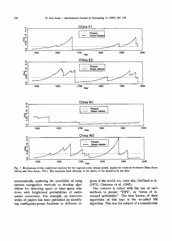
530 D. Vere-Jones / International Journal of Forecasting 11 (1995) 503-538
China E1
....... Poisson /
~!1~1 ~ - - S t r e s s R e l e a s ~
t 500 1600 1700 1800 1900 2000 Year
China E2
I Poisson I
1500 1600 1700 1800 1900 2000 Year
i t } China Wl o
o
n 'u3 o. o
o o
I ....... Poisson I Stress release
• " ~ - 1 . . . . . . . . . . . . . . . . . . . . . . . . . . . . . . . . . . . . . . . . . . . . . . . . . . . . . . . . . . . . . . . . . . . . . . . . '
1500 1600 1700 1800 1900 2000 Year
China W2 -Posson J 1500 1600 1700 1800 1900 2000
Year
Fig. 7. Realisations of the conditional intensity for the regional stress release model, applied to events in Northern China (from Zheng and Vere-Jones, 1991). The examples show diversity in the ability of the model to fit the data.
systematically exploring the possibility of using pattern recognition methods to develop algo- rithms for detecting space or time-space win- dows with heightened probabilities of earth- quake occurrence. For example, an extensive series of papers has been published on identify- ing earthquake-prone locations in different re-
gions of the world; see, inter alia, Gel'land et al. (1973), Cisternas et al. (1985).
Our concern is rather with the use of such methods to predict "TIPS", or "times of in- creased probability". The best known of their algorithms of this type is the so-called M8 algorithm. This was the subject of a considerable
D. Vere-Jones / International Journal of Forecasting 11 (1995) 503-538 531
furore in 1988, when the Soviet president indi- cated to his American counterpart that Soviet scientists had predicted a period of heightened risk for Southern California. The US National Earthquake Prediction Evaluation Committee was called into action to meet with the Soviet scientists and consider their predictions (see NEPEC, 1989). No immediate action was taken, but further evaluation of the algorithm continued and a number of reports have since appeared in which the algorithm is described and applied to different regions and with different data sets (see, for example, Brown et al., 1989).
In essence, pattern recognition procedures are a means of automatically sifting through large data sets to discover particular data combina- tions which occur repeatedly before events of interest, and are therefore to be considered as potential precursors of such events. The pro- cedures generally involve two stages, a learning stage, in which patterns of potential interest are identified, and a selection stage, in which those patterns are selected which "work" with an independent set of data.
The M8 algorithm makes use of four indicators which have been developed and selected over a considerable period. They comprise:
(i) the numbers of main shocks (retained after removing aftershocks by a standard win- dowing procedure) in a moving time inter- val of fixed length;
(ii) the rate of change of such numbers; (iii) a weighted sum of the mainshocks within
such a sliding window, where the weight associated with a given event is proportional to a fractional power of the energy release;
(iv) a numerical characteristic of aftershock ac- tivity within the moving window, namely, the maximal count of aftershocks from any aftershock sequence within the year preced- ing the end of the moving time window.
The first three of these indicators are repeated for events with a lower magnitude threshold, giving seven indicators in all.
All seven of these characteristics are then evaluated for a series of circles with fixed diam- eter (related to the magnitude threshold of the catalogue) and centred on a suitable grid. A TIP
is declared for one of these circles when, for three years in succession, at least one indicator from each of the four types (i)-(iv) exceeds its upper p% percentile (where p = 10% for types (i)-(iii) and p = 25% for case (iv)), and not more than one indicator fails to exceed the corre- sponding threshold. The TIP is declared for a 5-year period. For further details see, for exam- ple, Keilis-Borok and Kossobokov (1990a,b).
The authors of the algorithm emphasise its purely empirical character, and disavow the possibility of linking it to a model-based ap- proach, or even to explicit risk forecasts. How- ever, as Ellsworth suggested in the NEPEC (1989) discussion one can obtain a rough indica- tion of the risk enhancement factor associated with a TIP by comparing its predicted number of events (one) with the expected number within the same region and time interval from the background rate. According to Ellsworth this suggests a risk enhancement factor in the range 3-5, which is similar to that given by the models considered in the two preceding subsections. Moreover it might be argued that one of the main values of such an approach is in the clues it gives as to features which may indicate local changes in the risk environment, and which may be worthy of further study. Even as they stand, any or all of the indicators (i)-(iv) could be incorporated as regressands in a Cox-regression type model for the conditional intensity, and this type of modelling could be used to give a more direct evaluation of their predictive power.
6.5. The precursory swarm hypothesis
One particular pattern, of a similar general character to those above, has been investigated in considerable detail. This is the so-called "pre- cursory swarm", a group of intermediate size events, closely grouped in time, space, and magnitude, and followed after some interval by a larger event whose time, space, and magnitude coordinates can be roughly inferred from the characteristics of the preceding swarm. This idea has been investigated in a series of papers of increasing sophistication and complexity by Evison and Rhoades: in particular see Evison

532 D. Vere-Jones / International Journal of Forecasting 11 (1995) 503-538
(1977, 1982), Evison and Rhoades (1993). More- over they have used their experience with this idea to formulate and discuss more general aspects of hypothesis testing as it relates to earthquake prediction; see, inter alia, Rhoades and Evison (1979, 1993), Rhoades (1989).
The following points arise, and are typical of those associated with the testing of precursory phenomena. (a) An exact definition of the precursory event
is needed. In the present case this requires explicit statements of just what may or may not be considered a precursory swarm.
(b) Likewise an exact statement is needed of just what events are being predicted.
(c) The description of the model should include an expression for the probability distribution (e.g. in the form of the hazard function) of the time to the predicted event, after the occurrence of the precursor.
(d) From the information in (a), (b), and (c), a likelihood ratio can then be developed for testing the given hypothesis against the Pois- son as a null hypothesis. Note that the likelihood ratio subsumes the information concerning the numbers of successful predic- tions (precursors followed by appropriate events), false alarms (precursors not fol- lowed by an appropriate event), and failures to predict (events not preceded by precur- sors).
(e) Since the authors advocate a Bayesian ap- proach, updating formulae need to be de- veloped both for estimating the parameters within the model, and for evaluating the likelihood ratio referred to in (d). In general this will include procedures for updating the probabilities that the observed precursors are "valid" - i.e. will be followed by an appropriate event.
None of these points is entirely straightfor- ward. The definitions required for (a) and (b) are to some extent arbitrary, particularly insofar as they involve magnitude or distance thresholds. As pointed out earlier, it is difficult, in such a context, to separate out the problem of testing the model from the problem of testing the thresholds. Here, as in the definition of a "valid"
precursor, there may be no clear physical moti- vation for the thresholds chosen, so that one is back into the pattern recognition mode. In more complex settings, where several types of pre- cursor may be involved, one becomes entangled in the impenetrable logical thicket surrounding the independence relations among the precur- sors, and between them and the predicted event. The assumptions made here can drastically modify the risk enhancement factor, but may be virtually impossible to verify directly because of the lack of data on the joint occurrence of several of the precursors.
In the simple form of the precursory swarm model described in Rhoades and Evison (1979), the magnitude M of the predicted event, and the time T to its occurrence from the occurrence of the swarm, are given by logarithmic regressions of the form
log T = a o + a i M + E 1
M = b 0 + bl log T + b 2 l ogM + E 2
respectively, where M is the average magnitude of the three largest events in the swarm, E 1 and E 2 are normally distributed error terms. As in Section 6.2 the lead times are lognormally dis- tributed, which according to Rikitake (1976) is typical of a range of longer-term precursory phenomena.
This simple form of the hypothesis was tested over some twelve years, and ultimately rejected when its likelihood ratio, relative to the Poisson, fell below a 5% level. According to Evison and Rhoades (1993) the reasons for its failure hinge on the narrow definitions required in (a) and (b), in particular by the inability of the model to cope satisfactorily with clusters of swarms and clusters of mainshock events. A more sophisticated ver- sion of the model, described in Evison (1982), is still being tested.
Despite the difficulties in formulating and testing a precise hypothesis, there is evidence from many regions that something akin to a precursory swarm occurs before many major events in many seismic regions. Such features may indicate a change in the underlying stress regime, and it is possible that something like a

D. Vere-Jones / International Journal of Forecasting 11 (1995) 503-538 533
hidden Markov model (for the stress regime) could provide a more flexible modelling frame- work within which such precursory features could be explored.
6.6. The Chinese experience
The one widely accepted example of a success- ful prediction, which established earthquake prediction as something more than a seismolog- ist's pipe-dream, occurred in Haicheng, in Northern China on February 4, 1975. According to Bolt (1988), on the day before the earth- quake, 'the Shihpengyu Seismographic Station suggested that the (recent) small shocks were the foreshocks of a large earthquake. As a result, on February 4, the party committee and the re- volutionary committee of Liaoning province alerted the entire province. Special meetings were held at once to ensure that precautionary measures would be taken. The people were mobilised to build temporary living huts, move patients from hospitals, concentrate transporta- tion facilities and important objects, organise medical teams, induce people to evacuate their homes, and move the old and weak to safety'. Then, at 7.36 pm, an earthquake of magnitude 7.3 struck the Haicheng-Yingkow region. West- ern as well as Chinese reports confirmed that the damage had been extensive, but that as a conse- quence of the prediction the losses of human and animal lives had been greatly reduced.
Subsequent analysis of this dramatic episode suggests that cultural and political factors played as big a role in this success as the information available to the Chinese seismologists. At that time in China, earthquake surveillance was a high priority among the lay population as well as among the specialists, leading to a high level of local involvement. Some years previously a period of relatively high activity had been noted, followed by a quiescence. Then, not long before the earthquake itself, activity began to recover, and to migrate towards the future epicentre. Finally the larger shocks occurred which were identified as foreshocks. Supplementary reports of anomalous animal behaviour, changes in
groundwater level, and direction of ground tilt- ing, etc, supported the conclusions, and rein- forced the decision to call the alert. Indeed, Lomnitz (1994) suggested that the public may have been leading the seismologists, rather than vice versa. In any case it seems that the decision was taken following the "step-by-step" procedure - initial information confirmed at each step by further evidence-favoured by the Chi- nese, and descriptive of a mode of decision- making rather than a method for computing risks, geophysical or otherwise. Such an interpre- tation is supported by the fact that, although the Chinese have claimed other successful predic- tions (see Cao and Aki, 1983; Ma et al., 1990), none have had the same impact. There have also been some tragic failures, notably in respect of the even greater Tanshang earthquake, which occurred the following year with a reported death toll of 250,000.
An attempt to quantify retrospectively the risks which might have been calculated from the information available at the time of the Haich- eng earthquake was made by Cao and Aki (1983). They first identified four types of pre- cursory information: long term (periods of gener- ally high activity); intermediate term (enhance- ment of moderate earthquake activity); short term (variation of radon content of water from a well); imminent (reports of anomalous animal behaviour). Then they calculated a rough risk enhancement factor (probability gain) for each, and multiplied the results to obtain a total risk enhancement of about 14,000. The largest contri- butions came from the terms corresponding to animal behaviour and radon content.
It is difficult to give much credence to this value, which vastly exceeds any of the estimates considered in the previous subsections. The estimates for the individual risk enhancement factors are very rough and the evidence support- ing them is not supplied in detail. Also the multiplication of these factors implies indepen- dent precursors, and can lead to a gross inflation of the risk enhancement if in fact the effects are not independent (see Rhoades, 1989). The calcu- lations do, however, suggest the important moral that continued monitoring of a wide range of

534 D. Vere-Jones / International Journal of Forecasting 11 (1995) 503-538
potential precursors may be an essential pre- requisite to successful earthquake prediction.
7. Concluding remarks
To what extent does earthquake forecasting raise unique problems and to what extent does it share features in common with other forecasting contexts? I hope that, after reading thus far in the article, readers with expertise in other fields of forecasting might be better able to answer this question than I am. By way of concluding remarks, however, let me give a personal impre- ssion of the situation.
As with any forecasting task there are two aspects to consider: what forecasting information is really wanted, and what technical tools are needed to supply it from the available data. As a proper statistician should, I put the question of use first: until the real uses have been clarified, no statistical investigation is likely to be effec- tive, and any work undertaken may be wasted.
Who, then, actually wants forecasts of earth- quake risk, and why?
Here I have to admit that, if genuine users exist, they have been slow to identify them- selves. Indeed, looking at earthquake prediction from this point of view, we quickly encounter two of the main problems which bedevil the subject: the high stakes for which the game is played, and the long-term character of the in- vestments that have to be made. Earthquake countermeasures are not cheap to put into place and it may be many years before they show their value. There will always be vested interests wanting to opt out of expenses which may be in the long-term public interest, but show little in the way of direct benefits. Perhaps for this reason, I know of little stated interest in risk forecasts which provide time-dependent risk en- hancement factors in the range 1-10, although this might seem a realistic goal in the present state of knowledge, and, used appropriately, might lead to significant reductions in the losses caused by earthquakes.
At the same time the huge cost and high drama of a major earthquake encourages emo-
tional reactions to any precise prediction, sci- entific or otherwise, and increases the difficulty of utilizing predictive information in a rational and objective manner. Nor are the media slow to exploit the public interest in earthquake predic- tion, and if the episode ends up, as it often does, in making the scientists look foolish, then so much the better; they are becoming an increas- ingly popular target for public frustration of many kinds. Gori (1993) documents a recent example of the expenses, anxiety, and general confusion caused by a prediction that had no endorsement from any reputable seismological body. Administrators are hardly to be blamed for not knowing which way to jump in such situations. Their primary responsibility is to the constituencies they serve, and it is to their perception of the situation, rather than to the distant voice of the scientist, that they are likely to listen in moments of stress. Such incidents illustrate that earthquake prediction is caught up with social and political issues which in practice obscure and even override considerations of cost and the rational use of resources.
I doubt if earthquake forecasting is unique in facing problems of this kind, but it is surely an extreme case.
Similar reasons may lie behind the "s top-go" character of earthquake research funding, at least in the United States. Bruce Bolt remarks in a recent review (Bolt, 1991) that 'In terms of national welfare, it might be ex- pected that the risk involved in earthquakes would give special force to the claims for funds and resources for earth scientists, engineers, planners and others involved in enhancing seis- mic safety. Seismological history tells otherwise. Risk reduction is characterised by bursts of activity and political support following major earthquakes, and delay curves that have a half- life of a year or so before public interest re- cedes.'
My impression is that the most satisfying applications of statistical forecasting procedures in seismology are related to engineering situa- tions where a particular need has been more tightly identified. The task of forecasting the amplitude and other characteristics of the ground

D. Vere-Jones / International Journal of Forecasting 11 (1995) 503-538 535
motion at a particular site is the most familiar of these, and is incorporated in many important engineering and design procedures. A recent local example relates to the analysis of lifelines in the Wellington region and the location of particular points of vulnerability in case of a major earthquake affecting the region. Such studies usually involve no more than a careful evaluation of background rates, but there is surely scope for extending them by identifying also the facilities that could best make use of advance warnings of increased levels of local risk at different time scales. Looking at the forecast- ing problem from such practical perspective helps to identify the predictive information that will be most genuinely useful. As well as direct- ing scientific and statistical research into prod- uctive channels, such a programme can also help to strengthen the working links between sci- entists, statisticians, and administrators.
By contrast, looking for the ultimate earth- quake prediction algorithm may prove to be something akin to the search for the holy grail, rich in virtue and prestige, but somewhat lacking in useful outcomes.
Now let me turn to technical aspects of earth- quake forecasting. By far the greatest technical difficulty is simply the absence of any identified source of reliable predictive information. This is primarily the scientist's problem, but the statisti- cian may be able to help through improved methods of condensing and displaying the in- formation in multidimensional data sets, and in developing more effective procedures for evaluating models and prediction algorithms. The exaggerated swing from excessive optimism concerning the possibility of earthquake predic- tion to the current state of general pessimism is certainly due in part to a failure to appreciate the statistical nature of the subject; neither extreme is really an appropriate response.
Leaving the fundamental scientific problem aside, forecasting earthquakes differs from most routine forecasting problems in that it deals not with a discrete or continuous time series, but with sudden random events. But, although prob- lems of this kind may be relatively uncommon in forecasting practice, they are certainly not un-
known. In essence, they fall into the same category as forecasting lifetimes, for which there exist substantial literatures in the engineering (reliability), actuarial, and medical contexts. In any such situation, the central concept is likely to be the hazard function (conditional intensity function, age-specific mortality rate) conditioned by relevant supplementory informatian.
A more significant technical difficulty, in my opinion, is posed by the spatial dimension of earthquake occurrence. Then there is no clearly defined "next event", as this will depend on the region the user has in view (not to mention also the magnitude threshold and possible constraints on other earthquake characteristics). One is forced into forecasting a space-time intensity, which stretches both models and algorithms to the limit. Indeed, full space-time models, for earthquakes or anything else, are rare. Only in epidemiology, to my knowledge, do similar problems arise, with somewhat similar models and procedures currently being developed.
Even here, therefore, the technical difficulties in developing space-time earthquake forecasts are not unique, although near the edge of current statistical and computing capabilities.
To summarise, there is little doubt that earth- quake prediction remains one of the most chal- lenging problems in contemporary science. It is still conceivable that a breakthrough will occur- that some precursory phenomenon will be dis- covered which will allow alerts to be called with a high level of confidence and precision. It seems more likely, however, that the emerging picture will be one of gradually tightening precautionary measures-low-level alerts which can be locally shifted to a higher level in response to sharpened estimates of the earthquake risk.
Acknowledgements
I am grateful to the Editor for suggesting the preparation of this article, and for his encourage- ment and helpful criticisms along the way. I am also indebted to a number of colleagues who read and commented on an early version of the article, in particular to Frank Evison and David
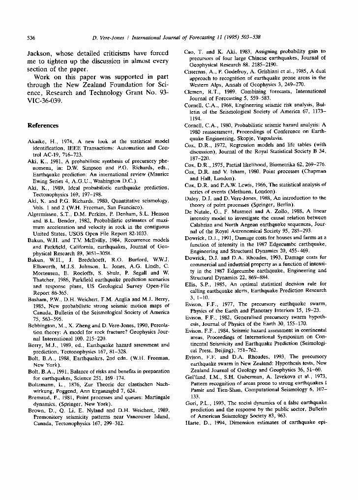
536 D. Vere-Jones / International Journal of Forecasting 11 (1995) 503-538
Jackson, whose detailed criticisms have forced me to tighten up the discussion in almost every section of the paper.
Work on this paper was supported in part through the New Zealand Foundation for Sci- ence, Research and Technology Grant No. 93- VIC-36-039.
References
Akaike, H., 1974, A new look at the statistical model identification, IEEE Transactions: Automation and Con- trol AC-19, 716-723.
Aki, K., 1981, A probabilistic synthesis of precursory phe- nomena, in: D.W. Simpson and P.G. Richards, eds., Earthquake prediction: An international review (Maurice Ewing Series 4, A.G.U., Washington D.C.).
Aki, K., 1989, Ideal probabilistic earthquake prediction, Tectonophysics 169, 197-198.
Aki, K. and P.G. Richards, 1980, Quantitative seismology, Vols. 1 and 2 (W.H. Freeman, San Francisco).
Algermissen, S.T., D.M. Perkins, P. Denham, S.L. Henson and B.L. Bender, 1982, Probabilistic estimates of maxi- mum acceleration and velocity in rock in the contiguous United States, USGS Open File Report 82-1033.
Bakun, W.H. and T.V. McEvilly, 1984, Recurrence models and Parkfield, California, earthquakes, Journal of Geo- physical Research 89, 3051-3058.
Bakun, W.H., J. Bredehoeft, R.O. Burford, W.W.J. Ellsworth, M.J.S. Johnson, L. Jones, A.G. Lindh, C. Mortensen, E. Roeloffs, S. Shulz, P. Segall and W. Thatcher, 1986, Parkfield earthquake prediction scenarios and response plans, US Geological Survey Open-File Report 86-365.
Basham, P.W., D.H. Weichert, F.M. Anglia and M.J. Berry, 1985, New probabilistic strong seismic motion maps of Canada, Bulletin of the Seismological Society of America 75, 563-595.
Bebbington, M., X. Zheng and D. Vere-Jones, 1990, Percola- tion theory: A model for rock fracture? Geophysics Jour- nal International 100, 215-220.
Berry, M.J., 1989, ed., Earthquake hazard assessment and prediction, Tectonophysics 167, 81-328.
Bolt, B.A., 1988, Earthquakes, 2nd edn. (W.H. Freeman, New York).
Bolt, B.A., 1991, Balance of risks and benefits in preparation for earthquakes, Science 251, 169-174.
Boltzmann, L., 1876, Zur Theorie der elastischen Nach- wirkung, Poggend, Ann Erganzsgbd 7, 624.
Bremaud, P., 1981, Point processes and queues: Martingale dynamics, (Springer, New York).
Brown, D., Q. Li, E. Nyland and D.H. Weichert, 1989, Premonitory seismicity patterns near Vancouver Island, Canada, Tectonophysics 167, 299-312.
Cao, T. and K. Aki, 1983, Assigning probability gain to precursors of four large Chinese earthquakes, Journal of Geophysical Research 88, 2185-2190.
Cisternas, A., P. Godefroy, A. Grishiani et al., 1985, A dual approach to recognition of earthquake prone areas in the Western Alps, Annals of Geophysics 3, 249-270.
Clemen, R.T., 1989, Combining forecasts, International Journal of Forecasting 5, 559-583.
Cornell, C.A., 1968, Engineering seismic risk analysis, Bul- letin of the Seismological Society of America 67, 1173- 1194.
Cornell, C.A., 1980, Probabilistic seismic hazard analysis: A 1980 reassessment, Proceedings of Conference on Earth- quake Engineering, Skopje, Yugoslavia.
Cox, D.R., 1972, Regression models and life tables (with discussion), Journal of the Royal Statistical Society B 34, 187-220.
Cox, D.R., 1975, Partial likelihood, Biometrika 62, 269-276. Cox, D.R. and V. Isham, 1980, Point processes (Chapman
and Hall, London). Cox, D.R. and P.A.W. Lewis, 1966, The statistical analysis of
series of events (Methuen, London). Daley, D.J. and D. Vere-Jones, 1988, An introduction to the
theory of point processes (Springer, Berlin). De Natale, G., F. Musmeci and A. Zollo, 1988, A linear
intensity model to investigate the causal relation between Calabrian and North Aegean earthquake sequences, Jour- nal of the Royal Astronomical Society 95, 285-293.
Dowrick, D.J., 1991, Damage costs for houses and farms as a function of intensity in the 1987 Edgecumbe earthquake, Engineering and Structural Dynamics 20, 455-469.
Dowrick, D.J. and D.A. Rhoades, 1993, Damage costs for commercial and industrial property as a function of intensi- ty in the 1987 Edgecumbe earthquake, Engineering and Structural Dynamics 22, 869-884.
Ellis, S.P., 1985, An optimal statistical decision rule for calling earthquake alerts, Earthquake Prediction Research 3, 1-10.
Evison, F.F., 1977, The precursory earthquake swarm, Physics of the Earth and Planetary Interiors 15, 19-23.
Evison, F.F., 1982, Generalised precursory swarm hypoth- esis, Journal of Physics of the Earth 30, 155-170.
Evison, F.F., 1984, Seismic hazard assessment in continental areas, Proceedings of International Symposium on Con- tinental Seismicity and Earthquake Prediction (Seimologi- cal Press, Beijing), 751-762.
Evison, F.F. and D.A. Rhoades, 1993, The precursory earthquake swarm in New Zealand: Hypothesis tests, New Zealand Journal of Geology and Geophysics 36, 51-60.
Gel'land, I.M., S.H. Guberman, A. Izvekova et al., 1973, Pattern recognition of areas prone to strong earthquakes I Pamir and Tien-Shan, Computational Seismology 6, 107- 133.
Gori, P.L., 1993, The social dynamics of a false earthquake prediction and the response by the public sector, Bulletin of American Seismology Society 83, 963.
Harte, D., 1994, Dimension estimates of earthquake epi-
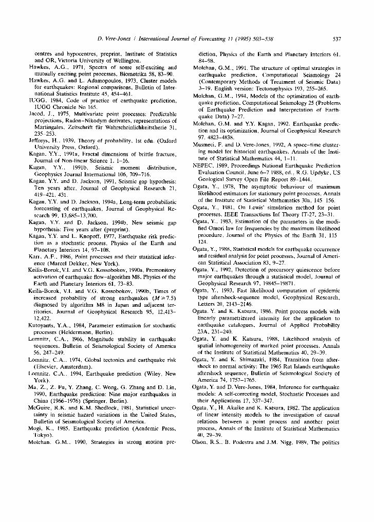
D. Vere-Jones / International Journal of Forecasting 11 (1995) 503-538 537
centres and hypocentres, preprint, Institute of Statistics and OR, Victoria University of Wellington.
Hawkes, A.G., 1971, Spectra of some self-exciting and mutually exciting point processes, Biometrika 58, 83-90.
Hawkes, A.G. and L. Adamopoulos, 1973, Cluster models for earthquakes: Regional comparisons, Bulletin of Inter- national Statistics Institute 45, 454-461.
IUGG, 1984, Code of practice of earthquake prediction, IUGG Chronicle No 165.
Jacod, J., 1975, Multivariate point processes: Predictable projections, Radon-Nikodym derivates, representations of Martingales, Zeitschrift f/Jr Wahrscheinlichkeitstherie 31, 235-253.
Jeffreys, H., 1939, Theory of probability, 1st edn. (Oxford University Press, Oxford).
Kagan, Y.Y., 1991a, Fractal dimensions of brittle fracture, Journal of Non-linear Science 1, 1-16.
Kagan, Y.Y., 1991b, Seismic moment distribution, Geophysics Journal International 106, 709-716.
Kagan, Y.Y. and D. Jackson, 1991, Seismic gap hypothesis: Ten years after, Journal of Geophysical Research 21, 419-421, 431.
Kagan, Y.Y. and D. Jackson, 1994a, Long-term probabilistic forecasting of earthquakes, Journal of Geophysical Re- search 99, 13,685-13,700.
Kagan, Y.Y. and D. Jackson, 1994b, New seismic gap hypothesis: Five years after (preprint).
Kagan, Y.Y. and L. Knopoff, 1977, Earthquake risk predic- tion as a stochastic process, Physics of the Earth and Planetary Interiors 14, 97-108.
Karr, A.F., 1986, Point processes and their statistical infer- ence (Marcel Dekker, New York).
Keilis-Borok,V.I. and V.G. Kossobokov, 1990a, Premonitory activation of earthquake flow-algorithm M8, Physics of the Earth and Planetary Interiors 61, 73-83.
Keilis-Borok, V.I. and V.G. Kossobokov, 1990b, Times of increased probability of strong earthquakes (M~>7.5) diagnosed by algorithm M8 in Japan and adjacent ter- ritories, Journal of Geophysical Research 95, 12,413- 12,422.
Kutoyants, Y.A., 1984,Parameter estimation for stochastic processes (Heldermann, Berlin).
Lomnitz, C.A., 1966, Magnitude stability in earthquake sequences, Bulletin of Seismological Society of America 56, 247-249.
Lomnitz, C.A., 1974, Global tectonics and earthquake risk (Elsevier, Amsterdam).
Lomnitz, C.A., 1994, Earthquake prediction (Wiley, New York).
Ma, Z., Z. Fu, Y. Zhang, C. Wong, G. Zhang and D. Lin, 1990, Earthquake prediction: Nine major earthquakes in China (1966-1976) (Springer, Berlin).
McGuire, R.K. and K.M. Shedlock, 1981, Statistical uncer- tainty in seismic hazard variations in the United States, Bulletin of Seismological Society of America.
Mogi, K., 1985, Earthquake prediction (Academic Press, Tokyo).
Molchan, G.M., 1990, Strategies in strong motion pre-
diction, Physics of the Earth and Planetary Interiors 61, 84-98.
Molchan, G.M., 1991, The structure of optimal strategies in earthquake prediction, Computational Seismology 24 (Contemporary Methods of Treatment of Seismic Data) 3-19. English version: Tectonophysics 193, 255-265.
Molchan, G.M., 1994, Models of the optimization of earth- quake prediction, Computational Seismology 25 (Problems of Earthquake Prediction and Interpretation of Earth- quake Data) 7-27.
Molchan, G.M. and Y.Y. Kagan, 1992, Earthquake predic- tion and its optimization, Journal of Geophysical Research 97, 4823-4838.
Musmeci, F. and D. Vere-Jones, 1992, A space-time cluster- ing model for historical earthquakes, Annals of the Insti- tute of Statistical Mathematics 44, 1-1 I.
NEPEC, 1989, Proceedings National Earthquake Prediction Evaluation Council, June 6-7 1988, ed., R.G. Updyke, US Geological Survey Open File Report 89-1444.
Ogata, Y., 1978, The asymptotic behaviour of maximum likelihood estimators for stationary point processes, Annals of the Institute of Statistical Mathematics 30a, 145-156.
Ogata, Y., 1981, On Lewis' simulation method for point processes, IEEE Transactions Inf Theory IT-27, 23-31.
Ogata, Y., 1983, Estimation of the parameters in the modi- fied Omori law for frequencies by the maximum likelihood procedure, Journal of the Physics of the Earth 31, 115- 124.
Ogata, Y., 1988, Statistical models for earthquake occurrence and residual analysis for point processes, Journal of Ameri- can Statistical Association 83, 9-27.
Ogata, Y., 1992, Detection of precursory quiescence before major earthquakes through a statistical model, Journal of Geophysical Research 97, 19845-19871.
Ogata, Y., 1993, Fast likelihood computation of epidemic type aftershock-sequence model, Geophysical Research, Letters 20, 2143-2146.
Ogata, Y. and K. Katsura, 1986, Point process models with linearly parametrizered intensity for the application to earthquake catalogues, Journal of Applied Probability 23A, 231-240.
Ogata, Y. and K. Katsura, 1988, Likelihood analysis of spatial inhomogeneity of marked point processes, Annals of the Institute of Statistical Mathematics 40, 29-39.
Ogata, Y. and K. Shimazaki, 1984, Transition from after- shock to normal activity: The 1965 Rat Islands earthquake aftershock sequence, Bulletin of Seismological Society of America 74, 1757-1765.
Ogata, Y. and D. Vere-Jones, 1984, Inference for earthquake models: A self-correcting model, Stochastic Processes and their Applications 17, 337-347.
Ogata, Y., H. Akaike and K. Katsura, 1982, The application of linear intensity models to the investigation of causal relations between a point process and another point process, Annals of the Institute of Statistical Mathematics 40, 29-39.
Olson, R.S., B. Podestra and J.M. Nigg, 1989, The politics

538 D. Vere-Jones / International Journal of Forecasting 11 (1995) 503-538
of earthquake prediction (Princeton University Press, Princeton).
Omori, T., 1894, On the aftershocks of earthquakes, Journal of the College of Science of the Imperial University of Tokyo 7, 111-200.
Rathbun, S.I., 1993, Modelling marked spatio-temporal point patterns, Bulletin of International Statistics Institute (Proceedings 49th Session of ISI), Vol. 2, 379-396.
Rauch, E. and A. Smolka, 1992, Earthquake insurance: Seismic exposure and portfolio dispersal; their influence on the probable maximum loss, Earthquake Engineering 10th World Conference, Balkema, Rotterdam, 6101-6104.
Reid, H.F., 1910, The mechanics of earthquakes, University of California Publication, Bulletin of the Department of Geological Sciences 6, 413-433.
Rhoades, D.A., 1989, Independence, precursors and earth- quake hazard, Tectonophysics 169, 199-206.
Rhoades, D.A. and F.F. Evison, 1979, Long-range earth- quake forecasting based on a single precursor, Geophysics, Journal of Royal Astronomical Society 59, 43-56.
Rhoades, D.A. and F.F. Evison, 1989, Time variable factors in earthquake hazard, Tectonophysics 167, 201-210.
Rhoades, D.A. and F.F. Evison, 1993, Long-range forecast- ing based on a single precursor with clustering, Geo- physical Journal International 113, 371-381.
Rikitake, T., 1976, Earthquake prediction (Elsevier, Am- sterdam).
Ripley, B., 1988, Statistical inference for spatial processes (Cambridge University Press, Cambridge).
Sakamoto, Y., M. Ishiguro and G. Kitagawa, 1983, Akaike information criterion statistics (Reidel, Dordrecht).
Schwartz and Coppersmith, 1984, Fault behaviour and characteristic earthquakes: Examples from the Wasatch and San Andreas Faults, Journal of Geophysical Research 89, 5681-5698.
Sieh, K., 1981, A review of geological evidence for recur- rence times of large earthquakes, in: D. Simpson and P. Richards, eds., Earthquake prediction, an international review (MEwing Series 8, American Geophysical Union) 209-216.
Silverman, B., 1986, Density estimation for statistics and data analysis (Chapman and Hall, London).
Snyder, D.L., 1975, Random point processes (Wiley, New York).
Stoyan, D., W.S. Kendall and J. Mecke, 1987, Stochastic geometry and its applications (Springer, Berlin).
UNEP, 1980, Report of expert group meeting, Nairobi, Document Working Group B3,5.
Utsu, T., 1979, Calculation of the probability of success of an earthquake prediction (in the case of the Izu-Oshima- Kinkai earthquake of 1978), Report of Coordinating Committee for Earthquake Prediction, 164-166.
Utsu, T., 1983, Probabilities associated with earthquake prediction and their relationship, Earthquake Prediction Research, 105-114.
Veneziano, D. and J. Van Dyck, 1987, Statistical analysis of earthquake catalogues for seismic hazard, in: Y.K. Lin and R. Minoi, eds., Stochastic applications in earthquake engineering, Lecture notes in engineering 32 (Springer, Berlin) 385-427.
Vere-Jones, D., 1970, Stochastic models for earthquake occurrence (with discussion), Journal of Royal Statistical Society B 32, 1-62.
Vere-Jones, D., 1976, A branching model for crack propaga- tion, Pure Applied Geophysics 114, 711-726.
Vere-Jones, D., 1977, Statistical theories for crack propaga- tion, Mathematical Geology 9, 455-481.
Vere-Jones, D., 1978, Earthquake prediction: A statistician's view, Journal of the Physics of the Earth 26, 129-146.
Vere-Jones, D., 1983, What are the main uncertainties in estimating earthquake risk? Bulletin of New Zealand National Society for Earthquake Engineering 16(1), 39- 44.
Vere-Jones, D., 1988, Statistical aspects of the analysis of historical earthquake catalogues, in: C. Margottini, ed., Historical seismicity of Central-Eastern Mediterranean region (ENEA, Rome) 271-297.
Vere-Jones, D., 1992, Statistical methods for the description and display of earthquake catalogues, in: A.T. Walden and P. Guttorp, eds., Statistics in the environmental and earth sciences (Edward Arnold, London) 220-246.
Vere-Jones, D. and Y. Deng, 1988, A point process analysis of historical earthquakes from North China, Earthquake Research in China (English translation) 2(2), 165-181.
Vere-Jones, D. and T. Ozaki, 1982, Some examples of statistical estimation applied to point process data, 1 Cyclic Poisson and self-exciting models, Ann Inst Stat Math 34 B, 189-207.
Wang, A.L., D. Vere-Jones and X. Zheng, 1991, Simulation and estimation procedures for stress release models, in: M.J. Beckmann, M.N. Gopalan and R. Subramanian, eds., Stochastic processes and their applications, Lecture notes in economics and mathematical systems 370 (Spring- er, Berlin) 11-27.
Working Group on Californian Earthquake Probabilities, 1988, Probabilities of large earthquakes occurring in Cali- fornia on the San Andreas Fault, US Geological Survey Open File Report 88-398.
Working Group on Californian Probabilities, 1990, Prob- abilities of earthquakes in the San Francisco Bay region, California, US Geological Survey Circular 1053.
Zheng, X. and D. Vere-Jones, 1991, Application of stress release models to historical earthquakes from North China, Pure Applied Geophysics 135, 559-576.
Zheng, X. and D. Vere-Jones, 1994, Further applications of the stress release model to historical earthquake data, Tectonophysics 229, 101-121.