Applied Energy 193 (2017) 287–296

Contents lists available at ScienceDirect

Applied Energy

journal homepage: www.elsevier .com/locate /apenergy

Forecasting electricity demand for Turkey: Modeling periodic variationsand demand segregation

http://dx.doi.org/10.1016/j.apenergy.2017.02.0540306-2619/� 2017 Elsevier Ltd. All rights reserved.

⇑ Corresponding author.E-mail address: ahmety@khas.edu.tr (A. Yucekaya).

Ergun Yukseltan a, Ahmet Yucekaya b,⇑, Ayse Humeyra Bilge a

aGraduate School of Science & Engineering, Kadir Has University, Istanbul, Turkeyb Industrial Engineering Department, Kadir Has University, Istanbul, Turkey

h i g h l i g h t s

� We include the modulation of daily and weekly variations by seasonal harmonics.� We forecast demand without physical parameters involved.� We forecasted the demand 1-week and 1-day horizons with %3 MAPE.� We propose a method to estimate the share of industrial electricity in total demand.� We use special days, holidays and exceptional events to segregate demand.

a r t i c l e i n f o

Article history:Received 29 September 2016Received in revised form 3 February 2017Accepted 18 February 2017Available online 24 February 2017

Keywords:Time series analysisFourier seriesElectricity demand for TurkeyDemand segregationLoad forecast

a b s t r a c t

In deregulated electricity markets the independent system operator (ISO) oversees the power system andmanages the supply and demand balancing process. In a typical day the ISO announces the electricitydemand forecast for the next day and gives participants an option to prepare offers to meet the demand.In order to have a reliable power system and successful market operation, it is crucial to estimate theelectricity demand accurately. In this paper, we develop an hourly demand forecasting method on annual,weekly and daily horizons, using a linear model that takes into account the harmonics of these variationsand the modulation of diurnal periodic variations by seasonal variations. The electricity demand exhibitscyclic behavior with different seasonal characteristics. Our model is based solely on sinusoidal variationsand predicts hourly variations, without using any climatic or econometric information. The method isapplied to the Turkish power market on data for the period 2012–2014 and predicts the demand overdaily and weekly horizons within a 3% error margin in the Mean Absolute Percentage Error (MAPE) norm.We also discuss the week day/weekend/holiday consumption profiles to infer the proportion of industrialand domestic electricity consumption.

� 2017 Elsevier Ltd. All rights reserved.

1. Introduction

‘‘Poolco” is one of the main market competition structures usedin deregulated markets [1]. Trading platforms such as the‘‘day-ahead market”, ‘‘balancing market” and ‘‘intra-day market”are developed to increase the functionality and success of themarket mechanism.

The demand forecast has always played an important role incapacity and transmission planning, generation scheduling andpricing. However, the deregulation and privatization of the powermarkets increased the importance of demand or load forecastingsince the success of the markets is highly related to their accuracy.

The demand forecast has different aspects at different forecasthorizons. For example, for capacity planning one needs a long termforecast of aggregate demand as a function of economic or demo-graphic parameters. On the other hand, short term (hourly) fore-casts are essential for the efficiency of day-ahead markets. Shortterm variations have a ‘‘regular” component depending on dailyroutines and seasonal effects. Exceptional conditions (extremeweather conditions) and exceptional events (holidays, sportsevents) cause ‘‘irregular” variations that affect and modify this pat-tern. It is an interesting and challenging problem to forecast the‘‘regular” component of the hourly demand for the planning ofthe day-ahead market over a long term i.e., year-long horizon.The model that we develop in this paper is based solely onsinusoidal variations and predicts hourly variations over a 1-yearhorizon, within a 3% Mean Absolute Percentage Error (MAPE),

288 E. Yukseltan et al. / Applied Energy 193 (2017) 287–296

without using any climatic or econometric information. The incor-poration of the irregular variations to this model will be the subjectof ongoing work. These irregular variations fall into ‘‘predictable”and ‘‘unpredictable” categories. The predictable variations arechanges in the demand patterns that are tied to predictable naturalor social events and they can be included in the basic model as anew set of regressors. Unpredictable irregular variations arechanges in the demand that are of yet unknown origin and theyhave to be treated with special methods, such as the ‘‘feedback”method used in Bilge and Tulunay [2] or time series and stochasticapproaches reviewed below.

In the literature, descriptions and comparisons of various fore-cast methods have been presented by a number of researchers. Lin-ear models, Time Series Methods such as ARMA and ARIMA,statistical models and other numerical methods like Artificial Neu-ral Networks (ANN), Genetic Algorithms (GA), Support VectorMachines (SVM) and Particle Swarm Optimization are commonapproaches that are used for electric demand forecasting.

Dyner and Larsen present an analysis for the liberalization ofelectricity markets and discuss the usability of ‘‘agent modeling”,‘‘simulation”, ‘‘game theory” and ‘‘risk management” for takinginto account stochastic characteristics of load and demand [3].Anand and Suganthi present a review of energy demand forecast-ing models, discussing traditional methods such as ‘‘time series”,‘‘regression”, ARIMA and new methods such as ‘‘Support VectorMachines”, ‘‘Ant Colony” and ‘‘Particle Swarm Optimization” [4].Hahn et al. present a survey of electricity load forecasting methodsand tools for decision making [5]. Conejo et al. compare ‘‘timeseries analysis”, ‘‘neural networks” and ‘‘wavelets” for electricitydemand forecasting in the market. They conclude that time seriesmethods provide more accurate results for short term forecasting[6].

Regression methods that are quite convenient and easy toimplement have been applied widely for electricity demand fore-casting. Vilar et al. use a ‘‘nonparametric regression” technique toforecast the next-day electricity demand and price with a semi-functional partial linear model. Their model is applied to Spanishdata and the results are compared with that of ‘‘naïve” and‘‘ARIMA” methods [7]. Taylor uses statistical forecasting methodsfor short term electricity demand forecasting. He extends the threedouble seasonal methods in order to accommodate the intra-yearseasonal cycle and applies the method to six years of British andFrench data [8]. Clements et al., show that a multiple equationtime-series model can forecast the load as accurately as complexnonlinear and nonparametric forecasting models. They apply themethod to Australian data and they reach a very low MAPE usingan 11-year data set [9]. Fan and Hyndman propose ‘‘semi-parametric additive models” to estimate the relationships betweendemand and inputs such as calendar variables, lagged actualdemand observations, and historical and forecast temperature.Their method is applied to the Australian National ElectricityMarket to forecast half-hour electricity demand for up to one week[10]. Wang et al. use the ‘‘PSO optimal Fourier method”, the‘‘seasonal ARIMA” model and apply their combinations to theNorthwest electricity grid of China for correcting the forecastingresults of seasonal ARIMA. Their results show that the predictionaccuracy of the combined models is higher than that of the singleseasonal ARIMA [11,12]. A ‘‘semi-parametric additive regression”model is proposed to estimate the relationships between demandand temperatures, calendar effects and some demographic andeconomic variables in Hyndman and Fan [10], Fan and Hyndman[13]. Hyndman and Fan then calculate the density forecasts andfull probability distributions of the possible future values of thedemand while also considering the holidays and weekends. Asimilar regression approach is proposed in McSharry et al. [14] toanalyze the relationship between demand and other variables.

The author uses five different exponential smoothing methods toapply the methodology to British and French half-hourly load datain Taylor [15].

The application of time series methods to the forecast of theelectricity demand is also popular in the literature. ‘‘ARIMA” is pre-ferred mostly for short and long term electricity demand. Futuredemand is predicted using an ARIMA model and profit functionis developed as an objective in Niu et al. [16]. Andersen et al. pro-pose an econometric modeling approach for the long term fore-casting of hourly electric consumption in local areas. Data fromthe Danish market is used for the analysis and the estimated loadprofiles are used by the transmission operator [17]. Lo and Wuexamine local forecast uncertainty: Artificial Neural Networksand ARIMA models are used to calculate the load, highlight highrisk in different periods and evaluate daily value at risk [18]. InChakhchoukh et al. [19] the authors use statistical analysis meth-ods to forecast the short term demand. They compare these meth-ods with classical models like ARIMA and show that the proposedmethod can outperform the classical ones. The authors develop amultiple linear regression model based on calendar and weatherrelated variables to analyze the relationship between meteorolog-ical variables and monthly electricity demand. The method isapplied to forecast the electricity demand in Italy and returnspromising results [20].

In addition to the basic approaches cited above, based on theproblem scope and objective, a number of alternative methodsare also proposed in the literature. Zhang and Dong use an ‘‘artifi-cial neural network” model and wavelet transformed data togetherto forecast electricity demand for short periods [21]. Heuristicapproaches such as ‘‘particle swarm optimization”, ‘‘evolutionalgorithms” or hybrid approaches are also used to forecast the elec-tricity demand [22,11,12,23]. Azadeh et al. use ‘‘neural networks”and ‘‘genetic algorithms” to predict the electrical energy consump-tion using economic indicators such as price, value added, numberof customers and consumption in previous periods. The integratedGA and ANN method returns less (MAPE) when applied to theIranian electricity market [24]. Pai and Hong propose a methodto forecast the electricity load using recurrent Support VectorMachines (SVM) with Genetic Algorithms. They use electricity datafrom Taiwan and they show that the proposed method outper-forms the SVM, neural network and regression models [25]. Wangand Ramsay develop a ‘‘neural network” based estimation for elec-tricity spot prices, focusing particularly on weekends and publicholidays [26]. A similar approach for electricity demand forecast-ing with a focus on weekends and public holidays is given inSrinivasan et al. [27].

It is true that the temperature and climate can affect electricitydemand, and hence, can be included in the forecasting model. Theeffect of weather on electricity consumption is studied by Taylorand Buizz, who use weather conditions to forecast short term elec-tricity demand for 1–10 days ahead. Various weather scenarios areincluded in their models and it is shown that the model thatincludes weather scenarios returns more accurate results for theshort term than the traditional weather forecasts [28]. Feliceet al. use statistical modeling to analyze the influence of tempera-ture on load forecasting in Italy both at the national and regionallevel using unprecedented historical load data [29].

In Crowley and Joutz [30] the authors show that electricity con-sumption due to increased cooling needs continues even after thehigh temperatures return to normal due to the heat capacity of thebuildings. This shows that the effects of weather conditions onelectricity consumption is far from being simple. This is also toshow that approaches that can capture the demand patternwithout using physical parameters might return better forecasts,as we present in this research. Table 1 provides an overview ofmethods and resources.

Table 1Overview of the forecasting methods and related resources.

Methods Sources

Time series analysis [10,4,9,16–18]Statistical methods [7,8,10–15,19,20]Surveys [3–5,10]artificial neural network and simulation [21,26,27],Heuristic approaches [11,12,22–25]Temperature based methods [28–30]

E. Yukseltan et al. / Applied Energy 193 (2017) 287–296 289

In our case, inclusion of the deviations from comfortable tem-peratures (heating degree day) and (cooling degree day) broughtonly a minor improvement to the model, possibly because themodulation regressors had already taken into account the effectsof temperature.

As discussed in the following chapters, we also see that irregu-lar holidays or special days have a strong impact on the electricitydemand. The effect of holidays on electric power demand andprices has always been a topic of interest. The power companiesuse time of pricing tariffs for holidays and develop generationand transmission plans considering holiday effects [31,32],. Theeffect of irregular holidays on electricity demand is taken intoaccount by Braubacher and Wilson in their model for hourly elec-tricity demand, where they replace the data for the holidays withan interpolation of demand for the before and after holiday periods[33].

In this paper, we develop a linear model, as an expansion inFourier series supplemented with a modulation by seasonal har-monics, in which the workdays and weekends form two nearlyindependent sets of variations. The model includes harmonics ofdaily, weekly and seasonal variations and a linear term to take intoaccount the trends. The novelty of the model is the inclusion of themodulation of the high frequency harmonics (daily and weeklyvariations) by low frequency harmonics (seasonal variations). Themethod is completely generic and applicable to any load forecast-ing problem characterized by daily, weekly, and seasonal periods.The model may be supplemented by regressors such as time seriesfor physical parameters (temperature and/or humidity in thiscase). However, the inclusion of such regressors added only aminor improvement to the results and they were omitted in thepresent model. We may thus claim that the modulation of diurnalvariations by seasonal harmonics captures the essence of the sea-sonal effects in electricity demand. The daily variation patternsthat play a crucial role reflect habits that are usually common tomost countries, as work hours and off times are quite similar.

The model can be replicated for any country as it captures peri-odic variations based on the historical demand data only. Local fea-tures of the analysis are the regional and religious holidays. Wetook advantage of these features for demand segregation, but weinterpolated data for these periods, hence we ignored them for pre-diction and forecast. A similar approach can be adopted in theapplication of the model to any other country. The next local fea-ture is the weekday-weekend structure, which is taken intoaccount by introducing harmonics of 7 days in the model. In Tur-key, the weekend structure is the same as the European zone,but the model works for any country that has a 2 day weekendstarting at a different day or even in countries with a 1 day week-end. Applying the model to the Turkish Power market, we wereable to model and predict demand within 3% MAPE over a wholeyear without any climatic information. Here and in any other coun-try, local features such as the low and high demand periods such asfor national holidays, elections and competitions could be includedin the model to make a better analysis.

In Section 2, we present an overview of the Turkish Power mar-ket, the data used for the validation of the model and a discussionof the structure of the daily variation curves and the effect ofexceptional events. In Section 3 we present a linear regressionmodel using low and high frequency harmonics and their interac-tion as modulated waves. In Section 4 we use various schemes forthe forecasting of the demand and we present our forecast resultsfor annual, weekly and daily demand within about 3% MAPE. InSection 5, we discuss predictions using these models to estimatethe proportion of industrial versus household electricity demand.In Sections 6 and 7, we present the conclusion and suggestionsfor future directions respectively.

2. Data processing and the Turkish power market

In Turkey, the electric power market used to be state owned andcontrolled in generation, transmission and distribution until thebeginning of the 2000s. The market design started in 2003 bytransferring state monopoly rights to private companies for gener-ation, transmission and distribution and by privatizing energyassets. The balance and conciliation phase was launched in 2006and the participants carried out bidding and bilateral contractsuntil the end of 2009. The day-ahead planning was built in thisyear; as a result of the market’s development, the day-ahead plan-ning was converted to the day-ahead market in 2011. After suc-cessfully implementing the day-ahead market, the systemoperator established the intra-day market in 2014 under the con-trol of the new market operator, the Market Financial SettlementCentre System (EPIAS).

The main goal of the day-ahead market is to increase the plan-ning accuracy and reliability of the power system on an hourlybasis. In the day-ahead market, the system operator announcesthe estimated day-ahead demand for each hour of the next day.The two parties can determine the power price and delivery condi-tions and they can have independent bilateral contracts. The totalamount of power that will be provided with the bilateral contractsis determined and deducted from the total day ahead demand.Then the remaining power is open to the market to be suppliedby competitive and reliable bids. The suppliers submit their hourlycapacities and respective prices for the next day as a response tohourly demand forecasts that are announced by EPIAS. This processis called ‘‘bidding into market”. Having details of generation capac-ities and price offers, the system operator sorts these on a meritbased system. The algorithm stops where the cumulative genera-tion capacities meet the forecasted hourly demand and the day-ahead price for that hour is determined. This price is accepted asthe ‘‘marginal price” and announced as the ‘‘system day-aheadprice” for that hour. The process is repeated for 24-h and partici-pants are informed of the final day-ahead generation schedulesand market prices.

The generation and demand of electricity possess stochastic fea-tures making them hard to estimate accurately in a typical day. The‘‘balancing market (real time market)” is planned to manage suchunexpected circumstances in both demand and generation. It isalso possible that a market participant needs to adjust its supplyand/or demand offer during a day. The ‘‘intra-day market” isdesigned for the participants who need to balance their contractualundertakings, generation or consumption plans. Another objectiveof the intra-day market is to decrease the imbalance in the systemand to provide an alternative electricity purchase/sale option forthe market participants. Hence, companies are able to provideadditional generation capacity or decrease their excess generationfor every hour.

The hourly demand data for the whole country is provided bythe system operator in the EPIAS system. The data includes market

290 E. Yukseltan et al. / Applied Energy 193 (2017) 287–296

prices, hourly imbalances and other related information withoutany demand or region segregation. We used data for the years2012–2014 and we modeled the ‘‘finalized generation plan”section of this data.

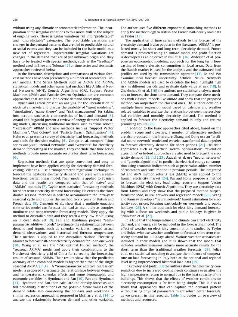
In Fig. 1, we present an overview of the data for the years 2012–2014, after correcting for switching to daylight saving time. In thesefigures, the low-demand periods correspond to two religious holi-days of durations 3 and 4 days respectively. These holidays aredetermined according to the lunar calendar and they are shiftedback by 10 days each year. In day ahead forecasts using modulated

Jul.10 Jul.15 Jul.20

× 104

1.5

2

2.5

3

3.5Weekly Demand P

Nov.27 Dec.02 Dec.07

× 104

1.5

2

2.5

3

3.5Weekly Demand P

Fig. 2. Typical hourly demand data, for w

0 1000 2000 3000 4000

× 104

0

2

42012

0 1000 2000 3000 4000

× 104

0

2

42013

0 1000 2000 3000 4000

× 104

0

2

42014

Fig. 1. Overview of the data after adjustment for daylight saving ti

Fourier expansions, these days will be treated as exceptional eventsand they will be replaced by appropriate averages. On the otherhand, the demand data for these periods will be used for estimatingthe share of household and industrial electricity consumption,because it is known that most factories stop working in these days.

In Fig. 2 we present typical 4-week periods in winter and insummer, where we see that not only the amplitude but also theshape of the periodic variations for weekdays, weekends, summerand winter are different. For example, the intraday peak shifts tothe afternoon in winter.

Jul.25 Jul.30 Aug.04

attern (Summer)

Dec.12 Dec.17 Dec.22

attern (Winter)

inter and summer for the year 2002.

5000 6000 7000 8000 9000

5000 6000 7000 8000 9000

5000 6000 7000 8000 9000

me. The low demand periods correspond to religious holidays.

× 104

1

2

3

4

Monday

× 104

1

2

3

4

Tuesday

× 104

1

2

3

4

Wednesday

× 104

1

2

3

4

Thursday× 104

1

2

3

4

Friday× 104

1

2

3

4

Saturday

0 10 20 0 10 20 0 10 20

0 10 20 0 10 20 0 10 20

0 10 20

× 104

1

2

3

4

Sunday

Fig. 3. Daily variation curves for electricity demand in the year 2012.

E. Yukseltan et al. / Applied Energy 193 (2017) 287–296 291

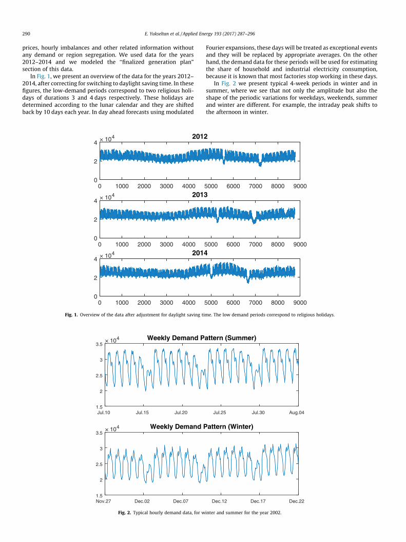
Fig. 3 shows the demand patterns for each day of the week forthe year 2012. We note that except for Sunday, the curves havesimilar shapes. The demand profile for Saturday is similar to week-days but it has lower amplitude. The days that have significantlylower demand correspond to January 1st and to the religious hol-idays as the demand decreases on these days. Moreover, the max-imum demand values for graphs of Saturdays and Fridayscorrespond to the fourth week of July, which were the warmestdays in 2012. In fact, this week’s temperature was recorded asthe warmest week since 1927 showing the effect of the tempera-ture on the demand.

This preliminary analysis shows the importance of knowledgeof local characteristics on the demand pattern. The work habitsand work hours are usually similar throughout the world. Thelength of the days is different though. Once the demand patternis identified and historical demand data is used, the model canbe successfully replicated.

3. Modeling of periodic variations

A glance at the data as displayed in Figs. 1 and 2, shows thatweekdays and weekends seem to form two independent sets ofvariations. At all times, diurnal variations are superimposed onseasonal variations, furthermore, diurnal variations have higheramplitudes in winter and in summer. In this section, we modelthe weekend effects and the modulation by seasonal variationsusing a standard linear regression model. The regressors are hourlysamples of sinusoidal functions expressed as column vectors[34,35],. We denote the harmonics of sinusoidal functions withperiods of 1 year (365 � 24 h), 1 week (7 � 24 h) and 1 day (24 h)respectively by Xi, Zk, and Yj. The modulation of the high frequencyvariations (Yj) by the low frequency variation (Xi) is included bythe component wise product of the corresponding vectors, denotedas XiYj respectively. The hourly electricity demand is denoted by S.These regressors are arranged as the columns of a matrix F, and thecoefficient vector a and model vector y are calculated as below.

F ¼ ½XiZkYj XiYj� ð1Þ

a ¼ ðFtFÞ�1FtS ð2Þ

y ¼ Fa ð3ÞA linear trend is also added as a regressor but as its effect is

minor it is not shown above. The model includes harmonics ofsinusoidal variations of periods of 24 h (Yi), 24 � 7 h (Zi) and24 � 365 h (Xi). The sampling theorem that states that the highestfrequency that can be recovered from data sampled at Dt timeintervals has period 2Dt, limits the harmonics Yi to sinusoidal func-tions with periods 24, 24/2 = 12, 24/3 = 8, . . .24/12 = 2 h. The num-ber of regressors should be large enough to capture the mainfeatures of the data but over-specification should be avoided. Thenumber of harmonics of the weekly and annual variations are cho-sen by this rule. The model uses 96 time regressors and 160 mod-ulation regressors. The detailed formulations are given in theAppendix.

The ‘‘modeling error” is measured by the ‘‘Mean Square Error(MSE)” and ‘‘Minimum Absolute Percentage Error (MAPE)”. If Shand yh are the actual demand and the forecasted demand for hourh, they are defined as:

MSE ¼ 1N

XN

h¼1

ðyh � ShÞ2 ð4Þ

MAPE ¼ 100N

XN

h¼1

jyh � ShjSh

ð5Þ

where N is the total number of data items. In Fig. 4 we present theresults of the proposed model in terms of the harmonics ofthe annual, diurnal and weekly variations and the modulation ofthe diurnal and weekly variations by seasonal harmonics for theyear 2012. This model is quite satisfactory and shows the powerof including modulation of the high frequency components by the

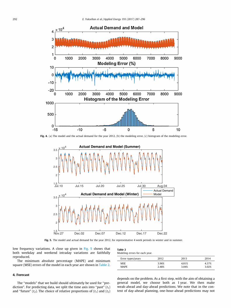
Fig. 4. (a) The model and the actual demand for the year 2012, (b) the modeling error, (c) histogram of the modeling error.

× 104

1.5

2

2.5

3

3.5Actual Demand and Model (Summer)

Actual DemandModel

Jul.10 Jul.15 Jul.20 Jul.25 Jul.30 Aug.04

Nov.27 Dec.02 Dec.07 Dec.12 Dec.17 Dec.22

× 104

1.5

2

2.5

3

3.5Actual Demand and Model (Winter)

Fig. 5. The model and actual demand for the year 2012, for representative 4 week periods in winter and in summer.

Table 2Modeling errors for each year.

Error types/years 2012 2013 2014

MSE 3.96% 4.81% 4.37%MAPE 2.48% 3.04% 3.02%

292 E. Yukseltan et al. / Applied Energy 193 (2017) 287–296

low frequency variations. A close up given in Fig. 5 shows thatboth weekday and weekend intraday variations are faithfullyreproduced.

The minimum absolute percentage (MAPE) and minimumsquare (MSE) errors of the model in each year are shown in Table 2.

4. Forecast

The ‘‘models” that we build should ultimately be used for ‘‘pre-diction”. For predicting data, we split the time axis into ‘‘past” (t1)and ‘‘future” (t2). The choice of relative proportions of (t1) and (t2)

depends on the problem. As a first step, with the aim of obtaining ageneral model, we choose both as 1 year. We then makeweak-ahead and day-ahead predictions. We note that in the con-text of day-ahead planning, one-hour-ahead predictions may not

E. Yukseltan et al. / Applied Energy 193 (2017) 287–296 293

be meaningful. On the other hand, they are needed for the intra-day market.

Once we choose the splitting of the time axis into past andfuture, we have a corresponding splitting of the matrix F, into F1,F2. In our model the regressors that are harmonics of annual, diur-nal and weekly variations are the same in F1 and F2.

In order to make a prediction, we use F1 to compute the coeffi-cient vector a but we use F2 to compute the model vector y2;

Table 3New modelling and annual prediction errors after adjustments.

Error types/years 2012 2013 2014 2014 annual prediction

MSE 1.85% 2.83% 2.81% 4.75%MAPE 1.34% 1.94% 2.12% 3.59%

Week0 10 20 30 40 50 60

MA

PE

1

2

3

4

5

6

7

8Week Ahead Forecast Errors

ActualDST adjusted

Fig. 6. Week-ahead forecast error ratios for actual and data shifted to correct thedaylight savings time.

× 104

1.5

2

2.5

3

3.5Forecast with Actu

0 20 40 60 80

0 20 40 60 80

× 104

1.5

2

2.5

3

3.5Forecast with Shift

Fig. 7. Time domain plots of the original data and forecast for week 45 of the year 2014 (u

a1 ¼ ðFt1F1Þ�1

Ft1S1; y2 ¼ F2a1 ð6Þ

The prediction error of MSE and MAPE norms are based on thedifference S2-y2. Usually the prediction error is larger than themodeling error. We test the forecast accuracy of the models forthe annual, weekly and daily forecast periods in the followingsections.

4.1. Annual forecast

The forecast error for the year 2014, which is found using thedemand data for 2013, is around 9% which is not satisfactory com-pared to the modeling error [34]. These high prediction error per-centages are tied to the time shift of the religious holidays and tothe phase shift of the weekday-weekend structure when workingon an annual basis. In order to cure the phase differences, we con-sidered 3-year data as a concatenation of 52 week periods. Then,we corrected for the demand during the religious holidays andthe first day of the year by using the average demands for the nextand the previous weeks. With these adjustments, both the model-ing and the prediction errors improved considerably as shownbelow in Table 3.

4.2. Week-ahead forecast

In this section we use a 2-year (104 weeks) observation periodto predict next-week’s hourly demand and repeat this for 52 con-secutive weeks. This sliding window approach provides a dynamicforecast model by considering recent past period demand habitsand events. Fig. 6 shows an overview of the week-ahead errorratios.

In the plot of the prediction errors we see that the predictionerrors are higher for the period right after switching back fromthe daylight savings time in October. This effect can be seen clearlyin the graphs. We have re-run the model after shifting data to takeinto account the switching from daylight savings time. As shown inFigs. 6 and 7, this process improves the forecast results. As shown

al Data (Week 45)

100 120 140 160 180

100 120 140 160 180

ed Data (Week 45)

pper panel original data and lower panel after correcting for daylight savings time).

294 E. Yukseltan et al. / Applied Energy 193 (2017) 287–296

in Fig. 7, the left and right panels correspond to original and shifteddata respectively.

4.3. Day-ahead forecast

For day-ahead forecasts, we applied the same method to a two-year period. Only the roll-over period changed from week to day.Similarly, day-ahead forecast results improved with shifting dataafter the daylight saving time ended in October as shown in Fig. 8.

Deviations from comfortable temperatures is known to affectelectricity demand [28]. We clearly observed this effect when weobserved that maximum demand occurs in the week with thewarmest temperatures as shown in Section 2. We incorporateddeviations from comfortable temperatures in our model but thisresulted only in a minor improvement on the forecast. This mightbe due to the fact that modulation by seasonal harmonics modelstemperature effects adequately as the modulated Fourier expan-sion is used.

Day0 50 100 150 200 250 300 350 400

MA

PE

0

2

4

6

8

10

12

14

16

18Day Ahead Forecast Errors

ActualDST adjusted

Fig. 8. Day-ahead error ratios for actual and shifted data.

Table 4Forecast results in Model 2.

Error MSE MAPE

Daily roll-over 3.52% 3.06%Daily roll-over(phase adjusted) 3.24% 2.86%Weekly roll over 3.95% 3.27%Weekly roll-over(phase adjusted) 3.65% 3.05%Weekly roll-over(temperature added) 3.41% 3.04%

Fig. 9. Moving average values for two wee

On the other hand, as seen in Table 4, with phase adjustment,we obtained considerable improvements in the accuracy of fore-casting. When we checked all of the results, we see that the day-ahead forecast is the most accurate. This proves the power of themodel in short term demand prediction.

Moreover, as we highlighted before, daily demand is affected byexceptional events. In order to increase forecast accuracy, we needto input more information about exceptional events such as hightemperatures, the world cup, and elections that cause changes indaily life routines.

5. Demand segregation

In this section we focus on estimating the share of industrialand residential demand from the total demand data. As observedfrom the data, the demand is exceptionally low during two reli-gious holidays determined according to the lunar calendar. It isknown that, although some commercial institutions are active,almost all industry is shut down during these times, hence thosedays are considered to be good samples to distinguish betweenindustrial and household electricity usage. In order to track thechanges in demand, we first calculate the average demand for eachday of the 3-year period and call it xi. Then we calculate a runningaverage using the averages of the same days for previous and nexttwo weeks, e.g.

yi ¼15ðxi�14 þ xi�7 þ xi þ xiþ7 þ xiþ14Þ ð7Þ

Finally we find the ratio zi ¼ xiyi. If there is nothing unusual, zi is

expected to be close to 1, but if the demand for the day i is low(high), then zi is less than (greater than) 1. The resulting ratiosare plotted in Fig. 9 where we clearly observe 6 exceptional regionscorresponding to religious holidays over the 3 years. The decreasein the demand during these holiday periods is about 30%, 35%, 33%,for the years 2012, 2013 and 2014 respectively. These lowestdemand profiles can be considered to be basic household demandfor Turkey and provide an idea of the ratio of residential and indus-trial demand.

Given that such industrial demand is about 33% of the total, theexpected electricity demand values can be updated based on thefact that 67% will be demanded by residential customers. It is alsotrue that the transmission lines will be used more efficiently whenthe electricity transmitted to industrial zones and residential cus-tomers are considered and planned for well. Then, the expecteddeviation of predicted and measured electricity demand for thespecial holidays and occasions will be reduced. The peak powercan also occur due to high or low temperature through the year.The proposed methodology could not provide a reliable recom-mendation for these cases and a method that includes physicalparameters is needed.

ks before and after for a day, zi values.

E. Yukseltan et al. / Applied Energy 193 (2017) 287–296 295

6. Conclusion

Electricity demand forecasting plays a key role for powercompanies as they need to develop long and short term strate-gies. In this work, aggregate electricity consumptions for theyears 2012, 2013 and 2014 were analyzed and a linear regres-sion model in terms of the harmonics of the daily, weekly andseasonal variations and a modulation by seasonal harmonicswas developed. The hourly electricity demand was forecast for1-week and 1-day horizons with 3% MAPE. The model is appli-cable to any country as long as there is a 7-day weekday/week-end structure.

Another contribution of this paper is to propose a method toestimate the expected share of the industrial electricity demandin total demand using special days such as religious holidays. Wehave used data 3 consecutive years and determined unusuallylow demand periods correspond to religious holidays and from thiswe conclude that the expected industrial demand is around 33%. Asimilar demand segregation and demand forecasting approachcould be applicable to other international markets, provided thereare holiday periods celebrated nationwide.

Electricity demand forecasting methods would usually requirethe knowledge of physical parameters such as temperature. Ourcontribution here is to incorporate the modulation of diurnal vari-ations by seasonal harmonics to eliminate the need for weatherinformation. This method needs no external information but stillgives competitive results and helps to estimate a hourly demandprofile for a specific hour for the whole year.

7. Future works

The proposed method can be designed as a decision supportsystem and can be used by power companies for short and longterm decisions. The historical demand data will be fed into thesystem and the method will return a short or long termdemand profile that will ease decision making processes. Thedemand segregation method can also be implemented in thissystem.

The power companies can structure their offers using thedemand profile in this paper. This information is also importantfor the system operator. The system operator can plan the reserves,generation schedules and planned outages according to short orlong term demand profiles. We plan to develop the proposedmethod in future studies where physical parameters are notpreferred.

Appendix A. Model parameters

Polynomial part:

Y1t ¼ 2:5665a104 � 0:1278t

Seasonal harmonics:

Y2t ¼ 103

X12

n¼1

AnSinðnatÞ þ BnCosðnatÞ where a ¼ 2p364� 24

Diurnal harmonics:

Y3t ¼ 103

X11

n¼1

CnSinðnbtÞ þ DnCosðnbtÞ where b ¼ 2p24

Weekly harmonics:

Y4t ¼ 103

X27

n¼1;n–7

EnSinðnctÞ þ GnCosðnctÞ where k ¼ 2p7� 24

Modulation terms:

Y5t ¼

X5

n¼1

X8

m¼1

Hn;mSinðnatÞSinðmbtÞ þ Kn;mCosðnatÞSinðmbtÞ

þ Pn;mSinðnatÞCosðmbt þ Qn;mCosðnatÞCosðmbtÞ

References

[1] Ilic M, Galina F, Fink L. Power systems restructuring: engineering andeconomics. Boston, US: Kluwer; 1998.

[2] Bilge AH, Tulunay Y. A novel-on-line method for single station prediction andforecasting of ionospheric critical frequency of F2 1 hour ahead. Geophys ResLett 2000;27:1383–6.

[3] Dyner I, Larsen E. From planning to strategy in the electricity industry. EnergyPolicy 2001:1145–54.

[4] Anand SA, Suganthi L. Energy models for demand forecasting—a review. RenewSustain Energy Rev 2012;16(2):1223–40.

[5] Hahn H, Meyer-Nieberg S, Stefan Pickl. Electric load forecasting methods: toolsfor decision making. Eur J Operational Res 2009;12:902–7.

[6] Conejoa AJ, Contrerasa J, Espínolaa R, Plazasb MA. Forecasting electricity pricesfor a day-ahead pool-based electric energy market. Int J Forecasting2005:435–62.

[7] Vilar MV, Cao R, Aneiros G. Forecasting next-day electricity demand and priceusing nonparametric functional methods. Int J Electr Power Energy Syst2012;39(1):48–55.

[8] Taylor JW. Triple seasonal methods for short-term electricity demandforecasting. Eur J Operational Res 2010:139–52.

[9] Clements AE, Hurn AS, Li Z. Forecasting day-ahead electricity load using amultiple equation time series approach. Eur J Operational Res 2016;251(2):522–30.

[10] Fan S, Hyndman RJ. Short-term load forecasting based on a semi-parametricadditive model. IEEE Trans Power Syst 2012;27(1):134–41.

[11] Wang J, Li L, Niu D, Tan Z. An annual load forecasting model based on supportvector regression with differential evolution algorithm. Appl Energy2012;94:65–70.

[12] Wang Y, Wang J, Zhao G, Dong Y. Application of residual modificationapproach in seasonal ARIMA for electricity demand forecasting: a case study ofChina. Energy Policy 2012;48:284–94.

[13] Hyndman RJ, Fan S. Density forecasting for long-term peak electricity demand.IEEE Trans Power Syst 2010;25(2):1142–53.

[14] McSharry PE, Bouwman S, Bloemhof G. Probabilistic forecasts of themagnitude and timing of peak electricity demand. IEEE Trans Power Syst2005;20(2):1166–72.

[15] Taylor JW. Short-term load forecasting with exponentially weighted methods.IEEE Trans Power Syst 2012;27(1):458–64.

[16] Niu J, Xu Z-H, Zhao J, Shao Z-J, Qian J-X. Model predictive control with an on-line identification model of a supply chain unit. J Zhejiang Univ Sci C 2010;11(5):394–400.

[17] Andersen FM, Larsen HV, Gaardestrup RB. Long term forecasting of hourlyelectricity consumption in local areas in Denmark. Appl Energy2013;110:147–62.

[18] Lo K, Wu V. Risk assessment due to local demand forecast uncertainty in thecompetitive supply industry. Generation, Transm Distribution, IEE Proc2003;150(5):573–81.

[19] Chakhchoukh Y, Panciatici P, Mili L. Electric load forecasting based onstatistical robust methods. IEEE Trans Power Syst 2011;26(3):982–91.

[20] Apadula F, Bassini A, Elli A, Scapin S. Relationships between meteorologicalvariables and monthly electricity demand. Appl Energy 2012;98:346–56.

[21] Zhanga B-L, Dongb Z-Y. An adaptive neural-wavelet model for short term loadforecasting. Energy Power Syst Res 2001:121–9.

[22] AlRashidi MR, El-Naggar KM. Long term electric load forecasting based onparticle swarm optimization. Applied Energy 2010;87(1):320–6.

[23] Zhu S, Wang J, Zhao W, Wang J. A seasonal hybrid procedure for electricitydemand forecasting in China. Appl Energy 2011;88(11):3807–15.

[24] Azadeh A, Ghaderi SF, Tarverdian S, Saberi M. Integration of artificial neuralnetworks and genetic algorithm to predict electrical energy consumption.Appl Math Comput 2007;186(2):1731–41.

[25] Pai PF, Hong WC. Forecasting regional electricity load based on recurrentsupport vector machines with genetic algorithms. Electric Power Syst Res2005;74(3):417–25.

[26] Wang AJ, Ramsay B. A neural network based estimator for electricity spot-pricing with particular reference to weekend and public holidays.Neurocomputing 1998;23(1–3):47–57.

[27] Srinivasan D, Chang CS, Liew AC. Demand forecasting using fuzzy neuralcomputation, with special emphasis on weekend and public holidayforecasting. IEEE Trans Power Syst 1995;10(4):1897–903.

[28] Taylora JW, Buizzab R. Using weather ensemble predictions in electricitydemand forecasting. Int J Forecasting 2003;19(1):57–70.

[29] Felice M, Alessandri A, Ruti PM. Electricity demand forecasting over Italy:potential benefits using numerical weather prediction models. Electric PowerSyst Res 2013;104:71–9.

296 E. Yukseltan et al. / Applied Energy 193 (2017) 287–296

[30] Crowley C, Joutz FL. Hourly electricity loads: temperature elasticities andclimate change. In: Presented at the 23rd US Association of Energy EconomicsNorth American Conference Mexico City October 19–21.

[31] Ontario Power Market, available online at: http://www.ontarioenergyboard.ca/OEB/Consumers/Electricity/Electricity+Prices/Time-of-Use+Holiday+Schedule.

[32] The conversation, available online at: http://theconversation.com/what-can-we-learn-from-looking-at-electricity-use-on-christmas-day-20503.

[33] Brubacher S, Wilson G. Interpolating time series with application to theestimation of holiday effects on electricity demand. Appl Statistic1976;25:107–16.

[34] Yukseltan E, Yucekaya A, Bilge AH. Forecasting electricity demand for turkeyusing modulated fourier expansion. Am Sci Res J Eng, Technol, Sci (ASRJETS)2015;14(3):87–94.

[35] Yukseltan E. Forecasting electricity demand for Turkey using modulatedFourier expansion. Istanbul: Kadir Has University; 2016. MSc Thesis.