forecasting extreme financial risk: a critical … extreme financial risk: a critical analysis of...

25

Forecasting Extreme Financial Risk: A Critical Analysis of Practical Methods

Forecasting Extreme FinancialRisk: A Critical Analysis of

Practical Methods for theJapanese Market

Jón Daníelsson and Yuji Morimoto

Jón Daníelsson: Financial Markets Group, London School of Economics (E-mail: [email protected])

Yuji Morimoto: Morgan Stanley Dean Witter (E-mail: [email protected])

The paper was originally written while the first author was a visiting scholar at the Bank ofJapan and the second author was working for the Bank of Japan. We thank the Bank ofJapan for its hospitality. The paper was presented at a Bank of Japan conference, “NewApproaches to Financial Risk Management,” in January and February 2000, where it wasvery well received. Two anonymous referees gave it excellent reviews. Views expressed inthis paper are those of the authors and do not necessarily reflect those of the Bank of Japanor Morgan Stanley Dean Witter. The first author’s papers can be downloaded from hishomepage at cep.lse.ac.uk/~ond/research or www.risk.is.

MONETARY AND ECONOMIC STUDIES/ DECEMBER 2000

The various tools for risk measurement and management, especiallyfor value-at-risk (VaR), are compared, with special emphasis onJapanese market data. Traditional Generalized AutoregressiveConditional Heteroskedasticity (GARCH)-type methods are com-pared to extreme value theory (EVT). The distribution of extremes,asymmetry, clustering, and the dynamic structure of VaR all count ascriteria for comparison of the various methods. We find that theGARCH class of models is not suitable for VaR forecasting for thesample data, due to both the inaccuracy and the high volatility of theVaR forecasts. In contrast, EVT forecasting of VaR resulted in muchbetter VaR estimates, and more importantly, the EVT forecasts wereconsiderably more stable, enhancing their practical applicability forJapanese market risk forecasts.

Key words: Risk; Regulation; Extreme value theory; Volatility;Value-at-risk

I. Introduction

The financial industry, both private firms and regulators, has become increasinglyaware of the impact of risk in tradable assets. There are many reasons for this: deregu-lation makes risk-taking activities available to banks; technology both fosters risk-tak-ing and makes the measurement of risk more accurate; and increasing competitionmeans banks need to engage in increasingly risky activities simply to stay competi-tive. As a result, market risk measurement and management, which, until recently,was an arcane part of the banking business, has been thrust into the forefront ofissues facing bankers and regulators alike. In response to this, supervisory authoritiesrequire banks to practice risk management, and report risk measures to them. Inaddition to publicly mandated risk measuring, many banks choose to measure andmanage risk internally. Banks’ approach to risk management ranges from a reluctantminimum compliance to regulations to comprehensive internal risk managementprograms. Since market risk management is a recent phenomenon, innate bankingconservatism, in many cases, hinders the adoption of modern market risk methods.These techniques have been, to a large extent, developed in the U.S.A., where bankshave, by and large, the best risk management systems in the world, undoubtedlyunderpinning their preeminent role in global finance.

In the analysis of risk management, one has to distinguish between external andinternal practices. Banks in all major financial centers are required to comply withthe so-called ‘Basel rules,’ regulations proposed by the Basel Committee on BankingSupervision (1996), which consists of members from Central Banks and other super-visory authorities, such as the Japanese Financial Services Agency (FSA). The grist ofthese regulations is the use of internal models by banks, i.e. banks model risk inter-nally and report the outcome to the regulators in the form of Value-at-Risk (VaR).VaR is the minimum amount of losses on a trading portfolio over a given period oftime with a certain probability. VaR has to be reported daily. While the VaR measurehas been rightly criticized by risk managers for being inadequate, it bridges the gapbetween the need to measure risk accurately and for non-technical parties to be ableto understand the risk measure. As such, it is the minimum technical requirementfrom which other, more advanced, measures are derived. In addition, while VaR, as arisk measure, may be inadequate, at least it serves to force recalcitrant banks to prac-tice minimum risk management. The concept of VaR does have several shortcom-ings, the main one being that it is only the minimum amount of losses, whileexpected losses are more intuitive. For example, if the VaR is ¥1 billion, then we donot know if maximum possible losses are ¥1.1 billion, or ¥10 billion. In response,other measures have been proposed, e.g. expected shortfall, defined as the expectedloss, conditional on exceeding the threshold. For a discussion on the properties ofrisk models and their application to regulatory capital, see Daníelsson (2000a).Interestingly, the criticism that current VaR measures, being excessively volatile, resultin excessive fluctuations in bank capital, is not valid in practice. While it is unques-tionably true that most VaR measures are excessively volatile, this has little or no reg-ulatory impact on financial institutions. The reason is that regulatory VaR is a lossthat happens more than twice a year, and a financial institution that cannot handle

26 MONETARY AND ECONOMIC STUDIES/DECEMBER 2000

that loss is faced with more serious problems than fluctuating regulatory capital.While regulatory capital is three or four times the 10-day 99 percent VaR level, capi-tal for most banks is of an order of magnitude higher than that. This is both due tothe fact that credit risk capital is much larger than market risk capital, and also that abank that has the minimum market risk capital will be viewed as a very high risk byprospective clients. For example, in 1996, the average reported daily VaR by the JPMorgan Bank was US$36 million implying regulatory capital of US$340 million.This surprisingly small amount is only a small fraction of JP Morgan’s capital in1996.

Internal risk management is a different issue. Here, banks are able to employ awide variety of techniques to deal with the myriad of risk management issues. Forexample, capital has to be allocated to various risky activities, fund managers andtraders have to be monitored, etc. As a result, internal requirements for financial riskmeasurement are more complex and diverse than regulatory requirements. For exam-ple, risk measurement serves diverse managerial purposes, ranging from integratedrisk management to allocation of position limits. When risk measurement methodsare used to allocate position limits to individual traders, or set mandate letters forfund managers, high volatility of risk measures is a serious problem, because it is veryhard to manage individual positions with highly volatile position limits.

Fundamentally, all statistical risk measuring techniques fall into one of three cate-gories, or a hybrid thereof: fully parametric methods based on modelling the entiredistribution of returns, usually with some form of conditional volatility; the non-parametric method of historical simulation; and parametric modelling of the tails ofthe return distribution. All these methods have pros and cons, generally ranging fromeasy and inaccurate to difficult and precise. No method is perfect, and usually thechoice of a technique depends on the market in question, and the availability of well-trained financial engineers to implement the procedures.

Below, we compare some of these procedures, with a special focus on extremevalue theory (EVT) and the issue of dependence. In Chapter II, we discuss the gen-eral properties of financial returns, and how they relate to risk management, alongwith a brief review of common risk methods. Then, in Chapter III, we present anextensive discussion of EVT from a risk perspective, examining the pros and cons ofthat method. After that, Chapter IV contains a discussion on extensive empiricalresults. Mathematical derivations are contained in Appendix.

II. Distribution of Returns and Risk Forecasting

In order to predict risk, one needs to model the dynamic distribution of prices.However, even though financial practitioners usually prefer to work with the con-cepts of profit and loss (P/L), it is not well-suited for risk management, with returnsbeing a preferred measure. There are two equivalent ways to calculate returns.

27

Forecasting Extreme Financial Risk: A Critical Analysis of Practical Methods for the Japanese Market

(1)

(2)

The compound returns in (2) are generally preferred for risk analysis, both due totheir connection with common views of the distribution of process and returns, aswell as the link with derivatives pricing, which generally depends on (2). In empiricalanalysis of the empirical properties of returns on liquid traded assets, three properties,or stylized facts, emerge which are important from a risk perspective:

1. non-normality of returns,2. volatility clustering, and3. asymmetry in return distributions.

In addition, the volatility of risk forecasts is problematic in practical risk applica-tions. We address each issue in turn.

A. Distribution of Returns1. Non-normality and fat tailsThe fact that returns are not normally distributed is recognized both by risk man-agers and supervisory authorities:

“.....as you well know, the biggest problem we now have with the wholeevolution of risk is the fat-tail problem, which is really creating verylarge conceptual difficulties. Because, as we all know, the assumption ofnormality enables us to drop off the huge amount of complexity in ourequations... Because once you start putting in non-normality assump-tions, which is unfortunately what characterizes the real world, thenthese issues become extremely difficult.”Alan Greenspan (1997)

The non-normality property implies the following for the relative relationshipbetween the return distribution and a normal distribution with the same mean andvariance:

1. the center of the return distribution is higher,2. the sides of the return distribution are lower, and3. the tails of the return distribution are higher.

This implies that the market is either too quiet or too turbulent relative to the nor-mal. Of these, the last property is most relevant for risk. The fat-tailed propertyresults in large losses and gains being more frequent than predicted by the normal.


RP P

P

rP

P

tt t

t

tt

t

= −

=

−

−

−

1

1

1

log .

and

An assumption of normality for the lower tail is increasingly inaccurate, the fartherinto the tail one considers the difference. For example, if one uses the normal distrib-ution to forecast the probability of the 1987 crash by using the preceding years’ dataand the normal, one roughly estimates that a crash of the ’87 magnitude occurs oncein the history of Earth. Most financial analysis, until recently, has been based on theassumption of normality of returns. The reason for that is the mathematical tractabil-ity of the normal, since non-normal distribution is very difficult to work with. Whilenormality may be a relatively innocuous assumption in many applications, in riskmanagement it is disastrous, and non-normality needs to be addressed.2. Volatility clusteringThe second stylized fact is that returns go through periods when volatility is high andperiods when it is low. This implies that, when one knows that the world is in a lowvolatility state, a reasonable forecast is for low financial losses tomorrow. Most riskmodels will take this into account, usually with a form of the GARCH model (seeBollerslev [1986]). The reason for the prevalence of the GARCH model is that itincorporates the two main stylized facts about financial returns, volatility clusteringand unconditional non-normality. The popular RiskMetrics method is a restrictedGARCH model where ω=0 and α+β=1. The most common form of the GARCHmodel is the GARCH(1,1):

(3)

(4)

One of the appealing properties of this model is that, even if the conditional distribu-tion is normal, the unconditional distribution is not normal. This model will per-form reasonably well in forecasting common volatility, e.g. in the interior 90 percentof the return distribution. However, as the normal GARCH model implies that thethickest tails of the conditional forecast distribution are only as fat as the normal withhighest volatility forecast, they are still normal. This, coupled with the fact that theparameters of the GARCH model are estimated using all data in the sample equallyweighted, and that, say, only 1 percent of events are in the tails, results in the estima-tion being driven by common events. Furthermore, because of the functional form ofthe normal distribution, the tail observations have lower weight than the centerobservations, and hence contribute too little to the estimation. This is the same rea-son why the Kolmogorov-Smirnoff test is not robust in testing for non-normality infat-tailed data. Note that the JP Morgan RiskMetrics technique (J.P. Morgan [1995])is based on a restricted form of the GARCH model.

For this reason, a GARCH model with Student-t innovations is sometimes usedfor risk.

(5)

29


r r N

r

t t t

t t t

,

, , , , .

−

− −

( )= + + > + <

12

21

21

2 0 1

~ µ σ

σ ω ασ β ω α β α β

r rtt t

t

( )

−1

σ ν~

~

where σt is as in (4), and the degrees of freedom parameter, ν, is estimated alongwith the other parameters. Since the Student-t is fat-tailed (see Chapter III), it hasmuch better properties for risk forecasting. There are three reasons why the Student-tis not ideal for risk forecasting:

1. its tails generally have a different shape than the return distribution,2. it is symmetric, and3. it does not have a natural multivariate representation.

As a result, while the GARCH Student-t will, in most cases, provide much betterrisk forecasting than a normal GARCH, its limitations imply that the model shouldbe used with care.3. Extreme clusteringWhile it is a stylized fact that returns exhibit dependence, it is less establishedwhether extremes are clustered. We suggest the following definition:

Definition 1 (Extreme clustering) Data are said to have extreme clusters if the arrivaltime between extreme events is not i.i.d.

Furthermore, data with extreme clustering may have the following property:

Hypothesis 1 Dependence in time between quantiles decreases with the lower probabilityof the quantiles.

The truthfulness of the hypothesis depends on the underlying distribution of returns.Hence, the validity of the hypothesis will, of course, crucially affect the choice ofoptimal risk forecast technique. For example, Hypothesis 1 is true for the popularGARCH model. As we argue below, this may imply that, for very low probabilityquantiles, one should use an unconditional risk forecast technique, even if the truedata generating process is GARCH. In addition, the rate at which dependencedecreases will affect the modelling choice. If the rate is rapid, then unconditional riskforecast methods are preferred, but if the rate is slow, long memory models should beused. Since the GARCH model, and most related models, fall into the rapid declineclass, unconditional models are preferred to GARCH models.

We propose a test for extreme dependence in order to aid the modelling decision.Specifically, we decide on a threshold, and count the number of consecutive non-exceedances between two exceedances. If the observations exceed the threshold inde-pendently, the counted numbers are geometrically distributed. If the sample countednumbers are far from geometric distribution, it is reasonable evidence of extremeclustering, and can be tested by the goodness of fit test.

Specifically, if rt is the return, then the statistic φt, defined asχ 2


(6)

becomes increasingly more i.i.d. as λ increases.The data used are the TOPIX index, oil price index WTI, SP-500 index,

JPY/USD exchange rate, and Tokyo Stock Exchange Second section index TSE2. Inaddition, various subsets of the data were used. See Table 1 for summary statistics.We tested the independence of extremes for returns, as well as the residuals of normaland Student-t GARCH forecasts. The thresholds chosen were 5 percent, 2.5 percent,1 percent and 0.5 percent for each tail. These results are presented in Tables 2-4.

Table 2 shows the dependence in the returns. As expected, at the lower probabilitylevels (5 percent, 2.5 percent), there is significant dependence, but at the 0.5 percentlevel, the data are mostly independent. Interestingly, at the 1 percent level, for thelower tail there is dependence, but not for the upper tail. This is consistent with thefact that the upper tail is usually thinner than the lower tail. The longest datasetshave dependence at the 0.5 percent level. These results indicate that dependencedecay is slow, suggesting that long memory models may be appropriate for risk fore-casting.

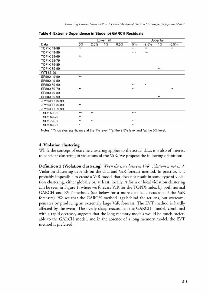
Table 3 shows the results from testing for dependence of residuals in normalGARCH residuals, and Table 4 does the same for a Student-t GARCH model. Asexpected, there is much less dependence in residuals. However, for some of thedatasets, the GARCH models fail to eliminate dependence. Even worse, if theextreme dependence is not of the GARCH type, the residuals may exhibit spuriousextreme dependence.

31


φλλ

λtt

t

r

r=

>≤

>>0

10

,

if

if

Table 1 Summary Statistics

Data From To Obs. Mean S.D. Skew. Kurt. AC(1) TOPIX 08/01/49 07/30/99 14,179 0.032% 0.88% –0.44 19.30 0.16TOPIX 08/01/49 07/31/59 3,007 0.052% 0.90% –0.12 12.41 0.25TOPIX 08/01/59 07/31/69 3,006 0.021% 0.72% –0.36 6.46 0.16TOPIX 08/01/69 07/31/79 2,896 0.039% 0.69% –1.44 17.28 0.22TOPIX 08/01/79 07/31/89 2,803 0.063% 0.49% –2.41 70.62 0.10TOPIX 08/01/89 07/30/99 2,467 –0.023% 1.25% 0.30 7.81 0.11WTI 06/01/83 07/30/99 4,021 –0.010% 2.45% –1.38 28.87 0.01SP500 08/01/49 07/30/99 12,632 0.035% 0.85% –1.78 50.89 0.10SP500 08/01/49 07/31/59 2,518 0.055% 0.71% –0.83 10.27 0.10SP500 08/03/59 07/31/69 2,515 0.017% 0.63% –0.50 12.82 0.16SP500 08/01/69 07/31/79 2,543 0.005% 0.86% 0.29 5.45 0.24SP500 08/01/79 07/31/89 2,529 0.048% 1.09% –3.75 83.59 0.06SP500 08/01/89 07/30/99 2,527 0.053% 0.88% –0.50 9.31 0.01JPY/USD 08/01/79 07/30/99 5,093 –0.012% 0.71% –0.81 10.65 0.02JPY/USD 08/01/79 07/31/89 2,489 –0.018% 0.66% –0.39 5.48 0.04JPY/USD 08/01/89 07/30/99 2,604 –0.007% 0.76% –1.06 13.20 0.00TSE2 08/01/69 07/30/99 8,166 0.031% 0.70% –0.79 13.10 0.43TSE2 08/01/69 07/31/79 2,896 0.049% 0.63% –1.02 13.96 0.47TSE2 08/01/79 07/31/89 2,803 0.051% 0.54% –1.76 30.21 0.32TSE2 08/01/89 07/30/99 2,467 –0.012% 0.91% –0.31 7.29 0.45


Table 2 Extreme Dependence in Returns

Lower tail Upper tailData 5% 2.5% 1% 0.5% 5% 2.5% 1% 0.5%TOPIX 49-99 *** *** *** *** *** *** *** ***TOPIX 49-59 *** *** *** *** *** *** ***TOPIX 59-69 *** *** *** *** ***TOPIX 69-79 *** *** *** *** ***TOPIX 79-89 *** *** *** *** *** *** ** ***TOPIX 89-99 *** *** *** *** **WTI 83-99 *** *** *** *** *** *** *** ***SP500 49-99 *** *** *** *** *** *** *** ***SP500 49-59 **SP500 59-69 *** *** *** *** ** **SP500 69-79 *** *** *** *** *** *** *** ***SP500 79-89 *** *** *** *** *** *** ***SP500 89-99 *** *** *** *** ***JPY/USD 79-99 *** *** *** *** ***JPY/USD 79-89 *** *** *** *** *** *** ** ***JPY/USD 89-99 *** *** *** *** **TSE2 69-99 *** *** *** *** *** *** *** ***TSE2 69-79 *** *** *** *** *** *** *** ***TSE2 79-89 **TSE2 89-99 *** *** *** *** ** **

Notes: ***indicates significance at the 1% level, **at the 2.5% level and *at the 5% level.

Table 3 Extreme Dependence in Normal GARCH Residuals

Lower tail Upper tailData 5% 2.5% 1% 0.5% 5% 2.5% 1% 0.5%TOPIX 49-99 ** ** **TOPIX 49-59 *** **TOPIX 59-69 ***TOPIX 69-79TOPIX 79-89TOPIX 89-99 **WTI 83-99SP500 49-99 ***SP500 49-59SP500 59-69 * *SP500 69-79 ** ** **SP500 79-89 *** **SP500 89-99 ***JPY/USD 79-99JPY/USD 79-89JPY/USD 89-99 **TSE2 69-99TSE2 69-79 ***TSE2 79-89TSE2 89-99 * *


33


Table 4 Extreme Dependence in Student-t GARCH Residuals

Lower tail Upper tailData 5% 2.5% 1% 0.5% 5% 2.5% 1% 0.5%TOPIX 49-99 ** ** ** **TOPIX 49-59 *** ***TOPIX 59-69 ***TOPIX 69-79TOPIX 79-89TOPIX 89-99 **WTI 83-99SP500 49-99 ***SP500 49-59SP500 59-69 ** *SP500 69-79 ** ** **SP500 79-89SP500 89-99 **JPY/USD 79-99JPY/USD 79-89 **JPY/USD 89-99TSE2 69-99 *** ** ***TSE2 69-79 **TSE2 79-89 ** ** **TSE2 89-99 * **


4. Violation clusteringWhile the concept of extreme clustering applies to the actual data, it is also of interestto consider clustering in violations of the VaR. We propose the following definition:

Definition 2 (Violation clustering) When the time between VaR violations is not i.i.d.Violation clustering depends on the data and VaR forecast method. In practice, it isprobably impossible to create a VaR model that does not result in some type of viola-tion clustering, either globally or, at least, locally. A form of local violation clusteringcan be seen in Figure 1, where we forecast VaR for the TOPIX index by both normalGARCH and EVT methods (see below for a more detailed discussion of the VaRforecasts). We see that the GARCH method lags behind the returns, but overcom-pensates by producing an extremely large VaR forecast. The EVT method is hardlyaffected by the event. The overly sharp reaction in the GARCH model, combinedwith a rapid decrease, suggests that the long memory models would be much prefer-able to the GARCH model, and in the absence of a long memory model, the EVTmethod is preferred.

5. AsymmetryOne feature of conditional volatility models, such as the GARCH model, is theimplicit assumption of symmetry of the return distribution. As discussed below, thisis not correct. Usually, one of the tails is fatter than the other. For example, for equi-ties, the lower tail is commonly thicker than the upper tail. In general, if the markettrend is upwards, the upper tail is thinner than the lower tail, i.e. the market movesin small steps in the direction of the trend, and in large jumps away from the trend.In the 1990s, most major stock indices have a relatively thicker lower tail, except theNIKKEI. Since the GARCH model, and its immediate extended forms, are symmet-ric, due to conditional normality or Student-t distributional assumptions, they tendto underpredict losses relative to gains, and hence, for an unsuspecting risk manager,will provide false comfort. While, in theory, it is straightforward to extend theGARCH model to take into account asymmetry, this necessarily complicates themodel.

The EGARCH model by Nelson (1991) is sometimes used for volatility forecast-ing.


Figure 1 Risk Overshooting in TOPIX VaR Forecast

y h z z N

h L L z z E z ,

t t t t

t ii

i

q

ii

i

p

t t t

=

= +

−

+ −[ ]{ }= =

−

− − −∑ ∑

, ( , )

log ( )

~ 0 1

1 11 1

1

1 1 1ω α β θ γ

Returns

EVT VaR forecast

Normal GARCH VaR forecast

10 20 30 40 50 60 70 80 90 100-0.25

-0.2

-0.15

-0.1

-0.05

0.05

0.1

where θ and γ are the parameters of asymmetry, and Li is the lag operator. Theadvantage of this model is, primarily, its relation to stochastic volatility models.Hence, it provides a link to continuous time finance. For risk applications, the pri-mary advantage is the explicit asymmetry, where risk forecasts depend on the direc-tion of lagged marked movements. However, typically, when this model is estimated,the asymmetry parameters are non-significant, suggesting that this model is misspeci-fied. As a result, in risk applications, this model does not have any special advantageover the GARCH model, and since it is more complex than the GARCH, it cannotbe recommended for risk forecasting.

The best way to forecast risk would be to use skewed conditional distributions.This, however, is not commonly done, due to the difficulty of finding an appropriateskewed distribution and estimating its parameters.6. VaR volatilityOne feature of conditional volatility models, such as the GARCH, is that the volatil-ity of risk forecasts is very high. Table 5 shows some sample statistics of predictedVaR numbers for the first two quarters of 1999 for the TOPIX index. We see that, ina portfolio of ¥1 billion, a normal GARCH model predicts VaR ranging from ¥18million to ¥41 million. Since market risk capital is 3 × VaR, this would imply verylarge fluctuations in capital. If financial institutions actually set capital at this level, itwould imply very high financing costs, and most likely result in the institution keep-ing a higher capital level than necessary. The reason why this is largely irrelevant,from a regulatory point of view, is that the regulatory VaR is typically of an order ofmagnitude higher than required. One area where this problem is not academic is ininternal risk management, where VaR may be used, e.g. to set limits for traders. Sincefrequently fluctuating VaR limits would result in high variability in the size of posi-tions, this would be considered unacceptable in most cases. As a result, in practice,most banks would use various techniques to dampen VaR volatility. In many cases,the covariance matrix is updated at infrequent intervals, e.g. once every three months.This, of course, usually results in large jumps in the limits (which are derived fromthe covariance matrix) four times a year, which in itself creates problems.Alternatively, a dampening function on the covariance matrix could be used, e.g. amoving average. A better way would be to use a long memory model for volatility. Inthis case, the variance is neither stationary nor non-stationary, implying a fractaldimension. The advantage is that these models provide persistence in shocks that fallsbetween the extremely short horizon of the GARCH-type model and the infinite per-sistence of I (1) models, like RiskMetrics. Long memory models are, however, notori-ously difficult to work with, and have some way to go until they can be employed inregular risk management. Another common method is to dispense with conditionalvolatility-based methods altogether for the setting of limits, and perhaps use histori-cal simulation or extreme value theory. See Daníelsson (2000b) for more discussionon risk volatility.

35


III. Extreme Value Theory

In common statistical methods, such as GARCH, all observations are used in theestimation of a forecast model for risk, even if only one in 100 events is of interest.This, obviously, is not an efficient way to forecast risk. The basic idea behind extremevalue theory (EVT) is that, in applications where one only cares about large move-ments in some random variable, it may not be optimal to model the entire distribu-tion of the event with all available data. Instead, it may be better only to model thetails with tail events. For example, an engineer designing a dam is only concernedwith the dam being high enough for the highest waters. Regular days when thewaters are average simply do not matter. Extreme value theory is a theory of thebehavior of large, or extreme, movements in a random variable, where extreme obser-vations are used to model the tails of a random variable (see Figure 2). EVT has beenwidely used in diverse fields, such as engineering, physics, chemistry, and insurance.However, it is only recently that it has been applied to financial risk modelling.


Table 5 VaR Volatility in the TOPIX Index (Percentage Returns)

Name From To Mean S.E. Min. Max. ViolationsGARCH normal 1954/07/29 1999/07/30 –1.71 1.04 –28.28 –0.59 1.65%GARCH-t 1954/07/29 1999/07/30 –1.86 1.09 –22.30 –0.65 1.25%EVT 1954/07/29 1999/07/30 –2.20 0.70 –3.94 –1.03 1.17%GARCH normal 1996/01/04 1999/07/30 –2.64 0.91 –7.56 –1.43 1.48%GARCH-t 1996/01/04 1999/07/30 –2.90 0.92 –7.13 –1.75 0.91%EVT 1996/01/04 1999/07/30 –3.25 0.21 –3.94 –2.90 0.91%Returns 1999/01/04 1999/03/31 0.26 1.18 –2.41 3.70GARCH normal 1999/01/04 1999/03/31 –2.59 0.64 –4.12 –1.80GARCH-t 1999/01/04 1999/03/31 –2.79 0.61 –4.21 –2.04EVT 1999/01/04 1999/03/31 –3.18 0.03 –3.31 –3.09Returns 1999/04/01 1999/06/30 0.18 1.00 –2.01 3.24GARCH normal 1999/04/01 1999/06/30 –2.57 0.37 –3.57 –2.02GARCH-t 1999/04/01 1999/06/30 –2.82 0.40 –3.84 –2.23EVT 1999/04/01 1999/06/30 –3.17 0.03 –3.19 –3.09

Note: These are summary statistics of VaR predictions.

Figure 2 The Tail

(a) Entire distribution (b) Left tail

A. Theoretical BackgroundClassification of tails of distribution is often arbitrary. For example, a high kurtosis is,perhaps, the most frequently used indication of fat tails. This, however, is an incor-rect use of kurtosis, which measures the overall shape of the distribution. One way todemonstrate this is by Monte Carlo experiments. We generated repeated samples ofsize 2000 from a known fat-tailed distribution, the Student-t (3). For each sample,we excluded the largest and smallest 40 values. Our random sample was, hence, trun-cated from above and below, and clearly thin-tailed. However, the average excess kur-tosis was 7.1, falsely indicating fat tails. In addition, various models are frequentlylabeled as fat-tailed, e.g. the conditionally normal stochastic volatility (SV) model. Itcan be shown that, according to the criteria below, the SV model is thin-tailed. Note,in contrast, that the GARCH model is fat-tailed, since the return process feeds backto the volatility process.

Formally, random variables fall into one of three tails shapes, fat, normal, andthin, depending on the various properties of the distribution.

1. The tails are thin, i.e. the tails are truncated. An example of this is mortality.2. The tails are normal. In this case, the tails have an exponential shape. The

most common member is the normal distribution.3. The tails are fat. The tails follow a power law.

It is a stylized fact that financial returns are fat. Hence, we only need to consider thethird case. An extremely important result in EVT is that the upper tail1 of any fat-tailed random variable (x) has the following property:

(7)

where α is known as the tail index, and F (.) is the asymptotic distribution function.The reason why this is important is that, regardless of the underlying distribution ofx, the tails have the same general shape, where only one parameter is relevant, i.e. α.If the data are generated by a heavy-tailed distribution, then the distribution has, to afirst order approximation, a Pareto-type tail:

(8)

as Daníelsson and de Vries (1997b) and Daníelsson and de Vries (1997a)demonstrate that the distribution of the lower tail is

(9)

x → ∞.

37


1. This applies trivially to the lower tails as well.

lim( )( )

, , ,t

F txF t

x x→∞

−−−

= > >11

0 0α α

P X x ax a>{ } ≈ > >−α α, , , 0 0

F xmn

xX m

( ) ,≅

+

−

1

α

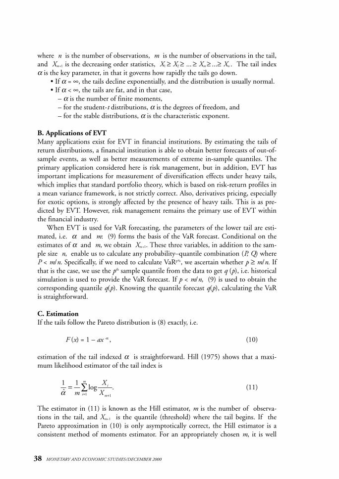
where n is the number of observations, m is the number of observations in the tail,and Xm+1 is the decreasing order statistics, X1 ≥ X2 ≥ ... ≥ Xm ≥ ...≥ Xn . The tail indexα is the key parameter, in that it governs how rapidly the tails go down.

• If α = ∞, the tails decline exponentially, and the distribution is usually normal.• If α < ∞, the tails are fat, and in that case,

– α is the number of finite moments,– for the student-t distributions, α is the degrees of freedom, and– for the stable distributions, α is the characteristic exponent.

B. Applications of EVTMany applications exist for EVT in financial institutions. By estimating the tails ofreturn distributions, a financial institution is able to obtain better forecasts of out-of-sample events, as well as better measurements of extreme in-sample quantiles. Theprimary application considered here is risk management, but in addition, EVT hasimportant implications for measurement of diversification effects under heavy tails,which implies that standard portfolio theory, which is based on risk-return profiles ina mean variance framework, is not strictly correct. Also, derivatives pricing, especiallyfor exotic options, is strongly affected by the presence of heavy tails. This is as pre-dicted by EVT. However, risk management remains the primary use of EVT withinthe financial industry.

When EVT is used for VaR forecasting, the parameters of the lower tail are esti-mated, i.e. α and m: (9) forms the basis of the VaR forecast. Conditional on theestimates of α and m, we obtain Xm+1. These three variables, in addition to the sam-ple size n, enable us to calculate any probability–quantile combination (P, Q) whereP < m/n. Specifically, if we need to calculate VaRp%, we ascertain whether p ≥ m/n. Ifthat is the case, we use the pth sample quantile from the data to get q (p), i.e. historicalsimulation is used to provide the VaR forecast. If p < m/n, (9) is used to obtain thecorresponding quantile q(p). Knowing the quantile forecast q(p), calculating the VaRis straightforward.

C. EstimationIf the tails follow the Pareto distribution is (8) exactly, i.e.

F (x) = 1 – ax -α , (10)

estimation of the tail indexed α is straightforward. Hill (1975) shows that a maxi-mum likelihood estimator of the tail index is

(11)

The estimator in (11) is known as the Hill estimator, m is the number of observa-tions in the tail, and Xm+1 is the quantile (threshold) where the tail begins. If thePareto approximation in (10) is only asymptotically correct, the Hill estimator is aconsistent method of moments estimator. For an appropriately chosen m, it is well


1 1

11ˆlog .

α=

+=∑

mX

Xi

mi

m

known that this estimator currently has the best empirical properties for the tailindex of financial returns. However, the choice of m is not trivial. Choosing m is thesame as determining where the tail begins. Choosing m arbitrarily, e.g. as 1 percent ofthe sample size, is not recommended. Hall (1990) proposes a subsample bootstrapmethod for the determination of m. His method relies on strong assumptions of thetail shape, and Daníelsson and de Vries (1997a) propose an automatic double sub-sample bootstrap procedure for determination of the optimal threshold, m*.1. The optimal thresholdThe choice of the optimal threshold m* is very important, since the estimates of αand, hence, risk, will vary highly by changing m. The optimal choice of m*.dependson the following results.

1. The inverse estimate of the tail index 1/ is asymptotically normally distrib-uted.

2. Therefore, we can construct the asymptotic mean square error(AMSE)of 1/ .3. Since, in general, 1/ is biased and is subject to estimation variance, we

need to take the following into account.

(a) As both the variance and bias are affected by the choice of m, it is opti-mal to choose m where the bias and variance vanish at the same rate.

(b) Therefore, the level where the AMSE is minimized gives us the optimalthreshold level, m*, i.e. we have

We obtain the AMSE by a bootstrap procedure. However, resampling of size Tdoes not eliminate variation in the AMSE, and a subsample bootstrap is needed. Hall(1990) proposes a subsample procedure, where he assumes an initial m level to obtainan initial α, as a proxy for 1/α in the AMSE, then obtains 1/ estimates for eachsubsample bootstrap realization, and chooses m*sub for the subsample where the aver-age is minimized. This is then scaled up to the full sample m* using α̂ sub and theassumption of where β is the parameter of the second order expansion ofthe limit law in (7). This however has two drawbacks:

1. a need to assume an initial α, and2. assumption of a value for the second order parameter β (Hall argues that β =

α is a good assumption, but for Student-t, β = 2).

Daníelsson and de Vries (1997a) propose an automatic procedure to determinem*, where they use a double subsample bootstrap to eliminate reliance on the initialα and assumption of . The difference statistic between the Hill estimator and theDaníelsson-de Vries estimator converges at the same rate and has a known theoreticalbenchmark which equals zero in the limit. The square of this difference statistic pro-

β̂

ˆ ˆβ αsub sub=

α̂

α̂α̂

α̂

39


m*ˆ

.= −

min AMSE

1α α

12

duces a viable estimate of the MSE[1/α] that can be minimized with respect to thechoice of threshold. Furthermore, in order to attain the desired convergence in prob-ability, instead of convergence of distribution that can be obtained, at most, by a fullsample bootstrap, they show that one needs to create resamples of a smaller size thanthe original sample with a subsample bootstrap technique. The reason is that twosamples with different sampling properties are needed for the estimation of the sec-ond order parameter β, which is used in scaling the subsample optimal threshold upto the full sample threshold, where the Hill estimator is used to obtain the full sam-ple α estimate.

D. Issues in Application of EVTWhile, sometimes, EVT is presented as a panacea for risk management, this is notcorrect. There are several issues which limit the applicability of EVT to the financialsector.1. Sample sizeWhile there is nothing intrinsic which limits the sample size in EVT applications, inpractice, there are constraints. There are primarily two types of constraints whichlimit the sample size from below.

1. We need to observe some events which constitute extremes, and2. most estimation methods for the threshold, m, depend on subsample boot-

strap or even double subsample bootstrap, which implies that the first con-straint has to be observed in all bootstrap subsamples.

If the Hill estimator is used for the determination of m, one requires, at the absoluteminimum, that the number of observations in the tail is m+1. However, m is esti-mated with a subsample procedure, where the size of the subsample should be assmall as is feasible. Practical experience and theoretical results indicate that the size ofthe subsample should be, perhaps, 10 percent of the sample size. Therefore, if thesample size is 1000, the subsample size is 100, and on average, one will observe 50positive values, from which to estimate the subsample values. However, in repeatedbootstraps, the particular bootstrap with the smallest number of positive observationswill provide the upper constraint on feasible positive values. In practice, this impliesthat 1,000 observations is the absolute minimum, and 1,500 observations is prefer-able. Having more than 6000 observations does not seem to make much of a differ-ence. The risk manager is, therefore, in a classical Catch22 situation; statisticaldemands may be inconsistent with the fact that the world is changing. Actually, thisis a reflection of a greater problem. In many markets, especially emerging markets,there is simply not enough data to do sensible analysis, whether by EVT or any othermethod. Perhaps for this reason, most published work on risk management is focusedon modelling risk in highly liquid, long running data series, such as SP-500.2. EVT is usually univariateWhile multidimensional EVT is actively being developed, it suffers from the samecurse of dimensionality problems as many other techniques, such as GARCH. As aresult, at the time of writing, such methods have very limited applicability in risk


management. There are, however, signs that this is changing, especially in the veryinteresting work of Longin (1999), where he measures how the covariance changes asone moves into the tails.3. DependenceEVT, as presented here, assumes that the data is i.i.d. This, however, is not a theoreticlimitation. Resnick ans (1996) have shown that the Hill estimator is consis-tent under certain types of dependence, such as GARCH.

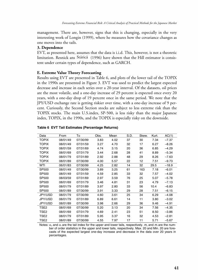
E. Extreme Value Theory ForecastingResults using EVT are presented in Table 6, and plots of the lower tail of the TOPIXin the 1990s are presented in Figure 3. EVT was used to predict the largest expecteddecrease and increase in each series over a 20-year interval. Of the datasets, oil pricesare the most volatile, and a one-day increase of 29 percent is expected once every 20years, with a one-day drop of 19 percent once in the same period. We note that theJPY/USD exchange rate is getting riskier over time, with a one-day increase of 9 per-cent. Curiously, the Second Section stocks are subject to less extreme risk than theTOPIX stocks. The main U.S.index, SP-500, is less risky than the major Japaneseindex, TOPIX, in the 1990s, and the TOPIX is especially risky on the downside.

Starica

41


Table 6 EVT Tail Estimates (Percentage Returns)

Data From To Obs. Mean S.D. Skew. Kurt. AC(1)TOPIX 08/01/49 07/30/99 3.83 4.02 37 30 7.34 –7.37TOPIX 08/01/49 07/31/59 3.27 4.70 32 17 6.27 –8.26TOPIX 08/01/59 07/31/69 4.74 3.15 20 36 6.85 –4.29TOPIX 08/01/69 07/31/79 3.44 2.68 28 41 8.89 –5.34TOPIX 08/01/79 07/31/89 2.92 2.88 48 29 8.26 –7.63TOPIX 08/01/89 07/30/99 4.00 5.57 22 12 7.51 –9.73WTI 06/01/83 07/30/99 4.25 2.82 14 32 29.5 –18.9SP500 08/01/49 07/30/99 3.89 3.25 61 163 7.18 –6.01SP500 08/01/49 07/31/59 4.59 2.85 33 32 7.57 –4.02SP500 08/03/59 07/31/69 2.97 3.59 76 25 5.07 –5.78SP500 08/01/69 07/31/79 3.46 4.81 31 23 4.79 –7.13SP500 08/01/79 07/31/89 3.97 2.80 33 56 10.4 –6.83SP500 08/01/89 07/30/99 3.91 3.33 29 28 7.51 –6.15JPY/USD 08/01/79 07/30/99 4.60 3.61 25 34 6.29 –4.08JPY/USD 08/01/79 07/31/89 6.89 6.61 14 11 3.80 –3.02JPY/USD 08/01/89 07/30/99 3.98 2.66 29 36 9.46 –4.91TSE2 08/01/69 07/30/99 5.20 3.13 20 34 7.56 –4.35TSE2 08/01/69 07/31/79 4.69 2.41 23 51 8.50 –3.86TSE2 08/01/79 07/31/89 5.95 3.37 16 32 4.53 –2.81TSE2 08/01/89 07/30/99 4.55 7.97 17 11 5.71 –5.67

Notes: αu and αl are the tail index for the upper and lower tails, respectively. mu and ml are the num-ber of order statistics in the upper and lower tails, respectively. Max. 20 and Min. 20 are fore-casts of the expected largest one-day increase and decrease in the data over 20 years inpercentages.


Figure 3 Lower Tails of the CDF for TOPIX 1990-1999

0.005

0.004

0.003

0.002

0.001

EmpiricalEstimated

Normal

8% 7% 6% 5% 4%

IV. Empirical Analysis

The empirical analysis is based on a variety of datasets from several periods. For mostparts, our empirical protocol was strictly non-data-snooping, i.e. we did not look atthe data before applying our procedures.

A. VaR PredictionsThe most common model for VaR forecasting is the GARCH class of models. Weuse the GARCH model with normal and Student-t innovations to forecast VaR. Theestimation window was 1000 observations, and the model is reestimated each day.We moved the 1000-day window to the end of the sample. Each day, we forecast thenext day’s VaR and count the number of violations. The results from this exercise,which are presented in Table 7, will not come as a surprise to readers of VaR litera-ture, since many authors have tested this and reached the same conclusions. The nor-mal GARCH model has the worst performance, followed by the Student-t GARCH,with EVT the best method. These results are especially interesting in light of theresults on VaR volatility below.

B. AsymmetryBoth the normal and Student-t GARCH models are based on the assumption of asymmetric conditional distribution, with no asymmetric responses of returns on therisk forecasts. As a result, these models assume that the unconditional distribution of

43


Table 7 VaR Violation Ratios

Lower tail Upper tail

Model Data 5% 2.5% 1% 0.5% 5% 2.5% 1% 0.5%

Normal TOPIX 4.50% 3.07% 1.98% 1.47% 4.10% 2.71% 1.59% 1.21%SP500 5.13% 3.40% 1.96% 1.41% 4.81% 2.93% 1.66% 1.19%JPY/USD 5.65% 3.84% 2.50% 1.89% 5.15% 3.23% 2.09% 1.53%WTI 5.08% 3.05% 1.98% 1.39% 4.80% 2.86% 1.90% 1.51%TSE2 4.76% 3.05% 2.04% 1.53% 5.06% 3.29% 1.86% 1.35%

GARCH TOPIX 5.14% 3.01% 1.65% 1.25% 4.05% 2.19% 1.05% 0.63%SP500 5.47% 3.33% 1.81% 1.12% 4.30% 2.31% 0.99% 0.59%JPY/USD 5.57% 3.42% 2.12% 1.64% 4.90% 2.84% 1.50% 1.00%WTI 5.04% 2.98% 1.71% 1.27% 4.40% 2.66% 1.43% 1.15%TSE2 5.25% 3.26% 1.82% 1.26% 4.34% 2.54% 1.22% 0.72%

GARCH-t TOPIX 5.80% 3.02% 1.25% 0.76% 4.44% 2.11% 0.71% 0.28%SP500 6.01% 3.18% 1.28% 0.60% 4.62% 2.11% 0.71% 0.34%JPY/USD 6.26% 3.01% 1.34% 0.92% 5.23% 2.31% 0.86% 0.19%WTI 6.27% 2.82% 1.15% 0.48% 4.68% 2.30% 0.99% 0.63%TSE2 5.39% 2.91% 1.29% 0.69% 4.76% 2.33% 0.89% 0.21%

EVT TOPIX 5.23% 2.68% 1.18% 0.69% 5.38% 2.90% 1.30% 0.72%SP500 5.61% 3.11% 1.27% 0.69% 5.55% 3.12% 1.27% 0.70%JPY/USD 5.51% 2.98% 1.31% 0.95% 6.43% 3.03% 1.53% 0.81%WTI 5.08% 2.94% 0.87% 0.48% 5.32% 2.78% 1.23% 0.63%TSE2 5.45% 2.72% 1.23% 0.72% 5.75% 2.99% 1.38% 0.78%

Notes: Length of Test: TOPIX=12,679, SP500=11,133, JPY/USD=3,593, WTI=2,521, TSE2=6,666.Each cell contains the ratio of VaR violations to total number of observations. The correctratio is in the top row.

returns is symmetric. This has two drawbacks for risk forecasting. First, it impliesthat the upper and lower tails are identical. However, this is clearly not the case. It iswell known that return distribution is not symmetric, with the upper tail typicallythinner than the lower tail. This is also the case with our data (see Table 6). In addi-tion, with the normal GARCH model, the thinner tail will be more important in theestimation, due to the exponential kernel. Hence, the thicker tail, typically the lower,will have a relatively lower impact on the estimation. We see that VaR predictionswith the GARCH model bear this out. There is considerable asymmetry in theGARCH results. The VaR levels in the upper tail are overpredicted, while those inthe lower tail are underpredicted.

C. VaR VolatilityAs discussed above, VaR volatility is of considerable concern. Table 5 shows statisticson VaR predictions for a portfolio of ¥1 billion of the various models under consider-ation. We first focus on the entire sample period. The normal GARCH model sug-gests that the largest one-day 1 percent VaR is ¥280 million, while the largest one-day loss on the TOPIX was only ¥150 million with an unconditional probability of0.007 percent, clearly indicating the implausibility of the GARCH results.Attempting to rectify the forecast by the use of a Student-t GARCH model does nothelp much, since its largest predicted loss is ¥220 million. A completely different pic-ture emerges from the EVT results. The VaR forecasts are stable, and do not have any


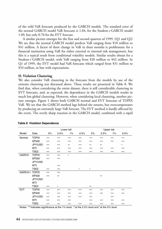
of the wild VaR forecasts produced by the GARCH models. The standard error ofthe normal GARCH model VaR forecasts is 1.04, for the Student-t GARCH model1.09, but only 0.70 for the EVT forecast.

A similar picture emerges for the first and second quarters of 1999. (Q1 and Q2)We see that the normal GARCH model predicts VaR ranging from ¥18 million to¥41 million. A factor of three change in VaR in three months is problematic for afinancial institution using VaR for either external or internal risk management, butthis is a typical result from conditional volatility models. Similar results obtain for aStudent-t GARCH model, with VaR ranging from ¥20 million to ¥42 million. InQ1 of 1999, the EVT model had VaR forecasts which ranged from ¥31 million to¥33 million, in line with expectations.

D. Violation ClusteringWe also consider VaR clustering in the forecasts from the models by use of theextreme clustering test discussed above. These results are presented in Table 8. Wefind that, when considering the entire dataset, there is still considerable clustering inEVT forecasts, and, as expected, the dependence in the GARCH models results inmuch less global clustering. However, when considering local clustering, another pic-ture emerges. Figure 1 shows both GARCH normal and EVT forecasts of TOPIXVaR. We see that the GARCH method lags behind the returns, but overcompensatesby producing an extremely large VaR forecast. The EVT method is hardly affected bythe event. The overly sharp reaction in the GARCH model, combined with a rapid

Table 8 Violation Dependence

Lower tail Upper tail

Model Data 5% 2.5% 1% 0.5% 5% 2.5% 1% 0.5%

Normal TOPIX *** *** *** *** *** *** *** ***SP500 *** *** *** *** *** *** *** ***JPY/USD *** *** ** *** ** ** *WTI *** *** *** *** *** *** *** ***TSE2 *** *** *** *** *** *** *** ***

GARCH TOPIX *** *** *SP500 *** ***JPY/USDWTI ***TSE2 *** *** * *

GARCH-t TOPIX *** ***SP500 *** ** **JPY/USDWTITSE2 *** * **

EVT TOPIX *** *** *** *** *** *** *** ***SP500 *** *** *** *** *** *** *** ***JPY/USD *** *** *** *** *** ***WTI *** *** *** *** *** *** ***TSE2 *** *** *** *** *** *** *** ***


45


decrease, suggests that the long memory models would be much preferable to theGARCH model, and in the absence of a long memory model, the EVT method ispreferred.

V. Conclusion

Risk management has undergone vast changes in recent years. Traditional methods,such as the GARCH class of models, have been pressed into service to provide riskforecasts, with mixed results. New techniques, such as extreme value theory (EVT),have been applied to the problem of risk forecasting. This is a dynamic field, and nosingle technical solution exists. One faces the classical problem of accuracy vs. com-plexity. In the paper, we compare and analyze the various methods for VaR forecast-ing of Japanese financial data.

We find that Japanese market data are well suited for advanced techniques, suchas EVT. The data exhibit patterns observed in other markets, rendering risk forecastsrelatively straight forward. By using EVT, we find that VaR forecasts are very accurateand stable over time. This implies that the use of EVT risk forecasting for Japanesefinancial institutions and other users of Japanese market data is recommended.

In contrast, we find that GARCH-type techniques are less accurate than EVTVaR forecasts, and even more worryingly, are very volatile. As a result, such modelscannot be recommended for practical VaR predictions. A detailed examination of theVaR forecasts from both EVT and GARCH models demonstrated that the wildswings observed in the GARCH VaR predictions are more an artifact of the GARCHmodel, rather than the underlying data. Finally, we note that a long memory modelwould provide the best risk forecasts. However, this cannot be recommended. This isbecause such models are notoriously difficult to estimate and require very long esti-mation horizons, effectively rendering them useless for most practical risk forecasting.

APPENDIX: EXTREME VALUE THEORY

This appendix gives an overview of the statistical methods that are used in obtainingthe estimated extreme tail distribution. The following is a brief summary of theresults in Daníelsson and de Vries (1997a), which also provides all the proofs; themethod has been applied by Daníelsson and de Vries (1997b).

Let x be the return on a risky financial asset where the distribution of x is heavy-tailed. Suppose the distribution function F(x) varies regularly at infinity with tailindex α:

(A.1)

This implies that the unconditional distribution of the returns is heavy-tailed andthat unconditional moments which are larger than α are unbounded. The assump-tion of regular variation at infinity, as specified in (A.1), is essentially the onlyassumption that is needed for analysis of the tail behavior of the returns x. Regularvariation at infinity is a necessary and sufficient condition for distribution of themaximum or minimum in the domain of attraction of the limit law (extreme valuedistribution) for heavy-tailed distributed random variables.

A parametric form for the tail shape of F(x) can be obtained by taking a secondorder expansion of F(x) as The only non-trivial possibility under mildassumptions is

(A.2)

The tail index can be estimated by the Hill estimator (Hill 1975), where m is the ran-dom number of exceedances over a high threshold observation Xm+1.

(A.3)

The asymptotic normality, variance, and bias are known for this estimator. It can beshown that a unique AMSE-minimizing threshold level exists, which is a function ofthe parameters and number of observations. This value can be estimated by the boot-strap estimator of Daníelsson and de Vries (1997a).

It is possible to use (A.2) and (A.3) to obtain estimators for out-of-sample quan-tile and probability (P, Q) combinations, given that the data exhibit fat-tailed distrib-uted innovations. The properties of the quantile and tail probability estimators belowfollow directly from the properties of . In addition, the out-of-sample (P, Q) esti-mates are related in the same fashion as the in-sample (P, Q) estimates.

To derive the out-of-sample (P, Q) estimator, consider two excess probabilities pand t with p < 1/n < t, where n is the sample size. Corresponding to p and t are thelarge quantiles, xp and xt , where for xi we have 1–F(xi) = i, i=t, p. Using the expansionof F (x) in (A.2) with β > 0, we can show that, by ignoring the higher order terms in

x → ∞.

lim( )( )

, , .t

F txF t

x x→∞

−−−

= > >11

0 0α α

F x ax bx o x x( ) , .= − + + ( )[ ] > → ∞− − −1 1 0α β β β as

1 1

11α=

+=∑

mX

Xi

mi

m

log


1/α̂

47


the expansion, and replacing t by m/n and xt by the (m+1)-th descending order statis-tic, one obtains the estimator

(A.4)

It can be shown that the quantile estimator is asymptotically normally distrib-uted. A reverse estimator can be developed as well by a similar manipulation of (A.2).

(A.5)

The excess probability estimator is also asymptotically normally distributed.p̂

x̂ p

ˆ .ˆ

x Xmnpp m=

+( )1

1α

ˆ .

ˆ

pmn

xx

t

p

=

α


Basel Committee on Banking Supervision, Overview of the Amendment to the Capital Accord toIncorporate Market Risk, 1996.

Bollerslev, T., “Generalised Autoregressive Conditional Heteroskedasticity,” J. Econometrics, 51, 1986,pp. 307–327.

Daníelsson, J., “Limits to Risk Modelling,” mimeo, London School of Economics, 2000a (www.risk.is).———, “(Un) Conditionality and Risk Forecasting,” mimeo, London School of Economics, 2000b

(www.risk.is).———, and C. G. de Vries, “Beyond the Sample: Extreme Quantile and Probability Estimation,”

mimeo, Tinbergen Institute Rotterdam, 1997a.———, and ———, “Tail Index and Quantile Estimation with Very High Frequency Data,” Journal

of Empirical Finance, 4, 1997b, pp. 241–257.Greenspan, A., “Discussion at Symposium: Maintaining Financial Stability in a Global Economy,” at

the Federal Reserve Bank of Kansas City, p. 54, 1997.Hall, P., “Using the Bootstrap to Estimate Mean Squared Error and Select Smoothing Parameter in

Nonparametric Problems,” Journal of Multivariate Analysis, 32, 1990, pp. 177–203.Hill, B. M., “A Simple General Approach to Inference about the Tail of a Distribution,” Annals of

Statistics, 1975, pp. 1163–1173.Longin, F., “From Value at Risk to Stress Testing: The Extreme Value Approach,” Discussion Paper

No. 2161, Center for Economic Policy Research, 1999.Morgan, J. P., Risk Metrics-Technical Manual, Third Edition, 1995.Nelson, D. B., “Conditional Heteroskedasticity in Asset Pricing: A New Approach,” Econometrica, 59,

1991, pp. 347–370.Resnick, S., and C. Sta% rica% , “Tail Index Estimation for dependent Data,” mimeo, School of ORIE,

Cornell University, 1996.

References

forecasting extreme financial risk: a critical … extreme financial risk: a critical analysis of...

Documents