forecasting house prices using dynamic model …

A Work Project presented as part of the requirements for the Award of a Master Degree in

Finance from the NOVA – School of Business and Economics.

FORECASTING HOUSE PRICES USING DYNAMIC MODEL AVERAGING

DIOGO ANTÓNIO MONTEZ DE SOUSA

Student Number 3145

A Project carried out on the Master in Finance Program, under the supervision of:

Professor Paulo M. M. Rodrigues

January 3, 2018

1

ABSTRACT

This work project applies the Dynamic Model Averaging methodology to forecast

quarterly house price growth in Portugal, Spain, Italy, Ireland, the Euro Area and the United

States. This recent econometric technique uses the Kalman filter to recursively estimate

dynamic models and ultimately produces a forecast by averaging these models using a

prediction performance criterion. Results show the superior predictive ability of this

methodology when compared to the usual autoregressive benchmarks. Furthermore, we make

use of the model’s outputs to provide a comparative analysis of the six series, concluding that

there is no single predictor transversally important for all series.

Keywords: House prices, Dynamic Model Averaging, Kalman Filter, Forecasting

2

1. INTRODUCTION

The housing sector is an essential sector of the economy, primarily because it satisfies a

basic need of the human being – shelter. In addition, the way most of our modern economies

are built, put houses as one of the major assets in which people tend to invest their money.

However, the role of the housing sector is larger and more complex than this. For instance,

housing feeds mortgage markets, which are important drivers in the transmission of monetary

policy and it is also argued that proper housing may facilitate labor mobility in the economy,

helping it to adjust to adverse shocks. Furthermore, house prices have a significant positive

impact on private consumption, residential investment and provide a useful indicator of demand

pressures in the economy. Bottom line, “as economies develop one should expect a deepening

and growth of housing markets” (Min Zhu speech at the IMF Conference, 2014).

The 2007/2008 recession urged the need to pay closer attention to this sector, which had

until then been somewhat neglected by macroeconomists in general. Widely read textbooks in

the field at the time, did not give real estate the due importance, as noted by Leamer (2007).

Leamer explains that “Housing is the most important sector in our economic recessions, and

any attempt to control the business cycle needs to focus especially on residential investment.”

A substantial increase in house prices contributes to an over-heating of the economy, whereas

its opposite is usually associated with an economic slowdown. When the economy is growing,

rising demand for housing pushes residential investment and construction employment upward,

strengthening aggregate demand. On the other hand, contraction phases are characterized by

falling income and job uncertainty, decreasing housing demand, reducing prices and the overall

attractiveness of residential investment; see e.g. Risse and Kern (2016).

This sector has experienced several booms and busts over time and the close connection

between sharp house price declines and financial recessions is well documented. In their famous

book about financial crises, This Time Is Different, Reinhart and Rogoff (2007) call attention

3

to the historical link between housing bubble bursts and banking crisis, both in advanced and

emerging economies. The pattern that is highlighted by the authors and had already been

addressed by Bordo and Jeanne (2002) refers that “a boom in real housing prices in the run-up

to a crisis is followed by a marked decline in the year of the crisis and subsequent years.” This

statement shows, once again, the unquestionable importance of the housing market and the

repercussions that its dynamics can have on the economy.

Considering all these facts, we can conclude that accurate house price forecasting is of

great importance to extract valuable information on the business cycle and to help governments

and policymakers to better regulate the real estate market, influencing the real economy. This

paper intends to add to the existent literature of house price forecasting using Dynamic Model

Averaging (DMA) and it closely relates with the works developed by both Wei and Cao (2017)

and Risse and Kern (2016), as we aim to use DMA to forecast real house price growth in several

European countries, namely peripheral countries such as Portugal, Spain and Italy, but also

other economies strongly affected by the financial crisis of 2008 like Ireland and the US.

2. LITERATURE REVIEW

Predicting house prices is a problem addressed by a vast number of scholars, which have

already produced quite extensive research on the topic, using a substantial quantity of different

methods. DiPasquale and Wheaton (1994) were pioneers in the application of some

macroeconomic variables to forecast house prices in the US and found that this approach led to

improvements in the models’ forecasting accuracy. Later, Brown et al. (1997) used time-

varying coefficients (TVC) models to forecast UK’s quarterly house price changes from 1968

to 1992, allowing for the introduction of a dynamic component inherent to markets in general

that was being neglect until then. The methodology of these authors rivals with previous studies

that assume that the underlying data generating process behind house price growth is stable and

apply constant parameter techniques, which may not exactly match reality. The housing market

4

tends to be exposed to structural shocks, such as institutional changes or government policies,

thus coefficient stability is not present, and a methodology that incorporates this instability

should be more appropriate to use. They show that the TVC model, in fact, yields better

forecasting performance when compared to alternative constant parameter regressions, such as

vector autoregressive (VAR) models, error correction mechanisms (ECM) and autoregressive

models.

The historical boom and bust cyclical behavior of real estate markets drew researchers’

attention, arousing the question of the existence of some heterogeneous regimes. Crawford and

Fratantoni (2003), focusing on five US states from 1979 to 2001, tested regime-switching

models, which also incorporate some instability by allowing the model to adapt itself to

different states. The study aimed to forecast quarterly variations in house prices and the main

conclusions were that despite achieving a good in-sample performance, the regime-switching

model did not outperform the classical ARIMA in the out-of-sample evaluation. According to

Miles (2008), some researchers have found in subsequent years that Markov-switching models

are particularly “ill-suited for forecasting”. Nevertheless, he also concludes that nonlinear

models improve the forecasting performance in housing markets, particularly when these are

subject to great volatility.

Rapach and Strauss (2009) use an autoregressive distributed lag (ARDL) model,

considering 29-35 potential predictors including state and regional economic variables to

forecast real house price growth in the 20 largest US states, in terms of population, from 1975

to 2006. They found substantial differences in forecasting house price growth in interior and

coastal states. In interior states, there is evidence that combining models with different lag

structures leads to accuracy improvements. However, in coastal states, house prices exhibit

some disconnection in relation to economic variables, making forecasting an (even more)

difficult task. This shows that there is no “one-size-fits-all” approach concerning house price

5

forecasting, suggesting that each market and region may experience different dynamics, even

if they belong to the same country.

Kouwenberg and Zwinkels (2015) rely on a different approach, as they try to exploit the

short-term positive serial correlation and long-term mean reversion to fundamental values that

real estate returns exhibit. These authors developed an econometric model (VECM with smooth

transition between components) that dynamically weights these two stylized facts depending

on the model’s recent performance. Such balance implies an overweight of the positive serial

correlation component in boom times when possible bubbles are gaining dimension and more

weight to reversal to fundamental values during subsequent downturns. They found that the

difference in forecasting performance is significantly better when compared to the fundamental

mean reversion models and the random-walk benchmark, however it is not shown to outperform

the classical AR(1). This result suggests that the problem with these models might lie in the

correct estimation of the fundamental value of houses, which is not very consistent. The

fundamental value estimate resembles the Gordon Model to value a stock’s fundamental value

based on dividends. This approach is based on a central assumption stating that the fundamental

value is not conditional on any exogenous information, apart from rent and price data. Plus, it

also requires the estimate of a constant discount and growth rates; and the assumption of an

equilibrium relationship that implies that the long-run rate of capital gains is equal to the growth

rate of rents. However, the characteristics of the real estate market, especially the lack of

effective short-selling mechanisms, introduce some efficiency problems that can potentially

undermine these assumptions and make fundamental value’s estimation an onerous challenge.

With the revived interest in forecasting variables that have the power to undermine the

entire economic stability, brought by the 2007 global financial crisis, novel methods and

techniques have been applied to economic forecasting, particularly from the machine learning

field. Jirong et al. (2011) presented a hybrid genetic algorithm and support vector machine (G-

6

SVM) approach to forecast the average selling house price in China, between 1993 and 2002.

Their results are ambiguous since they only compare them with another genetic algorithm and

do not provide a commonly used benchmark. Nonetheless, the support vector regressions

(SVR) methodology is gaining some popularity among researchers and Plakandaras et al.

(2014) propose a methodology that combines signal processing field tools with SVR. The

results are quite interesting, as they found that the forecasting ability of their model outperforms

the classical random walk, the Bayesian autoregressive and the Bayesian vector autoregressive

models, both in and out-of-sample. Moreover, they also show that the model can be used as a

warning system for sudden price drops, for instance, predicting the 2006-2009 US housing

market decline, up to 2 years ahead.

Ghysels et al. (2013) make a thorough classification of the recent literature on house price

forecasting, highlighting several problems with the more traditional models that motivate the

use of dynamic models. First, it was found that the effects of the determinants of house prices

change over time. As mentioned above, the relationships between fundamentals and house

prices are subject to structural breaks and it may also be the case that the effect that certain

variables have on the housing sector depend on time and market conditions. Second, research

also points out that a model with a specific set of variables may not perform consistently over

time, thus motivating the use of a model selection procedure that selects the best model at each

point in time (Koop and Korobilis, 2012). The idea is that movements in house prices may be

driven by different factors at different points in time, i.e. the best house price predictors during

house price booms are different in boom and bust periods (Bork and Møller, 2015). The issue

with the model selection procedure is that it comes with a huge computational task attached. To

illustrate the point, take the following example: with n predictors, one would need to evaluate

2𝑛 models at each point in time, which totalizes 2𝑛𝑇 models for a sample with T periods. With

sufficiently large n and T, it becomes computationally demanding and unfeasible. The model

7

averaging solution seems now compelling if one considers different sets of predictors as

separate models and compute the weighted average of all possible combinations of predictors.

The challenge here is that the weights used to combine the different models cannot be

constant over time, otherwise it will not be possible to have enough flexibility as to capture the

time-varying contribution of each model. The classical Bayesian model averaging (BMA) fails

at this point, as the weights assigned to each model over time are not time-varying (Próchniak

and Witkowski, 2013; Man, 2015). Focusing on this issue, researchers developed several

forecasting combination methods, namely the information-theoretic model averaging (ITMA)

proposed by Kapetanios et al. (2008). The ITMA method takes the Akaike information criterion

(AIC) of each individual model computed with respect to previous observations and then

updates the model probability in the BMA. Their paper adopts this new averaging scheme to

forecast inflation in the UK, concluding that it can be a powerful alternative to BMA and factor

models.

Raftery et al. (2010) address some issues mentioned above with a new method named

Dynamic Model Averaging (DMA). The methodology exposed in the paper is not directly

related to economic forecasting, notwithstanding it has deserved the attention of some

researchers. These authors aimed to solve the problem of online prediction when it is uncertain

what is the best prediction model to use and was initially applied to the prediction of the output

strip thickness for a cold rolling mill, where the output is measured with a time delay. The

parallelism with economic forecasting is quite straightforward, as frequently there is a lot of

uncertainty involved regarding which model to use and in the parameter estimation. Koop and

Korobilis (2012) used this technique to forecast quarterly US inflation and found substantial

improvements over both simple benchmark regressions and TVC models. The advantage of

the DMA approach lies in the fact that it allows for the model to change and parameters to shift,

adding the necessary flexibility to adapt to an ever-changing macroeconomic framework.

8

Additionally, this method combines the different models dynamically, using forgetting factors,

which approximate the evolution of model parameters and model switching probabilities; see

e.g. Wei and Cao (2017).

Bork and Møller (2015) were the first to apply DMA and Dynamic Model Selection

(DMS) forecasting techniques to house prices. Their paper examined the house price forecast

ability across the 50 US states and concluded that the accuracy of these new models’ forecasts

substantially improves in comparison with the usual OLS regressions and AR(1) model. They

highlight that the states where the housing markets had been the most volatile, were the ones in

which the model changes and parameter shifts were needed the most.

The focus of most research mentioned until now has been the US, where a state-specific

approach is justified by the heterogeneity of house price dynamics between states. Though,

other scholars have recently published research on the European and Chinese housing markets.

Wei and Cao (2017) apply the DMA method to forecast the monthly growth rate of house prices

in 30 major Chinese cities between 2007 and 2015. Their paper adds to the existent literature

by using a model confidence set test (MCS) to statistically evaluate the forecasting efficiency

of different models and by introducing a new predictor – the Google search index. This index

was based on the popularity of the Google online search for the binomial “city name + house

price”. Their results proved once again the superior predictive power of these models and

showed that the Google search index, in the last years of their sample, exhibits a greater

importance than the macroeconomic or monetary indicators to predict house prices in China.

This result should be taken into consideration in further studies on the housing market, as

nowadays, people heavily use internet searches to make more informed purchasing decisions.

The challenge here is to ensure the proper selection and quality of the data used to extract

information about online searches related to the house-buying process.

9

Risse and Kern (2016) applied the same methodology (DMA) to the six largest countries

of the European Monetary Union. Various macroeconomic, monetary and demographic

fundamentals were used to forecast quarterly house-price growth for Belgium, France,

Germany, Italy, the Netherlands and Spain in the period between 1975 and 2015. Their findings

show that there is no predictor that is equally important in all countries, across all time periods.

For instance, in France and Germany, house-price growth appears to be driven by

macroeconomic fundamentals (such as e.g. unemployment and CPI), while the Belgian market

is more influenced by industrial production and the term spread. The Italian market was found

to be rather peculiar, as no set of predictors proved to have a significant effect. Interestingly,

the Dutch market showed no influence from macroeconomic predictors, but solely the term

spread and credit supply. Finally, the Spanish housing market displays a wider influence of

variables, ranging from credit supply and industrial production to GDP and labor force. This

dynamic averaging scheme allows us to obtain the evolution of each variables’ probability of

inclusion over time. This feature is quite useful in order to understand what are the drivers of

each housing market and to see what is the behavior that they exhibit across time-periods.

The remaining sections of this paper are organized as follows: the econometric

methodology is discussed in Section 3; the data is described in Section 4 followed by the

empirical results in Section 5 and conclusion in Section 6.

3. ECONOMETRIC METHODOLOGY

3.1. Dynamic Model Averaging and Dynamic Model Selection

To better understand the methodology applied in this work project it is useful to consider

the following: suppose that we have a set of 𝐾 models that are built with different subsets of 𝑥𝑡

as predictors, where 𝑥(𝑘) for 𝑘 = 1, 2, … , 𝐾, denotes the subset belonging to each model. Assume

that the relation between the dependent variable and these predictors, can be written as

𝑦𝑡 = 𝑥𝑡−1(𝑘)′

𝛽𝑡(𝑘)

+ 𝜀𝑡(𝑘)

, 𝛽𝑡(𝑘)

= 𝛽𝑡−1(𝑘)

+ 𝜂𝑡(𝑘)

, (1)

10

where, 𝑥𝑡−1(𝑘)′

⊆ 𝑥𝑡−1′ for 𝑘 = 1, 2, … , 𝐾, denotes a specific predictor set, 𝛽𝑡

(𝑘) is the vector of

parameters respective to each predictor set, 𝜀𝑡~𝑖. 𝑖. 𝑑. 𝑁 (0, 𝑉𝑡(𝑘)

) and 𝜂𝑡~𝑖. 𝑖. 𝑑. 𝑁 (0,𝑊𝑡(𝑘)

). Let

𝐿𝑡 ∈ {1, 2, … , 𝐾} identify the model that applies at time 𝑡, Β𝑡 = (𝛽𝑡(1)′

, … , 𝛽𝑡(𝑘)′

) ′ and 𝑌𝑡 =

{𝑦1, … , 𝑦𝑡}. To produce a time 𝑡 forecast using information conditional on 𝑡 − 1, DMA requires

the computation of Pr(𝐿𝑡 = 𝑘|𝑌𝑡−1), i.e. the conditional probability of selecting model 𝑘 as the

right one to forecast. Then, the final prediction is made by averaging forecasts across the

different models, weighted by the respective probabilities. DMS follows a similar principle, but

the final prediction is based on the model with the single highest probability, Pr(𝐿𝑡 = 𝑘|𝑌𝑡−1).

The dynamic word in the methodology’s name is merged with the model averaging

feature, explained above, by allowing for different models to hold at different points in time.

Such flexibility is important in macroeconomic modelling, as we can allow not only for the

predictors of house prices but also their marginal impact to change over time. However, one

should be careful, since the method still suffers from the usual risk of suggesting models which

include many parameters – overparameterization. Attached to this, comes a great computational

burden when forecasting with a large number of predictors. Note that the number of predictors

increases exponentially the number of different forecasting models to be averaged, 𝐾. With 𝑛

predictors in 𝑥𝑡−1, the total number of different forecasting models will be 𝐾 = 2𝑛, at each point

in time.

The application of the model described in (1) can only proceed if some specification for

how predictors can get in and out of the model is modelled, in other words, a criterion for how

transition between models would occur. An alternative would be to specify a transition matrix,

𝑃, with elements 𝑝𝑖𝑗 = Pr(𝐿𝑡 = 𝑖|𝐿𝑡 = 𝑗) for 𝑖, 𝑗 = 1,… , 𝐾, using what is known as Markov

switching processes. Once again, the computational effort arises as a barrier, since we add the

additional estimation of the probability transition matrix, 𝑃, of dimensions 𝐾 × 𝐾. Thus, the

number of predictors does not need to be that large for inference to be very imprecise due to

11

(3)

(4)

(5)

the number of parameters in 𝑃. Bayesian inference through this alternative does not seem very

attractive, motivating Raftery et al. (2010) to use an approximation that allows for the

application of standard state space methods such as the Kalman filter.

The structure in (1) relates to the switching linear Gaussian state space models, which

imply that the state vector, Β𝑡, is broken into independent blocks, each one representing a

different model. This independence means that the predictive density of Β𝑡 depends on 𝛽𝑡(𝑘)

,

but conditionally on 𝐿𝑡 = 𝑘. By assuming this, it is possible to follow the accurate

approximation of Raftery et al. (2010), where the Kalman filter is run 𝐾 times.

The approximation mentioned above involves two parameters, λ and α, which the authors

defined as forgetting factors, and which assume values slightly below 1. To properly understand

these factors and how the algorithm works, let us consider the model in (1) ignoring the part of

model uncertainty. With given values for 𝑉𝑡(𝑘)

and 𝑊𝑡(𝑘)

, one can apply standard filtering results

to recursively estimate or forecast. The Kalman filter’s starting point assumes that the set of

parameters on Β𝑡−1 conditional on 𝐿𝑡 = 𝑘 and with information until 𝑡 − 1, (𝑌𝑡−1), follows a

normal distribution with the following moments

Β𝑡−1|L𝑡−1 = 𝑘, 𝑌𝑡−1~𝑁(�̂�𝑡−1(𝑘)

, Σ𝑡−1|𝑡−1(𝑘)

).

It proceeds with parameter prediction for the subsequent period with information conditioned

on the previous period,

Β𝑡|L𝑡−1 = 𝑘, 𝑌𝑡−1~𝑁 (�̂�𝑡−1(𝑘) , Σ𝑡|𝑡−1

(𝑘) ),

where,

Σ𝑡|𝑡−1(𝑘) = Σ𝑡−1|𝑡−1

(𝑘) +𝑊𝑡(𝑘).

The first forgetting factor, λ, enters here. Raftery et al. (2010) simplify calculations by replacing

equation (4) with

Σ𝑡|𝑡−1(𝑘) = 𝜆−1Σ𝑡−1|𝑡−1

(𝑘) ,

(2)

12

(6.1) (6.2)

(7)

(6)

which is equivalent to 𝑊𝑡(𝑘)

= (𝜆−1 − 1)Σ𝑡−1|𝑡−1(𝑘)

, where 0 < 𝜆 ≤ 1. This forgetting factor implies

that data 𝑗 time periods old is assigned with 𝜆𝑗 weight in comparison with the last period and it

implies an effective window size of 1

1−𝜆. Moreover, as it is set for the factor to assume a value

slightly below one, coefficients in the model will experience a gradual evolution. Now, by

applying this simplification, we can avoid the estimation or simulation of 𝑊𝑡(𝑘)

. Then, the

estimation of the parameters is achieved by the following updating equation:

Β𝑡|L𝑡 = 𝑘, 𝑌𝑡~𝑁(�̂�𝑡(𝑘)

, Σ𝑡|𝑡(𝑘)

).

Equation (6) is the final stage of the Kalman filter. To properly detail the meaning of (6), the

equations to estimate the first (6.1) and second (6.2) moments of the represented distribution

are exhibited below.

�̂�𝑡|𝑡(𝑘)

= �̂�𝑡|𝑡−1(𝑘)

+𝐾𝑡𝑒𝑡 Σ𝑡|𝑡(𝑘) = Σ𝑡|𝑡−1

(𝑘) −𝐾𝑡𝑥𝑡−1(𝑘) Σ𝑡|𝑡−1

(𝑘)

with 𝐾𝑡 = Σ𝑡|𝑡−1(𝑘) 𝑥𝑡−1

(𝑘)′ (𝑉𝑡(𝑘) + 𝑥𝑡−1

(𝑘)′Σ𝑡|𝑡−1(𝑘) 𝑥𝑡−1

(𝑘) )−1

, which corresponds to the Kalman gain and 𝑒𝑡 =

(𝑦𝑡 − 𝑥𝑡−1(𝑘)′�̂�𝑡−1

(𝑘) ) to the one-step-ahead prediction error. The Kalman filter implements nothing

more than an “average” between the one-step-ahead prediction and the measured value,

weighted by the Kalman gain. The inference process is repeated recursively as we advance

through time, nonetheless to start the process �̂�0(𝑘)

and Σ0(𝑘)

must be specified. Recursive

forecasting is completed using the predictive distribution

𝑦𝑡|𝑌𝑡−1~𝑁(𝑥𝑡−1

(𝑘)′�̂�𝑡−1(𝑘) , 𝑉𝑡

(𝑘) + 𝑥𝑡−1(𝑘)′Σ𝑡|𝑡−1

(𝑘) 𝑥𝑡−1(𝑘) ).

It is important to reinforce the idea that the application of the previous results in (2), (3)

and (6) is conditional on L𝑡 = 𝑘, consequently, the prediction and updating equations only

provide information on 𝛽𝑡(𝑘)

and not on the full vector Β𝑡. Therefore, we need a prediction

method that is not conditional on a specific model 𝑘 (unconditional prediction). As we have

already discussed, the specification of a transition matrix and posterior use of MCMC algorithm

to estimate the unconditional predictions is not suitable in practical terms, given its

13

(9)

(10)

(11)

(12) (13)

(8)

computational burden and parameter proliferation. We turn to another approximation as

suggested by Raftery et al. (2010), adding an additional forgetting factor, α, with interpretation

similar to 𝜆. To solve the issue of being conditioned on a particular model, we would need to

estimate the following equation:

𝑝(Β𝑡−1|𝑌𝑡−1) = ∑ 𝑝 (𝛽𝑡

(𝑘)|L𝑡−1 = 𝑘, 𝑌𝑡−1) Pr(L𝑡−1 = 𝑘|𝑌𝑡−1)𝐾

𝑘=1 ,

where 𝑝 (𝛽𝑡(𝑘)|L𝑡−1 = 𝑘, 𝑌𝑡−1) is given by (2). What (8) means is that the conditional distribution

(predictive density) of all parameters derived from every possible combination of models,

𝑝(Β𝑡−1|𝑌𝑡−1), is given by an average of the distribution of the parameters of each specific

model, 𝑝 (𝛽𝑡(𝑘)|L𝑡−1 = 𝑘, 𝑌𝑡−1), weighted by the respective probability of each model,

Pr(L𝑡−1 = 𝑘|𝑌𝑡−1). All we have left to estimate is this last probability.

Let 𝜋𝑡|𝑠,𝑙 = Pr(L𝑡 = 𝑙|𝑌𝑠), implying that Pr(L𝑡−1 = 𝑘|𝑌𝑡−1) = 𝜋𝑡−1|𝑡−1,𝑘. If we used the

transition probability matrix, 𝑃, with elements 𝑝𝑘𝑙 (probability of “jumping” from model 𝑘 to

model 𝑙), the model prediction equation would be

𝜋𝑡|𝑡−1,𝑘 = ∑ 𝜋𝑡−1|𝑡−1,𝑙𝑝𝑘𝑙𝐾𝑙=1 .

Instead, with the approximation suggested by Raftery et al. (2010) we obtain

𝜋𝑡|𝑡−1,𝑘 =𝜋𝑡−1|𝑡−1,𝑘𝛼

∑ 𝜋𝑡−1|𝑡−1,𝑙𝛼𝐾

𝑙=1

where 0 < 𝛼 ≤ 1 is set to a value slightly below 1. Following a Kalman filter type approach,

the model updating equation is

𝜋𝑡|𝑡,𝑘 =𝜋𝑡−1|𝑡−1,𝑘𝛼 𝑝𝑘(𝑦𝑡|𝑌

𝑡−1)

∑ 𝜋𝑡−1|𝑡−1,𝑙𝛼𝐾

𝑙=1 𝑝𝑙(𝑦𝑡|𝑌𝑡−1)

,

where 𝑝𝑙(𝑦𝑡|𝑌𝑡−1) is the predictive density of model 𝑙, i.e., the density of a 𝑁 (𝑥𝑡−1

(𝑙)′ �̂�𝑡−1(𝑙) , 𝑉𝑡

(𝑙) +

𝑥𝑡−1(𝑙)′Σ𝑡|𝑡−1

(𝑙) 𝑥𝑡−1(𝑙) ) distribution evaluated at 𝑦𝑡.

Finally, the DMA and DMS one-step ahead recursive forecast, which dynamically incorporates

the 𝐾 models will be, respectively:

�̂�𝑡𝐷𝑀𝐴 = ∑ 𝜋𝑡|𝑡−1,𝑘

𝐾𝑘=1 𝑥𝑡−1

(𝑘)′�̂�𝑡−1(𝑘)

, and �̂�𝑡𝐷𝑀𝑆 = 𝑥𝑡−1

(𝑘∗)′�̂�𝑡−1(𝑘∗)

.

14

(14)

(15)

As mentioned above, the DMA forecast is a result of averaging all 𝐾 models according to their

historical performances, reflected in the probability 𝜋𝑡|𝑡−1,𝑘. The DMS forecast just considers

the model with the best historical performance, 𝑘∗, thus the one with the highest probability

𝜋(𝑡|𝑡−1,𝑘∗).

To correctly understand the interpretation of the forgetting factor, α, note that the weight

of model 𝑘 at time 𝑡 is

𝜋𝑡|𝑡−1,𝑘 ∝ [𝜋𝑡−1|𝑡−2,𝑘𝑝𝑘(𝑦𝑡−1|𝑦𝑡−2)]

𝛼= ∏ [𝑝𝑘(𝑦𝑡−𝑖|𝑦

𝑡−𝑖−1)]𝛼𝑖

𝑡−1𝑖=1 .

Thus, model 𝑘 is over weighted at time 𝑡 if its forecasting performance, measured by the

predictive density 𝑝𝑘(𝑦𝑡−𝑖|𝑦𝑡−𝑖−1), was good in the recent past. To control for “recent past”, we

rely on an exponential decay with rate 𝛼𝑖, for observations 𝑖 periods ago. For instance, if 𝛼 =

0.99, the forecast performance 5 years ago with quarterly data receives 82% (0.995×4 ≅ 82%)

as much weight as the forecasting performance last period. On the other hand, with 𝛼 = 0.95,

this percentage drops to 36%, i.e. the lower the value of 𝛼, the faster information is forgotten.

If 𝜆 = 𝛼 = 1, DMA is just the standard approach to BMA using conventional linear forecasting

models with no time variation in coefficients, thus it is interesting to include this case as a

competitive model of DMA in our empirical analysis.

To estimate the error variance 𝑉𝑡(𝑘)

the suggestion of Koop and Korobilis (2012) is

followed. They avoid the computational burden of using a stochastic volatility or ARCH

specification by applying an Exponentially Weighted Moving Average (EWMA) to estimate

𝑉𝑡(𝑘)

, i. e.,

�̂�𝑡(𝑘) = √(1 − 𝜅)∑ 𝜅𝑗−1𝑡

𝑗=1 (𝑦𝑗 − 𝑥𝑗(𝑘)′�̂�𝑗−1

(𝑘) )2.

The use of EWMA estimators is common in finance applications and 𝜅 the decay factor

is recommended to be set at 0.97 for monthly data and 0.94 for daily data. Just like these authors,

15

(17) (18)

in this paper, we use quarterly data and so the chosen 𝜅 is 0.98. To obtain the volatility forecasts

�̂�𝑡+1|𝑡(𝑘)

we recursively approximate and get

�̂�𝑡+1|𝑡(𝑘)

= 𝜅�̂�𝑡|𝑡−1(𝑘)

+ (1 − 𝜅) (𝑦𝑡 − 𝑥𝑡(𝑘)′

�̂�𝑡(𝑘)

)2.

3.2. Evaluation of forecasts

Forecast evaluation is a crucial procedure in forecasting exercises, ultimately trying to

answer the question: “Which is the best forecasting model?”. The question is then what

forecasting evaluation measures should be used. In this paper, two well-known loss functions

are used: MAFE (Mean Absolute Forecast Error) and MSFE (Mean Squared Forecast Error),

i.e.,

𝑀𝐴𝐹𝐸 = 𝑁−1∑ |𝑦𝑡 − �̂�𝑡|𝑁𝑡=1 , and 𝑀𝑆𝐹𝐸 = 𝑁−1∑ (𝑦𝑡 − �̂�𝑡)

2𝑁𝑡=1 ,

where 𝑦𝑡 is the actual value of the real house price growth, �̂�𝑡 is the respective forecast and 𝑁

is the number of forecasts. These criteria are quite similar, yet some differences are worth

noting. Due to the quadratic loss function it uses, MSFE, assigns a relatively large weight to

large errors, thus being more suitable when this kind of errors are particularly problematic. On

the other hand, MAFE has the advantage of providing a real interpretation of its value, as it

represents the average difference between the forecast and the actual value, something that

cannot be achieved using MSFE.

3.2.1. The Clark and West Test

MAFE and MSFE are good measures to have a sense of how the forecasting accuracy

compares between forecasts. However, if we are interested in knowing which alternative model

presents the best predictive ability, considering the statistical significance of the forecasting

losses between models, we must apply more advanced methods. We follow the method used by

Bork and Møller (2015) and Risse and Kern (2016) that opt for the test proposed by Clark and

West (2007). They reference a paper by Clark and McCracken (2001) that shows that the

commonly used Diebold and Mariano (1995) statistic has a nonstandard distribution when

(16)

16

(20)

testing for the equal accuracy of forecasts from nested models. As we are precisely working in

a framework with nested models, we should use a methodology that is robust to this problem

instead – the Clark and West test. The new statistic proposed is adjusted and it is approximately

normally distributed in the case of nested models. The test statistic is defined as

𝑓𝒋,𝒕 = (𝑦𝑡 − �̂�𝑀𝐸𝐴𝑁,𝑡)𝟐− [(𝑦𝑡 − �̂�𝑗,𝑡)

𝟐− (𝑦𝑀𝐸𝐴𝑁,𝑡 − �̂�𝑗,𝑡)

𝟐],

where �̂�𝑀𝐸𝐴𝑁,𝑡 represents the historical forecast of 𝑦𝑡 using the historical mean benchmark and

�̂�𝑗,𝑡 represents the forecast of model 𝑗 = 𝐴𝑅1, 𝐷𝑀𝐴, 𝐷𝑀𝑆, for the different forgetting factor

levels. The Clark and West test is completed by regressing 𝑓𝒋,𝒕 on a constant and then testing its

significance using the underlying heteroscedasticity and autocorrelation corrected t-statistic.

Rejection of the null hypothesis means that model 𝑗 significantly overperforms the benchmark

from a statistical stand point. We have statistical evidence to reject the null, at the 5% level, if

the t-statistic is greater than 1.645, which is the corresponding critical value. For simplicity, the

test hereby described uses the historical mean forecast as the benchmark against which we

compare other models. Nonetheless, in this paper, we considered the AR(1) and AR(2) as

benchmarks to conduct the Clark and West test, since it is straightforward that almost every

model would outperform the historical mean forecast and in this way, we would be less

demanding than what is required.

4. DATA

The data set used to conduct this analysis consists of quarterly observations of the real

house price growth rate for Portugal, Italy, Spain, Ireland, the Euro Area and the US. Data was

provided by Banco de Portugal, OECD, ECB and INE. The dependent variable is calculated as

follows:

𝑦𝑖,𝑡 = 100 × [ln(𝑟ℎ𝑝𝑖,𝑡) − ln(𝑟ℎ𝑝𝑖,𝑡−1)]

where, 𝑖 = 1,… , 6, stands for the country’s index. The objective is to build forecasting models

tailored to each of the countries, providing an analysis of European peripheral countries’

(19)

17

(Portugal, Spain and Italy) housing market, adding Ireland, the Euro Area and the US to

establish comparisons. Table 1 depicts the main descriptive statistics of the house price growth

rate for the 5 countries considered, plus the Euro Area.

Table 1. Descriptive statistics of the dependent variable for each country.

Note: ADF stands for augmented Dickey-Fuller unit root test. The significance levels for the null hypothesis’

rejection (unit root) are represented as follows: 10% ‘*’, 5% ‘**’ and 1% ‘***’

Four out of the six series used have data available since the 70’s providing more than 180

observations each. However, Portugal and the Euro Area have shorter series counting with 116

and 148 observations, respectively. Regarding the behavior of the series, we can observe

substantial disparities. Portugal figures as the country with the lowest quarterly average real

house price growth (0.0207%), contrasting with the rest of the time series, where the average is

at least 10 times above this. From this country set, only Portugal and Italy posted averages

below the Euro Area. Ireland stands at the top of the six with a quarterly average growth rate

of 0.6908%, followed by Spain and the United States. The largest quarterly drop occurred in

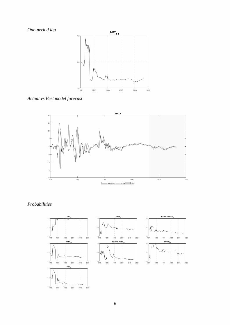
Italy in the first quarter of 1980, where real house prices fell almost 10%, largely due to a surge

in inflation at the time. Just a few years before, in 1973, the Italian real house prices increased

more than 15%, which represents the largest quarterly growth among all the series. These huge

ups and downs between the decade of 70 and 90 are a pattern that emerges in other countries as

well, namely in Ireland and Spain, where volatility spiked in this period as one can observe

from Figure 1. These three countries stand out with standard deviations at least two times above

the ones for Portugal, the Euro Area and the US, where movements went a lot smoother. A

quick look at the plots does not suggest a great correlation between the six series, though we

can see that from the end of 2007 until the end of 2013 real house prices fell, almost

Country Obs. Start End Mean Min. Max. Std. Dev. ADF

Portugal 116 1988.Q2 2017.Q1 0.0207 -3.7873 3.6691 1.4156 -5.4829***

Spain 184 1971.Q2 2017.Q1 0.5843 -5.9795 10.8534 2.7950 -5.4997***

Italy

188 1970.Q2 2017.Q1 0.2445 -9.8101 15.4302 3.3120 -6.1450***

Ireland 188 1970.Q2 2017.Q1 0.6908 -7.6876 11.0981 3.1086 -8.8122***

Euro Area 148 1980.Q2 2017.Q1 0.2739 -2.7273 2.1452 0.9353 -3.7228***

United States 188 1970.Q2 2017.Q1 0.3645 -3.8490 2.6937 1.1674 -5.7357***

18

uninterruptedly, in all of them and the cause of this tumble is well-known. After the burst of the

housing market bubble in the US in 2007/2008, the contagion effect spread the decline all over

Europe. The dimension of this drop is remarkable, though quite heterogeneous. In the period

between the end of 2007 and 2013, real house prices fell 63% in Ireland and 54% in Spain. Italy

and Portugal experienced a fall of around 20% and the Euro Area and the US 13% and 17%,

respectively. Additionally, Table 1 also shows the test statistic of the Augmented Dickey-Fuller

test for stationarity. The null hypothesis of the presence a unit root is rejected, at the 1%

significance level, for all series (as expected).

Figure 1. Quarterly real house price growth.

For fair forecast evaluation, each individual sample was divided into in and out-of-sample

data. Observations until and including the last quarter of 2006 were included in the training set,

using these data points to compute the priors to input at the start of the recursive estimation.

From the first quarter of 2007 onwards, the model does not include any forward-looking

information and is recursively estimated in each quarter.

The DMA methodology allows for the inclusion of a set of predictors for the dependent

variable, thus the model presented in this paper includes a group of 15 explanatory variables.

One can subdivide the set in 4 types of variables: macroeconomic (LABOR,

19

UNEMPLOYMENT, INCOME, GDP, GFCF and INFLATION), financial (SPREAD,

MORTGAGE), housing market specific (RENT, RENTPRICE, LOAN, CONSTCOST and

PERMITS) and lead sentiment indicators (CONSTCONF and CONFIDENCE). Table 2 lists

these regressors, briefly describing each of them and the transformations applied. The choice

of these variables was based on the variables used in previous research on this topic, including

also some new variables, namely RENTPRICE, MORTGAGE, GFCF, LOAN, CONSTCOST,

CONSTCONF and CONFIDENCE, with the objective to test if they are relevant predictors of

house prices.

Table 2. Description of the explanatory variables.

Transformation Codes: 1 – No transformation, 2 – First difference of natural logarithm

5. EMPIRICAL RESULTS

5.1. Average number of predictors

One of the remarkable advantages of the methodology used in this paper is its flexibility

concerning the number of different explanatory variables included in the model over time. The

inclusion or exclusion of each variable is conditioned on its recent past performance in terms

of predictive ability, measured by 𝜋. It would be interesting to see if the model does capture the

dynamic inclusion or exclusion of variables and how this number changes over time and across

# ID Tcode Description

1 LABOR 2 Total labor force in thousands

2 UNEMPLOYMENT 2 Unemployment rate

3 RENT 2 Rents index, calculated trough price-to-rent ratio

4 RENTPRICE 2 Rent to price ratio

5 SPREAD 2 10 years versus 3 months public debt spread

6 MORTGAGE 2 Real mortgage rate

7 INCOME 2 Real disposable income of households, in million euros

8 GDP 2 Real GDP, million euro or national currency (volume chained link

and market prices)

9 GFCF 2 Real GFCF (housing), real gross fixed capital formation, million

euros or national currency

10 LOAN 2 Loans to house purchase, base 2010

11 CONSTCOST 2 Construction costs index, base 2010

12 PERMITS 2 Number of housing permits, base 2010

13 CONSTCONF 2 Construction confidence index, base 2010 (Not available for Ireland)

14 CONFIDENCE 2 Economic sentiment indicator, base 2010 (Not available for Ireland)

15 PCD 2 Private consumption deflator, base 2010

20

countries. Koop and Korobilis (2012) show that the expected number of predictors, at time 𝑡,

will be

𝐸(𝑠𝑖𝑧𝑒𝑡) = ∑ 𝜋𝑡|𝑡−1,𝑘𝑠𝑖𝑧𝑒(𝑘)𝐾𝑘=1

where 𝑠𝑖𝑧𝑒(𝑘) is the number of explanatory variables in model 𝑘. Figure 2 contains the expected

number of coefficients in a historical time frame for the six series under analysis, for λ=α=0.95,

on the left and λ=α=1, on the right, for a DMA with the 15 variables in our dataset. These plots

show that the model size varies substantially across time. Additionally, it is possible to see a

positive relation between the factor values and the expected number of coefficients. For the

0.95 case, expected size ranges from 9 to 4, whereas for the other it also starts at 9, but quickly

decreases to values below 4. The conclusion is that the faster information is forgotten, the larger

we expect models to be, possibly because in this way the algorithm can adapt more easily and

allow for a larger number of predictors to input information on the final forecast.

Figure 2. Plot of the expected model size for DMA with (λ=α=0.95) and (λ=α=1)

5.2. Estimation process

To completely understand the results, it is important to know the process followed to

achieve them, therefore, the inclusion probabilities are of utmost relevance for a detailed and

correct perception of the empirical approach. Recall that in the DMA methodology these

probabilities are the weights used in the averaging of the different model forecasts, thus they

contain valuable information regarding the relative importance of each variable for the

movements in aggregate housing prices. Plots of these probabilities for (λ=α=0.95) are available

(21)

21

in the appendix. In addition to the variables included in Table 2, we also tested the model with

the inclusion of one lag of the dependent variable. The rationale for the inclusion of this lag is

that house price growth tends to exhibit a strong correlation with the previous period, mainly at

higher frequencies, like quarterly variations. Further evidence of this claim is reflected in the

probability plots with and without the lag that can be found in the appendix. A closer look at

these plots shows that in general, all probabilities decrease when the lag is included, which can

be interpreted as a caption of information by the lag itself. By looking at the probability plots,

some country independent conclusions can be taken. One of them is that sentiment variables

are rarely of great importance to predict house prices, being assigned with low (below 0.5)

probabilities of inclusion by the algorithm. The methodology itself can ignore less relevant

variables, by assigning them low probabilities of inclusion, nevertheless they still have a

considerable weight in the final forecast, especially if they produce extreme predictions, what

introduces a lot of “noise” in the system. With this issue in mind, we opted to exclude less

relevant variables (variables with historical inclusion probability below 0.5 during the training

period) from the set, building models as parsimonious as possible. Our findings reinforce the

idea of heterogeneity of the different housing markets and show that there is no single variable

that is an important predictor across the countries under analysis. Table 3 contains the models

with variables that have shown relevance during the training period, i.e. with probabilities above

0.5 within the training period, plus a one-period lag (LAG) of the dependent variable.

Table 3. Forecasting model’s composition.

In Portugal, we find the term spread, income and construction confidence as the regressors

with most importance in the training period. It is interesting to note that during the financial

Portugal Spain Italy Ireland Euro Area United States

LAG LAG LAG LAG LAG LAG

SPREAD UNEMPLOYMENT LABOR RENT MORTGAGE RENTPRICE

INCOME RENTPRICE UNEMPLOYMENT RENTPRICE GDP SPREAD

CONSTCONF INCOME RENT GDP GFCF GDP

- GDP RENTPRICE GFCF PCD LOAN

- - INCOME LOAN - PERMITS

- - PCD PCD - -

22

crisis specific variables instantly experienced increased probabilities, including variables that

were previously disregarded. This can be seen in the plots of INCOME (2008), GFCF (2008),

CONSTCOST (2008) and SPREAD (2011). The Spanish market displays different dynamics,

with a dominance of macroeconomic variables, such as the unemployment rate, income and

GDP, but also the rent-to-price ratio. The Italian house price growth series provides a clear

example of regime switching series. It is possible to conclude this by observing its plot in

Figure 1, where we can see a highly volatile behavior with huge variations, roughly until 1995,

and then volatility plummets, turning Italy into one of the most stable series of the sample. The

probability plots are consistent with this since several variables have plots peaking at the

beginning of the sample and then they abruptly decrease. This is the case for the unemployment

rate, rents, rent-to-price and the deflator, only labor force and income exhibit a slower decrease

of importance. In opposition to what we have seen above for Portugal, the financial turmoil

lived in 2007-2011 did not have a great impact on the probabilities for the Spanish and Italian

cases. The Irish housing market model is dominated by both housing market specific (RENT,

RENTPRICE, LOAN) and macroeconomic variables (GDP, GFCF and PCD). Rents and the

rent-to-price proved to have a great importance at the beginning of the sample that was rapidly

lost at the time and has been approximating past levels again, along with the loan to house

purchase series. Such as Portugal, the probability of inclusion of some variables spikes during

the 2007-2011 period, namely for rents, rent-to-price, the term spread and loan. Regarding the

Euro Area, the historical housing market growth rate displays very low volatility, mainly

because it is an average of a considerable number of different markets, thus softening its

behavior. The relevant variables in the in-sample period are all macroeconomic (GDP, GFCF

and PCD), except for the mortgage rate. The four variables produce quite similar plots, with

peaks at the beginning of the sample until mid-80’s and then a sudden drop, remaining low until

today. At present, these variables were surpassed in terms of probability of inclusion by the

23

loan to house purchase series. Finally, the US housing market shows some similarities with the

Euro Area, which makes sense as both are composed by smaller and heterogeneous housing

markets. As in the previous case, the most relevant variables (RENTPRICE, SPREAD, GDP,

LOAN and PERMITS), apart from GDP, have all very high probabilities of inclusion at the

start of the sample and then they all drop in a short time, becoming less significant. Analyzing

these probabilities as a whole, we could not disclose any pattern regarding the importance of

predictors among peripheral and non-peripheral countries. Even so, some variables seem to be

more relevant than others, for instance, the rent-to-price ratio appears to have substantial

importance in Portugal, Spain, Italy and the in US. Quite surprisingly, the unemployment rate

did not show a high probability of inclusion for any series, apart from Spain and, momentarily

the US in 2008. Although, its probability still presented a slight increase in 2008 for every

series, excluding Italy. Recently, we can observe that loan to house purchase describes a

growing importance in every country except in the US, where it stands stable at low levels.

As mentioned in Section 3.1, the values for λ and α set the degree of past information that

is considered at each point in time. Lower values for these factors mean a higher pace of

information forgetting, introducing more flexibility in the model. In this forecasting exercise, λ

and α were bound to the following set {0.95; 0.97; 0.99; 1}, which includes the optimal values

suggested by Koop and Korobilis (2012) for output and inflation forecasting. According to

these authors values below 0.95 may, sometimes, increase forecasting performance, though

they increase the possibility of overfitting. Therefore, we tested four DMA and four DMS, one

for each forecasting factor value. Additionally, to test our predictions, recursive AR(1) and

AR(2) models were estimated. A summary of the forecasting performance, for a quarterly

horizon, of the best models by country is depicted in Table 4 (please see Table 5 in the

Appendix for detailed results).

24

Table 4. Forecasting performance summary.

Note: The significance levels for the null hypothesis’ rejection are represented as follows: 10% ‘*’, 5% ‘**’ and 1% ‘***’

Overall, the results of this estimation are quite satisfactory, as all the best models beat the

MAFE and MSFE of the AR1 benchmark. The levels of improvement of the MSFE in relation

to the AR1 can be seen in the column ‘Relative MSFE’, where Portugal stands in last with

modest 0.82% and Ireland figures as the first with more than 80% improvement. When

comparing the MAFE and MSFE with the AR2 benchmark results are less positive, though

Italy, Ireland and US’s best models still outperform the two-lag autoregressive model.

Nonetheless, we are also interested in testing the differences in the forecasting performance of

different models, because MAFE and MSFE are mere averages. As mentioned in Section 3.2.1

we can do this using the Clark and West test (CW). This test was applied to test whether the

best model for each country was statistically better than the autoregressive benchmarks. Results

were promising as each of dynamic models proved to outperform both AR1 and AR2 in

forecasting house price growth, contradicting the MAFE and MSFE measures. The forecasting

loss function of MAFE and MSFE is not the same as the one used in the CW test, motivating

Forecasting method MAFE MSFE Rel. MSFE CW AR1 CW AR2

Portugal

AR1 1.1550 2.1690 1 - AR2 1.1304 2.0742 1.0457 -

DMA (λ=α=0.95) 1.0898 2.1514 1.0082 2.8523*** 2.7875***

Spain

AR1 1.1995 2.2989 1 - AR2 1.0668 1.8589 1.2367 -

DMA (λ=α=0.95) 1.0778 1.9136 1.2013 3.2059*** 2.7084***

Italy

AR1 0.5193 0.4699 1 - AR2 0.6614 0.7208 0.6520 -

DMS (λ=α=0.95) 0.4670 0.3719 1.2636 2.8990*** 4.0583***

Ireland

AR1 2.3736 8.8063 1 - AR2 2.1515 6.8913 1.2779 -

BMA (λ=α=1) 1.8324 4.7660 1.8477 4.2624*** 3.2692***

Euro Area

AR1 0.3894 0.2325 1 - AR2 0.3715 0.2086 1.1149 -

DMA (λ=α=0.99) 0.3871 0.2207 1.0534 2.0189*** 1.9343**

United States

AR1 0.7391 0.9763 1 - AR2 0.7453 0.9232 1.0576 -

DMS (λ=α=0.97) 0.6699 0.7069 1.3810 2.3621*** 2.7102***

25

the different conclusions. Nonetheless, being specifically designed to be applied to nested

models, the CW test is more reliable in this case.

6. CONCLUSION

This paper aimed to develop a comprehensive literature review of house price forecasting

and to apply a recent methodology to peripheral countries’ housing markets, as well as Ireland,

the Euro Area and the US. As the results show, the final objective of producing valid forecasting

models for this variable were met. However, some changes in the algorithm can potentially

improve our results, for instance, with the introduction of clusters instead of using the whole

span of forecasting models and with the use of dynamic processes to input optimal time-varying

forecasting factors.

A thorough review and explanation of the Dynamic Model Averaging algorithm were

made and the main advantages of it became clear, namely the way the econometrician can

include several predictors inside the system, so that the algorithm chooses the most important

ones at each point in time. This flexibility proved useful, not only to predict economic variables,

but also to analyze their behavior through the inclusion of probability plots. Our results

demonstrated the superior predictive ability of DMA and reinforced the idea that, despite the

increased globalization of economies and financial markets, each individual housing market is

subject to its own dynamic. The DMA methodology has already been applied to inflation and

house prices, nevertheless, the potential of DMA can go beyond these applications and be tested

with other macroeconomic variables, even outside of the economic scope. Possibly, pure

financial applications like multifactor stock pricing models are one area for further research

applying this method. Multifactor models can benefit from the model and parameter adaptation

of DMA, as classic approaches fail to incorporate the break of linear relationships or are too

slow to adapt to the new regimes.

26

7. REFERENCES

1. Bordo, M. D. and Jeanne, O. (2002). “Boom-Busts in Asset Prices, Economic

Instability, and Monetary Policy” National Bureau of Economic Research Working

Papers, No. 8966.

2. Bork, L. and Møller, S. (2015). “Forecasting house prices in the 50 states using Dynamic

Model Averaging and Dynamic Model Selection” International Journal of Forecasting,

31(1): 63-78.

3. Brown, J., Song, H. and McGillivray, A. (1997). “Forecasting UK house prices: A time

varying coefficient approach” Economic Modelling, 14(4): 529-548.

4. Clark, T. and McCracken, M. (2001). “Tests of equal forecast accuracy and

encompassing for nested models” Journal of Econometrics, 105(1): 85-110.

5. Clark, T. and West, K. (2007). “Approximately normal tests for equal predictive

accuracy in nested models” Journal of Econometrics, 138(1): 291-311.

6. Crawford, G. and Fratantoni, M. (2003). “Assessing the Forecasting Performance of

Regime-Switching, ARIMA and GARCH Models of House Prices” Real Estate

Economics, 31(2): 223-243.

7. Diebold, F. and Mariano, R. (1995). “Comparing Predictive Accuracy” Journal of

Business & Economic Statistics, 13(3): 253.

8. DiPasquale, D. and Wheaton, W. (1994). “Housing Market Dynamics and the Future of

Housing Prices” Journal of Urban Economics, 35(1): 1-27.

9. Ghysels, E., Plazzi, A. and Torous, W. (2013). “Forecasting Real Estate Prices”

Handbook of Economic Forecasting, 2: 509-580.

10. Girouard, N. and S. Blöndal (2001). “House Prices and Economic Activity” OECD

Economics Department Working Papers, No. 279, OECD Publishing, Paris.

11. Gu, J., Zhu, M. and Jiang, L. (2011). “Housing price forecasting based on genetic

algorithm and support vector machine” Expert Systems with Applications, 38(4): 3383-

3386.

12. Kapetanios, G., Labhard, V., Price, S. (2008). “Forecasting using Bayesian and

information theoretic model averaging: an application to UK inflation” Journal of

Business and Economic Statistics, 26: 33-41.

27

13. Koop, G. and Korobilis, D. (2012). “Forecasting Inflation Using Dynamic Model

Averaging” International Economic Review, 53(3): 867-886.

14. Kouwenberg, R. and Zwinkels, R. (2014). “Forecasting the US housing

market” International Journal of Forecasting, 30(3): 415-425.

15. Leamer, E. (2007). “Housing IS the business cycle”, Cambridge, MA: National Bureau

of Economic Research: 149-155.

16. Man, G., (2015). “Competition and the growth of nations: international evidence from

Bayesian model averaging” Economic Modelling, 51: 491–501.

17. Miles, W., (2008). “Boom-bust cycles and the forecasting performance of linear and

non-linear models of house prices” Journal of Real Estate Finance and Economics,

36(3): 249-264.

18. Plakandaras, V., Gupta, R., Gogas, P. and Papadimitriou, T., (2014). “Forecasting the

U.S. Real House Price Index” SSRN Electronic Journal.

19. Próchniak, M. and Witkowski, B., (2013). “Time stability of the beta convergence

among EU countries: Bayesian model averaging perspective” Economic Modelling, 30:

322-333.

20. Raftery, A., Kárný, M. and Ettler, P. (2010). “Online Prediction Under Model

Uncertainty via Dynamic Model Averaging: Application to a Cold Rolling

Mill” Technometrics, 52(1): 52-66.

21. Rapach, D. and Strauss, J. (2009). “Differences in housing price forecastability across

US states” International Journal of Forecasting, 25(2): 351-372.

22. Reinhart, C. and Rogoff, K. (2008). “This Time is Different”, Cambridge, Mass:

National Bureau of Economic Research.

23. Risse, M. and Kern, M. (2016). “Forecasting house-price growth in the Euro area with

dynamic model averaging” The North American Journal of Economics and Finance,

38: 70-85.

24. Wei, Y. and Cao, Y. (2017). “Forecasting house prices using dynamic model averaging

approach: Evidence from China” Economic Modelling, 61: 147-155.

25. Zhu, M. (2014). “Housing Markets, Financial Stability and the Economy” Opening

Remarks at the Bundesbank/German Research Foundation/IMF Conference.

Accessed September 21, 2017.

https://www.imf.org/en/News/Articles/2015/09/28/04/53/sp060514

https://www.imf.org/en/News/Articles/2015/09/28/04/53/sp060514

APPENDIX

1

Portugal

Probabilities

Probabilities with one lag

2

One-period lag

Actual vs Best model forecast

Probabilities

3

Spain

Probabilities

Probabilities


4

One-period lag


Probabilities

5

Italy

Probabilities


6

One-period lag


Probabilities

7

Ireland

Probabilities


8

One-period lag


Probabilities

9

Euro Area

Probabilities


10

One-period lag


Probabilities

11

United States

Probabilities


12

One-period lag


Probabilities

13

Table 4. Forecasting performance summary.



Portugal

AR1 1.1550 2.1690 1 - AR2 1.1304 2.0742 1.0457 -

DMA (λ=α=0.95) 1.0898 2.1514 1.0082 2.8523*** 2.7875***

Spain

AR1 1.1995 2.2989 1 - AR2 1.0668 1.8589 1.2367 -

DMA (λ=α=0.95) 1.0778 1.9136 1.2013 3.2059*** 2.7084***

Italy

AR1 0.5193 0.4699 1 - AR2 0.6614 0.7208 0.6520 -

DMS (λ=α=0.95) 0.4670 0.3719 1.2636 2.8990*** 4.0583***

Ireland

AR1 2.3736 8.8063 1 - AR2 2.1515 6.8913 1.2779 -

BMA (λ=α=1) 1.8324 4.7660 1.8477 4.2624*** 3.2692***

Euro Area

AR1 0.3894 0.2325 1 - AR2 0.3715 0.2086 1.1149 -

DMA (λ=α=0.99) 0.3871 0.2207 1.0534 2.0189*** 1.9343**

United States

AR1 0.7391 0.9763 1 - AR2 0.7453 0.9232 1.0576 -

DMS (λ=α=0.97) 0.6699 0.7069 1.3810 2.3621*** 2.7102***

14

Table 5.a Forecasting performance (all models).


Portugal

AR1 1.1550 2.1690 1 -

AR2 1.1304 2.0742 1.0457 -

DMA (λ=α=0.95) 1.0908 2.2319 0.9718 2.3074*** 2.1185***

DMA (λ=α=0.97) 1.0900 2.2083 0.9822 0.6698 0.0690

DMA (λ=α=0.99) 1.0997 2.2167 0.9785 0.5531 0.0053

BMA (λ=α=1) 1.1119 2.2287 0.9732 0.5367 0.1078

DMS (λ=α=0.95) 1.0714 2.2952 0.9450 2.1407*** 2.0407***

DMS (λ=α=0.97) 1.1214 2.3696 0.9153 0.3898 -0.1481

DMS (λ=α=0.99) 1.1702 2.4636 0.8804 0.0833 -0.4341

BMS (λ=α=1) 1.1354 2.3540 0.9214 0.4462 0.0448

Spain

AR1 1.1995 2.2989 1 -

AR2 1.0668 1.8589 1.2367 -

DMA (λ=α=0.95) 1.0345 1.7803 1.2913 3.7039*** 3.7108***

DMA (λ=α=0.97) 1.0346 1.7795 1.2919 3.6860*** 3.6974***

DMA (λ=α=0.99) 1.0213 1.7662 1.3016 3.6387*** 3.6308***

BMA (λ=α=1) 1.0290 1.7798 1.2916 3.5309*** 3.5240***

DMS (λ=α=0.95) 0.9965 1.7596 1.3065 3.6157*** 3.5451***

DMS (λ=α=0.97) 0.9991 1.7632 1.3038 3.6314*** 3.5517***

DMS (λ=α=0.99) 1.0282 1.7849 1.2880 3.4967*** 3.4952***

BMS (λ=α=1) 1.0282 1.7849 1.2880 3.5077*** 3.5066***

Italy

AR1 0.5193 0.4699 1 -

AR2 0.6614 0.7208 0.6520 -

DMA (λ=α=0.95) 0.4653 0.3776 1.2444 3.8966*** 5.3754***

DMA (λ=α=0.97) 0.4653 0.3775 1.2447 3.8941*** 5.3937***

DMA (λ=α=0.99) 0.4736 0.3884 1.2099 3.6015*** 5.4095***

BMA (λ=α=1) 0.4734 0.3919 1.1991 3.4379*** 5.3895***

DMS (λ=α=0.95) 0.4670 0.3719 1.2636 4.1849*** 5.5104***

DMS (λ=α=0.97) 0.4819 0.4025 1.1675 3.6140*** 5.5101***

DMS (λ=α=0.99) 0.4723 0.3907 1.2028 3.4384*** 5.3911***

BMS (λ=α=1) 0.4723 0.3907 1.2028 3.4384*** 5.3911***


15

Table 5.b Forecasting performance (all models).


Ireland

AR1 2.3736 8.8063 1 -

AR2 2.1515 6.8913 1.2779 -

DMA (λ=α=0.95) 1.8050 4.8469 1.8169 3.4653*** 3.3375***

DMA (λ=α=0.97) 1.8333 4.9638 1.7741 3.1409*** 2.6876***

DMA (λ=α=0.99) 1.9656 5.4493 1.6160 3.3439*** 2.4607***

BMA (λ=α=1) 1.9562 5.5372 1.5904 3.6414*** 2.6122***

DMS (λ=α=0.95) 2.0697 6.8086 1.2934 2.6624*** 2.5394***

DMS (λ=α=0.97) 2.1879 7.0763 1.2445 2.3038*** 1.9318**

DMS (λ=α=0.99) 2.2802 9.3070 0.9462 1.6979* 0.5653

BMS (λ=α=1) 1.9337 5.7863 1.5219 3.7146*** 2.8781***

Euro Area

AR1 0.3894 0.2325 1 -

AR2 0.3715 0.2086 1.1149 -

DMA (λ=α=0.95) 0.3569 0.1996 1.1652 2.5580*** 2.8758***

DMA (λ=α=0.97) 0.3589 0.1991 1.1679 2.5829*** 2.9004***

DMA (λ=α=0.99) 0.3575 0.1967 1.1822 2.6389*** 2.9405***

BMA (λ=α=1) 0.3561 0.1958 1.1874 2.6545*** 2.9504***

DMS (λ=α=0.95) 0.3544 0.1952 1.1913 2.6722*** 2.9729***

DMS (λ=α=0.97) 0.3559 0.1957 1.1880 2.6582*** 2.9541***

DMS (λ=α=0.99) 0.3559 0.1957 1.1880 2.6555*** 2.9506***

BMS (λ=α=1) 0.3559 0.1957 1.1880 2.6555*** 2.9506***

United States

AR1 0.7391 0.9763 1 -

AR2 0.7453 0.9232 1.0576 -

DMA (λ=α=0.95) 0.6830 0.7326 1.3327 3.4114*** 3.3298***

DMA (λ=α=0.97) 0.6795 0.7274 1.3422 2.2692*** 2.5480***

DMA (λ=α=0.99) 0.6818 0.7517 1.2988 2.2192*** 2.3037***

BMA (λ=α=1) 0.6975 0.8134 1.2003 1.9875*** 1.8453**

DMS (λ=α=0.95) 0.6739 0.7188 1.3582 3.4851*** 3.1733***

DMS (λ=α=0.97) 0.6699 0.7069 1.3810 2.3621*** 2.7102***

DMS (λ=α=0.99) 0.6896 0.7855 1.2429 2.1059*** 2.0668***

BMS (λ=α=1) 0.7110 0.8268 1.1809 2.0038*** 1.8091**


forecasting house prices using dynamic model …

Documents