forecasting limit order book price changes using change...

SCHOOL OF ECONOMICS

Forecasting

book price changes

change point detection

LUND UNIVERSITY

DEPARTMENT OF ECONOMICS

SCHOOL OF ECONOMICS AND MANAGEMENT

Forecasting limit order

price changes using


Master Thesis

Author: Sebastian Thorburn

Supervisor: Hossein Asgharian

Spring 2015

limit order

using


2

Title Forecasting limit order book price changes

using change point detection

Course NEKN01 Master Essay

Author Sebastian Thorburn

Supervisor Hossein Asgharian

Purpose The main purpose of this thesis is to propose

a method for using a change point detection

algorithm to forecast short term limit order

book price changes. The idea is to test

whether a significant change of the shape of

the limit order book contains any

information about impending price changes.

Method Using a data set consisting of all the changes

of the limit order book throughout the

trading day, a change point detection

algorithm is used to detect what is deemed to

be significant changes. A measurement of the

limit order imbalance is constructed as a

proxy for the shape of the order book which

then is used as input signal to the change

point detection algorithm. A new data set is

created based on the detected change points

and a regression is run based on these to

forecast impending price changes. To

benchmark the results, the original data set

is also sampled at a 5 minute interval and the

limit order imbalance measurement is

calculated for each observation. A regression

based on this data is then run to forecast

impending price changes. Regression results

from the two models are then compared.

Conclusions When forecasting impending price changes,

regressions based on the change point data

set yields better results than regressions

based on the 5 minute interval sample. It is

concluded that the data set created using

change point detection contains a certain

amount of information about impending

price changes.

Keywords Change point detection, high frequency

finance, limit order book, econometrics,

market microstructure

3

Contents List of figures .............................................................................................................................. 4

List of tables ............................................................................................................................... 4

1 Introduction ........................................................................................................................ 5

1.1 Background .................................................................................................................. 5

1.2 Problem discussion and purpose ................................................................................. 6

1.3 Focus and limitations ................................................................................................... 7

1.4 Outline of the thesis .................................................................................................... 8

2 Theoretical framework ....................................................................................................... 9

3 Method.............................................................................................................................. 12

3.1 The data set ............................................................................................................... 12

3.2 Model specification ................................................................................................... 13

3.2.1 Stock filtering...................................................................................................... 14

3.2.2 Constructing a limit order imbalance measure .................................................. 15

3.2.3 Specification of change point detection algorithm ............................................ 17

3.2.4 Specification of regression model ...................................................................... 23

4 Results ............................................................................................................................... 26

5 Analysis ............................................................................................................................. 31

6 Conclusion ......................................................................................................................... 33

6.1 Discussion of findings ................................................................................................ 33

6.2 Suggestions for further research ............................................................................... 34

7 References ........................................................................................................................ 36

7.1 Printed sources .......................................................................................................... 36

7.2 Electronic sources ...................................................................................................... 37

8 Appendix ........................................................................................................................... 38

8.1 Source code ............................................................................................................... 38

4

List of figures

Figure 1 Information flow during online change point detection............................................ 10

Figure 2 Matrix illustrating the four detection cases ............................................................... 10

Figure 3 Illustration of a data point of the limit order book, symbol SCV B ............................ 13

Figure 4 Limit order imbalance measure, ticker symbol TOP, first trading day of data set .... 17

Figure 5 Simulated input signal; constant mean, drift in mean, constant mean ..................... 19

Figure 6 First example of the CUSUM algorithm in action ....................................................... 20

Figure 7 Simulated data series, sudden shift in mean ............................................................. 20

Figure 8 CUSUM algorithm on simulated series, simulated mean .......................................... 21

Figure 9 Simulated data series, sine wave ............................................................................... 21

Figure 10 Third example of the CUSUM algorithm in action ................................................... 22

Figure 11 Example of a CUSUM series for detecting an upward change ................................. 23

Figure 12 Example of a CUSUM series for detecting an downward change ............................ 23

List of tables

Table 1 Regression results, change point sample .................................................................... 27

Table 2 Summary of regression results, change point sample ................................................ 28

Table 3 Regression results, 5 minute interval sample ............................................................. 29

Table 4 Summary of regression results, 5 minute interval sample .......................................... 30

Table 5 Regression summary, both data samples .................................................................... 31

5

1 Introduction

This chapter provides an introduction to the thesis with background, problem, purpose,

limitations and outline.

1.1 Background

Financial markets have existed for a very long time. An example of an old financial market is

that of tulip trading in the Netherlands, in which the infamous tulip bubble emerged in the

first half of the 17th century. Along with the actual markets, time series of financial trading

have also existed for a very long time. Historically, these have generally consisted of the last

traded price at regular time intervals such as monthly, weekly or daily close prices.

Depending on the particular usage of the times series at hand, the interval has varied. Before

computers revolutionized the financial markets, most of the trading volume occurred in

open out-cry pits where humans would gesticulate and scream their trading intentions. With

the advent of electronic marketplaces, when computers in the 1980s started becoming an

integral part of financial markets, the data started becoming more available and at a finer

resolution. Today trading almost exclusively occurs on electronic exchanges and as a result,

the amount of data that is stored and subsequently available for study is very big. Along with

technological advancements, the data not only becomes larger and larger in size, but also

more complex. Today, it is not only the last traded price at a regular time interval that is

available, but a plethora of information related to the matching process between buyers and

sellers and thereby the price discovery process (Fadiman, 2004).

Many aspects of the financial markets are of interest for scientific study. One of them is the

process of price discovery, but with the mentioned increased granularity of the data

available other methods than a simple linear regression of the last traded price are required.

In recent years that study and application of high frequency finance has emerged. Different

exchanges have different order types, different rules for the sequence in which orders are

matched against each other, different rules for the minimum allowed price increments of

the assets being traded, different opening hours, different rules for pre- and post-trade

anonymity, et cetera. These are all features of the market microstructure, which in turn is

much related to high frequency finance (Aldridge, 2010). It has been noted that market

microstructure features such as the minimum allowed price increment of an asset is an

integral part of short term price formation (Goldstein, 2000). At the core of all of this is the

6

essence of the actual facility for matching buyers and sellers; the limit order book. This is

where all the unmatched orders rest. The study of the limit order book is at the foundation

of this thesis.

1.2 Problem discussion and purpose

An arbitrary data set consisting of a million data points, where say 80% of them are pure

noise, can hide a lot of information from standard statistical techniques. Furthermore, if the

data points are complex in nature, perhaps in the form of an object rather than a scalar, this

also increases the difficulty in the analysis. Adding to this, if the data points are

heterogeneous in time, i.e. not evenly spread out with a constant time interval in between

them, this might add even more difficulty for the scientist about to study it.

Historically, initially just intraday data shed new light on the process of price discovery.

Today a completely new paradigm has been reached in the world of financial data where not

only the last transaction price is recorded, but also all available resting limit orders as well.

This obviously presents opportunities for the researcher about to study price discovery and

market microstructure in depth. However, how to handle such a data set is not as obvious as

how to handle a time series of say monthly close price. With a data sample of reasonable

size it’s fairly straight forward to run a regression. With the complete order book at the

market open and each and every consecutive update of it during the rest of the day, it is an

immense amount of data in comparison and not as straight forward how to approach it.

Another issue is that the limit order book is a collection of data at each observation. It is not

clear how the data should be represented in a model, as it no longer only consists of a

closing price but rather a range of values. Also, when and how the order book updates is

highly irregular and nonlinear (Cont, 2011). Furthermore, the sheer size of a high frequency

financial data set makes it hard to analyze. Many of the observations could be referred to as

noise (Aït-Sahalia, 2011). Data from a high frequency limit order book data set of one day of

trading in a single stock can easily contain tens or even hundreds of thousands of

observations. There could be hundreds of tiny order book updates within either a very short

time frame or very few within a comparably very long time frame. As an example, at one

time there could be bursts of activity with many updates during one millisecond and at

another time there might be no updates at all during several minutes (Cont, 2011). The

difference in time space between the updates can as such vary greatly. As so much can

7

happen in a relatively small space of time, at the same time as very little can happen in a

comparably long space of time, it is not entirely clear how one should approach the study of

a high frequency limit order book data set. Notably Cao et al. (2009) found some interesting

results with regards to the limit order book’s impact on short term price formation, and in

their study they sampled the limit order book at 5 minute intervals. However, generally, if

one samples the limit order book with a too wide interval much information could

potentially get lost. Also, the studied effects might only exist in the very short time frame –

far below for example 5 minutes which in the world of high frequency trading could be seen

as a very long time. If one samples the limit order book with a too narrow interval, the

resultant data set could potentially contain too much noise. Another issue is that it is not

entirely clear is how one should potentially perform an interpolation between two

observations of the limit order book.

The main purpose of this thesis is to propose a method for using a change point detection

algorithm to forecast short term limit order book price changes. The algorithm is used to

detect what is deemed as significant changes to the shape of the limit order book. As

mentioned above, there is likely a lot of noise in a high frequency limit order book data set.

The reasoning behind choosing a change point detection algorithm is to reduce the sample

size with as high information retention as possible. Specifically, a limit order imbalance

measurement is constructed as a proxy for the shape of the order book and used as input

signal to the change point algorithm. The change point detection algorithm is constructed to

detect either an upward or downward change in the input signal. The detected change

points form a new data series which are then used in a regression model to test the

forecasting power for impending changes to the mid market price. Intuitively, this could be

seen as testing if a predictable price change follows a significant change of the shape of the

limit order book. As a benchmark, the limit order book is also sampled at a 5 minute interval

where the limit order imbalance measurement is calculated for each observation and used in

a regression to forecast price changes. The results are then compared.

1.3 Focus and limitations

The main focus for this thesis is to design a model based on change point detection that

forecasts short term price changes in the limit order book. The thesis is intended test the

concept of applying a change detection algorithm to high frequency financial data. The data

8

set used in this study before filtering is limited to Nordic equity limit order book data for the

month of February of 2012. Initial filtering of all the Nordic stocks is made so that only the

constituents of the major national equity indices in Sweden, Finland and Denmark are

selected. Following this, based on assumptions regarding liquidity and price discovery, a

liquidity measurement is constructed to narrow down these stocks even further to a final

data set of 30 stocks.

1.4 Outline of the thesis

The remainder of the thesis is organized as follows. Chapter 2 covers the theoretical

framework behind the study. This chapter mainly discusses detection theory. Chapter 3

covers the methodological aspects of the study, where the data set is discussed and the

model behind the study is specified. Chapter 4 presents the results. Chapter 5 covers

analysis of the results. Lastly, chapter 6 concludes the thesis with a discussion of findings and

some suggestions for further research.

9

2 Theoretical framework

This chapter will describe detection theory from a general perspective. Detection theory,

also known as signal detection theory, is about discerning between information bearing

patterns and random patterns. A change point detection algorithm is an application of

detection theory where the idea is to identify abrupt changes in a phenomenon. The input to

the algorithm is usually known as signal and generally has a variance which is often referred

to as noise. In other words, change point detection is concerned with separating a significant

change of the input signal from background noise. The applications of change point

detection are many, for example in the field of electronics where the separation of patterns

from a disguising background is specifically referred to as signal recovery. Other fields

include quality control in manufacturing, intrusion detection, spam filtering, website

tracking, medical diagnostics and alarm management. Technically, different input signals can

be used such as measurements like amplitude, mean, variance or frequency (Basseville,

1993; Gustafsson, 2000).

Change detection can either be performed online or offline. Using an online approach, an

input signal is analyzed as it comes in. An online change point detection algorithm tries to

identify when the probability distribution of an input signal of a stochastic process or time

series has changed. Figure 1 shows the flow of information through an online change point

detection algorithm. The online approach is related to what in statistics is known as

sequential analysis, which is where the sample size is not fixed in advance. Instead data is

evaluated as it is collected. An online algorithm is one form of this and receives a sequence

of inputs and performs an immediate action in response to each input. This may be

contrasted with offline algorithms which assume that the entire input data is available at the

time of the decision making. An offline change point detection algorithm analyzes a

complete data set, i.e. no new data points added to the data set. Note that offline

algorithms also are required to take an action in response to each data point, but the choice

of action can only be based on the entire sequence of data points. Note that online

algorithms provide a natural class of algorithms suitable for high frequency trading

applications. As new values of the input variable are revealed sequentially, the high

frequency trading application makes a decision after each new input. This could for example

be whether or not to submit a trade, or change the price of a working order. Also notably, in

10

practice many optimization problems in computer science are online problems (Albers,

2003).

Figure 1 Information flow during online change point detection

In an online change point detection algorithm, an alarm threshold must be set. This is the

level where the change point algorithm triggers an alarm that a change in the input signal

has occurred. The level at which the alarm threshold is set will impact the ability of the

change detection algorithm to discern changes. As a result it will affect how adapted the

detection system is to the task at which it is aimed. In general, one must make a tradeoff

between false alarm rate, misdetection rate and detection delay. A false alarm is considered

to have happened when a change point was detected without an actual change having

occurred. A misdetection is considered to have happened when an actual change has

occurred but no change point was detected. Figure 2 illustrates these two unsuccessful

detection cases along with the two remaining cases for successful detection (Albers, 2003).

Figure 2 Matrix illustrating the four detection cases

11

Along with consideration for an optimal tradeoff between these four cases, when setting the

alarm threshold the concept of detection delay is also important. This is the time between

an actual change happening and a change is detected. There is a certain amount of

discretion involved in setting the alarm threshold. The way to approach it depends on what

the application of the change detection is. To illustrate this, consider that the input signal is

information from a radar signal that potentially could contain information about an attacking

enemy. A misdetection of a change point during war time, i.e. failure to detect an attacker,

may have a detrimental effect. As a result, a liberal alarm threshold is likely better than a

conservative threshold. In contrast, during peace time, setting off a false alarm too often

may eventually make people less likely to respond properly, and also have a high cost due to

all the false alarms. As a result, a conservative alarm threshold is likely better than a liberal

threshold (Wilmshurst, 1990).

12

3 Method

In summary, using a data set consisting of all the changes of the limit order book throughout

the trading day, a change point algorithm is used to detect what is deemed to be significant

changes. To do this, a measurement of the limit order imbalance is constructed and used as

input signal to the change point detection algorithm. A new data set is created based on the

triggered change points, which then is used in a regression forecasting impending price

changes. To benchmark the results the original data set is also sampled at a 5 minute

interval. The limit order imbalance measurement is calculated for each observation and then

used in a regression to forecast price changes.

3.1 The data set

The data set was collected directly from NasdaqOMX and contains the twenty top price

levels for both buy orders and sell orders in all shares in Sweden, Denmark and Finland. The

data set is an official product from exchange operator NasdaqOMX and as such it is assumed

that the quality of the data is high and therefore trustworthy to use for scientific study

(Historical Nordic and Baltic Order Book Data, 2015). The formal name of the product is

“Nordic Historical View”. The data set consists of complete limit order book data over the

month of February in 2012. Specifically, each trading day consists of two subsets of data;

combined they cover all transactions and all changes to the limit orders resting on the first

twenty price levels. With regards to the party posting an order, there is pre-trade anonymity

but after a trade has been executed there is full post-trade transparency. The counterparties

behind both of the matched orders are shown. The data set is about 100GB in size in total.

The data is heterogeneous in time, meaning that the data points are not evenly spaced in

time. To illustrate a data point, figure 3 show an observation of the limit order book with the

resting unmatched limit orders in one of the stocks during the first minute of the first trading

day in the data set.

13

Figure 3 Illustration of a data point of the limit order book, symbol SCV B

The x-axis represents volume, where a negative number maps to a sell order with a volume

of the absolute value of the negative quantity. A positive number maps to a buy order with a

volume of that quantity. The y-axis represents the price each respective limit order is placed

at.

As mentioned above, the data is assumed to be clean and contain accurate information so

no search for abnormal outliers has been conducted. However the data set is still processed

to get rid of any for this study superfluous information such opening auction activity, closing

auction activity, et cetera.

3.2 Model specification

After selecting an initial set of stocks suitable for this study, a liquidity measurement is

designed to further narrow down these based on liquidity. After that, as a proxy for the

shape of the order book a measurement of the limit order imbalance is constructed. This is

then is used as input signal to a change point detection algorithm. The algorithm will detect

a change when the limit order imbalance measurement is deemed to have changed in a

significant way. Every time a change has been detected, a value coding for either an upward

14

change or a downward change is stored in a new data series. Based on the change point data

series, a regression model for forecasting impending price changes is then specified. To

benchmark the results, another regression model which uses the limit order imbalance

measurement to forecast price changes based on a 5 minute interval sampling is also

specified.

3.2.1 Stock filtering

The constituents of the main national equity indices in Sweden, Finland and Denmark

(specifically OMXS30, OMXH25 and OMXC20) are selected as the initial set of stocks for this

study. Then another filtering based on liquidity will be performed. It is assumed that the

resting limit orders potentially have an effect on price formation in the short term. The

intuitive reasoning behind this is that the less liquid a stock is, i.e. less available volume

resting in the limit order book, in merit of supply and demand the more likely it is to be

moved by the arrival comparably large limit orders. With lower liquidity, the price is

assumed to be more affected by the limit order book dynamic captured by the limit order

imbalance measurement. As a result of this assumption, the ten stocks with the lowest

liquidity from each national equity index will be selected for use in the change point

detection model.

There are several definitions of liquidity. Aldridge (2010, pp.62-63) considers that liquidity

can generally be measured by the limit order book. She writes that the market depth is the

total volume of limit orders available at a specific price, and that the market breadth is

number of different prices where limit orders exists. Another view of liquidity put forth by

Easley (2002) is that it refers to the active matching of buyers and sellers. In this thesis a

liquidity measurement is constructed based on the total value of the resting limit orders on

the top 20 price levels. The liquidity measurement is constructed and calculated for the first

trading day of the data set for all stocks in the major national stock indices of Sweden,

Finland and Denmark. The ten stocks with least liquidity based on this measurement are

then selected from each index. For each observation i of the limit order book at a 1 minute

interval sampling during the first trading day, the liquidity is calculated as follows

�� p��v��

� ��p��v��

�

� �

15

where

��

� � � !�� "� �� "� #��# $ ��

� � � !�� #�%� �� "� #��# $ ��

�&� � '�$ ��"� �� "� #��# $ ��

�&� � '�$ ��#�%� �� "� #��# $ ��

As one can see it’s the total nominal monetary value of all orders on the top 20 levels of the

order book. The author of this thesis assumes this will suffice as an indicator of general

liquidity. To calculate the final liquidity measurement, the average of all liquidity

observations ∑�� is calculated to gauge the average liquidity during a day. Thus the liquidity

measurement is calculated as follows

) � ∑ ��*� �n

where ) is the liquidity measurement and n is the number of minutes during the trading

day1.

3.2.2 Constructing a limit order imbalance measure

Examining data from the Australian Stock Exchange, Cao et al. (2009) assess the information

content of a limit order book with a focus on the information contained in the limit orders

behind the best bid and offer. They find that the limit order book beyond the first price level

is informative. They also find that order imbalance information from the second price level

to the tenth price level is related to future short term returns. They also find that market

participants use the available information on the state of the book, including information

about orders beyond the first price level, when deciding how to submit orders. Building on

the work of Cao et al. (2009) with regards to information in the imbalance between buy

orders and sell orders, a measurement of limit order imbalance is constructed to be used as

input to the change point detection algorithm. To calculate this measurement, the volume

1 Note that as this study is carried out on stocks from three different exchanges – Stockholm, Copenhagen and

Helsinki – the number of minutes of continuous trading per trading day is not the same for all stocks. However,

this slight difference is assumed to be negligible for all methods used in this thesis.

16

weighted price of all bid and ask orders on the top twenty price levels of the order book is

calculated and then compared to mid market. Based on general assumptions of supply and

demand, one might expect that if the volume weighted price of all of the limit orders is

higher than mid market, mid market would drift up, and vice versa.

Mid market at observation i is defined as follows

,� � �� -��&-2

where

�� - � /�� "� ��

��&- � /�� $ ��"� ��

The limit order imbalance measurement is defined as follows

І� �∑ �� ∑ ��&��&��

∑ �� ∑ ��&�� 1,�

where

І� � ��%�� %��#��"� ��

� � � !�� "� �� "� #��# $ ��

� � � !�� #�%� �� "� #��# $ ��

�&� � '�$ ��"� �� "� #��# $ ��

�&� � '�$ ��#�%� �� "� #��# $ ��

,� � ,�� %��$��

As can be seen, this is in essence the volume weighted average price of all the limit orders of

the top twenty price levels minus the mid market price. Figure 4 shows an example of this

measurement calculated for each observation of a stock during the first trading day of the

data set.

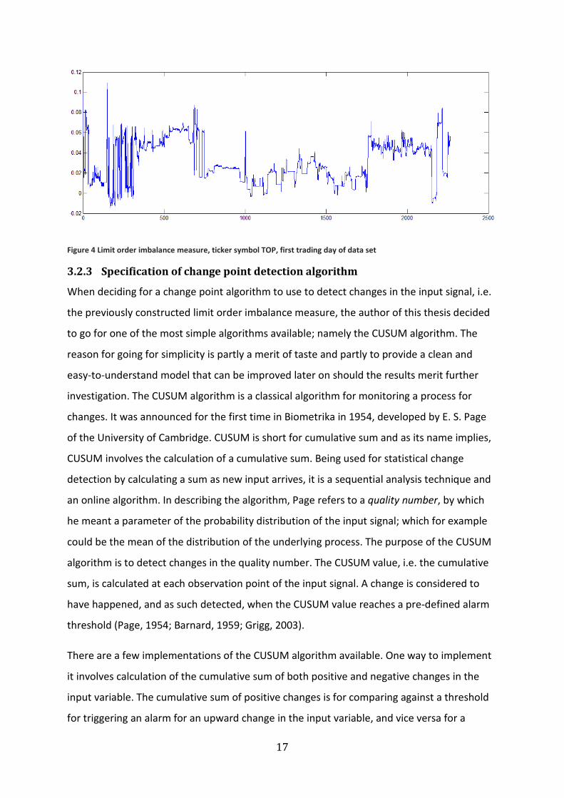
17

Figure 4 Limit order imbalance measure, ticker symbol TOP, first trading day of data set

3.2.3 Specification of change point detection algorithm

When deciding for a change point algorithm to use to detect changes in the input signal, i.e.

the previously constructed limit order imbalance measure, the author of this thesis decided

to go for one of the most simple algorithms available; namely the CUSUM algorithm. The

reason for going for simplicity is partly a merit of taste and partly to provide a clean and

easy-to-understand model that can be improved later on should the results merit further

investigation. The CUSUM algorithm is a classical algorithm for monitoring a process for

changes. It was announced for the first time in Biometrika in 1954, developed by E. S. Page

of the University of Cambridge. CUSUM is short for cumulative sum and as its name implies,

CUSUM involves the calculation of a cumulative sum. Being used for statistical change

detection by calculating a sum as new input arrives, it is a sequential analysis technique and

an online algorithm. In describing the algorithm, Page refers to a quality number, by which

he meant a parameter of the probability distribution of the input signal; which for example

could be the mean of the distribution of the underlying process. The purpose of the CUSUM

algorithm is to detect changes in the quality number. The CUSUM value, i.e. the cumulative

sum, is calculated at each observation point of the input signal. A change is considered to

have happened, and as such detected, when the CUSUM value reaches a pre-defined alarm

threshold (Page, 1954; Barnard, 1959; Grigg, 2003).

There are a few implementations of the CUSUM algorithm available. One way to implement

it involves calculation of the cumulative sum of both positive and negative changes in the

input variable. The cumulative sum of positive changes is for comparing against a threshold

for triggering an alarm for an upward change in the input variable, and vice versa for a

18

negative change. As a result, at each observation point, two CUSUM values are calculated

and then compared against a pre-defined alarm threshold. When the value of either one of

them exceeds the threshold value, an alarm is triggered and a change has thus been

detected. When a change has been detected, both cumulative sums restart from zero.

The CUSUM algorithm used in this thesis is given by the following

2345�6 � %�750, 2345� 1 16 � 7� 1 û�6

2<=5�6 � %�7 50, 2<=5� 1 16 � 7� 1 û�6

where 7� is the input signal, given by the limit order book imbalance measurement

constructed in the previous section. Thus 7� � І�. Note that 2345�6 and 2<=5�6 are the

cumulative sums at observation i for comparing against positive change threshold and

negative change threshold respectively. The initial values are given by

234506 � 0

2<=506 � 0

Lastly, û� is the estimate of the true value of the input signal and as such initially given by

the initial limit order imbalance measurement, i.e. û� � І�. Whenever either one of the

cumulative sums S?@5i6 or SBC5i6 exceeds the alarm threshold, a change point is triggered.

The input signal (i.e. the limit order imbalance measurement, which is a proxy for the shape

of the order book) is then assumed to have changed and û� is then reset to the latest limit

order imbalance value. When a change has been detected, a binary value is stored in a new

data series. A change point triggered by 234 is coded as 1 and a change point triggered by

2<= is coded as 0. All the change points form a strictly ordered sequence of binary alarms,

which later on is used in a regression to forecast price changes. Note that the resultant data

series is heterogeneous in time, i.e. there is not necessarily a strictly constant time interval

between the observations. It could e.g. be less than one millisecond, five minutes or a

completely different value between two arbitrary consecutive data points.

As long as the input signal is centered around û� and remains in control – i.e. is assumed to

not have shifted in a significant way – the CUSUM plot will show variation in a random

pattern centered above zero. If the underlying input process shifts, the CUSUM value will

19

drift upwards and eventually trigger an alarm. Below follows three examples of the CUSUM

algorithm in action processing simulated input data series. In each of the three figure pairs,

the first figure is a chart of the simulated input signal and the second figure is a chart of the

two cumulative sums 234 and 2<=. The green line is the cumulative sum tracking positive

changes in the input signal, i.e. 234. The red line is the cumulative sum tracking negative

changes in the input signal, i.e. 2<=. In other words, in these examples an upward change in

the input signal has been detected when the green line reaches the top of the chart before

resetting to zero, and a downward change in the input signal has been detected when the

red line reaches the top of the chart before resetting to zero. The first example, shown in

figure 5 and figure 6, is a series of 100 data points drawn from a normal distribution with

constant mean and constant standard deviation, followed by 100 data points where the

mean increases incrementally, followed by another 100 data points where the mean has

reverted to its initial constant value.

Figure 5 Simulated input signal; constant mean, drift in mean, constant mean

20

Figure 6 First example of the CUSUM algorithm in action

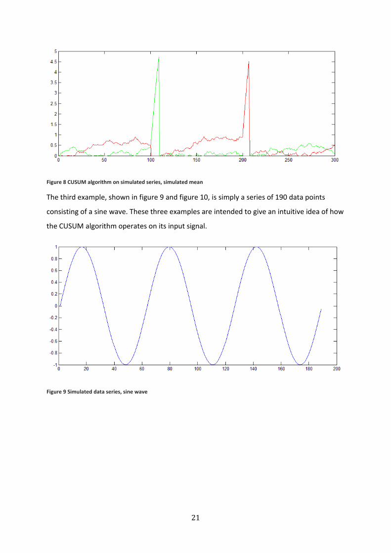
The second example, shown in figure 7 and figure 8, is a series of 100 data points drawn

from a normal distribution with constant mean and constant standard deviation, followed by

100 data points where the mean suddenly shifts upwards, followed by another 100 data

points where the mean has reverted to its initial constant value.

Figure 7 Simulated data series, sudden shift in mean

21

Figure 8 CUSUM algorithm on simulated series, simulated mean

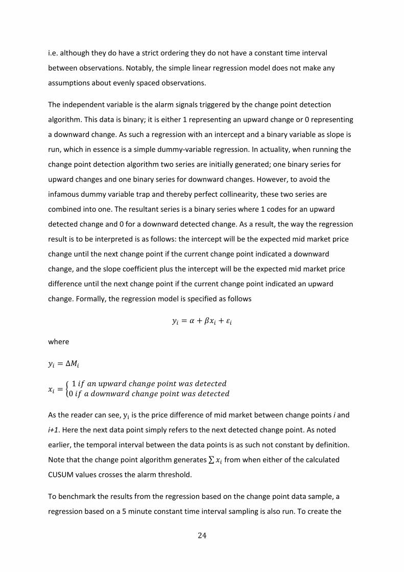
The third example, shown in figure 9 and figure 10, is simply a series of 190 data points

consisting of a sine wave. These three examples are intended to give an intuitive idea of how

the CUSUM algorithm operates on its input signal.

Figure 9 Simulated data series, sine wave

22

Figure 10 Third example of the CUSUM algorithm in action

As touched upon in the chapter covering the theoretical framework, setting the alarm

threshold is a tradeoff between false alarms, misdetections and detection delay. A false

alarm is considered to have happened when a change point was detected without an actual

change having occurred. A misdetection is considered to have happened when an actual

change has occurred but no change point was detected. Detection delay is the time between

an actual change happening and the change point being detected. To strike a balance

between these caveats, and to avoid statistical biases, the alarm threshold for each stock is

discretionary simply set to a tenth of the share price at the first available observation of

continuous trading in the data set. Across all the selected stocks during the full 20 day

sample, this on average generated roughly the same amount of change points, i.e. data

points for the regression, as a 5 minute constant time interval sampling would generate

observations. Once the alarm threshold is set, the model is ready for processing inputs.

Figure 11 and figure 12 illustrates the CUSUM value in live action processing inputs from the

data set. Figure 11 contains a series of the CUSUM value for detecting upward changes, i.e.

234. Figure 12 contains a series of the cusum value for detecting downward changes, i.e. 2<=.

The charts are based on the CUSUM value for Securitas B, ticker SECU B, during the first

trading day of the twenty day data set. Note how the CUSUM value is reset to zero

whenever the alarm threshold is crossed. As is visible in the charts, the alarm threshold is

roughly 7.5, which means that the initial share price of Securitas B during the first trading

day was roughly SEK 75. As one can see on the x-axis, there are roughly 16000 observations

of the order book during this particular day in this particular stock. Note that due to the

23

highly irregular, non linear behavior of the changes in the limit order book, the number of

observations between different trading days and different stocks can vary a lot (Cont, 2011).

Figure 11 Example of a CUSUM series for detecting an upward change

Figure 12 Example of a CUSUM series for detecting an downward change

3.2.4 Specification of regression model

Once a series of change points have been produced, it will be used as input to a regression

model that forecasts price changes. The dependant variable is the difference in mid market

from the observed data point to the next. The mid market price difference is formally

defined as follows

∆,� � ,�E- 1,�

where

,� � %�� %��$��

In other words, ∆,� is the difference of the mid market price between change point i and

change point i+1. As mentioned, the change point data series are not homogenous in time,

24

i.e. although they do have a strict ordering they do not have a constant time interval

between observations. Notably, the simple linear regression model does not make any

assumptions about evenly spaced observations.

The independent variable is the alarm signals triggered by the change point detection

algorithm. This data is binary; it is either 1 representing an upward change or 0 representing

a downward change. As such a regression with an intercept and a binary variable as slope is

run, which in essence is a simple dummy-variable regression. In actuality, when running the

change point detection algorithm two series are initially generated; one binary series for

upward changes and one binary series for downward changes. However, to avoid the

infamous dummy variable trap and thereby perfect collinearity, these two series are

combined into one. The resultant series is a binary series where 1 codes for an upward

detected change and 0 for a downward detected change. As a result, the way the regression

result is to be interpreted is as follows: the intercept will be the expected mid market price

change until the next change point if the current change point indicated a downward

change, and the slope coefficient plus the intercept will be the expected mid market price

difference until the next change point if the current change point indicated an upward

change. Formally, the regression model is specified as follows

�� F � G7� � H�

where

�� ∆,�

7� � I 1 �/ �� J�� "K��L� �� J�� "��0 �/ � ��J�J�� "K��L� �� J�� "��M

As the reader can see, y� is the price difference of mid market between change points i and

i+1. Here the next data point simply refers to the next detected change point. As noted

earlier, the temporal interval between the data points is as such not constant by definition.

Note that the change point algorithm generates ∑7� from when either of the calculated

CUSUM values crosses the alarm threshold.

To benchmark the results from the regression based on the change point data sample, a

regression based on a 5 minute constant time interval sampling is also run. To create the

25

data set used in this regression, the limit order book is simply observed once every 5

minutes. The independent variable is then at each observation calculated as the limit order

imbalance measurement, i.e. the same type of information that the change point detection

algorithm is based on. As mentioned earlier, the limit order imbalance measurement is a

scalar that represents that difference between the volume weighted average price of all limit

orders and the mid market price. The regression formula for the 5 minute interval sample is

specified as follows

�� F � G7� � H�

where

�� ∆,�

7� � І�

Thus the regression formula can be rewritten as the following

∆,� � F � GІ� � H�

where І�, as defined earlier, is the limit order imbalance measurement at observation i and

∆,� is the price difference of mid market between observation i and i+1. Here the next data

point simply refers to the next observation in the 5 minute data series. As the reader can

see, it’s a simple linear regression with an intercept and a slope. The way the regression

result is to be interpreted is as follows: the intercept will be the expected mid market price

change until the next 5 minute data point if the limit order imbalance measurement is

valued at zero. The slope coefficient will, in addition to the intercept, be the expected mid

market price difference until the next 5 minute data point if the limit order imbalance

measurement is valued at one. In essence, the regression tests the forecasting power of the

limit order imbalance measurement.

26

4 Results

This chapter contains the results from the regressions based on both the change point data

sample and on the 5 minute interval sample. A linear regression model is fitted to each stock

using data generated by the change point algorithm to forecast impending changes in mid

market. Another regression model is fitted to each stock using the limit order imbalance

measurement sampled every 5 minutes. Both data sets contain roughly the same amount of

observations over the same time period – however, the change point data set does not have

a constant time interval between the data points.

Table 1 shows the results from the regressions based on the change point data sample. The

p-value refers to the full regression model, i.e. not individual coefficients. As mentioned

earlier, the way the regression result is to be interpreted is as follows: the intercept will be

the expected mid market price change until the next change point if the current change

point indicated a downward change, and the slope coefficient plus the intercept will be the

expected mid market price difference until the next change point if the current change point

indicated an upward change. As the intuitive reasoning behind the limit order imbalance

measurement is that the price might drift up if the limit order imbalance measurement

changes upward, this implies a negative intercept and a positive slope is expected in the

regression results.

Note that the change point data sample for each stock has a different number of data points.

This is due to the fact that the change point algorithm triggers an alarm, and subsequently

generates a data point, only when the CUSUM value reaches the alarm threshold. There is

no way of knowing in advance how often this will happen.

27

Table 1 Regression results, change point sample

Symbol Number of data points in sample Intercept Slope Model p-value

KINV B 1245 -0.019 0.024 0.02

MTG B 2422 -0.053 0.083 0.00

LUPE 2318 -0.009 0.017 0.01

SECU B 1718 -0.005 0.004 0.37

GETI B 1587 -0.023 0.040 0.00

ATCO B 3046 -0.008 0.017 0.03

ELUX B 2593 -0.018 0.023 0.02

ALFA 2919 -0.016 0.024 0.00

ASSA B 3273 -0.009 0.020 0.02

SWMA 1803 -0.005 0.026 0.06

WDH 5390 -0.062 0.131 0.00

PNDORA 2038 -0.063 0.107 0.00

TRYG 2281 -0.031 0.054 0.00

GN 1071 -0.003 0.005 0.24

NKT 3175 -0.052 0.093 0.00

TOP 609 -0.114 0.216 0.11

LUN 1035 0.017 -0.014 0.31

TDC 1498 -0.004 0.005 0.01

FLS 2176 -0.064 0.130 0.00

NZYM B 776 -0.006 0.004 0.96

HUH1V 405 0.000 -0.003 0.28

CGCBV 2612 -0.006 0.013 0.00

AMEAS 1124 -0.002 0.001 0.42

KESBV 1772 -0.008 0.011 0.00

ORNBV 658 -0.001 0.001 0.60

KRA1V 1046 -0.002 0.003 0.05

OTE1V 2245 -0.006 0.013 0.00

YTY1V 1648 0.000 0.003 0.17

KCR1V 3108 -0.005 0.010 0.00

NRE1V 2263 -0.003 0.006 0.00

28

Table 2 shows a summary of the regression results based on the change point data sample.

The percentage of coefficients with anticipated signs refers to the percentage of stocks that

have estimated coefficients with signs in line with what would be expected from the intuitive

reasoning behind the model, if it has any predictive power over impending price changes.

Again, the p-value refers to the full regression model and not individual coefficients.

Table 2 Summary of regression results, change point sample

% of stocks with p-value less than 10%

70%


63%


47%

% of coefficients with anticipated signs

90%

Average number of data points per stock

1995

Table 3 shows the results from the regressions based on the 5 minute interval data sample.

The p-value refers to the full regression model, i.e. not individual coefficients. If the limit

order imbalance measurement has any predictive power over impending price changes and

the effect is in line with the intuitive reasoning behind the measurement, a positive slope

would be expected. Note that because of the constant time interval sampling of data points

the number of observations in this data sample is constant for each stock.

29

Table 3 Regression results, 5 minute interval sample

Ticker Number of observations in sample Intercept Slope Model p-value

KINV B 2020 -0.006 0.027 0.00

MTG B 2020 -0.015 -0.013 0.29

LUPE 2020 -0.003 -0.013 0.26

SECU B 2020 -0.003 -0.012 0.05

GETI B 2020 0.000 -0.021 0.04

ATCO B 2020 0.001 -0.009 0.56

ELUX B 2020 -0.015 0.187 0.00

ALFA 2020 -0.014 0.025 0.05

ASSA B 2020 0.002 -0.003 0.69

SWMA 2020 0.008 -0.010 0.29

WDH 2020 0.002 0.005 0.10

PNDORA 2020 -0.004 0.090 0.00

TRYG 2020 0.014 0.073 0.00

GN 2020 0.000 0.013 0.01

NKT 2020 -0.014 0.001 0.78

TOP 2020 -0.073 0.102 0.00

LUN 2020 0.009 0.005 0.23

TDC 2020 0.001 0.018 0.00

FLS 2020 -0.037 0.380 0.00

NZYM B 2020 -0.051 0.044 0.00

HUH1V 2020 -0.001 0.023 0.04

CGCBV 2020 -0.001 -0.002 0.86

AMEAS 2020 -0.001 -0.001 0.81

KESBV 2020 -0.002 -0.011 0.29

ORNBV 2020 0.000 -0.010 0.54

KRA1V 2020 -0.001 -0.002 0.80

OTE1V 2020 -0.001 0.076 0.00

YTY1V 2020 0.001 0.010 0.52

KCR1V 2020 0.000 -0.013 0.23

NRE1V 2020 0.000 0.009 0.71

30

Table 4 shows a summary of the regression results based on the 5 minute interval data

sample. The percentage of coefficients with anticipated signs refers to the percentage of

stocks that have estimated coefficients with signs in line with what would be expected from

the intuitive reasoning behind the model, if it has any predictive power over impending price

changes.

Table 4 Summary of regression results, 5 minute interval sample


50%


43%


33%


57%


2020

31

5 Analysis

A summary of the regression results from the two models are shown in table 5. The main

notable difference between the results of the two regressions is the difference in the

percentage of anticipated signs. In the regression based on the change point sampling, the

percentage of coefficients with anticipated signs is 90%. In other words, 27 out of the 30

stocks have estimated coefficients with signs in line with what would be expected if the

model has any predictive power over impending price changes – i.e., an upward detected

change point leads to an upward drift in price and vice versa. However the percentage of

coefficients with anticipated signs in the regression model based on the 5 minute interval

sampling is only 57%. As this is close to 50%, there is no indication as to whether a limit

order imbalance would impact the price of a stock up or down. Furthermore, the p-values

are worse across the board for the regressions based on the 5 minute interval sample.

Considering this, it is clear that the regression based on the change point data sample

performs better when forecasting impending price changes.

Table 5 Regression summary, both data samples

Change point sample regressions


70%


63%


47%


90%


1995

5 minute interval sample regressions


50%


43%


33%


57%


2020

In the results of the regressions based on the change point data sample, 70% of the stocks

have a p-value of less than 10%. This suggests that there is a certain amount of information

about impending price changes in the change point data set. Notably, 100% of the stocks

that do not have coefficient signs in line with what would be expected from the intuitive

32

reasoning behind the model have a rather high p-value. If these stocks are considered

outliers, perhaps for some reason not well fitted to the model at hand, and thereby removed

the aggregate results would be better with a higher percentage of stocks with anticipated

coefficient signs and a higher percentage of stocks with a low regression model p-value.

Notably all stocks with a relatively high p-value also have a relatively low number of

detected change points. Perhaps lowering the alarm threshold for detecting limit order

imbalance changes in these stocks would generate better regression results. Note that the

alarm threshold was set completely discretionary. To avoid statistical biases, no

optimizations were made with regards to the alarm threshold.

Only 47% of the stocks in the change point data sample have estimated regression models

with a p-value of less than 1%. However these are very significant – roughly 80% of these

have a p-value of less than 0.1%. Why some stocks show significance at the 1% level and

some not can be due to a number of reasons. As mentioned above, one of them is that the

alarm threshold of 10% of the initial stock price simply fits well with some stocks and not as

well with others. Another reason, of course, is randomness. Considering no optimizations

have been made with regards to the stock selection procedure, order imbalance measure,

alarm threshold, et cetera, there is probably room for improvement. A few ideas regarding

this will be discussed in the next chapter.

The fact that there is a different number of data points for each stock in the change point

sample is in line with the intuitive reasoning behind the model – if a sudden increase in buy

limit orders triggers a change point, this could in essence be seen as a sudden increase in

demand for the stock with an expected price increase to follow. As mentioned earlier, the

different number of observations between stocks is due to the fact that the change point

algorithm triggers an alarm, and subsequently generates a data point, only when the CUSUM

value reaches the alarm threshold. As such there is no way of knowing in advance how often

this will happen. As order arrival is a stochastic process (Cont, 2011), it makes intuitive sense

to have a stochastic number of change points unevenly spaced in time.

Note that the expected price movement after a detected change point is small. However, as

a part of a larger framework of automated liquidity provision, it still might be useful to know

that mid market is expected to rise a few cents in the near future.

33

6 Conclusion

This chapter summarizes the study. A conclusion of the thesis will be presented as well as

thoughts about future research within this subject.

6.1 Discussion of findings

The main purpose of this thesis is to propose a method using change point detection to

forecast short term limit order book price changes. Specifically, a change point detection

algorithm is used to detect what is deemed to be significant changes of the shape of the

limit order book. These detected change points are then used to forecast impending price

changes. Regression results show that the change point data contains a certain amount of

information about impending price movements. To benchmark the results, another

regression is run based on the same measurement that is used as input to the change point

detection algorithm; a limit order imbalance measurement. The main difference is that the

benchmarking regression uses constant time interval sampling of the limit order book. The

regression based on the change point data set outperforms the regression one based on a

regular time interval sampling. Overall, the results indicate that there is a certain amount of

information about impending price changes in the data series generated by the change point

detection algorithm. Even though the expected price movement after a detected change

point is small, it seems that a data set based on an online change detection algorithm might

be suitable for both practical and theoretical purposes. A potential practical use of the

results in this thesis is in the domain of automated liquidity provision. Even information

about a small impending change to the mid market price might be useful. Trading for alpha

at the highest frequency naturally converges to liquidity provision as the bid-offer spread

becomes such a major part of price changes. For theoretical purposes, if one wants to

reduce the limit order book data set for further study, it might be worth considering

sampling it using a change point detection algorithm rather than sampling it using some

arbitrary time interval. It might also be useful in the general scientific study of price

discovery and short term price formation. When studying high frequency limit order book

data sets, often times economists choose to perform a time interval based sampling of it.

This is for example done by Cao et al. (2009). When studying the limit order book, they

sample a snapshot of the first twenty price levels for both buy orders and sell orders once

every five minutes and perform regressions based on this data set. However, as the updates

34

of the limit order book is highly irregular in nature (Cont, 2011), it might preferable to use

sampling based on change point detection rather than on some arbitrary time interval if one

wants to reduce the data set for further study. There would likely be both pros and cons to

using a change point detection algorithm; however one notably pro would be that there

possibly is a higher level of information retention when sampling using change point

detection than when sampling using a constant time interval.

6.2 Suggestions for further research

As the author of this thesis found no research applying change point detection algorithm on

high frequency financial data, the model was specified as simple as possible, aiming more to

test the concept rather than optimizing for results. All measurements and models in this

thesis – the liquidity measurement, the limit order imbalance measurement, change point

detection algorithm – are constructed in this sense. As a result there is probably room for

improvement. This section covers a few ideas for further research.

There is likely room for improvement in the limit order imbalance measurement that the

change point algorithm is based on. One idea with regards to limit order imbalance

specifically is to weigh the orders based on their distance to mid market. One might assume

that orders far away from mid market might have less impact on short term price formation

than orders closer to mid market. Another idea is to base the state of the order book on

some sort of order flow. Here idiosyncrasies between various exchanges might come into

question; e.g. the prevalence of post trade-anonymity or not, as counterparty information

might potentially contribute to price formation.

The stock selection procedure could likely be improved. Price formation and asset

fundamentals might not always have a clear connection on the smallest time scale.

However, asset idiosyncrasies are still very much present in the form of various market

microstructure features such as liquidity characteristics, tick size, order priority rules etc.

Idiosyncrasies such as these might result in a difference in the price discovery process

between two assets even though they might be very similar fundamentally and even traded

on the same exchange. One example of this might be two shares from the same company

but with different voting rights and a different number of shares issued – this could in

practice result is a drastic difference in liquidity for example. The fair value of these two

35

assets is fundamentally almost the same, and the price of these two shares will by market

efficiency converge if they drift apart. However, the price formation on the very small time

scale and characteristics of the limit order book including order flow during the price

discovery process might be very different, due to the drastic difference in liquidity between

them. As a result of this, selecting stocks based on other factors such as the market

microstructure idiosyncrasies mentioned above might yield more significant regression

results. One idea is to investigate tick size. Another is to investigate average order size

resting in the order book, average time an order is resting, and average size of arriving

orders in relation to overall liquidity. Intuitively, these measures could be a proxy for the

type of participants being active in the order book, which in turn might provide information

about the price discovery process.

Different change detection algorithms can be tested; e.g. the CUSUM algorithm has different

implementations. One example of an alternative CUSUM algorithm that could be of interest

is one where a drift factor is incorporated. This factor takes into account that the parameter

value that is monitored for change might have a natural drift. Also, depending on what in the

state of the order book that is of interest, different measurements could be designed to be

used as input signal. There are also other types of change point detection algorithms that

could be of interest. Instead of deriving a simple number to represent the state of the order

book, one can use more advanced, machine learning change point detection algorithms

where the limit order book can be represented as a complete object instead of as a scalar. As

machine learning algorithms generally can have complex inputs, one does not have to derive

scalar measures of the order book to create an input. In this way there is a chance that more

information could be recovered. One idea specifically would be to try the online kernel

change detection algorithm proposed by Desobry (2005). As described, kernel change

detection compares two sets of descriptors extracted online from a signal at each point in

time. Based on a support vector machine, a dissimilarity measure in is constructed and

compared between the set in the immediate past and in the immediate future. Perhaps this

can capture features of the limit order book that otherwise might be hard to derive into a

scalar measure. In general, machine learning algorithms are able capture non-linear

relationships that other more simplistic models fail to recognize.

36

7 References

7.1 Printed sources

Y. Aït-Sahalia, P. A. Mykland, L. Zhang (2011). Ultra high frequency volatility estimation with

dependent microstructure noise. Journal of Econometrics, 160-175.

Albers, S. (2003). Online algorithms: a survey. Mathematical Programming , 3-26.

Aldridge, I. (2010). High-Frequency Trading: A Practical Guide to Algorithmic Strategies and

Trading Systems. Hoboken, NJ: John Wiley & Sons, Inc.

Barnard, G. (1959). Control charts and stochastic processes. Journal of the Royal Statistical

Society , 239–71.

C. Cao, O. Hansch, and X. Wang (2009). The Information Content of an Open Limit-Order

book. The Journal of Futures Markets, 16-41.

Cont, R. (March 2011). Statistical Modeling of High Frequency Financial Data: Facts, Models

and Challenges. Imperial College London; CNRS.

David Easley, S. H. (October 2002). Is Information Risk a Determinant of Asset Returns? The

Journal of Finance , 2185-2221.

Desobry, F. (August 2005). An online kernel change detection algorithm. IEEE Transactions

on Signal Processing , 2961-2974.

Grigg, F. V. (2003). The Use of Risk-Adjusted CUSUM and RSPRT Charts for Monitoring in

Medical Contexts. Statistical Methods in Medical Research , 147-170.

Gustafsson, F. (July 2000). Adaptive Filtering and Change Detection. West Sussex: John Wiley

& Sons, ltd.

Mark Fadiman, J. K. (2004). The evolution of trading: how technology and governance are

changing finance in the 21st Century. New York: Electronic-Boardroom TMVI Press.

Michael A. Goldstein, K. A. (April 2000). Eighths, sixteenths, and market depth: changes in

tick size and liquidity provision on the NYSE. Journal of Financial Economics , 125-149.

37

Michèle Basseville, I. V. (1993). Detection of Abrupt Changes - Theory and Application.

Englewood Cliffs, N.J.: Prentice-Hall, Inc.

Page, E. S. (June 1954). Continuous Inspection Scheme. Biometrika , 100–115.

Wilmshurst, T. H. (1990). Signal Recovery from Noise in Electronic Instrumentation (2nd ed.).

New York: CRC Press.

7.2 Electronic sources

Historical Nordic and Baltic Order Book Data (Accessed May, 2015). Retrieved from

NasdaqOMX:

http://www.nasdaqomx.com/transactions/marketdata/europeanproducts/data-

products/nordic-historical-view

38

8 Appendix

8.1 Source code

The code used for extracting and analyzing the data for this thesis is written in MatLab and

will be made available upon request.

forecasting limit order book price changes using change...

Documents