forecasting mortality rates via density ratio … mortality rates via density ratio modeling...

Thc Canadian Journal of Statistics Vol. 36, No. 2,2008, Wges I9S206 La revue canadienne de statistique

193

Forecasting mortality rates via density ratio modeling Benjamin KEDEM, Guanhua LU, Rong WE1 and Paul D. WILLIAMS

Key wonls andphrases: Age-specific mortality; autoregression; combined data; forecasting; one-year ahead forecast; predictive distribution; semiparametric method.

MSC 2000: Primary 62M20; secondary 62GO7.

Abslruct: The authors propose a semiparametric approach to modeling and forecasting age-specific mortality in the United States. Their method is based on an extension of a class of semiparametric models to time series. It combines information from several time series and estimates the predictive distribution conditional on past data. The conditional expectation, which is the most commonly used predictor in practice, is the first moment of this distribution. The authors compare their method to that of Lee and Carter.

Prevision de taux de rnortalite par la rnodelisation d’un rapport de densites Rburnt : Les auteurs proposent une methode semiparamktrique pour la modelisation et la prevision de la mortalit6 par tranche d‘tiges aux fitats-Unis. Leur approche s’appuie sur la generalisation d’une classe de modbles semiparametriques au cas de series chronologiques. Elle exploite l’information provenant de plu- sieurs series et estime la loi pr&ictive ?I partir du comportement passe. L’esp6rance conditionnelle, qui sert le plus souvent de predicteur en pratique, en est le premier moment. Les auteurs comparent leur mdthode h celle de Lee et Carter.

1. INTRODUCTION Since 1900, the United States Government has been collecting mortality data from death registra- tion records assembled by state vital statistics offices. The data are broken down mainly by state, cause, race, gender, and age, and are published in the form of death rates and life expectancies decennially and/or annually for over 100 years. However, the existing electronically documented mortality data are relatively short. In this study we shall use well documented mortality time series from 1970 to 2002 to forecast mortality patterns in the U.S. This gives us relatively short annual age-specific time series, consisting of a little over 30 observations each, stratified by fac- tors such as state, gender, and race. Prediction of future annual death rates based on these time series must take into account their short length.

The objective of the present study is to forecast mortality patterns, using relatively short historical time records, by following a two-stage procedure. First, to each short series we fit a first order autoregressive model, and then, to overcome the problem of short series, the resulting residuals are combined or merged in some fashion to provide estimates of future predictive distributions. Point forecasts, such as the conditional expectation, are obtained as a byproduct.

In this paper we apply a semiparametric forecasting method advanced recently in Kedem, Gagnon & Guo (2005). The method compensates for short individual records by combining them via a density ratio model as described in Section 2. Accordingly, the residuals from several different fitted models are combined in this way in order to estimate the entire future conditional distributions of interest. From this we obtain future conditional probabilities as well as the conditional expectation of future values given past information, the most common predictor. We focus primarily on the prediction of centered annual age-specific log-death rates for the entire U.S. using data from 1970 to 2002.

1.1. U.S. mortalityrate data.

The death or mortality rate for age x and year t is the number of people who died at age x during

KEDEM, LU, WEI, &WILLIAMS Vol. 36, No. 2 194

year t divided by the number of people of age x at the beginning of year t. It is customary to report death rate on a (natural) logarithmic scale. Our data structure has the form of log-death rate denoted as m(x, t) for ages z = I, . . . ,85, and year t = 1971, . . . ,2002.

Comparison of Log Death Rate Curves for Years

N

P

Y s 6 I 0

- 8'9

?

0 20 40 80

age

FIGURE 1 : Log-death rate m(x, t ) as a function of age x for some fixed t.

The plot of m(x, t) as a function of age x resembles a pointed hook with a rather long handle, surprisingly similar to a dentist probe, as seen from Figure 1. Wei, Curtin & Anderson (2003) fitted to these data the eight parameter model of Heligman & Pollard (1980), demonstrating that the model captures well the pointed hook pattern of mortality versus age. Figure 1 also shows that the hook pattern repeats itself year after year persistently, and that in general annual death rates decline, again quite persistently. The decline in death rate for fixed age as a function of time is shown in Figure 2 on a log-scale for several ages. Except for age 0, these time series appear almost as parallel straight lines, but when drawn separately they are much more oscillatory.

Age-specific Time Series of Log Death Rates

- - - .- - .- - - - - -

~

-- -. . - -

age 10 age 20 age 50 age 60

- _ _ _ _ _ _ - , - - .. -

9 1970 1975 1980 1985 1990 1995 2000

Year

FIGURE 2: Age-specific time series m(x, t ) for some fixed x.

2008 DENSITY RATIO MODELING 195

2-

x -

2-

9- 0

:- t 9-

Let d(x, t) denote the centered log-death rate matrix, d(z, t) = m(x, t ) - c, m(x, t) /n. We model d(z, t) instead of m(z, t) in order to compare our method with that of Lee & Carter (1992) who also use centered data. Plots of d(x,t) are shown in Figure 3 as a function of x for some fixed t, and also as a function o f t for various fixed ages x. From the plots we see that neighboring time series d(z, t) and d(x’, t), where z and x’ are close, e.g. ages 60 and 61, behave quite similarly. To compensate for short time records, the semiparametric method combines information from several agewise neighboring time series.

Centered Year-Specific Log Death Rate Curves

I

I

. . . . ;. - -.\ - . . .. . . . .. . .

- I , ,’

I I I I I I I I I

0 1 0 2 0 3 0 4 0 5 0 8 0 7 0 8 0

age

Centered Age-specific Time Series of Log Death Rates

1970 1975 1980 198.5 1995

Year

FIGURE 3: Plots of centered log-death rates d(z , t ) as a function of 2 for fixed t (top) and as a function of t for fixed x (bottom).

1.2. The Lee-Carter model.

The model proposed by Lee & Carter (1992) is used by the U.S. Census Bureau as a bench- mark for their population forecasts, and its use has been recommended by the two most recent U.S. Social Security Technical Advisory Panels. It also appears to be the dominant method in the academic literature and is used widely by scholars forecasting all-cause and cause-specific

196 KEDEM, LU, WEI, 81 WILLIAMS Vol. 36, No. 2

mortality around the world. See Lee (2000) and Lee & Miller (2001). The Lee-Carter model is based on principal components. If m denotes the number of mortality time series, each corresponding to a specific age, the Lee-Carter model searches for the first principal component in m dimensional time series data, and solves for the age and time parameters by using singular value decomposition.

The method presented in this paper is very different and seems appropriate for short range forecasting. Both methods, however, are extrapolative in that future mortality rates are estimated from past rates. Lee & Carter (1992) employed tabulated mortality data available from 1900 to 1987. However we shall compare the two methods using the annual data systematically collected from 1970 to 2002.

2. AN APPROACH TO SEMIPARAMETRIC TIME SERIES FORECASTING

Our approach for tackling the problem of short time series is based on a certain “tilt” model studied in several works including Fokianos, Kedem, Qin & Short (2001), Gilbert, Lele & Vardi (1999), Qin (1993), Qin (1998), Qin & Zhang (1997), and Vardi (1982, 1985).

In what follows next, zjt denotes the j th time series depending on covariate vector zj t

through model fj.

2.1. The density ratio model.

Consider the following m = q + 1 time series regressions,

Xlt = f l ( z l , t - l ) + E l t , t = 1 ,... ,n1,

zqt = fq(.q,t-l) +Eqt, t = 1 ,..., nq, zmt = fm(Zrn, t - l ) + E d t = 1 ,..., n,,

where the ni are small, the vectors z ~ , ~ - I contain past values of covariate time series, and &kt are independent noise components. Since &kt cannot be used directly for estimation, our proposed strategy is to first fit model (1) and then use the residuals ekt wherever Ekt are required.

Suppose the Ekt have probability densities,

Define the reference density g ( z ) = gm(z) with G(z) = G,(z) the corresponding cumulative distribution function. Then we shall assume the density ratio model relative to the reference g(z),

7 4- (3)

This in turn gives the tilt model

with a normalizing constant a3, vector ,Bj, and a vector valued distortion or tilt function h(z) . Implicitly, crj is a function of &. The distorted densities g j , the reference g , as well as the aj and Pj are all unknown, but the distortion function h(z) is assumed to be known and its choice depends on the data.


An important special case of (3) is obtained in the normal case. Assume that z1 - N(p1, u?) and 2 2 N N ( p 2 , ug) with densities g1 and 92 , respectively. Then the density ratio (3) becomes

with a and P = ( P I , P2)T depending on the normal parameters,

and a two dimensional distortion function h(z) = (z, z2)T. Notice that h(z) degenerates to z2 when 111 = ~2 = 0, and ( 5 ) reduces to

g 1 ( z ) = ea+Pz2g2(z) (6)

with scalars a, P. The tilt model (6) is useful when the distributions are centered at zero and are symmetric.

2.2. Estimation. Combine all the residuals from the q + 1 regressions into a single vector of length n = n1 + * * * + nq + nm,

(7)

Maximum likelihood estimates for the aj , / I j , and G ( z) can be obtained from the entire vector of residuals (7) by maximizing the likelihood over a class of step cumulative distribution functions with jumps at the values el, . . . , en. Let pi = dG(e+) denote the probability of jump at point e+. Then the semiparametric likelihood becomes

T e = ( e l , . . . , en)T = ( ( e l l , . . . , eln,) , . . (eql , . . . , eqnq ), (em1 , . emn, )) .

The likelihood (8) is sometimes referred to as empirical likelihood. To maximize the likelihood (8) we follow a profiling procedure used in Fokianos, Kedem, Qin & Short (2001). First, fix the a and P. Then, subject to the normalization constraint C r = l pi = 1, and the constraints induced by the tilt model (4)

n

C p , [ e x p { c y , + ~ , T h ( e i ) ) - 11 = 0, j = 1,. . . , q, i=l

the pi which maximize (8) are given by

1 1 p . = ( p)=- nm 1 + p1 exp{al+ P:h(ei)) + * * + pq exp{aq + P,Th(ei)) 2 -Pi 0,

where p3 = n3/nmr j = 1,. . . , q, are the relative series sizes. The final solution for the pj is

(9)

obtained by substituting p i ( a , P) back into the likelihood (8) and finding maximum likelihood estimators ii3 and fi3 through profiling. With I ( B ) the indicator of the event B, the estimated

1 1 $2 = G 1 + p1 exp{&1+ pTh(e,)) + * - + pq exp{&, + f i z h ( e + > )

198 KEDEM, LU, WEI, &WILLIAMS Vol. 36, No. 2

reference cumulative distribution function is given by

i = l

Smoothing the $i in (9) by a kernel or, alternatively, smoothing increments of G ̂in (10) gives the reference density estimate g (Fokianos 2004).

The main point of the semiparametric paradigm discussed here is that the reference cumulative distribution function G(z) is estimated from many samples giving an improved estimate as compared with the empirical cumulative distribution function which is obtained from the reference sample only. This fact has been addressed carefully by several authors. In particular, very general optimality properties of the semiparametric estimates are discussed rigorously in Gilbert (2000). Let en = (&I, . . . , Liq, 81,. . . , fiq)'. Then, as Gilbert (2000) has shown, (en, G^) are asymptotically normal and efficient. Likewise, Zhang (2000b) has shown that quantile estimates obtained by the semiparametric method from both case and control samples are more efficient than estimates that are based on the control sample only, ignoring the case information. More recently, Fokianos (2004) showed that by merging information following the semiparametric paradigm, we obtain improved kernel density estimates with the same bias as the traditional kernel density estimates but with smaller asymptotic variance. Our data analysis below supports this claim. Moreover, merging information in this way can result in power- ful tests for distribution equality. See Fokianos, Kedem, Qin & Short (2001), Gagnon (2005), and Kedem & Wen (2007). Regarding the uncertainty in G^, as shown by Zhang (2000b) and more recently by Lu (2007), fi (e - G) converges to a Gaussian process with mean zero and a rather complex covariance structure. In addition, it can be shown that the estimates h and f i are asymptotically normal with a covariance structure depending on functionals of G; see Fokianos, Kedem, Qin & Short (2001), Kedem & Wen (2007), Lu (2007), Qin & Zhang (1997), and Zhang (2000a).

We shall apply the semiparametric paradigm in forecasting U.S. mortality rates by combining information, or borrowing strength, from several (agewise) neighboring short U.S. mortality time series,

2.3. Forecasting. The preceding discussion motivates the following time series forecasting method (Kedem, Ga- gnon & Guo 2005). Since ~ , , ~ + l = fm(zm,t) + ~~,~+_+l, and E m , t f l N G, where G is the reference distribution estimated semiparametrically by G as in (lo), we estimate the predictive distribution at time t + 1 conditional on past data z,,t as follows:

All sorts of point predictors can be obtained from (1 1). In particular, a one-step ahead predictor for ~ , , ~ + l given the past can be approximated by calculating the (conditional) mean of the shifted distribution C(z - fm(zm, t ) ) . Approximate prediction intervals can also be obtained from the estimated distribution (1 1).


2.4. About independence. Strictly speaking, the method as outlined above requires independent noise components &ktr but since the Ekt are replaced by the corresponding residuals in practice, strict independence is not guaranteed. The question is then whether the independence requirement may be relaxed.

In Kedem & Fokianos (2002) it was shown that, subject to some regularity conditions, by using partial likelihood it is possible to bypass independence and extend the generalized linear models methodology to dependent time series. With this in mind, if the likelihood (8) is inter- preted in a partial sense, then this suggests the method may still be viable even when residuals are used, as is evident from the present application to mortality rates forecasting, and another very different application to filtered mortality time series reported in Kedem, Gagnon & Guo (2005).

More directly, the independence question was investigated in Kedem, Gagnon 8t Guo (2005) by means of an extensive simulation applied to the bivariate linear system

zt = a 1 z t - 1 + a2gt-1 + E t ,

Yt = h z t - 1 + b2gt-1 + vt,

t = 1,. . . , N, with independent Gaussian noise components E t N N(0, of) and vt N N(0, oz) satisfying the density ratio model with

Then, estimating G when all the parameters in (12) and (13) were known and using known independent noise components ~ t , vt, and also when all the parameters were estimated (onse with N = 50 and once with N = 500) and using residuals it, 7j t , gave nearly the same G, and hence nearly identical forecasts. This suggests that there are situations where the quality of prediction of the semiparametric method is not necessarily affected much by the use of the observed residuals.

3. ONE YEAR AHEAD PREDICTION OF U.S. MORTALITY

3.1. A two-stage procedure. Define ak = ct m(k, t)/n. As mentioned above, we analyze the centered log-death rate matrix d ( k , t), d(k, t ) = m(k, t) - ak. For each fixed age k, consider the annual time series of centered log death-rates from 1970 to 2001. Thus t = 1, . . . ,32.

Write z k t = d(k, t ) . First, to each such time series we fit the first order autoregressive model with drift c k ,

(14)

The drift parameter is added in order to capture a downward trend observed in the age-specific centered log death-rate time series as exemplified in Figure 3. Accordingly, the functions fk in the system (1) are given by fk(Zk,t- l ) = bkzk,t-1 + c k . The coefficient bk and the drift c k are estimated by least squares, and in our application the &kt are replaced by the residuals derived from the model (14).

Next, we choose a density ratio model for the residuals. Data analysis shows that the residuals corresponding to model (14) are centered around zero and that their histograms resemble those obtained from small normal samples. This motivates the distortion model (6) with h(z) = z2.

We consider the mth residual sample (e,l, . , . , emn,) as the reference where each component has distribution function G and density g. Similarly, assume that each residual component of the vector ( e k l , . . . , e k n k ) has distribution Gk and density gk, k = 1, . . . , q. Following the above semiparametric paradigm, and combining it with insight gained from histograms of residuals from (14), we assume the density ratio relationship,

z k t = & z k , t - l + ~k + E k t , k = 1,. . . , q, m.

gk(z) = eak+fl*x2 g(z), k = 1 ,..., q. (15)


An application of the semiparametric procedure to the combined data e defined by (7) gives the semiparametric estimate for the reference distribution. Similarly, from (10) and (15) we obtain the estimated distribution function of the kth sample from which the predictive distribution is computed by

h

P ( zk , t+ l I z I ~ k t ) M Gk(z - h Z k t - ck) . (16)

3.2. Data analysis.

We consider 85 age-specific time series of log-death rates (all-cause) for ages 1, . . . ,85, where the age category 85 includes ages 85 and older. To simplify the analysis, this grouping or lumping of ages 85 and older had to be done at some point and we chose, somewhat arbitrarily, age 85 as a threshold. However, the data file does have the specificity to subpartition this category to obtain a more detailed mortality prediction. Mortality at age 0 is not considered in the present analysis due to its behavior which is very different from that at other ages. See Figure 2.

From the previous discussion, the assumption that the density ratio model (15) holds for time series groups corresponding to neighboring ages seems reasonable. Indeed, in retrospect our data analysis lends credence to this assumption. In our analysis, therefore, we apply the semiparametric method by combining information from each of the age groups, consisting of five ages each and dubbed “Sage,” 1-5, 6-10, . . ., 81-85, a total of 17 groups, where the time series “in the middle” of each group is taken as the reference. For example, in the group 1-5, the time series of age 3 is taken as the reference, meaning that the relevant distribution from this time series serves as the reference distribution for the group. We applied the semiparametric model separately to each group to estimate the reference distribution and the corresponding distorted distributions to obtain predicted mortality curves.

As an illustration, consider the age group 31-35 from 1970 to 2001. As mentioned before, we chose a quadratic distortion function h(z) = x2 due to the rough symmetry of the residuals around zero, resembling the behavior of normal residuals. There are altogether five residual samples, and the sample of residuals from age 33 is considered as the reference. The actual conditional point predictions of log death-rate in 2002 for the age group 31-35-are obtained from (16) by computing the-first moments of the shifted predictive distributions Gk, k = 31, . . . ,35, respectively, with G33 as the reference. This analysis is repeated for all 17 groups. The 2002 prediction results for all ages are compared with the true 2002 centered log-rates in the tables and figures below.

0 1 5 O W O M 00 O M 0 10 0 1 5 010 001 0 0 OM OIO

FIGURE 4: Estimated reference probability density function of age 33 from the combined data e for the 3-age group 32-34 (left), and the 5-age group 31-35 (right), respectively.

It is also interesting to compare the results from the 3-age group 32-34 with the 5-age group 31-35. Figure 4 shows the histograms and overlaid estimated reference density of age 33 ob-


tained from the combined data e for the 3-age and 5-age groups. Since we combined more information in the 5-age group there is a noticeable improvement in the density fit.

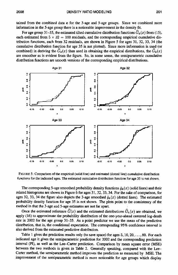
For age group 31-35, the estimated tilted cumulative distribution functions e k ( z ) from (19, each estimated from 5 x 32 = 160 residuals, and the corresponding empirical cumulative distribution functions, each from 32 residuals, are shown in Figure 5 for ages 31, 32, 33, 34 (the cumulative distribution function for age 35 is not plotted). Since more information is us2d (or combined) in deriving the ek(z) than used in obtaining the empirical distributions, the Gk(z) are smoother as is evident from the figure. So, in some sense, the semiparametric cumulative distribution functions are smooth versions of the corresponding empirical distributions.

Age 31 Age 32

-0.15 -0.10 -0.05 0.0 0.05 0.10 -0.15 -0.10 -0.05 0.0 0.05 0.10

x X

Age 33 Age 34

- r

x -0.15 -0.10 -0.05 0.0 0.05 0.10 -0.15 -0.10 -0.05 0.0 0.05 0.10

X X

FIGURE 5: Comparison of the empirical (solid line) and estimated (dotted line) cumulative distribution functions for the indicated ages. The estimated cumulative distribution function for age 35 is not shown.

The corresponding Sage smoothed probability density functions gk(z) (solid lines) and their related histograms are shown in Figure 6 for ages 31,32,33,34. For the sake of comparison, for ages 32, 33, 34 the figure also depicts the 3-age smoothed gk(z) (dotted lines). The estimated probability density function for age 35 is not shown. The plots point to the consistency of the method in that the 3-age and 5-age estimates are not far apart.

Once the estimated reference e(z) and the estimated distributions z k ( z ) are obtained, we apply (16) to approximate the probability distribution of the one-year-ahead centered log-death rate in 2002 for the age group 31-35. As a point predictor we use the mean of the predictive distribution, that is, the conditional expectation. The corresponding 95% confidence interval is also derived from the estimated predictive distribution.

Table 1 gives the prediction results only (to save space) for ages 5,10,20,. . . ,80. For each indicated age it gives the semiparametric prediction for 2002 and the corresponding prediction interval (PI), as well as the Lee-Carter prediction. Comparison by mean square error (MSE) between the two methods is given in Table 2. Generally speaking, compared with the Lee- Carter method, the semiparametric method improves the prediction as measured by MSE. The improvement of the semiparametric method is more noticeable for age groups which display


more steady and gradual change of death rate as in age groups 3 1-50 and 7 1-85. From Table 2, the overall prediction MSE from the semiparametric method in the three cases reported there are 0.104,O. 187,0.249, compared, respectively, to 0.297,0.619,0.645 from the Lee-Carter method. The most significant improvement is for the age groups 3 1-50 and 71-85, whereas both methods perform quite similarly for all other age groups as we see from the table.

Age 31 Age 32

0 1 5 0 1 0 005 0 0 005 010 015 0 1 5 0 1 0 005 0 0 005 010

X X

Age 33 Age 34

0 1 5 0 1 0 0 0 5 0 0 005 010 0 1 5 0 1 0 005 0 0 005 010

x x

F I G U R E 6: Histograms and overlaid estimated probability density functions for 3-age group 32-34 (dotted line) and 5-age group 31-35 (solid line). The estimated probability density function for age 35 is not

shown.

In the above data analysis we combined information from non-overlapping 5-age groups. The analysis was repeated for the general poulation case by using a sliding window of overlapping 5- age groups, each time moving up by a single year. Interestingly, the MSE results were very close to those reported in Table 2, replacing the SP row 0.104, 0.050, 0.015, 0.030, 0.009 by 0.105, 0.051, 0.014, 0.031, 0.008. This suggests that the choice of the reference time series within an age group may be arbitrary.

TABLE 1 : Prediction comparison between the semiparametric and Lee-Carter methods for 2002 for some ages. The first two rows give the 95% PI bounds for the semiparametric forecasts, and the rest are the

predictions from the semiparametric method (SP), true values in 2002, and the prediction from the Lee-Carter (LC) method.

Age 5 10 20 30 40 50 60 70 80

Lower -8.781 -8.933 -7.072 -6.977 -6.276 -5.473 -4.628 -3.776 -2.905

Upper -8.599 -8.671 -6.870 -6.755 -6.094 -5.362 -4.557 -3.695 -2.774

True -8.639 -8.785 -6.970 -6.868 -6.172 -5.416 -4.622 -3.733 -2.824 SP -8.699 -8.819 -6.997 -6.858 -6.178 -5.431 -4.601 -3.749 -2.842

LC -8.661 -8.835 -7.023 -6.810 -6.252 -5.534 -4.615 -3.752 -2.874

From Table 2, we see that the MSE from the semiparametric method is lower for the general population case than in both the female and white female cases. This is not surprising since

2008 DENSITY RATIO MODELING

more data are available from the total population, whereas in the other two cases we deal with subpopulations. The fact that the age group 1-30 has a larger MSE than that from the other groups is due to the large variation of the data associated with that age group.

Since our mortality data are truncated at age 85, we cannot calculate traditional life tables from the death rate forecasts. Instead we provide in Table 3 a comparison between the true and predicted (by our method) number of survivors by age and sex out of 100,000 live births. The true values and their forecasts are close.

TABLE 2: Mean square error of (all-cause) prediction from the semiparametric (SP) and Lee-Carter (LC) methods for the general population, female, and white female.

Agegroup 1-85 1-30 31-50 51-70 71-85

General SPmodel 0.104 0.050 0.015 0.030 0.009 LCmodel 0.297 0.078 0.180 0.026 0.013

Female SPmodel 0.187 0.121 0.026 0.032 0.008 LCmodel 0.619 0.226 0.341 0.027 0.025

W. Female SPmodel 0.249 0.176 0.031 0.033 0.007 LCmodel 0.645 0.257 0.329 0.041 0.019

4. TWO-YEAR AHEAD FORECASTING

So far we have discussed one-year ahead prediction. However, our one-step procedure can be extended to multi-year ahead forecasting. One way to proceed is to use the predicted values from previous steps when making long term predictions. Thus in two-year ahead forecasting we use the previous one-year ahead forecasts, and proceed as above. The prediction error may get amplified through each additional step even if minor deviations of prediction from true values occur. The results from this procedure are reported in Table 4(a). Again, the overall MSE is lower for the semiparametric method as compared with the Lee-Carter method.

A second procedure for forecasting j-years ahead is to extend the above one-step ahead forecasting method to residuals resulting from time series regression models where the present at time t is regressed on observed values up to and including t - j. Thus in the present case, to get two-year ahead mortality forecasts we use (14) with the modification that x k t is regressed on Z k , t - 2 . The MSE from this method is reported in Table 4(b). Once more, the overall MSE is lower for the semiparametric method as compared with the Lee-Carter method. The disadvan- tage of this procedure is that some data are lost due to the larger time lags.

5. CONCLUDING REMARKS We have used a two-stage forecasting semiparametric procedure suitable for short time series to obtain forecasts of U.S. age-specific mortality rates. To estimate conditional predictive distributions, the method combines short time series by appealing to a density ratio model. Point predictors as well as future probabilities can be obtained from the estimated conditional distributions. A comparison with the well known Lee-Carter singular value decomposition method points to the potential of the semiparametric method. In general the semiparametric method provides more precise short term prediction as compared with the Lee-Carter procedure.

The method we used is non-Bayesian. Bayesian methods for forecasting in short time series are available, a useful special case of which is discussed by De Oliveira, Kedem & Short (1997), and Kedem & Fokianos (2002). Interestingly, there too the prediction is based on a predictive distribution, but the method is very different.


Death rates drop rapidly from infants to children, thus, combining data from age zero with other ages to form an age group is less appealing. It seems preferable to employ methods suitable for univariate time series to forecast the annual mortality for age zero. When monthly infant death rates are available, the semiparametric method can be applied to this age group separately.

TABLE 3: Number of survivors by age and sex, out of 100,000 born alive, from both semiparametric forecasts and true values in 2002.

Forecast True Age Total Male Female Total Male Female 0 I00000 1 99311 5 99182

10 99107 15 99013 20 98685 25 98219 30 97746 35 97189 40 96384 45 95231 50 93558 55 91205 60 87762 65 82616 70 75218 75 65081 80 51665 85 35348

lo0000 9923 1 99085 99004 98890 98425 97717 9703 1

96275 9522 1 93739 91581 88625 84429 78258 69571 57967 43306 26897

1 ooooo 9937 1

99256 99 186 99108 98914 98679 98394 98012 97425 96550 95293 93446 90632 86313 79978 71052 58630 42244

1 oooO0 99298 99174 99098 99000 98662 98192 97722 97171 96386 95216 93515 91 I28 87629 82484 75148 65014 5 1680 35442

1 ooooo 992 17 99076 98992 98875 98400 97691 97006 96249 95228 93733 91553 88521 8421 1 77986 69339 57710 43142 26938

1OOOOO 99360 99252 99 184 99104 98902 98662 98384 98009 97422 96520 95220 93381 90570 86328 80074 71164 58758 42330

For convenience, we chose to fit to the mortality rate time series the AR( 1) model (14). This of course is only one possibility and there are other choices. For example, we could set the coefficient bk in (14) to be 1, or use an AR(2) model. A model which provides a better fit could reduce the prediction error.

TABLE 4: Prediction MSE from the semiparametric (SP) and Lee-Carter (LC) methods for two-year ahead forecasting. (a) Predicted one-year ahead forecasts are used. (b) Autoregression lagged by 2.

Agegroup 1-85 1-30 31-50 51-70 71-85

(a) SPmodel 0.180 0.128 0.019 0.026 0.007 LC model 0.389 0.088 0.246 0.033 0.021

(b) SPmodel 0.211 0.132 0.048 0.025 0.005 LC model 0.389 0.088 0.246 0.033 0.021


ACKNOWLEDGEMENTS The authors would like to thank the reviewers and several colleagues at the National Center for Health Statistics for useful comments and suggestions which have been incorporated in the paper. This work was supported by CDCNCHS.

REFERENCES V. De Oliveira, B. Kedem & D. A. Short (1997). Bayesian prediction of transformed Gaussian random

K. Fokianos (2004). Merging information for semiparametric density estimation. Journal of the Royal

K. Fokianos, B. Kedem, J. Qin, & D. A. Short (2001). A semiparametric approach to the one-way layout.

R. E. Gagnon (2005). Certain Computational Aspects of Power Effciency and State Space Models. Doctoral

P. B. Gilbert (2000). Large sample theory of maximum likelihood estimates in semiparametric biased

P. B. Gilbert, S. R. Lele & Y. Vardi (1999). Maximum likelihood estimation in semiparametric selection

L. Heligman & J. H. Pollard (1980). The age pattern of mortality. Journal of the Institute of Actuaries,

B. Kedem & K. Fokianos (2002). Regression Models for Time Series Analysis. Wiley, New York. B. Kedem, R. E. Gagnon & H. Guo (2005). Time Series Prediction Via Density Ratio Modeling. Unpub-

lished manuscript, Dept. of Mathematics, University of Maryland, College Park. B. Kedem & S. Wen (2007). Semi-parametric cluster detection. Journal of Statistical Theory and Practice,

1,49-72. R. Lee (2000). The Lee-Carter method for forecasting mortality, with various extensions and applications.

North American Actuarial Journal, 4,8043. R. D. Lee & L. R. Carter (1992). Modeling and forecasting U.S. mortality. Journal of the American

Statistical Association, 87,659-67 1. R. Lee & T. Miller (2001). Evaluating the performance of the Lee-Carter approach to modeling and fore-

casting mortality. Demography, 38,537-549. G. Lu (2007). Asymptotic Theory for Multiple-Sample Semiparametric Density Ratio Models and its Appli-

cation to Mortality Forecasting. Doctoral dissertation, Dept. of Mathematics, University of Maryland, College Park.

fields. Journal of the American Statistical Association, 92, 1422-1433.

Statistical Society Series B, 66, 941-958.

Technometrics, 43,56-65.

dissertation, Dept. of Mathematics, University of Maryland, College Park.

sampling models. The Annals ofdtatistics, 28, 151-194.

bias models with application to AIDS vaccine trials. Biometrika, 86,2743.

107,659-671.

J. Qin (1993). Empirical likelihood in biased sample problems. The Annals OfStatistics, 21, 11 82-1 196. J. Qin (1 998). Inferences for case-control and semiparametric two-sample density ratio models. Biometrika,

J. Qin & B. Zhang (1997). A goodness of fit test for logistic regression models based on case-control data.

Y. Vardi (1982). Nonparametric estimation in the presence of length bias. The Annals of Statistics, 10,

Y. Vardi (1985). Empirical distribution in selection bias models. The Annals ofstatistics, 13, 178-203. R. Wei, R. L. Curtin & R. Anderson (2003). Modeling U.S. mortality data for building life tables and further

B. Zhang (2000a). M-estimation under a two sample semiparametric model. Scandinavian Journal of

85,619-630.

Biometrika, 84,609-618.

616-620.

studies. 2003 Joint Statistical Meeting Pmceedings, Biometrics Section, 458-4464.

Statistics, 27, 263-280.


B. Zhang (2000b). Quantile estimation under a two-sample semi-parametric model. Bernoulli, 6,491-51 1 .

Received 21 May 2007 Accepted 5 November 2007

Benjamin KEDEM: [email protected] Guanhua LU: [email protected]

Department of Mathematics University of Maryland

College Park, MD 20742, USA

Rong WEI: [email protected] Paul D. WILLIAMS: [email protected]

Ofice of Research and Meihodology National Center for Health Statistics

Hyattsville, MD 20782, USA

forecasting mortality rates via density ratio … mortality rates via density ratio modeling...

Documents