forecasting office space demand - naiop

Hany Guirguis, Ph.D.Professor, Economics-FinanceManhattan CollegeRiverdale, New York

Joshua Harris, Ph.D., CRE, CAIADirector, Dr. P. Phillips Institute for Research and Education in Real EstateUniversity of Central FloridaOrlando, Florida

Forecasting Office Space Demand

© 2016 NAIOP Research Foundation

This report is protected by copyright and may not be reproduced or redistributed in whole or in part, in print or any digital form, without the express written consent of the publisher. To obtain permissions, please contact Margarita Foster (see below).

There are many ways to give to the Foundation and support projects and initiatives that advance the commercial real estate industry. If you would like to do your part in helping this unique and valuable resource, please contact Bennett Gray, senior director, at 703-904-7100, ext. 168, or [email protected].

Requests for funding should be submitted to [email protected]. For additional information, please contact Margarita Foster, NAIOP Research Foundation, 2201 Cooperative Way, Suite 300, Herndon, VA 20171, at 703-904-7100, ext. 117, or [email protected].

Prepared for and Funded by the NAIOP Research Foundation

By

Hany Guirguis, Ph.D.

Professor, Economics-Finance

Manhattan College

Riverdale, New York

Joshua Harris, Ph.D., CRE, CAIA

Director, Dr. P. Phillips Institute for Research and

Education in Real Estate

University of Central Florida

Orlando, Florida

January 2016

Forecasting Office Space Demand

About NAIOPNAIOP, the Commercial Real Estate Development Association, is the leading organization for developers, owners, investors and related professionals in office, industrial, retail and mixed-use real estate. NAIOP comprises some 17,000 members in North America. NAIOP advances responsible commercial real estate development and advocates for effective public policy. For more information, visit naiop.org.

About the NAIOP Research Foundation

The NAIOP Research Foundation was established in 2000 as a 501(c)(3) organization to support the work of individuals and organizations engaged in real estate development, investment and operations. The Foundation’s core purpose is to provide these individuals and organizations with the highest level of research information on how real properties, especially office, industrial and mixed-use properties, impact and benefit communities throughout North America. The initial funding for the Research Foundation was underwritten by NAIOP and its Founding Governors with an endowment fund established to fund future research. For more information, visit naioprf.org.

About the Researchers Hany Guirguis is a professor in the department of economics-finance at Manhattan College in New York.

Joshua Harris is a lecturer of finance and real estate and director of the Dr. P. Phillips Institute for Research and Education in Real Estate at the University of Central Florida in Orlando, Florida.

Contents

Executive Summary . . . . . . . . . . . . . . . . . . . . . . . . . . . . . . . . . . . . . . . . . . 1

The Model . . . . . . . . . . . . . . . . . . . . . . . . . . . . . . . . . . . . . . . . . . 1

The Results and the Product . . . . . . . . . . . . . . . . . . . . . . . . . . . . 5

Introduction . . . . . . . . . . . . . . . . . . . . . . . . . . . . . . . . . . . . . . . . . . . . . . . 6

The Process . . . . . . . . . . . . . . . . . . . . . . . . . . . . . . . . . . . . . . . . . . . . . . . 7

Data and Methodology . . . . . . . . . . . . . . . . . . . . . . . . . . . . . . . . . . . . . . . 9

Conclusion . . . . . . . . . . . . . . . . . . . . . . . . . . . . . . . . . . . . . . . . . . . . . . . 15

DisclaimerThe data collection measures included in this report should be regarded as guidelines rather than as absolute standards. The data may differ according to the geographic area in question, and results may vary accordingly. Local and regional market performance is a key factor. Further study and evaluation are recommended before any investment decisions are made.

This project is intended to provide information and insight to industry practitioners and does not constitute advice or recommendations. NAIOP disclaims any liability for action taken as a result of this project and its findings.

NAIOP Research Foundation | 1

Executive Summary

The goal of this research project was to create a model that can forecast changes in demand for office space.

This model can become a valuable aid to enhance decision making for many different applications, including acquisitions and dispositions, development timing, financing decisions, asset management and leasing decisions.

The process involved testing various economic determinants with a likely relationship to changes in office demand. We looked for strong logical correlations as well as the ability to give leading guidance (i.e., determinants that shift before a change in office demand occurs). We also looked for determinants that are simple to understand and have stable interpretations regardless of economic climate. Finally, we explored determinants that fit in a simple yet powerful dynamic model.

The Model

The model generated herein uses five simple variables to forecast office space demand. Each of these variables has a logical, direct relationship to the business prospects and health of office space users. Three are direct macroeconomic variables:

1) Gross domestic product (GDP).

2) Corporate profits — all domestic industries.

3) Total employment — financial activities.

Two are forward-looking measures from the Institute for Supply Management’s Non-Manufacturing indices:

4) ISM-NM Inventories Index.

5) ISM-NM Supplier Deliveries Index.

All of these variables are clearly correlated and related to net absorption of office space.

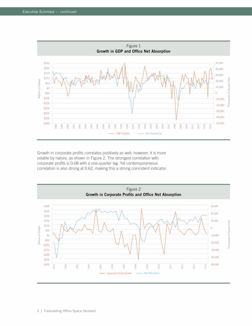
Changes in GDP correlate fairly closely with office net absorption, as shown in Figure 1. The strongest correlation with GDP is 0.54 with a two-quarter lead, indicating that changes in this variable predict changes in office net absorption.

2 | Forecasting Office Space Demand

Figure 1Growth in GDP and Office Net Absorption

1988

1989

199

0

199

1

199

2

199

3

199

4

199

5

1996

199

7

1998

1999

2000

2001

2002

2003

2004

2005

2006

2007

2008

2009

2010

2011

2012

2013

2014

Net AbsorptionGDP Growth

Bill

ions

of D

olla

rs

-$350

-$300

-$250

-$200

-$150

-$100

-$50

$0

$50

$100

$150

$200

$250

-50,000

-40,000

-30,000

-20,000

-10,000

0

10,000

20,000

30,000

40,000

50,000

Thou

sand

s of

Squ

are

Feet

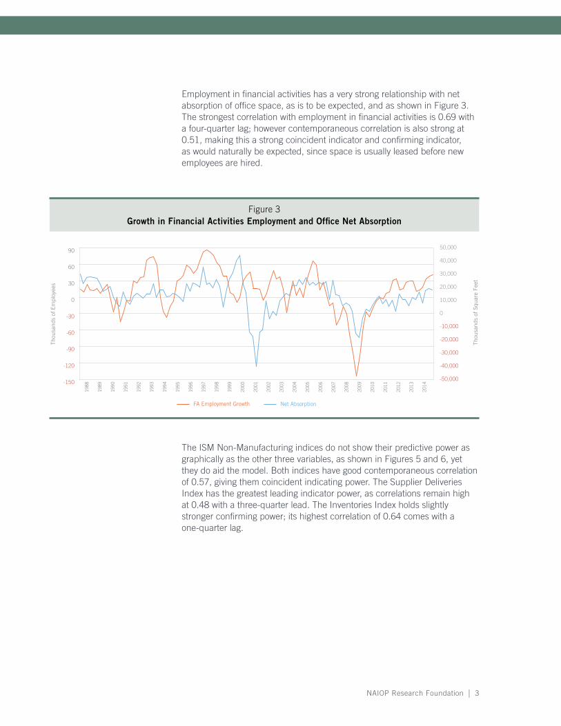
Growth in corporate profits correlates positively as well; however, it is more volatile by nature, as shown in Figure 2. The strongest correlation with corporate profits is 0.68 with a one-quarter lag. Yet contemporaneous correlation is also strong at 0.62, making this a strong coincident indicator.

Figure 2Growth in Corporate Profits and Office Net Absorption

2001

2002

2003

2004

2005

2006

2007

2008

2009

2010

2011

2012

2013

2014-$300

-$250

-$200

-$150

-$100

-$50

$0

$50

$100

$150

$200

$250

$300

-50,000

-40,000

-30,000

-20,000

-10,000

0

10,000

20,000

30,000

Net AbsorptionCorporate Pro�t Growth

Bill

ions

of D

olla

rs

Thou

sand

s of

Squ

are

Feet

Executive Summary — continued


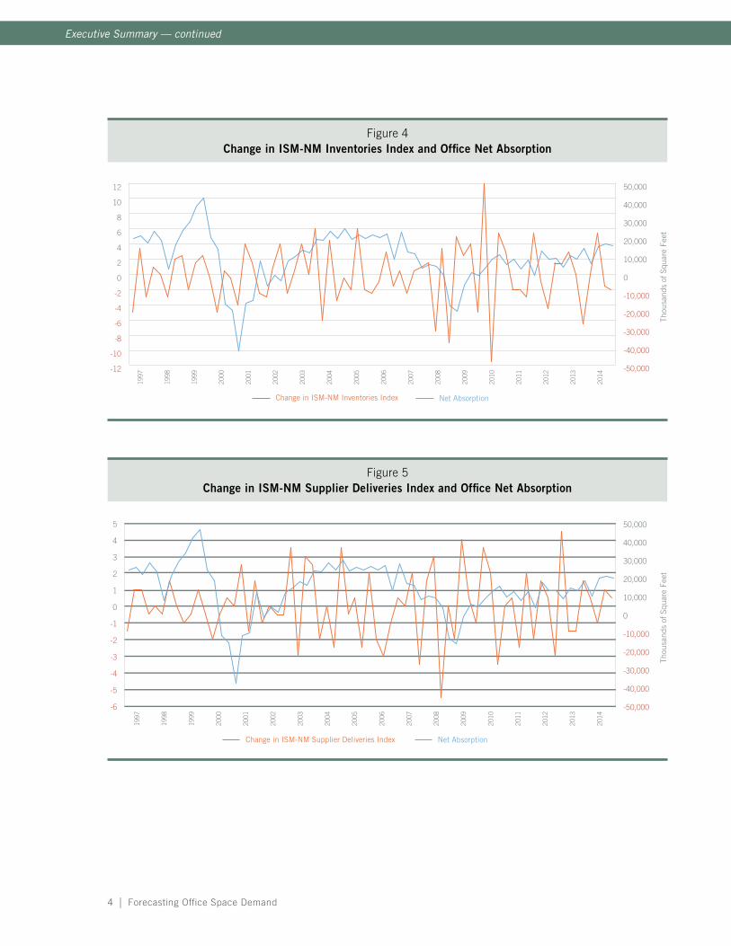
Employment in financial activities has a very strong relationship with net absorption of office space, as is to be expected, and as shown in Figure 3. The strongest correlation with employment in financial activities is 0.69 with a four-quarter lag; however contemporaneous correlation is also strong at 0.51, making this a strong coincident indicator and confirming indicator, as would naturally be expected, since space is usually leased before new employees are hired.

Figure 3Growth in Financial Activities Employment and Office Net Absorption

Thou

sand

s of

Em

ploy

ees

-50,000

-40,000

-30,000

-20,000

-10,000

0

10,000

20,000

30,000

40,000

50,000

-150

-120

-90

-60

-30

0

30

60

90

Thou

sand

s of

Squ

are

Feet

Net AbsorptionFA Employment Growth

1988

1989

199

0

199

1

199

2

199

3

199

4

199

5

1996

199

7

1998

1999

2000

2001

2002

2003

2004

2005

2006

2007

2008

2009

2010

2011

2012

2013

2014

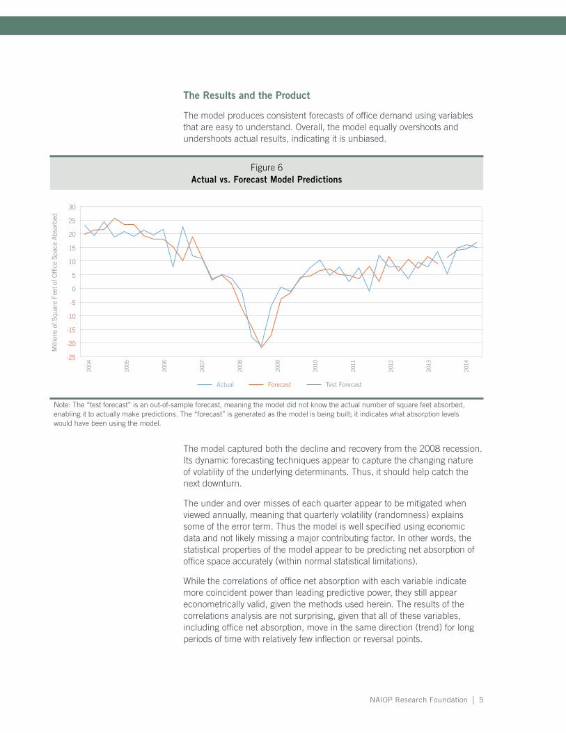
The ISM Non-Manufacturing indices do not show their predictive power as graphically as the other three variables, as shown in Figures 5 and 6, yet they do aid the model. Both indices have good contemporaneous correlation of 0.57, giving them coincident indicating power. The Supplier Deliveries Index has the greatest leading indicator power, as correlations remain high at 0.48 with a three-quarter lead. The Inventories Index holds slightly stronger confirming power; its highest correlation of 0.64 comes with a one-quarter lag.


Executive Summary — continued

Figure 4Change in ISM-NM Inventories Index and Office Net Absorption

-50,000

-40,000

-30,000

-20,000

-10,000

0

10,000

20,000

30,000

40,000

50,000

Thou

sand

s of

Squ

are

Feet

-12

-10

-8

-6

-4

-2

0

2

4

6

8

10

12

199

7

1998

1999

2000

2001

2002

2003

2004

2005

2006

2007

2008

2009

2010

2011

2012

2013

2014

Net AbsorptionChange in ISM-NM Inventories Index

Figure 5Change in ISM-NM Supplier Deliveries Index and Office Net Absorption

-50,000

-40,000

-30,000

-20,000

-10,000

0

10,000

20,000

30,000

40,000

50,000

Thou

sand

s of

Squ

are

Feet

199

7

1998

1999

2000

2001

2002

2003

2004

2005

2006

2007

2008

2009

2010

2011

2012

2013

2014

Net AbsorptionChange in ISM-NM Supplier Deliveries Index

-6

-5

-4

-3

-2

-1

0

1

2

3

4

5


The Results and the Product

The model produces consistent forecasts of office demand using variables that are easy to understand. Overall, the model equally overshoots and undershoots actual results, indicating it is unbiased.

Figure 6Actual vs. Forecast Model Predictions

2004

2005

2006

2007

2008

2009

2010

2011

2012

2013

2014

Actual Forecast

-25

-20

-15

-10

-5

0

5

10

15

20

25

30

Test Forecast

Mill

ions

of S

quar

e Fe

et o

f Of�

ce S

pace

Abs

orbe

d

Note: The “test forecast” is an out-of-sample forecast, meaning the model did not know the actual number of square feet absorbed, enabling it to actually make predictions. The “forecast” is generated as the model is being built; it indicates what absorption levels would have been using the model.

The model captured both the decline and recovery from the 2008 recession. Its dynamic forecasting techniques appear to capture the changing nature of volatility of the underlying determinants. Thus, it should help catch the next downturn.

The under and over misses of each quarter appear to be mitigated when viewed annually, meaning that quarterly volatility (randomness) explains some of the error term. Thus the model is well specified using economic data and not likely missing a major contributing factor. In other words, the statistical properties of the model appear to be predicting net absorption of office space accurately (within normal statistical limitations).

While the correlations of office net absorption with each variable indicate more coincident power than leading predictive power, they still appear econometrically valid, given the methods used herein. The results of the correlations analysis are not surprising, given that all of these variables, including office net absorption, move in the same direction (trend) for long periods of time with relatively few inflection or reversal points.


Introduction

Office space is a critical resource for firms in many industries. For some industries, it represents the only type of real estate they may ever need to occupy. These industries are the so-called “office-using” sectors. The ability to forecast and explain changes in the demand for office space is highly valuable to owners and developers of office buildings. It can help them conduct business planning and make investment decisions. While many unique factors influence how much office space a particular firm will need at a given time, the overall net change in demand — net absorption of office space nationwide — can be explained and thus predicted by macroeconomic variables that are readily observable and known to logically impact the growth of firms in the office-using sectors.

The single most important factor that directly impacts the demand for office space is employment, specifically employment in the office-using sectors. However, in creating models to explain and forecast office space demand, it is not sufficient to simply use measures or forecasts of employment to estimate changes in demand for office space. Why? Because of the way companies actually hire employees and lease office space. Firms must first predict and forecast their own growth (or decline) in demand and profitability, then make decisions to invest and expand (or contract). Once a company decides to expand, it generally acquires productive inputs, including office space, before it actually hires new employees. Thus a predictive model must be able to capture the economic forces that are likely to drive firms to hire and lease space. This study therefore aims to create an accurate model of office space demand, using the most accurate macroeconomic indicators that have historically been related to net changes in demand for office space.


The Process

This office demand study builds upon the methodologies and findings of the NAIOP Research Foundation’s “Industrial Space Demand” white paper (Anderson and Guirguis, 2011) and subsequent biannual forecasts as a starting point to build a model for predicting office space demand. We began by identifying and testing macroeconomic variables with a logical relationship to changes in office space demand. These included variables such as gross domestic product (GDP), total employment, office-using employment, retail sales and corporate profits. Measures of sentiment and activity of the office- using and broader service sectors were investigated as well. Specifically, the Institute for Supply Management’s Non-Manufacturing indices were tested and used in certain model specifications. It is important to note that the ISM indices cannot be future forecasted by the same means as broader macroeconomic variables, such as GDP, and thus cannot always be used to issue long-term forecasts, including those for forecasting office space demand. They do appear useful in the short term, and are included in certain specifications of forecast models of demand for office space.

The primary explanatory variables used in the final model are real GDP, which captures the broadest level of macroeconomic activity and growth; the ISM Non-Manufacturing Inventories and Supplier Deliveries indices, which proxy as a sentiment measure on the future health of office-using firms; corporate profits of domestic industries, which directly captures the financial capacity and growth of firms that may need to expand; and financial activities employment, which is a direct measure and proxy for office-using employment that best fits with changes in office space demand. These measures, along with the lagged measures of net absorption of office space — which serve as the base of the model — make possible an accurate one-year forecast of net absorption of office space nationwide.

Modeling demand for office space has unique challenges and characteristics apart from other forms of real estate forecasting. The largest observable challenge considered ex ante is that intensity of utilization of office space (i.e., square footage leased per employee) varies over time and is subject to change based on firm characteristics, business practices, rental rates and other trends that may or may not directly relate to standard macroeconomic processes. No readily available or reliable means to forecast changes in office space utilization were discovered during this research project. Yet relationships among office space utilization and macroeconomic variables were observed, and showed some statistical linkage. It is important to note that these tests were done to test for robustness and were not used di-rectly in the forecasts of office space demand. The results implied that the changes in macroeconomic variables did capture changes in office space utilization factors, and thus the model controls sufficiently for the amount of occupied square footage per employee. Future research to more directly measure and explain this impact is recommended.


The use of the macroeconomic variables described above appears to be sufficient to control for changes in office space utilization, at least with respect to issuing forecasts as prescribed in this project. Miller, 2013, presents a study and discussion of office utilization trends and points out that corporate goals to reduce office square footage are impacted by companies’ natural need to grow and other economic forces. This study appears to largely agree with Miller’s findings; however, it is not meant to be a direct test of his assertions or findings.

The Process — continued


Data and Methodology

The main explanatory variables utilized in our empirical model are the first lagged of net absorption, the growth rate in real gross domestic product (GDP), ISM Non-Manufacturing Inventories Index (ISM_NM), ISM Non-Manufacturing Supplier Deliveries Index (ISM_NS), Corporate Profits: Domestic Industries (CP), and Financial Activities Employment (FA). Our historical data series for net absorption was obtained from CBRE. The initial model can be stated as follows:

Net Absorption = f(Net Absorptiont-1, GDPt, ISM_NMt, ISM_NSt, CPt, FAt). (1)

Table 1 reports the ordinary least squares (OLS) results from estimating the model for the entire time period from the first quarter of 1991 to the fourth quarter of 2014.

Table 1OLS Regression Result

(Quarterly Data From 1991:01 to 2014:04)

Usable Observations 96

Degrees of Freedom 89

Centered R^2 0.74

R-Bar^2 0.72

Uncentered R^2 0.86

Mean of Dependent Variable 33,794.34

Std Error of Dependent Variable 37,230.40

Standard Error of Estimate 19,552.91

Sum of Squared Residuals 34,026,134,650.00

Regression F(6,89) 42.57

Significance Level of F 0.00

Log Likelihood -1,081.15

Durbin-Watson Statistic 2.04

Variable Coeff Std Error T-Stat Signif

1. Constant 1,258.73 13,253.28 0.09 0.92

2. Net Absorptiont-1 0.38 0.11 3.43 0.00

3. GDP 0.15 0.10 1.50 0.14

4. ISM_NM 13,525.26 4,099.84 3.30 0.00

5. ISM_NS 4,904.26 4,214.98 1.16 0.25

6. CP -25,219.15 11,984.23 -2.10 0.04

7. FA 25,778.86 11,240.61 2.29 0.02


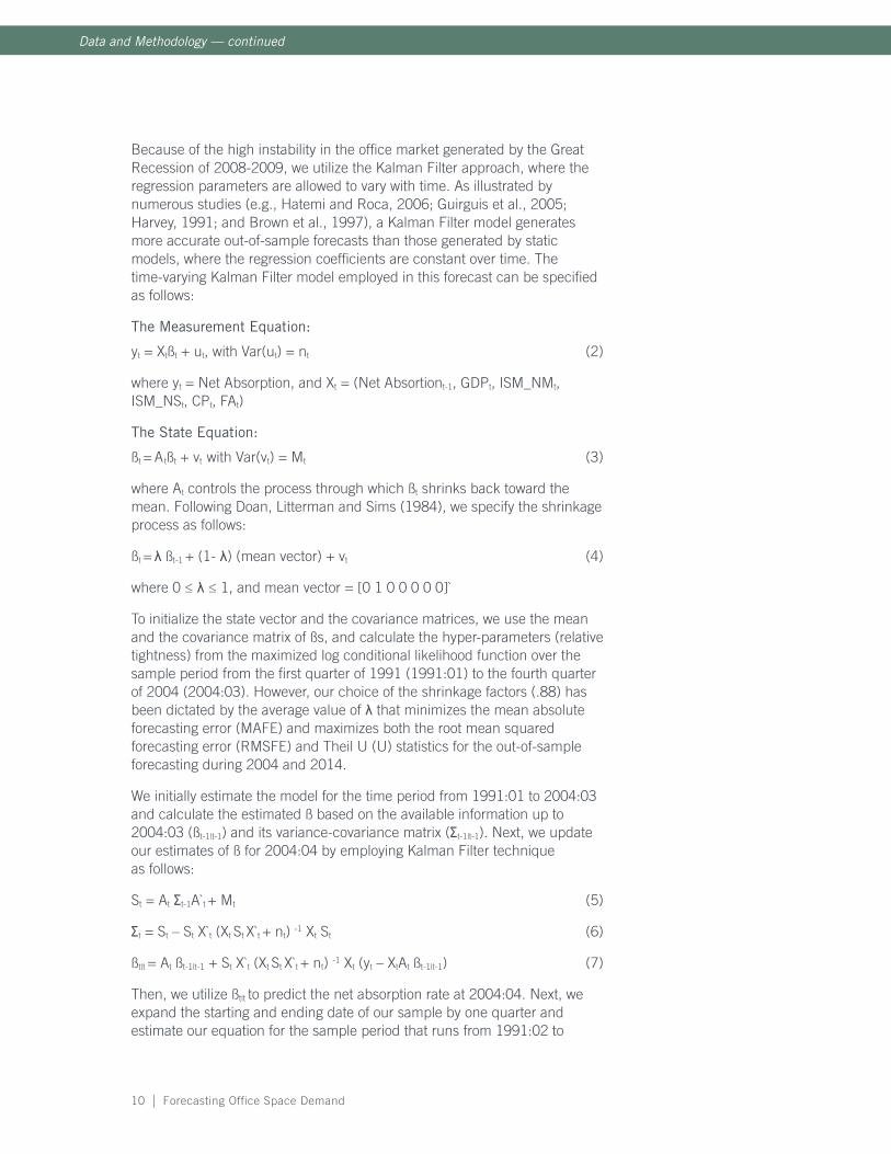
Because of the high instability in the office market generated by the Great Recession of 2008-2009, we utilize the Kalman Filter approach, where the regression parameters are allowed to vary with time. As illustrated by numerous studies (e.g., Hatemi and Roca, 2006; Guirguis et al., 2005; Harvey, 1991; and Brown et al., 1997), a Kalman Filter model generates more accurate out-of-sample forecasts than those generated by static models, where the regression coefficients are constant over time. The time-varying Kalman Filter model employed in this forecast can be specified as follows:

The Measurement Equation:

yt = Xtßt + ut, with Var(ut) = nt (2)

where yt = Net Absorption, and Xt = (Net Absortiont-1, GDPt, ISM_NMt, ISM_NSt, CPt, FAt)

The State Equation:

ßt = Atßt + vt with Var(vt) = Mt (3)

where At controls the process through which ßt shrinks back toward the mean. Following Doan, Litterman and Sims (1984), we specify the shrinkage process as follows:

ßt = λ ßt-1 + (1- λ) (mean vector) + vt (4)

where 0 ≤ λ ≤ 1, and mean vector = [0 1 0 0 0 0 0]`

To initialize the state vector and the covariance matrices, we use the mean and the covariance matrix of ßs, and calculate the hyper-parameters (relative tightness) from the maximized log conditional likelihood function over the sample period from the first quarter of 1991 (1991:01) to the fourth quarter of 2004 (2004:03). However, our choice of the shrinkage factors (.88) has been dictated by the average value of λ that minimizes the mean absolute forecasting error (MAFE) and maximizes both the root mean squared forecasting error (RMSFE) and Theil U (U) statistics for the out-of-sample forecasting during 2004 and 2014.

We initially estimate the model for the time period from 1991:01 to 2004:03 and calculate the estimated ß based on the available information up to 2004:03 (ßt-1|t-1) and its variance-covariance matrix (Σt-1|t-1). Next, we update our estimates of ß for 2004:04 by employing Kalman Filter technique as follows:

St = At Σt-1A`t + Mt (5)

Σt = St – St X`t (Xt St X`t + nt) -1 Xt St (6)

ßt|t = At ßt-1|t-1 + St X`t (Xt St X`t + nt) -1 Xt (yt – XtAt ßt-1|t-1) (7)

Then, we utilize ßt|t to predict the net absorption rate at 2004:04. Next, we expand the starting and ending date of our sample by one quarter and estimate our equation for the sample period that runs from 1991:02 to

Data and Methodology — continued


2004:04, and utilize the estimates to execute Kalman Filter and calculate the one-quarter forecast for 2005:01. We repeat this process until our forecasts cover the sample periods run from 2004:04 to 2013:04. We also calculate the four-quarter forecast from 2014:01 to 2014:04 based on the last estimate of the model on 2013:04.

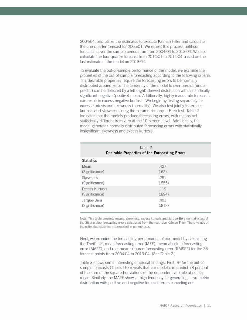
To evaluate the out-of-sample performance of the model, we examine the properties of the out-of-sample forecasting according to the following criteria. The desirable properties require the forecasting errors to be normally distributed around zero. The tendency of the model to over-predict (under- predict) can be detected by a left (right) skewed distribution with a statistically significant negative (positive) mean. Additionally, highly inaccurate forecasts can result in excess negative kurtosis. We begin by testing separately for excess kurtosis and skewness (normality). We also test jointly for excess kurtosis and skewness using the parametric Jarque-Bera test. Table 2 indicates that the models produce forecasting errors, with means not statistically different from zero at the 10 percent level. Additionally, the model generates normally distributed forecasting errors with statistically insignificant skewness and excess kurtosis.

Table 2Desirable Properties of the Forecasting Errors

Statistics

Mean (Significance)

.427(.62)

Skewness(Significance)

.251(.555)

Excess Kurtosis(Significance)

.119(.894)

Jarque-Bera(Significance)

.401(.818)

Note: This table presents means, skewness, excess kurtosis and Jarque-Bera normality test of the 36 one-step forecasting errors calculated from the recursive Kalman Filter. The p-values of the estimated statistics are reported in parentheses.

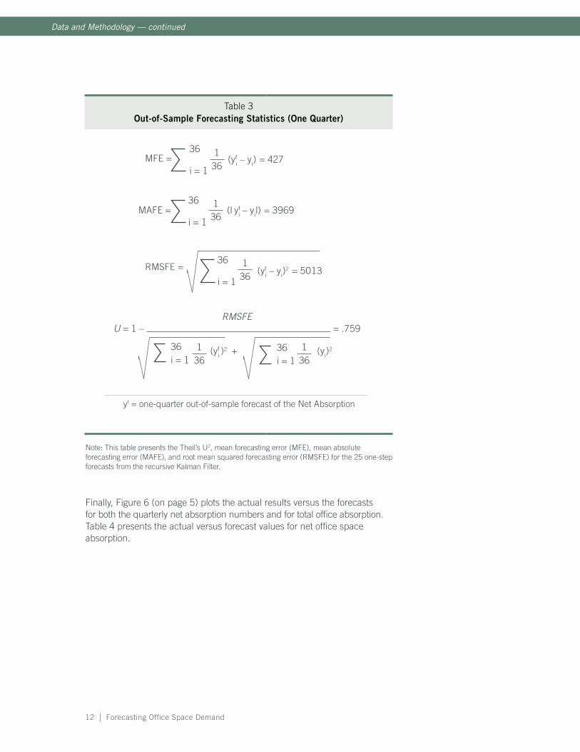
Next, we examine the forecasting performance of our model by calculating the Theil’s U2, mean forecasting error (MFE), mean absolute forecasting error (MAFE), and root mean squared forecasting error (RMSFE) for the 36 forecast points from 2004:04 to 2013:04. (See Table 2.)

Table 3 shows some interesting empirical findings. First, R2 for the out-of-sample forecasts (Theil’s U2) reveals that our model can predict 78 percent of the sum of the squared deviations of the dependent variable about its mean. Similarly, the MAFE shows a high tendency for generating a symmetric distribution with positive and negative forecast errors canceling out.


Table 3Out-of-Sample Forecasting Statistics (One Quarter)

Note: This table presents the Theil’s U2, mean forecasting error (MFE), mean absolute forecasting error (MAFE), and root mean squared forecasting error (RMSFE) for the 25 one-step forecasts from the recursive Kalman Filter.

Finally, Figure 6 (on page 5) plots the actual results versus the forecasts for both the quarterly net absorption numbers and for total office absorption. Table 4 presents the actual versus forecast values for net office space absorption.

MFE =36 i = 1

1 36

(yfi – yi)

= 427

MAFE =1 36

(l yfi – yil)

= 396936 i = 1

RMSFE = (yfi – yi)

2 = 50131 36

36 i = 1

RMSFE U = 1 – = .759

1 36

36 i = 1

(yfi )

2 + 1 36

36 i = 1

(yi)2

yf = one-quarter out-of-sample forecast of the Net Absorption

Data and Methodology — continued


Table 4Actual vs. Forecast Values

(In Thousands of Square Feet)

Date Actual Forecast_1 Forecast_2

2004:04:00 23,461 20,274.04

2005:01:00 19,795 21,605.85

2005:02:00 24,863 21,987.84

2005:03:00 19,180 26,061.05

2005:04:00 21,332 23,645.89

2006:01:00 19,501 23,812.72

2006:02:00 21,635 19,647.73

2006:03:00 19,897 18,488.43

2006:04:00 21,943 18,511.93

2007:01:00 8,232 15,698.63

2007:02:00 23,080 10,619.49

2007:03:00 12,173 19,268.89

2007:04:00 11,262 11,553.378

2008:01:00 3,434 3,818.54

2008:02:00 5,437 5,176.51

2008:03:00 4,225 2,162.58

2008:04:00 -829 -7,156.75

2009:01:00 -17,604 -13,689.12

2009:02:00 -20,456 -21,305.16

2009:03:00 -6,096 -16,809.57

2009:04:00 841 -3,399.69

2010:01:00 -700 -1,333.75

2010:02:00 3,850 4,397.36

2010:03:00 8,003 4,821.86

2010:04:00 10,766 6,893.18

2011:01:00 5,052 7,479.29

2011:02:00 8,124 5,513.14

2011:03:00 2,951 5,283.83

2011:04:00 7,923 4,014.02

2012:01:00 -776 8,444.35

2012:02:00 12,676 2,860.72

2012:03:00 8,164 11,964.40

2012:04:00 8,573 6,815.20

2013:01:00 3,852 11,137.73

2013:02:00 10,019 7,658.73

2013:03:00 8,264 11,944.27

2013:04:00 13,877 9,501.99

2014:01:00 5,602 12,276.54

2014:02:00 15,191 14,817.45

2014:03:00 16,461 15,256.93

2014:04:00 15,430 17,533.20


Conclusion

This research report demonstrates that net absorption of office space can be explained and forecast using macroeconomic variables and measures of firm sentiment. Those who invest in and operate office properties can therefore make better decisions regarding rental rates and lease terms, acquisitions, development, etc. by studying trends in the macro economy. While office-using employment is the most obvious logical determinant of office space demand, this research demonstrates that a more comprehensive set of macroeconomic variables does a better job of explaining and forecasting office leasing activity. This is logical, as a firm’s leasing and expansion decisions typically precede a hiring decision. (In other words, it is difficult for a company to hire people if it does not have enough desks or other adequate office space to accommodate them.)

This model serves as the foundation that we will use to prepare biannual, continually updated forecasts of net absorption of office space for the NAIOP Research Foundation, for use by NAIOP members, other real estate practitioners and the public at large. The methods used herein are dynamic, to account for the changing nature of the underlying macro economy. Further, the exact model specification will adjust dynamically, based on updated future results (i.e., forecasts versus actual results), desired time horizon of forecasts, and innovations in new data and statistical methods.

Overall, it is clear that better investment and new supply decisions can be made using data and thoughtful analysis. Thus, while no forecast is perfect, and shocks and surprises will always occur, it should be the goal of the real estate industry to continually strive to avoid major overbuilding or over-investment by using forecasts such as this as an early warning indicator. Conversely, such forecasts should also be used to confirm and inform future decisions regarding expansion of the office market, i.e., new development.


Works Cited

Anderson, R.I., and H. Guirguis, “Industrial Space Demand,” NAIOP Research Foundation, January 2011.

Brown, J. P., H. Song and A. McGillivray, “Forecasting UK house prices: a time varying coefficient approach,” Economic Modelling, 1997, 14, 529-548.

Doan, T., R. Literman and C.A. Sims, “Forecasting and Conditional Projection Using Realistic Prior Distributions,” Econometric Reviews, 1984, 3, 1-100.

Guirguis, H., C.I. Giannikos and R. Anderson, “The US Housing Market: Asset Pricing Forecasts: Using Time Varying Coefficients,” Journal of Real Estate Finance and Economics, 2005, 30: 33-53.

Harvey, A. “Forecasting, Structural Time Series Models and the Kalman Filter,” Cambridge University Press, Cambridge, 1991.

Hatemi, A., and E. Roca, “Calculating the Optimal Hedge Ratio: Constant, Time Varying and Kalman Filter Approach,” Applied Economics Letters, 2006, 13, 293-299.

Miller, N.G. “Downsizing and Workforce Trends in the Office Market,” Real Estate Issues, 2013, 38, 28-35.

NAIOP RESEARCH FOUNDATION-FUNDED RESEARCH

Available at naioprf.org

Are E-commerce Fulfillment Centers Valued Differently Than Warehouses and Distribution Centers? (2015)

Economic Impacts of Commercial Real Estate, 2015 Edition

Industrial Demand Forecast, Third Quarter 2015

Exploring the New Sharing Economy (2015)

The Promise of E-commerce: Impacts on Retail and Industrial Real Estate (2015)

Selected U.S. Ports Prepare for Panama Canal Expansion (2015)

Preferred Office Locations: Comparing Location Preferences and Performance of Office Space in CBDs, Suburban Vibrant Centers and Suburban Areas (2014)

Economic Impacts of Commercial Real Estate, 2014 Edition

Workplace Innovation Today: The Coworking Center (2014)

Performance and Timing of Secondary Market Activity (2013)

Stabilization of the U.S. Manufacturing Sector and Its Impact on Industrial Space (2013)

The Complexity of Urban Waterfront Development (2012)

The New Borderless Marketplace: Repositioning Retail and Warehouse Properties for Tomorrow (2012)

How Office, Industrial and Retail Development and Construction Contributed to the U.S. Economy in 2011 (2012)

A Development Model for the Middle Ring Suburbs (2012)

How Fuel Costs Affect Logistics Strategies (2011)

Solar Technology Reference Guide (2011)

“The work of the Foundation is absolutely essential to anyone involved in industrial, office, retail and mixed-use development. The Foundation’s

projects are a blueprint for shaping the future and a road map that helps to ensure the success of the developments where we live, work and play.”

Ronald L. Rayevich, Founding Chairman NAIOP Research Foundation

http://www.naioprf.org

We’re Shaping the Future

2201 Cooperative Way, Suite 300 Herndon, VA 20171-3034

703-904-7100 naioprf.org

forecasting office space demand - naiop

Documents