forecasting seasonal time series 1. introduction seasonal time series 1. introduction philip hans...

Forecasting

Seasonal Time Series

1. Introduction

Philip Hans Franses

Econometric Institute

Erasmus University Rotterdam

SMU and NUS, Singapore, April-May 2004

1

Outline of tutorial lectures

1 Introduction

2 Basic models

3 Advanced models

4 Further topics

2

1. Introduction

• How do seasonal time series (in macroeco-

nomics, finance and marketing) look like?

• What do we want to forecast?

• Why is seasonal adjustment often problem-

atic?

3

The contents of this tutorial are largely based

on

• Ghysels and Osborn (2001), The Econo-

metric Analysis of Seasonal Time Series,

Cambridge UP

• Franses and Paap (2004), Periodic Time

Series Models, Oxford UP.

4

These series are the running examples through-

out the lectures:

• Private consumption and GDP for Japan,

quarterly, 1980.1-2001.2 (source: econo-

magic.com)

• M1 for Australia, quarterly, 1975.2-2004.1

(source: economagic.com)

• Total industrial production for the USA,

monthly, 1919.01-2004.02 (source: econo-

magic.com)

• Decile portfolios (based on size), NYSE,

monthly, 1926.08-2002.12 (source: web-

site of Kenneth French) (ranked according

to market capitalization)

• Sales of instant decaf coffee, Netherlands,

weekly, 1994 week 29 to 1998 week 28

5

How do seasonal time series

(in macroeconomics, finance and market-

ing) look like?

Tools:

• Graphs (over time, or per season)

• Autocorrelations (after somehow removingthe trend, usually: ∆1yt = yt − yt−1)

• R2 of regression of ∆1yt on S seasonaldummies or on S (or less) sines and cosines

• Regression of squared residuals from ARmodel for ∆1yt on constant and S−1 sea-sonal dummies (to check for seasonal vari-ation in error variance)

• Autocorrelations per season (to see if thereis periodicity).

Note: these are all just first-stage tools, tosee in what direction one could proceed. Theyshould not be interpreted as final models.

6

40000

60000

80000

100000

120000

140000

160000

80 82 84 86 88 90 92 94 96 98 00

CONSUMPTION INCOME

7

10.6

10.7

10.8

10.9

11.0

11.1

11.2

11.3

80 82 84 86 88 90 92 94 96 98 00

Q1Q2Q3Q4

LC by Season

8

The ”split seasonals” graph for consumption

indicates a rather constant pattern.

The R2 of the ”seasonal dummy regression”

for ∆1yt is 0.927 for log(consumption) and

log(income) it is 0.943.

A suitable model for both log(consumption)

and log(income) turns out to be

∆1yt =4∑

s=1

δsDs,t+ρ1∆1yt−1+εt+θ4εt−4 (1)

The R2 of these models is 0.963 and 0.975, re-

spectively. Hence, constant deterministic sea-

sonality accounts for the majority of trend-free

variation in the data.

9

8000

10000

12000

14000

16000

18000

20000

22000

1980 1985 1990 1995 2000

M1

10

-.06

-.04

-.02

.00

.02

.04

.06

.08

.10

1980 1985 1990 1995 2000

LOG(M1)-LOG(M1(-1))

11

The log of Australian M1 obeys a trend, andsome seasonality, although at first sight notvery regular.

A regression of the growth rates (differencesin logs) on seasonal dummies gives an R2 of0.203.

An AR(5) fits the data for ∆1yt (although theresiduals are not entirely ”white”). The re-gression of the squares of these residuals onan intercept and 3 seasonal dummies gives anF− value of 5.167, hence there is seasonal vari-ation in the variance.

If one fits an AR(2) model for each of theseasons, that is, regress ∆1yt on ∆1yt−1 and∆1yt−2 but allow for different parameters forthe seasons, then the estimation results forquarters 1 to 4 are (0.929, 0.235), (0.226,0.769), (0.070, -0.478), and (0.533, -0.203).This suggests that different models for differ-ent seasons might be useful.

12

0

20

40

60

80

100

120

20 30 40 50 60 70 80 90 00

IPUSA

13

-.16

-.12

-.08

-.04

.00

.04

.08

.12

.16

20 30 40 50 60 70 80 90 00

DY

14

The graphs suggest that the data might be

nonlinear and that there is a break in the vari-

ance, see lecture 4. For now, this is ignored.

A regression of ∆1 of log(production) on S =

12 seasonal dummies gives an R2 of 0.374.

Adding lags at 1, 12 and 13 to this auxiliary

regression model improves the fit to 0.524 (for

1008 data points!), with parameters 0.398, 0.280

and -0.290. There is no residual autocorrela-

tion. The sum of these parameters is 0.388.

Hence, for multi-step ahead forecasts, constant

seasonality dominates. There is also no sea-

sonal heteroskedasticity.

15

The returns (yt) of the 10 decile portfolios

(based on size), NYSE, monthly, 1926.08-2002.12,

can be best described by

yt =12∑

s=1

δsDs,t + εt (2)

εt = ρ1εt−1 + ut (3)

One might expect a ”January effect”, and more

so for the smaller stocks.

The graphs shows the estimates of δs for the

first two and last two deciles. Also the R2

values are higher for lower deciles.

16

-2

0

2

4

6

8

10

1 2 3 4 5 6 7 8 9 10 11 12

DEC1DEC2

DEC9DEC10

17

Comparing the estimated parameters for the

decile models and their associated standard er-

rors suggests that only a few parameters are

significant.

This is even more so in case one has, say,

weekly data, which are common in marketing

and usually coined as store-level data.

One might then consider

yt =52∑

s=1

δsDs,t + εt, (4)

but that involves a large amount of param-

eters. One can then reduce this number by

deleting certain Ds,t variables, but this might

complicate the interpretation.

18

In that case, a more sensible model is

yt = µ +26∑

k=1

[αk cos(2πkt

52) + βk sin(

2πkt

52)] + εt,

(5)

where t = 1,2, .....

A cycle within 52 weeks (an annual cycle) then

corresponds with k = 1, and a cycle within 4

weeks corresponds with k = 13. Other reason-

able cycles would correspond with 2 weeks, 13

weeks and 26 weeks (k = 26, 4 and 2, respec-

tively). Note that sin(2πkt52 ) is equal to 0 for

k = 26, hence the µ.

The next graph shows the fit of this model,

where εt is an AR(1) process, and where only

cycles within 2, 4, 13, 26 and 52 weeks are con-

sidered, and hence there are only 9 variables to

characterize seasonality. The fit is 0.139.

19

7.2

7.6

8.0

8.4

8.8

9.2

25 50 75 100 125 150 175 200

SEASFIT LOG(SALES02)

20

What do we want to forecast?

When one constructs forecasting models fordisaggregated data, one usually want to usethe models for out-of-sample forecasting ofsuch data. Hence, for seasonal data with sea-sonal frequency S, one usually considers fore-casting 1-step ahead, S

2-steps ahead or S-stepsahead.

One may also want to forecast 1 to S stepsahead, that is, say, a year. It is unknownwhether it pays off to use models for disaggre-gated data. Hence, if one wants to forecasta year ahead, it is uncertain whether a modelfor the monthly data does better than a modelfor annual data. Indeed, there are more data,but also more noise and more effort needed tomake a model.

If one aims to forecast a year ahead, one canalso use a model for seasonally adjusted data.(Otherwise : better not!)

21

Why is seasonal adjustment often prob-

lematic?

Seasonal adjustment is usually applied to macroe-

conomic series, in order to make the trend and

the cycle more visible. However, often only

seasonally adjusted data are officially released.

• Seasonally adjusted data are estimated data,

and one should better provide standard er-

rors (Koopman, Franses, OBES 2003)

• Estimated innovations do not concern true

innovations

• Uncertainty about the variable to be fore-

cast: what is it?

• Correlations across variables disturbed

• Why not just take ∆Syt? or ∆1yt after

removal of seasonal dummies?

• Season, trend and cycle can be related.

22

Conclusion for lecture 1

There is substantial seasonal variation in many

economic and business time series.

It seems wise to make a model for the seasonal

data, in order to forecast out of sample, but

also to construct multivariate models.

As we will see in the next lectures: making

models for seasonal data is not that difficult.

23

Forecasting


2. Basic Models

Philip Hans Franses




1


1 Introduction

2 Basic models

3 Advanced models

4 Further topics

2

2. Basic Models

• Constant seasonality (seasonal dummies,

sines and cosines)

• Seasonal random walk

• Airline model

• Basic structural model

3

Constant seasonality

Why could the seasonal pattern be constant?

• Weather: harvests, ice-free lakes and har-

bors, consumption patterns, but also: mood

(think of consumer survey data with sea-

sonality due to less good mood in October

and better mood in January)

• Calendar: festivals, holidays

• Institutions: Tax year, end-of-year bonus,

13-th month salary, children’s holidays

4

A general model for constant seasonality is

yt = µ +

S2∑

k=1

[αk cos(2πkt

S) + βk sin(

2πkt

S)] + ut,

(1)

where t = 1,2, .... and ut is some ARMA type

process.

For example, for S=4, one has

yt = µ+α1 cos(1

2πt)+β1 sin(

1

2πt)+α2 cos(πt)+ut,

(2)

where cos(12πt) is the variable (0,-1,0,1,0,-1,...)

and sin(12πt) is (1,0,-1,0,1,0,...) and cos(πt) is

(-1,1,-1,1,...).

If one considers yt + yt−2, which can be writ-

ten as (1 + L2)yt, then (1 + L2) cos(12πt) = 0

and (1 + L2) sin(12πt) = 0. Moreover, (1 +

L) cos(πt) = 0, and of course, (1− L)µ = 0.

5

This shows that deterministic seasonality can

be removed by applying the transformation (1−L)(1+L)(1+L2) = 1−L4. Note that this also

implies that the error term becomes (1−L4)ut.

Naturally, the relation with the often applied

seasonal dummies regression, that is

yt =4∑

s=1

δsDs,t + ut, (3)

is that µ =∑4

s=1 δs, that α1 = δ4 − δ2, β1 =

δ1 − δ3 and α2 = δ4 − δ3 + δ2 − δ1

6

The constant seasonality model seems appli-

cable to many marketing and tourism series, a

little less so in finance, but it is often not fully

descriptive for macroeconomic series.

Many macroeconomic series display some form

of changing seasonality.

Why could the seasonal pattern be changing?

• Changing consumption patterns (pay for

holidays in advance, eating ice in winter)

• Changing institutions: Tax year, end-of-

year bonus, 13-th month salary, children’s

holidays

• Different responses to exogenous shocks in

different seasons

• Shocks may occur more often in some sea-

sons.

7

Seasonal random walk

A simple model that allows the seasonal pat-tern to change over time is the seasonal ran-dom walk, given by

yt = yt−S + εt. (4)

To understand why seasonality may change,consider the S annual time series Ys,T . Theseasonal random walk implies that for theseannual series it holds that

Ys,T = Ys,T−1 + εs,T . (5)

Hence, each season follows a random walk, anddue to the innovations, the annual series mayintersect, such that ”summer becomes win-ter”.

From graphs it is not easy to discern whethera series is a seasonal random walk or not. Theobservable pattern depends on the starting val-ues of the time series, see the next graph.

8

0

20

40

60

80

100

-40

0

40

80

120

60 65 70 75 80 85 90 95

Y X

Y: starting values all zeroX: starting values 10,-8,14 and -12

9

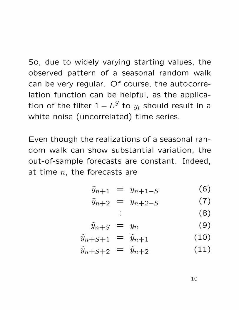
So, due to widely varying starting values, the

observed pattern of a seasonal random walk

can be very regular. Of course, the autocorre-

lation function can be helpful, as the applica-

tion of the filter 1−LS to yt should result in a

white noise (uncorrelated) time series.

Even though the realizations of a seasonal ran-

dom walk can show substantial variation, the

out-of-sample forecasts are constant. Indeed,

at time n, the forecasts are

yn+1 = yn+1−S (6)

yn+2 = yn+2−S (7)

: (8)

yn+S = yn (9)

yn+S+1 = yn+1 (10)

yn+S+2 = yn+2 (11)

10

A subtle form of changing seasonality can also

be described by a time-varying seasonal dummy

parameter model, that is, for S = 4,

yt =4∑

s=1

δs,tDs,t + ut, (12)

where

δs,t = δs,t−S + εs,t. (13)

When the variance of εs,t = 0, then the con-

stant parameter model appears. The amount

of variation depends on the variance of εs,t.

The next slide gives a graphical example (for

simulated data). Canova and Hansen (JBES,

1995) take this model to test for constant sea-

sonality.

11

-30

-20

-10

0

10

20

-20

-10

0

10

20

60 65 70 75 80 85 90 95

Y X

X: constant parametersY: parameter for season 1 is random walk

12

Airline model

An often applied model, popularized by Box

and Jenkins (1970) and named after its appli-

cation to monthly airline passenger data, is the

Airline model, given by

(1−L)(1−LS)yt = (1+θ1L)(1+θSLS)εt. (14)

Note that

(1− L)(1− LS)yt = yt − yt−1 − yt−S + yt−S−1

(15)

It can be proved (Bell, JBES 1987) that as

θS = −1, the model reduces to

(1− L)yt =S∑

s=1

δsDs,t + (1 + θ1L)εt. (16)

13

Strictly speaking, the airline model assumes

S + 1 unit roots. This is due to the fact that

for the characteristic equation

(1− z)(1− zS) = 0 (17)

there are S+1 solutions on the unit circle. For

example, if S = 4 the solutions are (1, 1, -1, i,

-i).

This implies a substantial amount of random

walk like behavior, even though it is corrected

to some extent by the (1 + θ1L)(1 + θSLS)εt

part of the model. In terms of forecasting, it

assumes very wide confidence intervals around

the point forecasts.

Some estimation results for the airline model

are given next.

14

Dependent Variable: LC-LC(-1)-LC(-4)+LC(-5)Method: Least SquaresDate: 04/07/04 Time: 09:48Sample(adjusted): 1981:2 2001:2Included observations: 81 after adjusting endpointsConvergence achieved after 10 iterationsBackcast: 1980:1 1981:1

Variable Coefficient Std. Error t-Statistic Prob.

C -0.000329 0.000264 -1.246930 0.2162MA(1) -0.583998 0.088580 -6.592921 0.0000

SMA(4) -0.591919 0.090172 -6.564320 0.0000

R-squared 0.444787 Mean dependent var -5.01E-05Adjusted R-squared 0.430550 S.D. dependent var 0.016590S.E. of regression 0.012519 Akaike info criterion -5.886745Sum squared resid 0.012225 Schwarz criterion -5.798061Log likelihood 241.4132 F-statistic 31.24325Durbin-Watson stat 2.073346 Prob(F-statistic) 0.000000

Inverted MA Roots .88 .58 .00+.88i -.00 -.88i -.88

15

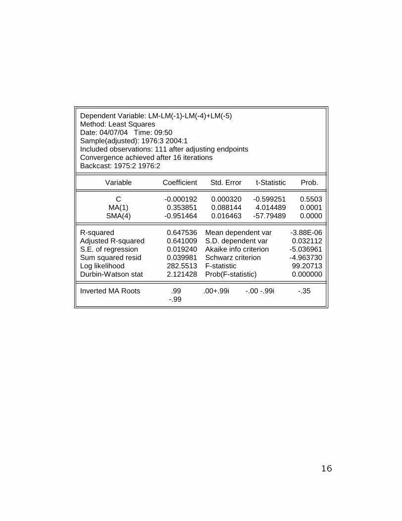
Dependent Variable: LM-LM(-1)-LM(-4)+LM(-5)Method: Least SquaresDate: 04/07/04 Time: 09:50Sample(adjusted): 1976:3 2004:1Included observations: 111 after adjusting endpointsConvergence achieved after 16 iterationsBackcast: 1975:2 1976:2


C -0.000192 0.000320 -0.599251 0.5503MA(1) 0.353851 0.088144 4.014489 0.0001

SMA(4) -0.951464 0.016463 -57.79489 0.0000

R-squared 0.647536 Mean dependent var -3.88E-06Adjusted R-squared 0.641009 S.D. dependent var 0.032112S.E. of regression 0.019240 Akaike info criterion -5.036961Sum squared resid 0.039981 Schwarz criterion -4.963730Log likelihood 282.5513 F-statistic 99.20713Durbin-Watson stat 2.121428 Prob(F-statistic) 0.000000

Inverted MA Roots .99 .00+.99i -.00 -.99i -.35 -.99

16

Dependent Variable: LI-LI(-1)-LI(-12)+LI(-13)Method: Least SquaresDate: 04/07/04 Time: 09:52Sample(adjusted): 1920:02 2004:02Included observations: 1009 after adjusting endpointsConvergence achieved after 11 iterationsBackcast: 1919:01 1920:01


C 2.38E-05 0.000196 0.121473 0.9033MA(1) 0.378388 0.029006 13.04509 0.0000

SMA(12) -0.805799 0.016884 -47.72483 0.0000

R-squared 0.522387 Mean dependent var -0.000108Adjusted R-squared 0.521437 S.D. dependent var 0.031842S.E. of regression 0.022028 Akaike info criterion -4.790041Sum squared resid 0.488142 Schwarz criterion -4.775422Log likelihood 2419.576 F-statistic 550.1535Durbin-Watson stat 1.839223 Prob(F-statistic) 0.000000

Inverted MA Roots .98 .85+.49i .85 -.49i .49+.85i .49 -.85i .00 -.98i -.00+.98i -.38 -.49 -.85i -.49+.85i -.85 -.49i -.85+.49i -.98

17

Basic structural model

A structural time series model for a quarterly

time series can look like

yt = µt + st + wt, wt ∼ NID(0, σ2w) (18)

(1− L)2µt = ut, ut ∼ NID(0, σ2u) (19)

(1 + L + L2 + L3)st = vt, vt ∼ NID(0, σ2v )

(20)

where the error processes wt, ut and vt are also

mutually independent, and where NID denotes

normally and independently distributed.

18

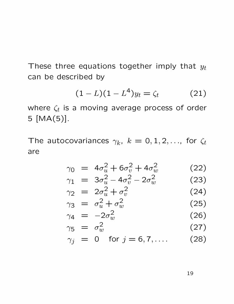
These three equations together imply that yt

can be described by

(1− L)(1− L4)yt = ζt (21)

where ζt is a moving average process of order

5 [MA(5)].

The autocovariances γk, k = 0,1,2, . . ., for ζt

are

γ0 = 4σ2u + 6σ2

v + 4σ2w (22)

γ1 = 3σ2u − 4σ2

v − 2σ2w (23)

γ2 = 2σ2u + σ2

v (24)

γ3 = σ2u + σ2

w (25)

γ4 = −2σ2w (26)

γ5 = σ2w (27)

γj = 0 for j = 6,7, . . . . (28)

19


There are various ways one can describe a time

series (and use that description for forecasting)

with constant or changing seasonal variation.

The next lecture will add even more to this

list.

To make a choice, one needs to test models

against each other. A key distinguishing fea-

ture of the models is the amount of ”random

walk” behavior, or better, the amount of unit

roots (seasonal and non-seasonal). Part of lec-

ture 3 will be devoted to the choice process.

An informal look at graphs and autocorrelation

functions is not sufficient. One needs to make

a decision based on formal tests on parameter

values in auxiliary regressions.

20

Forecasting


3. Advanced Models

Philip Hans Franses




1


1 Introduction

2 Basic models

3 Advanced models

4 Further topics

2

3. Advanced Models

• Seasonal unit roots

• Seasonal cointegration

• Periodic models

• Unit roots in periodic time series

• Periodic cointegration

3

A time series variable has a unit root if the au-

toregressive polynomial (of the autoregressive

model that best describes this variable), con-

tains the component 1 − L, and the moving-

average part does not, where L denotes the

familiar lag operator defined by Lkyt = yt−k,

for k = . . . ,−2,−1,0,1,2, . . . .

For example, the model yt = yt−1 + εt has a

first-order autoregressive polynomial 1−L, as it

can be written as (1−L)yt = εt, and hence data

that can be described by this model, which

is coined the random walk model, are said to

have a unit root. The same holds of course for

the model yt = µ + yt−1 + εt, which is called a

random walk with drift.

4

Solving this last model to the first observation,

that is,

yt = y0 + µt + εt + εt−1 + · · ·+ ε1 (1)

shows that such data display a trend. Due to

the summation of the error terms, it is possible

that data diverge from the overall trend µt for

a long time, and hence at first sight one would

conclude from a graph that there are all kinds

of temporary trends. Therefore, such data are

sometimes said to have a stochastic trend.

The unit roots in seasonal data, which can be

associated with changing seasonality, are the

so-called seasonal unit roots, see Hylleberg et

al (JofE, 1990).

5

For quarterly data, these roots are −1, i, and

−i. For example, data generated from the

model yt = −yt−1 + εt would display season-

ality, but if one were to make graphs with the

split seasonals, then one could observe that the

quarterly data within a year shift places quite

frequently.

Similar observations hold for the model yt =

−yt−2+εt, which can be written as (1+L2)yt =

εt, where the autoregressive polynomial 1+L2

corresponds to the seasonal unit roots i and −i,

as these two values solve the equation 1+z2 =

0. Hence, when a model for yt contains an au-

toregressive polynomial with roots −1 and/or

i, −i, the data are said to have seasonal unit

roots.

6

Testing for seasonal unit roots

The HEGY method for quarterly data amounts

to a regression of ∆4yt on deterministic terms

like an intercept, seasonal dummies, a trend

and seasonal trends on (1 + L + L2 + L3)yt−1,

(−1+ L−L2 + L3)yt−1, −(1+ L2)yt−1, −(1+

L2)yt−2, and on lags of ∆4yt.

The t1-test is for the significance of the pa-

rameter for (1 + L + L2 + L3)yt−1, the t2-test

for (−1 + L − L2 + L3)yt−1 and the joint F34

test for −(1+L2)yt−1 and −(1+L2)yt−2 . An

insignificant test value indicates the presence

of the associated root(s), which are 1, −1, and

the pair i, −i, respectively. Asymptotic theory

for the tests is developed in various studies.

7

The preferable approach is where alternating

dummy variables D1,t−D2,t+D3,t−D4,t, D1,t−D3,t, and D2,t − D4,t are included. Under the

null hypothesis that there is a unit root −1,

the parameter for the first alternating dummy

should also be zero. These joint tests extend

the work of Dickey and Fuller (1981).

When models are created for panels of time se-

ries or for multivariate series, these restrictions

on the deterministics (based on the sine-cosine

notation) are very important.

8

Seasonal cointegration

In case two or more seasonally observed time

series have seasonal unit roots, one may be

interested in testing for common seasonal unit

roots, that is, in testing for seasonal cointegra-

tion. If these series have such roots in com-

mon, they will have common changing sea-

sonal patterns. Engle et al (1993) propose a

method.

Suppose that two time series y1,t and y2,t are

to be differenced using the ∆4 filter. When

y1,t and y2,t have a common non-seasonal unit

root, then the series ut defined by

ut = (1+L+L2+L3)y1,t−α1(1+L+L2+L3)y2,t

(2)

does not need the (1 − L) filter to become

stationary.

9

Seasonal cointegration at the annual frequency

π, corresponding to unit root −1, implies that

vt = (1−L+L2−L3)y1,t−α2(1−L+L2−L3)y2,t

(3)

does not need the (1 + L) differencing filter.

Seasonal cointegration at the annual frequency

π/2, corresponding to the unit roots ±i, means

that

wt = (1− L2)y1,t (4)

− α3(1− L2)y2,t − α4(1− L2)y1,t−1

−α5(1− L2)y2,t−1 (5)

does not have the unit roots ±i.

10

In case all three ut, vt and wt series do not

have the relevant unit roots, the first equation

of a simple version of a seasonal cointegration

model is

∆4y1,t = γ1ut−1+γ2vt−1+γ3wt−2+γ4wt−3+ε1,t,

(6)

where γ1 to γ4 are error correction parameters.

The test method proposed in EGHL is a two-

step method, similar to the Engle-Granger ap-

proach to non-seasonal time series.

11

Seasonal cointegration in a multivariate time

series Yt can also be analyzed using an ex-

tension of the Johansen approach (see Lee

(1992), Johansen and Schaumburg (1999), Kunst

and Franses (OBES 1999). It amounts to test-

ing the ranks of matrices that correspond to

variables which are transformed using the fil-

ters to remove the roots 1, -1 or ± i.

More precise, consider the (m× 1) vector pro-

cess Yt, and assume that it can be described

by the VAR(p) process

Yt = ΘDt + Φ1Yt−1 + · · ·+ ΦpYt−p + et, (7)

where Dt is the (4 × 1) vector process Dt =

(D1,t, D2,t, D3,t, D4,t)′ containing the seasonal

dummies, and where Θ is an (m×4) parameter

matrix.

12

Similar to the Johansen approach and condi-

tional on the assumption that p > 4, the model

can be rewritten as

∆4Yt = ΘDt + Π1Y1,t−1 (8)

+ Π2Y2,t−1 + Π3Y3,t−2 + Π4Y3,t−1 (9)

+ Γ1∆4Yt−1 + · · ·+ Γp−4∆4Yt−(p−4) + et,

where

Y1,t = (1 + L + L2 + L3)Yt

Y2,t = (1− L + L2 − L3)Yt

Y3,t = (1− L2)Yt.

This is a multivariate extension of the univari-

ate HEGY model. The ranks of the matrices

Π1, Π2, Π3 and Π4 determine the number of

cointegration relations at a certain frequency.

13

Periodic models

Consider a univariate time series yt, which is

observed quarterly for N years, that is, t =

1,2, . . . , n. It is assumed that n = 4N . A peri-

odic autoregressive model of order p [PAR(p)]

can be written as

yt = µs + φ1syt−1 + · · ·+ φpsyt−p + εt, (10)

or

φp,s(L)yt = µs + εt (11)

with

φp,s(L) = 1− φ1sL− · · · − φpsLp, (12)

where µs is a seasonally-varying intercept term.

14

The φ1s, . . . , φps are autoregressive parameters

up to order ps which may vary with the season

s, where s = 1,2,3,4. εt is assumed to be

a standard white noise process with constant

variance σ2. This assumption may be relaxed

by allowing εt to have seasonal variance σ2s .

As some φis, i = 1,2, . . . , p, can take zero val-

ues, the order p is the maximum of all ps, where

ps denotes the AR order per season s.

15

Multivariate representation

In general, the PAR(p) process can be rewrit-

ten as an AR(P ) model for the (4 × 1) vec-

tor process YT = (Y1,T , Y2,T , Y3,T , Y4,T )′, T =

1,2, . . . , N , where Ys,T is the observation of yt

in season s of year T , s = 1,2,3,4. The model

is then

Φ0YT = µ+Φ1YT−1+· · ·+ΦPYT−P +εT , (13)

or

Φ(L)YT = µ + εT (14)

with

Φ(L) = Φ0 −Φ1L− · · · −ΦPLP , (15)

16

µ = (µ1, µ2, µ3, µ4)′, εT = (ε1,T , ε2,T , ε3,T , ε4,T )′,

and εs,T is the observation on the error process

εt in season s of year T . Note that the lag op-

erator L applies to data at frequencies t and to

T , that is, Lyt = yt−1 and LYT = YT−1. The

Φ0,Φ1, . . . ,ΦP are 4 × 4 parameter matrices

with elements

Φ0[i, j] =

1 i = j,0 j > i,−φi−j,i i < j,

Φk[i, j] = φi+4k−j,i,

(16)

for i = 1,2,3,4, j = 1,2,3,4, and k = 1,2, . . . , P .

17

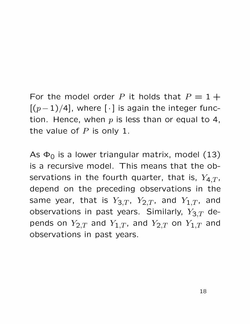
For the model order P it holds that P = 1 +

[(p−1)/4], where [ · ] is again the integer func-

tion. Hence, when p is less than or equal to 4,

the value of P is only 1.

As Φ0 is a lower triangular matrix, model (13)

is a recursive model. This means that the ob-

servations in the fourth quarter, that is, Y4,T ,

depend on the preceding observations in the

same year, that is Y3,T , Y2,T , and Y1,T , and

observations in past years. Similarly, Y3,T de-

pends on Y2,T and Y1,T , and Y2,T on Y1,T and

observations in past years.

18

As an example, consider the PAR(2) process

yt = φ1syt−1 + φ2syt−2 + εt, (17)

which can be written as

Φ0YT = Φ1YT−1 + εT , (18)

with

Φ0 =

1 0 0 0−φ12 1 0 0−φ23 −φ13 1 0

0 −φ24 −φ14 1

and

Φ1 =

0 0 φ21 φ110 0 0 φ220 0 0 00 0 0 0

. (19)

19

A useful representation is based on the pos-

sibility of decomposing a non-periodic AR(p)

polynomial as (1−α1L)(1−α2L) · · · (1−αpL).

Note that this can only be done when the so-

lutions to the characteristic equation for this

AR(p) polynomial are all real-valued. Similar

results hold for the multivariate representation

of a PAR(p) process, and it can be useful to

rewrite (13) as

P∏

i=1

Ξi(L)YT = µ + εT , (20)

where the Ξi(L) are 4 × 4 matrices with ele-

ments which are polynomials in L.

20

A simple example is the PAR(2) process

Ξ1(L)Ξ2(L)YT = εT , (21)

with

Ξ1(L) =

1 0 0 −β1L−β2 1 0 00 −β3 1 00 0 −β4 1

,

Ξ2(L) =

1 0 0 −α1L−α2 1 0 00 −α3 1 00 0 −α4 1

, (22)

21

The PAR(2) can be written as

(1− βsL)(1− αsL)yt = µs + εt. (23)

This expression equals

yt−αsyt−1 = µs+βs(yt−1−αs−1yt−2)+εt, (24)

as, and this is quite important, the lag operator

L also operates on αs, that is, Lαs = αs−1 for

all s = 1,2,3,4 and with α0 = α4.

22

The characteristic equation is

|Ξ1(z)Ξ2(z)| = 0, (25)

which is equivalent to

(1− β1β2β3β4z)(1− α1α2α3α4z) = 0, (26)

and hence the PAR(2) model has one unit root

when either β1β2β3β4 = 1 or α1α2α3α4 = 1,

and has at most two unit roots when both

products equal unity. Obviously, the maximum

number of unity solutions to the characteristic

equation of a PAR(p) process is equal to p.

23

The analogy of a univariate PAR process with

a multivariate time series process can also be

exploited to derive explicit formulae for one-

and multi-step ahead forecasting. It should

be noted that the one-step ahead forecasts

concern one-year ahead forecasts for all four

Ys,T series. For example, for the model YT =

Φ−10 Φ1YT−1+ωT , where ωT = Φ−1

0 εT , the fore-

cast for N + 1 is YN+1 = Φ−10 Φ1YN .

24

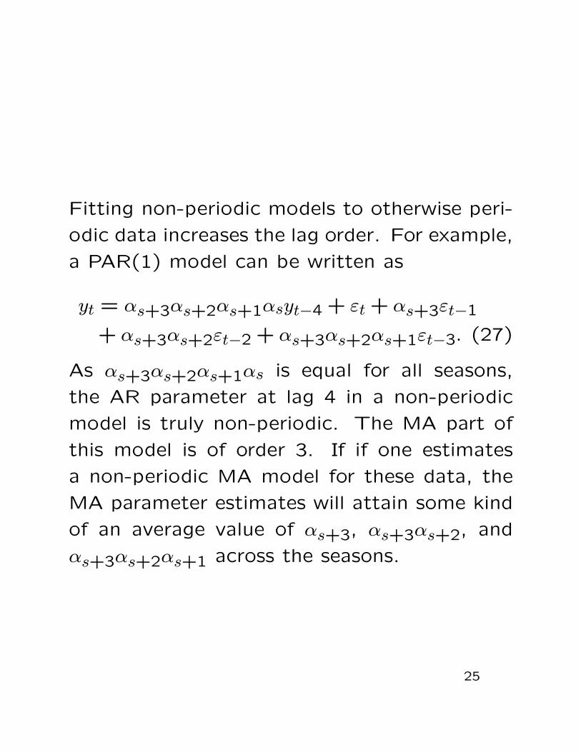
Fitting non-periodic models to otherwise peri-

odic data increases the lag order. For example,

a PAR(1) model can be written as

yt = αs+3αs+2αs+1αsyt−4 + εt + αs+3εt−1

+ αs+3αs+2εt−2 + αs+3αs+2αs+1εt−3. (27)

As αs+3αs+2αs+1αs is equal for all seasons,

the AR parameter at lag 4 in a non-periodic

model is truly non-periodic. The MA part of

this model is of order 3. If if one estimates

a non-periodic MA model for these data, the

MA parameter estimates will attain some kind

of an average value of αs+3, αs+3αs+2, and

αs+3αs+2αs+1 across the seasons.

25

In other words, one might end up considering

an ARMA(4,3) model for PAR(1) data. And,

if one decides not to include an MA part in the

model, one usually needs to increase the order

of the autoregression so as to whiten the er-

rors. This suggests that higher-order AR mod-

els might fit to low-order periodic data. Note

that when αs+3αs+2αs+1αs = 1, this implies a

higher-order AR model for the ∆4 transformed

time series.

Hence, there seems to be a trade-off between

seasonality in parameters and short lags, and

no seasonality in parameters and longer lags.

26

Some further issues:

• Testing for unit roots

• Periodic cointegration

• Forecasting results (Lof, Franses IJF (2002)

analyze periodic and seasonal cointegra-

tion models for bivariate quarterly observed

time series in an empirical forecasting study,

as well as a VAR model in first differences,

with and without cointegration restrictions,

and a VAR model in annual differences.

The VAR model in first differences without

cointegration is best if one-step ahead fore-

casts are considered. For longer forecast

horizons, the VAR model in annual differ-

ences is better. When comparing periodic

versus seasonal cointegration models, the

seasonal cointegration models tend to yield

better forecasts. Finally, there is no clear

indication that multiple equations methods

improve on single equation methods.)

27


Tests for periodic variation in the parameters

and for unit roots allows one to make a choice

between the various models for seasonality.

Models and methods for data with frequencies

higher than 12 can become difficult to use in

practice.

Also, neglected structural breaks can inappro-

priately suggest seasonal unit roots and also

periodicity, see next lecture.

28

Forecasting


4. Further topics

Philip Hans Franses




1


1 Introduction

2 Basic models

3 Advanced models

4 Further topics

2

4. Further topics

• Seasonality in panels of time series

• Nonlinear models for seasonal time series

• Further work

3

Seasonality in panels of time series

Seasonal patterns are quite prominent is manyeconomic data and the search for common sea-sonal patterns can lead to a dramatic reduc-tion in the number of parameters, see Engleand Hylleberg (1996).

Before one can say something about (com-mon) deterministic seasonality, one first has todecide on the number of seasonal unit roots.The basic test regression to test for seasonalunit roots is

Φpi(L)∆4yi,t = µi,t+ρi,1S(L)yi,t−1+ρi,2A(L)yi,t−1

+ ρi,3∆2yi,t−1 + ρi,4∆2yi,t−2 + εt, (1)

where

µi,t = µi + α1,i cos(πt) + α2,i cos(πt

2)

+ α3,i cos(π(t− 1)

2) + δit, (2)

and where ∆k is the k−th order differencingfilter, S(L)yi,t = (1 + L + L2 + L3)yi,t andA(L)yi,t = −(1− L + L2 − L3)yi,t.

4

The model assumes that each series yi,t can

be described by a (pi + 4)−th order autore-

gression. Franses and Kunst (1999) show that

an appropriate test for a seasonal unit root at

the bi-annual frequency is now given by a joint

F−test for ρi,2 and α1,i. An appropriate test

for the two seasonal unit roots at the annual

frequency is then given by a joint F−test for

ρ3,i, ρ4,i, α2,i and α3,i.

Franses and Kunst (1999) consider these F -

tests in a model where the autoregressive pa-

rameters are pooled over the equations. It is

seen that the power of this panel test proce-

dure is rather large.

Additionally, they examine if, once one has

taken care off seasonal unit roots, two or more

series have the same deterministic fluctuations.

This can be done by testing for cross-equation

restrictions.5

Periodic GARCH

Periodic models might also be useful to model

financial time series. They can be used not

only to describe the so-called day-of-the-week

effects, but also to describe the differences in

volatility across the day of the week.

Bollerslev-Ghysels (JBES 1996) propose a pe-

riodic generalized autoregressive conditional het-

eroskedasticity (PGARCH) model.

6

A PAR(p)–PGARCH(1,1) model for a daily ob-

served financial time series yt, t = 1, . . . , n =

5N , can be represented by

xt = yt −5∑

s=1

µs +

p∑

i=1

φisyt−i

Ds,t

=√

htηt

with ηt ∼ N(0,1), (3)

and

ht =5∑

s=1

(ωs + ψsx2t−1)Ds,t + γht−1, (4)

where the xt denotes the residual of the PAR

model for yt, and where Ds,t denote the usual

seasonal dummies but now for the days of the

week, that is, s = 1,2,3,4,5.

7

In order to investigate the properties of the

conditional variance model, it is useful to de-

fine zt = x2t − ht, and to write it as a PARMA

process

x2t =

5∑

s=1

(ωs+(ψs+γ)x2t−1)Ds,t+zt−γzt−1. (5)

This ARMA process for x2t contains time-varying

parameters ψs + γ and hence strictly speaking,

it is not a stationary process.

To investigate the stationarity properties of x2t ,

it is more convenient to write (5) in a param-

eter time-invariant VD representation.

8

Models of seasonality and nonlinearity

A change in the deterministic trend properties

of a time series yt is easily mistaken for the

presence of a unit root.

In a similar vein, if a change in the deter-

ministic seasonal pattern goes undetected, one

might well end up imposing seasonal unit roots,

see Ghysels (JBES, 1994), Smith and Otero

(EL, 1997), Franses, Hoek and Paap (JoE,

1997) and Franses and Vogelsang (RESTAT,

1998)

Changes in deterministic seasonal patterns usu-

ally are modelled by means of one-time abrupt

and discrete changes. However, when sea-

sonal patterns shift due to changes in technol-

ogy, institutions and tastes, for example, these

changes may materialize only gradually.

9

This suggests that a plausible description of

time-varying seasonal patterns is

φ(L)∆1yt =4∑

s=1

δ1,sDs,t(1−G(t; γ, c))

+4∑

s=1

δ2,sDs,tG(t; γ, c) + εt, (6)

where G(t; γ, c) is the logistic function

G(st; γ, c) =1

1 + exp{−γ(st − c)}, γ > 0.

(7)

10

As st increases, the logistic function changes

monotonically from 0 to 1, with the change

being symmetric around the location parame-

ter c, as G(c − z; γ, c) = 1 − G(c + z; γ, c) for

all z. The slope parameter γ determines the

smoothness of the change. As γ → ∞, the

logistic function G(st; γ, c) approaches the in-

dicator function I[st > c], whereas if γ → 0,

G(st; γ, c) → 0.5 for all values of st.

Hence, by taking st = t, the model takes an

“intermediate” position in between determin-

istic seasonality and stochastic trend seasonal-

ity.

11

A nonlinear model with smoothly changing de-

terministic seasonality is

∆1yt = [µ1(1−G(∆4yt−d; γ2, c2))+

µ2G(∆4yt−d; γ2, c2)](1−G(t; γ1, c1))

+ [µ3(1−G(∆4yt−d; γ2, c2))+

µ4G(∆4yt−d; γ2, c2)]G(t; γ1, c1)

+3∑

s=1

δ1,sD∗s,t(1−G(t; γ1, c1))

+3∑

s=1

δ2,sD∗s,tG(t; γ1, c1)

+ (φ1,1∆1yt−1 + · · ·+ φ1,p∆1yt−p)

(1−G(∆4yt−d; γ2, c2))

+ (φ2,1∆1yt−1 + · · ·+ φ2,p∆1yt−p)

G(∆4yt−d; γ2, c2) + εt, (8)

The seasonal pattern is allowed to vary over

time, but it is assumed to be identical in ex-

pansions and recessions at all times.

12

Finally, a time-varying smooth transition model

reads as

∆1yt = ([µ1 +3∑

s=1

δ1,sD∗s,t + φ1,1∆1yt−1

+ · · ·+ φ1,p∆1yt−p](1−G(∆4yt−d; γ2, c2))

+ [µ2 +3∑

s=1

δ2,sD∗s,t + φ2,1∆1yt−1

+· · ·+φ2,p∆1yt−p]G(∆4yt−d; γ2, c2))(1−G(t; γ1, c1))

([µ3 +3∑

s=1

δ3,sD∗s,t + φ3,1∆1yt−1

+ · · ·+ φ3,p∆1yt−p](1−G(∆4yt−d; γ2, c2))

+ [µ4 +3∑

s=1

δ4,sD∗s,t + φ4,1∆1yt−1

+· · ·+φ4,p∆1yt−p]G(∆4yt−d; γ2, c2))G(t; γ1, c1)+εt.

(9)

13

Franses and van Dijk (2004) examine the fore-

casting performance of various models for sea-

sonality and nonlinearity for quarterly industrial

production series of 18 OECD countries. They

find that the accuracy of point forecasts varies

widely across series, across forecast horizons

and across seasons. However, in general, linear

models with fairly simple descriptions of sea-

sonality outperform at short forecast horizons,

whereas nonlinear models with more elaborate

seasonal components dominate at longer hori-

zons. Simpler models are also preferable for in-

terval and density forecasts at short horizons.

Finally, none of the models is found to render

efficient forecasts and hence, forecast combi-

nation is worthwhile.

14


Economic time series (can) have trends, sea-

sonality, nonlinearity, outliers and conditional

volatility.

To fully capture all these features is not an

easy task. Various features may be related.

15

Conclusion for lectures 1-4

Forecasting studies show that model specifi-

cation efforts pay off in terms of performance.

Simple models for seasonally differenced data

forecast well for one or a few steps ahead.

For longer horizons, more involved models are

much better.

Remaining research issues:

• How to achieve parsimony?

• How to date turning points in case trends,

cycles and seasonality are related?

• How to interpret seasonally adjusted data

when trends, cycles and seasonality are re-

lated?

16

Further-reading.bib (April 7, 2004)

References

AT94 . . . . . . . . . . . . . . . . . . . . . . . . . . . . . . . . . . . . . . . . . . . . . . . . . . . . . . . . . . . . . . . . . . . . . . . . . . . . . . . . . . . . . . . . . . . . . . . . . . . . . . . . . . . . . .T. Abeysinghe.Deterministic seasonal models and spurious regressions.Journal of Econometrics, 61:259–272, 1994.

AI94 . . . . . . . . . . . . . . . . . . . . . . . . . . . . . . . . . . . . . . . . . . . . . . . . . . . . . . . . . . . . . . . . . . . . . . . . . . . . . . . . . . . . . . . . . . . . . . . . . . . . . . . . . . . . . .A. Abraham and D. L. Ikenberry.The individual investor and the weekend effect.Journal of Financial and Quantitative Analysis, 29:263–278, 1994.

AG95 . . . . . . . . . . . . . . . . . . . . . . . . . . . . . . . . . . . . . . . . . . . . . . . . . . . . . . . . . . . . . . . . . . . . . . . . . . . . . . . . . . . . . . . . . . . . . . . . . . . . . . . . . . . . . .G. J. Adams and G. C. Goodwin.Parameter estimation for periodic ARMA models.Journal of Time Series Analysis, 16:127–145, 1995.

AA99 . . . . . . . . . . . . . . . . . . . . . . . . . . . . . . . . . . . . . . . . . . . . . . . . . . . . . . . . . . . . . . . . . . . . . . . . . . . . . . . . . . . . . . . . . . . . . . . . . . . . . . . . . . . . . .K. Albertson and J. Aylen.Forecasting using a periodic transfer function: With an application to the UK price of ferrous scrap.International Journal of Forecasting, 15:409–419, 1999.

AJ83 . . . . . . . . . . . . . . . . . . . . . . . . . . . . . . . . . . . . . . . . . . . . . . . . . . . . . . . . . . . . . . . . . . . . . . . . . . . . . . . . . . . . . . . . . . . . . . . . . . . . . . . . . . . . . .J. Andel.Statistical analysis of periodic autoregression.Aplikace Matematiky, 28:364–385, 1983.

AV93 . . . . . . . . . . . . . . . . . . . . . . . . . . . . . . . . . . . . . . . . . . . . . . . . . . . . . . . . . . . . . . . . . . . . . . . . . . . . . . . . . . . . . . . . . . . . . . . . . . . . . . . . . . . . . .P. L. Anderson and A. V. Vecchia.Asymptotic results for periodic autoregressive moving-average models.Journal of Time Series Analysis, 14:1–18, 1993.

BCG01 . . . . . . . . . . . . . . . . . . . . . . . . . . . . . . . . . . . . . . . . . . . . . . . . . . . . . . . . . . . . . . . . . . . . . . . . . . . . . . . . . . . . . . . . . . . . . . . . . . . . . . . . . . . . .C. Bac, J. M. Chevet, and E. Ghysels.Time-series model with periodic stochastic regime switching – Part II: Applications to 16th and 17th centurygrain prices.Macroeconomic Dynamics, 5:32–55, 2001.

BK99 . . . . . . . . . . . . . . . . . . . . . . . . . . . . . . . . . . . . . . . . . . . . . . . . . . . . . . . . . . . . . . . . . . . . . . . . . . . . . . . . . . . . . . . . . . . . . . . . . . . . . . . . . . . . . .K. Balcombe.Seasonal unit root tests with structural breaks in deterministic seasonality.Oxford Bulletin of Economics and Statistics, 61:569–582, 1999.

BM89 . . . . . . . . . . . . . . . . . . . . . . . . . . . . . . . . . . . . . . . . . . . . . . . . . . . . . . . . . . . . . . . . . . . . . . . . . . . . . . . . . . . . . . . . . . . . . . . . . . . . . . . . . . . . . .R. B. Barsky and J. A. Miron.The seasonal cycle and the business cycle.Journal of Political Economy, 97:503–535, 1989.

BL01 . . . . . . . . . . . . . . . . . . . . . . . . . . . . . . . . . . . . . . . . . . . . . . . . . . . . . . . . . . . . . . . . . . . . . . . . . . . . . . . . . . . . . . . . . . . . . . . . . . . . . . . . . . . . . .I. V. Basawa and R. Lund.Large sample properties of parameter estimates for periodic ARMA models.Journal of Time Series Analysis, 22:651–663, 2001.

1


BMM92 . . . . . . . . . . . . . . . . . . . . . . . . . . . . . . . . . . . . . . . . . . . . . . . . . . . . . . . . . . . . . . . . . . . . . . . . . . . . . . . . . . . . . . . . . . . . . . . . . . . . . . . . . . . . .J. J. Beaulieu, J. K. MacKie-Mason, and J. A. Miron.Why do countries and industries with large seasonal cycles also have large business cycles?Quarterly Journal of Economics, 107:621–656, 1992.

BM93 . . . . . . . . . . . . . . . . . . . . . . . . . . . . . . . . . . . . . . . . . . . . . . . . . . . . . . . . . . . . . . . . . . . . . . . . . . . . . . . . . . . . . . . . . . . . . . . . . . . . . . . . . . . . . .J. J. Beaulieu and J. A. Miron.Seasonal unit roots in aggregate U.S. data.Journal of Econometrics, 55:305–328, 1993.

BW87 . . . . . . . . . . . . . . . . . . . . . . . . . . . . . . . . . . . . . . . . . . . . . . . . . . . . . . . . . . . . . . . . . . . . . . . . . . . . . . . . . . . . . . . . . . . . . . . . . . . . . . . . . . . . . .W. R. Bell.A note on overdifferencing and the equivalence of seasonal time series models with monthly means and modelswith (0, 1, 1)12 seasonal parts when θ = 1.Journal of Business and Economic Statistics, 5:383–387, 1987.

BH84 . . . . . . . . . . . . . . . . . . . . . . . . . . . . . . . . . . . . . . . . . . . . . . . . . . . . . . . . . . . . . . . . . . . . . . . . . . . . . . . . . . . . . . . . . . . . . . . . . . . . . . . . . . . . . .W. R. Bell and S. C. Hillmer.Issues involved with the seasonal adjustment of economic time series (with discussion).Journal of Business and Economic Statistics, 2:291–320, 1984.

BH94 . . . . . . . . . . . . . . . . . . . . . . . . . . . . . . . . . . . . . . . . . . . . . . . . . . . . . . . . . . . . . . . . . . . . . . . . . . . . . . . . . . . . . . . . . . . . . . . . . . . . . . . . . . . . . .M. Bentarzi and M. Hallin.On the invertibility of periodic moving-average models.Journal of Time Series Analysis, 15:263–268, 1994.

BH96 . . . . . . . . . . . . . . . . . . . . . . . . . . . . . . . . . . . . . . . . . . . . . . . . . . . . . . . . . . . . . . . . . . . . . . . . . . . . . . . . . . . . . . . . . . . . . . . . . . . . . . . . . . . . . .M. Bentarzi and M. Hallin.Locally optimal tests against periodical autoregression: Parametric and nonparametric approaches.Econometric Theory, 12:88–112, 1996.

BH93 . . . . . . . . . . . . . . . . . . . . . . . . . . . . . . . . . . . . . . . . . . . . . . . . . . . . . . . . . . . . . . . . . . . . . . . . . . . . . . . . . . . . . . . . . . . . . . . . . . . . . . . . . . . . . .H. Bessembinder and M. G. Hertzel.Return autocorrelations around nontrading days.Review of Financial Studies, 6:155–189, 1993.

BBCOS89 . . . . . . . . . . . . . . . . . . . . . . . . . . . . . . . . . . . . . . . . . . . . . . . . . . . . . . . . . . . . . . . . . . . . . . . . . . . . . . . . . . . . . . . . . . . . . . . . . . . . . . . . . .C. R. Birchenhall, R. C. Bladen-Hovell, A. P. L. Chui, D. R. Osborn, and J. P. Smith.A seasonal model of consumption.Economic Journal, 99:837–843, 1989.

BHL94 . . . . . . . . . . . . . . . . . . . . . . . . . . . . . . . . . . . . . . . . . . . . . . . . . . . . . . . . . . . . . . . . . . . . . . . . . . . . . . . . . . . . . . . . . . . . . . . . . . . . . . . . . . . . .P. Bloomfield, H. L. Hurd, and R. B. Lund.Periodic correlation in stratospheric ozone data.Journal of Time Series Analysis, 15:127–150, 1994.

BG96 . . . . . . . . . . . . . . . . . . . . . . . . . . . . . . . . . . . . . . . . . . . . . . . . . . . . . . . . . . . . . . . . . . . . . . . . . . . . . . . . . . . . . . . . . . . . . . . . . . . . . . . . . . . . . .T. Bollerslev and E. Ghysels.Periodic autoregressive conditional heteroscedasticity.Journal of Business and Economic Statistics, 14:139–151, 1996.

BF95 . . . . . . . . . . . . . . . . . . . . . . . . . . . . . . . . . . . . . . . . . . . . . . . . . . . . . . . . . . . . . . . . . . . . . . . . . . . . . . . . . . . . . . . . . . . . . . . . . . . . . . . . . . . . . .H. P. Boswijk and P. H. Franses.Periodic cointegration – representation and inference.Review of Economics and Statistics, 77:436–454, 1995.

2


BF95a . . . . . . . . . . . . . . . . . . . . . . . . . . . . . . . . . . . . . . . . . . . . . . . . . . . . . . . . . . . . . . . . . . . . . . . . . . . . . . . . . . . . . . . . . . . . . . . . . . . . . . . . . . . . .H. P. Boswijk and P. H. Franses.Testing for periodic integration.Economics Letters, 48:241–248, 1995.

BF96 . . . . . . . . . . . . . . . . . . . . . . . . . . . . . . . . . . . . . . . . . . . . . . . . . . . . . . . . . . . . . . . . . . . . . . . . . . . . . . . . . . . . . . . . . . . . . . . . . . . . . . . . . . . . . .H. P. Boswijk and P. H. Franses.Unit roots in periodic autoregressions.Journal of Time Series Analysis, 17:221–245, 1996.

BFH97 . . . . . . . . . . . . . . . . . . . . . . . . . . . . . . . . . . . . . . . . . . . . . . . . . . . . . . . . . . . . . . . . . . . . . . . . . . . . . . . . . . . . . . . . . . . . . . . . . . . . . . . . . . . . .H. P. Boswijk, P. H. Franses, and N. Haldrup.Multiple unit roots in periodic autoregression.Journal of Econometrics, 80:167–193, 1997.

BKP . . . . . . . . . . . . . . . . . . . . . . . . . . . . . . . . . . . . . . . . . . . . . . . . . . . . . . . . . . . . . . . . . . . . . . . . . . . . . . . . . . . . . . . . . . . . . . . . . . . . . . . . . . . . . . .B. L. Bowerman, A. B. Koehler, and D. J. Pack.Forecasting time series with increasing seasonal variation.Journal of Forecasting, 9:419–436, 1990.

BJ70 . . . . . . . . . . . . . . . . . . . . . . . . . . . . . . . . . . . . . . . . . . . . . . . . . . . . . . . . . . . . . . . . . . . . . . . . . . . . . . . . . . . . . . . . . . . . . . . . . . . . . . . . . . . . . .G. E. P. Box and G. M. Jenkins.Time Series Analysis; Forecasting and Control.Holden-Day, San Francisco, 1970.

BE95 . . . . . . . . . . . . . . . . . . . . . . . . . . . . . . . . . . . . . . . . . . . . . . . . . . . . . . . . . . . . . . . . . . . . . . . . . . . . . . . . . . . . . . . . . . . . . . . . . . . . . . . . . . . . . .R. A. Braun and C. L. Evans.Seasonality and equilibrium business cycle theories.Journal of Economic Dynamics and Control, 19:503–532, 1995.

BF97 . . . . . . . . . . . . . . . . . . . . . . . . . . . . . . . . . . . . . . . . . . . . . . . . . . . . . . . . . . . . . . . . . . . . . . . . . . . . . . . . . . . . . . . . . . . . . . . . . . . . . . . . . . . . . .J. Breitung and P. H. Franses.Impulse response functions for periodic integration.Economics Letters, 55:35–40, 1997.

BF98 . . . . . . . . . . . . . . . . . . . . . . . . . . . . . . . . . . . . . . . . . . . . . . . . . . . . . . . . . . . . . . . . . . . . . . . . . . . . . . . . . . . . . . . . . . . . . . . . . . . . . . . . . . . . . .J. Breitung and P. H. Franses.On Phillips–Perron type tests for seasonal unit roots.Econometric Theory, 14:200–221, 1998.

BT01 . . . . . . . . . . . . . . . . . . . . . . . . . . . . . . . . . . . . . . . . . . . . . . . . . . . . . . . . . . . . . . . . . . . . . . . . . . . . . . . . . . . . . . . . . . . . . . . . . . . . . . . . . . . . . .P. Burridge and A. M. R. Taylor.On regression-based tests for seasonal unit roots in the presence of periodic heteroskedasticity.Journal of Econometrics, 104:91–117, 2001.

BW85 . . . . . . . . . . . . . . . . . . . . . . . . . . . . . . . . . . . . . . . . . . . . . . . . . . . . . . . . . . . . . . . . . . . . . . . . . . . . . . . . . . . . . . . . . . . . . . . . . . . . . . . . . . . . . .P. Burridge and K. F. Wallis.Calculating the variance of seasonally adjusted series.Journal of the American Statistical Association, 80:541–552, 1985.

BW90 . . . . . . . . . . . . . . . . . . . . . . . . . . . . . . . . . . . . . . . . . . . . . . . . . . . . . . . . . . . . . . . . . . . . . . . . . . . . . . . . . . . . . . . . . . . . . . . . . . . . . . . . . . . . . .P. Burridge and K. F. Wallis.Seasonal adjustment and Kalman filtering: Extension to periodic variances.Journal of Forecasting, 9:109–118, 1990.

3


CG94 . . . . . . . . . . . . . . . . . . . . . . . . . . . . . . . . . . . . . . . . . . . . . . . . . . . . . . . . . . . . . . . . . . . . . . . . . . . . . . . . . . . . . . . . . . . . . . . . . . . . . . . . . . . . . .F. Canova and E. Ghysels.Changes in seasonal patterns: Are they cyclical?Journal of Economic Dynamics and Control, 18:1143–1171, 1994.

CH95 . . . . . . . . . . . . . . . . . . . . . . . . . . . . . . . . . . . . . . . . . . . . . . . . . . . . . . . . . . . . . . . . . . . . . . . . . . . . . . . . . . . . . . . . . . . . . . . . . . . . . . . . . . . . . .F. Canova and B. E. Hansen.Are seasonal patterns constant over time? A test for seasonal stability.Journal of Business and Economic Statistics, 13:237–252, 1995.

CR92 . . . . . . . . . . . . . . . . . . . . . . . . . . . . . . . . . . . . . . . . . . . . . . . . . . . . . . . . . . . . . . . . . . . . . . . . . . . . . . . . . . . . . . . . . . . . . . . . . . . . . . . . . . . . . .S. Chatterjee and B. Ravikumar.A neoclassical model of seasonal fluctuations.Journal of Monetary Economics, 29:59–86, 1992.

CT85 . . . . . . . . . . . . . . . . . . . . . . . . . . . . . . . . . . . . . . . . . . . . . . . . . . . . . . . . . . . . . . . . . . . . . . . . . . . . . . . . . . . . . . . . . . . . . . . . . . . . . . . . . . . . . .T. Cipra.Periodic moving average processes.Aplikace Matematiky, 30:218–229, 1985.

CT76 . . . . . . . . . . . . . . . . . . . . . . . . . . . . . . . . . . . . . . . . . . . . . . . . . . . . . . . . . . . . . . . . . . . . . . . . . . . . . . . . . . . . . . . . . . . . . . . . . . . . . . . . . . . . . .W. P. Cleveland and G. C. Tiao.Decomposition of seasonal time series: A model for the X-11 program.Journal of the American Statistical Association, 71:581–587, 1976.

CT79 . . . . . . . . . . . . . . . . . . . . . . . . . . . . . . . . . . . . . . . . . . . . . . . . . . . . . . . . . . . . . . . . . . . . . . . . . . . . . . . . . . . . . . . . . . . . . . . . . . . . . . . . . . . . . .W. P. Cleveland and G. C. Tiao.Modelling seasonal time series.Revue Economique Appliquee, 32:107–129, 1979.

D04 . . . . . . . . . . . . . . . . . . . . . . . . . . . . . . . . . . . . . . . . . . . . . . . . . . . . . . . . . . . . . . . . . . . . . . . . . . . . . . . . . . . . . . . . . . . . . . . . . . . . . . . . . . . . . . .O. Darne.Seasonal cointegration for monthly data.Economics Letters, 82:349–356, 2004.

DL94 . . . . . . . . . . . . . . . . . . . . . . . . . . . . . . . . . . . . . . . . . . . . . . . . . . . . . . . . . . . . . . . . . . . . . . . . . . . . . . . . . . . . . . . . . . . . . . . . . . . . . . . . . . . . . .H. Dezhbakhsh and D. Levy.Periodic properties of interpolated time series.Economics Letters, 44:221–228, 1994.

DHF84 . . . . . . . . . . . . . . . . . . . . . . . . . . . . . . . . . . . . . . . . . . . . . . . . . . . . . . . . . . . . . . . . . . . . . . . . . . . . . . . . . . . . . . . . . . . . . . . . . . . . . . . . . . . . .D. A. Dickey, D. P. Hasza, and W. A. Fuller.Testing for unit roots in seasonal time series.Journal of the American Statistical Association, 79:355–367, 1984.

EGH89 . . . . . . . . . . . . . . . . . . . . . . . . . . . . . . . . . . . . . . . . . . . . . . . . . . . . . . . . . . . . . . . . . . . . . . . . . . . . . . . . . . . . . . . . . . . . . . . . . . . . . . . . . . . . .R. F. Engle, C. W. J. Granger, and J. J. Hallman.Merging short- and long-run forecasts: An application of seasonal cointegration to monthly electricity salesforecasting.Journal of Econometrics, 40:45–62, 1989.

EGHL93 . . . . . . . . . . . . . . . . . . . . . . . . . . . . . . . . . . . . . . . . . . . . . . . . . . . . . . . . . . . . . . . . . . . . . . . . . . . . . . . . . . . . . . . . . . . . . . . . . . . . . . . . . . . .R. F. Engle, C. W. J. Granger, S. Hylleberg, and H. S. Lee.Seasonal cointegration: The Japanese consumption function.Journal of Econometrics, 55:275–298, 1993.

4


FM89 . . . . . . . . . . . . . . . . . . . . . . . . . . . . . . . . . . . . . . . . . . . . . . . . . . . . . . . . . . . . . . . . . . . . . . . . . . . . . . . . . . . . . . . . . . . . . . . . . . . . . . . . . . . . . .M. Faig.Seasonal fluctuations and the demand for money.Quarterly Journal of Economics, 99:847–861, 1989.

FV90 . . . . . . . . . . . . . . . . . . . . . . . . . . . . . . . . . . . . . . . . . . . . . . . . . . . . . . . . . . . . . . . . . . . . . . . . . . . . . . . . . . . . . . . . . . . . . . . . . . . . . . . . . . . . . .D. F. Foster and S. Viswanathan.A theory of the interday variations in volume, variance, and trading costs in security markets.Review of Financial Studies, 3:593–624, 1990.

FP91 . . . . . . . . . . . . . . . . . . . . . . . . . . . . . . . . . . . . . . . . . . . . . . . . . . . . . . . . . . . . . . . . . . . . . . . . . . . . . . . . . . . . . . . . . . . . . . . . . . . . . . . . . . . . . .P. H. Franses.Model Selection and Seasonality in Time Series.PhD thesis, Tinbergen Institute, Amsterdam, 1991.

FP91c . . . . . . . . . . . . . . . . . . . . . . . . . . . . . . . . . . . . . . . . . . . . . . . . . . . . . . . . . . . . . . . . . . . . . . . . . . . . . . . . . . . . . . . . . . . . . . . . . . . . . . . . . . . . .P. H. Franses.A multivariate approach to modeling univariate seasonal time series.Econometric Institute Report 9101, Erasmus University Rotterdam, 1991.

FP91b . . . . . . . . . . . . . . . . . . . . . . . . . . . . . . . . . . . . . . . . . . . . . . . . . . . . . . . . . . . . . . . . . . . . . . . . . . . . . . . . . . . . . . . . . . . . . . . . . . . . . . . . . . . . .P. H. Franses.Seasonality, nonstationarity and the forecasting of monthly time series.International Journal of Forecasting, 7:199–208, 1991.

FP93 . . . . . . . . . . . . . . . . . . . . . . . . . . . . . . . . . . . . . . . . . . . . . . . . . . . . . . . . . . . . . . . . . . . . . . . . . . . . . . . . . . . . . . . . . . . . . . . . . . . . . . . . . . . . . .P. H. Franses.Periodically integrated subset autoregressions for Dutch industrial production and money stock.Journal of Forecasting, 12:601–613, 1993.

FP94 . . . . . . . . . . . . . . . . . . . . . . . . . . . . . . . . . . . . . . . . . . . . . . . . . . . . . . . . . . . . . . . . . . . . . . . . . . . . . . . . . . . . . . . . . . . . . . . . . . . . . . . . . . . . . .P. H. Franses.A multivariate approach to modeling univariate seasonal time series.Journal of Econometrics, 63:133–151, 1994.

FP95b . . . . . . . . . . . . . . . . . . . . . . . . . . . . . . . . . . . . . . . . . . . . . . . . . . . . . . . . . . . . . . . . . . . . . . . . . . . . . . . . . . . . . . . . . . . . . . . . . . . . . . . . . . . . .P. H. Franses.A vector of quarters representation for bivariate time series.Econometric Reviews, 14:55–63, 1995.

FP95c . . . . . . . . . . . . . . . . . . . . . . . . . . . . . . . . . . . . . . . . . . . . . . . . . . . . . . . . . . . . . . . . . . . . . . . . . . . . . . . . . . . . . . . . . . . . . . . . . . . . . . . . . . . . .P. H. Franses.The effects of seasonally adjusting a periodic autoregressive process.Computational Statistics and Data Analysis, 19:683–704, 1995.

FP95a . . . . . . . . . . . . . . . . . . . . . . . . . . . . . . . . . . . . . . . . . . . . . . . . . . . . . . . . . . . . . . . . . . . . . . . . . . . . . . . . . . . . . . . . . . . . . . . . . . . . . . . . . . . . .P. H. Franses.On periodic autoregressions and structural breaks in seasonal time series.Environmetrics, 6:451–456, 1995.

FP96b . . . . . . . . . . . . . . . . . . . . . . . . . . . . . . . . . . . . . . . . . . . . . . . . . . . . . . . . . . . . . . . . . . . . . . . . . . . . . . . . . . . . . . . . . . . . . . . . . . . . . . . . . . . . .P. H. Franses.Multi-step forecast error variances for periodically integrated time series.Journal of Forecasting, 15:83–95, 1996.

5


FP96 . . . . . . . . . . . . . . . . . . . . . . . . . . . . . . . . . . . . . . . . . . . . . . . . . . . . . . . . . . . . . . . . . . . . . . . . . . . . . . . . . . . . . . . . . . . . . . . . . . . . . . . . . . . . . .P. H. Franses.Periodicity and Stochastic Trends in Economic Time Series.Oxford University Press, Oxford, 1996.

FP98 . . . . . . . . . . . . . . . . . . . . . . . . . . . . . . . . . . . . . . . . . . . . . . . . . . . . . . . . . . . . . . . . . . . . . . . . . . . . . . . . . . . . . . . . . . . . . . . . . . . . . . . . . . . . . .P. H. Franses.Time Series Models for Business and Economic Forecasting.Cambridge University Press, Cambridge, 1998.

FH97 . . . . . . . . . . . . . . . . . . . . . . . . . . . . . . . . . . . . . . . . . . . . . . . . . . . . . . . . . . . . . . . . . . . . . . . . . . . . . . . . . . . . . . . . . . . . . . . . . . . . . . . . . . . . . .P. H. Franses and B. Hobijn.Critical values for unit root tests in seasonal time series.Journal of Applied Statistics, 24:28–48, 1997.

FHP97 . . . . . . . . . . . . . . . . . . . . . . . . . . . . . . . . . . . . . . . . . . . . . . . . . . . . . . . . . . . . . . . . . . . . . . . . . . . . . . . . . . . . . . . . . . . . . . . . . . . . . . . . . . . . .P. H. Franses, H. Hoek, and R. Paap.Bayesian analysis of seasonal unit roots and seasonal mean shifts.Journal of Econometrics, 78:359–380, 1997.

FHL95 . . . . . . . . . . . . . . . . . . . . . . . . . . . . . . . . . . . . . . . . . . . . . . . . . . . . . . . . . . . . . . . . . . . . . . . . . . . . . . . . . . . . . . . . . . . . . . . . . . . . . . . . . . . . .P. H. Franses, S. Hylleberg, and H. S. Lee.Spurious deterministic seasonality.Economics Letters, 48:249–256, 1995.

FK95 . . . . . . . . . . . . . . . . . . . . . . . . . . . . . . . . . . . . . . . . . . . . . . . . . . . . . . . . . . . . . . . . . . . . . . . . . . . . . . . . . . . . . . . . . . . . . . . . . . . . . . . . . . . . . .P. H. Franses and T. Kloek.A periodic cointegration model of quarterly consumption.Applied Stochastic Models and Data Analysis, 11:159–166, 1995.

FK98 . . . . . . . . . . . . . . . . . . . . . . . . . . . . . . . . . . . . . . . . . . . . . . . . . . . . . . . . . . . . . . . . . . . . . . . . . . . . . . . . . . . . . . . . . . . . . . . . . . . . . . . . . . . . . .P. H. Franses and A. B. Koehler.A model selection strategy for time series with increasing seasonal variation.International Journal of Forecasting, 14:405–414, 1998.

FK97 . . . . . . . . . . . . . . . . . . . . . . . . . . . . . . . . . . . . . . . . . . . . . . . . . . . . . . . . . . . . . . . . . . . . . . . . . . . . . . . . . . . . . . . . . . . . . . . . . . . . . . . . . . . . . .P. H. Franses and G. Koop.A Bayesian analysis of periodic integration.Journal of Forecasting, 16:509–532, 1997.

FK99 . . . . . . . . . . . . . . . . . . . . . . . . . . . . . . . . . . . . . . . . . . . . . . . . . . . . . . . . . . . . . . . . . . . . . . . . . . . . . . . . . . . . . . . . . . . . . . . . . . . . . . . . . . . . . .P. H. Franses and R. M. Kunst.On the role of seasonal intercepts in seasonal cointegration.Oxford Bulletin of Economics and Statistics, 61:409–433, 1999.

FM97 . . . . . . . . . . . . . . . . . . . . . . . . . . . . . . . . . . . . . . . . . . . . . . . . . . . . . . . . . . . . . . . . . . . . . . . . . . . . . . . . . . . . . . . . . . . . . . . . . . . . . . . . . . . . . .P. H. Franses and M. McAleer.Testing nested and non-nested periodically integrated autoregressive models.Communications in Statistics – Theory and Methods, 26:1461–1475, 1997.

FM97b . . . . . . . . . . . . . . . . . . . . . . . . . . . . . . . . . . . . . . . . . . . . . . . . . . . . . . . . . . . . . . . . . . . . . . . . . . . . . . . . . . . . . . . . . . . . . . . . . . . . . . . . . . . . .P. H. Franses and M. McAleer.Testing periodically integrated autoregressive models.Mathematics and Computers in Simulation, 43:457–455, 1997.

6


FO97 . . . . . . . . . . . . . . . . . . . . . . . . . . . . . . . . . . . . . . . . . . . . . . . . . . . . . . . . . . . . . . . . . . . . . . . . . . . . . . . . . . . . . . . . . . . . . . . . . . . . . . . . . . . . . .P. H. Franses and M. Ooms.A periodic long-memory model for quarterly UK inflation.International Journal of Forecasting, 13:117–126, 1997.

FPP94 . . . . . . . . . . . . . . . . . . . . . . . . . . . . . . . . . . . . . . . . . . . . . . . . . . . . . . . . . . . . . . . . . . . . . . . . . . . . . . . . . . . . . . . . . . . . . . . . . . . . . . . . . . . . .P. H. Franses and R. Paap.Model selection in periodic autoregressions.Oxford Bulletin of Economics and Statistics, 56:421–440, 1994.

FPP95 . . . . . . . . . . . . . . . . . . . . . . . . . . . . . . . . . . . . . . . . . . . . . . . . . . . . . . . . . . . . . . . . . . . . . . . . . . . . . . . . . . . . . . . . . . . . . . . . . . . . . . . . . . . . .P. H. Franses and R. Paap.Seasonality and stochastic trends in German consumption and income 1960.1-1987.4.Empirical Economics, 20:109–132, 1995.

FPP96 . . . . . . . . . . . . . . . . . . . . . . . . . . . . . . . . . . . . . . . . . . . . . . . . . . . . . . . . . . . . . . . . . . . . . . . . . . . . . . . . . . . . . . . . . . . . . . . . . . . . . . . . . . . . .P. H. Franses and R. Paap.Periodic integration: Further results on model selection and forecasting.Statistical Papers, 37:33–52, 1996.

FPP00 . . . . . . . . . . . . . . . . . . . . . . . . . . . . . . . . . . . . . . . . . . . . . . . . . . . . . . . . . . . . . . . . . . . . . . . . . . . . . . . . . . . . . . . . . . . . . . . . . . . . . . . . . . . . .P. H. Franses and R. Paap.Modelling day-of-the-week seasonality in the S&P 500 index.Applied Financial Economics, 10:483–488, 2000.

FP02 . . . . . . . . . . . . . . . . . . . . . . . . . . . . . . . . . . . . . . . . . . . . . . . . . . . . . . . . . . . . . . . . . . . . . . . . . . . . . . . . . . . . . . . . . . . . . . . . . . . . . . . . . . . . . .P. H. Franses and R. Paap.Forecasting with periodic autoregressive time series models.In M. P. Clements and D. F. Hendry, editors, A Companion to Economic Forecasting, chapter 19, pages 432–452.Basil Blackwell, Oxford, 2002.

FR93 . . . . . . . . . . . . . . . . . . . . . . . . . . . . . . . . . . . . . . . . . . . . . . . . . . . . . . . . . . . . . . . . . . . . . . . . . . . . . . . . . . . . . . . . . . . . . . . . . . . . . . . . . . . . . .P. H. Franses and G. Romijn.Periodic integration in quarterly UK macroeconomic variables.International Journal of Forecasting, 9:467–476, 1993.

FT00 . . . . . . . . . . . . . . . . . . . . . . . . . . . . . . . . . . . . . . . . . . . . . . . . . . . . . . . . . . . . . . . . . . . . . . . . . . . . . . . . . . . . . . . . . . . . . . . . . . . . . . . . . . . . . .P. H. Franses and A. M. R. Taylor.Determining the order of differencing in seasonal time series processes.Econometrics Journal, 3:250–264, 2000.

FV98 . . . . . . . . . . . . . . . . . . . . . . . . . . . . . . . . . . . . . . . . . . . . . . . . . . . . . . . . . . . . . . . . . . . . . . . . . . . . . . . . . . . . . . . . . . . . . . . . . . . . . . . . . . . . . .P. H. Franses and T. J. Vogelsang.On seasonal cycles, unit roots and mean shifts.Review of Economics and Statistics, 80:231–240, 1998.

FK80 . . . . . . . . . . . . . . . . . . . . . . . . . . . . . . . . . . . . . . . . . . . . . . . . . . . . . . . . . . . . . . . . . . . . . . . . . . . . . . . . . . . . . . . . . . . . . . . . . . . . . . . . . . . . . .K. R. French.Stock returns and the weekend effect.Journal of Financial Economics, 8:55–69, 1980.

FR86 . . . . . . . . . . . . . . . . . . . . . . . . . . . . . . . . . . . . . . . . . . . . . . . . . . . . . . . . . . . . . . . . . . . . . . . . . . . . . . . . . . . . . . . . . . . . . . . . . . . . . . . . . . . . . .K. R. French and R. Roll.Stock return variances: The arrival of information and the reaction of traders.Journal of Financial Economics, 17:5–26, 1986.

7


GM78 . . . . . . . . . . . . . . . . . . . . . . . . . . . . . . . . . . . . . . . . . . . . . . . . . . . . . . . . . . . . . . . . . . . . . . . . . . . . . . . . . . . . . . . . . . . . . . . . . . . . . . . . . . . . . .M. Gersovitz and J. G. MacKinnon.Seasonality in regression: An application of smoothness priors.Journal of the American Statistical Association, 73:264–273, 1978.

GE88 . . . . . . . . . . . . . . . . . . . . . . . . . . . . . . . . . . . . . . . . . . . . . . . . . . . . . . . . . . . . . . . . . . . . . . . . . . . . . . . . . . . . . . . . . . . . . . . . . . . . . . . . . . . . . .E. Ghysels.A study towards a dynamic theory of seasonality for economic time series.Journal of the American Statistical Association, 83:168–172, 1988.

GE90 . . . . . . . . . . . . . . . . . . . . . . . . . . . . . . . . . . . . . . . . . . . . . . . . . . . . . . . . . . . . . . . . . . . . . . . . . . . . . . . . . . . . . . . . . . . . . . . . . . . . . . . . . . . . . .E. Ghysels.Unit root tests and the statistical pitfalls of seasonal adjustment: The case of US postwar real gross nationalproduct.Journal of Business and Economic Statistics, 8:145–152, 1990.

GE93 . . . . . . . . . . . . . . . . . . . . . . . . . . . . . . . . . . . . . . . . . . . . . . . . . . . . . . . . . . . . . . . . . . . . . . . . . . . . . . . . . . . . . . . . . . . . . . . . . . . . . . . . . . . . . .E. Ghysels.On scoring asymmetric periodic probability models of turning point forecasts.Journal of Forecasting, 12:227–238, 1993.

GE94 . . . . . . . . . . . . . . . . . . . . . . . . . . . . . . . . . . . . . . . . . . . . . . . . . . . . . . . . . . . . . . . . . . . . . . . . . . . . . . . . . . . . . . . . . . . . . . . . . . . . . . . . . . . . . .E. Ghysels.On the periodic structure of the business cycle.Journal of Business and Economic Statistics, 12:289–298, 1994.

GE00 . . . . . . . . . . . . . . . . . . . . . . . . . . . . . . . . . . . . . . . . . . . . . . . . . . . . . . . . . . . . . . . . . . . . . . . . . . . . . . . . . . . . . . . . . . . . . . . . . . . . . . . . . . . . . .E. Ghysels.Time-series model with periodic stochastic regime switching – part I: Theory.Macroeconomic Dynamics, 4:467–486, 2000.

GGS96 . . . . . . . . . . . . . . . . . . . . . . . . . . . . . . . . . . . . . . . . . . . . . . . . . . . . . . . . . . . . . . . . . . . . . . . . . . . . . . . . . . . . . . . . . . . . . . . . . . . . . . . . . . . . .E. Ghysels, C. W. J. Granger, and P. L. Siklos.Is seasonal adjustment a linear or nonlinear data filtering process?Journal of Business and Economic Statistics, 14:374–386, 1996.

GHL96 . . . . . . . . . . . . . . . . . . . . . . . . . . . . . . . . . . . . . . . . . . . . . . . . . . . . . . . . . . . . . . . . . . . . . . . . . . . . . . . . . . . . . . . . . . . . . . . . . . . . . . . . . . . . .E. Ghysels, A. Hall, and H. S. Lee.On periodic structures and testing for seasonal unit roots.Journal of the American Statistical Association, 91:1551–1559, 1996.

GLN94 . . . . . . . . . . . . . . . . . . . . . . . . . . . . . . . . . . . . . . . . . . . . . . . . . . . . . . . . . . . . . . . . . . . . . . . . . . . . . . . . . . . . . . . . . . . . . . . . . . . . . . . . . . . . .E. Ghysels, H. S. Lee, and J. Noh.Testing for unit roots in seasonal time series: Some theoretical extensions and a Monte Carlo investigation.Journal of Econometrics, 62:415–442, 1994.

GMT98 . . . . . . . . . . . . . . . . . . . . . . . . . . . . . . . . . . . . . . . . . . . . . . . . . . . . . . . . . . . . . . . . . . . . . . . . . . . . . . . . . . . . . . . . . . . . . . . . . . . . . . . . . . . . .E. Ghysels, R. E. McCulloch, and R. S. Tsay.Bayesian inference for periodic regime-switching models.Journal of Applied Econometrics, 13:129–144, 1998.

GO01 . . . . . . . . . . . . . . . . . . . . . . . . . . . . . . . . . . . . . . . . . . . . . . . . . . . . . . . . . . . . . . . . . . . . . . . . . . . . . . . . . . . . . . . . . . . . . . . . . . . . . . . . . . . . . .E. Ghysels and D. R. Osborn.The Econometric Analysis of Seasonal Time Series.Cambridge University Press, Cambridge, 2001.

8


GP93 . . . . . . . . . . . . . . . . . . . . . . . . . . . . . . . . . . . . . . . . . . . . . . . . . . . . . . . . . . . . . . . . . . . . . . . . . . . . . . . . . . . . . . . . . . . . . . . . . . . . . . . . . . . . . .E. Ghysels and P. Perron.The effect of seasonal adjustment filters on tests for a unit root.Journal of Econometrics, 55:57–98, 1993.

GE61 . . . . . . . . . . . . . . . . . . . . . . . . . . . . . . . . . . . . . . . . . . . . . . . . . . . . . . . . . . . . . . . . . . . . . . . . . . . . . . . . . . . . . . . . . . . . . . . . . . . . . . . . . . . . . .E. G. Gladyshev.Periodically correlated random sequences.Soviet Mathematics, 2:385–388, 1961.

GN70 . . . . . . . . . . . . . . . . . . . . . . . . . . . . . . . . . . . . . . . . . . . . . . . . . . . . . . . . . . . . . . . . . . . . . . . . . . . . . . . . . . . . . . . . . . . . . . . . . . . . . . . . . . . . . .D. M. Grether and M. Nerlove.Some properties of optimal seasonal adjustment.Econometrica, 38:682–703, 1970.

HS93 . . . . . . . . . . . . . . . . . . . . . . . . . . . . . . . . . . . . . . . . . . . . . . . . . . . . . . . . . . . . . . . . . . . . . . . . . . . . . . . . . . . . . . . . . . . . . . . . . . . . . . . . . . . . . .L. P. Hansen and T. J. Sargent.Seasonality and approximation errors in rational expectations models.Journal of Econometrics, 55:21–56, 1993.

HA89 . . . . . . . . . . . . . . . . . . . . . . . . . . . . . . . . . . . . . . . . . . . . . . . . . . . . . . . . . . . . . . . . . . . . . . . . . . . . . . . . . . . . . . . . . . . . . . . . . . . . . . . . . . . . . .A. C. Harvey.Forecasting, Structural Time Series Models and the Kalman Filter.Cambridge University Press, Cambridge, 1989.

HF82 . . . . . . . . . . . . . . . . . . . . . . . . . . . . . . . . . . . . . . . . . . . . . . . . . . . . . . . . . . . . . . . . . . . . . . . . . . . . . . . . . . . . . . . . . . . . . . . . . . . . . . . . . . . . . .D. P. Hasza and W. A. Fuller.Testing for nonstationary parameter specifications in seasonal time series models.Annals of Statistics, 10:1209–1216, 1982.

HH97 . . . . . . . . . . . . . . . . . . . . . . . . . . . . . . . . . . . . . . . . . . . . . . . . . . . . . . . . . . . . . . . . . . . . . . . . . . . . . . . . . . . . . . . . . . . . . . . . . . . . . . . . . . . . . .H. Herwartz.Performance of periodic error correction models in forecasting consumption data.International Journal of Forecasting, 13:421–431, 1997.

HT82 . . . . . . . . . . . . . . . . . . . . . . . . . . . . . . . . . . . . . . . . . . . . . . . . . . . . . . . . . . . . . . . . . . . . . . . . . . . . . . . . . . . . . . . . . . . . . . . . . . . . . . . . . . . . . .S. C. Hillmer and G. C. Tiao.An ARIMA-model-based approach to seasonal adjustment.Journal of the American Statistical Association, 77:63–70, 1982.

HG91 . . . . . . . . . . . . . . . . . . . . . . . . . . . . . . . . . . . . . . . . . . . . . . . . . . . . . . . . . . . . . . . . . . . . . . . . . . . . . . . . . . . . . . . . . . . . . . . . . . . . . . . . . . . . . .H. L. Hurd and N. L. Gerr.Graphical methods for determining the presence of periodic correlation.Journal of Time Series Analysis, 12:337–350, 1991.

HS86 . . . . . . . . . . . . . . . . . . . . . . . . . . . . . . . . . . . . . . . . . . . . . . . . . . . . . . . . . . . . . . . . . . . . . . . . . . . . . . . . . . . . . . . . . . . . . . . . . . . . . . . . . . . . . .S. Hylleberg.Seasonality in Regression.Academic Press, Orlando, 1986.

HS92 . . . . . . . . . . . . . . . . . . . . . . . . . . . . . . . . . . . . . . . . . . . . . . . . . . . . . . . . . . . . . . . . . . . . . . . . . . . . . . . . . . . . . . . . . . . . . . . . . . . . . . . . . . . . . .S. Hylleberg.Modelling Seasonality.Oxford University Press, Oxford, 1992.

9


HS94 . . . . . . . . . . . . . . . . . . . . . . . . . . . . . . . . . . . . . . . . . . . . . . . . . . . . . . . . . . . . . . . . . . . . . . . . . . . . . . . . . . . . . . . . . . . . . . . . . . . . . . . . . . . . . .S. Hylleberg.Modelling seasonal variation.In C.P. Hargreaves, editor, Nonstationary Time Series Analysis and Cointegration. Oxford University Press,Oxford, 1994.

HS95 . . . . . . . . . . . . . . . . . . . . . . . . . . . . . . . . . . . . . . . . . . . . . . . . . . . . . . . . . . . . . . . . . . . . . . . . . . . . . . . . . . . . . . . . . . . . . . . . . . . . . . . . . . . . . .S. Hylleberg.Tests for seasonal unit roots: General to specific or specific to general?Journal of Econometrics, 69:5–25, 1995.

HEGY90 . . . . . . . . . . . . . . . . . . . . . . . . . . . . . . . . . . . . . . . . . . . . . . . . . . . . . . . . . . . . . . . . . . . . . . . . . . . . . . . . . . . . . . . . . . . . . . . . . . . . . . . . . . . .S. Hylleberg, R. F. Engle, C. W. J. Granger, and B. S. Yoo.Seasonal integration and cointegration.Journal of Econometrics, 44:215–238, 1990.

HJS93 . . . . . . . . . . . . . . . . . . . . . . . . . . . . . . . . . . . . . . . . . . . . . . . . . . . . . . . . . . . . . . . . . . . . . . . . . . . . . . . . . . . . . . . . . . . . . . . . . . . . . . . . . . . . .S. Hylleberg, C. Jørgensen, and N. K. Sørensen.Seasonality in macroeconomic time series.Empirical Economics, 18:321–335, 1993.

JT00 . . . . . . . . . . . . . . . . . . . . . . . . . . . . . . . . . . . . . . . . . . . . . . . . . . . . . . . . . . . . . . . . . . . . . . . . . . . . . . . . . . . . . . . . . . . . . . . . . . . . . . . . . . . . . .T. Jaditz.Seasonality in variance is common in macro time series.Journal of Business, 73:245–254, 2000.

JK90 . . . . . . . . . . . . . . . . . . . . . . . . . . . . . . . . . . . . . . . . . . . . . . . . . . . . . . . . . . . . . . . . . . . . . . . . . . . . . . . . . . . . . . . . . . . . . . . . . . . . . . . . . . . . . .A. Jaeger and R. M. Kunst.Seasonal adjustment and measuring persistence in output.Journal of Applied Econometrics, 5:47–58, 1990.

JS99 . . . . . . . . . . . . . . . . . . . . . . . . . . . . . . . . . . . . . . . . . . . . . . . . . . . . . . . . . . . . . . . . . . . . . . . . . . . . . . . . . . . . . . . . . . . . . . . . . . . . . . . . . . . . . .S. Johansen and E. Shaumburg.Likelihood analysis of seasonal cointegration.Journal of Econometrics, 88:301–339, 1999.

JB67 . . . . . . . . . . . . . . . . . . . . . . . . . . . . . . . . . . . . . . . . . . . . . . . . . . . . . . . . . . . . . . . . . . . . . . . . . . . . . . . . . . . . . . . . . . . . . . . . . . . . . . . . . . . . . .R. H. Jones and W. M. Brelsford.Time series with periodic structure.Biometrika, 54:403–407, 1967.

KS84 . . . . . . . . . . . . . . . . . . . . . . . . . . . . . . . . . . . . . . . . . . . . . . . . . . . . . . . . . . . . . . . . . . . . . . . . . . . . . . . . . . . . . . . . . . . . . . . . . . . . . . . . . . . . . .D. B. Keim and R.F. Stambaugh.A further investigation of the weekend effect in stock returns.Journal of Finance, 39:819–835, 1984.

KF99 . . . . . . . . . . . . . . . . . . . . . . . . . . . . . . . . . . . . . . . . . . . . . . . . . . . . . . . . . . . . . . . . . . . . . . . . . . . . . . . . . . . . . . . . . . . . . . . . . . . . . . . . . . . . . .F. Kleibergen and P. H. Franses.Cointegration in a periodic vector autoregression.Econometric Institute Report 9906/A, Erasmus University Rotterdam, 1999.

KF02 . . . . . . . . . . . . . . . . . . . . . . . . . . . . . . . . . . . . . . . . . . . . . . . . . . . . . . . . . . . . . . . . . . . . . . . . . . . . . . . . . . . . . . . . . . . . . . . . . . . . . . . . . . . . . .S. J. Koopman and P. H. Franses.Constructing seasonally adjusted data with time-varying confidence intervals.Oxford Bulletin of Economics and Statistics, 64:509–526, 2002.

10


KS93 . . . . . . . . . . . . . . . . . . . . . . . . . . . . . . . . . . . . . . . . . . . . . . . . . . . . . . . . . . . . . . . . . . . . . . . . . . . . . . . . . . . . . . . . . . . . . . . . . . . . . . . . . . . . . .S.D. Krane.Induced seasonality and production-smoothing models of inventory behavior.Journal of Econometrics, 55:135–168, 1993.

KR93 . . . . . . . . . . . . . . . . . . . . . . . . . . . . . . . . . . . . . . . . . . . . . . . . . . . . . . . . . . . . . . . . . . . . . . . . . . . . . . . . . . . . . . . . . . . . . . . . . . . . . . . . . . . . . .R. M. Kunst.Seasonal cointegration in macroeconomic systems: Case studies for small and large european countries.Review of Economics and Statistics, 75:325–330, 1993.

KR97 . . . . . . . . . . . . . . . . . . . . . . . . . . . . . . . . . . . . . . . . . . . . . . . . . . . . . . . . . . . . . . . . . . . . . . . . . . . . . . . . . . . . . . . . . . . . . . . . . . . . . . . . . . . . . .R. M. Kunst.Testing for cyclical non-stationarity in autoregressive processes.Journal of Time Series Analysis, 18:123–135, 1997.

KE02 . . . . . . . . . . . . . . . . . . . . . . . . . . . . . . . . . . . . . . . . . . . . . . . . . . . . . . . . . . . . . . . . . . . . . . . . . . . . . . . . . . . . . . . . . . . . . . . . . . . . . . . . . . . . . .E. Kurozumi.Testing for periodic stationarity.Econometric Reviews, 21:243–270, 2002.

LG77 . . . . . . . . . . . . . . . . . . . . . . . . . . . . . . . . . . . . . . . . . . . . . . . . . . . . . . . . . . . . . . . . . . . . . . . . . . . . . . . . . . . . . . . . . . . . . . . . . . . . . . . . . . . . . .G Laroque.Analyse d’une methode de desaissonnalisation: Le programme X-11 du bureau of Census, version trimestrielle.Annales de l’INSEE, 28:105–127, 1977.

LH92 . . . . . . . . . . . . . . . . . . . . . . . . . . . . . . . . . . . . . . . . . . . . . . . . . . . . . . . . . . . . . . . . . . . . . . . . . . . . . . . . . . . . . . . . . . . . . . . . . . . . . . . . . . . . . .H. S. Lee.Maximum likelihood inference on cointegration and seasonal cointegration.Journal of Econometrics, 54:351–365, 1992.

LS97 . . . . . . . . . . . . . . . . . . . . . . . . . . . . . . . . . . . . . . . . . . . . . . . . . . . . . . . . . . . . . . . . . . . . . . . . . . . . . . . . . . . . . . . . . . . . . . . . . . . . . . . . . . . . . .H. S Lee and P. L. Siklos.The role of seasonality in economic time series: Reinterpreting money-output causality in U.S. data.International Journal of Forecasting, 13:381–392, 1997.

LR02 . . . . . . . . . . . . . . . . . . . . . . . . . . . . . . . . . . . . . . . . . . . . . . . . . . . . . . . . . . . . . . . . . . . . . . . . . . . . . . . . . . . . . . . . . . . . . . . . . . . . . . . . . . . . . .P. A. W. Lewis and B. K. Ray.Nonlinear modelling of periodic threshold autoregressions using TSMARS.Journal of Time Series Analysis, 23:459–471, 2002.

LF01 . . . . . . . . . . . . . . . . . . . . . . . . . . . . . . . . . . . . . . . . . . . . . . . . . . . . . . . . . . . . . . . . . . . . . . . . . . . . . . . . . . . . . . . . . . . . . . . . . . . . . . . . . . . . . .M. Lof and P. H. Franses.On forecasting cointegrated seasonal time series.International Journal of Forecasting, 17:607–621, 2001.

MA85 . . . . . . . . . . . . . . . . . . . . . . . . . . . . . . . . . . . . . . . . . . . . . . . . . . . . . . . . . . . . . . . . . . . . . . . . . . . . . . . . . . . . . . . . . . . . . . . . . . . . . . . . . . . . . .A. Maravall.On structural time series models and the characterization of components.Journal of Business and Economic Statistics, 3:350–355, 1985.

MP87 . . . . . . . . . . . . . . . . . . . . . . . . . . . . . . . . . . . . . . . . . . . . . . . . . . . . . . . . . . . . . . . . . . . . . . . . . . . . . . . . . . . . . . . . . . . . . . . . . . . . . . . . . . . . . .A. Maravall and D. A. Pierce.A prototypical seasonal adjustment model.Journal of Time Series Analysis, 8:177–193, 1987.

11


MA93 . . . . . . . . . . . . . . . . . . . . . . . . . . . . . . . . . . . . . . . . . . . . . . . . . . . . . . . . . . . . . . . . . . . . . . . . . . . . . . . . . . . . . . . . . . . . . . . . . . . . . . . . . . . . . .A. I. McLeod.Parsimony, model adequacy and periodic correlation in time series forecasting.International Statistical Review, 61:387–393, 1993.

MA94 . . . . . . . . . . . . . . . . . . . . . . . . . . . . . . . . . . . . . . . . . . . . . . . . . . . . . . . . . . . . . . . . . . . . . . . . . . . . . . . . . . . . . . . . . . . . . . . . . . . . . . . . . . . . . .A. I. McLeod.Diagnostic checking of periodic autoregression models with application.Journal of Time Series Analysis, 15:221–233, 1994.

MJ86 . . . . . . . . . . . . . . . . . . . . . . . . . . . . . . . . . . . . . . . . . . . . . . . . . . . . . . . . . . . . . . . . . . . . . . . . . . . . . . . . . . . . . . . . . . . . . . . . . . . . . . . . . . . . . .J. A. Miron.Seasonal fluctuations and the life cycle-permanent income model of consumption.Journal of Political Economy, 94:1258–1279, 1986.

MJ94 . . . . . . . . . . . . . . . . . . . . . . . . . . . . . . . . . . . . . . . . . . . . . . . . . . . . . . . . . . . . . . . . . . . . . . . . . . . . . . . . . . . . . . . . . . . . . . . . . . . . . . . . . . . . . .J. A. Miron.The economics of seasonal cycles.In C.A. Sims, editor, Advances in Econometrics, Sixth World Congress of the Econometric Society. CambridgeUniversity Press, Cambridge UK, 1994.

MZ88 . . . . . . . . . . . . . . . . . . . . . . . . . . . . . . . . . . . . . . . . . . . . . . . . . . . . . . . . . . . . . . . . . . . . . . . . . . . . . . . . . . . . . . . . . . . . . . . . . . . . . . . . . . . . . .J. A. Miron and S. P. Zeldes.Seasonality, cost shocks, and the production smoothing model of inventories.Econometrica, 56:877–908, 1988.

NMH85 . . . . . . . . . . . . . . . . . . . . . . . . . . . . . . . . . . . . . . . . . . . . . . . . . . . . . . . . . . . . . . . . . . . . . . . . . . . . . . . . . . . . . . . . . . . . . . . . . . . . . . . . . . . . .D. J. Noakes, A. I. McLeod, and K. W. Hipel.Forecasting monthly riverflow time series.International Journal of Forecasting, 1:179–190, 1985.

OF97 . . . . . . . . . . . . . . . . . . . . . . . . . . . . . . . . . . . . . . . . . . . . . . . . . . . . . . . . . . . . . . . . . . . . . . . . . . . . . . . . . . . . . . . . . . . . . . . . . . . . . . . . . . . . . .M. Ooms and P. H. Franses.On periodic correlations between estimated seasonal and nonseasonal components in German and US unem-ployment.Journal of Business and Economic Statistics, 15:470–481, 1997.

OF01 . . . . . . . . . . . . . . . . . . . . . . . . . . . . . . . . . . . . . . . . . . . . . . . . . . . . . . . . . . . . . . . . . . . . . . . . . . . . . . . . . . . . . . . . . . . . . . . . . . . . . . . . . . . . . .M. Ooms and P. H. Franses.A seasonal periodic long memory model for monthly river flows.Environmental Modelling and Sofware, 16:559–569, 2001.

OD88 . . . . . . . . . . . . . . . . . . . . . . . . . . . . . . . . . . . . . . . . . . . . . . . . . . . . . . . . . . . . . . . . . . . . . . . . . . . . . . . . . . . . . . . . . . . . . . . . . . . . . . . . . . . . . .D. R. Osborn.Seasonality and habit persistence in a life-cycle model of consumption.Journal of Applied Econometrics, 3:255–266, 1988.

OD90 . . . . . . . . . . . . . . . . . . . . . . . . . . . . . . . . . . . . . . . . . . . . . . . . . . . . . . . . . . . . . . . . . . . . . . . . . . . . . . . . . . . . . . . . . . . . . . . . . . . . . . . . . . . . . .D. R. Osborn.A survey of seasonality in UK macroeconomic variables.International Journal of Forecasting, 6:327–336, 1990.

12


OD91 . . . . . . . . . . . . . . . . . . . . . . . . . . . . . . . . . . . . . . . . . . . . . . . . . . . . . . . . . . . . . . . . . . . . . . . . . . . . . . . . . . . . . . . . . . . . . . . . . . . . . . . . . . . . . .D. R. Osborn.The implications of periodically varying coefficients for seasonal time-series processes.Journal of Econometrics, 48:373–384, 1991.

OD93 . . . . . . . . . . . . . . . . . . . . . . . . . . . . . . . . . . . . . . . . . . . . . . . . . . . . . . . . . . . . . . . . . . . . . . . . . . . . . . . . . . . . . . . . . . . . . . . . . . . . . . . . . . . . . .D. R. Osborn.Comment on engle et al. [1993].Journal of Econometrics, 55:299–303, 1993.

OD00 . . . . . . . . . . . . . . . . . . . . . . . . . . . . . . . . . . . . . . . . . . . . . . . . . . . . . . . . . . . . . . . . . . . . . . . . . . . . . . . . . . . . . . . . . . . . . . . . . . . . . . . . . . . . . .D. R. Osborn.Cointegration for seasonal time series processes.unpublised working paper, University of Manchester, 2000.

OCSB88 . . . . . . . . . . . . . . . . . . . . . . . . . . . . . . . . . . . . . . . . . . . . . . . . . . . . . . . . . . . . . . . . . . . . . . . . . . . . . . . . . . . . . . . . . . . . . . . . . . . . . . . . . . . .D. R. Osborn, A. P. L. Chui, J. P. Smith, and C. R. Birchenhall.Seasonality and the order of integration for consumption.Oxford Bulletin of Economics and Statistics, 50:361–377, 1988.

OR02 . . . . . . . . . . . . . . . . . . . . . . . . . . . . . . . . . . . . . . . . . . . . . . . . . . . . . . . . . . . . . . . . . . . . . . . . . . . . . . . . . . . . . . . . . . . . . . . . . . . . . . . . . . . . . .D. R. Osborn and P. M. M. Rodrigues.Asymptotic distributions of seasonal unit root tests: A unifying approach.Econometric Reviews, 21:221–241, 2002.

OS89 . . . . . . . . . . . . . . . . . . . . . . . . . . . . . . . . . . . . . . . . . . . . . . . . . . . . . . . . . . . . . . . . . . . . . . . . . . . . . . . . . . . . . . . . . . . . . . . . . . . . . . . . . . . . . .D. R. Osborn and J. P. Smith.The performance of periodic autoregressive models in forecasting seasonal U.K. consumption.Journal of Business and Economic Statistics, 7:117–127, 1989.

OW90 . . . . . . . . . . . . . . . . . . . . . . . . . . . . . . . . . . . . . . . . . . . . . . . . . . . . . . . . . . . . . . . . . . . . . . . . . . . . . . . . . . . . . . . . . . . . . . . . . . . . . . . . . . . . . .G. Otto and T. Wirjanto.Seasonal unit root tests on Canadian macroeconomic time series.Economics Letters, 34:117–120, 1990.

PR95 . . . . . . . . . . . . . . . . . . . . . . . . . . . . . . . . . . . . . . . . . . . . . . . . . . . . . . . . . . . . . . . . . . . . . . . . . . . . . . . . . . . . . . . . . . . . . . . . . . . . . . . . . . . . . .R. Paap.Trends in periodic autoregressions.Tinbergen Institute PhD Research Bulletin, 7:1–12, 1995.

PF99 . . . . . . . . . . . . . . . . . . . . . . . . . . . . . . . . . . . . . . . . . . . . . . . . . . . . . . . . . . . . . . . . . . . . . . . . . . . . . . . . . . . . . . . . . . . . . . . . . . . . . . . . . . . . . .R. Paap and P. H. Franses.On trends and constants in periodic autoregressions.Econometric Reviews, 18:271–286, 1999.

PRF99 . . . . . . . . . . . . . . . . . . . . . . . . . . . . . . . . . . . . . . . . . . . . . . . . . . . . . . . . . . . . . . . . . . . . . . . . . . . . . . . . . . . . . . . . . . . . . . . . . . . . . . . . . . . . .R. Paap and P. H. Franses.On trends and constants in periodic autoregressions.Econometric Reviews, 18:271–286, 1999.

PM78 . . . . . . . . . . . . . . . . . . . . . . . . . . . . . . . . . . . . . . . . . . . . . . . . . . . . . . . . . . . . . . . . . . . . . . . . . . . . . . . . . . . . . . . . . . . . . . . . . . . . . . . . . . . . . .M. Pagano.On periodic and multiple autoregressions.Annals of Statistics, 6:1310–1317, 1978.

13


PP79 . . . . . . . . . . . . . . . . . . . . . . . . . . . . . . . . . . . . . . . . . . . . . . . . . . . . . . . . . . . . . . . . . . . . . . . . . . . . . . . . . . . . . . . . . . . . . . . . . . . . . . . . . . . . . .E. Parzen and M. Pagano.An approach to modeling seasonally stationary time series.Journal of Econometrics, 9:137–153, 1979.

PD80 . . . . . . . . . . . . . . . . . . . . . . . . . . . . . . . . . . . . . . . . . . . . . . . . . . . . . . . . . . . . . . . . . . . . . . . . . . . . . . . . . . . . . . . . . . . . . . . . . . . . . . . . . . . . . .D. A. Pierce.Data revisions in moving average seasonal adjustment procedures.Journal of Econometrics, 14:95–114, 1980.

PS90 . . . . . . . . . . . . . . . . . . . . . . . . . . . . . . . . . . . . . . . . . . . . . . . . . . . . . . . . . . . . . . . . . . . . . . . . . . . . . . . . . . . . . . . . . . . . . . . . . . . . . . . . . . . . . .S. Porter-Hudak.An application of the seasonally fractionally differenced model to the monetary aggregates.Journal of the American Statistical Association, 85:338–344, 1990.

PT98 . . . . . . . . . . . . . . . . . . . . . . . . . . . . . . . . . . . . . . . . . . . . . . . . . . . . . . . . . . . . . . . . . . . . . . . . . . . . . . . . . . . . . . . . . . . . . . . . . . . . . . . . . . . . . .T. Proietti.Spurious periodic autoregressions.Econometrics Journal, 1:1 –22, 1998.

SH82 . . . . . . . . . . . . . . . . . . . . . . . . . . . . . . . . . . . . . . . . . . . . . . . . . . . . . . . . . . . . . . . . . . . . . . . . . . . . . . . . . . . . . . . . . . . . . . . . . . . . . . . . . . . . . .H. Sakai.Circular lattice filtering using Pagano’s method.IEEE Transactions on Acoustics, Speech and Signal Processing, 30:279–287, 1982.

SBS82 . . . . . . . . . . . . . . . . . . . . . . . . . . . . . . . . . . . . . . . . . . . . . . . . . . . . . . . . . . . . . . . . . . . . . . . . . . . . . . . . . . . . . . . . . . . . . . . . . . . . . . . . . . . . .J. D. Salas, D. C. Boes, and R. A. Smith.Estimation of ARMA models with seasonal parameters.Water Resources Research, 18:1006–1010, 1982.

SE57 . . . . . . . . . . . . . . . . . . . . . . . . . . . . . . . . . . . . . . . . . . . . . . . . . . . . . . . . . . . . . . . . . . . . . . . . . . . . . . . . . . . . . . . . . . . . . . . . . . . . . . . . . . . . . .J. Shiskin and H. Eisenpress.Seasonal adjustment by electronic computer methods.Journal of the American Statistical Association, 52:415–449, 1957.

SYM67 . . . . . . . . . . . . . . . . . . . . . . . . . . . . . . . . . . . . . . . . . . . . . . . . . . . . . . . . . . . . . . . . . . . . . . . . . . . . . . . . . . . . . . . . . . . . . . . . . . . . . . . . . . . . .J. Shiskin, A. H. Young, and J.C. Musgrave.The X-11 variant of the Census method ii seasonal adjustment program.Technical report, Bureau of the Census, US Department of Commerce, Washington DC, USA, 1967.

SC74 . . . . . . . . . . . . . . . . . . . . . . . . . . . . . . . . . . . . . . . . . . . . . . . . . . . . . . . . . . . . . . . . . . . . . . . . . . . . . . . . . . . . . . . . . . . . . . . . . . . . . . . . . . . . . .C. A. Sims.Seasonality in regression.Journal of the American Statistical Association, 69:618–627, 1974.

SS86 . . . . . . . . . . . . . . . . . . . . . . . . . . . . . . . . . . . . . . . . . . . . . . . . . . . . . . . . . . . . . . . . . . . . . . . . . . . . . . . . . . . . . . . . . . . . . . . . . . . . . . . . . . . . . .M. Smirlock and L. Starks.Day-of-the-week effect and intraday effects in stock returns.Journal of Financial Economics, 17:197–210, 1986.

ST98 . . . . . . . . . . . . . . . . . . . . . . . . . . . . . . . . . . . . . . . . . . . . . . . . . . . . . . . . . . . . . . . . . . . . . . . . . . . . . . . . . . . . . . . . . . . . . . . . . . . . . . . . . . . . . .R. J. Smith and A. M. R. Taylor.Additional critical values and asymptotic representations for seasonal unit root tests.Journal of Econometrics, 85:269–288, 1998.

14


ST98b . . . . . . . . . . . . . . . . . . . . . . . . . . . . . . . . . . . . . . . . . . . . . . . . . . . . . . . . . . . . . . . . . . . . . . . . . . . . . . . . . . . . . . . . . . . . . . . . . . . . . . . . . . . . .R. J. Smith and A. M. R. Taylor.Likelihood ratio tests for seasonal unit roots.Discussion Paper 98/444, University of Bristol, 1998.

ST99 . . . . . . . . . . . . . . . . . . . . . . . . . . . . . . . . . . . . . . . . . . . . . . . . . . . . . . . . . . . . . . . . . . . . . . . . . . . . . . . . . . . . . . . . . . . . . . . . . . . . . . . . . . . . . .R. J. Smith and A. M. R. Taylor.Likelihood ratio tests for seasonal unit roots.Journal of Time Series Analysis, 20:453–476, 1999.

ST01 . . . . . . . . . . . . . . . . . . . . . . . . . . . . . . . . . . . . . . . . . . . . . . . . . . . . . . . . . . . . . . . . . . . . . . . . . . . . . . . . . . . . . . . . . . . . . . . . . . . . . . . . . . . . . .R. J. Smith and A. M. R. Taylor.Recursive and rolling regression-based tests of the seasonal unit root hypothesis.Journal of Econometrics, 105:309–336, 2001.

TA98 . . . . . . . . . . . . . . . . . . . . . . . . . . . . . . . . . . . . . . . . . . . . . . . . . . . . . . . . . . . . . . . . . . . . . . . . . . . . . . . . . . . . . . . . . . . . . . . . . . . . . . . . . . . . . .A. M. R. Taylor.Additional critical values and asymptotic representations for monthly seasonal unit root tests.Journal of Time Series Analysis, 19:349–368, 1998.

TS01 . . . . . . . . . . . . . . . . . . . . . . . . . . . . . . . . . . . . . . . . . . . . . . . . . . . . . . . . . . . . . . . . . . . . . . . . . . . . . . . . . . . . . . . . . . . . . . . . . . . . . . . . . . . . . .A. M. R. Taylor and R. J. Smith.Tests of the seasonal unit-root hypothesis against heteroskedastic seasonal integration.Journal of Business and Economic Statistics, 19:192–207, 2001.

TG80 . . . . . . . . . . . . . . . . . . . . . . . . . . . . . . . . . . . . . . . . . . . . . . . . . . . . . . . . . . . . . . . . . . . . . . . . . . . . . . . . . . . . . . . . . . . . . . . . . . . . . . . . . . . . . .G. C. Tiao and M. R. Grupe.Hidden periodic autoregressive-moving average models in time series data.Biometrika, 67:365–373, 1980.

TR90 . . . . . . . . . . . . . . . . . . . . . . . . . . . . . . . . . . . . . . . . . . . . . . . . . . . . . . . . . . . . . . . . . . . . . . . . . . . . . . . . . . . . . . . . . . . . . . . . . . . . . . . . . . . . . .R. Todd.Periodic linear-quadratic methods for modeling seasonality.Journal of Economic Dynamics and Control, 14:763–795, 1990.

TB79 . . . . . . . . . . . . . . . . . . . . . . . . . . . . . . . . . . . . . . . . . . . . . . . . . . . . . . . . . . . . . . . . . . . . . . . . . . . . . . . . . . . . . . . . . . . . . . . . . . . . . . . . . . . . . .B. M. Troutman.Some results in periodic autoregression.Biometrika, 66:219–228, 1979.

TR93 . . . . . . . . . . . . . . . . . . . . . . . . . . . . . . . . . . . . . . . . . . . . . . . . . . . . . . . . . . . . . . . . . . . . . . . . . . . . . . . . . . . . . . . . . . . . . . . . . . . . . . . . . . . . . .R. Tsay.Testing for noninvertible models with applications.Journal of Business and Economic Statistics, 11:225–233, 1993.

UT93 . . . . . . . . . . . . . . . . . . . . . . . . . . . . . . . . . . . . . . . . . . . . . . . . . . . . . . . . . . . . . . . . . . . . . . . . . . . . . . . . . . . . . . . . . . . . . . . . . . . . . . . . . . . . . .T. A. Ula.Forecasting of multivariate periodic autoregressive moving-average processes.Journal of Time Series Analysis, 14:645–657, 1993.

VA85 . . . . . . . . . . . . . . . . . . . . . . . . . . . . . . . . . . . . . . . . . . . . . . . . . . . . . . . . . . . . . . . . . . . . . . . . . . . . . . . . . . . . . . . . . . . . . . . . . . . . . . . . . . . . . .A. V. Vecchia.Maximum likelihood estimation for periodic autoregressive moving average models.Technometrics, 27:375–384, 1985.

15


VB91 . . . . . . . . . . . . . . . . . . . . . . . . . . . . . . . . . . . . . . . . . . . . . . . . . . . . . . . . . . . . . . . . . . . . . . . . . . . . . . . . . . . . . . . . . . . . . . . . . . . . . . . . . . . . . .A. V. Vecchia and R. Ballerini.Testing for periodic autocorrelations in seasonal time series data.Biometrika, 78:53–63, 1991.

VOSB83 . . . . . . . . . . . . . . . . . . . . . . . . . . . . . . . . . . . . . . . . . . . . . . . . . . . . . . . . . . . . . . . . . . . . . . . . . . . . . . . . . . . . . . . . . . . . . . . . . . . . . . . . . . . .A. V. Vecchia, J. T. Obeysekera, J. D. Salas, and D. C. Boes.Aggregation and estimation for low-order periodic ARMA models.Water Resources Research, 9:1297–1306, 1983.

WK74 . . . . . . . . . . . . . . . . . . . . . . . . . . . . . . . . . . . . . . . . . . . . . . . . . . . . . . . . . . . . . . . . . . . . . . . . . . . . . . . . . . . . . . . . . . . . . . . . . . . . . . . . . . . . . .K. F. Wallis.Seasonal adjustment and relations between variables.Journal of the American Statistical Association, 69:18–31, 1974.

WJ34 . . . . . . . . . . . . . . . . . . . . . . . . . . . . . . . . . . . . . . . . . . . . . . . . . . . . . . . . . . . . . . . . . . . . . . . . . . . . . . . . . . . . . . . . . . . . . . . . . . . . . . . . . . . . . .J. Wisniewski.Interdependence of cyclical and seasonal variation.Econometrica, 2:176–185, 1934.

WJ92 . . . . . . . . . . . . . . . . . . . . . . . . . . . . . . . . . . . . . . . . . . . . . . . . . . . . . . . . . . . . . . . . . . . . . . . . . . . . . . . . . . . . . . . . . . . . . . . . . . . . . . . . . . . . . .J. Wolters.Persistence and seasonality in output and employment of the federal republic of Germany.Recherches Economiques de Louvain, 58:421–439, 1992.

16

forecasting seasonal time series 1. introduction seasonal time series 1. introduction philip hans...

Documents