forecasting the capacity of mobile networks

Munich Personal RePEc Archive

Forecasting the capacity of mobile

networks

Bastos, João A.

13 March 2019

Online at https://mpra.ub.uni-muenchen.de/92727/

MPRA Paper No. 92727, posted 18 Mar 2019 12:54 UTC

Forecasting the capacity of mobile networks

Joao A. Bastos

Nokia, Aveiro, Portugal

[email protected]

This is a pre-print of an article published in Telecommunication Systems. The final

authenticated version is available online at:

https://doi.org/10.1007/s11235-019-00556-w

Abstract

The optimization of mobile network capacity usage is an essential operation to promote

positive returns on network investments, prevent capacity bottlenecks, and deliver good

end user experience. This study examines the performance of several statistical models to

predict voice and data traffic in a mobile network. While no method dominates the others

across all time series and prediction horizons, exponential smoothing and ARIMA models are

good alternatives to forecast both voice and data traffic. This analysis shows that network

managers have at their disposal a set of statistical tools to plan future capacity upgrades

with the most effective solution, while optimizing their investment and maintaining good

network quality.

JEL Classification: C53 · O32

Keywords: Mobile networks · Forecasting · ARIMA models · Exponential smoothing · Time series

1 Introduction

Global mobile traffic will continue to explode in the coming years. Cisco estimates that mobile data

traffic will increase sevenfold between 2016 and 2021, corresponding to an average annual growth rate

of 47% [1]. Furthermore, wireless and mobile traffic will account for more than 63% of the 3.3 ZB of

annual global IP traffic expected by 2021, and the number of devices connected to IP networks will be

three times as high as the global population. Part of this traffic will be processed by mobile networks

evolving toward architectures with more inter-working radio access technologies, and greater diversity of

services delivered over the structure.

On the other hand, mobile network operators are having pressure in terms of CAPEX spending,

forcing them to maximize the usage of existent resources while avoiding capacity bottlenecks that decrease

revenues and impact end user experience. In this challenging environment, operators must be capable

of forecasting the required traffic capacity for their mobile networks, in order to invest in expansions

when they are actually needed and with the most effective solution, while optimizing the investment and

maintaining good network quality.

1

time

RNC1

0 50 100 150 200 250 300

45

67

8

time

RNC2

0 50 100 150 200 250 300

34

56

78

9

time

RNC3

0 50 100 150 200 250 300

34

56

78

910

time

RNC4

0 50 100 150 200 250 300

45

67

89

10

Figure 1: Daily voice traffic usage, as a percentage of total capacity, generated by four Radio

Network Controllers in a 3G mobile network, and covering the period from October 10, 2014 to

August 13, 2015.

In this paper, I evaluate the performance of several statistical methods to forecast the voice and data

traffic that a mobile network transfers to and from customers. While there are several important measures

of the used capacity, I analyze two variables that are closely monitored by network managers: the circuit

switch and packet switch fill factors. These variables measure the percentage of the available capacity

that is being used for voice and data traffic, respectively, and are bounded between 0% and 100%. If they

approach values close to the upper bound, the network hardware or the licensed capacity must be urgently

upgraded in order to prevent a capacity bottleneck, and maintain an acceptable quality of service. Voice

traffic shows a strong seasonal pattern, with substantially lower values during the weekends. Data traffic

also shows seasonality, but the seasonal variations are not as well defined as those of voice traffic. In

fact, data traffic is composed by traffic flows generated by a great variety of data services, such as web,

mail, instant messaging, video streaming, social networking, and networked gaming. Furthermore, due

to video streaming and social networking, data traffic is more influenced by special events (e.g., the FIFA

World Cup final) than voice traffic. The data traffic in the analyzed dataset is also characterized by

abrupt shifts in level due to changes in the network configuration.

The dataset is obtained from a 3G mobile network operating in Northern Europe. With no access

to potential explanatory variables, I focused exclusively on univariate forecasting methods. Due to the

2

weekly seasonal cycle of the analyzed time series, these methods must necessarily model seasonality. I

have privileged simple models since the large scale M-Competitions [2] showed that these tend to provide

more accurate forecasts than statistically sophisticated methods. Furthermore, because the analyzed

time series are rather short and some observations must be retained for out-of-sample testing, I did

not consider models with many parameters to be estimated, such as neural networks. Finally, from the

perspective of a network operator, a model for predicting data and voice traffic will only be usable if it

can be estimated within a reasonable time frame for several key performance indicators generated by a

large number of network elements. This requirement also favors parsimonious forecasting approaches.

Since combining the forecasts from more than one method may result in forecasts that are more accurate

than those from the individual methods being combined, I also evaluate the performance of forecasts

based on combinations of models.

There are very few studies forecasting time series generated by telecommunication systems [3]. An

early study is that of Grambsch and Stahel [4], where they forecast 261 time series measuring the demand

for special services provided by landline, such as digital data lines. These data proved to be popular

for benchmarking forecasting methods and were further analyzed in other studies (e.g. [5]). These time

series have no obvious seasonality. Madden et al. [6] analyze the performance of several univariate and

multivariate models to forecast international message telephone traffic from the US to Asia. Again, these

data refer to landline traffic with no seasonality. Madden and Coble-Neal [7] and Madden and Tan [8]

forecast a traffic index that measures Internet bandwidth loads on several routers. The analyzed time

series somewhat resemble the circuit switch and packet switch fill factors examined here, in the sense

that they also measure the used capacity of a network, albeit a different type of network.

This paper is structured as follows. The next section describes the measures of used capacity in a

mobile network. The forecasting techniques are described in Section 3, and the forecasting results are

presented in Section 4. Some concluding remarks are provided in Section 5.

2 Data

The dataset consists of the circuit switch and packet switch fill factors generated by Radio Network

Controllers (RNC) in a 3G mobile network of an operator in Northern Europe. The RNC is an element

of a 3G network that is responsible for controlling a group of cell sites that are connected to it. It

controls the radio resources, and performs some of the mobility management, such as transferring an

ongoing call or data session between cells when the phone is moving away from the area covered by one

cell and entering the area covered by another cell, thereby avoiding the termination of the call or the

data session.1 A RNC typically handles hundreds of sites serving hundreds of thousands users in a given

geographic area. The circuit switch and packet switch fill factors measure the proportion of licensed RNC

capacity that is being used for voice and data traffic, respectively. These measures of traffic volume are

closely monitored by network managers.

In a given day, I extracted the available data in the database of the performance management software

of this network. I obtained daily aggregated data generated by four RNCs in this network. The time

series consist of 312 daily observations, corresponding to a period of about ten months, from October 10,

2014 to August 13, 2015.2 To prevent a full disclosure of the geographic origin of the data, the RNCs

are numbered from 1 to 4.

1This procedure is called “handover”.2Typically, mobile network operators do not store daily aggregated data for much longer periods due to storage

limitations.

3

time

RNC1

0 50 100 150 200 250 300

20

25

30

35

40

45

time

RNC2

0 50 100 150 200 250 300

15

20

25

30

time

RNC3

0 50 100 150 200 250 300

30

35

40

45

50

55

time

RNC4

0 50 100 150 200 250 300

20

25

30

35

40

Figure 2: Daily data traffic usage, as a percentage of total capacity, generated by four Radio

Network Controllers in a 3G mobile network, and covering the period from October 10, 2014 to

August 13, 2015.

Figure 1 shows the daily voice traffic usage generated by the four RNCs. As expected, this type of

traffic usage has weekly seasonality, showing a strong seasonal pattern with substantially lower values

during the weekends. Seasonal reductions in traffic are also observed during the Christmas season (around

period 80), and the summer holidays (around period 290), which, in Northern Europe, are usually enjoyed

in July.

Figure 2 shows the data traffic usage generated by the four RNCs. In RNCs 1, 2, and 4, there

are steep decreases in the used capacity around period 120. These can be due to software controlled

upgrades in the licensed capacity or to the commissioning of new hardware. In RNC1 there is substantial

increase in the volume of traffic in July which is probability related to the summer holidays. The seasonal

variations for data traffic are not well defined. This is possibly due to the great variety of data services

contributing to this type of traffic.

Figure 3 shows the seasonal plots for voice and data traffic. For voice traffic there is an obvious

seasonal pattern. Interestingly, the volume on Friday is somewhat lower than on the other weekdays3,

and the volume on Saturday is slightly lower than on Sunday. For data traffic, the seasonal pattern is not

evident and the volume is more even throughout the week. Furthermore, there is an apparent increase

3This is probably related to the lower levels of activity at work places during Friday afternoons.

4

45

67

89

voice traffic

Day

Mon Tue Wed Thu Fri Sat Sun

25

30

35

40

data traffic

Day

Mon Tue Wed Thu Fri Sat Sun

Figure 3: Seasonal plots for voice traffic (left) and data traffic (right). These plots refer to

average values across the four RNCs.

in volume during the weekend, which is not surprising since most data traffic is generated for leisure [1].

I checked if the data traffic is indeed seasonal by spectral analysis of the time series [9], and obtained

a period of 7 for the dominant frequency. I also estimated non-seasonal models for the data traffic, and

the post-sample accuracies of these models were worse than the accuracies of the seasonal models that

are discussed in Section 4.

3 Predictive models

3.1 Random walk model

This model assumes that changes in the time series are unpredictable. Therefore, for non-seasonal data,

the best forecast for any future date is equal to the last observed value of the time series. For seasonal

data, each forecast is equal to the last observed value from the same “season”. For instance, for time

series with weekly seasonality, the forecast for a future Monday is equal to the last observed value on

a Monday. Due to its simplicity, the random walk model is seen as a naıve model against which the

performance of other models may be benchmarked.

3.2 Linear trend model

In the linear trend model, the observed time series values are regressed on time by ordinary least squares,

and the fitted trend line is extrapolated to estimate future values. Because the data have weekly season-

ality six seasonal dummy variables are also included in the regression.

5

3.3 Exponential smoothing models

This family of models generates forecasts based on weighted averages of past observations, assuming

that any time series can be decomposed into three components: level, trend and seasonality. Because

recent observations are more relevant for forecasting the future than older observations, they are given

higher weights. Different types of trend and seasonal components lead to distinct exponential smoothing

models [10]. The trend and seasonal components may be additive or multiplicative. Furthermore, the

trend component may be damped [11].

To select the most appropriate type of exponential smoothing, I inspected the post-sample accuracies

of the different types of exponential smoothing models for several forecast horizons. A model with additive

damped trend and multiplicative seasonality was the most appropriate for voice traffic across the four

RNCs. For data traffic, the best model had additive damped trend and additive seasonality.

3.4 ARIMA models

I also implemented autoregressive integrated moving average (ARIMA) models. In this approach, fore-

casts are expressed as a linear combination of lagged values of the time series (the autoregressive part),

lagged forecast errors (the moving average part), and the contemporaneous forecast error. ARIMA

models may be estimated when the time series shows evidence of being stationary. To ensure that the

series are stationary, one or more differencing steps (when the series is replaced by differences between

consecutive observations) or seasonal differencing steps (when the series is replaced by differences be-

tween consecutive observations from the same season) are applied to the time series. For seasonal data,

these models are expressed as ARIMA(p, d, q)(P,D,Q)s, where p is the number of lagged values, d is the

amount of differencing steps, q is the number of lagged error terms, P is the number of lagged values

from the same season, D is the amount of seasonal differencing steps, Q is the number of lagged error

terms from the same season, and s is the number of observations in each seasonal cycle. Because the

data shows weekly seasonality we have s = 7.

I checked for stationarity using the Dickey-Fuller and Kwiatkowski-Phillips-Schmidt-Shin (KPSS)

tests. I also inspected the plots of the differenced series. A single seasonal differencing step was suf-

ficient to obtain stationary time series. To find appropriate values for the orders of the regular and

seasonal AR and MA components, I examined every possible combination of p, q, P and Q, varying

these parameters between 0 and 3, and estimating the models by maximum likelihood. Then, I identified

those with lower corrected Akaike’s Information Criterion, averaged across the four RNCs [12]. A model

ARIMA(3, 0, 2)(0, 1, 1)7 was selected for voice traffic, while a model ARIMA(3, 0, 3)(2, 1, 3)7 was selected

for data traffic.

3.5 The theta model

The “theta” method [13] constructs two dissimilar time series from the original data. The first series

is a smoothed version of the initial series, obtained by reducing the magnitude of the fluctuations. In

contrast, the second series is a more volatile version of the original data, obtained by magnifying the

fluctuations. The former tries to capture the long range behavior of the original data, while the latter

attempts to model the short term behavior. These series are extrapolated separately and the resulting

forecasts are combined.

The amount of smoothing or magnification of the oscillations is controlled by a θ parameter. For

θ < 1 the series is smoothed, while for θ > 1 the oscillations are magnified. In the limit θ = 0, the initial

6

0 5 10 15 20 25

0.6

0.8

1.0

1.2

RNC1

Horizon (days)

Random walk

Linear trend

Theta

Exponential smoothing

ARIMA

0 5 10 15 20 25

1.0

1.5

2.0

RNC2

Horizon (days)

Random walk

Linear trend

Theta


ARIMA

0 5 10 15 20 25

1.0

1.5

2.0

2.5

RNC3

Horizon (days)

Random walk

Linear trend

Theta


ARIMA

0 5 10 15 20 25

1.0

1.5

2.0

RNC4

Horizon (days)

Random walk

Linear trend

Theta


ARIMA

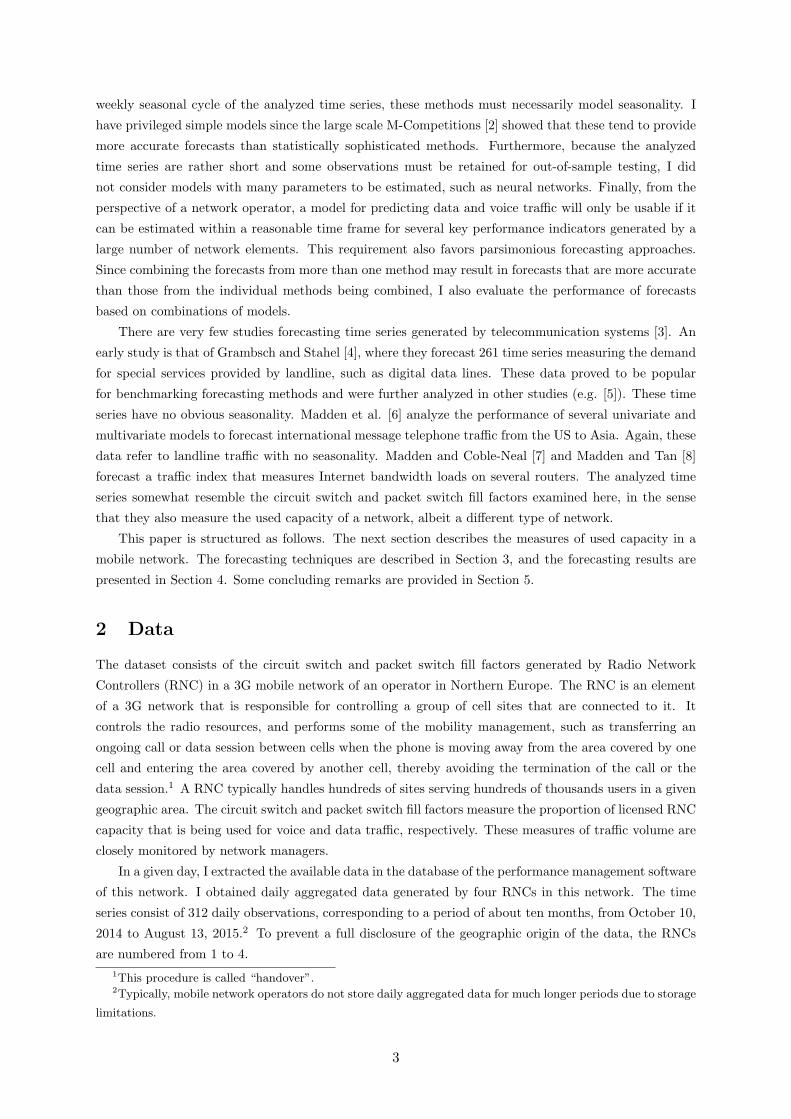
Figure 4: Comparison of root mean squared errors for voice traffic.

series is perfectly smoothed and corresponds to the trend line through the original data. In the M3

competition, two time series were constructed using θ = 0 and θ = 2 [13]. Then, the first is extrapolated

using a linear trend, while the second is extrapolated with a simple exponential smoothing model. The

final forecast is a simple average of the two forecasts. I also considered those values for θ. Hyndman and

Billah [14] show that this setup corresponds to a simple exponential smoothing model with an added

trend and a constant, where the slope of the trend is half that of the trend line through the initial

series. The theta model can also be applied to seasonal data after the series is deseasonalized. The

resultant forecasts are then reseasonalized before being used. This method performed very well in the

M3 competition.

4 Forecasting results

I evaluated out-of-sample accuracies using a rolling forecasting origin, with the training data being

successively augmented by one observation. The models are re-estimated every time the training sample

is incremented. This approach simulates the scenario where new data are collected and stored in the

network management system. I generated forecasts for a horizon of up to 28 days. The results shown

below refer to a test sample consisting of the last 120 days.

4.1 Accuracy measures

Several measures of forecast accuracy are available to compare the relative performance of the different

methods. The M3-competition showed that the relative ranking of competing methods depends on how

accuracy is measured. I considered two measures of accuracy: the root mean squared error (RMSE)

and the mean absolute percentage error (MAPE). Models with lower RMSE and MAPE have smaller

7

0 5 10 15 20 25

68

10

12

14

RNC1

Horizon (days)

Random walk

Linear trend

Theta


ARIMA

0 5 10 15 20 25

10

15

20

25

30

35

RNC2

Horizon (days)

Random walk

Linear trend

Theta


ARIMA

0 5 10 15 20 25

10

15

20

25

30

35

RNC3

Horizon (days)

Random walk

Linear trend

Theta


ARIMA

0 5 10 15 20 25

10

15

20

25

RNC4

Horizon (days)

Random walk

Linear trend

Theta


ARIMA

Figure 5: Comparison of mean absolute percentage errors for voice traffic.

differences between the actual and predicted values, and predict actual values more accurately. The

RMSE is more sensitive to large forecasting errors and, therefore, should be preferred when these are

particularly undesirable. Percentage errors have the appeal of being independent of the scale of the data.

4.2 Accuracy results

Figure 4 shows the out-of-sample RMSEs for voice traffic as a function of the forecast horizon. In general,

the random walk model ranks last in terms of performance. Exponential smoothing is the best model

for RNCs 1, 2 and 3, while the ARIMA model is the most accurate for RNC4. Sometimes, the linear

model does not perform better than the naıve random walk model. It is somewhat surprising that the

theta method does not rank very well, given its good performance in the M3 competition.

The out-of-sample MAPEs for voice traffic as a function of the forecast horizon are shown in Figure

5. The relative ranking of the methods changes when we consider this measure of forecasting accuracy.

The linear trend model performs very poorly in terms of this measure. Exponential smoothing is the

best model overall, being the only model that consistently outperforms the random walk. Surprisingly,

the ARIMA model does not perform better than the random walk for RNCs 1, 2 and 3. The performance

of the theta method is similar to that of the exponential smoothing method.

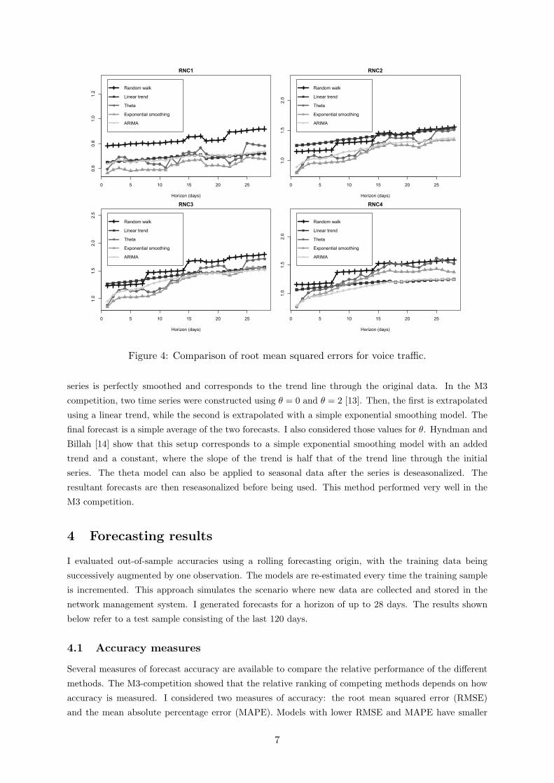
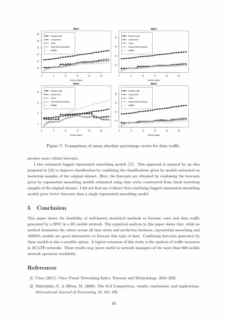
The relative ranking of the methods is rather different for data traffic. Figure 6 shows the the out-of-

sample RMSEs. The most surprising result is the poor performance of the linear trend model. For RNCs

1, 2 and 4, ARIMA is the best model across all forecasting horizons. For RNC 3, the most accurate

models are the exponential smoothing and theta models. Also, for this RNC the ARIMA model has very

poor performance for long term forecasts.

Finally, Figure 7 shows the out-of-sample MAPEs for data traffic. For this type of traffic, the

accuracies in terms of MAPE are qualitatively similar to the accuracies measured by RMSEs.

8

0 5 10 15 20 25

51

01

52

0

RNC1

Horizon (days)

Random walk

Linear trend

Theta


ARIMA

0 5 10 15 20 25

24

68

10

RNC2

Horizon (days)

Random walk

Linear trend

Theta


ARIMA

0 5 10 15 20 25

23

45

67

RNC3

Horizon (days)

Random walk

Linear trend

Theta


ARIMA

0 5 10 15 20 25

24

68

10

12

14

16

RNC4

Horizon (days)

Random walk

Linear trend

Theta


ARIMA

Figure 6: Comparison of root mean squared errors for data traffic.

4.3 Combining forecasts

Combining forecasts of more than one model may result in more accurate forecasts than those given

by the individual models [15]. Therefore, I examined whether combined forecasts provide lower errors

than those in subsection 4.2. I considered two combination strategies. The first combination strategy

neglects the historical performance of the individual methods, and gives equal and constant weights to

each forecast.4 The second combination strategy takes into account the past accuracy of each model,

giving higher weights to models with better accuracy. In this strategy, the weights were equal to the

inverse of the post-sample mean squared errors, which were incrementally updated as new forecasts were

generated.

I discarded the models with worst performance, and considered combinations of the exponential

smoothing and ARIMA models. Figure 8 shows the MAPEs for voice traffic given by the exponential

smoothing models, ARIMA models, and the combinations of these models. In general, the two combi-

nation strategies do not outperform the best model. Also, the combination strategy with distinct and

time varying weights is slightly better than combination strategy with equal weights.

Figure 9 shows the corresponding MAPEs for data traffic. The results are similar to those for voice

data. Again, the two combination strategies do not outperform the best model, and the combination

strategy with unequal weights is better than the combination strategy with equal weights. Still, combin-

ing forecasts from ARIMA and exponential smoothing methods may be a good approach for implementing

a real-time automatic forecasting framework. Since no model dominates the others across all time series

and forecast horizons, a network manager might prefer to combine forecasts from different models to

4There is some empirical evidence that a simple average of individual forecasts performs better than more

sophisticated combination methods [16].

9

0 5 10 15 20 25

10

20

30

40

50

60

RNC1

Horizon (days)

Random walk

Linear trend

Theta


ARIMA

0 5 10 15 20 25

10

20

30

40

RNC2

Horizon (days)

Random walk

Linear trend

Theta


ARIMA

0 5 10 15 20 25

46

81

0

RNC3

Horizon (days)

Random walk

Linear trend

Theta


ARIMA

0 5 10 15 20 25

10

20

30

40

RNC4

Horizon (days)

Random walk

Linear trend

Theta


ARIMA

Figure 7: Comparison of mean absolute percentage errors for data traffic.

produce more robust forecasts.

I also estimated bagged exponential smoothing models [17]. This approach is inspired by an idea

proposed in [18] to improve classification by combining the classifications given by models estimated on

bootstrap samples of the original dataset. Here, the forecasts are obtained by combining the forecasts

given by exponential smoothing models estimated using time series constructed from block bootstrap

samples of the original dataset. I did not find any evidence that combining bagged exponential smoothing

models gives better forecasts than a single exponential smoothing model.

5 Conclusion

This paper shows the feasibility of well-known statistical methods to forecast voice and data traffic

generated by a RNC in a 3G mobile network. The empirical analysis in this paper shows that, while no

method dominates the others across all time series and prediction horizons, exponential smoothing and

ARIMA models are good alternatives to forecast this type of data. Combining forecasts generated by

these models is also a sensible option. A logical extension of this study is the analysis of traffic measures

in 4G LTE networks. These results may prove useful to network managers of the more than 800 mobile

network operators worldwide.

References

[1] Cisco (2017). Cisco Visual Networking Index: Forecast and Methodology, 2016–2021.

[2] Makridakis, S., & Hibon, M. (2000). The M-3 Competition: results, conclusions, and implications.

International Journal of Forecasting, 16, 451–476.

10

0 5 10 15 20 25

56

78

91

01

11

2

RNC1

Horizon (days)


ARIMA

Combined ✁ equal weights

Combined ✁ unequal weights

0 5 10 15 20 25

10

15

20

25

RNC2

Horizon (days)


ARIMA



0 5 10 15 20 25

10

15

20

25

RNC3

Horizon (days)


ARIMA



0 5 10 15 20 25

10

15

20

RNC4

Horizon (days)


ARIMA



Figure 8: Mean absolute percentage errors for voice traffic given by the exponential smoothing

models, ARIMA models, and the combinations of these models.

[3] Meade, N., & Islam, T. (2015). Forecasting in telecommunications and ICT – A review. International

Journal of Forecasting, 31, 1105-1126.

[4] Grambsch, P., & Stahel, W.A. (1990). Forecasting demand for special telephone services – a case

study. International Journal of Forecasting, 6, 53–64.

[5] Fildes, R. (1992). The evaluation of extrapolative forecasting methods. International Journal of

Forecasting, 8, 81–98.

[6] Madden, G., Savage, S.J., & Coble-Neal, G. (2002). Forecasting United States-Asia international

message telephone service. International Journal of Forecasting, 18, 523–543.

[7] Madden, G., & Coble-Neal, G. (2005). Forecasting international bandwidth capability. Journal of

Forecasting, 24, 299–309.

[8] Madden, G., & Tan, J. (2008). Forecasting international bandwidth capacity using linear and ANN

methods. Applied Economics, 40, 1775–1787.

[9] Hyndman, R.J., O’Hara-Wild, M., Bergmeir, C., & Razbash, S. (2017). Package ‘forecast’, Septem-

ber 25, 2017.

[10] Gardner Jr., E.S. (2006). Exponential smoothing: The state of the art – Part II. International

Journal of Forecasting, 22, 637–666.

[11] Gardner Jr., E. S., & McKenzie, E. (1989). Seasonal exponential smoothing with damped trends.

Management Science, 35, 372–376.

11

0 5 10 15 20 25

51

01

52

02

53

0

RNC1

Horizon (days)


ARIMA


Combined ✁ different weights

0 5 10 15 20 25

46

81

01

21

41

6

RNC2

Horizon (days)


ARIMA



0 5 10 15 20 25

46

81

0

RNC3

Horizon (days)


ARIMA



0 5 10 15 20 25

68

10

12

14

16

RNC4

Horizon (days)


ARIMA



Figure 9: Mean absolute percentage errors for data traffic given by the exponential smoothing

models, ARIMA models, and the combinations of these models.

[12] Hyndman, R.J., & Khandakar, Y. (2008). Automatic time series forecasting: The forecast package

for R. Journal of Statistical Software, 26.

[13] Assimakopoulos, V., & Nikolopoulos, K. (2000). The theta model: a decomposition approach to

forecasting. International Journal of Forecasting, 16, 521–530.

[14] Hyndman, R.J., & Billah, B. (2003). Unmasking the theta method. International Journal of Fore-

casting, 19, 287–290.

[15] Timmermann, A. (2006). Forecast combinations. Elliott, G., Granger, C.W.J., Timmermann, A.

(Eds.), Handbook of Economic Forecasting, 135–196, Elsevier Press.

[16] Stock, J.H., & Watson, M.W. (2001). A comparison of linear and nonlinear univariate models for

forecasting macroeconomic time series. In Engle, R.F., White, H. (Eds.) Festschrift in Honour of

Clive Granger. Cambridge University press, Cambridge, 1–44.

[17] Bergmeir, C., Hyndman, R.J., & Benıtez, J. M. (2016). Bagging exponential smoothing methods

using STL decomposition and Box-Cox transformation. International Journal of Forecasting, 32,

303–312.

[18] Breiman, L. (1996). Bagging predictors. Machine Learning, 24, 123–140.

12

forecasting the capacity of mobile networks

Documents