forecasting the equity risk premium: the role of ... - cafr

MANAGEMENT SCIENCEVol. 60, No. 7, July 2014, pp. 1772–1791ISSN 0025-1909 (print) � ISSN 1526-5501 (online) http://dx.doi.org/10.1287/mnsc.2013.1838

© 2014 INFORMS

Forecasting the Equity Risk Premium:The Role of Technical Indicators

Christopher J. NeelyResearch Division, Federal Reserve Bank of St. Louis, St. Louis, Missouri 63166, [email protected]

David E. RapachDepartment of Economics, John Cook School of Business, Saint Louis University, St. Louis, Missouri 63108,

[email protected]

Jun TuDepartment of Finance, Lee Kong Chian School of Business, Singapore Management University, Singapore 178899,

[email protected]

Guofu ZhouOlin Business School, Washington University in St. Louis, St. Louis, Missouri 63130, CAFR and CUFE,

[email protected]

Academic research relies extensively on macroeconomic variables to forecast the U.S. equity risk premium, withrelatively little attention paid to the technical indicators widely employed by practitioners. Our paper fills this

gap by comparing the predictive ability of technical indicators with that of macroeconomic variables. Technicalindicators display statistically and economically significant in-sample and out-of-sample predictive power,matching or exceeding that of macroeconomic variables. Furthermore, technical indicators and macroeconomicvariables provide complementary information over the business cycle: technical indicators better detect the typicaldecline in the equity risk premium near business-cycle peaks, whereas macroeconomic variables more readily pickup the typical rise in the equity risk premium near cyclical troughs. Consistent with this behavior, we show thatcombining information from both technical indicators and macroeconomic variables significantly improves equityrisk premium forecasts versus using either type of information alone. Overall, the substantial countercyclicalfluctuations in the equity risk premium appear well captured by the combined information in technical indicatorsand macroeconomic variables.

Data, as supplemental material, are available at http://dx.doi.org/10.1287/mnsc.2013.1838.

Keywords : equity risk premium predictability; macroeconomic variables; moving averages; momentum; volume;sentiment; out-of-sample forecasts; asset allocation; business cycle

History : Received January 9, 2012; accepted August 29, 2013, by Wei Jiang, finance. Published online in Articles inAdvance March 4, 2014.

1. IntroductionNumerous studies report evidence of U.S. equity riskpremium predictability based on assorted macroeco-nomic variables, including valuation ratios, interestrates, and interest rate spreads; see Cochrane (2011) andRapach and Zhou (2013) for recent surveys. Relative tomacroeconomic variables (i.e., “economic fundamen-tals”), technical indicators have received significantlyless attention in the literature, despite their widespreaduse among practitioners (e.g., Schwager 1989, Lo andHasanhodzic 2010). Technical indicators rely on pastprice and volume patterns to identify price trendsbelieved to persist into the future. Existing studiesanalyze the profitability of trading strategies based ona variety of technical indicators, including filter rules(Fama and Blume 1966), moving averages (Brock et al.1992, Zhu and Zhou 2009), momentum (Conrad and

Kaul 1998, Ahn et al. 2003), and automated patternrecognition (Lo et al. 2000). These studies, however, donot specifically analyze how well technical indicatorsdirectly predict the equity risk premium, which is thefocus of the vast literature on equity risk premiumpredictability based on macroeconomic variables.

In this paper, we investigate the capacity of technicalindicators to directly forecast the equity risk premiumand compare their performance to that of macro-economic variables. In comparing the technical andmacroeconomic predictors, we generate all forecasts ina standard predictive regression framework, where theequity risk premium is regressed on a constant and thelag of a macroeconomic variable or technical indicator.To parsimoniously incorporate information from manypredictors, we also estimate predictive regressionsbased on a small number of principal components

1772

Dow

nloa

ded

from

info

rms.

org

by [

128.

252.

111.

81]

on 2

3 Ju

ly 2

014,

at 0

4:00

. Fo

r pe

rson

al u

se o

nly,

all

righ

ts r

eser

ved.

Neely et al.: Forecasting the Equity Risk PremiumManagement Science 60(7), pp. 1772–1791, © 2014 INFORMS 1773

extracted from the entire set of macroeconomic vari-ables and/or technical indicators. Our investigationcomplements existing studies of equity risk premiumpredictability, which ignore technical indicators, as wellas existing studies of technical indicators, which focuson the profitability of technical strategies.

We use data spanning from December 1950 to Decem-ber 2011 for 14 well-known macroeconomic variablesfrom the literature and 14 common technical indicators,including those based on moving averages, momentum,and volume. In-sample results demonstrate that indi-vidual technical indicators typically predict the equityrisk premium as well as, or better than, individualmacroeconomic variables. Regressions based on princi-pal components extracted from the 14 macroeconomicvariables (PC-ECON model) or 14 technical indicators(PC-TECH model) reveal that both macroeconomicvariables as a group and technical indicators as a groupsignificantly predict the equity risk premium. Moreover,the in-sample R2 statistic for a predictive regressionbased on principal components extracted from theentire set of macroeconomic variables and technicalindicators taken together (PC-ALL model) equals thesum of the R2 statistics for the PC-ECON and PC-TECH models. The additive nature of the predictabilityindicates that macroeconomic variables and technicalindicators capture different types of information rele-vant for predicting the equity risk premium and thusrepresent complementary approaches to equity riskpremium forecasting.

Consistent with differential information, the PC-ECON and PC-TECH model estimates of the expectedequity risk premium display complementary coun-tercyclical patterns. Technical indicators better detectthe typical decline in the actual equity risk premiumnear business-cycle peaks, whereas macroeconomicvariables more readily pick up the typical rise in theactual equity risk premium later in recessions nearcyclical troughs. The PC-ALL model estimate of theexpected equity risk premium exhibits an even clearercountercyclical pattern. This accentuated countercycli-cal pattern enables the expected equity risk premiumgenerated by the PC-ALL model to better track thesizable fluctuations in the actual equity risk premiumaround business-cycle peaks and troughs.

Out-of-sample results confirm the in-sample results.Forecast encompassing tests suggest that utilizinginformation from both macroeconomic variables andtechnical indicators can improve equity risk premiumforecasts. Indeed, the PC-ALL model performs the bestand significantly outperforms the historical averageforecast, which Goyal and Welch (2003, 2008) showto be a very stringent benchmark. Furthermore, thePC-ALL forecast has substantial economic value fora mean-variance investor with a relative risk coeffi-cient of five who optimally allocates across equities

and risk-free Treasury bills. In particular, the investorrealizes substantial utility gains by using the PC-ALLforecast versus ignoring any forecastability or usingthe information in macroeconomic variables alone.

Theoretically, why do macroeconomic variables andtechnical indicators predict the equity risk premium?In dynamic asset pricing models, the future state of theeconomy is the fundamental driver of time-varyingexpected stock returns. Macroeconomic variables trackchanging macroeconomic conditions and should thushave predictive power for the equity risk premium. Thispredictive ability reflects time-varying compensation toinvestors for bearing aggregate risk and is consistentwith rational asset pricing; see Cochrane (2011) andreferences therein. Explanations of the predictive powerof technical indicators are not as well known, however,and require more discussion. There are basically fourtypes of theoretical models that explain why technicalindicators can have predictive ability, all of which pointto an informationally inefficient market.

The first type of theoretical model recognizes differ-ences in the time for investors to receive information.Under this friction, Treynor and Ferguson (1985) showthat technical analysis is useful for assessing whetherinformation has been fully incorporated into equityprices, whereas Brown and Jennings (1989) demon-strate that past prices enable investors to make betterinferences about price signals. In addition, Grundy andMcNichols (1989) and Blume et al. (1994) show thattrading volume can provide useful information beyondprices.

The second type of model posits different responsesto information by heterogeneous investors. Cespa andVives (2012) recently show that asset prices can deviatefrom their fundamental values if there is a positive levelof asset residual payoff uncertainty and/or persistencein liquidity trading. In this setting, rational long-terminvestors follow trends. In the real world, differentresponses to information are more likely during reces-sions because of, for example, consumption-smoothingasset sales by households that experience job losses andliquidation sales of margined assets by some investors.These factors help to explain why we find that technicalindicators display enhanced predictive ability duringrecessions.

The next type of model allows for underreaction andoverreaction to information. Hong and Stein (1999)explain that, at the start of a trend, investors underreactto news because of behavioral biases; as the marketrises, investors subsequently overreact, leading to evenhigher prices. Similarly, positive feedback traders—whobuy (sell) after asset prices rise (fall)—can create pricetrends that technical indicators detect. Hedge fundguru Soros (2003) argues that positive feedback canactually alter firm fundamentals, thereby justifying toa certain extent the price trends. Edmans et al. (2012)

Dow

nloa

ded

from

info

rms.

org

by [

128.

252.

111.

81]

on 2

3 Ju

ly 2

014,

at 0

4:00

. Fo

r pe

rson

al u

se o

nly,

all

righ

ts r

eser

ved.

Neely et al.: Forecasting the Equity Risk Premium1774 Management Science 60(7), pp. 1772–1791, © 2014 INFORMS

recently show that such feedback trading can occur ina rational model of investors with private information.

Finally, models of investor sentiment shed light onthe efficacy of technical analysis. Since Keynes (1936),researchers have analyzed how investor sentiment candrive asset prices away from their fundamental values.DeLong et al. (1990) show that in the presence of limitsto arbitrage, noise traders with irrational sentiment cancause prices to deviate from their fundamentals, evenwhen informed traders recognize the mispricing. Bakerand Wurgler (2006, 2007) find that measures of investorsentiment help to explain the cross-section of U.S. equityreturns. In this paper, the monthly sentiment-changesindex from Baker and Wurgler (2007) is significantlyand positively contemporaneously correlated withthe realized equity risk premium, and we show thattechnical indicators significantly predict the sentiment-changes index, whereas macroeconomic variables donot. The differential information useful for predictingthe equity risk premium in technical indicators thusappears related to their ability to anticipate changes ininvestor sentiment.

In sum, theoretical models based on informationfrictions help to explain the predictive value of technicalindicators. Empirically, Moskowitz et al. (2012) recentlyfind that pervasive price trends exist across commonlytraded equity index, currency, commodity, and bondfutures. Insofar as the stock market is not a purerandom walk and exhibits periodic trends, technicalindicators should prove informative because they areprimarily designed to detect trends.

2. In-Sample Analysis2.1. Bivariate Predictive RegressionsThe conventional framework for analyzing equityrisk premium predictability based on macroeconomicvariables is the following predictive regression model:

rt+1 = �i +�ixi1 t + �i1 t+11 (1)

where the equity risk premium, rt+1, is the return on abroad stock market index in excess of the risk-free ratefrom period t to t+ 1; xi1 t is a predictor available att; and �i1 t+1 is a zero-mean disturbance term. Underthe null hypothesis of no predictability, �i = 0, and (1)reduces to the constant expected equity risk premiummodel. Because theory suggests the sign of �i, Inoueand Kilian (2004) recommend a one-sided alternativehypothesis to increase the power of in-sample tests ofpredictability; we define xi1 t such that �i is expected tobe positive under the alternative. We test H0: �i = 0against HA: �i > 0 using a heteroskedasticity-consistentt-statistic corresponding to �̂i, the ordinary least squares(OLS) estimate of �i in (1).

The well-known Stambaugh (1999) bias potentiallyinflates the t-statistic for �̂i in (1) and distorts test

size when xi1 t is highly persistent, as is the case for anumber of popular predictors. We address this con-cern by computing p-values using a wild bootstrapprocedure that accounts for the persistence in regres-sors and correlations between equity risk premiumand predictor innovations as well as general forms ofheteroskedasticity. The online appendix (available athttp://sites.slu.edu/rapachde/home/research) accom-panying this paper details the wild bootstrap procedure.

We estimate predictive regressions using updatedmonthly data from Goyal and Welch (2008).1 The equityrisk premium is the difference between the log returnon the S&P 500 (including dividends) and the log returnon a risk-free bill. The following 14 macroeconomicvariables are representative of the literature (Goyal andWelch 2008) and constitute the set of xi1 t variables usedto predict the equity risk premium in (1):

1. Dividend-price ratio (log), DP: log of a 12-monthmoving sum of dividends paid on the S&P 500 Indexminus the log of stock prices (S&P 500 Index).

2. Dividend yield (log), DY: log of a 12-month mov-ing sum of dividends minus the log of lagged stockprices.

3. Earnings-price ratio (log), EP: log of a 12-monthmoving sum of earnings on the S&P 500 Index minusthe log of stock prices.

4. Dividend-payout ratio (log), DE: log of a 12-monthmoving sum of dividends minus the log of a 12-monthmoving sum of earnings.

5. Equity risk premium volatility, RVOL: basedon a 12-month moving standard deviation estimator(Mele 2007).2

6. Book-to-market ratio, BM: book-to-market valueratio for the Dow Jones Industrial Average.

7. Net equity expansion, NTIS: ratio of a 12-monthmoving sum of net equity issues by NYSE-listed stocksto the total end-of-year market capitalization of NewYork Stock Exchange (NYSE) stocks.

8. Treasury bill rate, TBL: interest rate on a three-month Treasury bill (secondary market).

9. Long-term yield, LTY: long-term government bondyield.

10. Long-term return, LTR: return on long-termgovernment bonds.

11. Term spread, TMS: long-term yield minus theTreasury bill rate.

12. Default yield spread, DFY: difference betweenMoody’s BAA- and AAA-rated corporate bond yields.

1 The data are available from Amit Goyal’s webpage at http://www.hec.unil.ch/agoyal/.2 Goyal and Welch (2008) measure monthly volatility as the sum ofsquared daily excess stock returns during the month. This measure,however, produces a severe outlier in October 1987. The Mele (2007)measure avoids this problem and yields more plausible estimationresults.

Dow

nloa

ded

from

info

rms.

org

by [

128.

252.

111.

81]

on 2

3 Ju

ly 2

014,

at 0

4:00

. Fo

r pe

rson

al u

se o

nly,

all

righ

ts r

eser

ved.


13. Default return spread, DFR: long-term corporatebond return minus the long-term government bondreturn.

14. Inflation, INFL: calculated from the CPI for allurban consumers; we use xi1 t−1 in (1) for inflation toaccount for the delay in CPI releases.

Table 1 reports summary statistics for the equity riskpremium and 14 macroeconomic variables for Decem-ber 1950 to December 2011. The start of the samplereflects data availability for the technical indicators(discussed below). The average monthly equity riskpremium is 0.47%, which, together with a monthly stan-dard deviation of 4.26%, produces a monthly Sharperatio of 0.11. Most of the macroeconomic variablesare strongly autocorrelated, particularly the valuationratios, nominal interest rates, and interest rate spreads.

To compare technical indicators to the macroeco-nomic variables, we employ 14 technical indicatorsbased on three popular trend-following strategies. Thefirst is a moving-average (MA) rule that generates abuy or sell signal (Si1 t = 1 or Si1 t = 0, respectively) atthe end of t by comparing two moving averages:

Si1 t =

{

1 if MAs1 t ≥ MAl1 t1

0 if MAs1 t < MAl1 t1(2)

where

MAj1 t = 41/j5j−1∑

i=0

Pt−i for j = s1 l3 (3)

Pt is the level of a stock price index, and s (l) is thelength of the short (long) MA (s < l). We denote theMA indicator with MA lengths s and l by MA(s1 l).

Table 1 Summary Statistics, December 1950 to December 2011

Std. Auto- SharpeVariable Mean dev. Min Max correlation ratio

Log equity 0047 4.26 −24084 14087 0006 0.11risk premium

DP −3049 0.42 −4052 −2060 0099DY −3048 0.42 −4053 −2059 0099EP −2078 0.44 −4084 −1090 0099DE −0071 0.30 −1024 1038 0099RVOL 0014 0.05 0005 0032 0096BM 0054 0.25 0012 1021 0099NTIS 0002 0.02 −0006 0005 0098TBL 4067 2.95 0001 16030 0099LTY 6032 2.68 2021 14082 0099LTR 0056 2.76 −11024 15023 0005TMS 1064 1.42 −3065 4055 0096DFY 0096 0.45 0032 3038 0097DFR 0001 1.38 −9075 7037 −0009INFL 0030 0.35 −1092 1079 0061

Notes. This table reports summary statistics for the log equity risk premium(in percent) and 14 macroeconomic variables. LTR, DFR, and INFL (TBL, LTY,TMS, and DFY) are measured in percent (annual percent). The Sharpe ratio isthe mean of the log equity risk premium divided by its standard deviation.

Intuitively, the MA rule detects changes in stock pricetrends because the short MA will be more sensitiveto recent price movement than will the long MA. Weanalyze monthly MA rules with s = 11213 and l = 9112.

The second strategy is based on momentum. A simplemomentum rule generates the following signal:

Si1 t =

{

1 if Pt ≥ Pt−m1

0 if Pt <Pt−m0(4)

Intuitively, a current stock price that is higher than itslevel m periods ago indicates “positive” momentumand relatively high expected excess returns, therebygenerating a buy signal. We denote the momentumindicator that compares Pt to Pt−m by MOM(m), andwe compute monthly signals for m= 9112.

Technical analysts frequently employ volume datain conjunction with past prices to identify markettrends. In light of this, the final strategy we considerincorporates “on-balance” volume (e.g., Granville 1963).We first define

OBVt =

t∑

k=1

VOLkDk1 (5)

where VOLk is a measure of the trading volume duringperiod k and Dk is a binary variable that takes a valueof 1 if Pk − Pk−1 ≥ 0 and −1 otherwise. We then form atrading signal from OBVt as

Si1 t =

1 if MAOBVs1 t ≥ MAOBV

l1 t 1

0 if MAOBVs1 t < MAOBV

l1 t 1(6)

where

MAOBVj1 t = 41/j5

j−1∑

i=0

OBVt−i for j = s1 l0 (7)

Intuitively, relatively high recent volume together withrecent price increases, say, indicate a strong positivemarket trend and generate a buy signal. We computemonthly signals for s = 11213 and l = 9112 and denotethe corresponding indicator by VOL(s1 l).

The MA, momentum, and volume-based indicatorsare representative of the trend-following technicalindicators analyzed in the academic literature (e.g.,Sullivan et al. 1999). We use the S&P 500 Index andmonthly volume data from Google Finance in (2), (4),and (6).3 After accounting for the lags in constructingthe technical indicators, we have observations for all ofthe indicators starting in December 1950.4 The technical

3 The volume data are available at http://www.google.com/finance.4 Technical indicators are often computed using monthly, weekly, ordaily data. We compute technical indicators using monthly data toput the forecasts based on macroeconomic variables and technicalindicators on a more equal footing.

Dow

nloa

ded

from

info

rms.

org

by [

128.

252.

111.

81]

on 2

3 Ju

ly 2

014,

at 0

4:00

. Fo

r pe

rson

al u

se o

nly,

all

righ

ts r

eser

ved.


Table 2 Predictive Regression Estimation Results, January 1951 to December 2011

Macroeconomic variables Technical indicators

Slope SlopePredictor coefficient R2 (%) R2

EXP (%) R2REC (%) Predictor coefficient R2 (%) R2

EXP (%) R2REC (%)

Panel A: Bivariate predictive regressionsDP 0.78 [1.98] 0.58 0040 1000 MA(1, 9) 0.67 [1.78]∗∗ 0.54 −0039 2.66DY 0.84 [2.13]∗∗ 0.67 0032 1048 MA(1, 12) 0.87 [2.22]∗∗ 0.87 −0018 3.27EP 0.43 [0.97] 0.20 0022 0014 MA(2, 9) 0.70 [1.88]∗∗ 0.59 −0026 2.53DE 0.59 [0.93] 0.17 0009 0035 MA(2, 12) 0.94 [2.42]∗∗∗ 1.03 −0009 3.58RVOL 7.41 [2.45]∗∗∗ 0.73 0054 1018 MA(3, 9) 0.77 [2.04]∗∗ 0.69 0003 2.22BM 0.54 [0.75] 0.10 0001 0029 MA(3, 12) 0.54 [1.39]∗ 0.34 −0012 1.39NTIS 0.66 [0.06] 0.00 0004 −0008 MOM(9) 0.55 [1.40]∗ 0.34 −0009 1.33TBL 0.11 [1.90]∗∗ 0.56 0042 0090 MOM(12) 0.58 [1.45]∗ 0.37 −0036 2.04LTY 0.08 [1.25]∗∗ 0.23 0022 0023 VOL(1, 9) 0.68 [1.86]∗∗ 0.56 −0051 3.02LTR 0.13 [2.05]∗∗ 0.76 −0041 3041 VOL(1, 12) 0.89 [2.31]∗∗∗ 0.92 −0020 3.49TMS 0.20 [1.74]∗∗ 0.44 0003 1038 VOL(2, 9) 0.74 [2.02]∗∗ 0.67 −0017 2.58DFY 0.16 [0.37] 0.03 0004 0000 VOL(2, 12) 0.74 [1.94]∗∗ 0.65 −0004 2.21DFR 0.16 [0.89] 0.26 0005 0074 VOL(3, 9) 0.48 [1.27] 0.27 −0017 1.29INFL 0.10 [0.18] 0.01 0007 −0014 VOL(3, 12) 0.85 [2.25]∗∗∗ 0.85 0021 2.30

Panel B: Principal component predictive regressions

F̂ ECON1 0.04 [0.48] 1.18 0079 2007 F̂ TECH

1 0.12 [2.12]∗∗ 0.84 −0019 3.18F̂ ECON

2 0.07 [0.61]F̂ ECON

3 0.31 [2.48]∗∗∗

Panel C: Principal component predictive regression, all predictors taken together

F̂ ALL1 0.11 [1.98]∗∗ 2.02 0029 5095F̂ ALL

2 0.08 [0.93]F̂ ALL

3 0.18 [1.51]∗

F̂ ALL4 0.26 [2.30]∗∗∗

Notes. Panel A reports estimation results for the bivariate predictive regression model,

rt+1 = �i + �iqi1 t + �i1 t+11

where rt+1 is the log equity risk premium (in percent) and qi1 t is one of the 14 macroeconomic variables (14 technical indicators) given in the first (sixth) column.Panels B and C report estimation results for a predictive regression model based on principal components,

rt+1 = �+

K∑

k=1

�k F̂jk1 t + �t+11

where F̂ jk1 t is the kth principal component extracted from the 14 macroeconomic variables (j = ECON), 14 technical indicators (j = TECH), or the 14 macroeconomic

variables and 14 technical indicators taken together (j = ALL). We select K via the adjusted R2. The brackets to the immediate right of the estimated slopecoefficients report heteroskedasticity-consistent t-statistics. The R2 statistics in the third and eighth columns are computed for the full sample. The R2

EXP (R2REC)

statistics in the fourth and ninth (fifth and tenth) columns are computed for National Bureau of Economic Research-dated business-cycle expansions (recessions),as given by (9) in the text.

∗, ∗∗, and ∗∗∗ indicate significance at the 10%, 5%, and 1% levels, respectively, based on one-sided (upper-tail) wild bootstrapped p-values; 0.00 indicates lessthan 0.005 in absolute value.

indicators generate buy signals (Si1 t = 1) between 66%and 72% of the time.

To directly compare these technical indicators toequity risk premium forecasts based on macroeconomicvariables, we transform the technical indicators to pointforecasts of the equity risk premium by replacing xi1 tin (1) with Si1 t from (2), (4), or (6):

rt+1 = �i +�iSi1 t + �i1 t+10 (8)

Because Si1 t = 1 (Si1 t = 0) represents a bullish (bearish)signal, we again test H0: �i = 0 against HA: �i > 0.

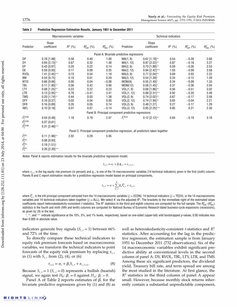
Panel A of Table 2 reports estimates of �i for thebivariate predictive regressions given by (1) and (8) as

well as heteroskedasticity-consistent t-statistics and R2

statistics. After accounting for the lag in the predic-tive regression, the estimation sample is from January1951 to December 2011 (732 observations). Six of the14 macroeconomic variables exhibit significant pre-dictive ability at conventional levels in the secondcolumn of panel A: DY, RVOL, TBL, LTY, LTR, and TMS.Among these six significant predictors, the dividendyield, Treasury bill rate, and term spread are amongthe most studied in the literature. At first glance, theR2 statistics in the third column of panel A appearsmall. However, because monthly stock returns inher-ently contain a substantial unpredictable component,

Dow

nloa

ded

from

info

rms.

org

by [

128.

252.

111.

81]

on 2

3 Ju

ly 2

014,

at 0

4:00

. Fo

r pe

rson

al u

se o

nly,

all

righ

ts r

eser

ved.


a monthly R2 near 0.5% can represent an economicallysignificant degree of equity risk premium predictability(e.g., Campbell and Thompson 2008). Five of the R2

statistics in the third column of panel A exceed this0.5% benchmark.

Turning to the results for the technical indicators,13 of the 14 indicators evince significant predictiveability at conventional levels in the seventh columnof Table 2, panel A. The coefficient estimates indicatethat a buy signal predicts that the next month’s equityrisk premium is higher by 48 to 94 basis points thanwhen there is a sell signal. In addition, 10 of the 14 R2

statistics in the eighth column of panel A are abovethe 0.5% threshold, and the R2 for MA(2, 12) is 1.03%,which is the largest R2 in panel A. Overall, the in-sample bivariate regression results in panel A of Table 2suggest that individual technical indicators generallypredict the equity risk premium as well as, or betterthan, individual macroeconomic variables.

We are interested in gauging the relative strength ofequity risk premium predictability during NationalBureau of Economic Research (NBER)-dated business-cycle expansions and recessions. Computing R2 statis-tics separately for cyclical expansions and recessions isthe most natural way to proceed. Because of the natureof the R2 statistic, however, there is no clean decompo-sition of the full-sample R2 statistic into subsample R2

statistics based on the full-sample parameter estimates.To compare the degree of return predictability acrossexpansions and recessions, we compute the followingintuitive versions of the conventional R2 statistic:

R2c = 1 −

∑Tt=1 I

ct �̂

2i1 t

∑Tt=1 I

ct 4rt − r̄ 52

for c = EXP1 REC1 (9)

where IEXPt (IREC

t ) is an indicator variable that takes avalue of unity when month t is an expansion (recession)and zero otherwise, �̂i1 t is the fitted residual based onthe full-sample estimates of the predictive regressionmodel in (1) or (8), r̄ is the full-sample mean of rt , andT is the number of usable observations for the fullsample. Observe that, unlike the full-sample R2 statistic,the R2

EXP and R2REC statistics can be negative. The fourth

and fifth columns of panel A in Table 2 indicate thatequity risk premium predictability is substantiallyhigher for recessions vis-à-vis expansions for a numberof the macroeconomic variables, including DP, DY,RVOL, TBL, LTR, TMS, and DFR. According to thelast two columns of panel A, predictability is highlyconcentrated during recessions for all of the technicalindicators.

2.2. Predictive Regressions Based onPrincipal Components

Next, we incorporate information from multiplemacroeconomic variables by estimating a predictive

regression based on principal components.5 Let xt =4x11 t1 0 0 0 1 xN1 t5

′ denote the N -vector (N = 14) of theentire set of macroeconomic variables and let F̂ ECON

t =

4F̂ ECON11 t 1 0 0 0 1 F̂ ECON

K1 t 5′ denote the vector containing thefirst K principal components extracted from xt (whereK �N ). The principal component predictive regression(PC-ECON model) is given by

rt+1 = �+

K∑

k=1

�kF̂ECONk1 t + �t+10 (10)

Principal components parsimoniously incorporate infor-mation from a large number of potential predictors ina predictive regression. The first few principal com-ponents identify the key comovements among theentire set of predictors, which filters out much of thenoise in individual predictors, thereby guarding againstin-sample overfitting. Following convention, we stan-dardize the individual predictors before computing theprincipal components.

We again estimate (10) via OLS, computeheteroskedasticity-consistent t-statistics, and base infer-ences on wild bootstrapped p-values. The first fivecolumns of panel B in Table 2 report estimation resultsfor (10) with K = 3, the value selected by the adjustedR2.6 The coefficient estimate on the third principalcomponent is significant at the 1% level. The R2 for thePC-ECON model is 1.18%, which is greater than the0.5% benchmark. The R2

EXP and R2REC statistics indicate

that equity risk premium predictability is more thantwice as large for recessions compared to expansions.

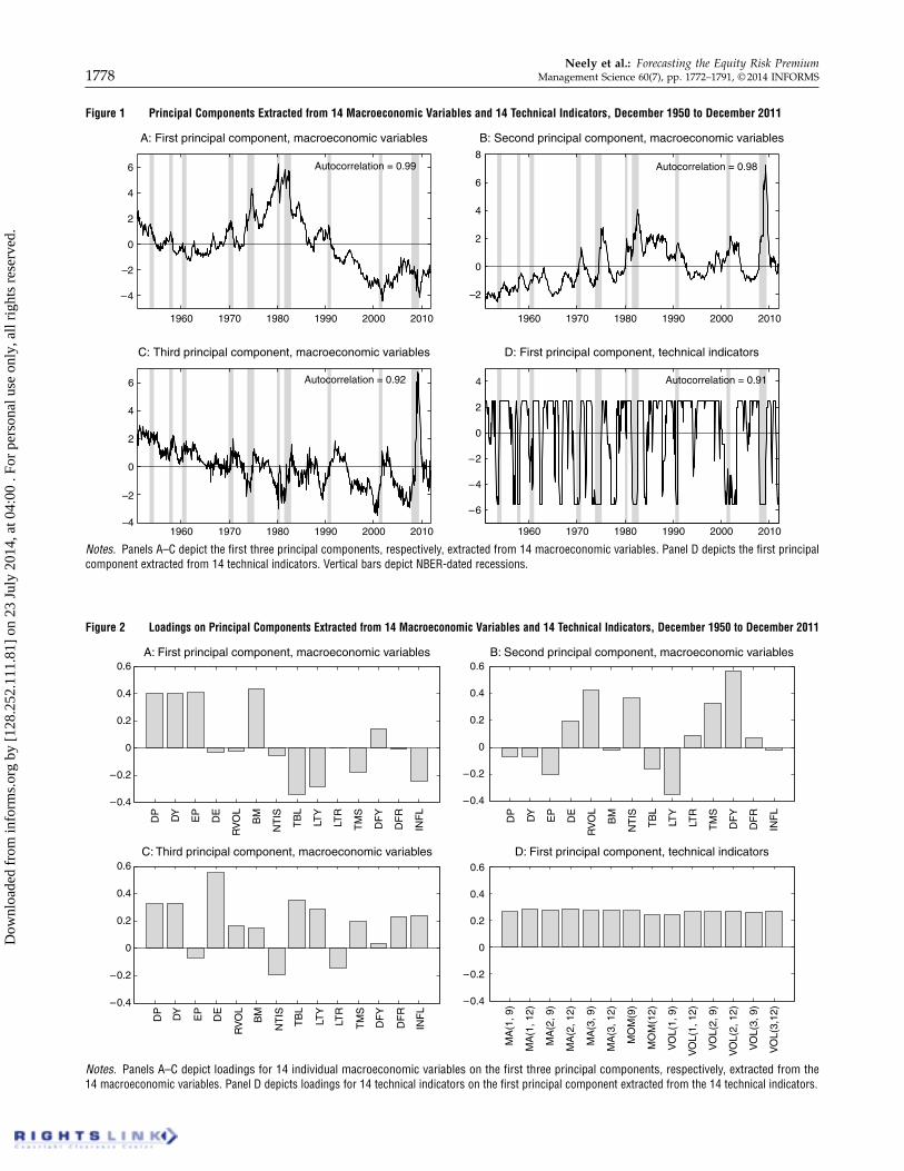
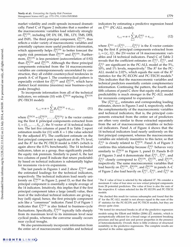
To illustrate the economic content of the princi-pal components, panels A–C of Figure 1 present theestimated principal components (8F̂ ECON

k1 t 93k=1), and the

corresponding panels in Figure 2 display the estimatedloadings for the individual macroeconomic variables onthe principal components. Panel A of Figure 2 showsthat the valuation ratios (DP, EY, EP, and BM) loadheavily on F̂ ECON

11 t ; that is, the first principal componentextracted from the macroeconomic variables primarilycaptures common fluctuations in the valuation ratios.This is also evident in Figure 1, panel A, where thepersistence of F̂ ECON

11 t (autocorrelation of 0.99) matchesthat of the individual valuation ratios in Table 1. FromFigure 2, panel B, we see that RVOL and DFY load mostheavily on F̂ ECON

21 t ; accordingly, F̂ ECON21 t spikes during the

global financial crisis in Figure 1, panel B, when stock

5 Ludvigson and Ng (2007, 2009) estimate predictive regressionsfor excess stock and bond returns, respectively, based on principalcomponents extracted from macroeconomic variables.6 The Akaike information criterion also selects K = 3. To keep themodel reasonably parsimonious, we consider a maximum K value ofthree, given the 14 macroeconomic variables. Note that we account forthe “estimated regressors” in (10) via the wild bootstrap procedure(as explained in the online appendix).

Dow

nloa

ded

from

info

rms.

org

by [

128.

252.

111.

81]

on 2

3 Ju

ly 2

014,

at 0

4:00

. Fo

r pe

rson

al u

se o

nly,

all

righ

ts r

eser

ved.


Figure 1 Principal Components Extracted from 14 Macroeconomic Variables and 14 Technical Indicators, December 1950 to December 2011

1960 1970 1980 1990 2000 2010

0

2

4

6

A: First principal component, macroeconomic variables

1960 1970 1980 1990 2000 2010

0

2

4

6

8

B: Second principal component, macroeconomic variables

1960 1970 1980 1990 2000 2010

0

–2

–2

–2–4

–4

2

4

6

C: Third principal component, macroeconomic variables

1960 1970 1980 1990 2000 2010

0

–2

–4

–6

2

4

D: First principal component, technical indicators

Autocorrelation = 0.99 Autocorrelation = 0.98


Notes. Panels A–C depict the first three principal components, respectively, extracted from 14 macroeconomic variables. Panel D depicts the first principalcomponent extracted from 14 technical indicators. Vertical bars depict NBER-dated recessions.

Figure 2 Loadings on Principal Components Extracted from 14 Macroeconomic Variables and 14 Technical Indicators, December 1950 to December 2011

0

0.2

0.4

0.6A: First principal component, macroeconomic variables

DP

DY

EP

DE

RV

OL

BM

NT

IS

TB

L

LTY

LTR

TM

S

DF

Y

DF

R

INF

L

0

0.2

0.4

0.6B: Second principal component, macroeconomic variables

DP

DY

EP

DE

RV

OL

BM

NT

IS

TB

L

LTY

LTR

TM

S

DF

Y

DF

R

INF

L

0

0.2

0.4

0.6C: Third principal component, macroeconomic variables

DP

DY

EP

DE

RV

OL

BM

NT

IS

TB

L

LTY

LTR

TM

S

DF

Y

DF

R

INF

L

0

0.2

–0.2

–0.4

–0.2

–0.4

–0.2

–0.4

–0.2

–0.4

0.4

0.6

D: First principal component, technical indicators

MA

(1, 9

)

MA

(1, 1

2)

MA

(2, 9

)

MA

(2, 1

2)

MA

(3, 9

)

MA

(3, 1

2)

MO

M(9

)

MO

M(1

2)

VO

L(1,

9)

VO

L(1,

12)

VO

L(2,

9)

VO

L(2,

12)

VO

L(3,

9)

VO

L(3,

12)

Notes. Panels A–C depict loadings for 14 individual macroeconomic variables on the first three principal components, respectively, extracted from the14 macroeconomic variables. Panel D depicts loadings for 14 technical indicators on the first principal component extracted from the 14 technical indicators.

Dow

nloa

ded

from

info

rms.

org

by [

128.

252.

111.

81]

on 2

3 Ju

ly 2

014,

at 0

4:00

. Fo

r pe

rson

al u

se o

nly,

all

righ

ts r

eser

ved.


market volatility and credit spreads increased dramati-cally. Panel C of Figure 2 indicates that a number ofthe macroeconomic variables load relatively stronglyon F̂ ECON

31 t , including DP, DY, DE, TBL, LTY, TMS, DFR,and INFL. The third principal component, F̂ ECON

31 t , thusreflects a wider variety of macroeconomic variables andpotentially captures more useful predictive information,which apparently helps F̂ ECON

31 t to better forecast theequity risk premium than F̂ ECON

11 t and F̂ ECON21 t . Further-

more, F̂ ECON31 t is less persistent (autocorrelation of 0.92)

than F̂ ECON11 t and F̂ ECON

21 t . Although the three principalcomponents extracted from the 14 macroeconomicvariables are contemporaneously uncorrelated by con-struction, they all exhibit countercyclical tendencies inpanels A–C of Figure 1. The countercyclical pattern isespecially evident for F̂ ECON

21 t and F̂ ECON31 t , which have

distinct local minima (maxima) near business-cyclepeaks (troughs).

To incorporate information from all of the technicalindicators, we estimate (10) with F̂ TECH

t replacing F̂ ECONt

(PC-TECH model):

rt+1 = �+

K∑

k=1

�kF̂TECHk1 t + �t+11 (11)

where F̂ TECHt = 4F̂ TECH

11 t 1 0 0 0 1 F̂ TECHK1 t 5′ is the vector contain-

ing the first K principal components extracted fromSt = 4S11 t1 0 0 0 1 SN1 t5

′, the N -vector of 14 technical indica-tors. The last five columns of panel B in Table 2 reportestimation results for (11) with K = 1 (the value selectedby the adjusted R2). The coefficient estimate on thefirst principal component is significant at the 5% level,and the R2 for the PC-TECH model is 0.84% (which isagain above the 0.5% benchmark). The 14 technicalindicators, taken as a group, thus significantly predictthe equity risk premium. Similarly to panel A, the lasttwo columns of panel B indicate that return predictabil-ity based on technical indicators is substantially higherfor recessions vis-à-vis expansions.

The last panels in Figures 1 and 2 show F̂ TECH11 t and

the estimated loadings for the technical indicators,respectively. The technical indicators load nearly uni-formly on F̂ TECH

11 t in Figure 2, panel D, so that the firstprincipal component is essentially a simple average ofthe 14 indicators. Intuitively, this implies that if the firstprincipal component takes a large (small) value, thenmost of the individual technical indicators are giving abuy (sell) signal; hence, the first principle componentacts like a “consensus” indicator. Panel D of Figure 1indicates that F̂ TECH

11 t is also linked to business-cyclefluctuations. Specifically, F̂ TECH

11 t typically falls sharplyfrom its maximum level to its minimum level nearcyclical peaks, whereas the converse usually occursnear cyclical troughs.

We also parsimoniously incorporate information fromthe entire set of macroeconomic variables and technical

indicators by estimating a predictive regression basedon F̂ ALL

t (PC-ALL model):

rt+1 = �+

K∑

k=1

�kF̂ALLk1 t + �t+11 (12)

where F̂ ALLt = 4F̂ ALL

11 t 1 0 0 0 1 F̂ ALLK1 t 5′ is the K-vector contain-

ing the first K principal components extracted fromzt = 4x′

t1 S′t5

′, the 2N -vector of 14 macroeconomic vari-ables and 14 technical indicators. Panel C of Table 2reveals that the coefficient estimates on F̂ ALL

11 t , F̂ ALL31 t , and

F̂ ALL41 t are significant in the PC-ALL model at the 5%,

10%, and 1% levels, respectively.7 The R2 for the PC-ALL model is 2.02%, which equals the sum of the R2

statistics for the PC-ECON and PC-TECH models.8

This indicates that the macroeconomic variables andtechnical predictors essentially contain complementaryinformation. Continuing the pattern, the fourth andfifth columns of panel C show that equity risk premiumpredictability is much stronger in the PC-ALL modelfor recessions compared to expansions.9

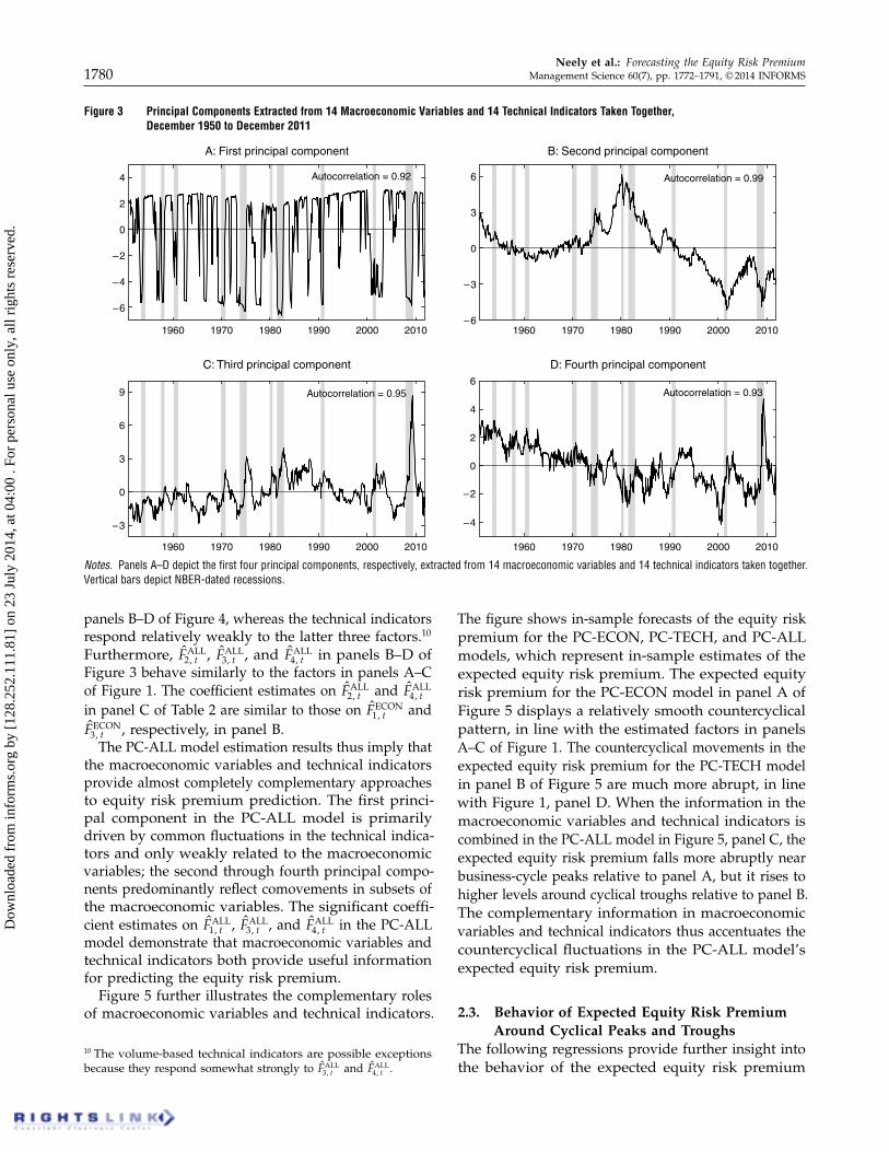
The 8F̂ ALLk1 t 94

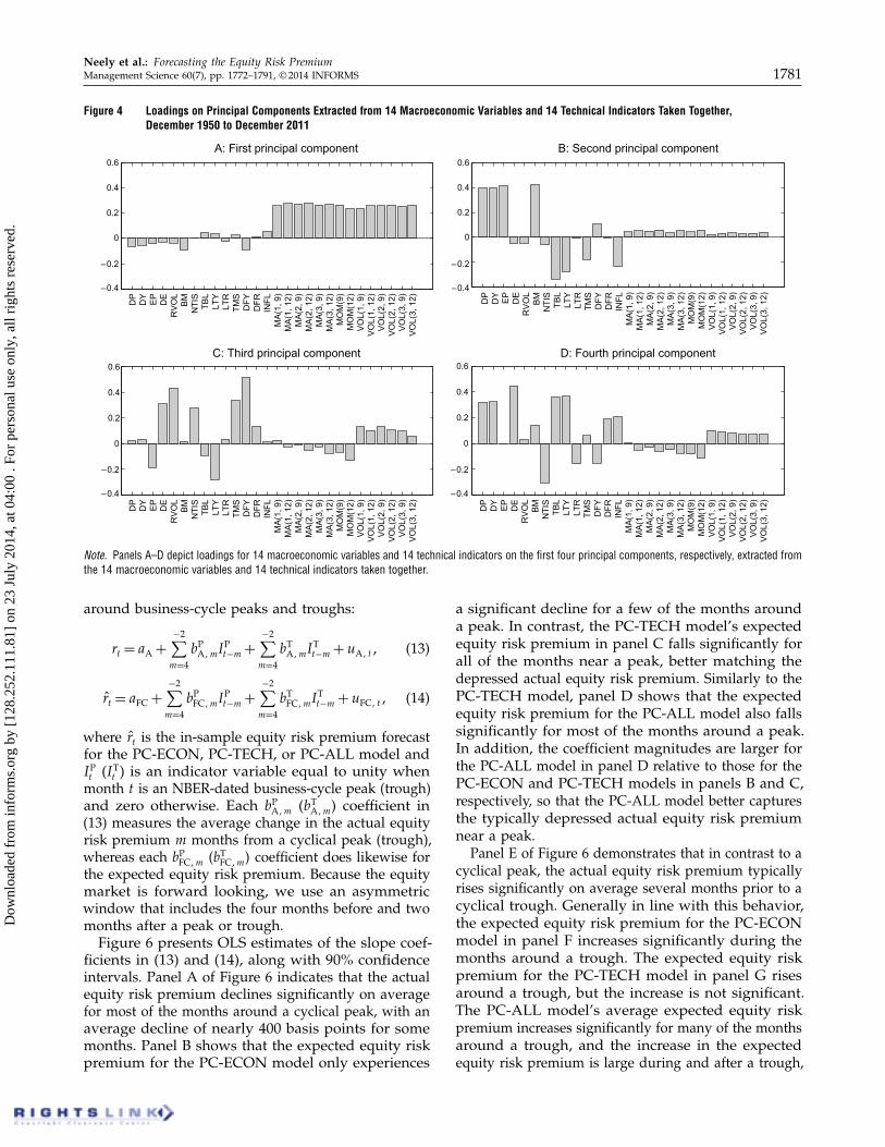
k=1 estimates and corresponding loadingestimates, shown in Figures 3 and 4, respectively, reflectthe complementarity of the macroeconomic variablesand technical indicators; that is, the principal com-ponents extracted from the entire set of predictorsare often very similar to those extracted separatelyfrom the set of macroeconomic variables or techni-cal indicators. Panel A of Figure 4 shows that the14 technical indicators load nearly uniformly on thefirst principal component, whereas the macroeconomicvariables are relatively insensitive to this factor, so thatF̂ ALL

11 t is closely related to F̂ TECH11 t . Panel A of Figure 3

confirms this relationship because F̂ ALL11 t behaves very

similarly to F̂ TECH11 t in Figure 1, panel D. Panels B–D

of Figures 3 and 4 demonstrate that F̂ ALL21 t , F̂ ALL

31 t , andF̂ ALL

41 t closely correspond to F̂ ECON11 t , F̂ ECON

21 t , and F̂ ECON31 t ,

respectively. The same macroeconomic variables thatload heavily on F̂ ECON

11 t , F̂ ECON21 t , and F̂ ECON

31 t in panels A–Cof Figure 2 also load heavily on F̂ ALL

21 t , F̂ ALL31 t , and F̂ ALL

41 t in

7 The K value of four is selected by the adjusted R2. We consider amaximum K value of four since we now extract principal componentsfrom 28 potential predictors. The value of four is also the sum ofthe respective K values selected for the PC-ECON and PC-TECHmodels.8 We checked this result for various subsamples and found that theR2 for the PC-ALL model is not always equal to the sum of theR2 statistics for the PC-ECON and PC-TECH models, but they arealways quite close.9 We tested for structural breaks in all of the predictive regression

models using the Elliott and Müller (2006) ̂qLL statistic, which isasymptotically efficient for a broad range of persistent breakingprocesses and has good size and power properties in the presenceof heteroskedasticity. Overall, there is little evidence of structuralinstability in the predictive regressions. The complete results arereported in the online appendix.

Dow

nloa

ded

from

info

rms.

org

by [

128.

252.

111.

81]

on 2

3 Ju

ly 2

014,

at 0

4:00

. Fo

r pe

rson

al u

se o

nly,

all

righ

ts r

eser

ved.


Figure 3 Principal Components Extracted from 14 Macroeconomic Variables and 14 Technical Indicators Taken Together,December 1950 to December 2011

1960 1970 1980 1990 2000 2010

0

2

4

A: First principal component

1960 1970 1980 1990 2000 2010

0

–3

–2

–4

–6–6

3

6

B: Second principal component

1960 1970 1980 1990 2000 2010

0

–3

–2

–4

3

6

9

C: Third principal component

1960 1970 1980 1990 2000 2010

0

2

4

6

D: Fourth principal component

Autocorrelation = 0.95


Autocorrelation = 0.93

Notes. Panels A–D depict the first four principal components, respectively, extracted from 14 macroeconomic variables and 14 technical indicators taken together.Vertical bars depict NBER-dated recessions.

panels B–D of Figure 4, whereas the technical indicatorsrespond relatively weakly to the latter three factors.10

Furthermore, F̂ ALL21 t , F̂ ALL

31 t , and F̂ ALL41 t in panels B–D of

Figure 3 behave similarly to the factors in panels A–Cof Figure 1. The coefficient estimates on F̂ ALL

21 t and F̂ ALL41 t

in panel C of Table 2 are similar to those on F̂ ECON11 t and

F̂ ECON31 t , respectively, in panel B.

The PC-ALL model estimation results thus imply thatthe macroeconomic variables and technical indicatorsprovide almost completely complementary approachesto equity risk premium prediction. The first princi-pal component in the PC-ALL model is primarilydriven by common fluctuations in the technical indica-tors and only weakly related to the macroeconomicvariables; the second through fourth principal compo-nents predominantly reflect comovements in subsets ofthe macroeconomic variables. The significant coeffi-cient estimates on F̂ ALL

11 t , F̂ ALL31 t , and F̂ ALL

41 t in the PC-ALLmodel demonstrate that macroeconomic variables andtechnical indicators both provide useful informationfor predicting the equity risk premium.

Figure 5 further illustrates the complementary rolesof macroeconomic variables and technical indicators.

10 The volume-based technical indicators are possible exceptionsbecause they respond somewhat strongly to F̂ ALL

31 t and F̂ ALL41 t .

The figure shows in-sample forecasts of the equity riskpremium for the PC-ECON, PC-TECH, and PC-ALLmodels, which represent in-sample estimates of theexpected equity risk premium. The expected equityrisk premium for the PC-ECON model in panel A ofFigure 5 displays a relatively smooth countercyclicalpattern, in line with the estimated factors in panelsA–C of Figure 1. The countercyclical movements in theexpected equity risk premium for the PC-TECH modelin panel B of Figure 5 are much more abrupt, in linewith Figure 1, panel D. When the information in themacroeconomic variables and technical indicators iscombined in the PC-ALL model in Figure 5, panel C, theexpected equity risk premium falls more abruptly nearbusiness-cycle peaks relative to panel A, but it rises tohigher levels around cyclical troughs relative to panel B.The complementary information in macroeconomicvariables and technical indicators thus accentuates thecountercyclical fluctuations in the PC-ALL model’sexpected equity risk premium.

2.3. Behavior of Expected Equity Risk PremiumAround Cyclical Peaks and Troughs

The following regressions provide further insight intothe behavior of the expected equity risk premium

Dow

nloa

ded

from

info

rms.

org

by [

128.

252.

111.

81]

on 2

3 Ju

ly 2

014,

at 0

4:00

. Fo

r pe

rson

al u

se o

nly,

all

righ

ts r

eser

ved.


Figure 4 Loadings on Principal Components Extracted from 14 Macroeconomic Variables and 14 Technical Indicators Taken Together,December 1950 to December 2011

Note. Panels A–D depict loadings for 14 macroeconomic variables and 14 technical indicators on the first four principal components, respectively, extracted fromthe 14 macroeconomic variables and 14 technical indicators taken together.

around business-cycle peaks and troughs:

rt = aA +

−2∑

m=4

bPA1mI

Pt−m +

−2∑

m=4

bTA1mI

Tt−m +uA1 t1 (13)

r̂t = aFC +

−2∑

m=4

bPFC1mI

Pt−m +

−2∑

m=4

bTFC1mI

Tt−m +uFC1 t1 (14)

where r̂t is the in-sample equity risk premium forecastfor the PC-ECON, PC-TECH, or PC-ALL model andIPt (IT

t ) is an indicator variable equal to unity whenmonth t is an NBER-dated business-cycle peak (trough)and zero otherwise. Each bP

A1m (bTA1m) coefficient in

(13) measures the average change in the actual equityrisk premium m months from a cyclical peak (trough),whereas each bP

FC1m (bTFC1m5 coefficient does likewise for

the expected equity risk premium. Because the equitymarket is forward looking, we use an asymmetricwindow that includes the four months before and twomonths after a peak or trough.

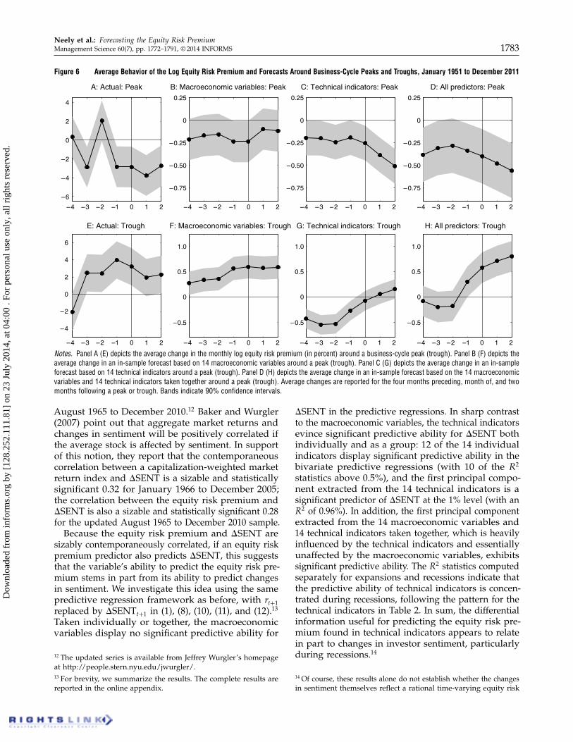
Figure 6 presents OLS estimates of the slope coef-ficients in (13) and (14), along with 90% confidenceintervals. Panel A of Figure 6 indicates that the actualequity risk premium declines significantly on averagefor most of the months around a cyclical peak, with anaverage decline of nearly 400 basis points for somemonths. Panel B shows that the expected equity riskpremium for the PC-ECON model only experiences

a significant decline for a few of the months arounda peak. In contrast, the PC-TECH model’s expectedequity risk premium in panel C falls significantly forall of the months near a peak, better matching thedepressed actual equity risk premium. Similarly to thePC-TECH model, panel D shows that the expectedequity risk premium for the PC-ALL model also fallssignificantly for most of the months around a peak.In addition, the coefficient magnitudes are larger forthe PC-ALL model in panel D relative to those for thePC-ECON and PC-TECH models in panels B and C,respectively, so that the PC-ALL model better capturesthe typically depressed actual equity risk premiumnear a peak.

Panel E of Figure 6 demonstrates that in contrast to acyclical peak, the actual equity risk premium typicallyrises significantly on average several months prior to acyclical trough. Generally in line with this behavior,the expected equity risk premium for the PC-ECONmodel in panel F increases significantly during themonths around a trough. The expected equity riskpremium for the PC-TECH model in panel G risesaround a trough, but the increase is not significant.The PC-ALL model’s average expected equity riskpremium increases significantly for many of the monthsaround a trough, and the increase in the expectedequity risk premium is large during and after a trough,

Dow

nloa

ded

from

info

rms.

org

by [

128.

252.

111.

81]

on 2

3 Ju

ly 2

014,

at 0

4:00

. Fo

r pe

rson

al u

se o

nly,

all

righ

ts r

eser

ved.


Figure 5 In-Sample Log Equity Risk Premium Forecasts Based on 14 Macroeconomic Variables and 14 Technical Indicators,January 1951 to December 2011

1955 1960 1965 1970 1975 1980 1985 1990 1995 2000 2005 2010

A: Principal component forecast based on macroeconomic variables

1955 1960 1965 1970 1975 1980 1985 1990 1995 2000 2005 2010

B: Principal component forecast based on technical indicators

1955 1960 1965 1970 1975 1980 1985 1990 1995 2000 2005 2010

0

–1

1

2

3

0

–1

1

2

3

0

–1

1

2

3

C: Principal component forecast based on macroeconomic variables and technical indicators taken together

Notes. Black lines delineate monthly log equity risk premium forecasts (in percent); gray lines delineate the average log equity risk premium over the sample.Panel A (B) depicts the forecast for a predictive regression model with a constant and the first three principal components extracted from 14 macroeconomicvariables (first principal component extracted from 14 technical indicators) serving as regressors. Panel C depicts the forecast for a predictive regression modelwith a constant and the first four principal components extracted from the 14 macroeconomic variables and 14 technical indicators taken together serving asregressors. Vertical bars depict NBER-dated recessions.

again helping the PC-ALL model to better matchthe rise in the actual equity risk premium around atrough.

Overall, Figure 6 indicates that the information intechnical indicators is more useful than that in macro-economic variables for detecting the typical decline inthe equity risk premium around a business-cycle peak,whereas macroeconomic variables provide more usefulinformation than technical indicators for ascertainingthe typical rise in the equity risk premium near acyclical trough. By incorporating information from bothmacroeconomic variables and technical indicators, thePC-TECH model exploits the information in each setof predictors to produce an expected equity risk pre-mium that better tracks the substantial countercyclicalfluctuations in the equity risk premium.

2.4. Sentiment and Conditional Asset PricingSections 2.1 and 2.2 show that technical indicatorspredict the equity risk premium. To further establishthat technical indicators contain meaningful economicinformation, we ask two questions.11 First, do technicalindicators forecast changes in investor sentiment, which

11 We thank the anonymous referees for suggesting these two inter-esting ideas.

are known to be correlated with stock returns? Second,do technical indicators have significant effects in aconditional asset pricing model? Positive answersto these questions provide further evidence of theeconomic relevance of technical indicators.

Positive answers to these questions also allay data-mining concerns, which are relevant for stock returnpredictability (e.g., Ferson et al. 2003). In particular,exploring the economic relevance of technical indicatorsalong additional dimensions reduces the likelihood thatthe significant predictive ability of technical indicatorsis a spurious result of excessively searching amongmeaningless predictors. Our out-of-sample tests in §3,including a modified version of the White (2000) realitycheck, also address data-mining concerns.

We answer the first question using the monthlysentiment-changes index from Baker and Wurgler(2007). This index (ãSENT) is the first principalcomponent extracted from changes in six sentimentproxies from Baker and Wurgler (2006): trading volume(measured by NYSE turnover), dividend premium(average market-to-book ratios of dividend paying andnonpaying firms), closed-end fund discount, initialpublic offering (IPO) number, IPO first-day returns,and equity share of total equity and debt issues byall corporations. We use an updated ãSENT series for

Dow

nloa

ded

from

info

rms.

org

by [

128.

252.

111.

81]

on 2

3 Ju

ly 2

014,

at 0

4:00

. Fo

r pe

rson

al u

se o

nly,

all

righ

ts r

eser

ved.


Figure 6 Average Behavior of the Log Equity Risk Premium and Forecasts Around Business-Cycle Peaks and Troughs, January 1951 to December 2011

0

2

4

A: Actual: Peak

0

0.25

–0.25

–0.50

–0.75

0

0.25

–0.25

–0.50

–0.75

0

0.25

–0.25

–0.50

–0.75

B: Macroeconomic variables: Peak C: Technical indicators: Peak D: All predictors: Peak

0–1–2

–2

–3–4

–4

1 2 0–1–2–3–4

–0.5

1 2 0–1–2–3–4 1 2 0–1–2–3–4 1 2

0–1–2–3–4

–6

–4

–2

1 2 0–1–2–3–4 1 2 0–1–2–3–4 1 2 0–1–2–3–4 1 2

0

2

4

6

E: Actual: Trough

0

0.5

1.0

–0.5

0

0.5

1.0

–0.5

0

0.5

1.0

F: Macroeconomic variables: Trough G: Technical indicators: Trough H: All predictors: Trough

Notes. Panel A (E) depicts the average change in the monthly log equity risk premium (in percent) around a business-cycle peak (trough). Panel B (F) depicts theaverage change in an in-sample forecast based on 14 macroeconomic variables around a peak (trough). Panel C (G) depicts the average change in an in-sampleforecast based on 14 technical indicators around a peak (trough). Panel D (H) depicts the average change in an in-sample forecast based on the 14 macroeconomicvariables and 14 technical indicators taken together around a peak (trough). Average changes are reported for the four months preceding, month of, and twomonths following a peak or trough. Bands indicate 90% confidence intervals.

August 1965 to December 2010.12 Baker and Wurgler(2007) point out that aggregate market returns andchanges in sentiment will be positively correlated ifthe average stock is affected by sentiment. In supportof this notion, they report that the contemporaneouscorrelation between a capitalization-weighted marketreturn index and ãSENT is a sizable and statisticallysignificant 0.32 for January 1966 to December 2005;the correlation between the equity risk premium andãSENT is also a sizable and statistically significant 0.28for the updated August 1965 to December 2010 sample.

Because the equity risk premium and ãSENT aresizably contemporaneously correlated, if an equity riskpremium predictor also predicts ãSENT, this suggeststhat the variable’s ability to predict the equity risk pre-mium stems in part from its ability to predict changesin sentiment. We investigate this idea using the samepredictive regression framework as before, with rt+1replaced by ãSENTt+1 in (1), (8), (10), (11), and (12).13

Taken individually or together, the macroeconomicvariables display no significant predictive ability for

12 The updated series is available from Jeffrey Wurgler’s homepageat http://people.stern.nyu.edu/jwurgler/.13 For brevity, we summarize the results. The complete results arereported in the online appendix.

ãSENT in the predictive regressions. In sharp contrastto the macroeconomic variables, the technical indicatorsevince significant predictive ability for ãSENT bothindividually and as a group: 12 of the 14 individualindicators display significant predictive ability in thebivariate predictive regressions (with 10 of the R2

statistics above 0.5%), and the first principal compo-nent extracted from the 14 technical indicators is asignificant predictor of ãSENT at the 1% level (with anR2 of 0.96%). In addition, the first principal componentextracted from the 14 macroeconomic variables and14 technical indicators taken together, which is heavilyinfluenced by the technical indicators and essentiallyunaffected by the macroeconomic variables, exhibitssignificant predictive ability. The R2 statistics computedseparately for expansions and recessions indicate thatthe predictive ability of technical indicators is concen-trated during recessions, following the pattern for thetechnical indicators in Table 2. In sum, the differentialinformation useful for predicting the equity risk pre-mium found in technical indicators appears to relatein part to changes in investor sentiment, particularlyduring recessions.14

14 Of course, these results alone do not establish whether the changesin sentiment themselves reflect a rational time-varying equity risk

Dow

nloa

ded

from

info

rms.

org

by [

128.

252.

111.

81]

on 2

3 Ju

ly 2

014,

at 0

4:00

. Fo

r pe

rson

al u

se o

nly,

all

righ

ts r

eser

ved.


Turning to the second question, in the spirit of Fersonand Harvey (1999), we estimate a conditional versionof the Fama and French (1993) three-factor model:

Ri1 t+1 −Rf 1 t+1 = �i1 t +�MKTi1 t MKTt+1 +�SMB

i1 t SMBt+1

+�HMLi1 t HMLt+1 + �i1 t+11 (15)

where Ri1 t+1 is the (simple) return on portfolio i, Rf isthe risk-free return, MKT is the excess market return,SMB (HML) is the size (value) premium, and

�i1 t = �i10 +

4∑

k=1

�i1 kF̂ALLk1 t 1 (16)

�ji1 t = �

ji10 +

4∑

k=1

�j

i1 kF̂ALLk1 t

for j = MKT1 SMB1 HML0 (17)

Equation (15) is a conditional asset pricing model inthat it permits time variation in both “alpha” via (16)and the factor exposures via (17). We estimate (15)for 10 momentum-sorted portfolios, as well as the“up-minus-down” (UMD) zero-investment momentumportfolio, using data from Kenneth French’s DataLibrary.15 Momentum portfolios present challenges forthe unconditional Fama–French three-factor model (e.g.,Fama and French 1996, Carhart 1997), and we examinewhether the information in lagged macroeconomicvariables and technical indicators, as captured by F̂ ALL

k1 t

(j = 11 0 0 0 14), enters significantly into a conditionalversion of the model.

For each of the 11 momentum portfolios, we firsttest the joint null hypothesis,

�i11 = �MKTi11 = �SMB

i11 = �HMLi11 = 00 (18)

Because F̂ ALL11 t corresponds closely to the technical indi-

cators, (18) essentially tests the significance of thetechnical indicators as a group in the conditional assetpricing model. Using heteroskedasticity-robust �2-statistics, we reject the restrictions in (18) for 10 ofthe 11 momentum portfolios.16 Technical indicatorsthus significantly explain returns in the conditionalasset pricing model given by (15) for nearly all portfo-lios, which provides additional evidence that technicalindicators represent genuine economic information.

We next test the joint null hypothesis,

�i1 k = �MKTi1 k = �SMB

i1 k = �HMLi1 k = 0 for k = 213140 (19)

premium or irrational fluctuations in investor sentiment (or both).Determining the sources of the changes in investor sentiment requiresa full-fledged model of equilibrium returns, which is beyond thescope of the present paper.15 The data are available at http://mba.tuck.dartmouth.edu/pages/faculty/ken.french/data_library.html.16 The complete set of �2-statistics is reported in the online appendix.

Because F̂ ALL21 t , F̂ ALL

31 t , and F̂ ALL41 t correspond closely to the

macroeconomic variables, (19) tests the significanceof the macroeconomic variables as a group. We rejectthe restrictions in (19) for all 11 momentum portfolios;like technical indicators, macroeconomic variablessignificantly explain portfolio returns in the conditionalasset pricing model. We also test the null,

�i1k =�MKTi1k =�SMB

i1k =�HMLi1k =0 for k=11213141 (20)

which tests the significance of the technical indica-tors and macroeconomic variables taken together. Wealso reject the restrictions in (20) for all 11 portfolios.In accord with our predictive regression results, wethus find that macroeconomic variables and technicalindicators both enter significantly in the conditionalFama–French three-factor model.17

3. Out-of-Sample AnalysisAs a robustness check, this section reports out-of-sample forecasting statistics for the 14 macroeconomicvariables and 14 technical indicators. The month-(t + 1)out-of-sample equity risk premium forecast based onan individual macroeconomic variable in (1) and datathrough month t is given by

r̂t+1 = �̂t1 i + �̂t1 ixi1 t1 (21)

where �̂t1 i and �̂t1 i are the OLS estimates from regress-ing 8rs9

ts=2 on a constant and 8xi1 s9

t−1s=1. We use December

1950 to December 1965 as the initial estimation period,so that the forecast evaluation period spans fromJanuary 1966 to December 2011 (552 observations).The length of the initial in-sample estimation periodbalances having enough observations for reasonablyprecisely estimating the initial parameters with ourdesire for a relatively long out-of-sample period forforecast evaluation.18

The out-of-sample forecast based on an individualtechnical indicator in (8) is given by

r̂t+1 = �̂t1 i + �̂t1 iSi1 t1 (22)

where �̂t1 i and �̂t1 i are the OLS estimates from regress-ing 8rs9

ts=2 on a constant and 8Si1 s9

t−1s=1. We also generate

17 We also estimated a conditional version of the Fama–French three-factor model that does not permit time variation in the alphas, sothat �i1 t = �i10 in (16). The qualitative results are unchanged for testsof relevant versions of (18), (19), and (20).18 Hansen and Timmermann (2012) show that out-of-sample testsof predictive ability have better size properties when the forecastevaluation period is a relatively large proportion of the availablesample, as in our case.

Dow

nloa

ded

from

info

rms.

org

by [

128.

252.

111.

81]

on 2

3 Ju

ly 2

014,

at 0

4:00

. Fo

r pe

rson

al u

se o

nly,

all

righ

ts r

eser

ved.


out-of-sample forecasts based on principal components,as in (10), (11), and (12):

r̂jt+1 = �̂t +

K∑

k=1

�̂t1 kF̂j

12 t1 k1 t

for j = ECON, TECH, or ALL1 (23)

where F̂j

12 t1 k1 t is the kth principal component extractedfrom the 14 macroeconomic variables (j = ECON),14 technical indicators (j = TECH), or 14 macroeco-nomic variables and 14 technical indicators takentogether (j = ALL), based on data through t; and �̂t and�̂t1 k (k = 11 0 0 0 1K) are the OLS estimates from regress-ing 8rs9

ts=2 on a constant and 8F̂

j

12 t1 k1 s9t−1s=1 (k = 11 0 0 0 1K).19

We compare the forecasts given by (21), (22), and(23) to the historical average forecast:

r̂HAt+1 = 41/t5

t∑

s=1

rs0 (24)

This popular benchmark forecast (e.g., Goyal and Welch2003, 2008; Campbell and Thompson 2008; Ferreira andSanta-Clara 2011) assumes a constant expected equityrisk premium (rt+1 = �+ �t+1). Goyal and Welch (2003,2008) show that (24) is a very stringent out-of-samplebenchmark: predictive regression forecasts based onindividual macroeconomic variables typically fail tooutperform the historical average.

We analyze forecasts in terms of the Campbell andThompson (2008) out-of-sample R2 (R2

OS) and Clark andWest (2007) MSFE-adjusted statistics. The R2

OS statisticmeasures the proportional reduction in mean squaredforecast error (MSFE) for the predictive regressionforecast relative to the historical average. A positivevalue thus indicates that the predictive regressionforecast outperforms the historical average in termsof MSFE, whereas a negative value signals the oppo-site. Like their in-sample counterparts, monthly R2

OS

statistics appear small at first glance because of theinherently large unpredictable component in stockreturns; nevertheless, a monthly R2

OS statistic near 0.5%is economically significant (Campbell and Thompson2008). The MSFE-adjusted statistic tests the null hypoth-esis that the historical average MSFE is less than orequal to the predictive regression MSFE against theone-sided (upper-tail) alternative hypothesis that thehistorical average MSFE is greater than the predictiveregression MSFE (corresponding to H0: R2

OS ≤ 0 againstHA: R2

OS > 0).20

19 We select K via the adjusted R2 based on data through t.20 Clark and West (2007) develop the MSFE-adjusted statistic bymodifying the familiar Diebold and Mariano (1995) and West(1996) statistic so that it has an approximately standard normalasymptotic distribution when comparing forecasts from nestedmodels. Comparing a predictive regression forecast to the historicalaverage entails comparing nested models, because the predictiveregression model reduces to the constant expected equity riskpremium model under the null hypothesis.

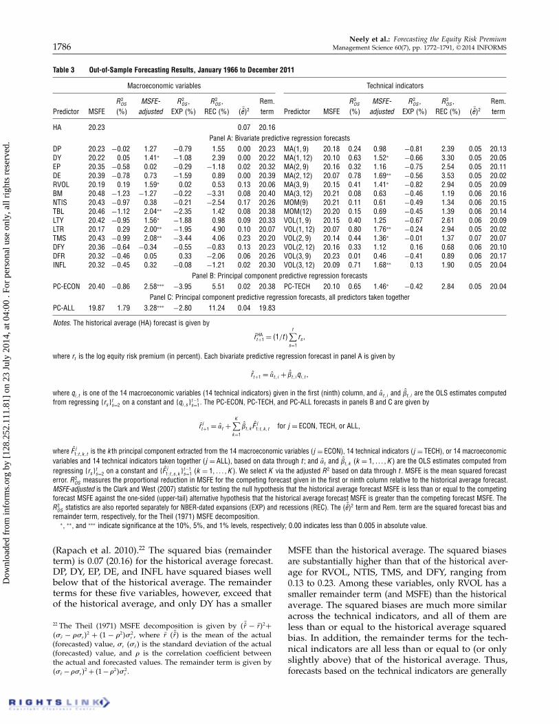
Panel A of Table 3 reports out-of-sample resultsfor bivariate predictive regression forecasts based onindividual macroeconomic variables and technicalindicators. Only three of the R2

OS statistics are positivein the third column of panel A; the vast majorityof individual macroeconomic variables thus fail tooutperform the historical average benchmark in termsof MSFE. The three positive R2

OS statistics (for DY,RVOL, and LTR) only range from 0.05% to 0.29%.Nevertheless, the MSFEs for these three predictors aresignificantly less than the historical average MSFE atconventional levels according to the MSFE-adjustedstatistics in the fourth column. It is interesting to notethat the MSFE-adjusted statistics indicate that the MSFEsfor TBL, LTY, and TMS are significantly less thanthat of the historical average, despite the negativeR2

OS statistics for these forecasts. Although this resultappears strange, it is possible when comparing nestedmodel forecasts (Clark and West 2007, McCracken2007).21 Reminiscent of Goyal and Welch (2003, 2008),individual macroeconomic variables display limitedout-of-sample predictive ability in Table 3, panel A.Similarly to the in-sample results in Table 2, a numberof macroeconomic variables—including DP, DY, TBL,LTR, and TMS—predict the equity risk premium betterduring recessions than expansions on an out-of-samplebasis.

Overall, individual technical indicators appear toperform as well as, or better than, individual macro-economic variables in terms of MSFE. All of the R2

OS

statistics are positive in the eleventh column of Table 3,panel A; each of the technical indicators thus deliversa lower MSFE than the historical average benchmark.Three of the R2

OS statistics exceed 0.70%, and the MSFEsfor six of the technical indicators are significantlyless than the historical average MSFE based on theMSFE-adjusted statistics. Again matching the in-sampleresults, the out-of-sample predictive ability of technicalindicators is uniformly stronger for recessions relativeto expansions.

To get a sense of potential bias-efficiency trade-offsin the forecasts, Table 3 also reports the Theil (1971)MSFE decomposition into the squared forecast bias anda remainder term. The remainder term depends, amongother things, on the forecast volatility, and limitingforecast volatility helps to reduce the remainder term

21 Intuitively, under the null hypothesis that the constant expectedequity risk premium model generates the data, the predictiveregression model produces a noisier forecast than does the historicalaverage benchmark because it estimates slope parameters with zeropopulation values. We thus expect the benchmark model MSFE tobe smaller than the predictive regression model MSFE under thenull. The MSFE-adjusted statistic accounts for the negative expecteddifference between the historical average MSFE and predictiveregression MSFE under the null, so that it can reject the null even ifthe R2

OS statistic is negative.

Dow

nloa

ded

from

info

rms.

org

by [

128.

252.

111.

81]

on 2

3 Ju

ly 2

014,

at 0

4:00

. Fo

r pe

rson

al u

se o

nly,

all

righ

ts r

eser

ved.


Table 3 Out-of-Sample Forecasting Results, January 1966 to December 2011


R2OS MSFE- R2

OS , R2OS , Rem. R2

OS MSFE- R2OS , R2

OS , Rem.Predictor MSFE (%) adjusted EXP (%) REC (%) 4 ¯̂e52 term Predictor MSFE (%) adjusted EXP (%) REC (%) 4 ¯̂e52 term

HA 20.23 0.07 20.16Panel A: Bivariate predictive regression forecasts

DP 20.23 −0002 1027 −0079 1055 0.00 20.23 MA(1, 9) 20.18 0.24 0098 −0081 2.39 0.05 20.13DY 20.22 0005 1041∗ −1008 2039 0.00 20.22 MA(1, 12) 20.10 0.63 1052∗ −0066 3.30 0.05 20.05EP 20.35 −0058 0002 −0029 −1018 0.02 20.32 MA(2, 9) 20.16 0.32 1016 −0075 2.54 0.05 20.11DE 20.39 −0078 0073 −1059 0089 0.00 20.39 MA(2, 12) 20.07 0.78 1069∗∗ −0056 3.53 0.05 20.02RVOL 20.19 0019 1059∗ 0002 0053 0.13 20.06 MA(3, 9) 20.15 0.41 1041∗ −0082 2.94 0.05 20.09BM 20.48 −1023 −1027 −0022 −3031 0.08 20.40 MA(3, 12) 20.21 0.08 0063 −0046 1.19 0.06 20.16NTIS 20.43 −0097 0038 −0021 −2054 0.17 20.26 MOM(9) 20.21 0.11 0061 −0049 1.34 0.06 20.15TBL 20.46 −1012 2004∗∗ −2035 1042 0.08 20.38 MOM(12) 20.20 0.15 0069 −0045 1.39 0.06 20.14LTY 20.42 −0095 1056∗ −1088 0098 0.09 20.33 VOL(1, 9) 20.15 0.40 1025 −0067 2.61 0.06 20.09LTR 20.17 0029 2000∗∗ −1095 4090 0.10 20.07 VOL(1, 12) 20.07 0.80 1076∗∗ −0024 2.94 0.05 20.02TMS 20.43 −0099 2008∗∗ −3044 4006 0.23 20.20 VOL(2, 9) 20.14 0.44 1036∗ −0001 1.37 0.07 20.07DFY 20.36 −0064 −0034 −0055 −0083 0.13 20.23 VOL(2, 12) 20.16 0.33 1012 0016 0.68 0.06 20.10DFR 20.32 −0046 0005 0033 −2006 0.06 20.26 VOL(3, 9) 20.23 0.01 0046 −0041 0.89 0.06 20.17INFL 20.32 −0045 0032 −0008 −1021 0.02 20.30 VOL(3, 12) 20.09 0.71 1068∗∗ 0013 1.90 0.05 20.04

Panel B: Principal component predictive regression forecastsPC-ECON 20.40 −0086 2058∗∗∗ −3095 5051 0.02 20.38 PC-TECH 20.10 0.65 1046∗ −0042 2.84 0.05 20.04

Panel C: Principal component predictive regression forecasts, all predictors taken togetherPC-ALL 19.87 1079 3028∗∗∗ −2080 11024 0.04 19.83

Notes. The historical average (HA) forecast is given by

r̂ HAt+1 = 41/t5

t∑

s=1

rs1

where rt is the log equity risk premium (in percent). Each bivariate predictive regression forecast in panel A is given by

r̂t+1 = �̂t1 i + �̂t1 iqi1 t 1

where qi1 t is one of the 14 macroeconomic variables (14 technical indicators) given in the first (ninth) column, and �̂t1 i and �̂t1 i are the OLS estimates computedfrom regressing 8rs9

ts=2 on a constant and 8qi1 s9

t−1s=1. The PC-ECON, PC-TECH, and PC-ALL forecasts in panels B and C are given by

r̂ jt+1 = �̂t +

K∑

k=1

�̂t1 k F̂j

12 t1 k1 t for j = ECON, TECH, or ALL1

where F̂ j12 t1 k1 t is the kth principal component extracted from the 14 macroeconomic variables (j = ECON), 14 technical indicators (j = TECH), or 14 macroeconomic

variables and 14 technical indicators taken together (j = ALL), based on data through t ; and �̂t and �̂t1 k (k = 11 0 0 0 1 K ) are the OLS estimates computed fromregressing 8rs9

ts=2 on a constant and 8F̂ j

12 t1 s1 k9t−1s=1 (k = 11 0 0 0 1 K ). We select K via the adjusted R2 based on data through t . MSFE is the mean squared forecast

error. R2OS measures the proportional reduction in MSFE for the competing forecast given in the first or ninth column relative to the historical average forecast.

MSFE-adjusted is the Clark and West (2007) statistic for testing the null hypothesis that the historical average forecast MSFE is less than or equal to the competingforecast MSFE against the one-sided (upper-tail) alternative hypothesis that the historical average forecast MSFE is greater than the competing forecast MSFE. TheR2OS statistics are also reported separately for NBER-dated expansions (EXP) and recessions (REC). The 4 ¯̂e52 term and Rem. term are the squared forecast bias and

remainder term, respectively, for the Theil (1971) MSFE decomposition.∗, ∗∗, and ∗∗∗ indicate significance at the 10%, 5%, and 1% levels, respectively; 0.00 indicates less than 0.005 in absolute value.

(Rapach et al. 2010).22 The squared bias (remainderterm) is 0.07 (20.16) for the historical average forecast.DP, DY, EP, DE, and INFL have squared biases wellbelow that of the historical average. The remainderterms for these five variables, however, exceed thatof the historical average, and only DY has a smaller

22 The Theil (1971) MSFE decomposition is given by 4 ¯̂r − r̄ 52+

4�r̂ − ��r 52 + 41 − �25� 2

r , where r̄ ( ¯̂r) is the mean of the actual(forecasted) value, �r (�r̂ ) is the standard deviation of the actual(forecasted) value, and � is the correlation coefficient betweenthe actual and forecasted values. The remainder term is given by4�r̂ −��r 5

2 + 41 −�25� 2r .

MSFE than the historical average. The squared biasesare substantially higher than that of the historical aver-age for RVOL, NTIS, TMS, and DFY, ranging from0.13 to 0.23. Among these variables, only RVOL has asmaller remainder term (and MSFE) than the historicalaverage. The squared biases are much more similaracross the technical indicators, and all of them areless than or equal to the historical average squaredbias. In addition, the remainder terms for the tech-nical indicators are all less than or equal to (or onlyslightly above) that of the historical average. Thus,forecasts based on the technical indicators are generally

Dow

nloa

ded

from

info

rms.

org

by [

128.

252.

111.

81]

on 2

3 Ju

ly 2

014,

at 0

4:00

. Fo

r pe

rson

al u

se o

nly,

all

righ

ts r

eser

ved.


both less biased and more efficient than the historicalaverage.

Panel B of Table 3 reports out-of-sample results forthe principal component predictive regression forecastsbased on macroeconomic variables or technical indica-tors. Although the R2

OS is negative for the PC-ECONforecast, its MSFE is significantly less (at the 1% level)than that of the historical average according to theMSFE-adjusted statistic.23 The R2

OS is 0.65% for the PC-TECH forecast, and the MSFE-adjusted statistic indicatesthat the MSFE for the PC-TECH forecast is significantlybelow that of the historical average. The PC-ECON andPC-TECH forecasts have smaller squared biases thandoes the historical average. The remainder term for thePC-ECON forecast, however, substantially exceeds thatof the historical average; in contrast, the remainderterm for the PC-TECH forecast is well below that ofthe historical average. Both the PC-ECON and PC-TECH forecasts manifest much stronger out-of-samplepredictive ability in recessions than in expansions.

We next compare the information content of thePC-ECON and PC-TECH forecasts using encompassingtests. Harvey et al. (1998) develop a statistic for test-ing the null hypothesis that a given forecast containsall of the relevant information found in a compet-ing forecast (i.e., the given forecast encompasses thecompetitor) against the alternative that the competingforecast contains relevant information beyond thatin the given forecast. We reject the null hypothesisthat the PC-ECON forecast encompasses the PC-TECHforecast as well as the null that the PC-TECH forecastencompasses the PC-ECON forecast (both at the 1%level; the complete results are omitted for brevity).The PC-ECON and PC-TECH forecasts thus fail toencompass each other, indicating that there are gainsto using information from macroeconomic variablesand technical indicators in conjunction.

In accord with the encompassing test results, the PC-ALL forecast has an R2

OS of 1.79% in Table 3, panel C,which easily exceeds all of the other R2

OS statisticsin Table 3. The PC-ALL MSFE is also significantlyless than the historical average MSFE at the 1% levelaccording to the MSFE-adjusted statistic. The squaredbias and remainder term for the PC-ALL forecast areboth below the respective values for the historicalaverage; indeed, the remainder term for the PC-ALLforecast is well below that of any of the other forecasts.The out-of-sample results in Table 3 thus confirmthe in-sample results in §2: macroeconomic variablesand technical indicators capture different types ofinformation relevant for forecasting the equity risk

23 See Footnote 21 for the intuition behind this seemingly strangeresult.

premium.24 The R2OS for the PC-ALL forecast is a very

sizable 11.24% for recessions, whereas it is −2080%for expansions, so that the out-of-sample predictivepower of the macroeconomic variables and technicalindicators taken together is highly concentrated inrecessions.

To control for data mining—which becomes a con-cern when considering many predictors—we use theClark and McCracken (2012) modified version of theWhite (2000) reality check. The Clark and McCracken(2012) reality check is based on a wild fixed-regressorbootstrap and is appropriate for comparing forecastsfrom multiple models, all of which nest the benchmarkmodel, as in our framework. We use the Clark andMcCracken (2012) maxMSFE-F statistic to test the nullhypothesis that the historical average MSFE is less thanor equal to the minimum MSFE of all the 28 bivariatepredictive regression forecasts and three principal com-ponent predictive regression forecasts in Table 3. ThemaxMSFE-F statistic rejects the null that none of thecompeting forecasts outperforms the historical average,with a bootstrapped p-value of 0.03, so that data miningcannot readily explain the significant out-of-samplepredictive power of the PC-ALL forecast.25

4. Asset Allocation ExerciseAs a final exercise, we measure the economic value ofequity risk premium forecasts for a risk-averse investor.Following Campbell and Thompson (2008) and Ferreiraand Santa-Clara (2011), among others, we computethe certainty equivalent return (CER) for an investorwith mean-variance preferences who monthly allocatesacross equities and risk-free bills using various equityrisk premium forecasts. This exercise also addressesthe weakness of many existing studies of technicalindicators that fail to incorporate risk aversion into theasset allocation decision.

24 The PC-ALL forecast also has a lower MSFE than the constant0.5% equity risk premium benchmark forecast used by Simin (2008).Rapach et al. (2010) show that a combination forecast of the equityrisk premium based on individual predictive regressions withmacroeconomic variables delivers consistent out-of-sample gains.Using the same approach, we form a combination forecast as themean of the 14 bivariate predictive regression forecasts in Table 3,panel A, and its R2

OS is 1.16%. Ferreira and Santa-Clara (2011) proposean intriguing “sum-of-the-parts” equity risk premium forecast asthe sum of a 20-year moving average of earnings growth and thecurrent dividend-price ratio (minus the risk-free rate). We compute asum-of-the-parts forecast, and its R2

OS is 1.32%. The PC-ALL forecastthus appears to be the best-to-date out-of-sample forecast of theequity risk premium.25 Ferson et al. (2003) demonstrate that size distortions related tothe Stambaugh bias can exacerbate data-mining problems for in-sample predictive regressions with persistent predictors. Busettiand Marcucci (2012), however, show that out-of-sample tests ofpredictive ability are not afflicted by size distortions in the presenceof persistent predictors, so the issues raised by Ferson et al. (2003)do not appear of great concern for our out-of-sample analysis.

Dow

nloa

ded

from

info

rms.

org

by [

128.

252.

111.

81]

on 2

3 Ju

ly 2

014,

at 0

4:00

. Fo

r pe

rson

al u

se o

nly,

all

righ

ts r

eser

ved.


At the end of month t, the investor optimally allocatesthe following share of the portfolio to equities duringmonth t + 1:

wt =

(

1�

)(

r̂t+1

�̂2t+1

)

1 (25)

where r̂t+1 is a forecast of the (simple) equity riskpremium and �̂2

t+1 is a forecast of its variance. Theshare 1 − wt is allocated to risk-free bills, and themonth-(t + 1) portfolio return is given by

Rp1 t+1 =wtrt+1 +Rf 1 t+10 (26)

Following Campbell and Thompson (2008), we assumethat the investor uses a five-year moving window ofpast monthly returns to estimate the variance of theequity risk premium and constrain wt to lie between 0and 1.5.26

The CER for the portfolio is

CERp = �̂p −12��̂

2p 1 (27)

where �̂p and �̂2p are the mean and variance, respec-

tively, for the investor’s portfolio over the forecastevaluation period. The CER can be interpreted as therisk-free rate of return that an investor is willing toaccept instead of adopting the given risky portfolio.The CER gain is the difference between the CER for theinvestor who uses a predictive regression forecast ofthe equity risk premium based on (21), (22), or (23) andthe CER for an investor who uses the historical averageforecast given by (24). We multiply this differenceby 1,200, so that it can be interpreted as the annualpercentage portfolio management fee that an investorwould be willing to pay to have access to the predictiveregression forecast instead of the historical averageforecast.

The second and ninth columns of panel A in Table 4present CER gains for an investor with a relativerisk coefficient of five who relies on the bivariatepredictive regression forecast given by (21) or (22),respectively, instead of the historical average forecast;for the historical average forecast, the table reports theCER level. Table 4 also reports additional portfolioperformance measures. The monthly Sharpe ratio inthe fifth and twelfth columns is the mean portfolioreturn in excess of the risk-free rate divided by thestandard deviation of the excess portfolio return. Thesixth and thirteenth columns report average monthlyturnover, where monthly turnover is the percentageof wealth traded each month. For the portfolio basedon the historical average forecast, the table gives theaverage monthly turnover; for the other portfolios, itgives the relative average turnover (average monthlyturnover divided by the average monthly turnover for

26 This imposes realistic portfolio constraints by precluding shortsales and preventing more than 50% leverage.

the portfolio based on the historical average forecast).The seventh and final columns report CER gains netof transactions costs, where the costs are calculatedusing the monthly turnover measures and assuming aproportional transactions cost equal to 50 basis pointsper transaction (Balduzzi and Lynch 1999).

Table 4 reports that the CER for the portfolio based onthe historical average forecast is 3.54% for January 1966to December 2011. The CER gains are positive for 9 ofthe 14 macroeconomic variables in the second columnof Table 4, panel A, with TBL, LTY, LTR, and TMSproviding gains of more than 100 basis points. In accordwith the R2

OS statistics in Table 3, the CER gains aresubstantially larger for recessions vis-à-vis expansionsfor many of the macroeconomic variables. Eight of themacroeconomic predictors produce higher monthlySharpe ratios than that of the historical average, withTMS generating the highest ratio of 0.12. The averageturnover is 2.09% for the historical average. Portfoliosbased on many of the macroeconomic variables turnover approximately three to five times more often thanthe historical average portfolio, and the LTR portfolioturns over nearly 24 times as much. After accountingfor transactions costs, the relatively high turnovers forNTIS, LTR, DFR, and INFL reduce the CER gains frompositive to negative values.

The last six columns of panel A in Table 4 revealthat portfolios based on technical indicators generallyoutperform those based on macroeconomic variables.The CER gains in the ninth column are positive forall of the technical indicators, reaching a maximumof 317 basis points. Again in accord with the R2

OS

statistics, the CER gains are uniformly larger duringrecessions relative to expansions, and the gains forrecessions are greater than 1,000 basis points for 10 ofthe 14 individual technical indicators. Portfolios basedon the technical indicators turn over approximatelytwo to five times more often than the historical averageportfolio. Despite this turnover, the net-of-transactions-costs CER gains are positive—and as high as 282 basispoints—for all of the technical indicators.

Panels B and C of Table 4 report performance mea-sures for portfolios based on the principal componentpredictive regression forecasts given by (23). PC-ECONdelivers a sizable CER gain of 224 basis points in thesecond column of panel B, and its monthly Sharperatio of 0.10 is twice that of the historical average.The CER gain for PC-ECON is much larger for reces-sions (1,269 basis points) compared to expansions(9 basis points). Although the PC-ECON portfolioturns over nearly seven times more often than thehistorical average portfolio, it still improves the net-of-transactions-costs CER by 151 basis points. PC-TECHgenerates a CER gain of 249 basis points in the ninthcolumn of panel B, 25 basis points more than PC-ECON,and a monthly Sharpe ratio of 0.10, matching that

Dow

nloa

ded

from

info

rms.

org

by [

128.

252.

111.

81]

on 2

3 Ju

ly 2

014,

at 0

4:00

. Fo

r pe

rson

al u

se o

nly,

all

righ

ts r

eser

ved.


Table 4 Portfolio Performance Measures, January 1966 to December 2011


Relative ã (ann.), Relative ã (ann.),ã (ann.) ã (ann.), ã (ann.), Sharpe average cost = ã (ann.) ã (ann.), ã (ann.), Sharpe average cost =

Predictor (%) EXP (%) REC (%) ratio turnover 50 bps (%) Predictor (%) EXP (%) EXP (%) ratio turnover 50 bps (%)

HA 3054 0.05 2009% 3040Panel A: Bivariate predictive regression forecasts

DP −0026 −0098 2094 0.03 2017 −0038 MA(1, 9) 1.69 −0051 12069 0.08 4.40 1.22DY 0027 −1013 6089 0.04 3005 0002 MA(1, 12) 2.91 −0027 18091 0.11 3.94 2.51EP 0042 −0001 2043 0.05 1072 0034 MA(2, 9) 2.08 −0049 14008 0.09 4.48 1.63DE −0019 −1026 4099 0.04 2017 −0034 MA(2, 12) 3.17 −0007 19017 0.12 3.62 2.82RVOL −0052 −0011 −2097 0.08 4020 −0090 MA(3, 9) 2.54 −0037 17054 0.11 4.60 2.08BM −1026 −0016 −6069 0.03 2052 −1045 MA(3, 12) 1.40 −0039 10040 0.08 2.69 1.18NTIS 0015 0065 −2030 0.08 3052 −0018 MOM(9) 1.38 −0041 10038 0.07 2.58 1.16TBL 1062 0076 5081 0.08 1052 1056 MOM(12) 1.32 −0040 9032 0.07 2.19 1.16LTY 1065 0048 7040 0.07 1003 1065 VOL(1, 9) 1.61 −0072 13061 0.08 5.21 1.05LTR 1007 −0063 9017 0.09 23094 −1087 VOL(1, 12) 2.63 −0026 17063 0.11 4.59 2.25TMS 1088 0042 8095 0.12 4045 1044 VOL(2, 9) 1.48 −0007 9048 0.08 2.94 1.23DFY −0082 −0019 −4001 0.05 2070 −1003 VOL(2, 12) 1.32 0010 7032 0.08 2.40 1.13DFR 0026 0066 −1068 0.06 10016 −0091 VOL(3, 9) 0.71 −0042 6071 0.06 2.52 0.52INFL 0038 0003 2013 0.06 7077 −0049 VOL(3, 12) 2.22 −0005 13022 0.10 2.80 1.99

Panel B: Principal component predictive regression forecastsPC-ECON 2024 0009 12069 0.10 6073 1051 PC-TECH 2.49 −0029 16037 0.10 3.58 2.15

Panel C: Principal component predictive regression forecasts, all predictors taken togetherPC-ALL 4094 0070 26021 0.16 7051 4012

Notes. This table reports portfolio performance measures for an investor with mean-variance preferences and relative risk-aversion coefficient of five who monthlyallocates between equities and risk-free bills using either an historical average (HA) or predictive regression equity risk premium forecast. Each forecast in panel Ais based on one of the 14 macroeconomic variables (14 technical indicators) given in the first (eighth) column. The forecasts in panels B and C are based on the 14macroeconomic variables (PC-ECON), 14 technical indicators (PC-TECH), or all 14 macroeconomic variables and 14 technical indicators taken together (PC-ALL).The ã statistic is the annualized certainty equivalent return (CER) gain for an investor who uses the predictive regression forecast instead of the historical averageforecast; for the historical average forecast, the table reports the CER level; ã statistics are also reported separately for NBER-dated expansions (EXP) andrecessions (REC). Relative average turnover is the average turnover for the portfolio based on the predictive regression forecast divided by the average turnover forthe portfolio based on the historical average forecast; for the historical average forecast, the table reports the average turnover level. The ã, cost = 50 bps statisticis the CER gain assuming a proportional transactions cost of 50 basis points per transaction.

of PC-ECON. PC-TECH provides substantially largerCER gains for recessions (1,637 basis points) relative toexpansions (−29 basis points). Because the PC-TECHportfolio turns over much less than the PC-ECONportfolio, the net-of-transactions-costs CER gain forPC-TECH remains well above 200 basis points.

The performance of PC-ALL in panel C of Table 4stands out. The CER gain for PC-ALL in the secondcolumn of panel C is more than 170 basis points higherthan that of any of the other portfolios in Table 4.PC-ALL also produces the highest monthly Sharperatio, 0.16, and the highest net-of-transactions-costsCER gain, 412 basis points, of all the portfolios. TheCER gain accruing to PC-ALL reaches a very siz-able 2,621 basis points for recessions compared to70 basis points for expansions, again in line with theR2

OS statistics in Table 3. The asset allocation exercisedemonstrates the substantial economic value of com-bining information from macroeconomic variables andtechnical indicators.

5. ConclusionWe utilize technical indicators to directly forecast theequity risk premium and compare their performance

with that of macroeconomic variables. Our resultsshow that technical indicators exhibit statistically andeconomically significant in-sample and out-of-samplepredictive power for the monthly equity risk premium,clearly on par with that of well-known macroeconomicvariables from the literature. Furthermore, we findthat technical indicators and macroeconomic variablescapture different types of information relevant for fore-casting the equity risk premium; in particular, technicalindicators (macroeconomic variables) better detect thetypical decline (rise) in the equity risk premium nearbusiness-cycle peaks (troughs). In line with this finding,we demonstrate that combining information from bothtechnical indicators and macroeconomic variables pro-duces superior equity risk premium forecasts and offerssizable utility gains to investors by better tracking thesubstantial countercyclical fluctuations in the equityrisk premium.

Although numerous theories explain why technicalindicators may work (as reviewed in the introduction),little is known about their ability to explain key stylizedfacts concerning stock market returns, such as theequity risk premium puzzle (i.e., the average equityrisk premium appears too large in light of conventional

Dow

nloa

ded

from

info

rms.

org

by [

128.

252.

111.

81]

on 2

3 Ju

ly 2

014,

at 0

4:00

. Fo

r pe

rson

al u

se o

nly,

all

righ

ts r

eser

ved.


risk considerations). In contrast, more traditional assetpricing models, such as the habit model of Campbelland Cochrane (1999) and long-run risks model of Bansaland Yaron (2004), can explain important stylized facts,but they leave no role for technical analysis. Given thegrowing empirical evidence supporting the predictivepower of technical indicators, which is in line with thebehavior of many practitioners, it appears important tobridge the gap between theoretical models of technicalanalysis and more traditional asset pricing models.Exploring the connections between these two types ofmodels holds the promise of significantly improvingour understanding of the economic forces that drivethe equity risk premium and cross-section of expectedasset returns.

Supplemental MaterialSupplemental material to this paper is available at http://dx.doi.org/10.1287/mnsc.2013.1838.

AcknowledgmentsFor helpful comments, the authors thank seminar partic-ipants at Beijing University, the Cheung Kong GraduateSchool of Business, 2011 China International Conferencein Finance, 2012 European Finance Association Meeting,Federal Reserve Bank of St. Louis, Forecasting FinancialMarkets 2010 Conference, Fudan University, Saint LouisUniversity, Shanghai Advanced Institute of Finance, Singa-pore Management University 2010 Summer Finance Camp,Southwest University of Business and Finance, Temple Uni-versity, Third Annual Conference of The Society for FinancialEconometrics, University of New South Wales, and 2010Midwest Econometrics Group Meetings, as well as HankBessembinder, Michael Brennan, William Brock, Henry Cao,Long Chen, Todd Clark, John Cochrane, Robert Engle, TomEngsted (2012 European Finance Association discussant),Miguel Ferreira, Mark Grinblatt, Bruce Grundy, MassimoGuidolin, Harrison Hong, Jennifer Huang, Raymond Kan(2011 China International Conference in Finance discussant),Michael McCracken, Adrian Pagan, Jesper Rangvid, PedroSanta-Clara, Jack Strauss, and George Tauchen. The authorsare especially grateful for the insightful comments of tworeferees, an associate editor, and the department editor (WeiJiang). The usual disclaimer applies. The authors also thankKenneth French, Amit Goyal, and Jeffrey Wurgler for kindlyproviding data on their webpages, and Brett Fawley forresearch assistance. David E. Rapach acknowledges supportfrom the Simon Center for Regional Forecasting at SaintLouis University. Jun Tu acknowledges support from theSingapore Management University [Internal Research GrantC207/MSS10B001]. The views expressed in this paper arethose of the authors and do not reflect those of the FederalReserve Bank of St. Louis or the Federal Reserve System.

ReferencesAhn D-H, Conrad J, Dittmar RF (2003) Risk adjustment and trading

strategies. Rev. Financial Stud. 16:459–485.

Baker M, Wurgler J (2006) Investor sentiment and the cross-sectionof stock returns. J. Finance 61:1645–1680.

Baker M, Wurgler J (2007) Investor sentiment in the stock market.J. Econom. Perspect. 21:129–151.

Balduzzi P, Lynch AW (1999) Transaction costs and predictability:Some utility cost calculations. J. Financial Econom. 52:47–78.

Bansal R, Yaron A (2004) Risk for the long run: A potential resolutionof asset pricing puzzles. J. Finance 59:1481–1509.

Blume L, Easley D, O’Hara M (1994) Market statistics and technicalanalysis: The role of volume. J. Finance 49:153–181.

Brock W, Lakonishok J, LeBaron B (1992) Simple technical tradingrules and the stochastic properties of stock returns. J. Finance47:1731–1764.

Brown DP, Jennings RH (1989) On technical analysis. Rev. FinancialStud. 2:527–551.

Busetti F, Marcucci J (2012) Comparing forecast accuracy: A MonteCarlo investigation. Int. J. Forecasting 29:13–27.

Campbell JY, Cochrane JH (1999) By force of habit: A consumption-based explanation of aggregate stock market behavior. J. PoliticalEconom. 107:205–251.

Campbell JY, Thompson SB (2008) Predicting the equity premiumout of sample: Can anything beat the historical average? Rev.Financial Stud. 21:1509–1531.

Carhart MW (1997) On persistence in mutual fund performance.J. Finance 52:57–82.

Cespa G, Vives X (2012) Dynamic trading and asset prices: Keynesvs. Hayek. Rev. Econom. Stud. 79:539–580.

Clark TE, McCracken MW (2012) Reality checks and nested forecastmodel comparisons. J. Bus. Econom. Statist. 30:53–66.

Clark TE, West KD (2007) Approximately normal tests for equalpredictive accuracy in nested models. J. Econometrics 138:291–311.

Cochrane JH (2011) Discount rates. J. Finance 66:1047–1108.Conrad J, Kaul G (1998) An anatomy of trading strategies. Rev.

Financial Stud. 11:489–515.DeLong JB, Shleifer A, Summers LH, Waldmann RJ (1990) Noise

trader risk in financial markets. J. Political Econom. 98:703–738.Diebold FX, Mariano RS (1995) Comparing predictive accuracy. J. Bus.

Econom. Statist. 13:253–263.Edmans A, Goldstein I, Jiang W (2012) Feedback effects and the

limits to arbitrage. Working paper, University of Pennsylvania,Philadelphia.

Elliott G, Müller UK (2006) Efficient tests for general persistenttime variation in regression coefficients. Rev. Econom. Stud. 73:907–940.

Fama EF, Blume MF (1966) Filter rules and stock market trading.J. Bus. 39:226–241.

Fama EF, French KR (1993) Common risk factors in the returns onstocks and bonds. J. Financial Econom. 33:3–56.

Fama EF, French KR (1996) Multifactor explanations of asset pricinganomalies. J. Finance 51:55–84.

Ferreira MA, Santa-Clara P (2011) Forecasting stock market returns:The sum of the parts is more than the whole. J. Financial. Econom.100:514–537.

Ferson WE, Harvey CR (1999) Conditioning variables and the crosssection of stock returns. J. Finance 54:1325–1360.

Ferson WE, Sarkissian S, Simin TT (2003) Spurious regressions infinancial economics? J. Finance 58:1393–1413.

Goyal A, Welch I (2003) Predicting the equity premium with dividendratios. Management Sci. 49:639–654.

Goyal A, Welch I (2008) A comprehensive look at the empiricalperformance of equity premium prediction. Rev. Financial Stud.21:1455–1508.

Granville JE (1963) Granville’s New Key to Stock Market Profits (PrenticeHall, New York).

Grundy BD, McNichols M (1989) Trade and the revelation of infor-mation through prices and direct disclosure. Rev. Financial Stud.2:495–526.

Hansen PR, Timmermann A (2012) Choice of sample split in out-of-sample forecast evaluation. Working paper, European UniversityInstitute, Florence, Italy.

Dow

nloa

ded

from

info

rms.

org

by [

128.

252.

111.

81]

on 2

3 Ju

ly 2

014,

at 0

4:00

. Fo

r pe

rson

al u

se o

nly,

all

righ

ts r

eser

ved.


Harvey DI, Leybourne SJ, Newbold P (1998) Tests for forecastencompassing. J. Bus. Econom. Statist. 16:254–259.

Hong H, Stein JC (1999) A unified theory of underreaction, momen-tum trading, and overreaction in asset markets. J. Finance54:2143–2184.

Inoue A, Kilian L (2004) In-sample or out-of-sample tests of pre-dictability: Which one should we use? Economet. Rev. 23:371–402.

Keynes JM (1936) The General Theory of Employment, Interest andMoney (Macmillan, London).

Lo AW, Hasanhodzic J (2010) The Evolution of Technical Analysis2Financial Prediction from Babylonian Tablets to Bloomberg Terminals(John Wiley & Sons, Hoboken, NJ).

Lo AW, Mamaysky H, Wang J (2000) Foundations of technicalanalysis: Computational algorithms, statistical inference, andempirical implementation. J. Finance 55:1705–1765.

Ludvigson SC, Ng S (2007) The empirical risk-return relation: A factoranalysis approach. J. Financial Econom. 83:171–222.

Ludvigson SC, Ng S (2009) Macro factors in bond risk premia. Rev.Financial Stud. 22:5027–5067.

McCracken MW (2007) Asymptotics for out of sample tests ofGranger casuality. J. Econometrics 140:719–752.

Mele A (2007) Asymmetric stock market volatility and the cyclicalbehavior of expected returns. J. Financial Econom. 86:446–478.

Moskowitz TJ, Ooi YH, Pedersen LH (2012) Time series momentum.J. Financial Econom. 104:228–250.

Rapach DE, Zhou G (2013) Forecasting stock returns. Elliott G,Timmermann A, eds. Handbook of Economic Forecasting, Vol. 2A(Elsevier, Amsterdam), 328–383.

Rapach DE, Strauss JK, Zhou G (2010) Out-of-sample equity premiumprediction: Combination forecasts and links to the real economy.Rev. Financial Stud. 23:821–862.

Schwager JD (1989) Market Wizards (John Wiley & Sons, Hoboken, NJ).Simin TT (2008) The poor predictive performance of asset pricing

models. J. Financial Quant. Anal. 43:355–380.Soros G (2003) The Alchemy of Finance, updated edition (John Wiley

& Sons, Hoboken, NJ).Stambaugh RF (1999) Predictive regressions. J. Financial Econom.

54:375–421.Sullivan R, Timmermann A, White H (1999) Data-snooping, technical

trading rule performance, and the bootstrap. J. Finance 54:1647–1691.

Theil H (1971) Applied Economic Forecasting (North-Holland,Amsterdam).

Treynor JL, Ferguson R (1985) In defense of technical analysis.J. Finance 40:757–773.

West KD (1996) Asymptotic inference about predictive ability. Econo-metrica 64:1067–1084.

White H (2000) A reality check for data snooping. Econometrica68:1097–1126.

Zhu Y, Zhou G (2009) Technical analysis: An asset allocation per-spective on the use of moving averages. J. Financial Econom.92:519–544.

Dow

nloa

ded

from

info

rms.

org

by [

128.

252.

111.

81]

on 2

3 Ju

ly 2

014,

at 0

4:00

. Fo

r pe

rson

al u

se o

nly,

all

righ

ts r

eser

ved.

forecasting the equity risk premium: the role of ... - cafr

Documents