forecasting the number of airplane passengers using …

Universiti Malaysia Terengganu Journal of Undergraduate ResearchVolume 2 Number 4, Oktober 2020: 89-100

eISSN: 2637-1138© Penerbit UMT


IntroductionAir transport is one of the world’s largest transport industry because it is one of the most important transports in the global transport system. Moreover, the airline industry provides long-distance travel to the world in a short time, the aviation industry has reached a high rate of growth (Okulski & Heshmati, 2010).Furthermore, advanced technologies, safety and security improvements have made air transport the best option among passengers. But for some reason,

FORECASTING THE NUMBER OF AIRPLANE PASSENGERS USING BOX-JENKINS AND ARTIFICIAL NEURAL NETWORK IN MALAYSIA

NURFARAHIN IDRUS AND NORIZAN MOHAMED*

Faculty of Ocean Engineering Technology and Informatics, Universiti Malaysia Terengganu, 21030 Kuala Nerus, Terengganu, Malaysia

*Corresponding author: [email protected]

Abstract: Airline industry is one of the largest industries in the world of transport because it is the most important transport in the global transport system. The airline industry has played a very important role in the economic development in Malaysia. Due to the increase in its operating business, the demand for air travel increases day by day. Hence, this study focused on the number of passengers using air transport in Malaysia. The monthly data from January 2005 to December 2015 were obtained from Malaysia Airport Holdings Berhad (MAHB) in Sepang, Selangor. The data is divided into 2 parts, which are in sample data from January 2005 to December 2014 and out sample data from January 2015 to December 2015. The study was conducted to predict airline passengers in Malaysia using the Box-Jenkins model and Artificial Neural Network (ANN) model. Both models were studied to choose the best model. Mean Absolute Percentage Error (MAPE) and Mean Squared Error (MSE) were used to measure the performance of both models. SARIMA was selected as the best model for Box-Jenkins with MAPE and MSE were 7.3458388 and 2.67011 respectively while Multilayer Feed Forward Neural Network (MFFNN) with seven input variables, with MAPE and MSE, 7.251 and 0.0006 respectively were selected as the best model for Multilayer Feed Forward Neural Network (FFNN). In conclusion, these studies have proven that the Multilayer Feed Forward Neural Network (FFNN) model is the best model for considering airplanes in Malaysia compared to the SARIMA model.

Keywords: Airline passengers in Malaysia, Box-Jenkins Model, SARIMA model, Multilayer Feed Forward Neural Network (MFFNN), Mean Absolute Percentage Error (MAPE), Mean Squared Error (MSE)

air transport is not chosen too. So, to investigate the changes in the number of passengers, some researchers have used the forecasting method to analyse the data of passengers. In this study, MAS and Air Asia passenger data would be tested and reviewed. Then, the results would be used to predict the number of passengers by using the appropriate method (Okulski & Heshmati, 2010).

The aim of this study is to predict airplane passengers in Malaysia against two models, which are Box-Jenkins and

Nurfarahin Idrus and Norizan Mohamed 90


Artificial Neural Networks (ANN). The data set was taken from January 2005 through December 2017. Hence, the following objectives were carried out to achieve the goal of applying the Box-Jenkins and Artificial Neural Network (ANN) methods to aircraft passenger data in Malaysia.

Additionally, this study is aimed to choose the best model between Box-Jenkins and the Artificial Neural Network (ANN) and make forecasting a year ahead for Malaysian passengers.

The study was based on the data of airplane passengers in Malaysia. Airline passenger data in Malaysia was obtained from Malaysia Airport Holdings Berhad (MAHB) in Sepang, Selangor. The data is the number of passengers departing from Kuala Lumpur International Airport (KLIA) to international destinations monthly.

MethodologyThis part discusses the methods used in conducting the flight forecasting process in Malaysia. The methods used are the Box-Jenkins method and the Artificial Neural Network method.

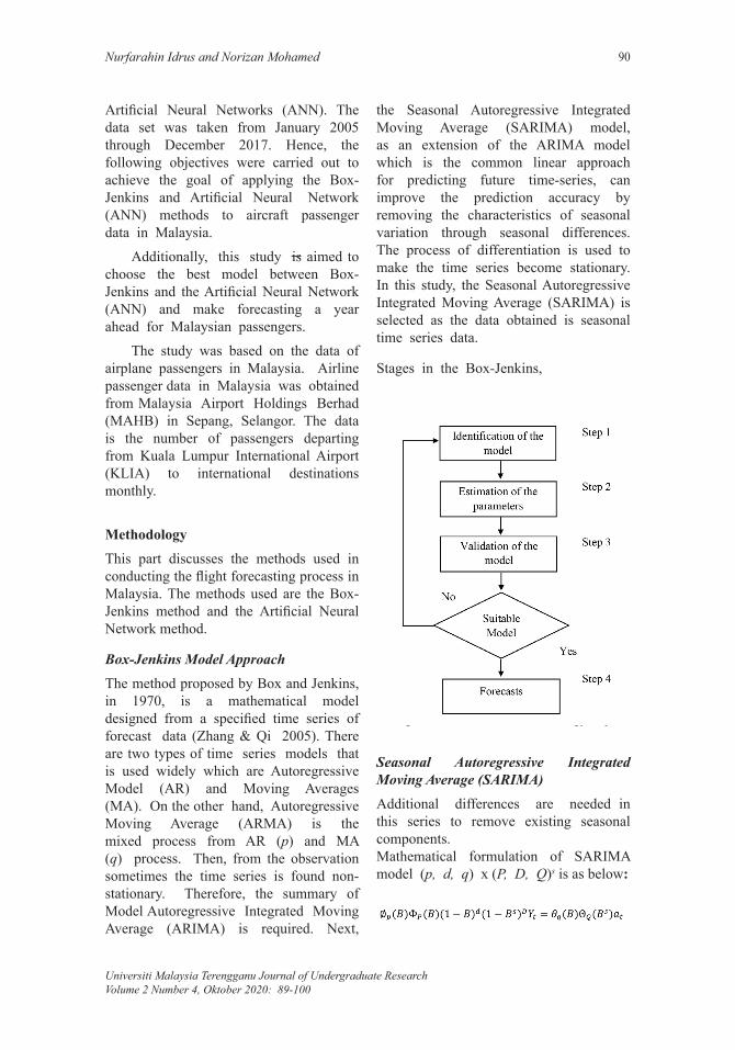
Box-Jenkins Model ApproachThe method proposed by Box and Jenkins, in 1970, is a mathematical model designed from a specified time series of forecast data (Zhang & Qi 2005). There are two types of time series models that is used widely which are Autoregressive Model (AR) and Moving Averages (MA). On the other hand, Autoregressive Moving Average (ARMA) is the mixed process from AR (p) and MA (q) process. Then, from the observation sometimes the time series is found non-stationary. Therefore, the summary of Model Autoregressive Integrated Moving Average (ARIMA) is required. Next,

the Seasonal Autoregressive Integrated Moving Average (SARIMA) model, as an extension of the ARIMA model which is the common linear approach for predicting future time-series, can improve the prediction accuracy by removing the characteristics of seasonal variation through seasonal differences. The process of differentiation is used to make the time series become stationary. In this study, the Seasonal Autoregressive Integrated Moving Average (SARIMA) is selected as the data obtained is seasonal time series data.

Stages in the Box-Jenkins,

Figure 1: Box-Jenkins methodology steps

Seasonal Autoregressive Integrated Moving Average (SARIMA)Additional differences are needed in this series to remove existing seasonal components. Mathematical formulation of SARIMA model (p, d, q) x (P, D, Q)s is as below:

with

FORECASTING THE NUMBER OF AIRPLANE PASSENGERS USING BOX-JENKINS AND ARTIFICIAL NEURAL NETWORK IN MALAYSIA 91


d : Differential sequence

s : Number of seasons D : Seasonal differential

Artificial Neural Network (ANN) Model ApproachThe Artificial Neural Network (ANN) approach is a model that is often found in the broad field of knowledge related to artificial intelligence (Khan 2018). It is based on mathematical models with the same architecture as the human brain. The neural network consists of a set of artificial neurons, nodes, perceptron or interconnected processing unit groups, which process and transmit information through activation functions. Feed-forward Neural Network is one of the simplest forms of ANN, where the data or the input travels in one direction. Besides, the back propagation is also a type of neural network. It is a group of connected I/O units where each connection has a weight associated with its computer programmes. Back propagation helps to build predictive models from large databases.

Multilayer Feed-Forward Neural Network (MFFNN)

The data enters input and passes the circuit, layer by layer, so it will reach the output. During a normal operation, which is when it works as a classifier, there is no feedback between layers. This is why they are called Multilayer Feed-Forward Neural Networks (MFFNN).

The most widely used ANN in prediction problems is MFFNN, which uses a scattering layer of feed layers. This model is characterized by a three-layer network, for example, inputs, hidden layers and outputs, which are linked by an acyclic link. There may be more than one hidden layer. Nodes in multiple layers are also known as processing elements. Three front layers

of ANN models can be illustrated as shown in Figure 2.

Figure 2: Multilayer feed-forward neural network (MFFNN)

The connection between the neurons are represented as weight. Each neuron consists of a function of summing and activation function. For the feed=forward network with N inputs nodes, H hidden nodes and one output node, the value Ŷ are given by :

with

wj : Output weight w0 : Bias g2 : Activation function

Therefore, the values of hidden nodes hj, j = 1,..., H are as follows :

with, vji : Input weight vj0 : Bias g1 : Activation functionyt-1 : Independent variables where

n=1,…,N



Evaluating Model PerformanceAfter predicting the airline passengers in Malaysia, tests were conducted to assess performance accuracy. Mean Absolute Percentage Error (MAPE), measures the accuracy of predicted prediction methods used in statistics . It states the accuracy as a percentage, and is defined by the formula:

with,

At : Original value of time tFt : Forecast value at time tn : Sample size

Table 1: Scale for MAPE from the Journal of Population Research (Swanson et. al., 2011)

MAPE Forecast AccuracyLess than 10% Very accurate

11% - 20% Accurate21% - 50% Reasonable forecast

More than 50% Not accurate

Results and DiscussionThis part discusses the prediction results of aircraft passengers in Malaysia using the Box-Jenkins method and the Artificial Neural Network.

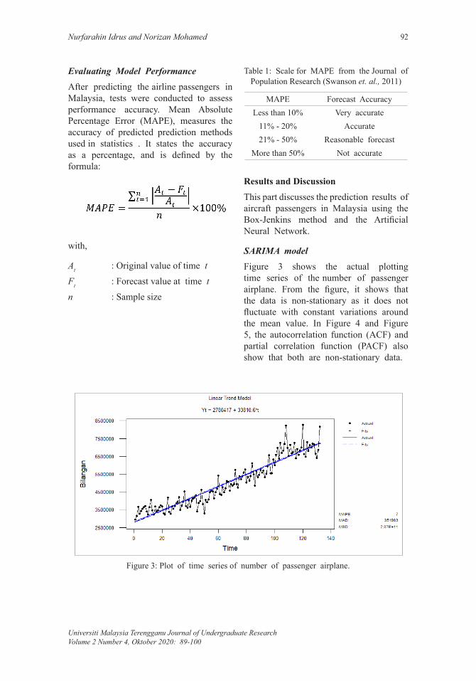
SARIMA modelFigure 3 shows the actual plotting time series of the number of passenger airplane. From the figure, it shows that the data is non-stationary as it does not fluctuate with constant variations around the mean value. In Figure 4 and Figure 5, the autocorrelation function (ACF) and partial correlation function (PACF) also show that both are non-stationary data.

Figure 3: Plot of time series of number of passenger airplane.



Figure 4: Autocorrelation function (ACF) of the number of passenger airplane.

Figure 5: Partial Autocorrelation function (PACF) of the number of passenger airplane.

is equal to 1. The value of p and q is observed by looking at the significant increase in Figure 7 and Figure 8. Moreover, from the figure, the estimated p and q values are 4 and 1 respectively since the PACF significant increase is 4 while the ACF significant increase is 1. Therefore, it can be said that, it is the non-seasonal part of the ARIMA model (4 , 1, 1).

Next, to solve the non-stationary data problem, differentiation method was applied to the original data to generate trends.

Figure 6 shows the time series fluctuating with the constant variation around the mean value after the first differentiation method and it was found that there are seasonal data components and the value of d in ARIMA (p, d, q)

Figure 6: Plot of time series after first differential method



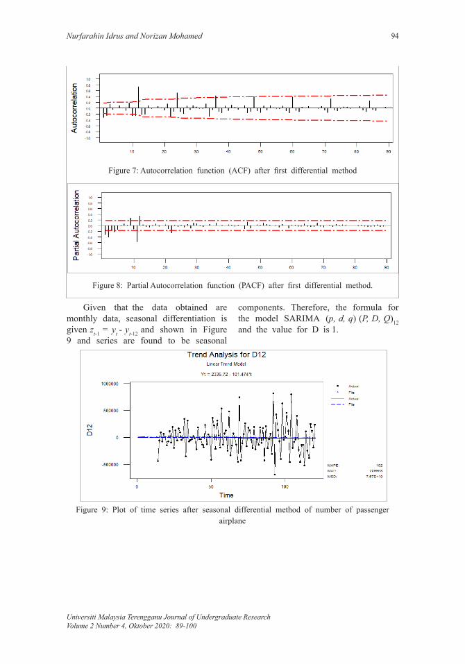
Figure 7: Autocorrelation function (ACF) after first differential method

Figure 8: Partial Autocorrelation function (PACF) after first differential method.

Given that the data obtained are monthly data, seasonal differentiation is given zt-1 = yt - yt-12 and shown in Figure 9 and series are found to be seasonal

components. Therefore, the formula for the model SARIMA (p, d, q) (P, D, Q)12 and the value for D is 1.

Figure 9: Plot of time series after seasonal differential method of number of passenger airplane



Figure 10: Autocorrelation function (ACF) after seasonal differential method of number of passenger airplane

Figure 11: Partial autocorrelation function (PACF) after seasonal differential method of number of passenger airplane

From Figures 10 and 11, it is found that time series on seasonal differentiation is stationary as ACF and PACF do not show trend presence and there is a significant increase in some lag. Therefore, the value of D is 1. Since there is no significant increase after the value of 12 on both diagrams, the values of P and Q are estimated to be 0. Subsequently, the seasonal part is SARIMA (0, 1, 0)12. and it can be said that the model to be studied is SARIMA (4, 1, 1)(0, 1, 0)12.

In addition, to build a model, a constant value δ should be assessed to determine whether it should be taken into account or vice versa. The calculation method is as follows:

Since the value of δ is less than 2, it does not count in terms of constant.

Model Estimation and Diagnostics Test

Final Estimates of ParametersType Coef StDev TAR 1 -0.5853 0.0949 -6.17AR 2 -0.2209 0.0951 -2.32

Differencing: 1 regular, 1 seasonal of order 12Number of observations: Original series 120, after differencing 107Residuals: SS = 6017317551581 (backforecasts excluded)MS = 57307786206 DF = 105

Figure 12: Estimated model parameters SARIMA

The stationary and variability of the parameters of the model are evaluated and summarised. Figure 12 shows the final estimation model parameter SARIMA (2, 1, 0)(0, 1, 0)12 after it was diagnosed from the SARIMA (4, 1, 1)(0, 1, 0)12, in which all type of ARs follow the standard |∅|<1 and θi< 1.



Best Box-Jenkins Model ApplicationSARIMA model is used to predict the number of passengers from January 2015 to December 2015. Table 2 shows the actual data and forecast data for the sample out data of the number of airplane passengers.

Table 2: Out-sample data value prediction

Months Initial Data Forecast Data

Jannuary 6636598 6927385February 6468735 6478524March 7303698 7137884April 6803763 6649544May 7132225 6713127Jun 6998083 7228778July 7208203 6365395

August 7165855 6874046September 6655645 6558399

October 6422676 6804425November 6868685 6976539December 8165603 8254842

To investigate the accuracy, MSE, RMSE and MAPE data in sample and out samples have been calculated. Table 3 shows the values obtained from the calculation.

Table 3: Results of MSE, RMSE, and MAPE.

Test SARIMA In sample MSE

RMSEMAPE

5.624237142.63.330253

Out sample MSERMSEMAPE

2.67011471709.12447.3458388

SARIMA model (2, 1, 0)(0, 1, 0)12 was selected as the best mode for prediction. The MSE, RMSE and MAPE values for the in sample data are 5.624 x 1010, 237142.6 and 3.330253 respectively. Whereas the value of MSE, RMSE and MAPE for the out sample data are 2.67011 x 1012, 471709.1244 and 7.3458388 respectively.

Figure 13: Plot forecast time series of number of passenger airplane

Figure 13 shows a plot of time series of forecasts of a number of passengers of a plane. The blue color trend shows the

upper limit and the lower limit while the red trend shows the forecasting value.



Artificial Neural Network (ANN) ModelThe lag variables of the previous SARIMA model , were used as input variables of the Artificial Neural Network model. We apply the log sigmoid function as transfer function in hidden layer and linear function

as transfer function in output layer. ). To find the best number of hidden nodes, all lag variables in the SARIMA (2,1,0)(0,1,0)12 model were used as input variables and the number of hidden nodes was increased from 1 to 10.

Table 4: Hidden layers for forward procedures

n MSETraining

MSETesting Training Testing MAPE

TrainingMAPETesting

1 0.1355 0.3454 0.9942 0.9946 10.4072 6.15832 0.085 0.2965 0.9964 0.9946 8.7216 5.19083 0.5528 0.0003 0.9977 0.9947 7.8532 5.66494 0.4347 0.0034 0.9982 0.9933 7.2276 6.21525 0.2765 0.0001 0.9988 0.994 6.669 0.00716 0.1596 0.0004 0.9993 0.9928 6.088 6.4147 0.061 0.0006 0.9997 0.9928 5.3178 8.3438 0.027 0.0005 0.9999 0.9942 4.8478 8.01419 0.0027 0.0001 9.9999 0.9902 4.322 0.007110 0.0088 0.0010 9.9999 0.9875 4.0558 10.5315

Multilayer Feed-Forward Neural Network (MFFNN)The best number of hidden node is 9. Then the f goal of 0.001 and hidden node

9 has been set with simulation tests 50 times to identify the best models by using different combination of input lag variables.

Table 5: Summary of Input Variable Results for Forward Procedures

Table 5 is a summary taken from Table 4. The best combination of input lag variables was selected based on a

comparison of MSE, R2 and MAPE. Once identified is the best combination of input lag variables



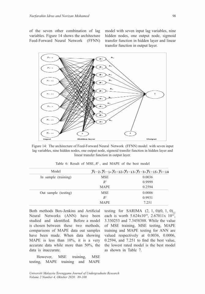
Figure 14: The architecture of Feed-Forward Neural Network (FFNN) model with seven input lag variables, nine hidden nodes, one output node, sigmoid transfer function in hidden layer and

linear transfer function in output layer.

Table 6: Result of MSE, R2 , and MAPE of the best model

ModelIn sample (training) MSE

R2

MAPE

0.00360.99990.2594

Out sample (testing) MSER2

MAPE

0.00060.99317.251

of the seven other combination of lag variables. Figure 14 shows the architecture Feed-Forward Neural Network (FFNN)

model with seven input lag variables, nine hidden nodes, one output node, sigmoid transfer function in hidden layer and linear transfer function in output layer.

Both methods Box-Jenkins and Artificial Neural Networks (ANN) have been studied and identified. Before a model is chosen between these two methods, comparisons of MAPE data out samples have been made. When data showing MAPE is less than 10%, it is a very accurate data while more than 50%, the data is inaccurate.

However, MSE training, MSE testing, MAPE training and MAPE

testing for SARIMA (2, 1, 0)(0, 1, 0)12 each is worth 5.624x1010, 2.67011x 1012, 3.330253 and 7.3458388. While the value of MSE training, MSE testing, MAPE training and MAPE testing for ANN are valued respectively at 0.0036, 0.0006, 0.2594, and 7.251 to find the best value, the lowest rated model is the best model as shown in Table 7.



Table 7: Comparison of Model Performance

Model Training TestingMSE MAPE MSE MAPE

SARIMA 5.624 3.330253 2.67011 7.34583880.0036 0.2594 0.0006 7.251

Acknowledgements In the name of Allah, the Most Gracious and the Most Merciful. Alhamdulillah, all praises to Allah for all His blessings and for giving me the strength in completing my thesis and I am so grateful that my thesis was selected for publication in the UMT Journal of Undergraduate Research. Special appreciation goes to my supervisor, Associate Professor Dr. Norizan Binti Mohamed, lecturer of School of Informatics and Applied Mathematics, for her supervision and support. She motivated me from the beginning until the completion of the project. Thank you for giving me the confidence to do the project successfully.

My deepest gratitude goes to my beloved parents: Mr. Idrus Bin Ashaari and Mrs. Norzila Binti Mohamat and also my siblings for all their endless love, prayers and support.

Last but not least, sincere thanks to all my friends especially Farahanim, Hafizin, Tengku, Ain, Athirah, ‘Aqilah, Ain Wahidah, Izzati, and others for their kindness and moral support during my study. Thank you for the friendship and memories. To those who indirectly contributed to this research, your kindness means a lot to me. Thank you very much.

ReferencesKhan, G. M. (2018). Artificial neural

network (ANNs). In Studies in Computational Intelligence. https://doi.org/10.1007/978-3-319-67466-7_4

ConclusionFor the Box-Jenkins method, after the data has undergone the first differential method, it was found that the data has seasonal components. Therefore, it is evident that the SARIMA model should be used for this study. Although it was originally the SARIMA model , which was identified as the model of investigation in the introduction of the model, model estimation and validation indicate that SARIMA is the best model for this study after being changed and studied. For Artificial Neural Networks (ANN), Feed-Forward Neural Network (FFNN) was one of the types of ANN selected. Various processes have been made to find inputs, hidden layers, and outputs using MATLAB. This process will produce an output which is the best model for the ANN method. After studying, is accepted as the best model.

Both models have been compared to identify the lowest MAPE data out samples. Studies show that the value of MAPE out sample for Box-Jenkins is 7.3458388 while for FFNN is 7.251. This decision clearly shows that the ANN is the best model compared to Box-Jenkins because it has fewer MAPE values.

The last objective was to predict the number of future airplane passenger from January 2015 to December 2015. As the component acquired is a seasonal one, this situation shows that forecasting is crucial to the number of passengers in Malaysia. This is because forecasting can help to plan more precisely and with helpful numbers.



Okulski, R. R., & Heshmati, A. (2010). Time Series Analysis of Global Airline Passengers Transportation Industry. Technology Management, Economics and Policy Program. Discussion Paper No. 2010:65 https://econpapers.repec.org/paper/snvdp2009/201065.htm

Swanson, D. A., Tayman, J., & Bryan, T. M. (2011). MAPE-R: A rescaled measure of accuracy for cross-sectional subnational population forecasts. Journal of Population Research, 28(2-3), 225-243. doi:10.1007/s12546-011-9054-5.

Zhang, G. P., & Qi, M. (2005). Neural network forecasting for seasonal and trend time series. European Journal of Operational Research. https://doi.org/10.1016/j.ejor.2003.08.037.

forecasting the number of airplane passengers using …

Documents