Forecasting Time Series Subject to Multiple Structural Breaks∗

M. Hashem PesaranUniversity of Cambridge and USC

Davide PettenuzzoBocconi University and Bates White LLC

Allan TimmermannUniversity of California, San Diego

November 2005

Abstract

This paper provides a new approach to forecasting time series that are subject to discretestructural breaks. We propose a Bayesian estimation and prediction procedure that allows forthe possibility of new breaks occuring over the forecast horizon, taking account of the size andduration of past breaks (if any) by means of a hierarchical hidden Markov chain model. Predic-

tions are formed by integrating over the parameters from the meta distribution that characterizesthe stochastic break point process. In an application to US Treasury bill rates, we find that themethod leads to better out-of-sample forecasts than a range of alternative methods.

Keywords: Structural Breaks, Forecasting, Hierarchical hidden Markov Chain, Bayesian Model Averag-

ing.

JEL Classifications: C110, C150, C530.

∗We thank two anonymous referees, the editor, Bernard Salanie, as well as Frank Diebold, Graham Elliott, John

Geweke, Jim Hamilton, Gary Koop, Ulrich Muller, Simon Potter, Mark Watson, Paolo Zaffaroni and seminar par-

ticipants at Cirano, Newton Institute of Mathematical Sciences at Cambridge University, the NBER 2005 Summer

meetings, UTS, Queen Mary College, London University and Monash University for comments on the paper.

1. Introduction

Structural changes or “breaks” appear to affect models for the evolution in key economic and

financial time series such as output growth, inflation, exchange rates, interest rates and stock

returns.1 This could reflect legislative, institutional or technological changes, shifts in economic

policy, or could even be due to large macroeconomic shocks such as the doubling or quadrupling of

oil prices experienced over the past decades.

A key question that arises in the context of time-series forecasting is how future values of the

variables of interest might be affected by breaks.2 If breaks have occurred in the past, surely they

are also likely to happen in the future. For forecasting purposes it is therefore not sufficient just to

identify past breaks, but it is also necessary that the stochastic process that underlies such breaks

is modeled. Questions such as how many breaks are likely to occur over the forecast horizon, how

large such breaks will be and at which dates they may occur need to be addressed. Approaches that

view breaks as being generated deterministically are not applicable when forecasting future events

unless, of course, future break dates as well as the size of such breaks are known in advance. In most

applications this is not a plausible assumption and modeling of the stochastic process underlying

the breaks is needed.

In this paper we provide a general framework for forecasting time series under structural breaks

that is capable of handling the different scenarios that arise once it is acknowledged that new

breaks can occur over the forecast horizon. Allowing for breaks complicates the forecasting problem

considerably. To illustrate this, consider the problem of forecasting some variable, y, h periods

ahead using a historical data sample {y1, ...., yT } in which the conditional distribution of y has beensubject to a certain number of breaks. First suppose that it is either known or assumed that no

new break occurs between the end of the sample, T , and the end of the forecast horizon, T + h. In

this case yT+h can be forecast based on the posterior parameter distribution from the last break

segment. Next, suppose that we allow for a single new break which could occur in any one of the

h different locations. Each break segment has a different probability assigned to it that must be

computed under the assumed breakpoint model. As the number of potential breaks grows, the

number of possible break locations grows more than proportionally, complicating the problem even

further.

Although breaks are found in most economic time-series, the likely paucity of breaks in a given

data sample means that a purely empirical approach to the identification of the break process would

not be possible, and a more structured approach is needed to learn about future breaks from past

1A small subset of the many papers that have reported evidence of breaks in economic and financial time series

includes Alogouskofis and Smith (1991), Ang and Bekaert (2002), Garcia and Perron (1996), Koop and Potter (2001,

2004a), Pastor and Stambaugh (2001), Pesaran and Timmermann (2002), Siliverstovs and van Dijk (2002), and Stock

and Watson (1996).2Clements and Hendry (1998, 1999) view structural breaks as the main source of forecast failure and introduce their

1999 book as follows: “Economies evolve and are subject to sudden shifts precipitated by legislative changes, economic

policy, major discoveries and political turmoil. Macroeconometric models are an imperfect tool for forecasting this

highly complicated and changing process. Ignoring these factors leads to a wide discrepancy between theory and

practice.”

1

breaks. For example, a formal modeling approach would be needed to exploit possible similarities of

the parameters across break segments. A narrow dispersion of the distribution of parameters across

breaks suggests that parameters from previous break segments contain considerable information on

the parameters after a subsequent break while a wider spread suggests less commonality and more

uncertainty about the nature of future breaks.

To model the break process we propose a hierarchical hidden Markov chain (HMC) approach

which assumes that the parameters within each break segment are drawn from some common meta

distribution. Our approach provides a flexible way of using all the sample information to compute

forecasts that embody information on the size and frequency of past breaks instead of discarding

observations prior to the most recent break point. As new regimes occur, the priors of the meta

distribution are updated using Bayes’ rule. Furthermore, uncertainty about the number of break

points during the in-sample period can be integrated out by means of Bayesian model averaging

techniques.

Our breakpoint detection, model selection and estimation procedures build on existing work in

the Bayesian literature including Gelman et al (2002), Inclan (1994), Kim, Nelson and Piger (2004),

Koop (2003), Koop and Potter (2004a,b), McCulloch and Tsay (1993) and, most notably, Chib

(1998). However, to handle forecasting outside the data sample we extend the existing literature

by allowing for the occurrence of random breaks drawn from the meta distribution. We apply the

proposed method in an empirical exercise that forecasts US Treasury Bill rates out-of-sample. The

results show the success of the Bayesian hierarchical HMC method that accounts for the possibility

of additional breaks over the forecast horizon vis-a-vis a range of alternative forecasting procedures

such as recursive and rolling least squares, a time-varying parameter model, and the random level

or variance shift models of McCulloch and Tsay (1993).

The paper is organized as follows: Section 2 generalizes the hidden Markov chain model of Chib

(1998) by extending it with a hierarchical structure to account for estimation of the parameters of

the meta distribution. Section 3 explains how to forecast future realizations under different break

point scenarios. Section 4 provides the empirical application, Section 5 conducts an out-of-sample

forecasting experiment, and Section 6 concludes. Appendices at the end of the paper provide

technical details.

2. Modeling the Break Process

Forecasting models used throughout economics make use of assumptions that relate variables in the

current information set to future realizations of the variable that is being predicted. For a given

forecasting model, this relationship can be represented through a set of distributions parameterized

by some vector, θ. Suppose, however, that the distribution of the predicted time-series given the

predictor variables is unstable over time and subject to discrete breaks. For example, in a given

historical sample, two breaks in the model parameters may have occurred at times τ1 and τ2,

giving rise to three sets of parameters, namely θ1 (the parameters before the first break), θ2 (the

parameters between the first and second break) and θ3 (the parameters after the second break).

2

The presence of parameter instability in the historical sample introduces a new source of risk from

the perspective of the forecaster and means that an understanding of how these parameters were

generated across different break segments becomes essential. When the parameters of a forecasting

model are subject to change, the predictive distribution, let alone the conditional mean, can only

be computed provided that parameter uncertainty following future breaks is integrated out. To

this end, we introduce in this paper a set of meta distributions which contain essential information

for forecasting. Intuitively, the meta distributions characterize the degree of similarity between the

parameters across different regimes. We propose an approach that not only accomplishes this, but

also updates posterior values of the parameters of the meta distribution optimally (using Bayes’

rule) given the evidence of historical (in-sample) breaks.

The idea that the parameters characterizing the data generating process within each break

segment are themselves drawn from some underlying distribution can be captured through the use

of a hierarchical prior. Intuition for the use of hierarchical priors comes from the shrinkage literature

since one can think of the parameters within the individual regimes as being shrunk towards a set

of so-called hyperparameters that characterize the ‘top’ layer of the hierarchy−in our case thedistribution from which the parameters of the individual regimes are drawn.

Using a hierarchical prior for the predictive densities has several advantages. First, hierarchical

priors can be viewed as mixtures of more primitive distributions and such mixtures are known to

provide flexible representations of unknown distributions. This is a particularly appealing aspect

when (as in many economic applications and ours in particular) economic theory has little to say

about how the distribution of the model parameters evolves through time. Second, while hierarchical

priors always have an equivalent non-hierarchical representation (see Koop (2003), p. 126), the

distribution of the hyperparameters provides potentially important information about the ‘risk’

associated with changes to model parameters across regimes. For example, if the variance of the

hyperparameters is large, there will be a greater chance of large shifts in the predictive density

following a break. Third, the use of hierarchical priors is often convenient numerically and hence

makes the approach more tractable and relatively easy to apply in practice.

More specifically, our break point model builds on the Hidden Markov Chain (HMC) formulation

of the multiple change point problem proposed by Chib (1998). Breaks are captured through an

integer-valued state variable, St = 1, 2, ...,K + 1 that tracks the regime from which a particular

observation, yt, of the target variable is drawn. Thus, st = l indicates that yt has been drawn from

f (yt| Yt−1,θl) , where Yt = {y1, ..., yt} is the current information set, θl =¡βl, σ

2l

¢represents the

location and scale parameters in regime l, i.e. θt = θl if τ l−1 < t ≤ τ l and ΥK = {τ0, ...., τK+1} isthe information set on the break points.3

The state variable St is modeled as a discrete state first order Markov process with the transition

probability matrix constrained to reflect a multiple change point model. At each point in time, Stcan either remain in the current state or jump to the next state. Conditional on the presence of K

3Throughout the paper we assume that τ0 = 0.

3

breaks in the in-sample period, the one-step-ahead transition probability matrix takes the form

P =

⎛⎜⎜⎜⎜⎜⎜⎜⎝

p11 p12 0 . . . 0

0 p22 p23 . . . 0...

......

......

0 . . . 0 pKK pK,K+1

0 0 . . . 0 1

⎞⎟⎟⎟⎟⎟⎟⎟⎠, (1)

where pj−1,j = Pr (st = j| st−1 = j − 1) is the probability of moving to regime j at time t given thatthe state at time t− 1 is j − 1. Note that pii + pi,i+1 = 1 and pK+1,K+1 = 1 due to the assumption

of K breaks which means that, conditional on K breaks occurring in the data sample, the process

terminates in state K + 1.4

Two issues are worth discussing in relation to the specification in (1). First, the assumption of

a constant transition probability (or, equivalently, a constant hazard rate) implies that the regime

duration follows a geometric distribution. Alternative specifications are possible−for example, Koopand Potter (2004b) propose a uniform prior on the break points or durations, while Koop and Potter

(2004a) propose a hierarchical prior setup that models the regime duration using a (conditional)

Poisson distribution. This approach leads to a non-homogenous transition probability matrix that

depends on the duration of each regime and puts prior weights on breaks that occur outside the

sample, but Koop and Potter develop estimation methods that can handle these potential compli-

cations.

Second, as argued by Koop and Potter (2004a,b), the assumption of a fixed number of regimes

may be too restrictive in many empirical applications. To address this issue and to avoid restricting

the in-sample or out-of-sample analysis by imposing a particular value of K, the number of in-

sample breaks, we show in Section 4 that uncertainty about K can be integrated out using Bayesian

model averaging techniques that combine forecasts from models that assume different numbers of

breaks.

The regime switching model proposed by Hamilton (1988) is a special case of this setup when

the parameters after a break are drawn from a discrete distribution with a finite number of states.

If identical states are known to recur, imposing this structure on the transition probability matrix

can lead to efficiency gains as it can lower the number of parameters that need to be estimated.

Conversely, wrongly imposing the assumption of recurring states will lead to inconsistent parameter

estimates.

To complete the specification of the break point process, we assume that the non-zero elements

of P, pii, are independent of pjj , j 6= i, and are drawn from a beta distribution,5

pii ∼ Beta (a, b) , for i = 1, 2...,K. (2)

4Strictly speaking the transition probability matrix, P, and the other model parameters, should be indexed by the

assumed number of breaks, K, and the sample size, T , i.e. PK,T . However, to keep the presentation as simple as

possible we do not use this notation.5Throughout the paper we use underscore bars (e.g. a) to denote parameters of a prior density.

4

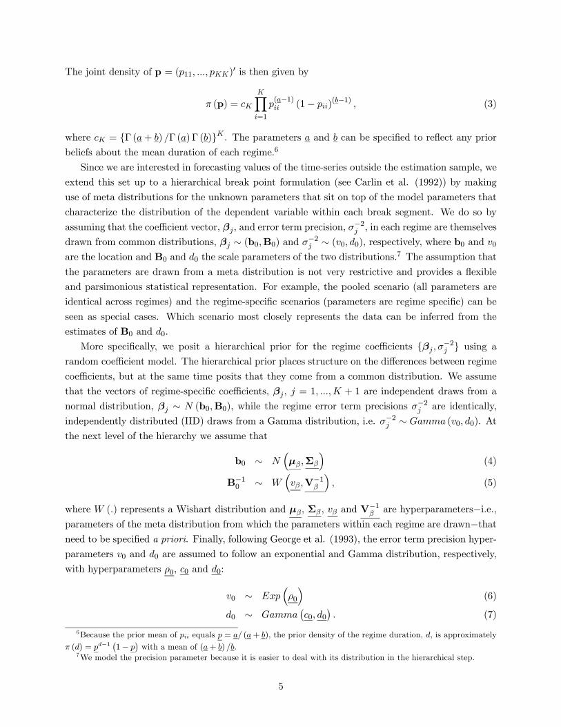
The joint density of p = (p11, ..., pKK)0 is then given by

π (p) = cK

KYi=1

p(a−1)ii (1− pii)

(b−1) , (3)

where cK = {Γ (a+ b) /Γ (a)Γ (b)}K . The parameters a and b can be specified to reflect any prior

beliefs about the mean duration of each regime.6

Since we are interested in forecasting values of the time-series outside the estimation sample, we

extend this set up to a hierarchical break point formulation (see Carlin et al. (1992)) by making

use of meta distributions for the unknown parameters that sit on top of the model parameters that

characterize the distribution of the dependent variable within each break segment. We do so by

assuming that the coefficient vector, βj , and error term precision, σ−2j , in each regime are themselves

drawn from common distributions, βj ∼ (b0,B0) and σ−2j ∼ (v0, d0), respectively, where b0 and v0

are the location and B0 and d0 the scale parameters of the two distributions.7 The assumption that

the parameters are drawn from a meta distribution is not very restrictive and provides a flexible

and parsimonious statistical representation. For example, the pooled scenario (all parameters are

identical across regimes) and the regime-specific scenarios (parameters are regime specific) can be

seen as special cases. Which scenario most closely represents the data can be inferred from the

estimates of B0 and d0.

More specifically, we posit a hierarchical prior for the regime coefficients {βj , σ−2j } using a

random coefficient model. The hierarchical prior places structure on the differences between regime

coefficients, but at the same time posits that they come from a common distribution. We assume

that the vectors of regime-specific coefficients, βj , j = 1, ...,K + 1 are independent draws from a

normal distribution, βj ∼ N (b0,B0), while the regime error term precisions σ−2j are identically,

independently distributed (IID) draws from a Gamma distribution, i.e. σ−2j ∼ Gamma (v0, d0). At

the next level of the hierarchy we assume that

b0 ∼ N³µβ,Σβ

´(4)

B−10 ∼ W³vβ,V

−1β

´, (5)

where W (.) represents a Wishart distribution and µβ, Σβ, vβ and V−1β are hyperparameters−i.e.,

parameters of the meta distribution from which the parameters within each regime are drawn−thatneed to be specified a priori. Finally, following George et al. (1993), the error term precision hyper-

parameters v0 and d0 are assumed to follow an exponential and Gamma distribution, respectively,

with hyperparameters ρ0, c0 and d0:

v0 ∼ Exp³ρ0

´(6)

d0 ∼ Gamma¡c0, d0

¢. (7)

6Because the prior mean of pii equals p = a/ (a+ b), the prior density of the regime duration, d, is approximately

π (d) = pd−1 1− p with a mean of (a+ b) /b.7We model the precision parameter because it is easier to deal with its distribution in the hierarchical step.

5

Appendix A contains details of how we estimate this model using the Gibbs sampler.8

This setup has a number of advantages and can be generalized in two main respects. First, it

is reasonably parsimonious and flexible as it draws the underlying regime parameters from simple

mixture distributions. However, one can readily adopt more flexible specifications for the distrib-

ution of the hyperparameters. This is most relevant in the analysis of time series that are subject

to a large number of breaks so the parameters of the meta distribution can be estimated with rea-

sonable precision. Second, the independence assumption across breaks can readily be relaxed either

by maintaining a time-series model for how the parameters {βj , σ−2j } evolve across regimes or by

relating them to a vector of observables. We provide more details of such extensions in Section 4.5

and 4.6.

2.1. Model Comparisons Under Different Numbers of Breaks

To assess how many break points (K) the data supports, we estimate separate models for a range

of sensible numbers of break points and then compare the results across these models. A variety

of classical and Bayesian approaches are available to select the appropriate number of breaks in

regression models. A classical approach that treats the parameters of the different regimes as given

and unrelated has been advanced by Bai and Perron (1998, 2003). This approach is not, however,

suitable for out-of-sample forecasting as it does not account for new regimes occurring after the end

of the estimation sample.

Here we adopt the Bayesian approach developed by Chib (1995, 1996) that is well suited

for model comparisons under high dimensional parameter spaces. Let the model with i breaks

be denoted by Mi. The method obtains an estimate of the marginal likelihood of each model,

f (y1, ..., yT |Mi), and ranks the different models by means of their Bayes factors:

Bij =f (y1, ..., yT |Mi)

f (y1, ..., yT |Mj),

where

f (y1, ..., yT |Mi) =f (y1, ..., yT |Mi,Θi,p)π (Θi,p|Mi)

π (Θi,p|Mi,YT ), (8)

Θi =¡β1, σ

21, ...,βi+1, σ

2i+1,b0,B0, v0, d0

¢.

Here YT = {y1, ..., yT}0 is the information set given by data up to the point of the prediction, T ,while Θi are the parameters of the model with i breaks (i ≥ 0).

The unknown parameters, Θi and p can be replaced by maximum likelihood estimates or by

their posterior means or modes. Large values of Bij indicate that the data supports Mi over Mj

(Jeffreys, 1961). Appendix B gives details of how the three components of (8) are computed.

8Maheu and Gordon (2004) also use a Bayesian method to forecasting under structural breaks but assume that the

post-break distribution is given by a subjective prior and do not apply a hierarchical hidden Markov chain approach

to update the prior distribution after a break.

6

2.2. Comparison with Other Approaches

It is insightful to compare our approach to that of McCulloch and Tsay (1993), who allow for

outlier detection in a time series in the form of shifts to either the level or variance of an rth order

autoregressive model. In the case of a level shift their model is given by

yt = β0,t + εt,

β0,t = β0,t−1 + δtγβ0t , (9)

εt =rX

i=1

βiεt−i + ut,

where Pr(δt = 1) = 1 − p, ut ∼ IIDN(0, σ2u) and γβ0t , the size of the level shift, is assumed to be

drawn from a known distribution. δt is a switching indicator so there is a break whenever δt = 1.

In case of a variance shift, the McCulloch and Tsay model takes the form

yt = β0 +rX

i=1

βiyt−i + ut,

ut ∼ N¡0, σ2t

¢(10)

σt = σt−1(1 + γσt δt),

where γσt is now the proportional shift in the standard deviation (1 + γσt > 0). According to these

models the probability of a break is 1 − p each period. Both models assume a partial break that

occurs either in the level or variance, but unlike in our setting does not affect the autoregressive

dynamics as captured by the coefficients (βi), or the duration of the regimes (p). Another difference

to our setup is that (9)-(10) are ‘random walk on random steps’ specifications and are therefore

fundamentally non-stationary models. They allow for the possibility of predicting breaks but,

unlike our approach, do not provide a method for characterizing and efficiently updating the (meta)

distribution from which the parameters across break segments and after a new break are drawn.

Our model also differs from standard time-varying parameter models βt = βt−1 + γt which

assume a (typically small) break in the location parameters every period. Instead, we allow for oc-

casional breaks that can affect both location and scale parameters and may introduce both random-

walk and/or mean-reverting behavior within different regimes. Furthermore, the probability of a

break varies across regimes as it depends on the realization of the stayer probability parameter, pii.

3. Posterior Predictive Distributions

In this section we show how to generate h−step-ahead out-of-sample forecasts from the model

proposed in Section 2. Having obtained the estimates of the break points and parameters in the

different regimes, we update the parameters of the meta distribution, b0,B0, v0, d0 and use this

information to forecast future values of y occurring after the end of our sample, T .

Conditional on the information set YT , density or point forecasts of the y process h steps

ahead, yT+h, can be made under a range of scenarios depending on what is assumed about the

7

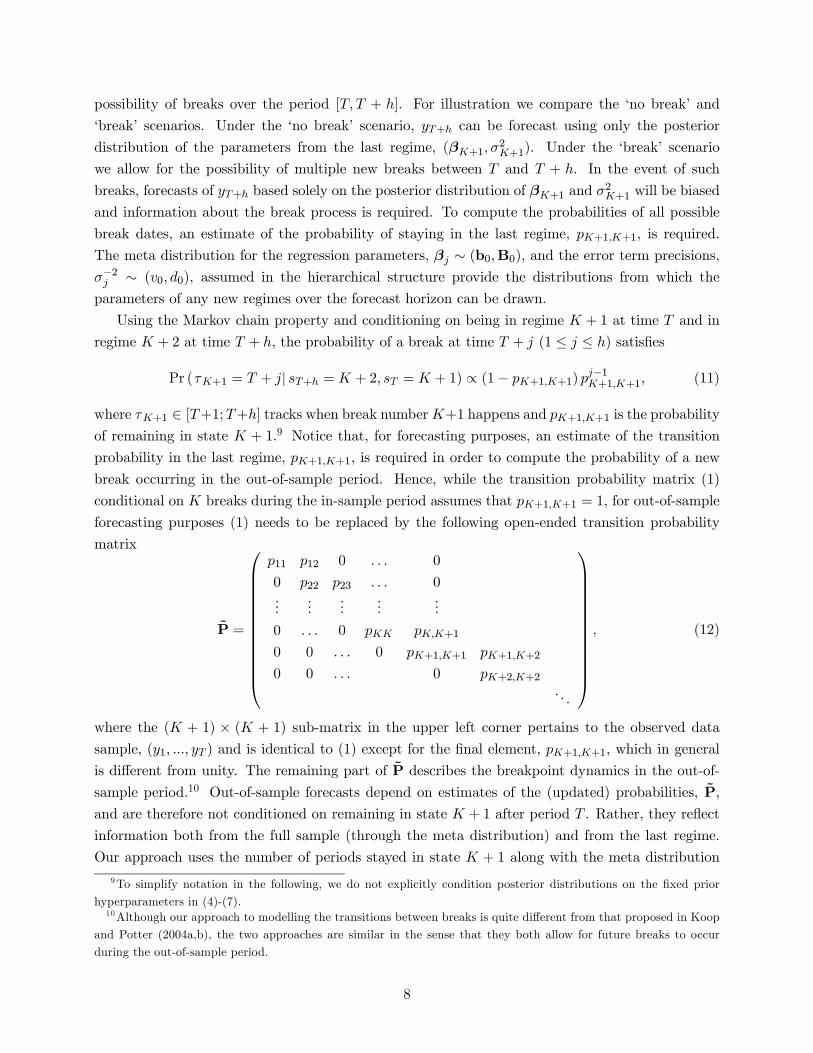
possibility of breaks over the period [T, T + h]. For illustration we compare the ‘no break’ and

‘break’ scenarios. Under the ‘no break’ scenario, yT+h can be forecast using only the posterior

distribution of the parameters from the last regime, (βK+1, σ2K+1). Under the ‘break’ scenario

we allow for the possibility of multiple new breaks between T and T + h. In the event of such

breaks, forecasts of yT+h based solely on the posterior distribution of βK+1 and σ2K+1 will be biased

and information about the break process is required. To compute the probabilities of all possible

break dates, an estimate of the probability of staying in the last regime, pK+1,K+1, is required.

The meta distribution for the regression parameters, βj ∼ (b0,B0), and the error term precisions,

σ−2j ∼ (v0, d0), assumed in the hierarchical structure provide the distributions from which the

parameters of any new regimes over the forecast horizon can be drawn.

Using the Markov chain property and conditioning on being in regime K + 1 at time T and in

regime K + 2 at time T + h, the probability of a break at time T + j (1 ≤ j ≤ h) satisfies

Pr (τK+1 = T + j| sT+h = K + 2, sT = K + 1) ∝ (1− pK+1,K+1) pj−1K+1,K+1, (11)

where τK+1 ∈ [T+1;T+h] tracks when break numberK+1 happens and pK+1,K+1 is the probabilityof remaining in state K + 1.9 Notice that, for forecasting purposes, an estimate of the transition

probability in the last regime, pK+1,K+1, is required in order to compute the probability of a new

break occurring in the out-of-sample period. Hence, while the transition probability matrix (1)

conditional on K breaks during the in-sample period assumes that pK+1,K+1 = 1, for out-of-sample

forecasting purposes (1) needs to be replaced by the following open-ended transition probability

matrix

P̃ =

⎛⎜⎜⎜⎜⎜⎜⎜⎜⎜⎜⎜⎜⎝

p11 p12 0 . . . 0

0 p22 p23 . . . 0...

......

......

0 . . . 0 pKK pK,K+1

0 0 . . . 0 pK+1,K+1 pK+1,K+2

0 0 . . . 0 pK+2,K+2. . .

⎞⎟⎟⎟⎟⎟⎟⎟⎟⎟⎟⎟⎟⎠, (12)

where the (K + 1) × (K + 1) sub-matrix in the upper left corner pertains to the observed data

sample, (y1, ..., yT ) and is identical to (1) except for the final element, pK+1,K+1, which in general

is different from unity. The remaining part of P̃ describes the breakpoint dynamics in the out-of-

sample period.10 Out-of-sample forecasts depend on estimates of the (updated) probabilities, P̃,

and are therefore not conditioned on remaining in state K + 1 after period T . Rather, they reflect

information both from the full sample (through the meta distribution) and from the last regime.

Our approach uses the number of periods stayed in state K + 1 along with the meta distribution

9To simplify notation in the following, we do not explicitly condition posterior distributions on the fixed prior

hyperparameters in (4)-(7).10Although our approach to modelling the transitions between breaks is quite different from that proposed in Koop

and Potter (2004a,b), the two approaches are similar in the sense that they both allow for future breaks to occur

during the out-of-sample period.

8

for the state transition parameters to obtain an updated estimate of pK+1,K+1, the probability of

remaining in state K + 1. Hence, information on the number of historical breaks (K) up to time

T is primarily used to estimate the time of the most recent break and to update the parameter

estimates of the meta distribution.

3.1. Uncertainty about Out-of-Sample Breaks

We next show how forecasts are computed under different out-of-sample scenarios before computing

a composite forecast as a probability-weighted average of the forecasts under each out-of-sample

breakpoint scenario and showing how to integrate out the uncertainty surrounding the number of

in-sample breaks.

3.1.1. No new Break

If it is assumed that there will be no break between T and T + h, the new data is generated from

the last regime (K + 1) in the observed sample. Then p (yT+h| sT+h = K + 1, yT ) is drawn fromR Rp¡yT+h|βK+1, σ

2K+1, sT+h = K + 1,YT

¢×π

¡βK+1, σ

2K+1|b0,B0, v0, d0,p,ST ,YT

¢dβK+1dσ

2K+1.

We thus proceed as follows:

Obtain a draw from π¡βK+1, σ

2K+1

¯̄b0,B0, v0, d0,p,ST ,YT

¢, where ST = (s1, ..., sT ) is the col-

lection of values of the latent state variable up to period T .

Draw yT+h from the posterior predictive density,

yT+h ∼ p¡yT+h|βK+1, σ

2K+1, sT+h = K + 1,YT

¢. (13)

3.1.2. Single out-of-sample Break

In this case, after a new break the process is generated under the parameters from (unobserved)

regime numberK+2. For a given break date, T+j (1 ≤ j ≤ h), p (yT+h| sT+h = K + 2, τK+1 = T + j,YT )is obtained fromZ

· · ·Z

p¡yT+h|βK+2, σ

2K+2,b0,B0, v0, d0, sT+h = K + 2, τK+1 = T + j,YT

¢×π

¡βK+2,b0,B0

¯̄YT¢× π

¡σ2K+2, v0, d0

¯̄YT¢dβK+2dσ

2K+2db0dB0dv0dd0.

To see how we update the posterior distributions of b0,B0, v0 and d0, define β1:K+1 =¡β01, ...,β

0K+1

¢0and σ21:K+1 =

¡σ21, ..., σ

2K+1

¢0. We then proceed as follows:Draw b0 from

b0 ∼ π¡b0|β1:K+1,σ21:K+1,B0, v0, d0,p,ST ,YT

¢,

9

and B0 from

B0 ∼ π¡B0|β1:K+1,σ21:K+1,b0, v0, d0,p,ST ,YT

¢.

Draw v0 from

v0 ∼ π¡v0|β1:K+1,σ21:K+1,b0,B0, d0,p,ST ,YT

¢,

and d0 from

d0 ∼ π¡d0|β1:K+1,σ21:K+1,b0,B0, v0,p,ST ,YT

¢.

Draw βK+2 and σ2K+2 from their priors given by π¡βK+2

¯̄b0,B0

¢and π

¡σ2K+2

¯̄v0, d0

¢, respec-

tively, for a fixed set of hyperparameters.

Draw yT+h from the posterior predictive density,

yT+h ∼ p¡yT+h|βK+2, σ

2K+2,b0,B0, v0, d0, sT+h = K + 2, τK+1 = T + j,YT

¢. (14)

To obtain the estimate of pK+1,K+1 needed in (11), we combine information from the last regime

with prior information, assuming the prior pK+1,K+1 ∼ Beta(a, b), so

pK+1,K+1| YT ∼ Beta(a+ nK+1,K+1, b+ 1), (15)

where nK+1,K+1 is the number of observations from regime K + 1.

3.1.3. Multiple out-of-sample Breaks

Assuming h ≥ 2, we can readily extend the previous discussion to multiple out-of-sample breaks.When considering the possibility of two or more breaks, we need an estimate of the probability of

staying in regime K + j, pK+j,K+j , j ≥ 2. This is not needed for the single break case since, byassumption, pK+2,K+2 is set equal to one. To this end we extend the hierarchical setup by adding

a prior distribution for the hyperparameters a and b of the transition probability,11

a ∼ Gamma¡a0, b0

¢, (16)

b ∼ Gamma¡a0, b0

¢.

values of pK+j,K+j are now drawn from the conditional beta posterior

pK+j,K+j |ΘK ,ΥK ,YT ∼ Beta(a+ li, b+ 1),

where li = τ i − τ i−1 − 1 is the duration of regime i and ΥK is the vector of in-sample break-point

parameters. The distribution for the hyperparameters a and b is not conjugate so sampling is

accomplished using a Metropolis-Hastings step. The conditional posterior distribution for a is

π (a|ΘK , τ ,p, b,YT ) ∝KQi=1

Beta (pii| a, b)Gamma¡a| a0, b0

¢.

11Following earlier notations, these parameters appear here without the underscore bar since they will be estimated

from the data.

10

To draw candidate values, we use a Gamma proposal distribution with shape parameter ς, mean

equal to the previous draw ag

q (a∗| ag) ∼ Gamma (ς, ς/ag) ,

and acceptance probability

ξ (a∗| ag) = min∙π (a∗|ΘK , τ ,P, b, y) /q (a

∗| ag)π (ag|ΘK , τ ,P, b, y) /q (ag| a∗)

, 1

¸.

Using these new posterior distributions, we generate draws for pK+2,K+2 based on the prior distri-

bution for the pii’s and the resulting posterior densities for a and b,12

pK+2,K+2| a, b ∼ Beta(a, b).

Allowing for up to nb breaks out-of-sample and integrating out uncertainty about their location,

we have

p(sT+h = K + 1|sT = K + 1,YT ) = phK+1,K+1

p(sT+h = K + 2|sT = K + 1,YT ) =hX

j1=1

(1− pK+1,K+1) pj1−1K+1,K+1

p(sT+h = K + 3|sT = K + 1,YT ) =h−1Xj1=1

hXj2=j1+1

pj1−1K+1,K+1 (1− pK+1,K+1) pj2−j1−1K+2,K+2 (1− pK+2,K+2)

...

p(sT+h = K + nb + 1|sT = K + 1,YT ) =h−nb+1Pj1=1

...hP

jnb=jnb−1+1

⎛⎝ nbYj=1

pdjK+j,K+j (1− pK+j,K+j)

⎞⎠ .

Using these equations, the predictive density that integrates out uncertainty both about the number

of out-of-sample breaks and about their location−but conditions on K in-sample breaks by setting

sT = K + 1, i.e., pK(yT+h|YT ) ≡ p (yT+h| sT = K + 1,YT )−can readily be computed:

pK (yT+h| YT ) =

nb+1Xj=1

pK (yT+h| sT+h = K + j, sT = K + 1,YT ) (17)

×p(sT+h = K + j|sT = K + 1,YT ).

3.2. Uncertainty about the Number of in-sample Breaks

So far we have shown how to integrate out uncertainty about the number of out-of-sample (future)

breaks. However, we have not dealt with the fact that we typically do not know the true number of

in-sample breaks in most empirical applications and so it is reasonable to integrate out uncertainty

about the right number of break points in the historical data.

12 In contrast to the case for pK+1,K+1, we do not have any information about the length of regime K +2 from the

estimation sample and rely on prior information to get an estimate of pK+2,K+2.

11

To integrate out uncertainty about the number of in-sample breaks, we compute the predictive

density as a weighted average of the predictive densities under the composite distributions, (17),

each of which conditions on a given number of historical breaks, K, using the model posteriors

as (relative) weights. We do this by means of Bayesian model averaging techniques. Let MK be

the model that assumes K breaks at time T (i.e., sT = K + 1). The predictive density under the

Bayesian model average is

p(yT+h|YT ) =K̄X

K=0

pK(yT+h|YT )p(MK |YT ), (18)

where K̄ is some upper limit on the largest number of breaks that is entertained. The weights used

in the average are given by the posterior model probabilities:

p (MK | YT ) ∝ f (y1, ..., yT |MK) p (MK) (19)

where f (y1, ..., yT |MK) is the marginal likelihood from (8) and p(MK) is the prior for model MK .

4. Empirical Application

We apply the proposed methodology to model U.S. Treasury Bill rates, a key economic variable

of general interest. This variable is ideally suited for our analysis since previous studies have

documented structural instability and regime changes in the underlying process, see Ang and Bekaert

(2002), Garcia and Perron (1996) and Gray (1996).

4.1. Data

We analyze monthly data on the nominal three month US T-bill rate from July 1947 through

December 2002. Prior to the beginning of this sample interest rates were fixed for a lengthy period

so our data set is the longest available post-war sample with variable interest rates. The data

source is the Center for Research in Security Prices at the Graduate School of Business, University

of Chicago. T-bill yields are computed from the average of bid and ask prices and are continuously

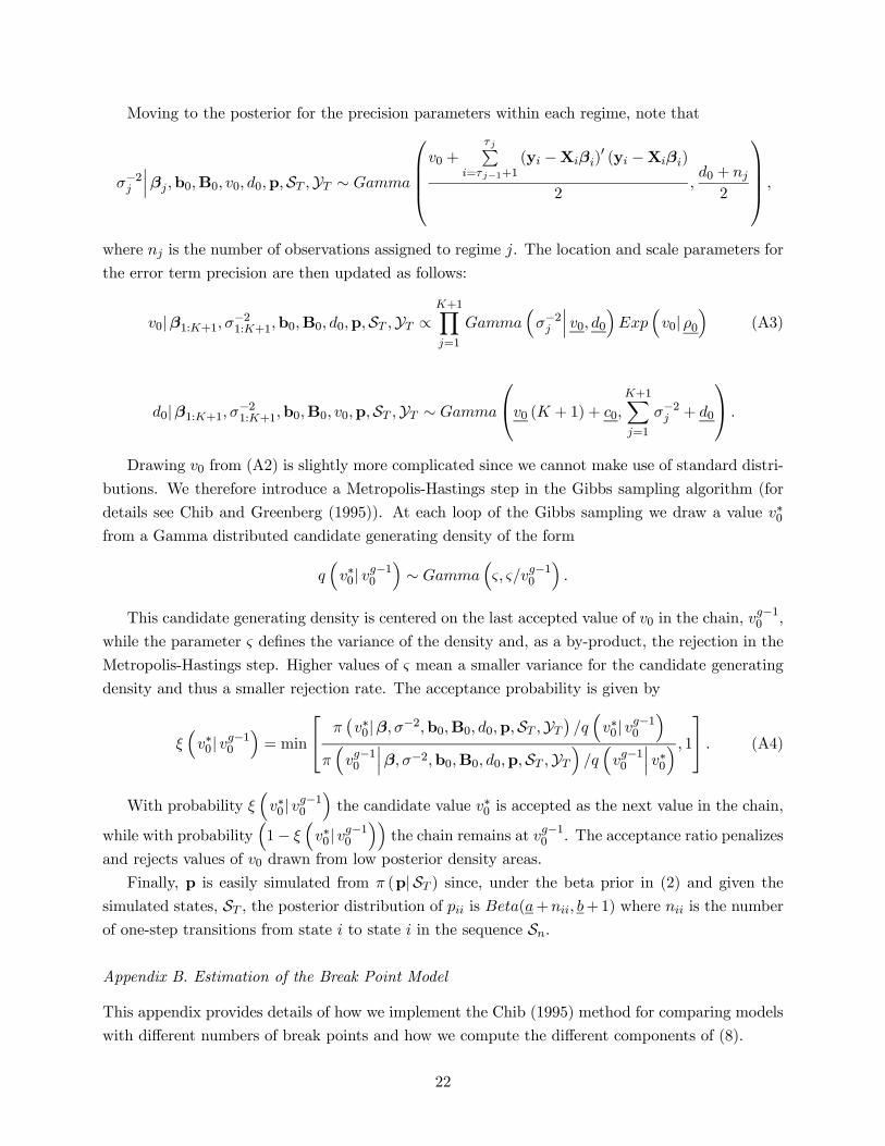
compounded 365 day rates. Figure 1 plots the monthly yields.

4.2. Prior Elicitation and Posterior Inference

In Section 2 we specified a Beta distribution for the diagonal elements of the transition probabil-

ity matrix, a Normal-Wishart distribution for the meta distribution parameters of the regression

coefficients and a Gamma-Exponential distribution for the error term precision parameters. Im-

plementation of our method requires assigning values to the associated hyperparameters. For the

pii-values we assume a non-informative prior for all the diagonal elements of (1), and set a = b = 0.5.

For the Normal-Wishart distribution, we specify µβ = 0, Σβ = 1000× Ir+1, vβ = 2 and Vβ = Ir+1,

where 0 is an (r + 1) × 1 vector of zeros, while Ir+1 is the (r + 1) × (r + 1) identity matrix andr + 1 is the number of elements of the location parameter, β. These values reflect no specific prior

12

knowledge and are diffuse over sensible ranges of values for both the Normal and Wishart distri-

bution. Similarly, we set ρ0 = 0.01, c0 = 1 and d0 = 0.01, allowing the prior for v0 and d0 to be

uninformative over the positive real line.

We also conducted a prior sensitivity analysis to ensure that the empirical results presented

below are robust to different prior beliefs. For the transition probability matrix, P, we modified a

and b to account for a wide set of regime durations; we also changed the beta prior hyperparameters

µβ and Σβ, and the regime error term precision hyperparameters c0, d0 and ρ0. In all cases we

found that the results were insensitive to changes in the prior hyperparameters.

More care, however, is needed when dealing with the prior precision hyperparameters, Vβ,

characterizing the dispersion of the location parameters across regimes. For small enough values

of its diagonal elements, the meta distribution for the regression coefficients will not allow enough

variation across regimes, and as a consequence the regime regression coefficients are clustered around

the mean of the meta distribution, b0. Empirical results were found to be robust for values of the

diagonal elements of Vβ greater than or equal to 1.

4.3. Model Estimates

In view of their empirical success and extensive use in forecasting,13 we model the process underlying

T-bill rates {yt} as an rth order autoregressive (AR) model allowing for up to K breaks over the

observed sample (y1, ....., yT ):

yt =

⎧⎪⎪⎪⎪⎨⎪⎪⎪⎪⎩β1,0 + β1,1yt−1 + ...+ β1,ryt−r + σ1 t, t = 1, ..., τ1

β2,0 + β2,1yt−1 + ...+ β2,ryt−r + σ2 t, t = τ1 + 1, ..., τ2...

βK+1,0 + βK+1,1yt−1 + ...+ βK+1,ryt−r + σK+1 t, t = τK + 1, ..., T.

(20)

Within the class of AR processes, this specification is quite general and allows for intercept and

slope shifts as well as changes in the error variances. Each regime j , j = 1, ...K+1, is characterized

by a vector of regression coefficients, βj =¡βj,0, βj,1, ...βj,r

¢0, and an error term variance, σ2j , for

t = τ j−1 + 1, ..., τ j .

Following previous studies of the T-bill rate, we maintain the AR(1) model as our base speci-

fication, but we also considered results for higher order AR models to verify the robustness of our

empirical findings. In each case we obtain a different model by varying the number of breaks, K,

and we rank these models by means of their marginal likelihoods computed using the method from

Section 2.1. Table 1 reports maximized log-likelihood values, marginal log-likelihoods and break

dates for values of K ranging from zero to seven. The maximized log-likelihood values are reported

for completeness and form an important ingredient in the model selection process. But since they

rise automatically as the number of breaks, and hence the number of parameters, is increased, on

their own they are not useful for model selection. To this end we turn to the marginal likelihoods

13See Pesaran and Timmermann (2005) for further references to the literature on forecasts from AR models subject

to breaks.

13

which penalize the likelihood values for overparameterization. Furthermore, under equal prior odds

for a pair of models, the posterior odds ratio commonly used for model selection will equal the ratio

of the models’ marginal likelihood values. For our data the marginal log-likelihood is maximized at

K = 6 and the model with K = 7 break points obtains basically the same marginal log-likelihood,

suggesting that the additional break is not supported by the data. Similar results were obtained

for an AR(2) specification.

Figure 2 plots the posterior probability for the six break points under the AR(1) model. The

local unimodality of the posterior distributions shows that the break points are generally precisely

estimated and appear sensible from an economic point of view: Breaks in 1979 and 1982 are as-

sociated with well-known changes to the Federal Reserve’s monetary policy, while the last break

occurs relatively shortly after the beginning of Alan Greenspan’s tenure as chairman of the Fed-

eral Reserve.14 For this model, Table 2 reports the autoregressive parameters, variance, transition

probability and the average number of months spent in each regime. In all regimes the interest

rate is highly persistent and close to a unit root process. The error term variance is particularly

high in regime 5 (lasting from October 1979 to October 1982, a period during which interest rate

fluctuations were very high), and quite low for regime 1 (September 1947 - November 1957), regime

3 (July 1960 - September 1966) and regime 7 (July 1989 - December 1997).

To get insight into the degree of commonality of model parameters across regimes, Table 3

reports prior parameter estimates, i.e. the meta distribution parameters. From the properties of

the Gamma distribution, the mean of the precision of the meta distribution is almost 18 and the

standard error is around 20. These values are consistent with the values of the inverse of the variance

estimates shown in Table 2.

4.4. Unit Root Dynamics

The persistent dynamics observed within some of the regimes may be a cause for concern when

calculating multi-step forecasts. Unit roots or even explosive roots could affect the meta distribution

that averages parameter values across the regimes. To deal with this problem, we propose the

following alternative constrained parameterization of the AR(1) model:

∆yt+1 = αjφj − φjyt + t+1, j = 1, ...,K + 1, (21)

where t+1 ∼ N(0, σ2j ). If φj = 0, the process has a unit root while if 0 < φj < 2, it is a stationary

AR(1) model. Notably, in the case with a unit root there is no drift irrespective of the value of αj .

Assuming that the process is stationary, its long run mean is simply αj .

We estimate our hierarchical HMC model under this new parameterization. To avoid explosive

roots and negative unconditional mean, we constrain φj to lie in [0, 1] and αj to be strictly positive.

We accomplish this by assuming that the priors for the regime regression parameters βj =¡αj , φj

¢014 In contrast, the plot for the model with seven break points (not shown here) had a very wide posterior density

for the 1976 break, providing further evidence against the inclusion of an additional break point.

14

and error term precisions are drawn from distributions

βj ∼ N (b0,B0) I¡βj ∈ A

¢, (22)

σ−2j ∼ Gamma (v0, d0) ,

while the priors for the meta-distribution hyperparameters in this case become

b0 ∼ N³µβ,Σβ

´I (b0 ∈ A) , (23)

B−10 ∼ W³vβ,V

−1β

´.

I (β ∈ A) in (22) and (23) is an indicator function that equals 1 if β belongs to the set A =

[0,∞)× (0, 1] and is zero otherwise. No changes are needed in the priors for the meta-distributionhyperparameters of the error term precision, v0 and d0. We obtain the same posterior densities as

under the unrestricted model although these distributions are now truncated due to the inequality

constraints.

Tables 4 and 5 report parameter estimates for this model, again assuming six breaks. The

detected break points are the same as those found for the unrestricted AR(1) model. To be com-

parable to the earlier tables, the regime coefficients and meta distribution results refer to αjφj and

1 − φj . The mean of the persistence parameter now varies from 0.88 (regime 2) to 0.991 (regime

1). Regimes 1 and 3 are more likely to be non-stationary as both have a unit root probability

slightly above one third. This is also reflected in the meta distribution results in Table 5 which

show that the probability of drawing a regime with a unit root is 0.38. Results for the remaining

hyperparameters are very close to those reported in Table 3.

4.5. Dependence in Parameters Across Regimes

So far we have assumed that the coefficient vector, βj , and error term precision, σ−2j , in each regime

are independent draws from common distributions. However, it is possible that these parameters

may be correlated across regimes and change more smoothly over time, so we consider a specification

that allows for autoregressive dynamics in the scale parameters across neighboring regimes, βj,i ∼(µi+ρiβj−1,i, σ

2η,i), i = 0, 1. We posit a hierarchical prior for the regime coefficients {βj , σ

−2j } so the

(r + 1)× 1 vectors of regime-specific coefficients, βj , j = 1, ...,K + 1 are correlated across regimes,

i.e. βj ∼¡µ+ ρβj−1,Ση

¢, where ρ is a diagonal matrix, while we continue to assume that the

error term precisions σ−2j are IID draws from a Gamma distribution, i.e. σ−2j ∼ Gamma (v0, d0).

As for the earlier specification in (4) and (5), at the level of the meta distribution we assume that

(µ,ρ) ∼ N³µβ,Σβ

´(24)

Σ−1η ∼ W³vβ,V

−1β

´, (25)

where µβ, Σβ, vβ and V−1β are again hyperparameters that need to be specified a priori. We

continue to assume that the error term precision hyperparameters v0 and d0 follow an exponential

and Gamma distribution, see (6)-(7).

15

Results under this specification are shown in Table 6 and should be compared with those reported

in Table 4. The changes in the intercept and autoregressive parameter estimates within each regime

are minor and fall well within the standard error bands for these parameters. Furthermore, the

estimates in Table 7 show that there is only little persistence in the intercept and autoregressive

parameters across regimes; in both cases the mean of the parameter characterizing persistence across

regimes (ρi) is below one-half and less than two standard errors away from zero.

4.6. Heteroskedasticity, non-Gaussian Innovations and Variance Breaks

Another potential limitation to the results is that the assumption of Gaussian innovations may

not be accurate and the innovations could have fatter tails. To account for this possibility, one

can let the innovations in (20), t, follow a student-t distribution, i.e. t ∼ IID t³0, σ2j , vλ

´for

τ j−1 ≤ t ≤ τ j , with vλ the degrees of freedom parameter. When this model was fitted to our data,

empirical estimates that continue to allow for intercept and slope shifts as well as changes in the

error variances across regimes were very similar to those reported in Table 4. The main change was

that the autoregressive parameter in the second regime (from 1947 to 1957) was somewhat lower

and the innovation variance a bit higher in some of the regimes.

Allowing the residuals to be drawn from a student-t distribution is one way to account for

unconditional heteroskedasticity. Another issue that may be relevant when forecasting T-Bill rates

is the possible presence of autoregressive conditional heteroskedasticity (ARCH) in the residuals.

In our framework ARCH effects can be explicitly accounted for through a Griddy Gibbs sampling

approach, c.f. Bauwens and Lubrano (1998), although this will be computationally cumbersome.

To a large extent our approach deals with heteroskedasticity by letting the innovation variance

vary across regimes so the volatility parameter effectively follows a step function. To investigate

if the normalized residuals (scaled by the estimated standard deviation) from our model remain

heteroskedastic, we ran Lagrange Multiplier tests, regressing the squared normalized residuals on

their lagged values. Even though some ARCH effects remain, after scaling the residuals by the

posterior estimates of the standard deviation, we found that the R2 of the Lagrange Multiplier

regression was reduced from 12% to 2%.

Testing for breaks that exclusively affect the variance provides further insights into the interest

rate series. When we estimated a model with breaks that only affect the variance parameters similar

to the variance shift specification proposed by McCulloch and Tsay (1993), we continued to find

evidence of multiple breaks. Some of these are similar to the breaks identified by our more general

specification−such as the breaks in 1979 and 1982, suggesting that variance shifts are an integralpart of the breakpoint process.15

15When fitted to our data, the McCulloch and Tsay (1993) level shift model identified two breaks, the last occurring

in 1980, while the variance shift model identified 12 break points. The reason why the latter model identifies more

breaks than our composite model is that we allow for simultaneous breaks in the mean and variance parameters. In

contrast, the variance shift model is a partial break model and may therefore require more breaks in the variance to

fit the data than a model that allows the conditional mean dynamics to change through time as well.

16

4.7. Uncertainty about the Number of in-sample Breaks

The empirical results presented thus far were computed from the hierarchical HMC model under the

assumption of six breaks during the in-sample period. As mentioned in Section 3.2, however, one can

argue that it is not reasonable to condition on a particular number of historical breaks. We therefore

explicitly consider models with different numbers of break points, integrating out uncertainty about

the number of break points in the data by means of the Bayesian model averaging formulas (18)-

(19). Specifically, we consider between zero and seven breaks and assign equal prior probabilities to

each of these scenarios. Our results reveal that a probability mass close to zero is assigned to the

models with five or fewer break points while 76 and 24 percent of the posterior mass is assigned to

the models with six and seven break points, respectively.

To gauge the importance of uncertainty about the number of historical breaks, the solid line

in Figure 3 plots the combined predictive density under Bayesian model averaging along with the

predictive density that conditions on six breaks, both computed as of 1997:12, the last point for

which a five-year forecast can be evaluated. The graphs reveal that the two densities are very

similar. At least in this particular application, it appears to make little difference whether one

conditions on six in-sample breaks or integrates out uncertainty about the number of breaks.

5. Forecasting Performance

To assess the forecasting performance of our method, we undertook a recursive out-of-sample fore-

casting exercise that compares our model with seven alternative approaches in common use. These

include a model that assumes no new breaks so that the parameters from the last regime remain in

effect in the out-of-sample period (see Section 3.1.1), a time-varying parameter model that lets the β

parameters follow a random walk, the random level shift and random variance shift autoregressive

models of McCulloch and Tsay (1993) given in equations (9) and (10), a recursive least squares

model that uses an expanding estimation window and finally two rolling window least squares mod-

els with window lengths set at five and ten years, respectively. Such rolling windows provide a

popular way of dealing with parameter instability. The hierarchical forecasting model considers

all possible out-of-sample break point scenarios in (17). We refer to this as the composite-meta

forecast.16 To obtain the predictive density under the no new break scenario we use information

from the last regime of the hierarchical model as in (14). All forecasts are based on an AR(1)

specification, but predictive distributions under an AR(2) model are very similar.

We next explain details of how the time-varying parameter and random shift models were es-

timated. For the time-varying parameter model we adopted Zellner’s g-prior (Zellner (1986)) and

considered the specification

yt = x0t−1βt + t, t ∼ N¡0, σ2

¢βt = βt−1 + υt, υt ∼ N

£0, δ2σ2(X0X)−1

¤.

16This forecast sets the priors at a0 = 1 and b0 = 0.1. Different values for a0 and b0 were tried and the results were

found to be robust to changes in a0, b0.

17

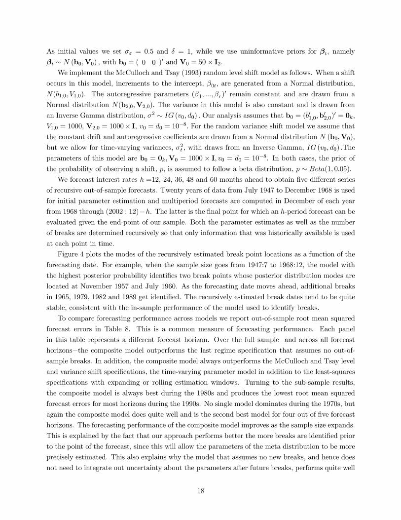
As initial values we set σε = 0.5 and δ = 1, while we use uninformative priors for βt, namely

βt ∼ N (b0,V0) , with b0 = ( 0 0 )0 and V0 = 50× I2.We implement the McCulloch and Tsay (1993) random level shift model as follows. When a shift

occurs in this model, increments to the intercept, β0t, are generated from a Normal distribution,

N(b1,0, V1,0). The autoregressive parameters (β1, ..., βr)0 remain constant and are drawn from a

Normal distribution N(b2,0,V2,0). The variance in this model is also constant and is drawn from

an Inverse Gamma distribution, σ2 ∼ IG (v0, d0) . Our analysis assumes that b0 = (b01,0,b02,0)

0 = 0k,

V1,0 = 1000, V2,0 = 1000× I, v0 = d0 = 10−8. For the random variance shift model we assume that

the constant drift and autoregressive coefficients are drawn from a Normal distribution N (b0,V0),

but we allow for time-varying variances, σ2t , with draws from an Inverse Gamma, IG (v0, d0) .The

parameters of this model are b0 = 0k,V0 = 1000 × I, v0 = d0 = 10−8. In both cases, the prior of

the probability of observing a shift, p, is assumed to follow a beta distribution, p ∼ Beta(1, 0.05).

We forecast interest rates h =12, 24, 36, 48 and 60 months ahead to obtain five different series

of recursive out-of-sample forecasts. Twenty years of data from July 1947 to December 1968 is used

for initial parameter estimation and multiperiod forecasts are computed in December of each year

from 1968 through (2002 : 12)−h. The latter is the final point for which an h-period forecast can beevaluated given the end-point of our sample. Both the parameter estimates as well as the number

of breaks are determined recursively so that only information that was historically available is used

at each point in time.

Figure 4 plots the modes of the recursively estimated break point locations as a function of the

forecasting date. For example, when the sample size goes from 1947:7 to 1968:12, the model with

the highest posterior probability identifies two break points whose posterior distribution modes are

located at November 1957 and July 1960. As the forecasting date moves ahead, additional breaks

in 1965, 1979, 1982 and 1989 get identified. The recursively estimated break dates tend to be quite

stable, consistent with the in-sample performance of the model used to identify breaks.

To compare forecasting performance across models we report out-of-sample root mean squared

forecast errors in Table 8. This is a common measure of forecasting performance. Each panel

in this table represents a different forecast horizon. Over the full sample−and across all forecasthorizons−the composite model outperforms the last regime specification that assumes no out-of-sample breaks. In addition, the composite model always outperforms the McCulloch and Tsay level

and variance shift specifications, the time-varying parameter model in addition to the least-squares

specifications with expanding or rolling estimation windows. Turning to the sub-sample results,

the composite model is always best during the 1980s and produces the lowest root mean squared

forecast errors for most horizons during the 1990s. No single model dominates during the 1970s, but

again the composite model does quite well and is the second best model for four out of five forecast

horizons. The forecasting performance of the composite model improves as the sample size expands.

This is explained by the fact that our approach performs better the more breaks are identified prior

to the point of the forecast, since this will allow the parameters of the meta distribution to be more

precisely estimated. This also explains why the model that assumes no new breaks, and hence does

not need to integrate out uncertainty about the parameters after future breaks, performs quite well

18

at the beginning of the out-of-sample experiment, i.e. during the 1970s when relatively few breaks

had been identified.

Since the predictive densities are highly non-normal, root mean squared forecast error compar-

isons provide at best a partial view of the various models’ forecasting performance. A more complete

evaluation of the predictive densities that can be applied to the Bayesian forecasting models (namely

the last regime model and the McCulloch and Tsay (1993) random level and variance shift models),

is provided by the predictive Bayes factor. This measure can be applied for pair-wise model compar-

ison, c.f. Geweke and Whiteman (2005). A value greater than one suggests out-performance of the

benchmark model which in our case is the composite model. Since the posterior distributions for

the different scenarios do not have simple closed form solutions, we compute the predictive Bayes

factors as follows. To get the predictive Bayes factor that compares, say, the last regime (lr) model

against the composite (c) model for a particular time period t, we first generate, for both models,

an empirical probability density function (pdf) by using a kernel estimator.17 The predictive Bayes

factor for c against lr is given by the ratio of their pdfs evaluated at the realized value yt,

BF lrt =

fc¡yt|βlr, σ

2lr,Yt−1

¢flr (yt|βc, σ

2c ,Yt−1)

.

A number greater than one suggests that the composite model better predicts yt than the last regime

model. This calculation is performed for each observation in the recursive forecasting exercise and

the average value across the sample is reported.

Empirical results are shown in Table 9. Across all subsamples, the composite model produces

Bayes factors that exceed unity and thus performs better than the last regime model (no new break)

and random level and variance shift specifications.

6. Conclusion

The key contribution of this paper was to introduce a hierarchical hidden Markov chain approach to

model the meta distribution of the parameters of the stochastic process underlying structural breaks.

This allowed us to forecast economic time series that are subject to unknown future breaks. When

applied to autoregressive specifications for U.S. T-Bill rates, an out-of-sample forecasting exercise

found that our approach produces better forecasts than a range of alternative methods that either

ignore the possibility of future breaks, assume a break every period (as in the time-varying parameter

model) or allow for shifts in the mean or variance during the in-sample period (as in McCulloch

and Tsay (1993)). Our approach is quite general and can be implemented in different ways from

that assumed in the current paper. For example, the state transitions could be allowed to depend

on time-varying regressors tracking factors related to uncertainty about institutional shifts or the

likelihood of macroeconomic or oil price shocks.

The simple ‘no new break’ approach that forecasts using parameter estimates solely from the last

post-break period can be expected to perform well when the number of observations from the last

17Results did not appear to be sensitive to the choice of kernel estimator, but the results reported here are obtained

using an Epanechinov kernel with Silverman bandwidth, see Silverman (1986).

19

regime is sufficiently large to deliver precise parameter estimates, and the possibility of new breaks

occurring over the forecast horizon is very small, see Pesaran and Timmermann (2005). However,

when forecasting many periods ahead or when breaks occur relatively frequently, so the last break

point is close to the end of the sample and a new break is likely to occur shortly after the end of

the estimation sample, this approach is unlikely to produce satisfactory forecasts.

Intuition for why our approach appears to work quite well in forecasting interest rates is that it

effectively shrinks the new parameters drawn after a break towards the mean of the meta distribu-

tion. Shrinkage has widely been found to be a useful device for improving forecasting performance

in the presence of parameter estimation and model uncertainty, see, e.g., Diebold and Pauly (1990),

Stock and Watson (2004), Garratt, Lee, Pesaran and Shin (2003), and Aiolfi and Timmermann

(2004). Here it appears to work because the number of breaks that can be identified empirically

tends to be small and the parameters of the meta distribution from which such breaks are drawn

are reasonably precisely estimated.

Appendix A. Gibbs Sampler for the Multiple Break Point Model

The posterior distribution of interest is π (Θ,p,ST | YT ), where, under the assumption of K in-

sample breaks18

Θ =¡β1, σ

21, ...,βK+1, σ

2K+1,b0,B0, v0, d0

¢includes the K + 1 regime coefficients and the prior locations and scales, ST = (s1, ..., sT ) is the

collection of values of the latent state variable, YT = (y1, ..., yT )0, and p = (p11, p22,..., pKK)0 sum-

marizes the unknown parameters of the transition probability matrix in (1). The Gibbs sampler

applied to our set up works as follows. First the states ST are simulated conditional on the data,YT , and the parameters, Θ, and, second, the parameters, Θ, are simulated conditional on the data,YT , and ST . Specifically, the Gibbs sampling is implemented by simulating the following set ofconditional distributions:

1. π (ST |Θ,p,YT )

2. π (Θ, | YT ,p,ST )

3. π (p| ST ) ,

where we have used the identity π (Θ,p| ST ,YT ) = π (Θ| YT ,p,ST )π (p| ST ), noting that underour assumptions π (p|Θ,ST ,YT ) = π (p| ST ).

The simulation of the states ST requires ‘forward’ and ‘backward’ passes through the data.

Define St = (s1, ..., st) and St+1 = (st+1, ..., sT ) as the state history up to time t and from time t to

T , respectively. We partition the states’ joint density as follows:

p(sT−1| YT , sT ,Θ,p)× · · · × p(st| YT ,St+1,Θ,p)× · · · × p(s1| YT ,S2,Θ,p). (A1)

18For simplicity, throughout this appendix we drop the subscript, K, and refer to ΘK as Θ.

20

Chib (1995) shows that the generic element of (A1) can be decomposed as

p(st| YT ,St+1,Θ,p) ∝ p(st| YT ,Θ,p)p(st| st−1,Θ,p), (A2)

where the normalizing constant is easily obtained since st takes only two values conditional on

the value taken by st+1. The second term in (A2) is simply the transition probability from the

Markov chain. The first term can be computed by a recursive calculation (the forward pass through

the data) where, for given p(st−1| Yt−1,Θ,p), we obtain p(st| Yt,Θ,p) and p(st+1| Yt+1,Θ,p), ...,p(sT | Yt,Θ,p). Suppose p(st−1| Yt−1,Θ,p) is available, then

p(st = k| Yt,Θ,p) =p(st = k| Yt−1,Θ,p)× f (yt| Yt−1,Θk)kX

l=k−1p(st = l| Yt−1,Θ,p)× f (yt| Yt−1,Θl)

,

where, for k = 1, 2, ...,K + 1,

p(st = k| Yt−1,Θ,p) =kX

l=k−1plk × p(st−1 = l| Yt−1,Θ,p),

and plk is the Markov transition probability.

For a given set of simulated states, ST , the data is partitioned into K+1 groups. To obtain theconditional distributions for the regression parameters, prior locations and scales, note that in the

model in Section 2 the conditional distributions of the βj ’s are mutually independent with

βj

¯̄σ2j ,b0,B0, v0, d0,p,ST ,YT ∼ N

¡βj , V j

¢,

where

Vj =¡σ−2X0jXj +B

−10

¢−1, βj = Vj

¡σ−2X0jyj +B

−10 b0

¢,

Xj is the matrix of observations on the regressors in regime j, and yj is the vector of observations

on the dependent variable in regime j.

Defining β1:K+1 =¡β01, ...,β

0K+1

¢0 and σ21:K+1 = ¡σ21, ..., σ

2K+1

¢0, the densities of the locationand scale parameters of the regression parameter meta-distribution, b0 and B0, can be written

b0|β1:K+1,σ21:K+1,B0, v0, d0,p,ST ,YT ∼ N¡µβ,Σβ

¢B−10

¯̄β1:K+1,σ

21:K+1,b0, v0, d0,p,ST ,YT ∼ W

³vβ,V

−1β

´,

where

Σβ =³Σ−1β + (K + 1)B−10

´−1µβ = Σβ

ÃB−10

JPj=1

βj +Σ−1β µβ

!,

and

vβ = vβ + (K + 1)

Vβ =JPj=1

¡βj − b0

¢ ¡βj − b0

¢0+Vβ.

21

Moving to the posterior for the precision parameters within each regime, note that

σ−2j

¯̄̄βj ,b0,B0, v0, d0,p,ST ,YT ∼ Gamma

⎛⎜⎜⎜⎝v0 +

τjPi=τj−1+1

(yi −Xiβi)0 (yi −Xiβi)

2,d0 + nj2

⎞⎟⎟⎟⎠ ,

where nj is the number of observations assigned to regime j. The location and scale parameters for

the error term precision are then updated as follows:

v0|β1:K+1, σ−21:K+1,b0,B0, d0,p,ST ,YT ∝K+1Yj=1

Gamma³σ−2j

¯̄̄v0, d0

´Exp

³v0| ρ0

´(A3)

d0|β1:K+1, σ−21:K+1,b0,B0, v0,p,ST ,YT ∼ Gamma

⎛⎝v0 (K + 1) + c0,K+1Xj=1

σ−2j + d0

⎞⎠ .

Drawing v0 from (A2) is slightly more complicated since we cannot make use of standard distri-

butions. We therefore introduce a Metropolis-Hastings step in the Gibbs sampling algorithm (for

details see Chib and Greenberg (1995)). At each loop of the Gibbs sampling we draw a value v∗0from a Gamma distributed candidate generating density of the form

q³v∗0| v

g−10

´∼ Gamma

³ς, ς/vg−10

´.

This candidate generating density is centered on the last accepted value of v0 in the chain, vg−10 ,

while the parameter ς defines the variance of the density and, as a by-product, the rejection in the

Metropolis-Hastings step. Higher values of ς mean a smaller variance for the candidate generating

density and thus a smaller rejection rate. The acceptance probability is given by

ξ³v∗0| v

g−10

´= min

⎡⎣ π¡v∗0|β, σ−2,b0,B0, d0,p,ST ,YT

¢/q³v∗0| v

g−10

´π³vg−10

¯̄̄β, σ−2,b0,B0, d0,p,ST ,YT

´/q³vg−10

¯̄̄v∗0

´ , 1⎤⎦ . (A4)

With probability ξ³v∗0| v

g−10

´the candidate value v∗0 is accepted as the next value in the chain,

while with probability³1− ξ

³v∗0| v

g−10

´´the chain remains at vg−10 . The acceptance ratio penalizes

and rejects values of v0 drawn from low posterior density areas.

Finally, p is easily simulated from π (p| ST ) since, under the beta prior in (2) and given thesimulated states, ST , the posterior distribution of pii is Beta(a+nii, b+1) where nii is the number

of one-step transitions from state i to state i in the sequence Sn.

Appendix B. Estimation of the Break Point Model

This appendix provides details of how we implement the Chib (1995) method for comparing models

with different numbers of break points and how we compute the different components of (8).

22

Consider the points (Θ∗,p∗) in (Θ,p), which could be maximum likelihood estimates or poste-

rior means or modes. The likelihood function evaluated at Θ∗ and p∗ is available from the proposed

parameterization of the change point model and can be obtained as

log f ((y1, ..., yT )|Θ∗,p∗) =TXt=1

log f (yt| Yt−1,Θ∗,p∗) ,

where the one-step-ahead predictive density is

f (yt| Yt−1,Θ∗,p∗) =K+1Xk=1

f (yt| Yt−1,Θ∗,p∗, st = k) p (st = k| Yt−1,Θ∗,p∗) .

For simplicity we suppressed the model indicator. The prior density evaluated at the posterior

means or modes is easily computed since it is known in advance. The denominator of (8) needs

some explanation, however. We can decompose the posterior density as

π (Θ∗, P ∗| YT ) = π (Θ∗| YT )π (p∗|Θ∗,YT ) ,

where

π (Θ∗| YT ) =Z

π (Θ∗| YT ,ST ) p (ST | YT ) dST ,

and

π (p∗|Θ∗,YT ) =Z

π (p∗| ST )π (ST |Θ∗,YT ) dST .

The first part can be estimated as bπ (Θ∗| YT ) = G−1GPg=1

π (Θ∗| YT ,ST,g) using G draws from the

run of the Markov Chain Monte Carlo algorithm, [ST,g]Gg=1. The second part π (p∗|Θ∗,YT ) requiresan additional simulation of the Gibbs sampler from π (ST |Θ∗,YT ). These draws are obtained byadding steps at the end of the original Gibbs sampling in order to simulate ST conditional on

(YT ,Θ∗,p∗) and p∗ conditional on (YT ,Θ∗,ST ).The idea outlined above is easily extended to the case where the Gibbs sampler divides Θ into

B blocks, i.e. Θ =¡Θ(1),Θ(2), ...,Θ(B)

¢. Since

π (Θ∗| YT ) = π³Θ∗(1)

¯̄̄YT´π³Θ∗(2)

¯̄̄Θ∗(1),YT

´· · ·π

³Θ∗(B)

¯̄̄Θ∗(1), ...,Θ

∗(B−1),YT

´,

we can use different Gibbs sampling steps to calculate the posterior π (Θ∗| Y). In our example wehave Θ(1) = βj , Θ(2) = σ−2j (j = 1, ...,K + 1), Θ(3) = b0, Θ(4) = B0, Θ(5) = v0 and Θ(6) = d0.

The Chib method can become computationally demanding, but the various sampling steps all have

the same structure. For some of the blocks in the hierarchical Hidden Markov Chain model, the full

conditional densities are non-standard, and sampling requires the use of the Metropolis-Hastings

algorithm (see for example the precision prior hyperparameter v0). The Chib (1995) algorithm is

then modified following Chib and Jeliazkov (2001).

23

References

Aiolfi, M. and A. Timmermann, 2004, Persistence in Forecasting Performance and Conditional Combination

Strategies. Forthcoming in Journal of Econometrics.

Alogoskoufis, G.S. and R. Smith, 1991, The Phillips Curve, the Persistence of Inflation, and the Lucas

Critique: Evidence from Exchange Rate Regimes. American Economic Review 81, 1254-1275.

Ang, A., and G., Bekaert, 2002, Regime Switches in Interest Rates, Journal of Business and Economic

Statistics, 20, 163-182.

Bai, J. and P. Perron, 1998, Estimating and Testing Linear Models with Multiple Structural Changes.

Econometrica 66, 47-78.

Bai, J. and P. Perron, 2003, Computation and Analysis of Multiple Structural Change Models, Journal of

Applied Econometrics, 18, 1-22.

Bauwens, L. and M. Lubrano, 1998, Bayesian Inference on GARCH Models using the Gibbs Sampler. Econo-

metrics Journal, 1, C23-C46.

Carlin, B., A.E. Gelfand and A.F.M. Smith, 1992, Hierarchical Bayesian analysis of changepoint problems,

Applied Statistics, 41, 389-405.

Chib, S., 1995, Marginal Likelihood from the Gibbs output, Journal of the American Statistical Association,

90, 1313-1321.

Chib, S., 1996, Calculating Posterior Distribution and Modal Estimates in Markov Mixture Models, Journal

of Econometrics, 75, 79-97.

Chib, S., 1998, Estimation and Comparison of Multiple Change Point Models, Journal of Econometrics, 86,

221-241.

Chib, S. and E. Greenberg, 1995, Understanding the Metropolis-Hastings Algorithm, American Statistician,

49, 327-335.

Chib, S. and I. Jeliazkov, 2001, Marginal Likelihood from the Metropolis-Hastings Output, Journal of the

American Statistical Association, 96, 270-281.

Clements, M.P. and D.F. Hendry, 1998, Forecasting Economic Time Series, Cambridge University Press.

Clements, M.P. and D.F. Hendry, 1999, Forecasting Non-stationary Economic Time Series, The MIT Press.

Diebold, F.X and P. Pauly, 1990, The Use of Prior Information in Forecast Combination, International

Journal of Forecasting, 6, 503-508.

Garratt, A, K. Lee, M. H. Pesaran and Y. Shin, 2003, Forecast Uncertainties in Macroeconometric Modelling:

An Application to the UK Economy. Journal of the American Statistical Association, 98, 829-838.

24

Garcia, R. and P. Perron, 1996, An Analysis of the Real Interest Rate under Regime Shifts. Review of

Economics and Statistics, 78, 111-125.

Gelman, A., J.B. Carlin, H.S. Stern and D. Rubin, 2002, Bayesian Data Analysis, Second Edition, Chapman

& Hall Editors.

George, E. I., U. E. Makov and A. F. M. Smith, 1993, Conjugate Likelihood Distributions, Scandinavian

Journal of Statistics, 20, 147-156.

Geweke, J. and C. H. Whiteman, 2005, Bayesian Forecasting. Forthcoming in Elliott, G., C.W.J. Granger

and A. Timmermann (eds.), Handbook of Economic Forecasting. North Holland.

Gray, S., 1996, “Modeling the Conditional Distribution of Interest Rates as Regime-Switching Process”,

Journal of Financial Economics, 42, 27-62.

Hamilton, J.D., 1988, Rational Expectations Econometric Analysis of Changes in Regime. An Investigation

of the Term Structure of Interest Rates. Journal of Economic Dynamics and Control, 12, 385-423.

Inclan, C., 1994, Detection of Multiple Changes of Variance Using Posterior Odds. Journal of Business and

Economic Statistics, 11, 289-300.

Jeffreys, H., 1961, Theory of Probability, Oxford University Press, Oxford.

Kim, C.J., C.R. Nelson and J. Piger, 2004, The Less-Volatile US Economy. A Bayesian Investigation of

Timing, Breadth, and Potential Explanations. Journal of Business and Economic Statistics 22, 80-93.

Koop, G., 2003, Bayesian Econometrics, John Wiley & Sons, New York.

Koop, G. and S. Potter, 2001, Are Apparent Findings of Nonlinearity Due to Structural Instability in Eco-

nomic Time Series? Econometrics Journal, 4, 37-55.

Koop, G. and S. Potter, 2004a, Forecasting and Estimating Multiple Change-point Models with an Unknown

Number of Change-points. Mimeo, University of Leicester and Federal Reserve Bank of New York.

Koop, G. and S. Potter, 2004b, Prior Elicitation in Multiple Change-point Models. Mimeo, University of

Leicester and Federal Reserve Bank of New York.

Maheu, J.M. and S. Gordon, 2004, Learning, Forecasting and Structural Breaks. Manuscript University of

Toronto.

McCulloch, R.E. and R. Tsay, 1993, Bayesian Inference and Prediction for Mean and Variance Shifts in

Autoregressive Time Series. Journal of the American Statistical Association 88, 965-978.

Pastor, L. and R.F. Stambaugh, 2001, The Equity Premium and Structural Breaks. Journal of Finance, 56,

1207-1239.

Pesaran, M.H. and A. Timmermann, 2002, Market Timing and Return Prediction under Model Instability.

Journal of Empirical Finance, 9, 495-510.

25

Pesaran, M.H. and A. Timmermann, 2005, Small Sample Properties of Forecasts from Autoregressive Models

under Structural Breaks. Journal of Econometrics, 129, pp. 183-217.

Siliverstovs, B. and D. van Dijk, 2002, Forecasting Industrial Production with Linear, Non-linear and Struc-

tural Breaks Models. Manuscript DIW Berlin.

Silverman, B.W., 1986, Density Estimation for Statistics and Data Analysis. London: Chapman and Hall.

Stock, J.H. and M.W. Watson, 1996, Evidence on Structural Instability in Macroeconomic Time Series

Relations, Journal of Business and Economic Statistics, 14, 11-30.

Stock, J.H. and M.W. Watson, 2004, Combination Forecasts of Output Growth in a Seven-Country Data

Set. Journal of Forecasting, 23, 405-430..

Zellner, A., 1986, On Assessing Prior Distributions and Bayesian Regression Analysis with g-Prior Distribu-

tions. In Goel, P.K. and Zellner, A. (eds.) , Bayesian Inference and Decision Techniques: Essays in Honour

of Bruno de Finetti. Amsterdam: North-Holland.

26

Figure 1: Monthly T-Bill rates, 1947:7 - 2002:12.

27

Figure 2: Posterior probability of break occurrence, assuming K = 6 breaks.

28

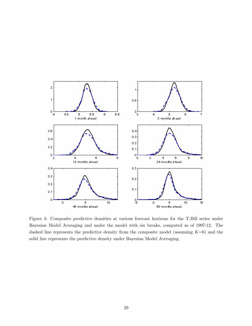
Figure 3: Composite predictive densities at various forecast horizons for the T-Bill series under

Bayesian Model Averaging and under the model with six breaks, computed as of 1997:12. The

dashed line represents the predictive density from the composite model (assuming K=6) and the

solid line represents the predictive density under Bayesian Model Averaging.

29

Figure 4: Break point locations for the recursive out-of-sample forecasting exercise. The horizontal

axis shows the forecasting date and the stars represent the associated posterior distribution modes

for the probability of break occurrence.

30

No. of breaks Log lik.(LL) Marginal LL Break dates

0 -477.131 -508.434

1 -372.563 -466.707 Oct-69

2 -255.398 -372.674 Oct-69 May-85

3 -223.208 -353.792 Oct-69 Sep-79 Sep-82

4 -205.617 -346.497 Oct-57 Sep-79 Sep-82 Jun-89

5 -174.699 -338.321 May-53 Oct-69 Sep-79 Sep-82

Jun-89

6 -140.154 -315.611 Oct-57 Jun-60 Aug-66 Sep-79

Sep-82 Jun-89

7 -130.086 -316.713 Oct-57 Jun-60 Aug-66 Jan-76

Sep-79 Sep-82 Jun-89

Table 1: Model comparison. This table shows the log likelihood and the marginal log likelihood

estimates for different numbers of breaks along with the time of the break points for the first-order

autoregressive model.

Parameter estimates

Regimes

1 2 3 4 5 6 7

date 47-57 57-60 60-66 66-79 79-82 82-89 89-02

Constant

Mean 0.021 0.252 0.017 0.220 0.412 0.246 -0.004

s.e. 0.034 0.208 0.067 0.161 0.521 0.211 0.054

AR(1) coefficient

Mean 1.002 0.895 1.006 0.969 0.958 0.968 0.992

s.e. 0.020 0.071 0.020 0.026 0.045 0.027 0.011

Variances

Mean 0.023 0.256 0.015 0.260 2.558 0.161 0.048

s.e. 0.003 0.068 0.003 0.031 0.671 0.027 0.005

Transition Probability matrix

Mean 0.988 0.960 0.979 0.991 0.961 0.981 1

s.e. 0.010 0.032 0.017 0.008 0.032 0.015 0

Mean dur. 120 37 72 156 37 84 99

Table 2: Posterior parameter estimates for the unconstrained AR(1) hierarchical Hidden Markov

Chain model with six break points.

31

Mean Parameters

Mean s.e. 95% conf interval

b0(1) 0.166 0.221 -0.174 0.699

b0(2) 0.972 0.173 0.528 1.253

Variance Parameters

Mean s.e.

B0(1, 1) 0.296 0.249

B0(2, 2) 0.202 0.148

Error term precision

Mean s.e. 95% conf interval

v0 0.825 0.326 0.360 1.405

d0 0.046 0.024 0.014 0.094

Table 3: Prior parameter estimates for the unconstrained AR(1) hierarchical Hidden Markov Chain

model with six break points.

Parameter estimates

Regimes

1 2 3 4 5 6 7

date 47-57 57-60 60-66 66-79 79-82 82-89 89-02

αjφjMean 0.029 0.303 0.055 0.244 0.546 0.279 0.044

s.e. 0.029 0.184 0.054 0.140 0.431 0.175 0.033

1− φjMean 0.991 0.877 0.990 0.965 0.947 0.964 0.983

s.e. 0.011 0.064 0.012 0.022 0.037 0.023 0.007

Pr¡φj = 0

¢0.379 0.016 0.369 0.0319 0.044 0.019 0

Variances

Mean 0.023 0.257 0.016 0.258 2.504 0.159 0.048

s.e. 0.003 0.072 0.003 0.030 0.613 0.025 0.005

Transition Probability matrix

Mean 0.988 0.960 0.980 0.991 0.960 0.982 1

s.e. 0.010 0.031 0.016 0.008 0.031 0.014 0

Mean dur. 120 37 72 156 37 84 99

Table 4: Posterior parameter estimates for the AR(1) hierarchical Hidden Markov Chain model

with six break points under the constrained parameterization in (22).

32

Mean Parameters

Mean s.e. 95% conf interval

b0(1) 0.165 0.192 0 0.705

b0(2) 0.916 0.106 0.540 1

Pr (b0(2) = 1) 0.379

Variance Parameters

Mean s.e.

B0(1, 1) 0.273 0.249

B0(2, 2) 0.179 0.124

Error term precision

Mean s.e. 95% conf interval

v0 0.884 0.397 0.377 1.681

d0 0.050 0.029 0.015 0.106

Table 5: Prior parameter estimates for the AR(1) hierarchical Hidden Markov Chain model with

six break points under the constrained parameterization in (22).

Parameter estimates

Regimes

1 2 3 4 5 6 7

date 47-57 57-60 60-66 66-79 79-82 82-89 89-02

αjφjMean 0.031 0.290 0.070 0.265 0.763 0.368 0.045

s.e. 0.030 0.178 0.062 0.143 0.622 0.209 0.034

1− φjMean 0.990 0.890 0.985 0.961 0.931 0.951 0.982

s.e. 0.012 0.062 0.016 0.023 0.052 0.028 0.007

Pr¡φj = 0

¢0.351 0.022 0.245 0.032 0.041 0.012 0

Variances

Mean 0.023 0.243 0.024 0.257 2.443 0.174 0.049

s.e. 0.003 0.067 0.009 0.030 0.583 0.034 0.006

Transition Probability matrix

Mean 0.988 0.960 0.980 0.991 0.960 0.982 1

s.e. 0.010 0.031 0.016 0.008 0.031 0.014 0

Table 6: Posterior parameter estimates for the AR(1) hierarchical Hidden Markov Chain model

with six break points under beta dependency across regimes (equations (25)-(26)).

33

Mean Parameters

Mean s.e. 95% conf interval

µ1 0.174 0.296 -0.277 0.632

ρ1 0.414 0.270 0.032 0.900

µ2 0.489 0.324 -0.022 0.994

ρ2 0.485 0.292 0.042 0.947

Variance Parameters

Mean s.e.

Ση,1,1 0.441 0.806

Ση,2,2 0.160 0.203

Error term precision

Mean s.e. 95% conf interval

v0 0.955 0.407 0.418 1.793

d0 0.062 0.035 0.018 0.131

Table 7: Prior parameter estimates for the AR(1) hierarchical Hidden Markov Chain model with

six break points under beta dependency across regimes (equations (25)-(26)).

34

h=12

Com- Last Random Random TVP Rec Rolling Rolling

posite regime Level Variance OLS Win 5 Win 10

68-2002 1.900 2.033 3.246 2.093 2.504 1.938 2.334 2.071

70s 2.336 2.297 2.414 2.130 2.059 2.301 2.649 2.530

80s 1.679 2.132 5.129 2.503 3.157 1.905 2.367 1.918

90s 1.630 1.688 1.545 1.673 2.270 1.597 2.001 1.723

h=24

68-2002 2.698 2.974 5.878 3.570 5.841 3.089 4.244 3.276

70s 3.205 3.172 4.358 3.796 3.289 3.765 4.471 3.916

80s 2.766 3.451 9.406 4.339 8.082 3.281 5.444 3.324

90s 2.167 2.356 2.245 2.604 5.296 2.245 2.746 2.637

h=36

68-2002 3.005 3.324 7.941 4.572 9.646 3.571 6.268 3.772

70s 3.366 3.231 5.221 4.472 4.341 4.148 6.268 4.625

80s 3.531 4.217 12.941 6.112 13.189 4.285 8.714 3.911

90s 2.191 2.510 2.744 2.979 9.067 2.313 3.334 2.906

h=48

68-2002 3.060 3.454 10.078 5.232 13.986 3.662 8.755 4.107

70s 3.072 2.653 4.176 3.924 5.137 3.525 8.952 5.104

80s 3.902 4.694 17.017 7.684 18.426 5.004 12.419 4.148

90s 2.192 2.676 2.954 3.223 13.750 2.254 3.850 3.310

h=60

68-2002 3.194 3.677 12.115 6.268 18.826 3.875 13.529 4.966

70s 3.169 2.663 3.476 3.519 5.113 3.482 15.205 7.331

80s 4.157 4.943 20.519 9.640 22.883 5.530 18.984 4.358

90s 2.201 2.929 2.886 3.536 20.026 2.145 4.550 3.655

Table 8: Root mean squared forecast errors at different forecast horizons h for the full sample

(1968-2002) and for different sub-samples. Root mean squared forecast errors are computed using

the posterior means of the predictive densities under the constrained composite Hierarchical Hid-

den Markov Chain model, the model assuming no new breaks after the end of the sample (Last

regime), the Random Level-Shift (Random Level) and the Random Variance-Shift (Random Vari-

ance) Autoregressive models of McCulloch and Tsay (1993), the Time Varying Parameter (TVP),

the Recursive OLS (Rec OLS) and the Rolling Window OLS methods, with window length of five

(Rolling Win 5) or ten years (Rolling Win 10).

35

h=12

Full smpl 70s 80s 90s

Last regime 1.113 1.139 1.135 1.067

RL-AR 3.546 7.415 2.420 1.053

RV-AR 1.399 1.655 1.210 1.321

h=24

Full smpl 70s 80s 90s

Last regime 1.184 1.349 1.114 1.104

RL-AR 1.555 2.163 1.494 1.129

RV-AR 1.571 2.548 1.249 1.025

h=36

Full smpl 70s 80s 90s

Last regime 1.312 1.237 1.072 1.547

RL-AR 1.568 2.256 1.292 1.283

RV-AR 1.558 2.635 1.3237 0.992

h=48

Full smpl 70s 80s 90s

Last regime 1.148 1.195 1.004 1.229

RL-AR 1.522 1.809 1.541 1.331

RV-AR 1.623 2.743 1.481 1.042

h=60

Full smpl 70s 80s 90s

Last regime 1.115 1.029 0.933 1.300

RL-AR 1.610 1.735 1.813 1.401

RV-AR 1.841 3.015 1.884 1.177

Table 9: Predictive Bayes factor at different forecast horizons h and different sub-samples. The

predictive densities under the composite Hierarchical Hidden Markov Chain model (Composite) is

taken as the benchmark and is compared with the model assuming no new breaks after the end

of the sample (Last regime), the Random Level-Shift (RL-AR) and the Random Variance-Shift

(RV-AR) Autoregressive models of McCulloch and Tsay (1993).

36