Forecasting UK inflation bottom up

Andreas Joseph

Bank of England?

Joint work with Eleni Kalamara (KCL & ECB), George Kapetanios (KCL)

and Galina Potjagailo (BoE)

Nontraditional Data & Statistical Learning with Applications to Macroeconomics

BoI & FRB, virtual, 11. November 2020

?Disclaimer: The expressed views are my own and not necessarily those of the Bank of England (BoE) or European Central Bank (ECB). All errors

are ours.

Introduction

Motivation

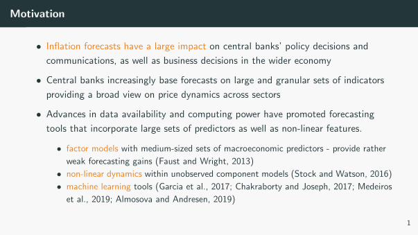
• Inflation forecasts have a large impact on central banks’ policy decisions and

communications, as well as business decisions in the wider economy

• Central banks increasingly base forecasts on large and granular sets of indicators

providing a broad view on price dynamics across sectors

• Advances in data availability and computing power have promoted forecasting

tools that incorporate large sets of predictors as well as non-linear features.

• factor models with medium-sized sets of macroeconomic predictors - provide rather

weak forecasting gains (Faust and Wright, 2013)

• non-linear dynamics within unobserved component models (Stock and Watson, 2016)

• machine learning tools (Garcia et al., 2017; Chakraborty and Joseph, 2017; Medeiros

et al., 2019; Almosova and Andresen, 2019)

1

What we do

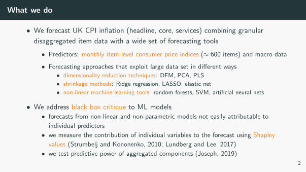
• We forecast UK CPI inflation (headline, core, services) combining granular

disaggregated item data with a wide set of forecasting tools

• Predictors: monthly item-level consumer price indices (≈ 600 items) and macro data

• Forecasting approaches that exploit large data set in different ways

• dimensionality reduction techniques: DFM, PCA, PLS

• shrinkage methods: Ridge regression, LASSO, elastic net

• non-linear machine learning tools: random forests, SVM, artificial neural nets

• We address black box critique to ML models• forecasts from non-linear and non-parametric models not easily attributable to

individual predictors

• we measure the contribution of individual variables to the forecast using Shapley

values (Strumbelj and Kononenko, 2010; Lundberg and Lee, 2017)

• we test predictive power of aggregated components (Joseph, 2019)

2

Key findings

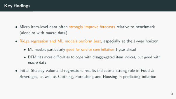
• Micro item-level data often strongly improve forecasts relative to benchmark

(alone or with macro data)

• Ridge regression and ML models perform best, especially at the 1-year horizon

• ML models particularly good for service core inflation 1-year ahead

• DFM has more difficulties to cope with disaggregated item indices, but good with

macro data

• Initial Shapley value and regressions results indicate a strong role in Food &

Beverages, as well as Clothing, Furnishing and Housing in predicting inflation

3

Where this fits in

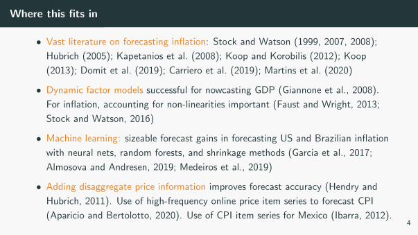
• Vast literature on forecasting inflation: Stock and Watson (1999, 2007, 2008);

Hubrich (2005); Kapetanios et al. (2008); Koop and Korobilis (2012); Koop

(2013); Domit et al. (2019); Carriero et al. (2019); Martins et al. (2020)

• Dynamic factor models successful for nowcasting GDP (Giannone et al., 2008).

For inflation, accounting for non-linearities important (Faust and Wright, 2013;

Stock and Watson, 2016)

• Machine learning: sizeable forecast gains in forecasting US and Brazilian inflation

with neural nets, random forests, and shrinkage methods (Garcia et al., 2017;

Almosova and Andresen, 2019; Medeiros et al., 2019)

• Adding disaggregate price information improves forecast accuracy (Hendry and

Hubrich, 2011). Use of high-frequency online price item series to forecast CPI

(Aparicio and Bertolotto, 2020). Use of CPI item series for Mexico (Ibarra, 2012).4

Data and forecasting setup

Setup

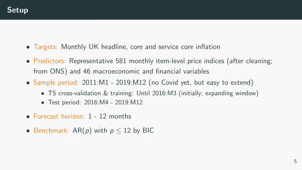
• Targets: Monthly UK headline, core and service core inflation

• Predictors: Representative 581 monthly item-level price indices (after cleaning;

from ONS) and 46 macroeconomic and financial variables

• Sample period: 2011:M1 - 2019:M12 (no Covid yet, but easy to extend)

• TS cross-validation & training: Until 2016:M3 (initially; expanding window)

• Test period: 2016:M4 - 2019:M12

• Forecast horizon: 1 - 12 months

• Benchmark: AR(p) with p ≤ 12 by BIC

5

CPI item series

• UK monthly CPI is constructed from about 700 representative item indices by theOffice for National Statistics (ONS), publically available

• Constructed by the ONS from single product prices collected in shops (price quotes)

• Item indices are weighted and aggregated into classes, groups, divisions, and finally

the CPI based on COICOP classification

• Our CPI item data set

• 581 item indices without missing values, 2011M1-2019M12

• items cover 84% of total CPI, similar coverage across broad CPI categories

• we use item indices in levels - ONS rebases and chain-links them to the January

value annually, which already removes trends from the series data

• indices are mean-variance standardised

• indices are seasonally adjusted - though a sub-set show additional spikes once a year

due to changes in weights. Could ML methods also deal with seasonality?

6

Forecasting models

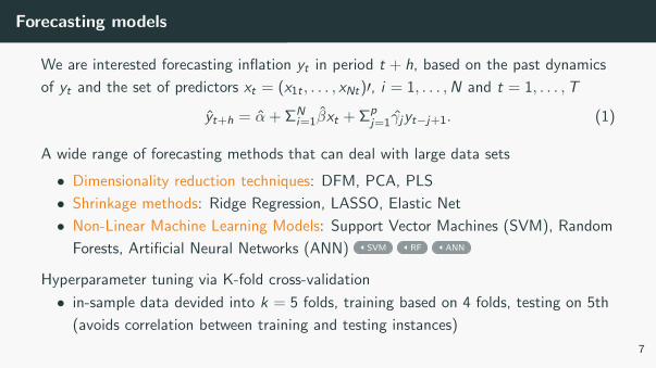
We are interested forecasting inflation yt in period t + h, based on the past dynamics

of yt and the set of predictors xt = (x1t , . . . , xNt)′, i = 1, . . . ,N and t = 1, . . . ,T

yt+h = α + ΣNi=1βxt + Σp

j=1γjyt−j+1. (1)

A wide range of forecasting methods that can deal with large data sets

• Dimensionality reduction techniques: DFM, PCA, PLS

• Shrinkage methods: Ridge Regression, LASSO, Elastic Net

• Non-Linear Machine Learning Models: Support Vector Machines (SVM), Random

Forests, Artificial Neural Networks (ANN) SVM RF ANN

Hyperparameter tuning via K-fold cross-validation

• in-sample data devided into k = 5 folds, training based on 4 folds, testing on 5th

(avoids correlation between training and testing instances)

7

Results

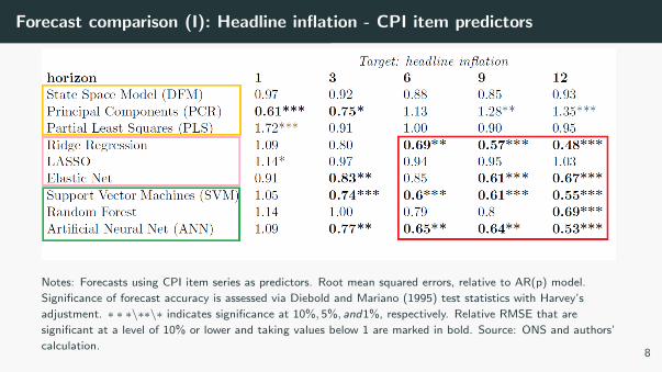
Forecast comparison (I): Headline inflation - CPI item predictors

Notes: Forecasts using CPI item series as predictors. Root mean squared errors, relative to AR(p) model.

Significance of forecast accuracy is assessed via Diebold and Mariano (1995) test statistics with Harvey’s

adjustment. ∗ ∗ ∗\∗∗\∗ indicates significance at 10%, 5%, and1%, respectively. Relative RMSE that are

significant at a level of 10% or lower and taking values below 1 are marked in bold. Source: ONS and authors’

calculation.8

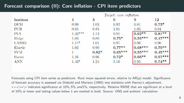
Forecast comparison (II): Core inflation - CPI item predictors

Forecasts using CPI item series as predictors. Root mean squared errors, relative to AR(p) model. Significance

of forecast accuracy is assessed via Diebold and Mariano (1995) test statistics with Harvey’s adjustment.

∗ ∗ ∗\∗∗\∗ indicates significance at 10%, 5%, and1%, respectively. Relative RMSE that are significant at a level

of 10% or lower and taking values below 1 are marked in bold. Source: ONS and authors’ calculation.

9

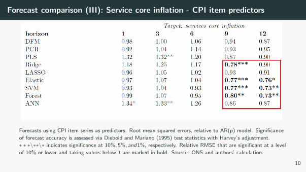
Forecast comparison (III): Service core inflation - CPI item predictors

Forecasts using CPI item series as predictors. Root mean squared errors, relative to AR(p) model. Significance

of forecast accuracy is assessed via Diebold and Mariano (1995) test statistics with Harvey’s adjustment.

∗ ∗ ∗\∗∗\∗ indicates significance at 10%, 5%, and1%, respectively. Relative RMSE that are significant at a level

of 10% or lower and taking values below 1 are marked in bold. Source: ONS and authors’ calculation.

10

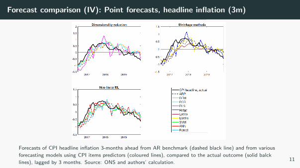
Forecast comparison (IV): Point forecasts, headline inflation (3m)

Forecasts of CPI headline inflation 3-months ahead from AR benchmark (dashed black line) and from various

forecasting models using CPI items predictors (coloured lines), compared to the actual outcome (solid balck

lines), lagged by 3 months. Source: ONS and authors’ calculation.11

Opening the black box of machine

learning [work in progress]

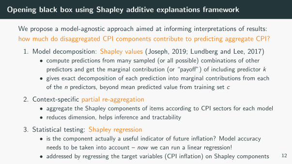
Opening black box using Shapley additive explanations framework

We propose a model-agnostic approach aimed at informing interpretations of results:

how much do disaggregated CPI components contribute to predicting aggregate CPI?

1. Model decomposition: Shapley values (Joseph, 2019; Lundberg and Lee, 2017)• compute predictions from many sampled (or all possible) combinations of other

predictors and get the marginal contribution (or “payoff”) of including predictor k

• gives exact decomposition of each prediction into marginal contributions from each

of the n predictors, beyond mean predicted value from training set c

2. Context-specific partial re-aggregation• aggregate the Shapley components of items according to CPI sectors for each model

• reduces dimension, helps inference and tractability

3. Statistical testing: Shapley regression• is the component actually a useful indicator of future inflation? Model accuracy

needs to be taken into account – now we can run a linear regression!

• addressed by regressing the target variables (CPI inflation) on Shapley components 12

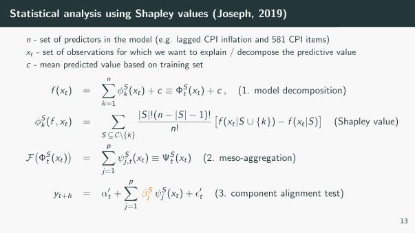
Statistical analysis using Shapley values (Joseph, 2019)

n - set of predictors in the model (e.g. lagged CPI inflation and 581 CPI items)

xt - set of observations for which we want to explain / decompose the predictive value

c - mean predicted value based on training set

f (xt) =n∑

k=1

φSk (xt) + c ≡ ΦSt (xt) + c , (1. model decomposition)

φSk (f , xt) =∑

S ⊆C\{k}

|S |!(n − |S | − 1)!

n!

[f (xt |S ∪ {k})− f (xt |S)

](Shapley value)

F(ΦSt (xt)

)=

p∑j=1

ψSj ,t(xt) ≡ ΨS

t (xt) (2. meso-aggregation)

yt+h = α′t +

p∑j=1

βSj ψSj (xt) + ε′t (3. component alignment test)

13

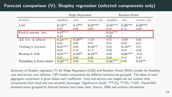
Forecast comparison (V): Shapley regression (selected components only)

Summary of Shapley regression (*) for Ridge Regression (LHS) and Random Forest (RHS) models for headline,

core and service core inflation. CPI models components for different horizons are grouped. The share of each

aggregate component is given below each coefficient. Core and service core targets do not contain item

components from food and non-alcoholic beverages. Significance levels: ***:1%, **:5%, *:10%. Panel-HAC

standard errors grouped by forecast horizon have been used. Source: ONS and authors calculations.

14

Take-away messages

• Micro-data are helpful to forecast macro outcomes

• Machine learning models deal well with high-dimensional datasets

• Ridge regression, SVMs and Random Forest show strong forecasting performance

9-12 months ahead

• Shapley values and regressions help to overcome the black box critique and allows

for standardised communication of results

15

Thanks for listening

contact: andreas.joseph@bankofengland.co.uk

16

References i

Almosova, A. and Andresen, N. (2019). Nonlinear inflation forecasting with recurrent neural networks. Unpublished manuscript.

Aparicio, D. and Bertolotto, M. I. (2020). Forecasting inflation with online prices. International Journal of Forecasting, 36(2):232–247.

Blake, A. P. and Kapetanios, G. (2000). A radial basis function artificial neural network test for arch. Economics Letters, 69(1):15–23.

Blake, A. P. and Kapetanios, G. (2010). Tests of the martingale difference hypothesis using boosting and rbf neural network approximations.

Econometric Theory, 26(5):1363–1397.

Carriero, A., Galvao, A. B., and Kapetanios, G. (2019). A comprehensive evaluation of macroeconomic forecasting methods. International Journal of

Forecasting, 35(4):1226–1239.

Chakraborty, C. and Joseph, A. (2017). Machine learning at central banks.

Diebold, F. X. and Mariano, R. S. (1995). Comparing predictive accuracy. Journal of Business and Economic Statistics, 13:253–263. Reprinted in

Mills, T. C. (ed.) (1999), Economic Forecasting. The International Library of Critical Writings in Economics. Cheltenham: Edward Elgar.

Domit, S., Monti, F., and Sokol, A. (2019). Forecasting the UK economy with a medium-scale Bayesian VAR. International Journal of Forecasting,

35(4):1669–1678.

Faust, J. and Wright, J. H. (2013). Forecasting inflation. In Handbook of economic forecasting, volume 2, pages 2–56. Elsevier.

Garcia, M. G., Medeiros, M. C., and Vasconcelos, G. F. (2017). Real-time inflation forecasting with high-dimensional models: The case of Brazil.

International Journal of Forecasting, 33(3):679–693.

Giannone, D., Reichlin, L., and Small, D. (2008). Nowcasting: The real-time informational content of macroeconomic data. Journal of Monetary

Economics, 55(4):665–676.

Hendry, D. F. and Hubrich, K. (2011). Combining disaggregate forecasts or combining disaggregate information to forecast an aggregate. Journal of

business & economic statistics, 29(2):216–227.

References ii

Hubrich, K. (2005). Forecasting euro area inflation: Does aggregating forecasts by hicp component improve forecast accuracy? International Journal

of Forecasting, 21(1):119–136.

Ibarra, R. (2012). Do disaggregated cpi data improve the accuracy of inflation forecasts? Economic Modelling, 29(4):1305–1313.

Joseph, A. (2019). Parametric inference with universal function approximators. Bank of England Staff Working Paper Series, (784).

Kapetanios, G., Labhard, V., and Price, S. (2008). Forecasting using bayesian and information-theoretic model averaging: an application to uk

inflation. Journal of Business & Economic Statistics, 26(1):33–41.

Koop, G. and Korobilis, D. (2012). Forecasting inflation using dynamic model averaging. International Economic Review, 53(3):867–886.

Koop, G. M. (2013). Forecasting with medium and large bayesian vars. Journal of Applied Econometrics, 28(2):177–203.

Lundberg, S. and Lee, S.-I. (2017). A Unified Approach to Interpreting Model Predictions. In Advances in Neural Information Processing Systems 30,

pages 4765–4774.

Martins, M. M., Verona, F., et al. (2020). Forecasting inflation with the new keynesian phillips curve: Frequency matters. Bank of Finland Research

Discussion Papers 4, 2020.

Medeiros, M. C., Vasconcelos, G. F., Veiga, A., and Zilberman, E. (2019). Forecasting inflation in a data-rich environment: the benefits of machine

learning methods. Journal of Business & Economic Statistics, pages 1–22.

Stock, J. H. and Watson, M. W. (1999). Forecasting inflation. Journal of Monetary Economics, 44(2):293–335.

Stock, J. H. and Watson, M. W. (2007). Why has US inflation become harder to forecast? Journal of Money, Credit and Banking, 39:3–33.

Stock, J. H. and Watson, M. W. (2008). Phillips curve inflation forecasts.

Stock, J. H. and Watson, M. W. (2016). Core inflation and trend inflation. Review of Economics and Statistics, 98(4):770–784.

References iii

Strumbelj, E. and Kononenko, I. (2010). An efficient explanation of individual classifications using game theory. Journal of Machine Learning

Research, 11:1–18.

Vapnik, V. (1998). Statistical learning theory. John Wiley&Sons Inc., New York.

Wang, Y., Wang, B., and Zhang, X. (2012). A new application of the support vector regression on the construction of financial conditions index to

cpi prediction. Procedia Computer Science, 9:1263–1272.

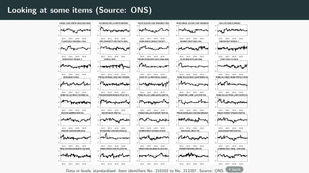
Looking at some items (Source: ONS)

2012 2014 2016 2018

-5

0

5

LARGE LOAF-WHITE-UNSLICED-800G

2012 2014 2016 2018

-5

0

5

SIX BREAD ROLLS-WHITE/BROWN

2012 2014 2016 2018

-5

0

5

WHITE SLICED LOAF BRANDED 750G

2012 2014 2016 2018

-5

0

5

WHOLEMEAL SLICED LOAF BRANDED

2012 2014 2016 2018

-5

0

5

CHILLED GARLIC BREAD

2012 2014 2016 2018

-5

0

5

FLOUR-SELF-RAISING-1.5KG

2012 2014 2016 2018

-5

0

5

DRY SPAGHETTI OR PASTA 500G

2012 2014 2016 2018

-5

0

5

CORN SNACK SINGLE PACKET

2012 2014 2016 2018

-5

0

5

BASMATI RICE 500G-1KG

2012 2014 2016 2018

-5

0

5

BREAKFAST CEREAL 1

2012 2014 2016 2018

-5

0

5

BREAKFAST CEREAL 2

2012 2014 2016 2018

-5

0

5

CEREAL BAR

2012 2014 2016 2018

-5

0

5

CREAM CRACKERS PACK 200G-300G

2012 2014 2016 2018

-5

0

5

PLAIN BISCUITS-200-300G

2012 2014 2016 2018

-5

0

5

FRUIT PIES 4-6 PACK

2012 2014 2016 2018

-5

0

5

DOUGHNUT-EACH

2012 2014 2016 2018

-5

0

5

WHOLE SPONGE CAKE NOT FROZEN

2012 2014 2016 2018

-5

0

5

PACK OF 5-6 INDIVIDUAL CAKES

2012 2014 2016 2018

-5

0

5

HOME KILLED BEEF-LEAN MINCE KG

2012 2014 2016 2018

-5

0

5

HOME KLD BEEF-RUMP/POPES STEAK

2012 2014 2016 2018

-5

0

5

HOME KILLED BEEF-TOPSIDE KG

2012 2014 2016 2018

-5

0

5

FROZEN BEEFBURGERS PACK OF 4

2012 2014 2016 2018

-5

0

5

HOME KILLED LAMB-SHOULDER KG

2012 2014 2016 2018

-5

0

5

FRZEN IMP LAMB: LEG (PER KG)

2012 2014 2016 2018

-5

0

5

HOME KILLED PORK-LOIN CHOPS KG

2012 2014 2016 2018

-5

0

5

BACON-GAMMON-PER KG

2012 2014 2016 2018

-5

0

5

BACON-BACK-PER KG

2012 2014 2016 2018

-5

0

5

FRESH/CHILLED CHICKEN PER KG

2012 2014 2016 2018

-5

0

5

FRESH BONELESS CHICKEN BREAST

2012 2014 2016 2018

-5

0

5

FRESH TURKEY STEAKS PER KG

2012 2014 2016 2018

-5

0

5

FROZEN CHICKEN BREASTS

2012 2014 2016 2018

-5

0

5

ROTISSERIE CHICKEN [WHOLE]

2012 2014 2016 2018

-5

0

5

CANNED MEAT-STEWED STEAK

2012 2014 2016 2018

-5

0

5

INDIVIDUAL MEAT PIE

2012 2014 2016 2018

-5

0

5

SAUSAGES-PORK-PER KG

2012 2014 2016 2018

-5

0

5

FROZ CHICKEN NUGGETS 220-600G

2012 2014 2016 2018

-5

0

5

FRESH WHITE FISH FILLETS KG

2012 2014 2016 2018

-5

0

5

FRESH FISH-SALMON FILLETS-KG

2012 2014 2016 2018

-5

0

5

FROZEN PRAWNS PER KG

2012 2014 2016 2018

-5

0

5

CANNED FISH, TUNA, 130G-200G

Data in levels, standardised. Item identifiers No. 210102 to No. 211207. Source: ONS. back

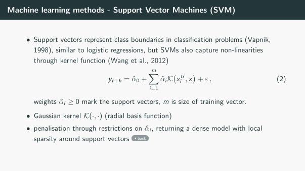
Machine learning methods - Support Vector Machines (SVM)

• Support vectors represent class boundaries in classification problems (Vapnik,

1998), similar to logistic regressions, but SVMs also capture non-linearities

through kernel function (Wang et al., 2012)

yt+h = α0 +m∑i=1

αiK(x tri , x

)+ ε , (2)

weights αi ≥ 0 mark the support vectors, m is size of training vector.

• Gaussian kernel K(·, ·) (radial basis function)

• penalisation through restrictions on αi , returning a dense model with local

sparsity around support vectors back

Machine learning methods - Random forests

• tree models consecutively split the training dataset until an assignment criterionwith respect to the target variable into a “data bucket” (leaf) is reached

• algorithm minimises objective function within “buckets”, conditioned on input xt• sparse models: only variables which actually improve the fit are chosen

The regression function is

yt+h =M∑

m=1

βmI(xt ∈ Pm) + εt , with βm = 1/|Pm|∑

y tr∈Pm

y tr , m ∈ {1, . . . ,M} .

(3)

• A random forest contains a set of uncorrelated trees which are estimatedseparately

• this overcomes overfitting of standard tree models

• but also harder to interpret due to the built-in randomness back

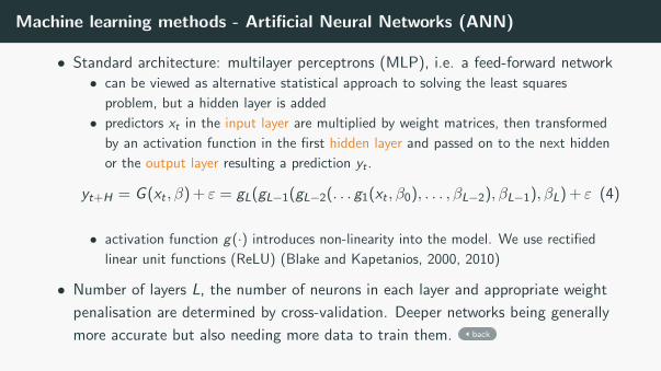
Machine learning methods - Artificial Neural Networks (ANN)

• Standard architecture: multilayer perceptrons (MLP), i.e. a feed-forward network• can be viewed as alternative statistical approach to solving the least squares

problem, but a hidden layer is added

• predictors xt in the input layer are multiplied by weight matrices, then transformed

by an activation function in the first hidden layer and passed on to the next hidden

or the output layer resulting a prediction yt .

yt+H = G (xt , β) + ε = gL(gL−1(gL−2(. . . g1(xt , β0), . . . , βL−2), βL−1), βL) + ε (4)

• activation function g(·) introduces non-linearity into the model. We use rectified

linear unit functions (ReLU) (Blake and Kapetanios, 2000, 2010)

• Number of layers L, the number of neurons in each layer and appropriate weight

penalisation are determined by cross-validation. Deeper networks being generally

more accurate but also needing more data to train them. back