Forecasting with Recurrent Neural Networks:12 Tricks

Hans-Georg Zimmermann, Christoph Tietz and Ralph Grothmann

Siemens AG, Corporate TechnologyOtto-Hahn-Ring 6, D-81739 Munich, Germany

Hans Georg.Zimmermann@siemens.com

Abstract. Recurrent neural networks (RNNs) are typically consideredas relatively simple architectures, which come along with complicatedlearning algorithms. This paper has a different view: We start from thefact that RNNs can model any high dimensional, nonlinear dynamicalsystem. Rather than focusing on learning algorithms, we concentrate onthe design of network architectures. Unfolding in time is a well-knownexample of this modeling philosophy. Here a temporal algorithm is trans-ferred into an architectural framework such that the learning can beperformed by an extension of standard error backpropagation.We introduce 12 tricks that not only provide deeper insights in the func-tioning of RNNs but also improve the identification of underlying dy-namical system from data.

1 Introduction

In many business management disciplines, complex planning and decision-makingcan be supported by quantitative forecast models that take into account a widerange of influencing factors with non-linear cause and effect relationships. Fur-thermore, the uncertainty in forecasting should be considered. The procurementof raw materials or demand planning are prime examples: The timing of copperpurchases can be optimized with accurate market price forecasts, whereas preciseforecasts of product sales increase the deliver reliability and reduce costs. Like-wise technical applications, e. g. energy generation, also require the modeling ofcomplex dynamical systems.

In this contribution we deal with time-delay recurrent neural networks (RNNs)for time series forecasting and introduce 12 tricks that not only ease the han-dling of RNNs, but also improve the forecast accuracy. The RNNs and associatedtricks are applied in many of our customer projects from economics and industry.

RNNs offer significant benefits for dealing with the typical challenges as-sociated with forecasting. With their universal approximation properties [11],RNNs can model high-dimensional, non-linear relationships. The time-delayedinformation processing addresses temporal structures. In contrast, conventionaleconometrics generally uses linear models (e.g. autoregressive models (AR), mul-tivariate linear regression) which can be efficiently estimated from historical data,but provide only an inadequate framework for non-linear dynamical systems [12].

2

In Section 2 we introduce the so-called correspondence principle for neuralnetworks (Trick 1). For us neural networks are a class of functions which can betransformed into architectures. We will work only with algorithms that processinformation locally within the architectures. As we will outline, for some prob-lems it is easier to start off with the NN architecture and formulate the equationsafterwards and for other problems vice versa. The locality of the algorithms en-ables us to model even large systems. The correspondence principle is the basisfor different RNN models and associated tricks.

We will start with a basic RNN in state space formulation for the modelingof partly autonomous and partly externally driven dynamical systems (so-calledopen systems). The associated parameter optimization task is solved by (finite)unfolding in time, which can be handled by a shared weights extension of stan-dard backpropagation. Dealing with state space models, we are able to utilizememory effects. Therefore, there is no need of a complicated input preprocess-ing in order to represent temporal relationships. Nevertheless, learning of opendynamical system tends to focus on the external drivers and, thus, neglects theidentification of the autonomous part. On this problem Trick 2 enforces the au-tonomous flow of the dynamics and thus, enables long-term forecasting. Trick 3finds a proper initialization for the first state vector of recurrent neural networkin the finite unfolding.

Typically we do not know all external drivers of the open dynamical system.This may cause the identification of pseudo causalities. Trick 4 is the extension ofthe RNN with an error correction term, resulting in a so-called error correctionneural network (ECNN), which enables us to handle missing information, hiddenexternal factors or shocks on the dynamics. ECNNs are an appropriate frame-work for low-dimensional dynamical systems with less than 5 target variables.For the modeling of high-dimensional systems on low dimensional manifolds asin electrical load curves Trick 5 adds a coordinate transformation (so-called bot-tleneck) to the ECNN.

Standard RNNs use external drivers in the past and assume constant envi-ronmental conditions from present time on. For fast changing environments thisis a questionable assumption. Internalizing the environment of the dynamicsinto the model, leads to Trick 6, so-called historically consistent neural networks(HCNN). The special feature of the HCNN is that it not only models the in-dividual dynamics of interest, but also models the external drivers. This leadsto a closed dynamical system formulation. Therefore, HCNNs are symmetric intheir input and output variables, i. e. the system description does not draw anydistinction between input, output and internal state variables.

In practice, HCNNs are difficult to train, because the models have no inputsignals and are unfolded across the complete data horizon. This implies that welearn from a single data pattern, which is the unique data history. In Trick 7 wetherefore introduce an architectural teacher forcing to make the best possibleuse of the data from the observables and to accelerate training of the HCNN.

The HCNN models the dynamics for all of the observables and their inter-action in parallel. For this purpose a high-dimensional state transition matrix is

3

required. A fully connected state transition matrix can, however, lead to a signaloverload during the training of the neural network using error backpropagationthrough time (EBTT). With Trick 8 we solve this problem by introducing sparsestate transition matrices.

The information flow within a HCNN is from the past to present and futuretime, i. e. we have a causal model to explain the highly-interacting non-lineardynamical systems across multiple time scales. Trick 9 extends this modelingframework with an information flow from the future into past. As we will showthis enables us to incorporate the effects of rational decision making and plan-ning into the modeling. The resulting models are called causal-retro-causal his-torically consistent neural networks (CRCNNs). Likewise to HCNNs, CRCNNsare difficult to train. In Trick 10 we extend the basic CRCNN architecture by anarchitectural teacher forcing mechanism, which allows us to learn the CRCNNusing the standard EBTT algorithm. Trick 11 introduces a way to improve themodeling of deterministic chaotic systems.

Finally, Trick 12 is dedicated to the modeling of uncertainty and risk. Wecalculate ensembles of either HCNNs or CRCNNs to forecast probability distri-butions. Both modeling frameworks give a perfect description of the dynamicof the observables in the past. However, the partial observability of the worldresults in a non-unique reconstruction of the hidden variables and thus, differentfuture scenarios. Since the genuine development of the dynamics is unknownand all paths have the same probability, the average of the ensemble is the bestforecast, whereas the ensemble bandwidth describes the market risk.

Section 3 summarizes the primary findings of this contribution and points tofuture directions of research.

2 Tricks for Recurrent Neural Networks

Trick 1. The Correspondence Principle for Neural Networks

In order to gain a deeper understanding in the functioning and composition ofRNNs we introduce our first conceptual trick, which is called correspondenceprinciple between equations, architectures and local algorithms. The correspon-dence principle for neural networks (NN) implies that any equation for a NN canbe portrayed in graphical form by means of an architecture which represents theindividual layers of the network in the form of nodes and the matrices betweenthe layers in the form of edges. This correspondence is most beneficial in combi-nation with local optimization algorithms that provide the basis for the trainingof the NNs. For example, the error back propagation algorithm needs only lo-cally available information from the forward and backward flow of the networkin order to calculate the partial derivatives of the NN error function[13]. Theuse of local algorithms here provides an elegant basis for the expansion of theneural network towards the modeling of large systems. Used in combination withan appropriate (stochastic) learning rule, it is possible to use the gradients as abasis for the identification of robust minima[8].

4

Now let us introduce a basic recurrent neural network (RNN) in state spaceformulation. We start from the assumption that a vector time series yτ is createdby an open dynamical system, which can be described in discrete time τ usinga state transition and output equation[3]:

state transition sτ+1 = f(sτ , uτ )output equation yτ = g(sτ )

(1)

The hidden time-recurrent state transition equation sτ+1 = f(sτ , uτ ) describesthe upcoming state sτ+1 by means of a function of the current system state sτand of the external factors uτ . The system formulated in the state transitionequation can therefore be interpreted as a partially autonomous and partiallyexternally driven dynamic. We call this an open dynamical system.

The output, also called observer, equation yτ uses the non-observable systemstate sτ in every time step τ to calculate the output of the dynamic systemyτ . The data-driven system identification is based on the selected parameterizedfunctions f() and g(). We chose the parameters in f() and g() such that anappropriate error function is minimized (see Eq. 2).

1

T

T∑τ=1

(yτ − ydτ

)2 → minf,g

. (2)

The two functions f() and g() are estimated using the quadratic error function(Eq. 2) in such a way that the average distance between the observed data ydτ andthe system outputs yτ across a number of observations τ = 1, . . . , T is minimal.

Thus far, we have given a general description of the state transition andthe output equation for open dynamical systems. Without loss of generality wecan specify the functions f() and g() by means of a recurrent neural network(RNN)[11, 15]:

state transition sτ+1 = tanh(Asτ +Buτ )output equation yτ = Csτ

(3)

Eq. 3 specifies an RNN with weight matrices A, B and C to model the open dy-namical system. The RNN is designed as a non-linear state-space model, whichis able to approximate any function f() and g(). We choose the hyperbolic tan-gent tanh() as the activation function for the hidden network layer sτ+1. Theoutput equation is specified as a linear function. The RNN output is generatedby a superposition of two components: (i) the autonomous dynamics (coded inA), which accumulates information over time (memory), and (ii) the influenceof external factors (coded in B).

Note, that the state transition in Eq. 3 does not need an additional matrixleading the hyperbolic tangent tanh() activation function, since the additionalmatrix can be merged into matrix A. Furthermore, without loss of generality wecan use a linear output equation in Eq. 3. If we would have a non-linearity inthe output equation (Eq. 3), it could be merged in the state transition equation(Eq. 3). For details see Schafer et al. [11].

5

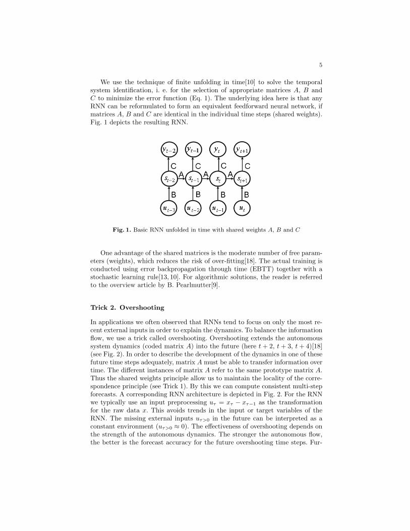
We use the technique of finite unfolding in time[10] to solve the temporalsystem identification, i. e. for the selection of appropriate matrices A, B andC to minimize the error function (Eq. 1). The underlying idea here is that anyRNN can be reformulated to form an equivalent feedforward neural network, ifmatrices A, B and C are identical in the individual time steps (shared weights).Fig. 1 depicts the resulting RNN.

Fig. 1. Basic RNN unfolded in time with shared weights A, B and C

One advantage of the shared matrices is the moderate number of free param-eters (weights), which reduces the risk of over-fitting[18]. The actual training isconducted using error backpropagation through time (EBTT) together with astochastic learning rule[13, 10]. For algorithmic solutions, the reader is referredto the overview article by B. Pearlmutter[9].

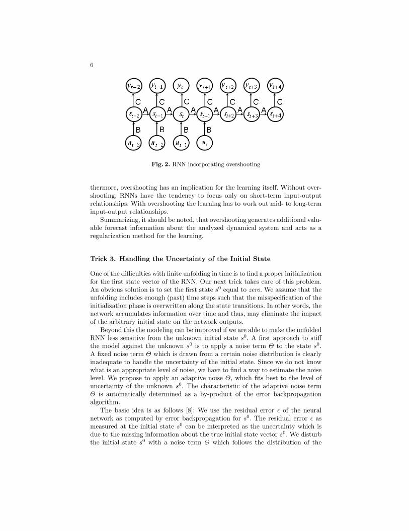
Trick 2. Overshooting

In applications we often observed that RNNs tend to focus on only the most re-cent external inputs in order to explain the dynamics. To balance the informationflow, we use a trick called overshooting. Overshooting extends the autonomoussystem dynamics (coded matrix A) into the future (here t + 2, t + 3, t + 4)[18](see Fig. 2). In order to describe the development of the dynamics in one of thesefuture time steps adequately, matrix A must be able to transfer information overtime. The different instances of matrix A refer to the same prototype matrix A.Thus the shared weights principle allow us to maintain the locality of the corre-spondence principle (see Trick 1). By this we can compute consistent multi-stepforecasts. A corresponding RNN architecture is depicted in Fig. 2. For the RNNwe typically use an input preprocessing uτ = xτ − xτ−1 as the transformationfor the raw data x. This avoids trends in the input or target variables of theRNN. The missing external inputs uτ>0 in the future can be interpreted as aconstant environment (uτ>0 ≈ 0). The effectiveness of overshooting depends onthe strength of the autonomous dynamics. The stronger the autonomous flow,the better is the forecast accuracy for the future overshooting time steps. Fur-

6

Fig. 2. RNN incorporating overshooting

thermore, overshooting has an implication for the learning itself. Without over-shooting, RNNs have the tendency to focus only on short-term input-outputrelationships. With overshooting the learning has to work out mid- to long-terminput-output relationships.

Summarizing, it should be noted, that overshooting generates additional valu-able forecast information about the analyzed dynamical system and acts as aregularization method for the learning.

Trick 3. Handling the Uncertainty of the Initial State

One of the difficulties with finite unfolding in time is to find a proper initializationfor the first state vector of the RNN. Our next trick takes care of this problem.An obvious solution is to set the first state s0 equal to zero. We assume that theunfolding includes enough (past) time steps such that the misspecification of theinitialization phase is overwritten along the state transitions. In other words, thenetwork accumulates information over time and thus, may eliminate the impactof the arbitrary initial state on the network outputs.

Beyond this the modeling can be improved if we are able to make the unfoldedRNN less sensitive from the unknown initial state s0. A first approach to stiffthe model against the unknown s0 is to apply a noise term Θ to the state s0.A fixed noise term Θ which is drawn from a certain noise distribution is clearlyinadequate to handle the uncertainty of the initial state. Since we do not knowwhat is an appropriate level of noise, we have to find a way to estimate the noiselevel. We propose to apply an adaptive noise Θ, which fits best to the level ofuncertainty of the unknown s0. The characteristic of the adaptive noise termΘ is automatically determined as a by-product of the error backpropagationalgorithm.

The basic idea is as follows [8]: We use the residual error ε of the neuralnetwork as computed by error backpropagation for s0. The residual error ε asmeasured at the initial state s0 can be interpreted as the uncertainty which isdue to the missing information about the true initial state vector s0. We disturbthe initial state s0 with a noise term Θ which follows the distribution of the

7

residual error ε. Given the uncertain initial states, learning tries to fulfill theoutput-target relationships along the dynamics. As a result of the learning weget a state transition matrix in form of a contraction, which squeezes out theinitial uncertainty. A corresponding network architecture is depicted in Fig. 3.

Fig. 3. Handling the uncertainty of the initial state s0 by applying adaptive noise.

It is important to notice, that the noise term Θ is drawn from the observedresidual errors without any assumption on the underlying noise distribution. Thedesensitization of the network to the initial state vector s0 can therefore be seenas a self-scaling stabilizer of the modeling.

In general, a time discrete trajectory can be seen as a sequence of pointsover time. Such a trajectory is comparable to a fine thread in the internal statespace. The trajectory is very sensitive to the initial state vector s0. If we applynoise to s0, the trajectory becomes a tube in the internal state space. Due tothe characteristics of the adaptive noise term, the tube contracts over time. Thisenforces the identification of a stable dynamical system.

Trick 4. Error Correction Neural Networks (ECNN)

A weakness of the RNN (see Fig. 1 or 2) is, that modeling might be disturbedby unknown external influences or shocks. As a remedy, the next trick callederror correction neural networks (ECNN) introduces an additional term zτ =tanh(yτ − ydτ ) in the state transition (4). The term can be interpreted as ancorrectional factor: The model error (yτ −ydτ ) at time τ quantifies the misfit andmay help to adjust the model output afterwards.

state transition sτ+1 = tanh(Asτ +Buτ +D tanh(yτ − ydτ ))output equation yτ = Csτ

(4)

In Eq. 4 the model output yτ is computed by Csτ and compared with theobservation ydτ . The output clusters of the ECNN which generate error signals

8

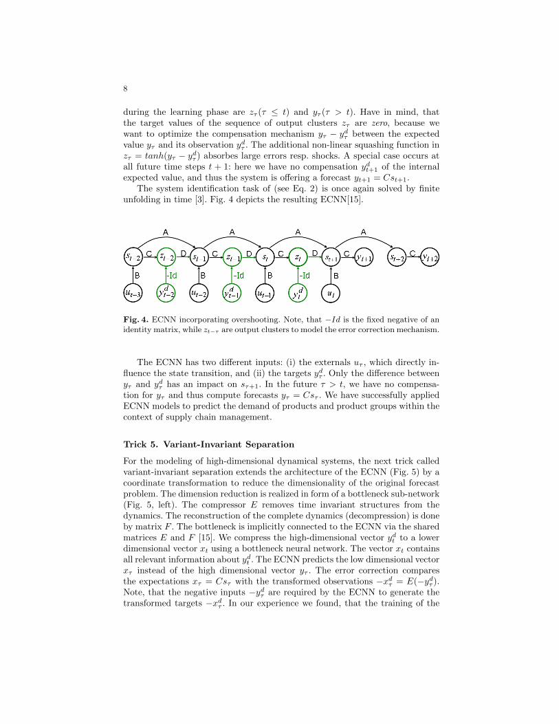
during the learning phase are zτ (τ ≤ t) and yτ (τ > t). Have in mind, thatthe target values of the sequence of output clusters zτ are zero, because wewant to optimize the compensation mechanism yτ − ydτ between the expectedvalue yτ and its observation ydτ . The additional non-linear squashing function inzτ = tanh(yτ − ydτ ) absorbes large errors resp. shocks. A special case occurs atall future time steps t + 1: here we have no compensation ydt+1 of the internalexpected value, and thus the system is offering a forecast yt+1 = Cst+1.

The system identification task of (see Eq. 2) is once again solved by finiteunfolding in time [3]. Fig. 4 depicts the resulting ECNN[15].

Fig. 4. ECNN incorporating overshooting. Note, that −Id is the fixed negative of anidentity matrix, while zt−τ are output clusters to model the error correction mechanism.

The ECNN has two different inputs: (i) the externals uτ , which directly in-fluence the state transition, and (ii) the targets ydτ . Only the difference betweenyτ and ydτ has an impact on sτ+1. In the future τ > t, we have no compensa-tion for yτ and thus compute forecasts yτ = Csτ . We have successfully appliedECNN models to predict the demand of products and product groups within thecontext of supply chain management.

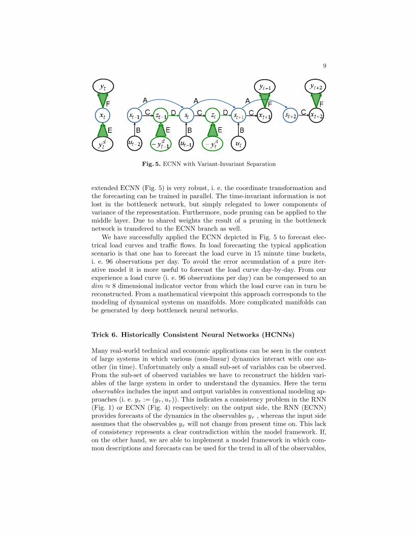
Trick 5. Variant-Invariant Separation

For the modeling of high-dimensional dynamical systems, the next trick calledvariant-invariant separation extends the architecture of the ECNN (Fig. 5) by acoordinate transformation to reduce the dimensionality of the original forecastproblem. The dimension reduction is realized in form of a bottleneck sub-network(Fig. 5, left). The compressor E removes time invariant structures from thedynamics. The reconstruction of the complete dynamics (decompression) is doneby matrix F . The bottleneck is implicitly connected to the ECNN via the sharedmatrices E and F [15]. We compress the high-dimensional vector ydt to a lowerdimensional vector xt using a bottleneck neural network. The vector xt containsall relevant information about ydt . The ECNN predicts the low dimensional vectorxτ instead of the high dimensional vector yτ . The error correction comparesthe expectations xτ = Csτ with the transformed observations −xdτ = E(−ydτ ).Note, that the negative inputs −ydτ are required by the ECNN to generate thetransformed targets −xdτ . In our experience we found, that the training of the

9

Fig. 5. ECNN with Variant-Invariant Separation

extended ECNN (Fig. 5) is very robust, i. e. the coordinate transformation andthe forecasting can be trained in parallel. The time-invariant information is notlost in the bottleneck network, but simply relegated to lower components ofvariance of the representation. Furthermore, node pruning can be applied to themiddle layer. Due to shared weights the result of a pruning in the bottlenecknetwork is transfered to the ECNN branch as well.

We have successfully applied the ECNN depicted in Fig. 5 to forecast elec-trical load curves and traffic flows. In load forecasting the typical applicationscenario is that one has to forecast the load curve in 15 minute time buckets,i. e. 96 observations per day. To avoid the error accumulation of a pure iter-ative model it is more useful to forecast the load curve day-by-day. From ourexperience a load curve (i. e. 96 observations per day) can be compressed to andim ≈ 8 dimensional indicator vector from which the load curve can in turn bereconstructed. From a mathematical viewpoint this approach corresponds to themodeling of dynamical systems on manifolds. More complicated manifolds canbe generated by deep bottleneck neural networks.

Trick 6. Historically Consistent Neural Networks (HCNNs)

Many real-world technical and economic applications can be seen in the contextof large systems in which various (non-linear) dynamics interact with one an-other (in time). Unfortunately only a small sub-set of variables can be observed.From the sub-set of observed variables we have to reconstruct the hidden vari-ables of the large system in order to understand the dynamics. Here the termobservables includes the input and output variables in conventional modeling ap-proaches (i. e. yτ := (yτ , uτ )). This indicates a consistency problem in the RNN(Fig. 1) or ECNN (Fig. 4) respectively: on the output side, the RNN (ECNN)provides forecasts of the dynamics in the observables yτ , whereas the input sideassumes that the observables yτ will not change from present time on. This lackof consistency represents a clear contradiction within the model framework. If,on the other hand, we are able to implement a model framework in which com-mon descriptions and forecasts can be used for the trend in all of the observables,

10

we will be in a position to close the open system - in other words, we will modela closed large dynamic system.

The next trick called historically consistent neural networks (HCNNs) in-troduces a model class which follows the design principles for modeling of largedynamic systems and overcomes the conceptual weaknesses of conventional mod-els. Equation 5 formulates the historically consistent neural network (HCNN).

state transition sτ+1 = A tanh(sτ )output equation yτ = [Id, 0]sτ

(5)

The joint dynamics for all observables is characterized in the HCNN (5) bythe sequence of states sτ . The observables (i = 1, . . . , N) are arranged on thefirst N state neurons sτ and followed by non-observable (hidden) variables assubsequent neurons. The connector [Id, 0] is a fixed matrix which reads out theobservables. The initial state s0 is described as a bias vector. The bias s0 andmatrix A contain the only free parameters.

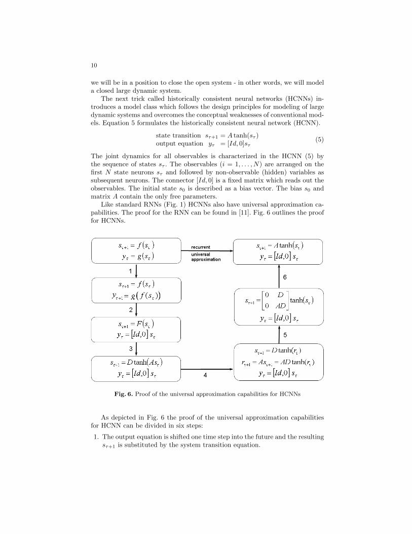
Like standard RNNs (Fig. 1) HCNNs also have universal approximation ca-pabilities. The proof for the RNN can be found in [11]. Fig. 6 outlines the prooffor HCNNs.

Fig. 6. Proof of the universal approximation capabilities for HCNNs

As depicted in Fig. 6 the proof of the universal approximation capabilitiesfor HCNN can be divided in six steps:

1. The output equation is shifted one time step into the future and the resultingsτ+1 is substituted by the system transition equation.

11

2. By combining outputs and state variables into an extended state we get anextended state transition equation. The output of the system is derived fromthe first components of the extended internal state.

3. For the extended state transition equation we apply the feedforward univer-sal approximation theorem. At least for a finite time horizon this guaranteesa small approximation error. Note, that in RNNs at least one large compo-nent of the state vector together with the hyperbolic tangent can mimic abias vector. Thus, we have omitted the explicit notation of a bias vector inthe NN equations.

4. In this step we remove one of the two matrices within the state transitionequation. We apply a state transformation rτ = Asτ . This results in twostate transition equations.

5. The two state transition equations can be reorganized in one state transition,which has twice the dimensionality of the original equation.

6. Rewriting the matrix located on front of the tanh activation function resultsin the claimed formulation for closed systems.

Instead of being applied inside the tanh activation function, matrix A is usedoutside the tanh activation function. This has the advantage that the states andthus, also the system outputs are not limited to the finite state space (−1; 1)n

created by the tanh(.) nonlinearity. The output equation has a simple and ap-plication independent form. Note, that we can only observe the first elements ofthe state vector.

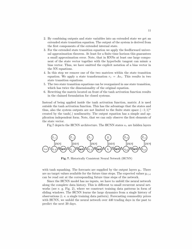
Fig.7 depicts the HCNN architecture. The HCNN states sτ are hidden layers

Fig. 7. Historically Consistent Neural Network (HCNN)

with tanh squashing. The forecasts are supplied by the output layers yτ . Thereare no target values available for the future time steps. The expected values yτ>tcan be read out at the corresponding future time steps of the network.

Since the HCNN model has no inputs, we have to unfold the neural networkalong the complete data history. This is different to small recurrent neural net-works (see e. g. Fig. 2), where we construct training data patterns in form ofsliding windows. The HCNN learns the large dynamics from a single history ofobservations (i. e. a single training data pattern). Forecasting commodity priceswith HCNN, we unfold the neural network over 440 trading days in the past topredict the next 20 days.

12

Trick 7. Architectural Teacher Forcing (ATF) for HCNNs

In practice we observe that HCNNs are difficult to train since the models do nothave any input signals and are unfolded across the complete data set. Our nexttrick, architectural teacher forcing (ATF) for HCNNs, makes the best possibleuse of the data from the observables and accelerates the training of the HCNN[20, 14, 9]. The HCNN with integrated teacher forcing is shown in Fig. 8 below.In the HCNN with ATF (Fig. 8) the expected values for all observables up to

Fig. 8. HCNN with Architectural Teacher Forcing (ATF)

time τ = t are replaced with the actual observations. The output layers of theHCNN are given fixed target values of zero. The negative observed values −ydτfor the observables are added to the output layer. This forces the HCNN tocreate the expected values yτ to compensate for the negative observed values−ydτ . The content of the output layer, i. e. yτ − ydτ , is now transferred to thefirst N neurons of the hidden layer rτ on a component-by-component basis witha minus symbol. In addition, we copy the expected values yτ from the state sτto the intermediate hidden layer rτ . As a result, the expected values yτ on thefirst N components of the state vector sτ are replaced by the observed valuesydτ = yτ − (yτ − ydτ ) (Fig. 8). All connections of the ATF mechanism are fixed.Following the ATF step, the state transition matrix A is applied, to move thesystem into the next time step. By definition, we have no observations for theobservables in future time steps. Here, the system is iterated exclusively upon theexpected values. This turns an open into a closed dynamic system. The HCNNin Fig. 8 is equivalent to the architecture in Fig.7, if it converges to zero errorin the training. In this case we have solved the original problem.

Trick 8. Sparsity, Dimensionality vs. Connectivity and Memory

HCNNs may have to model ten, twenty or even more observables in parallelover time. It is clear that we have to work with high dimensional dynamicalsystems (e. g. in our commodity price models we use dim(s) = 300). The iterationwith a fully connected state transition matrix A of such a dimension is dangerous:Sometimes the matrix vector operations will produce large numbers which willbe spread in the recursive computation all over the network and will generate

13

an arithmetic overflow. To avoid this phenomena we can choose a sparse matrixA. Thus, the linear algebra does not accumulate large numbers and the spreadof large numbers through the network is damped by the sparsity too.

We have to answer the questions which dimensionality and which sparsitywe will choose. In [16] we have worked out that dimensionality and sparsityare related to another pair of meta-parameters: Connectivity (con) and memorylength (mem). Connectivity is defined as the number of nonzero elements ineach row of matrix A. The memory length is the number of steps from whichwe have to collect information in order to reach a Markovian state, i. e. thestate vector contains all necessary information from the past. We propose thefollowing parameterization for the state dimension (dim(s)) and sparsity [16]:

Dimension of A dim(s) = con ·mem (6)

Sparsity of A Sparsity = random( con

mem · con

)= random

(1

mem

)(7)

Eq. 7 represents the insight that a sparse system conserves information over alonger time period before it diffuses in the network. For instance a shift registeris very sparse and behaves only as a memory, whereas in a fully connected matrixthe superposition of information masks the information sources. Let us assumethat we have initialized the state transition matrix with a uniformm randomsparse matrix A. Following Eq. 7 the more dense parts of A will model the fastersub-dynamics within the overall dynamics, while the highly sparse parts of Awill focus on slow subsystems. As a result a sparse random initialization allowsthe combined modeling of systems on different time scales.

Unfortunately, Eq. 6 favors very large dimensions. Our earlier work on thesubject (see [16]) started with the predefinition of the systems memory lengthmem, because for RNNs the memory length is equal to the length of the pastunfolding in time. On the other hand, connectivity has to be chosen larger thanthe number of the observables. Working with HCNNs the memory length is lessimportant, because we unfold the neural network along the whole data horizon.Here the connectivity plays the superior role. From our experience we know thatthe EBTT algorithm works stably with a connectivity which is equal or smallerthan 50 (con ≤ 50). For computational performance we usually limit the statedimensionality to dim(s) = 300. This implies a sparsity of 50/300 ≈ 17%. Weleave the fine tuning of the parameters to the EBTT learning.

We propose to initialize the neural network with a randomly chosen spar-sity grid. The sparsity grid is therefore chosen arbitrary and not optimized bye. g. pruning algorithms. This raises the question if a random sparse initializa-tion biases the network towards inferior solutions. This is handled by ensembleforecasts. We have performed ensemble experiments with different sparsity gridsversus ensembles based on the same sparsity grid. We found, that the average ofthe ensemble as well as the ensemble width are unaffected by the initialization ofthe sparsity grid (for more details on ensemble forecasting see Trick 12). Theseconsiderations hold only for large systems.

14

Trick 9. Causal-Retro-Causal Neural Networks (CRCNNs)

The fundamental idea of the HCNN is to explain the joint dynamics of theobservables in a causal manner, i. e. with an information flow from the pastto the future. However, rational planning is not only a consequence of a causalinformation flow but also of anticipating future developments and respondingto them on the basis of a certain goal function. This is similar to the adjointequation in optimal control theory [6]. In other words a retro causal informationflow is equivalent to asking for the motivation of a behavior as a goal. In turn,this is the anchor point for the reconstruction of the dynamics.

In order to incorporate the effects of rational decision making and planninginto the modeling, the next trick introduces causal-retro-causal neural networks(CRCNNs). The idea behind the CRCNN is to enrich the causal informationflow within the HCNN, which is directed from the past to the future, by a retro-causal information flow, directed from the future into the past. The CRCNNmodel is given by the following set of equations 8.

causal state transition sτ = A tanh(sτ−1)retro-causal state transition s′τ = A′ tanh(s′τ+1)output equation yτ = [Id, 0]sτ + [Id, 0]s′τ .

(8)

The output equation yτ of the CRCNN (Eq. 8) is a mixture of causal and retro-causal influences. The dynamics of all observables is hence explained by a se-quence of causal (sτ ) and retro-causal states s′τ using transition matrices A andA′ for the causal and retro-causal information flow. Upon the basis of Eq. 8, wedraw the network architecture for the CRCNN as depicted in Fig. 9.

Fig. 9. A Causal-Retro-Causal Historically Consistent Neural Network (CRCNN)

Trick 10. Architectural Teacher Forcing (ATF) for CRCNNs

The CRCNN (Fig. 9) is also unfolded across the entire time path, i. e. we learnthe unique history of the system. Likewise to the training of the HCNN, CRCNNsare difficult to train. Our next trick called architectural teacher forcing (ATF)for CRCNNs formulates TF as a part of the CRCNN architecture, which allows

15

us to learn the CRCNN using the standard EBTT algorithm[3]. ATF enables usto exploit the information contained in the data more efficiently and acceleratesthe training itself. Fig. 10 depicts the CRCNN architecture incorporating ATF.

Fig. 10. Extended CRCNN with an architectural Teacher Forcing (ATF) mechanism

Let us explain the ATF mechanism in the extended CRCNN model (Fig. 10):The extended CRCNN uses a causal-retro-causal network to correct the errorof the opposite part of the network in a symmetric manner. In every time stepτ ≤ t the expected values yτ are replaced by the observations ydτ using theintermediate tanh() layers for the causal and for the retro-causal part. Sincethe causal and the retro-causal part jointly explain the observables yτ , we haveto inject the causal into the retro-causal part and vice versa. This is done bycompensating the actual observations −ydτ with the output of the causal (∆τ )and the retro-causal part (∆′τ ) within output layers with fixed target values ofzero. The resulting content (∆τ+∆′τ−ydτ = 0) of the output layers is negated andtransferred to the causal and retro-causal part of the CRCNN using the fixed[−Id, 0]′ connector. Within the intermediate tanh() layers the expectations ofyτ are replaced with the actual observations ydτ , whereby the contribution to yτfrom the opposite part of the CRCNN is considered. Note, that ATF does notlead to a larger number of free network parameters, since all new connectionsare fixed and are used only to transfer data in the NN. In future direction τ > tthe CRCNN is iterated exclusively on the basis of expected values.

The usage of ATF does not reintroduce an input / output modeling, since wereplace the expected value of the observables with their actual observations, whilesimultaneously considering the causal and retro-causal part of the dynamics.For sufficiently large CRCNNs and convergence of the output error to zero, thearchitecture in Fig. 10 converges towards the fundamental CRCNN architectureshown in Fig. 9. The advantage of the CRCNN is, that it allows a fully dynamicalsuperposition of the causal and retro-causal information flows.

The CRCNN depicted in Fig. 10 describes a dynamics on a manifold. Inevery time step the information flows incorporates closed loops, which technically

16

can be seen as equality constraints. These contraints are only implicitly definedthrough the interaction of the causal and retro-causal parts. The closed loopsin the CRCNN architecture (Fig. 10) lead to fix-point recurrent substructureswithin the model, which are hard to handle with EBTT. As a remedy we proposea solution concept similar to Trick 7: We embedd the CRCNN model into a largernetwork architecture, which is easier to solve and converges to the same solutionas the original system. Fig. 11 depicts an initial draft for such an embedding.

Fig. 11. Asymmetric split of ATF in CRC neural networks

The extended architecture in Fig. 11 is a duplication of the origonal modeldepicted in Fig. 10. The CRCNN architecture in Fig. 11 does not contain closedloops, because we splitted the ATF mechanism for the causal and retro-causalpart into two branches. It is important to notices that these branches are implic-itly connected through the shared weights in the causal and retro-causal part.If this architecture converges, the ATF is no longer required and we have twoidentical copies of the CRCNN model depicted in Fig. 9. The solution proposedfor the embedding is not the only feasible way to handle the fix-point loops. Wewill outline alternative solutions in an upcomming paper. The CRCNN is thebasis for our projects on forecasting commodity prices.

Trick 11. Stable & Instable Information Flows in Dynamical Systems

Following Trick 3 it is natural to apply noise in the causal as well as in retro-causal branch (see also Fig. 12). This should improve the stability of both timedirections resp. information flows. In CRCNNs this feature has a special inter-pretation: Stability in the causal information flow means that the uncertainty

17

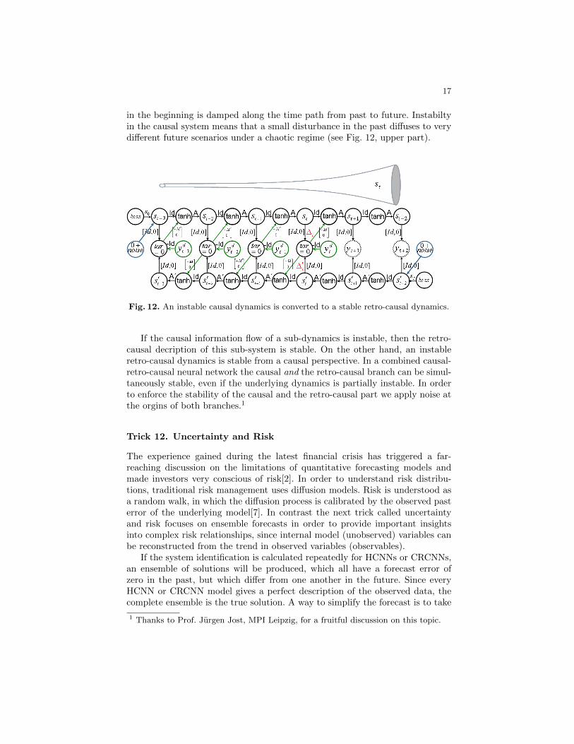
in the beginning is damped along the time path from past to future. Instabiltyin the causal system means that a small disturbance in the past diffuses to verydifferent future scenarios under a chaotic regime (see Fig. 12, upper part).

Fig. 12. An instable causal dynamics is converted to a stable retro-causal dynamics.

If the causal information flow of a sub-dynamics is instable, then the retro-causal decription of this sub-system is stable. On the other hand, an instableretro-causal dynamics is stable from a causal perspective. In a combined causal-retro-causal neural network the causal and the retro-causal branch can be simul-taneously stable, even if the underlying dynamics is partially instable. In orderto enforce the stability of the causal and the retro-causal part we apply noise atthe orgins of both branches.1

Trick 12. Uncertainty and Risk

The experience gained during the latest financial crisis has triggered a far-reaching discussion on the limitations of quantitative forecasting models andmade investors very conscious of risk[2]. In order to understand risk distribu-tions, traditional risk management uses diffusion models. Risk is understood asa random walk, in which the diffusion process is calibrated by the observed pasterror of the underlying model[7]. In contrast the next trick called uncertaintyand risk focuses on ensemble forecasts in order to provide important insightsinto complex risk relationships, since internal model (unobserved) variables canbe reconstructed from the trend in observed variables (observables).

If the system identification is calculated repeatedly for HCNNs or CRCNNs,an ensemble of solutions will be produced, which all have a forecast error ofzero in the past, but which differ from one another in the future. Since everyHCNN or CRCNN model gives a perfect description of the observed data, thecomplete ensemble is the true solution. A way to simplify the forecast is to take

1 Thanks to Prof. Jurgen Jost, MPI Leipzig, for a fruitful discussion on this topic.

18

the arithmetical average of the individual ensemble members as the expectedvalue, provided the ensemble histogram is unimodal in every time step.

In addition to the expected value, we consider the bandwidth of the ensem-ble, i. e. its distribution. The form of the ensemble is governed by differencesin the reconstruction of the hidden system variables from the observables: forevery finite volume of observations there is an infinite number of explanationmodels which describe the data perfectly, but differ in their forecasts, since theobservations make it possible to reconstruct the hidden variables in differentforms during the training. In other words, our risk concept is based on the par-tial observability of the world, leading to different reconstructions of the hiddenvariables and thus, different future scenarios. Since all scenarios are perfectlyconsistent with the history, we do not know which of the scenarios describes thefuture trend best and risk emerges.

This approach directly addresses the model risk. For HCNN and CRCNNmodeling we claim that the model risk is equal to the forecast risk. The reasonscan be summarized as follows: First, HCNNs are universal approximators, whichare therefore able to describe every market scenario. Second, the form of theensemble distribution is caused by an underlying dynamics, which interpret themarket dynamics as the result of interacting decisions[17]. Third, in experimentswe have shown that the ensemble distribution is independent from the details ofthe model configuration, if we use large models and large ensembles.

Let us exemplify our risk concept. The diagram below (Fig. 13, left) showsthe approach applied to the Dow Jones Industrial Index (DJX). For the ensem-ble, a HCNN was used to generate 250 individual forecasts for the DJX. For

Fig. 13. HCNN ensemble forecast for the Dow Jones Index (12 weeks forecast horizon),left, and associated index point distribution for the ensemble in time step t+ 12, right.

every forecast date, all of the individual forecasts for the ensemble represent theempirical density function, i. e. a probability distribution over many possiblemarket prices at a single point in time (see Fig. 13, right). It is noticeable thatthe actual development of the DJX is always within the ensemble channel (seegray lines, Fig. 13, left). The expected value for the forecast distribution is alsoan adequate point forecast for the DJX (see Fig. 13, right).

19

3 Conclusion and Outlook

Recurrent neural networks model dynamical systems in the form of non-linearstate space models. Just like any other NN, the equation of the RNNs, ECNNs,HCNNs or CRCNNs can be expressed as an architecture which represents theindividual layers in the form of nodes and the connections between the layersin the form of links. In the graphical architecture we can apply local learningalgorithms like error back propagation and an appropriate (stochastic) learningrule to train the NN[13, 17, 3]. This relationship is called the correspondenceprinciple between equations, architectures and the local algorithms associatedwith them (Trick 1).

Finite unfolding in time of RNN using shared weight matrices enables usto stick to the correspondence principle. Overshooting enforces the autonomousdynamics and enables long-term forecasting (Trick 2), whereas an adaptivenoise term handles the uncertainty of the finite unfolding in time (Trick 3).

ECNN utilizes the previous model error as an additional input. Hence, thelearning can interpret the models misfit as an external shock which is used toguide the model dynamics afterwards. This allows us to prevent the autonomouspart of the model to adapt misleading inter-temporal causalities. If we knowthat a dynamical system is influenced by external shocks, the error correctionmechanism of the ECNN is an important prestructuring element of the networksarchitecture to compensate missing inputs (Trick 4).

Extending the ECNN by variants-invariants separation, one is able to in-clude additional prior structural knowledge of the underlying dynamics into themodel. The separation of variants and invariants with a bottleneck coordinatetransformation allows to handle high dimensional problems (Trick 5).

HCNNs model not just an individual dynamics, but complex systems madeup of a number of interacting sub-dynamics. HCNNs are symmetrical in theirinput and output variables, i. e. the system description does not draw any distinc-tion between input, output and internal state variables. Thus, an open systembecomes a closed system (Trick 6). Sparse transition matrices enable us to modeldifferent time scales and stabilize the training (Trick 8). Causal and retro-causalinformation flow within an integrated model (CRCNN) can be used to model ra-tional planning and decision making in markets. CRCNNs dynamically combinecausal and retro-causal information to describe the prevailing market regime(Trick 9). Architectural teacher forcing can be applied to efficiently train theHCNN or CRCNN(Trick 7 and 10). An architectural extension (see Fig. 12)enables us to balance the causal and retro-causal information flow during thelearning of the CRCNN (Trick 11).

We usually work with ensembles of HCNN or CRCNN to predict commodityprices. All solutions have a model error of zero in the past, but show a differentbehavior in the future. The reason for this lies in different ways of reconstruct-ing the hidden variables from the observations and is independent of differentrandom sparse initializations. Since every model gives a perfect description ofthe observed data, we can use the simple average of the individual forecasts asthe expected value, assuming that the distribution of the ensemble is unimodal.

20

The analysis of the ensemble spread opens up new perspectives on market risks.We claim that the model risk of a CRCNN or HCNN is equal to the forecastrisk (Trick 12).

Work currently in progress aims to improve the embedding of the CRCNNarchitecture (see Fig. 10) in order to simplify and stabilize the training. On theother hand, we analyze the micro-structure of the ensembles and implement themodels in practical risk management and financial market applications.

All NN architectures and algorithms are implemented in the Simulation En-vironment for Neural Networks (SENN), a product of Siemens Corporate Tech-nology. Work is partially funded by German Federal Research Ministry (BMBFgrant Alice, 01 IB10003 A-C).

References

1. Calvert D. and Kremer St.: Networks with Adaptive State Transitions, in: KolenJ. F. and Kremer, St. (Ed.): A Field Guide to Dynamical Recurrent Networks,IEEE, 2001, pp. 15-25.

2. Follmer, H.: Alles richtig und trotzdem falsch?, Anmerkungen zur Finanzkrise undFinanzmathematik, in: MDMV 17/2009, pp. 148-154

3. Haykin S.: Neural Networks and Learning Machines, 3rd Edition, Prentice Hall,2008.

4. Hull, J.: Options, Futures & Other Derivative Securities. Prentice Hall, 2001.5. Hornik, K., Stinchcombe, M. and White, H.: Multilayer Feedforward Networks are

Universal Approximators, Neural Networks, 2, 1989, pp. 359-366.6. Kamien, M. and Schwartz, N.: Dynamic Optimization: The Calculus of Variations

and Optimal Control in Economics and Management, Elsevier Science, 2nd edition,October 1991.

7. McNeil, A., Frey, R. and Embrechts, P.: Quantitative Risk Management: Concepts,Techniques and Tools, Princeton University Press, Princeton, New Jersey, 2005.

8. Neuneier R. and Zimmermann H. G.: How to Train Neural Networks, in: NeuralNetworks: Tricks of the Trade, Springer, Berlin, 1998, pp. 373-423.

9. Pearlmutter B.: Gradient Calculations for Dynamic Recurrent Neural Networks,in: A Field Guide to Dynamical Recurrent Networks, Kolen, J.F.; Kremer, St.(Ed.); IEEE Press, 2001, pp. 179-206.

10. Rumelhart D. E., Hinton G. E. and Williams R. J.: Learning Internal Represen-tations by Error Propagation, in: Rumelhart D. E., McClelland J. L., et al. (Ed.):Parallel Distributed Processing, Vol. 1: Foundations, M.I.T. Press, Cambridge,1986.

11. Schafer, A. M. and Zimmermann, H.-G.: Recurrent Neural Networks Are UniversalApproximators. ICANN, Vol. 1., 2006, pp. 632-640.

12. Wei W. S.: Time Series Analysis: Univariate and Multivariate Methods, Addison-Wesley Publishing Company, N.Y., 1990.

13. Werbos P. J.: Beyond Regression: New Tools for Prediction and Analysis in theBehavioral Sciences, PhD Thesis, Harvard University, 1974.

14. Williams R. J. and Zipser, D.: A Learning Algorithm for continually running fullyrecurrent neural networks, Neural Computation, Vol. 1, No. 2, 1989, pp. 270-280.

15. Zimmermann, H. G., Grothmann, R. and Neuneier, R.: Modeling of Dynamical Sys-tems by Error Correction Neural Networks. In: Soofi, A. und Cao, L. (Ed.): Mod-eling and Forecasting Financial Data, Techniques of Nonlinear Dynamics, Kluwer,2002.

21

16. Zimmermann, H. G., Grothmann, R., Schafer, A. M. and Tietz, Ch.: ModelingLarge Dynamical Systems with Dynamical Consistent Neural Networks, in NewDirections in Statistical Signal Processing. Haykin, S. et al (Ed.), MIT Press,Cambridge, Mass., 2006.

17. Zimmermann, H. G.: Neuronale Netze als Entscheidungskalkul. In: Rehkugler, H.und Zimmermann, H. G. (Ed.): Neuronale Netze in der Okonomie, Grundlagenund wissenschaftliche Anwendungen, Vahlen, Munich 1994.

18. Zimmermann H. G. and Neuneier R.: Neural Network Architectures for the Mod-eling of Dynamical Systems, in: A Field Guide to Dynamical Recurrent Networks,Kolen, J. F.; Kremer, St. (Ed.); IEEE Press, 2001, pp. 311-350.

19. Zimmermann H. G., Grothmann R., Tietz Ch. and v. Jouanne-Diedrich H.: MarketModeling, Forecasting and Risk Analysis with Historical Consistent Neural Net-works, in: Hu, B. et al. (Eds.): Operations Research Proceedings 2010, SelectedPapers of the Annual Int. Conferences of the German OR Society (GOR), Munich,Sept. 2010, Berlin and Heidelberg, Springer 2011.

20. Zimmermann, H. G., Grothmann, R. and Tietz, Ch.: Forecasting Market Priceswith Causal-Retro-Causal Neural Networks, in: Klatte, Diethard; Lthi, Hans-Jakob; Schmedders, Karl (Eds.): Operations Research Proceedings 2011, SelectedPapers of the Int. Conference on Operations Research 2011 (OR 2011), Zurich,Switzerland, Springer 2012.