forestry 430 advanced biometrics and - university of...
TRANSCRIPT

Forestry 430 Advanced Biometrics and FRST 533 Problems in Statistical Methods
Course Materials 2007
Instructor: Dr. Valerie LeMay , Forest Sciences 2039, 604-822-4770, EMAIL: [email protected]
Course Objectives and Overview:The objectives of this course are:
1. To be able to use simple linear and multiple linear regression to fit models using sample data;
2. To be able to design and analyze lab and field experiments;
3. To be able to interpret results of model fitting and experimental analysis; and
4. To be aware of other analysis methods not explicitly covered in this course.
In order to meet these objectives, background theory and examples will be used. A statistical package called “SAS” will be used in examples, and used to help in analyzing data in exercises. Texts are also important, both to increase understanding while taking the course, and as a reference for future applied and research work.
Course Content Materials: These cover most of the course materials. However, changes will be made from year to year, including additional examples. Any additional course materials will be given as in-class handouts. NOTE: Items given in Italics are only described briefly in this course.
These course materials will be presented in class and are essential for the courses. These materials are not published and should not be used as citations for papers. Recommendations for some published reference materials, including the textbook for the course, will be listed in the course outline handed out in class.
1

I. Short Review of Probability and Statistics (pp. 9-37) Descriptive statistics Inferential statistics using known probability
distributions: normal, t , F, Chi-square, binomial, Poisson
II. Fitting Equations (pp. 38-40) Dependent variable and predictor variables Purpose: Prediction and examination General examples Simple linear, multiple linear, and nonlinear regression Objectives in fitting: Least squared error or Maximum
likelihood
Simple Linear Regression (SLR) (pp. 41-96)Definition, notation, and example uses
dependent variable (y) and predictor variable (x) intercept, and slope, and error
Least squares solution to finding an estimated intercept and slope
Derivation Normal equations Examples
Assumptions of simple linear regression and properties when assumptions are met
Residual plots to visually check the assumptions that:o 1. Relationship is linear MOST IMPORTANT!!o 2. Equal variance of y around x (equal “spread”
of errors around the line)o 3. Observations are independent (not correlated
in space nor time) Normality plots to check assumption that:
o 4. Normal distribution of y around x (normal distribution of errors around the line)
Sampling and measurement assumptions: o 5. x values are fixed o 6. random sampling of y occurs for every x
2

Transformations and other measures to meet assumptions Common Transformations for nonlinear trends, unequal
variances, percents, rank transformation Outliers: unusual observations Other methods: nonlinear least squares, weighted
least squares, general least squares, general linear models
Measures of goodness-of-fit Graphs Coefficient of determination (r2) [and Fit Index, I2] Standard error of the estimate (SEE) [and SEE’]
Estimated variances, confidence intervals and hypothesis tests
For the equation For the intercept and slope For the mean of the dependent variable given a value
for x For a single or group of values of the predicted
dependent variable given a value for xSelecting among alternative models
Process to fit an equation using least squares regression
Meeting assumptions Measures of goodness-of-fit: Graphs, Coefficient of
determination (r2) or I2, and Standard error of the estimate (SEE) or SEE’
Significance of the regression Biological or logical basis and cost
Multiple Linear Regression (pp. 97-173)Definition, notation, and example uses
dependent variable (y) and predictor variables (x’s) intercept, and slopes and error
Least squares solution to finding an estimated intercept and slopes
Least Squares and comparison to Maximum Likelihood Estimation
Derivation
3

Linear algebra to obtain normal equations; matrix algebra
Examples: Calculations and SAS outputsAssumptions of multiple linear regression
Residual plots to visually check the assumptions that:o 1. Relationship is linear (y with ALL x’s, not each
x, necessarily); MOST IMPORTANT!!o 2. Equal variance of y around x’s (equal “spread”
of errors around the “surface”)o 3. Observations are independent (not correlated
in space nor time) Normality plots to check assumption that:
o 4. Normal distribution of y around x’s (normal distribution of errors around the “surface”)
Sampling and measurement assumptions: o 5. x values are fixed o 6. random sampling of y occurs for every
combination of x values Properties when all assumptions are met versus some
are not metTransformations and other measures to meet assumptions: same as for SLR, but more difficult to select correct transformationsMeasures of goodness-of-fit
Graphs Coefficient of multiple determination (R2) [and Fit Index,
I2] Standard error of the estimate (SEE) [and SEE’]
Estimated variances, confidence intervals and hypothesis tests: Calculations and SAS outputs
For the regression “surface” For the intercept and slopes For the mean of the dependent variable given a
particular value for each of the x variables For a single or group of values of the predicted
dependent variable given a particular value for each of the x variables
Methods to aid in selecting predictor (x) variables All possible regressions
4

R2 criterion in SAS Stepwise methods
Adding class variables as predictors Dummy variables to represent a class variable Interactions to change slopes for different classes Comparing two regressions for different class levels More than one class variable
(class variables as the dependent variable – covered in FRST 530; under generalized linear model).Selecting and comparing alternative models
Meeting assumptions Parsimony and cost Biological nature of the system modeled Measures of goodness-of-fit: Graphs, Coefficient of
determination (R2) [or Fit Index, I2], and Standard error of the estimate (SEE) [or SEE’]
Comparing models when some models have a transformed dependent variable
Other methods using maximum likelihood criteria
II. Experimental Design and Analysis (pp. 174-192) Sampling versus experiments Definitions of terms: experimental unit, response
variable, factors, treatments, replications, crossed factors, randomization, sum of squares, degrees of freedom, confounding
Variations in designs: number of factors, fixed versus random effects, blocking, split-plot, nested factors, subsampling, covariates
Designs in use Main questions in experiments
Completely Randomized Design (CRD) (pp. 193-293)Definition: no blocking and no splitting of experimental units One Factor Experiment, Fixed Effects (pp. 193-237)
Main questions of interest Notation and example: observed response, overall
(grand mean), treatment effect, treatment means
5

Data organization and preliminary calculations: means and sums of squares
Test for differences among treatment means: error variance, treatment effect, mean squares, F-test
Assumptions regarding the error term: independence, equal variance, normality, expected values under the assumptions
Differences among particular treatment means Confidence intervals for treatment means Power of the test Transformations if assumptions are not met SAS code
Two Factor Experiment, Fixed Effects (pp. 238-273) Introduction: Separating treatment effects into factor
1, factor 2 and interaction between these Example layout Notation, means and sums of squares calculations Assumptions, and transformations Test for interactions and main effects: ANOVA table,
expected mean squares, hypotheses and tests, interpretation
Differences among particular treatment means Confidence intervals for treatment means SAS analysis for example
One Factor Experiment, Random Effects Definition and example Notation and assumptions Least squares versus maximum likelihood solution
Two Factor Experiment, One Fixed and One Random Effect (pp. 274-293)
Introduction Example layout Notation, means and sums of squares calculations Assumptions, and transformations Test for interactions and main effects: ANOVA table,
expected mean squares, hypotheses and tests, interpretation
SAS codeOrthogonal polynomials – not covered
6

7

Restrictions on Randomization (pp. 294-397)Randomized Block Design (RCB) with one fixed factor (pp. 294-319)
I ntroduction, example layout, data organization, and main questions
Notation, means and sums of squares calculations Assumptions, and transformations Differences among treatments: ANOVA table, expected
mean squares, hypotheses and tests, interpretation Differences among particular treatment means Confidence intervals for treatment means SAS code
Randomized Block Design with other experiments (pp. 320-358)
RCB with replicates in each block Two fixed factors One fixed, one random factor
Incomplete Block Design Definition Examples
Latin Square Design: restrictions in two directions (pp. 359-377)
Definition and examples Notation and assumptions Expected mean squares Hypotheses and confidence intervals for main questions
if assumptions are metSplit Plot and Split-Split Plot Design (pp. 378-397)
Definition and examples Notation and assumptions Expected mean squares Hypotheses and confidence intervals for main questions
if assumptions are met
Nested and hierarchical designs (pp. 398-456)CRD: Two Factor Experiment, Both Fixed Effects, with Second Factor Nested in the First Factor (pp. 398-423)
Introduction using an example Notation
8

Analysis methods: averages, least squares, maximum likelihood
Data organization and preliminary calculations: means and sums of squares
Example using SASCRD: One Factor Experiment, Fixed Effects, with sub-sampling (pp. 424-449)
Introduction using an example Notation Analysis methods: averages, least squares, maximum
likelihood Data organization and preliminary calculations: means
and sums of squares Example using SAS
RCB: One Factor Experiment, Fixed Effects, with sub-sampling (pp. 450-456)
Introduction using an example Example using SAS
Adding Covariates (continuous variables) (pp. 457-468)Analysis of covariance
Definition and examples Notation and assumptions Expected mean squares Hypotheses and confidence intervals for main questions
if assumptions are met Allowing for Inequality of slopes
Expected Mean Squares – Method to Calculate These (pp. 469-506)
Method and examples
Power Analysis (pp. 507-524) Concept and an example
Use of Linear Mixed Models for Experimental Design (pp. 525-557)
Concept and examples
9

Summary (pp. 558-572)
10

Probability and Statistics Review
Population vs. sample: N vs. n
Experimental vs. observational studies: in experiments, we manipulate the results whereas in observational studies we simple measure what is already there.
Variable of interest/ dependent variable/ response variable/ outcome: y
Auxilliary variables/ explanatory variables/ predictor variables/ independent variables/ covariates: x
11

Observations: Measure y’s and x’s for a census (all N) or on a sample (n out of the N)
x and y can be: 1) continuous (ratio or interval scale); or 2) discrete (nominal or ordinal scale)
Descriptive Statistics: summarize the sample data as means, variances, ranges, etc.
Inferential Statistics: use the sample statistics to estimate the parameters of the population
12

Parameters for populations:
1. Mean -- μ e.g. for N=4 and y1=5; y2=6; y3=7 , y4=6 μ=6
2. Range: Maximum value – minimum value
3. Standard Deviation σ and Variance σ2
4. Covariance between x and y: σxy
13

5. Correlation (Pearson’s) between two variables, y and x: ρ
Ranges from -1 to +1; with strong negative correlations near to -1 and strong positive correlations near to +1.
6. Distribution for y -- frequency of each value of y or x (may be divided into classes)
7. Probability Distribution of y or x – probability associated with each y value
8. Mode -- most common value of y
or x
9. Median -- y-value or x-value which divides the distribution (50% of N observations are above and 50% are below)
14

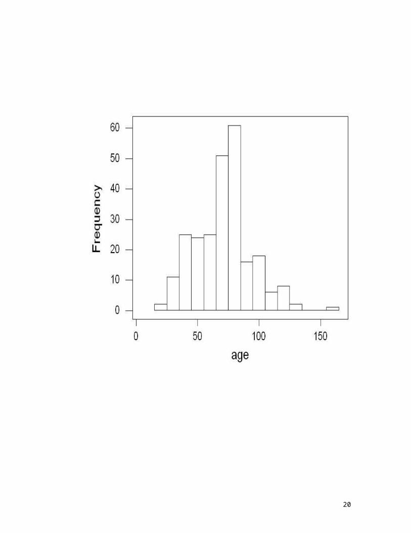
Example: 250 aspen trees of Alberta
15

Descriptive Statistics: age
N=250 trees Mean = 71 years
Median = 73 years
25% percentile = 55 75% percentile = 82
Minimum = 24 Maximum =160
Variance = 514.7 Standard Deviation = 22.69
1. Compare mean versus median2. Normal distribution?
Pearson correlation of age and dbh = 0.573 for the population of N=250 trees
16

Statistics from the Sample: 1. Mean -- e.g. for n=3 and y1=5;
y2=6; y3=7 , =6
2. Range: Maximum value – minimum value
3. Standard Deviation s and Variance s2
4. Standard Deviation of the sample means (also called the Standard Error, short for Standard Error of the Mean) and it’s square called the variance of the sample means are estimated by:
17

5. Coefficient of variation (CV): The standard deviation from the sample, divided by the sample mean. May be multiplied by 100 to get CV in percent.
6. Covariance between x and y: sxy
7. Correlation (Pearson’s) between two variables, y and x: r
Ranges from -1 to +1; with strong negative correlations near to -1 and strong positive correlations near to +1.
8. Distribution for y -- frequency of each value of y or x (may be divided into classes)
9. Estimated Probability Distribution of y or x – probability associated
18

with each y value based on the n observations
10.Mode -- most common value of y
or x
11. Median -- y-value or x-value which divides the estimated probability distribution (50% of N observations are above and 50% are below)
19
Example: n=150
20

n=150 trees Mean = 69 years
Median = 68 years
25% percentile = 48 75% percentile = 81
Minimum = 24 Maximum =160
Variance = 699.98 Standard Deviation = 25.69 years Standard error of the mean =2.12 years
Good estimate of population values?
Pearson correlation of age and dbh = 0.66 with a p-value of 0.000 for the sample of n=150 trees from a population of 250 trees
Null and alternative hypothesis for the p-value?What is a p-value?
21

Sample Statistics to Estimate Population Parameters:If simple random sampling (every observation has the same chance of being selected) is used to select n from N, then:
Sample estimates are unbiased estimates of their counterparts (e.g., sample mean estimates the population mean), meaning that over all possible samples the sample statistics, averaged, would equal the population statistic.
A particular sample value (e.g., sample mean) is called a “point estimate” -- do not necessarily equal the population parameter for a given sample.
Can calculate an interval where the true population parameter is likely to be, with a certain probability. This is a Confidence Interval, and can be obtained for any population
22

parameter, IF the distribution of the sample statistic is known.
Common continuous distributions:
Normal:
Symmetric distribution around μ Defined by μ and σ2. If we know
that a variable has a normal distribution, and we know these parameters, then we know the
23

probability of getting any particular value for the variable.
24

Probability tables are for μ=0 and σ2=1, and are often called z-tables.
Examples: P(-1<z<+1) = 0.68; P(-1.96<z<1.96)=0.95. Notation example: For α=0.05, .
z-scores: scale the values for y by subtracting the mean, and dividing by the standard deviation.
E.g., for mean=20, and standard deviation of 2 and y=10, z=-5.0 (an extreme value)
25

t-distribution: Symmetric distribution Table values have the center at 0.
The spread varies with the degrees of freedom. As the sample size increases, the df increases, and the spread decreases, and will approach the normal distribution.
Used for a normally distributed variable whenever the variance of that variable is not known.
Notation examples:where n-1 is the degrees of
freedom, in this case, and we are looking for the percentile. For example, for n=5 and α=0.05, we are looking for t with 4 degrees of freedom and the 0.975 percentile (will be a value around 2).
26

Χ2 distribution: Starts at zero, and is not
symmetric Is the square of a normally
distributed variable e.g. sample variances have a Χ2 distribution if the variable is normally distributed
Need the degrees of freedom and the percentile as with the t-distribution
27

28

F-distribution: Is the ratio of 2 variables that
each have a Χ2 distribution eg. The ratio of 2 sample variances for variables that are each normally distributed.
Need the percentile, and two degrees of freedom (one for the numerator and one for the denominator)
Central Limit Theorem: As n increases, the distribution of sample means will approach a normal distribution, even if the distribution is something else (e.g. could be non-symmetric)
Tables in the Textbook:Some tables give the values for probability distribution for the degrees of freedom, and for the percentile. Others, give this for the degrees of freedom and for the alpha level (or
29

sometimes alpha/2). Must be careful in reading probability tables.
Confidence Intervals for a single mean:
Collect data and get point estimates:
o The sample mean, to estimate of the
population mean ---- Will be unbiased
o The sample mean, to estimate of the
population mean ---- Will be unbiased
Can calculate interval estimates of each point
estimate e.g. 95% confidence interval for the
true mean
o If the y’s are normally distributed OR
o The sample size is large enough that the
Central Limit Theorem holds -- will be
normally distributed
30

31

32

Examples:
n is: 4
Plot volume ba/ha ave. dbh
1 200 34 502 150 20 403 300 40 554 0 0 0
mean: 162.50 23.50 36.25variance: 15625.00 315.67 622.92std.dev.: 125.00 17.77 24.96std.dev.of mean: 62.50 8.88 12.48t should be: 3.182Actual 95% CI(+/-): 198.88 28.27 39.71
NOTE:EXCEL: 95%(+/-)
122.50 17.41 24.46
t: 1.96 1.96 1.96not correct!!!
33

Hypothesis Tests: Can hypothesize what the true
value of any population parameter might be, and state this as null hypothesis (H0: )
We also state an alternate hypothesis (H1: or Ha: ) that it is a) not equal to this value; b) greater than this value; or c) less than this value
Collect sample data to test this hypothesis
From the sample data, we calculate a sample statistic as a point estimate of this population parameter and an estimated variance of the sample statistic.
We calculate a “test-statistic” using the sample estimates
Under H0, this test-statistic will follow a known distribution.
If the test-statistic is very unusual, compared to the tabular values for the known distribution, then the H0
34

is very unlikely and we conclude H1:
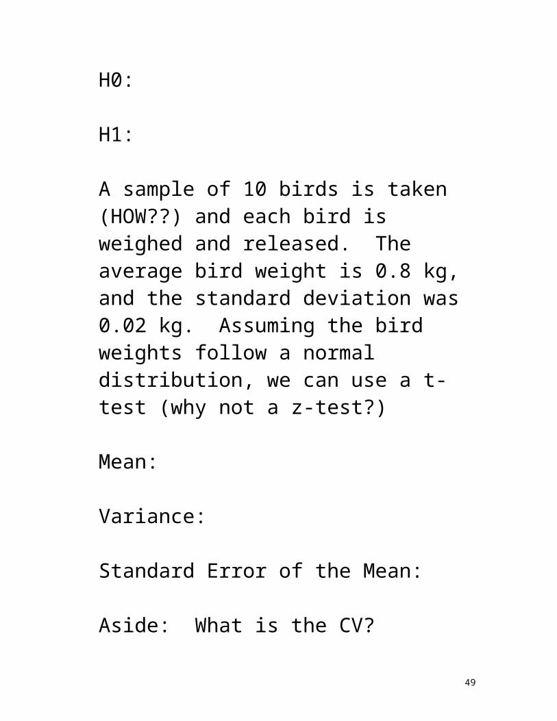
Example for a single mean:We believe that the average weight of ravens in Yukon is 1 kg.
H0:
H1:
A sample of 10 birds is taken (HOW??) and each bird is weighed and released. The average bird weight is 0.8 kg, and the standard deviation was 0.02 kg. Assuming the bird weights follow a normal distribution, we can use a t-test (why not a z-test?)
Mean:
35

Variance:
Standard Error of the Mean:
Aside: What is the CV?
Test statistic: t-distribution
t=
Under H0: this will follow a t-distribution with df = n-1.
Find value from t-table and compare:
Conclude?
36

The p-value:
Is the probability that we would get a value outside of the sample test statistic.
NOTE: In EXCEL use: =tdist(x,df,tails)
37

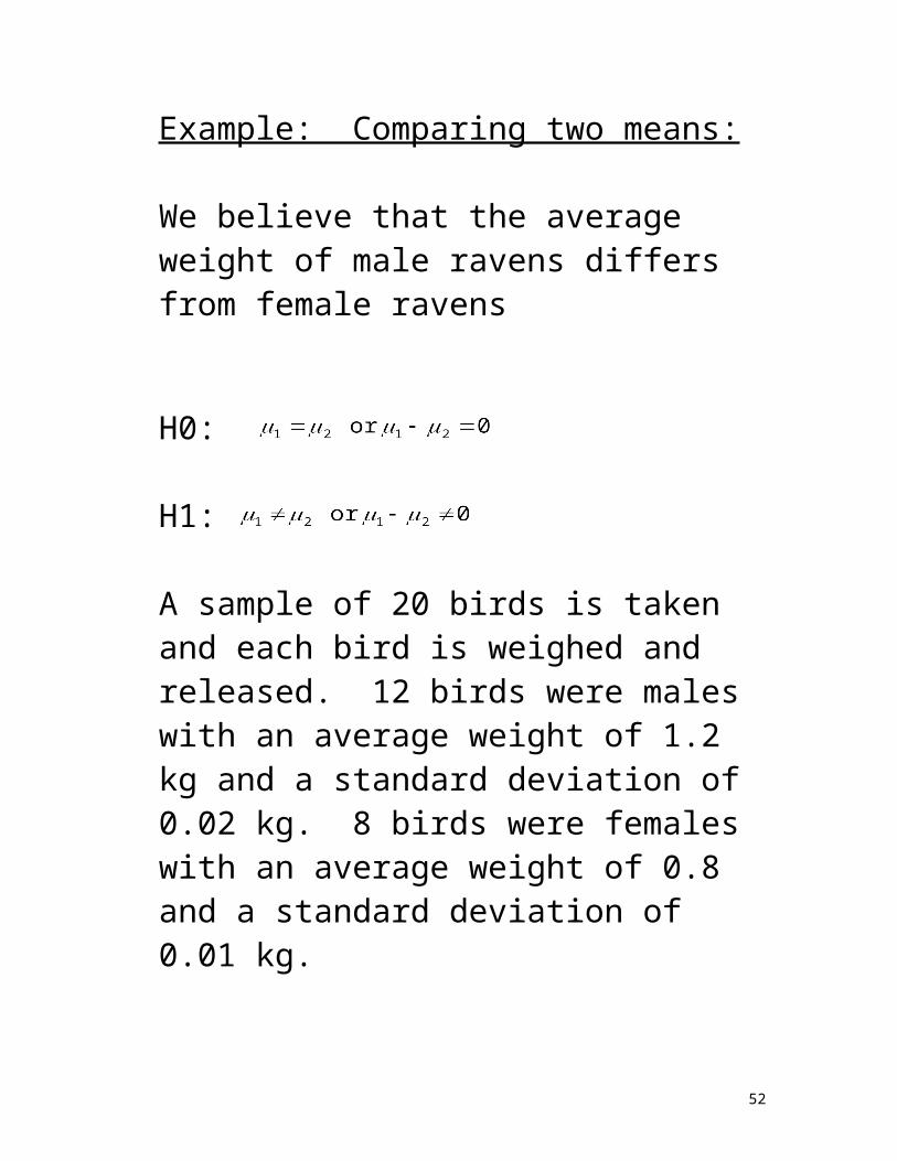
Example: Comparing two means:
We believe that the average weight of male ravens differs from female ravens
H0:
H1:
A sample of 20 birds is taken and each bird is weighed and released. 12 birds were males with an average weight of 1.2 kg and a standard deviation of 0.02 kg. 8 birds were females with an average weight of 0.8 and a standard deviation of 0.01 kg.
Means?
Sample Variances?
38

Test statistic:
t =
Under H0: this will follow a t-distribution with df = (n1+n2-2).
Find t-value from tables and compare, or use the p-value:
Conclude?
39

Errors for Hypothesis Tests
H0 True H0 FalseAccept 1-α β (Type II
error) Reject α (Type I
error)1-β
Type I Error: Reject H0 when it was true. Probability of this happening is α
Type II Error: Accept H0 when it is false. Probability of this happening is β
Power of the test: Reject H0 when it is false. Probability of this is 1-β
40

What increases power? Increase sample sizes, resulting in
lower standard errors
A larger difference between mean for H0 and for H1
Increase alpha. Will decrease beta.
Fitting Equations
41

REF:Idea is :- variable of interest (dependent variable) yi ; hard to measure- “easy to measure” variables (predictor/ independent) that are related to the variable of interest, labeled x1i , x2i,.....xmi
- measure yi, x1i,.....xmi for a sample of n items- use this sample to estimate an equation that relates yi (dependent variable) to x1i,..xmi (independent or predictor variables)- once equation is fitted, one can then just measure the x’s, and get an estimate of y without measuring it-- also can examine relationships between variables
42

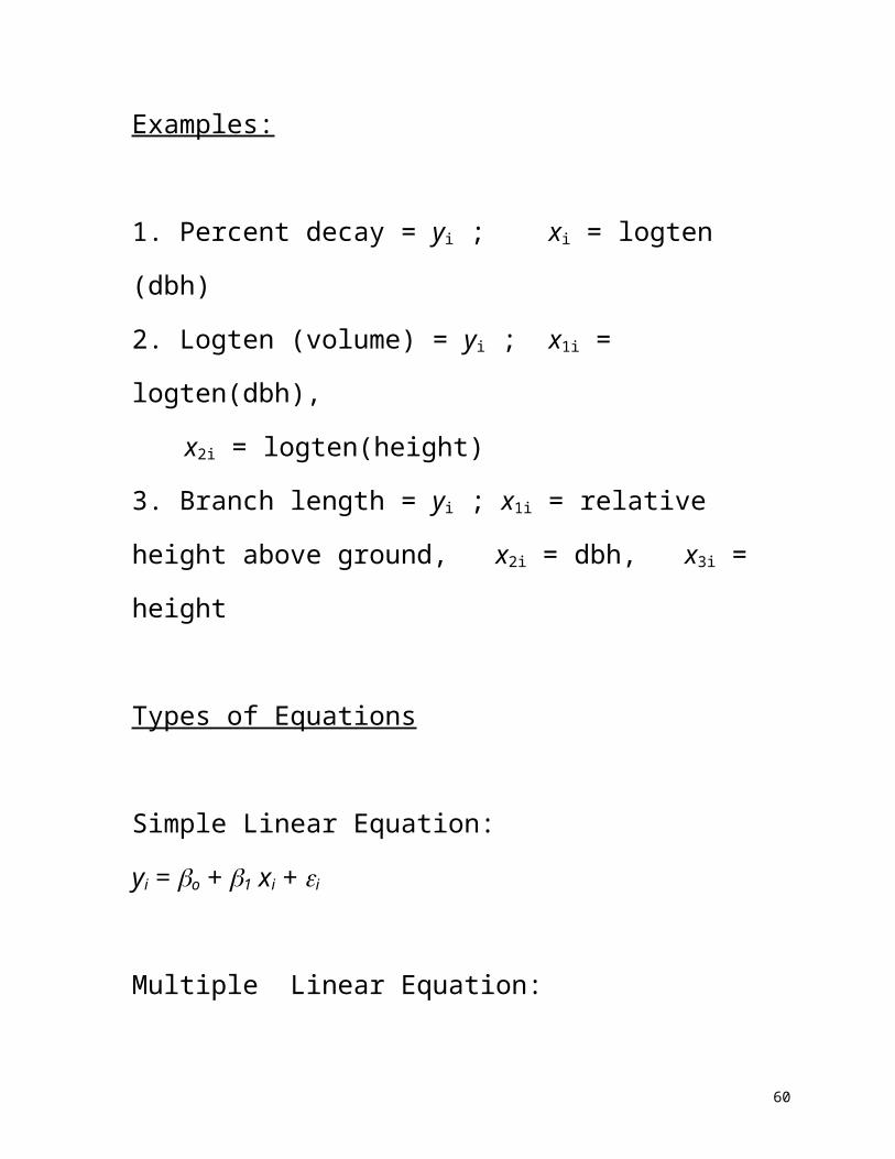
Examples:
1. Percent decay = yi ; xi = logten (dbh)2. Logten (volume) = yi ; x1i = logten(dbh),
x2i = logten(height)3. Branch length = yi ; x1i = relative height above ground, x2i = dbh, x3i = height
Types of Equations
Simple Linear Equation:yi = o + 1 xi + i
Multiple Linear Equation:yi = 0 + 1 x1i + 2 x2i +...+m xmi +i
Nonlinear Equation: takes many forms, for example:yi = 0 + 1 x1i 2 x 2i
3 +i
43

Objective:
Find estimates of 0, 1, 2 ... m such that the sum of squared differences between measured yi
and predicted yi (usually labeled as iy , values on the line or surface) is the smallest (minimize the sum of squared errors, called least squared error).
ORFind estimates of 0, 1, 2 ... m such that the likelihood (probability) of getting these y values is the largest (maximize the likelihood).
Finding the minimum of sum of squared errors is often easier. In some cases, they lead to the same estimates of parameters.
44

Simple Linear Regression (SLR)
Population: yi = 0 + 1 xi + i iY xx 10|
Sample: yi = b0 + b1 xi + ei iiiii yyexbby ˆˆ 10
b0 is an estimate of 0 [intercept]
b1 is an estimate of 1 [slope]
iy is the predicted y; an estimate of the average for y for a
particular x value
ei is an estimate of i, called the error or the residual;
represents the variation in the dependent variable (the y)
which is not accounted for by predictor variable (the x).
Find bo (intercept; yi when xi = 0) and b1 (slope) so that
SSE=ei2 (sum of squared errors over all n sample
observations) is the smallest (least squares solution)
The variables do not have to be in the same units.
Coefficients will change with different units of measure.
Given estimates of bo and b1, we can get an estimate of
the dependent variable (the y) for ANY value of the x,
within the ranges of x ’s represented in the original data.
45

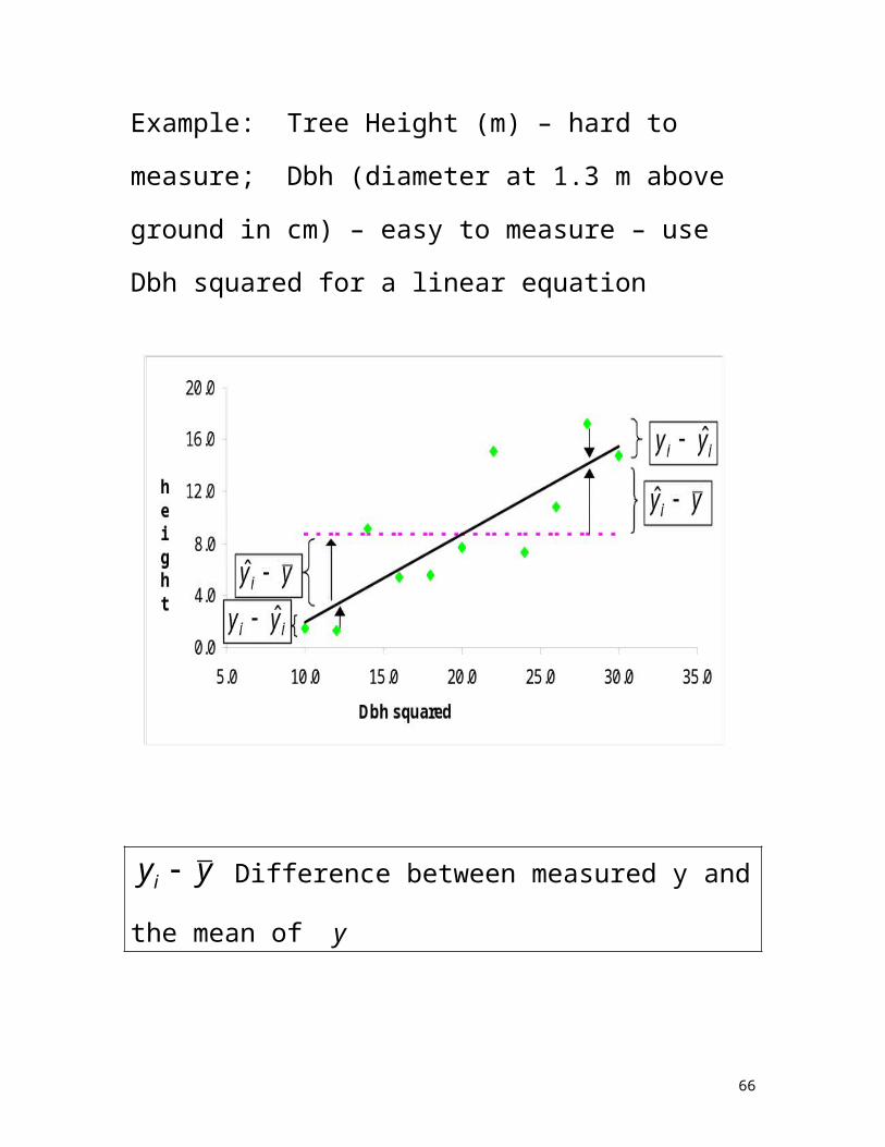
Example: Tree Height (m) – hard to measure; Dbh
(diameter at 1.3 m above ground in cm) – easy to measure
– use Dbh squared for a linear equation
yyi Difference between measured y and the mean of y
ii yy ˆ Difference between measured y and predicted y
iiii yyyyyy ˆˆ Difference between
predicted y and mean of y
46

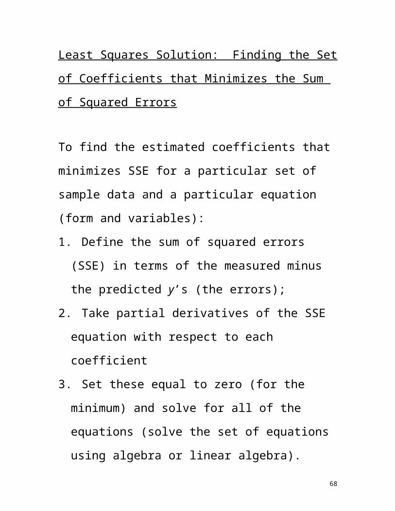
Least Squares Solution: Finding the Set of Coefficients
that Minimizes the Sum of Squared Errors
To find the estimated coefficients that minimizes SSE for a
particular set of sample data and a particular equation (form
and variables):
1. Define the sum of squared errors (SSE) in terms of the
measured minus the predicted y’s (the errors);
2. Take partial derivatives of the SSE equation with respect
to each coefficient
3. Set these equal to zero (for the minimum) and solve for
all of the equations (solve the set of equations using
algebra or linear algebra).
47

For linear models (simple or multiple linear), there will be one
solution. We can mathematically solve the set of partial
derivative equations.
WILL ALWAYS GO THROUGH THE POINT
DEFINED BY yx, .
Will always result in ei=0
For nonlinear models, this is not possible and we must search
to find a solution (covered in FRST 530).
If we used the criterion of finding the maximum likelihood
(probability) rather than the minimum SSE, we would need to
search for a solution, even for linear models (covered FRST
530).
48
Least Squares Solution for SLR:
Find the set of estimated parameters (coefficients) that minimize sum of squared errors
n
iii
n
ii xbbyeSSE
1
210
1
2 )(min)min()min(
Take partial derivatives with respect to b0 and b1, set them equal to zero and solve.
n
iii xbby
bSSE
110
0
)(2
n
ii
n
ii
n
ii
n
ii
n
ii
n
i
n
ii
xn
byn
b
xbnby
xbby
11
10
110
1
11
10
1
11
0
0
xbyb 10
49

n
iiii xbbyx
bSSE
110
1
)(2
n
ii
i
n
i
n
iii
n
ii
i
n
i
n
iii
i
n
i
n
iii
n
ii
n
iii
n
i
n
iii
x
xxbyxyb
x
xbxyb
xbxyxb
xbxbxy
1
2
11
11
1
2
10
11
10
11
21
1
21
10
1
)(
0
With some further manipulations:
SSxSPxy
nsns
xx
xxyyb
x
xy
n
ii
n
iii
)1()1(
2
2
1
2
11
Where SPxy refers to the corrected sum of cross products for x and y; SSx refers to the corrected sum of squares for x [Class example]
50

Properties of b0 and b1
b0 and b1 are least squares estimates of 0 and 1 . Under assumptions concerning the error term and sampling/ measurements, these are: Unbiased estimates; given many estimates of the slope
and intercept for all possible samples, the average of the sample estimates will equal the true values
The variability of these estimates from sample to sample can be estimated from the single sample; these estimated variances will be unbiased estimates of the true variances (and standard errors)
The estimated intercept and slope will be the most precise (most efficient with the lowest variances) estimates possible (called “Best”)
These will also be the maximum likelihood estimates of the intercept and slope
51
Assumptions of SLR
Once coefficients are obtained, we must check the
assumptions of SLR. Assumptions must be met to:
obtain the desired characteristics
assess goodness of fit (i.e., how well the regression
line fits the sample data)
test significance of the regression and other
hypotheses
calculate confidence intervals and test hypothesis for
the true coefficients (population)
calculate confidence intervals for mean predicted y
value given a set of x value (i.e. for the predicted y
given a particular value of the x)
Need good estimates (unbiased or at least consistent) of
the standard errors of coefficients and a known
probability distribution to test hypotheses and calculate
confidence intervals.
52

Checking assumptions using residual Plots
Assumptions of :
1. a linear relationship between the y and the x;
2. equal variance of errors; and
3. independence of errors (independent observations)
can be visually checked by using RESIDUAL PLOTS
A residual plot shows the residual (i.e., yi - iy ) as the y-axis
and the predicted value ( iy ) as the x-axis.
Residual plots can also indicate unusual points (outliers)
that may be measurement errors, transcription errors, etc.
53

Residual plot that meets the assumptions of a linear
relationship, and equal variance of the observations:
The data points are evenly distributed about zero and there
are no outliers (very unusual points that may be a
measurement or entry error).
For independence:
54

Examples of Residual Plots Indicating Failures to Meet
Assumptions:
1. The relationship between the x’s and y is linear. If not met,
the residual plot and the plot of y vs. x will show a curved line:
ht ‚60 ˆ ‚ ‚ ‚ ‚ 1 ‚ 2 150 ˆ 1 1 11 1 ‚ 1 2 1121 1 1 1 2 ‚ 2 2 21 1 1 1 1 ‚ 2 2 122 1 1 21 1 2 1 111 ‚ 2 2 22 22222 2 2 1 ‚ 2 12 121 140 ˆ 2 22 12 11221 1 ‚ 2 222 2 22 22 1 ‚ 22 2 22 1 22 1 ‚ 22 2 2 22 1 1 ‚ 2 2222122 11 ‚ 22 221222 2 230 ˆ 3 2232222 ‚ 22323 2 2 ‚ 232231123 1 2 ‚ 322333212 2 ‚ 333324311 13 ‚ 4133311 1 320 ˆ 22213113 3 3 ‚ 233313 3 ‚ 43313 ‚ 43 ‚ 443 ‚ 33210 ˆ 42 ‚ ‚ ‚ ‚ ‚ 0 ˆ ‚ Šˆ------------ˆ------------ˆ------------ˆ------------ˆ------------ˆ 0 2000 4000 6000 8000 10000
dbhsq
Residual ‚ ‚ 15 ˆ ‚ * ‚ * * ‚ * ‚ * * 10 ˆ * * ‚ *** * *** ‚ *** *** ** ‚ ** * *** ***** ‚ *** *** * *** * 5 ˆ ********* ** ******* * ‚ **** * ** ** * ‚ ****** *** ** * ‚ ***** ** * ** *** * * * ‚ ***** ** * * * **** 0 ˆ ******** ** *** ‚ ******** * * * * ** ‚ ******* * * ‚ ******* ** * * * ‚ ******* * * * -5 ˆ * *** * * * * * ‚ * ** ‚ ** * * ** * ‚ ** * * * ‚ ** ** -10 ˆ * * ‚ * * ‚ * * * ‚ ‚ -15 ˆ * ‚ * ‚ ‚ ‚ -20 ˆ ‚ Š-ˆ---------ˆ---------ˆ---------ˆ---------ˆ---------ˆ---------ˆ- 10 20 30 40 50 60 70
Predicted Value of ht
Result: If this assumption is not met: the regression line
does not fit the data well; biased estimates of coefficients
and standard errors of the coefficients will occur
55

2. The variance of the y values must be the same for
every one of the x values. If not met, the spread around the
line will not be even.
Result: If this assumption is not met, the estimated
coefficients (slopes and intercept) will be unbiased, but the
estimates of the standard deviation of these coefficients will
be biased.
we cannot calculate CI nor test the significance of the x
variable. However, estimates of the coefficients of the
regression line and goodness of fit are still unbiased
56

3. Each observation (i.e., xi and yi) must be independent of
all other observations. In this case, we produce a different
residual plot, where the residuals are on the y-axis as
before, but the x-axis is the variable that is thought to
produce the dependencies (e.g., time). If not met, this
revised residual plot will show a trend, indicating the
residuals are not independent.
Result: If this assumption is not met, the estimated
coefficients (slopes and intercept) will be unbiased, but the
estimates of the standard deviation of these coefficients will
be biased.
57

we cannot calculate CI nor test the significance of the x
variable. However, estimates of the coefficients of the
regression line and goodness of fit are still unbiased
Normality Histogram or Plot
A fourth assumption of the SLR is:
4. The y values must be normally distributed for each of
the x values. A histogram of the errors, and/or a normality
plot can be used to check this, as well as tests of normality Histogram # Boxplot 10.5+* 1 0 .* 1 | .* 2 | .* 2 | .**** 8 | .******* 14 | .************** 27 | .******************** 40 | .***************************** 57 +-----+ .************************** 51 | | .****************************** 60 *--+--* -0.5+***************************** 58 | | .************************* 49 | | .***************** 33 +-----+ .************** 28 | .************ 24 | .*********** 22 | .**** 7 | .**** 7 | .*** 5 | . .* 1 0 -11.5+** 3 0 ----+----+----+----+----+----+
HO: data are normal H1: data are not normalTests for Normality
Test --Statistic--- -----p Value------Shapiro-Wilk W 0.991021 Pr < W 0.0039Kolmogorov-Smirnov D 0.039181 Pr > D 0.0617Cramer-von Mises W-Sq 0.19362 Pr > W-Sq 0.0066
58

Anderson-Darling A-Sq 1.193086 Pr > A-Sq <0.0050
Normal Probability Plot 10.5+ * | * | +** | +++** | +**** | +**** | ***** | **** | ***** | **** | **** -0.5+ **** | ***+ | **** | *** | +*** | ***** | +** | +*** |+**** | | * -11.5+* +----+----+----+----+----+----+----+----+----+----+
Result: We cannot calculate CI nor test the significance of
the x variable, since we do not know what probabilities to
use. Also, estimated coefficients are no longer equal to the
maximum likelihood solution.
Example:
59
60
3210-1-2-3
43
21
0-1
-2
Normal Plot of Residuals
Normal Score
Resid
ual
43210-1-2
100
50
0
Residual
Fre
quency
Histogram of Residuals
250200150100500
43210
-1-2-3
Observation NumberR
esid
ual
I Chart of Residuals
566
6
6
52
2222
2
2
22222
22
22
2
2
2
22222
2
22
66
22222
222
222
7
7
62
11
11
777
11
6
1
1
5
22
X=0.000
UCL=2.263
LCL=-2.263
1050
4
3
2
1
0
-1
-2
Fit
Resid
ual
Residuals vs. Fits
Volume versus dbh

Measurements and Sampling Assumptions
The remaining assumptions are based on the measurements
and collection of the sampling data.
5. The x values are measured without error (i.e., the x
values are fixed).
This can only be known if the process of collecting the data
is known. For example, if tree diameters are very precisely
measured, there will be little error. If this assumption is not
met, the estimated coefficients (slopes and intercept) and
their variances will be biased, since the x values are
varying.
61

6. The y values are randomly selected for value of the x
variables (i.e., for each x value, a list of all possible y
values is made, and some are randomly selected).
For many biological problems, the observations will be
gathered using simple random sampling or systematic
sampling (grid across the land area). This does not strictly
meet this assumption. Also, more complex sampling
design such as multistage sampling (sampling large units
and sampling smaller units within the large units), this
assumption is not met. If the equation is “correct”, then
this does not cause problems. If not, the estimated equation
will be biased.
62

Transformations
Common Transformations
Powers x3, x0.5, etc. for relationships that look
nonlinear
log10, loge also for relationships that look nonlinear,
or when the variances of y are not equal around the
line
Sin-1 [arcsine] when the dependent variable is a
proportion.
Rank transformation: for non-normal data
o Sort the y variable
o Assign a rank to each variable from 1 to n
o Transform the rank to normal (e.g., Blom
Transformation)
PROBLEM: loose some of the information in the
original data
Try to transform x first and leave yi = variable of
interest; however, this is not always possible.
Use graphs to help choose transformations
63

Outliers: Unusual Points
Check for points that are quite different from the others on:
Graph of y versus x
Residual plot
Do not delete the point as it MAY BE VALID! Check:
Is this a measurement error? E.g., a tree height of 100
m is very unlikely
Is a transcription error? E.g. for adult person, a weight
of 20 lbs was entered rather than 200 lbs.
Is there something very unusual about this point? e.g.,
a bird has a short beak, because it was damaged.
Try to fix the observation. If it is very different than the
others, or you know there is a measurement error that
cannot be fixed, then delete it and indicate this in your
research report.
On the residual plot, an outlier CAN occur if the model is
not correct – may need a transformation of the variable(s),
or an important variable is missing
64

Other methods, than SLR (and Multiple Linear Regression), when
transformations do not work (some covered in FRST 530):
Nonlinear least squares: Least squares solution for nonlinear
models; uses a search algorithm to find estimated coefficients; has
good properties for large datasets; still assumes normality, equal
variances, and independent observations
Weighted least squares: for unequal variances. Estimate the
variances and use these in weighting the least squares fit of the
regression; assumes normality and independent observations
General linear model: used for distributions other than normal
(e.g., binomial, Poisson, etc.), but with no correlation between
observations; uses maximum likelihood
Generalized least Squares and Mixed Models: use maximum
likelihood for fitting models with unequal variances, correlations
over space, correlations over time, but normally distributed errors
General linear mixed models: Allows for unequal variances,
correlations over space and/or time, and non-normal distributions;
uses maximum likelihood
65
Measures of Goodness of Fit
How well does the regression fit the sample data?
For simple linear regression, a graph of the original
data with the fitted line marked on the graph indicates
how well the line fits the data [not possible with MLR]
Two measures commonly used: coefficient of
determination (r2) and standard error of the
estimate(SEE).
66

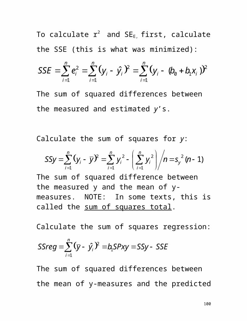
To calculate r2 and SEE, first, calculate the SSE (this is what
was minimized):
n
iii
n
iii
n
ii xbbyyyeSSE
1
210
1
2
1
2 )(ˆ
The sum of squared differences between the measured and
estimated y’s.
Calculate the sum of squares for y:
)1(2
1
2
1
2
1
2
nsnyyyySSy y
n
ii
n
ii
n
ii
The sum of squared difference between the measured y and the mean of y-measures. NOTE: In some texts, this is called the sum of squares total.
Calculate the sum of squares regression:
SSESSySPxybyySSregn
ii
1
1
2ˆ
The sum of squared differences between the mean of y-
measures and the predicted y’s from the fitted equation.
Also, is the sum of squares for y – the sum of squared
errors.
67
Then: SSySSreg
SSySSE
SSySSESSyr
12
SSE, SSY are based on y’s used in the equation –
will not be in original units if y was transformed
r2 = coefficient of determination; proportion of
variance of y, accounted for by the regression using x
Is the square of the correlation between x and y
O (very poor – horizontal surface representing no
relationship between y and x’s) to 1 (perfect fit –
surface passes through the data)
And:2
nSSESEE
SSE is based on y’s used in the equation – will not
be in original units if y was transformed
SEE - standard error of the estimate; in same units as
y
Under normality of the errors:
o 1 SEE 68% of sample observations
o 2 SEE 95% of sample observations
o Want low SEE
68

y-variable was transformed: Can calculate estimates of
these for the original y-variable unit, called I2 (Fit Index)
and estimated standard error of the estimate (SEE’), in order
to compare to r2 and SEE of other equations where the y was
not transformed.
I2 = 1 - SSE/SSY
where SSE, SSY are in original units. NOTE must
“back-transform” the predicted y’s to calculate the
SSE in original units.
Does not have the same properties as r2, however:
o it can be less than 0
o it is not the square of the correlation between the
y (in original units) and the x used in the
equation.
Estimated standard error of the estimate (SEE’) , when the
dependent variable, y, has been transformed:
2)('
nunitsoriginalSSESEE
SEE’ - standard error of the estimate ; in same units
as original units for the dependent variable
want low SEE’ [Class example]
69

Estimated Variances, Confidence Intervals and Hypothesis
Tests
Testing Whether the Regression is Significant
Does knowledge of x improve the estimate of the mean of y?
Or is it a flat surface, which means we should just use the
mean of y as an estimate of mean y for any x?
SSE/ (n-2):
Called the Mean squared error, as would be the average
of the squared error if we divided by n.
Instead, we divide by n-2. Why? The degrees of freedom
are n-2; n observations with two statistics estimated from
these, b0 and b1
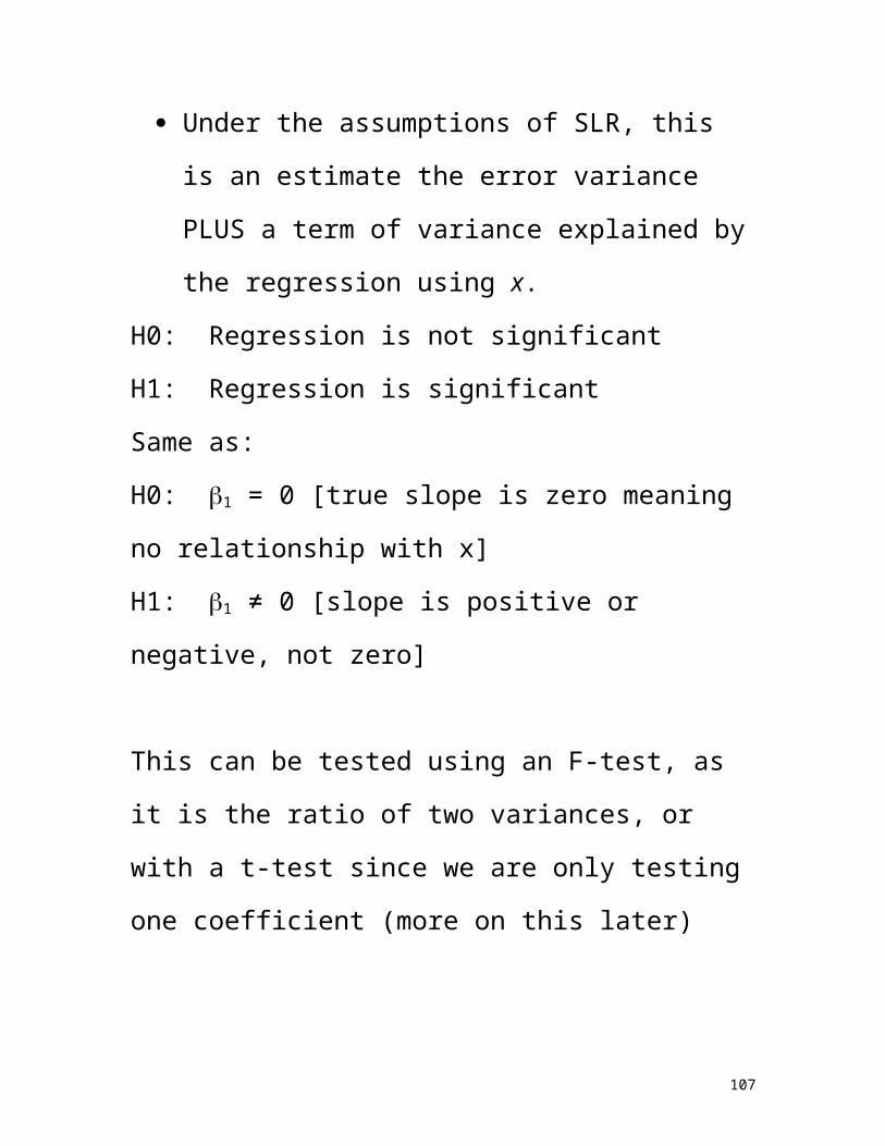
Under the assumptions of SLR, is an unbiased estimated
of the true variance of the error terms (error variance)
SSR/1:
Called the Mean Square Regression
Degrees of Freedom=1: 1 x-variable
Under the assumptions of SLR, this is an estimate the
error variance PLUS a term of variance explained by
the regression using x.
H0: Regression is not significant
70

H1: Regression is significant
Same as:
H0: 1 = 0 [true slope is zero meaning no relationship with
x]
H1: 1 ≠ 0 [slope is positive or negative, not zero]
This can be tested using an F-test, as it is the ratio of two
variances, or with a t-test since we are only testing one
coefficient (more on this later)
Using an F test statistic:
MSEMSreg
nSSESSreg
F
)2(
1
Under H0, this follows an F distribution for a 1- α/2
percentile with 1 and n-2 degrees of freedom.
If the F for the fitted equation is larger than the F from
the table, we reject H0 (not likely true). The
regression is significant, in that the true slope is likely
not equal to zero.
71

Information for the F-test is often shown as an Analysis of Variance Table:
Source df SS MS F p-valueRegression 1
SSregMSreg=SSreg/1
F= MSreg/MSE
Prob F> F(1,n-2,1- α)
Residual n-2 SSE MSE= SSE/(n-2)
Total n-1 SSy
[Class example and explanation of the p-value]
72

Estimated Standard Errors for the Slope and Intercept
Under the assumptions, we can obtain an unbiased
estimated of the standard errors for the slope and for the
intercept [measure of how these would vary among
different sample sets], using the one set of sample data.
SSxMSEs
SSxn
xMSE
SSxx
nMSEs
b
n
ii
b
1
0
1
221
Confidence Intervals for the True Slope and Intercept
Under the assumptions, confidence intervals can be
calculated as:
For o: 02,210 bn stb
For 1: 12,211 bn stb
[class example]
73

Hypothesis Tests for the True Slope and Intercept
H0: 1 = c [true slope is equal to the constant, c]
H1: 1 ≠ c [true slope differs from the constant c]
Test statistic:
1
1
bscb
t
Under H0, this is distributed as a t value of tc = tn-2, 1-/2.
Reject Ho if t > tc.
The procedure is similar for testing the true intercept
for a particular value
It is possible to do one-sided hypotheses also, where
the alternative is that the true parameter (slope or
intercept) is greater than (or less than) a specified
constant c. MUST be careful with the tc as this is
different.
[class example]
74

Confidence Interval for the True Mean of y given a
particular x value
For the mean of all possible y-values given a particular
value of x (y|xh):
hxynh stxy |ˆ21,2|ˆ
where
SSxxx
nMSEs
xbbxy
hxy
hh
h
2
|ˆ
10
1
|ˆ
75

Confidence Bands
Plot of the confidence intervals for the mean of y for
several x-values. Will appear as:
0.02.0
4.06.0
8.010.012.0
14.016.0
18.020.0
5.0 10.0 15.0 20.0 25.0 30.0 35.0
76

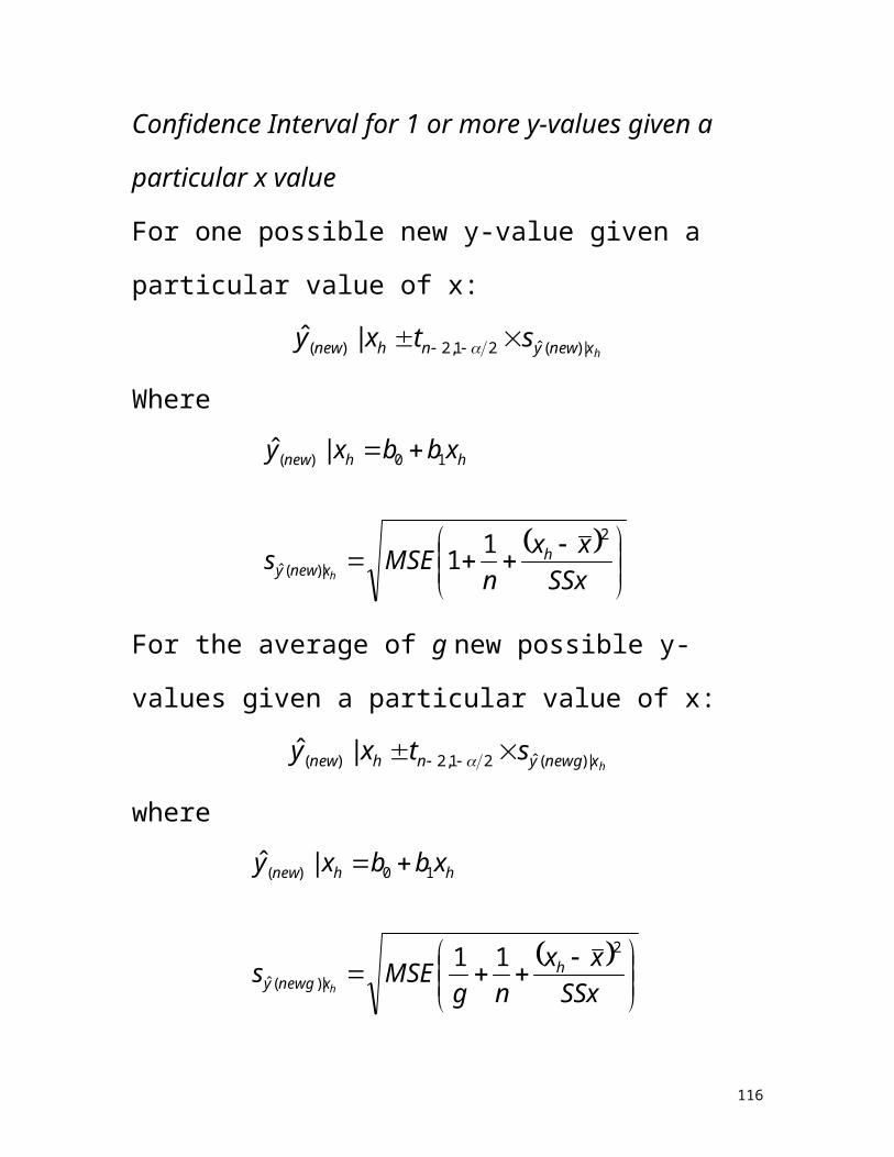
Confidence Interval for 1 or more y-values given a
particular x value
For one possible new y-value given a particular value of x:
hxnewynhnew stxy |)(ˆ21,2)( |ˆ
Where
SSxxx
nMSEs
xbbxy
hxnewy
hhnew
h
2
|)(ˆ
10)(
11
|ˆ
For the average of g new possible y-values given a
particular value of x:
hxnewgynhnew stxy |)(ˆ21,2)( |ˆ
where
SSxxx
ngMSEs
xbbxy
hxgnewy
hhnew
h
2
|)(ˆ
10)(
11
|ˆ
[class example]
77
Selecting Among Alternative Models
Process to Fit an Equation using Least Squares
Steps:
1. Sample data are needed, on which the dependent variable
and all explanatory (independent) variables are
measured.
2. Make any transformations that are needed to meet the
most critical assumption: The relationship between y
and x is linear.
Example: volume = 0 + 1 dbh2 may be linear whereas
volume versus dbh is not. Use yi = volume , xi = dbh2.
3. Fit the equation to minimize the sum of squared error.
4. Check Assumptions. If not met, go back to Step 2.
5. If assumptions are met, then interpret the results.
Is the regression significant?
What is the r2? What is the SEE?
Plot the fitted equation over the plot of y versus x.
78

For a number of models, select based on:
1. Meeting assumptions: If an equation does not meet the
assumption of a linear relationship, it is not a candidate
model
2. Compare the fit statistics. Select higher r2 (or I2), and
lower SEE (or SEE’)
3. Reject any models where the regression is not
significant, since this model is no better than just using
the mean of y as the predicted value.
4. Select a model that is biologically tractable. A simpler
model is generally preferred, unless there are
practical/biological reasons to select the more complex
model
5. Consider the cost of using the model
[class example]
79

Simple Linear Regression Example
Temperature (x)
Weight (y)
Weight(y)
Weight(y)
0 8 6 815 12 10 1430 25 21 2445 31 33 2860 44 39 4275 48 51 44
Observation temp weight1 0 82 0 63 0 84 15 125 15 106 15 147 30 258 30 21
Et cetera…
80

weight versus temperature
0
10
20
30
40
50
60
0 10 20 30 40 50 60 70 80
temperature
wei
ght
81

Obs. tempweigh
t x-diff x-diff. sq.
1 0 8-
37.50 1406.25
2 0 6-
37.50 1406.25
3 0 8-
37.50 1406.25
4 15 12-
22.50 506.25Et
cetera
mean 37.5 27.11
SSX=11,812.5 SSY=3,911.8 SPXY=6,705.0
xbybSSx
SPxyb 101
b1: 0.567619
82

b0: 5.825397
NOTE: calculate b1 first, since this is needed to calculate b0.
83

From these, the residuals (errors) for the equation, and the sum of squared error (SSE) were calculated:
Obs. weight y-pred residualresidual
sq.1 8 5.83 2.17 4.732 6 5.83 0.17 0.033 8 5.83 2.17 4.734 12 14.34 -2.34 5.47
Et cetera
SSE: 105.89
And SSR=SSY-SSE=3805.89
ANOVA
Source df SS MSModel 1 3805.89 3805.89
Error 18-2=16 105.89 6.62
Total18-1=17 3911.78
84

F=575.06 with p=0.00 (very small)
In excel use: = fdist(x,df1,df2) to obtain a “p-value”
r2: 0.97Root MSE Or SEE : 2.57
BUT: Before interpreting the ANOVA table, Are assumptions met?
85

residual plot
-6.00
-4.00
-2.00
0.00
2.00
4.00
6.00
0.00 10.00 20.00 30.00 40.00 50.00 60.00
predicted weight
residu
als (error
s)
Linear?
Equal variance?
Independent observations?
86

Normality plot:
Obs. sorted Stand. Rel. Prob.
resids resids Freq.z-
dist.1 -4.40 -1.71 0.06 0.042 -4.34 -1.69 0.11 0.053 -3.37 -1.31 0.17 0.104 -2.34 -0.91 0.22 0.185 -1.85 -0.72 0.28 0.246 -0.88 -0.34 0.33 0.377 -0.40 -0.15 0.39 0.448 -0.37 -0.14 0.44 0.449 -0.34 -0.13 0.50 0.45
Etc.
87

Probability plot
0.00
0.20
0.40
0.60
0.80
1.00
1.20
-2.00 -1.00 0.00 1.00 2.00
z-value
cum
ulat
ive
prob
abili
ty
relative frequency
Prob. z-dist.
88

Questions:
1. Are the assumptions of simple linear regression met? Evidence?
2. If so, interpret if this is a good equation based on goodness of it measures.
89
3. Is the regression significant?
90

For 95% confidence intervals for b0 and b1, would also need estimated standard errors:
0237.050.11812
62.6
075.150.11812
5.3718162.61
1
0
22
SSxMSEs
SSxx
nMSEs
b
b
The t-value for 16 degrees of freedom and the 0.975 percentile is 2.12 (=tinv(0.05,16) in EXCEL)
91

For o: 075.1120.2825.5
02,210
bn stb
For 1: 0237.0120.2568.0
12,211
bn stb
Est. Coeff St. Error
For b0:5.82539682
5 1.074973559
For b1:0.56761904
8 0.023670139
CI: b0 b1t(0.975,16) 2.12 2.12
lower 3.546452880.51743835
3
upper8.10434077
10.61779974
2
92

Question: Could the real intercept be equal
to 0?
Given a temperature of 22, what is the
estimated average weight (predicted value)
and a 95% confidence interval for this
estimate?
709.0
50.118125.3722
18162.6
1
313.1822568.0825.5)22(|ˆ|ˆ
2
|ˆ
2
|ˆ
10
h
h
xy
hxy
h
hh
s
SSxxx
nMSEs
xyxbbxy
93

816.19709.012.2313.18810.16709.012.2313.18
|ˆ |ˆ21,2
hxynh stxy
94

Given a temperature of 22, what is the
estimated weight for any new observation,
and a 95% confidence interval for this
estimate?
669.2
50.118125.3722
181162.6
11
313.1822568.0825.5)22(|ˆ|ˆ
2
|ˆ
2
|ˆ
10
h
h
xy
hxy
h
hh
s
SSxxx
nMSEs
xyxbbxy
97.23669.212.2313.1866.12669.212.2313.18
|ˆ |ˆ21,2
hxynh stxy
95
If assumptions were not met, we would
have to make some transformations and
start over again!
96

SAS code:* wttemp.sas-------------------------------------;options ls=70 ps=50; run;DATA regdata; input temp weight; cards; 0 8 0 6 0 8 15 12 15 10 15 14 30 25 30 21 30 24 45 31 45 33 45 28 60 44 60 39 60 42 75 48 75 51 75 44 run;
97

DATA regdata2;set regdata; tempsq=temp**2; tempcub=temp**3; logtemp=log(temp);run;Proc plot data=regdata2;plot weight*(temp tempsq logtemp)='*';run;*-------------------------------------------;PROC REG data=regdata2 simple; model weight=temp; output out=out1 p=yhat1 r=resid1;run;*----------------------------------------------;PROC PLOT DATA=out1; plot resid1*yhat1;run;*-------------------------------------------;PROC univariate data=out1 plot normal;Var resid1;Run;
98

SAS outputs:
1) Graphs – which appears more linear?2) How many observations were there?3) What is the mean weight?
The REG Procedure Model: MODEL1 Dependent Variable: weight
Number of Observations Read 18 Number of Observations Used 18
Analysis of Variance
Sum of Mean Source DF Squares Square F Value Model 1 3805.88571 3805.88571 575.06 Error 16 105.89206 6.61825 Corr. Total 17 3911.77778
Source F Value Pr > F Model 575.06 <.0001 Error Corrected Total
Root MSE 2.57260 R-Square 0.9729 Dependent Mean 27.11111 Adj R-Sq 0.9712 Coeff Var 9.48909
99
Parameter Estimates Parameter StandardVariable DF Estimate Error t Value Intercept 1 5.82540 1.07497 5.42 temp 1 0.56762 0.02367 23.98
Variable t Value Pr > |t| Intercept 5.42 <.0001 temp 23.98 <.0001
100

Plot of resid1*yhat1. Legend: A = 1 obs, B = 2 obs, etc.
‚ 6 ˆ ‚ ‚ ‚ ‚ ‚ 4 ˆ A ‚ ‚ ‚ ‚ A ‚ B 2 ˆ A A ‚ AR ‚e ‚ As ‚i ‚ Ad 0 ˆu ‚ A A Aa ‚l ‚ A ‚ ‚ -2 ˆ A ‚ A ‚ ‚ ‚ A ‚ -4 ˆ ‚ A A ‚ ‚ ‚ ‚ -6 ˆ ---------------------------------------------------- 5.825 14.340 22.854 31.368 39.883 48.397
Predicted Value of weight
101

Tests for Normality
Test --Statistic--- --p Value---Shapiro-Wilk W 0.94352 Pr<W 0.3325Kolmogorov-Smirnov D 0.13523 Pr>D >0.1500Cramer-von Mises W-Sq 0.061918 Pr>W-Sq >0.2500Anderson-Darling A-Sq 0.407571 Pr>A-Sq >0.2500
The UNIVARIATE Procedure Variable: resid1 (Residual)
Normal Probability Plot
4.5+ +*++ | ++++ | * **++++* 1.5+ * *++++ | +*+++ | **+** -1.5+ +*++ | ++++* | ++++ * -4.5+ ++*+ * +----+----+----+----+----+----+----+----+----+----+ -2 -1 0 +1 +2
102

Multiple Linear Regression (MLR)
Population: yi = 0 + 1 x 1i + 2 x 2i +...+p xmi+i
Sample: yi = b0 + b1 x 1i + b2 x 2i +...+bp xmi +ei
iiimimiii yyexbxbxbby ˆˆ 22110
o is the y intercept parameter
1, 2, 3, ..., m are slope parameters
x1i, x2i, x3i ... xmi independent variables
i - is the error term or residual
- is the variation in the dependent variable (the y)
which is not accounted for by the independent variables
(the x’s).
For any fitted equation (we have the estimated parameters),
we can get the estimated average for the dependent
variable, for any set of x’s. This will be the “predicted”
value for y, which is the estimated average of y, given the
particular values for the x variables. NOTE: In text by
Neter et al. p=m+1. This is not be confused with the p-
value indicating significance in hypothesis tests.
103

For example:
Predicted log10(vol) = - 4.2 + 2.1 X log10(dbh) + 1.1 X log10(height)
where bo= -4.2; b1= 2.1 ; b1= 1.1 estimated by finding the
least squared error solution.
Using this equation for dbh =30 cm, height=28m,
logten(dbh) =1.48, logten(height) =1.45; logten(vol) =
0.503. volume (m3) = 3.184. This represents the
estimated average volume for trees with dbh=30 cm and
height=28 m.
Note: This equation is originally a nonlinear equation:
cb htdbhavol
Which was transformed to a linear equation using
logarithms:
10log)(10log)(10log)(10log)(10log htcdbhbavol
And this was fitted using multiple linear regression
104

For the observations in the sample data used to fit the
regression, we can also get an estimate of the error (we
have measured volume).
If the measured volume for this tree was 3.000 m3, or 0.477
in log10 units:
026.0503.0477.0ˆ ii yyerror
For the fitted equation using log10 units. In original units,
the estimated error is 3.000-3.184= - 0.184
NOTE: This is not simply the antilog of -0.026.
105

Finding the Set of Coefficients that Minimizes the Sum of
Squared Errors
Same process as for SLR: Find the set of coefficients that
results in the minimum SSE, just that there are more
parameters, therefore more partial derivative equations
and more equations
o E.g., with 3 x-variables, there will be 4 coefficients
(intercept plus 3 slopes) so four equations
For linear models, there will be one unique mathematical
solution.
For nonlinear models, this is not possible and we must
search to find a solution
Using the criterion of finding the maximum likelihood
(probability) rather than the minimum SSE, we would need to
search for a solution, even for linear models (covered in other
courses, e.g., FRST 530).
106
Least Squares Method for MLR:
Find the set of estimated parameters (coefficients) that minimize sum of squared errors
n
iimpiii
n
ii
xbxbxbby
eSSE
1
222110
1
2
)...(min
)min()min(
Take partial derivatives with respect to each of the variables, set them equal to zero and solve.
For three x-variables we obtain:
3322110 xbxbxbyb
1
313
1
212
1
11 SSx
xSPxbSSx
xSPxbSSx
ySPxb
2
323
2
211
2
22 SSx
xSPxbSSx
xSPxbSSx
ySPxb
3
322
3
311
3
33 SSx
xSPxbSSx
xSPxbSSx
ySPxb
107

Where SP= indicates sum of products between two variables, for example for y with x1:
)1(1211
1
11
1111
nsn
yxxy
xxyyySPx
yx
n
ii
n
iin
iii
n
iii
And SS indicates sums of squares for one variable, for example for x1:
)1(12
2
11
1
21
1
2111
nsn
xxxxSSx x
n
iin
ii
n
ii
108

Properties of a least squares regression “surface”:
1. Always passes through ),,...,,,( 321 yxxxx m
2. Sum of residuals is zero, i.e., ei=0
3. SSE the least possible (least squares)
4. The slope for a particular x-variable is AFFECTED
by correlation with other x-variables: CANNOT
interpret the slope for a particular x-variable,
UNLESS it has zero correlation with all other x-
variables (or nearly zero if correlation is estimated
from a sample).
[class example]
109

M eeting Assumptions of MLR
Once coefficients are obtained, we must check the
assumptions of MLR before we can:
assess goodness of fit (i.e., how well the regression
line fits the sample data)
test significance of the regression
calculate confidence intervals and test hypothesis
For these test to be valid, assumptions of MLR
concerning the observations and the errors (residuals)
must be met.
110

Residual Plots
Assumptions of:
1. The relationship between the x’s and y is linear
VERY IMPORTANT!
2. The variances of the y values must be the same for
every combination of the x values.
3. Each observation (i.e., xi’s and yi) must be
independent of all other observations.
can be visually checked by using RESIDUAL PLOTS
A residual plot shows the residual (i.e., yi - iy ) as the y-axis
and the predicted value ( iy ) as the x-axis.
THIS IS THE SAME as for SLR. Look for problems as
with SLR. The effects of failing to meet a particular
assumption are the same as for SLR
What is different? Since there are many x variables, it will
be harder to decide what to do to fix any problems.
111

Normality Histogram or Plot
A fourth assumption of the MLR is:
4. The y values must be normally distributed for each
combination of x values.
A histogram of the errors, and/or a normality plot can be
used to check this, as well as tests of normality as with
SLR. Failure to meet these assumptions will result in same
problems as with SLR.
112

Example: Linear relationship met, equal variance, no
evidence of trend with observation number (independence
may be met). Also, normal distribution met.Logvol=f(dbh,logdbh)
113
3210-1-2-3
0.1
0.0
-0.1
-0.2
Normal Plot of Residuals
Normal Score
Re
sid
ua
l
0.150.100.050.00-0.05-0.10-0.15-0.20
9080706050403020100
Residual
Fre
que
ncy
Histogram of Residuals
250200150100500
0.200.150.100.050.00
-0.05-0.10-0.15-0.20-0.25
Observation Number
Re
sid
ua
l
I Chart of Residuals5
2
11
5
2
2
2
2
2222
X=0.000
UCL=0.1708
LCL=-0.1708
10-1
0.1
0.0
-0.1
-0.2
Fit
Re
sid
ua
l
Residuals vs. Fits
Residual Model Diagnostics

Linear relationship assumption not met
114
3210-1-2-3
43
21
0-1
-2
Normal Plot of Residuals
Normal Score
Resid
ual
43210-1-2
100
50
0
Residual
Fre
quency
Histogram of Residuals
250200150100500
43210
-1-2-3
Observation Number
Resid
ual
I Chart of Residuals
566
6
6
52
2222
2
2
22222
22
22
2
2
2
22222
2
22
66
22222
222
222
7
7
62
11
11
777
11
6
1
1
5
22
X=0.000
UCL=2.263
LCL=-2.263
1050
4
3
2
1
0
-1
-2
Fit
Resid
ual
Residuals vs. Fits
Volume versus dbh

Variances are not equal
115
3210-1-2-3
2.52.01.51.00.50.0
-0.5-1.0-1.5-2.0
Normal Plot of Residuals
Normal Score
Resid
ual
2.52.01.51.00.50.0-0.5-1.0-1.5-2.0
150
100
50
0
Residual
Fre
quency
Histogram of Residuals
250200150100500
3
2
1
0
-1
-2
Observation Number
Resid
ual
I Chart of Residuals
777777777777222222222
1
72
1
777
7
77
7
37
777
7
11
1
1
1
1
55
1
11
1
22X=0.000
UCL=1.168
LCL=-1.168
151050
2.52.01.51.00.50.0
-0.5-1.0-1.5-2.0
Fit
Resid
ual
Residuals vs. Fits
Volume versus dbh squared and dbh
Measurements and Sampling Assumptions
The remaining assumptions of MLR are based on the
measurements and collection of the sampling data, as with
SLR
5. The x values are measured without error (i.e., the x
values are fixed).
6. The y values are randomly selected for each given set of
the x variables (i.e., for each fixed set of x values, a list of
all possible y values is made).
As with SLR, often observations will be gathered using
simple random sampling or systematic sampling (grid
across the land area). This does not strictly meet this
assumption [much more difficult to meet with many x-
variables!] If the equation is “correct”, then this does not
cause problems. If not, the estimated equation will be
biased.
116

Transformations
Same as for SLR – except that there are more x
variables; can also add variables e.g. use dbh and dbh2
as x1 and x2.
Try to transform x’s first and leave y = variable of
interest; not always possible.
Use graphs to help choose transformations
Will result in an “iterative” process:
1. Fit the equation
2. Check the assumptions [and check for outliers]
3. Make any transformations based on the residual
plot, and plots of y versus each x
4. Also, check any very unusual points to see if
these are measurement/transcription errors;
ONLY remove the observation if there is a very
good reason to do so
5. Fit the equation again, and check the assumptions
6. Continue until the assumptions are met [or nearly
met]
117

Measures of Goodness of Fit
How well does the regression fit the sample data?
For multiple linear regression, a graph of the the
predicted versus measured y values indicates how well
the line fits the data
Two measures commonly used: coefficient of
multiple determination (R2) and standard error of the
estimate(SEE), similar to SLR
To calculate R2 and SEE, first, calculate the SSE (this is
what was minimized, as with SLR):
n
imimiii
n
iii
n
ii
xbxbxbby
yyeSSE
1
222110
1
2
1
2
)...(
ˆ
The sum of squared differences between the measured and
estimated y’s. This is the same as for SLR, but there are
more slopes and more x (predictor) variables .
118

Calculate the sum of squares for y:
)1(2
1
2
1
2
1
2
nsnyyyySSy y
n
ii
n
ii
n
ii
The sum of squared difference between the measured y and the mean of y-measures.
Calculate the sum of squares regression:
SSESSy
ySPxbySPxbySPxbyySSregn
ii
3322111
2 ...ˆ
The sum of squared differences between the mean of y-
measures and the predicted y’s from the fitted equation.
Also, is the sum of squares for y – the sum of squared
errors.
119

Then: SSySSreg
SSySSE
SSySSESSyR
12
SSE, SSY are based on y’s used in the equation –
will not be in original units if y was transformed
R2 = coefficient of multiple determination;
proportion of variance of y, accounted for by the
regression using x’s
O (very poor – horizontal surface representing no
relationship between y and x’s) to 1 (perfect fit –
surface passes through the data)
SSE falls as m (number of independent variable)
increases, so R2 rises as more explanatory
(independent or predictor) variables are added.
A similar measure is called the Adjusted R2 value. A
penalty is added as you add x-variables to the equation:
SSySSE
mnnRa
)1(112
120

And:1
mn
SSESEE
SSE is based on y’s used in the equation – will not
be in original units if y was transformed
n-m-1 is the degrees of freedom for the error; is the
number of observations minus the number of fitted
coefficients
SEE - standard error of the estimate; in same units as
y
Under normality of the errors:
o 1 SEE 68% of sample observations
o 2 SEE 95% of sample observations
Want low SEE
SEE falls as the number of predictor variables
increases and SSE falls, but then rises, since n-m -1
is getting smaller
121

y-variable was transformed: Can calculate estimates of
these for the original y-variable unit, I2 (Fit Index) and
estimated standard error of the estimate (SEE’), in order to
compare to R2 and SEE of other equations where the y was
not transformed, similar to SLR.
I2 = 1 - SSE/SSY
where SSE, SSY are in original units. NOTE must
“back-transform” the predicted y’s to calculate the SSE
in original units.
Does not have the same properties as R2, however it can
be less than 0
Estimated standard error of the estimate (SEE’) , when the
dependent variable, y, has been transformed:
1)('
mnunitsoriginalSSESEE
SEE’ - standard error of the estimate ; in same units as
original units for the dependent variable
want low SEE’
122

Estimated Variances, Confidence Intervals and Hypothesis
Tests
Testing Whether the Regression is Significant
Does knowledge of x’s improve the estimate of the mean of
y? Or is it a flat surface, which means we should just use
the mean of y as an estimate of mean y for any set of x
values?
SSE/ (n-m-1):
Mean squared error.
o The degrees of freedom are n-m-1 (same as
n-(m+1)
o n observations with (m+1) statistics estimated
from these: b0, b1 , b2 ,… bm
Under the assumptions of MLR, is an unbiased
estimated of the true variance of the error terms (error
variance)
123

SSR/m:
Called the Mean Square Regression
Degrees of Freedom=m: m x-variables
Under the assumptions of SLR, this is an estimate the
error variance PLUS a term of variance explained by
the regression using x’s.
H0: Regression is not significant
H1: Regression is significant
Same as:
H0: 1 = 2 =3 = . . . =m =0 [all slopes are zero meaning
no relationship with x’s]
H1: not all slopes =0 [some or all slopes are not equal to
zero]
If H0 is true, then the equation is:
yi = 0 + 0 x 1i + 0 x 2i +...+0 xmi +i
00 ˆ iii yy
Where the x-variables have no influence over y; they do not
help to better estimate y.
124

As with SLR, we can use an F-test, as it is the ratio of two
variances; unlike SLR we cannot use a t-test since we are
only testing several slope coefficients.
Using an F test statistic:
MSEMSreg
mnSSEmSSregF
)1(
Under H0, this follows an F distribution for a 1- α
percentile with 1 and n-m-1 degrees of freedom.
If the F for the fitted equation is larger than the F from
the table, we reject H0 (not likely true). The regression
is significant, in that one or more of the the true slopes
(the population slopes) are likely not equal to zero.
Information for the F-test in the Analysis of Variance Table:
Source df SS MS F p-valueRegression m
SSregMSreg=SSreg/m
F= MSreg/MSE
Prob F> F(m,n-m-1,1- α)
Error n-m-1 SSE MSE= SSE/(n-m-1)
Total n-1 SSy
[See example]
125

Estimated Standard Errors for the Slope and Intercept
Under the assumptions, we can obtain an unbiased
estimated of the standard errors for the slope and for the
intercept [measure of how these would vary among
different sample sets], using the one set of sample data.
For multiple linear regression, these are more easily
calculated using matrix algebra. If there are more than 2 x-
variables, the calculations become difficult; we will rely on
statistical packages to do these calculations.
126

Confidence Intervals for the True Slope and Intercept
Under the assumptions, confidence intervals can be
calculated as:
For o: 01,210 bmn stb
For j: jbmnj stb 1,21 [ for any of the slopes]
[See example]
127

Hypothesis Tests for one of the True Slopes or Intercept
H0: j = c [the parameter (true intercept or true slope is
equal to the constant, c, given that the other x-variables are
in the equation]
H1: j ≠ c [true intercept or slope differs from the constant
c; given that the other x-variables are in the equation]
Test statistic:
jb
j
scb
t
Under H0, this is distributed as a t value of tc = tn-m-1, 1-/2.
Reject Ho if t > tc.
It is possible to do one-sided hypotheses also, where
the alternative is that the true parameter (slope or
intercept) is greater than (or less than) a specified
constant c. MUST be careful with the tc as this is
different.
[See example]
128

The regression is significant, but which x-variables should
we retain?
With MLR, we are particularly interested in which x-
variables to retain. We then test: Is variable xj significant
given the other x variables? e.g. diameter, height - do we
need both?
H0: j = 0, given other x-variables (i.e., variable not
significant)
H1: j 0, given other x-variables.
A t-test for that variable can be used to test this.
129

Another test, the partial F-test can be used to test one x-
variable (as t-test) or to test a group of x-variables, given
the other x-variables in the equation.
Get regression analysis results for all x-variables [full
model]
Get regression analysis results for all but the x-variables
to be tested [reduced model]
)())variable(sdroppedtodue(
))(1()()(
OR))(1(
)()(
fullMSE/rSS
fullmnSSErfullSSEreducedSSEFpartial
fullmnSSErreducedSSregfullSSregFpartial
Where r is the number of x-variables that were dropped
(also equals: (1)the regression degrees of freedom for the
full model minus the regression degrees of freedom for the
reduced model, OR (2) the error degrees of freedom for the
reduced model, minus the error degrees of freedom for the
full model)
130

Under H0, this follows an F distribution for a 1- α/2
percentile with r and n-m-1 (full model) degrees of
freedom.
If the F for the fitted equation is larger than the F from
the table, we reject H0 (not likely true). The
regression is significant, in that the variable(s) that
were dropped are significant (account for variance of
the y-variable), given that the other x-variables are in
the model.
[See example with the use of class variables, but can be for
any subset of x-variables]
131

Confidence Interval for the True Mean of y given a
particular set of x values
For the mean of all possible y-values given a particular
value set of x-values (y|xh):
hymnh sty xx |ˆ21,1|ˆ
where
output package lstatistica from
|ˆ
|ˆ
22110
hy
mhmhhh
s
xbxbxbby
x
x
Confidence Bands
Plot of the confidence intervals for the mean of y for
several sets x-values is not possible with MLR
132

Confidence Interval for 1 or more y-values given a
particular set of x values
For one possible new y-value given a particular set of x
values:
hnewymnhnew sty xx |)(ˆ21,1)( |ˆ
Where
output package lstatistica from
|ˆ
|)(ˆ
22110
hnewy
mhmhhh
s
xbxbxbby
x
x
For the average of g new possible y-values given a
particular value of x:
hnewgymnhnew sty xx |)(ˆ21,1)( |ˆ
where
output package lstatistica from
|ˆ
|)(ˆ
22110
hnewgy
mhmhhh
s
xbxbxbby
x
x
[See example]
133

Multiple Linear Regression Example
n=28 stands y=vol/ha (m3)
volume/ham3
Ageyears
SiteIndex
Basal area/ha
m2Stems
/ha
Top height
mQdbh
cm559.3 82 14.6 32.8 1071 22.4 22.2
559 107 9.4 44.2 3528 17 9.3831.9 104 12.8 50.5 1764 21.5 17365.7 62 12.5 29.6 1728 16.4 12.1454.3 52 14.6 35.4 2712 18.9 14.1
486 58 13.9 39.1 3144 17.5 14441.6 34 18.5 36.2 3552 17.4 13.8375.8 35 17 33.4 4368 15.6 12.2451.4 33 19.1 35.4 2808 16.8 14.7419.8 23 23.4 34.4 3444 17.3 14
467 33 17.7 42 6096 16.4 12.2288.1 33 15 30.3 5712 13.8 5.6
306 32 18.2 27.4 3816 16.7 12.5437.1 68 13.8 33.3 2160 19.1 16.2633.2 126 11.4 39.9 1026 21 23.2707.2 125 13.2 40.1 552 23.3 29.2
203 117 13.7 11 252 22.1 25.8915.6 112 13.9 48.7 1017 24.2 25903.5 110 13.9 51.5 1416 23.2 23883.4 106 14.7 49.4 1341 24.3 23.7586.5 124 12.8 35.2 2680 22.6 21.5500.1 60 18.4 27.3 528 22.7 24.4343.5 63 14 26.9 1935 17.6 14.1478.6 60 15.2 34 2160 19.4 9.9652.2 62 15.9 42.5 1843 20.5 13.2644.7 63 16.2 40.4 1431 21 16.1390.8 57 14.8 30.4 2616 18.3 13.9709.8 87 14.3 42.3 1116 22.6 23.9
134

Objective: obtain an equation for estimating volume per ha from some of the easy to measure variables such as basal area /ha (only need dbh on each tree), qdbh (need dbh on each tree and stems/ha), and stems/ha
volume per ha versus basal area per ha
0100200300400500600700800900
1000
0 20 40 60
ba/ha (m2)
vol/
ha (m
3)
135

volume per ha versus stems/ha
0
100200
300400
500
600
700800
900
1000
0 2000 4000 6000 8000
stems/ha
vol/
ha (m
3)
volume per ha versus quadratic mean dbh
0100200300400500600700800900
1000
0 10 20 30 40
qdbh (cm)
vol/
ha (m
3)
136

Then, we would need: SSY, SSX1, SSX2, SSX3, SPX1Y, SPX2Y, SPX3Y, SPX1X2, SPX1X3, SPX2X3, and insert these into the four equations and solve:
3322110 xbxbxbyb
1
313
1
212
1
11 SSx
xSPxbSSx
xSPxbSSx
ySPxb
2
323
2
211
2
22 SSx
xSPxbSSx
xSPxbSSx
ySPxb
3
322
3
311
3
33 SSx
xSPxbSSx
xSPxbSSx
ySPxb
And then check assumptions, make any necessary transformations, and start over!
137

SAS code
* MLR.sas example for 430 and 533 classes;
PROC IMPORT OUT= WORK.voldata DATAFILE="E:\frst430\lemay\examples\MLR.XLS" DBMS=EXCEL REPLACE; SHEET="data$"; GETNAMES=YES; MIXED=NO; SCANTEXT=YES; USEDATE=YES; SCANTIME=YES; RUN;options ls=70 ps=50;run;DATA voldata2;set voldata; qdbhsq=qdbh**2;run;Proc plot data=voldata2;plot volha*(baha stemsha qdbh)='*';run;*------------------------------------------;PROC REG data=voldata2 simple outsscp=sscp; model volha=baha stemsha qdbh; output out=out1 p=yhat1 r=resid1;run;*------------------------------------------;PROC PLOT DATA=out1; plot resid1*yhat1;run;*-----------------------------------------;PROC univariate data=out1 plot normal;Var resid1;Run;
PROC PRINT data=sscp;run;
138

SAS Outputs:
1) plots (as per EXCEL plots)2) Simple statistics3) Regression results4) Residual plot5) Normality tests and plot6) SSCP (sums of squares and cross products)
The REG Procedure
Number of Observations Read 28 Number of Observations Used 28
Descriptive Statistics
UncorrectedVariable Sum Mean SS Variance
Intercept 28.00000 1.00000 28.00000 0baha 1023.60000 36.55714 39443 74.93884stemsha 65816 2350.57143 213051770 2160984qdbh 476.80000 17.02857 9084.32000 35.74434volha 14995 535.53929 9011680 36341
Descriptive Statistics
Standard Variable Deviation Label
Intercept 0 Intercept baha 8.65672 baha stemsha 1470.02848 stemsha qdbh 5.97866 qdbh volha 190.63388 volha
139

Analysis of Variance
Sum of Mean Source DF Squares Square F Value Pr > F
Model 3 954389 318130 284.62 <.0001 Error 24 26826 1117.73481 Corr. 27 981214 Total
Root MSE 33.43254 R-Square 0.9727Dependent Mean 535.53929 Adj R-Sq 0.9692Coeff Var 6.24278
Parameter Estimates
Parameter StandardVariable Label DF Estimate Error Intercept Intercept 1 -198.17649 47.89264baha baha 1 18.56615 0.75637stemsha stemsha 1 -0.03124 0.00702qdbh qdbh 1 7.54214 1.73965
Parameter Estimates
Variable t Value Pr > |t|
Intercept -4.14 0.0004baha 24.55 <.0001stemsha -4.45 0.0002qdbh 4.34 0.0002
140

Plot of resid1*yhat1. Legend: A = 1 obs, B = 2 obs, etc.
Residual ‚ 60 ˆ A ‚ ‚ A A ‚ ‚ ‚ 40 ˆ A ‚ ‚ ‚ ‚ A ‚ A 20 ˆ A A A ‚ A A ‚ A ‚ A ‚ ‚ 0 ˆ A ‚ A A ‚ ‚ ‚ ‚ A -20 ˆ A ‚ A A A ‚ AA ‚ A ‚ ‚ A -40 ˆ ‚ A ‚ ‚ A ‚ A ‚ -60 ˆ ‚ Š-ˆ-----------ˆ-----------ˆ-----------ˆ-----------ˆ-----------ˆ- 0 200 400 600 800 1000
Predicted Value of volha
141

Tests for Normality
Test --Statistic--- ----p Value-----Shapiro-Wilk W 0.960589 Pr < W 0.3600
Kolmogorov-Smirnov D 0.124393 Pr > D >0.1500
Cramer-von Mises W-Sq 0.068064 Pr > W-Sq 0.2500
Anderson-Darling A-Sq 0.395352 Pr > A-Sq 0.2500
Normal Probability Plot
65+ +++ | * *+++* | +++ | +*+ | **+* | ****** 5+ *+++ | ++** | +++** | +***** | +** | *++*-55+ *++++ +----+----+----+----+----+----+----+----+----+----+ -2 -1 0 +1 +2
142

I n t s _ _ e t T N r e v Y A c b m q oO P M e a s d lb E E p h h b hs _ _ t a a h a
1 SSCP Intercept 28.0 1023.60 65816.0 476.80 14995.102 SSCP baha 1023.6 39443.24 2399831.7 17612.44 587310.563 SSCP stemsha 65816.0 2399831.70 213051770.0 936359.90 31917995.704 SSCP qdbh 476.8 17612.44 936359.9 9084.32 271764.155 SSCP volha 14995.1 587310.56 31917995.7 271764.15 9011679.636 N 28.0 28.00 28.0 28.00 28.00
s t e v b m q o a s d l h h b h a a h a
baha 39443.24 2399831.7 17612.44 587310.56stemsh 2399831.70 213051770.0 936359.90 31917995.70qdbh 17612.44 936359.9 9084.32 271764.15volha 587310.56 31917995.7 271764.15 011679.63
143

Questions:
1. Are the assumptions of MLR met?
2.If they are met, what is the multiple coefficient of determination? The Adjusted R square? How are they different? What is the root MSE (SEE)? Units?
3.Is the regression significant?
4.If the equation is significant, are all of the variables needed, given the other variables in the equation?
5.Given stems/ha=300, qdbh=20 cm, and ba/ha=20 m2/ha, what is the estimated volume per ha? How would you get a CI for this estimate? What does it mean?
144
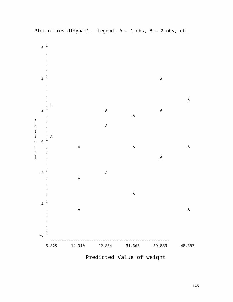
Selecting and Comparing Alternative Models
Process to Fit an Equation using Least Squares
Steps (same as for SLR):
3. Sample data are needed, on which the dependent variable
and all explanatory (independent) variables are
measured.
4. Make any transformations that are needed to meet the
most critical assumption: The relationship between y
and x’s is linear.
Example: volume = 0 + 1 dbh +2 dbh2 may be linear
whereas volume versus dbh is not. Need both variables.
3. Fit the equation to minimize the sum of squared error.
4. Check Assumptions. If not met, go back to Step 2.
5. If assumptions are met, then check if the regression is
significant. If it is not, then it is not a candidate model
(need other x-variables). If yes, then go through further
steps for MLR.
145

6. Are all variables needed? If there are x-variables that are
not significant, given the other variables:
drop the least significant one (highest p-value, lowest F,
or lowest absolute value of t)
refit the regression and check assumptions.
if assumptions are met, then repeat steps 5 and 6
continue until all variables in the regression are significant
given the other x-variables also in the model
146
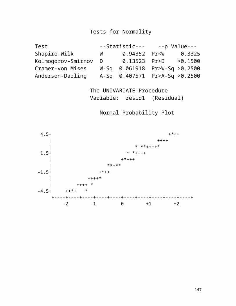
Methods to aid in selecting predictor (x) variables
Methods have been developed to help in choosing which x-
variables to include in the equation. These include:
1. R2 (or Adjusted R2). The equation is fitted for a number
of combinations of the x-variables to predict y. The ones
with the highest R2 are reported. CAUTION: You must
check the assumptions of these fitted equations by fitting
the equation with variables given. If assumptions are NOT
met, these are NOT candidate models EVEN with a high
R2. ALSO, consider costs of measuring the x-variables,
significance of the x-variables (given the other varables)
etc. This only gives some ideas of models to try.
147

2. Stepwise.
1) The most important variable is added to the model
(highest partial F-value or absolute value of t; has lowest
p-value).
2) Each of the other variables are added; the next most
important variable is added to the model
3) Repeat Step 2)
4) At any time, a variable already entered in, may become
not significant. Drop it, and continue with Step 2.
5) Continue until all variables in the regression are
significant, and the ones that are not in the equation are
not significant, given the ones that are in the equation.
NOTES:
This just gives candidate models. You must check
whether the assumptions are met and do a full
assessment of the regression results
148

3. Backwards Stepwise:
1) All x-variables are added to the model
2) Check to see if variables are not significant given the
other variables in the equation (use partial F-test or t-test)
3) If all x-variables are significant given the other variables,
stop. Otherwise, drop the variable with the lowest partial
F-value (highest p-value)
4) Repeat step 2, until all variables in the equation are
significant, given the other variables that are in the equation
NOTES:
This again just gives candidate models. You must
check whether the assumptions are met and do a full
assessment of the regression results
Unlike “stepwise”, once a variable is dropped, it
cannot come back in, even if it might be significant
with a different set of x-variables than when it was
dropped.
149

4. Forward Stepwise: This is the same as Stepwise,
EXCEPT, that once a x-variable is added to the model, it is
not removed, even if it becomes non-significant at a
particular step in the process.
NOTES:
This again just gives candidate models. You must
check whether the assumptions are met and do a full
assessment of the regression results
[See example]
150

Steps for Forward Stepwise, for example:
To fit this “by hand”, you would need to do the following steps:
1. Fit a simple linear regression for vol/ha with each of the explanatory (x) variables.
2. Of the equations that are significant (assumptions met?), select the one with the highest F-value.
3. Fit a MLR with vol/ha using the selected variable, plus each of the explanatory variables (2 x-variables in each equations). Check to see if the “new” variable is significant given the original variable (which may now be not significant, but forward stepwise does not drop variables). Of the ones that are significant (given the original variable is also in the equation), pick the one with the largest partial-F (for the new variable).
4. Repeat step 3, bringing in varables until i) there are no more variables or ii) the remaining variables are not significant given the other variables.
151

SAS code*MLR_stepwise.sas example for 430 and 533 classes ;* NOTE: Must run a full regression on your selected models once after using these tools to help you choose a few candidates;
PROC IMPORT OUT= WORK.voldata DATAFILE= "E:\frst430\lemay\examples\MLR.XLS" DBMS=EXCEL REPLACE; SHEET="data$"; GETNAMES=YES; MIXED=NO; SCANTEXT=YES; USEDATE=YES; SCANTIME=YES;RUN;options ls=70 ps=50 pageno=1;run;*------forward stepwise--------------;title 'forward stepwise';PROC REG data=voldata simple; model volha=baha stemsha qdbh age si topht/selection=forward; output out=out1 p=yhat1 r=resid1;run;
152

* keep first 3 variables, then forward stepwise;title 'first 3 then forward';PROC REG data=voldata; forward3: model volha=baha stemsha qdbh age si topht/selection=forward include=3; output out=out2 p=yhat2 r=resid2;run;*----------------------------------;* backward stepwise;title 'backward';PROC REG data=voldata; model volha=baha stemsha qdbh age si topht/selection=backward; output out=out3 p=yhat3 r=resid3;run;*------------------------------------;* stepwise –bring variables in or out;title 'stepwise – can bring variables in or out';PROC REG data=voldata; model volha=baha stemsha qdbh age si topht/selection=stepwise; output out=out4 p=yhat4 r=resid4;run;
153

*-------------------------------------;
* use rsquare to get a number of regressions ;title 'rsquare';PROC REG data=voldata; model volha=baha stemsha qdbh age si topht/selection=rsquare;run;
154

SAS Outputs:
forward stepwise
The REG Procedure
Number of Observations Read 28 Number of Observations Used 28
Descriptive Statistics Uncorrected Variable Sum Mean SS VarianceIntercept 28.00000 1.00000 28.00000 0baha 1023.60000 36.55714 39443 74.93884stemsha 65816 2350.57143 213051770 2160984qdbh 476.80000 17.02857 9084.32000 5.74434age 2028.00000 72.42857 176972 4.32804si 422.90000 15.10357 6594.19000 7.66258topht 549.60000 19.62857 11022 8.66878volha 14995 535.53929 9011680 36341
Descriptive Statistics
StandardVariable Deviation LabelIntercept 0 Interceptbaha 8.65672 bahastemsha 1470.02848 stemshaqdbh 5.97866 qdbhage 33.38155 agesi 2.76814 sitopht 2.94428 tophtvolha 190.63388 volha
155

The REG Procedure Model: MODEL1 Dependent Variable: volha volha
Number of Observations Read 28 Number of Observations Used 28
Forward Selection: Step 1
Variable baha Entered: R-Square = 0.7713 and C(p) = 387.3512
Analysis of Variance
Sum of MeanSource DF Squares Square F Value Pr > F
Model 1 756843 756843 87.70 <.0001Error 26 224372 8629.69076Corrected Total 27 981214
Parameter Standard Type II FVariable Estimate Error SS Value Pr>FIntercept -171.49367 77.51211 42243 4.90 .0359baha 19.34049 2.06520 756843 87.70 <.0001
Bounds on condition number: 1, 1
156

Forward Selection: Step 2
Variable topht Entered: R-Square = 0.9852 and C(p) = 4.5439
Analysis of Variance
Sum of MeanSource DF Squares Square F Value Pr > F
Model 2 966736 483368 834.64 <.0001Error 25 14478 579.13628Corrected Total 27 981214
Parameter Standard Type FVariable Estimate Error II SS Value Pr> F
Intercept -663.29189 32.71936 238002 410.9 <.0001baha 15.73874 0.56747 445489 769.23 <.0001topht 31.76327 1.66846 209894 362.43 <.0001
Bounds on condition number: 1.1251, 4.5002
157

Forward Selection: Step 3
Variable stemsha Entered: R-Square = 0.9879 and C(p) = 1.6949
Analysis of Variance
Sum of MeanSource DF Squares Square F Value Pr > F
Model 3 969381 323127 655.35 <.0001Error 24 11834 493.06283Corrected Total 27 981214
Parameter Standard TypeVariable Estimate Error II SS F Value Pr> F
Intercept-537.86686 62.00085 37107 75.26 <.0001baha 16.37897 0.59209 377309 765.24 <.0001stemsha -0.01319 0.00569 2644.90 5.36 0.0294topht 25.76009 3.01468 36001 73.02 <.0001
Bounds on condition number: 4.3142, 28.766--------------------------------------------------
No other variable met the 0.5000 significance level for entry into the model.
158

Summary of Forward Selection
Step Number Partial Model Vars In R-Square R-Square C(p) F Value1 baha 1 0.7713 0.7713 387.351 87.702 topht 2 0.2139 0.9852 4.5439 362.433 stemsha 3 0.0027 0.9879 1.6949 5.36
Summary of Forward Selection
Step Pr > F 1 <.0001 2 <.0001 3 0.0294
159

rsquare
The REG Procedure Model: MODEL1 Dependent Variable: volha R-Square Selection Method
Number of Observations Read 28 Number of Observations Used 28
Number in Model R-Square Variables in Model 1 0.7713 baha 1 0.5312 topht 1 0.3624 age 1 0.2847 qdbh 1 0.1936 stemsha 1 0.0833 si ------------------------------------------- 2 0.9852 baha topht 2 0.9512 baha stemsha 2 0.9501 baha qdbh 2 0.8946 baha age
. . .
5 0.9883 baha stemsha age si topht 5 0.9881 baha stemsha qdbh si topht 5 0.9880 baha stemsha qdbh age topht 5 0.9854 baha qdbh age si topht 5 0.9764 baha stemsha qdbh age si 5 0.6568 stemsha qdbh age si topht -------------------------------------------------- 6 0.9883 baha stemsha qdbh age si topht
160

Questions:
1. What was the final equation for each of the types of stepwise (or R square) methods?
2. Which equations would you choose to fit based on these tools to select variables? (full regression output would be needed in order examination of the residual plot and normality plot, R2 and SEE, significance of the regression, significance of the variables, cost/biology of the model)
161

For a number of models, select based on:
1. Meeting assumptions: If an equation does not meet
the assumption of a linear relationship, it is not a
candidate model
2. Compare the fit statistics. Select higher R2 (or I2), and
lower SEE (or SEE’)
3. Reject any models where the regression is not
significant, since this model is no better than just using
the mean of y as the predicted value.
4. Select a model that is biologically tractable. A simpler
model is generally preferred, unless there are
practical/biological reasons to select the more complex
model
5. Consider the cost of using the model
162
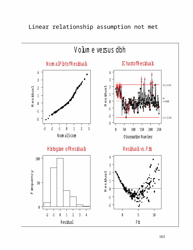
Adding class variables as predictors
(class variables as the dependent variable – covered in FRST 530; under generalized linear model—see also Chapter 14 in the textbook).
Want to add a class variable. Examples:
1. Add species to an equation to estimate tree height.
2. Add gender (male/female) to an equation to estimate
weight of adult tailed frogs.
3. Add machine type to an equation that predicts lumber
output.
163

How is this done?
Use “dummy” or “indicator variables to represent the class variablee.g. have 3 species. Set up X1 and X2 as dummy variables:
Species X1 X2 Cedar 1 0 Hemlock 0 1 Douglas fir 0 0o Only need two dummy variables to
represent the three species.o The two dummy variables as a
group represent the species. Add the dummy variables to the equation –
this will alter the intercept
164

To alter the slopes, add an interaction between dummy variables and continuous variable(s)e.g. have 3 species, and a continuous variable, dbh
Species X1 X2 X3=dbh X4=X1 * dbh X5=X2*dbh
Cedar 1 0 10 10 0 Hemlock 0 1 22 0 22 Douglas fir 0 0 15 0 0NOTE: There would be more than one line of data (sample) for each species.
o The two dummy variables, and the interactions with the continuous variable as a group represent the species.
165

166

How does this work?
For Cedar (CW):
For Hemlock (HW):
For Douglas fir (FD):
Therefore: fit one equation using all data, but get
different equations for different species. Also, can test
for differences among species, using a partial-F test.
167
* class_variables.sas ---------------;
options ls=70 ps=50 pageno=1;
PROC IMPORT OUT= WORK.trees DATAFILE= "E:\frst430\lemay\examples\diversity_plots.xls" DBMS=EXCEL REPLACE; SHEET="Data$"; GETNAMES=YES; MIXED=NO; SCANTEXT=YES; USEDATE=YES; SCANTIME=YES;RUN;
data trees2;set trees; if (tree_cls eq 'D') then delete; if ((species ne 'FD') and (species ne 'CW') and (species ne 'HW')) then delete;
* two dummies for 3 species;x1=0;x2=0;if species eq 'CW ' then x1=1;if species eq 'HW' then x2=1;* all dummies are zero for Douglas-fir;
x3=log10(dbh);x4=dbh;y=log(ht);
x5=x1*x3;
168

x6=x2*x3;x7=x1*x4;x8=x2*x4;run;proc sort data=trees2;by species;run;
proc plot data=trees2; plot ht*dbh=species;run;
proc plot data=trees2; plot ht*dbh=species; by species;run;
*-------------------------------------------;* full model with intercept and slope varying by species;proc reg; Full: model y=x1-x8; output out=out1 p=yhat1 r=resid1;run;
PROC PLOT DATA=out1; plot resid1*yhat1=species;run;
PROC univariate data=out1 plot;Var resid1;Run;
169

*-------------------------------------------;* reduced model with one common equation regardless of species;proc reg; Common: model y=x3 x4; output out=out2 p=yhat2 r=resid2;run;
PROC PLOT DATA=out2; plot resid2*yhat2=species;run;
PROC univariate data=out2 plot;Var resid2;Run;
*-------------------------------------------;* reduced model with common slopes for all species, but different intercepts;proc reg; INTONLY:model y=x1-x4; output out=out3 p=yhat3 r=resid3; run;
proc plot data=out3; plot resid3*yhat3=species;run;
PROC univariate data=out3 plot;Var resid3;Run;
170
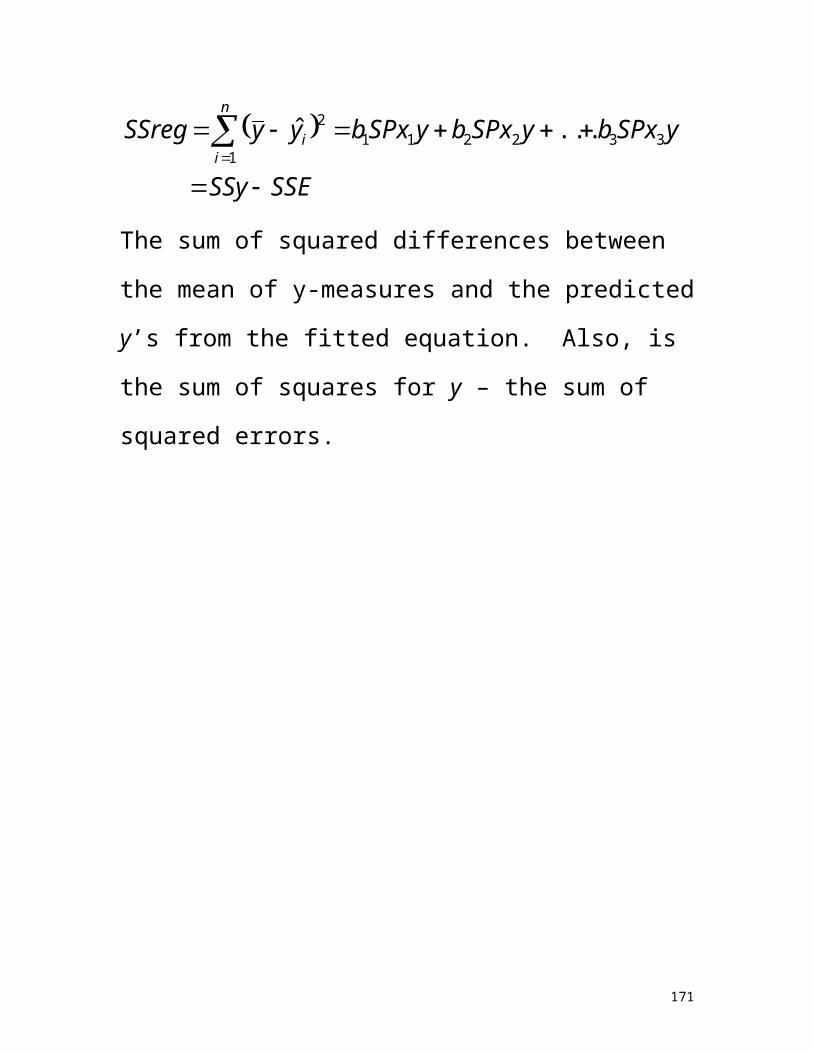
Plot of ht*dbh. Symbol is value of species.
‚ ‚ 70 ˆ ‚ ‚ F ‚ F ‚ 60 ˆ FF F F F F ‚ ‚ F F F F F F ‚ F F F F F FF ‚ HHHHHHH HH H F F FF 50 ˆ H HHHHHHHHH HH FF C ‚ HHHHHHHHHHH HH H H F ‚ H HHHHHHH HFCH F F ‚ HH HHHHHHHCFHHFHC FHFFCF F F C ‚ HHHH HH H HFFHCFHH FFFCFC C C 40 ˆ HHHH HHH HHHHCFFFFFF C FC F Ch ‚ H HHHHHHH FFFFFFFCFFFH FF CCC Ct ‚ HHHHHHHFF CFHCCFFFFCCH F HHC C C C C ‚ HHHHH FCFFFCCFFCHCCFFFCH CCCC ‚ HHHHHFCCCFCFCCFCCCCCCCCCC C 30 ˆ HHHHHHHHHCHCFCCCFCCCCF CC ‚ HHHH HCHCCFCCCCCCCCCCCF C ‚ HHHHHF CCCCCCCCCC CC CC F ‚ HHHHHFCCFCCCCCCCCCC ‚ HHHCCCCCCCCCCC C 20 ˆ HCHFCCCCCFC C ‚ HHHCFCCCC C F C ‚ HHFCCCCC HC FFH ‚ HHFCCCCCFCF ‚ HFCCCCC C 10 ˆ HFCCCC C ‚ FCCC F ‚ FCCCH C ‚ CCF F ‚ CC 0 ˆ ‚ Šˆ--------ˆ--------ˆ--------ˆ--------ˆ--------ˆ--------ˆ--------ˆ 0.0 26.1 52.2 78.3 104.4 130.5 156.6 182.7
dbhNOTE: 1284 obs hidden.
171

--------- species=CW --------------------
Plot of ht*dbh. Symbol is value of species.
‚ 50 ˆ ‚ C ‚ ‚ C ‚ C C ‚ C C C C ‚ C CCC C 40 ˆ C C C ‚ C CC ‚ C C C ‚ C CC C C C C C C ‚ C CC CC C CCC ‚ C CCCCCCCCC C ‚ C CCCCCCCCC 30 ˆ CCCCCCCCC CC ‚ C CCCCCCCC h ‚ CC CCCCCCCC C t ‚ CCCCCCCCC C ‚ CCCCCCCCC ‚ CCCCCCCC C ‚ CCCCCC C C 20 ˆ CCCCC C ‚ C CCC C ‚ CCC C ‚ CCC C ‚ CCC C ‚ CCC ‚ CCC C 10 ˆ CCCC ‚ CC ‚ CCC ‚ CC C ‚ C ‚ C ‚ 0 ˆ Š--ˆ-----------ˆ-----------ˆ-----------ˆ-----------ˆ-- 0 50 100 150 200
dbh
NOTE: 411 obs hidden.
172

---------------species=FD ------------------
Plot of ht*dbh. Symbol is value of species.
‚ 70 ˆ ‚ ‚ F ‚ F ‚ 60 ˆ F F F FF ‚ ‚ F F FF F F ‚ F FF F FF ‚ FFFF 50 ˆ FF ‚ F ‚ F FFF ‚ F F FF F FF ‚ FFFF FFF 40 ˆ FFFFF F F h ‚ FFFFFFFFFFF t ‚ FF FFFFFF F ‚ FFFFFFF FFF ‚ F FFFFF F 30 ˆ FFFF F F ‚ F FFF F F F ‚ FFFFF F F ‚ FFFFFF ‚ FFFF F 20 ˆ FFFFF ‚ FFFFF F ‚ FFFF F ‚ FFF FF ‚ FFFFF 10 ˆ FF F ‚ FFF F ‚ FFF ‚ FFFF ‚ FF 0 ˆ Š--ˆ-----------ˆ-----------ˆ-----------ˆ-----------ˆ-- 0 50 100 150 200
dbh
NOTE: 319 obs hidden.
173

------ species=HW --------------------------
Plot of ht*dbh. Symbol is value of species.
60 ˆ ‚ ‚ ‚ ‚ ‚ H HHHH HHHH HHH H H H HH 50 ˆ HHHHHHHHHH H H H HHH ‚ HHHHHHHHHHHHHHHHH H HHH H H ‚ H HHHHHHHH HHHH H H ‚ H HH HH H HH HH H H H H H ‚ HHH H HHH HHHHH H ‚ H H HH HH H H HHH HH HH H 40 ˆ HH H HH HHH H HHH H H H ‚ H H H HHHH H H H H HH HH H H ‚ H HH H HHHHH H H HHHHHHHHHHHHHH H H H H ‚ HH H HHHH HHH HH H H HH ‚ H H H H H H H H H Hh ‚ HH HHHH HH H HHH H H H Ht 30 ˆ H H HH H H HH HHHH HH HH ‚ HHHHHH H HHH HHHHHHHH HH H H ‚ HH HHHH H H HHHHHHHHHHH HH ‚ H HHH H HH H HH H HH ‚ HH H H H HHH HHHHHHHH ‚ HHHH H H H 20 ˆ H H HHH H ‚ HHHH HH HH H H H ‚ HH H H HHH H ‚ HHHHHH H HH H ‚ HHH HHHHHHHH ‚ HH HHHHH HH 10 ˆ HHHHHHHH ‚ H HHHH H ‚ HHHHH H ‚ HHHHH ‚ HHH ‚ HH 0 ˆ Š-ˆ---------ˆ---------ˆ---------ˆ---------ˆ---------ˆ---------ˆ-- 2 17 32 47 62 77 92
dbh
174

The REG Procedure Model: Full Dependent Variable: y
Number of Observations Read 1725 Number of Observations Used 1725
Analysis of Variance
Sum of Mean Source DF Squares Square F Value Pr > F
Model 8 688.80495 86.10062 1274.68 <.0001 Error 1716 115.91051 0.06755 Corrected Total 1724 804.71546
Root MSE 0.25990 R-Square 0.8560Dependent Mean 3.09332 Adj R-Sq 0.8553Coeff Var 8.40191
Parameter Estimates
Parameter StandardVariable DF Estimate Error t Value Pr > |t| Intercept 1 0.52420 0.05782 9.07 <.0001x1 1 -0.37609 0.09275 -4.05 <.0001x2 1 -0.37207 0.08463 -4.40 <.0001x3 1 1.80625 0.05491 32.89 <.0001x4 1 -0.00239 0.00070334 -3.40 0.0007x5 1 0.29106 0.08800 3.31 0.0010x6 1 0.98797 0.08989 10.99 <.0001x7 1 -0.00524 0.00117 -4.46 <.0001x8 1 -0.02160 0.00158 -13.67 <.0001
175

The REG Procedure Model: Common Dependent Variable: y
Number of Observations Read 1725 Number of Observations Used 1725
Analysis of Variance
Sum of Mean Source DF Squares Square F Value Pr > F
Model 2 606.66176 303.33088 2637.34 <.0001 Error 1722 198.05370 0.11501 Corrected Total 1724 804.71546
Root MSE 0.33914 R-Square 0.7539Dependent Mean 3.09332 Adj R-Sq 0.7536Coeff Var 10.96352
Parameter Estimates
Parameter Standard Variable DF Estimate Error t Value Pr > |t|
Intercept 1 0.45235 0.04517 10.01 <.0001 x3 1 2.05848 0.04409 46.69 <.0001 x4 1 -0.00825 0.00064234 -12.84 <.0001
176

Summary:
Assumptions met?
Full:Common:Intercept Only:
R Square and SE E
Full:Common:Intercept Only:
Df, SSR, SSE:
Model dfmodel
SSR dferror
SSE
Full
Common
Int. Only
177

Full versus Common
HO: Equations are the same for all speciesH1: Equations differ
Partial F:
Compare to:
F distribution for a 1- α percentile with r and n-m-1 (full
model) degrees of freedom.
Decision:
If equations differ – could we use the same slope, just different intercepts?
178

Full versus Intercepts only models
HO: Slopes are the same for all species H1: Slopes differ
Partial F:
Compare to:
Decision:
179

Modifications:
More than 3 species:
More than 1 continuous variable:
180
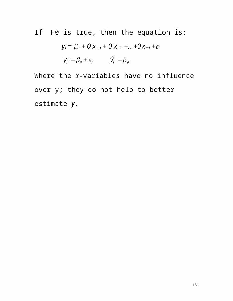
Experimental Design
Sampling versus experiments
similar to sampling and inventory design in that
information about forest variables is gathered and
analyzed
experiments presuppose intervention through applying a
treatment (an action or absence of an action) to a unit,
called the experimental unit. The experimental unit is an
item on which the treatment is applied.
The goal is to obtain results that indicate cause and
effect.
181

Definitions of terms and examples
For each experimental unit, measures of the variables of
interest (i.e., response or dependent variables) are used
to indicate treatment impacts.
Treatments are randomly assigned to the experimental
units.
Replication is the observation of two or more
experimental units under identical experimental
conditions.
A factor is a grouping of related treatments.
182

Examples:
1. 1,000 seedlings in a field. Half of the seedlings get a
“tea bag” of nutrients, others do not, randomly assigned.
Experimental unit: the seedling.
Treatments are: no tea bag, and tea bag.
Factor: only one – fertilizer (none, tea bag)
Replications: 500 seedlings get each treatment
2. 300 plant pots in a greenhouse: Each plant gets either 1)
standard genetic stock; 2) genetic stock from another
location; 3) improved genetic stock.
Treatments:
Experimental Unit:
Factor(s):
Replications:
183

3. The number of tailed frogs in different forest types is of
interest. There are six areas. Three are cut and the other
three are not cut.
Treatments:
Experimental Unit:
Factor(s):
Replications:
4. Two forest types are identified, Coastal western
hemlock and interior Douglas fir. For each, a number of
samples are located, and the growth of each tree in each
sample is measured.
Treatments:
Experimental Unit:
Factor(s):
Replications:
184

5. The effect of animal browsing on herbaceous plants is
of interest. In each of two forest types, 10 areas are
established at the beginning of the year. Five out of the
10 are fenced off, eliminating animal browsing. The rest
are marked but left open to animals. The heights and
coverages of plants are measured at the end of the year.
Treatments:
Experimental Unit:
Factor(s):
Replications:
Randomization?
185
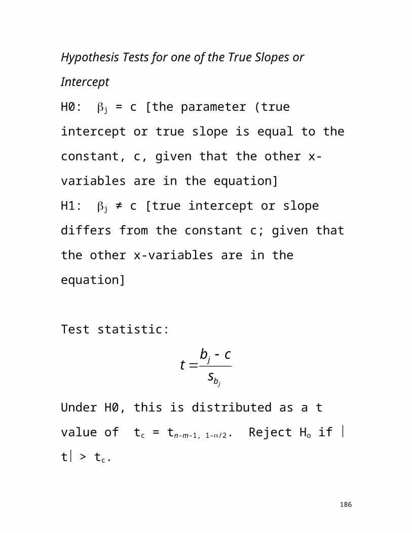
What is treatments are randomly assigned to experimental
units?
Haphazard vs. random allocation
Practical problems and implications
Other terms:
The null hypothesis is that there are no differences
among the treatment means. For more than one factor,
there is more than one hypothesis
The sum of squared differences (termed, sum of squares)
between the average for the response variable by
treatment versus the average over all experimental units
represents the variation attributed to a factor.
The degrees of freedom, associated with a factor, are the
number of treatment levels within the factor minus one.
186

Example:
Factor A, fertilizer: none, medium, heavy (3 levels)
Factor B, species: spruce, pine (2 levels)
Number of possible treatments: 6 e..g, spruce, none is one
treatment.
Experimental Unit: 0.001 ha plots
Replicates planned: 2 per treatment (cost constraint). How
many experimental units do we need?
Variable of interest: Average 5-year height growth for trees in
the plot
Null hypotheses:
There is no different between the 6 treatments. This can be
broken into:
1) There is no interaction between species and fertilizer.
2) There is no difference between species.
3) There is no difference between fertilizers.
187

Experimental error is the measure of variance due to
chance causes, among experimental units that received
the same treatment.
The degrees of freedom for the experimental error relate
to the number of experimental units and the number of
treatment levels.
The impacts of treatments on the response variables will
be detectable only if the impacts are measurably larger
than the variance due to chance causes.
To reduce the variability due to causes other than those
manipulated by the experimenter, relatively homogenous
experimental units are carefully selected.
188

Random allocation of a treatment to an experimental unit
helps insure that the measured results are due to the
treatment, and not to another cause.
Example: if we have applied the no fertilizer treatment to
experimental units on north facing sites, whereas moderate
and heavy fertilizer treatments are applied only to south
facing sites, we would not know if differences in average
height growth were due to the application of fertilization,
the orientation of the sites, or both. The results would be
confounded and very difficult to interpret.
189

Variations in experimental design
Introduction of More Than One Factor:
Interested in the interaction among factors, and the effect
of each factor.
A treatment represents a particular combination of levels
from each of the factors.
When all factor levels of one factor are given for all
levels of each of the other factors, this is a crossed
experiment. Example: two species and three fertilization
levels = six treatments using a crossed experiment.
190
Fixed, Random, or Mixed Effects:
Fixed factors: the experimenter would like to know the
change that is due to the particular treatments applied;
only interested in the treatment levels that are in the
experiment (e.g., difference in growth between two
particular genetic stocks) [fixed effects]
Random factors: the variance due to the factor is of
interest, not particular levels (e.g., variance due to
different genetic stocks—randomly select different stock
to use as the treatment) [random effects]
Mixture of factor types: Commonly, experiments in
forestry include a mixture of factors, some random and
some fixed [mixed effect].
191

Restricted Randomization Through Blocking: Randomized
Block (RCB), Latin Square, and Incomplete Blocks
Designs:
Randomize treatments with blocks of experimental units
Reduces the variance by taking away variance due to the
item used in blocking (e.g., high, medium and low site
productivity
Results in more homogeneous experimental units within
each block.
192

Restricted Randomization Through Splitting Experimental
Units:
Called “split plot”
An experimental unit is split. Another factor is randomly
applied to the split.
Example: The factor fertilizer is applied to 0.001 ha plots.
Each of the 0.001 ha plot is then split into two, and two
different species are planted in each. Fertilizer is applied to
the whole plot, and species is applied to the split plot.
Species is therefore randomly assigned to the split plot, not
to the whole experimental unit.
193

Nesting of Factors
Treatment levels for one factor may be particular to the
level of another factor, resulting in nesting of treatments.
Example, for the first level of fertilizer, we might use
medium and heavy thinning, whereas, for the second level
of fertilizer, we might use no thinning and light thinning.
194

Hierarchical Designs and Sub-Sampling:
Commonly in forestry experiments, the experimental
unit represents a group of items that we measure. E.g.
several pots in a greenhouse, each with several plants
germinating from seeds.
Treatments are randomly assigned to the larger unit (e.g,
to each plot not to each seedling). The experimental unit
is the larger sized unit.
May want variance due to the experimental unit (pots in
the example) and to units within (plants in the example).
These are 1) nested in the treatment; 2) random effects;
and 3) hierarchical
A common variation on hierarchical designs is
measuring a sample of items, instead of measuring all
items in an experimental unit.
195

Introduction of Covariates
The initial conditions for an experiment may not be the
same for all experimental units, even if blocking is used
to group the units.
Site measures such as soil moisture and temperature, and
starting conditions for individuals such as starting height,
are then measured (called covariates) along with the
response variable
These covariates are used to reduce the experimental
error.
Covariates are usually interval or ratio scale
(continuous).
196

Designs in use
The most simple design is one fixed-effects factor, with
random allocation of treatments to each experimental
unit, with no 1) blocking; 2) sub-sampling; 4) splits; or
5) covariates
Most designs use combinations of the different
variations. For example, one fixed-effects factor, one
mixed-effects factor, blocked into three sites, with trees
measured within plots within experimental units (sub-
sampling/hierarchical), and measures taken at the
beginning of the experiment are used as covariates (e.g.,
initial heights of trees.
197

Why?
Want to look at interactions among factors and/or is
cheaper to use more than one factor in one experiment
than do two experiments.
Experiments and measurements are expensive – use
sampling within experimental units to reduce costs
Finding homogeneous units is quite difficult: blocking is
needed
BUT can end up with problems: some elements are not measured, random allocation is not possible, or measures are correlated in time and/or space.
In this course, start with the simple designs and add complexity.
198

Main questions in experiments
Do the treatments affect the variable of interest?
For fixed effects: Is there a different between the treatment
means of the variable of interest? Which means differ?
What are the means by treatment and confidence intervals
on these means?
For random effects: Do the treatments account for some of
the variance of the variables of interest? How much?
199

Completely Randomized Design (CRD)
Homogeneous experimental units are located
Treatments are randomly assigned to treatment units
No blocking is used
We measure a variable of interest for each
experimental unit
CRD: One Factor Experiment, Fixed Effects
REF: Ch. 16, 17, 18 of Neter et al.
Main questions of interest
Are the treatment means different?
Which means are different?
What are the estimated means and confidence intervals for
these estimates?
200

Notation:
Population: OR ijjijy
ijy = response variable measured on experimental unit i and treatment j
j=1 to J treatments
= the grand or overall mean regardless of treatment
= the mean of all measures possible for treatment j
j = the difference between the overall mean of all measures possible from all treatments and the mean of all possible measures for treatment j, called the treatment effect
ij = the difference between a particular measure for an experimental unit i, and the mean for the treatment j that was applied to it
jijij y
201

For the experiment:
ijjij eyy OR ijjij eyy
y = the grand or overall mean of all measures from the experiment regardless of treatment; under the assumptions for the error terms, this will be an unbiased estimate of
jy = the mean of all measures for treatment j; under the assumptions for the error terms, this will be an unbiased estimate of
j = the difference between the mean of experiment measures for treatment j and the overall mean of measures from all treatments; under the error term assumptions, will be an unbiased estimate of j
ije = the difference between a particular measure for an experimental unit i, and the mean for the treatment j that was applied to it
jijij yye nj = the number of experimental units measured in treatment j
nT = the number of experimental units measured over all
treatments =
J
jjn
1
202

Example: Fertilization Trial
A forester would like to test whether different site preparation methods result in difference in heights. Fifteen areas each 0.02 ha in size are laid our over a fairly homogeneous area. Five site preparation treatments are randomly applied to 25 plots. One hundred trees are planted (same genetic stock and same age) in each area. At the end of 5 years, the heights of seedlings in each plot were measured, and averaged for the plot.
i = a particular 0.02 ha area in treatment j, from 1 to 5.Response variable ijy : 5-year height growth (one average for each experimental unit)
Number of treatments: J=5 site preparation methods
nT = the number of experimental units measured over all
treatments =
5
1jjn =25
n1 = n2 =n3 =n4 =n5 =5 experimental units measured each treatment
203

Schematic of Layout:3 4 4 5 11 2 3 5 22 1 2 4 25 4 3 1 54 3 1 5 3
Data Organization and Preliminary Calculations
For easy calculations by hand, the data could be organized in a spreadsheet as:
Obs:Treatment, j=1 to J
i=1 to nj 1 2 3 … J1 y11 y12 y13 … y1J
2 y21 y22 y23 … y2J
3 y31 y32 y33 … y3J
… … … … … …n yn1 yn2 yn3 … ynJ
Sum y.1 y.2 y.3 … y.J y..Averages
1y 2y 3y Jy y
1 11 T
J
i
n
iij
j
jj
n
iijj n
yyyyny
yyyjj
NOTE: may not be the same number of observations for each treatment.
204

Example:
J= 5 site preparation treatments randomly applied to n=25 plots.
Response Variable: Plot average seedling height after 5 years
Plot Average Heights (m)
Treatments OverallObservation 1 2 3 4 5
1 4.6 4.9 4.0 3.4 4.32 4.3 4.3 3.7 4.0 3.73 3.7 4.0 3.4 3.0 3.74 4.0 4.6 3.7 3.7 3.05 4.0 4.3 3.0 3.4 3.4
SUMS 20.600 22.100 17.800 17.500 18.100 96.100Means 4.120 4.420 3.560 3.500 3.620 3.844nj 5 5 5 5 5 25
Example Calculations:
844.325/1.96)5.178.17...1.226.20(
12.45/)3.40.47.33.46.4(5
5
1
5
1 1
5
11
kj
j
n
iij
iij
n
yy
yy
j
205

We then calculate:
1) Sum of squared differences between the observed values
and the overall mean (SSy):
J
jj
J
j
n
iij ndfyySSy
j
11 1
2 1
Also called, sum of squares total (same as in regression)
2) Sum of squared differences between the treatment
means, and the grand mean, weighted by the number of
experimental units in each treatment (SSTR)
12
11 1
2
JdfyynyySSJ
jjj
J
j
n
ijTR
j
3) Sum of squared differences between the observed values for each experimental unit and the treatment means (SSE)
J
j
n
iTjij
j
JndfyySSE1 1
2
SSESSSSy TR
206

Alternative formulae for the sums of squares that may be easier to calculate are:
TR
T
J
jjjTR
T
J
j
n
iij
SSSSySSEnyynSS
nyySSy
j
2
1
2
2
1 1
2
207

For the example, differences from treatment means (m):
Treatments OverallObs. 1 2 3 4 5 1 0.480 0.480 0.440 -0.100 0.6802 0.180 -0.120 0.140 0.500 0.0803 -0.420 -0.420 -0.160 -0.500 0.0804 -0.120 0.180 0.140 0.200 -0.6205 -0.120 -0.120 -0.560 -0.100 -0.220 SUMS 0.000 0.000 0.000 0.000 0.000 0.000Sum of Squares Error 0.468 0.468 0.572 0.560 0.908 2.976nj 5 5 5 5 5 25s2j 0.117 0.117 0.143 0.140 0.227
Example Calculations:
468.0)1.40.4()1.40.4()1.47.3()1.43.4()1.46.4(
1for
22222
5
1
211
j
j yy treatmentSSE
117.015
468.01
1 for
1
12
ntreatmentSSEs
2.976 0.9080.5600.5720.4680.468 5 for SSE ...2 for SSE 1 for
1 1
2
treatmenttreatmenttreatmentSSE
yySSEJ
j
n
ijij
j
208

Differences from grand mean (m)
Treatments OverallObs. 1 2 3 4 5
1 0.756 1.056 0.156-
0.444 0.456
2 0.456 0.456-
0.144 0.156-
0.144
3-
0.144 0.156-
0.444-
0.844-
0.144
4 0.156 0.756-
0.144-
0.144-
0.844
5 0.156 0.456-
0.844-
0.444-
0.444
SUMS 1.380 2.880-
1.420-
1.720-
1.120 0.000Sum of Squares Total 0.849 2.127 0.975 1.152 1.159 6.262nj 5 5 5 5 5 25
6.262 1.1591.1520.97502.1270.849 5 for SSy ...2 for SSy 1 for
1 1
2
treatmenttreatmenttreatmentSSy
yySSyJ
j
n
iij
j
209
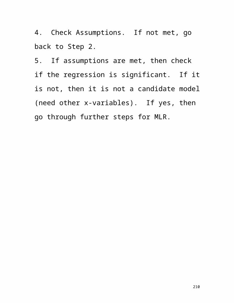
Difference between treatment means and grand mean (m)
Treatments Overall 1 2 3 4 5 Mean 4.120 4.420 3.560 3.500 3.620
Difference 0.276 0.576-
0.284-
0.344-
0.224 0.000Sum of Squares Treatment 0.076 0.332 0.081 0.118 0.050 3.286nj 5 5 5 5 5 25
Example Calculations:
286.3)844.3620.3(5)844.3500.3(5)844.3560.3(5
)844.3420.4(5)844.3120.4(5
222
22
1
2
J
jjjTR yynSS
210

Test for differences among treatment means
The first main question is: Are the treatment means different?
H0: 1 = 2 = … = J
H1: not all the sameOR:
H0: J 21
H1: not all equal to 0OR:
H0: (TR+ε) /ε = 1H1: (TR+ε)/ε > 1
Where ε is the variance of the error terms;
TR is the effect of the fixed treatments (see page 234 for
more details on what this is).
If the treatment does not account for any of the variance in
the response variable, then treatment effects are likely all =
0, and all the treatment means are likely all the same.
Using an analysis of variance table:
211

Source df SS MS F p-valueTreatment
J-1 SSTR MSTR=SSTR/(J-1)
F= MSTR/MSE
Prob F> F(J-1),( nT -J),
(1- α)
Error nT -J SSE MSE= SSE/(nT-J)
Total nT -1 SSy
MSEMS
JnSSEJSS
nSSE
JSSF TR
T
TRJ
jj
TR
)/()1/(
)1(/
)1/(
1
Under H0, and the assumptions of analysis of variance, this follows an F-distribution. If
)1,,1( JnJ TFF
We reject H0 and conclude that there is a difference between the treatment means.
Notice that this is a one-sided test, using 1-α
This is because we are testing if the ratio of variances is > 1.
212

For example, if we have 4 treatments, and 12 experimental units, and we want α=0.05:If the calculated F is larger than 4.07, we reject H0: The
treatments means are likely different, unless a 5% error has
occurred.
OR: We take our calculated F value from our experiment
and plot it on this F curve. Then, find the area to the right
of this value (p-value). We reject a hypothesis if the
probability value (p-value) for the test is less than the
specified significance level.
0 2.4 4.8
F(3,8; 0.95)=4.07
Rejection Region
213
For the example: If assumptions of ANOVA are met then interpret the F-value.
H0: μ1= μ2 =μ3 =μ4 =μ5
H1: not all equal
Analysis of Variance (ANOVA) Table:
Source df SS MS Fp-
valueTreatment 5-1=4 3.286 0.821 5.51 0.004
Error25-5=20 2.976 0.149
Total25-1=24 6.262
If assumptions of ANOVA are met then interpret the F-value. NOTE: Fcritical for alpha=0.05, df treatment=4 and df error=20 is 2.87.
Since the p-value is very smaller (smaller than alpha=0.05),
we reject H0 and conclude that there is a difference in the
treatment means. BUT this is only a good test if the
214

assumptions of analysis of variance have been met. Need
to check these first (as with regression analysis).
Assumptions regarding the error term
For the estimated means for this experiment to be unbiased
estimates of the means in the population, and the MSE to
be an unbiased estimate of the variance within each
experimental unit, the following assumptions must be met:
1. Observations are independent – not related in time nor
in space [independent data]
2. There is normal distribution of the y-values [or the
error terms] around each treatment mean [normally
distributed]
3. The variances of the y’s around each treatment mean
[or the error terms] are the same (homogeneous) for
all treatment means [equal variance]
215

Similar to regression:
a normal probability plot for the error terms can
be used to check the assumption of normality,
and
a residual plot can be used to visually check the
assumption of equal variance.
OR, these can be tested using (1) normality tests (as with
regression); (2) Bartlett’s test for equal variances (for more
than one factor or for other designs with blocking, etc. this
becomes difficult).
216

Transformations to meet assumptions
Similar to regression: logarithmic transformations can be used to equalize
variances arcsine transformation can be used to transform
proportions into normally distributed variables rank transformation can be used when data are not
normally distributed and other transformations do not “work” [nonparametric analysis of variance using ranks]
Unlike regression you must transform the y-variable
Process: do your analysis with the measured response variable if assumptions of the error term are not met, transform
the y-variable do the analysis again and check the assumptions; if not
me, try another transformation may have to switch to another method: generalized
linear models, etc.
217

Expected values:
Under the assumptions of analysis of variance, MSE is an
unbiased estimate of ε and MSTR is an unbiased estimate
of TR+ε. Therefore, this F-test will give the
correct probabilities under the assumptions.
This is the same as saying that the expected value of MSE
is ε , and the expected value of MSTR is TR+ε. The
F-test is then a measure of how much larger the value is
when the treatment means are accounted for.
218

For the example, before interpreting the ANOVA table, we must check assumptions of ANOVA:
Is there equal variance across treatments? (estimated by MSE as 0.149 on our ANOVA table). Using a residual plot and EXCEL:
Residual Plot
-0.8-0.6-0.4-0.20.00.20.40.60.8
3.2 3.4 3.6 3.8 4.0 4.2 4.4 4.6
4 3 5 1 2Pred. Values (Treat. Means in m)
Res
idua
ls (E
rror
in m
)
219

Are residuals normally distributed? Again using EXCEL:
Residuals vs. normal z(0,1)
0.00
0.20
0.40
0.60
0.80
1.00
-2 -1 0 1 2
z-values
Cum
ulat
ive
prob
abili
ty
Stand. Resz(0,1)
Where standardized residuals are calculated by:
MSEe
e ii
0)edstandardiz(
Compare these to z-values for a standard normal distribution with a mean of zero and a variance of 1 (z(0,1))
220

Differences among particular treatment means
If there are differences among means detected, which means differ?
Can use: Orthogonal contrasts – see textbook Multiple comparisons
Multiple comparisons (or contrasts):
Many different types, e.g.o T-test for every pair of means; must adjust the
alpha level used by dividing by the number of pairs.
o Scheffe’s multiple comparisonso Bonferonni’s adjustments
Try to “preserve” the alpha level used to test all the means together (the F-test)
221

For the example, given that there is a difference among treatment means, which pairs of means differ?
t-test for pairs of means: determine the number of pairs possible
means of pairs possible 10!2!3
!525
Comparing Treatments 2 (largest estimated mean) versus 4 (smallest estimated mean):
686.3
51
51149.0
)5.34.4(
11
0)(
0:H:H OR 0:H
42
42
421
420420
t
nnMSE
yyt
222

Under H0: This follows:
JnTt ,2/1
Using alpha=0.005 (0.05/10=0.005), for 5 treatments and 25 observations, the t-value is 3.153. Result?
Another way to assess this is to obtain the p-value for t=3.686, with 20 degrees of freedom (25-5).
This is 0.001464. Since this is less than 0.005, we reject H0
and conclude that these two means differ.
Can test the other pairs of means. could test for any size of difference between two
means, for example:
42
42
42
42
11
)(
:H1 :H0
nnMSE
cyyt
cc
223

Scheffe’s multiple comparison test – conservative
Can test any pair of means or other comparisons.
Testing whether the means for Treatments 2 and 4 differ:
4242
54321
:H0 021
21:H0
00210
210:H0
The test statistic is:
J
j jj
J
jjj n
cMSELsycLLsLS
1
2
1
1)ˆ(ˆ)ˆ(
ˆ
The sum of the cj values must add up to zero.
224

For this example:
686.3122.045.0
122.051
21
51
21149.0)ˆ(
45.05.3214.4
21ˆ
0210
210
22
54321
S
Ls
L
ccccc
Under H0, this follows:
JnJ TFJ ,1,1)1(
For J=5, alpha=0.05, and nT=25 observations:
38.387.2)15(
Calculated S > 3.38, so we reject H0, the treatment means differ. (NOTE: The means would have to be at least 0.826 apart to reject)
225

Scheffe’s can be used for many comparisons.
For example: Test if treatments 3, 4 and 5 differ from treatments 1 and 2:
032
:H0
OR031
31
31
21
21:H0
54321
54321
NOTE: c’s add up to 0.
30.4158.068.0
158.0)ˆ(
68.06.3315.3
316.3
314.4
211.4
21ˆ
31
31
31
21
21
54321
S
Ls
L
ccccc
Result: Greater than the critical value of 3.38; do reject H0.
158.051
31
51
31
51
31
51
21
51
21149.0)ˆ(
22222
Ls
226

Confidence limits for treatment means
Under the assumptions, confidence intervals for each treatment mean can be obtained by:
jJnj n
MSEtyT 21),(
Since MSE estimates the variance that is assumed to be
equal, and the observations are normally distribution and
independent.
For the example:
09.2
173.05149.0equalallareassametheAll
6.35.36.34.41.4
975.0,20
54321
21),(
t
nn
MSE
yyyyy
nMSEty
jj
jknj
For treatment 1:
)46.4,74.3(36.01.4173.009.21.4
227

Using SAS:
For entry into statistical programs like SAS, the data should be organized as:
Treatment Obs: Response
j=1 to J i=1 to nj
1 1 y11
1 2 y21
1 3 y31
… … …1 n1 y(n1) 1
2 1 y12
2 2 y22
2 3 y32
… … …2 n2 Y(n2) 2
… … …J 1 y1J
J 2 y2J
J 3 y3J
… … …J n J y(nJ) 3
228

For the example, we can put the data into an EXCEL file:
Treatment Observation AveHt1 1 4.61 2 4.31 3 3.71 4 4.01 5 4.02 1 4.92 2 4.32 3 4.02 4 4.62 5 4.33 1 4.03 2 3.73 3 3.43 4 3.73 5 3.04 1 3.44 2 4.04 3 3.04 4 3.74 5 3.45 1 4.35 2 3.75 3 3.75 4 3.05 5 3.4
229

* CRD.sas example for 430 and 533 classes ;PROC IMPORT OUT= WORK.htdata DATAFILE= "E:\frst430\lemay\examples\CRD_one_factor_no_sampling.XLS" DBMS=EXCEL REPLACE; SHEET="rawdata$"; GETNAMES=YES; MIXED=NO; SCANTEXT=YES; USEDATE=YES; SCANTIME=YES;RUN;
options ls=70 ps=50 pageno=1;run;
PROC GLM data=htdata;CLASS Treatment;MODEL aveht=treatment;MEANS treatment/scheffe hovtest=bartlett;estimate '1 VS others' treatment 4 -1 -1 -1 -1/divisor=4;OUTPUT OUT=GLMOUT PREDICTED=PREDICT RESIDUAL=RESID;RUN;
PROC PLOT DATA=GLMOUT;PLOT RESID*PREDICT='*';RUN;
PROC UNIVARIATE DATA=GLMOUT PLOT NORMAL;VAR RESID;RUN;
The GLM Procedure
230

Class Level Information
Class Levels Values Treatment 5 1 2 3 4 5
Number of Observations Read 25 Number of Observations Used 25
The GLM Procedure
Dependent Variable: AveHt AveHt
Sum of MeanSource DF Squares Square F Value
Model 4 3.28560000 0.82140000 5.52Error 20 2.97600000 0.14880000Corrected Total 24 6.26160000
Source Pr > F Model 0.0037 Error Corrected Total
R-Square Coeff Var Root MSE AveHt Mean
0.524722 10.03502 0.385746 3.844000
231

Source DF Type I SS Mean F Value Square Treatment 4 3.28560000 0.82140000 5.52
Source Pr > F Treatment 0.0037
Source DF Type III SS Mean Square F Value
Treatment 4 3.28560000 0.82140000 5.52
Source Pr > F Treatment 0.0037
The GLM Procedure
Bartlett's Test for Homogeneity of AveHt Variance
Source DF Chi-Square Pr > ChiSq
Treatment 4 0.5790 0.9654
232

The GLM Procedure
Scheffe's Test for AveHt
NOTE: This test controls the Type I experimentwise error rate.
Alpha 0.05Error Degrees of Freedom 20Error Mean Square 0.1488Critical Value of F 2.86608Minimum Significant Difference 0.826
Means with the same letter are not significantly different.
Scheffe Grouping Mean N Treatment
A 4.4200 5 2 A B A 4.1200 5 1 B A B A 3.6200 5 5 B B 3.5600 5 3 B B 3.5000 5 4
The GLM Procedure
Dependent Variable: AveHt AveHt
StandardParameter Estimate Error t Value Pr > |t|
1 VS others 0.34500000 0.19287302 1.79 0.0888
233
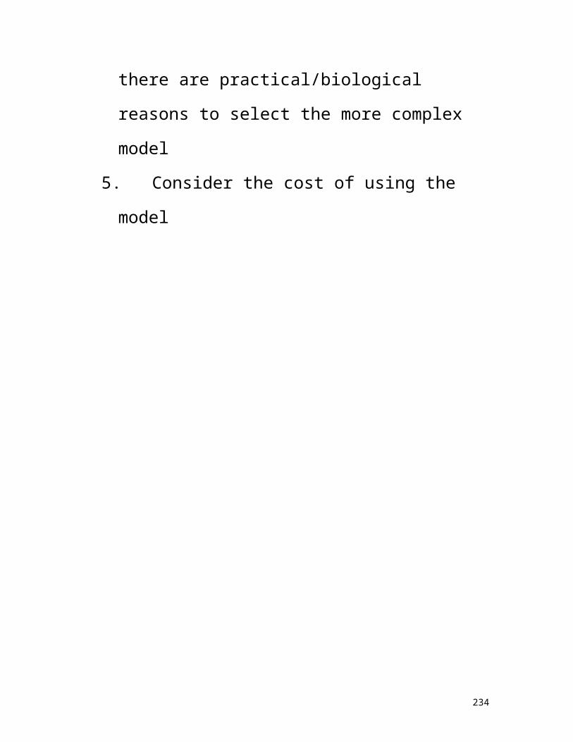
Plot of RESID*PREDICT. Symbol used is '*'.
RESID ‚ ‚ 0.8 ˆ ‚ ‚ * ‚ 0.6 ˆ ‚ ‚ * * * ‚ * 0.4 ˆ ‚ ‚ ‚ 0.2 ˆ * * * ‚ * ‚ * ‚ 0.0 ˆ ‚ ‚ * * * ‚ * -0.2 ˆ * ‚ ‚ ‚ -0.4 ˆ * * ‚ ‚ * ‚ * -0.6 ˆ * ‚ ‚ ‚ -0.8 ˆ ‚ Š-ˆ---------ˆ---------ˆ---------ˆ---------ˆ---------ˆ---------ˆ- 3.4 3.6 3.8 4.0 4.2 4.4 4.6
PREDICT
NOTE: 5 obs hidden.
234

The SAS System
The UNIVARIATE Procedure Variable: RESID
Moments
N 25 Sum Weights 25Mean 0 Sum Observations 0Std Deviation 0.35213634 Variance 0.124Skewness 0.0634775 Kurtosis -0.6323427Uncorrected SS 2.976 Corrected SS 2.976Coeff Variation . Std Error Mean 0.07042727
Basic Statistical Measures
Location Variability
Mean 0.00000 Std Deviation 0.35214Median -0.10000 Variance 0.12400Mode -0.12000 Range 1.30000Interquartile Range 0.34000
Tests for Location: Mu0=0
Test -Statistic- -----p Value------
Student's t t 0 Pr > |t| 1.0000Sign M -0.5 Pr >= |M| 1.0000Signed Rank S 2 Pr >= |S| 0.9584
235

Tests for Normality
Test --Statistic--- --p Value----
Shapiro-Wilk W 0.962795 Pr < W 0.4729Kolmogorov-Smirnov D 0.131787 Pr > D >0.1500Cramer-von Mises W-Sq 0.059919 Pr > W-Sq>0.2500Anderson-Darling A-Sq 0.370893 Pr > A-Sq >0.2500
The UNIVARIATE Procedure Variable: RESID
Quantiles (Definition 5)
Quantile Estimate 100% Max 0.68 99% 0.68 95% 0.50 90% 0.48 75% Q3 0.18 50% Median -0.10 25% Q1 -0.16 10% -0.50 5% -0.56 1% -0.62 0% Min -0.62
Extreme Observations
----Lowest---- ----Highest---
Value Obs Value Obs -0.62 24 0.44 11 -0.56 15 0.48 1 -0.50 18 0.48 6 -0.42 8 0.50 17 -0.42 3 0.68 21
236
Stem Leaf # Boxplot 6 8 1 | 4 4880 4 | 2 0 1 | 0 884488 6 +--+--+-0 6222200 7 *-----*-2 2 1 |-4 6022 4 |-6 2 1 | ----+----+----+----+ Multiply Stem.Leaf by 10**-1
The UNIVARIATE Procedure Variable: RESID
Normal Probability Plot 0.7+ ++*++ | * *+++*++ | ++*+++ | +***+** | **+*+* | +++*++ | ++*+*+* -0.7+ ++*++ +----+----+----+----+----+----+----+----+----+----+ -2 -1 0 +1 +2
237

Power of the Test:
A Type I error rate (α, significance level), the chance of
rejecting a null hypothesis when it is true (you reject when
the means are actually the same) must be selected. Given:
a particular number of experimental units
sizes of the differences between true population
means, and
variation within the experimental units
this will set the Type II error rate (β), the chance of
accepting a null hypothesis when it is false (you fail to
reject when the means are actually different)
The power of the test is 1- β, the probability you will
reject the null hypothesis and conclude that
there is a difference in means, when there IS a
difference between population means.
238

If the difference between population means (real treatment
means) is very large, than a small number of experimental
units will result in rejection of the null hypothesis.
If the number of experimental units is very large, then even
a small difference between population means will be
detected.
If the variation within experimental units is very small, then
the difference will be detected, even with a small difference
between population means, and even with only a few
treatment units.
239

Statistical Significance is not the same as differences of
Practical importance! UNLESS you:
have some idea of within experimental unit variation
from a previous study with the same conditions (e.g.,
MSE from a previous study)
know the size of the difference that you wish to detect
have selected the α level
Then:
You can calculate the number of experimental units per
treatment that will result in rejection of H0: when the
differences are that large or greater.
Alternatively:
You can calculate the power of the test for an experiment
you have already completed.
240

Power of the test for the example:
Have:
J=5 treatments, and df treatment is 5-1=4n=5 observations in each treatment, and df error is 25-5=20MSTR=0.821MSE=0.149 as an estimate of 2
Fcritical is F(0.95,4,20)=2.87
Also, E[MSTR ]=φTR+2
and E[MSTR ]= 2 .
538.0)149.0821.0(5
15ˆ
)(1ˆ
1
1
2
1
2
1
2
J
jj
TR
J
jj
jj
J
jj
TR
MSEMSn
Jthen
whereJ
n
241

Power is then Prob(F>Fcritical | Noncentral) where Noncentral is the noncentrality parameter, and for when H1 is true.
04.18149.0
538.05ˆ
21
2
noncentral
nnoncentral
J
jj
Then use SAS:
Data power;* Power=1-probf(Fcritical,df Treatment, df Error, Noncentral);Power=1-probf(2.87,4,20,18.04);Run;
The temporary file will have the result in it, which is 0.87. Often try to get power between 0.80 and 0.95.
242

Can do power analysis for a planned experiment using:
1. A estimate of the of the variance of the error. This
could be from a previous, similar experiment.
2. The differences between treatment means that are the
minimum required to be of practical importance.
Can then test for how many observations are needed so that
statistical differences also mean differences of practical
importance [See SAS code called
One_way_anova_power_using_min_differences.sas]
243

Methods based on maximum likelihood rather than least
squares
ML methods can be used when:
Treatments are random rather than fixed (more on this
later)
Transformations do not result in assumptions being
met
Your dependent variable is a count, or it is a binary
variable (e.g., yes or no; dead or alive; present or
absent)
[See text for a little on this, also FRST 530]
244

CRD: Two Factor Factorial Experiment, Fixed Effects
REF: Neter et al., Ch 19 and 20
Introduction
Treatments can be combinations of more than one factor
For 2-factor experiment, have several levels of Factor A
and of Factor B
All levels of Factor A occur for Factor B and vice versa
(called a Factorial Experiment, or crossed treatments)
Example:
Factor A, (three levels of fertilization: A1, A2, and A3)
Factor B (four species: B1, B2, B3 and B4)
Crossed: 12 treatments
Four replications per treatment for a total of 48
experimental units
Measured Responses: height growth in mm
245

Schematic and Measured Response for the Example:
A1B1=1
0
A3B2=2
5
A3B4=3
5
A2B2=2
3
A1B2=1
4
A2B3=2
4
A1B4=2
4
A2B2=2
2
A1B2=1
5
A2B4=2
8
A3B3=3
2
A3B2=2
5
A3B2=2
7
A1B4=2
3
A3B3=2
9
A3B2=2
6
A1B3=1
7
A1B1=1
1
A3B4=3
5
A1B2=1
3
A1B4=2
2
A1B1=1
1
A2B3=2
4
A3B3=3
0
A1B3=1
9
A2B1=1
8
A2B4=3
0
A3B3=3
1
A2B3=2
3
A1B4=2
2
A3B1=2
2
A2B4=2
9
A3B1=2
3
A2B1=1
8
A1B2=1
5
A3B1=2
3
A2B2=2
5
A3B4=3
7
A1B1=9 A3B1=2
4
A3B4=3
6
A2B4=2
8
A1B3=1
7
A2B1=1
8
A2B2=2
0
A2B1=1
8
A2B3=2
6
A1B3=1
8
246

A1B1=10 indicates that the response variable was 10 for
this experimental unit that received Factor A, level 1 and
Factor B, level 1. Treatments randomly assigned to the 48
experimental units.
247

Organization of data for analysis using a statistics package:
A B result1 1 101 1 111 1 91 1 111 2 151 2 151 2 131 2 141 3 171 3 181 3 171 3 191 4 221 4 231 4 241 4 222 1 182 1 182 1 182 1 182 2 20
. . .3 3 323 4 353 4 363 4 373 4 35
248

Main questions
1. Is there an interaction between Factor A and Factor B
(fertilizer and species in the example)? Or do the
means by Factor A remain the same regardless of
Factor B and vice versa?
2. If there is no interaction, is there a difference
a. Between Factor A means?
b. Between Factor B means?
3. If there are differences:
a. If there is an interactions, which treatment means
differ?
b. If there is no interaction, then which levels of
Factor A means differ? Factor B means?
249

Notation, Assumptions, and Transformations
Models
Population:
ijky = response variable measured on experimental unit i and factor A level j, factor B level k
j=1 to J levels for Factor A; k=1 to K levels for Factor B
= the grand or overall mean regardless of treatment
Aj = the treatment effect for Factor A, level j
Bk = the treatment effect for Factor B, level k
ABjk = the interaction for Factor A, level j and Factor B, level k
ijk = the difference between a particular measure for an experimental unit i, and the mean for a treatment:
)( ijABBkjAijkijk y
250

For the experiment:
ijkjkABBkjAijk eyy ˆˆˆ
y = the grand or overall mean of all measures from the experiment regardless of treatment; under the assumptions for the error terms, this will be an unbiased estimate of
jky = the mean of all measures from the experiment for a particular treatment jk
jy = the mean of all measures from the experiment for a particular level j of Factor A (includes all data for all levels of Factor B)
ky = the mean of all measures from the experiment for a particular level k of Factor B (includes all data for all levels of Factor A)
ABjkBkAj ˆ,ˆ,ˆ = under the error term assumptions, will be unbiased estimates of corresponding treatment effects for the population
ijke = the difference between a particular measure for an experimental unit i, and the mean for the treatment jk that was applied to it
jkijkijk yye njk = the number of experimental units measured in treatment jknT = the number of experimental units measured over all
treatments =
K
k
J
jjkn
1 1
251

Means for the example:
Factor A: 16 observations per level
A1=16.25, A2=23.38, A3=28.75
Factor B: 12 observations per level
B1=17.08, B2=20.83, B3=24.17, B4=29.08
Treatments (A X B): 4 observations per treatment
252

Sums of Squares:
SSESSSSy TR as with CRD: One Factor. BUT
TRSS is now divided into:
SSABSSBSSASSTR
SSy: The sum of squared differences between the
observations and the grand mean:
1 1 1 1
2
T
K
k
J
j
n
iijk ndfyySSy
jk
SSA: Sum of squared differences between the level means
for factor A and the grand mean, weighted by the number
of experimental units for each treatment:
11 1
2
JdfyynSSAK
k
J
jjjk
SSB: Sum of squared differences between the level means
for factor B and the grand mean, weighted by the number
of experimental units for each treatment:
253

12
1 1
KdfyynSSBK
k
J
jkjk
SSAB: Sum of squared differences between treatment
means for jk and the grand mean, minus the factor level
differences, all weighted by the number of experimental
units for each treatment:
K
k
J
jjkjkjk yyyyyyn
SSAB
1 1
2))()()((
Since some of the estimated grand means cancel out we
obtain:
)(1 1
2
K
k
J
jjkjkjk yyyynSSAB
254

SSE: Sum of squared differences between the observed
values for each experimental unit and the treatment means:
K
k
J
jT
n
ijkijk JKndfyySSE
jk
1 1 1
2
Alternative computational formulae:
TRTR
T
K
k
J
jkjk
T
K
k
J
jjkjkTR
T
K
k
J
jjjk
T
K
k
J
j
n
iijk
SSSSySSESSBSSASSSSABn
yynSSBn
yynSS
nyynSSA
nyySSy
jk
2
1 1
22
1 1
2
2
1 1
22
1 1 1
2
[See Excel Spreadsheet for the Example]
255

Assumptions and Transformations:
Assumptions regarding the error term
Must meet assumptions to obtain unbiased estimates of
population means, and an unbiased estimate of the
variance of the error term (same as CRD: One Factor)
o independent observations (not time or space related)
o normality of the errors,
o equal variance for each treatment.
Use residual plot and a plot of the standardized errors
against the expected errors for a normal distribution to
check these assumptions.
Transformations:
As with CRD: One Factor, you must transform the y-variable
Process: do your analysis with the measured response variable if assumptions of the error term are not met, transform
the y-variable do the analysis again and check the assumptions; if not
me, try another transformation may have to switch to another method: generalized
linear models, etc.
256

Test for Interactions and Main Effects
The first main question is: Is there an interaction between
the two factors?
H0: No interactionH1: Interaction
OR:
H0: (AB+ε) /ε = 1H1: (AB+ε)/ε > 1
Where ε is the variance of the error terms;
AB is the interaction effect of the fixed treatments.
257

Using an analysis of variance table:
Source df SS MS F p-value A J-1 SSA MSA=
SSA/(J-1)F= MSA/MSE
Prob F> F(J-1),(dfE), 1- α
B K-1 SSB MSB=SSB/(K-1)
F= MSB/MSE
Prob F> F(K-1),(dfE),1- α
A X B (J-1)(K-1) SSAB
MSAB=SSAB/(J-1)(K-1)
F= MSAB/MSE
Prob F> F dfAB,dfE,,1- α
Error nT -JK SSE MSE= SSE/(nT -J)
Total nT -1 SSy
Source df MS E[MS]A J-1 MSA
A 2
B K-1 MSBB
2
A X B (J-1)(K-1) MSBAB
2
Error nT -JK MSE 2
Total nT -1
See Neter et al., page 826, Table 19.8 for details on expected mean squares; is used here to represent fixed effects.
258

For the interactions:
MSEMSAB
JKnSSEKJSSABF
T
)/(
)1)(1/(
Under H0, this follows Fdf1,df2, 1- α where df1 is from the
numerator (J-1)(K-1), and df2 is from the denominator
(nT-JK)
If the F calculated is greater than the tabular F, or if the
p-value for F calculated is less than , reject H0.
o The means of Factor A are influenced by the levels
of Factor B and the two factors cannot be
interpreted separately.
o Graph the means of all treatments
o Conduct multiple comparisons all treatments (rather
then on means of each Factor, separately
o Not as much power (reject H0 when it is false), if
this occurs.
259

If there are no interactions between the factors, we can
look at each factor separately – fewer means, less
complicated.
Factor A:
H0: 1 = 2 = … = J
OR:
H0: (A+ε))/ε = 1H1: (A+ε)/ε > 1
Where ε is the variance of the error terms;
A is fixed effect for Factor A.
260

From the ANOVA table:
MSEMSA
JKnSSEJSSAF
T
)/()1/(
Under H0, this follows Fdf1,df2, 1- α where df1 is from the
numerator (J-1) and df2 is from the denominator (nT-JK)
If the F calculated is greater than the tabular F, or if the
p-value for F calculated is less than , reject H0.
o The means of Factor A in the population are likely
not all the same
o Graph the means of Factor A levels
o Conduct multiple comparisons between means for
the J levels of Factor A, separately
The analysis and conclusions would follow the same
pattern for Factor B.
261

Analysis of Variance Table Results for the Example
Source Degrees
of
Freedom
Sum
of
Squares
Mean
Squares
F p
A 2 1258.17 629.08 514.70 <0.0001
B 3 934.75 311.58 254.93 <0.0001
A X B 6 17.00 2.836 2.32 0.0539
Error 36 44.00 1.22
Total 47 2253.92
If assumptions met, (residuals are independent, are normally
distributed, and have equal variances among treatments), we can
interpret the results.
262

Interpretation using α =0.05:
No significant interaction (p=0.0539); we can examine
species and fertilizer effects separately.
Are significant differences between the three fertilizer
levels of Factor A (p<0.0001), and between the four
species of Factor B (p<0.0001).
The mean values based on these data are:
A1=16.25, A2=23.38, A3=28.75
B1=17.08, B2=20.83, B3=24.17, B4=29.08
Did not have to calculate these for each of the 12
treatments since there is no interaction.
263

Further analyses, for each Factor separately:
Scheffé’s test for multiple comparisons, could then be
used to compare and contrast Factor level means.
o The number of observations in each factor level are:
16 for Factor A, and 12 for Factor B
o Use the MSE for both Factor A and for Factor B
(denominator of their F-tests)
t-tests for each pair of means could be used instead.
o Again, use MSE, and 16 observations for Factor A
versus 12 for Factor B
o Must split alpha level used in the F-tests by the
number of pairs
264

Factor A: t-tests for pairs of means
Determine the number of pairs possible
means of pairs possible 3!2!1
!323
Use a significance level of 0.05/3 pairs=0.017 for each t-test
Comparing Factor Levels 1 and 2: A1 vs. A2
258.18
161
16122.1
)38.2325.16(
11
0)(
0:H1 0:H0
14
11
21
2121
t
nnMSE
yyt
K
kk
K
kk
265

Critical t value from a probability table for:
df(error) = 36 based on ( nT – JK), and 0.017 significance level (For α =0.05 use 0.05/3 pairs for each t-test), 2-sided test
Using an EXCEL function: =tinv(0.017,36), returns the value of 2.50 (this assumes a 2-sided test).
Since the absolute value of the calculated t is greater than 2.50 we reject H0.
OR enter your t-value, df (error), and 2 (for 2-sided) into the
EXCEL function =tdist(18.258,36,2) Returns a p-value of <0.000. (NOTE that you must enter
the positive value, and the p-value is for the two “ends” (area greater than 18.258 plus area less than -18.258)
Since p<0.017, we reject H0
The mean of treatment A1 differs from the mean of A2.
For Factor B
Recalculate the number of possible pairs for 4 factor
levels (will be 6 pairs; divide alpha by this for each test )
The observations per factor level is 12, rather than 16
Df(error) and MSE are the same as for Factor A.
266

A Different Interpretation using α =0.10:
There is a significant interaction (p=0.0539) using α
=0.10; cannot interpret main effects (A and B)
separately.
The mean values based on these data are: [Excel]
A1B1=10.25 A1B2=14.25 A1B3= 17.75 A1B4= 22.75 A2B1=18.00 A2B2=22.50 A2B3= 24.25 A2B4=28.75 A3B1= 23.00 A3B2=25.75 A3B3=30.50 A3B4=35.75
12 mean values as there is a significant interaction
267

Further analyses:
Scheffé’s test for multiple comparisons (or others), could
then be used to compare and contrast treatment means
(pairs or other groupings of means). The number of
observations in each treatment are 4 [lower power than if
there was no interaction], and use the MSE.
Using t-tests for pairs of means, the number of
observations are 4 for each jk treatment, use the MSE,
and recalculate the number of possible pairs out of 12
treatments (will be 66 pairs! Retaining α =0.10, we
would use 0.10/66 = 0.0015 for each t-test )
268

Confidence limits for factor level and treatment means
Treatment means:
jkJKnjk n
MSEty 21),(
Factor A means:
K
kjk
JKnj
n
MSEty
1
21),(
Factor B means:
J
jjk
JKnk
n
MSEty
1
21),(
269

SAS code and Results:
PROC IMPORT OUT= WORK.twofactor DATAFILE=“E:\frst430\lemay\examples\encyl_examples.xls" DBMS=EXCEL REPLACE; SHEET="crd$"; GETNAMES=YES; MIXED=NO; SCANTEXT=YES; USEDATE=YES; SCANTIME=YES;RUN;options ls=70 ps=50 pageno=1;
data twofactor;set twofactor;*set up a label for each treatment, with factor a and factor b, for example, treatment of 11 is factor A of 1,and factor b of 1;treatment=(a*10)+b;run;
proc print data=twofactor;run;
proc shewhart data=twofactor; boxchart result*treatment; run;
proc sort data=twofactor;by a b;run;
270

Proc means data=twofactor;var result;by a b;run;
PROC GLM data=twofactor;class a b;model result=a b a*b;output out=glmout r=resid p=predict;lsmeans a b a*b/pdiff tdiff;run;
proc plot data=glmout;plot resid*predict='*';run;
PROC univariate data=glmout plot normal;Var resid;Run;
271

10 12 14 16 18 20 22 24 26 28 30 32 34
5
10
15
20
25
30
35
40
result
Subgr oup I ndex ( t r eat ment )
X=22. 8
UCL=24. 4
LCL=21. 1
3 Li mi t sFor n=4:
Subgr oup Si zes : n=4
Crosses indicate mean valueCentre of the box is the median (50%)Boxes indicate third and first quartile (25% and 75%)
“Whiskers” indicate Maximum and Minimum values
272

The SAS System 1
Obs A B result treatment 1 1 1 10 11 2 1 1 11 11 3 1 1 9 11 4 1 1 11 11 5 1 2 15 12
. . .
--------------------- A=1 B=1 ----------------------------- The MEANS Procedure
Analysis Variable : result result
N Mean Std Dev Minimum Maximumャャャャャャャャャャャャャャャャャャャャャャャャャャャャャャャャャ
4 10.2500000 0.9574271 9.0000000 11.0000000 ャャャャャャャャャャャャャャャャャャャャャャャャャャャャャャャャャ
---------------------------- A=1 B=2 ---------------------- Analysis Variable : result resultN Mean Std Dev Minimum Maximum ャャャャャャャャャャャャャャャャャャャャャャャャャャャャャャャャャ4 14.2500000 0.9574271 13.0000000 15.0000000 ャャャャャャャャャャャャャャャャャャャャャャャャャャャャャャャャャ
. . .
273

The GLM Procedure
Class Level Information Class Levels Values A 3 1 2 3 B 4 1 2 3 4
Number of Observations Read 48 Number of Observations Used 48
The GLM Procedure
Dependent Variable: result result
Sum ofSource DF Squares Mean Square F ValueModel 11 2209.916667 200.901515 164.37Error 36 44.000000 1.222222Corrected
Total 47 2253.916667
Source Pr > F Model <.0001 Error Corrected Total
R-Square Coeff Var Root MSE result Mean0.980478 4.850640 1.105542 22.79167
274

Source DF Type I SS Mean Square F ValueA 2 1258.166667 629.083333 514.70B 3 934.750000 311.583333 254.93A*B 6 17.000000 2.833333 2.32
Source Pr > F A <.0001 B <.0001 A*B 0.0539
Source DF Type III SS Mean Square F ValueA 2 1258.166667 629.083333 514.70B 3 934.750000 311.583333 254.93A*B 6 17.000000 2.833333 2.32
Dependent Variable: result result
Source Pr > F A <.0001 B <.0001 A*B 0.0539 The GLM Procedure Least Squares Means
result LSMEAN A LSMEAN Number 1 16.2500000 1 2 23.3750000 2 3 28.7500000 3
275

Least Squares Means for Effect A t for H0: LSMean(i)=LSMean(j) / Pr > |t|
Dependent Variable: result
i/j 1 2 3
1 -18.2287 -31.9801 <.0001 <.0001 2 18.22866 -13.7514 <.0001 <.0001 3 31.98011 13.75145 <.0001 <.0001
NOTE: To ensure overall protection level, only probabilities associated with pre-planned comparisons should be used.
result LSMEAN B LSMEAN Number 1 17.0833333 1 2 20.8333333 2 3 24.1666667 3 4 29.0833333 4
276

Least Squares Means for Effect B t for H0: LSMean(i)=LSMean(j) / Pr > |t|
Dependent Variable: result
i/j 1 2 3 4
1 -8.30868 -15.6942 -26.5878 <.0001 <.0001 <.0001 2 8.308676 -7.38549 -18.2791 <.0001 <.0001 <.0001 3 15.69417 7.385489 -10.8936 <.0001 <.0001 <.0001 4 26.58776 18.27909 10.8936 <.0001 <.0001 <.0001
NOTE: To ensure overall protection level, only probabilities associated with pre-planned comparisons should be used.
result LSMEAN A B LSMEAN Number 1 1 10.2500000 1 1 2 14.2500000 2 1 3 17.7500000 3 1 4 22.7500000 4 2 1 18.0000000 5 2 2 22.5000000 6 2 3 24.2500000 7 2 4 28.7500000 8 3 1 23.0000000 9 3 2 25.7500000 10 3 3 30.5000000 11 3 4 35.7500000 12
277

Least Squares Means for Effect A*B t for H0: LSMean(i)=LSMean(j) / Pr > |t|
Dependent Variable: result
i/j 1 2 3 4 5 6
1 -5.11682 -9.59403 -15.9901 -9.91383 -15.6703 <.0001 <.0001 <.0001 <.0001 <.0001 2 5.116817 -4.47722 -10.8732 -4.79702 -10.5534 <.0001 <.0001 <.0001 <.0001 <.0001 3 9.594032 4.477215 -6.39602 -0.3198 -6.07622 <.0001 <.0001 <.0001 0.7510 <.0001 4 15.99005 10.87324 6.396021 6.07622 0.319801 <.0001 <.0001 <.0001 <.0001 0.7510 5 9.913833 4.797016 0.319801 -6.07622 -5.75642 <.0001 <.0001 0.7510 <.0001 <.0001 6 15.67025 10.55344 6.07622 -0.3198 5.756419 <.0001 <.0001 <.0001 0.7510 <.0001 7 17.90886 12.79204 8.314828 1.918806 7.995027 2.238608 <.0001 <.0001 <.0001 0.0630 <.0001 0.0315 8 23.66528 18.54846 14.07125 7.675226 13.75145 7.995027 <.0001 <.0001 <.0001 <.0001 <.0001 <.0001 9 16.30985 11.19304 6.715823 0.319801 6.396021 0.639602 <.0001 <.0001 <.0001 0.7510 <.0001 0.5265 10 19.82767 14.71085 10.23363 3.837613 9.913833 4.157414 <.0001 <.0001 <.0001 0.0005 <.0001 0.0002 11 25.90389 20.78707 16.30985 9.913833 15.99005 10.23363 <.0001 <.0001 <.0001 <.0001 <.0001 <.0001 12 32.61971 27.50289 23.02568 16.62966 22.70588 16.94946 <.0001 <.0001 <.0001 <.0001 <.0001 <.0001
278

Least Squares Means for Effect A*B t for H0: LSMean(i)=LSMean(j) / Pr > |t|
Dependent Variable: result
i/j 7 8 9 10 11 12
1 -17.9089 -23.6653 -16.3099 -19.8277 -25.9039 -32.6197 <.0001 <.0001 <.0001 <.0001 <.0001 <.0001 2 -12.792 -18.5485 -11.193 -14.7108 -20.7871 -27.5029 <.0001 <.0001 <.0001 <.0001 <.0001 <.0001 3 -8.31483 -14.0712 -6.71582 -10.2336 -16.3099 -23.0257 <.0001 <.0001 <.0001 <.0001 <.0001 <.0001 4 -1.91881 -7.67523 -0.3198 -3.83761 -9.91383 -16.6297 0.0630 <.0001 0.7510 0.0005 <.0001 <.0001 5 -7.99503 -13.7514 -6.39602 -9.91383 -15.9901 -22.7059 <.0001 <.0001 <.0001 <.0001 <.0001 <.0001 6 -2.23861 -7.99503 -0.6396 -4.15741 -10.2336 -16.9495 0.0315 <.0001 0.5265 0.0002 <.0001 <.0001 7 -5.75642 1.599005 -1.91881 -7.99503 -14.7108 <.0001 0.1186 0.0630 <.0001 <.0001 8 5.756419 7.355425 3.837613 -2.23861 -8.95443 <.0001 <.0001 0.0005 0.0315 <.0001 9 -1.59901 -7.35542 -3.51781 -9.59403 -16.3099 0.1186 <.0001 0.0012 <.0001 <.0001 10 1.918806 -3.83761 3.517812 -6.07622 -12.792 0.0630 0.0005 0.0012 <.0001 <.0001 11 7.995027 2.238608 9.594032 6.07622 -6.71582 <.0001 0.0315 <.0001 <.0001 <.0001 12 14.71085 8.95443 16.30985 12.79204 6.715823 <.0001 <.0001 <.0001 <.0001 <.0001
NOTE: To ensure overall protection level, only probabilities associated with pre-planned comparisons should be used.
279

The SAS System 13
Plot of resid*predict. Symbol used is '*'.
resid ・ ・ 2.50 ・ * 2.25 ・ 2.00 ・ 1.75 ・ * 1.50 ・ * 1.25 ・ * * * * * 1.00 ・ * 0.75 ・ * * 0.50 ・ * * 0.25 ・ * * * * * 0.00 ・ * *-0.25 ・ * * *-0.50 ・ * *-0.75 ・ * * * * *-1.00 ・ *-1.25 ・ * * *-1.50 ・ *-1.75 ・-2.00 ・-2.25 ・-2.50 ・ * ・ -・--------・--------・--------・--------・--------・--------・ 10 15 20 25 30 35 40
predict
NOTE: 12 obs hidden.
280

The UNIVARIATE Procedure Variable: resid
Moments
N 48 Sum Weights 48Mean 0 Sum Observations 0Std Deviation 0.96755889 Variance 0.93617021Skewness 0.16544631 Kurtosis 0.21553629Uncorrected SS 44 Corrected SS 44Coeff Variation . Std Error Mean 0.1396551
. . .
Tests for Normality
Test --Statistic--- -----p Value------
Shapiro-Wilk W 0.977162 Pr < W 0.4666 Kolmogorov-Smirnov D 0.114207 Pr > D 0.1169 Cramer-von Mises W-Sq 0.082279 Pr > W-Sq 0.1963 Anderson-Darling A-Sq 0.513709 Pr > A-Sq 0.1926
Normal Probability Plot 2.75+ * | +++++ | *+*++ | ***+**+ | **+*++ | *****+* | +***+ | **+**+** | * *++*++ | +++++ |+++*+ -2.75+ +----+----+----+----+----+----+----+----+----+----+ -2 -1 0 +1 +2
281

CRD: Random and Mixed Effects
REF: Neter et al., Ch 24 (in newer edition with white cover,
Chapter 25)
Factors in experiments can be:
Fixed: all levels of interest are included in the
experiment; we are mostly interested in testing
differences and estimating means for factor levels
Random: levels are randomly selected; not all levels of
interest are included; we are mostly interested in the
variance of the response variable that is DUE TO the
factor
Mixed: When there is more than one factor, there may
be a mixture, with some factors that are fixed-effects and
others that are mixed-effects
Often, it is difficult to make the distinction!
282

Examples:
We are interested in height growth for different families
(genetic stock). We select 4 families from all possible
families, and include these in the experiment. Then, we get
an estimate of the variance in the height growth due to
changes in genetics. [One random-effect factor – family]
We are interested in seedling success depending on species
and soil moisture. We select 3 species out of 12 possible
species, and include moisture levels of low, medium, and
high. The species are considered random-effects (we are
interested estimating the variance in seedling success due to
species). The moisture levels are fixed-effects (we are only
interested in these specific levels that we might apply in a
greenhouse to generate seedlings).
283

This will effect
o the expected values of the Mean squares, and then,
the F-tests that are used
o Tests that are done following the overall F-test
o The conclusions that are made
For J levels of Factor A and K levels of Factor B, we have
the following model:
ijkjkABBkjAijk eyy ˆˆˆ
Possibilities:
Both are fixed (covered already)
Both are random
One is fixed and one is random
284

Expected Mean Square Values Comparison:
Mean
Square
Model I
Both A and
B are Fixed
Model II
Both A and B are
Random
Model III
A is Fixed
B is Random
A
(MSA)A
2* 222
ABA nnK 22
ABA n
B
(MSB)B
2 222
ABB nnJ 22
BnJ
A X B
(MSAB)AB
2 22
ABn 22
ABn
Error
(MSE)
2
2
2
* A 2
=
112
JnK
J
jjA
when the number of observations (n)
are all equal.
285

F-tests
Sums of squares, means squares, etc are calculated the
same for all three types of models
Assumptions: Same are for fixed-effects models
Change the F-test, so that the numerator differs from the
denominator ONLY in the item that you are testing
For means tests, use the same denominator as used for
the F-test (e.g., instead of MSE for Model III, use MSAB
when testing for differences in Factor A means)
Not really relevant to test for differences among means
of a Random-effects factor as we are interested in the
variance due to that factor
286

Example Using SAS:
Example from before for two Factors:
Factor A, (three levels of fertilization: A1, A2, and A3)
Factor B (four species: B1, B2, B3 and B4)
Crossed: 12 treatments
Four replications per treatment for a total of 48
experimental units
Measured Responses: height growth in mm
We assumed both Factors were fixed – wanted to
compare mean height growth between species and
between fertilizers.
Now, we will assume that species is random -- these are a
few of the species that we are interested in and we wish to
look at the variance in height growth that is due to species.
287

SAS CODE:
PROC IMPORT OUT= WORK.twofactor DATAFILE= "E:\frst430\lemay\examples\encyl_examples.xls" DBMS=EXCEL REPLACE; SHEET="crd$"; GETNAMES=YES; MIXED=NO; SCANTEXT=YES; USEDATE=YES; SCANTIME=YES;RUN;
options ls=70 ps=50 pageno=1;
* Using the same data as for fixed two-factor experiment, but assuming that factor b, species, is random;
PROC GLM data=twofactor;class a b;model result=a b a*b;random b/test;test h=a e=a*b;lsmeans a /e=a*b pdiff tdiff;output out=glmout r=resid p=predict;run;
proc plot data=glmout;plot resid*predict='*';run;
proc univariate data=glmout normal plot;var resid;run;
288

Maximum Likelihood as an Alternative for Random-
Effects and Mixed-Effects Models
For mixed models, maximum likelihood may be a better
approach than least squares methods.
Why? Better estimates of the variances than least squares
methods.
Details: See text – a bit on this.
Example: Using SAS, use PROC MIXED instead of GLM
for the same example. [added to the SAS code for
comparison]
289

PROC IMPORT OUT= WORK.twofactor DATAFILE= "E:\frst430\lemay\examples\encyl_examples.xls" DBMS=EXCEL REPLACE; SHEET="crd$"; GETNAMES=YES; MIXED=NO; SCANTEXT=YES; USEDATE=YES; SCANTIME=YES;RUN;
options ls=70 ps=50 pageno=1;
* Using the same data as for fixed two-factor experiment, but assuming that factor b is random;PROC GLM data=twofactor;class a b;model result=a b a*b;random b/test;test h=a e=a*b;lsmeans a /e=a*b pdiff tdiff;output out=glmout r=resid p=predict;run;
proc plot data=glmout;plot resid*predict='*';run;
proc univariate data=glmout normal plot;var resid;run;
PROC MIXED data=twofactor;class a b;model result=a;lsmeans a/pdiff;random b a*b;run;
290

291

The SAS System 1
The GLM Procedure
Class Level Information
Class Levels Values
A 3 1 2 3 B 4 1 2 3 4
Number of Observations Read 48 Number of Observations Used 48 The SAS System 2
The GLM Procedure
Dependent Variable: result result
Sum ofSource DF Squares Mean Square F Value
Model 11 2209.916667 200.901515 164.37Error 36 44.000000 1.222222Corrected Total 47 2253.916667
Source Pr > F
Model <.0001 Error Corrected Total
R-Square Coeff Var Root MSE result Mean
0.980478 4.850640 1.105542 22.79167
292

Source DF Type I SS Mean Square F Value
A 2 1258.166667 629.083333 514.70B 3 934.750000 311.583333 254.93A*B 6 17.000000 2.833333 2.32
Source Pr > F
A <.0001 B <.0001 A*B 0.0539
Source DF Type III SS Mean Square F Value
A 2 1258.166667 629.083333 514.70B 3 934.750000 311.583333 254.93A*B 6 17.000000 2.833333 2.32
The SAS System 3
The GLM Procedure
Dependent Variable: result result
Source Pr > F
A <.0001 B <.0001 A*B 0.0539
293

The SAS System 4
The GLM Procedure
Source Type III Expected Mean Square
A Var(Error) + Q(A,A*B)B Var(Error) + 12 Var(B) + Q(A*B)A*B Var(Error) + Q(A*B)
The SAS System 5
The GLM Procedure
Tests of Hypotheses for Mixed Model Analysis of Variance
Dependent Variable: result result
Source DF Type III SS Mean Square F Value
* A 2 1258.166667 629.083333 514.70 B 3 934.750000 311.583333 254.93 A*B 6 17.000000 2.833333 2.32
Error: MS(Error) 36 44.000000 1.222222 * This test assumes one or more other fixed effects are zero.
Source Pr > F
* A <.0001 B <.0001 A*B 0.0539
Error: MS(Error)* This test assumes one or more other fixed effects are zero.
294

The SAS System 6
Least Squares Means Standard Errors and Probabilities Calculated Using the Type III MS for A*B as an Error Term
result LSMEAN A LSMEAN Number 1 16.2500000 1 2 23.3750000 2 3 28.7500000 3
Least Squares Means for Effect A t for H0: LSMean(i)=LSMean(j) / Pr > |t|
Dependent Variable: result
i/j 1 2 3
1 -11.9724 -21.0042 <.0001 <.00012 11.97239 -9.03181 <.0001 0.00013 21.0042 9.031807 <.0001 0.0001
NOTE: To ensure overall protection level, only probabilities associated with pre-planned comparisons should be used.
295

The SAS System 7
Dependent Variable: result result
Tests of Hypotheses Using the Type III MS for A*B as an Error Term
Source DF Type III SS Mean Square F ValueA 2 1258.166667 629.083333 222.03
Tests of Hypotheses Using the Type III MS for A*B as an Error Term
Source Pr > F A <.0001
The SAS System 8
Plot of resid*predict. Symbol used is '*'.
resid ‚ ‚ 2.50 ˆ * 2.25 ˆ 2.00 ˆ 1.75 ˆ * 1.50 ˆ * 1.25 ˆ * * * * * 1.00 ˆ * 0.75 ˆ * * 0.50 ˆ * * 0.25 ˆ * * * * * 0.00 ˆ * *-0.25 ˆ * * *-0.50 ˆ * *-0.75 ˆ * * * * *-1.00 ˆ *-1.25 ˆ * * *-1.50 ˆ *-1.75 ˆ-2.00 ˆ-2.25 ˆ-2.50 ˆ * ‚ Š-ˆ---------ˆ---------ˆ---------ˆ---------ˆ---------ˆ---------ˆ- 10 15 20 25 30 35 40
predictNOTE: 12 obs hidden.
296

The SAS System 9
The UNIVARIATE Procedure Variable: resid
Moments
N 48 Sum Weights 48Mean 0 Sum Observations 0Std Deviation 0.96755889 Variance 0.93617021Skewness 0.16544631 Kurtosis 0.21553629Uncorrected Corrected SS 44 SS 44Coeff Variation . Std Error Mean 0.1396551
Basic Statistical Measures
Location Variability
Mean 0.00000 Std Deviation 0.96756Median -0.00000 Variance 0.93617Mode -0.75000 Range 5.00000 Interquartile Range 1.50000
Tests for Location: Mu0=0
Test -Statistic- -----p Value------
Student's t t 0 Pr > |t| 1.0000Sign M -4 Pr >= |M| 0.3123Signed Rank S -32 Pr >= |S| 0.7463
297

Tests for Normality
Test --Statistic-- --p Value----
Shapiro-Wilk W 0.977162 Pr < W 0.4666Kolmogorov-Smirnov D 0.114207 Pr > D 0.1169Cramer-von Mises W-Sq 0.082279 Pr >W-Sq 0.1963Anderson-Darling A-Sq 0.513709 Pr >A-Sq 0.1926
The SAS System 10
The UNIVARIATE Procedure Variable: resid
Quantiles (Definition 5)
Quantile Estimate
100% Max 2.50 99% 2.50 95% 1.50 90% 1.25 75% Q3 0.75 50% Median -0.00 25% Q1 -0.75 10% -1.25 5% -1.25 1% -2.50 0% Min -2.50
298

Extreme Observations
----Lowest---- ----Highest---
Value Obs Value Obs
-2.50 21 1.25 40 -1.50 41 1.25 47 -1.25 7 1.50 44 -1.25 3 1.75 27 -1.25 25 2.50 23
The SAS System 11
The UNIVARIATE Procedure Variable: resid
Stem Leaf # Boxplot 2 5 1 | 2 | 1 58 2 | 1 022222 6 | 0 558888 6 +-----+ 0 00000022222 11 *--+--* -0 2222 4 | | -0 888888888855 12 +-----+ -1 2220 4 | -1 5 1 | -2 | -2 5 1 | ----+----+----+----+
299

Normal Probability Plot 2.75+ * | +++++ | *+*++ | ***+**+ | **+*++ | *****+* | +***+ | **+**+** | * *++*++ | +++++ |+++*+ -2.75+ +----+----+----+----+----+----+----+----+----+----+ -2 -1 0 +1 +2
The SAS System 12
The Mixed Procedure
Model Information
Data Set WORK.TWOFACTOR Dependent Variable result Covariance Structure Variance Components Estimation Method REML Residual Variance Method Profile Fixed Effects SE Method Model-Based Degrees of Freedom Method Containment
Class Level Information
Class Levels Values
A 3 1 2 3 B 4 1 2 3 4
300

Dimensions
Covariance Parameters 3 Columns in X 4 Columns in Z 16 Subjects 1 Max Obs Per Subject 48
Number of Observations
Number of Observations Read 48 Number of Observations Used 48 Number of Observations Not Used 0
Iteration History
Iteration Evaluations -2 Res Log Like Criterion
0 1 275.37975211 1 1 166.72010292 0.00000000
The SAS System 13
The Mixed Procedure
Convergence criteria met.
Covariance Parameter Estimates
Cov Parm Estimate
B 25.7292 A*B 0.4028 Residual 1.2222
301
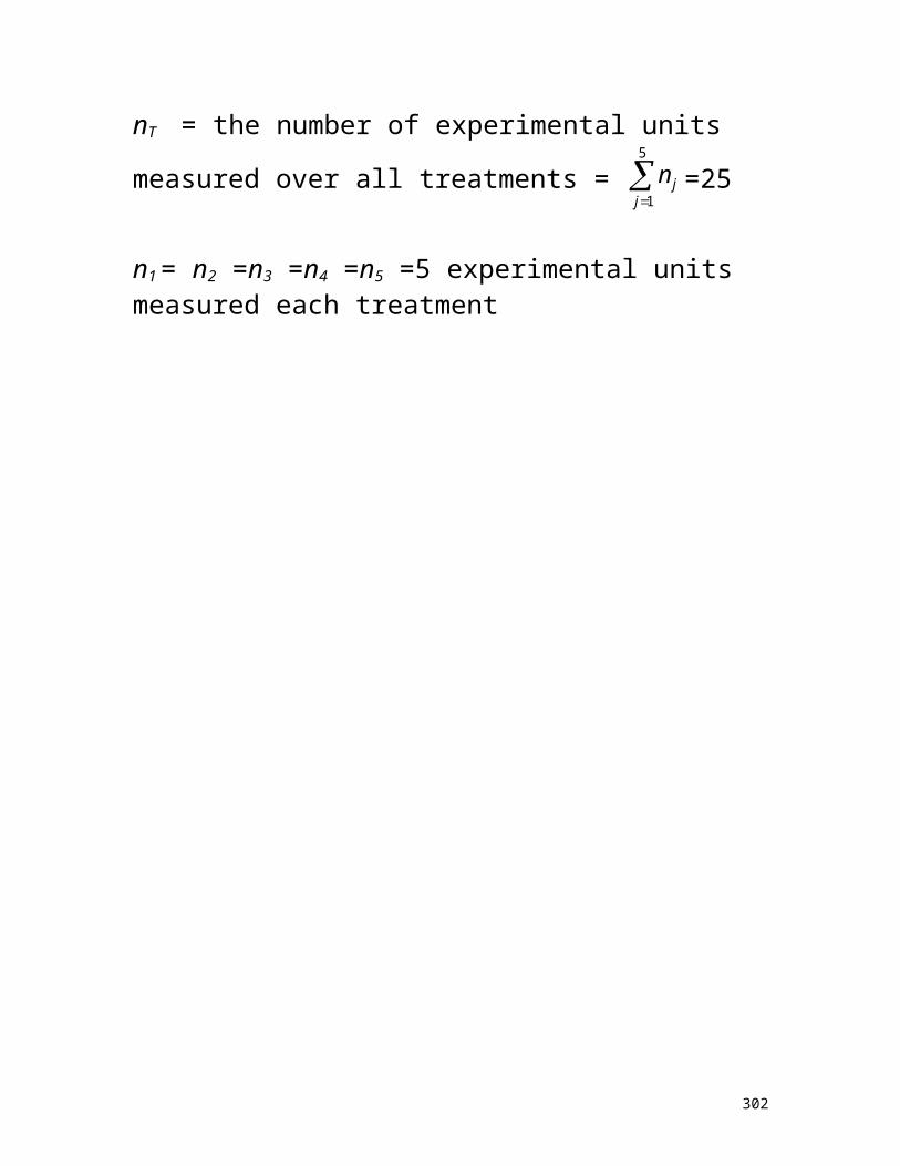
Fit Statistics
-2 Res Log Likelihood 166.7 AIC (smaller is better) 172.7 AICC (smaller is better) 173.3 BIC (smaller is better) 170.9
Type 3 Tests of Fixed Effects
Num Den Effect DF DF F Value Pr > F
A 2 6 222.03 <.0001
Least Squares Means
StandardEffect A Estimate Error DF t Value Pr>|t|A 1 16.2500 2.5709 6 6.32 0.0007A 2 23.3750 2.5709 6 9.09 <.0001A 3 28.7500 2.5709 6 11.18 <.0001
The SAS System 14
The Mixed Procedure
Differences of Least Squares Means
StandardEffect A A Estimate Error DF t Value Pr > |t|
A 1 2 -7.1250 0.5951 6 -11.97 <.0001A 1 3 -12.5000 0.5951 6 -21.00 <.0001A 2 3 -5.3750 0.5951 6 -9.03 0.0001
302
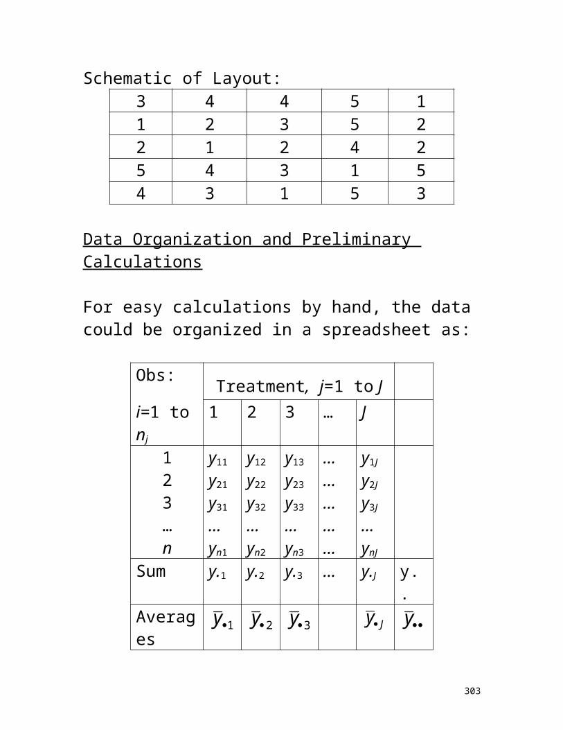
Randomized Complete Block (RCB)
With One Fixed-Effects Factor
REF: Neter et al., Ch 19, 20; Freese Handbook, page 34.
Introduction and Example
In RCB, treatments are assigned randomly, but only
within blocks of treatments
Restricting randomization of treatments to within blocks
(often called sites or trials) is used when the
experimental units can be grouped by another variable
that may impact the results
In field experiments with large experimental units,
blocking is often very useful in reducing error variance
with only a small reduction in error degrees of freedom
Blocks are most often random effects (we are interested
in the variance due to blocks)
The interest with RCB is with the factor, not with the
blocks; the blocks are simply used to reduce the
variability among experimental units
303

Example: Randomized Block Design (RCB), with Factor A
(six levels of fertilization: A1 to A6), and two sites.
Randomization of Factor A is restricted to within sites.
Site 1 Site 2
A1 = 9 A6=21 A4=25 A3=19
A3=15 A2=12 A1=12 A5=27
A5=20 A4=17 A2=16 A6=29
Response variable: biomass of grasses and herbs (kg)
2 observations per treatment – 1 in each site
304
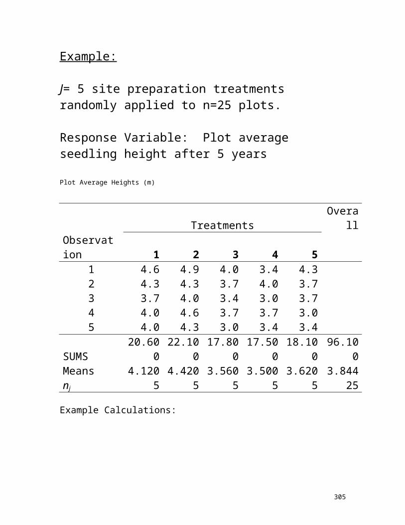
Organization of data for analysis using a statistics package:
Site Treatment yjk1 A1 91 A2 121 A3 151 A4 171 A5 201 A6 212 A1 122 A2 162 A3 192 A4 252 A5 272 A6 29
305

Main questions of interest:
Are the treatment means different?
Which means are different?
What are the estimated means and confidence
intervals for these estimates?
As for CRD with one factor
The organization of the data is the same for CRD with two
factors as with RCB, BUT the interpretation differs:
It is assumed that there is no interaction between the
blocks and the treatments. Not really appropriate to
check this since the randomization of treatments is
restricted to within blocks
Blocks are usually considered random-effects; want to
remove the effects of blocks from the analysis
Notation
306

Population:
jky = response variable measured on block j and treatment k
j=1 to J blocks; k=1 to K treatments
= the grand or overall mean regardless of treatment or block
Ak = the treatment effect for k
Bj = the block effect for block j
jk = is actually an interaction term between block and treatment, defined as:
)( BjkAjkjk y
307

For the experiment:
jkkABjjk eyy ˆˆ
y = the grand or overall mean of all measures from the experiment regardless of treatment; under the assumptions for the error terms, this will be an unbiased estimate of
jy = the mean of all measures from the experiment for a particular block j (includes all data for all levels of the treatment)
ky = the mean of all measures from the experiment for a particular treatment k over all blocks
BjAk ˆ,ˆ = under the error term assumptions, will be unbiased estimates of corresponding treatment effects for the population
jke = is defined as:
yyyy
yyyyyye
kjjk
kjjkjk )()()(
J= number of blocks and also the number of measures (experimental units) for treatment kKJ = total number of experimental units on which the response was measured
308

Sums of Squares:
SSESSSSSSy TRBLK
SSy: The sum of squared differences between the
observations and the grand mean:
1 1 1
2
JKdfyySSyK
k
J
jjk
SSTR : Sum of squared differences between the treatment
means, and the grand mean, weighted by the number of
blocks (experimental units in each treatment)
12
1
KdfyyJSSK
kkTR
SSBLK : Sum of squared differences between the block
means, and the grand mean, weighted by the number of
treatments (experimental units in each block)
11
2
JdfyyKSSJ
jjBLK
309

SSE: sum of squared differences between the observation
and the grand mean plus the treatment and block effects.
)1)(1( KJdfSSSSSSySSE BLKTR
Alternative computational formulae:
BLKTR
J
jjBLK
K
kkTR
K
k
J
jjk
SSSSSSySSEJKyyKSS
JKyyJSS
JKyySSy
2
1
22
1
2
2
1 1
2
310

Assumptions and Transformations:
Must meet assumptions for the error term to obtain
unbiased estimates of population means, and an unbiased
estimate of the variance of the error term
o independent observations (not time or space related)
o normality of the errors,
o equal variance for each treatment.
Use residual plot and a plot of the standardized errors
against the expected errors for a normal distribution to
check these assumptions.
To meet assumptions you might have to transform the y-
variable, as with other designs
311

Differences among treatment means
The main question is: Is there a difference between
treatment means:
H0: 1 = 2 = … = K
OR:
H0: (TR+ε) /ε = 1H1: (TR+ε)/ε > 1
Where ε is the variance of the error terms;
TR is fixed effect for the treatments.
312

Using an analysis of variance table:
Source df SS MS F p-valueBlock J-1 SSBLK MSA=
SSBLK /(J-1)
Treat. K-1 SSTR MSTR=SSTR /(K-1)
F= MSTR/MSE
Prob F> F(K-1),(dfE),1- α
Error (J-1)(K-1) SSE MSE=SSE/(J-1)(K-1)
Total JK -1 SSy
Source df MS E[MS]Block J-1 MSBLK 22
BLKK
Treat. K-1 MSTRTR
2
Error (J-1)(K-1)
MSE 2
Total nT -1
NOTE: Neter et al., assume blocks are fixed rather than random
is used here to represent fixed effects and 2
is used to represent
random effects.
313

From the ANOVA table:
MSEMS
KJSSEKSSF TRTR
)1)(1/(
)1/(
Under H0, this follows Fdf1,df2, 1- α where df1 is from the
numerator (K-1) and df2 is from the denominator (J-1)
(K-1)
If the F calculated is greater than the tabular F, or if the
p-value for F calculated is less than , reject H0, the
means of treatments in the population are likely not all
the same
314

Further analyses:
Can conduct multiple comparisons between means for the
K treatments:
using MSE and using J (number of blocks) as the
number of observations per treatment.
Can use t-tests of pairs of means -- must divide alpha by the
number of possible pairs
Confidence limits for treatment means
Treatment means:
JMSEty dfEk 21),(
As each block has a measure for each treatment.
315

SAS code and Results for the Example
PROC IMPORT OUT= WORK.biomass DATAFILE= "E:\frst430\lemay\examples\RCB_examples.xls" DBMS=EXCEL REPLACE; SHEET="'no reps$'"; GETNAMES=YES; MIXED=NO; SCANTEXT=YES; USEDATE=YES; SCANTIME=YES;RUN;
options ls=70 ps=50 pageno=1 nodate;
data biomass2; set biomass; lnbiomass=log(yjk);run;
PROC GLM data=biomass2;class site treatment;model lnbiomass=site treatment;random site;lsmeans treatment/pdiff tdiff;output out=glmout r=resid p=predict;run;
proc plot data=glmout;plot resid*predict='*';run;
proc univariate data=glmout normal plot;var resid;run;
316

The SAS System 1
The GLM Procedure
Class Level Information
Class Levels Values
Site 2 1 2
Treatment 6 A1 A2 A3 A4 A5 A6
Number of Observations Read 12 Number of Observations Used 12
317

The SAS System 2
The GLM Procedure
Dependent Variable: lnbiomass
Sum ofSource DF Squares Mean Square F Value
Model 6 1.38167231 0.23027872 189.72
Error 5 0.00606896 0.00121379
Corrected Total 11 1.38774127
Source Pr > F
Model <.0001
Error
Corrected Total
R-Square Coeff Var Root MSE lnbiomass Mean
0.995627 1.217186 0.034840 2.862299
318

Source DF Type I SS Mean Square F Value
Site 1 0.27612234 0.27612234 227.49Treatment 5 1.10554998 0.22111000 182.16
Source Pr > F
Site <.0001 Treatment <.0001
Source DF Type III SS Mean Square F Value
Site 1 0.27612234 0.27612234 227.49Treatment 5 1.10554998 0.22111000 182.16
Source Pr > F
Site <.0001 Treatment <.0001 The SAS System 3
The GLM Procedure
Source Type III Expected Mean Square
Site Var(Error) + 6 Var(Site)
Treatment Var(Error) + Q(Treatment)
319

The SAS System 4
The GLM Procedure Least Squares Means
lnbiomass LSMEAN Treatment LSMEAN Number
A1 2.34106561 1 A2 2.62874769 2 A3 2.82624459 3 A4 3.02604458 4 A5 3.14578457 5 A6 3.20590913 6
Least Squares Means for Effect Treatment t for H0: LSMean(i)=LSMean(j) / Pr > |t|
Dependent Variable: lnbiomass
i/j 1 2 3 4 5 6
1 -8.25735 -13.9261 -19.661 -23.0979 -24.8236 0.0004 <.0001 <.0001 <.0001 <.00012 8.257352 -5.66876 -11.4036 -14.8405 -16.5663 0.0004 0.0024 <.0001 <.0001 <.00013 13.92612 5.668763 -5.73487 -9.17177 -10.8975 <.0001 0.0024 0.0023 0.0003 0.00014 19.66098 11.40363 5.734869 -3.4369 -5.16266 <.0001 <.0001 0.0023 0.0185 0.00365 23.09789 14.84053 9.171771 3.436902 -1.72576 <.0001 <.0001 0.0003 0.0185 0.14506 24.82364 16.56629 10.89753 5.162661 1.725758 <.0001 <.0001 0.0001 0.0036 0.1450
NOTE: To ensure overall protection level, only probabilities associated with pre-planned comparisons should be used.
320

The SAS System 5
Plot of resid*predict. Symbol used is '*'.
resid ‚ ‚ 0.06 ˆ ‚ ‚ ‚ ‚ ‚ 0.04 ˆ * ‚ ‚ * ‚ ‚ ‚ 0.02 ˆ ‚ ‚ ‚ * ‚ * * ‚ 0.00 ˆ * * ‚ ‚ * * ‚ * ‚ ‚ -0.02 ˆ ‚ ‚ ‚ ‚ * ‚ -0.04 ˆ * ‚ ‚ ‚ ‚ ‚ -0.06 ˆ ‚ Š--ˆ-------ˆ-------ˆ-------ˆ-------ˆ-------ˆ-------ˆ-------ˆ-- 2.0 2.2 2.4 2.6 2.8 3.0 3.2 3.4
predict
321

The SAS System 6
The UNIVARIATE Procedure Variable: resid
Moments
N 12 Sum Weights 12Mean 0 Sum Observations 0Std Deviation 0.02348879 Variance 0.00055172Skewness 0 Kurtosis 0.25289374Uncorrected Corrected SS 0.00606896 SS 0.00606896Coeff Variation . Std Error Mean 0.00678063
Basic Statistical Measures
Location Variability
Mean 0.00000 Std Deviation 0.02349Median 0.00000 Variance 0.0005517Mode -0.00785 Range 0.08228Interquartile Range 0.01755
Tests for Location: Mu0=0
Test -Statistic- -----p Value------
Student's t t 0 Pr > |t| 1.0000Sign M 0 Pr >= |M| 1.0000Signed Rank S 2 Pr >= |S| 0.8979
322

Tests for Normality
Test --Statistic--- --p Value------
Shapiro-Wilk W 0.949629 Pr<W 0.6316Kolmogorov-Smirnov D 0.173219 Pr>D >0.1500Cramer-von Mises W-Sq 0.058634 Pr>W-Sq >0.2500Anderson-Darling A-Sq 0.344788 Pr>A-Sq >0.2500
Quantiles (Definition 5)
Quantile Estimate
100% Max 0.04114012 99% 0.04114012
The SAS System 7
The UNIVARIATE Procedure Variable: resid
Quantiles (Definition 5)
Quantile Estimate
95% 0.04114012 90% 0.03349673 75% Q3 0.00877283 50% Median 0.00000000 25% Q1 -0.00877283 10% -0.03349673 5% -0.04114012 1% -0.04114012 0% Min -0.04114012
323

Extreme Observations
-------Lowest------- -------Highest------
Value Obs Value Obs
-0.04114012 4 0.00785008 1-0.03349673 9 0.00785008 2-0.00969558 6 0.00969558 12-0.00785008 8 0.03349673 3-0.00785008 7 0.04114012 10
Stem Leaf # Boxplot 4 1 1 0 3 3 1 | 2 | 1 0 1 | 0 288 3 +--+--+ -0 882 3 +-----+ -1 0 1 | -2 | -3 3 1 | -4 1 1 0 ----+----+----+----+ Multiply Stem.Leaf by 10**-2
The SAS System 8
The UNIVARIATE Procedure Variable: resid Normal Probability Plot 0.045+ * ++++ | * +++++ | ++++ 0.015+ ++++ | +*+*+* * | * *+++* -0.015+ ++++ | ++++ | +++++ * -0.045+ ++++ * +----+----+----+----+----+----+----+----+----+----+ -2 -1 0 +1 +2
324

NOTE: Could use PROC MIXED instead of GLM (for interest only)* note: could use PROC MIXED instead of GLM for this;PROC IMPORT OUT= WORK.biomass DATAFILE= "E:\frst430\lemay\examples\RCB_examples.xls" DBMS=EXCEL REPLACE; SHEET="'no reps$'"; GETNAMES=YES; MIXED=NO; SCANTEXT=YES; USEDATE=YES; SCANTIME=YES;RUN;
options ls=70 ps=50 pageno=1 nodate;
data biomass2; set biomass; lnbiomass=log(yjk);run;
PROC MIXED data=biomass2;class site treatment;model lnbiomass=treatment;lsmeans treatment/pdiff;random site;run;
325

The SAS System 9
The Mixed Procedure
Model Information
Data Set WORK.BIOMASS2 Dependent Variable lnbiomass Covariance Structure Variance Components Estimation Method REML Residual Variance Method Profile Fixed Effects SE Method Model-Based Degrees of Freedom Method Containment
Class Level Information
Class Levels Values
Site 2 1 2 Treatment 6 A1 A2 A3 A4 A5 A6
Dimensions Covariance Parameters 2 Columns in X 7 Columns in Z 2 Subjects 1 Max Obs Per Subject 12
Number of Observations Number of Observations Read 12 Number of Observations Used 12 Number of Observations Not Used 0
Iteration HistoryIteration Evaluations -2 Res Log Like Criterion 0 1 2.84456806 1 1 -13.67079866 0.00000000 Convergence criteria met.
326

The SAS System 10
The Mixed Procedure
Covariance Parameter Estimates
Cov Parm Estimate
Site 0.04582 Residual 0.001214
Fit Statistics
-2 Res Log Likelihood -13.7AIC (smaller is better) -9.7AICC (smaller is better) -5.7BIC (smaller is better) -12.3
Type 3 Tests of Fixed Effects
Num DenEffect DF DF F Value Pr > F
Treatment 5 5 182.16 <.0001
Least Squares Means
StandardEffect Treat Estimate Error DF t Value Pr>|t|
Treatment A1 2.3411 0.1533 5 15.27 <.0001Treatment A2 2.6287 0.1533 5 17.14 <.0001Treatment A3 2.8262 0.1533 5 18.43 <.0001Treatment A4 3.0260 0.1533 5 19.73 <.0001Treatment A5 3.1458 0.1533 5 20.51 <.0001Treatment A6 3.2059 0.1533 5 20.91 <.0001
327

Differences of Least Squares Means
StandardEffect Treat Treat Estimate Error DF t Value
Treatment A1 A2 -0.2877 0.03484 5 -8.26Treatment A1 A3 -0.4852 0.03484 5 -13.93Treatment A1 A4 -0.6850 0.03484 5 -19.66Treatment A1 A5 -0.8047 0.03484 5 -23.10Treatment A1 A6 -0.8648 0.03484 5 -24.82Treatment A2 A3 -0.1975 0.03484 5 -5.67Treatment A2 A4 -0.3973 0.03484 5 -11.40Treatment A2 A5 -0.5170 0.03484 5 -14.84Treatment A2 A6 -0.5772 0.03484 5 -16.57Treatment A3 A4 -0.1998 0.03484 5 -5.73Treatment A3 A5 -0.3195 0.03484 5 -9.17Treatment A3 A6 -0.3797 0.03484 5 -10.90Treatment A4 A5 -0.1197 0.03484 5 -3.44Treatment A4 A6 -0.1799 0.03484 5 -5.16Treatment A5 A6 -0.06012 0.03484 5 -1.73
Differences of Least Squares Means
Effect Treatment Treatment Pr > |t|Treatment A1 A2 0.0004Treatment A1 A3 <.0001Treatment A1 A4 <.0001Treatment A1 A5 <.0001Treatment A1 A6 <.0001Treatment A2 A3 0.0024Treatment A2 A4 <.0001Treatment A2 A5 <.0001Treatment A2 A6 <.0001Treatment A3 A4 0.0023Treatment A3 A5 0.0003Treatment A3 A6 0.0001Treatment A4 A5 0.0185Treatment A4 A6 0.0036
328

Treatment A5 A6 0.1450Randomized Block Design with other experiments
RCB with Two Fixed Factors
Within each block. treatments are randomly located to
each experimental unit, but each treatment is a
combination of two factors
Example: Randomized Block Design (RCB), with three
types of food (Factor A: A1 to A3), two species of fish
(Factor B) and two labs (blocks). Randomization of
treatments (e.g., A1, B2) is restricted to within labs.
Lab 1 Lab 2
A1B1 = 6 A1B2=5 A3B1=1
1
A3B2=1
2
A3B1=10 A2B2=8 A1B1=4 A2B2=9
329

A2B1=7 A3B2=1
2
A2B1=8 A1B2=5
Response variable: weight gain of fish (kg)
Experimental unit: one tank of fish; 6 tanks in each lab
Organization of data for analysis using a statistics package:
SiteA
FoodB
Species yijk1 A1 B1 61 A1 B2 51 A2 B1 81 A2 B2 71 A3 B1 101 A3 B2 122 A1 B1 42 A1 B2 52 A2 B1 92 A2 B2 82 A3 B1 112 A3 B2 12
Main questions of interest—same as for RCB:
Is there an interaction between factors? If not, is there
a difference between means for Factor A? Factor B?
330

Which means are different? What are the estimated
means and confidence intervals for these estimates?
We are not really interested in the blocks – just used to
reduce the amount of variation
Models The model is a mixture between a single factor RCB and a 2-factor CRD; interpretation is more difficult
o Blocks are usually random not fixed factorso Blocks are used to reduce variability within
treatments; not of interest on their own
Population:
jkly = response variable measured on block j and treatment kl
j=1 to J blocks; k=1 to K levels for Factor A; l=1 to L levels for Factor B
Definition of terms follows other designs
331

Test for Interactions and Main Effects
H0: No interaction between Factor A and Factor B
H1: InteractionOR:
H0: (A XB+ε)/ε = 1H1: (A X B+ε)/ε > 1
Where ε is the variance of the error terms;
A X B is the interaction between Factor A and Factor B
fixed-effect treatments
332

ANOVA: Blocks Random, Factor A and Factor B are Fixed
Source df SS MS F ??? correct? BLK. J-1 SSBLK MSBLK=
SSBLK/(J-1)F= MSBLK/MSE
Factor A
K-1 SSA MSA=SSA/(K-1)
F= MSA/MSBXT
Factor B
L-1 SSB MSB=SSB/(L-1)
F= MSB/MSBXT
A X B (K-1)(L-1) SSAXB MSAXB=SSAXB /(K-1)(L-1)
F= MSAB/MSE
Error (J-1)(KL-1)
SSE MSE= SSE/(J-1)(KL-1)
Total nT -1 SSy
Source
df MS p-value E[MS]
BLK. J-1 MSBLK Prob F> F(J-1),(dfE), 1- α
22BLKKL
A K-1 MSA Prob F> F(K-1),(dfBXT),1- α
A 2
B L-1 MSB Prob F> F(L-1),(dfBXT),1- α
B 2
AXB (J-1)(L-1) MSAXB Prob F> F dfAXB,dfE,,1- α
BA
2
Error (J-1)(KL-1) MSE 2
Total nT -1
is used here to represent fixed effects.
333
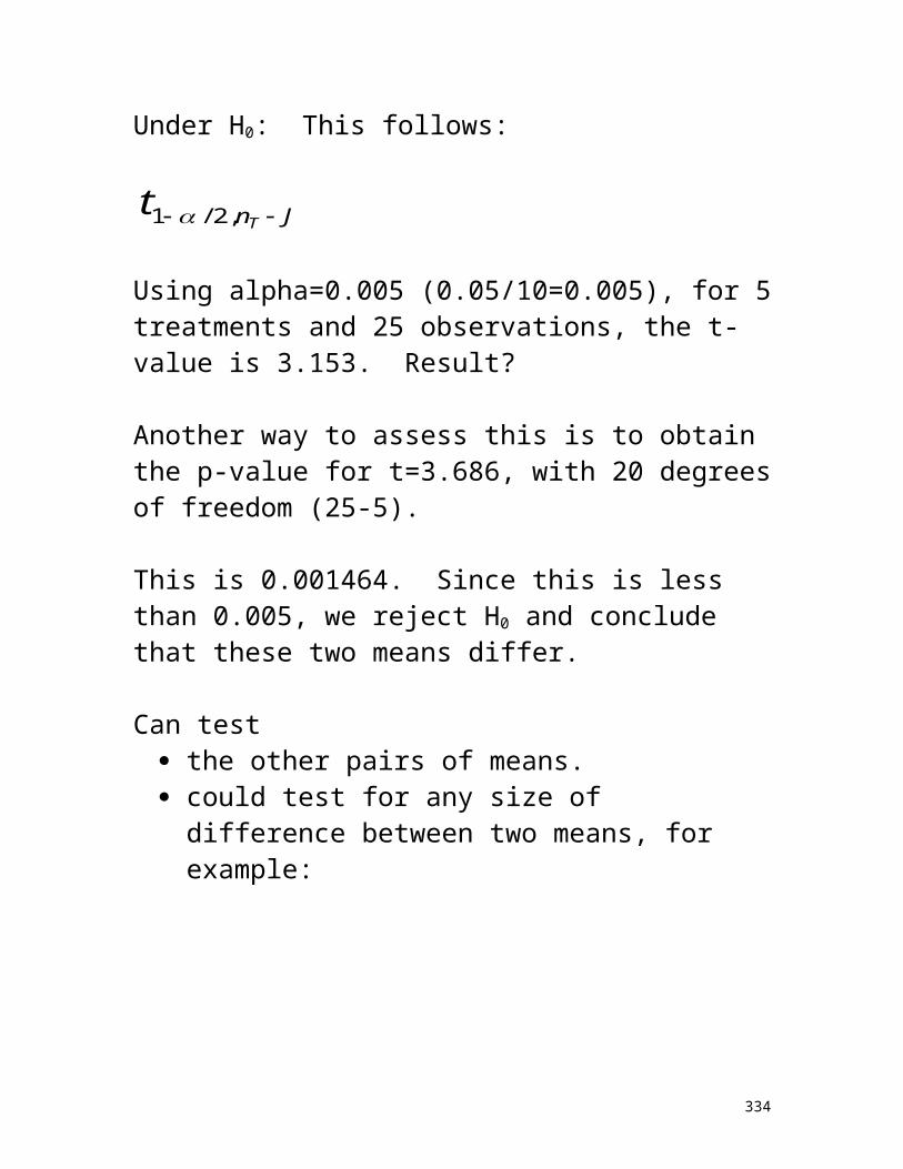
SAS code for example and output: Food and Species Fixed effects; Site is a Random Effect.
PROC IMPORT OUT= WORK.blocktwo DATAFILE= "E:\frst430\lemay\examples\RCB_examples.xls" DBMS=EXCEL REPLACE; SHEET="'2-factors$'"; GETNAMES=YES; MIXED=NO; SCANTEXT=YES; USEDATE=YES; SCANTIME=YES;RUN;options ls=70 ps=50 pageno=1 nodate;data blocktwo2; set blocktwo;lnfishwt=log(yijk);run;
PROC GLM data=blocktwo2;class site food species;model lnfishwt=site food species food*species;random site;lsmeans food/pdiff tdiff;lsmeans species/pdiff tdiff;lsmeans food*species/pdiff tdiff;output out=glmout r=resid p=predict;run;
proc plot data=glmout;plot resid*predict='*';run;proc univariate data=glmout normal plot;var resid;run;
334

The SAS System 1
The GLM Procedure
Class Level Information
Class Levels Values
Site 2 1 2 Food 3 A1 A2 A3 Species 2 B1 B2
Number of Observations Read 12 Number of Observations Used 12 The SAS System 2 The GLM Procedure
Dependent Variable: lnfishwt
Sum ofSource DF Squares Mean Square F Value
Model 6 1.38600089 0.23100015 11.29Error 5 0.10230621 0.02046124Corrected Total 11 1.48830710
Source Pr > F
Model 0.0088 Error Corrected Total
R-Square Coeff Var Root MSE lnfishwt Mean
0.931260 7.043771 0.143043 2.030770
335

Source DF Type I SS Mean Square FValueSite 1 0.00028852 0.00028852 0.01Food 2 1.35137097 0.67568548 33.02Species 1 0.00028852 0.00028852 0.01Food*Species 2 0.03405288 0.01702644 0.83
Source Pr > F Site 0.9101 Food 0.0013 Species 0.9101 Food*Species 0.4876
Source DF Type III SS Mean Square F ValueSite 1 0.00028852 0.00028852 0.01Food 2 1.35137097 0.67568548 33.02Species 1 0.00028852 0.00028852 0.01Food*Species 2 0.03405288 0.01702644 0.83 Source Pr > F Site 0.9101 Food 0.0013 Species 0.9101 Food*Species 0.4876
The SAS System 4
The GLM Procedure
Source Type III Expected Mean SquareSite Var(Error) + 6 Var(Site)Food Var(Error) + Q(Food,Food*Species)Species Var(Error) + Q(Species,Food*Species)Food*Species Var(Error) + Q(Food*Species)
336

The SAS System 5
The GLM Procedure Least Squares Means
lnfishwt LSMEAN Food LSMEAN Number A1 1.59923241 1 A2 2.07550445 2 A3 2.41757342 3
Least Squares Means for Effect Food t for H0: LSMean(i)=LSMean(j) / Pr > |t|
Dependent Variable: lnfishwt
i/j 1 2 3 1 -4.70873 -8.09065 0.0053 0.0005 2 4.708733 -3.38191 0.0053 0.0196 3 8.090648 3.381915 0.0005 0.0196NOTE: To ensure overall protection level, only probabilities associated with pre-planned comparisons should be used. The SAS System 6
The GLM Procedure Least Squares Means lnfishwt H0:LSMean1=LSMean2Species LSMEAN t Value Pr > |t|
B1 2.02586672 -0.12 0.9101 B2 2.03567347
337

The SAS System 7
The GLM Procedure Least Squares Means
lnfishwt LSMEANFood Species LSMEAN Number
A1 B1 1.58902692 1 A1 B2 1.60943791 2 A2 B1 2.13833306 3 A2 B2 2.01267585 4 A3 B1 2.35024018 5 A3 B2 2.48490665 6
Least Squares Means for Effect Food*Speciest for H0: LSMean(i)=LSMean(j) / Pr > |t|
Dependent Variable: lnfishwt
i/j 1 2 3 4 5 6
1 -0.14269 -3.84015 -2.96169 -5.32158 -6.26302 0.8921 0.0121 0.0315 0.0031 0.0015
2 0.142692 -3.69746 -2.819 -5.17889 -6.12033 0.8921 0.0140 0.0372 0.0035 0.0017
3 3.840152 3.697461 0.878459 -1.48142 -2.42287 0.0121 0.0140 0.4199 0.1986 0.0599
4 2.961693 2.819002 -0.87846 -2.35988 -3.30133 0.0315 0.0372 0.4199 0.0648 0.0214
5 5.321577 5.178885 1.481425 2.359883 -0.94144 0.0031 0.0035 0.1986 0.0648 0.3897
6 6.263019 6.120327 2.422866 3.301325 0.941442 0.0015 0.0017 0.0599 0.0214 0.3897
NOTE: To ensure overall protection level, only probabilities associated with pre-planned comparisons should be used.
338

The SAS System 8
Plot of resid*predict. Symbol used is '*'.
resid ‚ ‚ 0.2 ˆ * ‚ ‚ ‚ ‚ ‚ ‚ 0.1 ˆ ‚ ‚ * ‚ * * ‚ ‚ ‚ 0.0 ˆ ** * ‚ ‚ ‚ ‚ * * ‚ * ‚ -0.1 ˆ ‚ ‚ ‚ ‚ ‚ ‚ -0.2 ˆ * ‚ Š-ˆ---------ˆ---------ˆ---------ˆ---------ˆ---------ˆ---------ˆ- 1.4 1.6 1.8 2.0 2.2 2.4 2.6
predict
NOTE: 1 obs hidden.
339

The SAS System 9
The UNIVARIATE Procedure Variable: resid
Moments
N 12 Sum Weights 12Mean 0 Sum Observations 0Std Deviation 0.096439 Variance 0.00930056Skewness 0 Kurtosis 1.73130021Uncorrected SS 0.10230621 Corrected SS 0.10230621Coeff Variation . Std Error Mean 0.02783967
(some outputs on basic stats for residuals trimmed off) Tests for Normality
Test --Statistic--- -----p Value---
Shapiro-Wilk W 0.95208 Pr < W 0.6676 Kolmogorov-Smirnov D 0.146392 Pr > D >0.1500Cramer-von Mises W-Sq 0.056429 Pr>W-Sq >0.2500Anderson-Darling A-Sq 0.357776 Pr>A-Sq >0.2500
Quantiles (Definition 5) Quantile Estimate 100% Max 0.1978292 99% 0.1978292 95% 0.1978292 90% 0.0716691 75% Q3 0.0581767 50% Median 0.0000000 25% Q1 -0.0581767 10% -0.0716691 5% -0.1978292 1% -0.1978292 0% Min -0.1978292
340

Extreme Observations
------Lowest------- -------Highest------
Value Obs Value Obs
-0.19782918 7 0.00490338 12-0.07166907 4 0.05255846 11-0.06379489 3 0.06379489 9-0.05255846 5 0.07166907 10-0.00490338 6 0.19782918 1
Stem Leaf # Boxplot 2 0 1 | 1 | 1 | 0 567 3 +-----+ 0 00 2 *--+--* -0 00 2 | | -0 765 3 +-----+ -1 | -1 | -2 0 1 | ----+----+----+----+ Multiply Stem.Leaf by 10**-1
The UNIVARIATE Procedure Variable: resid
Normal Probability Plot 0.225+ +++++ | *++++ | +++++ 0.075+ *++*++* | +*+*++ | ++*+* -0.075+ *++*++* | +++++ | ++++* -0.225++++++ +----+----+----+----+----+----+----+----+----+----+ -2 -1 0 +1 +2
341

RCB with One fixed, one random factor Within each block treatments are randomly located to
each experimental unit, but each treatment is a
combination of two factors
For one factor, we are interested in comparing treatment
means
For the other factor, we are interested in obtaining an
estimate of the variance of the response variable that is
due to that factor
Example: Randomized Block Design (RCB), with three
types of fertilizer (Factor A: A1 to A3), two genetic
families of pine trees (Factor B) and two sites (blocks).
Randomization of treatments (e.g., A1, B2) is
restricted to within sites.
Blocks are random; factor B is random (random
selection of possible families)
342

Interpretation will differ from RCB with two factors;
F-tests will vary also, as Expected Mean Squares will
be different
If there is no interaction among the two factors, we
can interpret the factors separately
For Factor A: use multiple comparisons to compare
factor level means
For Factor B: obtain an estimate of the variance due
to this factor.
NOTE: we could use least squares analysis of
variance for this analysis. HOWEVER: using
MIXED models with Maximum Likelihood is
considered a better approach for mixed-effects (one
random, one fixed effects factor)
343

Incomplete Block Design
Like RCB, BUT there are not enough experimental units in each block to have every treatment in each block – incomplete
For example:
We have 2 sites. There are 4 experimental units in each site. However, we have 5 treatments! There are not enough experimental units in site 1 to have all 5 treatments, nor is there enough experimental units in site 2 to have all 5. (REF: Chapter 28 of textbook)
344

RCB with replicates in each block Within each block there are several replicates of each
treatment
Sometimes called “Generalized RCB”
Example: Randomized Block Design (RCB), with Factor A
(three types of food: A1 to A3), and two labs (blocks).
Randomization of Factor A is restricted to within labs.
Lab 1 Lab 2
A1 = 6 A1=5 A3=11 A3=12
A3=10 A2=8 A1=4 A2=9
A2=7 A3=12 A2=8 A1=5
Response variable: weight gain of fish (kg)
Experimental unit: one tank of fish; 6 tanks in each lab
Organization of data for analysis using a statistics package:
Site Treatment Replicate yijk
345

1 A1 1 61 A1 2 51 A2 1 81 A2 2 71 A3 1 101 A3 2 122 A1 1 42 A1 2 52 A2 1 92 A2 2 82 A3 1 112 A3 2 12
Main questions of interest—same as for RCB:
Are the treatment means different? Which means are
different? What are the estimated means and
confidence intervals for these estimates?
346

Models
Population:
ijky = response variable measured on experimental unit I in block j and treatment k
j=1 to J blocks; k=1 to K treatments; i=1 to n replicates
= the grand or overall mean regardless of treatment or block
jBLK = the block effect for j
TRk = the treatment effect for block k
jkTRBLK = the interaction effect between block j and treatment k
ijk = is error term, specific to observation i
347

For the experiment:
ijkjkTRBLKkTRjBLKijk eyy ˆˆˆ
y = the grand or overall mean of all measures from the experiment regardless of treatment or block; under the assumptions for the error terms, this will be an unbiased estimate of
jky = the mean of all measures from the experiment for a particular block j and experiment k
jy = the mean of all measures from the experiment for a particular block j (includes all data for all levels of the treatments)
ky = the mean of all measures from the experiment for a particular level k of the Factor A (includes all data for all blocks)
jkTRBLKkTRjBLK ˆ,ˆ,ˆ = under the error term assumptions, will be unbiased estimates of corresponding treatment, block, and block by treatment for the population
ijke = the difference between a particular measure for an experimental unit i, and the mean for the block j and treatment k that was applied to it
jkijkijk yye njk = the number of experimental units measured in the block j and treatment knT = the number of experimental units measured over all
blocks and treatments =
K
k
J
jjkn
1 1
348

Sums of Squares:
SSESSSSSSSSy BLKTRTRBLK
SSy: The sum of squared differences between the
observations and the grand mean:
1 1 1 1
2
T
K
k
J
j
n
iijk ndfyySSy
jk
SSBLK: Sum of squared differences between the block
means and the grand mean, weighted by the number of
experimental units for each block:
11 1
2
JdfyynSSK
k
J
jjjkBLK
SSTR: Sum of squared differences between the level means
for factor A and the grand mean, weighted by the number
of experimental units for each treatment:
11 1
2
KdfyynSSK
k
J
jkjkTR
349

SSBLK X TR: Sum of squared differences between means for
block j and treatment k and the grand mean, minus the
block and treatment level differences, all weighted by the
number of experimental units for each block and treatment:
K
k
J
jjkjkjk
TRBLK
yyyyyyn
SS
1 1
2))()()((
Since some of the terms cancel out we obtain:
)(1 1
2
K
k
J
jjkjkjkTRBLK yyyynSS
SSE: Sum of squared differences between the observed
values for each experimental unit and the treatment means:
K
k
J
jT
n
ijkijk JKndfyySSE
jk
1 1 1
2
350

Assumptions regarding the error term
Must meet assumptions to obtain unbiased estimates of
population means, and an unbiased estimate of the
variance of the error term as with other designs
Process: do your analysis with the measured response variable Check the residual plot and normal plot to see if
assumptions are met if assumptions of the error term are not met, transform
the y-variable do the analysis again and check the assumptions; if not
me, try another transformation may have to switch to another method: generalized
linear models, etc.
351

Test for Interactions and Main Effects
Although an interaction between treatments and blocks would result in a difficult interpretation of results, this can be tested first.
H0: No interactionH1: Interaction
OR:
H0: (B X T+ε)/ε = 1
H1: (B X T+ε)/ε > 1
Where ε is the variance of the error terms;
BXT is the interaction between blocks and fixed
treatments; since blocks are random, the interaction
between blocks and treatments is also random.
352
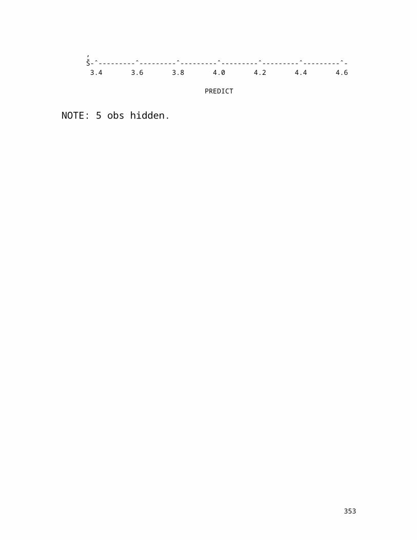
Using an analysis of variance table: Blocks Random, Treatments Fixed
Source df SS MS F BLK. J-1 SSBLK MSBLK=
SSBLK/(J-1)F= MSBLK/MSE
TR. K-1 SSTR MSTR=SSTR/(K-1)
F= MSTR/MSBXT
BLKX TR
(J-1)(K-1) SSBXT MSBXT=SSBXT /
(J-1)(K-1)
F= MSBT/MSE
Error nT -JK SSE MSE= SSE/(nT -JK)
Total nT -1 SSy
Source
df MS
p-value E[MS]
BLK. J-1 MSBLK Prob F> F(J-1),(dfE), 1- α
22BLKKn
TR. K-1 MSTR Prob F> F(K-1),(dfBXT),1- α
TRTBn 22
BLKX TR
(J-1)(K-1)
MSBXT Prob F> F dfBXT,dfE,,1- α
TBn 22
Error nT -JK MSE 2
Total nT -1 is used here to represent fixed effects.Assuming all n are equal (same number of replicates in each block and treatment combination)For the interactions:
353

MSEMS
JKnSSEKJSSF TB
T
TB
)/(
)1)(1/(
Under H0, this follows Fdf1,df2, 1- α where df1 is from the
numerator (J-1)(K-1), and df2 is from the denominator
(nT-JK)
If the F calculated is greater than the tabular F, or if the
p-value for F calculated is less than , reject H0.
o The means of Factor A are influenced by the levels
of the blocks; the design should have been a
completely randomized design for ease of
interpretation
o Graph the means of all treatments by block and try
to interpret results
354

If there are no interactions (hopefully the case) we can
look at the impact of the treatments
Factor A:
H0: 1 = 2 = … = J
OR:
H0: (A+nB X Tε) /(n
B X Tε ) = 1H1: (A+n
B X Tε) /(nB X T ε ) > 1
Where ε is the variance of the error terms; B X
T is the variance for the interaction between
blocks and treatments; A is fixed effect for Factor A.
355

From the ANOVA table:
TB
TR
TB
TR
MSMS
KJSSKSSF
)1)(1/(
)1/(
Under H0, this follows Fdf1,df2, 1- α where df1 is from the
numerator (K-1) and df2 is from the denominator
(J-1)(K-1)
If the F calculated is greater than the tabular F, or if the
p-value for F calculated is less than , reject H0.
o The true means of the treatment in the population
are likely not all the same
o Graph the means of treatment levels
o Conduct multiple comparisons between means for
the K levels of the treatment
356
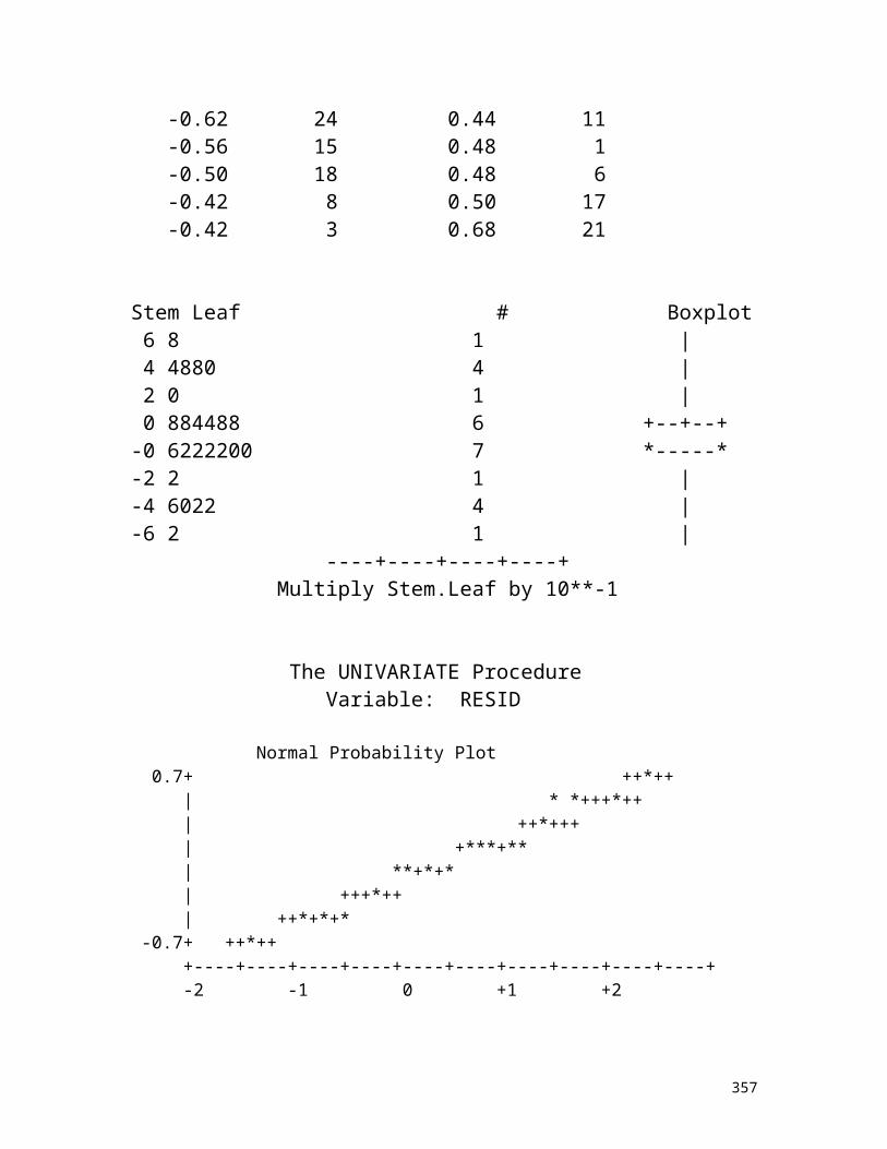
SAS code and Results for example:
PROC IMPORT OUT= WORK.fishweight DATAFILE= "E:\frst430\lemay\examples\RCB_examples.xls" DBMS=EXCEL REPLACE; SHEET="'reps$'"; GETNAMES=YES; MIXED=NO; SCANTEXT=YES; USEDATE=YES; SCANTIME=YES;RUN;options ls=70 ps=50 pageno=1 nodate;data fishweight2; set fishweight;lnfishwt=log(yijk);run;
PROC GLM data=fishweight2;class site treatment;model lnfishwt=site treatment site*treatment;random site site*treatment;test h=treatment e=site*treatment;lsmeans treatment/e=site*treatment pdiff tdiff;output out=glmout r=resid p=predict;run;proc plot data=glmout;plot resid*predict='*';run;proc univariate data=glmout normal plot;var resid;run;
* note: could use PROC MIXED instead of GLM for this – for interest only;PROC MIXED data=fishweight2;class site treatment;model lnfishwt=treatment;lsmeans treatment/pdiff;random site site*treatment;run;
357

The SAS System 1 The GLM Procedure
Class Level Information
Class Levels Values
Site 2 1 2 Treatment 3 A1 A2 A3
Number of Observations Read 12 Number of Observations Used 12
The SAS System 2 The GLM Procedure
Dependent Variable: lnfishwt
Sum ofSource DF Squares Mean Square F Value
Model 5 1.41053220 0.28210644 21.76
Error 6 0.07777490 0.01296248
Corrected Total 11 1.48830710
Source Pr > F
Model 0.0009
Error
Corrected Total
R-Square Coeff Var Root MSE lnfishwt Mean0.947743 5.606391 0.113853 2.030770
358

Source DF Type I SS Mean Square F Value
Site 1 0.00028852 0.00028852 0.02Treatment 2 1.35137097 0.67568548 52.13Site*Treatment 2 0.05887271 0.02943636 2.27
Source Pr > F
Site 0.8863 Treatment 0.0002 Site*Treatment 0.1844
Source DF Type III SS Mean Square F Value
Site 1 0.00028852 0.00028852 0.02Treatment 2 1.35137097 0.67568548 52.13Site*Treatment 2 0.05887271 0.02943636 2.27
Source Pr > F
Site 0.8863 Treatment 0.0002 Site*Treatment 0.1844 The SAS System 4
The GLM Procedure
Source Type III Expected Mean Square
Site Var(Error) + 2 Var(Site*Treatment) + 6 Var(Site)
Treatment Var(Error) + 2 Var(Site*Treatment) +Q(Treatment)
Site*Treatment Var(Error) + 2 Var(Site*Treatment)
359

The SAS System 5
The GLM Procedure Least Squares MeansStandard Errors and Probabilities Calculated Using the Type III MS for Site*Treatment as an Error Term
lnfishwt LSMEANS
Treatment LSMEAN Number
A1 1.59923241 1A2 2.07550445 2A3 2.41757342 3
Least Squares Means for Effect Treatment t for H0: LSMean(i)=LSMean(j) / Pr > |t|
Dependent Variable: lnfishwt
i/j 1 2 3
1 -3.9258 -6.74539 0.0592 0.0213 2 3.925799 -2.81959 0.0592 0.1061 3 6.745393 2.819594 0.0213 0.1061
NOTE: To ensure overall protection level, only probabilities associated with pre-planned comparisons should be used.
360

The SAS System 6 The GLM Procedure
Dependent Variable: lnfishwtTests of Hypotheses Using the Type IIIMS for Site*Treatment as an Error Term
Source DF Type III SS Mean Square F ValueTreatment 2 1.35137097 0.67568548 22.95
Source Pr > F Treatment 0.0417 The SAS System 7 Plot of resid*predict. Symbol used is '*'.resid ‚ ‚ 0.15 ˆ ‚ ‚ ‚ ‚ ‚ * 0.10 ˆ ‚ * * ‚ ‚ ‚ * ‚ * 0.05 ˆ ‚ * ‚ ‚ ‚ ‚ 0.00 ˆ ‚ ‚ ‚ ‚ ‚ *-0.05 ˆ ‚ * ‚ * ‚ ‚ ‚ * *-0.10 ˆ ‚ * ‚ ‚ ‚ ‚-0.15 ˆ ‚ Š-ˆ---------ˆ---------ˆ---------ˆ---------ˆ---------ˆ---------ˆ- 1.4 1.6 1.8 2.0 2.2 2.4 2.6
predict
361

The SAS System 8
The UNIVARIATE Procedure Variable: resid
Moments
N 12 Sum Weights 12Mean 0 Sum Observations 0Std Deviation 0.08408594 Variance 0.00707045Skewness 0 Kurtosis -1.9620284Uncorrected SS 0.0777749 Corrected SS 0.0777749Coeff Variation . Std Error Mean 0.02427352
Basic Statistical Measures
Location Variability
Mean 0 Std Deviation 0.08409Median 2.22E-16 Variance 0.00707Mode . Range 0.22314Interquartile Range 0.15793
Tests for Location: Mu0=0
Test -Statistic- -----p Value------
Student's t t 0 Pr > |t| 1.0000Sign M 0 Pr >= |M| 1.0000Signed Rank S 0 Pr >= |S| 1.0000
362

Tests for NormalityTest --Statistic--- ---p Value----
Shapiro-Wilk W 0.871142 Pr<W 0.0676Kolmogorov-Smirnov D 0.19756 Pr>D >0.1500Cramer-von Mises W-Sq 0.1182 Pr>W-Sq 0.0563Anderson-Darling A-Sq 0.672686 Pr>A-Sq 0.0611
Quantiles (Definition 5)
Quantile Estimate 100% Max 0.1115718 99% 0.1115718
The SAS System 9
The UNIVARIATE Procedure Variable: resid
Quantiles (Definition 5)
Quantile Estimate
95% 0.1115718 90% 0.0911608 75% Q3 0.0789632 50% Median 0.0000000 25% Q1 -0.0789632 10% -0.0911608 5% -0.1115718 1% -0.1115718 0% Min -0.1115718
363

Extreme Observations
-------Lowest------ ------Highest------
Value Obs Value Obs
-0.1115718 7 0.0588915 9 -0.0911608 2 0.0667657 3 -0.0911608 5 0.0911608 1 -0.0667657 4 0.0911608 6 -0.0588915 10 0.1115718 8
Stem Leaf # Boxplot 1 1 1 | 0 6799 4 +-----+ 0 4 1 *--+--* -0 4 1 | | -0 9976 4 +-----+ -1 1 1 | ----+----+----+----+ Multiply Stem.Leaf by 10**-1
The SAS System 10
The UNIVARIATE Procedure Variable: resid
Normal Probability Plot 0.125+ ++++*+ | * *++*++* | +*++++ | ++++* | *++*++* * -0.125+ +*++++ +----+----+----+----+----+----+----+----+----+----+ -2 -1 0 +1 +2
364

OPTIONAL – FOR INTEREST ONLY The SAS System 11
The Mixed Procedure
Model Information
Data Set WORK.FISHWEIGHT2Dependent Variable lnfishwtCovariance Structure Variance ComponentsEstimation Method REMLResidual Variance Method ProfileFixed Effects SE Method Model-BasedDegrees of Freedom Method Containment
Class Level Information
Class Levels Values
Site 2 1 2 Treatment 3 A1 A2 A3
Dimensions
Covariance Parameters 3 Columns in X 4 Columns in Z 8 Subjects 1 Max Obs Per Subject 12
Number of Observations
Number of Observations Read 12 Number of Observations Used 12 Number of Observations Not Used 0
365

Iteration History
Iteration Evaluations -2Res LogLike Criterion
0 1 -7.96941039 1 3 -8.14751521 0.00045738 2 2 -8.15260197 0.00000806 3 1 -8.15270255 0.00000000 The SAS System 12
The Mixed Procedure
Convergence criteria met.
Covariance Parameter Estimates Cov Parm Estimate
Site 0 Site*Treatment 0.003378 Residual 0.01296
Fit Statistics
-2 Res Log Likelihood -8.2 AIC (smaller is better) -4.2 AICC (smaller is better) -2.2 BIC (smaller is better) -6.8
366

Type 3 Tests of Fixed Effects
Num DenEffect DF DF F Value Pr > F
Treatment 2 2 34.27 0.0284
Least Squares Means
StandardTreatment Estimate Error DF t Value Pr > |t|
Treatment A1 1.5992 0.07021 2 22.78 0.0019Treatment A2 2.0755 0.07021 2 29.56 0.0011Treatment A3 2.4176 0.07021 2 34.43 0.0008
Differences of Least Squares Means
StandardEffect Treatments Estimate Error DF t Value
Treatment A1 A2 -0.4763 0.09929 2 -4.80Treatment A1 A3 -0.8183 0.09929 2 -8.24Treatment A2 A3 -0.3421 0.09929 2 -3.45
Differences of Least Squares Means
Effect Treatments Pr > |t|
Treatment A1 A2 0.0408Treatment A1 A3 0.0144Treatment A2 A3 0.0749
367

Latin Square (LS) With One Fixed-Effects Factor
REF: Neter et al., Chapter 26 (White-newest edition) or
Chapter 28 (Blue – older edition in the library)
Introduction and Example
In RCB, treatments are assigned randomly, but only
within blocks of treatments; blocking is in “one”
direction
The Latin Square Design extends grouping of
experimental units to two variables. For example,
two sites may represent north versus south facing
stands, and there might be a moisture gradient within
sites
Treatments are randomly assigned in two directions;
treatment appears once in every row and every column
368

Example:
Response variable: average 5-year height growth in each
experimental unit (plot) in cm
Treatments: four different species, A1 to A4
Nutrient Gradient from East to West; Moisture Gradient
from North to South
Means
A2=40 A1=35 A4=53 A3=47 43.75A4=48 A3=46 A2=39 A1=34 41.75A1=27 A4=53 A3=45 A2=41 41.50A3=44 A2=39 A1=31 A4=52 41.50
Means 39.75 43.25 42.00 43.50 42.125
Treatment Means:
A1: 31.75 A2: 39.75 A3: 45.50 A4: 51.50
16 experimental units
369

Comparison of Degrees of Freedom for CRD, RCB, LS for 16 experimental units, 4 treatments, J=K=L=4 blocks (rows/columns)
Source CRD Source RCB Source LSTreatment 3 Treatment 3 Treatment 3
Block 3 Row 3Column 3
Error 12 Error 9 Error 6Total 15 Total 15 Total 15 Lose degrees of freedom for the error with blocking,
and even more with latin square
Therefore, only block (one or two directions), if this
will reduce the variance of the error term
Analysis is similar to a 3-factor experiment, for the
Main Effects, only – no interactions
Rows and Columns are considered “nuisance
variables” to reduce variation in the response variable
– not really of interest.
370

Notation, Assumptions, and Transformations
Models
Population:
jkly = response variable measured on Row j , Column l and treatment k
k=1 to K treatments; j=1 to J rows; l=1 to L columns; J=K=L
= the grand or overall mean regardless of treatment or blocking
Ak = the treatment effect for k
Rj = the row effect for row j
Cl = the column effect for column l
jkl = is defined as:)( ClRjkAjkljkl y
Same as for a 3-factor crossed experiment, BUT all interactions are assumed to be zero.
371

For the experiment:
jklClRjkAjkl eyy ˆˆˆ
y = the grand or overall mean of all measures from the experiment regardless of treatment; under the assumptions for the error terms, this will be an unbiased estimate of
ky = the mean of all measures for a particular treatment k
jy = the mean of all measures from the experiment for a particular row j
ly = the mean of all measures from the experiment for a particular column l
ClRjAk ˆ,ˆ,ˆ = under the error term assumptions, will be unbiased estimates of corresponding treatment effect or row and column effects for the population
jkle = is defined as:
yyyyyyy
yyyyyye
lkjjkl
l
kjjkljkl
)(
)()()(
JLKnT 2
372

Partition the total variation in y:
)2(
)()(
)()(
2
1
2
1
2
1
22
SSESSSSSSSS
yyyyy
yyJyyK
yyJyySSSS
CRTRy
unitsalllkjjkl
L
ll
J
jj
K
kk
unitsalljklTy
Analysis of Variance Table: Assuming that all are fixed-effects.
Source Df SS MS FTreatment K-1 SSTR MSTR MSTR/MSERow J-1 SSR MSR MSR/MSEColumn L-1 SSC MSC MSC/MSEError (K-1)(J-2) SSE MSETotal JK-1 SSy
NOTE: May be more reasonable to consider Rows and Columns as random-effects, and Treatment as fixed-effects. For Latin Square, we assume that all interactions are 0. Therefore, the F-tests would be the same as for all fixed-effects.
373

Hypotheses and Tests:
Treatment: H0: K 321
(all treatment means are the same and all treatment effects equal zero)
H1: treatment means are not all equal
Test: FK-1, df(error) = MSTR/MSE
Can test Row effects and Column effects, but these are
really not of interest.
If there are differences among treatment means: you might wish to test which means differ using t-
tests for pairs of treatments (must divide by the no. of pairs) or a multiple comparison test (like Scheffé’s test).
Use the MSE from the ANOVA table for each of these.
Confidence intervals for treatment means (also use the MSE from the ANOVA):
JMSEty errordfk )(,2/1
374

Example, SAS code, and Results
Data Organization for Analysis within SAS:
Row Column Treatment Response1 1 2 401 2 1 351 3 4 531 4 3 472 1 4 482 2 3 462 3 2 392 4 1 343 1 1 273 2 4 533 3 3 453 4 2 414 1 3 444 2 2 394 3 1 314 4 4 52
375

SAS Code:
PROC IMPORT OUT= WORK.htgrowth DATAFILE= "E:\frst430\lemay\examples\latin_square.xls" DBMS=EXCEL REPLACE; SHEET="'data$'"; GETNAMES=YES; MIXED=NO; SCANTEXT=YES; USEDATE=YES; SCANTIME=YES;RUN;options ls=70 ps=50 pageno=1 nodate;
* can get simple means by sorting and then using proc means;proc sort data=htgrowth;by row;run;
proc means data=htgrowth mean;var response;by row;run;
proc sort data=htgrowth;by column;run;
proc means data=htgrowth mean;var response;by column;run;
proc sort data=htgrowth;by treatment;run;
proc means data=htgrowth mean;var response;by treatment;run;
376

* note using ht growth results in some unequal variance. Using logarithm of height growth to fix this. Need to calculate it;
data htgrowth2; set htgrowth;lnhtgrowth=log(response);run;
PROC GLM data=htgrowth2;class row column treatment;model lnhtgrowth=row column treatment;random row column;lsmeans treatment/pdiff tdiff;output out=glmout r=resid p=predict;run;
proc plot data=glmout;plot resid*predict='*';run;
proc univariate data=glmout normal plot;var resid;run;
377

The SAS System 13
-------------------- Row=1 -------------------- The MEANS Procedure Analysis Variable : Response Response
Mean ------------ 43.7500000 ------------
-------------------- Row=2 --------------------
Analysis Variable : Response Response
Mean ------------ 41.7500000 ------------
------------------- Row=3 ------------------------
Analysis Variable : Response Response
Mean ------------ 41.5000000 ------------
-------------------- Row=4 ------------------------
Analysis Variable : Response Response
Mean ------------ 41.5000000 ------------ The SAS System 14
378

---------------------- Column=1 -------------------
The MEANS Procedure
Analysis Variable : Response Response
Mean ------------ 39.7500000 ------------
--------------------- Column=2 -------------------
Analysis Variable : Response Response
Mean ------------ 43.2500000 ------------
-------------------- Column=3 ---------------------
Analysis Variable : Response Response
Mean ------------ 42.0000000 ------------
---------------------- Column=4 -------------------
Analysis Variable : Response Response
Mean ------------ 43.5000000 ------------
379

The SAS System 15
------------------- Treatment=1 -------------------
The MEANS Procedure
Analysis Variable : Response Response
Mean ------------ 31.7500000 ------------
------------------ Treatment=2 -------------------
Analysis Variable : Response Response
Mean ------------ 39.7500000 ------------
------------------ Treatment=3 --------------------
Analysis Variable : Response Response
Mean ------------ 45.5000000 ------------
------------------- Treatment=4 -------------------
Analysis Variable : Response Response
Mean ------------ 51.5000000 ------------ The SAS System 1
380

The SAS System 4 The GLM Procedure
Class Level Information
Class Levels Values
Row 4 1 2 3 4 Column 4 1 2 3 4 Treatment 4 1 2 3 4
Number of Observations Read 16 Number of Observations Used 16 The SAS System 5 The GLM Procedure
Dependent Variable: lnhtgrowth NOTE: logarithm of height growth was used.
Sum ofSource DF Squares Mean Square F Value
Model 9 0.56035540 0.06226171 24.63Error 6 0.01516796 0.00252799Corrected Total 15 0.57552336
Source Pr > F
Model 0.0005 Error Corrected Total
R-Square Coeff Var Root MSE lnhtgrowth Mean
0.973645 1.350370 0.050279 3.723361
381

Source DF Type I SS Mean Square F Value
Row 3 0.01111319 0.00370440 1.47Column 3 0.02547050 0.00849017 3.36Treatment 3 0.52377171 0.17459057 69.06
Source Pr > F
Row 0.3152 Column 0.0964 Treatment <.0001
Source DF Type III SS Mean Square F Value
Row 3 0.01111319 0.00370440 1.47Column 3 0.02547050 0.00849017 3.36Treatment 3 0.52377171 0.17459057 69.06
Source Pr > F Row 0.3152 Column 0.0964 Treatment <.0001 The SAS System 7
The GLM Procedure
Source Type III Expected Mean Square
Row Var(Error) + 4 Var(Row)Column Var(Error) + 4 Var(Column)Treatment Var(Error) + Q(Treatment)
382

The SAS System 8
The GLM Procedure Least Squares Means
lnhtgrowth LSMEANTreatment LSMEAN Number
1 3.45288316 1 2 3.68239370 2 3 3.81741028 3 4 3.94075714 4
Least Squares Means for Effect Treatment t for H0: LSMean(i)=LSMean(j) / Pr > |t|
Dependent Variable: lnhtgrowth
i/j 1 2 3 4
1 -6.4555 -10.2531 -13.7225 0.0007 <.0001 <.0001 2 6.455497 -3.79764 -7.26705 0.0007 0.0090 0.0003
3 10.25314 3.797643 -3.46941 <.0001 0.0090 0.0133
4 13.72255 7.267049 3.469406 <.0001 0.0003 0.0133
NOTE: To ensure overall protection level, only probabilities associated with pre-planned comparisons should be used.
383

The SAS System 9
Plot of resid*predict. Symbol used is '*'.
resid ‚ ‚ 0.06 ˆ ‚ ‚ ‚ ‚ * 0.04 ˆ ‚ * ‚ ‚ * * ‚ * 0.02 ˆ * * ‚ ‚ ‚ ‚ 0.00 ˆ * ‚ * ‚ * ‚ * * ‚ -0.02 ˆ * ‚ ‚ ‚ ‚ * -0.04 ˆ ‚ ‚ * ‚ ‚ -0.06 ˆ ‚ ‚ * ‚ ‚ -0.08 ˆ ‚ Š--ˆ-----------ˆ-----------ˆ-----------ˆ-----------ˆ-- 3.2 3.4 3.6 3.8 4.0
predict
384

The SAS System 10 The UNIVARIATE Procedure Variable: resid
Moments
N 16 Sum Weights 16Mean 0 Sum Observations 0Std Deviation 0.03179933 Variance 0.0010112Skewness -0.5578556 Kurtosis -0.3222064Uncorrected SS 0.01516796 Corrected SS 0.01516796Coeff Variation . Std Error Mean 0.00794983
NOTE: some outputs on basic statistics for residuals was removed.
Tests for Normality
Test --Statistic--- -----p Value---
Shapiro-Wilk W 0.950408 Pr < W 0.4962Kolmogorov-Smirnov D 0.180548 Pr > D >0.1500Cramer-von Mises W-Sq 0.053763 Pr > W-Sq >0.2500Anderson-Darling A-Sq 0.33663 Pr > A-Sq >0.2500
Quantiles (Definition 5)
Quantile Estimate 100% Max 0.04522920 99% 0.04522920 95% 0.04522920 90% 0.03742738 75% Q3 0.02610986 50% Median -0.00217353 25% Q1 -0.01606276 10% -0.04703827 5% -0.06694173 1% -0.06694173 0% Min -0.06694173
385

Extreme Observations
-------Lowest------ ------Highest------
Value Obs Value Obs
-0.0669417 1 0.0252053 14-0.0470383 12 0.0270144 5-0.0348162 6 0.0285595 2-0.0189486 10 0.0374274 4-0.0131769 7 0.0452292 9
Stem Leaf # Boxplot 4 5 1 | 2 115797 6 +-----+ 0 1 1 | + |-0 93195 5 *-----*-2 5 1 |-4 7 1 |-6 7 1 | ----+----+----+----+ Multiply Stem.Leaf by 10**-2
The SAS System 12 The UNIVARIATE Procedure Variable: resid
Normal Probability Plot 0.05+ +++++* | * * *+*+*++* | +*+++++ -0.01+ * *+*+** | ++*+++ | +++++* -0.07++++++++* +----+----+----+----+----+----+----+----+----+----+ -2 -1 0 +1 +2
386

Split-Plot Experiments
REF: Neter et al., Ch 27.6 (white book, newest edition); or Chapter 29.6 (blue book); Freese pp. 45 to 50.Introduction
As with factorial experiments, treatments can be
combinations of more than one factor
In a split-plot experiment, the experimental unit (called
the “whole-plot” for one factor is subdivided, and the
second factor is applied to the subdivided experimental
unit (called the “split” plot).
Can be a CRD or RCB
Split-split plot experiment : one Factor is applied to the
whole experimental unit, the second Factor is applied to
a sub-divided experimental unit (split-plot), and for the
third factor, the split-plot is divided once more. For
more on this, see “Fundamental concepts in the design of
experiments” by Charles R. Hicks.
387

Example from Freese: Randomized Block Design, with
two factors, but using a split-plot for the second factor
Four plantation areas of each 12 acres (imperial units) each
were selected (blocks; I, II, III and IV). Each was divided
into two areas (whole plot of 6 acres each), and a burning
treatment (A or B) was randomly assigned to the 2 areas in
each block. Each experimental unit was then sub-divided
into six areas (split-plot, 1 acre each), and planting date
(a,b,c,d,e,f) was randomly assigned to each split-plot In
each split-plot, 1 pound of seeds were sown. At the end of
the first growing season, the number of seeds were counted.
(see schematic on page 45 of the Freese book).
388

Main questions:
4. Is there an interaction between Factors?
5. If there is an interaction, look at treatment means for
differences.
6. If there is no interaction:
a. Are there differences between levels for Factor
A?
b. Are there differences between levels for Factor
B?
389

Model for a 2-factor RCB, split-plotThe model is a like a 2-factor RCB except that we will divide the effects into whole plot versus split plot.
Population:
jkly = response variable measured on block j and subunit kl
j=1 to J blocks; k=1 to K levels for Factor A (whole plot); l=1 to L levels for Factor B (split-plot)
Definition of terms follows other designs, except that:
jkABLK is considered “Error 1”, the whole plot error;
and
jkl is considered “Error 2”, the subunit (i.e., split-plot) error.
390

Partition SSy:
plot-subor split
2
plot whole
1 EAXBBEABLKy SSSSSSSSSSSSSS
Two error terms for Factors A and B both fixed: whole plot error (Error 1) to test Factor A, and split-plot error (Error 2) to test interaction between A
and B and to test B.
J
j
K
k
L
lkkljkjkl
J
j
K
klkkl
L
ll
K
k
J
Jkjjk
K
kk
J
jj
J
j
K
k
L
ljkl
yyyy
yyyyJyyJK
yyyyLyyJL
yyKLyy
1 1 1
2
1 1
2
1
2
1 1
2
1
2
1
2
1 1 1
2
)(
)( )(
)( )(
)( )(
[There are also “working formulae” for easier hand calculations in many textbooks]
391
Block x main plot interaction
Block x subunit interaction (nested in main plot)

Degrees of Freedom:
1freedom of degrees
)1( have together plotsSplit :NOTE
plotsplit )1)(1(
)1)(1()1(
freedom of degrees 1 have together plots Whole:NOTE
plot whole)1)(1(
11
2
1
JKLSS
LJK
LJKSSLKSS
LSS
JK
KJSSKSSJSS
y
E
AXB
B
E
A
BLK
392

Analysis of Variance Table (for Split-Plot RCB)
Source df SS MSBlock J-1 SSBLK MSBLK
Factor A K-1 SSA MSA
Exp. Err. #1 (J-1)(K-1) SSE1 MSE1
Factor B L-1 SSB MSB
A x B (K-1)(L-1) SSAXB MSAXB
Exp. Err. #2 K(J-1)(L-1) SSE2 MSE2
Total JKL-1
What are the appropriate F-tests?
Depends upon which are fixed and which are random-
effects.
Then, need the expected means squares in order to
decide this.
393
Expected Mean Square Values for Model for a 2-factor RCB, split-plot:
Mean Square
Both A and B are Fixed; Blocks are Random
Both A and B are Random; Blocks are Random
Blocks (MSBLK)
2BLKKL 2
12
2
2
BLKKLL
A (MSA) AL
2
1* 222
12
2
BAA JJLL
Error 1(MSE1)
2
1L 212
2
L
B (MSB) B
2
222
2
2
BAB JJK
A X B (MSAB) BA
2
22
2
2
BAJ
Error 2 (MSEE2)
2
22
2
* A 2
=
11
2
KJL
K
kjA
when the number of observations (n)
are all equal. Similar values for other fixed effects.
394

Organization of Example Data for Analysis using a Statistics Package:
Block Burn_Type Date yjklI A a 900I A b 880I A c 1530I A d 1970I A e 1960I A f 830I B a 880I B b 1050I B c 1140I B d 1360I B e 1270I B f 150II A a 810II A b 1170II A c 1160II A d 1890II A e 1670II A f 420II B a 1100II B b 1240II B c 1270II B d 1510II B e 1380II B f 380III A a 760III A b 1060III A c 1390III A d 1820III A e 1310III A f 570III B a 960
395

III B b 1110III B c 1320III B d 1490III B e 1500III B f 420IV A a 1040IV A b 910IV A c 1540IV A d 2140IV A e 1480IV A f 760IV B a 1040IV B b 1120IV B c 1080IV B d 1270IV B e 1450IV B f 270
396

SAS code for Freese example:
PROC IMPORT OUT= WORK.seedlings DATAFILE= "E:\frst430\lemay\examples\split-plot.XLS" DBMS=EXCEL REPLACE; SHEET="data$"; GETNAMES=YES; MIXED=NO; SCANTEXT=YES; USEDATE=YES; SCANTIME=YES;RUN;
options ls=70 ps=50 nodate pageno=1;run;
PROC GLM data=seedlings;TITLE 'split plot, blocks random, treatments fixed';CLASS block burn_type date;MODEL yjkl=block burn_type block*burn_type date date*burn_type;Test h=burn_type e=block*burn_type;LSMEANS burn_type/e=block*burn_type tdiff pdiff;LSMEANS date burn_type*date/tdiff pdiff;OUTPUT OUT=GLMOUT PREDICTED=PREDICT RESIDUAL=RESID;RUN;
PROC PLOT DATA=GLMOUT;PLOT RESID*PREDICT='*';RUN;
PROC UNIVARIATE DATA=GLMOUT PLOT NORMAL;VAR RESID;RUN;
397

SAS output for Freese Example: split plot, blocks random, treatments fixed
The GLM Procedure
Class Level Information
Class Levels Values
Block 4 I II III IV Burn_Type 2 A B Date 6 a b c d e f
Number of Observations Read 48 Number of Observations Used 48 split plot, blocks random, treatments fixed
The GLM Procedure
Dependent Variable: yjkl yjkl
Sum ofSource DF Squares Mean Square F Value
Model 17 8833968.750 519645.221 30.83Error 30 505679.167 16855.972
Corrected Total 47 9339647.917
Source Pr > F
Model <.0001 Error
Corrected Total
R-Square Coeff Var Root MSE yjkl Mean 0.945857 11.18225 129.8306 1161.042
398

Source DF Type I SS Mean Square F Value
Block 3 6856.250 2285.417 0.14Burn_Type 1 369252.083 369252.083 21.91Block*Burn_Type 3 271389.583 90463.194 5.37Date 5 7500085.417 1500017.083 88.99Burn_Type*Date 5 686385.417 137277.083 8.14
Source Pr > F
Block 0.9380 Burn_Type <.0001 Block*Burn_Type 0.0044 Date <.0001 Burn_Type*Date <.0001
split plot, blocks random, treatments fixed
The GLM Procedure
Dependent Variable: yjkl yjkl
Source DF Type III SS Mean Square F Value
Block 3 6856.250 2285.417 0.14Burn_Type 1 369252.083 369252.083 21.91Block*Burn_Type 3 271389.583 90463.194 5.37Date 5 7500085.417 1500017.083 88.99Burn_Type*Date 5 686385.417 137277.083 8.14
Source Pr > F
Block 0.9380 Burn_Type <.0001 Block*Burn_Type 0.0044 Date <.0001 Burn_Type*Date <.0001
399

Tests of Hypotheses Using the Type III MS for Block*Burn_Type as an Error Term
Source DF Type III SS Mean Square F Value
Burn_Type 1 369252.0833 369252.0833 4.08
Tests of Hypotheses Using the Type III MS for Block*Burn_Type as an Error Term
Source Pr > F
Burn_Type 0.1366 split plot, blocks random, treatments fixed
The GLM Procedure Least Squares Means Standard Errors and Probabilities Calculated Using the Type III MS for Block*Burn_Type as an Error Term
H0:LSMean1=LSMean2
Burn_Type yjkl LSMEAN t Value Pr > |t|
A 1248.75000 2.02 0.1366B 1073.33333
400

The GLM Procedure Least Squares Means
LSMEAN Date yjkl LSMEAN Number
a 936.25000 1 b 1067.50000 2 c 1303.75000 3 d 1681.25000 4 e 1502.50000 5 f 475.00000 6
Least Squares Means for Effect Date t for H0: LSMean(i)=LSMean(j) / Pr > |t|
Dependent Variable: yjkl
i/j 1 2 3 4 5 6
1 -2.02187 -5.66123 -11.4765 -8.72291 .105415 0.0522 <.0001 <.0001 <.0001 <.0001
2 2.021866 -3.63936 -9.45463 -6.70104 9.127282 0.0522 0.0010 <.0001 <.0001 <.0001
3 5.661225 3.639359 -5.81527 -3.06168 12.76664 <.0001 0.0010 <.0001 0.0046 <.0001
4 11.4765 9.454631 5.815272 2.753589 18.58191 <.0001 <.0001 <.0001 0.0099 <.0001
5 8.722908 6.701042 3.061683 -2.75359 15.82832 <.0001 <.0001 0.0046 0.0099 <.0001
6 -7.10542 -9.12728 -12.7666 -18.5819 -15.8283 <.0001 <.0001 <.0001 <.0001 <.0001
NOTE: To ensure overall protection level, only probabilities associated with pre-planned comparisons should be used.
401

LSMEANBurn_Type Date yjkl LSMEAN Number
A a 877.50000 1A b 1005.00000 2A c 1405.00000 3A d 1955.00000 4A e 1605.00000 5A f 645.00000 6B a 995.00000 7B b 1130.00000 8B c 1202.50000 9B d 1407.50000 10B e 1400.00000 11B f 305.00000 12
Least Squares Means for Effect Burn_Type*Date t for H0: LSMean(i)=LSMean(j) / Pr > |t|
Dependent Variable: yjkl
i/j 1 2 3 4 5 6
1 -1.38883 -5.74593 -11.737 -7.92449 2.532568 0.1751 <.0001 <.0001 <.0001 0.0168 2 1.388827 -4.35711 -10.3481 -6.53566 3.921395 0.1751 0.0001 <.0001 <.0001 0.0005 3 5.745933 4.357106 -5.99102 -2.17855 8.278501 <.0001 0.0001 <.0001 0.0374 <.0001 4 11.73695 10.34813 5.99102 3.812467 14.26952 <.0001 <.0001 <.0001 0.0006 <.0001 5 7.924486 6.535658 2.178553 -3.81247 10.45705 <.0001 <.0001 0.0374 0.0006 <.0001 6 -2.53257 -3.9214 -8.2785 -14.2695 -10.4571 0.0168 0.0005 <.0001 <.0001 <.0001 7 1.2799 -0.10893 -4.46603 -10.4571 -6.64459 3.812467 0.2104 0.9140 0.0001 <.0001 <.0001 0.0006 8 2.750423 1.361595 -2.99551 -8.98653 -5.17406 5.282991 0.0100 0.1835 0.0055 <.0001 <.0001 <.0001 9 3.540148 2.151321 -2.20578 -8.1968 -4.38434 6.072716 0.0013 0.0396 0.0352 <.0001 0.0001 <.0001 10 5.773165 4.384338 0.027232 -5.96379 -2.15132 8.305733 <.0001 0.0001 0.9785 <.0001 0.0396 <.0001 11 5.691469 4.302642 -0.05446 -6.04548 -2.23302 8.224037 <.0001 0.0002 0.9569 <.0001 0.0332 <.0001 12 -6.23611 -7.62493 -11.982 -17.9731 -14.1606 -3.70354 <.0001 <.0001 <.0001 <.0001 <.0001 0.0009
402

403

The GLM Procedure Least Squares Means
Least Squares Means for Effect Burn_Type*Date t for H0: LSMean(i)=LSMean(j) / Pr > |t|
Dependent Variable: yjkl
i/j 7 8 9 10 11 12
1 -1.2799 -2.75042 -3.54015 -5.77316 -5.69147 6.236107 0.2104 0.0100 0.0013 <.0001 <.0001 <.0001 2 0.108928 -1.3616 -2.15132 -4.38434 -4.30264 7.624935 0.9140 0.1835 0.0396 0.0001 0.0002 <.0001 3 4.466033 2.99551 2.205785 -0.02723 0.054464 11.98204 0.0001 0.0055 0.0352 0.9785 0.9569 <.0001 4 10.45705 8.98653 8.196805 5.963788 6.045484 17.97306 <.0001 <.0001 <.0001 <.0001 <.0001 <.0001 5 6.644586 5.174063 4.384338 2.151321 2.233017 14.16059 <.0001 <.0001 0.0001 0.0396 0.0332 <.0001 6 -3.81247 -5.28299 -6.07272 -8.30573 -8.22404 3.70354 0.0006 <.0001 <.0001 <.0001 <.0001 0.0009 7 -1.47052 -2.26025 -4.49327 -4.41157 7.516007 0.1518 0.0312 <.0001 0.0001 <.0001 8 1.470523 -0.78973 -3.02274 -2.94105 8.98653 0.1518 0.4359 0.0051 0.0062 <.0001 9 2.260249 0.789725 -2.23302 -2.15132 9.776256 0.0312 0.4359 0.0332 0.0396 <.0001 10 4.493265 3.022742 2.233017 0.081696 12.00927 <.0001 0.0051 0.0332 0.9354 <.0001 11 4.411569 2.941046 2.151321 -0.0817 11.92758 0.0001 0.0062 0.0396 0.9354 <.0001 12 -7.51601 -8.98653 -9.77626 -12.0093 -11.9276 <.0001 <.0001 <.0001 <.0001 <.0001
NOTE: To ensure overall protection level, only probabilities associated with pre-planned comparisons should be used.
404

split plot, blocks random, treatments fixed
Plot of RESID*PREDICT. Symbol used is '*'.
RESID ‚ 300 ˆ ‚ ‚ * ‚ ‚ * ‚ 200 ˆ ‚ ‚ ‚ * ‚ * ‚ * 100 ˆ * ‚ * * * * ‚ * ‚ * * ** ‚ ** * ** ‚ * * * 0 ˆ * * * * * ‚ * * ‚ * * ‚ * ‚ * ‚ ** * -100 ˆ * * * ‚ ‚ ‚ * ‚ * ‚ * * -200 ˆ * ‚ * ‚ ‚ ‚ ‚ -300 ˆ ‚ Š-ˆ-----------ˆ-----------ˆ-----------ˆ-----------ˆ-----------ˆ- 0 500 1000 1500 2000 2500
PREDICT
NOTE: 2 obs hidden.
405

split plot, blocks random, treatments fixed The UNIVARIATE Procedure Variable: RESID
Moments
N 48 Sum Weights 48Mean 0 Sum Observations 0Std Deviation 103.726232 Variance 10759.1312Skewness -0.0730794 Kurtosis 0.26668103Uncorrected SS 505679.167 Corrected SS 505679.167Coeff Variation . Std Error Mean 14.971592
NOTE: some outputs removed
Tests for Normality
Test --Statistic--- -----p Value------
Shapiro-Wilk W 0.973694 Pr < W 0.3503Kolmogorov-Smirnov D 0.102576 Pr > D >0.1500Cramer-von Mises W-Sq 0.087186 Pr > W-Sq 0.1671Anderson-Darling A-Sq 0.518069 Pr > A-Sq 0.1877
The UNIVARIATE Procedure Variable: RESID
Quantiles (Definition 5) Quantile Estimate 100% Max 258.7500 99% 258.7500 95% 152.0833 90% 122.0833 75% Q3 56.2500 50% Median 20.2083 25% Q1 -76.8750 10% -162.9167 5% -187.9167 1% -221.2500
406

0% Min -221.2500
Extreme Observations
------Lowest----- -----Highest-----
Value Obs Value Obs
-221.250 2 122.083 40-197.917 29 127.083 17-187.917 41 152.083 26-182.917 15 227.083 14-162.917 18 258.750 5
Stem Leaf # Boxplot 2 6 1 0 2 3 1 | 1 5 1 | 1 023 3 | 0 556678889 9 +-----+ 0 002222333444 12 *--+--* -0 4322110 7 | | -0 998876 6 +-----+ -1 00 2 | -1 9866 4 | -2 20 2 | ----+----+----+----+ Multiply Stem.Leaf by 10**+2
The UNIVARIATE Procedure Variable: RESID
Normal Probability Plot 275+ * + | * +++++ | +*+++ | +++** | ******** 25+ ******* | ****+ | *****+ | +++*+ | +*+*+*** -225+ ++*++ +----+----+----+----+----+----+----+----+----+----+ -2 -1 0 +1 +2
407

CRD: Two Factor Experiment, Both Fixed Effects, with
Second Factor Nested in the First Factor
REF: Neter et al., 4th edition, chapter 28.1; not in the
Freese Handbook
Introduction and Example
In a CRD with two factors, a crossed design shows that
all levels of Factor A are crossed with all levels in Factor
B. Example:
o Response is weight gain
o Factor A: Salmon or Trout
o Factor B: no warming; warmed 1 degree C;
warmed 2 degrees C.
o Treatments: 6 treatments; all combinations of
Factor A crossed with Factor B.
408

A nested design is when Factor B has different levels,
depending on which level of Factor A.
o Response: Weight gain
o Factor A: Salmon or Trout
o Factor B:
For Salmon: No warming; warmed 2 degree C
For Trout: No warming; warmed 1 degrees C
Both CRD and nested designs have “No warming”, but
the levels of warming differ by Factor A (species) for the
nested design.
Sometimes it is difficult to decide if the experiment is
crossed or nested. For example:
o For the experiment, could evaluate this as Factor A,
Salmon or Trout crossed with Factor B, Not
409

warmed or warmed, where the level of warming
differs slightly by species.
Main questions
7. Is there a difference
a. Between Factor A means?
b. Between Factor B means, within Factor A?
c. Not able to look at the interaction between Factors
as there is nesting of B within A.
8. If there are differences:
a. Which levels of Factor A means differ?
b. Which levels of Factor B within Factor A differ?
410

Notation, Assumptions, and Transformations
Models
If this were a crossed experiment (Factorial), for two factors, we would have:Population:
However, for a nested experiment, we have:Population:
We cannot separate get the interaction between Factor A and B, since we do not have all levels of B for every level of A (nested, not crossed).
ijky = response variable measured on experimental unit i and Factor A level j. and Factor B level k
j=1 to J levels for Factor A; k=1 to K levels for Factor B (nested in Factor A)
= the grand or overall mean regardless of treatmentAj = the treatment effect for Factor A, level j
)( jBk = the treatment effect for Factor B, level k, nested in Factor A.
ijk = the difference between a particular measure for an experimental unit i, and the mean for a treatment:
)( )( jBkjAijkijk y
411

For the experiment:
ijkjBkjAijk eyy )(ˆˆ
y = the grand or overall mean of all measures from the experiment regardless of treatment; under the assumptions for the error terms, this will be an unbiased estimate of
jky = the mean of all measures from the experiment for a particular treatment jk
jy = the mean of all measures from the experiment for a particular level j of Factor A (includes all data for all levels of Factor B)
ky = the mean of all measures from the experiment for a particular level k of Factor B (includes all data for all levels of Factor A)
)(ˆ,ˆ jBkAj = under the error term assumptions, will be unbiased estimates of corresponding treatment effects for the population
ijke = the difference between a particular measure for an experimental unit i, and the mean for the treatment jk that was applied to it
jkijkijk yye njk = the number of experimental units measured in treatment jknT = the number of experimental units measured over all
treatments =
K
k
J
jjkn
1 1
412

Assumptions and Transformations:
As with other designs, we need to meet the assumptions
that i) the observations are independent; ii) the variances by
treatments are all equal (residual plot); and iii) the errors
are normally distributed (normality plot and normality
tests).
If these are not met, we would transform the response
variable and check the assumptions for the transformed y-
variable. Interpretation of all hypothesis tests and
calculation of confidence intervals would be based on the
analysis where the assumptions were met.
413

In a crossed experiment, SSESSSSy TR
And for two-factors, TRSS is divided into:
SSABSSBSSASSTR
For a nested experiment with two factors, where Factor B is nested in Factor A:
(A) SSBSSASSTR
414
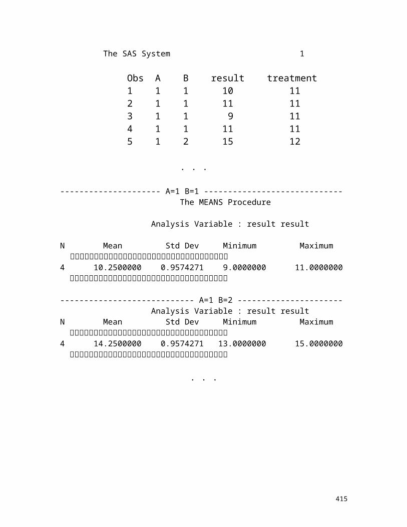
Sums of Squares
SSy: The sum of squared differences between the
observations and the grand mean (same as two-factor
crossed experiment)
1 1 1 1
2
T
K
k
J
j
n
iijk ndfyySSy
jk
SSA: Sum of squared differences between the level means
for factor A and the grand mean, weighted by the number
of experimental units for each treatment (same as for the
crossed experiment):
11 1
2
JdfyynSSAK
k
J
jjjk
SSB(A): Sum of squared differences between the level
means for Factor B with each level of Factor A, and the
mean and mean of all observations for that level of Factor
415

A, weighted by the number of experimental units for each
treatment:
)1()(2
1 1
KJdfyynASSBK
k
J
jjjkjk
SSE: Sum of squared differences between the observed
values for each experimental unit and the treatment means
(same as for crossed experiments):
K
k
J
jT
n
ijkijk JKndfyySSE
jk
1 1 1
2
416

Expected Mean Squares and F-tests for Nested Design, Both Factors Fixed: Sourc
e
SS MS EMS F
A SSA
1
JSSA
MSAA
2
* F=MSA/MSE
B (A) SSB(
A) )1()(
)(
KJASSB
AMSB)(
2
AB
**
F=MSB(A)/
MSE
Error SSE
JKnSSE
MSE
T
2
* A 2
=
112
JnK
J
jjA
when the number of observations (n)
are all equal.
417

** )(
2
AB =)1(
1 1)(
2
KJn
K
k
J
jjABk
when the number of
observations (n) are all equal.
Comparison of Factorial (Crossed) versus Nested experiments, with J=3, K=3 and njk=4 observations per treatment
Factorial Exp. Nested Exp.Source DoF Source DoFTreatment 8 Treatment 8 Factor A 2 Factor A 2 Factor B 2 Factor B(A) 6 A x B 4Error 27 Error 27Total 35 Total 35
418
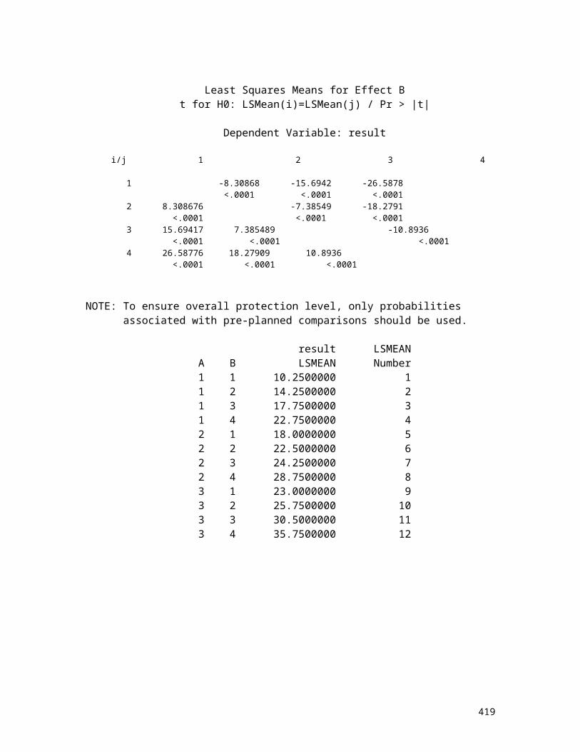
Example:
A1B1 = 10 A1B1 = 11 A1B2= 13 A2B4 = 23
A1B2 = 15 A2B3 = 18 A2B4= 25 A1B1 = 11
A2B4 = 20 A2B3 = 18 A1B1= 9 A2B3 = 18
A2B4 = 22 A1B2 = 15 A2B3 = 18 A1B2 = 14
Nested design with two factors, where the second factor is
nested in the first factor, with four replications per
treatment.
419

Data:
A B result1 1 10.001 1 11.001 1 9.001 1 11.001 2 15.001 2 15.001 2 13.001 2 14.002 3 18.002 3 19.002 3 17.002 3 18.002 4 20.002 4 22.002 4 25.002 4 23.00
420

SAS:
PROC IMPORT OUT= WORK.nested DATAFILE= “E:\frst430\lemay\examples\encyl_examples.xls" DBMS=EXCEL REPLACE; SHEET="nested$"; GETNAMES=YES; MIXED=NO; SCANTEXT=YES; USEDATE=YES; SCANTIME=YES;RUN;options ls=70 ps=50 pageno=1;
data nested2;set nested;*set up a label for each treatment, with factor a and factor b, for example, treatment of 11 is factor A of 1,and factor b of 1;treatment=(a*10)+b;lnresult=log(result);run;
proc print data=nested2;run;
proc shewhart data=nested2; boxchart result*treatment; run;
PROC GLM data=nested2;class a b;model result=a b(a);output out=glmout r=resid p=predict;lsmeans a b(a)/pdiff tdiff;run;
421

proc plot data=glmout;plot resid*predict='*';run;
PROC univariate data=glmout plot normal;Var resid;Run;PROC GLM data=nested2;class a b;model lnresult=a b(a);output out=glmout2 r=resid2 p=predict2;lsmeans a b(a)/pdiff tdiff;run;
proc plot data=glmout2;plot resid2*predict2='*';run;
PROC univariate data=glmout2 plot normal;Var resid2;Run;
422

Selected SAS Output:
The SAS System 1
Obs A B result treatment lnresult
1 1 1 10 11 2.302592 1 1 11 11 2.397903 1 1 9 11 2.197224 1 1 11 11 2.397905 1 2 15 12 2.708056 1 2 15 12 2.708057 1 2 13 12 2.564958 1 2 14 12 2.639069 2 3 18 23 2.8903710 2 3 19 23 2.9444411 2 3 17 23 2.8332112 2 3 18 23 2.8903713 2 4 20 24 2.9957314 2 4 22 24 3.0910415 2 4 25 24 3.2188816 2 4 23 24 3.13549
423

The SAS System 2
The GLM Procedure
Class Level Information
Class Levels ValuesA 2 1 2B 4 1 2 3 4
Number of Observations Read 16Number of Observations Used 16 The SAS System 3 The GLM Procedure
Dependent Variable: result result
Sum ofSource DF Squares Mean Square F ValueModel 3 328.5000000 109.5000000 64.10Error 12 20.5000000 1.7083333Corrected Total 15 349.0000000
Source Pr > F Model <.0001 Error Corrected Total
R-Square Coeff Var Root MSE result Mean0.941261 8.043275 1.307032 16.25000
424

(Type I SS not shown)
Source DF Type III SS Mean Square F ValueA 1 256.0000000 256.0000000 149.85B(A) 2 72.5000000 36.2500000 21.22
Source Pr > F A <.0001 B(A) 0.0001 The SAS System The GLM Procedure Least Squares Means
result H0:LSMean1=LSMean2A LSMEAN t Value Pr > |t|
1 12.2500000 -12.24 <.00012 20.2500000
result LSMEANB A LSMEAN Number1 1 10.2500000 12 1 14.2500000 23 2 18.0000000 34 2 22.5000000 4
425

Least Squares Means for Effect B(A)t for H0: LSMean(i)=LSMean(j) / Pr > |t|
Dependent Variable: result
i/j 1 2 3 41 -4.32801 -8.38553 -13.2545 0.0010 <.0001 <.0001
2 4.328014 -4.05751 -8.92653 0.0010 0.0016 <.0001
3 8.385528 4.057513 -4.86902 <.0001 0.0016 0.0004
4 13.25454 8.926529 4.869016 <.0001 <.0001 0.0004
NOTE: To ensure overall protection level, only probabilities associated with pre-planned comparisons should be used.
426

Plot of resid*predict. Symbol used is '*'.
resid ‚ ‚ 2.50 ˆ * 2.25 ˆ 2.00 ˆ 1.75 ˆ 1.50 ˆ 1.25 ˆ 1.00 ˆ * 0.75 ˆ * * 0.50 ˆ * 0.25 ˆ 0.00 ˆ *-0.25 ˆ * *-0.50 ˆ *-0.75 ˆ-1.00 ˆ *-1.25 ˆ * *-1.50 ˆ-1.75 ˆ-2.00 ˆ-2.25 ˆ-2.50 ˆ * ‚ Š-ˆ-----------ˆ-----------ˆ-----------ˆ-----------ˆ-----------ˆ- 10.0 12.5 15.0 17.5 20.0 22.5
predict
NOTE: 3 obs hidden.
The SAS System The UNIVARIATE Procedure Variable: resid
Some outputs removed
Tests for Normality
Test --Statistic--- --p value--Shapiro-Wilk W 0.960624 Pr<W 0.6731Kolmogorov-Smirnov D 0.135583 Pr>D >0.1500Cramer-von Mises W-Sq 0.054347 Pr>W-Sq>0.2500Anderson-Darling A-Sq 0.353872 Pr>A-Sq>0.2500
427

Stem Leaf # Boxplot 2 5 1 | 1 0 1 | 0 0058888 7 +--+--+ -0 522 3 +-----+ -1 220 3 | -2 5 1 | ----+----+----+----+
Variable: resid
Normal Probability Plot 2.5+ *+++++++ | ++++*++++ | *+**+*+++* | *+*+*+++ | ++++*++*+ -2.5++++++++* +----+----+----+----+----+----+----+----+----+----+ -2 -1 0 +1 +2
428

The SAS System 10
The GLM Procedure
Class Level Information
Class Levels Values A 2 1 2 B 4 1 2 3 4
Number of Observations Read 16Number of Observations Used 16
The SAS System The GLM Procedure
Dependent Variable: lnresult
Sum ofSource DF Squares Mean Square F Value
Model 3 1.35905142 0.45301714 73.91Error 12 0.07355155 0.00612930Corrected Total 15 1.43260297
Source Pr > F Model <.0001 Error Corrected Total
R-Square Coeff Var Root MSE lnresult Mean0.948659 2.852397 0.078290 2.744703
429

(Type I SS not shown)
Source DF Type III SS Mean Square F ValueA 1 1.04235590 1.04235590 170.06B(A) 2 0.31669552 0.15834776 25.83
Source Pr > F A <.0001 B(A) <.0001
The GLM Procedure Least Squares Means
lnresult H0:LSMean1=LSMean2A LSMEAN t Value Pr > |t|1 2.48946341 -13.04 <.00012 2.99994258
lnresult LSMEANB A LSMEAN Number
1 1 2.32390005 12 1 2.65502677 23 2 2.88959896 34 2 3.11028619 4
430

Least Squares Means for Effect B(A)t for H0: LSMean(i)=LSMean(j) / Pr > |t|
Dependent Variable: lnresult
i/j 1 2 3 4
1 -5.98141 -10.2187 -14.2051 <.0001 <.0001 <.0001
2 5.981415 -4.23727 -8.22373 <.0001 0.0012 <.0001
3 10.21869 4.237271 -3.98646 <.0001 0.0012 0.0018
4 14.20514 8.223726 3.986455 <.0001 <.0001 0.0018
NOTE: To ensure overall protection level, only probabilities associated with pre-planned comparisons should be used.
431

Plot of resid2*predict2. Symbol used is '*'.
resid2 ‚ 0.15 ˆ ‚ ‚ ‚ ‚ ‚ * 0.10 ˆ ‚ ‚ ‚ * ‚ ‚ * 0.05 ˆ * ‚ ‚ ‚ * ‚ ‚ 0.00 ˆ * ‚ ‚ * * ‚ * ‚ ‚ -0.05 ˆ ‚ * ‚ ‚ ‚ ‚ * -0.10 ˆ ‚ ‚ * ‚ * ‚ ‚ -0.15 ˆ ‚ Šˆ-----------ˆ-----------ˆ-----------ˆ-----------ˆ-----------ˆ- 2.2 2.4 2.6 2.8 3.0 3.2
predict2
NOTE: 3 obs hidden.
432

The UNIVARIATE Procedure Variable: resid2
(Some outputs deleted)
Tests for Normality
Test -Statistic--- --p Value--
Shapiro-Wilk W 0.950268 Pr<W 0.4939Kolmogorov-Smirnov D 0.150539 Pr>D >0.1500Cramer-von Mises W-Sq 0.047813 Pr>W-Sq
>0.2500Anderson-Darling A-Sq 0.321185 Pr>A-Sq
>0.2500
Stem Leaf # Boxplot 1 1 1 | 0 55577 5 +-----+ 0 003 3 *--+--* -0 222 3 +-----+ -0 96 2 | -1 31 2 | ----+----+----+----+ Multiply Stem.Leaf by 10**-1
Normal Probability Plot 0.125+ +++*+++ | * * *+*++++ | *+**+++++ | +*+*+*+ | ++++*+* -0.125+ +++*+++ * +----+----+----+----+----+----+----+----+----+----+ -2 -1 0 +1 +2
433

CRD: One Factor Experiment, Fixed Effects with
subsampling [26.7 of textbook (White)]
Example: Site Preparation
A forester would like to test whether different site preparation methods result in difference in heights. Fifteen areas each 0.02 ha in size are laid our over a fairly homogeneous area. Five site preparation treatments are randomly applied to 15 plots. One hundred trees are planted (same genetic stock and same age) in each area. At the end of 5 years, the heights of EACH seedling in each plot were measured.
We have three hierarchical levels:
Treatments Experimental units within treatments – level at which
the treatment is applied Trees within experimental units – are “nested” in
experimental units; different trees in different experimental units
We have variation: Between treatments Between experimental units within each treatment Between trees within each experimental unit in each
treatment
434

Notation
Population:
ijly = response variable measured on sample l of experimental unit i and treatment j
j=1 to J treatments
= the grand or overall mean regardless of treatmentTRj = the treatment effect
j = the mean for treatment j; grand mean plus the treatment effect
The difference between a particular measure for a sample l, an experimental unit i, and the mean for the treatment j that was applied to it is now two parts:
jijlSUijlEUij y The error for the experimental unit and the error for the sample unit in the experimental unit.
435

For the experiment:
SUijlEUijTRjijl eeyy
y = the grand or overall mean of all measures from the experiment regardless of treatment
jy = the mean of all measures for treatment j ; under error variance assumptions, will be an unbiased estimate of
TRj = the difference between the mean of experiment measures for treatment j and the overall mean of measures from all treatments
nj = the number of experimental units measured in treatment j; = n if these are all equal.
nT = the number of experimental units measured over all
treatments =
J
jjn
1; = J X n if these are all equal.
mij = the number of samples measured in experimental unit i of treatment j ; mij = m if these are all equal
mT =
J
j
n
iij
j
m1 1
the number of samples measured in
experimental unit i of treatment j ; mT = J X n X m = Jnm if these are all equal
436

Analysis Methods
Possible ways to analyze this experiment are:
1. Simplify this by calculating averages for each experimental unit and use these in the analysis of variance (would then be Completely Randomized Design: one factor, already covered)
2. Keep each sample observation, and use least squares to calculate as per CRD: one factor, but also estimate the within experimental unit variance (will cover this now)
3. Keep each sample observation, and use a mixed model and maximum likelihood, with the two “error terms” as random-effects (e.g., PROC MIXED in SAS).
Option 1 is simpler; Options 2 and 3 allow us to look at the variability within experimental unit.
Another option you will see but NOT CORRECT!! Keep each sample observation and treat this as one
experimental unit as if this was a CRD: one factor experiment.
Since the treatment was NOT applied at this level, this analysis would not be correct. Treatments are randomly assigned to the experimental unit level. The degrees of freedom and the estimated error variance used in the F-test would not be correct. In some literature, the samples are termed “pseudo-replications”.
437

We then calculate:
1) Sum of squared differences between the observed values
and the overall mean (SSy):
11
1 1
1 1 1
2
T
J
j
n
iij
J
j
n
i
m
lijl
mmdf
yySSy
j
j ij
2) Sum of squared differences between the treatment
means, and the grand mean, weighted by the number of
experimental units in each treatment (SSTR)
11
JdfyymSSJ
jj
n
iijTR
j
If the number of samples per experimental unit are all the
same (m) and the number of experimental units per
treatment are all the same (n), this becomes:
11
JdfyynmSSJ
jjTR
438

3) Sum of squared differences between the means values
for each experimental unit and the treatment means
J
jjT
J
j
n
ijijijEE
nJndf
yymSSj
1
1 1
2
)1(
If the number of samples per experimental unit are all the
same (m) and the number of experimental units per
treatment are all the same (n), this becomes:
)1(
1 1
2
nJJndf
yymSS
T
J
j
n
ijijEE
This is then experimental units nested in treatments.
439

4) Sum of squared differences between the observed values
for each experimental unit and the treatment means
)1( 1 11 1 1
2
J
j
n
iij
J
j
n
i
m
lijijlSE
jj ij
mdfyySS
If the number of samples per experimental unit are all the
same (m) and the number of experimental units per
treatment are all the same (n), this becomes:
)1( 1 1 1
2
mJndfyySSJ
j
n
i
m
lijijlSE
This is then sample units nested in experimental units and
treatments.
AND:
SEEETR SSSSSSSSy
440

Test for differences among treatment means
The main question is: Are the treatment means different? H0: 1 = 2 = … = J
H1: not all the sameOR:
What is the appropriate F-test? Need to look at the
expected mean squares.
Expected Mean Square: Treatments Fixed, and assuming the number of experimental units per treatment, and samples per experimental unit are all equal
Source df SS MS Expected Mean Squares
Treatment
J-1 SSTR MSTRAEESE m
22
Exp. Error
J(n-1) SSEE MSEE22
EESE m
SamplingError
Jn(m-1) SSSE MSSE
Total Jmn -1 SSy
441

Expected Mean Square: Treatments Random, and assuming the number of experimental units per treatment, and samples per experimental unit are all equal
Source df SS MS Expected Mean Squares
Treatment
J-1 SSTR MSTR 222
TREESE nmm
Exp. Error
J(n-1) SSEE MSEE22
EESE m
SamplingError
Jn(m-1) SSSE MSSE2
SE
Total Jmn -1 SSy
F-test is the same for Fixed-effects or Random Effects Treatments:
Source MS F p-valueTreatment
MSTR F= MSTR/MSEE
Prob F> F(J-1),( nT -J),1-
Exp.Error
MSEE
SamplingError
MSSE
Total
If )1,,1( JnJ TFF we reject H0 and conclude that there
is a difference between the treatment means.
442

Assumptions: Check residuals as other experiments. NOTE: There are also assumptions on the experimental error – could also be checked.
Tests for pairs of Means: Use experimental error as the error term rather than the default which is the sampling error.
Confidence Intervals:
jn
iij
EEdfEEj
m
MSty
1
21),(
e.g., use the mean square used for the denominator of the F-test (MSEE), and divide by the number of observations (samples) for that treatment. Degrees of freedom for the t corresponds to the df for the mean square (dfEE).
443

Example from Textbook:
Have three temperatures: low, medium, and high (J=3) For each, we have two experimental units (batches)
(n=2) Randomly assign temperatures to each batch For each batch, we have three loaves of bread (m=2) The response variable is crustiness of bread.
Data:
temp batch observation yijllow 1 1 4low 1 2 7low 1 3 5low 2 1 12low 2 2 8low 2 3 10medium 1 1 14medium 1 2 13medium 1 3 11medium 2 1 9medium 2 2 10medium 2 3 12high 1 1 14high 1 2 17high 1 3 15high 2 1 16high 2 2 19high 2 3 18
444

SAS code: Three options presented1. Using PROC GLM and the sample observations.
Model yijk= treat batch(treat);2. Using the averages for each experimental unit and
PROC GLM. Model yijk=treat;3. Using PROC MIXED, and the sample observations.
Model yijk=treat; Random batch(treat);
PROC IMPORT OUT= WORK.onesub DATAFILE= "E:\frst430\lemay\examples\ subsampling_neter_newest_p1109.xls" DBMS=EXCEL REPLACE; SHEET="data$"; GETNAMES=YES; MIXED=NO; SCANTEXT=YES; USEDATE=YES; SCANTIME=YES; RUN;
options ls=70 ps=50 pageno=1;
* Analysis 1. first, use GLM and bring in the Experimental error and the Sampling error into the design;PROC GLM data=onesub;class temp batch;model yijl=temp batch(temp);random batch(temp)/test;test h=temp e=batch(temp);lsmeans temp /e=batch(temp) pdiff tdiff;output out=glmout r=resid p=predict;run;
proc plot data=glmout;plot resid*predict='*';run;proc univariate data=glmout normal plot;var resid;run;
445

*Analysis 2. This is least squares but using the mean of all samples in each experimental unit;proc sort data=onesub;by temp batch;run;
proc means data=onesub;var yijl;by temp batch;output out=meany mean=ybars;run;
PROC GLM data=meany;class temp;model ybars=temp;lsmeans temp /pdiff tdiff;output out=glmout2 r=resid2 p=predict2;run;
proc plot data=glmout2;plot resid2*predict2='*';run;proc univariate data=glmout2 normal plot;var resid2;run;
* Analysis 3: this is using maximum likelihood for a mixed model to estimate variances and get correct F-tests;
PROC MIXED data=onesub;class temp batch;model yijl=temp;lsmeans temp/pdiff;random batch(temp);run;
446

Analysis 1: GLM using samples with experimental error given as batch(treat), and sampling error as the Error term. The SAS System 1
The GLM Procedure
Class Level Information
Class Levels Values temp 3 high low medium batch 2 1 2
Number of Observations Read 18 Number of Observations Used 18 The SAS System
The GLM Procedure
Dependent Variable: yijl yijl
Sum ofSource DF Squares Mean Square F Value
Model 5 284.4444444 56.8888889 21.79Error 12 31.3333333 2.6111111Corrected Total 17 315.7777778
Source Pr > F Model <.0001 Error Corrected Total
R-Square Coeff Var Root MSE yijl Mean
0.900774 13.59163 1.615893 11.88889
447

(NOTE: Type I SS removed)
Source DF Type III SS Mean Square F Valuetemp 2 235.4444444 117.7222222 45.09batch(temp) 3 49.0000000 16.3333333 6.26
Source Pr > F temp <.0001 batch(temp) 0.0084 NOTE: Variance components and GLM Mixed model analysis given by SAS removed – often not correct.
Least Squares MeansStandard Errors and Probabilities Calculated Using the Type III MS for batch(temp) as an Error Term
LSMEANtemp yijl LSMEAN Numberhigh 16.5000000 1low 7.6666667 2medium 11.5000000 3
Least Squares Means for Effect temp t for H0: LSMean(i)=LSMean(j) / Pr > |t|
Dependent Variable: yijl
i/j 1 2 31 3.785714 2.142857 0.0323 0.12152 -3.78571 -1.64286 0.0323 0.19903 -2.14286 1.642857 0.1215 0.1990
NOTE: To ensure overall protection level, only probabilities associated with pre-planned comparisons should be used.
448

Dependent Variable: yijl yijl
Tests of Hypotheses Using the Type III MS for batch(temp) as an Error Term
Source DF Type III SS Mean Square F Valuetemp 2 235.4444444 117.7222222 7.21
Source Pr > F temp 0.0715
Plot of resid*predict. Symbol used is '*'. resid ‚ 2.000 ˆ * ‚ ‚ 1.667 ˆ * * * ‚ ‚ 1.333 ˆ * * ‚ ‚ 1.000 ˆ ‚ ‚ 0.667 ˆ ‚ ‚ 0.333 ˆ * * ‚ ‚ 0.000 ˆ * ‚ ‚-0.333 ˆ * * * ‚ ‚-0.667 ˆ ‚ ‚-1.000 ˆ ‚ ‚-1.333 ˆ * * * ‚ ‚-1.667 ˆ * * ‚ ‚-2.000 ˆ * ‚ Šˆ---------ˆ---------ˆ---------ˆ---------ˆ---------ˆ---------ˆ- 5.0 7.5 10.0 12.5 15.0 17.5 20.0
predict
449

The UNIVARIATE Procedure Variable: residNOTE: All outputs removed except for Normality tests and box plot and normality plot
Tests for Normality
Test --Statistic--- -p Value------
Shapiro-Wilk W 0.908031 Pr<W 0.0794Kolmogorov-Smirnov D 0.17031 Pr>D >0.1500Cramer-von Mises W-Sq 0.084708 Pr>W-Sq 0.1732Anderson-Darling A-Sq 0.605378 Pr>A-Sq 0.0984
Stem Leaf # Boxplot 2 0 1 | 1 777 3 | 1 33 2 +-----+ 0 | | 0 033 3 | + | -0 333 3 *-----* -0 | | -1 333 3 +-----+ -1 77 2 | -2 0 1 | ----+----+----+----+
The UNIVARIATE Procedure Variable: resid
Normal Probability Plot 2.25+ +++* | * *+*+ | * *++++ 0.75+ ++++ | +**+* | *+** -0.75+ ++++ | +++** * | * +*+* -2.25+ ++++ +----+----+----+----+----+----+----+----+----+----+ -2 -1 0 +1 +2
450

Analysis 2: GLM using averages for each sample unit experimental error is now the Error term. The SAS System The MEANS Procedure
-------------- temp=high batch=1 ------------------
Analysis Variable : yijl yijl
N Mean Std Dev Minimum Maximum-------------------------------------------------3 15.3333333 1.5275252 14.0000000 17.0000000-------------------------------------------------
--------------- temp=high batch=2 -------
Analysis Variable : yijl yijl
N Mean Std Dev Minimum Maximum-------------------------------------------------3 17.6666667 1.5275252 16.0000000 9.0000000-------------------------------------------------
--------------------- temp=low batch=1 -------
Analysis Variable : yijl yijl
N Mean Std Dev Minimum Maximum------------------------------------------------- 3 5.3333333 1.5275252 4.0000000 7.0000000---------------------------------------------------
451

----------------- temp=low batch=2 ------- Analysis Variable : yijl yijl
N Mean Std Dev Minimum Maximum-------------------------------------------------3 10.0000000 2.0000000 8.0000000 12.0000000---------------------------------------------------
--------------------- temp=medium batch=1 ---------
Analysis Variable : yijl yijl N Mean Std Dev Minimum Maximum------------------------------------------------- 3 12.6666667 1.5275252 11.0000000 14.0000000-------------------------------------------------
----------------- temp=medium batch=2 -------------
Analysis Variable : yijl yijl
N Mean Std Dev Minimum Maximum------------------------------------------------- 3 10.3333333 1.5275252 9.0000000 12.0000000---------------------------------------------------
452

The SAS System
The GLM Procedure
Class Level Information
Class Levels Values temp 3 high low medium batch 2 1 2
Number of Observations Read 6 Number of Observations Used 6 The GLM Procedure
Dependent Variable: ybars yijl
Sum ofSource DF Squares Mean Square F ValueModel 2 78.48148148 39.24074074 7.21Error 3 16.33333333 5.44444444Corrected Total 5 94.81481481
Source Pr > F Model 0.0715 Error Corrected Total
R-Square Coeff Var Root MSE ybars Mean
0.827734 19.62617 2.333333 11.88889
453

NOTE: Type I SS removed from the SAS outputs.
Source DF Type III SS Mean Square F Valuetemp 2 78.48148148 39.24074074 7.21
Source Pr > F temp 0.0715 The SAS System
LSMEANtemp ybars LSMEAN Number
high 16.5000000 1low 7.6666667 2medium 11.5000000 3
Least Squares Means for Effect temp t for H0: LSMean(i)=LSMean(j) / Pr > |t|
Dependent Variable: ybars
i/j 1 2 3
1 3.785714 2.142857 0.0323 0.12152 -3.78571 -1.64286 0.0323 0.19903 -2.14286 1.642857 0.1215 0.1990
NOTE: To ensure overall protection level, only probabilities associated with pre-planned comparisons should be used.
454

The SAS System
Plot of resid2*predict2. Symbol used is '*'.
resid2 ‚ ‚ 2.333 ˆ * ‚ ‚ ‚ ‚ ‚ ‚ 1.167 ˆ * * ‚ ‚ ‚ ‚ ‚ ‚ 0.000 ˆ ‚ ‚ ‚ ‚ ‚ ‚-1.167 ˆ * * ‚ ‚ ‚ ‚ ‚ ‚-2.333 ˆ * ‚ Šˆ---------ˆ---------ˆ---------ˆ---------ˆ---------ˆ---------ˆ- 6 8 10 12 14 16 18
predict2
455
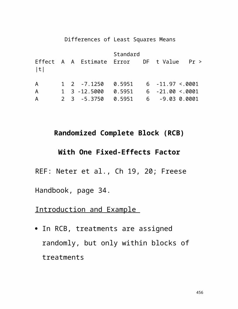
The UNIVARIATE Procedure Variable: resid2
NOTE: removed all but the normality tests and normality plots. Tests for Normality
Test --Statistic--- --p Value------Shapiro-Wilk W 0.912907 Pr<W 0.4558Kolmogorov-Smirnov D 0.240697 Pr>D >0.1500Cramer-von Mises W-Sq 0.06404 Pr>W-Sq >0.2500Anderson-Darling A-Sq 0.352911 Pr>A-Sq >0.2500
The UNIVARIATE Procedure Variable: resid2
Normal Probability Plot 2.5+ +*+++ | * *+++++ | ++++++ | +++++ | +++++* * -2.5+ +++*+ +----+----+----+----+----+----+----+----+----+----+ -2 -1 0 +1 +2
456

Analysis 3: MIXED using each sample unit value.
The SAS System The Mixed Procedure
Model InformationData Set WORK.ONESUBDependent Variable yijlCovariance Structure Variance ComponentsEstimation Method REMLResidual Variance Method ProfileFixed Effects SE Method Model-BasedDegrees of Freedom Method Containment Class Level Information
Class Levels Values temp 3 high low medium batch 2 1 2
Dimensions Covariance Parameters 2 Columns in X 4 Columns in Z 6 Subjects 1 Max Obs Per Subject 18
Number of Observations Number of Observations Read 18 Number of Observations Used 18 Number of Observations Not Used 0
457

Iteration History
Iteration Evaluations -2 Res Log Like Criterion0 1 73.11545106 1 1 67.84036856 0.00000000
Convergence criteria met.
Covariance Parameter Estimates Cov Parm Estimate batch(temp) 4.5741 Residual 2.6111
Fit Statistics -2 Res Log Likelihood 67.8 AIC (smaller is better) 71.8 AICC (smaller is better) 72.8 BIC (smaller is better) 71.4
Type 3 Tests of Fixed Effects Num DenEffect DF DF F Value Pr > Ftemp 2 3 7.21 0.0715 Least Squares Means
StandardEffect temp Estimate Error DF t Value Pr>|t|temp high 16.5000 1.6499 3 10.00 0.0021temp low 7.6667 1.6499 3 4.65 0.0188temp medium 11.5000 1.6499 3 6.97 0.0061
458

Differences of Least Squares Means
StandardEffect temp temp Estimate Error DF t Value Pr>|t|temp high low 8.8333 2.3333 3 3.79 0.0323temp high medium 5.0000 2.3333 3 2.14 0.1215temp low medium -3.8333 2.3333 3 -1.64 0.1990
459

RCB: One Factor Experiment, Fixed Effects with
subsampling
Blocked (random or fixed-effect, usually random) Fixed-effect factor A (we will label this as TR for
treatment) Experimental units – level at which the block
with factor A combinations are applied; may be one experimental unit or more than one (generalized RCB or RCB with replicates)
Sampling units – number of items measured within each experimental unit.
Notation for a Generalized RCB with subsampling:
Population: = response variable measured on sample l of
experimental unit i, block j, and treatment k
The difference between a particular measure for a sample l, an experimental unit i, and the mean for the block j and treatment k combination that was applied to it is now two parts:
The error for the experimental unit and the error for the sample unit in the experimental unit.
460

For the experiment:
= the grand or overall mean of all measures from the experiment regardless of treatment
= the mean of all measures for block j and treatment k ; under error variance assumptions, will be an unbiased estimate of
= the mean of all measures for block j will be an unbiased estimate of
= the mean of all measures for treatment k will be an unbiased estimate of
njk = the number of experimental units measured in each combination of block by treatment; = n if these are all equal.
nT = the number of experimental units measured over all treatments = ; = J X K X n if these are all equal.
mijk = the number of samples measured in experimental unit i of treatment and block jk ; mijk = m if these are all equalmT = the number of samples measured in experimental unit i of treatment j ; mT = J X K X n X m = JKnm if these are all equal
461

Analysis Methods
Possible ways to analyze this experiment are:
4. Simplify this by calculating averages for each experimental unit and use these in the analysis of variance (would then be Generalized Randomized Complete Block Design: one factor, already covered)
5. Keep each sample observation, and use least squares or to calculate as per Generalized Random Complete Block: one factor, but also estimate the within experimental unit variance (will cover this now)
6. Keep each sample observation, and use a mixed model and maximum likelihood, with the two “error terms” as random-effects (e.g., PROC MIXED in SAS).
Option 1 is simpler; Options 2 and 3 allow us to look at the variability within experimental unit.
Another option you will see but NOT CORRECT!! Keep each sample observation and treat this as one
experimental unit Since the treatment was NOT applied at this level, this
analysis would not be correct. Treatments are randomly assigned to the experimental unit level. The degrees of freedom and the estimated error variance used in the F-test would not be correct. In some literature, the samples are termed “pseudo-replications”.
462

We then calculate:
For a Generalized Randomized Complete Block design with one-
factor, and subsampling of the experimental units.
Main Questions:
1. For the generalized RCB, we can look at interactions between blocks and the treatment (cannot, if there is only one experimental unit per treatment and block combination with the more simpler RCB, since the interaction is the exp. unit error.). Test this first.
2. Then, if no interaction, test if there is a difference among the Factor A levels (the treatment).
3. Not really interested in the blocks.
What is the appropriate F-test? Need to look at the
expected mean squares.
463
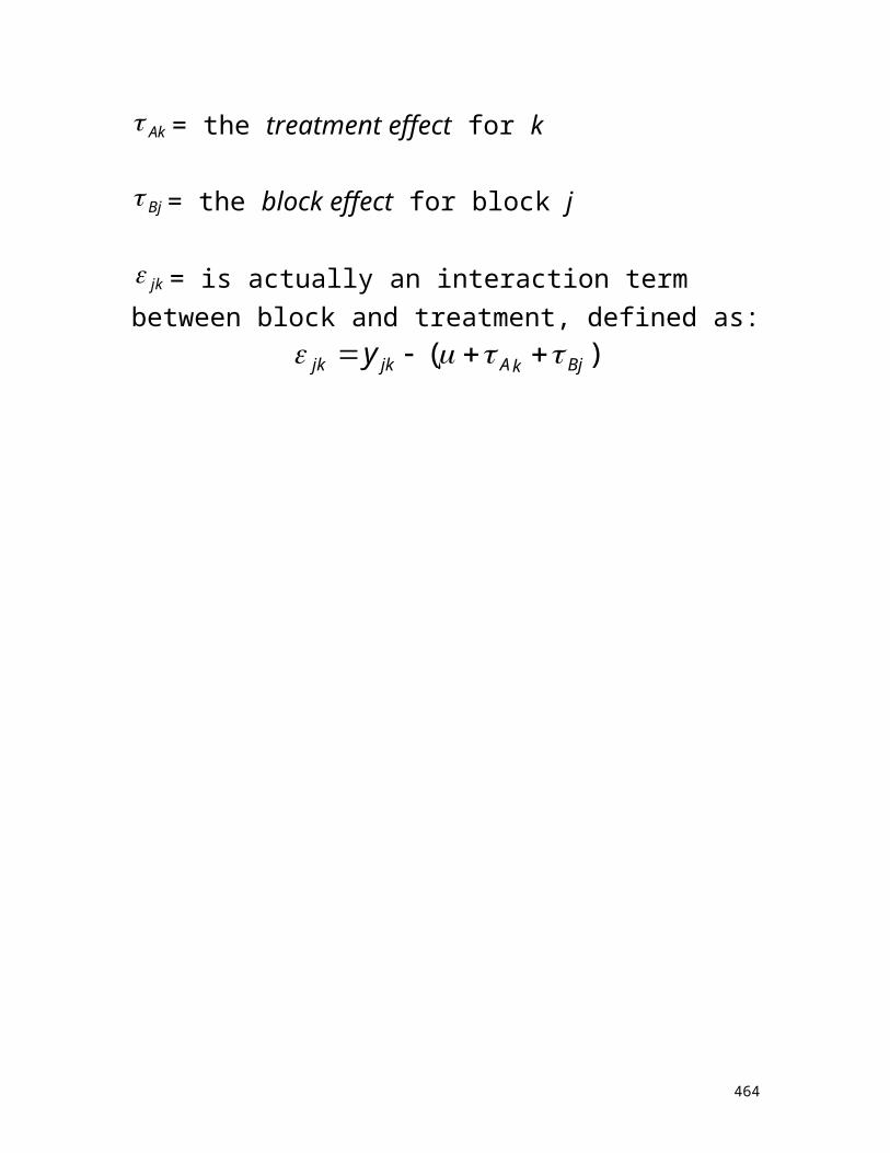
Expected Mean Square: Treatments and Blocks BOTH Fixed, and assuming the number of experimental units per treatment, and samples per experimental unit are all equal
Source df SS MS Expected Mean Squares
Block J-1 SSBLK MSBLK
Treatment
K-1 SSTR MSTR
Block X Treatment
(J-1)(K-1) SSBLK
X TR
MSBLK
X TR
Exp. Error
JK(n-1) SSEE MSEE
SamplingError
JKn(m-1) SSSE MSSE
Total JKnm -1 SSy
464

Expected Mean Square: Treatments Fixed, but Blocks are Random, and assuming the number of experimental units per treatment, and samples per experimental unit are all equal
Source df SS MS Expected Mean Squares Block J-1 SSBLK MS
BLK
Treatment K-1 SSTR MSTR
Block X Treatment
(J-1)(K-1) SSBLK X
TR
MSBLK
X TR
Exp. Error
JK(n-1) SSEE MSEE
SamplingError
JKn(m-1) SSSE MSSE
Total JKnm -1 SSy
465

Assumptions: Check residuals as other experiments. NOTE: There are also assumptions on the experimental error – could also be checked.
Tests for pairs of Means: Use experimental error as the error term rather than the default which is the sampling error.
Confidence Intervals: both Blocks and Treatments are fixed:
e.g., use the mean square used for the denominator of the F-test (MSEE), and divide by the number of observations (samples) for that Factor level k. Degrees of freedom for the t corresponds to the df for the mean square (dfEE).
Confidence Intervals: Blocks Random and Treatments are fixed:
466
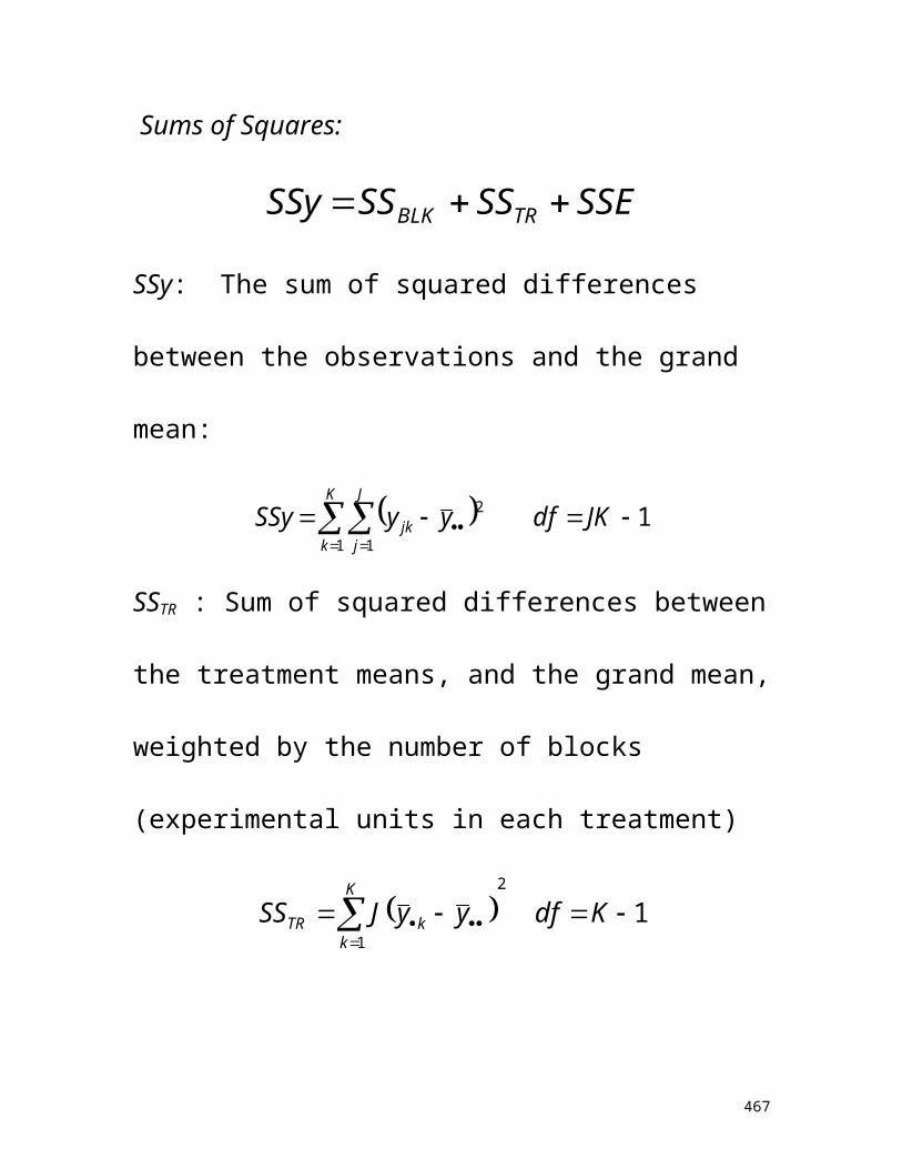
Analysis of Covariance (ANCOVA)
For experimental designs covered so far:
The response variable (y) is a continuous variable
A number of class variables (x’s) are used (effects) to
explain the variation in the response variable, via a linear
model
We are interested in differences in means for each class
variable (fixed-effects) or in the variance in the response
variable that is due to the class variable (random-effects).
For example, for CRD: two factors, mixed, we were
interested in:
Whether there is an interaction between Factor A and
Factor B.
If there is no interaction
o whether the means for levels of Factor A differ,
and if so, which ones differ?
o and whether Factor B accounts for some of the
variability in the response variable, and if so, how
much?
467

For linear regression analysis, covered in the beginning of
the course:
The dependent variable (y) is a continuous variable
A number of continuous predictor variables (x’s) are
used to explain the variation in the dependent variable in
a linear equation.
We also introduced class variables (x’s also) to help
explain the variation in the dependent variable,
represented by:
o Dummy variables to alter the intercept
o Interactions between dummy variables and
continuous predictor variable to alter the slope.
468

Analysis of covariance is an experimental design, where we
add continuous explanatory variables (called covariates) to
help explain the variability in the response variable, for
example:
Record the initial weight of all fish prior to adding
different foods. Use this initial weight as a covariate
Record soil moisture of all plots in a field prior to
applying different treatments. Use this soil moisture
as a covariate.
The covariates help “even-out” conditions that we were not
able to control in trying to obtain homogeneous treatment
units, and explain some of the variation in the response
variable.
Blocking does this in a similar fashion, but:
Blocking restricts the randomization of treatments to
experimental units (treatments assigned randomly within
blocks)
Blocks are class variables.
469

This is very similar to using continuous and class variables
in regression analysis to explain the variation in the
dependent variable, except:
We have an experiment, and we are trying to assign
cause and effect
For analysis of covariance:
o the slopes are considered the same over all
treatments (common slope), in order to assess the
impacts of different factors (called homogeneity
of slopes)
o This means that the treatment does not affect the
relationship (linear trend) between y and x
o This must be tested, as the slope of y versus x
may vary by treatment
We use these covariates to “adjust” the factor level
means to a common value (usually the mean) of the
covariate.
470

Example:
UBC would like to evaluate three ways of teaching basic statistics: (A) stats dept. method (3 lectures), (B) computer method (3 lectures plus lab using statistical software with no lab write-up), (C) applied science method (3 lectures plus written lab). “Success” is measured as a grade in a common examination for all students.
The response (exam grade) might be related to abilities before taking the course: Grade in Math 12 is used as a covariate (x variable)
and obtained for each student. Then students are randomly assigned to one of the
three class types.
The Math 12 grade is then used to “adjust” the grade in the
common exam.
471

Looking at the trends, between Mark in Stats (y) versus Mark in Grade 12 math(x), the slopes appear to be similar.
60
65
70
75
80
85
90
95
60 70 80 90 100
Mark in Grade 12 Math
Mar
k in
Sta
tistic
s
ABCC
A
C
B
Ignoring the Grade 12 March, the mark in Statistics is higher for A, and B and C are similar.
60
65
70
75
80
85
90
95
60 70 80 90 100
Mark in Grade 12 Math
Mar
k in
Sta
tistic
s
A B C
472
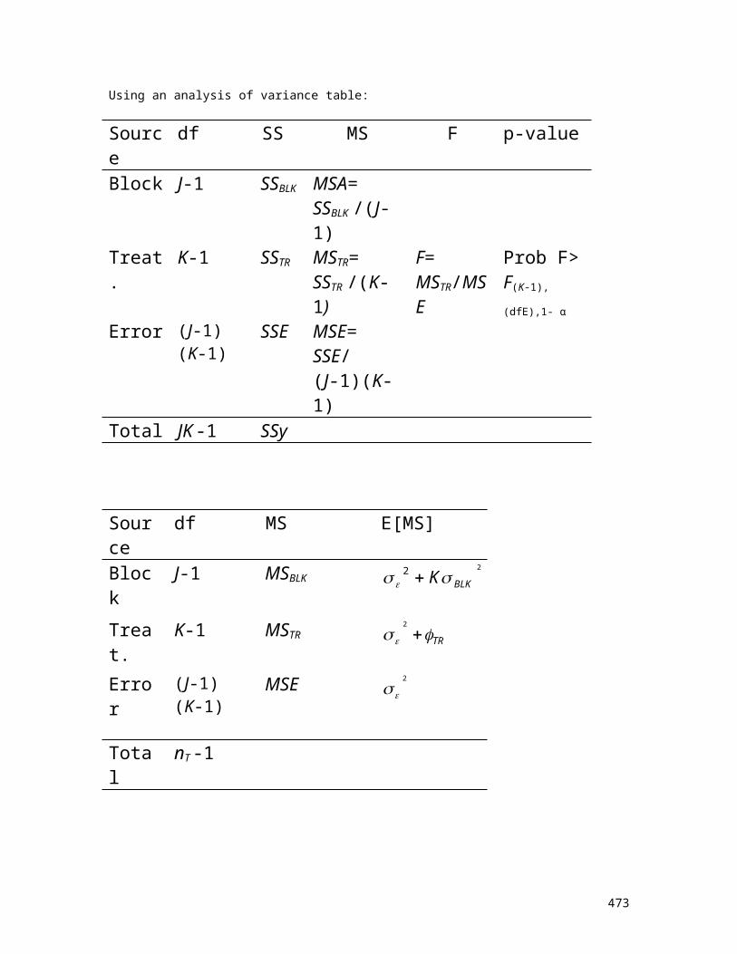
Using the
covariate, and
adjusting the
means along the y
vs x trend line to
the average Mark
in Grade 12 Math,
C and A are
similar, and B is
different60
65
70
75
80
85
90
95
60 70 80 90 100Mark in Grade 12 Math
Mar
k in
Sta
tistic
sC AB
If the Math grade was not used as a covariate, the conclusion
would be much different.
473

Model:
We add a covariate to whichever experimental design we wish to use.
For example, using an RCB with two fixed-effect factors, we add in the covariate.
Population:
jkly = response variable measured on block j and treatment kl
j=1 to J blocks; k=1 to K levels for Factor A; l=1 to L levels for Factor B; and definition of terms follows other designs.
xjkl is a measurement of the covariate for a particular experimental unit, standardized around the mean of x over all observations, as this can be easier to interpret; β is the slope of the line between y and x.
The expected mean squares are the same as the design without the covariate.
The covariate will take up one degree of freedom from the error term.
Variations in ANCOVA:
474
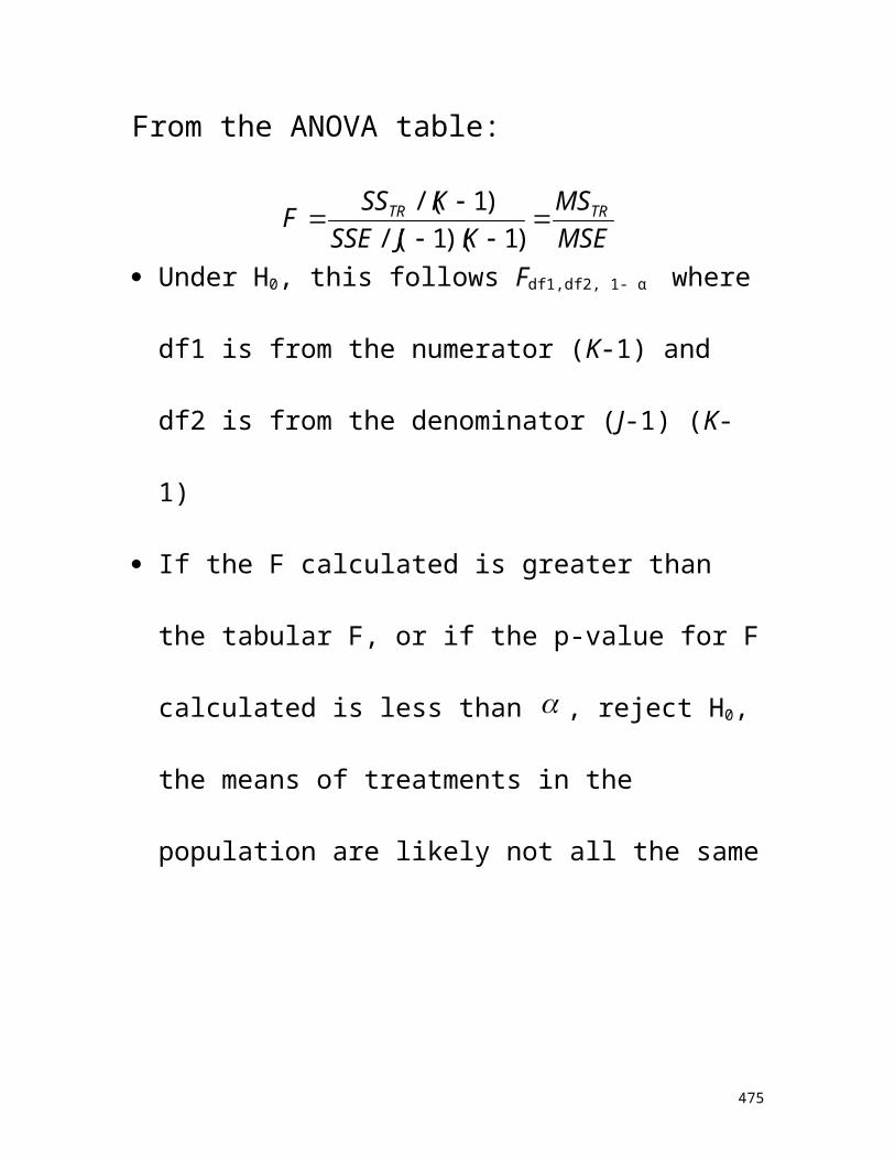
1. More than one covariate. Can add in more than one
continuous variable.
Must check for ANY interactions between continuous
variables and each of the class variables (effects) in the
experiment.
Each covariate will have a df of 1 (like a continuous
variable in regression), and this will be taken away from
the error term df.2. Slopes are not equal
y
60
65
70
75
80
85
90
95
60 70 80 90 100
x
475

Interactions between class variables and continuous variables
are significant. Can test these using partial F-tests as we did
for regression using dummy variables to represent classes.
Get generalized linear models (GLM) results for all class
variables (blocks, factors, interactions, etc.), all continuous x-
variables (covariates) , and interactions between covariates
and all class variables [full model]
o Record the df(model) and df(error) [full]
o Record the SSmodel (includes all class and continuous
variables and interactions) and SSerror [full]
Get generalized linear models results for all class variables
(blocks, factors, interactions, etc.), all continuous x-variables
(covariates) [reduced model]
o Record the df(model) and df(error) [reduced]
o Record the SSmodel and SSerror [reduced]
476

)((s))n variableinteractiodroppedtodue(
))(()()(
OR))((
)()(
fullMSE/rSS
fulldferrorSSErfullSSEreducedSSEFpartial
fulldferrorSSErreducedSSregfullSSregFpartial
Where r is the number of x-variables that were dropped. Equals:
(1)the model degrees of freedom for the full model minus the
model degrees of freedom for the reduced model, OR (2) the
error degrees of freedom for the reduced model, minus the error
degrees of freedom for the full model)
Under H0, this follows an F distribution for a 1- α/2 percentile
with r and n-m-1 (full model) degrees of freedom.
If the F for the fitted equation is larger than the F from the
table, we reject H0 (not likely true). There are different
slopes (relationship between y and x) for different treatments
(combinations of the class variable levels)
477

Harder to interpret, as with any interaction
o Use graphs to show relationships
o Switch to a regression approach to finding equations
using the continuous and class variables (represented
as dummies) and interpret these results.
(Assignment 8 as the example during class)
478

Expected Mean Squares to get called components of variance
1. Get these from a book where they are already determined for
your type of design. Must know which of your factors are
fixed and which are random.
2. Use the EMS rules to determine these. Expected Means
Squares “rules”: Appendix D of text (white or blue editions)
479

Calculation of Expected Mean Squares Using an Example
Steps to Derive Expected Mean Squares.1. Write up linear model. For example, RCB with more
than one experiment unit for each treatment within a block (generalized RCB):
)( jkijkTRBLKkTRjBLKijky
for j=1 to J, k=1 to K, i=1 to n(blocks) (treatments) (replications)
NOTE: will use instead:for j=1 to b, k=1 to t, i=1 to n(blocks) (treatments) (replications)
Then b is taken from B possible blocks;t is taken from T possible treatments;n is taken from N possible replicates within each jk. Since the replicates are nested within each Treament /Block combination, we have added brackets to indicate this.
480
Note brackets added around jk
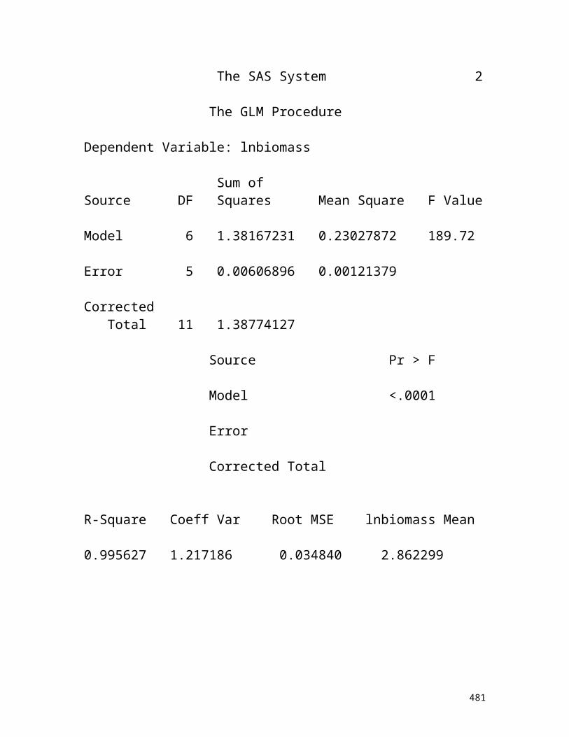
2. Generate table of indices and number of factor levels etc.
n b tEffect i j k
BLKj
TRk
BLK X TRjki(jk)
3. Indicate which effects are fixed versus random and add a symbol for each component. Note that we will use the symbol for variance (random-effects) for all components, and change this to TR for the fixed-effects treatment at the end.
Type: R R Fn b t
Effect i j k SymbolBLKj
2
BLKTRk
2
TRBLK X TRjk 2
TRBLKi(jk)
2
481

4. Fill in the table by:a. Put down a “1”, where subscript is bracketed
(nested)Type: R R F
n b tEffect i j k Symbol
BLKj2
BLKTRk
2
TRBLK X TRjk 2
TRBLKi(jk) 1 1 2
b. For each effect, put down the end value (e.g., t for number of treatments in the experiment) for each subscript that does not appear for the effect
Type: R R Fn b t
Effect i j k SymbolBLKj n t 2
BLKTRk n b 2
TRBLK X TRjk n 2
TRBLKi(jk) 1 1 2
482

c. Add the “finite population correction factor” for each of the other factors: e.g., for Blocks, this is
Bb
BbB 1
Type: R R Fn b t
Effect i j k SymbolBLKj n
Bb1 t 2
BLK
TRk n b
Tt1
2
TR
BLK X TRjk n
Bb1
Tt1
2
TRBLK
i(jk)
Nn1 1 1 2
483

5. Change FPC values to either 1 or zero.a. If factors are random and there is a very large
number of available levels, e.g., N≈∞, and B≈∞. Thus FPC→1
b. If factors are fixed, then the number of available factors is the number of factors sampled, e.g., T=t. Thus, FPC→0
c. If factors are random and there is a finite number of available factors, then no change is made (we will assume we have none of these).
Type: R R Fn b t
Effect i j k SymbolBLKj n 1 t 2
BLKTRk n b 0 2
TRBLK X TRjk n 1 0 2
TRBLKi(jk) 1 1 1 2
484

6. Write up componentsa. For each effect, select all the row(s) with effects
that contain the same subscript(s) b. Ignore any columns with the heading for that
(those) subscript(s). (i.e., select all columns that do not have the subscript.
c. Add up the product of the remaining columns for the selected row(s)
For Blocks, the subscript is j:
Type: R R Fn b t
Effect i j k SymbolBLKj n 1 t 2
BLKTRk n b 0 2
TRBLK X TRjk n 1 0 2
TRBLKi(jk) 1 1 1 2
For Block, the E[MSBLK] is: 22
BLKnt
485

For Treatment, the subscript is k:
Type: R R Fn b t
Effect i j k SymbolBLKj n 1 t 2
BLKTRk n b 0 2
TRBLK X TRjk n 1 0 2
TRBLKi(jk) 1 1 1 2
For Treatment, the E[MSTR] is: 222
TRBLKTR nnb
BUT Treatment is a fixed-effect (want to estimate the effects due to treatment, rather than the variance due to
treatment). Using the TR instead, the E[MSTR] is, therefore:
22 TRBLKTR n
Note:The interaction remains Random with a variance symbol, as this is the interaction between blocks and treatments. Since one of these is a random-effect, this is random.
486

For Block X Treatment, the subscript is jk:
Type: R R Fn b t
Effect i j k SymbolBLKj n 1 t 2
BLKTRk n b 0 2
TRBLK X TRjk n 1 0 2
TRBLKi(jk) 1 1 1 2
For Block Treatment, the E[MSBLK X TR] is: 22
TRBLKn
487

For the error term, the subscript is ijk:Type: R R F
n b tEffect i j k Symbol
BLKj n 1 t 2
BLKTRk n b 0 2
TRBLK X TRjk n 1 0 2
TRBLKi(jk) 1 1 1 2
The E[MSE] is simply: 2
For the ANOVA table then: Using j=1 to J blocks; k=1 to K treatments; and assuming all nij are equal to n (as per the notes on Generalized RCB):
Source df MS p-value E[MS] BLK J-1 MSBLK Prob F>
F(J-1),(dfE), 1- α
22BLKKn
TR K-1 MSTR Prob F> F(K-1),(dfBXT),1- α
TRTBn 22
BLKX TR
(J-1)(K-1)
MSBXT Prob F> F dfBXT,dfE,,1- α
TBn 22
Error nT -JK MSE 2
Total nT -1
488

More complex example: RCB, two-factors, split-plot. Factor B is in split-plots (subdivided experimental units):
1. Write up linear model.
)( jlkBklABljkABLKkAjBLKjkly
for j=1 to J, k=1 to K, l=1 to L (blocks) (Factor A) (Factor B)
NOTE: will use instead:for j=1 to b, k=1 to fA , l=1 to fB (blocks) (Factor A) (Factor B)
Then b is taken from B possible blocks;fA is taken from FA possible levels of Factor A;fB is taken from FB possible levels of Factor B.
The other interactions BLK X B
BLK X A X Bare combined in the error term in this model. We will separate these out to calculate the EMS:
ABjklBLKBjlBLKjkl
489

Steps 2 and 3: Generate table of indices and number of factor levels etc. Indicate which factors are fixed versus random and add a symbol for each component. Note that we will use the symbol for variance (random-effects) for all components, and change this to BA , for the fixed-effects treatment at the end.
Type: R F Fb fA fB
Effect j k l SymbolBLKj
2
BLKAk
2
ABLK X Ajk 2
ABLKBk
2
BABkl 2
ABBLK X Bjk 2
BBLKBLK X ABjkl 2
ABBLK
490

4. Fill in the table by:a. Put down a “1”, where subscript is bracketed
(nested)b. For each effect, put down the end value (e.g., fA for
number of levels of Factor A) for each subscript that does not appear for the effect
Type: R F Fb fA fB
Effect j k l SymbolBLKj fA fB 2
BLKAk b fB
2
ABLK X Ajk fB
2
ABLKBk b fA 2
BABkl b 2
ABBLK X Bjl fA
2
BBLKBLK X ABjkl 2
ABBLK
491

c. Add the “finite population correction factor” for each of the other factors: e.g., for Blocks, this is
Bb
BbB 1
Type: R F Fb fA fB
Effect j k l SymbolBLKj
Bb1 fA fB 2
BLK
Ak b
A
A
Ff
1 fB2
A
BLK X Ajk
Bb1
A
A
Ff
1 fB2
ABLK
Bk b fA
B
B
Ff
12
B
ABkl b
A
A
Ff
1
B
B
Ff
12
AB
BLK X Bjk
Bb1 fA
B
B
Ff
12
BBLK
BLK X ABjkl
Bb1
A
A
Ff
1
B
B
Ff
12
ABBLK
492

5. Change FPC values to either 1 or zero.a. If factors are random and there is a very large
number of available levels, e.g., B≈∞. Thus FPC→1
b. If factors are fixed, then the number of available factors is the number of factors sampled, e.g., fA = FA. Thus, FPC→0
c. If factors are random and there is a finite number of available factors, then no change is made (we will assume we have none of these).
Type: R F Fb fA fB
Effect j k l SymbolBLKj 1 fA fB 2
BLKAk b 0 fB
2
ABLK X Ajk 1 0 fB
2
ABLKBk b fA 0 2
BABkl b 0 0 2
ABBLK X Bjk 1 fA 0 2
BBLKBLK X ABjkl 1 0 0 2
ABBLK
493

6. Write up componentsa. For each effect, select all the row(s) with effects
that contain the same subscript(s) b. Ignore any columns with the heading for that
(those) subscript(s). (i.e., select all columns that do not have the subscript.
c. Add up the product of the remaining columns for the selected row(s)
For Blocks, the subscript is j.Type: R F F
b fA fB Effect j k l Symbol
BLKj 1 fA fB 2
BLKAk b 0 fB
2
ABLK X Ajk 1 0 fB
2
ABLKBk b fA 0 2
BABkl b 0 0 2
ABBLK X Bjk 1 fA 0 2
BBLKBLK X ABjkl 1 0 0 2
ABBLK
For Block, the E[MSBLK] is: 2
BLKBA ff
494

For Factor A, the subscript is k:
Type: R F Fb fA fB
Effect j k l SymbolBLKj 1 fA fB 2
BLKAk b 0 fB
2
ABLK X Ajk 1 0 fB
2
ABLKBk b fA 0 2
BABkl b 0 0 2
ABBLK X Bjk 1 fA 0 2
BBLKBLK X ABjkl 1 0 0 2
ABBLK
For Factor A, the E[MSA] is: 22
ABLKBAB fbf Since Factor A is a fixed-effect, using the A instead, the E[MSA] is, therefore:
2TRBLKBA f
Note:The interaction remains Random with a variance symbol, as this is the interaction between blocks and treatments. Since one of these is a random-effect, this is also a random-effect.
495

For Block X Factor A, the subscript is jk:Type: R F F
b fA fB Effect j k l Symbol
BLKj 1 fA fB 2
BLKAk b 0 fB
2
ABLK X Ajk 1 0 fB
2
ABLKBk b fA 0 2
BABkl b 0 0 2
ABBLK X Bjk 1 fA 0 2
BBLKBLK X ABjkl 1 0 0 2
ABBLK
For Block by Factor A, the E[MSBLK X A] is: 2
TRBLKBf
This was simply called “Error 1” ( 21 ) on the notes for
split plot.
496

For Factor B, the subscript is l:Type: R F F
b fA fB Effect j k l Symbol
BLKj 1 fA fB 2
BLKAk b 0 fB
2
ABLK X Ajk 1 0 fB
2
ABLKBk b fA 0 2
BABkl b 0 0 2
ABBLK X Bjl 1 fA 0 2
BBLKBLK X ABjkl 1 0 0 2
ABBLK
For Factor B, the E[MSB] is: 22
BBLKABA fbf Since Factor B is a fixed-effect, using the B instead, the E[MSB] is, therefore:
2BBLKAB f
497
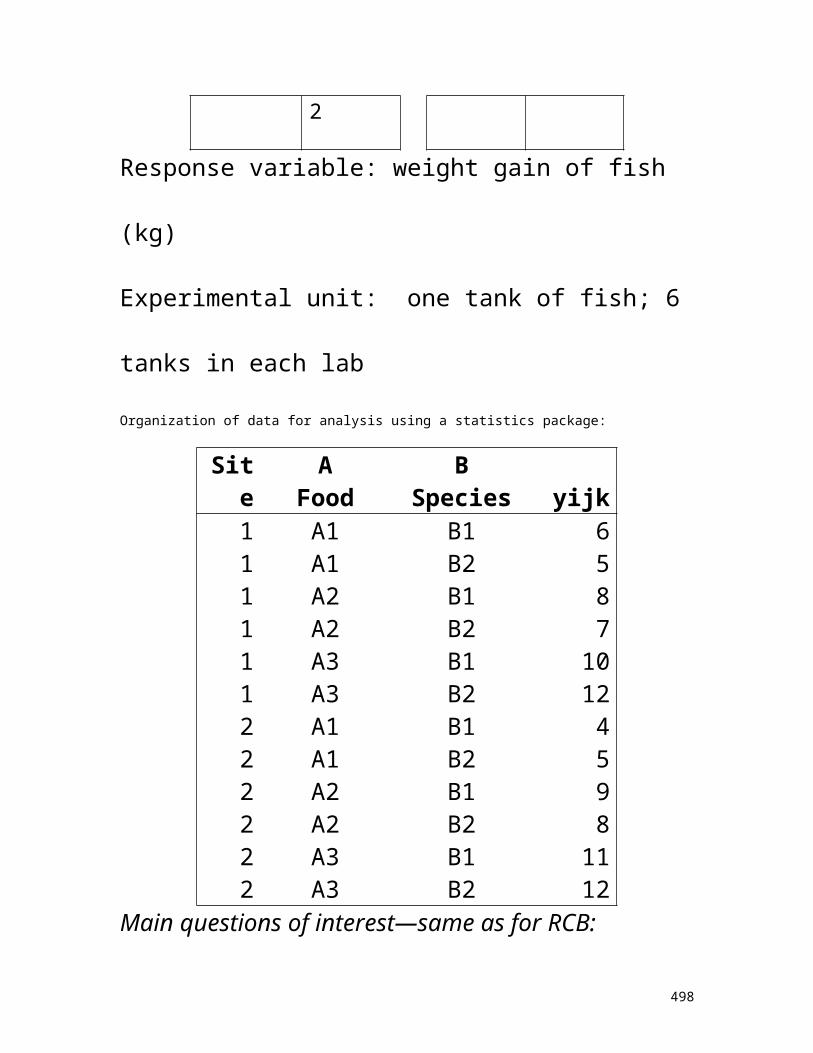
For Factor A X Factor B, the subscript is kl:
Type: R F Fb fA fB
Effect j k l SymbolBLKj 1 fA fB 2
BLKAk b 0 fB
2
ABLK X Ajk 1 0 fB
2
ABLKBk b fA 0 2
BABkl b 0 0 2
ABBLK X Bjl 1 fA 0 2
BBLKBLK X ABjkl 1 0 0 2
ABBLK
For Factor A by Factor B, the E[MSAB] is: 22
ABBLKABb Since Factor A and Factor B are both fixed-effects, using the BA instead, the E[MSAB] is, therefore:
2ABBLKBA
498

For Block X Factor B, the subscript is jl:
Type: R F Fb fA fB
Effect j k l SymbolBLKj 1 fA fB 2
BLKAk b 0 fB
2
ABLK X Ajk 1 0 fB
2
ABLKBk b fA 0 2
BABkl b 0 0 2
ABBLK X Bjl 1 fA 0 2
BBLKBLK X ABjkl 1 0 0 2
ABBLK
For Block by Factor B, the E[MSBLK X B] is: 2
BBLKAf
499

For the error term, the subscript is jkl:
Type: R F Fb fA fB
Effect j k l SymbolBLKj 1 fA fB 2
BLKAk b 0 fB
2
ABLK X Ajk 1 0 fB
2
ABLKBk b fA 0 2
BABkl b 0 0 2
ABBLK X Bjl 1 fA 0 2
BBLKBLK X ABjkl 1 0 0 2
ABBLK
The E[MSBLK X AB] is simply: 2ABBLK .
“Error 2” is a combination of BLK X B with BLK X AB, which is:
2222 ABBLKBBLKAf
Assuming no interaction between Blocks and Factor B, this 22
2 ABBLK
500

For the ANOVA table then: Using j=1 to J blocks; k=1 to K Factor A levels; l=1 to L Factor B levels; and using error 1 and error 2 (as per the notes RCB Split-Plot):
Source df MS Both A and B are Fixed; Blocks are Random
Block J-1 MSBLK2
BLKKL
Factor A K-1 MSAAL
2
1
Exp. Err. #1 (J-1)(K-1) MSE12
1L
Factor B L-1 MSBB
2
2
A x B (K-1)(L-1)
MSAXBBA
2
2
Exp. Err. #2 K(J-1)(L-1)
MSE22
2
Total JKL-1
501

Generalized RCB, one-fixed factor with subsampling. Blocks assumed fixed.
1. Write up linear model.
)()( ijkljkijkTRBLKkTRjBLKijkly
for j=1 to J, k=1 to K, (blocks) (Treatment=Factor A) i=1 to n, (Exp. units in jk)and l=1 to m (sampling in each exp. unit)
NOTE: will use instead:for j=1 to b, k=1 to fA (blocks) (Factor A) Then b is taken from B possible blocks;fA is taken from FA possible levels of Factor A;n is taken from N possible experimental units;m is taken from M possible samples in each experimental unit.
The first error term, is the EU error; the second error term is the SU error.
502

Steps 2 and 3: Generate table of indices and number of factor levels etc. Indicate which factors are fixed versus random and add a symbol for each component. Note that we will use the symbol for variance (random-effects) for all components, and change this to for the fixed-effects treatment at the end.
Type: F F R Rb fA n m
Effect j k i l SymbolBLKj
2
BLKTRk
2
TRBLK X TRjk 2
TRBLKi(jk)
2
EEl(ijk)
503

4. Fill in the table by:a. Put down a “1”, where subscript is bracketed
(nested)b. For each effect, put down the end value (e.g., fA
for number of levels of Factor A) for each subscript that does not appear for the effect
Type: F F R Rb fA n m
Effect j k i l SymbolBLKj fA n m 2
BLKTRk b n m 2
TRBLK X TRjk n m 2
TRBLKi(jk) 1 1 2
EEl(ijk) 1 1 1
504

c. Add the “finite population correction factor” for each of the other factors: e.g., for Blocks, this is
Bb
BbB 1
Type: F F R Rb fA n m
Effect j k i l SymbolBLKj
Bb1 fA n m 2
BLK
TRk b
A
A
Ff
1 n m 2
TR
BLK X TRjk
Bb1
A
A
Ff
1 n m 2
TRBLK
i(jk) 1 1
Nn1 m 2
EEl(ijk) 1 1 1
Mm1
505

5. Change FPC values to either 1 or zero.a. If factors are random and there is a very large number
of available levels, e.g., N≈∞. Thus FPC→1b. If factors are fixed, then the number of available
factors is the number of factors sampled, e.g., fA = FA. Thus, FPC→0
c. If factors are random and there is a finite number of available factors, then no change is made (we will assume we have none of these).
Type: F F R Rb fA n m
Effect j k i l SymbolBLKj 0 fA n m 2
BLKTRk b 0 n m 2
TRBLK X TRjk 0 0 n m 2
TRBLKi(jk) 1 1 1 m 2
EEl(ijk) 1 1 1 1
506

6. Write up componentsa. For each effect, select all the row(s) with effects that
contain the same subscript(s) b. Ignore any columns with the heading for that (those)
subscript(s). (i.e., select all columns that do not have the subscript.
c. Add up the product of the remaining columns for the selected row(s)
For Blocks, the subscript is j.Type: F F R R
b fA n m Effect j k i l Symbol
BLKj 0 fA n m 2
BLKTRk b 0 n m 2
TRBLK X TRjk 0 0 n m 2
TRBLKi(jk) 1 1 1 m 2
EEl(ijk) 1 1 1 1
For Block, the E[MSBLK] is: 222
SEEEBLKA mnmf Since Blocks are fixed:
22SEEEBLK m
507

For Factor A (treatment), the subscript is k:Type: F F R R
b fA n m Effect j k i l Symbol
BLKj 0 fA n m 2
BLKAk b 0 n m 2
TRBLK X Ajk 0 0 n m 2
TRBLKi(jk) 1 1 1 m 2
EEl(ijk) 1 1 1 1
For treatments (Factor A), the E[MSTR] is: 222
SEEETR mbnm Since treatments are fixed:
22SEEETR m
508

For Block X Factor A, the subscript is jk:
Type: F F R Rb fA n m
Effect j k i l SymbolBLKj 0 fA n m 2
BLKAk b 0 n m 2
TRBLK X Ajk 0 0 n m 2
TRBLKi(jk) 1 1 1 m 2
EEl(ijk) 1 1 1 1
For Block by Factor A, the E[MSBLK X TR] is:
Since Blocks and treatments (Factor A) are fixed:22
SEEETRBLK m
509

For the experimental units nested in blocks by treatments, the subscript is ijk:
Type: F F R Rb fA n m
Effect j k i l SymbolBLKj 0 fA n m 2
BLKAk b 0 n m 2
TRBLK X Ajk 0 0 n m 2
TRBLKi(jk) 1 1 1 m 2
EEl(ijk) 1 1 1 1
For the experimental units, the E[MSEE] is: 22
SEEEm And for the samples in each experimental unit, the E[MSSE] is:
2SE
510

If Blocks are random and treatments are fixed, steps 1 to 4 are the same:
Type: R F R Rb fA n m
Effect j k i l SymbolBLKj
Bb1 fA n m 2
BLK
TRk b
A
A
Ff
1 n m 2
TR
BLK X TRjk
Bb1
A
A
Ff
1 n m 2
TRBLK
i(jk) 1 1
Nn1 m 2
EEl(ijk) 1 1 1
Mm1
511

5. Change FPC values to either 1 or zero.d. If factors are random and there is a very large number
of available levels, e.g., N≈∞. Thus FPC→1e. If factors are fixed, then the number of available
factors is the number of factors sampled, e.g., fA = FA. Thus, FPC→0
f. If factors are random and there is a finite number of available factors, then no change is made (we will assume we have none of these).
Type: R F R Rb fA n m
Effect j k i l SymbolBLKj 1 fA n m 2
BLKTRk b 0 n m 2
TRBLK X TRjk 1 0 n m 2
TRBLKi(jk) 1 1 1 m 2
EEl(ijk) 1 1 1 1
512

6. Write up componentsd. For each effect, select all the row(s) with effects that
contain the same subscript(s) e. Ignore any columns with the heading for that (those)
subscript(s). (i.e., select all columns that do not have the subscript.
f. Add up the product of the remaining columns for the selected row(s)
For Blocks, the subscript is j.Type: R F R R
b fA n m Effect j k i l Symbol
BLKj 1 fA n m 2
BLKTRk b 0 n m 2
TRBLK X TRjk 1 0 n m 2
TRBLKi(jk) 1 1 1 m 2
EEl(ijk) 1 1 1 1
For Block, the E[MSBLK] is: 222
SEEEBLKA mnmf
513

For Factor A (treatment), the subscript is k:Type: R F R R
b fA n m Effect j k i l Symbol
BLKj 0 fA n m 2
BLKAk b 0 n m 2
TRBLK X Ajk 1 0 n m 2
TRBLKi(jk) 1 1 1 m 2
EEl(ijk) 1 1 1 1
For Factor A, the E[MSTR] is: 2222
SEEETRBLKTR mnmbnm
Since treatments are fixed, but blocks are random:
514
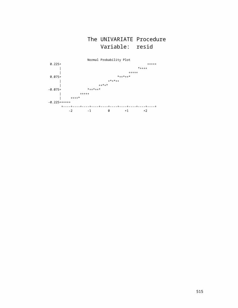
For Block X Factor A, the subscript is jk:
Type: R F R Rb fA n m
Effect j k i l SymbolBLKj 0 fA n m 2
BLKAk b 0 n m 2
TRBLK X Ajk 1 0 n m 2
TRBLKi(jk) 1 1 1 m 2
EEl(ijk) 1 1 1 1
For Block by Factor A, the E[MSBLK X TR] is:
515

For the experimental units nested in blocks by treatments, the subscript is ijk:
Type: R F R Rb fA n m
Effect j k i l SymbolBLKj 0 fA n m 2
BLKAk b 0 n m 2
TRBLK X Ajk 1 0 n m 2
TRBLKi(jk) 1 1 1 m 2
EEl(ijk) 1 1 1 1
For the experimental units, the E[MSEE] is: 22
SEEEm And for the samples in each experimental unit, the E[MSSE] is:
2SE
516

Power of the Test
Four possible results from Hypothesis testing:Reject H0 Accept H0
H0 True 1-H0 False 1-
1. H0 is true, and we accept H0 (we fail to reject it). Correct outcome. Probability of this is 1-
2. H0 is false (H1 is true instead) and we reject H0. Correct outcome. Probability of this is 1-This is called the Power of the Test.
3. H0 is true, but we reject H0. Not correct! Called the Type I error rate, the chance of rejecting a null hypothesis when it is true. For example, you reject when the means are actually the same, for a fixed-effects factor The probability of this happening is α, the significance level that you select.
4. H0 is false, but we accept H0 (we fail to reject it). Not correct! Called the Type II error rate, with a probability of β , the chance of accepting a null hypothesis when it is false. For example, you fail to reject H0: when the underlying population means are actually different.
517

Let’s say we are looking at a simple hypothesis, that the true mean is equal to a value, 0:
H0: 0
We then test this by: Collecting a number of observations (n) from the
population with mean of Calculating the sample mean, y is an unbiased estimate
of If we repeat this a number of times, the sample means
will vary around the real mean, with some sample means being far away from
The variance of the sample means among different sample sets will depend upon:o The number of observations in each sample set: As
n , the variance of these means will decrease.o If the variance in the observations is low, the
variance of these means will also be low, for a given n.
518

Let’s say the alternative is that the true mean is greater than 0:
H1:0
and state this as:
H1 1 where this is larger than 0.
Using a t-test (the y values follow a normal distribution, or n is large), sometimes we will reject H0: 0, even when the sample was from that population.
is the significance level that we set.
is the probability that we reject H0 when it is true, a Type I error, and conclude that it came from the population with 1. An error!
-3.5 -2.5 -1.5 -0.5 0.5 1.5 2.5 3.5 0
519

We choose but how do we get
= Type II error; is the probability that we Accept H0 (do not reject) when it is false,
e.g., if is really equal to 1 . The Power of the Test is 1-
is directly related to the level that we chose.If we set smaller (Type I error), will get larger (Type II error)!
Examples: 1. sample mean = -2.5. Conclusion?
2. sample mean =0.5. Conclusion? Correct? Depends!
3. sample mean=2.5. Conclusion? Correct? Depends!
4. sample mean =4.5. Conclusion? Correct?
-3.5 -2.5 -1.5 -0.5 0.5 1.5 2.5 3.5 4.5 5.5
0 1
520

How do we increase Power of the Test?
1. If we set larger, will get smaller. But then the Type I error is larger!
“lumpers” – large “splitters” – small 2. If 1 is very far from 0, will get smaller.
As our alternative hypothesis (e.g., 1) moves farther away from the null value (e.g., 0),
decreases and the power of the test increases.
3. Reduce the variance of the sample mean between different sample sets by:
o number of observations in each sample: As n , the variance of these means will decrease.
o If the variance in the observations is low, the variance of these means will also be low, for a given n. Can do this via stratifying, or in experiments, by blocking.
-3.5 -2.5 -1.5 -0.5 0.5 1.5 2.5 3.5 4.5 5.5 0 1
521

For experiments, for a given level, power changes with:
the sizes of the real differences between true
(population) treatment means, and
variation between experimental unit means (the means
from the experiment) for a given treatment.
the type of test we use to test our hypothesis. For
experimental design, we use an F-test (or more than one
F-test)
CAUTION: If there are repeated measures, spatial
correlations, unequal variances, and/or non-normality
for the error term(s), this becomes very complex. Can
use transformations to meet the assumptions in some
cases.
522

In Power Analysis for experiments, we want to either:
1. Calculate the Type II error and the power after the experiment is done, given the size of differences that we had in our experimental data, OR
2. Calculate the Type II error before conducting the experiment putting in the size of the differences that we wish
to detect (e.g., how much more does height growth have to be before we would add fertilizer?)
the level, and change the experiment (more experimental units)
to achieve a certain power (e.g., 0.80)
If Power analysis is used to alter the experiment, prior to it being conducted, then any differences that are detected, WILL BE DIFFERENCES OF PRACTICAL IMPORTANCE.
523

How do we calculate Power after conducting the experiment ( post-hoc power analysis)? Steps:
1. The experimental design is already set, along with the number of experimental units in each treatment, and the sizes of differences that were detected in the experiment.
2. Choose e.g., 00
3. Find the critical region using
e.g., suppose we have a CRD: one fixed-effect factor, with:J=5 treatments, and df treatment is 5-1=4n=3 observations in each treatment, and df error is 5(3-1)=10Therefore, Fcritical is F(0.95,4,10)=3.48
0.0 1.0 2.0 3.0 4.0
F(4,10,0.95)
524

4. Power is the probability that we would get the Fcritical or a larger value, if H1 was true (the means differed by the amounts given in the experiment). Need to estimate the size of the treatment effects (differences between means and the grand mean) based on the experiment to get this probability.
E.g., for the example, the experimenter calculated: SSTR=753 so MSTR=753/(5-1)=188.25MSE=5.23 We know that E[MSTR ]=TR+
2 and E[MSE]= 2
, and that:
69.244)23.575.188(3
15ˆ
)(1ˆ
1][][
1][
1
1
2
1
2
221
2
21
2
1
2
J
jj
TR
J
jj
J
jj
TR
J
jj
TR
jj
J
jj
TR
MSEMSn
JJ
nMSEEMSEthen
J
nMSEso
whereJ
n
525

Power is then Prob(F>Fcritical | Noncentral) where Noncentral is the noncentrality parameter, when H1 is true. This is called a “Noncentral F-distribution”.
Using the treatment effects we did get in the experiment, we can then calculate the noncentrality parameter, and find this probability.
36.14023.5
69.2443ˆ
21
2
noncentral
nnoncentral
J
jj
for n=3.
Then use SAS:
Data power;* Power=1-probf(Fcritical,df Treatment, df Error, Noncentral);Power=1-probf(3.48,4,10,140.36);Run;The temporary file will have the result in it, which is 0.9999. Very high power. Often try to get power between 0.80 and 0.95.
0.0 1.0 2.0 3.0 4.0
F(4,10, 0.95)
1
526

How do we calculate Power before conducting the experiment? Steps:
1. Select the experimental design E.g., simplest is CRD with one fixed-effect factor. Power analysis changes with the design, since the numerator and the denominator of the F-tests change.
2. State each H0 and H1. BUT H1 must be explicit, as to the size of the differences that you wish to detect. E.g. CRD with one fixed-effect factor: H1: 1=10, 2=11, 3 = 12, 4 = 13, 5 = 14 With a grand mean of 12, so the treatment effects are 1=-2, 2=-1, 3=0, 4=+1, 5=+2, and:
101
2
J
jj
We would like to detect quite small differences. If we reject H0, and conclude H1, the differences are at least this large (called minimum distances). And if these differences are detected, this is a difference of practical importance.
3. Choose e.g., 00Find the critical F value using e.g, for 3 experimental units per treatment, df(error) is 5(3-1)=10. F(4, 10, 0.95) = 3.48. Therefore, the critical region is F>3.48
527

4. Power is the probability that we will get Fcalculated that is greater than 3.48, given that the means are as given in H1 (i.e. H1 is true). We again need use the noncentral F distribution:
Power=Prob(F>Fcritical | Noncentral) where Noncentral is the noncentrality parameter, when H1 is true. Using the treatment effects we wish to be able to detect (or larger differences), we can then calculate the noncentrality parameter, and find this probability. BUT we need an estimate of the variance of the error terms from a previous similar experiment!
Using the last experiment as being similar: MSE=5.23 is our estimate of the variance of the errors.
74.523.5103ˆ
21
2
J
jjn
noncentral
for n=3.
Then use SAS:Data power;* Power=1-probf(Fcritical,df Treatment, df Error, Noncentral);Power=1-probf(3.48,4,10,140.36);Run;
The temporary file “power” will have the result in it, which is 0.30. Very low power. Often try to get power between 0.80 and 0.95. These are small differences which will be harder to detect.
528

Options:
1. What about increasing this to n=4 experimental units per treatment (20 experimental units for the experiment)? The df treatment is still 4, but the df(error) is J(n-1) which is 5(4-1)=15. This has a critical F(4,15,0.95)= 3.06
65.723.5104ˆ
21
2
J
jjn
noncentral
for n=4.
Data power;* Power=1-probf(Fcritical,df Treatment, df Error, Noncentral);Power=1-probf(3.06,4,15,7.65);Run;
This results in a power of 0.44. The chance of rejecting H0 when there is at least these differences is only 44%. There is a large chance of accepting H0, when it is false (Type II error).
529
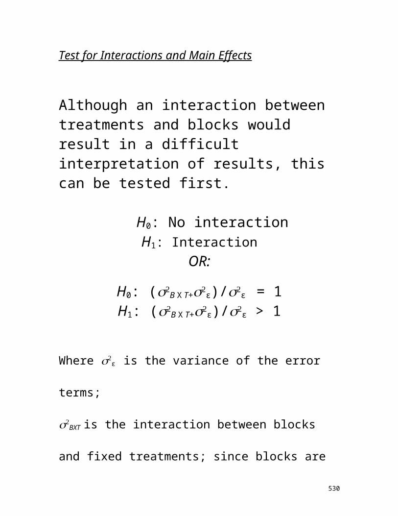
2. Another option is to use a different experimental design. What if we think we can reduce the MSE to 1.5 by using 2 Blocks in the design, but only n=2 experimental units per treatment (5 X 2 X 2=20 experimental units in total). We then have J=2 blocks, K=5 treatments, and n=2 experimental unit in each Block/Treatment combination. The df(error) is then JK(n-1) which is 2 X 5 (2-1)=10. The F critical is F(4,10,0.95)=3.48.
3.135.1102ˆ
21
2
J
jjn
noncentral
Data power;* Power=1-probf(Fcritical,df Treatment, df Error, Noncentral);Power=1-probf(3.48,4,10,13.3);Run;
The power is now 0.63.
530

3. Power is still not high enough, but cannot afford more experimental units or blocks? Change your expectations, also:
H1: 1=9, 2=11, 3 = 12, 4 = 13, 5 =15 With a grand mean of 12, so the treatment effects are
1=-3, 2=-1, 3=0, 4=+1, 5=+3, and: 201
2
J
jj
The F critical is F(4,10,0.95)=3.48, as in option 2.
7.265.1202ˆ
21
2
J
jjn
noncentral
For n=2 and using the estimated variance of the error terms when 2 blocks are used.
Data power;* Power=1-probf(Fcritical,df Treatment, df Error, Noncentral);Power=1-probf(3.48,4,10,26.7);Run;
The power is now 0.92! Only an 8% chance of a Type II error.
See SAS code called One_way_anova_power_using_min_differences.sasGives power for different alpha levels, and n.
References:
531

Textbook: [newest edition in White]Ch. 16.10; 19.11; 21.9;
Biometrics Information Handbook and Pamphlets (see www.forestry.ubc.ca/biometrics and click on “link” to find the website for these handbooks), particularly:
Nemec, A.F. 1991. Power analysis handbook for the design and analysis of forestry trials, Handbook No. 2. BC Ministry of Forests, Research Branch, Victoria, BC.
Bergerud, W. 1995. Post-hoc power analyses for ANOVA F-tests. Pamphlet #52. BC Ministry of Forests, Research Branch, Victoria, BC.
Bergerud, W. 1992. A general description of hypothesis testing and power analysis. Pamphlet #37. BC Ministry of Forests, Research Branch, Victoria, BC.
Bergerud, W.1995. Power analysis and sample sizes for completely randomized designs with subsampling. Pamphlet #49. BC Ministry of Forests, Research Branch, Victoria, BC.
Bergerud, W.1995. Power analysis and sample sizes for randomized block designs with subsampling. Pamphlet #50. BC Ministry of Forests, Research Branch, Victoria, BC.
Bergerud, W.1995. Programs for power analysis/sample size calculations for CR and RB designs with subsampling. Pamphlet #51. BC Ministry of Forests, Research Branch, Victoria, BC.
532

Example from Nemec, A.F. 1991. Power analysis handbook for the design and
analysis of forestry trials, Handbook No. 2. BC Ministry of Forests, Research Branch, Victoria, BC.
Pp 15-16.1. Experiment:
J=5 treatments, and df treatment is 5-1=4n=3 observations in each treatment, and df error is 5(3-1)=10
Therefore, Fcritical is F(0.90,4,10)=2.6052. Set means for H1:
H1: 1=600, 2=500, 3 = 500, 4 = 400, 5 =400 With a grand mean of 480, so the treatment effects are
1=120, 2=20, 3=20, 4=-80, 5=-80, and: 000,281
2
J
jj
3. Estimate standard deviation of the errors as 200 cm, so variance of the errors is 2002.4. Calculate noncentrality parameter:
1.2000,40
000,283ˆ2
1
2
J
jjn
noncentral
For n=3.
533

4. Calculate power using SAS:
Data power;* Power=1-probf(Fcritical,df Treatment, df Error, Noncentral);Power=1-probf(2.605,4,10,2.1);Run;
The power is 0.224.
534
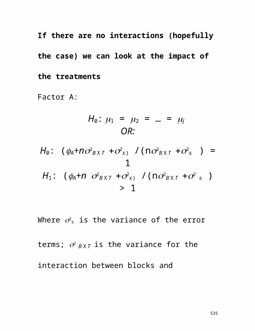
Use of Linear Mixed Models for Experimental Design
What are linear mixed models?
They are a group of linear models that include: One dependent variable , that is continuous (usually
labeled as Y or y in textbooks) fixed components
o continuous variables, and/or class variables represented by dummy (indicator) variables;
o fixed-effects in experimental design, predictor variables in regression, usually labeled as X or x;
o associated coefficients are labeled as β in most texts. error term
o usually labeled as (use e if this is estimated errors, not population errors)
o covariance matrix: variances and covariances of the errors; labeled the R matrix in many mixed models text books
o error terms follow a normal distributiono error terms may have unequal variance, and /or
correlations (time and/or space) between error termso error terms are a random component.
535

and may include, also: random components
o covariance matrix (variances and covariances of these random components) is labeled the G matrix in many texts
o the “variables” (really a design matrix) are labeled as Z, with associated coefficients “u”.
o these also follow a normal distributiono some models have only random components, and no
fixed components
Aside: In math symbols, this becomes:
RZGG'V(y)εuZβxy Estimates of all parameters:
o the fixed component coefficients (including the intercept),
o the variances for: the random components variances and
covariances; and random-effects coefficients variances (and covariances) of the error term
are estimated using maximum likelihood
536

Likelihood
Given a set of the estimated parameters (coefficients and variances/covariances), what is the chance that we would get the data that we did get?
For a discrete distribution of y (not the case in linear mixed models), this would be a probability for the first observation X the prob of the second observation, etc. to the last observation – between 0 and 1.
For a continuous distribution, e.g., normal, this is the value of the probability density function for the first observation X the probability density function for the second observation, etc to the last observation – not necessarily less than 1.
Maximum Likelihood
Change the set of estimated parameters until we get the largest possible likelihood.
Often easier to take the logarithm of the likelihood to do this – most packages report the log likelihood, or -2 X log likelihood.
537

Searching for the Maximum Likelihood
Most packages get the maximum likelihood by:o Searching for a set of all of these estimated
parameters that will result in the maximum likelihood of obtaining the data that we did get (ML method)
ORo Finding estimates of the fixed component coefficients
first (sometimes using least squares methods), and then using the residuals from that to get the random components (REML).
Because this is a search to find a solution (the estimates that give the maximum likelihood), the search proceeds by :
o getting estimates, calculating the (log) maximum likelihood (one iteration),
o altering the estimates, and recalculating the maximum likelihood (another iteration), and
o so on, until the estimates don’t change (or this may stop based on the likelihood does not change.
538

However, the search may not converge – o means that the estimates are not becoming the same
over the iterations of the search. o You may need to:
increase the number of iterations, change the way the search is done (e.g.,
Marquardt is one method for searching that is commonly used)
It may mean that your model is not correctly specified, or it is just very hard to find a solution if your models if very complex.
The search may converge, but with the statement that the “Hessian is not positive definite”
o This will mean that the variance estimates are not reliable.
o This can occur with a complex model, or when the model is not correctly specified.
539

Mixed models for experimental design
Linear mixed models enable us to get estimates for mixed-effects models, including: testing the fixed-effects factors for interactions, and main
effects (Type III SS, F-tests). SAS will use the correct F-tests based on Expected Means Squares.
Get t-tests for pairs of means using the correct denominator Mean Squares (same as the one used in the F-test)
Get estimates of the variances for the random effects, including the variance of the residual error.
Testing assumptions: bit harder to do!o Use residuals from GLM and do the tests?o Check the log likelihood – should be better (higher
log likelihood OR lower -2 log L) as you better meet the assumptions.
Example 1: CRD with one-fixed and one-random factor (handed out in class) -- discussion.
Others used in class: Time permitting only. Example 2: Randomized Block Design with replicates in each block (Generalized Block Design; handed out in class as one of the designs under Randomized Block Design with other Experiments)
Example 3: CRD: one fixed-effect factor with subsampling
540

References:Littell, R.C., G. A. Milliken, W.W. Stroup, and R.D. Wolfinger. 1996. SAS system for Mixed Models. SAS Institute Inc., Cary, NC.
Pineiro, J.C. and D.M. Bates. 2000. Mixed-effects models in S and S-plus. Springer, New York.
Schabenberger, O. and F. J. Pierce. 2002. Contemporary Statistical Models. CRC Press, New York (available electronically to UBC students as by accessing:
1. www.library.ubc.ca 2. Indexes and Databases3. Stats Net Base4. Then search for “Schabenberger”5. Then select Chapter 7. “Linear mixed models for
clustered data.”
NOTES:
1. Generalized Linear Mixed Models allow for class variables and count variables also (PROC GLMMIX).
2. Nonlinear Mixed Models allow for nonlinear models (PROC NLMIX).
541

CRD: Random and Mixed Effects
Example Using SAS: Two Factors, CRD.
Factor A, (three levels of fertilization: A1, A2, and A3) (J=3)
– fixed-effects
Factor B (four species: B1, B2, B3 and B4) (K=4) Random-
effects
Crossed: 12 treatments
Four replications per treatment (n=4) for a total of 48
experimental units
Measured Responses: height growth in mm
species is random -- these are a few of the species that we are
interested in and we wish to look at the variance in height
growth that is due to species.
542

Expected Mean Square Values Comparison:
Mean
Square
Model I
Both A and
B are Fixed
Model II
Both A and B are
Random
Model III
A is Fixed
B is Random
A
(MSA)A
2* 222
ABA nnK 22
ABA n
B
(MSB)B
2 222
ABB nnJ 22
BnJ
A X B
(MSAB)AB
2 22
ABn 22
ABn
Error
(MSE)
2
2
2
543
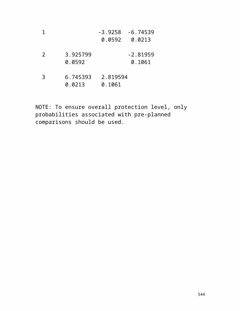
SAS CODE:
PROC IMPORT OUT= WORK.twofactor DATAFILE= "E:\frst430\lemay\examples\encyl_examples.xls" DBMS=EXCEL REPLACE; SHEET="crd$"; GETNAMES=YES; MIXED=NO; SCANTEXT=YES; USEDATE=YES; SCANTIME=YES;RUN;
options ls=70 ps=50 pageno=1;
* Using the same data as for fixed two-factor experiment, but assuming that factor b is random;PROC GLM data=twofactor;class a b;model result=a b a*b;random b a*b/test;test h=a e=a*b;lsmeans a /e=a*b pdiff tdiff;output out=glmout r=resid p=predict;run;
proc plot data=glmout;plot resid*predict='*';run;
proc univariate data=glmout normal plot;var resid;run;
PROC MIXED data=twofactor;class a b;model result=a;lsmeans a/pdiff;random b a*b;run;
544

The SAS System 1
The GLM Procedure
Class Level Information
Class Levels Values
A 3 1 2 3 B 4 1 2 3 4
Number of Observations Read 48 Number of Observations Used 48 The SAS System 2
The GLM Procedure
Dependent Variable: result result
Sum ofSource DF Squares Mean Square F Value
Model 11 2209.916667 200.901515 164.37Error 36 44.000000 1.222222Corrected Total 47 2253.916667
Source Pr > F
Model <.0001 Error Corrected Total
R-Square Coeff Var Root MSE result Mean
0.980478 4.850640 1.105542 22.79167
545

Removed Type I SAS output.
Source DF Type III SS Mean Square F Value
A 2 1258.166667 629.083333 514.70B 3 934.750000 311.583333 254.93A*B 6 17.000000 2.833333 2.32
Source Pr > F
A <.0001 B <.0001 A*B 0.0539
The SAS System 4
The GLM Procedure
Source Type III Expected Mean Square
A Var(Error) + 4 Var(A*B) + Q(A)B Var(Error) + 4 Var(A*B) + 12 Var(B) ????A*B Var(Error) + 4 Var(A*B) These are not reliable – do not match textbooks nor determination of EMS using the rules. Tests on the following page also not useful.
546

The SAS System 5
The GLM Procedure
Tests of Hypotheses for Mixed Model Analysis of Variance
Dependent Variable: result result
Source DF Type III SS Mean Square F Value
* A 2 1258.166667 629.083333 514.70 B 3 934.750000 311.583333 254.93 A*B 6 17.000000 2.833333 2.32
Error: MS(Error) 36 44.000000 1.222222 * This test assumes one or more other fixed effects are zero.
Source Pr > F
* A <.0001 B <.0001 A*B 0.0539
Error: MS(Error)* This test assumes one or more other fixed effects are zero.
547

The SAS System 6
Least Squares Means Standard Errors and Probabilities Calculated Using the Type III MS for A*B as an Error Term
result LSMEAN A LSMEAN Number 1 16.2500000 1 2 23.3750000 2 3 28.7500000 3
Least Squares Means for Effect A t for H0: LSMean(i)=LSMean(j) / Pr > |t|
Dependent Variable: result
i/j 1 2 3
1 -11.9724 -21.0042 <.0001 <.00012 11.97239 -9.03181 <.0001 0.00013 21.0042 9.031807 <.0001 0.0001
NOTE: To ensure overall protection level, only probabilities associated with pre-planned comparisons should be used.MUST use the Bonferroni correction. For every test, compare the p-value to alpha/# pairs.
548

The SAS System 7
Dependent Variable: result result
Tests of Hypotheses Using the Type III MS for A*B as an Error Term
Source DF Type III SS Mean Square F ValueA 2 1258.166667 629.083333 222.03
Source Pr > F
A <.0001
From class, we estimated the variance for Factor B as (n=
86.2534
22.158.311ˆ
][][][][
][
][
2
2
2
2
22
2
2
nJMSEMSBnJ
MSEEMSBEnJMSEEMSBE
MSEE
nJMSBE
B
B
B
B
549

The SAS System 8
Plot of resid*predict. Symbol used is '*'.
resid ‚ ‚ 2.50 ˆ * 2.25 ˆ 2.00 ˆ 1.75 ˆ * 1.50 ˆ * 1.25 ˆ * * * * * 1.00 ˆ * 0.75 ˆ * * 0.50 ˆ * * 0.25 ˆ * * * * * 0.00 ˆ * *-0.25 ˆ * * *-0.50 ˆ * *-0.75 ˆ * * * * *-1.00 ˆ *-1.25 ˆ * * *-1.50 ˆ *-1.75 ˆ-2.00 ˆ-2.25 ˆ-2.50 ˆ * ‚ Š-ˆ---------ˆ---------ˆ---------ˆ---------ˆ---------ˆ---------ˆ- 10 15 20 25 30 35 40
predict
NOTE: 12 obs hidden.
Some SAS outputs removed. The SAS System 9
The UNIVARIATE Procedure Variable: resid
Tests for Normality
Test --Statistic-- --p Value----
Shapiro-Wilk W 0.977162 Pr < W 0.4666Kolmogorov-Smirnov D 0.114207 Pr > D 0.1169Cramer-von Mises W-Sq 0.082279 Pr >W-Sq 0.1963Anderson-Darling A-Sq 0.513709 Pr >A-Sq 0.1926
550

The SAS System 11
The UNIVARIATE Procedure Variable: resid
Stem Leaf # Boxplot 2 5 1 | 2 | 1 58 2 | 1 022222 6 | 0 558888 6 +-----+ 0 00000022222 11 *--+--* -0 2222 4 | | -0 888888888855 12 +-----+ -1 2220 4 | -1 5 1 | -2 | -2 5 1 | ----+----+----+----+
Normal Probability Plot 2.75+ * | +++++ | *+*++ | ***+**+ | **+*++ | *****+* | +***+ | **+**+** | * *++*++ | +++++ |+++*+ -2.75+ +----+----+----+----+----+----+----+----+----+----+ -2 -1 0 +1 +2
551

The SAS System 12
The Mixed Procedure
Model Information
Data Set WORK.TWOFACTOR Dependent Variable result Covariance Structure Variance Components Estimation Method REML Residual Variance Method Profile Fixed Effects SE Method Model-Based Degrees of Freedom Method Containment
Class Level Information
Class Levels Values A 3 1 2 3 B 4 1 2 3 4 Levels for A and B correct. Dimensions Covariance Parameters 3 Columns in X 4 Columns in Z 16 Subjects 1 Max Obs Per Subject 48Have 3 covariance parameters, as there are 3 random components: B, A X B, and the error term. Columns in X: 4. Why? Factor A uses 3 dummy variables for 3 levels, plus the intercept. (NOTE: can use “noint” – to remove the intercept)Columns in Z: 16. Why?
Factor B has 4 levels. Uses 4 dummy variables Factor A X B is 3 dummy variables for Factor A X 4 dummy variables for Factor B= 12
Subjects: only one dataset – not subdivided by anything. So 48 obs in one subject (n=4 exp. units per treatment)
552

Number of Observations
Number of Observations Read 48 Number of Observations Used 48 Number of Observations Not Used 0
Iteration History
Iteration Evaluations -2 Res Log Like Criterion
0 1 275.37975211 1 1 166.72010292 0.00000000
The SAS System 13
The Mixed Procedure Convergence criteria met.
Covariance Parameter Estimates
Cov Parm Estimate
B 25.7292 A*B 0.4028 Residual 1.2222
Fit Statistics
-2 Res Log Likelihood 166.7 AIC (smaller is better) 172.7 AICC (smaller is better) 173.3 BIC (smaller is better) 170.9Instead of R Squared used in least squares, we have -2 Res (residual) log likelihood. Instead of R squared adjusted, we have AIC, AICC, BIC
553

Type 3 Tests of Fixed Effects
Num Den Effect DF DF F Value Pr > F
A 2 6 222.03 <.0001
Correct F-test. Least Squares Means
StandardEffect A Estimate Error DF t Value Pr>|t|A 1 16.2500 2.5709 6 6.32 0.0007A 2 23.3750 2.5709 6 9.09 <.0001A 3 28.7500 2.5709 6 11.18 <.0001
df(MSAB)=(3-1)X(4-1)=6
From the GLM output, we expected:
KnMSABmeanlevelAFactorES )(.
For mixed models, MSAB is replaced with:
)4028.0)(4(22.1ˆˆ2
ABnMSAB =2.8312
[was 2.833 using least squares)
4207.044
833.2)(.
meansAFactorES
WHY is this given as 2.5709?? VERY different using PROC MIXED vs PROC GLM. Why?
554

Littell and others (1996) indicate that the ones in GLM are not correct. That we should add in all of the random variances.
Using the population model for two factors:Population:
They suggest that for the Factor A level means are calculated as:
jjABBjAjy
When Factor B is fixed, the effects due to B and AB do not contribute to the variance (the average effect for B is 0, as well as the other terms). Then the variance of the Factor A level means is simply the variance of the error term (estimated by MSE), divided by the number of observations for that Factor A level (and the F-test is MSA/MSE).
When Factor B is random, the F-test is MSA/MSAB, to isolate the effects for Factor A.
555

For confidence intervals on Factor A level means, there is the variance of the error term + variance of B + variance of AB divided by the number of observations in this Factor A level. This means the standard error would be changed to:
Knnn
KnKK
raVraVraV
ABBABB
jjABB
22
ˆˆˆˆˆˆ
)(ˆ)(ˆ)(ˆmeans) levelA (Factor Variance Estimated
2222
Divisors: K values used to calculate the average Factor B effect;
K values used to calculate the average interaction effect for each Factor A level;
Kn values used to calculate the average error for each Factor A level.
556

Standard Error (Factor A level means) is the square root of this. For the example:
5723.244
76.25)4(4028.0)4(22.1
As per the MIXED output [shows 2.5709]
Differences of Least Squares Means
StandardEffect A A Estimate Error DF t Value Pr>|t|
A 1 2 -7.1250 0.5951 6 -11.97 <.0001A 1 3 -12.5000 0.5951 6 -21.00 <.0001A 2 3 -5.3750 0.5951 6 -9.03 0.0001
Pairs of means t-tests same as for GLM using A X B as the error term for Factor A.
5949.044
144
18312.2
21
11)21(.
XX
nobsnobsMSABmeanmeanES
Corresponds with least squares means, as other variance terms cancel out when we get the variance in the difference of the means.
557

Randomized Block Design with replicates in each block
Example: Randomized Block Design (RCB), with Factor A (three types of food: A1 to A3), and two labs (blocks). Randomization of Factor A is restricted to within labs.
Lab 1 Lab 2
A1 = 6 A1=5 A3=11 A3=12
A3=10 A2=8 A1=4 A2=9
A2=7 A3=12 A2=8 A1=5
Response variable: weight gain of fish (kg)Experimental unit: one tank of fish; 6 tanks in each lab
Use the SAME analysis as for CRD with one fixed and one
random factor – no difference in analysis. However, the
conclusions WILL vary, as we are only interested in sites as a
way to remove variation for the F-test, and for pairs of means t-
tests.
558

CRD: One Factor Experiment, Fixed Effects with
subsampling [26.7 of textbook (White)]
Example from Textbook: Have three temperatures: low, medium, and high For each, we have two experimental units (batches) For each batch, we have three loaves of bread The response variable is crustiness of bread.
Data:
temp batch observation yijllow 1 1 4low 1 2 7low 1 3 5low 2 1 12low 2 2 8low 2 3 10medium 1 1 14medium 1 2 13medium 1 3 11medium 2 1 9medium 2 2 10medium 2 3 12high 1 1 14high 1 2 17high 1 3 15high 2 1 16high 2 2 19high 2 3 18
SAS code: Three options presented
559

4. Using PROC GLM and the sample observations. Model yijk= treat batch(treat);
5. Using PROC MIXED, and the sample observations.Model yijk=treat; Random batch(treat);
The F-test for the treatment is F=MSTR/MSEE
For the mean of the treatment:
jSUjEUTRjjy
Where experimental errors are random, and the sampling errors are random, with a fixed treatment.
nmm
nmn
VarVar
SEEESEEE
jSUjEU
22 22
)()(means) levelA (Factor Variance Estimated
Since the numerator is the Expected value for MSEE , the standard error of the mean is estimated by:
nmMSmeanlevelAFactorES EE)(.
Get the same results using GLM as using MIXED. [also get the same results using the mean values for each experimental unit as the y-variable]
560

PROC IMPORT OUT= WORK.onesub DATAFILE= "E:\frst430\lemay\examples\ subsampling_neter_newest_p1109.xls" DBMS=EXCEL REPLACE; SHEET="data$"; GETNAMES=YES; MIXED=NO; SCANTEXT=YES; USEDATE=YES; SCANTIME=YES; RUN;
options ls=70 ps=50 pageno=1;
* Analysis 1. first, use GLM and bring in the Experimental error and the Sampling error into the design;PROC GLM data=onesub;class temp batch;model yijl=temp batch(temp);random batch(temp)/test;test h=temp e=batch(temp);lsmeans temp /e=batch(temp) pdiff tdiff;output out=glmout r=resid p=predict;run;proc plot data=glmout;plot resid*predict='*';run;proc univariate data=glmout normal plot;var resid;run;
* Analysis 2: this is using maximum likelihood for a mixed model to estimate variances and get correct F-tests;
PROC MIXED data=onesub;class temp batch;model yijl=temp;lsmeans temp/pdiff;random batch(temp);run;
561

Analysis 1: GLM using samples with experimental error given as batch(treat), and sampling error as the Error term. The SAS System 1
The GLM Procedure
Class Level Information
Class Levels Values temp 3 high low medium batch 2 1 2
Number of Observations Read 18 Number of Observations Used 18 The SAS System
The GLM Procedure
Dependent Variable: yijl yijl
Sum ofSource DF Squares Mean Square F Value
Model 5 284.4444444 56.8888889 21.79Error 12 31.3333333 2.6111111Corrected Total 17 315.7777778
Source Pr > F Model <.0001 Error Corrected Total
R-Square Coeff Var Root MSE yijl Mean
0.900774 13.59163 1.615893 11.88889
562

(NOTE: Type I SS removed)
Source DF Type III SS Mean Square F Valuetemp 2 235.4444444 117.7222222 45.09batch(temp) 3 49.0000000 16.3333333 6.26
Source Pr > F temp <.0001 batch(temp) 0.0084 NOTE: Variance components and GLM Mixed model analysis given by SAS removed – often not correct.
Least Squares MeansStandard Errors and Probabilities Calculated Using the Type III MS for batch(temp) as an Error Term
LSMEANtemp yijl LSMEAN Numberhigh 16.5000000 1low 7.6666667 2medium 11.5000000 3
Least Squares Means for Effect temp t for H0: LSMean(i)=LSMean(j) / Pr > |t|
Dependent Variable: yijl
i/j 1 2 31 3.785714 2.142857 0.0323 0.12152 -3.78571 -1.64286 0.0323 0.19903 -2.14286 1.642857 0.1215 0.1990
NOTE: To ensure overall protection level, only probabilities associated with pre-planned comparisons should be used.
563

Dependent Variable: yijl yijl
Tests of Hypotheses Using the Type III MS for batch(temp) as an Error Term
Source DF Type III SS Mean Square F Valuetemp 2 235.4444444 117.7222222 7.21
Source Pr > F temp 0.0715
Plot of resid*predict. Symbol used is '*'. resid ‚ 2.000 ˆ * ‚ ‚ 1.667 ˆ * * * ‚ ‚ 1.333 ˆ * * ‚ ‚ 1.000 ˆ ‚ ‚ 0.667 ˆ ‚ ‚ 0.333 ˆ * * ‚ ‚ 0.000 ˆ * ‚ ‚-0.333 ˆ * * * ‚ ‚-0.667 ˆ ‚ ‚-1.000 ˆ ‚ ‚-1.333 ˆ * * * ‚ ‚-1.667 ˆ * * ‚ ‚-2.000 ˆ * ‚ Šˆ---------ˆ---------ˆ---------ˆ---------ˆ---------ˆ---------ˆ- 5.0 7.5 10.0 12.5 15.0 17.5 20.0
predict
564

The UNIVARIATE Procedure Variable: residNOTE: All outputs removed except for Normality tests and box plot and normality plot
Tests for Normality
Test --Statistic--- -p Value------
Shapiro-Wilk W 0.908031 Pr<W 0.0794Kolmogorov-Smirnov D 0.17031 Pr>D >0.1500Cramer-von Mises W-Sq 0.084708 Pr>W-Sq 0.1732Anderson-Darling A-Sq 0.605378 Pr>A-Sq 0.0984
Stem Leaf # Boxplot 2 0 1 | 1 777 3 | 1 33 2 +-----+ 0 | | 0 033 3 | + | -0 333 3 *-----* -0 | | -1 333 3 +-----+ -1 77 2 | -2 0 1 | ----+----+----+----+
The UNIVARIATE Procedure Variable: resid
Normal Probability Plot 2.25+ +++* | * *+*+ | * *++++ 0.75+ ++++ | +**+* | *+** -0.75+ ++++ | +++** * | * +*+* -2.25+ ++++ +----+----+----+----+----+----+----+----+----+----+ -2 -1 0 +1 +2
565

Analysis 2: MIXED using each sample unit value. The SAS System The Mixed Procedure
Model InformationData Set WORK.ONESUBDependent Variable yijlCovariance Structure Variance ComponentsEstimation Method REMLResidual Variance Method ProfileFixed Effects SE Method Model-BasedDegrees of Freedom Method Containment
Class Level Information Class Levels Values temp 3 high low medium batch 2 1 2
Dimensions Covariance Parameters 2 Columns in X 4 Columns in Z 6 Subjects 1 Max Obs Per Subject 18
Number of Observations Number of Observations Read 18 Number of Observations Used 18 Number of Observations Not Used 0
Iteration HistoryIteration Evaluations -2 Res Log Like Criterion0 1 73.11545106 1 1 67.84036856 0.00000000
566

Convergence criteria met.
Covariance Parameter Estimates Cov Parm Estimate batch(temp) 4.5741 Residual 2.6111
Fit Statistics -2 Res Log Likelihood 67.8 AIC (smaller is better) 71.8 AICC (smaller is better) 72.8 BIC (smaller is better) 71.4
Type 3 Tests of Fixed Effects Num DenEffect DF DF F Value Pr > Ftemp 2 3 7.21 0.0715 Least Squares Means
StandardEffect temp Estimate Error DF t Value Pr>|t|temp high 16.5000 1.6499 3 10.00 0.0021temp low 7.6667 1.6499 3 4.65 0.0188temp medium 11.5000 1.6499 3 6.97 0.0061 Differences of Least Squares Means
Std.Effect temp temp Estimate Error DF t Value Pr>|t|temp high low 8.8333 2.3333 3 3.79 0.0323temp high medium 5.0000 2.3333 3 2.14 0.1215temp low medium -3.8333 2.3333 3 -1.64 0.1990
567

Brief Summary of the Course
All linear models Regression analysis and analysis of variance (ANOVA) or
analysis of covariance (ANCOVA) for experiments. y – is a continuous variable; “dependent” variable in
regression; “response” variable in experiments
Regression (Fitting Equations):
Reason: Prediction of the dependent variable (y; hard to measure) from related variables (x’s; easy to measure). Started with only continuous x variables, and then added class variables as predictors.
Model: yi = 0 + 1 x1i + 2 x2i +...+m xmi +i
Used least squares regression to find estimated coefficients and standard errors of the coefficients
Used “hand calculations” for SLR only.
568

SAS:PROC REG data=yourdata; model y=X1 X2 X3; output out=out1 p=yhat1 r=resid1;run;*------------------------------------------;PROC PLOT DATA=out1; plot resid1*yhat1;run;*-----------------------------------------;PROC univariate data=out1 plot normal;Var resid1;Run;Process:
1. Collect data on y and x’s.2. Run a model.3. Check assumptions. If met, go to step 5.4. If not met, transform the x and go back to step 2. If this does
not work, try transforming the y and repeat step 2. 5. Goodness of fit measures: R2 (or r2) and root MSE (SEE).6. Use an F-test to see if the model is significant. Null
hypothesis: H0: 1 = 2 =3 = . . . =m =0 [all slopes are zero meaning no relationship with x’s]
7. If the regression is significant, test each predictor variable (in the presence of the other x-variables), using a t-test.
8. Can calculate confidence intervals for each coefficient, and for the predicted values (mean predicted value, new observation, OR mean of g new observations).
569
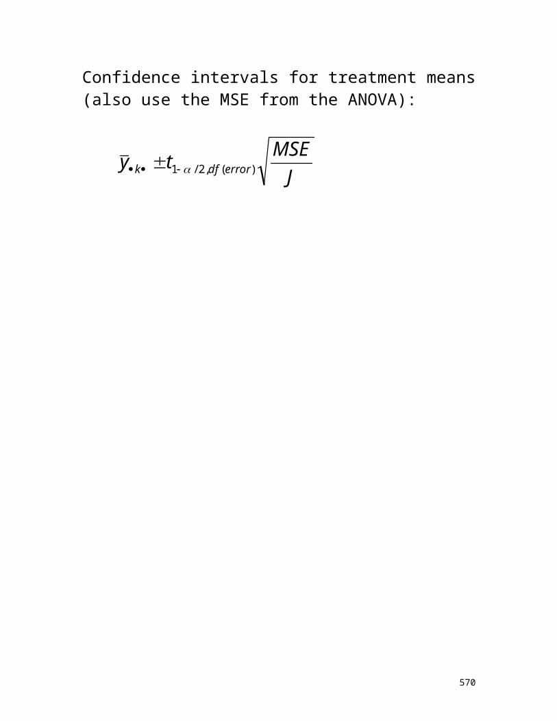
Adding class variables: Convert these to dummy variables. The set of dummy variables represents that class variable Dummy variables alter the intercept Interactions between dummy variables and the continuous
variables alter the slopes. Use a partial F-test as this can be used to test a group of
variables (the group of dummy variables, or the group of interactions between dummy variables and continuous variables), whereas a t-test is for a single variable (testing a single dummy variable has no meaning – the group of dummy variables represents that class; unless there is only two levels in the class, since this would be only 1 dummy variable)
Where r is the df(model) for the full model – df(model) for the reduced model.
Stepwise methods (as guides to selecting variables):1. All possible regressions2. R2 (or Adjusted R2). 3. Stepwise. 4. Backwards Stepwise5. Forward Stepwise 2m-1
CAUTION: Careful with dummy variables! Must come in or out of the model as a group, as the group represents one class variable.
570
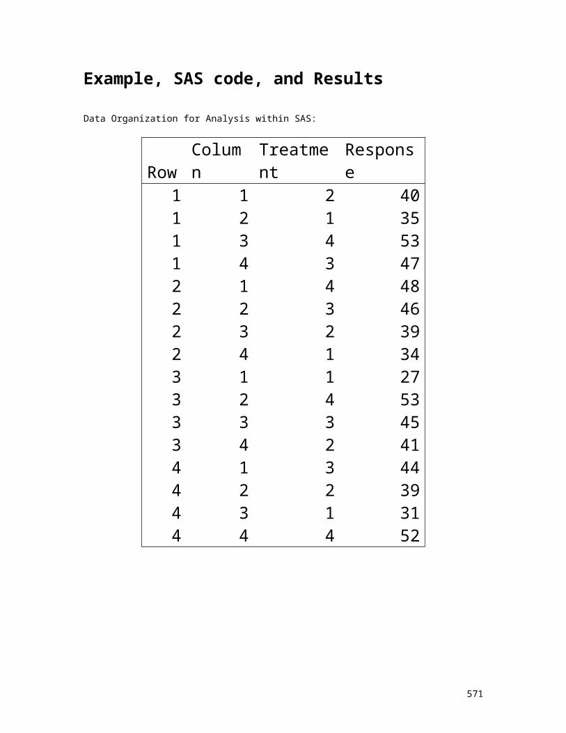
Experimental Design: Manipulate by using treatments We are interested in CAUSE and EFFECT NOTE: We did “hand” calculations for CRD, one-factor
only
Designs: Select homogeneous experimental units Randomly assign treatments to experimental units Treatments can be divided into Factors A crossed experiment (factorial) includes all combinations
of the factor levels from all Factor Factors can be nested in another factor – more difficult to
interpret and cannot look at interactions among factors Factors can be fixed-effect or random-effectNOTE: differences in the use of the word random:
o Random samplingo Random assignment of treatments to experimental
unitso Random-effects
Can “block” before assigning treatments to experimental units to reduce variability among experimental units
Can “split” experimental units for a second factor, or even split again “split-split plot for a third level – will affect the analysis and conclusions made
Can add “covariates” as measurements on continuous variables from each experimental unit, to reduce variability
Can have one measurement from each experimental unit (or an average for that unit), or can retain sampling unit measures but must divide the error in that case.
571
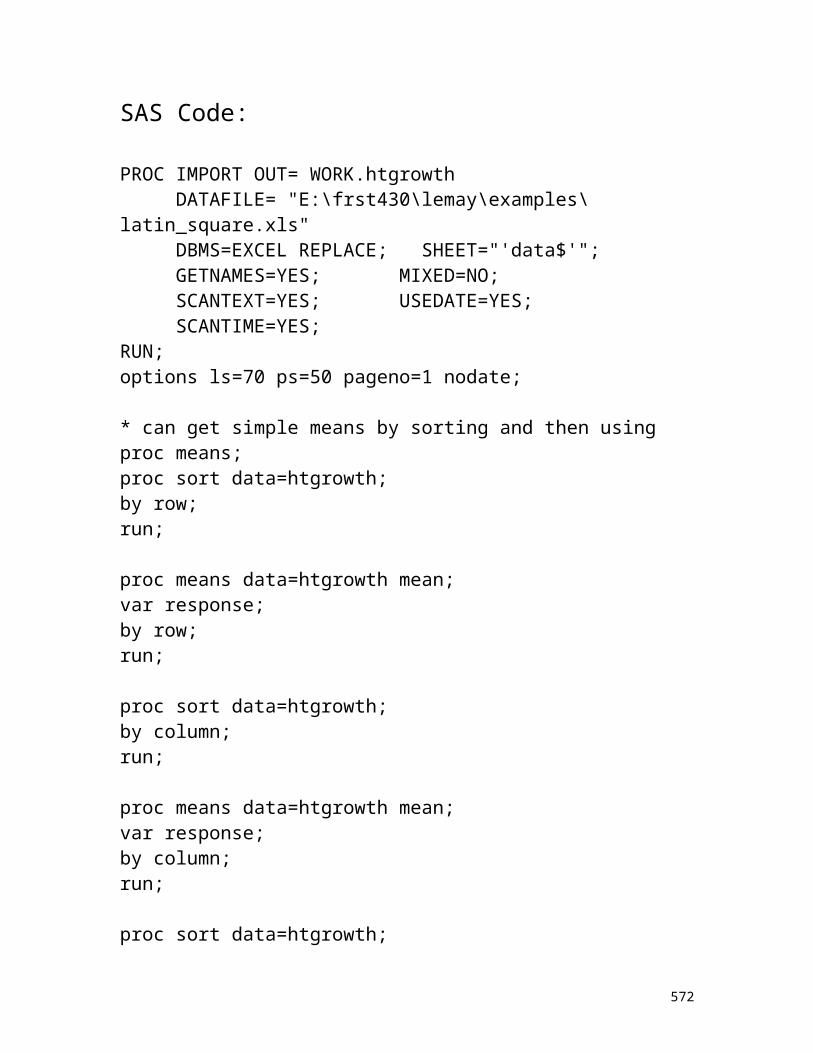
Error terms (experimental error and sampling error) are random-effects
Blocks are often random-effects F-tests are used to test for interactions (1st), and main effects. Expected means squares are used to determine which F-tests
to use to test each factor. If there is an interaction among factors, you cannot interpret
the main effects (each Factor) separately If there is a significant difference in means (for a main effect,
or there is an interaction), post comparison tests can be used to determine which means differ, IF the factor(s) are fixed-effects.
For random-effects factors (and interactions), we can use the MS’s to estimate the variance for that factor (or interaction)
572

Process for Analysis:1. Set up data in excel, by giving a label to each observation
as to which block, and factor levels it was measured for, experimental unit, sampling unit, etc.
2. Set up SAS (or other package) witha. the correct class statements, b. model statements, c. any necessary test statements (use the expected mean
squares to decide if the default is ok or not), and d. multiple comparisons (use LSMEANS for this in
SAS). e. Also, get a residual plot, normal probability plot, and
normality tests (for the residuals)3. Check the assumptions first. May have to transform the y-
variable until assumptions are met.4. When assumptions are met, use F-tests for interactions (if
any) first. Make sure you have the right F-test.5. If no interactions, check F-tests for main effects (e.g.,
Factor A, Factor B, etc).6. For fixed-effects (main or interactions) that show
significant differences among mean values, do pairs of means t-tests (or other multiple comparisons) to decide which means differ. Remember to divide alpha by the number of pairs of means when interpreting pairs of means t-tests.
7. For random-effects, estimate the variance for that factor. (can do this for error terms also as they are random-effects)
573

Models:
CRD with one factor: Model: SAS:PROC GLM data=yourdata;CLASS Treatment;MODEL y=treatment;MEANS treatment/scheffe hovtest=bartlett;estimate '1 VS others' treatment 4 -1 -1 -1 -1/divisor=4;OUTPUT OUT=GLMOUT PREDICTED=PREDICT RESIDUAL=RESID;RUN;PROC PLOT DATA=GLMOUT;PLOT RESID*PREDICT='*';RUN;PROC UNIVARIATE DATA=GLMOUT PLOT NORMAL;VAR RESID;RUN;
OR:Can use:MEANS treatment/pdiff tdiff hovest=bartlett;
Instead.
574

2-factor, CRD:Model:
SAS: both factors are fixed-effectsPROC GLM data=yourdata;class factorA factorB;model result=factorA factorB factorA*factorB;output out=glmout r=resid p=predict;lsmeans factorA factorB factorA*factorB/pdiff tdiff;run;proc plot data=glmout;plot resid*predict='*';run;PROC univariate data=glmout plot normal;Var resid;Run;
SAS: mixed-effects, A fixed-effect; B random-effectPROC GLM data=yourdata;class factorA factorB;model result= factorA factorB factorA*factorB;random factorB/test;test h= factorA e= factorA*factorB;lsmeans factorA/e= factorA* factorB pdiff tdiff;output out=glmout r=resid p=predict;run;proc plot data=glmout;plot resid*predict='*';run;proc univariate data=glmout normal plot;var resid;run;
575

RCB, one fixed-effectModel:
SAS:PROC GLM data=yourdata;class block treatment;model y=block treatment;random block;lsmeans treatment/pdiff tdiff;output out=glmout r=resid p=predict;run;[plus statements to obtain the residual plot and normality plot/tests]
RCB, two Factors: Model: SAS both Factors are fixed-effects, and blocks are random-effects:PROC GLM data=yourdata;class block factorA factorB;model y=block factorA factorB factorA* factorB;random block;lsmeans factorA/pdiff tdiff;lsmeans factorB/pdiff tdiff;lsmeans factorA* factorB/pdiff tdiff;output out=glmout r=resid p=predict;run;[plus statements to obtain the residual plot and normality plot/tests]
576

Generalized RCB, one Factor (RCB with replicates in each block)Model:
SAS (treatment is a fixed effect; blocks are random-effects)PROC GLM data=yourdata;class block treatment;model y=site treatment block*treatment;random block block*treatment;test h=treatment e=site*treatment;lsmeans treatment/e=site*treatment pdiff tdiff;output out=glmout r=resid p=predict;run;[plus statements to obtain the residual plot and normality plot/tests]
Latin Square, with blocking in two directionsOne fixed-effect factor:Model: SAS:PROC GLM data=yourdata;class row column treatment;model y=row column treatment;random row column;lsmeans treatment/pdiff tdiff;output out=glmout r=resid p=predict;run;[plus statements to obtain the residual plot and normality plot/tests]
577
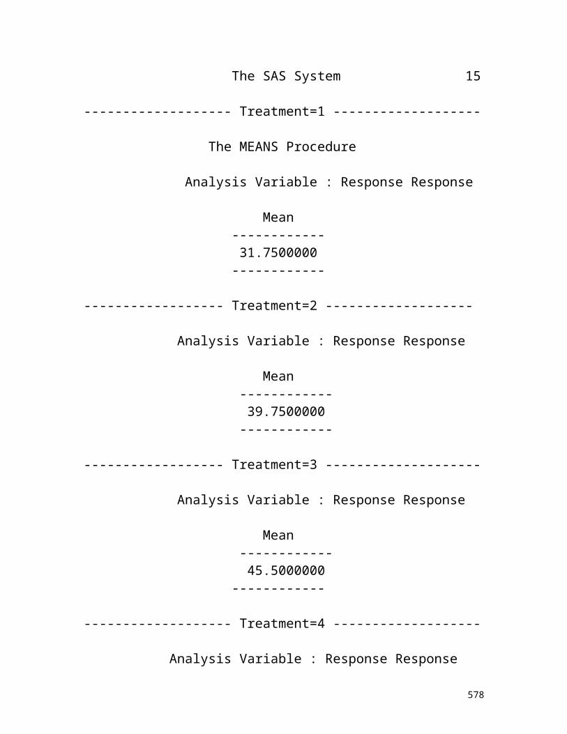
Split plots (and split-split plots):Model for a 2-factor RCB, split-plot:
SAS: blocks random-effects, Factor A fixed-effects, FactorB is applied to the split-plotPROC GLM data=yourdata;TITLE 'split plot, blocks random, treatments fixed';CLASS block factorA factorB;MODEL y=block factorA block*factorA factorB factorA*factorB;Test h=factorA e=factorA*block;LSMEANS factorA/e=block*factorA tdiff pdiff;LSMEANS factorB factorA*factorB/tdiff pdiff;OUTPUT OUT=GLMOUT PREDICTED=PREDICT RESIDUAL=RESID;RUN;[plus statements to obtain the residual plot and normality plot/tests]
Nested factors:For a crossed experiment (Factorial):
However, for a nested experiment, B nested in A, we have:Model: SAS:PROC GLM data=yourdata;class factorA factorA;model y= factorA factorB(factorA);output out=glmout r=resid p=predict;lsmeans factorA factorB(factorA)/pdiff tdiff;run;[plus statements to obtain the residual plot and normality plot/tests]
CRD: One Factor Experiment, Fixed Effects with subsampling
578

Model:
SAS: (note: expunitlabel is the label for the exp. units, eg., batch, board, etc)PROC GLM data=yourdata;class treatment expunitlabel;model y=treatment expunitlabel(treatment);random expunitlabel(treatment)/test;test h=treatment e= expunitlabel(treatment);lsmeans treatment /e= expunitlabel(treatment)pdiff tdiff;output out=glmout r=resid p=predict;run;[plus statements to obtain the residual plot and normality plot/tests]
NOTE: could instead average the sample values for each experimental unit, to obtain one value for that experimental unit, and analyze this as if there were no samples (error term is experimental unit).
Generalized RCB [randomized block design, also called randomized complete block] with subsampling:
Model:
[not given in class, but can modify the SAS code for generalized RCB]
579

Analysis of Covariance
Model: shown for CRD with two fixed-effect factors and one covariate; covariates are continuous variables; assuming no interactions between covariate and factors
SAS code [full model with interactions which are not shown in the model above, and reduce to only one factor]PROC GLM data=yourdata;CLASS factorA;Full: MODEL y=factorA x factorA*x/solution;OUTPUT OUT=GLMOUT2 PREDICTED=PREDICT2 RESIDUAL=RESID2;RUN;PROC PLOT DATA=GLMOUT2;PLOT RESID2*PREDICT2='*';RUN;PROC UNIVARIATE DATA=GLMOUT2 PLOT NORMAL;VAR RESID2;RUN;
Compare to the classical analysis of covariance model with no interaction between the covariates and the factors:PROC GLM data=yourdata;CLASS factorA;Full: MODEL y=factorA x/solution;OUTPUT OUT=GLMOUT3 PREDICTED=PREDICT3 RESIDUAL=RESID3;RUN;PROC PLOT DATA=GLMOUT3;PLOT RESID3*PREDICT3='*';RUN;PROC UNIVARIATE DATA=GLMOUT3 PLOT NORMAL;VAR RESID3;RUN;
Using a partial F-test:
580

SSreg=SSmodelr=df(model for full model)-df(model for reduced model)
df for numerator of F is rdf for denominator of F is df(error full model)
581

Expected Mean Squares: Given for all models covered Can calculate this using the “rules” for any model (not be
required to do this on an exam)
Power analysis:Four possible results from Hypothesis testing:
Reject H0 Accept H0H0 True 1-H0 False 1-
Set Type I error () Solve for Type II error (β) Power is 1- β
582