form approved report documentation page omb … · · 2014-09-18project number 5e. task number...

REPORT DOCUMENTATION PAGE Form Approved

OMB No. 0704-0188

The public reporting burden for this collection of information is estimated to average 1 hour per response, including the time for reviewing instructions, searching existing data sources, gathering and maintaining the data needed, and completing and reviewing the collection of information. Send comments regarding this burden estimate or any other aspect of this collection of information, including suggestions for reducing the burden, to Department of Defense, Washington Headquarters Services, Directorate for Information Operations and Reports (0704-0188), 1215 Jefferson Davis Highway, Suite 1204, Arlington, VA 22202-4302. Respondents should be aware that notwithstanding any other provision of law, no person shall be subject to any penalty for failing to comply with a collection of information if it does not display a currently valid OMB control number. PLEASE DO NOT RETURN YOUR FORM TO THE ABOVE ADDRESS. 1. REPORT DATE (DD-MM-YYYY)

12-06-2014 2. REPORT TYPE

Final 3. DATES COVERED (From - To) 26 Sept 2012 to 25 Sept 2013

4. TITLE AND SUBTITLE

Multi-scale Computational Electromagnetics for Phenomenology and Saliency Characterization in Remote Sensing

5a. CONTRACT NUMBER FA2386-12-1-4082

5b. GRANT NUMBER Grant AOARD-124082

5c. PROGRAM ELEMENT NUMBER 61102F

6. AUTHOR(S)

Prof Hean-Teik Chuah

5d. PROJECT NUMBER

5e. TASK NUMBER

5f. WORK UNIT NUMBER

7. PERFORMING ORGANIZATION NAME(S) AND ADDRESS(ES) Universiti Tunku Abdul Rahman No9, Jalan Bersatu 13/4, Petaling Jaya, Selangor Darul Ehsan 47500 Malaysia

8. PERFORMING ORGANIZATION REPORT NUMBER

N/A

9. SPONSORING/MONITORING AGENCY NAME(S) AND ADDRESS(ES)

AOARD UNIT 45002 APO AP 96338-5002

10. SPONSOR/MONITOR'S ACRONYM(S)

AFRL/AFOSR/IOA(AOARD)

11. SPONSOR/MONITOR'S REPORT NUMBER(S)

AOARD-124082

12. DISTRIBUTION/AVAILABILITY STATEMENT

Approved for public release. 13. SUPPLEMENTARY NOTES This research effort is continued for two more years. 14. ABSTRACT For earth observation, microwave remote sensing has been a useful technology that provides sensing capability of earth terrain with wide coverage. Images from satellite based Synthetic Aperture Radar (SAR) are acquired to provide ground information about various types of earth terrain sensed (such as vegetation, farm, urban area, sea ice and snow covered land, etc). In order to interpret these SAR images correctly, it is necessary to understand how microwave interacts with these earth media.

15. SUBJECT TERMS

Electromagnetics, Remote Sensing, Electromagnetic scattering 16. SECURITY CLASSIFICATION OF: 17. LIMITATION OF

ABSTRACT

SAR

18. NUMBER OF PAGES

84

19a. NAME OF RESPONSIBLE PERSON Seng Hong, Ph.D. a. REPORT

U

b. ABSTRACT

U

c. THIS PAGE

U 19b. TELEPHONE NUMBER (Include area code) +81-3-5410-4409

Standard Form 298 (Rev. 8/98) Prescribed by ANSI Std. Z39.18

Report Documentation Page Form ApprovedOMB No. 0704-0188

Public reporting burden for the collection of information is estimated to average 1 hour per response, including the time for reviewing instructions, searching existing data sources, gathering andmaintaining the data needed, and completing and reviewing the collection of information. Send comments regarding this burden estimate or any other aspect of this collection of information,including suggestions for reducing this burden, to Washington Headquarters Services, Directorate for Information Operations and Reports, 1215 Jefferson Davis Highway, Suite 1204, ArlingtonVA 22202-4302. Respondents should be aware that notwithstanding any other provision of law, no person shall be subject to a penalty for failing to comply with a collection of information if itdoes not display a currently valid OMB control number.

1. REPORT DATE 12 JUN 2014

2. REPORT TYPE Final

3. DATES COVERED 26-09-2012 to 25-09-2013

4. TITLE AND SUBTITLE Multi-scale Computational Electromagnetics for Phenomenologyand Saliency Characterization in Remote Sensing

5a. CONTRACT NUMBER FA2386-12-1-4082

5b. GRANT NUMBER

5c. PROGRAM ELEMENT NUMBER

6. AUTHOR(S) Hean-Teik Chuah

5d. PROJECT NUMBER

5e. TASK NUMBER

5f. WORK UNIT NUMBER

7. PERFORMING ORGANIZATION NAME(S) AND ADDRESS(ES) Universiti Tunku Abdul Rahman,No9, Jalan Bersatu 13/4,Petaling Jaya,Selangor Darul Ehsan ,Malaysia,ML,47500

8. PERFORMING ORGANIZATION REPORT NUMBER N/A

9. SPONSORING/MONITORING AGENCY NAME(S) AND ADDRESS(ES) AOARD, UNIT 45002, APO, AP, 96338-5002

10. SPONSOR/MONITOR’S ACRONYM(S) AFRL/AFOSR/IOA(AOARD)

11. SPONSOR/MONITOR’S REPORT NUMBER(S) AOARD-124082

12. DISTRIBUTION/AVAILABILITY STATEMENT Approved for public release; distribution unlimited

13. SUPPLEMENTARY NOTES

14. ABSTRACT For earth observation, microwave remote sensing has been a useful technology that provides sensingcapability of earth terrain with wide coverage. Images from satellite based Synthetic Aperture Radar(SAR) are acquired to provide ground information about various types of earth terrain sensed (such asvegetation, farm, urban area, sea ice and snow covered land, etc). In order to interpret these SAR imagescorrectly, it is necessary to understand how microwave interacts with these earth media.

15. SUBJECT TERMS Electromagnetics, Remote Sensing, Electromagnetic scattering

16. SECURITY CLASSIFICATION OF: 17. LIMITATIONOF ABSTRACT

Same asReport (SAR)

18.NUMBEROF PAGES

84

19a. NAME OF RESPONSIBLE PERSON

a. REPORT unclassified

b. ABSTRACT unclassified

c. THIS PAGE unclassified

Standard Form 298 (Rev. 8-98) Prescribed by ANSI Std Z39-18

AOARD Final Report

Multi-scale Computational Electromagnetics for Phenomenology and

Saliency Characterization in Remote Sensing

(Award No: FA2386-12-1-4082)

H.T.Chuah1 (PI), Lijun Jiang

2, W.C. Chew

3, H.T.Ewe

1, J.Y. Koay

1 and Y.J.Lee

1

1Universiti Tunku Abdul Rahman, Malaysia

2University of Hong Kong, Hong Kong

3University of Illinois at Urbana Champaign, U.S.A.

1. Introduction

This report provides the progress update of the work done under this grant from

January-December 2013 with the topic of multi-scale computational

electromagnetics for phenomenology and saliency characterization in remote

sensing. The total duration of the project is 3 years and the remaining two years

will be supported under FA2386-13-1-4140.

The objectives of this project are to

i. Identify the most influential factors of the full-wave scattering models,

ii. Investigate the feasibility of using computational electromagnetics to

characterize the scattered fields of scatterers in earth terrain, and

iii. Study the use of advanced and emerging methods in multi-scale

computational electromagnetics for generating synthetic aperture radar

data.

2. Project Background

For earth observation, microwave remote sensing has been a useful technology

that provides sensing capability of earth terrain with wide coverage. Images from

satellite based Synthetic Aperture Radar (SAR) are acquired to provide ground

information about various types of earth terrain sensed (such as vegetation, farm,

urban area, sea ice and snow covered land, etc). In order to interpret these SAR

images correctly, it is necessary for us to understand how microwave interacts with

these earth media.

As these media are generally complex, traditionally researchers will model the

media with simplified structure and configuration. For solutions that are based on

electromagnetic wave analysis, it is common to model the medium with a

fluctuating part embedded in a homogenous host medium. This approach may

Distribution A: Approved for public release. Distribution is unlimited

provide the estimation of radar returns from the medium, but normally is not able

to identify easily the various scattering mechanisms and strength caused by

complex structure in the natural medium.

The other approach which is commonly pursued is based on energy transportation

theory (Radiative Transfer Theory) to study how energy propagates and how it is

scattered in the medium based on random discrete medium, where there are

multiple types and shapes of scatterers embedded in the host medium. For this

approach, it is normally suitable to identify the contributions of various scattering

mechanisms from various scatterers and interfaces. As this is energy based

solution, various improvement methods have been introduced to incorporate the

phase information so that coherence effects from groups of scatterers can be

countered for. However, as normally basic shapes of scatterers (such as cylinders,

needles, disks, ellipsoids) are used to represent the complex natural objects such as

leaves, branches, trunks, brine inclusion and air bubbles, that leaves room of

improvement in modeling the natural media more accurately.

In recent years, with the rapid development in information and communication

technology, the field of Computational Electromagnetics (CEM) has grown

tremendously. Various methods such as EPA (Equivalence Principle Algorithm)

have been developed to model and calculate scattering and radiation from complex

circuit board, antenna arrays, and object as big as a tank. The full wave solution

obtained can provide accurate account of scattering from complex structure found

in semiconductor industry.

Thus, with the advances in the areas of Computational Electromagnetics (CEM)

and Microwave Remote Sensing (MRS), it shows good potential and is also the

main aim of this project that we design new integrated approach to improve

techniques in EPA for the development of theoretical model for microwave remote

sensing and prediction of radar returns from earth terrain which is complex in

nature.

3. Description of Project Activities and Achievement

a. Initial design of research approach with cross-disciplinary study

The project team has conducted updated literature survey on the fields of

microwave remote sensing of vegetation and EPA based computational

electromagnetics, aiming to design suitable research approach to achieve the

project objectives. Among the activities carried out are:


(i) Literature survey on microwave remote sensing of tropical vegetation.

Traditionally, theoretical models for modeling of vegetation developed

by various research teams in the world have been focusing on

temperate vegetation where dense vegetation such as tropical

vegetation is less researched on. In order to develop a theoretical model

which is applicable for a wide range of vegetation, it is necessary that

the model is able to cover the case of dense vegetation. Based on this

model, various remote sensing applications that can later be developed

by research community are applications such as landuse classification,

crop yield prediction, growth monitoring of vegetation, surveillance of

objects beneath vegetation, biomass prediction and retrieval of

vegetation parameters through inverse models. Detailed finding on

microwave remote sensing for tropical vegetation has been published

and can be found in Appendix 1.

(ii) Design of development stages of model. Utilizing EPA for the

modeling of actual natural medium such as vegetation can be

challenging if full details and exact copy of vegetation are to be

scanned and modeled. As suggested in the project proposal, it is

important for us to identify salient scattering mechanisms in the

microwave interaction with the medium and finally implement an

efficient theoretical model based on EPA with reduced complexity of

the configuration of vegetation which still captures the dominant

components involved in the microwave interaction. A two-stage model

development approach is designed and attached in Appendix 2.

b. Theoretical Simulation and Analysis of Scattering Mechanisms from

Vegetation

A series of simulation and analysis of scattering mechanism for various types

of vegetation was carried out earlier, covering dense vegetation like tropical

forest and plantation/crop (such as oil palm and rice field). This simulation was

done based on second order iterative solution of Radiative Transfer model with

DMPACT (Dense Medium Phase and Amplitude Correction Theory) and

Fresnel amplitude and phase correction for multilayer random discrete medium.

The analysis of the theoretical simulation is attached in Appendix 3.

c. Pilot Ground Truth Measurement

For actual modeling of natural medium, it is necessary for ground truth

measurement to be done to provide a better understanding of the plant growth


and also physical configuration and parameters of the trunk, branches and

leaves of plant. A pilot ground truth measurement site has been identified and

conducted in two estates in Perak State in Malaysia. Appendix 4 gives a

preliminary report of the ground truth measurement done.

d. Loop-tree free low frequency equivalence principle algorithm

Equivalence principle is a powerful principle that will be employed in this

project to handle the involved physical process in the remote sensing of the

vegetables. Due to the usage of the P band or L band which are very low in the

sensing process, a low frequency equivalent principle algorithm method is

needed. In this work, we developed a newly developed integral equation

domain decomposition method for solving complex low frequency

electromagnetic problems. This method is based on low frequency augmented

equivalence principle algorithm with the augmented electric field integral

equation. The augmented electric field integral equation provides a stable

solution in the low frequency regime since it includes both charge and current

as unknowns to avoid the imbalance between the vector potential and the

scalar potential. Based on similar idea, the augmented equivalence principle

algorithm can suppress the projection error resulting from low frequency

problems of the normal equivalence principle algorithm. Combining these two

methods, the proposed algorithm can be used in domain decomposition

problems and is numerically stable at low frequencies. Several numerical

examples are provided to verify its validity. The development of this method

effectively enables the applications of equivalence principle algorithms to be

used for broadband scattering analysis. For details, please refer to Appendix 5.

e. A Novel Broadband Equivalent Source Reconstruction Method for Broadband

Radiators

To characterize and analyze general radiators such as those involved in the

remote sensing process, equivalent source reconstruction methods can be

employed to identify where is the hot spot (strong radiation contributor).

Traditional equivalent source reconstruction methods are only operating at a

single frequency point each time. However, for wide band radiators, their

computation cost of the source reconstruction increases linearly with the

number of frequency points. In this work, a wide-band equivalent source

reconstruction method (WB-SRM) based on the Neville-type Stoer-Bulirsch

(SB) algorithm is developed. Supported by the adaptive frequency sampling

(AFS) scheme, the number of required sampling data is significantly reduced,

which leads to much better computational efficiency. During the AFS process,

three fitting models (FM) are considered: two are “triangle rules”, and another

one is “rhombus rule”. The combination of these three FMs will result in

different sampling schemes. In this work, a bisection searching strategy is

performed. Numerical examples are presented to validate the proposed WB-

SRM and demonstrate its accuracy and applications. This method is extremely

useful to the broadband complex scattering and radiation simulations and is


able to achieve the high modeling efficiency conveniently. Appendix 6 gives a

detailed description of this method.

4. Some of the research output has been reported in the publication shown below:

Z.H. Ma, L.J. Jiang, and W.C. Chew (2013), “Loop-tree Free Augmented

Equivalence Principle Algorithm for Low-frequency Problems,” Microw. and

Opt. Techn. Lett. , vol. 55, no. 10, pp. 2475-2479, Oct. 2013.

P. Li, L.J. Jiang, and J. Hu, “A Wide-band Equivalent Source Reconstruction

Method Exploiting the Stoer-Bulirsch Algorithm with the Adaptive Frequency

Sampling,” IEEE Trans. On Antennas and Propagations, vol. 61, no. 10, pp.

5338-5343, Oct. 2013.

Y.J. Lee, H. T. Ewe, and H.T. Chuah (2013), “Microwave Remote Sensing for

Tropical Vegetation,” Journal of Science and Technology in the Tropics, Vol.

9, pp. 47-78.

K. C. Teng, J. Y. Koay, S. H. Tey, Y. J. Lee, H. T. Ewe and H. T. Chuah

(2013), “Microwave Remote Sensing of Vegetation: A Study on Oil Palm and

Rice Crops,” The 2013 International Seminar on Communication, Electronics

and Information Technology (ISCEIT2013), Thailand

Y.J.Lee, H.T.Ewe and H.T.Chuah (2013), “A General Overview on the

Microwave Remote Sensing of Tropical Vegetation,” Progress in

Electromagnetics Research Symposium (PIERS), March, Taipei, Taiwan.

5. Summary

In general, the project will be continued under another grant to further investigate

how the new EPA algorithm can be applied to the scattering modeling of sea ice

and trees so that theoretical model based on radiative transfer theory that utilizes

EPA algorithm in the calculation of phase matrices of natural scatterers in earth

terrain can be developed and the simulation of radar backscattering returns will be

validated with satellite SAR images. The other aspect of the work will focus on

how the computing scale of the developed algorithms can be upgraded. Various

fast computing optimization techniques such as fast multipole algorithm will be

studied and incorporated in the model.

Acknowledgement

The project team would like to acknowledge and thank for AOARD/AFOSR for

the grant awarded and strong support given to the project. Acknowledgement also

goes to other related external funding agencies, the universities and organizations

involved for their support and assistance in this project.


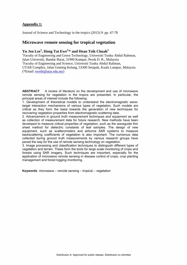
Appendix 1:

Journal of Science and Technology in the tropics (2013) 9: pp. 47-78

Microwave remote sensing for tropical vegetation

Yu Jen Lee1, Hong Tat Ewe

2,* and Hean Teik Chuah

2

1Faculty of Engineering and Green Technology, Universiti Tunku Abdul Rahman,

Jalan Universiti, Bandar Barat, 31900 Kampar, Perak D. R., Malaysia 2Faculty of Engineering and Science, Universiti Tunku Abdul Rahman,

UTAR Complex, Jalan Genting Kelang, 53300 Setapak, Kuala Lumpur, Malaysia

(*Email: [email protected])

ABSTRACT A review of literature on the development and use of microwave remote sensing for vegetation in the tropics are presented. In particular, the principal areas of interest include the following: 1. Development of theoretical models to understand the electromagnetic wave-target interaction mechanisms of various types of vegetation. Such models are critical as they form the basis towards the generation of new techniques for recovering vegetation properties from electromagnetic scattering data. 2. Advancement in ground truth measurement techniques and equipment as well as collection of measurement data for future research. New methods have been developed to measure critical properties of vegetation, such as the waveguide thin sheet method for dielectric constants of leaf samples. The design of new equipment, such as scatterometers and airborne SAR systems to measure backscattering coefficients of vegetation is also important. The numerous data collected during ground truth measurements by various research groups have paved the way for the use of remote sensing technology on vegetation. 3. Image processing and classification techniques to distinguish different types of vegetation and terrain. These form the tools for large scale monitoring of crops and forests using SAR imagery. Such techniques are important, especially for the application of microwave remote sensing in disease control of crops, crop planting management and forest logging monitoring. Keywords microwave – remote sensing – tropical – vegetation


mailto:[email protected]

INTRODUCTION

The use of microwave remote sensing has been advancing rapidly and has been

targeted as a primary solution to earth resource monitoring and management [1].

There is currently substantial existing work being done on the use of remote

sensing for various media, such as sea ice and ocean [2, 3]. In remote sensing of

tropical vegetation, observations of the electromagnetic fields scattered or emitted

by vegetation are used to characterize the physical properties and conditions of the

plants. Large-scale information obtained from such methods is important towards

applications such as the monitoring of agricultural crops and the maintenance of

tropical forests.

In the tropics, such as Asian countries, where rice is the staple food, the

capability to predict the yield of paddy for a particular year may assist government

agencies in the planning of food resources for its people. The use of remote sensing

as a tool to enable the use of crop models for yield prediction and other

applications has been recommended [4]. In terms of monitoring of large areas of

crops, the use of remote sensing images with the proper image classification

techniques may assist towards the control of diseases or natural hazards, thus

reducing the losses of both farmers and the government, where the export of the

crops may play a huge role towards the country’s economy. There has been

reported work on using electromagnetic data to discriminate fungal disease

infestation in oil palm [5].

With the current global focus shifting towards climate change and

environmental issues, the use of remote sensing towards the maintenance and

monitoring of tropical forests is also being considered. Logging activities and

deforestation are issues currently being tackled by several tropical countries, such

as in Brazil, where the Amazon rain forests are located and also in the rain forests

in Malaysia and Indonesia. Illegal logging has caused losses in millions of dollars

for these countries. Such activities also contribute towards the extinction of several

indigenous species of flora and fauna unique to these rain forests. Due to the vast

amount of areas covered by such virgin forests, it is impossible for park rangers to

cover the entire landscape to counter illegal logging or deforestation. Several

efforts had been made to propose the use of remote sensing to monitor the tropical

rain forests, such as the development of a monitoring system for tropical rainforest

management by a joint research group from Malaysia and Japan [6].

Regardless of how remote sensing is to be applied towards vegetation, it is

important to note that the development of proper theoretical models, the collection

of measurement data as well as the advancement of image classification techniques

are required in order to realize the potential of using remote sensing techniques for

such purposes. In this paper, the collection of such methods and their principal

results are reported, with focus given primarily on tropical vegetation such as

paddy, oil palm and forests.

THEORETICAL MODELING OF TROPICAL VEGETATION

In this section, several theoretical models developed to better understand the

relationship between the scattering properties of tropical vegetation and

microwaves are reported. In addition, models developed to model certain

parameters of tropical vegetation are also discussed. The models discussed below

are but a few of the current work being done to meet this task.

Paddy

Rice plays an integral role as the staple food of most Asians and is an important

agricultural crop. In China and Malaysia, the planting of paddy is important to

ensure the production of sufficient food source for the people. Due to its


importance, emphasis has been given to find methods to predict the yield of rice

and also to monitor the growth of paddy [4]. There has been a growing interest

towards the development of proper theoretical models to understand the scattering

properties of paddy.

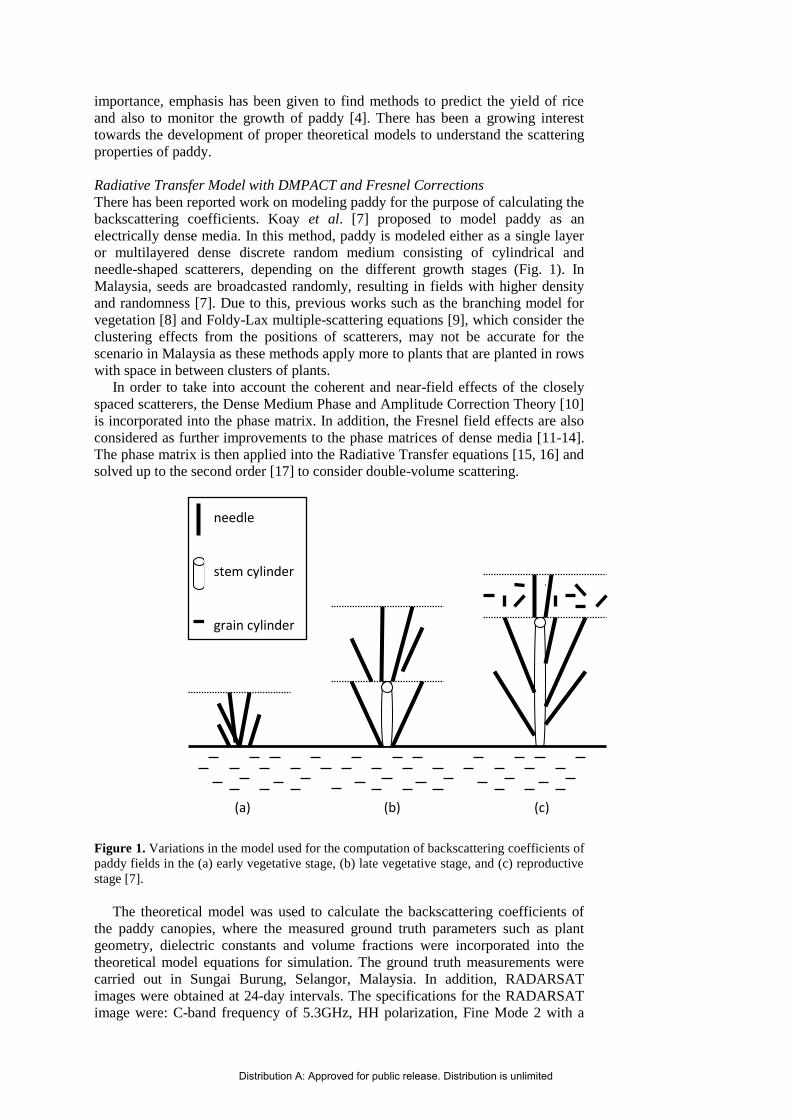
Radiative Transfer Model with DMPACT and Fresnel Corrections

There has been reported work on modeling paddy for the purpose of calculating the

backscattering coefficients. Koay et al. [7] proposed to model paddy as an

electrically dense media. In this method, paddy is modeled either as a single layer

or multilayered dense discrete random medium consisting of cylindrical and

needle-shaped scatterers, depending on the different growth stages (Fig. 1). In

Malaysia, seeds are broadcasted randomly, resulting in fields with higher density

and randomness [7]. Due to this, previous works such as the branching model for

vegetation [8] and Foldy-Lax multiple-scattering equations [9], which consider the

clustering effects from the positions of scatterers, may not be accurate for the

scenario in Malaysia as these methods apply more to plants that are planted in rows

with space in between clusters of plants.

In order to take into account the coherent and near-field effects of the closely

spaced scatterers, the Dense Medium Phase and Amplitude Correction Theory [10]

is incorporated into the phase matrix. In addition, the Fresnel field effects are also

considered as further improvements to the phase matrices of dense media [11-14].

The phase matrix is then applied into the Radiative Transfer equations [15, 16] and

solved up to the second order [17] to consider double-volume scattering.

Figure 1. Variations in the model used for the computation of backscattering coefficients of

paddy fields in the (a) early vegetative stage, (b) late vegetative stage, and (c) reproductive

stage [7].

The theoretical model was used to calculate the backscattering coefficients of

the paddy canopies, where the measured ground truth parameters such as plant

geometry, dielectric constants and volume fractions were incorporated into the

theoretical model equations for simulation. The ground truth measurements were

carried out in Sungai Burung, Selangor, Malaysia. In addition, RADARSAT

images were obtained at 24-day intervals. The specifications for the RADARSAT

image were: C-band frequency of 5.3GHz, HH polarization, Fine Mode 2 with a

(a) (b) (c)

needle

stem cylinder

grain cylinder


resolution of about 8 m and an incident angle range of 39°–42°. Table 1 shows the

model variation used for the different growth stages of rice crops, which

corresponds to the plant age and dates of the RADARSAT image acquired.

Table 1. Variations in the model for different growth stages [7].

Date Test Field Age (days) Model Variation

20-09-2004 1

4

5

6

27

26

29

21

Early vegetative

14-10-2004 1

4

5

6

51

50

53

45

Late vegetative

06-11-2004 1

4

5

6

75

74

77

69

Early reproduction

The model was used to calculate the HH-polarized backscattering coefficients

of several test fields at a frequency of 5.3GHz and at an incident angle of 41° in

order for comparisons with the RADARSAT data. Figure 2 shows the comparison

between the model prediction and the actual backscattering coefficients calculated

from the RADARSAT image for different stages of growth.

It was observed that the total backscattering coefficient increased during the

vegetative stages of the paddy plants as the plants grew taller and denser, but

decreased slightly at the reproductive stage, which might be due to halted growth

of plants and the dying off of smaller plants. The results show good matching in

general, but errors of about 2 dB were noticed at the age of 50 days. Such errors

were expected since the ground truth measurements were not exact statistical

representations of actual fields and might not be accurate. Another possible reason

could be the needle shape used to model the leaves, which might not be suitable as

some leaves could be wider in dimension.


Figure 2. Comparisons of theoretical and measured HH-polarized backscattering

coefficients at different stages of growth [7].

Comparisons between the dense medium model and the Monte Carlo

simulations were also carried out for VV-polarized backscattering coefficients

based on parameters given in [18]. Figure 3 shows that there was not much

difference in the results when the plants had a lower biomass when they were

young. However, as the plants grew and the biomass increased, the dense medium

model gave a better match with the ERS-1 data obtained at Samarang [18] and

Akita [19] due to the higher density of the canopy.

Figure 3. Comparisons of the backscattering coefficients obtained through the dense

medium model, Monte Carlo simulations, and ERS-1 data with respect to the plant biomass

[7].

In summary, a theoretical model developed for paddy fields using Radiative

Transfer theory was proposed [7] with consideration given to the coherent and

near-field effects of closely packed scatterers by incorporating the DM-PACT and


Fresnel correction terms in the phase matrix of the paddy canopy. Multiple volume

scattering was also considered by incorporating second-order solutions of the

Radiative Transfer theory. Utilizing ground truth measurements obtained for an

entire season at Sungai Burung, Selangor, Malayia, a theoretical analysis using the

model was carried out (detailed discussion of the analysis can be found in [7]). It

was found that multiple-volume scattering effects are important in the calculation

of cross-polarized backscattering coefficients and will be critical for applications

involving polarimetric data. Coherent effects need to be considered at lower

frequencies while Fresnel corrections are more important at higher frequencies.

The simulated results compared with RADARSAT images and the Monte Carlo

simulations showed promising results. A suggestion to improve the model is to use

elliptical disk-shaped scatterers in the phase matrix [20].

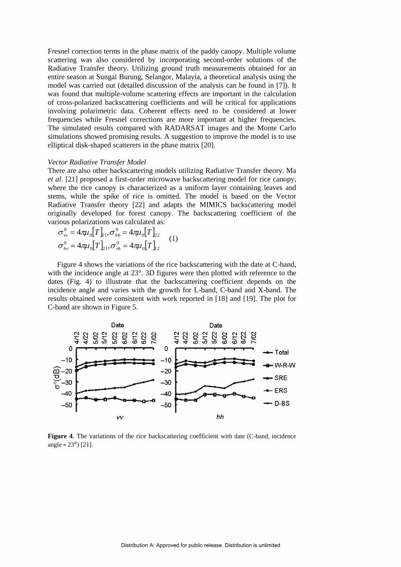
Vector Radiative Transfer Model

There are also other backscattering models utilizing Radiative Transfer theory. Ma

et al. [21] proposed a first-order microwave backscattering model for rice canopy,

where the rice canopy is characterized as a uniform layer containing leaves and

stems, while the spike of rice is omitted. The model is based on the Vector

Radiative Transfer theory [22] and adapts the MIMICS backscattering model

originally developed for forest canopy. The backscattering coefficient of the

various polarizations was calculated as:

120

0

210

0

220

0

110

0

4,4

4,4

TT

TT

vhhv

hhvv

(1)

Figure 4 shows the variations of the rice backscattering with the date at C-band,

with the incidence angle at 23°. 3D figures were then plotted with reference to the

dates (Fig. 4) to illustrate that the backscattering coefficient depends on the

incidence angle and varies with the growth for L-band, C-band and X-band. The

results obtained were consistent with work reported in [18] and [19]. The plot for

C-band are shown in Figure 5.

Figure 4. The variations of the rice backscattering coefficient with date (C-band, incidence

angle = 23°) [21].


Figure 5. C-band HH polarization [21].

Single Layer Radiative Transfer Model

Shao et al. [23] successfully predicted the radar backscatter behaviour of rice by

using an established Radiative Transfer model for vegetation canopies developed

by Sun et al. [24] on rice. The study focused on the temporal characteristics of rice

backscatter as a function of polarization at C-band. This study was carried out in

the Zhaoqing test site located in Guangdong Province in Southern China. The

multi-temporal RADARSAT image set comprised of 7 scenes acquired in Standard

Mode from April to July, 1997. Rice physical measurements were carried out

during the period of the RADARSAT acquisition. The fresh biomass of rice was

determined by:

M = [1000/a 1000/b] Wf N (2)

where a is the row spacing; b, the line spacing; Wf, the fresh weight of each rice

seedling; and N, the numbers of rice seedling of each cluster. The dielectric of rice

was calculated from the gravimetric water content using the empirical Dual-

dispersion model [25].

The model was used to generate backscatter coefficients for all polarizations. It

was found that for HH polarization, the generated data managed to fit the few

RADARSAT observations reasonably well (Fig. 6).

Further analysis of the generated backscatter coefficients shows that at a 45°

incidence angle, crown backscatter at HH and HV polarization increases as the rice

grows. However, at VV polarization the crown backscatter increases at the early

stage of the rice growth cycle and then stays relatively constant for the rest of the

rice growth cycle, which corresponds to results reported in [18]. Further research is

needed to fully utilize the model’s capabilities.


Figure 6. Comparing model results with RADARSAT observations in 1997 [23].

Coherent Electromagnetic Model

Other works on theoretical modeling of rice include work done by Fortuny-Guasch

et al. [26] and Ma et al. [27]. In [26], a physics-based coherent electromagnetic

model tailored for the computation of radar backscatter from rice was developed.

The model considers the rice as an arrangement of plants over a flooded soil, where

the plants are modeled as clusters of dielectric cylinders. The results show that the

co-polar backscattering coefficients obtained by the model are similar to the

measured ones, but the cross-polar scattering obtained is much lower. Future

consideration into multiple scattering between stems was suggested as an

improvement to the current model.

Radiative Transfer Model with Lindenmayer System

In [27], the employment of the Lindenmayer system (L-system) [28] and computer

graphics technique to describe the realistic structure of the rice crops was studied.

On the basis of such method, according to the physical interaction principle

between electromagnetic wave and vegetation, the intensity of scattered field of

each scatterer was calculated. By coherent addition of the individual scattered field

of each scatterer, the total backscattered field of the crop canopy can be obtained

and the backscattering coefficients can be calculated. The simulation results were

compared with the measurement data obtained via scatterometer. The results show

that the predication of backscatter is roughly identical to the measurement,

especially when the incidence angle is between 20° and 50°.

Studies have also been conducted on relating physical properties of the rice to

the microwave backscatter. Using the proper algorithms and models, the variations

in the backscatter are compared with variations in certain parameters in the rice.

Modeling of Rice Parameters

The modeling of dielectric microwave properties of rice using the Debye-Cole

dual-dispersion model of vegetation was studied in [29]. Results show that the

dielectric constant of rice varies at different growth stages. The dielectric constant

increases during the transplant to seedling developing period but decreases after

that. On the other hand, microwave frequency, gravimetric moisture content of rice,

temperature and density of dry rice canopy have an influence on dielectric constant.

In the study, salinity had no effect on the dielectric constant.

The mapping of rice biomass was done using ALOS/PALSAR imagery [30]. By

integrating a rice canopy scattering model [31], the spatial distribution of paddy


rice biomass was simulated. Plant height and density were the two most

determinant biophysical parameters related to rice biomass, which could be

retrieved with an error of less than 6 cm and 30/m2, respectively. Thus, the biomass

could be estimated with an adjusted residual of 200 g/m2. The results indicate that

the designed approach was useful to quantitatively estimate the carbon absorption

from the atmosphere during the growing season of rice and demonstrated the

potentials of using ALOS/PALSAR data for the mapping of rice biomass using the

microwave canopy scatter model.

Another important parameter relating to microwave backscatter is the leaf area

index (LAI). Stephen et al. [32] demonstrated this by modeling the flooded rice

field as a single layer of discrete scatterers over a reflecting surface using the

Distorted Born Approximation. At C-band, the VV polarization radar backscatter

decreased with increasing LAI over the observed range of LAI. Further

investigations using the simple model showed that the decrease was related to the

domination of direct-reflected backscatter over the direct component. Model

calculations suggested that at very low LAI the radar backscatter should increase

with LAI.

Inoue et al. [33] observed unique interactions between each of the microwave

backscatter coefficients at all combinations of five frequencies (Ka, Ku, X, C and

L), all polarizations (HH, VH, HV and VV) and four incident angles (25°, 35°, 45°

and 55°) and vegetation variables such as leaf index area (LAI), biomass and grain

yield. The study revealed that the realistic cropping condition of rice would allow

further quantitative insight on the interaction of backscatter with vegetation.

Oil Palm

Besides paddy, oil palm is another commodity that is important in the tropics. Palm

oil is viewed as a potential biofuel source in the future as the amount of fossil fuel

dwindles. It has also found uses as key ingredients in a variety of areas, such as

cooking oil, soaps and glycerol. Countries such as Indonesia, Malaysia, Nigeria

and Colombia are but a few of the tropical countries producing palm oil with the

growth of oil palm plantations.

3D Model with Radiative Transfer Theory

Izzawati et al. [34] adapted a 3D radar backscatter model originally designed for

forest canopies [35] to simulate high resolution images of polarimetric radar

backscatter of oil palm plantations at different growth stages. The main purpose

was to examine the relationships between the backscatter and texture and crop

status in order to invert the latter from space borne SAR data. The individual

crowns were modeled as hemispheres and distributed in a triangular pattern found

in oil palm plantations. Polarimetric radar backscatter was then simulated for C and

L band at high spatial resolution for a range of growth stages and LAI.

The original 3D radar backscatter matter was based on the Radiative Transfer

equation for a forest canopy comprising a crown layer, trunk layer and rough-

surface ground boundary. For the study, steps were taken to ensure the production

of reliable oil palm plantation stands at different growth stages to be used as input

in the model. Simulations were then carried out on the oil palm plantation using the

theoretical model at C and L band.

Multipolarized high resolution images (0.5 m) were simulated using the model

at years 2.5, 6.5 and 8.5 for C-band and at years 2.5, 4.5 and 6.5 for L-band (Fig. 7,

8). The estimation of the mean radar backscatter of C and L bands at HH, HV and

VV polarizations were also completed. A texture analysis was also done using

directional semivariograms. Early modeling results indicate the potential of using

mean backscatter and semivariance measures to discriminate oil palm stand age.


Figure 7. C-band simulation at age 2.5, 6.5 and 8.5 years [34].

Figure 8. L-band simulation at age 2.5, 4.5, and 6.5 years [34].

Tropical Forest There has been a multitude of reported work focusing on the modeling of

vegetation in general [8, 11-13, 17, 35, 36]. Some of these models actually form

the basis for the model developed for paddy and oil palm. Many of these models

were previously validated on temperate climate forests, such as Boreal or Cypress

forests. In this section, modeling done and validated on tropical forests is discussed.

Hybrid Coherent Scattering Model

Thirion et al. [37] looked into several earlier models and concluded that there is a

need to study the different scattering mechanisms involved in the forest by means

of a fully coherent scattering model (COSMO). They proposed a new hybrid model

derived from the RVoG model. Retrieval studies indicated that the model seems to

be more adapted to the P-band. COSMO is a coherent descriptive model that is

applied to radiometry, interferometry and polarimetry. In the paper, the model was

used to simulate SAR data for Mangrove (tropical) and Nezer (temperate) forests

for P-band and L-band. The comparisons between the simulations and the real SAR

data were satisfactory in radiometry for both types of vegetation. The model also

showed good ability to simulate the interferometric data and polarimetric behaviour

of the vegetation mentioned.

Multilayer Radiative Transfer Model

The use of multilayer models to model vegetation has also been proposed [11, 17].

Ewe et al. [11] treated vegetation as an electrically dense media. Utilizing the

Radiative Transfer theory, the array phase correction factor was incorporated into

the phase matrices of the nonspherical scatterers to take into account the coherent

effect between scatterers. In addition, the amplitude and Fresnel phase corrections

were also included when the Fresnel factor was larger than /8. The improved

phase matrix was then included into the Radiative transfer formulation. Finally this

formulation was solved iteratively up to the second order to incorporate the

multilayer effects. It was found that the measurement results for Japanese cypress

and boreal forest with multifrequency and multipolarization data showed good

agreement with the theoretical predictions from the model. There is huge potential

for the model to be used to model for tropical dense forest.

Karam et al. [17] came up with a two layer scattering model for trees and tested

it on both coniferous and deciduous trees. In the model, the two layers are the


crown layer and trunk layer above an irregular surface. Deciduous leaves, which

are quite common in tropical trees, are modeled as randomly oriented circular discs.

The advantages for this model is that it accounts for the first and second order

scattering within the canopy, fully accounts for the surface roughness in the

canopy-soil interaction terms, allows many branch sizes and orientation

distributions, and finally is valid over a wide frequency range for both deciduous

and coniferous vegetation.

Validation was carried out by applying the model to walnut and cypress trees. A

comparison between the backscattering measurements and the model predictions

was done. Additionally, the effects of frequency, second order interaction and

surface roughness effects were studied. It was found that in order to obtain good

matching between calculated and simulated backscattering coefficients, the branch

size distribution is important. The model discretized branch size distribution into

four sizes. Next, small branches and leaves generally contribute to the

backscattering coefficients at X-band. For deciduous trees, cross polarization at X-

band is dominated by stems rather than leaves. Lastly, soil moisture and soil

roughness are more important for HH polarization as they influence the trunk-soil

interaction contribution to the backscattering coefficients.

GROUND TRUTH MEASUREMENT OF TROPICAL VEGETATION

The development of theoretical models is important to understand the physics and

interaction between electromagnetic waves and vegetation. The results from these

studies also aid in the development and design of proper ground truth measurement

systems.

Development of Measurement Tools

One important aspect in the study of remote sensing is the design of measurement

tools to perform ground truth measurements.

Ground based scatterometers

Ground based scatterometer systems are popular methods for the collection of

backscattering data from agriculture vegetation such as paddy and oil palm. Due to

its importance, the development of ground based radar is as important as airborne

SAR. Koo et al. [38] reported the development of a ground based radar for

scattering measurements operating at C-band. Constructed from a combination of

commercially available components and in-house fabricated circuitry, the system

has full polarimetric capability for determining the complete backscattering matrix

of a natural target. A microwave sensor was constructed and installed onto a boom

truck (Fig. 9). Designed for short-range operations, a frequency-modulated (FM-

CW) configuration was employed for the scatterometer system. Table 2

summarizes the system’s specifications.


Figure 9. A photograph of the scatterometer system.

Figure 10 illustrates the simplified system block diagram, where the main

sections are the RF section, the antenna, the IF section and the data acquisition unit.

The system was tested in a low reflection outdoor environment [38]. The results

from the measurements in the tests were compared with the theoretical values to

evaluate the measurement accuracy.

Figure 10. The system block diagram [38].


1

Figure 11 shows one of the RCS measurement carried out. In general, it

was observed that the measured scattering matrices had good agreement

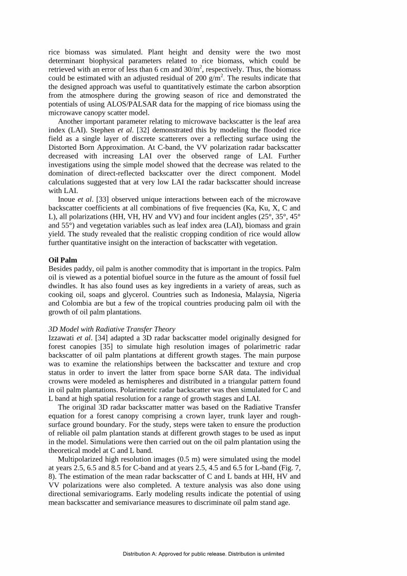
with the theory and the measurement accuracy was within ±1.5 dB in

magnitude and ±10° in phase. The scatterometer system has been used to

conduct in-situ backscattering measurements of tropical crops.

Table 2. Specifications of ground based scatterometer [38].

System Parameter Specification

System Configuration

Type FM-CW

Operating frequency, fc 6 GHz (C-band)

Operating wavelength, λ 5 cm

Sweep Bandwidth, B 400 MHz

Modulating frequency, fm 60 Hz

Polarization HH, VV, HV, VH

Polarization isolation 35 dB

Antenna gain, G 35 dB

Antenna 3 dB beamwidth, β 3°

Best possible range resolution, vR 0.375 m

Platform Boom truck

Platform height, h 25 m (vertical)

Measurement Capability Transmitter power, Pt 10 dBm

Received power, Pr –15 dBm to –92 dBm

°Dynamic range +20 dB to –40 dB

Measurement range, R 20 m to 100 m

Incident angle coverage, 0° – 70°

Minimum signal-to-noise ratio, SNR 10 dB

Effective range resolution, ΔR (~1.8 m at = 45°;4.5 m at

= 60°)


2

Figure 11. The measured power spectra of an 8” trihedral corner reflector [38].

There has also been a multitude of other developed ground based

scatterometers utilized for the remote sensing of tropical vegetation, in

particular rice crops. In [39, 40], an FM-CW scatterometer with four

parabolic antenna (L, S, C, X) configurations was designed and utilized

to collect microwave backscatter signatures of paddy over the entire rice-

growing season. An X-band scatterometer system named POSTECH

Polarimetric Scatterometer (POPOS) was designed and implemented by

Kim et al. [41] to obtain radar backscattering measurements of rice crops

over the whole period of rice growth at three polarization combinations.

The experience and success in the design and implementation of

various types of ground based scatterometers gives rise to the confidence

to develop airborne SAR systems.

Airborne SAR

There has been reported work on the development of airborne synthetic

aperture radars. Koo et al. [42] developed the Malaysian Airborne

Synthetic Aperture Radar (MASAR) for the purpose of earth resource

monitoring, such as paddy fields, oil palm and soil surface. This SAR

system is a C-band, single polarization, linear FM radar. The preparatory

studies on the conceptual design of the microwave system were presented

by Chan et al. [43]. The SAR system is capable of operating at moderate

altitudes with low transmit power and small swath width.


3

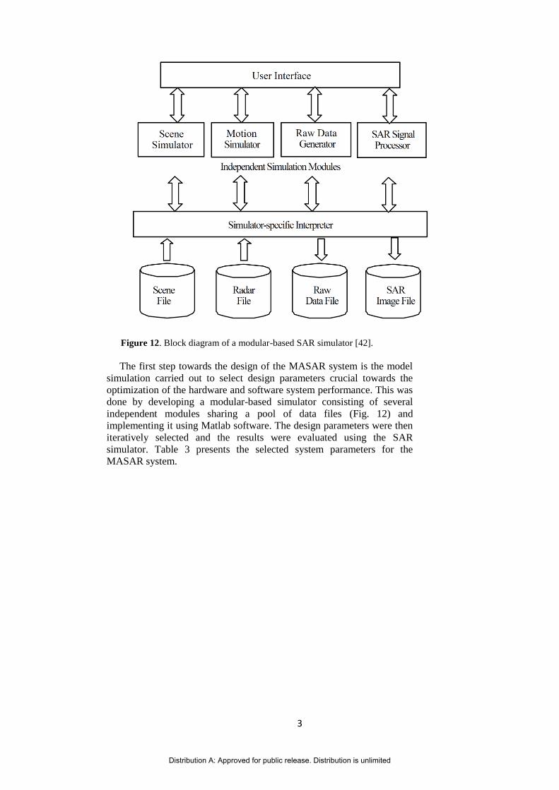
Figure 12. Block diagram of a modular-based SAR simulator [42].

The first step towards the design of the MASAR system is the model

simulation carried out to select design parameters crucial towards the

optimization of the hardware and software system performance. This was

done by developing a modular-based simulator consisting of several

independent modules sharing a pool of data files (Fig. 12) and

implementing it using Matlab software. The design parameters were then

iteratively selected and the results were evaluated using the SAR

simulator. Table 3 presents the selected system parameters for the

MASAR system.


4

Table 3. The MASAR specifications [42].

System Parameter Specification

Mode of operation Stripmap

Operating frequency, fc 5.3 GHz (C-band)

Bandwidth, B 20 MHz

Chirp pulse duration, p 20s

Pulse repetition frequency 1000 HZ

Transmitter peak power, Pt 100 W

Polarization Linear, VV

Antenna gain, G >18 dBi

Elevation beamwidth, βel 24°

Azimuth beamwidth, βaz 3°

Synthetic aperture length ~200 m

ADC sampling frequency 100 MHz

ADC quantization 12-bit

Data rate, d 100 Mbps

Recorder capacity 2 160 GB, SATA

Data take duration, Td >5 hours

°dynamic range 0 dB to –30 dB

Signal-to-noise ratio, SNR >10 dB

Best slant range resolution 7.5 m

Best azimuth resolution, ρa 7.5 m (2-looks)

Incident angle, 50°

Swath width, W ~8 km

Platform height, h 7500 m

Nominal platform speed, v0 100 m/s

Operating platform Pressurized aircraft

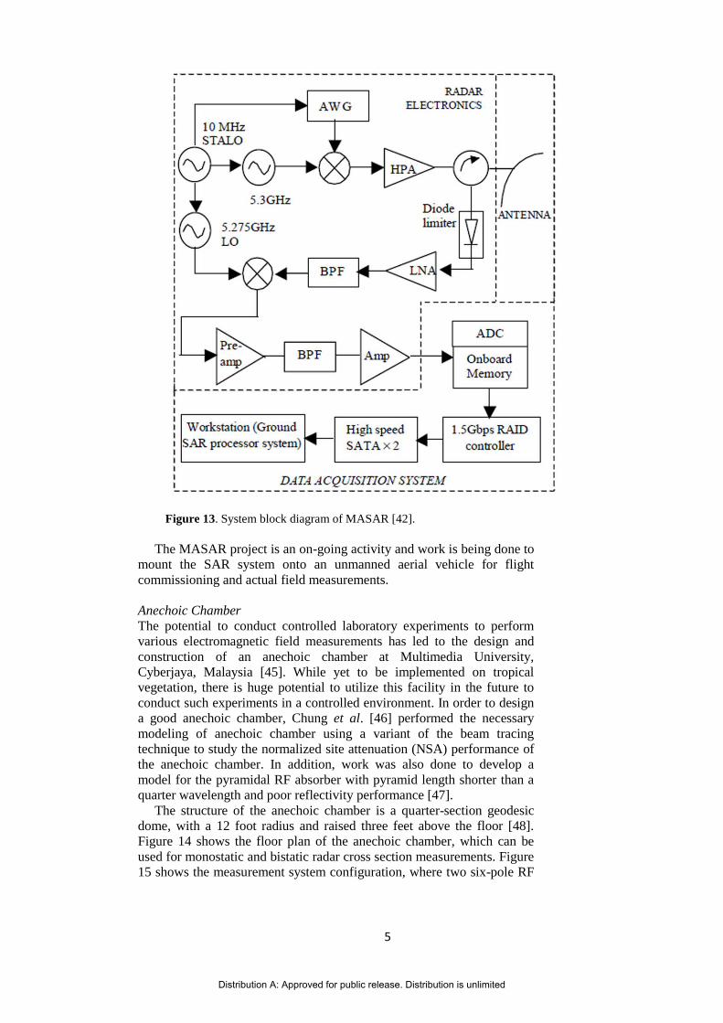
The functional block diagram for the MASAR system (Fig. 13)

consists of a microstrip antenna, a radar electronics subsystem and a data

acquisition system [for details, see [42]). A prototype RF transceiver for

both ranged detection and radar cross section (RCS) measurement was

also developed and verified in field experiments [44]. Finally, the

algorithm for the MASAR image formation was developed based on the

parallel implementation of the wavefront reconstruction theory, known as

the range-stacking algorithm. The range-stacking algorithm does not

require interpolation and does not suffer from truncation errors.


5

Figure 13. System block diagram of MASAR [42].

The MASAR project is an on-going activity and work is being done to

mount the SAR system onto an unmanned aerial vehicle for flight

commissioning and actual field measurements.

Anechoic Chamber

The potential to conduct controlled laboratory experiments to perform

various electromagnetic field measurements has led to the design and

construction of an anechoic chamber at Multimedia University,

Cyberjaya, Malaysia [45]. While yet to be implemented on tropical

vegetation, there is huge potential to utilize this facility in the future to

conduct such experiments in a controlled environment. In order to design

a good anechoic chamber, Chung et al. [46] performed the necessary

modeling of anechoic chamber using a variant of the beam tracing

technique to study the normalized site attenuation (NSA) performance of

the anechoic chamber. In addition, work was also done to develop a

model for the pyramidal RF absorber with pyramid length shorter than a

quarter wavelength and poor reflectivity performance [47].

The structure of the anechoic chamber is a quarter-section geodesic

dome, with a 12 foot radius and raised three feet above the floor [48].

Figure 14 shows the floor plan of the anechoic chamber, which can be

used for monostatic and bistatic radar cross section measurements. Figure

15 shows the measurement system configuration, where two six-pole RF


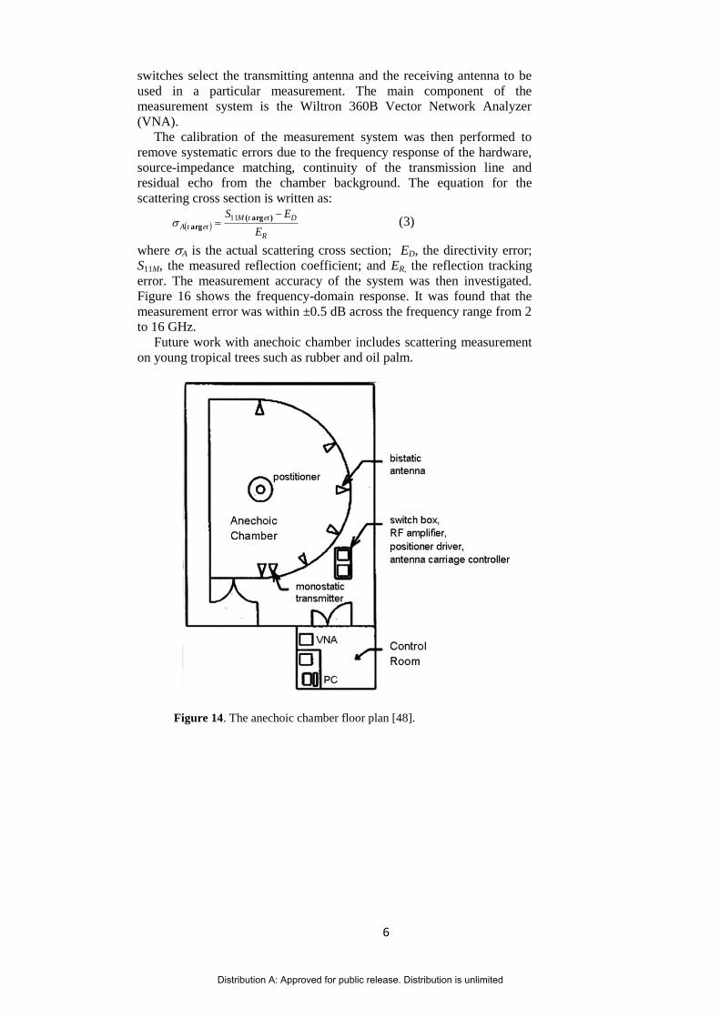
6

switches select the transmitting antenna and the receiving antenna to be

used in a particular measurement. The main component of the

measurement system is the Wiltron 360B Vector Network Analyzer

(VNA).

The calibration of the measurement system was then performed to

remove systematic errors due to the frequency response of the hardware,

source-impedance matching, continuity of the transmission line and

residual echo from the chamber background. The equation for the

scattering cross section is written as:

R

DettMettA

E

ES

)arg(arg

11 (3)

where A is the actual scattering cross section; ED, the directivity error;

S11M, the measured reflection coefficient; and ER, the reflection tracking

error. The measurement accuracy of the system was then investigated.

Figure 16 shows the frequency-domain response. It was found that the

measurement error was within ±0.5 dB across the frequency range from 2

to 16 GHz.

Future work with anechoic chamber includes scattering measurement

on young tropical trees such as rubber and oil palm.

Figure 14. The anechoic chamber floor plan [48].


7

Figure 15. The measurement-system configuration [48].

Figure 16. A comparison between the measured and theoretical frequency

behaviour of the monostatic RCS of a 3” sphere after time-domain gating [48].

Moisture sensors

Moisture sensors are important measurement tools as they can provide

parameter inputs to the developed theoretical models. The data collected

from these sensors are also useful to verify the results obtained from

theoretical models as well. The dielectric properties of a non-magnetic

material play an important role in the interaction with electromagnetic

waves. Understanding this importance, Khalid et al. [49] proposed the


8

development of planar microwave moisture sensors. In the study, the

close relationship between moisture content and dielectric properties for

both hevea rubber latex and oil palm fruits were investigated.

The attenuation of the microstrip sensor against the moisture content

for hevea latex and for various thickness of protective layer is shown in

Figure 17. The deviation of the test result of the moisture parameter is

less than 1% compared to that obtained by Standard Gravimetric method.

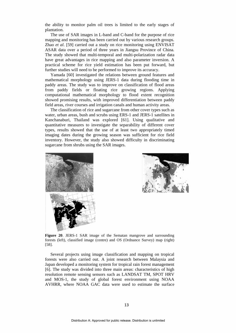
The microstrip sensor was integrated into the designed ripeness indicator

prototype for oil palm fruits (Fig. 18). The detected current from the

meter is related to the moisture content of mashed mesocarp and finally

the stage of the ripeness can be determined.

A dual frequency sensor was also developed to measure moisture

content of the rubber latex. The design is based on the measurement of

magnitudes of the near field reflection at two frequencies in the X-band,

8.48 and 10.69 GHz. The design also replaces the conventional open horn

antenna with microstrip radiating patches. This construction makes the

sensor more versatile and compact and removes the temperature effect on

moisture content measurements without involving phase measurement. A

calibration equation was then found that instantly gives moisture content

of the samples using the developed sensors. The system was tested using

rubber latex and had predicted moisture content with a standard error of

less than ± 0.4% compared to standard oven drying techniques and a

mean error of less than ±1.3% in the temperature range of 25°C to 60°C. The prototype version of the dual-frequency moisture meter is shown in

Figure 19. Future consideration for this work is to expand the method to

construct moisture sensors for other products such as palm oil.


9

Figure 17. Variation of attenuation or insertion loss with moisture content for

microstrip sensors [49].

Figure 18. A prototype of ripeness meter for oil palm fruit [49].


10

Figure 19. A prototype model for dual-frequency microwave liquid moisture

meter [49].

The development of various ground truth measurement systems and

sensors has allowed researchers to conduct year long measurements at

various sites.

Measurement Data Collection

The collection of various parameters from tropical vegetation is essential

towards the validation of theoretical models and image classification

techniques for microwave remote sensing and also for future references.

Most parameters can be obtained directly through simple measurements,

such as plant height, trunk diameter and circumference, leaf length, etc.

Other parameters however may require the use of equations from various

theoretical models to calculate. As such, the development of such models

is important as they indirectly contribute towards the application of

remote sensing for earth terrain monitoring. In addition, there are also

plenty of measurement data collected via different techniques on tropical

vegetation. Some of these measurements were carried out for the entire

growth cycle of the plants and may provide crucial data for the remote

sensing of such media.

Dielectric constant is an important biophysical parameter that plays a

crucial role in the validation of theoretical models and the development of

yield prediction models for tropical crops. Chuah et al. [50] explored the

accuracy of two theoretical models that were used to estimate the

dielectric constants of leaves from two tropical crops (rubber and oil palm)

as a function of moisture content at X-band. The models being studied

were the simple dielectric theory by Fung and Fung [51] and the dual-

dispersion model by Ulaby and El-Rayes [52]. Utilizing the waveguide

thin sheet technique to measure the dielectric constant of the leaves, they

were able to successfully evaluate the performance of both models. It was

found that the dual-dispersion model gave a more accurate estimation of

the dielectric constants and thus confirmed its applicability to the leaves

of rubber and oil palm in future research work.

Other parameters important towards yield prediction models and

growth assessment are above ground biomass (AGB) and stem volume.

Previous works measured oil palm biomass and stem volume from

mature oil palm by destructive sampling which involved weighing all the

major components of biomass and stem volume for different ages [53].


11

These studies extrapolated the data from the destructive measurements on

a few palms from each age group, but the procedure might be

underestimated due to restricted sampling areas. In addition, the method

is tedious and time consuming.

Asari et al. [54] proposed the measurement of the parameters using the

non-destructive sampling as a preliminary study towards the development

of a prediction model for the estimation of oil palm above ground

biomass and stem volume using remote sensing data. The main aim of the

study was to estimate the two parameters at different ages using the non-

destructive method and to study the relationship between oil palm

biomass and several parameters such as crown width, height, the diameter

of breast height, length and depth of petiole of oil palm stand. The study

found that the trunk biomass contributed a major portion of the oil palm

biomass, about 86 to 95% from the total AGB. The study also discovered

that the age of the oil palm was directly correlated to above ground

biomass, while stem volume was inversely correlated with the age of oil

palm. A full scale study combining the ground information and remote

sensing is being conducted.

Vegetation water content (VWC) plays a significant role in the

retrieval of soil moisture from microwave remote sensing and also in

forest and agricultural studies such as drought assessment and yield

prediction. Kim et al. [55] reported that previous studies analyzed the

relationship between NDVI and VWC and developed techniques to

estimate VWC and other biophysical variables. They went a step further

and examined the relationship between polarimetric radar data, VWC,

LAI and normalized difference vegetation index (NDVI) using soybean

and rice, focusing on the use of radar vegetation index (RVI) to estimate

VWC. In order to perform the study, the backscattering coefficients for

L-, C- and X-bands, vegetation indices (RVI, NDVI and LAI) and VWC

were observed over rice and soybean growth cycles. Retrieval equations

were then developed for estimating VWC using the RVI of both crops.

The study concluded that L-band RVI was well correlated with VWC,

LAI and NDVI compared to C- and X-band and thus achieved the most

accurate VWC retrievals. It should be noted however, that the

investigation only focused on a 40° single incidence angle observing

system since this study would be employed on the NASA Soil Moisture

Active Passive satellite (SMAP) in the future. As such further studies

may explore the effects of the incidence and azimuth angles.

The measurement of radar backscatter data from paddy, especially

over the entire growth cycle is also important towards the development of

yield prediction models via remote sensing. There is a substantial amount

of reported work on the radar measurements microwave backscattering

coefficients of rice plants [39-41, 56]. In these papers, the measurements

of the rice plants were carried out using constructed ground based

scatterometers over multifrequency and multipolarization covering an

entire rice growing season. The locations of the measurements covered

areas in Japan, China and Korea. In addition, measurement of other

parameters such as LAI, biomass, etc. were also performed on the paddy.

While the earlier works performed radar measurements using ground

based scatterometers, the attempts to use space borne satellites for such

measurements are few. Kurosu et al. [19] presented their measurements

on monitoring rice crop growth from space using the European Remote

Sensing satellite 1 (ERS-1). The SAR measurements were performed at


12

the rice fields of Akita Prefectural College of Agriculture covering two

growing seasons in 1992 and 1993 and were the first attempt to monitor

rice crop growth from space covering all growth stages.

Tropical forest biomass estimation is important for global research.

Such correlation analysis forms the base for developing models and

techniques to estimate tropical forest biomass from remote sensing data.

Yang et al. [57] utilized LANDSAT TM data and the biomass data

collected from main tropical forest vegetation types in Xishuangbanna,

China for studying the correlations between the biomass of vegetation

types. The study found that the relationships between the biomass of

monsoon tropical forest and LANDSAT TM6 and TM7 were the

strongest. TM6 was positively and significantly (at 95% level of

confidence) related to forest biomass while TM7 was inversely and

significantly (at 95% level of confidence) related to forest biomass. Lastly, the LANDSAT TM was observed to be not significantly (at 95%

level of confidence) related to the forest biomass for both the

mountainous tropical forest and the seasonal ever-green broadleaf forest.

IMAGE PROCESSING TECHNIQUES FOR THE REMOTE

SENSING OF TROPICAL VEGETATION

Remote sensing has proved to be an extremely convenient method to

monitor large areas of agriculture crops or forests. The use of SAR

images from airborne or space borne radar allows the coverage of large

areas and provides huge amount of information. Image processing thus

plays a crucial role, as it is important for researchers to be able to

differentiate between areas of interest from other landscape captured

within the image. The proper image processing tool will be required in

order to correctly analyze the image and highlight the areas of interest.

Chuah et al. [1] reported the use of fractal dimension of images as an

additional input to a neural network classifier to classify different areas of

interest. Preliminary results showed that fractal analysis was useful

towards the classification of sea, urban, forested and paddy areas. Ouchi

et al. [58] explored the comparison between the use of optical and radar

images on the classification of mangrove, virgin forests and oil palm

plantation with the ground truth data collected from the field survey.

Visible and infrared images were acquired using MOS-1b, while SAR

images from JERS-1 at L-band and ERS-2 at C-band were also obtained.

The optical images were capable of classifying deforestation areas, but

applications to mangrove forests were limited. SAR images performed

better and were capable of differentiating the mangrove from virgin

forests [58]. It was concluded that due to the longer penetration depth of

L-band, the JERS-1 performed better than the ERS-2, even though both

the mangrove and virgin forests had similar biomass well above the

saturation range of the L-band RCS. The top image in Figure 20 shows

the 3-look image of the Sematan test site in 1993, with the difference in

intensity between the mangrove and neighbouring virgin forests about

6dB, making it possible to extract the mangrove area. The classified

image is shown in the middle of Figure 24 and shows good agreement

with the OS (Ordnance Survey) map at the bottom. The reason in the

difference in intensity is associated with whether the ground is covered

by water or undergrowth, which is supported by the difference in image

intensity between dry and wet seasons. Lastly, the study also showed that


13

the ability to monitor palm oil trees is limited to the early stages of

plantation.

The use of SAR images in L-band and C-band for the purpose of rice

mapping and monitoring has been carried out by various research groups.

Zhao et al. [59] carried out a study on rice monitoring using ENVISAT

ASAR data over a period of three years in Jiangsu Province of China.

The study showed that multi-temporal and multi-polarization radar data

have great advantages in rice mapping and also parameter inversion. A

practical scheme for rice yield estimation has been put forward, but

further studies will need to be performed to improve its accuracy.

Yamada [60] investigated the relations between ground features and

mathematical morphology using JERS-1 data during flooding time in

paddy areas. The study was to improve on classification of flood areas

from paddy fields or floating rice growing regions. Applying

computational mathematical morphology to flood extent recognition

showed promising results, with improved differentiation between paddy

field areas, river courses and irrigation canals and human activity areas.

The classification of rice and sugarcane from other cover types such as

water, urban areas, bush and scrubs using ERS-1 and JERS-1 satellites in

Kanchanaburi, Thailand was explored [61]. Using qualitative and

quantitative measures to investigate the separability of different cover

types, results showed that the use of at least two appropriately timed

imaging dates during the growing season was sufficient for rice field

inventory. However, the study also showed difficulty in discriminating

sugarcane from shrubs using the SAR images.

Figure 20. JERS-1 SAR image of the Sematan mangrove and surrounding

forests (left), classified image (centre) and OS (Ordnance Survey) map (right)

[58].

Several projects using image classification and mapping on tropical

forests were also carried out. A joint research between Malaysia and

Japan developed a monitoring system for tropical rain forest management

[6]. The study was divided into three main areas: characteristics of high

resolution remote sensing sensors such as LANDSAT TM, SPOT HRV

and MOS-1, the study of global forest environment using NOAA

AVHRR, where NOAA GAC data were used to estimate the surface


14

temperature and evapotranspiration of Peninsula Malaysia, and zoning

technology using a combination of a GIS system with remote sensing

data processing system for managing tropical forest environment.

Another similar project, where remote sensing was used to extract

environmental information of a tropical mountainous forest was carried

out in a National Park in Vietnam [62]. Parameters crucial towards the

management of the mountainous forest, such as wetness, groundwater

conditions, geological structure and land cover changes were successfully

extracted by application of remote sensing and GIS analysis. The Central

Africa Mosaic project (CAMP) also studied the use of ERS-1 images for

the purpose of tropical vegetation monitoring, combining the use of

thematic interpretation, data processing and new initiatives for large scale

radar maps [63].

The use of image processing techniques together with SAR images to

estimate different forest parameters were also researched. Foody et al.

[64] proposed the use of neural networks to estimate the diversity and

composition of a Bornean tropical rain forest using Landsat TM data. In

the study, a feedforward neural network was applied to estimate species

richness while a Kohonen neural network was used to provide

information on species composition. Another study focused on soil

moisture estimation using a remote sensing algorithm from LANDSAT

TM, ETM and ENVISAT images [65]. Preliminary results show that the

empirical model used to estimate soil moisure had a poor agreement with

the measured values. As such, further exploration into the model is

necessary.

Tropical forest carbon stock and biomass are important parameters in

forest management. Yang et al. [66] explored the possibility to estimate

carbon stock of tropical forest vegetation using LANDSAT TM data and

GIS data. A model to estimate biomass was formulated with the data of

forest fixed samples, GIS and LANDSAT TM images. Finally the carbon

stock was created from the biomass calculated using the above model.

The model has been found to be effective. Williams et al. [67] proposed

recovering tropical forest biomass from GeoSAR observations. The

airborne GeoSAR collects X-band and P-band InSAR data

simultaneously. It was shown that GeoSAR X-P interferometric data

alone may be used to recover tropical forest biomass, removing any

ambiguity associated with variation in ground conditions.

CONCLUSION

Remote sensing has been applied to tropical vegetation, both in

agriculture and forestry. The problem of remote sensing of vegetation can

be divided into three main categories: development of theoretical models,

ground truth measurement techniques, and equipment and image

processing.

There has been a multitude of scattering models developed to

understand the interaction between tropical vegetation and

electromagnetic waves. The use of Radiative Transfer theory is highly

popular, though there are other theories being utilized as well. Several

variations to the RT model are the multilayer model, DMPACT and

Fresnel corrections, combination with the Lindenmayer System and also

the Vector Radiative Transfer model. These extensions sought to improve


15

on the accuracy of backscatter predictions and serve as the basis for the

future development of inversion models.

The design and study of equipment to carry out measurements are

needed to obtain ground truth data from vegetation for the purpose of

model validation. There are research groups focusing on the development

of ground based and airborne scatterometers and SAR. An anechoic

chamber was also designed by a research team in MMU, Cyberjaya,

Malaysia, while moisture sensors have also been looked into. Lastly,

there is also research on image processing to improve on image

classification from spaceborne and airborne images to distinguish

between different vegetation types and other land areas.

There is still much work to be done on all areas in order to develop

more accurate techniques for the remote sensing of tropical vegetation. Acknowledgement – The authors would like to thank Advanced Agriecological

Research Sdn Bhd (AAR), Universiti Tunku Abdul Rahman (UTAR) and the

Ministry of Science, Technology and Innovation of Malaysia (MOSTI) for their

support in the project.

REFERENCES

1. Chuah H.T. (1997) An Overview of Microwave Remote Sensing

Research at the University of Malaya, Malaysia. Proceedings of IEEE

International Geoscience and Remote Sensing Symposium 3: 1421–

1423.

2. Golden, K.M.; Borup, D.; Cheney, M.; Cherkaeva, E.; Dawson, M.S.;

Kung-Hau Ding; Fung, A.K.; Isaacson, D.; Johnson, S.A.; Jordan, A.K.;

Jin An Kon; Kwok, R.; Nghiem, S.V.; Onstott, R.G.; Sylvester, J.;

Winebrenner, D.P.; Zabel, I.H.H. (1998) Inverse Electromagnetic

Scattering Models for Sea Ice. IEEE Transactions on Geoscience and

Remote Sensing 36(5): 1675–1704.

3. Fernandez D.E.; Chang P.S., Carswell J.R., Contreras R.F. and Frasier

S.J. (2005) IWRAP: The Imaging Wind and Rain Airborne Profiler for

Remote Sensing of the Ocean and the Atmospheric Boundary Layer

Within Tropical Cyclones. IEEE Transactions on Geoscience and


4. Guerif M., Launay M. and Duke C. (2000) Remote sensing as a tool

enabling the spatial use of crop models for crop diagnosis and yield

prediction. Proceedings of IEEE International Geoscience and Remote

Sensing Symposium 4: 1477–1479.

5. Lelong C.C.D., Roger J.-M., Bregand S., Dubertret F., Lanore M.,

Sitorus N.A., Raharjo D.A. and Caliman J.-P. (2009) Discrimination of

Fungal Disease Infestation in Oil-Palm Canopy and Hyperspectral

Reflectance Data. Proceedings of First Workshop on Hyperspectral

Image and Signal Processing: Evolution in Remote Sensing: 1–4.

6. Sawada H., Nakakita O., Awaya Y., Hamzah K.A. and Hassan A. (1991)

Development of Monitoring System for Tropical Rain Forest

Management in the Peninsula Malaysia: The Joint Malaysia-Japan

Research Project on Remote Sensing. Proceedings of IEEE

International Geoscience and Remote Sensing Symposium: Remote

Sensing: Global Monitoring for Earth Management 3: 1153–1156.

7. Koay J.Y., Tan C.P., Lim K.S., Saiful Bahari A.B., Ewe H.T., Chuah

H.T. and Kong J.A. (2007) Paddy Fields as Electrically Dense Media:

Theoretical Modeling and Measurement Comparisons. IEEE

Transactions on Geoscience and Remote Sensing 45(9): 2837–2849.


16

8. Yueh S. H., Kong J. A., Jao J. K., Shin R. T. and Le Toan T. (1992)

Branching Model for Vegetation,” IEEE Transactions on Geoscience

and Remote Sensing 30(2): 390–402.

9. Tsang L., Ding K. H., Zhang G., Hsu C. C. and Kong J. A. (1995)

Backscattering Enhancement and Clustering Effects of Randomly

Distributed Dielectric Cylinders Overlying a Dielectric Half Space

based on Monte-Carlo Simulations. IEEE Transactions on. Antennas

and Propagation 43(5): 488–499.

10. Chuah H.T, Tjuatja S., Fung A.K. and Bredow, J.W. (1996) A Phase

Matrix for a Dense Discrete Random Medium: Evaluation of Volume

Scattering Coefficient. IEEE Transactions on Geoscience and Remote

Sensing 34(5): 1137-1143.

11. Ewe H.T. and Chuah H.T. (2000). Electromagnetic Scattering from an

Electrically Dense Vegetation Medium. IEEE Transactions on

Geoscience and Remote Sensing 38(5): 2093-2105.

12. Fung A. K. and Chen M. F. (1987) Fresnel Field Interaction Applied to

Scattering from a Vegetation Layer. Remote Sensing of Environment.

23(1): 35–50.

13. Ewe H. T. and Chuah H. T. (2000) A Study of Fresnel Scattered Field

for Nonspherical Discrete Scatterers. Progress in Electromagnetics

Research 25: 189–222.

14. Fung A.K. (1994) Microwave Scattering and Emission Models and

Their Applications. Artech House, Norwood, Massachusetts.

15. Chandrasekhar S. (1960) Radiative Transfer. Dover, New York.

16. Ulaby F. T., Moore R. K. and Fung A. K. (1982) Microwave Remote

Sensing: Active and Passive, Vol. II. Artech House, Norwood,

Massachusetts.

17. Karam M. A., Fung A. K., Lang R. H. and Chauhan N. S. (1992) A

Microwave Scattering Model for Layered Vegetation. IEEE


18. Le Toan T., Ribbes F., Wang L. F., Floury N., Ding K. H., Kong J. A.,

Fujita M. and Kurosu T. (1997) Rice Crop Mapping and Monitoring

Using ERS-1 Data Based on Experiment and Modeling results. IEEE


19. Kurosu T., Suitz T., and Moriya T. (1995) Monitoring of Rice Crop

Growth from Space using ERS-1 C-Band SAR,” IEEE Transactions on

Geoscience and Remote Sensing 33(4): 1092–1096.

20. Koay J.Y., Ewe H.T. and Chuah H.T. (2008) A Study of Fresnel

Scattered Fields for Ellipsoidal and Elliptic-Disk-Shaped Scatterers.

IEEE Transactions on Geoscience and Remote Sensing 46(4): 1091–

1103.

21. Ma H.B., Zeng Q.M., Ma A.N. and Zhang T. (2000) Simulation and

Analysis for the Microwave Backscattering Coefficient of Rice.

Proceedings of IEEE International Geoscience and Remote Sensing

Symposium 2: 369–371.

22. Ulaby F.T., Sarabandi K., MacDonald K., Whitt M., and Dobson M. C.

(1990) Michigan Microwave Canopy Scattering Model. International

Journal of Remote Sensing 11, 1223–1253.

23. Shao Y., Liao J.J, Fan X.T. and Wang Y.H. (2002) Analysis of

Temporal Backscatter of Rice: A Comparison of RADARSAT

Observations with Modeling Results. Proceedings of IEEE


Sensing 1: 478–480.

24. Sun G., Simonett D., and Strahler A. (1991) A Radar Backscatter Model

for Discontinuous Coniferous Forests. IEEE Transactions on



17

25. Ulaby F. T. and El-Rayes M. A. (1987) Microwave Dielectric Spectrum

of Vegetation-Part II: Dual-Dispersion Model. IEEE Transactions on

Geoscience and Remote Sensing GE-25(5): 550–557.

26. Fortuny-Guasch J., Martinez-Vazquez A., Riccio D., Lopez-Sanchez

J.M. and Ballester J.D. (2003) Experimental Validation of an

Electromagnetic Model for Rice Crops Using a Wide-Band Polarimetric

Radar. Proceedings of IEEE International Geoscience and Remote


27. Ma H.B., Zeng Q.M., Ma A.N. (2000) Backscattering Model for Crops

Based on L-system and Coherent Addition of Scattered Field.


Symposium 2: 907–909.

28. Lindenmayer A. (1968) Mathematical Models for Cellular Interaction in

Development, I and 11. Journal of Theoretical Biology 18: 280–315.

29. Liao J.J, Guo H.D. and Shao Y. (2002) Modeling of Microwave

Dielectric Properties of Rice Growth Stages in Zhaoqing Test Site of

Southern China. Proceedings of IEEE International Geoscience and

Remote Sensing Symposium 5: 2620–2622.

30. Zhang Y., Huang H., Chen X. and Wu J. (2008) Mapping Paddy Rice

Biomass Using ALOS/PALSAR Imagery. Proceedings of 2008

International Workshop on Education Technology and Training & 2008

International Workshop on Geoscience and Remote Sensing 2: 207–210.

31. Wang C., Wu J., Zhang Y., Qi J. and Salas W.A. (2009) Characterizing

L-Band Scattering of Paddy Rice in Southeast China with Radiative

Transfer Model and Multitemporal ALOS/PALSAR Imagery,” IEEE


32. Durden S.L., Morrissey L.A. and Livingston G.P. (1995) Microwave

Backscatter and Attenuation Dependence on Leaf Area Index for

Flooded Rice Fields. IEEE Transactions on Geoscience and Remote

Sensing 33(3): 807–810.

33. Inoue Y., Dabrowska-Zielinska K., Kurosu T., Maeno H., Uratsuka S.

and Kozu T. (2001) Interactions between Multi-Frequency Microwave

Backscatters and Rice Canopy Variables. Proceedings of IEEE


Sensing 3: 1270–1272.

34. Izzawati, Lewis P. and McMorrow J. (1998) 3D Model Simulation of

Polarimetric Radar Backscatter and Texture of An Oil-Palm Plantation.


Symposium 3: 1502–1504.

35. Sun G. and Ranson K.J. (1995) A Three-Dimensional Radar Backscatter

Model of Forest Canopies. IEEE Transactions on Geoscience and


36. Chauhan N.S., Lang R.H. and Ranson K.J. (1991) Radar Modeling of a

Boreal Forest. IEEE Transactions on Geoscience and Remote Sensing

29(4): 627–638.

37. Thirion L., Colin E. and Dahon C. (2006) Capabilities of a Forest

Coherent Scattering Model Applied to Radiometry, Interferometry, and

Polarimetry at P- and L-Band. IEEE Transactions on Geoscience and


38. Koo V.C., Chung B.K. and Chuah H.T. (2003) Development of a

Ground-Based Radar for Scattering Measurements. IEEE Antennas and

Propagation Magazine 45(2): 36–42.

39. Xu C.L, Chen Y., Tong L., Jia M.Q., Liu Z.C. and Lu H.P. (2008)

Measuring the Microwave Backscattering Coefficient of Paddy Rice

Using FM-CW Ground-based Scatterometer. Proceedings of 2008

International Workshop on Education Technology and Training & 2008

International Workshop on Geoscience and Remote Sensing 2: 194–198.


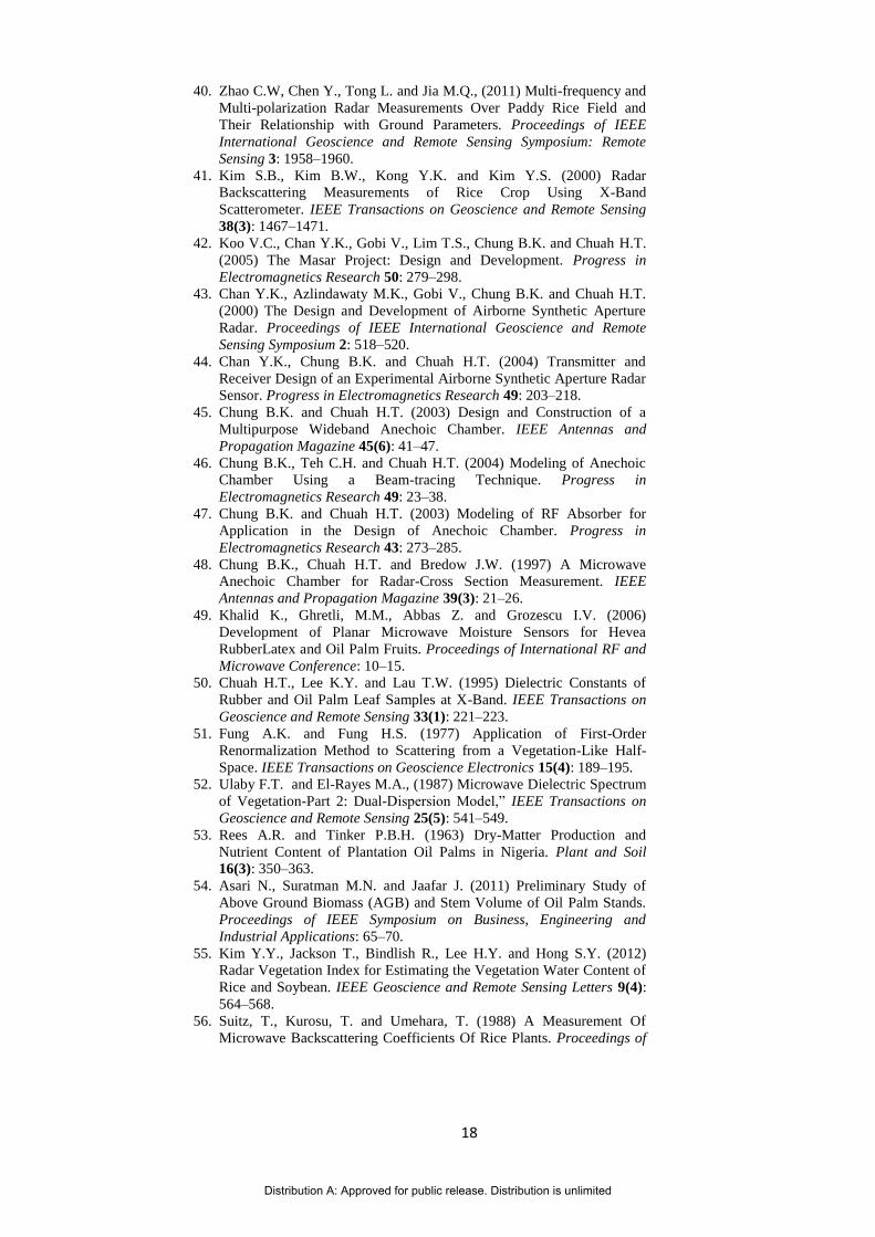
18

40. Zhao C.W, Chen Y., Tong L. and Jia M.Q., (2011) Multi-frequency and

Multi-polarization Radar Measurements Over Paddy Rice Field and

Their Relationship with Ground Parameters. Proceedings of IEEE


Sensing 3: 1958–1960.

41. Kim S.B., Kim B.W., Kong Y.K. and Kim Y.S. (2000) Radar

Backscattering Measurements of Rice Crop Using X-Band

Scatterometer. IEEE Transactions on Geoscience and Remote Sensing

38(3): 1467–1471.

42. Koo V.C., Chan Y.K., Gobi V., Lim T.S., Chung B.K. and Chuah H.T.

(2005) The Masar Project: Design and Development. Progress in

Electromagnetics Research 50: 279–298.

43. Chan Y.K., Azlindawaty M.K., Gobi V., Chung B.K. and Chuah H.T.

(2000) The Design and Development of Airborne Synthetic Aperture

Radar. Proceedings of IEEE International Geoscience and Remote


44. Chan Y.K., Chung B.K. and Chuah H.T. (2004) Transmitter and

Receiver Design of an Experimental Airborne Synthetic Aperture Radar

Sensor. Progress in Electromagnetics Research 49: 203–218.

45. Chung B.K. and Chuah H.T. (2003) Design and Construction of a

Multipurpose Wideband Anechoic Chamber. IEEE Antennas and

Propagation Magazine 45(6): 41–47.

46. Chung B.K., Teh C.H. and Chuah H.T. (2004) Modeling of Anechoic

Chamber Using a Beam-tracing Technique. Progress in


47. Chung B.K. and Chuah H.T. (2003) Modeling of RF Absorber for

Application in the Design of Anechoic Chamber. Progress in


48. Chung B.K., Chuah H.T. and Bredow J.W. (1997) A Microwave

Anechoic Chamber for Radar-Cross Section Measurement. IEEE

Antennas and Propagation Magazine 39(3): 21–26.

49. Khalid K., Ghretli, M.M., Abbas Z. and Grozescu I.V. (2006)

Development of Planar Microwave Moisture Sensors for Hevea

RubberLatex and Oil Palm Fruits. Proceedings of International RF and

Microwave Conference: 10–15.

50. Chuah H.T., Lee K.Y. and Lau T.W. (1995) Dielectric Constants of

Rubber and Oil Palm Leaf Samples at X-Band. IEEE Transactions on


51. Fung A.K. and Fung H.S. (1977) Application of First-Order

Renormalization Method to Scattering from a Vegetation-Like Half-

Space. IEEE Transactions on Geoscience Electronics 15(4): 189–195.

52. Ulaby F.T. and El-Rayes M.A., (1987) Microwave Dielectric Spectrum

of Vegetation-Part 2: Dual-Dispersion Model,” IEEE Transactions on


53. Rees A.R. and Tinker P.B.H. (1963) Dry-Matter Production and

Nutrient Content of Plantation Oil Palms in Nigeria. Plant and Soil

16(3): 350–363.

54. Asari N., Suratman M.N. and Jaafar J. (2011) Preliminary Study of

Above Ground Biomass (AGB) and Stem Volume of Oil Palm Stands.

Proceedings of IEEE Symposium on Business, Engineering and

Industrial Applications: 65–70.

55. Kim Y.Y., Jackson T., Bindlish R., Lee H.Y. and Hong S.Y. (2012)

Radar Vegetation Index for Estimating the Vegetation Water Content of

Rice and Soybean. IEEE Geoscience and Remote Sensing Letters 9(4):

564–568.

56. Suitz, T., Kurosu, T. and Umehara, T. (1988) A Measurement Of

Microwave Backscattering Coefficients Of Rice Plants. Proceedings of


19

IEEE International Geoscience and Remote Sensing Symposium 3:

1283–1286.

57. Yang C.J., Zhou J.M., Huang H. and Chen X. (2007) Correlations of the

Biomass of the Main Topical Forest Vegetation Types and LANDSAT

TM Data in Xishuangbanna of P. R. of China. Proceedings of IEEE

International Geoscience and Remote Sensing Symposium: 4336–4338.

58. Ouchi K. and Ipor I.B. (2002) Comparison of SAR and Optical Images

of the Rainforests of Borneo, Malaysia with Field Data. Proceedings of

IEEE International Geoscience and Remote Sensing Symposium 5:

2905–2907.

59. Zhao X.Y, Yang S.B., Shen S.H. and Li B.B. (2011) Assessment of

ENVISAT ASAR Data for Rice Monitoring Based on Three Years

Experiments. Proceedings of IEEE International Conference on Remote

Sensing, Environment and Transportation Engineering: 136–139.

60. Yamada Y. (2003) Relation between Ground Features and

Mathematical Morphology Using JERS-1/SAR Data During Flooding

Time in Paddy Areas. Proceedings of IEEE International Geoscience

and Remote Sensing Symposium 4: 2526–2528.

61. Paudyal D.R., Eiumnoh A. and Aschbacher J. (1995) Multitemporal

Analysis of SAR Images Over the Tropics for Agricultural Applications.


Symposium 2: 1219–1221.

62. Hung L.Q. and Batelaan O. (2003) Environmental Geological Remote

Sensing and GIS Analysis of Tropical Karst Areas in Vietnam.


Symposium 4: 2964–2966.

63. Malingreau J.P., De Grandi G.F., Leysen M., Mayaux P. and Simard M.

(1997) The ERS-1 Central Africa Mosaic: A New Role for Radar

Remote Sensing in Global Studies of the Tropical Ecosystem.


Symposium 4: 1725–1727.

64. Foody G.A. and Cutler M.E. (2002) Remote Sensing of Biodiversity:

Using Neural Networks to Estimate the Diversity and Composition of a

Bornean Tropical Rainforest from Landsat TM Data. Proceedings of

IEEE International Geoscience and Remote Sensing Symposium 1: 497–

499.

65. Marrufo L., Gonzalez F., Monsivais-Huertero A. And Ramos J. (2011)

Spatio-Temporal Estimation of Soil Moisture in a Tropical Region

using a Remote Sensing Algorithm. Proceedings of IEEE International

Geoscience and Remote Sensing Symposium: 3089–3092.

66. Yang C.J., Liu J.Y., Zhang Z.X. and Zhang Z.K. (2001) Estimation of

the Carbon Stock of Tropical Forest Vegetation by Using Remote

Sensing and GIS. Proceedings of IEEE International Geoscience and

Remote Sensing Symposium 4: 1672–1674.

67. Williams M.L., Milne T., Tapley I., Reis J.J., Sanford M., Kofman B.

and Hensley S. (2009) Tropical Forest Biomass Recovery Using

GeoSAR Observations. Proceedings of IEEE International Geoscience

and Remote Sensing Symposium 4: 173–176.


20

Appendix 2:

Development of Theoretical Model for Microwave Remote Sensing with

Computational Electromagnetics

Stage 1:

In order to understand how basic and important scatterers in the medium contribute

to the dominant scattering mechanisms that leads to final radar bacskattering returns

received by the satellite, it is decided that:

as currently the scattering matrices of basic shapes (disks, needles,

cylinders, ellipsoids) used by remote sensing models do not represent real

shapes and dimensions of actual components of scatterers in the natural

medium, EPA (Equivalence Principle Algorithm) is used to construct

scattering matrices of natural scatterers (modelled after real natural

objects such as tree trunk, branches, paddy leaf), and

backscattering returns from a layer of terrain (such as paddy field, oil

palm, dense vegetation) will be simulated through 2nd order iterative

Radiative Transfer Theory Solution with derived scattering matrices from

EPA and physical parameters from ground truth measurement, and

comparison of simulation results and satellite SAR images will be

conducted to determine the validity of model as well as analysis of key

scatterers and salient scattering mechanisms involved

Stage 2:

With the evaluation of model developed in Stage 1, development efforts in Stage 2

will focus on:

extension to multiscale modeling of clusters or configuration of natural

objects (like a layer of vegetation, paddy field etc) with new model

developed based on full EPA solution and direct simulation of scattered

fields through the EPA model developed, and

utilization of fast multipole algorithm in solution performance

improvement, and

analysis of simulation results and comparison and validation with satellite

SAR data


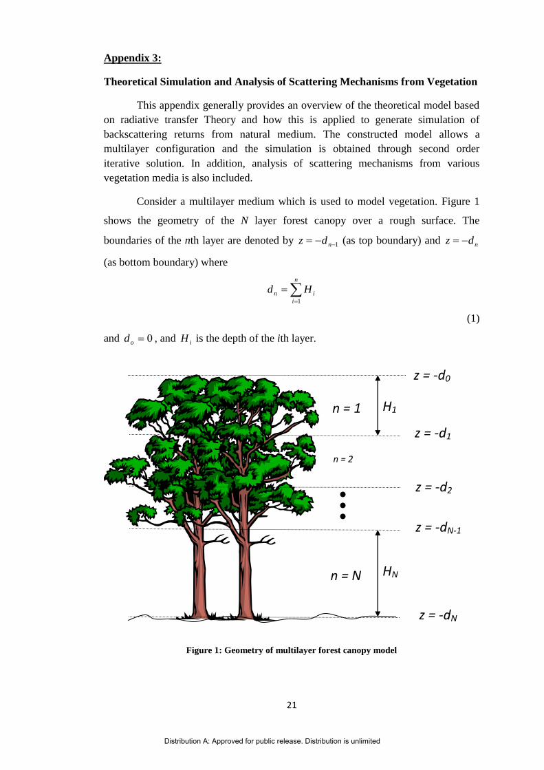
21

Appendix 3:

Theoretical Simulation and Analysis of Scattering Mechanisms from Vegetation

This appendix generally provides an overview of the theoretical model based

on radiative transfer Theory and how this is applied to generate simulation of

backscattering returns from natural medium. The constructed model allows a

multilayer configuration and the simulation is obtained through second order

iterative solution. In addition, analysis of scattering mechanisms from various

vegetation media is also included.

Consider a multilayer medium which is used to model vegetation. Figure 1

shows the geometry of the N layer forest canopy over a rough surface. The

boundaries of the nth layer are denoted by 1 ndz (as top boundary) and ndz

(as bottom boundary) where

n

i

in Hd1

(1)

and 0od , and iH is the depth of the ith layer.

Figure 1: Geometry of multilayer forest canopy model

n = 1

n = 2

n = N

H1

HN

z = -d0

z = -d1

z = -d2

z = -dN-1

z = -dN


22

In order to find the backscattering returns from the multilayer medium

described above, we can solve the radiative transfer equation shown in (2) below:

dIPIdz

Idecos

(2)

where I is the Stokes vector, e and P are the extinction matrix and phase matrix

of the medium, respectively. The phase matrix P for scatterers can be from

scatterers of basic shapes such as disk-shaped, needle-shaped, cylindrical and

ellipsoidal scatterers.

The radiative transfer equation is solved iteratively by using the albedo as an

iteration parameter. The phase matrices of these scatterers have included the

DMPACT (Dense Medium Phase and Amplitude Correction Theory) with array

phase correction factor and Fresnel amplitude and phase correction for coherence and

near field consideration. These are incorporated into the radiative transfer

formulation and up to second order solutions are obtained.

After solving for the intensity of the backscattered waves in the radiative transfer

equation, the backscattering coefficient can be obtained using this equation:-

iq

sps

pqI

I

cos4 (3)

where p and q represent the incident and backscattered polarizations respectively and

can be v or h. θs is the angle of the scattered field with respect to the normal of the

medium. Isp is the intensity of the backscattered waves, while Iiq is the intensity of the

incident wave.

The phase matrix of the scatterers in (2) is given by


23

hhhv

vhvv

hhhv

vhvv

nn PP

PP

SS

SSSP

22

(4)

where n

2 is the array phase correction factor. S is the phase matrix of a unit

volume of scatterers of a single class and it is obtained by averaging the Stokes

matrix over the size and spatial orientation of the scatterers.

)',';,(),,,,,()',';,( ScbapddddcdbdaP

(5)

where )',';,( S is the Stokes matrix that relates the scattered intensity of a

scatterer to the incident intensity. For ellipsoidal scatterer, a, b and c are the length of

the semi-major axes, and , and are the Eulerian angles which describe the

orientation of the ellipsoid. ),,,,,( cbap is the joint probability density function

for the quantities a, b, c, , and . The Stoke matrix has been improved to

include Fresnel amplitude and phase correction to consider the near field effect of the

scatterers. For detailed formulation of Fresnel correction, please refer to [1-2].

The array phase correction factor in (4) is given by

2

3 3

2 23

2 2

1

1

4

2 2 2 2

n

k k

si

q

si

x y z

q

e

d

e

d

k

q q

l

d

k l

qa k a k a k

si si

( )

!exp ( ) ( ) ( )

(6)

where

a kq

l

d

k l

qerf

qd l jk l

qr

r r( ) exp Re

( / )

2 2

4 2 and

ik and sk are the propagation vectors in the incident and scattering directions, l is

the array correlation length, d denotes the average distance between scatterers and

is the standard deviation of scatterers from their mean positions.


24

When we assume independent scattering from the scatterers, n

2 reduces to on ,

which is the number of scatterers per unit volume.

For a medium with N classes of scatterers, the total phase matrix is given by

N

i

itotal PP1

)',';,()',';,( .

(7)

The contribution of the solution of the radiative transfer equation can be expressed

by

210

spqspqspq

total

spq IIII

(8)

where w

spqI is the backscatter intensity with pq polarization (p,q = v,h) and w denotes

the order of the iterative solution of the radiative transfer equation. The components

of all these can be further divided to:

N

n

n

m

vv

spq

vv

spq

N

n

spq

vs

spq

v

spq

N

n

spq

s

spqspq

mnInII

snInII

II

2

1

11

2

1

1

0

)()(

)()(

(9)

where s

spqI is the contribution from the ground surface scattering and )(nI v

pq

accounts for direct volume scattering from the scatterers in nth layer. )( snI vs

pq

includes the interaction between the scatterers in the nth layer and the ground surface

(surface-volume scattering). )(nI vv

pq

and )( mnI vv

pq are the contributions from the

volume-volume scattering between the scatterers within the nth layer and between

the scatterers in layers n and m, respectively.


25

Regrouping the contribution terms in equation (9) into the surface, surface-

volume and volume scattering groups, the solution is then given by

v

spq

vs

spq

s

spq

total

spq IIII

(10)

N

n

n

m

vv

spq

vv

spq

N

n

v

spq

N

n

v

spq

vs

spq

vs

spq

mnInInII

snII

2

1

111

)()()(

)(

(11)

For detailed formulation of the steps mentioned above and details of

application of this model in natural medium such as paddy field and sea ice, please

refer to [3-6].

Table 1 lists the parameters used in the physical configuration of various

types of forest [Fig 1-2] which can be used by the model to study backscattering

returns and analyze dominant scattering mechanisms.

Temperate

Coniferous

Forest

Tropical

Deciduous

Forest

Tropical

Evergreen

Forest

Crown layer

(m)

5.50 3.00 6.00

Trunk layer (m) 4.00 1.50 2.00

Leaf:

Diameter (cm) 0.20 3.50 4.00

Length or

thickness (cm)

10.00 0.05 0.05

Density (#/m3) 1500 900 2600

Branch:

Diameter (cm) 1.00 2.50 3.00

Length (m) 1.50 1.50 2.00

Density (#/m3) 2.00 0.80 4.00

Upper Trunk:

Diameter (cm) 8.0 5.0 5.5

Length (m) 5.50 3.00 6.00

Density (#/m3) 0.0182 0.0666 0.1000

Lower Trunk:

Diameter (cm) 16.0 10.0 11.0

Length (m) 4.00 1.50 2.00

Density (#/m2) 0.0250 0.1333 0.3000

Table 1: Geometrical parameters for three types of forests.


26

Figure 1: Modelling of temperate coniferous forest as a two layer random medium with needles as

leaves.

Crown Layer

Trunk Layer

Figure 2: Modelling of tropical deciduous and evergreen forests as a two layer random medium with

circular disks as leaves.

Crown Layer

Trunk Layer


27

From the solutions, the following scattering contributions can be identified:

(i) Ground surface backscattering

(ii) Surface-volume scattering: leaf-ground, branch-ground, upper trunk-

ground and lower trunk-ground

(iii) Direct volume scattering: leaves, branches, upper trunks and lower

trunks

(iv) Volume-volume scattering (within the layer and between the layers)

Analysis of backscattering coefficient from different types of forests and vegetation

is provided below based on theoretical simulations from the model by the research

team over the years. This provides a good reference model for further development

of EPA based microwave remote sensing model.

(a) Temperate Coniferous Forest

Figure 3: VV backscattering coefficient of temperate coniferous forest at P band plotted against

incident angle for various dominant scattering mechanisms.

-30

-25

-20

-15

-10

-5

0

5

10

0 20 40 60 80

VV (Total)VV (Surface)VV (S-V, Upper Trunk)VV (V, Upper Trunk)VV (S-V, Lower Trunk)VV (Volume-Volume)

Bac

ksca

tterin

g C

oeffi

cien

t (dB

)

Incident Angle (degree)


28

Figure 3 to Figure 5 show the backscattering coefficient at P band (0.5 GHz)

for the coniferous forest plotted against the incident angle for VV, HH and VH

polarizations, respectively. In Figure 3 where the VV polarization case is shown, it

can be seen that at low incident angle ( i 50o), the dominant scattering

contribution comes from the surface-volume interactions between the ground surface

and the upper trunk. In addition, the lower trunk-ground interaction is also

considerably more important than other volume scattering contributions. In this case,

both the upper and the lower trunks act as corner reflectors to give strong scattering

in the backscattering direction. Direct backscattering from the ground surface is also

found important but decreases as the incident angle increases. For higher incident

angles ( i 50o), the surface-volume scattering contributions for VV polarization

become smaller in the region of angles where the Brewster angle effect is important.

At these high angles, it is found that the volume scattering from the upper trunk and

volume-volume scattering become dominant.


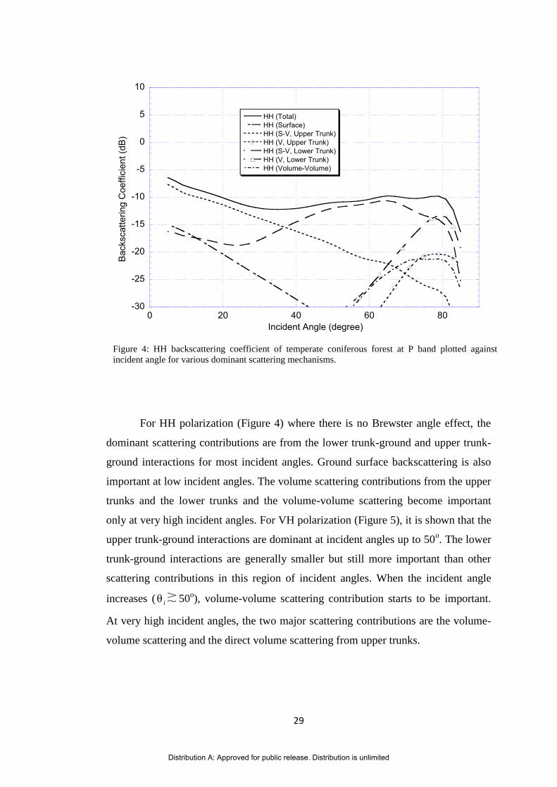
29

For HH polarization (Figure 4) where there is no Brewster angle effect, the

dominant scattering contributions are from the lower trunk-ground and upper trunk-

ground interactions for most incident angles. Ground surface backscattering is also

important at low incident angles. The volume scattering contributions from the upper

trunks and the lower trunks and the volume-volume scattering become important

only at very high incident angles. For VH polarization (Figure 5), it is shown that the

upper trunk-ground interactions are dominant at incident angles up to 50o. The lower

trunk-ground interactions are generally smaller but still more important than other

scattering contributions in this region of incident angles. When the incident angle

increases ( i 50o), volume-volume scattering contribution starts to be important.

At very high incident angles, the two major scattering contributions are the volume-

volume scattering and the direct volume scattering from upper trunks.

Figure 4: HH backscattering coefficient of temperate coniferous forest at P band plotted against


-30

-25

-20

-15

-10

-5

0

5

10

0 20 40 60 80

HH (Total)HH (Surface)HH (S-V, Upper Trunk)HH (V, Upper Trunk)HH (S-V, Lower Trunk)HH (V, Lower Trunk)HH (Volume-Volume)

Bac

ksca

tterin

g C

oeffi

cien

t (dB

)



30

At 10 GHz (X band), different scattering mechanisms are dominant for

backscattering from the coniferous forest considered. Figure 6 to Figure 8 show the

contributions from different scattering mechanisms against incident angles for VV,

HH and VH polarizations, respectively. At this frequency, due to the increase of

attenuation in the crown layer, the ground surface backscattering contributions and

the surface-volume scattering contributions are negligibly small. For VV polarization

(Figure 6), the needle-shaped leaves are the strongest scatterers compared with the

direct volume scattering from branches and trunks. For the range of incident angles

considered, the direct scattering from the needle-shaped leaves is dominant at low

incident angles whereas for most high incident angles, the volume-volume scattering

is more important. For HH polarization, the same observation as in the VV case can

be obtained. For VH polarization, it is found that the volume-volume scattering is the

strongest source in contributing the backscattering returns for most incident angles.

Although the direct volume scattering contribution from the leaves is smaller than

Figure 5: VH backscattering coefficient of temperate coniferous forest at P band plotted against


-40

-30

-20

-10

0

10

0 20 40 60 80

VH (Total)

VH (S-V, Upper Trunk)

VH (V, Upper Trunk)

VH (S-V, Lower Trunk)

VH (Volume-Volume)

Bac

ksca

tterin

g C

oeffi

cien

t (dB

)


Figure 6: VV backscattering coefficient of temperate coniferous forest at X band plotted against


-30

-25

-20

-15

-10

-5

0

5

10

0 20 40 60 80

VV (Total)

VV (V, Leaf)

VV (V, Branch)

VV (V, Upper Trunk)

VV (Volume-Volume)

Bac

ksca

tterin

g C

oeffi

cien

t (dB

)



31

that of the volume-volume scattering, it is much higher than the direct volume

scattering contribution from the branches.


32

Figure 7: HH backscattering coefficient of temperate coniferous forest at X band plotted against


-30

-25

-20

-15

-10

-5

0

5

10

0 20 40 60 80

HH (Total)

HH (V, Leaf)

HH (V, Branch)

HH (V, Upper Trunk)

HH (Volume-Volume)

Bac

ksca

tterin

g C

oeffi

cien

t (dB

)


Figure 8: VH backscattering coefficient of temperate coniferous forest at X band plotted against


-40

-30

-20

-10

0

10

0 20 40 60 80

VH (Total)

VH (V, Leaf)

VH (V, Branch)

VH (Volume-Volume)

Bac

ksca

tterin

g C

oeffi

cien

t (dB

)



33

(b) Tropical Deciduous Forest

For the tropical deciduous forest considered here, it has thicker branches and

smaller trunks compared with the temperate coniferous forest. From Figure 9 to

Figure 11 they show the various scattering contributions for a range of incident

angles for VV, HH and VH polarizations, respectively. For VV polarization (Figure

5.58), it is found that at low incident angles ( i 20o), the three dominant scattering

contributions are (in order of contribution) the ground surface backscattering, the

lower trunk-ground scattering and the direct volume scattering from the randomly

oriented branches. For incident angles between 20o and 50

o, the dominant scattering

contributions are from the direct volume scattering from the branches, the upper

trunk-ground interactions and the lower trunk-ground interactions. Combining the

two types of trunk-ground interactions, its contribution is still generally higher than

the direct volume scattering from the branches. For higher incident angles ( i 50o),

Figure 9: VV backscattering coefficient of tropical deciduous forest at P band plotted against incident

angle for various dominant scattering mechanisms.

-30

-25

-20

-15

-10

-5

0

0 20 40 60 80

VV (Total)VV (Surface)VV (V, Branch)VV (S-V, Upper Trunk)VV (V, Upper Trunk)VV (S-V, Lower Trunk)VV (Volume-Volume)

Bac

ksca

tterin

g C

oeffi

cien

t (dB

)



34

volume-volume scattering and direct volume scattering from the branches and upper

trunks are the dominant scattering mechanisms. As in the temperate coniferous case,

the Brewster angle effect reduces the volume-ground interactions at these high

incident angles.

For HH polarization (Figure 10), the lower trunk-ground interactions are

dominant over most incident angles, except at very low incident angles ( i 10o)

where ground surface backscattering is slightly more important. The direct volume

scattering from the branches and the branch-ground and the upper trunk-ground

interactions are also contributing substantially. For VH polarization (Figure 11), it is

clearly shown that the lower trunk-ground scattering contribution is important at low

incident angles ( i 30o) whereas the direct volume scattering from the branches is

dominant for higher incident angles.

Figure 10: HH backscattering coefficient of tropical deciduous forest at P band plotted against


-30

-25

-20

-15

-10

-5

0

0 20 40 60 80

HH (Total)HH (Surface)HH (S-V, Branch)HH (V, Branch)HH (S-V, Upper Trunk)HH (S-V, Lower Trunk)

Bac

ksca

tterin

g C

oeffi

cien

t (dB

)



35

At 10 GHz (X band), the various scattering contributions for the tropical

deciduous forest for VV, HH and VH polarizations are shown in Figure 12 to Figure

14, respectively. For both VV and HH polarizations (as shown in Figures 12 and 13),

it is clearly shown that the backscattering returns are generally dominated by the

direct volume scattering from the disk-shaped leaves and the volume-volume

scattering, where the former is more important than the latter at low incident angles

and vice versa at high incident angles. The other two scattering contributions that are

lower but may be considered are the direct volume scattering from the branches and

the upper trunks. The attenuation of the waves in the crown layer is high enough that

practically the volume scattering from the lower layer and the surface-volume

scattering contributions are negligibly small. For VH polarization (Figure 14), it is

found that the backscattering returns are solely from the volume-volume scattering as

the direct volume scattering from the disk-shaped leaves and branches and the leaf-

ground interactions do not contribute enough to be comparable to that of the volume-

volume scattering. The disk-shaped leaves with broad leaf surface in this case do not

Figure 11: VH backscattering coefficient of tropical deciduous forest at P band plotted against


-40

-35

-30

-25

-20

-15

-10

-5

0

0 20 40 60 80

VH (Total)VH (S-V, Branch)VH (V, Branch)VH (S-V, Upper Trunk)VH (S-V, Lower Trunk)VH (Volume-Volume)

Bac

ksca

tterin

g C

oeffi

cien

t (dB

)



36

produce as much cross polarized returns as the needle-shaped leaves in the temperate

coniferous case although both of them have almost the same volume fraction

(~0.04%).

Figure 12: VV backscattering coefficient of tropical deciduous forest at X band plotted against


-30

-25

-20

-15

-10

-5

0

0 20 40 60 80

VV (Total)VV (V, Leaf)VV (V, Branch)VV (V, Upper Trunk)VV (Volume-Volume)

Bac

ksca

tterin

g C

oeffi

cien

t (dB

)



37

Figure 13: HH backscattering coefficient of tropical deciduous forest at X band plotted against


-30

-25

-20

-15

-10

-5

0

0 20 40 60 80

HH (Total)HH (V, Leaf)HH (V, Branch)HH (V, Upper Trunk)HH (Volume-Volume)

Bac

ksca

tterin

g C

oeffi

cien

t (dB

)


Figure 14: VH backscattering coefficient of tropical deciduous forest at X band plotted against


-40

-35

-30

-25

-20

-15

-10

-5

0

0 20 40 60 80

VH (Total)VH (S-V, Leaf)VH (V, Leaf)VH (V, Branch)VH (Volume-Volume)

Bac

ksca

tterin

g C

oeffi

cien

t (dB

)



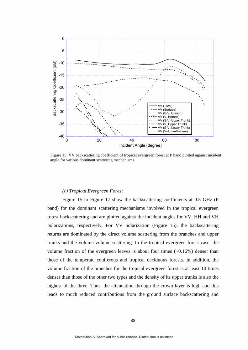
38

(c) Tropical Evergreen Forest

Figure 15 to Figure 17 show the backscattering coefficients at 0.5 GHz (P

band) for the dominant scattering mechanisms involved in the tropical evergreen

forest backscattering and are plotted against the incident angles for VV, HH and VH

polarizations, respectively. For VV polarization (Figure 15), the backscattering

returns are dominated by the direct volume scattering from the branches and upper

trunks and the volume-volume scattering. In the tropical evergreen forest case, the

volume fraction of the evergreen leaves is about four times (~0.16%) denser than

those of the temperate coniferous and tropical deciduous forests. In addition, the

volume fraction of the branches for the tropical evergreen forest is at least 10 times

denser than those of the other two types and the density of its upper trunks is also the

highest of the three. Thus, the attenuation through the crown layer is high and this

leads to much reduced contributions from the ground surface backscattering and

Figure 15: VV backscattering coefficient of tropical evergreen forest at P band plotted against incident


-40

-35

-30

-25

-20

-15

-10

-5

0

0 20 40 60 80

VV (Total)VV (Surface)VV (S-V, Branch)VV (V, Branch)VV (S-V, Upper Trunk)VV (V, Upper Trunk)VV (S-V, Lower Trunk)VV (Volume-Volume)

Bac

ksca

tterin

g C

oeffi

cien

t (dB

)



39

surface-volume scattering as compared to direct volume scattering and volume-

volume scattering from the crown layer. For VV polarization as shown in Figure 15,

direct volume scattering contribution from the branches is dominant for most

incident angles, except at high incident angles ( i 60o) where the direct volume

scattering contribution from the upper trunks becomes equally important. Due to its

smaller size compared to the branches and upper trunks, the disk-shaped leaves

contribute relatively less backscattering returns.

For HH polarization (Figure 16), the backscattering contribution from the

branches is dominant for the range of incident angles considered here. It can be seen

that those surface-volume contributions (branches and trunks) are generally more

important than in the VV polarization case for wider incident angle range as there is

no Brewster angle effect for HH polarization. In Figure 17 where the VH

polarization case is shown, the direct volume scattering from the branches and

Figure 16: HH backscattering coefficient of tropical evergreen forest at P band plotted against incident


-40

-35

-30

-25

-20

-15

-10

-5

0

0 20 40 60 80

HH (Total)HH (Surface)HH (S-V, Branch)HH (V, Branch)HH (S-V, Upper Trunk)HH (V, Upper Trunk)HH (S-V, Lower Trunk)HH (Volume-Volume)

Bac

ksca

tterin

g C

oeffi

cien

t (dB

)



40

volume-volume scattering are important contributors to the backscattering returns

throughout the range of incident angles considered.

At 10 GHz (X band), similar plots for the VV, HH and VH polarizations are

shown in Figure 18 to Figure 20. For VV and HH polarizations, it is found that the

leaves are the dominant scatterers for incident angles less than 20o. For higher

incident angles, the volume-volume scattering becomes more important than other

scattering mechanisms. For VH polarization, as in the case of tropical deciduous

forest, the backscattering returns are significantly due to the volume-volume

scattering.

Figure 17: VH backscattering coefficient of tropical evergreen forest at P band plotted against incident


-50

-40

-30

-20

-10

0

0 20 40 60 80

VH (Total)VH (S-V, Branch)VH (V, Branch)VH (S-V, Upper Trunk)VH (V, Upper Trunk)VH (S-V, Lower Trunk)VH (Volume-Volume)

Bac

ksca

tterin

g C

oeffi

cien

t (dB

)



41

Figure 19: HH backscattering coefficient of tropical evergreen forest at X band plotted against


-30

-25

-20

-15

-10

-5

0

0 20 40 60 80

HH (Total)HH (V, Leaf)HH (V, Branch)HH (V, Upper Trunk)HH (Volume-Volume)

Bac

ksca

tterin

g C

oeffi

cien

t (dB

)


Figure 18: VV backscattering coefficient of tropical evergreen forest at X band plotted against


-30

-25

-20

-15

-10

-5

0

0 20 40 60 80

VV (Total)VV (V, Leaf)VV (V, Branch)VV (V, Upper Trunk)VV (Volume-Volume)

Bac

ksca

tterin

g C

oeffi

cien

t (dB

)



42

Figure 20: VH backscattering coefficient of tropical evergreen forest at X band plotted against


-40

-35

-30

-25

-20

-15

-10

-5

0

0 20 40 60 80

VH (Total)VH (V, Leaf)VH (V, Branch)VH (V, Upper Trunk)VH (Volume-Volume)

Bac

ksca

tterin

g C

oeffi

cien

t (dB

)



43

From the analysis above for the cases of 0.5 GHz and 10.0 GHz, it is known that the

dominance of certain scattering mechanisms changes with frequency. To show this effect in

more detail, the deciduous forest case is chosen and the backscattering coefficients for

various scattering mechanisms at 45o incident angle are plotted for a frequency range of 0.5

GHz to 10 GHz. Figure 21 to Figure 23 show the graphs for VV, HH and VH polarizations,

respectively. Only those dominant scattering mechanisms will be included in the graphs.

For VV polarization, it is found that at 0.5 GHz, three dominant scattering

mechanisms are the direct volume scattering from the branches, the upper trunk-ground

interactions and the lower trunk-ground interactions. When the frequency increases (~ 1 GHz

– 3 GHz), the dominant scattering mechanisms are the direct volume scattering from the

branches and upper trunks and the volume-volume scattering. For higher frequency ( 3

GHz), volume-volume scattering becomes the dominant scattering mechanism, but the other

important contributors to the backscattering returns are the direct volume scattering from the

leaves, branches and upper trunks. It should be noted that the direct scattering contribution

from the leaves increases as the frequency increases and becomes the most important direct

Figure 21: VV backscattering coefficient of tropical deciduous forest at 45o incident angle plotted

against frequency for various dominant scattering mechanisms.

-40

-30

-20

-10

0

10

0 2 4 6 8 10

VV (Total)VV (V, Leaf)VV (V, Branch)VV (S-V, Upper Trunk)VV (V, Upper Trunk)VV (S-V, Lower Trunk)VV (Volume-Volume)

Bac

ksca

tterin

g C

oeffi

cien

t (dB

)

Frequency (GHz)


44

scattering mechanism at 5 GHz and above when compared with the direct scattering from the

other scatterers such as the branches and upper trunks.

Figure 22: HH backscattering coefficient of tropical deciduous forest at 45o incident angle plotted


-40

-30

-20

-10

0

10

0 2 4 6 8 10

HH (Total)HH (V, Leaf)HH (V, Branch)HH (V, Upper Trunk)HH (S-V, Lower Trunk)HH (Volume-Volume)

Bac

ksca

tterin

g C

oeffi

cien

t (dB

)

Frequency (GHz)


45

For HH polarization, the dominant scattering mechanism at 0.5 GHz is the trunk-

ground interaction from the lower trunks (which have diameter twice that of the upper trunks).

As frequency increases, the direct volume scattering from the branches becomes important

and the contribution from the lower-trunk interaction decreases. For frequency higher than 5

GHz, the same trend found in the VV polarization case is observed where the volume-volume

scattering becomes the dominant scattering mechanism and the direct volume scattering from

the leaves, branches and upper trunks are important. Out of the three direct volume scattering

contributions, the contribution from direct scattering from the leaves is the highest. For VH

polarization, the trend is simpler where the direct volume scattering from the branches is

important at low frequency ( 2 GHz) and decreases as frequency increases and the volume-

volume scattering dominates at high frequency ( 2 GHz).

(d) Paddy Field and Oil Palm

In Figure 24, it shows a plot of various scattering mechanisms involved in the C-band

HH backscattering coefficient of a 26-day old paddy field in Sungai Burung, Selangor State,

Figure 23: VH backscattering coefficient of tropical deciduous forest at 45o incident angle plotted


-40

-30

-20

-10

0

10

0 2 4 6 8 10

VH (Total)VH (V, Leaf)VH (S-V, Branch)VH (V, Branch)VH (S-V, Upper Trunk)VH (S-V, Lower Trunk)VH (Volume-Volume)

Bac

ksca

tterin

g C

oeffi

cien

t (dB

)

Frequency (GHz)


46

Malaysia where the ground truth measurement was conducted to collect physical parameters

to be input to the simulation program based on this model.

In Figure 25, various scattering mechanisms involved in HH backscattering

coefficient for two-year old oil palm is shown. Input physical parameters were obtained from

ground truth measurement conducted in Perak State, Malaysia in August, 2013.

Figure 24: Various scattering mechanisms (HH polarization) in paddy field.

-30

-25

-20

-15

-10

-5

0

0 20 40 60 80

surface-volume scatteringsingle volume scatteringdouble volume scatteringtotal scattering

Back

scat

terin

g C

oeffi

cien

t (dB

)

Angle (deg)


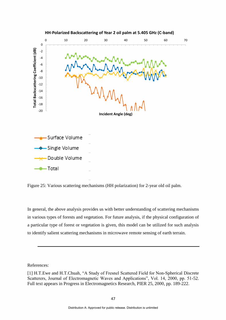
47

Figure 25: Various scattering mechanisms (HH polarization) for 2-year old oil palm.

In general, the above analysis provides us with better understanding of scattering mechanisms

in various types of forests and vegetation. For future analysis, if the physical configuration of

a particular type of forest or vegetation is given, this model can be utilized for such analysis

to identify salient scattering mechanisms in microwave remote sensing of earth terrain.

References:

[1] H.T.Ewe and H.T.Chuah, “A Study of Fresnel Scattered Field for Non-Spherical Discrete

Scatterers, Journal of Electromagnetic Waves and Applications”, Vol. 14, 2000, pp. 51-52.

Full text appears in Progress in Electromagnetics Research, PIER 25, 2000, pp. 189-222.

-20

-18

-16

-14

-12

-10

-8

-6

-4

-2

0

0 10 20 30 40 50 60 70

Tota

l Bac

ksca

tte

rin

g C

oe

ffic

ien

t (d

B)

Incident Angle (deg)

HH-Polarized Backscattering of Year 2 oil palm at 5.405 GHz (C-band)


48

[2] J.Y. Koay, H.T. Ewe and H.T. Chuah, “A Study of Fresnel Scattered Fields for

Ellipsoidal and Elliptic Disk-Shaped Scatterers,” IEEE Transactions on Geoscience and

Remote Sensing, Vol. 46, No. 3, 2008, pp. 1091 – 1103.

[3] H.T.Ewe and H.T.Chuah, “Electromagnetic Scattering from an Electrically Dense

Vegetation Medium”, IEEE Transactions on Geoscience and Remote Sensing, Vol. 38, No. 5,

2000, pp. 2093-2105.

[4] Chuah, H. T., Tjuatja, S., Fung, A. K. & Bredow, J. W. A phase matrix for a dense

discrete random medium: Evaluation of volume scattering coefficient. IEEE Transactions on

Geoscience and Remote Sensing, 34(5), 1996, pp. 1137-1143.

[5] J. Y. Koay, C. P. Tan, K. S. Lim, Saiful Bahari, H. T. Ewe, H. T. Chuah, J. A. Kong,

“Paddy Fields as Electrically Dense Media: Theoretical Modeling and Measurement

Comparisons with Season-Long Data,” IEEE Transactions on Geoscience and Remote

Sensing, Vol. 45, No. 9, 2007, pp. 2837-2849.

[6] M. D. Albert, Y. J. Lee, H.T. Ewe, and H.T. Chuah, “Multilayer Model Formulation and

Analysis of Radar Backscattering from Sea Ice,” Progress in Electromagnetics Research

(PIER), Vol. 128, 2012, pp. 267-290.


49

Appendix 4:

Pilot Ground Truth Measurement

In order to understand better the physical configuration of natural medium such as vegetation,

it is necessary for ground truth measurement to be conducted. The project team has

previously conducted detailed ground truth measurement in paddy (or rice, largely planted in

Asia region) field in Malaysia as well as sea ice and ice shelf areas in Ross Island Antarctica,

these collected data will be useful in the modeling work. In 2013, with the support of funding

of related project, detailed ground truth measurement of oil palm plantation was carried out.

As of 2006, 11,000,000 hectares (42,000 sq mi) of oil palm plantation are found in tropical

countries like Indonesia and Malaysia.

On 29 – 30 August 2013, ground truth measurement of oil palm trees was done at Changkat

Chermin Estate and Lekir Estate in Perak State, Malaysia. For pilot study, plantation plots for

2, 7 and 14 year old palm were chosen.

Parameters such as leaf length, leaf width, leaf thickness, frond radius, frond length, trunk

circumference and trunk height were measured. LaserAce TM 1000 rangefinder was used to

measure canopy height and trunk height of taller palm. In addition, number of leaves per

frond, number of fronds per palm and general distribution of leaf inclination angle were also

counted and observed.

Samples of leaf, frond and soil of each plantation plot were also collected for measurement of

moisture content and dielectric constant of each sample will then be calculated based on

empirical model published in the literature.

These ground truth measurement parameters will be used as input parameters of model

simulation.

Table 1 shows some of the physical parameters collected through the pilot ground truth

measurement.

Table 1: Physical parameters measured in oil palm plantation.

Age of oil palm Y2 Y7 Y14

Leaf length (cm) 72.5 83.5 98.5

Leaf width (cm) 2.5 4 4.5

No of leaves per frond 232 295 268

Frond radius (cm) 1.15 1.53 1.67

Frond length (cm) 316 626 645

No of fronds per palm 40 40 48

Canopy height (cm) 399 663 717Planting Density (palms/ha) 145 136 130Surface soils type Marine Clay Silt Clay Sandy Clay Loam


50

It was also noticed that the growth of 14-year oil palm plot selected was not well as it was

located at a site with soil type of sandy clay loam and number of leave per frond is less

compared with that of 7-year oil palm plot. Figures 1-2 are collection of photos taken during

the ground truth measurement. A more thorough field trip measurement was later conducted

in October, 2013.

Figure 1: Oil palm plots (2-year, 7-year and 14 year).

Figure 2: Measuring physical parameters of oil palm plots.


51

Appendix 5:

LOOP-TREE FREE AUGMENTED EQUIVALENCE PRINCIPLE

ALGORITHM FOR LOW FREQUENCY PROBLEMS

1. INTRODUCTION

Solving full-wave electromagnetic problems is challenging, especially when the structure is working at low

frequencies [1]. These problems are often encountered in ICs, electronic packaging, PCBs, small antennas, and

small sensors. Computational electromagnetics (CEM) research is crucial in accurately predicting the

electromagnetic behavior of this kind of structures.

A challenging problem in computational electromagnetics is the electrodynamics problem in the low

frequency regime. When the wavelength is much longer than the size of the structure, the physics of the

electromagnetic field resembles that of circuits. This is the circuit-physics regime. When the wavelength is

sizeable compared to the structure, wave physics becomes important. It is important for a simulation method to

capture proper physics at different frequency bands [2]. When a structure is multiscale, it has parts that are small

compared to wavelength, and parts that are on the order of wavelength. Hence, both circuit physics and wave

physics are equally important. A simulation method has to capture both physics to conquer this difficulty.

A popular way of solving these problems is to use integral equation (IE) methods [3]. Although the IE method

with the novel RWG basis [4] has been a prevalent solution to various electromagnetic problems, it does not

work well at low frequencies. This is due to the fact that the electric field and the magnetic field are weakly

coupled at the low frequency regime decomposing into inductance physics and capacitance physics. Hence,

most numerical methods working in mid frequencies do not capture both phenomena simultaneously, yielding

low-frequency breakdown. So far, some techniques have been proposed to handle this issue including the loop-

tree decomposition [5-7]. However, it is laborious to find the loop-tree basis for complicated structures. In [8],

an augmented electric field integral equation (A-EFIE) has been proposed to solve the low-frequency problem

without the need of loop-tree basis. In this method, the EFIE is augmented with an additional charge unknown,

and an additional continuity equation relating the charge to the current. The resultant equation, after proper

frequency normalization, is frequency stable down to very low frequency.

In the work of [9], the equivalence principle algorithm (EPA) has been used to capture the multi-scale physics

of complex structures by partitioning objects into parts through equivalence surfaces. The interaction of the

electromagnetic field between equivalence surfaces is done through translation operators and the equivalence

currents on equivalence surfaces. The solution within the equivalence surface can be obtained by various

numerical methods, which must be low frequency stable. To surmount the low frequency issue, [10] used the

augmented EPA that applies the similar idea of A-EFIE to separate the vector potential term and scalar potential

term. This method avoids ill conditioning at low frequencies. In this method, however, the solvers inside

equivalence surfaces employ the loop-tree basis, which becomes burdensome when it comes to the complex

structure. Hence, it is beneficial to develop an A-EPA method that is loop-tree free. In this project activity, we

developed a new A-EPA that is based on A-EFIE to avoid the loop-tree involvement. Several numerical

examples are provided to validate this proposed new method.

2. AUGMENTED EQUIVALENCE PRINCIPLE ALGORITHM

Based on the equivalence principle, the scattering of one object can be calculated in conjunction with an

equivalence surface (ES). It includes three steps: outside-in propagation, solving for the current on the object,

and inside-out propagation. First, the incident currents on the equivalence surface replace the source outside ES.

Next, the electric current on the object is solved by MoM solver. In the last step, the scattered electric and

magnetic field can be computed using the electric and magnetic currents on ES. This also can be described by

the equivalence principle operator [9] (we also denote it the scattering operator for short):

incsca S XX ~

(1)

where X is the unknown vector on ES

me

ssT

MJX

1 (2)


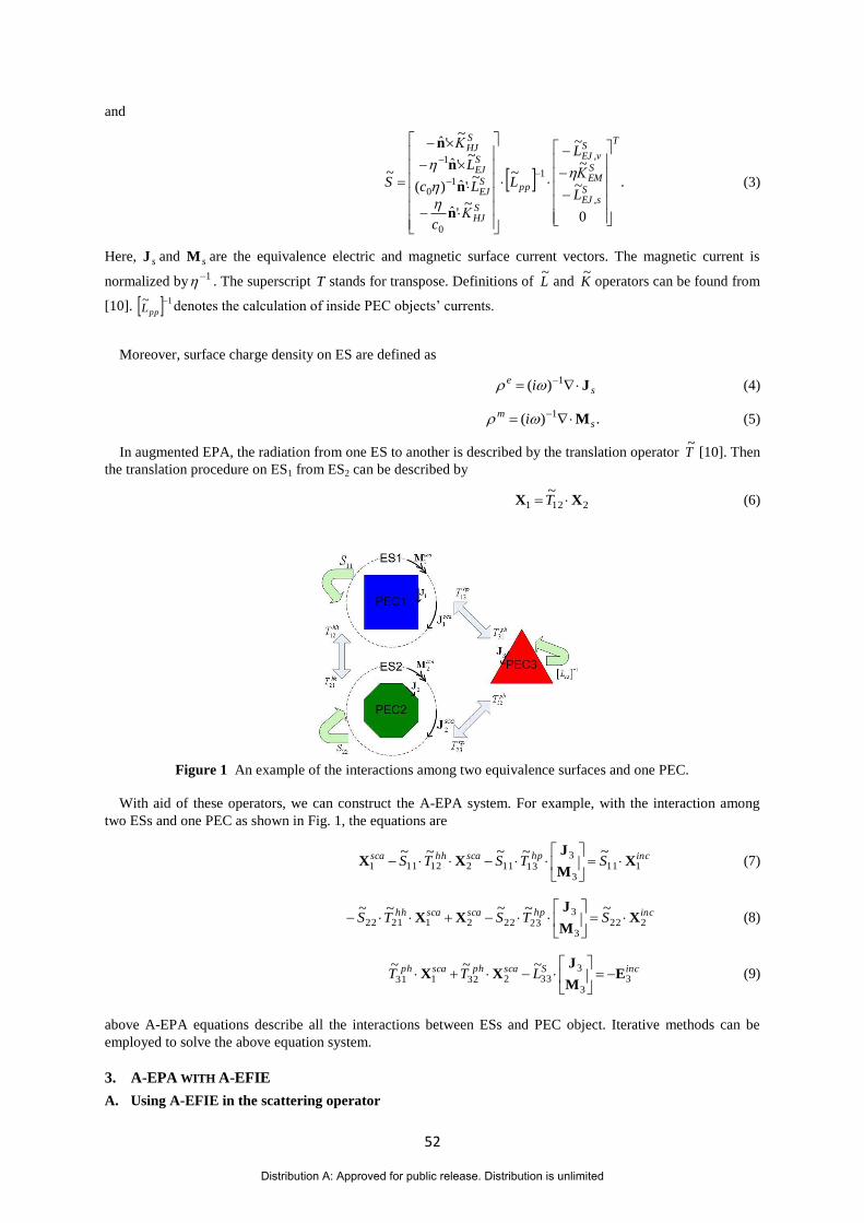
52

and

.

0

~

~

~

~

~'ˆ

~'ˆ)(

~'ˆ

~'ˆ

~

,

,

1

0

10

1

T

SsEJ

SEM

SvEJ

pp

SHJ

SEJ

SEJ

SHJ

L

Κ

L

L

Κc

Lc

L

Κ

S

n

n

n

n

(3)

Here, sJ and sM are the equivalence electric and magnetic surface current vectors. The magnetic current is

normalized by 1 . The superscript T stands for transpose. Definitions of L~

and K~

operators can be found from

[10]. 1~

ppL denotes the calculation of inside PEC objects’ currents.

Moreover, surface charge density on ES are defined as

se i J 1)( (4)

.)( 1s

m i M (5)

In augmented EPA, the radiation from one ES to another is described by the translation operator T~

[10]. Then

the translation procedure on ES1 from ES2 can be described by

2121

~XX T (6)

Figure 1 An example of the interactions among two equivalence surfaces and one PEC.

With aid of these operators, we can construct the A-EPA system. For example, with the interaction among

two ESs and one PEC as shown in Fig. 1, the equations are

inchpscahhsca STSTS 1113

31311212111

~~~~~X

M

JXX

(7)

inchpscascahh STSTS 2223

32322212122

~~~~~X

M

JXX

(8)

incSscaphscaphLTT 3

3

333232131

~~~E

M

JXX

(9)

above A-EPA equations describe all the interactions between ESs and PEC object. Iterative methods can be

employed to solve the above equation system.

3. A-EPA WITH A-EFIE

A. Using A-EFIE in the scattering operator


53

The augmented electric field integral equation (A-EFIE) [11] treats the charge as an unknown and introduces

an additional equation to relate the current and the charge. Similar to using both Kirchhoff's current and voltage

law (KCL and KVL) in Modified Nodal Analysis (MNA), it bypasses the imbalance between the vector

potential and the scalar potential in the conventional EFIE. Hence, the A-EFIE formulation includes not only the

current but also the charge as unknowns. It has a 22 block structure as:

0

1

0

0

20

bJ

ID

PDV

c

ik

k

T

(10)

where J is current density , is the vector of charge density, b is the excitation vector, and I is an identity

matrix. The sub-matrices are written as

nm S

nS

mrnm dSdSg ')'()',()(, rΛrrrΛV (11)

nm Sn

Smrnm dSdShgh ')'()',()(1

, rrrrP (12)

where Λ stands for the RWG basis function, h is the pulse expansion function, and )',( rrg is the Green's

function in the homogeneous medium. Here, D is a divergence operator and defined as

nm

nm

nm

nm

RWG ofpart negative theis path ,1

RWG ofpart positive theis path ,1

RWG tobelongnot does path ,0

,D (13)

The augmented EPA method has the capability to suppress the low-frequency breakdown of EPA method on

equivalence surfaces. But its L~

operator inside the equivalence surface still uses the loop-tree decomposition

technique to overcome the low frequency issues. It becomes complicated especially for complex structures. This

difficulty can be solved by using the A-EFIE method.

In this method, the S~

operator of A-EPA becomes

T

SsEJ

SEM

SvEJ

EFIEApp

SHJ

SEJ

SEJ

SHJ

L

Κ

L

L

Κc

Lc

L

Κ

S

0

~

~

~

~

~'ˆ

~'ˆ)(

~'ˆ

~'ˆ

~

,

,

1

0

10

1

n

n

n

n

(14)

where the 1~

EFIEAppL is the operator in Eq. (10). Assuming that one object (labeled as i) is enclosed in an

equivalent surface, the inside operator becomes:

.~

1

20

)(

)()(1)(

ID

PDV

kL

i

iTi

EFIEA

ipp (15)

B. Tap basis scheme

Decomposing a general structure into small-scale parts is challenging. In [12], a tap basis scheme has been

proposed to handle this difficulty. This scheme can be extended for solving low frequency problems.


54

Figure 2 A strip intersects with an equivalence surface.

As shown in Fig. 2, a metallic strip intersects with the equivalence surface. The currents on the strip are then

divided into three parts: inside current sJ , tap current tJ , and outside current pJ . Using the same technique of

[12], the A-EPA equation system becomes

inct

incp

incth

inc

t

p

tttp

ptppph

tthpth

hthp

S

S

LLI

LLT

STSI

STSI

E

E

X

X

Y

Y

t

X~

~

~~0

~~0

~

~~~0

~~~0

(16)

where Y refers to TJ , t is the tap vector

.~

stsL Yt (17)

4. NUMERICAL RESULTS

To demonstrate the accuracy and validity of the proposed method, we simulated several examples, including

both scattering and radiation problems. The platform we worked on is a computer with 2.67 GHz CPU, 12 GB

memory, and the Linux operating system.

In the first example, the scattering problem of a PEC sphere is calculated. The PEC sphere with a radius of

1.0 m is enclosed in a Huygens' box that has the edge length of 2.4 m. This sphere is illuminated by an x-

polarized plane wave from the z direction. Fig. 3(a) shows the RCS result solved by EPA with normal EFIE

while Fig. 3(b) demonstrates the corresponding result solved by A-EPA with A-EFIE. As can be seen from these

two figures, traditional EPA method fails to obtain the correct answer at 1 MHz whereas A-EPA with A-EFIE

can work well even at frequencies as low as 2 KHz.

Next, we use the proposed method to simulate a differential via-hole structure. Two coupled striplines start

from the upper layer, go through the via-holes to the second layer, and then return to the first layer. This

differential vias with holes are frequently encountered in integrated circuits. The geometry specifications are

shown in Fig. 4.

In order to alleviate the computational burden, two equivalent surfaces are employed. It shall be noted that

finding the loop-tree basis for this via-holes structure is laborious because it takes significant efforts to search

for global loops in the presence of holes. The proposed method circumvents this trouble by A-EFIE operator

method inside ESs.


55

(a)

(b)

Figure 3 Scattering of a unit sphere: (a) simulated by EPA with EFIE at 1MHz, (b) simulated by proposed method at 2KHz.

Figure 4 Differential vias structure: top view, side view and tracks only.

In this case, the via-hole structure is enclosed by two ESs as shown in Fig. 5. A delta feed port is imposed at

the middle of its left end. The calculated current distribution of this structure is showing in Fig. 6 where the

wavelength is 3.0 mm. The results are validated by normal MoM with A-EFIE.


56

As the third example, a metallic ball array is modeled and simulated. The coupling current distribution has

been analyzed when one of balls is excited by a delta source. 32 EPA boxes are created and used. Due to the

geometry similarity of all the balls, A-EPA with A-EFIE only one scattering operator is solved and reused for

coupling interactions. The current distribution is shown in Fig. 7 at the frequency of 300 MHz.

Figure 5 Two ESs enclose the via hole structure.

Figure 6 Current Distribution of via-hole structure.


57

Figure 7 Ball array analysis: top view, geometry specification and current distribution. Frequency is 300MHz. The center to center distance between neighboring balls is 4 mm. The diameter of each ball is 2 mm.

5. CONCLUSION

In this work, a new augmented EPA with augmented EFIE has been presented to solve low frequency domain

decomposition problems. The A-EPA applies equivalent surface electric and magnetic charges to bypass the low

frequency instability problem. With the incorporation of A-EFIE in the scattering operator, this method can be

used to solve low frequency problems without using loop-tree basis. From numerical verifications, the proposed

method is stable and effective in solving problems at low frequencies. Furthermore, this method can be further

integrated with fast multipole methods (FMM) to solve large-scale problems.

REFERENCES

1. W. C. Chew, L. Jiang, Y. Chu, G. Wang, L.-T. Chiang, Y. Pan, and J. Zhao, Toward a more robust and accurate CEM fast integral equation solver for IC applications, IEEE Trans Advanced Packaging 28(2005), 449–464.

2. W. C. Chew, Computational electromagnetics–the physics of smooth versus oscillatory fields, Philo. Trans. Royal Soc. London Series

A, Math., Phys. Eng. Sci., 362 (2004), 579–602. 3. R. F. Harrington, Field Computation by Moment Method, MacMillan, New York (1968).

4. S. Rao, D. Wilton, and A. Gllisson, Electromagnetic scattering by surfaces of arbitrary shape, IEEE Trans Antennas and Propagation

30 (1982), 409–418. 5. D. R. Wiltion and A. W. Glisson, On improving the electric field integral equation at low frequencies, In: Proceeding of the URSI

Radio Science Meeting Digest, Los Angeles, CA, USA, 1980, p. 24.

6. J. Mautz and R. Harrington, An E-field solution for a conducting surface small or comparable to the wavelength, IEEE Trans Antennas and Propagation 32 (1984), 330–339.

7. J.-S. Zhao and W. C. Chew, Integral equation solution of Maxwell's equations from zero frequency to microwave frequencies, IEEE

Trans Antennas and Propagation 48 (2000), 1635–1645. 8. Z.-G. Qian and W. C. Chew, A quantitative study on the low frequency breakdown of EFIE, Microwave Opt Technol Lett 50 (2008),

1159-1162.

9. M. K. Li, W. C. Chew and L. J. Jiang, A domain decomposition scheme based on equivalence theorem, Microwave Opt Technol Lett 48 (2008), 1159-1162.

10. L. E. Sun, W. C. Chew and J. M. Jin, Augmented equivalence principle algorithm at low frequencies, Microwave Opt Technol Lett 52

(2010), 2274-2279. 11. Z.-G. Qian and W. C. Chew, Fast full-wave surface integral equation solver for multiscale structure modeling, IEEE Trans Antennas

and Propagation 57 (2009), 3594–3601.

12. M.-K. Li and W. C. Chew, Multiscale simulation of complex structures using equivalence principle algorithm with high-order field point sampling scheme, IEEE Trans Antennas and Propagation 56 (2008), 2389–2397.


58

Appendix 6:

A Novel Broadband Equivalent Source Reconstruction Method for

Broadband Radiators

1 INTRODUCTION

Equivalent source reconstruction methods are widely employed as a near-field (NF) measurement post-

processing technique. With this equivalent source, antenna diagnostics, near-field to far-field transformations

(NF-FF), etc., can be easily performed. Moreover, source reconstruction is more flexible in handling complex

geometries where equivalent current source as well as the measurement domain reside. These merits are hard

to be observed in wave expansion methods [1].

The source reconstruction method (SRM) has received intensive attention for near-field far-field (NF-FF)

transformations. People firstly facilitate SRM by placing equivalent electric or magnetic current sources at an

infinite large planar perfect electric conductor (PEC) or magnetic conductor (PMC) [2]-[3]. The deficiency of

these methods is its difficulties in handling the whole 3-D radiation pattern. This problem was addressed in

[4] by constructing the equivalent current source over an surface enclosing the radiator or just the surface of

the radiator. The fast multipole algorithm is introduced in [5] to accelerate the matrix-vector product with the

purpose of tackling electrical large problems.

However, the equivalent sources built in these references are only mostly valid at a single frequency. Our

aim is to construct the equivalent source that is able to deal with wide-band problems without involving all

frequencies. With this wide-band model, the computational cost will be greatly reduced since we do not need

to invert or factorize

Figure 1: The inverse equivalent source reconstruction process and the NF-NF or NF-FF transformation process.

the matrix system at each frequency. To achieve our purpose, an efficient interpolation algorithm suitable

for our problem must be developed. In this work, the Neville-type Stoer-Bulirsch rational interpolation

algorithm is adopted [6]. The SB algorithm is derivative free. Thus, it is amenable to our problem. To

effectively reduce the number of samples, an adaptive frequency sampling strategy based on the bisection-

searching scheme allowing frequency step to be locally refined without limitation is employed.

In order to achieve high-order accuracy, high-order hierarchical basis can be used. But it will make the

problem very complex and increase the amount of computation required per entry of the system matrix.

Another easy and convenient alternative is the Nystrom method [7]. In the Nystrom method, the unknown

quantity is represented by its samples at the quadrature nodes


59

2 FORMULATION OF THE SRM

The electromagnetic equivalence principle [8] states that only the tangential electric or magnetic field over

a closed surface surrounding the device/antenna under test (DUT/AUT) is needed to characterize the

electromagnetic radiation from the DUT/AUT. The tangential electric and magnetic fields correspond to the

equivalent magnetic and electric currents, respectively. This equivalent source may be comprised of electric

current Js’ magnetic current Ms

’ or both. They are capable of reproducing the original radiation outside that

surface. For the inverse radiation problem, the unknown equivalent

Figure 2: Two local orthogonal components of the surface current in each triangle facet.

source is determined by the measured near-field data over an arbitrary surface shown in Fig. 1. After

building the equivalent source, the NF-NF and NF-FF transformations are able to be performed with little

effort. Integral equations are implemented the SRM:

Js MsE(r ) E EMeas (1)

where

Js 0 0

2

0

E [J (r ')4

1J (r ') ]

4

jkR

s

s

jkR

s

ej k

R

edS

Rk

(2)

MsE (r ')4

jkR

s

s

eM dS

R

(3)

3 NYSTROM METHOD

To solve the integral equation (1), we need to transform it into a matrix equation basis functions that are

used to represent equivalent sources. To achieve high order accuracy, Nystrom method is applied in this

work. The integrations in (2) and (3) are implemented with proper quadrature rules. For a surface integration,

Nystrom method [7] is formulated as

1

(r ') (r )p

i i

is

f dS f

(4)

where f(r') is a smooth function, p is the number of quadrature points. After dividing the surface S' into a

series of non-overlapping elements that are usually triangles in the surface integral equation (SIE) and

choosing proper number of quadrature points, the entries of the matrix equations are simply the direct product

between the integral kernel and weights of the quadrature rule at those points. Another important benefit of

the Nystrom method is that it can deal defective meshes such as non-conforming meshes encountered in

MoM.


60

Since the integration region is on surfaces, we suppose that the unknown currents at Gaussian quadrature

points have two orthogonally tangential components as defined below and shown in Fig. 2.

Figure 3: Recursive tabular chart.

By performing the Nystrom method in (4) over the integral equations in (1)-(3), a matrix equation system

based on the NF sampled data will be obtained after a length mathematical calculation:

1 2 1 2

1 2 1 2

1

, , , , 2

, , , , 1

2

J

E Z Z Z Z J

E Z Z Z Z M

M

t t t t

t t t t

t

J J M M t

J J M M t

t

(5)

For brevity, the matrix equation in (5) is rewritten as:

, , 0

0, ,

JE Z Z

E M MZ Z

J M

J M

J

(6)

The finalized matrix equation will be iteratively solved by the conjugate gradient algorithm in this work.

4 THEORY OF THE STOER-BULIRSCH ALGORITHM WITH ADAPTIVE FREQUENCY

SAMPLING

Suppose a given group of samples {(fi, P(fi)) i=0, 1, ..., N} representing values of desired observables. fi is the

i-th frequency point, P(fi) is the i-th frequency response. In the frequency band from f1 to fN, these supporting

points can be interpolated by rational functions [14]-[15]:

0 1

0 1

( )( )

( )

a a f a fA fR f

B f b b f b f

(7)

Instead of solving these polynomial coefficients explicitly, Stoer and Bulirsch introduced a recursive tabular

algorithm to determine the value of the interpolating rational function R at the sampling frequency point f The


61

SB algorithm is free of singularity and requires no matrix inversion. Hence, it can tackle large number of

supporting points.

Three FMs are included in the SB algorithm. They are two “triangle rules” and one “rhombus rule”. In this

work, the “rhombus rule” in (8) is employed.

(a1) (a2)

(b1) (b2)

(c1) (c2)

Figure 4: The interpolated equivalent electric currents (dB A/m) based on the SB-algorithm with the

“rhombus rule” (right column) and their counterparts by solving (15) (left column). (a1-a2) are the equivalent

currents at 4.125 GHz. (b1-b2) are the equivalent currents at 5.625 GHz. (c1-c2) are the equivalent currents at

6.125 GHz.

, 1 1, 1

, , 1

, 1 1, 1

, 1 1, 2

1 1

i k i k

i k i k

i k i ki k

i i k i k

T TT T

T Tf f

f f T T

(8)

The recursive table in Fig. 3 for the “rhombus rule” starts with the initial conditions Ti,-1=0 and Ti,0=P(fi).


62

To improve the interpolation efficiency, AFS strategy is integrated with the SB algorithm. AFS performs the

bisection of each individual initially chosen frequency interval δf until a termination criterion is reached. The

AFS process starts with computing the observable samples by solving the matrix equation in (6) at the sample

frequencies uniformly spaced by a coarse initial frequency step δf over the whole frequency band of interest.

These samples are kept as the initial data for SB algorithm. Then, the frequency nodes fnew=(fi+fi+1)/2 is

obtained at the subinterval (fi, fi+1). The new solution Xnew at fnew is again solved via the matrix equation in (6)

and compared with the data XSB obtained from the SB interpolation with “rhombus rule” in (8). If the error

function satisfies

new SB

new

X X

X

(9)

, the process is terminated in this subinterval and moves to the next subinterval. The bisection process will

continue until all of the convergence criterions are achieved. All the above generated data are kept as the

samples for the SB interpolation algorithm.

(a1) (a2)


63

(b1) (b2)

Figure 5: The normalized far-field radiation (dB V/m) at f=4.125 GHZ (a1-a2) and 5.625 GHz (b1-b2),

respectively. The left column are those in the xoz plane, the right column are those in the yoz plane.

5 Numerical Examples

To further verify the accuracy and efficiency of the proposed algorithm for more practical wide band

application, a helical antenna operating from 4 to 11 GHz is investigated. To capture its 3D radiation

property, the near field sampling is conducted over a spherical surface with radius R=1 m. At each sampling

point, both θ and φ components of the electric field are acquired with the angular resolution five degree. All

of the sampled near field data is obtained from the commercial full-wave software FEKO [15]. Since this

helical antenna consists of PEC only, only the contribution from the equivalent electric current is considered.

The surface of this antenna is triangulated into 704 patches and the three-point quadrature rule is employed,

which results in 4224 unknowns.

The SB-algorithm with the AFS starts with a coarse sampling rate of fstep=500 MHz, and 20 samples are

finally required to establish a single rational function model of the reconstructed equivalent source with

δmean=1.97%. The frequencies of these supporting points are fs={4.0, 4.25, 4.5, 4.75, 5.0, 5.25, 5.5, 5.75, 6.0,

6.25, 6.5, 7.0, 7.5, 8.0, 8.5, 9.0, 9.5, 10.0, 10.5, 11.0} GHz. the reconstructed equivalent current sources

using the SB interpolation algorithm at f= 4.125 and 5.625 GHz are compared with those directly solved by

(6). The results are presented in Fig. 4. No obvious differences are noted. Next, the normalized far-field

patterns these three points are presented in Fig. 5. Also, very good agreements are achieved. It means that

these current distribution differences originated from the SB scheme have trivial influences on the far field

radiation, which is attributable to the existence of non-radiating sources. To further show the influences on

the near field


64

(a1) (a2)


65

(b1) (b2)

Figure 6: Calculated near field (dB V/m) over a plane with z=1 cm at f=4.125 GHz (a1-a2) and 5.625 GHz

(b1-b2), respectively. The left column are those calculated from FEKO. The right column are those computed

from the interpolated current sources.

prediction, the electric near field distributed over a rectangular plane at z=1 cm is calculated. The size of this

plane is 20 cm in x-direction and 20 cm in the y-direction. The sampling resolution is δx=1 cm and δy=1cm.

The results are shown in Fig. 6. Good agreements are noted again.

6 Conclusion

This work proposed a wide band equivalent source reconstruction method based on the SB-algorithm. It is

derivative-free, it avoids the singularity issue during the wide band source reconstruction process. The

resultant wide band equivalent source is completely represented by a single rational function. To reduce the

sampling points, the bisection method based adaptive sampling scheme is employed. This SB-algorithm with

AFS significantly reduces the computational cost since only a very small number of frequency points need to

be solved. To verify the feasibility of the proposed method, a planar spiral antenna is benchmarked.

References

[1] P. Li and L. J. Jiang, “The far field transformation for the antenna modeling based on spherical electric

field measurements,” Prog. In Electromagn. Research, vol. 123, pp. 243-261, 2012.

[2] P. Peter and T. K. Sarkar, “Planar near-field to far -field transformation using an equivalent magnetic

current approach,” IEEE Trans. Antennas Propag., vol. 40, no. 11, pp. 1348-1356, Nov. 1992.


66

[3] T. K. Sarkar and A. Taaghol, “Near-field to near /far-field transformation for arbitrary near-field

geometry utilizing an equivalent electric current and MOM,” IEEE Trans. Antennas Propag., vol. 47, no.

3, pp. 566-573, Mar. 1999.

[4] Y. Alvarez, F. Las-Heras, and M. R. Pino, “Reconstruction of equivalent currents distribution over

arbitrary three-dimensional surfaces based on integral equation algorithms,” IEEE Trans. Antennas

Propag., vol. 55, no. 12, pp. 3460-3468, Dec. 2007.

[5] T. F. Eibert and C. H. Schmidt, “Multilevel Fast multipole accelerated inverse equivalent current method

employing Rao-Wilton-Glisson discre- tization of electric and magnetic surface currents,” IEEE Trans.

Antennas Propag., vol. 57, no. 4, pp. 1178-1185, Apr. 2009.

[6] J. Stoer and R. Bulirsch, Introduction to Numerical Analysis, Third Edition, Springer, New York, 2002.

[7] A. F. Peterson and M. M. Bibby, An introduction to the locally-corrected Nystrom method, Morgan and

Claypool Publisher, 2010.

[8] S. R. Rengarajan and Y. Rahmat-Samii, “The field equivalence principle: illustration of the establishment

of the non-intuitive null fields,” IEEE Antennas Propag. Mag., vol. 42, no. 4, pp. 122-128, Aug. 2000.


form approved report documentation page omb … · · 2014-09-18project number 5e. task number...

Documents