16-02 | March 23, 2016

Form PF and Hedge Funds: Risk-measurement Precision for Option Portfolios

Mark D. Flood Office of Financial Research mark.flood@ofr.treasury.gov

Phillip Monin Office of Financial Research phillip.monin@ofr.treasury.gov

The Office of Financial Research (OFR) Working Paper Series allows members of the OFR staff and their coauthors to disseminate preliminary research findings in a format intended to generate discussion and critical comments. Papers in the OFR Working Paper Series are works in progress and subject to revision. Views and opinions expressed are those of the authors and do not necessarily represent official positions or policy of the OFR or Treasury. Comments and suggestions for improvements are welcome and should be directed to the authors. OFR working papers may be quoted without additional permission.

1

Form PF and Hedge Funds:

Risk-measurement Precision for Option Portfolios

Mark D. Flood Office of Financial Research mark.flood@ofr.treasury.gov Phillip Monin Office of Financial Research phillip.monin@ofr.treasury.gov

March 23, 2016

Forthcoming in the Journal of Alternative Investments

ALL COMMENTS WELCOME Views and opinions expressed are those of the authors and do not necessarily represent official Office of Financial Research or Department of the Treasury positions or policy. Comments are welcome as are suggestions for improvements, and should be directed to the authors. We gratefully acknowledge helpful comments on this paper and a companion paper (Flood, Monin, and Bandyopadhyay, 2015) from Danny Barth, Greg Feldberg, Mark Flannery, David Johnson, Mila Getmansky, Bertrand Maillet, Alicia Marshall, Roger Stein, Stathis Tompaidis, Julie Vorman, and Russ Wermers. Other valuable comments came from seminar participants at the Securities and Exchange Commission, at the May 2015 meeting of the Consortium for Systemic Risk Analytics at the Massachusetts Institute of Technology, the September 2015 Conference on Systemic Risk Analytics at Arcada University in Helsinki, and the November 2015 INFORMS Annual Meeting in Philadelphia. Any remaining errors are the responsibility of the authors alone.

2

Form PF and Hedge Funds: Risk-measurement Precision for Option Portfolios

Abstract

The Securities and Exchange Commission’s Form PF is the implementation of Congress’s post-crisis mandate for risk reporting by hedge funds to help protect investors and monitor systemic risk. We extend the methodology of Flood, Monin, and Bandyopadhyay [2015] to assess the risk measurement tolerances of Form PF for portfolios including options exposures. We generate a range of simulated portfolios of equities and equity options, where the weights are calibrated so that portfolios appear identical on Form PF. We assess the measurement tolerances of Form PF by examining the minimum-maximum range of actual risk exposures as measured directly from portfolio details. We find that the possible range of variation is significant. For portfolios that include options but do not report value at risk on Form PF, the range is especially large.

Keywords:

Hedge funds; Form PF; data quality; systemic risk; risk monitoring

3

Form PF implements a Congressional mandate, enacted in the wake of the recent financial crisis, for reporting of hedge fund risk exposures. Given that risk measurement is the goal, it is important to understand the precision of Form PF in capturing portfolio risks. We assess the risk measurement tolerances Form PF has for hedge fund portfolios that include options exposures. We generate a range of simulated portfolios of equities and equity options where the portfolios have observable risk characteristics, but where the weights are calibrated so that portfolios appear identical on Form PF. We then assess the measurement tolerances of Form PF by examining the range of actual risk exposures as measured directly from portfolio details. The paper reaffirms the feasibility of the constrained risk-maximization methodology of Flood, Monin, and Bandyopadhyay [2015], who considered market-neutral portfolios of exchange-traded equities, without options. We find that the inclusion of options has a significant impact on actual portfolio risks. For portfolios that include options but do not report value at risk (VaR) on Form PF, the range of permitted actual risks is especially large.

The new provisions for enhanced regulatory reporting on private funds, including hedge funds, appear in Section 404 of the Dodd-Frank Wall Street Reform and Consumer Protection Act (Dodd-Frank Act; see U.S. Congress [2010]) and have the twin goals of investor protection and systemic risk assessment. The provisions are only a small part of the much larger package of interconnected reforms in the Act. Although the Dodd-Frank Act is an overall response to the financial collapse of 2007-09, Congress’s concerns about the systemic risks posed by hedge funds clearly began earlier. The crisis of Long-Term Capital Management (LTCM) in 1998 generated substantial interest in studying the potential systemic risks posed by hedge funds (see President’s Working Group on Financial Markets [1999] and Bernanke [2006]). The financial crisis of 2007-09, which included a disruption to quantitative funds as a significant foreshock in August 2007 (see Khandani and Lo [2011]) reinvigorated these concerns. We document a series of House and Senate hearings, occurring before and during the crisis, on the systemic threat posed by hedge funds. A particular concern in the pre-crisis discussions was the increase in overall leverage in the system generated by the reliance of large broker-dealers on hedge funds for risk transfer services through the derivative and securitization markets.

The precision of Form PF in capturing risk exposures is an important question, because Form PF is the primary supervisory tool for measuring these risks systematically across the sector. Moreover, because Form PF is relatively new, and because the data collected are

4

confidential, it is difficult to assess the form’s precision directly. However, although the data regulators collect on Form PF are confidential, the form itself is public information. Our methodology relies only on the form and its instructions, along with standard market data sources for constructing and analyzing simulated portfolios. In the science of measurement, or metrology, a “tolerance” is the limit on acceptable deviations between the underlying true value of the measurand and the actual measured result. Any such deviations we detect in our analysis are implicitly acceptable (or tolerated) by Form PF. Note that our assessment focuses on the risk-measurement precision of Form PF, rather than its accuracy (or statistical unbiasedness); we do not provide a basis here for assessing the accuracy of hedge funds’ actual Form PF reports, which have been used effectively in other contexts (e.g., OFR, 2015).

To examine the risk-measurement tolerances of Form PF, we generate a large collection of simulated hedge funds and report their risk exposures according to the instructions of Form PF. Each fund’s portfolio consists of an equities sub-portfolio and an equity options sub-portfolio. We construct the portfolios by applying purely quantitative textbook investment strategies: (1) a dollar-neutral stock screen based on alphas from a factor model for the equities sub-portfolio, and (2) a portfolio of short straddles for the equity options sub-portfolio. Each fund is constrained to have an identical presentation on Form PF, where the constraint is satisfied by careful calibration of the portfolio weights for each fund. That is, any differences in actual risks across funds would not be observable on the official report.

Examination of the cross-sectional distributions of risk measures of the simulated portfolios reveals significant dispersion in the actual portfolio risks of funds with identical presentation on Form PF. For instance, among several variants of VaR and expected shortfall (ES) that we calculate, we find that the maximum portfolio risk is on average 42 percent higher than the median risk, despite all funds reporting the same VaR on Form PF Question 40 out to one-hundredth of a percentage point of net asset value. Furthermore, for funds that do not report their VaR on Form PF Question 40, the maximum risk conveyed by these risk measures is more than ten times higher, averaging 535 percent higher than the median risk.

We also directly examine the impact of options on the measurement tolerances of Form PF by comparing to tolerances for portfolios without options. For funds that do not report their VaR on Form PF Question 40, we find that the portfolios including options have maximal risk about 6.35 times the median risk, almost three times the value of 2.39 for this statistic in

5

the equities-only case. (The median portfolios themselves, with and without options, will be similar in our simulations, because all are constrained to appear identical on Form PF.) This suggests that options used in a speculative manner can greatly increase the measurement tolerances of Form PF.

The remainder of the paper proceeds in four sections. Section 1 discusses the legislative and scholarly background for hedge fund risk reporting. Section 2 outlines our simulation methodology and Section 3 presents the results. Section 4 concludes.

1. Legislative and Academic Background for Hedge Fund Risk Reporting

Hedge funds are part of a broader ecosystem of investable capital that pool investors’ wealth to achieve economies of scale in portfolio management. There are many institutional structures for asset managers (e.g., mutual funds, private equity, family offices, etc.); Stulz [2007]. One factor distinguishing hedge funds is that the Securities and Exchange Commission (SEC) gives hedge funds regulatory relief from certain terms of the Investment Company Act of 1940 (1940 Act), exempting them from many investment constraints and disclosure and registration requirements while restricting their class of investors.1

Section 404 of the Dodd-Frank Act requires hedge funds to maintain detailed records on their portfolio exposures, and mandates the SEC to require funds to report on those records for investor protection and systemic risk assessment.2 In November 2011, the SEC and the Commodity Futures Trading Commission (CFTC) issued a joint rulemaking that defined the specific reporting requirements that implement this mandate.3 Form PF is the centerpiece of this implementation; see SEC [2011, 2015]. As a practical matter, we restrict attention in our 1 Section 3(c) (1) of the 1940 Act provides regulatory relief to those private investment companies with fewer than 100 shareholders and no public offerings. Chapter 2 of the SEC’s [1992] “Protecting Investors” study highlighted the compliance costs of 1940 Act rules for certain private investment companies. The National Securities Markets Improvement Act of 1996 replaced Section 3(c) (7) of the 1940 Act with language defining “qualified purchasers,” creating a new category of regulatory relief. In June 1997, the SEC promulgated regulations implementing the new structure; see U.S. Congress [1996], SEC [1997] and Parry [2001]. The 2012 Jumpstart Our Business Startups Act (JOBS Act) amended section 12(g)(1) of the Securities Exchange Act of 1934 to relax the registration threshold for such 3(c)(7) funds – the number of investors (qualified purchasers) above which the fund would have to register publicly with the SEC – from 500 to 2,000 individuals. Funds operating under the 3(c)(1) rules – i.e., not relying on qualified purchasers – are still subject to the 100-shareholder limit; see Greene [2013]. 2 In particular, the Dodd-Frank Act [2010] Section 404 amends Section 204 of the Investment Advisers Act of 1940 by inserting a new subsection 204(b) on “Records and Reports of Private Funds.” 3 See CFTC-SEC [2011].

6

simulations to hedge funds with equity investment strategies that would be required by the SEC to file Form PF.

Exhibit 1: Hedge fund assets and net asset flows

Source: Financial Stability Oversight Council 2014 annual report

Hedge funds emerged as a distinctly regulated category in the early 1990s, and regulatory reporting by them is even newer. Regulators initially distinguished hedge funds as not requiring the same level of investor protection as other managed investment pools.4 The SEC introduced an alternative exclusion under Section 3(c)(7), effective in June of 1997, allowing up to 499 high-net-worth “qualified purchasers” to participate in unregistered funds (the registration threshold later increased to 2,000 investors under the 2012 JOBS Act). The CFTC has a parallel rule (with a lower investment threshold) for commodity pools.5 Since then, hedge funds have only grown in significance. Exhibit 1 shows hedge funds’ assets

4 Before there was a regulatory definition for hedge funds, Sections 3(c)(1) and 3(c)(7) of the Investment Company Act of 1940 exempted small, private funds – those with fewer than 100 shareholders and no publicly traded securities — from SEC registration. Hedge funds became a regulatory category when the SEC expanded this exemption in the 1990s; see SEC [1997] and Parry [2001, pp. 704-705]. 5 Similar to the SEC’s “qualified purchaser” rule, the Commodity Futures Trading Commission’s Regulation 4.7 provides a similar exemption for “qualified eligible participants” in commodity pools — those holding at least $2 million worth of investment securities.

7

under management (AUM) have grown steadily since the early 1990s, with a brief interruption during the financial crisis of 2007-09. The aggregate AUM is now an order of magnitude larger than it was in the 1990s.

Much has also happened for hedge funds on the regulatory front. For example, the Bernard Madoff and Allen Stanford hedge fund Ponzi schemes snared many high-net-worth individuals, motivating a reconsideration of the boundary that defines “sophisticated investors” and suggesting that there may be a role for investor protection, even for qualified purchasers.6 In particular, Section 404 of the Dodd-Frank Act refers to “protection of investors” in six separate locations as a justification for the SEC to enforce or act upon its mandates under the Act; it mentions “systemic risk” ten times.

More significantly, hedge funds have played a role in at least two significant financial crises since the issuance of the SEC’s qualified-purchaser rule in l997. On August 17, 1998, Russia declared a moratorium on its debt payments in the face of fiscal pressures and a devaluation of the ruble. In the wake of this surprise, the global appetite for risky assets dropped abruptly. The resulting flight to quality exposed the statistical arbitrage strategies of Long-Term Capital Management (LTCM), a prominent hedge fund, to intense liquidity pressures. Although LTCM did not have large direct exposures to the ruble or Russian sovereign debt, it held highly leveraged positions in many other markets. As LTCM failed, the Federal Reserve, fearing a spiraling crisis, helped orchestrate a private sector rescue in which 14 of LTCM’s largest creditors and counterparties put up $3.6 billion to acquire 90 percent of LTCM’s capital.7 Subsequently and separately, Bear Stearns Asset Management (BSAM) was active in the market for subprime collateralized debt obligations (CDOs) as both a manager and a hedge fund. BSAM’s two main subprime hedge funds failed in mid-2007; see FCIC [2011, pp. 134-137].

These incidents engaged policymakers and analysts on the potential for hedge funds to pose systemic risks to the financial system. Bernanke’s [2006] speech on hedge funds and systemic

6 Each of these frauds cost investors multiple billions of dollars. See SEC [2009] and SEC [2010]. The House held hearings on hedge funds and investor protection in November 2007; see House Committee on Oversight and Government Reform [2007]. 7 The banks ultimately posted a small profit on the recapitalization. The episode is well documented by Lowenstein [2000], Bernanke [2006], Dixon et al. [2012, ch. 3], FCIC [2011, pp. 56-59] and the President’s Working Group on Financial Markets [1999].

8

risk focused on the lessons of LTCM and the related report of the President’s Working Group on Financial Markets [1999]. In a contemporaneous survey for the European Central Bank (ECB), Garbaravicius and Dierick [2005, p. 27] note the potential vulnerability of hedge funds – that the “near-collapse of LTCM … underscores how hedge fund activities can harm financial institutions and markets” through a wrong-way interaction of leverage and illiquidity. Kambhu et al. [2007] also cite the potentially systemic ramifications of LTCM. Their analysis of hedge funds’ contributions to systemic risk concentrates on the challenges of counterparty credit risk management (CCRM). They conclude that market discipline and CCRM best practices are the best response to these challenges, consistent with the recommendations of the President’s Working Group on Financial Markets [2007] earlier that year.

Thus, as the financial crisis of 2007-09 began to unfold, Congress was primed to look for a connection between hedge funds and systemic risk. Hearings before the House Financial Services Committee [2007a, 2007b] in March and July 2007 were devoted specifically to “hedge funds and systemic risk;” another hearing [2007c] in October considered systemic risk more generally.8 The SEC’s Director of Market Regulation, Erik Sirri, testified to the House Financial Services Committee [2007b, pp. 49ff] on the threat posed by hedge funds to consolidated supervised entities (CSEs):

At present, the Commission supervises five securities firms on a consolidated or group-wide basis – Bear Stearns, Goldman Sachs, Lehman Brothers, Merrill Lynch, and Morgan Stanley – also known as the CSEs. For such firms, the Commission oversees not only the U.S.-registered broker-dealer, but the consolidated entity, which may include other regulated entities such as foreign-registered broker-dealers and banks, as well as unregulated entities, such as derivatives dealers and the holding company itself.

…

Hedge funds present a variety of management challenges to CSEs. For example, a hedge fund may grow so large in absolute terms that a forced liquidation could lead to a broader unwinding of positions and otherwise disrupt the markets. The demise of Long Term Capital Management in 1998, Amaranth’s losses related to natural gas derivatives last year, and the BSAM

8 Richard Bookstaber spoke at the October hearing, on hedge funds and the perils of financial innovation; see House Committee on Financial Services [2007c]. This latter hearing came after the “quant meltdown” of August 2007; see Khandani and Lo [2011].

9

hedge funds’ losses on securitized products referencing subprime mortgages this year highlights [sic] concerns associate with such risks.

In addition, the rapid development of risk transfer mechanisms (such as credit derivatives and securitization) is often cited as evidence that today’s markets have better shock absorbers than in the past. However, the transfer of risk from banks and securities firms to hedge funds and other market participants may not be as definitive as some believe. Financing arrangements for certain exposures through repurchase (repo) facilities and derivative transactions serve not only to increase the amount of leverage in the system, but may also bring risk back to regulated financial institutions in ways that can be challenging for the firms to measure and manage.

Sirri’s testimony then highlights possible hazards in the transfer of risk to hedge funds, and outlines three broad initiatives that the SEC had undertaken at the time to monitor and assess the hazards posed by hedge funds to the CSEs.

At the first of a pair of hearings on systemic risk in July of the following year, Committee Chairman Barney Frank noted:9

We are talking, but we should be clear, about an increase in regulatory power. And let me say, you know, there was a time when the notion of requiring hedge funds to register was very controversial. It does seem to me that we have clearly gone beyond that. We are talking about giving the Federal Reserve the power to not just get information but to deal with various things which could include capital requirements and other factors.

In the immediate aftermath of the failure of Lehman Brothers in September 2008, the SEC banned short sales on financial stocks, an intervention that was applauded by Morgan Stanley and Goldman Sachs and motivated by hedge funds’ speculative activity.10 Although the ban saw immediate approval in some circles, evaluation of the policy in hindsight is more mixed. Grundy et al. [2012] find evidence from the options market suggesting the ban had a binding effect. Autore et al. [2011] see illiquidity shocks and concomitant valuation reductions for certain banned stocks. Boehmer et al. [2013] find a significant drop in shorting activity for large-cap stocks, but also a “severe degradation” in market quality. At

9 See House Committee on Financial Services [2008, p. 13]. The hearing took place as Fannie Mae and Freddie Mac struggled for survival amid the collapse in mortgage markets, and as Congress was working to close their regulator, the Office of Federal Housing Enterprise Oversight (OFHEO). 10 See Huang and Wang [2013, p. 521].The initial ban, on September 19, affected 799 financial stocks; it was eventually extended to 976 stocks, and lifted on October 8, 2008.

10

House hearings in November 2008, Lo [2008] testified that hedge funds “can also cause market dislocation in crowded markets with participants that are not fully aware of or prepared for the crowdedness of their investments.”11

This official debate was joined by other analysts. In a paper whose first draft appeared shortly after the quant meltdown in August 2007, Adrian et al. [2013, p. 155] noted that hedge funds in a crisis “can be forced to delever, potentially contributing to market volatility.” Meanwhile, contrarian voices argued that hedge funds were a marginal factor in the ongoing crisis. Brown et al. [2009, p. 171], state that there was “very little evidence to suggest that hedge funds caused the financial crisis or that they contributed to its severity in any significant way.” Nonetheless, they recommend disclosure to regulators of hedge funds’ positions and leverage. Brown et al. [2010] and Shadab [2009] argue that hedge funds as a group performed relatively strongly through the financial crisis of 2007-09.

Although hedge funds may not have caused the financial crisis of 2007-09, they were not uninvolved; see, for example, House Committee on Oversight and Government Reform [2008]. Dixon et al. [2012, pp. xv-xvi] report that over 1,700 hedge funds closed in 2008 (approximately 18 percent of the industry, by number of funds), but the losses were borne primarily by their investors, rather than their prime brokers. The Financial Crisis Inquiry Commission (FCIC) found that the shorting of CDOs by hedge funds involved in correlation trades created a significant distortion by generating demand for CDO equity tranches; see FCIC [2011, pp. 190-192]. Liquidations by hedge funds also represented a significant funding drain for investment banks after the Lehman failure in September 2008; see FCIC [2011, 360-361]. Healy and Lo [2009] document the extensive use of gates and side-pockets by hedge funds to protect their own liquidity in the wake of the Lehman failure. While the LTCM episode demonstrated that it is possible for a hedge fund’s distress to have broader ramifications, Dixon et al. [2012, pp. 42-43] note that the experience led to improved collateralization and margining practices and improved credit risk monitoring by prime brokers and regulators.

Ultimately, identifying which hedge funds might pose systemic hazards, and when, is an empirical question, unlikely to be resolved by purely theoretical analysis. It is clear that

11 See House Committee on Oversight and Government Reform [2008] for the full hearings. Lo [2009] followed up with a journal article on similar themes.

11

possible systemic risks and investor protection were central motivations for Congress in crafting the recordkeeping and reporting requirements for hedge funds in the Dodd-Frank Act.12 In principle, the collection of exposure data on Form PF has the potential to help resolve some of these key empirical questions.

Section 404 of the Dodd-Frank Act provides both macroprudential (“systemic risk”) and microprudential (“protection of investors”) rationales for hedge fund risk reporting. We briefly review here the academic literature on hedge funds and systemic risk, which focuses on possible structural mechanisms, as well as the literature on performance reporting and window dressing by investment managers.

Loosely, the structural explanations for systemic risk in hedge funds fall into the categories of the “Four Ls” identified by Billio et al. [2012]: losses, leverage, linkages, and liquidity. The role of losses is straightforward. Dixon et al. [2012, pp. 41-45] refer to the “credit channel” – hedge funds’ accumulation of concentrated risk exposures, which might convert to concentrated losses that propagate to counterparties, including dealer banks. Again, the case of LTCM reveals the potential for systemic implications. Lo [2008, 2009] emphasizes that the scale of the hedge fund sector has grown dramatically since that event (see also Figure 1 above). Leverage is a key tactic to boost hedge fund performance, but it magnifies both upside gains and downside losses; leverage also helps concentrate risk exposures. The FCIC report [2011, pp. 134-137], for example, offers the 2007 failure of the BSAM hedge funds as a case study in the dangers of leverage. Ben-David et al. [2012] show that equity hedge funds contracted sharply during the crisis; this is consistent with deleveraging forced by investor redemptions and in contrast to the experience of equity mutual funds. Mitchell and Pulvino [2012] focus on the role of rehypothecation by prime brokers in both the leveraging and deleveraging of hedge funds during the crisis. In principle, exposure reporting as provided by Form PF might reveal excessive leverage, but Form PF is filed only quarterly or annually. In their conclusions, Dixon et al. [2012, p. 99] question whether regulators can “be nimble enough to detect the rapid buildup of highly leveraged bets” at hedge funds.

12 Title IV of the Dodd-Frank Act mentions “systemic risk” in 10 separate locations, with the crucial Section 404 accounting for the majority of those instances, including one in the title, “SEC. 404. Collection of Systemic Risk Data; Reports; Examinations; Disclosures.” It is important to distinguish between the data collection responsibilities addressed by Form PF, and the broader issues of identifying and analyzing systemic risks. White [2014] emphasizes that the precise division of labor in this regard – among the SEC, CFTC, Financial Stability Oversight Council, and other agencies – is still being worked out.

12

Deleveraging can expand into a systemic event if hedge funds’ losses spill over to their prime brokers or other counterparties. Aguiar et al. [2014], Dixon et al. [2012, pp. 59-61], and Gropp [2014] outline the role of hedge funds in the broader markets, and highlight the ways these linkages can turn into propagation channels in a crisis. Sialm et al. [2013] provide empirical evidence of spillovers based on geographic proximity. Billio et al. [2012] consider patterns of Granger causality in returns between hedge funds and other institutions. Besides simple default contagion, problems at hedge funds can propagate to the broader system through liquidity channels. In addition to the immediate multiplier effect as investors withdraw funding, deleveraging can propagate through fire sales as the price impact of hedge funds’ liquidations provokes new margin calls. Lo [2008, 2009] points out that concentrated exposures at individual funds tend to coincide with crowded trades across the industry, with the potential for severe market liquidity bottlenecks during a panic. Daníelsson and Zigrand [2007, p. 30] note that causality can run the other way, where the failure of a large hedge fund might “create sufficient uncertainty” to provoke such a general flight to quality. Chan et al. [2006, p.63] draw on Getmansky, Lo, and Makarov’s [2004] hedge fund illiquidity measures derived from serial correlations in stated returns and conclude that hedge fund liquidations “can be a significant source of systemic risk.” Boyson et al. [2010] and Dudley and Nimalendran [2011] provide careful empirical evidence that liquidity spillovers were indeed a factor during the 2007-09 crisis.

Measuring historical performance and forward-looking risks in hedge funds is complicated by the possibility of nonlinear and non-monotonic exposures to underlying risk factors, and because fund managers have incentives and access to techniques for disguising actual risks and performance. These challenges go beyond the basic statistical artifacts in performance time series, such as survivorship bias (e.g., Amin and Kat [2003]), style drift (Wermers [2012]), or serial correlation due to illiquidity (Getmansky et al. [2004]). Lo [2001], for example, offers a simple textbook example of a “Russian roulette” strategy that pays the manager handsome performance fees (in expectation), while guaranteeing eventual ruin by selling deep out-of-the-money puts on a stock market index. Note that, because the delta of deep out-of-the-money options is zero, these exposures typically will not register on Form

13

PF, because the form requires that derivatives positions be valued as their delta-adjusted notional (see Form PF instruction 15).13

This strategy appears to be more than a conceptual possibility or pedagogical example. Mitchell and Pulvino [2001] provide empirical evidence that returns to risk arbitrage strategies are similar to those that might be generated by selling out-of-the-money puts. Agarwal and Naik [2004, p. 63] similarly find that a large number of equity-oriented hedge funds exhibit payoffs resembling short puts, noting that this risk “is ignored by the commonly used mean-variance framework.” Acharya et al. [2010, p. 288] argue that out-of-the-money puts were a key factor in the 2007-09 crisis:

Commercial banks, through ABCP guarantees, and investment banks and insurance companies, through AAA-rated tranches and insurance on the tranches, had set up a way to (1) sell deep out-of-the-money (OTM) options, (2) with sector concentrations primarily on housing — a highly systematically risky and long-term asset, and (3) funded with short-term debt finance such as ABCP in case of conduits set up by commercial banks and unsecured commercial paper in case of investment banks.

On the other hand, Lan, Wang and Yang [2013] provide empirical evidence that fund managers endogenously tend to adopt more risk averse strategies to prolong survival as losses erode capital. Theoretical results, such as those of Hodder and Jackwerth [2007] or Goetzmann et al. [2003], show that risk-taking incentives can become complex when more realistic features of compensation contracts are included. Ingersoll et al. [2007] suggest a class of manipulation-proof performance measures (MPPMs) that improve on standard industry benchmarks, such as a simple Sharpe ratio, but even MPPMs have fundamental limitations. Foster and Young [2010] show that, even if the performance metric itself is manipulation-proof, compensation schemes can still be gamed. Ultimately, only transparency into detailed portfolio holdings can defeat a manager who is determined to deceive.14 We estimate the MPPM on Ingersoll et al. [2007] as a performance benchmark in our results.

13 One possible exception is Form PF Question 40, which reports the VaR of the portfolio. Completing this question is at the discretion of the filer. If used, and depending on the particular VaR methodology and parameterization, deep out-of-the-money options position might register on this question. 14 This exemplifies the more general question of whether risk exposures are assessed based on the inputs – i.e., the terms and conditions of portfolio positions – or the reduced-form outputs – the realized returns and losses. Stein [2012] explores these two perspectives in the context of portfolio stress testing.

14

Part of the challenge is that performance measures are backward-looking and do not admit the possibility of fundamental changes in the portfolio allocation over time. Given this, temporary window dressing of portfolios is a well-known tactic to hide risky positions or enhance reported performance.15 The regulators understood the potential for window dressing in designing Form PF, stating that “certain data in the Form, while filed with the Commissions on an annual or quarterly basis, must be reported on a monthly basis to provide sufficiently granular data to allow FSOC to better identify trends and to mitigate window dressing;” see CFTC-SEC [2011, p. 71151]. It is an empirical question whether monthly observations are adequate to discourage this behavior.

Unlike many SEC filings, Form PF reports are confidential, and do not play a role in investor transparency. However, window dressing tactics should also work to hide risk exposures from regulators. There are indications of window dressing in hedge funds at daily, monthly, and annual frequencies. Patton and Ramadorai [2013] use a factor model to infer daily time series of hedge fund risk exposures, and find significant day-of-month seasonalities consistent with certain forms of window dressing. Bollen and Pool [2009] find that small positive monthly returns far exceed small losses, and this disparity tends to vanish in the quarter just preceding an audit. This is not simply an artifact of regression to the mean, but rather a pattern in bimonthly returns, such that small gains in the first month tend to be reversed by small losses in the second, suggesting that many hedge fund managers engage in window dressing. Agarwal et al. [2011] find that hedge funds’ monthly reported performance tends to spike at year-end, and that this anomaly increases with incentive fees and opportunities for returns management. They conclude that managers tend to inflate returns opportunistically to manipulate their compensation.

15 For evidence of window dressing as a factor in general turn-of-the-year and turn-of-the-quarter anomalies, see Sias [2007] and Sias and Starks [1997]. Others have investigated possible window dressing specifically for pension funds (Lakonishok et al. [1991]), money funds (Griffiths and Winters [2005]), bond funds (Ortiz et al. [2012]), and mutual funds (Agarwal et al. [2014]).

15

2. Our Approach

2.1. Risk maximization subject to reporting and strategy constraints

We wish to assess how precisely Form PF captures hedge funds’ risk exposures. Although systemic risk exposures are of interest, our approach is more general, in the sense that it does not depend on a specific model of systemic risk. Bisias et al. [2012] emphasize that there are many ways to measure systemic risk. To avoid joint testing problems, we do not commit to a particular definition. Rather, we assess the measurement tolerances of Form PF directly, by comparing reported risk measures with direct assessments of the underlying portfolios. To limit sampling bias and avoid confidentiality rules, we do not work with the Form PF reports of actual hedge funds, but construct our own portfolios of equities and equity options in a controlled environment.

Our approach involves constrained maximization of a hedge fund’s portfolio risk exposures. We address the following question: Treating a given Form PF filing as a constraint, what is the maximum risk a portfolio can exhibit without altering the reported numbers? In general, the assessment of uncertainty in measurement typically assumes that there is some

underlying true value, R*, for the measurand, and that the measurement process, 𝑅𝑅� , produces

a noisy estimate of that true value; that is, 𝑅𝑅� = 𝑅𝑅∗ + 𝜀𝜀̃. In the simplest case, the measurand

is univariate and fixed, and the distribution of the measurement error, 𝜀𝜀̃, can be established by repeated experimental observation. In contrast, the question of measurement error for hedge fund portfolio risk faces the additional challenges that portfolio risk is multidimensional (VaR, expected shortfall, volatility, skewness, etc.), potentially allowing ambiguity in measurement. Moreover, the official measurement process, defined by Form PF, is fixed, effectively ruling out the traditional approach of repeated observation.

Consider a vector of portfolio attributes, R, which contains all attributes measured on Form PF, Rp, together with all other risk statistics of interest, R+. In an ideal world, Form PF would capture any and all relevant risk information, so that, conditional on knowledge of Rp, the statistics in R+ would be redundant. In other words, Rp would be a sufficient statistic for R, implying that, if Rp is fixed, then R+ should be fixed as well. Conversely, any dispersion in R+, conditional on a fixed observation of Rp, indicates a lack of precision in the

measurement instrument. We fix a Form PF filing as 𝑹𝑹�𝑝𝑝 and augment Rp with a collection of textbook risk measures, R+. We then simulate 25,000 portfolios that exhibit identical

16

statistics within the Form PF dimensions, 𝑹𝑹�𝑝𝑝, and study the dispersion of measured statistics within R+ as a measure of the degree to which Form PF tolerates imprecision.

We work with a range of standard risk and performance measures from the industry and the academic literature. Our approach is to show that even simple strategies underlying equivalent Form PF filings can have a wide spectrum of market risk associated to them. We emphasize that we are assessing the precision of Form PF itself, not the actual risk exposures of real hedge fund portfolios. In the absence of any constraints on information collection and processing power, it would be possible to estimate the state-contingent exposure contours of a portfolio quite precisely. For example, with position-level detail, updated in real time, one could obviously attain a higher-resolution picture of risk than is available to Form PF, which is limited to quarterly (or annual) snapshots of portfolio aggregates. We are assessing the possible magnitude of this loss in precision.16 To underscore the fundamental nature of this issue with Form PF, and to stress that such problems are evident even in strategies using the most well-understood and fundamental assets, we follow a simple approach using quantitatively implemented strategies investing in equities and equity options.

2.2. The investment strategy and the risk and performance measures

We consider a quantitative equities-based strategy designed to be realistic but also easily and systematically implementable using exclusively historical equities data and equity options data. We do not incorporate personal or analyst views on the potential future performance of the stock, since the aim is to remove the human element altogether. We focus on a stock screen based on a factor-neutral method because it is transparent to implement mechanically and it represents a strategy available to hedge funds but not to traditional 1940 Act mutual funds. We also require the portfolio to be beta-neutral, which means that it should be immunized against market moves and therefore might not be considered very risky.17

Each portfolio is composed of an equities component and an equity options component. Stocks are chosen for the equities component based on their estimated alphas from the Carhart [1997] four factor model, which extends the canonical Fama and French [1992; 16 Discussions about the optimal design of Form PF are beyond the scope of this paper. Supervisory data collection must balance a number of important issues, including collection burden, data security, and investment manager accountability, in addition to measurement precision. By providing a technique for more specifically assessing precision, our methodology might be useful in managing these tradeoffs. 17 Traditional mutual funds can run 130/30 strategies, but these are not market neutral; see Lo and Patel [2008].

17

1993] three factor model to include a momentum risk factor.18 The strategy is to buy a subset of stocks in the top alpha quintile and to sell a subset of stocks in the bottom quintile. The equity options component of the portfolio is constructed by shorting option pairs that form so-called straddles. That is, the unit of investment is a pair of options in which the fund simultaneously writes an at-the-money call and an at-the-money put option with the same maturity and underlying.19 The weights in the securities are determined such that the ensemble portfolio is beta-neutral and the equities sub-portfolio is dollar-neutral. The specifics of portfolio construction are discussed below in section 2.3.

After constructing a given portfolio, we estimate its market risk using a variety of standard risk measures. Each risk measure takes as input a time series of continuously compounded empirical returns for the portfolio over five years, from January 2009 through December 2013. Where appropriate, we consider risk measures over horizons that are reasonable for a portfolio of equities and equity options, namely daily and weekly horizons. We calculate value at risk (VaR) using two methods, two significance levels, and two horizons (see Jorion [2000]). Daily VaR using the historical simulation approach at the 1 percent (5 percent) significance level is found by extracting the 1st (5th) percentile from the empirical returns distribution. VaR using the parametric approach assumes a normal distribution as the data generating process for the portfolio returns. Daily VaR using the parametric approach at the 1 percent (5 percent) significance level is thus found by subtracting 2.326 (1.644) times the sample standard deviation of the empirical returns from the sample mean. Daily expected shortfall at the 1 percent (5 percent) level is computed by averaging the empirical returns less than the 1 percent (5 percent) daily VaR calculated using the historical simulations approach. These risk measures are also computed at a five-trading day horizon using portfolio returns from January 2009 through December 2013 sampled at non-overlapping five-trading day intervals. All risk measures are reported as nonnegative numbers.

18 The Fama and French [1992; 1993] factor model proposes three drivers for equity returns, namely the market factor, “small minus big” (SMB), and “high minus low” (HML). Carhart [1997] adds a fourth momentum factor to the mix. 19 We choose straddles for the options sub-portfolio because they are consistent with the market-neutral nature of the equities sub-portfolio. That is, each straddle is approximately beta-neutral, as is the portfolio of straddles. Note that a strategy of writing deep out-of-the-money puts is also approximately beta-neutral, though such strategies have asymmetric payoffs.

18

Aside from VaR and expected shortfall, we report additional risk measures such as volatility, skewness, excess kurtosis, and worst loss. Volatility is annualized using the square root of time rule, with T=252 days, and worst loss at an n-day horizon is the lowest observed return in the time series of returns sampled at non-overlapping n-trading day intervals.

We also report various standard performance measures. These include Jensen’s alpha, the Sharpe ratio (both annualized), and the manipulation-proof performance measure (MPPM) of Ingersoll et al. [2007]. Recall that the MPPM, parameterized by 𝜌𝜌, is given by

Θ(𝜌𝜌) =1

(1 − 𝜌𝜌)Δ𝑡𝑡log�

1𝑇𝑇��

1 + 𝑟𝑟𝑡𝑡1 + 𝑟𝑟𝑓𝑓

�1−𝜌𝜌𝑇𝑇

𝑡𝑡=1

�

where 𝜌𝜌 is a parameter associated with risk aversion, and 𝑟𝑟𝑡𝑡 and 𝑟𝑟𝑓𝑓 are the rates of return on the portfolio and the risk free asset, respectively, over period t. In our simulations we consider 𝜌𝜌 equal to zero and equal to four.

2.3. Portfolio formation

Our hypothetical example envisions a hedge fund filing Form PF on December 31, 2013. We form portfolios of equities and equity options, computing their associated risk metrics and performance measures using historical equities and equity options data available as of that date. For the equity component of the portfolio we obtain historical equities data from the Center for Research in Securities Prices (CRSP), which we download through the Wharton Research Data Services (WRDS). We download the entire CRSP Daily Stock dataset for all observations from January 1, 2009 through December 31, 2013. Individual stock issues are identified using the PERMNO identifier in CRSP. We then restrict our dataset of stocks to U.S. common equity stocks (CRSP share code 10 or 11) that are actively traded through the entire period on the New York Stock Exchange (NYSE), American Stock Exchange (AMEX), or NASDAQ. We further restrict our set of stocks to only those that traded continuously over the entire five-year period and had an average daily volume over that period of at least 100,000 shares.20 We then make the appropriate adjustments for dividends, stock splits, and other distributions (using the cumulative factors in CRSP to

20 By requiring each stock to have traded for the entire span between January 2009 and December 2013, we are discarding stocks of companies that merged or went bankrupt.

19

adjust price and shares outstanding). The above procedure results in 2,466,492 stock-date observations with appropriately adjusted price and capitalization data. Finally, we focus only on large-cap non-financial stocks, which we define as those stocks in the top 40 percent of market capitalization as of December 31, 2013 with Standard Industrial Classification (SIC) codes not starting with 6. The final dataset of stock data contains 817,402 stock-date observations for 650 unique stock issues. For the factor-alpha screen strategy, we download the “Fama/French 3 Factors” and the “Momentum Factor” from the French’s [2014] online data library. These data are merged with the stock data from CRSP.

We obtain historical data on equity options and their underlying instruments from OptionMetrics, LLC. We download all available data on individual call and put options that were traded on December 31, 2013. We then apply several filters to arrive at the final set of candidate options for our straddles. First, we extract only American-type options with standard settlement expiring between 30 and 90 calendar days after December 31, 2013. We then keep options written on U.S.-domiciled common stock issues of nonfinancial companies (with SIC codes not starting with 6) whose daily returns data are available in OptionMetrics for the entire period between January 1, 2009 and December 31, 2013. Next, we discard options for which the ask is less than the bid, the bid or the open interest is zero, or for which implied volatility, delta, gamma, or theta are missing. We then extract at-the-money options, which we define as those whose (absolute) delta is between 0.40 and 0.60. Finally, each straddle is created by matching an at-the-money call with an at-the-money put on the same underlying with the same expiration date. This process results in 419 straddles.

For each straddle, we compute several quantities necessary for portfolio construction and analysis. The premium of each straddle is the sum of the call option premium and put option premium (times 100 to reflect standard settlement). The Greeks, e.g. delta, gamma, theta, and rho, are also found by addition. The initial margin required for each straddle is found using the strategy margin methodology established by the Chicago Board Options Exchange (CBOE).21 According to this methodology, initial margin for a short straddle is the greater of the initial margins required to establish the uncovered call and put positions plus the proceeds from the sale of the other option, minus the proceeds from the sales of both

21 In 2007, the CBOE announced an alternative margining methodology, called the portfolio margin methodology, which uses the result of stress tests at the portfolio level to determine initial margin. Initial margin using this method is generally lower than that using the strategy method. We chose the strategy method to be conservative and because it is an objective measure directly determined by available data.

20

options. The initial margin required to establish a short uncovered call position according to CBOE’s strategy margining methodology is equal to the premium of the call plus 20 percent of the price of the underlying, minus the amount the call is out-of-the-money, if any, subject to a minimum of the premium of the call plus 10 percent of the price of the underlying. The initial margin required to enter a short uncovered put position is similar; the only change is that the minimum margin is the premium on the put plus 10 percent of the strike price. These amounts represent the minimum margins set by the CBOE, and brokers can require more.

We also undertake some sensitivity analysis for each straddle. This is pursuant to completing Question 42 on Form PF, which asks funds to report the results of various sensitivity analyses or single-factor stress tests, such as increases or decreases in equity prices and parallel shifts in the yield curve. Among these, the ones suitable for option portfolios relate to changes in implied volatility and parallel shifts in the yield curve. The sensitivity analysis for implied volatility requests four values: estimated percentage change in net asset value (NAV) if implied volatility on all options in the portfolio increases or decreases 4 percent or 10 percent. The sensitivity analysis for parallel shifts in the yield curve also request four values: percentage change in NAV if risk-free rates increase or decrease 25 or 75 basis points. To estimate these effects, we use a binomial model on each individual straddle, using the relevant values from OptionMetrics as parameters.

Finally, option exposures are reported on Form PF in terms of delta-adjusted notional values, and therefore we compute the delta-adjusted notional value of each option position. The delta-adjusted notional value of a call or put option is the absolute value of the option’s delta times the current price of the underlying (times 100 for options with standard settlement). Thus the delta-adjusted notional value of a straddle is the sum of the delta-adjusted notional values of its constituent options.

Having determined the securities available for investment, we continue with the formation of the fund’s portfolio. We assume that the hedge fund has $500 million in capital deposited with its prime broker. The fund allocates $400 million of capital to its equities portfolio and $100 million of capital to its equity options portfolio. For the $400 million portfolio of equities, 90 percent of the capital, or $360 million, is used to form long stock positions and the rest is held as a liquidity buffer to meet marks to market on the short positions; see Jacobs and Levy [1997]. The purchased stocks are held at the prime broker, who then

21

arranges to source $360 million in stocks to be sold short. This is consistent with Federal Reserve Board Regulation T, which requires that margined positions be at least 50 percent collateralized at initiation. The cash proceeds from the sale of the shorts are provided to the securities’ lenders as collateral for the borrowed shares. This $360 million in cash collateral generally earns interest, some of which then goes to the lender as a securities’ lending fee and some of which goes to the prime broker as a fee, with the rest going to the investor as the short rebate. For simplicity, we assume that cash in the liquidity buffer and in the collateral account earn zero interest and that the securities’ lenders’ fees and prime broker’s fees are zero, so that there is no short rebate. We assume that $60 million of the $100 million allocated to the equity options sub-portfolio is used to meet the initial margin requirements for the short straddle positions. The $40 million remaining is posted as cash collateral with the prime broker. As above, we assume for simplicity that this cash collateral earns zero interest.

We form 25,000 distinct equities and equity options portfolios that produce the same output in relevant Form PF fields (see Exhibit 4) as of December 31, 2013. Each portfolio represents the portfolio holdings of a qualifying hedge fund. Each fund forms its portfolio as follows. The fund first forms its equity options portfolio. It apportions the $60 million in available initial margin to 20 randomly selected straddles such that the resulting options portfolio has a delta-adjusted notional value of $300 million and reports the values found in Exhibit 4 for the implied volatility and parallel yield curve shift sensitivity analyses in Question 42. We also require that any individual option position requires less than $25 million in initial margin, though this was never a binding constraint in the simulations.

The fund then forms its equities portfolio based on a factor-alpha screen. We first run the Carhart 4 Factor model on each stock using monthly returns over 60 months and then rank each stock on its respective alpha from the regression. The alpha is the performance measure used to partition the stocks. Each portfolio has a sub-portfolio of long positions and a sub-portfolio of short positions, with $360 million worth of assets managed in each. We randomly select 25 stocks from the top alpha quintile for our $360 million portfolio of long positions and we randomly select 20 stocks from the bottom alpha quintile for our $360 million portfolio of short positions. The numbers of stocks in the long and short sub-portfolios are chosen arbitrarily, provided they are consistent with our requirement that the position in any individual stock is at most $25 million of the hedge fund’s capital.

22

The amount invested in each stock is determined so that the combined portfolio is beta-neutral. This is accomplished as follows. First, we determine the beta of the options portfolio. To do this, we estimate the betas of the underlying stocks and then compute a weighted average over the options in the portfolio, where the weights are given by the straddle’s initial margin as a proportion of $60 million times the straddle’s net delta. Next, we determine the beta of each stock in the equities portfolio. All betas are measured by the Capital Asset Pricing Model using monthly returns over a period of 60 months, the value-weighted portfolio on all U.S.-listed stocks in CRSP as a proxy for the market portfolio, and the one-month Treasury bill as a proxy for the risk-free rate. The short leg of the equities portfolio is set to be equally-weighted, with $22.5 million of each stock sold short. The weights in the portfolio of long positions are then set so that the (absolute) dollar value of the position in each is less than $25 million and that the beta of the portfolio of longs is equal to the beta of the portfolio of shorts plus the beta of the options portfolio. This is solved for numerically. If no solution is found, the portfolio is deemed not to be a viable portfolio, in which case new sets of options and stocks for the long and short portfolios are sampled. Each viable portfolio is therefore beta-neutral. Moreover, the position in any individual stock or option in a viable portfolio is at most 5 percent ($25 million) of the hedge fund’s capital.

We show that equivalent filings of Form PF can represent a wide range of actual risk as measured by a broad array of measures. Equivalent filings are determined by equivalent answers to the relevant questions on the form. Exhibit 4 reports the relevant fields in Form PF that we constrain to be the same for each viable portfolio. Question 35 inquires as to the concentration of the fund’s portfolio in its constituent assets by requiring the fund to report all positions in its portfolio that exceed 5 percent of its net asset value. Our portfolio construction methodology does not allow the assets in a viable portfolio to exceed 5 percent of the fund’s NAV, and therefore Question 35 is not applicable. Question 42 inquires as to the fund’s estimate on its NAV of various single-factor stress tests.

23

Exhibit 2: Key Assumptions and Definitions for Portfolios as of December 31, 2013 Time Period Portfolio formed on December 31, 2013

Daily historical data collected from 1/1/09 to 12/31/13. Equities Data From Center for Research in Securities Prices

U.S. common equities for nonfinancial companies in top 40% of market cap Traded over entire period on NYSE, AMEX, or NASDAQ Average daily volume greater than 100,000 shares

Options Data From OptionMetrics, LLC Standard American options traded on 12/31/13 Underlying securities are U.S-domiciled, nonfinancial companies Each company has a returns history available over entire period

At-the-Money Absolute value of delta between 0.40 and 0.60 Nonfinancial Firms Standard Industrial Classification (SIC) codes that do not start with 6 Initial Margin Calculated with Chicago Board of Options Exchange’s strategy margin methodology Sensitivity Analyses Parallel yield curve shifts and implied volatility determined using binomial model Option Exposures Delta-adjusted notional for call/put: absolute value of delta times call/put premium Fees and Interest Interest earned on collateral, prime broker fees, securities lending fees, and transaction

costs are all zero Short Sales Equity securities sold short sourced from prime broker's inventory Factor Models Factor models run using monthly data over 60 months

Source: Authors’ analysis

The key assumptions and definitions used in constructing the portfolios are in Exhibit 2, and the portfolio construction methodology is summarized in Exhibit 3.

Exhibit 3: Construction of Each of 25,000 Beta-neutral Portfolios

$500 million

Capital

$100 million Equity options sub-portfolio of short straddles $40 million Cash collateral earning zero interest $60 million Aggregate initial margin on 20 randomly selected straddles: Weights chosen such that total delta-adjusted notional is $300 million and values on interest rate and implied volatility sensitivity analyses are as in Exhibit 4

$400 million

Equities sub-portfolio, based on risk-adjusted performance from Carhart 4 Factor model.

$40 million Cash collateral earning zero interest $360 million Deployed to form dollar-neutral equities portfolio:

Short 20 randomly selected stocks from bottom quintile of performance, $22.5 million in each.

Long 25 randomly selected stocks from top quintile of performance.

Weights for longs chosen such that beta of longs equals beta of shorts plus beta of options portfolio.

Source: Authors’ analysis

24

Since each viable portfolio is beta-neutral, each viable portfolio reports zero effect from changes in equity prices. Results for the implied volatility and risk-free rate sensitivity analyses were based on stressing the options portfolio using the binomial model, as described above. Question 43 asks for borrowing information, including types of creditors and collateral used to secure financing. In general, the cash proceeds from the short sales are posted with the lenders of the securities, which could include the prime broker as well as other stock lenders. Since it is immaterial to our objective, we assume for simplicity that all of the shares for the shorts come solely from the prime broker’s inventory.

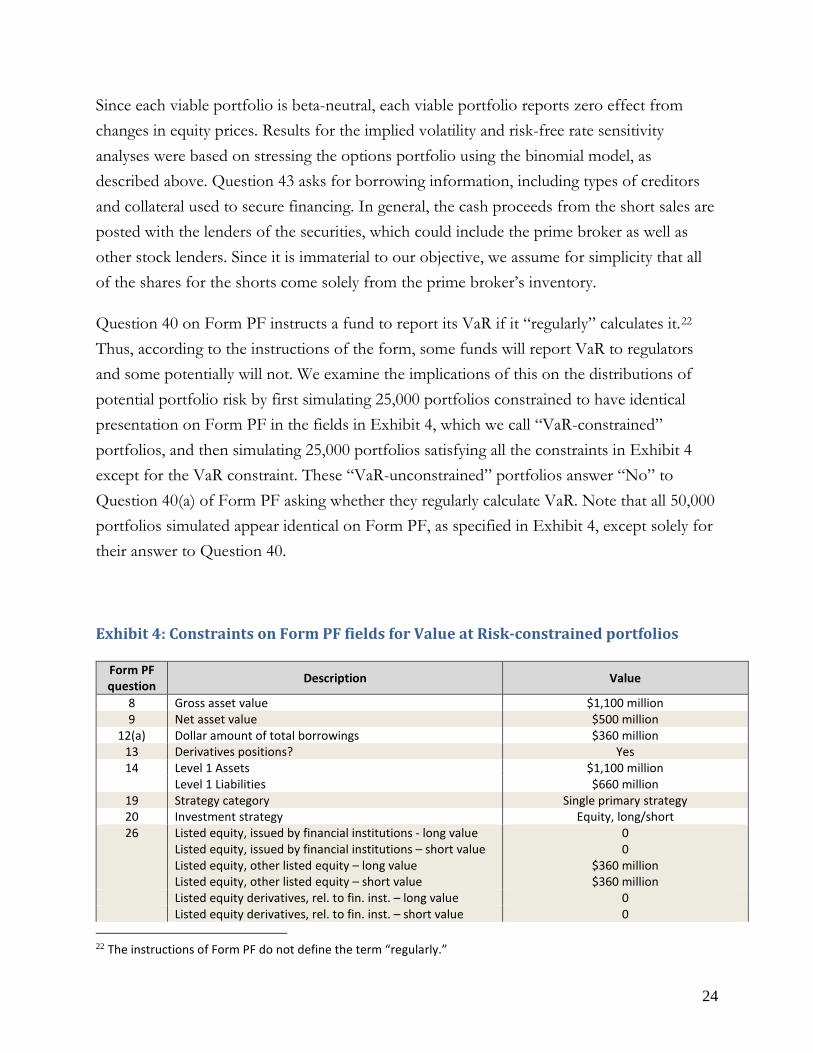
Question 40 on Form PF instructs a fund to report its VaR if it “regularly” calculates it.22 Thus, according to the instructions of the form, some funds will report VaR to regulators and some potentially will not. We examine the implications of this on the distributions of potential portfolio risk by first simulating 25,000 portfolios constrained to have identical presentation on Form PF in the fields in Exhibit 4, which we call “VaR-constrained” portfolios, and then simulating 25,000 portfolios satisfying all the constraints in Exhibit 4 except for the VaR constraint. These “VaR-unconstrained” portfolios answer “No” to Question 40(a) of Form PF asking whether they regularly calculate VaR. Note that all 50,000 portfolios simulated appear identical on Form PF, as specified in Exhibit 4, except solely for their answer to Question 40.

Exhibit 4: Constraints on Form PF fields for Value at Risk-constrained portfolios

Form PF question Description Value

8 Gross asset value $1,100 million 9 Net asset value $500 million

12(a) Dollar amount of total borrowings $360 million 13 Derivatives positions? Yes 14 Level 1 Assets $1,100 million

Level 1 Liabilities $660 million 19 Strategy category Single primary strategy 20 Investment strategy Equity, long/short 26 Listed equity, issued by financial institutions - long value

Listed equity, issued by financial institutions – short value Listed equity, other listed equity – long value Listed equity, other listed equity – short value

0 0

$360 million $360 million

Listed equity derivatives, rel. to fin. inst. – long value 0 Listed equity derivatives, rel. to fin. inst. – short value 0

22 The instructions of Form PF do not define the term “regularly.”

25

Listed equity derivatives, other – long value 0 Listed equity derivatives, other – short value $300 million

32 Liquidity – 1 day or less 100 34 Total number of open positions 65 35 Positions >5% net asset value (NAV) N.A. 40 Value at risk (VaR) 0.995 ≤ 1-day, 5%, parametric VaR < 1.005 41 Other risk metrics ES, worst day, vol, skewness 42 Equity prices increase 5% 0%

Equity prices decrease 5% 0% Equity prices increase 20% 0% Equity prices decrease 20% 0% Risk-free interest rates increase 25 basis points (bps) 0% Risk-free interest rates decrease 25 bps 0% Risk-free interest rates increase 75 bps 0% Risk-free interest rates decrease 75 bps 0% Option-implied volatilities increase 4% -2% Option-implied volatilities decrease 4% 2% Option-implied volatilities increase 10% -4% Option-implied volatilities decrease 10% 4%

43(b)(i)(A) Cash collateral posted with prime broker $80 million 43(b)(i)(B) Securities collateral posted with prime broker $360 million

44 Aggregate derivatives $300 million Source: Authors’ analysis

For the VaR-constrained portfolios, we require the daily, 5 percent parametric VaR to fall within a very narrow range around the estimated value for the benchmark portfolios. Specifically, we constrain the 1-day, 5 percent parametric VaR to be equal for all 25,000 portfolios when rounded to two decimal places of a percentage point. We call portfolios with such a constraint “VaR-constrained” portfolios. The creation of the 25,000 VaR-constrained portfolios is accomplished as follows. We first generate 6,000,000 portfolios using the portfolio formation methodology detailed above. We then sort the portfolios according to their daily 5 percent parametric VaR and randomly select 25,000 portfolios from the subset of portfolios with a daily, 5 percent parametric VaR equal to 1.00 percent.

Computing the risk and performance measures associated to a portfolio requires the portfolio’s historical returns series. This is straightforward for the equities in the portfolio, since we have each equity’s complete historical daily returns series for the period between January 2009 and December 2013. The returns series for an option position, however, has to be estimated from the returns series on its underlying. To accomplish this, we use the Greeks, specifically delta, gamma, and theta. Recall that an option’s delta is the rate of change of its premium with respect to its underlying, gamma is the rate of change of the delta with respect to its underlying, and theta is the rate of change of the premium of the

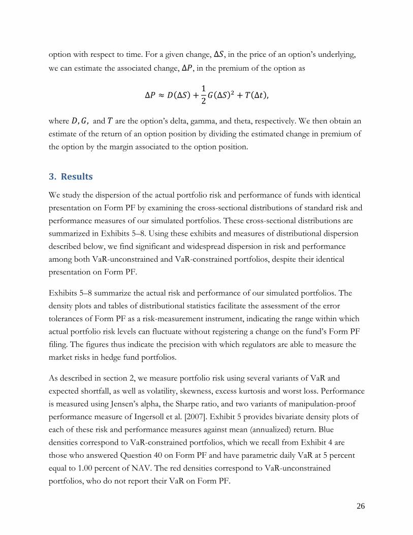
26

option with respect to time. For a given change, Δ𝑆𝑆, in the price of an option’s underlying,

we can estimate the associated change, Δ𝑃𝑃, in the premium of the option as

Δ𝑃𝑃 ≈ 𝐷𝐷(Δ𝑆𝑆) +12𝐺𝐺(Δ𝑆𝑆)2 + 𝑇𝑇(Δ𝑡𝑡),

where 𝐷𝐷,𝐺𝐺, and 𝑇𝑇 are the option’s delta, gamma, and theta, respectively. We then obtain an estimate of the return of an option position by dividing the estimated change in premium of the option by the margin associated to the option position.

3. Results

We study the dispersion of the actual portfolio risk and performance of funds with identical presentation on Form PF by examining the cross-sectional distributions of standard risk and performance measures of our simulated portfolios. These cross-sectional distributions are summarized in Exhibits 5–8. Using these exhibits and measures of distributional dispersion described below, we find significant and widespread dispersion in risk and performance among both VaR-unconstrained and VaR-constrained portfolios, despite their identical presentation on Form PF.

Exhibits 5–8 summarize the actual risk and performance of our simulated portfolios. The density plots and tables of distributional statistics facilitate the assessment of the error tolerances of Form PF as a risk-measurement instrument, indicating the range within which actual portfolio risk levels can fluctuate without registering a change on the fund’s Form PF filing. The figures thus indicate the precision with which regulators are able to measure the market risks in hedge fund portfolios.

As described in section 2, we measure portfolio risk using several variants of VaR and expected shortfall, as well as volatility, skewness, excess kurtosis and worst loss. Performance is measured using Jensen’s alpha, the Sharpe ratio, and two variants of manipulation-proof performance measure of Ingersoll et al. [2007]. Exhibit 5 provides bivariate density plots of each of these risk and performance measures against mean (annualized) return. Blue densities correspond to VaR-constrained portfolios, which we recall from Exhibit 4 are those who answered Question 40 on Form PF and have parametric daily VaR at 5 percent equal to 1.00 percent of NAV. The red densities correspond to VaR-unconstrained portfolios, who do not report their VaR on Form PF.

27

Consider the risk and performance measures depicted in Exhibit 5. We observe that the blue densities appear to be contained in the red densities, indicating that there is greater dispersion in the risk and performance measures of the VaR-unconstrained portfolios than in the VaR-constrained portfolios. In addition, focusing only on the blue densities for the VaR-constrained portfolios, we observe significant dispersion in most of the distributions, though each of these portfolios is constrained to have identical 5 percent daily VaR. Thus the plots in Exhibit 5 provide initial evidence of significant and widespread dispersion in the risk and performance measures of our simulated portfolios.

While Exhibit 5 graphically illustrates the cross-sectional distributions of the risk and performance measures of our simulated portfolios, Exhibits 6 and 7 summarize these distributions quantitatively by reporting distributional statistics for the risk and performance measures of VaR-constrained and VaR-unconstrained portfolios, respectively. In addition, we also report three tolerance ratios in Exhibits 6 and 7 to help assess the risk measurement precision of Form PF. For a given distribution, the first tolerance ratio, TR1, is defined as the ratio of the maximal value to the median value; the second tolerance ratio, TR2, is defined as the ratio of the difference between the maximum and minimum values to the median value; and the third tolerance ratio, TR3, is defined as the ratio of the interquartile range to the median value. If the risk measurement tolerances in the form were small, then we would generally expect that relevant distributions would have a small standard deviation, and tolerance ratios defined above would have values close to one, zero, and zero, respectively.

Exhibits 6 and 7, however, clearly demonstrate that dispersion in actual risk levels of portfolios is significant and widespread, even for VaR-constrained portfolios, all of which have the same daily, 5 percent parametric VaR out to one-hundredth of a percentage point of net asset value. Consider, for instance, the 12 tail risk measure variants, VaR and expected shortfall (ES), in Exhibit 6. Averaging the TR1 statistic across these 12 measures reveals that the maximum portfolio risk is on average 42 percent higher than the median risk. In addition, the maximum 1 percent, 5-trading day VaR and ES measures are 87 percent and 96 percent higher than their associated median values. The TR2 and TR3 statistics support the results of TR1. TR2, which measures the range normalized by the median, averages 0.68, with a high of 1.40. TR3, which measures the normalized interquartile range, is much smaller at 0.10, so that the interquartile range is only 10 percent of the median measure. This

28

suggests that the distributions of the risk measures are tight around their medians but have large outliers and fat tails.

The error tolerances in the VaR-unconstrained case are much higher, as is evident in the red densities in the bivariate plots of Exhibit 5. Considering the distributional statistics for the VaR-unconstrained case in Exhibit 7, we see that the TR1 statistics for the 12 variants of VaR and ES are all much higher than they are in the VaR-constrained case, with a low of 4.31, a high of 8.32, and an average of 6.35. In other words, the maximum risk conveyed by one of these risk measures for the options portfolio averages 535 percent higher than the median risk. This value is more than ten times the corresponding value, 42 percent, in the VaR-constrained case. Similarly, the TR2 and TR3 measures reveal that these portfolios also show considerable range. The TR2 measure, which is the range of the series normalized by the median, was on average 5.79, while the TR3 measure, which is the interquartile range normalized by the median, averaged 0.27.

Like the risk measures, the performance measures, i.e. Jensen’s alpha, the Sharpe ratio, and the manipulation-proof performance measures, 𝛩𝛩(0) and 𝛩𝛩(4), also show significant range. Average performance is generally better in the VaR-constrained case, with about half as much dispersion as measured by standard deviation across performance measures as the VaR-unconstrained case. Across all performance measures, the worst-performing fund in the VaR-unconstrained case has significantly worse performance than in the VaR-constrained case. The TR1 statistic shows less difference than in the risk measures case. Here the average TR1 statistics for the VaR-constrained and VaR-unconstrained cases are similar, 2.20 and 2.35, respectively. However, the TR2 and TR3 statistics show considerable differences. The average TR2 statistic for the VaR-constrained case is 2.58 while that for the VaR-unconstrained case is 6.96, nearly 3 times greater. Similarly, the average TR3 statistic among the performance measures for the VaR-constrained case is 0.41 while it is 0.63 in the VaR-unconstrained case. These results suggest that the range of performance is significantly greater on a normalized basis in the VaR-unconstrained case relative to the VaR-constrained case.

We also consider the effect of including options in a portfolio by studying the returns of the simulated funds as if they did not invest in options. That is, we consider the returns on the equities sub-portfolios of the funds. A priori, it is unclear whether the addition of options in a fund’s portfolio leads to higher or lower measurement tolerances on Form PF. Options

29

used in the pursuit of a speculative strategy could increase portfolio risk, while options used for hedging could reduce portfolio risk. In addition, the set of Form PF fields completed by a fund with a portfolio in cash equities and equity options is a superset of those completed by an equities-only fund, complicating the conclusions one can initially draw. Descriptive statistics for the equities-only sub-portfolios of our funds appear on the right-hand side of Exhibits 6 and 7, and bivariate plots of the risk and performance measures of equities-only sub-portfolios are in Exhibit 8. Considering the VaR-constrained case first, we see in Exhibit 6 that all three tolerance ratios are slightly lower but broadly similar in equities-only case for the VaR and ES risk measures. The tolerance ratios for the performance measures are about 1.5 to 2 times greater for the funds with options. By contrast, there are more significant differences in the tolerance ratios of the funds with options and funds without in the VaR-unconstrained case. The average TR1 statistics, for example, for the VaR and ES is 2.39 for the equities-only portfolios but 6.35 for the portfolios with options. Disparities of a similar magnitude are also found in the TR2 statistic.

Another point of comparison between the equities and options portfolios and the equities-only portfolios is the difference in correlations with the mean annualized return. This is clear in the bivariate plots, Exhibits 5 and 8. In the VaR-unconstrained case in Exhibit 6, the average correlation between risk measures (VaR and ES) and mean return is negative 0.81 for portfolios with options. On the other hand, the average correlation among the risk measures and mean return for equities-only portfolios is -0.01, nearly perfectly uncorrelated. This also holds in general for the VaR-constrained case, though the effect is not as large. Recall that all of the portfolios presented in the analysis are beta-neutral. One possible explanation for the observed negative correlations in the portfolios with options is that these portfolios load on a risk factor that is not priced by the market.

4. Conclusion

We review the origins of Form PF as a mechanism for systemic risk assessment and investor protection, and consider the precision of Form PF as risk measurement tool. We extend the methodology of Flood, Monin, and Bandyopadhyay [2015] to consider the effect of basic options strategies on the risks that are measured (and unmeasured) by Form PF. Although

30

the investment strategies are quite generic, the results are revealing. Applying the method to plausible examples of quantitative hedge fund strategies over portfolios of listed equities and equity options reveals significant “wiggle room” in Form PF as a risk-measurement instrument. A natural way to tighten these tolerances would be to re-stratify the characteristics that Form PF uses to represent complex portfolios, or to capture additional characteristics on the form to constrain the range of possible risk profiles more tightly. In particular, reporting of VaR under Question 40 of Form PF is currently required only if the fund regularly calculates VaR, creating the potential for funds to not report their VaRs to regulators. This question might be made mandatory, and the set of acceptable VaR methodologies specified in detail. More ambitiously, Form PF might be revamped to require position-level details of portfolio holdings, similar to the SEC’s Form 13F. Aside from the application to Form PF, the methodology of constrained risk maximization developed in Flood, Monin and Bandyopadhyay [2015] and extended herein provides a useful tool to help guide the choice of measurement dimensions.

31

References

Acharya, V.; Cooley, T.; Richardson, M. and Walter, I. (2010), “Manufacturing Tail Risk: A Perspective on the Financial Crisis of 2007–2009,” Foundations and Trends in Finance, 4(4), 247-325.

Agarwal, V.; Daniel, N. and Naik, N. (2011) “Do hedge funds manage their reported

returns?” Review of Financial Studies, 24(10), October, 3281-3320. Agarwal, V.; Gay, G. D. and Ling, L. (2014), “Window Dressing in Mutual Funds,” Review of

Financial Studies, 27(11), November, 3133–3170. Agarwal, V. and Naik, N. Y. (2004), “Risks and Portfolio Decisions Involving Hedge

Funds,” Review of Financial Studies, 17(1), January, 63–98. Aguiar, A.; Bookstaber, R. and Wipf, T. (2014), “A Map of Funding Durability and Risk,”

OFR Working Paper 14-03, May. http://financialresearch.gov/working-papers. Amin, G. S. and Kat, H. M. (2003), “Welcome to the dark side: hedge fund attrition and

survivorship bias over the period 1994–2001,” Journal of Alternative Investments, 6(1), 57–73.

Autore, D. M.; Billingsley, R. S. and Kovacs, T. (2011), “The 2008 short sale ban: Liquidity,

dispersion of opinion, and the cross-section of returns of US financial stocks,” Journal of Banking and Finance, 35(9), September, 2252–2266.

Ben-David, I.; Franzoni, F. and Moussawi, R. (2012), “Hedge Fund Stock Trading in the

Financial Crisis of 2007–2009,” Review of Financial Studies, 25(1), January, 1–54. Bernanke, B. S. (2006), “Hedge Funds and Systemic Risk,” Federal Reserve, Speech at the

Federal Reserve Bank of Atlanta’s 2006 Financial Markets Conference, Sea Island, Georgia, May 16, 2006. http://www.federalreserve.gov/newsevents/speech/Bernanke20060516a.htm

Billio, M.; Getmansky, M.; Lo, A. W. and Pelizzon, L. (2012), “Econometric measures of

connectedness and systemic risk in the finance and insurance sectors,” Journal of Financial Economics, 104(3), 535–559.

Bisias, D.; Flood, M.; Lo, A. and Valavanis, S. (2012), “A Survey of Systemic Risk Analytics,”

Annual Review of Financial Economics, 4, 255-296. Boehmer, E.; Jones, C. M. and Zhang, X. (2013), “Shackling Short Sellers: The 2008

Shorting Ban,” Review of Financial Studies, 26(6), June, 1363–1400.

32

Bollen, N. and Pool, V. (2009) “Do hedge fund managers misreport returns? Evidence from the pooled distribution,” Journal of Finance, 64(5), October, 2257-2288.

Boyson, N. M., Stahel, C. W. and Stulz, R. M. (2010), “Hedge Fund Contagion and Liquidity

Shocks,” Journal of Finance, 65(5), October, 1789–1816. Carhart, M. M. (1997), “On persistence in mutual fund performance,” Journal of Finance,

52(1), 57–82. Chan, N.; Getmansky, M.; Haas, S. M. and Lo, A. W. (2006), “Do Hedge Funds Increase

Systemic Risk?” Federal Reserve Bank of Atlanta Economic Review, Fourth Quarter, 49–80. Commodity Futures Trading Commission; Securities and Exchange Commission (2011),

“Reporting by Investment Advisers to Private Funds and Certain Commodity Pool Operators and Commodity Trading Advisers on Form PF: Final Rule,” Federal Register 76 (221), 71128–71239.

Daníelsson, J. and Zigrand, J.P. (2007), “Regulating hedge funds,” Banque de France Financial

Stability Review, 29–36. Dixon, L.; Clancy, N. and Kumar, K. B. (2012), “Hedge Funds and Systemic Risk,” technical

report, RAND Corporation. http://www.rand.org/content/dam/rand/pubs/monographs/2012/RAND_MG1236.pdf

Dudley, E. and Nimalendran, M. (2011), “Margins and Hedge Fund Contagion,” Journal of

Financial and Quantitative Analysis, 46(5), October, 1227-1257. Fama, E. F. and French, K. R. (1993), “Common risk factors in the returns on stocks and

bonds,” Journal of Financial Economics, 33(1), 3–56. ________ (1992), “The cross-section of expected stock returns,” Journal of Finance, 47(2),

427–465. Financial Crisis Inquiry Commission (FCIC) (2011), The Financial Crisis Inquiry Report: Final

Report of the National Commission on the Causes of the Financial and Economic Crisis in the United States, U.S. Government Printing Office.

Financial Stability Oversight Council (2014), Annual Report 2014, FSOC.

http://www.treasury.gov/initiatives/fsoc/studies-reports/Pages/2014-Annual-Report.aspx

Flood, M., Monin, P., and Bandyopadhyay, M. (2015), “Gauging Form PF: Data Tolerances

33

in Regulatory Reporting on Hedge Fund Risk Exposures,” OFR Working Paper 15-13, July. http://financialresearch.gov/working-papers.

Foster, D. P. and Young, H. P. (2010), “Gaming performance fees by portfolio managers,”

Quarterly Journal of Economics, 125(4), 1435–1458. French, K. (2014), “Current Research Returns,” Internet site, Dartmouth University, 2014.

http://mba.tuck.dartmouth.edu/pages/faculty/ken.french/data_library.html Garbaravicius, T. and Dierick, F. (2005), “Hedge Funds and their Implications for Financial

Stability,” ECB Occasional Paper 34, European Central Bank. http://ssrn.com/abstract=752094

Getmansky, M.; Lo, A. W. and Makarov, I. (2004), “An econometric model of serial

correlation and illiquidity in hedge fund returns,” Journal of Financial Economics, 74(3), 529–609.

Goetzmann, W. N.; Ingersoll, J. E. and Ross, S. A. (2003) “High-Water Marks and Hedge

Fund Management Contracts,” Journal of Finance, 58, 1685–1718. Greene, N. J. (2013), “SEC JOBS Act Rulemaking Creates Opportunities and Potential

Burdens for Hedge Funds Contemplating General Solicitation and Advertising,” Hedge Fund Law Report, 6(28), July.

Griffiths, M. D. and Winters, D. B. (2005), “The Turn of the Year in Money Markets: Tests

of the Risk-Shifting Window Dressing and Preferred Habitat Hypotheses,” Journal of Business 78(4), 1337–1364.

Gropp, R. (2014), “How Important Are Hedge Funds in a Crisis?” FRBSF Economic Letter

2014-11, April. Grundy, B. D.; Lim, B. and Verwijmeren, P. (2012), “Do option markets undo restrictions

on short sales? Evidence from the 2008 short-sale ban,” Journal of Financial Economics, 106, 331–348.

Healy, A. D. and Lo, A. W. (2009), “Jumping the gates: Using beta-overlay strategies to

hedge liquidity constraints,” Journal of Investment Management, 7(3), 1–20. Hodder, J. E. and Jackwerth, J. C. (2007), “Incentive Contracts and Hedge Fund

Management,” Journal of Financial and Quantitative Analysis, 42, 811–826. House Committee on Financial Services (2008), Systemic Risk in the Financial Markets, Hearing

before the Committee on Financial Services, U.S. House of Representatives, 110th Congress, July 24, 2008. http://www.gpo.gov/fdsys/pkg/CHRG-110hhrg44903/pdf/CHRG-

34

110hhrg44903.pdf ________ (2007a), “Hedge Funds and Systemic Risk in the Financial Markets,” Hearing

before the Committee on Financial Services, U.S. House of Representatives, 110th Congress, March 13, 2007. http://www.gpo.gov/fdsys/pkg/CHRG-110hhrg35405/pdf/CHRG-110hhrg35405.pdf

________ (2007b), “Hedge Funds and Systemic Risk: Perspectives of the President's

Working Group on Financial Markets,” Hearing before the Committee on Financial Services, U.S. House of Representatives, 110th Congress, July 11, 2007. http://www.gpo.gov/fdsys/pkg/CHRG-110hhrg38388/pdf/CHRG-110hhrg38388.pdf

________ (2007c), “Systemic Risk: Examining Regulators’ Ability to Respond to Threats to

the Financial System,” Hearing before the Committee on Financial Services, U.S. House of Representatives, 110th Congress, October 2, 2007. http://www.gpo.gov/fdsys/pkg/CHRG-110hhrg39903/pdf/CHRG-110hhrg39903.pdf

House Committee on Oversight and Government Reform (2008), “Hedge Funds and the

Financial Market,” Hearing before the Committee on Oversight and Government Reform, U.S. House of Representatives, 110th Congress, November 13, 2008. http://www.gpo.gov/fdsys/pkg/CHRG-110hhrg56582/pdf/CHRG-110hhrg56582.pdf

________ (2007), “After Blackstone: Should Small Investors Be Exposed To Risks Of

Hedge Funds?” Hearing before the Committee on Oversight and Government Reform, U.S. House of Representatives, 110th Congress, July 11, 2007. http://www.gpo.gov/fdsys/pkg/CHRG-110hhrg44903/pdf/CHRG-110hhrg44903.pdf

Huang, J.-Z. and Wang, Y. (2013), Hedge Funds and the Financial Crisis, in H. Kent Baker

and Greg Filbeck, ed., Alternative Investments: Instruments, Performance, Benchmarks, and Strategies, John Wiley and Sons.

Ingersoll, J.; Spiegel, M.; Goetzmann, W. and Welch, I. (2007), “Portfolio performance

manipulation and manipulation-proof performance measures,” Review of Financial Studies 20(5), 1503–1546.

Jacobs, B. and Levy, K. (1997), “The Long and Short on Long-Short,” Journal of Investing,

6(1), Spring, 73–88. Jorion, P. (2000) Value at Risk: The New Benchmark for Managing Financial Risk, McGraw-Hill. Kambhu, J.; Schuermann, T. and Stiroh, K. J. (2007), “Hedge funds, financial

intermediation, and systemic risk,” FRB of New York Staff Report (291), Federal Reserve Bank of New York. http://www.nyfedeconomists.org/research/staff_reports/sr291.pdf

35

Khandani, A. and Lo, A. W. (2011), “What Happened To The Quants In August 2007?

Evidence from Factors and Transactions Data,” Journal of Financial Markets, 14, 1–46. Lakonishok, J.; Shleifer, A.; Thaler, R. and Vishny, R. (1991), “Window Dressing by Pension

Fund Managers,” American Economic Review, 81(2), 227–31. Lan, Y.; Wang, N. and Yang, J. (2013), “The economics of hedge funds,” Journal of Financial

Economics, 110(2), 300–323. Lo, A. W. (2009), “Regulatory reform in the wake of the financial crisis of 2007-2008,”

Journal of Financial Economic Policy, 1(1), 4–43. ________ (2008), “Hedge Funds, Systemic Risk, and the Financial Crisis of 2007-2008:

Written Testimony for the House Oversight Committee Hearing on Hedge Funds,” MIT, November 13, 2008. http://ssrn.com/abstract=1301217

________ (2001), “Risk management for hedge funds: Introduction and overview,” Financial

Analysts Journal, 16–33. Lo, A. W. and Patel, P. N. (2008), “130/30: The New Long-Only,” Journal of Portfolio

Management, 34(2), 12–38. Lowenstein, R. (2000), When Genius Failed: The Rise and Fall of Long-Term Capital Management,

Random House. Mitchell, M. and Pulvino, T. (2012), “Arbitrage crashes and the speed of capital,” Journal of

Financial Economics, 104(3), June, 469–490. ________ (2001), “Characteristics of risk and return in risk arbitrage,” Journal of Finance,

56(6), December, 2135–2175. Office of Financial Research (OFR) (2015), Financial Stability Report 2015, technical report,

December. https://financialresearch.gov/financial-stability-reports/files/OFR_2015-Financial-Stability-Report_12-15-2015.pdf

Ortiz, C.; Sarto, J. L. and Vicente, L. (2012), “Portfolios in disguise? Window dressing in

bond fund holdings,” Journal of Banking and Finance, 36(2), 418–427. Parry, H. (2001), “Hedge Funds, Hot Markets and the High Net Worth Investor: A Case for

Greater Protection,” Northwestern Journal of International Law and Business 21(3), 703–722. Patton, A. J. and Ramadorai, T. (2013), “On the High-Frequency Dynamics of Hedge Fund

Risk Exposures,” Journal of Finance, 68(2), 597–635.

36

President’s Working Group on Financial Markets (2007), “Agreement among PWG and U.S.

Agency Principals on Principles and Guidelines Regarding Private Pools of Capital,” Technical report, U.S. Department of the Treasury. http://www.treasury.gov/resource-center/fin-mkts/Documents/hp272_principles.pdf

________ (1999), “Hedge Funds, Leverage, and the Lessons of Long-Term Capital

Management (LTCM),” Technical report, U.S. Department of the Treasury. http://www.treasury.gov/resource-center/fin-mkts/Documents/hedgfund.pdf

Securities and Exchange Commission (SEC) (2015), “Form PF: Frequently Asked

Questions,” technical document, accessed 16 March 2015. http://www.sec.gov/divisions/investment/pfrd/pfrdfaq.shtml.

________ (2011), “FORM PF: Reporting Form for Investment Advisers to Private Funds

and Certain Commodity Pool Operators and Commodity Trading Advisers,” reporting form SEC 2048 (OMB Number: 3235-0679). http://www.sec.gov/about/forms/formpf.pdf

________ (2010), “Investigation of the SEC’s Response to Concerns Regarding Robert

Allen Stanford’s Alleged Ponzi Scheme,” Inspector General’s report, SEC Case No. OIG-526. http://www.sec.gov/news/studies/2010/oig-526.pdf

________ (2009), “Investigation of Failure of the SEC to Uncover Bernard Madoff’s Ponzi

Scheme - Public Version,” Inspector General’s report, SEC Case No. OIG-509. http://www.sec.gov/news/studies/2009/oig-509.pdf

________ (1997), “Privately Offered Investment Companies,” Federal Register, 62(68), April

9, 17512–17529. ________ (1992), “Protecting Investors: A Half Century of Investment Company

Regulation,” SEC Division of Investment Management. http://www.sec.gov/divisions/investment/guidance/icreg50-92.pdf

Sialm, C., Sun, Z. and Zheng, L. (2013), “Home Bias and Local Contagion: Evidence from

Funds of Hedge Funds,” NBER Working Paper w19570. http://www.nber.org/papers/w19570.

Sias, R. (2007), “Causes and Seasonality of Momentum Profits,” Financial Analysts Journal,

63(2), 48–54. Sias, R. W. and Starks, L. T. (1997), “Institutions and Individuals at the Turn-of-the-Year,”

Journal of Finance, 52(4), 1543–1562.

37

Stein, R. M. (2012), “The Role of Stress Testing in Credit Risk Management,” Journal of

Investment Management, 10(4), 64-90. Stulz, R. M. (2007), “Hedge Funds: Past, Present, and Future,” Journal of Economic Perspectives,

21(2), Spring, 175–194. U.S. Congress (1996), “National Securities Markets Improvement Act of 1996,” October.

http://www.gpo.gov/fdsys/pkg/PLAW-104publ290/pdf/PLAW-104publ290.pdf. ________ (2010), “Dodd-Frank Wall Street Reform and Consumer Protection Act,” July.

http://www.gpo.gov/fdsys/pkg/PLAW-111publ203/pdf/PLAW-111publ203.pdf Wermers, R. (2012), “Matter of Style: The Causes and Consequences of Style Drift in

Institutional Portfolios,” working paper, University of Maryland. http://ssrn.com/abstract=2024259

White, M. J. (2014), “Enhancing Risk Monitoring and Regulatory Safeguards for the Asset

Management Industry,” Securities and Exchange Commission, Speech to The New York Times DealBook Opportunities for Tomorrow Conference, New York City, December 11, 2014. http://www.sec.gov/News/Speech/Detail/Speech/1370543677722#.VMLSvfldVCY

38

Exhibit 5: Plots of risk and performance measures against annualized mean return for funds with portfolios of equities and equity options

Blue = VaR-constrained, Red = VaR-unconstrained. Sources: Center for Research in Security Prices, OptionMetrics LLC, OFR analysis

39

Exhibit 6: Summary statistics for VaR-constrained portfolios

Sources: Center for Research in Security Prices, OptionMetrics LLC, OFR analysis

Mean S.dev. Min 25% 50% 75% Max TR1 TR2 TR3 Corr. MR

Mean S.dev. Min 25% 50% 75% Max TR1 TR2 TR3 Corr. MR

VaR (HS), 5%, daily 0.93 0.05 0.72 0.91 0.94 0.97 1.10 1.17 0.40 0.06 -0.14 0.93 0.03 0.80 0.90 0.93 0.95 1.08 1.16 0.30 0.05 -0.13

VaR (HS), 1%, daily 1.69 0.12 1.25 1.62 1.69 1.77 2.28 1.35 0.61 0.09 -0.08 1.58 0.09 1.23 1.51 1.58 1.64 2.14 1.35 0.58 0.08 -0.15

VaR (HS), 5%, 5-td 1.85 0.18 1.21 1.73 1.84 1.96 2.88 1.57 0.91 0.13 -0.71 1.74 0.11 1.33 1.67 1.74 1.82 2.27 1.30 0.54 0.09 -0.38

VaR (HS), 1%, 5-td 3.38 0.44 2.19 3.08 3.33 3.64 6.22 1.87 1.21 0.17 -0.43 2.95 0.28 2.03 2.75 2.93 3.12 4.57 1.56 0.87 0.13 -0.28

VaR (P), 5%, daily 1.00 0.00 1.00 1.00 1.00 1.00 1.00 1.00 0.00 0.00 -0.01 1.00 0.00 1.00 1.00 1.00 1.00 1.00 1.00 0.00 0.00 0.02

VaR (P), 1%, daily 1.45 0.01 1.40 1.45 1.45 1.46 1.50 1.03 0.07 0.01 0.94 1.46 0.01 1.44 1.46 1.46 1.47 1.48 1.01 0.03 0.01 0.71

VaR (P), 5%, 5-td 1.96 0.13 1.50 1.87 1.96 2.05 2.58 1.32 0.55 0.09 -0.72 1.89 0.09 1.54 1.83 1.89 1.95 2.26 1.20 0.38 0.06 -0.30

VaR (P), 1%, 5-td 2.97 0.14 2.42 2.88 2.97 3.07 3.59 1.21 0.39 0.06 -0.49 2.91 0.13 2.44 2.82 2.91 2.99 3.43 1.18 0.34 0.06 -0.16

ES, 5%, daily 1.34 0.06 1.02 1.31 1.34 1.38 1.60 1.19 0.43 0.05 -0.14 1.28 0.04 1.09 1.25 1.28 1.31 1.49 1.16 0.31 0.05 -0.21

ES, 1%, daily 2.13 0.16 1.54 2.02 2.13 2.23 2.91 1.37 0.64 0.10 -0.12 1.94 0.12 1.49 1.85 1.93 2.02 2.49 1.29 0.52 0.09 -0.14

ES, 5%, 5-td 2.68 0.26 1.83 2.49 2.66 2.84 4.08 1.53 0.85 0.13 -0.60 2.40 0.17 1.78 2.28 2.40 2.52 3.30 1.38 0.63 0.10 -0.36

ES, 1%, 5-td 4.31 0.70 2.36 3.81 4.20 4.70 8.25 1.96 1.40 0.21 -0.28 3.63 0.45 2.30 3.31 3.58 3.90 6.39 1.78 1.14 0.16 -0.24

Vol. (annualized) 10.58 0.28 9.38 10.40 10.60 10.77 11.59 1.09 0.21 0.03 0.99 10.75 0.10 10.41 10.69 10.75 10.82 11.14 1.04 0.07 0.01 0.96

Skewness -0.22 0.59 -6.76 -0.35 -0.10 0.08 1.73 -17.30 -84.90 -4.30 0.25 0.24 0.18 -0.47 0.12 0.23 0.36 1.37 5.96 8.00 1.04 0.26

Ex. Kurtosis 5.17 7.21 0.62 2.35 3.19 4.85 134.23 42.08 41.88 0.78 -0.06 2.33 0.86 0.38 1.73 2.18 2.76 11.08 5.08 4.91 0.47 0.07

Worst loss (1-td) 3.98 1.55 1.93 2.97 3.44 4.44 12.99 3.78 3.22 0.43 -0.13 2.88 0.45 1.76 2.56 2.82 3.13 5.71 2.02 1.40 0.20 -0.05

Jensen's alpha 25.14 7.59 -8.65 20.35 25.74 30.44 53.69 2.09 2.42 0.39 0.94 29.89 3.42 17.41 27.56 29.87 32.23 42.78 1.43 0.85 0.16 0.64

Sharpe ratio 2.38 0.79 -0.71 1.87 2.40 2.91 5.83 2.43 2.73 0.43 0.85 2.76 0.44 1.26 2.45 2.73 3.04 5.17 1.89 1.43 0.22 0.41

Theta (rho=0) 0.25 0.07 -0.09 0.20 0.25 0.30 0.53 2.12 2.48 0.40 0.94 0.30 0.03 0.17 0.27 0.30 0.32 0.42 1.40 0.83 0.17 0.64

Theta (rho=4) 0.23 0.08 -0.12 0.18 0.23 0.28 0.50 2.17 2.70 0.43 0.93 0.27 0.03 0.14 0.25 0.27 0.30 0.41 1.52 1.00 0.19 0.63

Mean return (annualized) 24.14 7.20 -7.09 19.63 24.81 29.18 50.59 2.04 2.32 0.38 1.00 28.73 2.43 20.17 27.07 28.69 30.34 38.48 1.34 0.64 0.11 1.00

EQUITIES AND EQUITY OPTIONS EQUITIES ONLY

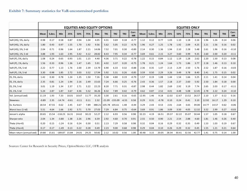
40

Exhibit 7: Summary statistics for VaR-unconstrained portfolios

Sources: Center for Research in Security Prices, OptionMetrics LLC, OFR analysis

Mean S.dev. Min 25% 50% 75% Max TR1 TR2 TR3 Corr. MR

Mean S.dev. Min 25% 50% 75% Max TR1 TR2 TR3 Corr. MR

VaR (HS), 5%, daily 0.98 0.17 0.58 0.87 0.94 1.04 4.05 4.31 3.69 0.18 -0.77 1.12 0.12 0.77 1.03 1.10 1.18 2.16 1.96 1.26 0.14 0.06

VaR (HS), 1%, daily 1.80 0.43 0.97 1.55 1.70 1.92 9.56 5.62 5.05 0.22 -0.76 1.96 0.27 1.25 1.78 1.92 2.09 4.25 2.21 1.56 0.16 0.02

VaR (HS), 5%, 5-td 2.04 0.71 0.96 1.64 1.87 2.21 14.06 7.52 7.01 0.30 -0.89 2.14 0.30 1.36 1.94 2.10 2.28 5.48 2.61 1.96 0.16 -0.10

VaR (HS), 1%, 5-td 3.88 1.93 1.63 2.95 3.42 4.12 28.82 8.43 7.95 0.34 -0.77 3.69 0.61 2.15 3.27 3.60 3.99 9.35 2.60 2.00 0.20 -0.11

VaR (P), 5%, daily 1.08 0.24 0.65 0.93 1.01 1.15 4.40 4.36 3.71 0.22 -0.78 1.22 0.15 0.84 1.12 1.19 1.28 2.62 2.20 1.50 0.13 0.08

VaR (P), 1%, daily 1.56 0.33 0.96 1.36 1.47 1.65 5.91 4.02 3.37 0.20 -0.75 1.78 0.21 1.24 1.64 1.73 1.86 3.77 2.18 1.46 0.13 0.10

VaR (P), 5%, 5-td 2.22 0.77 1.13 1.76 2.00 2.39 13.79 6.90 6.33 0.32 -0.88 2.36 0.35 1.47 2.13 2.29 2.50 5.76 2.52 1.87 0.16 -0.03

VaR (P), 1%, 5-td 3.30 0.98 1.85 2.72 3.03 3.52 17.94 5.92 5.31 0.26 -0.85 3.59 0.50 2.29 3.26 3.49 3.78 8.40 2.41 1.75 0.15 0.02

ES, 5%, daily 1.42 0.30 0.78 1.24 1.35 1.50 7.26 5.38 4.80 0.19 -0.79 1.57 0.19 1.08 1.44 1.54 1.66 3.25 2.11 1.41 0.14 0.04

ES, 1%, daily 2.35 0.81 1.24 1.94 2.16 2.49 15.63 7.24 6.66 0.25 -0.76 2.43 0.36 1.57 2.18 2.37 2.60 5.92 2.50 1.84 0.18 0.00

ES, 5%, 5-td 3.01 1.19 1.34 2.37 2.71 3.22 22.23 8.20 7.71 0.31 -0.87 2.98 0.44 1.82 2.69 2.92 3.19 7.74 2.65 2.03 0.17 -0.11

ES, 1%, 5-td 5.24 2.87 1.87 3.67 4.36 5.52 36.26 8.32 7.89 0.42 -0.79 4.62 0.87 2.52 4.01 4.48 5.08 12.45 2.78 2.22 0.24 -0.10

Vol. (annualized) 11.19 1.93 7.33 10.01 10.67 11.77 35.20 3.30 2.61 0.16 -0.65 12.95 1.46 9.18 12.02 12.67 13.52 26.57 2.10 1.37 0.12 0.16

Skewness -0.89 2.35 -14.74 -0.61 -0.11 0.11 2.32 -21.09 -155.09 -6.55 0.58 0.29 0.31 -0.78 0.10 0.24 0.41 3.10 12.92 16.17 1.29 0.10

Ex. Kurtosis 18.54 47.55 0.62 2.45 3.67 7.89 388.21 105.78 105.61 1.48 -0.44 3.29 2.43 0.53 2.01 2.64 3.65 39.00 14.77 14.57 0.62 -0.06

Worst loss (1-td) 5.51 4.64 1.66 2.92 3.71 5.70 27.03 7.29 6.84 0.75 -0.64 3.69 0.91 1.86 3.09 3.50 4.05 12.32 3.52 2.99 0.27 -0.03

Jensen's alpha 20.65 15.54 -118.23 16.31 24.62 30.22 52.27 2.12 6.93 0.56 0.98 32.23 4.19 16.51 29.37 32.22 35.07 50.44 1.57 1.05 0.18 0.67

Sharpe ratio 2.04 1.34 -3.80 1.38 2.26 2.96 6.59 2.92 4.60 0.70 0.91 2.55 0.50 0.90 2.21 2.54 2.88 4.60 1.81 1.46 0.26 0.40

Theta (rho=0) 0.20 0.15 -1.24 0.16 0.24 0.30 0.51 2.13 7.29 0.58 0.98 0.32 0.04 0.16 0.29 0.32 0.35 0.49 1.53 1.03 0.19 0.67

Theta (rho=4) 0.17 0.17 -1.49 0.13 0.22 0.28 0.49 2.23 9.00 0.68 0.98 0.29 0.04 0.10 0.26 0.29 0.32 0.45 1.55 1.21 0.21 0.64

Mean return (annualized) 19.80 15.61 -189.87 15.84 24.01 29.25 50.82 2.12 10.02 0.56 1.00 30.48 3.15 20.05 28.34 30.41 32.56 42.77 1.41 0.75 0.14 1.00

EQUITIES AND EQUITY OPTIONS EQUITIES ONLY

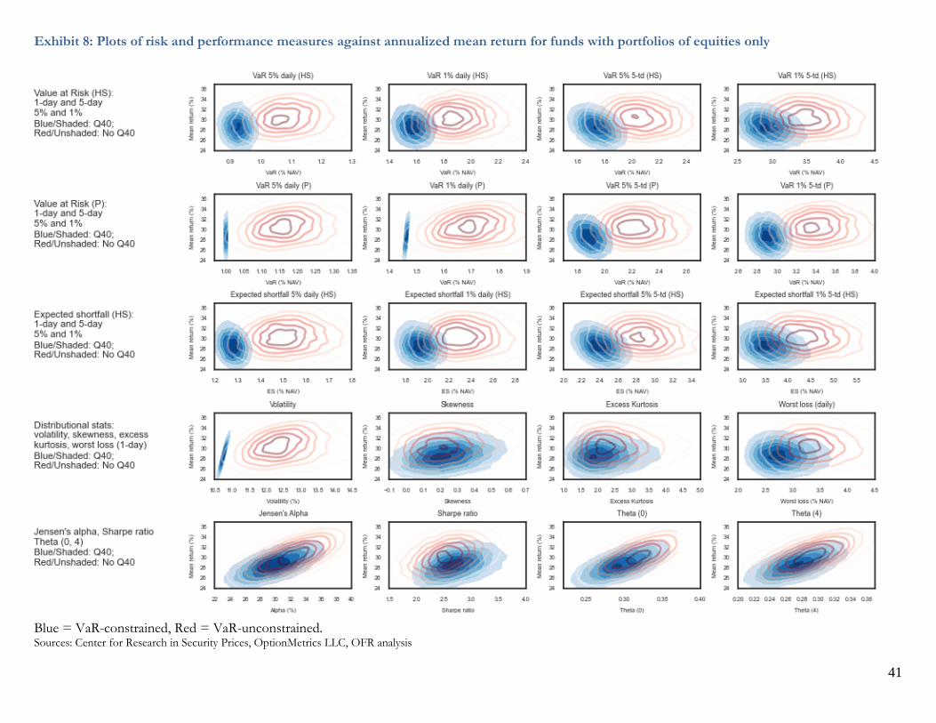
41

Exhibit 8: Plots of risk and performance measures against annualized mean return for funds with portfolios of equities only

Blue = VaR-constrained, Red = VaR-unconstrained. Sources: Center for Research in Security Prices, OptionMetrics LLC, OFR analysis