formal description for an object-oriented role-based
TRANSCRIPT

Vol. 2, No. 2 Computer and Information Science
68
Formal Description for an Object-Oriented
Role-based Access Control Model Chungen Xu
Department of Applied Mathematics, Nanjing University of Science & Technology Jiangsu 210094, China
Tel: 86-25-8431-5877 E-mail: [email protected]
Sheng Gong Library, Nanjing University of Science & Technology
Jiangsu 210094, China
Abstract Role-based access control(RBAC) is a promising technology for managing and enforcing security in large-scale enterprise-wide system, and we were motivated by the need to manage and enforce the strong access control technology of RBAC in large-scale Web environments. Majority of traditional access control models were passive data-protections, which were not suitable for large and complex multi-user interactive applications. In this paper, we develop a general model to control users’ behaviors based on their roles actively, and proposes a framework of well-defined Formal Description for developers to build application-level access control based on users’ roles. It ensure that each role is configured with consistent privileges, each actor is authorized to proper roles and then each actor can activate and play his authorized roles without interest conflicts. These formal specifications are consistent and inferable, complete and simplified, abundant and scalable for diversified multi-user applications. Keywords: Object-Oriented, Formal description, Role, Access control 1. Introduction Nowadays multi-user applications tend to be large and complex. The functions and structures of large applications are complicated and distributed. And thousands of users perform their diversified duties. All these increase complexity of privilege management, and lead to low control efficiency of users’ interaction. Role-Based Access Control(RBAC)(Sandhu, 1996,p.38-47)is a successful technology that will be a central component of emerging enterprise security infrastructures. Moreover, dynamic management and collaborative control are difficult to come into effect in the large-scale Web environment. So the quality of software on the web must get most improvement. Majority of well-known access control models are passive ones, such as typical subject-object model, that are often implemented by Access Control List (ACL) or access control matrices, and Lattice-based Access Control (LBAC) and many others. These models focus on data-protections at the back-end of applications, and they do not distinguish permission assignment from activation, and further, are not capable of representing or considering any levels of context when processing an operation on an object. Recently, some works address active security models. Such as Task-based Authorization Controls model(Gavrila,1998,p.81-90), and workflow authorization model(Yan, 2000,p.1064-1071) These models consider somewhat context associated with tasks and workflow. Our focus in this paper is on a general model to control users’ behaviors actively based on their roles. Object Technology is used in the model, which is built in Unified Modeling Language (UML)( UML Summary Version2.0.,2006). Users’ behaviors are abstracted as request services and get results. Thus, user services are protected via a special interface, regardless of complexity of internal implements of these services to simplify management. Role is used to organize behavior specifications of numerous users to reduce the burden of privilege management. Role-Playing is introduced to denote activated role in particular context, and it is modeled as an active class. Every object of Role-Playing runs in particular context, which interact with a user and controls the user’s behaviors actively. Users work in collaborative environment. Users use their rights, also perform their obligations. The states, behaviors and lifetime of Role-Playing objects can be monitored or audited to support dynamic management and business

Computer and Information Science May, 2009
69
activities control. In this paper, we proposes a framework of well-defined Formal Description for developers to build application-level access control based on users’ roles. It ensure that each role is configured with consistent privileges, each actor is authorized to proper roles and then each actor can activate and play his authorized roles without interest conflicts. 2. Model elements and constraint semantics Figure 1 represents the model. Service is an interface, in which user-services are collected, and they are associated with Roles by PA; Actors are made members of proper roles by SA objects; At runtime actors activate some of their authorized roles with Role-Playing objects created and acquire authorized services. As there are complex structural and semantic relations between protected objects in a large application, the model builds a Service interface, thereby interface structure, dynamic privilege and privilege implication specifications are specified. Notice that, any interface cannot be instantiated any object, therefor an element of Service is a service item rather than an object of it. Privilege_Authorization (PA) class is an association class between Role and Service. An instance of it is a tuple (r, s) denoted by pa(r, s), which means role r has permission to a service item s under a context condition specified in its attribute: context_cond. Usually a permission of an operation implies another one, The implication relation is denoted by 21 ss cf⎯→⎯ , where cf is a function converting the context condition of s1 to that of s2. A large application may contain numerous and complex associated roles. The model supports role’s cardinality constraint, Role Inheritance (RI), one kind of hierarchy structure, and Separation of Duties (SD) to signify interest conflict relations. Status_Authorization (SA) is an association class between Actor and Role. An instance of it is a tuple (a, r) denoted by sa(a, r), which means the actor a has been authorized to role r. An instance of Separation of Duties (SD) is a tuple(role1, role2) representing conflict of interest between them. There are two subtypes of SD: Static Separation of Duties (SSD) and Dynamic Separation of Duties (DSD). At runtime actors activate and play their authorized roles to perform their duties according with privilege specifications. To signify the activated roles, the model introduces Role-Playing. A role-playing is a performance of one role r activated by an actor a in particular context, which is an active object denoted by rpa, r. An instance of Role-Playing(RP) class is a role-playing object running in particular context denoted by rpa,r.context. A role r is activated, if and only if there exists at least one rpx, r. 3. Formal specifications of constraint As the model uses many associations representing relations of objects, a set of specifications for association is set as global constraints firstly. 3.1 Specifications for a role’s privileges to services F1. A service item in Service is either an operation or an interface:
)( InterfacesOperationsServicess ∈∨∈↔∈∀
F2. Each operation is declared in particular interface: iopInterfaceiOperationop <,∈∃→∈∀
Where iop < means that operation op is declared in interface i.
F3. Generalization between interfaces is built in strict partial orders: irreflexive, anti-symmetric and transitive. F4. A PA object is a permission of a role to a service with context condition:
))()_).,((),((, srcondcontextsrpaCCPAsrpaServicesRoler cc⎯→⎯→↔∈∃∈∈∀
Where CC(pa(r, s).context_cond) means that current context satisfy the condition: pa(r, s).context_cond. sr cc⎯→⎯ means that role r has permission for service s under current context cc. F5. If a role has authorization to an operation, then the interface in which the operation declared is authorized:
)_).,(_).,(',),('),((,,
condcontextsrpacondcontextirpaPAirpaisPAsrpaInterfaceiOperationsRoler
=∈∃→∧∈∃∈∀∈∀∈∀ <
F6. If a role has authorization to an interface, then the super-interface of it is authorized:
)_).,(_).',(',)',('),'(),((',,
condcontextsrpacondcontextsrpaPAsrpationGeneralizassgPAsrpaInterfacessRoler
=∈∃→∈∃∧∈∃∈∀∈∀

Vol. 2, No. 2 Computer and Information Science
70
F7. If an operation implies another one, and a role has authorization to the operation, then the implied one is authorized with context condition conversion:
))_).,((_).,(,),(),()((,,
112222
112121
condcontextsrpacfcondcontextsrpaPAsrpaPAsrpassOperationssRoler cf
=∈∃→∈∃∧⎯→⎯∈∀∈∀
Where 21 ss cf⎯→⎯ denote operation s1 imply s2 with context condition conversion by cf. cf(pa1(r,s1).context_cond) converts
context condition of pa1 to that of pa2. Below inference is derived from F4 and predicate logic: For role r and service s, if more than one pa(r, s) objects are derived from F5, F6 or F7 or defined directly, then finally only one pa(r, s) exists as a substitute with their context conditions union:
)_).,(_).,(_).,(,),(),(),,((,
21
21
condcontextsrpacondcontextsrpacondcontextsrpaPAsrpaPAsrpasrpaServicesRoler
∨=∈∃→∈∃∈∀∈∀
3.2 Specifications for associations F8. Each tuple value in an association class appears at most once:
''',)','('),,(), ,( ttbbaaCbatbatBAAssoCC =→=∧=∈∀∈∀
where AssoC(A,B) is a set of association classes of class A and B. F9. If a tuple exist in an association class, then its associated objects must exist in the associated classes respectively:
( ) BbAaCbatBAAssoCC ∈∃∧∈∃→∈∀∈∀ ),(,,
F10. If class A associate with B, and the minimum of multiplicity of the associate end to A is 1, and if one object b exist in B, then at least one object exists in A linking with b:
),(, 1 ).min(,),( balinkAaBbmultipACBAAssoCC ∈∃→∈∀∧=>−∈∀
Where C->A.multip is the multiplicity of C association end to A, and Link(a, b) means that object a links with b. F8 and F9 apply to PA, RI, SD, SA et al. F8 ensures the objects consistency of association classes. F9 and F10 indicate that prerequisite of associated object existence. For example in Figure 1, when a Role-Playing object rpa, r exist, then a SA object sa(a,r) must exist by F10, and then the a exist in Actor and the r exist in Role by F9. F9 and F10 ensure that the associated object cannot be removed before the associating objects are removed. 3.3 Specifications for roles’ relations and authorizations F11. The Role Inheritance (RI) relation ri(super-role, sub-role) are strict partial orders: irreflexive, anti-symmetric and transitive. F12. The Separation of Duties (SD) relation sd(r1, r2) are irreflexive, symmetric and intransitive. F13. The SD is exclusive with RI for any two roles:
)),(),(),((, 1222112121 RIrrriRIrrriSDrrsdRolerr ∈¬∃∧∈¬∃→∈∃∈∀
F14. If a role inherits another role that is in SD with a third role, then the sub-role is in SD relation with the third one: )),('),(),((,, 221121 SDrrsdSDrrsdRIrrriRolerrr ∈∃→∈∃∧∈∃∈∀
F15. The SD has Static Separation of Duties (SSD) and Dynamic Separation of Duties (DSD) as its sub-type: )),(),(),((, 21212121 DSDrrdsdSSDrrssdSDrrsdRolerr ∈∃∨∈∃↔∈∃∈∀
F16. The SSD relation is exclusive with DSD for any two roles: )),(),((, 212121 DSDrrdsdSSDrrssdRolerr ∈¬∃→∈∃∈∀
F17. If one role inherits another and an actor is authorized for the sub-role, then the actor is also authorized for its super-role:
)),(),(),((,, 12212121 SArasaSArasaRIrrriActoraRolerr ∈∃→∈∃∧∈∃∈∀∈∀
F18. If a role has a privilege to a service, then the role has the privilege override the privileges of its super-roles to the service:
))()_).,((),(),'('),'((,',
srcondcontextsrpaCCPAsrpaPAsrpaRIrrriServicesRolerr
cc⎯→⎯→→∈∃∧
∈∃∧∈∃∈∀∈∀
F19. If a role has not privileges to a service, then the role inherits the non-overridden privileges of its super-roles. (The formal inheritance algorithm will be discussed elsewhere as its complexity) F20. The number of authorized actors for any role does not exceed the authorized cardinality of the role:
)_.|),(( ycardinalitauthorizedrActoraSArasaRoler ≤∈∈∈∀

Computer and Information Science May, 2009
71
F21. An actor cannot be authorized for two roles in SSD relation:
)),(),(),((,,
2
12121
SArasaSArasaSSDrrssdRolerrActora
∈¬∃→∈∃∧∈∃∈∀∈∀
Below inferences can be derived from above specifications: If one role inherits another, the authorized cardinality of the sub-role cannot exceed that of its super-roles. There is no role inheriting two roles in SD relation. 3.4 Specifications for activated roles F22. The activated number of a role does not exceed its activated cardinality:
)_.|,( ycardinalitactivatedrActoraPlayingRolerarpRoler ≤∈−∈∈∀
F23. An actor cannot activate two roles in DSD relation:
),,),((,,
2
12121
PlayingRolerarpPlayingRolerarpDSDrrdsdRolerrActora
−∈¬∃→−∈∃∧∈∃∈∀∈∀
F24. An actor activates a role no more than once in same context: , ( , ' , , ' , . , . )a Actor r Role rp a r Role Playing rp a r Role Playing rp a r context rp a r context∀ ∈ ∀ ∈ ∃ ∈ − → ¬∃ ∈ − =
F25. If an actor activate a sub-role in a context, then its super-role is activated in the same context: 1 2 1 2 2 1 1 2, , ( ( , ) , ' , , ' , . , . )a Actor r r Role ri r r RI rp a r Role Playing rp a r Role Playing rp a r context rp a r context∀ ∈ ∀ ∈ ∃ ∈ ∧∃ ∈ − →∃ ∈ − =
4. Conclusion Formal Description specifications for application-level access control are challenging and imperative works. This paper provides a novel framework of formal specifications, in which contain formal, consistent and inferable constraints. They are more complete and simplified than traditional ones, but also they are general and scalable for a wide range of multi-user interactive computing and distributed information–processing systems. The concept of usage control (UCON)( Ferraiolo,2001,224-274.and Zhang, 2008,p.1-36.)]is an important access control system after RBAC and introduced as a unified approach to capturing a number of extensions for access control models and systems. In UCON, a control decision is determined by three aspects: authorizations, obligations and conditions. We will give the formal specification of UCON in the future. References Dewan,D. and Shen,H. (1998). Controlling access in multiuser interface, ACM Transactions on Computer-Human Interaction, Volume 5, No. 1, 34-62. Enterprise JavaBeans Developers Guide (1999). [Online] http:/ /java.sun.com /products /ejb/ devguide. (Aug., 1999) Ferraiolo, D. Sandhu, R. (2001). Proposed NIST Standard for Role-Based Access Control, ACM Trans. on Information and System Security (TISSEC), 4(3) Aug. 2001, 224-274. Gavrila,S.I. and Barkley,J.F. (1998). Formal specification for role based access control user/role and role/role relationship management. RBAC '98. Proceedings of the third ACM workshop on Role-based access control, Oct. 22-23, 1998, Fairfax, VA, 81-90. Jonathan D. M. (1998). Control principles and role hierarchies, RBAC '98. Proceedings of the third ACM workshop on Role-based access control, Oct. 22-23, 1998, Fairfax, VA, 63-69. Sandhu ,R.S., Coyne,E.J., Feinstein,H.L., and Youman,C.E. (1996). Role-Based Access Control Models. IEEE Computer, Volume 29, Number 2, 38-47. UML Summary Version2.0. (2006). UML Semantics Version2.0,UML Notation Guide. [Online] Available at: http://www-01.ibm.com/software/rational/uml/ (Aug.,2006). Yan, H., Zhang, H. and Xu, M.W. (2000). Object modeling and implementation of access control based on role, Chinese Journal of Computers, v 23, n 10, 1064-1071. Zhang, X.,Nakae, M., Covington, M. and Sandhu, R. (2008). Toward a Usage-Based Security Framework for Collaborative Computing Systems, ACM Trans. on Information and System Security. (TISSEC), Volume 11, Number 1, 1-36.

Vol. 2, No. 2 Computer and Information Science
72
RoleActor <<interface>>Service
Privilege_Authorize(PA)Status_Authorize(SA)
activeRole-Playing
Role_Relation Service_Relation
messaging
* * **
*
*
*
*
* ** *
* *
*
1
1
1
interact
performactivate verify
invoke/return*
*
Figure 1. The class diagram of the model

Computer and Information Science May, 2009
73
SDS: A Scalable Data Services System in Data Grid Xiaoning Peng
School of Information Science & Engineering, Central South University Changsha 410083, China
Department of Computer Science and Technology, Huaihua College Huaihua 418008, China
Bin Huang
Department of Computer Science and Technology, Huaihua College Huaihua 418008, China
Ping Luo
Department of Computer Science and Technology, Tsinghua University Beijing 100084, China
Abstract It is very complex and of low efficiency for grid users to access heterogeneous diverse data resources distributed over the whole wide area network. Data Grid has denoted a network of storage resources, from archival systems, to caches, to databases, that are linked across a distributed network. And it should provide integrated, scalable data services which implement more wide range of transparent access to data resources in Data Grid, such as location transparency, time transparency. In this paper, we describe a SDS system which can implement integrated, scalable data services. We have implemented one of the important building blocks for SDS is the server called DSB which can provide integrated data services. The DSB bases on cluster and agent technologies. Agent-based DSB can cleverly prefetch required data, replicate them among DSBs. Each DSB based on cluster implements a single entry and a virtual integrated storage system in a data domain. As far as whole SDS, Multiple DSBs are formed cluster data services, which are scalable, and provide a single entry for all data grid users, and provide a virtual integrated mass storage system, and hide distributed heterogeneous low-level data resources, and insure load balance of each server. SDS architecture supporting these various scenarios, are also described. Keywords: Data grid, Data services, Scalable, SDS system, DSB 1. Introduction An increasing number of applications in domains such as genomics/proteomics, astrophysics, geophysics, computational neuroscience, or volume rendering, need to archive, retrieve, and process increasing large datasets(Keith Bell, Andrew Chien, Mario Lauria). These data-intensive applications are prime candidates for Data Grid as they involve remote access and extensive computation to many data repositories. Data Grid has come to denote a network of storage resources, from archival systems, to caches, to databases, that are linked across a distributed network. One of the core problems that any Data Grid project has to address is the heterogeneity of storage systems where data are stored. These can be either mass storage management systems like HPSS, Castor, UniTree, and Enstore, multiple disk storage systems like DPSS, distributed file systems like AFS, NFS(R. Sandberg, 1987), or even databases. This diversity is made explicit in terms of how data sets are named and accessed in all these different systems(Wolfgang Hoschek, Javier Jaen-Martinez, Asad Samar, Heinz Stockinger, and Kurt Stockinger, 2000). For instance, in some cases data are identified through a file name whereas other systems use catalogues where data are identified and selected by iterating over a collection of attributes or by using an object identifier. So data services which implement uniform access to distributed data sources are the important research part and the key technology of Data Grid. We believe that a wide range of transparencies is important for data services in Data Grid. One of the important building blocks for any Data Grid is the server implementing data services(Keith Bell, Andrew

Vol. 2, No. 2 Computer and Information Science
74
Chien, Mario Lauria), so in this paper, focusing on the server, SDS adopt some approaches to implement more wide range of transparent data services in which the following strategies are used to address the purpose:
We assume a cluster-based architecture for our server because it uses inexpensive off-the-shelf PC components, offers an inherently scalable aggregate I/O bandwidth, well adaptability of tape and network, dynamic task scheduling, etc. By leveraging the high-speed communication afforded by the cluster, large files can be stored in a scalable fashion by striping the data across multiple nodes(Keith Bell, Andrew Chien, Mario Lauria).
We adopt agent technologies to provide data prefetching mechanisms, which implement available data are replicated to Client without application fetching them from remote storage. Agent-based SDS has many advantages such as autonomy, responsive, proactive, objective-oriented, etc.
In the rest of this article, we first describe in Section 2 the architecture of SDS and DSB (Data Services Broker), Then in Sections 3, 4, 5 describe the design of cluster DSB, respectively. We discuss intelligent prefecthing mechanisms in Section 6. Finally, conclude in Section 7. 2. SDS Architecture Data Grid aggregates many diverse storage systems geographically distributed over wide area networks, abstracts these storage system as a single virtual data object, shares these data resources located in different administrative domains. Data grid should have many DSBs distributed in independent administrative domains. Every DSB manage all data resources located in these domains. All DSBs will be federated to provide integrated data services for users or applications. In SDS, DSB substitute for users to access storage resources and finally complete all users’ requests. We design SDS that is a typical distributed system adopting distributed design patterns. SDS includes three tiers: client, DSB and meta-server, storage resources. DSB addresses to access and management of the grid data and other resources. It’s the core of SDS. It aggregate organically various modules and works orderly, and support the attribute-based access to data collection and items and other system resources. SDS employs many distributed meta-server to enable the metadata services to have high scalability. These meta-servers can be classified into two categories: Local Meta-Server and Global Meta-Server. Local Meta-Server store the local metadata which are associated with the data located in local domain; Global Mata-Server store the global metadata which are the index of the whole metadata. Therefore, when a DSB failed to find the required metadata in certain Local Meta-Server, it can get the metadata index and finally achieve it. The topology of DSB and meta-server is shown in Figure 1. The deployment of DSB is based on site. Each site has a DSB server providing data access service. High-speed transport protocol such as Gridftp, is used to transfer data between DSB and Client. DSBs communicate with each other and provide together federated services for clients. Meta-Servers are independent of DSBs. Their relationships are created by configuration. It may not be deployed based on site. Each site can have one meta-server, or several sites have one, or the whole system has one meta-server. The scheduler of request replaced before all DSBs parses access requests and routes clients’ requests to proper DSB. 3. SDS Design and Implementation Adopting three-layer architecture, we designed SDS, whose main components include Client tools, DSB (Data Services Broker) servers and metadata servers (MDIS), as illustrated in Figure 2. The first layer is Storage Environment (SE) which consists of all kinds of physical storage resources and metadata resources, including all kinds of file systems, archive systems and database systems. It accesses and operates the datasets in these systems through native protocols and methods that the physical resources support. Metadata resources include data metadata, replica metadata, user metadata, access control metadata, system metadata, configuration metadata and application metadata, etc. The second layer, i.e. the service layer, is the core of the system. In the layer, we abstracts the storage system distributed over the whole wide area networks as a single virtual data object, and define common operations on the virtual data object. The major components of the layer is a server which is considered as Data Services Broker (DSB), because through it grid users can access all data services provided by SDS and eventually users’ requests are satisfied. DSB is designed in the light of master-slaver pattern. In DSB, slaver program called Proxy composes of Access scheduler, Replica Manager, GridFTP Controller, many Accessor, and so on. Access scheduler which is the center of Proxy controls the order of calling other module. Replica Manager moves and copies data around the world either according to predefined policies or on demand of user or broker. The Replica Manager keeps track of such movements through the Replica Catalogue. The Replica Manager can do one or more of the following:
Periodically verify the contents of an RC by checking with the SE on the existence and status of files that should be contained therein.

Computer and Information Science May, 2009
75
Schedule Accessor to Copy one or more files from a source SE to cache in DSB according to access protocol and storage mechanism of objective data, then call GridFTP Controler to transfer data to a target SE or client using GridFTP.
Estimate the elapsed time required to perform a replication. For this it requires information of the size of a set of files, the time to service the requests, network bandwidth figures between the source and target SEs.
Perform a more sophisticated estimate of the time taken to access different replicas of the same file in order to decide which replicas to use. Accessor is responsible for all aspects of data access from underlying repositories. DSB has many Accessors. An Accessor is in charge of accessing to a kind of storage system. GridFTP Controller control data transfer between client-side cache and server-side cache by Controlling GridFTP(A. L. Chervenak, I. Foster, C. Kesselman et al. 2002) Servers running on the client and server. Security Service provide some mechanisms for security include authentication, authorization, prevention from attack and access control of the data object distributed over wide area networks and different autonomous domains. DSB also offer a single-sign on mechanism for identifying the grid user. Monitoring Services provide real-time and accurate local and global information of grid for upper levels to ensure good running of grid storage system. It must provide functions such as monitoring and early-warning of resources’ performance, alarming and real-time processing on resources failing, monitoring and early-warning of software running, recovery of software failure, etc. Data publishing service is the service that a data source could explicitly publish its schema and content to one or more metadata servers if it believes that the data is of value to many users, and can also publish its capabilities for querying the content. DSB hides from higher layers the complexities and specific mechanisms for data access which are particular to every storage system manipulating the performance factors that are proprietary for each system. Using the core services, DSB provide more transparencies for users and applications to manage multiple data sources and access data. Cache Manager has the primary role of a disk pool manager whose functions are to allocate space on disk to store a file, to maintain a catalogue (or list) of all the files in its cache and to clear out (delete) old or least recently used files in these cache when more free space is required, which is a process known as garbage collection. The third layer is the interfaces called portal that our system provides for users and applications. Portal provides a single entry of all kinds of grid data resources, including uniform data access interface, uniform data and system management interface, data ordering interface, workflow and dataflow customizing interface for users. It combines the application, data and workflow to make a integrated application environment that support data access, transport and management across diverse administrative domains. There is a client cache pool and its management tools, GridFTP Server, configure tools in the layer too. Client cache management tools have the same functions as Cache Manager in DSB. Configure tools setup some parameters to enable client-side programs conveniently run. Two layers cache mechanism is introduced to SDS. DSBs replicates a lot of data to server-side cache in order to prepare some data for clients. Clients access to data from client-cache using native access mechanisms. DSBs utilize GridFTP to exchange data between Client and DSB. 4. Cluster-Based DSB In order to improve the performance of Data Services, We assume a cluster-based architecture for DSB because it uses inexpensive off-the-shelf PC components, offer an inherently scalable aggregate I/O bandwidth, and can take advantage of existing cluster installations through double-use or upgrade of older hardware. By leveraging the high-speed communication afforded by the cluster, large files can be stored in a scalable fashion by striping the data across multiple nodes. Each DSB is designed by adopting cluster-structure. In cluster servers, there are two types of nodes: master node and slave node. Service program also has two parts: Manager, Proxy. Manager running on master node, receive users’ requests and maintain the global status of its DSB. When receiving a user’s request, it creates a proxy process in a proper slave node. Other operations will be completed by that Porxy interact with Client hereafter. Manager can know the status of each slaver node and accomplishes proper load balancing and task scheduling mechanisms. Proxy running on a slaver node achieves data replication, reading and writing according to the storage mechanism of objective data. Proxy provides uniform convenient data access interface for users to acquire platform-independent data with high efficiency. Each Proxy is independent of manager. When user send connection request to DSB, Manager chooses the best node according to some policies and start an Proxy process on it. Then Manager returns the IP and port of the slave node to the client. All communications, instructions and operations are accomplished by interaction

Vol. 2, No. 2 Computer and Information Science
76
between Proxy and clients. The Architecture of cluster-Based DSB is illustrated in Figure 3. Slave node not only maintain running environment of an Proxy, but also has the function of data cache. The data prefetched by Proxy and real-time data are all cached into slave node. Slave node starts high-speed transport tool to transfer the data to client’s cache. Then client can operate the data object using local access mechanisms. 5. Federated Data Services This combines two aspects: all DSBs form a cluster, Multi-domain’s DSB collaborative data access. Multiple DSB servers can collaborate to form a federated DSB which acts like one single server and provides uniform services for data requests. As illustrated in Figure 3, the request scheduler which is placed before all DSBs implement a single entry point, and provides a virtual integrated storage system for users and hides the back DSBs’ distributed property. The request scheduler also monitors DSB and its load balancing for it is the only entry of the cluster. Tasks on each DSB are dispatched by request scheduler. So it can know the status of each node inside SDS and accomplishes proper load balancing mechanism to make SDS has very high performance. There are many DSBs in our system and each DSB manages a local domain. So when users access a data object which isn’t located in local DSB, the local DSB needs to communicate with another DSB in which the data object is located. The two DSBs are to complete the task together. Figure 4 shows this access process. From Figure 4, we can see that when client sends data request to master node in server A, the master node in server A creates a Proxy process in slave node to access meta-server. If the Proxy cannot find corresponding data object in local Meta-Server, then local Meta-Server queries the global meta-server and return the address of DSB in which the data object located (for example B) to the Proxy. Then the Proxy sends request to server B and the master node in server B creates a Proxy serving for it in a certain slaver node in the same way. All the instructions are exchanged between the two Proxies. But the data are directly transferred to client using Grid FTP by the Proxy of server B. 6. Intelligent Data services An agent is a computer program that monitors some environment and performs actions to modify it as conditions change, and that is capable of autonomous action in this environment. We adopt the agent technology to implement intelligent DSB because the data services based on agent technology has many advantages such as autonomy, responsive, proactive, objective-oriented, etc. The intelligent data services combine two aspects:
Cleverly prefetching data Agent-based Proxy which was discussed in section 4 is an intelligent program entity based on agent technologies running continually and autonomously in a specific environment. It can prefetch, cache data basis on some policies, such as the history of users’ data access, data section principle, etc; redirect users’ visits and other operations to other proxy in which the required data have been cached. Each Proxy in a DSB can communicate with each other, collaborate and have learning abilities, so some optimized policies can be taken to improve the data access efficiency during the information acquiring.
Cleverly replicating data and dispatching task among DSBs Each DSB is also intelligent and can learn from each other. By learning, more free DSBs can know the list of data which more busy DSBs often access and replicate these data. It can redirect users’ visits and other operations to other DSB according to the distribution and frequency of data visited by users. DSBs that are busier can know the DSB whose load is the lightest by communication and then redirect client’s access request to it. 7. Conclusion In this paper, we have described SDS and emphasized DSB to improve its performance. DSB utilized two technologies: cluster, agent. SDS has the following advantages: (1) DSB abstracts the storage system distributed over the whole wide area networks as a virtual integrated data object, and hides their distributed diverse property, provides integrated data services. The Request Scheduler hides all DSBs’ distributed property, achieves a single entry. (2) The slaver node in every cluster DSB can cache a lot of data, besides communicating with clients and processing the request of clients. We can see that the capacity of each DSB’s cache (Ctotal) is proportional to the number of slave nodes(N) in the cluster DSB composed of homogenous slave nodes(Ctotal =N*Cs, Cs is the capacity of a DSB’s cache, and it is same for all homogenous slave nodes). Therefore this ensure that the capacity of each cluster DSB(Ctotal) is scalable. (3) Similarly, we can see that when the network bandwidth is enough, the throughput of each cluster DSB is scalable. Because the throughput of each DSB (Rtotal) is proportional to the number of slave nodes (N) in a cluster DSB composed of homogenous slave nodes, i.e. Rtotal =N*Rs (Rs is the throughput of a slaver node). So we can implement

Computer and Information Science May, 2009
77
network–striped transport and achieve aggregate cluster-to-cluster throughput which scales with the number of connections. This enables our system to suit the cluster-to-cluster high performance computing environment. (4) Two layer caches adopted in SDS hide the data transfer time, effectively decrease the data access response time, and implement the time transparency of the data services. Furthermore, the large capacity of data cache introduced in our cluster DSB decreases miss rate. (5) Agent technologies make our system is intelligent. So, DSB can cleverly prefetch the required data and move it to client in time; Data can be cleverly replicated among DSBs; Tasks can be cleverly redirected among DSBs. (6) Whether single DSB or SDS are implemented according to cluster structure, This can achieve load balance and insure the high availability of whole system for cluster have good failure tolerance. (7) SDS is introduced multi-layers meta-server and based cluster, so it is scalable, and can be flexibly deployed and configured. References A. L. Chervenak, I. Foster, C. Kesselman et al. (2002). Data Management and Transfer in High Performance Computational Grid Environments. Parallel Computing Journal, 2002, 28 (5): 749-771. DPSS: Distributed Parallel Storage System, http://www-itg.lbl.gov/DPSS/ Enstore: http://www-isd.fnal.gov/enstore/design.html Keith Bell, Andrew Chien, Mario Lauria, A High-Performance Cluster Storage Server, 11 th IEEE International Symposium on High Performance Distributed Computing HPDC-11 20002 (HPDC'02) R. Sandberg. (1987). The Sun Network File System: Design, Implementation and Experience,Tech. Report, Mountain View CA: Sun Microsystems, 1987. UniTree: http://www.unitree.com/ Wolfgang Hoschek, Javier Jaen-Martinez, Asad Samar, Heinz Stockinger, and Kurt Stockinger. (2000). Data Management in an International Data Grid Project, http://www.eu-datagrid.org/, 2000
Figure 1. The Architecture of DSB
Client
Request scheduler
Local Meta-Server
DSB DSB
Local Meta-Server
High level Meta-Server
Local Meta-Server
DSB

Vol. 2, No. 2 Computer and Information Science
78
Figure 2. The Components of SDS
Figure 3. Cluster-Based DSB
GridFTP Server
Cache ManagerPortal
Application Client
Proxy
File shared Manager
Replica Manager
Data publishing
Security Service
Metadata Accessor
DSB
Manager
Federated AccessService
GridFTP Server
Monitor Service
Access Scheduler
Accessor
Catalog Service
System Meta data Service
User Meta data Service
Meta-Server
CIFS NFS
Storage Environment
Database
Integration Data Services
1st layer
2nd layer
3rd layer
Cache Another Server
Cache
Cache Manager
GridFTP Controler
File system Archive system Database
Clustered-DSB Master
Slaver
Request scheduler
Meta-server
①
②
③
④ ⑤
⑥
⑦
Cache Cache
Client

Computer and Information Science May, 2009
79
Figure 4. Two DSB Federated Services
⑨
Server B Client
⑤Master
Proxy
Master
Proxy ②
Server A
⑦
Local Meta-server
③ ④
Local Meta-server
Global Meta-server
⑥
⑩
①
⑧

Vol. 2, No. 2 Computer and Information Science
80
A Study of Brainwave Entrainment Based on EEG Brain Dynamics
Tianbao Zhuang School of Educational Technology, Shenyang Normal University
Shenyang 110034, China E-mail: [email protected]
Hong Zhao
Graduate School of Innovative Life Science University of Toyama
Toyama, Japan Tel: 81-090-3886-9168 E-mail: [email protected]
Zheng Tang
Faculty of Engineering University of Toyama
Toyama, Japan E-mail: [email protected]
Abstract The brain which is composed of more than 100 billion nerve cells is a sophisticated biochemical factory. For many years, neurologists, psychotherapists, researchers, and other health care professionals have studied the human brain. With the development of computer and information technology, it makes brain complex spectrum analysis to be possible and opens a highlight field for the study of brain science. In the present work, observation and exploring study of the activities of brain under brainwave music stimulus are systemically made by experimental and spectrum analysis technology. From our results, the power of the 10.5Hz brainwave appears in the experimental figures, it was proved that upper alpha band is entrained under the special brainwave music. According to the Mozart effect and the analysis of improving memory performance, the results confirm that upper alpha band is indeed related to the improvement of learning efficiency. Keywords: Brainwave, Entrainment, EEG, Alpha 1. Introduction The brain which is composed of more than 100 billion nerve cells is a sophisticated biochemical factory.For many years, neurologists, psychotherapists, researchers, and other health care professionals have studied the human brain. They had long believed that brain activity such as brain waves and secretion of brain chemicals were beyond conscious control. But, experiments on Swami Rama of the Himalayas and on biofeedback had changed that belief. It was proven that some people can control their brain waves, etc. A ceaseless shenelectro-chemical activity exists at all times within the brain, and it can be detected on the scalp by using sensitive electronic instruments. Scientists have recorded and classified according to wave shapes and rhythm many different electrical waveforms associated with different kinds of mental activity. One commonly studied parameter is the electrical activity of the brain. Using electrodes adhered to a person's scalp in conjunction with associated electronics (amplifiers, filters, etc.), an electroencephalogram (“EEG”) is recorded over a given time period depicting the electrical activity of the brain at the various electrode sites. In general, EEG signals (colloquially referred to as “brainwaves”) have been studied in an effort to determine relationships between frequencies of electrical activity or neural discharge patterns of the brain and corresponding mental, emotional and cognitive states.

Computer and Information Science May, 2009
81
The Cerebral Cortex directs the brain's higher cognitive and emotional functions. It is divided into two almost symmetrical halves called the cerebral hemispheres. Each hemisphere contains four lobes. Areas within these lobes oversee all forms of conscious experience, including perception, emotion, thought, and planning, as well as many unconscious cognitive and emotional processes. The Frontal Lobe assists in motor control and cognitive activities, such as planning, making decisions, setting goals, and relating the present to the future through purposeful behavior. The Parietal Lobe assists in sensory processes, spatial interpretation, attention, and language comprehension. The Occipital Lobe processes visual information and passes its conclusions to the parietal and temporal lobes. The Temporal Lobe assists in auditory perception, language comprehension, and visual recognition. (Table 1) Scientists have discovered that our brainwaves are of five types. The number of times the peak appears in one second is named “frequency”.To some degree, these frequency bands are a matter of nomenclature (i.e., any rhythmic activity between 8-12 Hz can be described as alpha), but these designations arose because rhythmic activity within a certain frequency range was noted to have a certain distribution over the scalp or a certain biological significance. There are five categories of these brainwaves, ranging from the least activity to the most activity: delta (0 - 4 Hz), theta (4-8 Hz), alpha (8-12 Hz), beta (12-25 Hz) and gamma (25- 100Hz). (Table 2) 2. Brainwave Entrainment 2.1 The Concept of Brainwave Entrainment First, let us to see what is Entrainment. Generally speaking, Entrainment is the process whereby two interacting oscillating systems, which have different periods when they function independently, assume the same period. The two oscillators may fall into synchrony. In other words, Entrainment is the synchronization of a biological rhythm and an environmental cue (Michelle L. Johnson, online). Brainwave Entrainment refers to the brain's electrical response to rhythmic sensory stimulation, such as pulses of sound or light. When the brain is given a stimulus, through the ears, eyes or other senses, it emits an electrical charge in response, called a Cortical Evoked Response. These electrical responses travel throughout the brain to become what you see and hear. This activity can be measured using sensitive electrodes attached to the scalp. An interesting example is that when you hold a tuning fork that is tuned to the frequency of a G note. Strike the tuning fork and place it near a guitar and you will notice that the G string on the guitar starts to vibrate. This phenomenon indicates that the guitar has entrained on the tuning forks frequency. How does this have anything to do with the brain? It actually has a lot to do with the brain when you realize that the brain is pulsing with electrical impulses. This electrical activity can be measured with a piece of equipment EEG, which measures the frequency of the electrical current. This frequency or speed of the brainwaves is measured in Hertz (Hz). Now here is the really cool part - the predominant frequency that your brain is resonating with at any particular moment can be associated with your state of mind. This means that your state of mind, for example relaxed, frightened, or sleepy can be seen in your brainwave frequencies at that moment. Yogis spend years practicing meditation techniques to learn to induce deep states of meditation. The main techniques they have used to be able to achieve these deep states of mind is spending time in dedicated practice hours of practice every day. They work diligently quieting their mind and coaxing their brain into the different states. In today’s world few people can tell their wives and children that they are going to sit and meditate for three hours, so please be quiet. We can all experience the amazing benefits of Brainwave Entrainment by listening special brainwave music. The music will enable you to achieve these same states in a just few sessions. Perceptual entrainment comes in two forms. Several authors observed ‘symmetrical’ (or ‘bidirectional’) entrainment, i.e., two systems mutually influence each other when subjects are asked to synchronize their leg or index finger movements with that of another person (Schmidt, Carello and Turvey, 1990; Kelso, 1995). However, symmetrical entrainment has also been reported in contexts where participants are not asked to synchronize (Shockley et al., 2003; Richardson et al., 2007). Additionally, there is evidence for ‘uni-directional’ entrainment, i.e., a robust external oscillator influences a system, but nor vice versa. This has been shown in studies investigating brainwave synchronization following rhythmic stimulation, i.e., entrainment to periodic acoustic stimuli (Will and Berg, 2007). 2.2 The Benefits of Brainwave Entrainment There are a few of the benefits you can experience with Brainwave Entrainment. a. Increase your focus and concentration. b. Increased memory performance. c. Increased creativity and problem solving ability. d. Enhanced sleep and ease of getting to sleep.

Vol. 2, No. 2 Computer and Information Science
82
e. Enhanced health. f. Access your intuition. g. Relaxation and stress reduction. h. Behavior modification (getting rid of your bad habits). In the above benefits, 1, 2 and 3 is rated to the learning efficiency. When your brain is brought into an alpha or delta state by Brainwave Entrainment, you will find that you have improved your learning abilities. There are studies that say most of all sickness is strongly linked to stress. Stress causes chemical changes in the brain which in turn affect your health. By using Brainwave Entrainment to change the state that your brain is in, you can affect your health in a positive manner. Just by bringing your brain into an alpha state you will find that your stress melts away and your outlook on life brightens. I do want to mention that diet and exercise is also crucial to reducing stress and you will find that you can use Brainwave Entrainment to help program your mind to change your diet and get you to exercise. The benefits to be realized by controlling your brainwaves are wonderful. You may be thinking, Brainwave Entrainment is similar in the sense that you will find over time you will be able to handle stress and life’s issues more easily. 3. Experimental Design and method 3.1 Subjects A sample of 12 right handed students (6 males and 6 females) participated in the experiment. Their mean age was 24.5 years. Before participating in the experiment, subjects were asked about the hand they use in different tasks such as handwriting, throwing a ball, etc. A subject was considered right-handed if he/she indicated to use the right hand for all of these different tasks. 3.2 Design Subjects had to listen to the brainwave music at least 15 minutes with the headphone; at the whole process, their eyes keep closed. Each subject was tested under all of the experimental conditions. 3.3 Apparatus EEG-signals were amplified by a 64-channel biosemi system (frequency response: 0.15 to 30Hz), subjected to an anti-aliasing filterbank (cut-off frequency: 30 Hz, 110 dB/octave) and were then converted to a digital format via a 64-channel A/D converter. Sampling rate was 512 Hz. During data acquisition, EEG signals were displayed online on a high resolution monitor and stored on disk. 3.4 Recordings A set of 64 silver electrodes, attached with a glue paste to the scalp was used to record EEG-signals [Fig.1]. A mid-forehead electrode was the ground. The horizontal and vertical EOG was registered simultaneously. EEG data contaminated with artifact were visually detected and rejected off-line. On average, 30% of trials were rejected due to artifacts. Remaining EEG data were corrected for eye movements using a linear regression method (D.J.L.G. Schutter and J. van Honk,2005).Two ear lobe electrodes (termed A1 and A2), were attached to the left and right ear. The EOG was recorded from 2 pairs of leads in order to register horizontal and vertical eye movements. 3.5 Procedure Following electrode placement and instrument calibration, the subject was seated in a chair in the registration room and the experimental procedure was explained. The subject was instructed to assume a comfortable position and to avoid movement. Following this, the subject was instructed to look forward and to relax. EEG data were gathered for a 5 min period pre-experimental reference. After this, the researcher entered the registration room to give the subject final instructions. The subject was told to look forward, listen to the brainwave music stimulation. EEG data were gathered for 15 min for each experimental condition. After that, EEG data were gathered for a 5 min period post-experimental reference. 4. Results This shows that the forebrain should possibly be more active than the hindbrain for the brainwave music stimulus. [Fig.2] Each colored trace represents the spectrum of the activity of one data channel. The leftmost scalp map shows the scalp distribution of power at 5.5Hz, which in these data is concentrated on the frontal midline. The other scalp maps indicate the distribution of power at 10.5 Hz and 20.5 Hz. The plot below shows that alpha band power (e.g., at 10.5 Hz) is concentrated over the central temporal scalp. There is a peak at about 10.5 Hz in this plot, which indicates that the upper alpha rhythm was entrained under the brainwave

Computer and Information Science May, 2009
83
music stimuli. We measured the details of ERP spectrum within one second as shown in [Fig. 3].The spectra were recorded in an interval time of 50ms within extending one second after the auditory stimulus happens. Here, the states of the brainwave come from the brainwave music stimulus. It can be seen that the color difference between the heavy blue and deep red appears after 200ms, it is the strongest after 450ms. This shows that, within the first second, the strong brain activity appears after 200ms and the strongest activity is between 400-450ms. This strong activity keeps a standing time of 250ms about. In the window, we plotted the spectra of each component [Fig. 4]. A more accurate strategy (for technical reasons) is to plot the data signal minus the component activity and estimate the decrease in power in comparison to the original signal at one channel (it is also possible to do it at all channel but it requires to compute the spectrum of the projection of each component at each channel which is computationally intensive). It is to plot component's contribution at channel (FT7) where power appears to be maximum at 10.5 Hz. References D.J.L.G. Schutter and J. van Honk, Salivary cortisol levels and the coupling of midfrontal delta–beta oscillations, Int. J. Psychophysiol. 55 (2005). pp. 127–129. Kelso, J., (1995). Dynamic patterns. MIT Press, Cambridge. Michelle L. Johnson, Biological Rhythms, Encyclopedia of Nursing & Allied Health, http://www.enotes.com/nursing-encyclopedia/biological-rhythm Richardson, M.J., Marsh, K.L., Isenhower, R.W., Goodman, J.R.L., Schmidt, R.C., (2007). Rocking together: Dynamics of intentional and unintentional interpersonal coordination. Hum. Mov. Sci. 26, 867–891. Schmidt, R., Carello, C., Turvey, M., (1990). Phase-transitions and critical fluctuations in the visual coordination of rhythmic movements between people. J. Exp. Psychol.- Hum. Percept. Perform. 16, 227–247. Shockley, K., Santana, M.-V., Fowler, C.A., (2003). Mutual Interpersonal Postural Constraints are involved in Cooperative Conversation. J. Exp. Psychol. 29, 326–332. Will, U., Berg, E., (2007). Brain wave synchronization and entrainment to periodic acoustic stimuli. Neurosci. Lett. 424, 55–60. Table 1. The location and functions of the Cerebral Cortex

Vol. 2, No. 2 Computer and Information Science
84
Table 2. The comparison of brainwaves
Type Frequency range Usually associated with
Delta 0- 4 Hz adults slow wave sleep in babies
Theta 4 - 8 Hz young children drowsiness or arousal in older children and adults
Alpha 8 - 12 Hz • relaxed/reflecting • closing the eyes
Beta 12 - 25 Hz • alert/working • active, busy or anxious thinking, active concentration
Gamma 25–100 Hz certain cognitive or motor functions stress
Figure 1. BioSemi Layout Electrodes System (64+2)

Computer and Information Science May, 2009
85
Figure 2. The distribution of power at 5.5 Hz ,10.5 Hz and 20.5 Hz
Figure 3. The details of ERP spectrum within one second

Vol. 2, No. 2 Computer and Information Science
86
Figure 4. The spectra of each component

Computer and Information Science May, 2009
87
The Study of Fault Diagnosis
Based on Particle Swarm Optimization Algorithm Qinming Liu & Wenyuan Lv
College of Management, University of Shanghai for Science and Technology Shanghai 200093, China
E-mail: [email protected], [email protected] Abstract Diesel is a very complex system. Subsystems and components of diesel will be failure, between failure symptoms and causes have many uncertain factors. In view of this situation, fault diagnosis method based on PSO algorithm is presented. The effectiveness of this method is proved with an example of diesel system. Keywords: Particle swarm optimization algorithm, Fault diagnosis, Probability casual model 1. Introduction Monitored and diagnosed the machinery equipment by the fault diagnosis technology can find machine malfunctions in time and prevent the equipment’s worst accident from occurring, so that it can avoid casualties, environmental pollution and enormous economic losses. Applied the fault diagnosis technology can find the potential causes in the process of producing equipment, so that eliminate potential causes of accidents through transforming to the machinery equipment and the craftwork. In the paper, PSO algorithm is used to diagnose and research the faults and make the group including the possible solution to evolve based on the best group’s theory of evolution. At the same time, it finds the most optical solution meeting requirements through searching the best individual in the optical group by the overall solution in parallel. Because of its simple ideas, easy to implement, as well as demonstrated the search ability can be used in many areas. Moreover, due to its parallel search mechanisms and characteristics of the global search, PSO algorithm can be used to diagnose faults. 2. The model of the fault diagnosis based on probability and causality Applied the PSO algorithm to solve the problem of the fault diagnosis, firstly describe the problem of the fault diagnosis using the expression of the mathematical model. An assumption or solution is usually constituted by more than a fault, through a competitive mechanism to achieve fault diagnosis. A problem of the fault diagnosis can be defined as a model of probability and Causality. Calculation of the diagnostic and reasoning methods gets form the formalization of probability and causality related with the shallow knowledge of solving the diagnostic problem. In the Reggia’s saving and covering theory, a simple diagnostic problem can be defined P = (D, M, C, M +) (1) In the equation, D=(d1, d2, ..., dn) is a limited and non-empty set of the fault. M=(m1, m2, ..., mn) is a limited and non-empty set of the symptom. The relationship C D×M∈ denotes the causal connection between fault and symptom. (di, mj) C∈ shows that the fault di can cause the symptom mj. M-=M-M+ is a collection of the known symptoms. M-=M-M+ is a collection of the known and non-existent symptoms. When the fault collection Dl D∈ is regarded as a hypothetical solution of the question, means assuming that all faults of di∈Dl will occur and all faults of di∉Dl will not happen. The assuming collection Dl is called as "coverage" of a given M +. In other words, the assuming set Dl is a potential explanation of the symptom set, that is to say the explanation Dl of M+ has not any subset to cover the M+. Each di∈Dl is related with a number pi (0,1), pi is a priori probability for ∈ di. The causal strength Cij between faults and symptoms gets value from (0,1), which is the probability that causes the symptoms under the condition of the known faults. Accordingly, in the Peng’s model of probability and causality, there is three assumptions (1) Faults di independent of each other;

Vol. 2, No. 2 Computer and Information Science
88
(2) Strength of cause and effect can not be changed, no matter when di occurred, it always gets mj by the same probability Cij; (3) Symptoms caused by non-faults do not exist, that is to say, all the symptoms are caused by the faults; According to this three hypothesis, the likelihood function of a assuming set Dl∈D based on the given M+
∏ ∏ ∏∏ ∏−+
∈ ∈ ∈∈ ∈
+
−−−−=
Mm Dd DdMm DdL
i li lij li pp
CCMDi
iilijl 1
*)1(*)1(1),( (2)
In the above equation, the first part can be seen as the weight response of symptoms existing in the given M+ caused by the fault Dl. The second part can be seen as weight of non-existent symptoms M-. The third part is the weigh of a fault’s priori probability among Dl. Obviously, as a given M+, any one of the diagnostic assumptions can solve the likelihood value based on the equation (1) and the size of likelihood value represents the Dl possibility of the occurrence under the condition of the known M+, so is regarded as the value of fitness function of the PSO algorithm that is reasonable. Moreover, because the existent faults and non-existent faults are independence of each other, when the number of faults is large, the collection of faults will be larger, making the calculation of the posterior probability of the fault collection become a large workload and using mathematical analysis and test methods to resolve such problems is very complex, even some of the problems is not solved. In view of this, in the paper using the PSO algorithm solves the fault diagnostic problem of diesel engine based on computer. 3. The fault diagnosis based on PSO algorithm 3.1 The principle PSO is that the Kennedy and Eberhart are inspired by the foraging behavior of bird populations a technology evolution developed in 1995. The swarm originates from the particle swarm, in line with 5 basic principles of the group intelligent that is put forward by the Millonas in the process of developing model of artificial life. However the particle is a compromise choice, because the members in the group will be described as non-quality, non-volume, as well as need to describe velocity and accelerate situation of the members. Due to the simple concept and easy to achieve of PSO algorithm, just during a few years, PSO algorithm will acquire great development and get some application in many areas. At first PSO algorithm is used to graphically imitate the beautiful and unpredictable movements of the bird’s group. Through observing animal social behavior, finding the social share to information in the group will help acquire superior in the evolution, and becomes the development basis of PSO algorithm. PSO algorithm is similar to other evolutionary algorithm, also based on the groups. According to the fitness to environment, individuals in the groups will be moved to the good region. PSO algorithms does not like other evolutionary algorithms that applied the evolution operator to the individual, this will regard each individual as a non- volume particle point in N-dimensional search space and fly by a certain speed in the search space. PSO algorithm is based on the groups, and according to the environmental fitness, individual in groups will be moved to the good region. But it does not use the evolution operator to the individuals. Each individual is regarded as a non-volume particle in D-dimensional space, flies by a certain speed in the search space. The speed is dynamically adjusted in accordance with flight experience of itself and fellows. The algorithm evaluates the optimal result by using evolutionary fitness function of group, and each particle in the algorithm has a fitness value determined by the fitness function, two properties of position and speed that are used to show the location and moving speed of the current particles in the solving space, at last by the fitness function value corresponding to particle position coordinate determines the performance of particles. In the D-dimensional search space assumed that m-particles form a particle group, the i particle’s space location is
),...,2,1(],,...,[ 2,1 mixxxX iDiii ==
It is a potential solution of the optimization problem, and will be to the optimization objective function and can calculate the corresponding fitness value, measure the Xi merits according to fitness value; the best location that the i particle’s experienced is known as the best history location of individual. Define
),...,2,1,(],,...,[ 2,1 mipppP iDiii == At the same time, each particle also has itself flight speed. Define

Computer and Information Science May, 2009
89
),...,2,1,(],,...,[ 2,1 mivvvV iDiii == The best position among all positions that particles experienced is regarded as the best history position of overall situation. Define
],...,,[ 21 gDggg pppP = The fitness value is regarded as the best history fitness value for overall situation, regarded as Fg. To each generation of particles, its d-dimension (1 ≤ d ≤ D) alternates based on the following equation
)([())()1( 1 tprandctVwtV isbii ××+×=+ )]()([())]( 2 tPtPrandctP igbi −××+− (3)
)1()()1( ++=+ tVtPtP iii (4) In the above equation, vi(t) is the speed vector of the i particle executed to the t time, pi(t) is the location of the i particle executed to the t time, c1 and c2 are the study factor and get the values from (0,2), rand() is the random function changed within [0,1], the inertia weight of w is a dynamic variable and controls the search capabilities of particles. When the value of w is larger, the particles have better global search capability; when the value of w is smaller, the particles have strong part search capabilities. In the equation (3), the first part is the particles’ previous speed and the second is the cognitive part, which shows particles own thinking, the third is the social part, which indicates to share information and cooperate with each other among particles. The steps of the Standard PSO algorithm a. Initializing a group of particles, including the random location and speed; b. Evaluating the fittness value of each particle; c. To each particle, its adaptive value will compare with the best position Psb (t) experienced, if the adaptive value is better, will be regarded as the best present position Psb(t). d. To ach particle, its adaptive value will compare with the best position Ps (t) overall situation experienced, if better, then reset the index of Pgb(t). e. According to the equation (3) and (4) change the speed and the location of particles; f. Do not meet the conditions of the end (usually the adaptive value is good enough or achieve the predictive largest iterative count Gmax), then return to the b. 3.2 The solving steps based on PSO The PSO algorithm begins form a possible group that represents a possible potential solution set of the problems, and a species is constituted by a certain number of individuals encoded. Each individual is actually kind of physical breakdown. PSO algorithm through simulating evolution changes the parameters of the model. A fault diagnostic problem can be defined as a network of the probability and causality, including the D, M, C, pi, cij and entered M+. The solution of the problem is the likely occurred assumption Dl under the condition of the known symptoms set M+, that is to say, it is a set of faults with the highest priori probability among all possible solutions. The solving process of the PSO algorithm based on the probability and causality model (1) Generated initial population In the paper selecting four typical faults, each individual location is defined as the length of 4-dimensional and each dimension is constituted by 0 or 1. Randomly generated four individuals constitute a group, which the position of the i individual is di1, di2, ..., di4 and dij=1 represents the existent faults, dij=0 shows the non-existent faults. In each of the individual the faults corresponded by the value 1 constitute the diagnostic assumption Dl and each individual shows a possible solution of the diagnostic problem. (2) Initialization According to the size M of particle swarm generates inertia weight ω, accelerating factor c1 and c2, the maximum allowable number of iterative G, the initial location and speed of the particles, and so on. (3) The objective function The likelihood function L(Dl, M+) gotten by the probability and causality model regards as the size of individual fitness. If the L(Dl, M+) is bigger, the posterior probability of the fault collection is greater, under the condition of the known symptoms collection, the posterior probability and fault collection will be greater associated with it. So choose L(Dl, M+) as the individual's fitness, which provides the basis for the selection and evolution of species.

Vol. 2, No. 2 Computer and Information Science
90
(4) Comparison with the current optimal value: To each particle, its current fitness value compares with the best history value of individual, if L(Dl, M+) is larger than pBest, then pBest equals L(Dl, M+); Group current fitness value of all particles compare with the best history value of overall situation, if L(Dl, M+) is larger than gBest, then gBest equals L(Dl, M+). (5) Calculating the new speed and location of particles based on the equations (3) and (4). (6) Stopped criteria: error of adaptive value reaches the limit of adaptation error or iteration number exceeds the maximum allowed number, stop to search and output results. Otherwise, return the equation (3) to continue. 4. Application Example PSO algorithm has the ability to achieve global optimization, according to the probability and causality model of solving fault, at first we must first determine the symptoms sets, the faults sets and the strength of cause and effect of the fault diagnostic problem, in the table 1, the faults sets is regarded as the output sample, and the symptoms sets as the input sample. Each output has respectively two states, 0 on behalf of non-fault state and 1 on behalf of fault state. In the paper, using the diesel system as the diagnostic object, due to it is the entire system, so the whole system is divided into 3 symptoms of fault, define the vibration (F1), pressure (F2) and temperature (F3). Main fault is divided into 4 categories, namely, crank-link fault (S1), valve fault (S2), fuel system fault (S3) and other system faults (S4). After a long experience to know a priori probability: P = [0.05 0.30 0.50 0.05]. The so-called prior probability is that after a long-term accumulation of experience determines the frequency of a variety of faults. After dealing with fuzzy and experts’ experience to identify and carry out, the relationship between the symptoms and causes of fault is shown in the table 1. At the same time, in the paper, encoded by VC++, and PSO parameters In the equation (3), the inertia weight of w is an important parameter bearing on search capabilities of the particle swarm optimization algorithm, the greater w has the ability of global search, and the smaller w has the ability of local search, As a result, considering the inertia weight will be linearly reduced from the larger value to a smaller value, so that the beginning of the algorithm has a strong global search capability, and near the end of the algorithm has the better local search capabilities, the specific calculating equation is
ω=1.2-(T/Tmax)*0.8 (5) In the equation, T is the current iterative number. Tmax is the largest stopped iterative number. In the example, based on the experience the weight of inertia takes the initial value of 1.2, then according to the equation (5) linearly reduced to 0.4. In the equation (3), the accelerating coefficients c1 and c2 take 2.0 in the light of experience. In addition, through a series of tests when the species group iterates to 100, the gained solution has to be the most optimal solution, the maximum allowable number of iterations of the species group takes G=100, the size of the species group takes M=10. After calculating 100 times, the result is shown in the table 2. Through determining by experienced machinery staff, the fault corresponded by the symptoms F1and F3 is the fuel system fault (S3). This shows that the PSO algorithm is absolutely correct and solving the fault diagnostic problem using the PSO algorithm is feasible. 5. Conclusion Diagnosis can be defined as a network of the probability and causality, the network is made up of a sign-and-fault sets and strength of the probability and causality. In the paper, combined with the probability and causality model and the PSO algorithm diagnose the fault to diesel engine system. Experiments have proved that using the PSO algorithm to diagnose fault can be shortened the average time to diagnosis, improve the efficiency of the diagnosis and reduce the amount of computing, in the actual training, these are very significant. The system can effectively identify system fault, and the approach is feasible and practical. Using the PSO algorithm acquire knowledge in the complex fault diagnostic problem under the condition of lack experience and inadequate knowledge, there will be a wide range of applications. References BERHARDR and KENNEDYJ. (1995). ‘A new optimizer using particle swarm theory’. Proceeding of sixth international symposium on micro machine and human science’, NJ, USA: IEEE Service Center,1995,39-43. Chen, Changzheng and Liu, Qiang. (2001). ‘Probability of cause and effect in the steam network fault diagnosis’. Chinese Journal of Electrical Engineering, 2001, 21 (3): 782-811. ENNEDYJ and EBERHARDR. (1995). ‘Particle swarm optimization’. Proceeding of IEEE Int’l Conference on Neural

Computer and Information Science May, 2009
91
Networks, NJ, USA: IEEE Service Center, 1995, 1982-1948. Peng, Y and Reggia J. (1987). ‘A probabilistic causal model for diagnostic problem solving-part II diagnostic strategy’. IEEE Trans. SMC, 1987, 17(3): 395-406. Qin, Xiaojian. (2006). ‘Particle swarm optimization approach for semiconductor furnace bath scheduling problem’. Shanghai: University of Shanghai science and technology 2006:28 (5): 500. Wang,Jiangping. (2001). Mechanical fault diagnosis technology and application. Xi'an: Northwest Industry University Press, 2001:8. Wu, Jinpei and Xiao Jianhua. (1997). Intelligent fault diagnosis and expert system. Beijing: Science Press, 1997: 4. Wang, Daoping and Zhang, Yizhong. Theory and method of fault diagnosis system. Beijing: Metallurgical Industry Press, 200: 3-8. Zhong, Binglin and Gu, Yanyan. (1995). ‘Genetic algorithm based on the probability of diagnosis of cause and effect model’. Journal of Mechanical Engineering, 1995, 31(6).
Table 1.The relationship between the symptoms and causes of fault
Symptoms /Faults
F1 F2 F3
S1 0.4 0.9 0.3 S2 0.6 0.33 0.5 S3 0.8 0.45 0.98 S4 0.3 0.88 0.54
Table 2. The diagnostic results
Symptoms Faults Running Time(s) F1, F3 S3 3

Vol. 2, No. 2 Computer and Information Science
92
Study on the Virtual Simulation of Flight Environment Based on OpenGL Ruixian Li
School of Transportation and Vehicle Engineering, Shandong University of Technology, Zibo 255049, China E-mail: [email protected]
Abstract According to the flight dynamic mathematical model and the kinematic mathematical model, this article adopts the Visual C++6.0 visualization development environment and the OpenGL programming technology to simulate the flight rule of the aircraft. The flight environment virtual simulation system can simulate the flight rules in 3D space and users can control the 3D aircraft real time by the keyboards, and the main parameters of the aircraft can dynamically change with it, and the interface of the software is friendly and easy to operate. Keywords: VC++, OpenGL, Simulation 1. Introduction The visual simulation of flight environment is the representative man-in-the-loop real-time simulation system, and it is a sort of practical application of the visual reality technology. It adopts the computer-graphics technology and the multimedia technology to establish the dynamical and kinematic mathematical models and evaluate the whole flight quality of the aircraft. The visual simulation of flight environment is mainly used to analyze the study the flight control, guidance and navigation system of the aircraft, which include the confirmations of the control rule, guidance rule and navigation mode, the selection of the parameters, the matching of the system, the analysis and the evaluations about the dynamic characters, flight quality, guidance and navigation precisions of the aircraft. In addition, the visual simulation of flight environment also could be used in flight training and employee training. Because the visual simulation of fight environment possesses many advantages such as cheap costs, reliable technology, flexibility and convenience which can not be unexampled by general technologies, it has been increasingly emphasized in domestic and foreign markets, and the research and application domains about relative technologies are continually extended from initial single-flat simulation such as flight performance and aviation electron to present simulator network and distributed interactive simulation, from initial simulated flight training to present product research project argumentation, design analysis, production manufacturing, experiment evaluation and maintenance training. As a sort of new technology, the visual simulation of flight environment is gradually going to be mature. The visual simulation of flight environment is a complex system, and it needs a great lot modeling works of subjects. Taking Visual C++6.0 and OpenGL as the development tools, this article will simulate the scene of the flight process according to the flight kinematics, and users can use the keyboard to control the aircraft. 2. Introduction of OpenGL OpenGL is a sort of interface about graphics and hardware in fact, and it includes numerous graphic operation functions which can be utilized to establish 3D models to implement real-time interaction by developers. Different with other graphic program designs, it offers very clear functions, and it is a software package with high performances. In addition, the powerful graphic function of OpenGL doesn’t require developers to write the 3D object model as fixed data format, and it can utilize the data sources with different formats flexibly. The plotting mode of OpenGL is different with the plotting mode of Windows, and it uses the special pixel format and the rendering contexts to plot the graphics. And the plotting process can be described as follows. (1) Over load the object model by the geometric primitive and establish the mathematical description of the object. (2) Select proper position to place the object in the 3D space and confirm the optimal viewpoint to see the scene. (3) Compute the color of the object in the scene. (4) Transform the mathematical description of the object model in the scene into the pixel points in the screen, and this process is called as the rasterization. The plotting flow is seen in Figure 1. OpenGL could produce the 3D scene with true color which includes simple 2D object plotting and interactive 3D animation scenes with different effect and it can help developers to complete these plotting works higher effectively.

Computer and Information Science May, 2009
93
3. OpenGL Plotting 3.1 Establishing 3D scene Before plotting, we should implement the initialization operation. And the usual clear commands include followings. (1) Void glClearColor (GLfloat rad, GLfloat green, GLfloat blue, GLfloat alpha). It is used to confirm the clearing value of the color buffer. (2) Void glClearDepth (GLfloat depth). It is used to appoint the clearing value of the deep buffer. (3) Void glClear (GLbitfield mask). It is used to clear one sort or several sorts of buffer in the vision region. In OpenGL, all geometric objects should be described by many ordered peak sets, i.e. OpenGL adopts ordered peak sets to establish the geometric primitives. All defined peaks in one geometric primitive are placed between the function glBegin() and the function glEnd(), and the relationships among these peaks are defined. We can also appoint the color, normal, texture coordinate of the peak between the function glBegin() and the function glEnd(), which only needs to transfer relative functions before defining the space position of the peak. But it is very difficult to plot complex 3D object by above functions, and the convenient method is to utilize existing plotting tools to plot the model and use proper transformation software to transform the model into the files which are supported by the language of C++ or directly compile the read-in programs, and then obtain relative data of the object model. 3.2 Coordinates transformation The coordinate transformation includes modeling transformation, view transformation, projection transformation and viewport transformation. Two current transformation orders include the function glMatrixMode (Glenum mode) which is used to appoint the present matrix and the function Void glLoadIdentity which is used to endow the present matrix to the unit matrix. The modeling transformation can change the size, position and direction of the object in the scene, and it includes following three OpenGL orders. (1) glTranslatefd(TYPE x, TYPE y, TYPE z). This order is used for the matrix translation which moves the origin of the coordinate system to the point (x, y, z). (2) glRotatefd(TYPE angle, TYPE x, type y, TYPE z). It is used in matrix rotation, i.e. the negative vector rotation surrounding the origin, where the parameter “angle” appoints the rotation angle, and the parameter “x, y, z” appoints the vector from the origin to the point (x, y, z), and the vector is the rotation axis and the rotation direction is the negative direction. (3) glScalefd(TYPE x, TYPE y, TYPE z). This order is used to change the actual size of the object. The view transformation changes the position and the direction of the viewpoint, and it likes the fixed tripod for the camera to appoint the lens to the scene needed. Here, we only introduce the function gluLookAt() which is offered by the utility application library, i.e. “void gluLookAt (GLdouble eyex, GLdouble eyey, GLdouble eyez, GLdouble center, GLdouble centery, GLdouble centerz, GLdouble upx, GLdouble upy, GLdouble upz)”. The parameters in the function are respectively to appoint the position of the viewpoint, the position of the reference point and the upward direction of the direction. The projection transformation is used to define the body of the view, and the remnant parts are cut. The projection transformation includes two sorts, i.e. the perspective projection and the orthogonal projection. The most obvious character of the perspective project is to zoom according to the perspective rate. When the object is more near to the camera, the imaging is larger. The usual function of the perspective projection is Void gluPerspective (GLdouble fovy, GLgouble Aspect, GLdouble zNear, GLdouble zFar), where, Fovy denots the angle of the vision region in the direction of Y, Aspect is the appointed width and height rate, Znear is the distance from the appointed viewpoint to the near cutting face, and Zfar is the distance from the viewpoint to the far cutting face. The viewport transformation is used to appoint the size of the viewport, and its order is “void glViewport (Glint x, GLinty, GLsizei width, GLsizei height)”, where, “x, y” appoints the bottom left corner of the viewport, and “width” and “height” respectively appoint the width and the height of the viewport. The initial window value is “(0, 0, Win Width, Win Height)” by default, where the Win Width and the Win Height denote the size of the window. There is still an important operation, i.e. the stack operation. And it is a sort of mechanism to implant the saving and recovering of the matrix, and it utilizes the stack operation order “glPushMatrix()” to save the present matrix on the top of the stack, and uses “glPopMaterix()” to move the matrix on the top of the stack and recover the original matrix. 3.3 Texture management The texture projection is one important part of the third dimension graphic making, and it can be utilized to more

Vol. 2, No. 2 Computer and Information Science
94
conveniently make graphics with more third dimension when we need not expend too much time to consider the surface details of the object. In OpenGL, the basic approaches of the texture projection includes following aspects. 3.3.1 Texture definition We can transfer the following function to define the 2D texture projection in programs. void glTexImage2D (GLenum target, GLint level, GLint components, GLsizei width, Glsizi height, GLint boder, Glenum format, GLenum type, Const GLvoid*pixels) 3.3.2 Texture control The texture control of OpenGL is to define how the texture packs the surface of the object because the appearance of the texture will not always be identical with the shape of the object. The function controlling the texture in OpenGL is “void glTexParameter if[v] (GLenum target, GLenum pname, TYPE param)”, and the parameter of “target” is to confirm whether the control parameters are used in 1D or 2D texture, and the parameter of “pname” and the parameter of “param” are used to zoom in and zoon out the filters. 3.3.3 Mapping mode The function in OpenGL to control the mode of texture projection is “void glTexEnvif[v] (GLenum target, GLenum pname, TYPE param)”. 3.3.4 Texture coordinates When plotting the scene of the texture projection, we should not only give the geometric coordinates of each peak, but define the texture coordinates, and through several times transformation, the geometric coordinates of the peak is in the plotting of the screen, but the confirmation of the texture coordinates is decided by which element is endowed to the peak. The texture image is the form of square array, and the texture coordinates can usually be defined by the form of 1D, 2D, 3D or 4D, which are respectively called as s coordinate, t coordinate, r coordinate and q coordinate. The function to set up the present texture coordinate in OpenGL is “void glTexCoord 1 2 3 4 s I f d [v] (TYPE coord)”. The OpenGL provides the function which can automatically produce the texture coordinates, i.e. “void glTexGeni[v] (GLenum coord, GLenum pname, TYPE param)”. 3.4 Frame buffer and animation 3.4.1 Composing of frame buffer The graphics plotted on the screen are composed by pixels, and every pixel has one fixed color or other information such as depth of the corresponding point. When plotting, the memory must save data for each pixel, and the memory region which saves data for all pixels is called as the buffer. All buffers in the system are called as the frame buffer, and these different buffers can be used to set up color, eliminate hidden face, anti-alias scene and stencil scene. OpenGL is composed by four sorts of buffers such as color buffer, depth buffer, stencil buffer and accumulation buffer. 3.4.2 Buffer clearing The process that OpenGL clears buffer includes giving the clearing value of every buffer which is wrote in, executing the operation by the single function order, transferring the buffer table which should be cleared, and judging whether the hardware can clear simultaneously, or else, executing every operation in turn. The following functions set up clearing values for every buffer. void glClearColor (GLclampf red, GLclampf green, GJclampf blue, GKclampf alpha) void glClearIndex (GLfloat index) void glClearDepth (GLclampd depth) void glClearStencil (GKint s) void glClearAccum (GKfloat red, GLfloat green, GLfolat blue, GLfloat alpha) Above functions respectively provide present clearing values for four sorts of buffer under the mode of RGBA. After selecting the clearing buffers and their clearing values, we can transfer glClear() to complete the operation of clearing. The clearing function is “void glClear (Glbitfield mask)”. 3.4.3 OpenGL animation The dual-buffer is offered by OpenGL, and it can be used to make animation, i.e. when displaying a frame of graphic in the foreground buffer contents, the background buffer is plotting the next frame of graphic, and when the plotting is completed, and contents of background buffer will be display on the screen, but the foreground buffer is plotting the next frame of graphic. In that way back and forth, the screen will always display the plotted graphic, so all graphics seems continually. In OpenGL, the function of “void auxSwapBuffers (void)” is used to set up the interactive buffers,

Computer and Information Science May, 2009
95
i.e. when executing once plotting process, the foreground buffer and the background will change to plot the next frame of graphic back the screen. 4. Modeling of 3D scene in the flight environment 4.1 Simulations of 3D landform The simulation of 3D landform is one of the most important technologies in the development of visualization system, and the landform simulation includes two sorts such as the real landform and the simulation landform. The real landform is the reappearance of the real landform in the real world, and it must adopt concrete data to build. In that situation, the method of the digital elevation model is usually adopted, and the data structure of the method is complex, but its precision is very high, and the graphic creation speed is slow. When we only emphasize the requirement of sense without considering the landform creation in the visualization process, we can adopt the simulation landform which usually includes the random elevation data creation and the fractal elevation data creation. Though the landform created by these methods is very visual and the graphic creation speed is very quick, but it can not correspond with the real world. In the system, we adopt the method of the fractal elevation data creation. 4.2 Simulations of sky and cloud The sky is only to strengthen the visual effect. The main sceneries in the sky are clouds, but the shapes of cloud include infinite details. The usual method is the method of box (implementing texturing in the plotting polygons) or the method of roundness (plotting multiple peaks, texture projections and pulverizations to make them even). In the article, we adopt the method of box to simulate the sky through the texture plotting of the cloud graphics in the quadrangle and transferring glTranslate() and glRotate() to realize the translation and rotation of the texture coordinates. …… glColor4f (1,1,1,1) glBindTexture (GL_TEXTURE_2D, texture[1]) //establish an appointed texture glTranslatef (-xtrans,-ytrans-MAX*48,-ztrans) glRotatef (90,1,0,1) gluSphere (quadratic,MAX*50,20,20) 4.3 Simulation of 3D aircraft First, establish the geometric model of the aircraft. Because the structure of the aircraft is complex, so in the article, we adopt the plotting software of MS 3D (MilkShape 3D) to establish the model of the aircraft, and compile the model read-in program to read the 3D file into the application. The MS 3D is a very cabinet 3D making tool, and it has better model compress packets which include the introduction of file formats that can easily analyze the read the model. (1) To plot complex graphic by MS 3D is to synthesize some simple geometric models through link, extrusion, cover and other measures. So a simple aircraft model must be completed by the synthesis of many simple models. (2) Compiling the mode read-in program (or using the transformation software). First, we should establish a corresponding model data structure with the file format of MilkShape 3D, then save the data of MilkShape 3D into the data structure. In the programs, first define one class of Model, and derive a new class of “MilkShapeModel” from the class of Model. The concrete approaches include the definition of model data structure and the read of MilkShap 3D data. Because the read-in programs of most models are almost same and the compiling methods are fixed, so we don’t give unnecessary details any more. The real-time requirement which reduce the transect points when the precision is not high in the simulation process can largely reduce the operation consumption and enhance the running speed. So in the modeling, we should try to optimize the model structure and the pixel size and color of the maps. (3) Establishing the aircraft pose model. In the simulation process of the aircraft, we can compute various sorts of data and implement relative codes design according to different situations of the simulation. 5. Keyboard control When simulating the flight dynamics system, we add the human-computation interaction interface and users can control the aircraft by the keyboard. 5.1 Response of keyboard information Keyboard is one of main input equipments of the computer, and users can input data through the keyboard. When user presses certain key on the keyboard, the keyboard information will produce. There are three pieces of keyboard information in common use.

Vol. 2, No. 2 Computer and Information Science
96
(1) WM_KEYDOWN. It is the information produced when the key is pressed. (2) WM_KEYUP. It is the information produced when the key is loosened. (3) WM_CHAR. It is the character information. The keys on the keyboard can be divided into the system keys and the non-system keys. All non-system keys will produce WM_KEYDOWN and WM_KEYUP, and the WM_CHAE are not produced by all non-system keys. 5.2 Key-press response function In the article, we design the press of 0-9 to control the flight speed of the aircraft, and the presses of the direction keys are used to control the pitching and yawing of the aircraft, and the key of “W” to decide whether displaying the scene by adopting the line frame mode. And we design the concrete codes. 6. Software result test The software test is the important part of the software development, and it can help us obtain the dynamic performance, flight parameters and other important information about the aircraft. Users can control the 3D aircraft through the keyboard, and main parameters can dynamically be displayed with it. The performance test results of the software are seen in Figure 2 to Figure 5. 7. Conclusions Under many situations, the flight environment visual simulation based on OpenGL is universally applied in many subsystem simulations about the flight environment such as flight performance, aviation electron and other single platform simulation. And in the development tools, because of powerful function and flexible applications, Visual C++6.0 and OpenGL with the good supports of the Microsoft system are the first choice for foreign and domestic relative industries. References Chen, Yantao. (2001). Graphics Program Design Guide of OpenGL. Beijing: China Waterpower Press. Li, Ying. (2002). Examples of OpenGL Technical Application. Beijing: National Defense Industry Press. Qiaolin. (2000). Program Design of OpenGL. Beijing: Tsinghua University Press. Wang, Lanbo. (1999). Easy Study of Visual C++6.0. Beijing: Electronic Industry Press. Wang, Xingren. (1998). Flight Real-time Simulation System and Technology. Beijing: Beijing Aeronautical and Astronautical University Press.
Figure 1. Graphics Plotting Flow
Figure 2. Real-time Flight of Aircraft

Computer and Information Science May, 2009
97
Figure 3. Adjusting the Flight Speed by 0-9 Keys
Figure 4. Controlling the Pitching of Aircraft by the Directional Keys
Figure 5. Controlling the Yawing of Aircraft by the Directional Keys

Vol. 2, No. 2 Computer and Information Science
98
A Novel Data Mining Platform Design with Dynamic Algorithm Base
HebiaoYang, Yukun Chen & Rengang Hou School of Computer Science and Telecommunications Engineering, Jiangsu University
Zhenjiang, 212013, Jiangsu, China Tel: 86-511-8897-2712 E-mail: [email protected]
Abstract With the application domain of data mining technologies extends increasingly, some shortages of the commonly used commercial data mining tools, such as poor maintainability, less expansibility and high cost, are gradually exposed in practice. As such, these tools cannot flexibly and effectively meet the apt-to-change demands of users. This paper proposes a plugin style method for dynamic algorithm base design, discusses issues related to the joint between data set and mining algorithms and implements the platform prototype, providing a frame reference for constructing a wieldy, usable, extensible and low cost data mining platform. Keywords: Data mining, Platform, Pattern, Dynamic algorithms 1. Introduction Generally, data mining is the process of analyzing a large amount of accumulated data from different perspectives and summarizing it into useful information to serve production and life. Data mining technology in IBM and SPSS has made great progress that they have developed the enterprise Intelligent Miner and Clementine data mining and analyzing system respectively, in this case, data mining technology is so advancing forward quickly. These systems integrate lots of kinds of functions to mine and analyze data, however, their practical application is complicated and the redevelopment on top of them is difficult and high cost. Therefore, these deficiencies lead to great negative impacts on their marketing promotion in practice. In view of these problems, a plugin style dynamic data mining platform design approach is proposed in this paper, which achieves good flexibility, portability and expansibility. In such a platform, developers only need to create different algorithm plugins in accordance with the consistent interfaces and add the related configuration information to extend the platform with the new algorithms. In this manner, between data mining system platform and data mining algorithms forms a loosely coupled relationship, greatly improving the expansibility and flexibility and meeting the needs of different sorts of applications and effective data mining works. 2. Data Mining Platform Model A typical knowledge discovery process is wholly divided into three main steps that include data preprocessing, data mining and result analyzing, each of which includes many subtasks to do concrete jobs, the flow is modeled as the following diagram. 3. Data Mining Platform System Structure 3.1 Design of Platform Structure On the top of and complying with the standard data mining model has positive impact on developing an effective and completed system platform. Figure2 shows the system structure of the data mining platform discussed in this paper. For the system structure, there are the very mappings to the three phrases in data mining process model, reflecting a complete knowledge discovery system process which includes modules as user interface, data preprocessing, data mining algorithm base and pattern visualizing. All of these modules have mutual relationships and coordination among them to help the users gain optimal knowledge and patterns using the effective data mining algorithms. The most important work to realize a dynamic data mining platform is to make the core data mining algorithms dynamic. That is to say it is necessary and needed to design dynamic algorithm base because of the emergence of the new or improved data mining algorithms. In this case, the new or modified data mining methods should be able to be integrated into the data mining system platform to deal with the frequent application change requirements. Therefore, the approach of plugin style algorithm base design provides an option for designing a dynamic and expansible data

Computer and Information Science May, 2009
99
mining system. 3.2 Dynamic Algorithm Base Design and Implementation In order to develop a dynamic and extensible data mining algorithm base, the method of plugin algorithm was adopted in this paper. Generally, a plugin indicates these utilities which extend the main system by complying with certain predefined standard interfaces. According to different requirements coming from different applications, developers can create their own algorithm plugins to implement various kinds of functions and extend some existent programs. The management task on algorithms in the platform is achieved by using hash table where algorithm name is taken as the hash key and algorithm object as the hash value. It is needed to register the related algorithm information like algorithm type, algorithm path, algorithm name and so on in the algorithm manager when to integrate the external data mining algorithms into the platform. The data mining algorithm class definition and hast table mapping information are showed as follows: class DMAlgorithm private String dmAlgorithmName; private File dmAlgorithmFile; // data mining algorithm class path private String dmAlgorithmType; private String dmAlgorithmEntry; // data mining algorithm entry function name private LinkedHashTable algorithmEntryParameters; // parameter list of the entry functions The following figure 3 is the corresponding hash table mapping information. In the dynamic data mining platform, what is used to load algorithms and to execute the entry functions of the algorithms is the method dmAlgorithm defined as the following code segments in which the core methods and objects are briefly described. public void dmAlgorithmRun(String dmAlgorithmName, LinkedHashTable entryFunctionParameters) DMAlgorithm dmAlgorithm= (DMAlgorithm)DMalgorithmManager.getValue(dmAlgorithmName); // get the algorithm instance with the designated data mining algorithm name Object parasValue[]=new Object(entryFunctionParameters.size()); String dmAlgorithmDirectory=dmAlgorithm.getAlgorithmFile().getDirectory(); String dmAlgorithmFile=dmAlgorithm.getAlgorithmFile().getFile(); // get the path and name of the data mining algorithm class URL[]dmAlgorithmURL=new URL[]newURL(dmAlgorithmDirectory); ClassLoader classLoader=new URLClassLoader(dmAlgorithmURL); Class class= classLoader.loadClass(dmAlgorithmFile); // create the class loader and load the data mining class into JVM Object dmAlgorithmObject= class.getConstructor().newInstance(); //create the constructor of the data mining algorithm and get the algorithm instance Method methodList[]=class.getDeclareMethods();// get all the methods’ names in the data mining algorithm class Method entryMethod; entryMethod.invoke(dmAlgorithmObject,parasValue); // execute the data mining algorithm class ... On the object oriented Java platform, the reflection mechanism is generally adopted to realize getting the fields and methods of the data mining algorithms. In this way, the class and object description information in JVM can be called and the developers are able to create flexible codes which are dynamically loaded at run time so as to update algorithms actively. 3.3 Dataset and Algorithms Contact Model Since the dataset sources are various, it is necessary to supply data mining algorithms with dataset in a general way. Herein, the various data sources are abstracted into different data objects, the data mining algorithms deal with them through the unified call interface. In this case, the core problem centralizes designing a proper call interface between the data objects and data mining algorithms. The centralized problem in data objects focuses on the call interface design and the information description of the data objects. For the design of data objects call interface, the abstract factory pattern in OOP is employed to model. Here, the
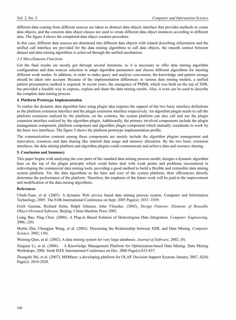
Vol. 2, No. 2 Computer and Information Science
100
different data coming from different sources are taken as abstract data objects interface that provides methods to create data objects, and the concrete data object classes are used to create different data object instances according to different data. The figure 4 shows the completed data object creation procedure. In this case, different data sources are abstracted into different data objects with related describing information and the unified call interface are provided for the data mining algorithms to call data objects, the smooth contact between dataset and data mining algorithms is achieved through the unified mechanism. 3.4 Miscellaneous Functions Get the final results are mostly got through several iterations, so it is necessary to offer data mining algorithm configuration and data sources selection to adapt algorithm parameters and choose different algorithms for meeting different work modes. In addition, in order to make query and analysis convenient, the knowledge and pattern storage should be taken into account. Because of the implementation differences in various data mining models, a unified pattern presentation method is required. In recent years, the emergence of PMML which was built on the top of XML has provided a feasible way to express, explain and share the data mining results. Also, it even can be used to describe the complete data mining process. 4. Platform Prototype Implementation To realize the dynamic data algorithm base using plugin idea requires the support of the two basic interface definitions as the platform extension interface and the plugin extension interface respectively. An algorithm plugin needs to call the platform extension realized by the platform, on the contrary, the system platform can also call and use the plugin extension interface realized by the algorithm plugin. Additionally, the primary involved components include the plugin management component, platform component and algorithm plugin component which mutually coordinate to work by the basic two interfaces. The figure 5 shows the platform prototype implementation profile. The communication contents among these components are mainly include the algorithm plugins management and innovation, resources and data sharing like internal data usage and memory allocation. By the two basic extension interfaces, the data mining platform and algorithm plugins could communicate and achieve data and resource sharing. 5. Conclusion and Summary This paper begins with analyzing the core parts of the standard data mining process model, designs a dynamic algorithm base on the top of the plugin principle which could better deal with weak points and problems encountered in redeveloping the commercial data mining tools, providing a good method to build a flexible and extensible data mining system platform. Yet, the data algorithms as the base and core of the system platform, their efficiencies directly determine the performance of the platform. Therefore, the emphasis of the future work will be paid to the improvement and modification of the data mining algorithms. References Chieh-Yuan, et al. (2005). A dynamic Web service based data mining process system. Computer and Information Technology, 2005. The Fifth International Conference on Sept. 2005 Page(s): 1033 -1039. Erich Gamma, Richard Helm, Ralph Johnson, John Vlissides. (2002). Design Patterns: Elements of Reusable Object-Oriented Software. Beijing: China Machine Press 2002. Liang Bao, Ping Chen. (2006). A Plug-in Based Solution of Heterologous Data Integration. Computer Engineering, 2006, (20). Meilin Zhu, Chongjun Wang, et al. (2002). Discussing the Relationship between XML and Data Mining. Computer Science, 2002, (10). Weining Qian, et al. (2002). A data mining system for very large databases. Journal of Software, 2002, (8). Xingsen Li, et al. (2006). A Knowledge Management Platform for Optimization-based Data Mining. Data Mining Workshops, 2006. Sixth IEEE International Conference on Dec. 2006 Page(s):833-837. Zhongzhi Shi, et al. (2007). MSMiner: a developing platform for OLAP. Decision Support Systems January 2007, 42(4) Page(s): 2016-2028.

Computer and Information Science May, 2009
101
Figure 1. Data Mining Flow Model
Figure 2. Data Mining Platform Structure
DMAlgorithmManager
Key Value
AlgorithmName1 Algorithm1
AlgorithmName2 Algorithm2
... …
DMAlgorithm
String dmAlgorithmName
File dmAlgorithmFile
String dmAlgorithmType
String dmAlgorithmEntry
String algorithmEntryParameters
Figure 3. Hash Mapping of Algorithm Manager and DMAlgorithm
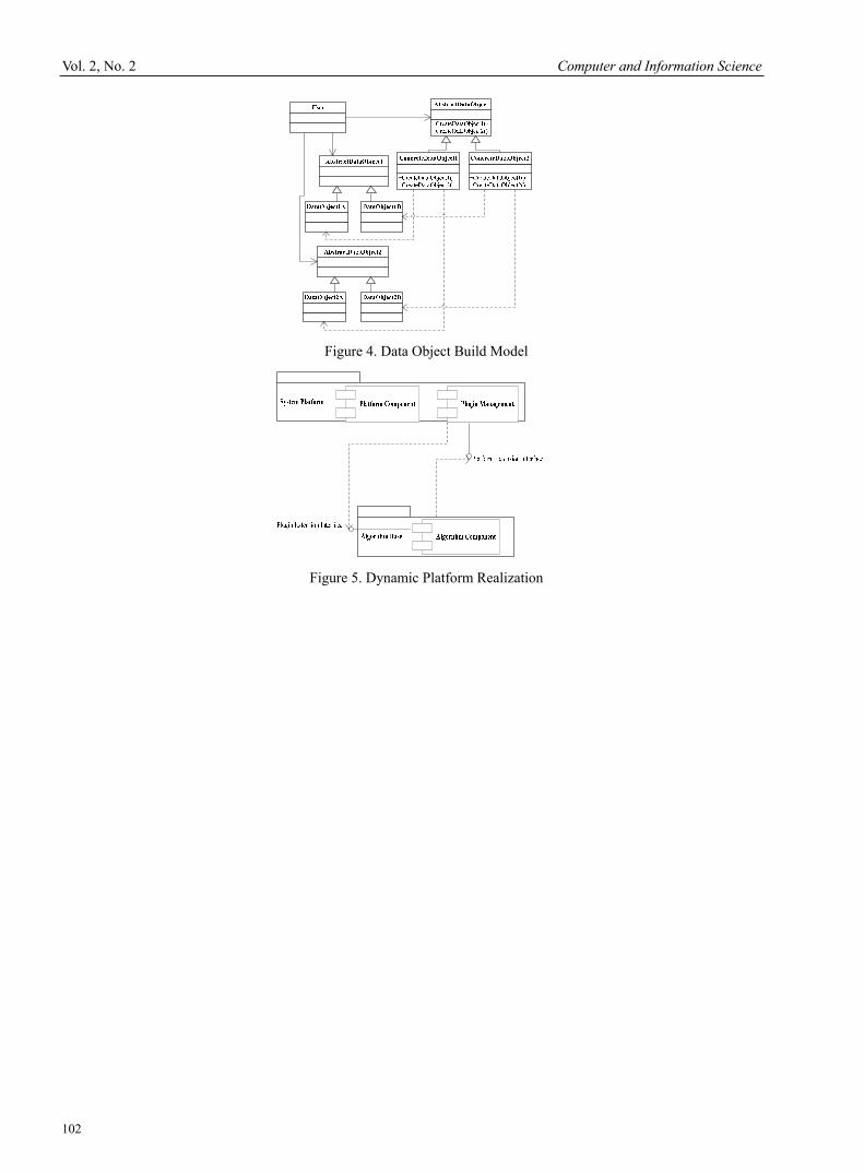
Vol. 2, No. 2 Computer and Information Science
102
Figure 4. Data Object Build Model
Figure 5. Dynamic Platform Realization

Computer and Information Science May, 2009
103
Study on the Data Mining Algorithm
Based on Positive and Negative Association Rules Jingrong Yang & Chunyu Zhao
The Engineering & Technical College, Chengdu University of Technology, Chengdu 614007, China Tel: 86-833-383-2599 E-mail: [email protected]
Abstract In this article, we systematically, deeply and comprehensively analyzed and studied the association rule data mining technology, and induced, analyzed and researched the typical mining algorithms of association rule and their basic principles, and objectively compare the differences among various algorithms. We used to correlation to measure the relations among item sets, and gave the computations of support level and confidence level of negative association rule based on traditional association rules, and analyzed and researched the operation principle and implementation approaches of this algorithm. Through the demonstration test of the algorithm, the results indicated that the algorithm was effective. Keywords: Data mining, Association rule, Correlation, Positive and negative association rules 1. Introduction Traditional database application emphasizes the online transaction processing (OLTP), and its main task is to exert the online transactions and inquiry processing. The quick increasing speed of the commercial database which intention is OLTP requires that the data mining technology which could offer the support information for the decision-making develops quickly, i.e. the online analysis processing (OLAP) could acquire and utilize information from the database. At present, the domestic researches about data mining mainly concentrate in the optimization and improvement of the algorithm. Based on former research results, we study the association rule, i.e. the negative association rule, from another view, and make it combine with traditional association rule to form the positive and negative association rule, which will make the theory of association rule more perfect. 2. Basic concept of association rule The association rule is one of very important rules which the data mining technology can apply, and it is used in the interest association among item sets of large amount of data, for example, the association rule mining can be used to find the association among different commodities (items) in the transaction database. Suppose I=i1 i2,…, im is the set of item, and suppose the data D relative to the task is the set of the transaction in the database, and each transaction T is the set of item, and T⊆ I. Each transaction has one identifier which is called as TID. Suppose X is the set of item in I, and it is called as the item set, and the transaction T contains X when and only when X⊆T. The association rule is the formula like X⇒ Y, and X⊆ I, Y⊆ I and XI Y=Φ. The rule X⇒ Y comes into existence in the transaction D, and it has the support level, s (support), and when and only when the proportion that D contains the transactions of XUY is s, i.e. s=support(X⇒Y) = P(XUY) = |T|X U Y ⊆∈T∧ T∈D |/|D| The rule X⇒ Y comes into existence in the transaction D, and it has the confidence level, c (confidence), and when and only when the proportion that D contains the transactions of X is c, i.e. C=confidence(X⇒Y) = p(Y/X) = T| X U Y ⊆T∧ T∈D |/|T|X ⊆T∧ T∈D| The set of item is called as the item set. The item set contains k items is called as k-item set, for example, printer, computer is a 2-item set. The occurrence frequency of the item set is the amount of transaction containing the item set, which is called as the frequency of the item set, the support count or the count. The item set fulfills the minimum support, min_sup, when and only when the occurrence frequency of the item set exceeds or equals the product of min_sup and the amount of transactions in D. the item set fulfilling min_sup is called as the frequent item set. The frequent item set containing k items is called as the frequent k-item set which is generally noted as Lk. The association rules which fulfill the min_sup and min_conf (minimum confidence level) synchronously are called as the strong rules.

Vol. 2, No. 2 Computer and Information Science
104
3. Mining algorithm of positive and negative association rules Traditional association rule (AR) has the form of A⇒B, and it is used to mine the association relation among the item sets in the database of consumer transaction, and it was first proposed by R. Agrawal et al in 1993, and he proposed a sort of quick algorithm in 1994. As one important complement of the association rule of A⇒B, the association rules with three forms such as A⇒ B, A ⇒B, A ⇒ B are studied in this article, and they are called as the negative AR (NAR). We will give a sort of simple and effective method which was used to compute the support level and the confidence level of NAR only by relative information of positive association rule, and an algorithm which could synchronously mine positive and negative association rules. The difference with existing algorithms is that the algorithm in this article can not only synchronously mine the positive and negative association rules in the frequent item set, but test and delete the inconsistent rules. 3.1 Computations of support level and confidence level in negative association rule The confidence level (c) of the rule A⇒B in the transaction database D means the ratio of the amount of transaction containing A and B and the amount of transaction containing A, i.e. c(A⇒B). The negative association rule contains non-existing-items such as A and B, and because it is difficult to directly compute their support level and confidence level, so we give following theorems and computation methods. Theorem 1 Suppose A, B⊂ I, A∩B=Φ, so we have a. s(A)=1-s( A); b. s(A B)=s(A)∪ -s(A B);∪ c. s( A B)=s(B) ∪ -s(A B);∪ d. ( A B)=1 ∪ -s(A)-s(B)+s(A B).∪ To prove this theorem, we need to re-denote the support level and the confidence level from the view of set, i.e. changing the set operation of item set into the set operation of transaction set, which can better apply some theorems and characters and be easy to be understood. Suppose As denotes the set of transactions containing the item set A, and its base |As| is the amount of transaction in As. In the same way, suppose Bs denotes the set of transactions containing the item set B, and its base |Bs| is the amount of transaction in Bs. The database D is the set of all transactions in the database, i.e. the total set which is denoted by D, its base |D| is the amount of all transactions, so the corresponding conversions are a. s.count(A B)=|As∩Bs|;∪ b. s(A)=s.count(A)/|D|=|As|/|D|; c. s(A B)=s.count(A B)/|D|=|As∩Bs|/|D|;∪ ∪ d. c(A⇒B)=s(A B)/S(A)=|As∩Bs|/|As|.∪ Deduction 1 Suppose A,B,I,A∩B=Φ, so we have a. c(A⇒ B)=(s(A)s(A B))/s(A)=1 ∪ -c(A⇒B); b. c( A ⇒B)=(s(B)-s(A B))/(1∪ -s(A)); c. c( A ⇒ B)=(1 -s(A)-s(B)+s(A B))/(1∪ -s(A))=1-c( A ⇒B). According to Theorem 1 and the definition of the confidence level, we can easily prove Deduction 1 which can be used to compute the confidence level of the negative association rule. 3.2 Algorithm of mining positive and negative association rules In the algorithm, suppose that the frequent item set has been solved and stored in the set L. Algorithm 1 Mining_PAR&NAR Input L: frequent item set; min_conf: minimum support level; Output: The set of positive and negative association rules AR; a. AR=Φ ; b. // generate the positive and negative association rules in L. For any itemset X in L do
for any itemset A B=X and A∩B= Φ do∪
corr=s(A B)/(s(A)s(B))∪

Computer and Information Science May, 2009
105
if corr>1then // generate the rule of A⇒B and the rule of A ⇒B
if c(A⇒B)≥min_conf then AR=AR A∪ ⇒B; if c( A ⇒ B)≥min_conf then AR=AR A∪ ⇒ B;
if corr<1 then generate the rule of A∥ ⇒B and the rule of A ⇒B
if c(A⇒ B)≥min_conf then AR=AR A∪ ⇒ B; if c( A ⇒B)≥min_conf then AR=AR A∪ ⇒B;
c. Return AR. To validate the validity of Algorithm 1, we do a test in the synthetic data, and the test is performed under the environment of Celeron 2.5, 256RAM, WIN2000, VC++. There are experimental data containing 200 transactions, and the maximum item set number is 5. Suppose that min_supp is 0.20, min_conf is 0.40, and Table 1 lists the comparison of experiment results of two algorithms. From Table 1, the positive association rule number obtained by Algorithm 1 is significantly less than the positive association rule number obtained by traditional Apriori algorithm, which indicates some inconsistent rules have been deleted, and many negative association rules have been mined, which indicates Algorithm 1 is effective. 4. Research of P-S interest in positive and negative association rules Only the rule of A⇒B accords with the condition of supp(AUB)-supp(A)supp(B)≥miniuterest>0, it is interesting, but for negative association rule, supp(AUB)-supp(A)supp(B) may be less than 0, so we use its absolute value as the condition, i.e. only if the rule of A⇒B accords with the condition of |supp(AUB)-supp(A)supp(B)|≥mininterest, it is interesting. What relations exist in the minimum interests of four sorts of association rule? Theorem 2 If |supp(AUB)-supp(A)supp(B)|≥mininterest, so (1) |supp(AU B) -supp(A)supp( B)| ≥ mininterest; (2) |supp( AUB) -supp( A)supp(B)| ≥ mininterest; (3) |supp( AU B) -supp( A)supp( B)| ≥ mininterest. Theorem 2 indicates that only if the mini-interest is reasonably set up, some rules without interest can be avoided effectively, and four sorts of association rule can be restricted by one minimum interest P. When studying the positive and negative association rules at the same time, the problem of conf( A =>B)>conf(A=>B)>min_conf may occur, so the application of correlation is the effective method to solve this problem. The correlation of association rule can be measured by supp(AUB)/(supp(A)supp(B), where s(A)≠ O,s(B)≠ 0. In fact, if we improve the P-S interest little, it can be used in the correlation judgment of association rules, i.e. using corr(A,B)=supp(AUB)-supp(A)supp(B) to measure the correlation. There are three possible instances for corr(A,B). (1) If corr(A,B)>0, so A and B are positively correlated, i.e. transaction A occurs more, transaction B occurs more too. (2) If corr(A,B)=0, so A and B are independent each other, the occurrence of transaction B is independent of transaction A. (3) If corr(A,B)=0, so A and B are negatively correlated, i.e. transaction A occurs more, transaction B occurs less. Theorem 3 If corr(A,B)>0, so (1) corr( A,B)<0;

Vol. 2, No. 2 Computer and Information Science
106
(2) corr(A, B)<0; (3) corr( A, B)> 0; the results will be contrary. Theorem 3 indicates that the rule of A =>B (or A=> B) and A=> B(or A=>B) can not be the effective rules simultaneously, so the dissociable rules will be effectively prevented. References Dong, Xiangjun, Song, Hantao & Jiang, He et al. (2004). Minimum Interestingness Based on Method for Discovering Positive and Negative Association Rules. Computer Engineering and Applications. No.27. P.24-25, 31. Dong, Xiangjun, Wang, Shujing & Song, Hantao et al. (2004). Study on Negative Association Rules. Transactions of Beijing Institute of Technology. No.11(24). P.978-981. Huang, Jin & Yin, Zhiben. (2003). Improvement of Apriori Algorithm for Mining Association Rules. Journal of University of Electronic Science and Technology of China. No.32(1). P.76-79. Lu, Jingli, Xu, Zhangyan & Liu, Meiling et al. (2004). An Improved Algorithm for Identifying Negative Association Rules. Journal of Guangxi Normal University (Natural Science Edition). No.22 (2). P.41-46. Peng, Mugen. (2002). The Database Technology and Its Implementation. Beijing: Electronic Industry Press. Table 1. Comparison of association rule number
Algorithm Association rule number
Apriori +365
+282 Algorithm 1
-603

Computer and Information Science May, 2009
107
Temperature Measurement and Control System
Based on Embedded WEB Limin Cai
College of Physics and Information Engineering, Jianghan University Wuhan 430056, China
Tel: 86-27-8422-6780 E-mail: [email protected]
Abstract The Web-based Distributed Measurement and Control is becoming more and more prevalent in recent years. With programmable 1-wire Digital Temperature Sensor DS18B20, an embedded system is used as the field processing unit. With application mode of B/S, a remote temperature-measurement and control system is designed by embedded Web on embedded system. The experimental result shows that the system has high reliability and precision. Keywords: Embedded WEB, DS18B20, Embedded system, HTTP, Internet 1. Introduction Along with the rapid development of the technology of computer, network and communications, equipment test and control are gradually shifting from field test to the network, the original field operations are replaced by the distributional remote real-time control. As the Ethernet, the internet and the embedded system application technology starts to apply to the distributional long-distance real-time control field, embedded Web system has attracted increasing attention for its superior performance. The kernel of the embedded Web system is the embedded system, it operates not only for the field data acquisition, but also as the embedded Web server, tests the network by sending and receiving data to and from other equipments, realizing the distributional long-distance real-time control function. Compared to the traditional ways, it realizes wider usages, higher rates and more open to users, much easier to connect the system to the intranet and internet, therefore, the embedded Web system are recognized by more and more people worldwide. A remote temperature measurement and control system directly to the Internet, we need a sort of gateway between temperature measurement and control system and the Internet. There can be many possible solutions to this problem, but these can be boiled down to the following three categories. 1) Field devices integrated with web server One possible way of connecting field devices to the Internet is to fit an entire web server into the field device. But, most of the microcontrollers do not have enough computing power and memory for the web server. 2) PC as a gateway Most of the field devices connected to the Internet are using PC or workstation as a gateway to the Internet. The devices send minimum required information such as the status of the sensor to the PC through it's communication ports(usually RS-232) and the web server running on the PC collects the information from the device and makes HTML pages and sends the HTML page back to the web client requesting the page. But, the PC is too big and expensive to be used for this purpose. 3) Small network computer Other way of connecting field devices to the Internet is using a small network computer, It is a small, inexpensive web server. But it is too expensive to be used for a remote temperature measurement and control system. The embedded system, which emphasizes on the applications, with the computer technology as its foundation, based on necessary software and hardware, realizes a special system with strict qualifications like high reliability, low cost, low power consumption. It is also the next generation of the computer technology, the communication, the semiconductor technology, the microelectronic technology, the sound/image data transmission technology and so on, so it can be widely used in many fields, like electrical appliances, industry, communication, national defense. In this paper the field temperature sensor is the programmable 1-wire Digital Temperature sensor DS18B20, the PHILIPS Corporation

Vol. 2, No. 2 Computer and Information Science
108
LPC2210 with ARM7TDMI-S core as its microprocessor, realizes the information interacts with the client by HTTP protocol, the user transmits the parameters and the request information by HTTP to the embedded Web server, and the server controls the sensor state according to the user parameters and the field temperature; at the same time, it returns the terminal data back to the browser, for the long-distance user monitoring, in this way it realizes embedded Web temperature control system with B/S structure. A sample has been carried out by this design, which meets all requirements and works perfectly. 2. Systems solutions and principle of work The overall structure of the temperature measurement and control system based on embedded WEB is shown in Figure 1. The embedded Web server is located at the monitor field, the temperature sensor, heater stick and the LCD monitor and so on communicates with the embedded microprocessor I/O ports. The user’s browser goes on the Internet and to the embedded Web server. When it’s working, the user can login the embedded Web server, set the parameters on browser and can see the values of field’s temperature. In the field, the DS18B20 passes the data by I/O to the microprocessor, the microprocessor control the heating rod condition pursuant to the parameters and values of field temperature measured; all these data can be displayed on the LCD monitor, as well as the browser. In this way the long-distance temperature monitoring based on B/S structure is realized. 3. Hardware designs For the hardware system structure, see Figure 2. On the hardware side, the embedded system uses the LPC2210 processor from PHILIPS Corporation with the ARM7TDMI-S core as its processor. The LPC2210 is a 16/32 ARM7TDMI-S CPU micro controller supporting real-time simulation and the embedded track. The application which was limited to strict code scale can still work by using 16 Thumb instructions to reduce the code scale by 30%, while the performance loss is actually very little. With low power consumption, several 32 bit timers, 8 Channel 10 bit ADC, PWM channels and up to 9 external interrupts, this microcontroller is particularly suitable for industrial control, medical system, network access control, etc. LPC2210/2220 can provide up to 76 GPIO by bus configuration. With a wide range of serial interfaces inside, it is also very suitable for gateways, protocol converters and embedded soft modems as well as many other general-purpose applications. The network chip is RTL8019, the LCD display is SMG240128, the programmable 1-wire Digital Temperature sensor DS18B20 works for temperature Data Acquisition, the data in or out of DS18B20 only to need a single line for read/write, the temperature transformation power originates from the data bus, the main bus itself can also supply power to the DS18B20 without external power source. It’s easy to read temp as 9-12 numbers by programming. The embedded system communicates with the sensor by GPIO port. 4. Software Designs Software system structure is shown in Figure 3. The real-time operating system is µC/OS-II. µC/OS-II is a complete, portable, scalable, ROMable, multi-tasking, fully-preemptive real-time kernel. Most of µC/OS-II is written in highly portable ANSI C, containing a small part of assembly codes, which enables the OS to be ported to a large number of processors by modifying its codes. ZLG/IP is an embedded system development oriented TCP/IP protocol stack, developed by Guangzhou Zhouligong MCU development Ltd. co, as well as an important member of ZLG middle wares. ZLG/IP provides IP switch function in the Internet, and it is an embedded TCP/IP protocol stack software with high performance. It realizes a parallel re-entry multi-tasks protocol stack by the µC/OS-II real-time operating system signal mechanism, totally written by ANSI C, supporting many kinds of CPU as µC/OS-II. ZLG/IP is clear in structure, easy to upgrade and be modified. It connects to the network by network driver downward, provides HTTP service upward. The data of temperature is processed by HTTP between client browser’s HTMLS. 4.1 µC/OS-II port Most of µC/OS-II is written in highly portable ANSI C, with target microprocessor specific code written in assembly language. Assembly language is kept to a minimum to make μC/OS -II easy to port to other processors. For instance, µC/OS-II can only work in the assembly language when reading/writing processor or registers. So the processor has to satisfy the following requests: 1) Processor’s C compilers can produce re-entry code. 2) it can enable/disable interrupt in the program. 3) Processor supports interrupt, and can produce fixed time interrupts (usually between 10Hz and 1000Hz). 4) Processor can hold the some data in the hardware stack. 5) Processor has stack pointer and other instructions on restore/load CPU register/stack. It’s all implemented in LPC2210. In fact, µC/OS-II may be regarded as simply a multi-tasks scheduler. Some system services relating to the multi-task operating system are added and its 90% code is in the C language, which may be

Computer and Information Science May, 2009
109
ported directly to processor with C language compiler. The ported work mainly concentrates on the multi-task switch, for this part of code works is used to preserve and restore the CPU scene, therefore we cannot use the C language but the assembly language to complete. The µC/OS-II be ported process, needs to 3 files related to the ARM architecture, related code in OS_CPU.H with the processor and the compiler, the assembly code in OS_CPU_A related to the processor, the 6 functions in OS_CPU_C related to the µC/ OS-II. 4.2 Implement of HTTP Server The HTTP protocol is the application layer object-oriented protocol above the TCP/IP protocol. The HTTP protocol is the standard Web application protocol, which is used by the Web server to communicate with the browser. HTTP had stipulated the standard transmission and the processing request way, transmission message format and control information. The HTTP protocol has two functions, to transmit file and interact. The HTTP protocol is based on request/reply mechanism, the client requests to the server, and the server returns the file object back to the client as response. Every HTTP interaction is from the client to the sever in this way, and then backward as the response. The form of the HTTP request is very simple, request and response is all expressed by simple ASCII code. The server response to the customer request, the server resolves the client request, then acts the corresponding behavior according to the method, and transmits a response to the client. The response form is similarly very simple, including a state code indicating request successfully (for example, if not successful, it will show the reason), and the object set. Afterwards, the server then will transmit any data requesting. After the data transmission, the server finishes this connection. As the Web server application, the HTTP protocol mainly resolves the client side requests; here we realizes the simple HTTP protocol, mainly analyzing the GET way, thus we can obtain the parameter and the request from the client, then return the information in the HTML form onto the client browser. The HTTP protocol is above the TCP/IP protocol; TCP/IP protocol is the connection oriented. The TCP protocol stipulates that, before the data transmission, the TCP connection establish process must be used to establish connection between two nodes. With successful connection, it then carries on the data transmission. The TCP connection interrupt process must also be used for connection termination. The SOCKET connection is TCP/IP API. We adopt the TCP communication here. The TCP programming is divided into two kinds, the server way and the client way. The server way needs to listen to the connection, and it can process data only after establishing connection with the client. The client way is to connect the server initiatively and it processes data after establishing connection, too. ZLG/IP provides standard BSD socket. The socket programming works with the client/server mechanism. A complete socket network application is shown in Figure 4. The relationship between client and the server is not asymmetrical. The server starts first, then client requests on own initiative at some time, the server replies passively. The client program first calls socket(), this function produces socket for various subsystems connection, and one ID number for each connection, then initializes a socket connection , sets its ID number as well as the sever end IP address and port number, and takes it as the parameter of function connect(), calling the connect() function to connect the sever side initiatively. After the establishment of connection between the client end and the sever end, it can send (write) or receive (read) data. 4.3 Data Acquisition The field temperature sensor is programmable 1-wire Digital Temperature sensor DS18B20, it links to a pin of GPIO on LPC2210. LPC2210 orders and receives the temperature value through this pin, processes digital filter and two-decimal transformation. DS18B20 will directly output the temperature value as digital, it has only three effective pins: DQ (data), VDD (power supply) and GND . DS18B20 reads and transmits information in the DQ line with 5K pull-up resistance. It can run without power supply and it can also links to one 3v to 5.5v power supply in the VDD line. DS18B20 has ROM and RAM internally, an independent sequence number is restored in its ROM, thus many DS18B20 can work at the same time on a bus. The process of visiting DS18B20 through the single bus is as follows: initialize DS18B20, then write the ROM operational code and the memory operation code and finally read the data. According to the DS18B20 initialization timing, write timing and read timing, we program separately 3 sub-procedures: Init_DS18B20 as the initialization subroutine, WriteOneChar() as write (order or data) subroutine, ReadOneChar() as read subroutine, all data read-write starts from the lowest bit. 4.4 Experiment Result As regarding to the temperature-measurement and control system based on embedded Web, the experiment on the internet indicates that, its measuring accuracy and the control speed meet the requirements , It has an operating temperature range of –55°C to +125°C, and is accurate to ±0.5°C over the range of –10°C to +85°C. 5. Conclusion Temperature measurement and control system based on embedded Web contains the 1-wire Digital Temperature sensor DS18B20 as its measurement device and the embedded microprocessor LPC2210 as its core, realizing a remote control system based on B/S structure. The experiment on the internet indicates that, the measuring accuracy and the control

Vol. 2, No. 2 Computer and Information Science
110
speed meet the requirement. Of course, the UI in the client end appears a little simple, to which we will make further improvements. References DS18B20 Programmable Resolution 1-Wire Digital Thermometer http://www.maxim-ic.com/quick_view2.cfm/qv_pk/2812 Jan. 2008 Wang Tianmiao. The embedded system design and the example, Beijing: Tsinghua University Press, 2003. pp. 4-5. Zhou Ligong. ARM embedded system foundation course. Beijing: University of Aeronautics and Astronautics publication 2005.pp. 132~133
Embedded Web Heater
Temperature
LCD
Brows Intern
Figure 1. System Structure Chart
LPC2210 PHILIPS
JTAG
Keyboard Reset
FLASH SDRAM
RJ45
RTL8019A
LCD
I/O
Figure 2. Hardware System Structure
µC/OS-II
HTTP
ZLG/IP
Driver
Sensor
HTM
L
Figure 3. Software System Structure Chart

Computer and Information Science May, 2009
111
connect() Connect
Request
Answer
Socket()
bind()
listen()
read()
write()
close()
Socket()
write()
read()
close()
accept()
Server Client
Figure 4. socket application flowchart

Vol. 2, No. 2 Computer and Information Science
112
A Model of Intrusion Tolerant System Based on Game Theory Huawang Qin, Yuewei Dai & Zhiquan Wang
School of Automatization, Nanjing University of Science and Technology Nanjing 210094, China
E-mail: [email protected] Abstract Intrusion tolerance is the rising third generation technology of network security. For the shortcomings of existing models, a model of intrusion tolerant system based on game theory is proposed. The intrusion tolerant system and the intruder are seen as the two sides of the game. The income functions of the two sides are designed basing on some given concepts. Through quantifying and analyzing the income functions, the optimum strategies of the intrusion tolerant system and the intruder are obtained, and the Nash equilibrium of the game system is achieved finally. The results of analysis show that, this proposed model of intrusion tolerant system is consistent with the practical system. Keywords: Intrusion tolerance, Network security, Game theory, Nash equilibrium 1. Introduction The security of network system has been a topic of concern with the intrusion incidents occurring continually. Although the firewall and intrusion detection software can protect the network effectively, the practices have show that no firewall or intrusion detection software can guarantee the network from being intruded absolutely. Under such circumstance, intrusion tolerance was born. Intrusion tolerance is the third generation technology of network security. The concern of intrusion tolerance is not how to defend or detect the intrusion, but how to mask or restrain the intrusion when the network has been intruded. Intrusion tolerance can guarantee the confidentiality and integrality of data as well as the usability of service when the network has been intruded. Intrusion tolerance is a rising research topic in the field of network security, and it has broad application future. With the promotion of the USA’s OASIA and the European Union’s MAFTLA, the technology of intrusion tolerance has developed rapidly in recent years. For the study of domestic and foreign academia, the modeling(Goseva P. K., Wang F., & Wang R, 2001)(Peng W. L., Wang L. N., & Zhang H.G, 2005)( Cui J. S., Wang L. N., & Zhang H. G, 2004), security analysis(Madan B. B., Goseva P. K., Vaidyanathan K., & Trivedi K. S, 2004)( Yin L.H., & Fang B.X, 2006)( Singh S., Cukier M., & Sanders W. H, 2003), and design method(Jing J. W., & Feng D. G, 2002)( Castro M., & Liskov B, 2000)(Liu P, 2002)( Arsenault D., Sood A., & Huang Y, 2007) have all acquired abundant results. The modeling of intrusion tolerant system is the pivotal and basic work for studying the technology of intrusion tolerance. Goseva et al. proposed a model of intrusion tolerant system based on the conversion of multimode (Goseva P. K., Wang F., & Wang R, 2001), and classified the work states of intrusion tolerant system typically. Peng et al. designed a model based on the finite state automaton machine (Peng W. L., Wang L. N., & Zhang H.G, 2005), and described the dynamic property of intrusion tolerant system. Cui et al. gave a model based on resource and control (Cui J. S., Wang L. N., & Zhang H. G, 2004), and the model can describe the corresponding properties when the intrusion tolerant system has been intruded in parallel. Although these proposed models can describe the properties of intrusion tolerant system from some sides commendably, they still have the following shortcomings. (1) These models only describe the property of intrusion tolerant system, and not take into account the behavior of intruder. So the description of the models for the intrusion tolerant system is not comprehensive. (2) These models do not analyze the cost and reward of intrusion tolerance. However, in order to design a cost-effective intrusion tolerant system, it is necessary to evaluate the cost and reward of intrusion tolerance. (3) These models are lack of the quantitative methods, and only describe the intrusion tolerant system roughly through qualitative analysis. For the above three problems, a model of intrusion tolerant system based on game theory is proposed in this paper. The intrusion tolerant system and the intruder are seen as the two sides of game. The two sides both want to obtain the larger reward through smaller cost, so as to obtain the maximal income. In the proposed model, the optimum strategies of the intrusion tolerant system and the intruder are obtained through quantifying their incomes, and the Nash equilibrium of

Computer and Information Science May, 2009
113
the game system is achieved lastly. 2. The optimum strategy of intrusion tolerant system 2.1 Tolerance cost and tolerance probability Definition 1 Tolerance cost: all the expenditures that the intrusion tolerant system needs on hardware, software and wage for the function of intrusion tolerance are called tolerance cost. The tolerance cost includes three parts: hardware expenditures, software expenditures, and wage expenditures. The hardware expenditures are used to buy and maintain the additional agents, servers, memories, communications equipments etc; the software expenditures are used to buy and maintain the additional operating systems, encryption and authentication software, communications software, and other application software etc. the wage expenditures are the payment for the employees who design and maintain the intrusion tolerant function. Definition 2 Tolerance probability: for some special tolerance cost, the statistical probability that the intrusion tolerant system can tolerate the intrusion and avoid the losses when it has been intruded is called tolerance probability. The tolerance probability is used to describe the performance of intrusion tolerance quantitatively. An intrusion tolerant system can increase its tolerance probability through increasing redundancy, enhancing the performance of hardware and software, and improving the skill of design and maintenance engineers. Obviously, these measures will all increase the tolerance cost of the system. For an intrusion tolerant system which is designed commendably, it can be considered that its tolerance probability increases monotonously with its tolerance cost increasing, that is, larger tolerance cost corresponds to larger tolerance probability. If the tolerance cost nears infinity, we can consider that the redundancy of the system is infinite, the performance of hardware and software is perfect, and the skill of engineers is perfect too. Under such circumstance, it can be considered that the system can tolerate any intrusion, that is, the tolerance probability of the system is 1. If the tolerance cost is 0, we can consider that the system has no redundancy, and the hardware, software as well as the design technology all have no function for intrusion tolerance. In this case, it can be considered that the system can not tolerate any intrusion, that is, the tolerance probability is 0. For example, in the typical (t, n) threshold intrusion tolerant system, a data is divided into n shadows and distributed to n different servers. Any t or more servers can recover the data, but any fewer than t servers can not recover the data. Therefore, if the number of the servers which are controlled by the intruder is less than t, the intruder can not get the data; if the number of unspoiled servers is not less than t, the system can still recover the data. Obviously, the data in the (t, n) threshold system can tolerate the intrusion on both the confidentiality and the integrality. The tolerance probability of the (t, n) threshold system can be increased through increasing the value of n and t, and enhancing the security of each server. But this will also increase the tolerance cost of the system. If the tolerance cost of the (t, n) threshold system nears infinity, then the values of n and t can also near infinity, and the security of each server will almost be perfect. Under such circumstance, the tolerance probability of the system can be considered 1 apparently. If the tolerance cost of the system is 0, then there is no redundancy in the system, that is, the data is saved in only one server. In this system, if the server is intruded by the intruder, the intruder can not only obtain the data but also destroy the data. So the data has no tolerance function for intrusion, and the tolerance probability of the system will be 0 accordingly. In practical (t, n) threshold system, the values of n and t are not decided according to some quantitative criteria, but often decided roughly according to the importance of system, the limit of cost, and the experience of deviser etc. When studying the security of the fault-tolerant control system or the network system, the exponential distribution is usually be assumed so as to adopt the stochastic modeling tools such as Markov decision process and stochastic Petri net etc. Moreover, Jonsson and Olovsson verified the exponential distribution property of the intrusion behavior in internet through special experiments (Jonsson E., & Olovsson T, 1997). In view of this, we define the relationship between the tolerance cost and the tolerance probability through exponential function.
PS = 1-e-λc C≥ 0 (1) Where, PS is the tolerance probability; C is the tolerance cost; λ is the parameter of the exponential function, it is influenced by the network’s functions, security, and physical environment etc. It can be seen from Formula (1) that, tolerance probability increases with the increasing of tolerance cost; if the tolerance cost is 0, then the tolerance probability is also 0; if the tolerance cost nears infinity, then the tolerance probability is 1. Besides, because of the property of exponential function, the tolerance probability does not change equably with the changing of tolerance cost. When the tolerance cost is smaller, its change generates greater influence on the tolerance probability; and with the tolerance cost becoming larger, its change generates less influence on the tolerance probability. For a practical intrusion tolerant system, when its tolerance cost is smaller, its performance of intrusion tolerance can be improved distinctly if its tolerance cost increases rationally, such as through increasing the redundancy, enhancing the security performance of hardware and software, optimizing the configuration, and improving the skill of engineers etc. However, when the tolerance cost of the system is larger, its performance of intrusion tolerance can not be improved clearly if its tolerance cost increases because that the redundancy, the resource of hardware and software, the configuration, and the skill of

Vol. 2, No. 2 Computer and Information Science
114
engineers etc have already achieved higher level. 2.2 The income function and the optimum tolerance cost The income of the intrusion tolerant system is influenced by the reward and the cost of intrusion tolerance. It is defined by Formula (2).
US = PAPSE-C (2) Where, US is the income of the intrusion tolerant system; PA is the probability that the intruder can intrude into the system successfully (see Definition (4) and Formula (5) in Section 3.1); PS is the tolerance probability; E is the losses when the system has been intruded and it can not tolerate the intrusion; C is the tolerance cost. When the system is intruded, the function of intrusion tolerance decreases the probability of losses, and this is the reward of intrusion tolerance. So the (PAPSE) in Formula (2) is the reward. According to Formula (1) and (2), we can obtain Formula (3).
US = PA(1-e-λc)E-C (3) The goal of optimum strategy is to make the intrusion tolerant system get maximal income. Compute the partial derivative of income function in Formula (3) for tolerance cost, we will get the tolerance cost which can maximize the income. Let
S AλC
(U ) λP E= -1 = 0(C) e
∂∂
Can obtain -1
A A*
A
λ lnλP E λP E 1C = (4)
0 λP E < 1
⎧ ≥⎪⎨⎪⎩
Therefore, in order to maximize the income of the intrusion tolerant system, the tolerance cost should equal λ-1lnλPAE when λPAE≥1, and the tolerance cost should be 0 when λPAE<1. This tolerance cost C* is called the optimum tolerance cost. The optimum strategy of the intrusion tolerant system is to make its tolerance cost equal the optimum tolerance cost. It can be seen from Formula (4) that, when λPAE≥1, the probability that the system may be intruded is larger, then the optimum tolerance cost is larger, that is, the dangerous system needs large tolerance cost; in addition, the possible losses are larger, then the optimum tolerance cost is larger, that is, expensive system also needs large tolerance cost. When λPAE<1, the possible losses for intrusion will become very small. In this case, it is always uneconomical no matter how much that the system expends for intrusion tolerance. So the optimum strategy is to do nothing for intrusion tolerance, and the tolerance cost is 0. From the above analysis, we can see that the computation result of the optimum tolerance cost C* is in accord with the actual system. 3. The optimum strategy of intruder 3.1 Intrusion cost and intrusion probability Definition 3 Intrusion cost: in order to intrude into one network system, the intruder’s expenditures for buying intrusion tools and technologies, as well as the convertible expenditures for spent time and energy are called intrusion cost. Of cause, the intrusion cost may also include the legal sanction and the moral condemnation. But in reality, the probability of legal sanction for network intrusion is very small, and the intruder does not care about the moral condemnation in general, so these expenditures can be ignored. Definition 4 Intrusion probability: for some special intrusion cost, the statistical probability that the intruder can intrude into one network system successfully is called intrusion probability. The practices have shown that, the network systems in reality almost all have some vulnerabilities, and some vulnerabilities have been found but others have not been found. Besides, the existing firewall and intrusion detection software can not guarantee the network from being intruded absolutely. So in theory, the intruder always has the probability of intruding into one network system successfully. For the intruder, it can be considered that her/his intrusion probability increases monotonously with her/his intrusion cost increasing, that is, larger intrusion cost corresponds to larger intrusion probability. If the intrusion cost nears infinity, we can consider that the intruder can spend infinite time and energy on intrusion, and her/his technology for intrusion is perfect. Under such circumstance, it can be considered that the intruder can intrude into the network system absolutely, that is, the intrusion probability is 1. If the intrusion cost is 0, the intruder expends nothing for the intrusion. Obviously, the intruder can not intruder into the network system, that is, the intrusion probability is 0. In the light of Formula (1) in Section 2.1, the intrusion probability is described by Formula (5) in the following.

Computer and Information Science May, 2009
115
PA = 1-e-γD D≥ 0 (5) Where, PA is the intrusion probability; D is the intrusion cost; γ is parameter of the exponential function, it is influenced by the skill of the intruder, the environment of the network, and the security of the network etc. 3.2 The income function and the optimum intrusion cost The income of the intruder is influenced by the reward and the cost of intrusion. It is defined by Formula (6).
UA = PA (1-PS)R-D (6) Where, UA is the income of the intruder; PA is intrusion probability; PS is the tolerance probability of the intrusion tolerant system (defined in Section 2.1); R is the reward when the intruder can intrude into the system and the system can not tolerate the intrusion; D is the intrusion cost. According to Formula (5) and (6), Formula (7) can be obtained.
UA = (1-e-γD) (1-PS)R-D (7) The goal of the intruder’s optimum strategy is to get maximal income. Compute the partial derivative of income function in Formula (7) for intrusion cost, we will get the intrusion cost which can maximize the intruder’s income. Let
SAγD
γ(1- P )R(U ) = -1 = 0(D) e
∂∂
Can obtain -1
S S*
S
γ lnγ (1 - P )R γ (1 - P )R 1D = (8)
0 γ (1 - P )R < 1
⎧ ≥⎪⎨⎪⎩
D* is the optimum intrusion cost of the intruder. The optimum strategy of the intruder is to make her/his intrusion cost equal optimum intrusion cost. It can be seen from Formula (8), when γ(1- PS)R≥1, the reward that the intruder may obtain is larger, then the optimum intrusion cost is larger, that is, the intruder can expend much when the network system is profitable. Besides, the tolerance probability of the intrusion tolerant system is smaller, then the optimum intrusion cost is larger, that is, the intruder can expend much when the network is vulnerable. When γ(1- PS)R<1, the reward that the intruder may obtain will become very small. In this case, no matter how much that the intruder expends for intrusion, she/he is always uneconomical. So her/his optimum strategy is to do nothing for intrusion, and the intrusion cost is 0 obviously. From the above analysis, it can be seen that the computation result of the optimum intrusion cost D* is consistent with the actual situation. 4. The Nash equilibrium of the intrusion tolerant system and the intruder If the intrusion tolerant system is designed according to its optimum tolerance cost C*, and the intruder does not change her/his strategy unilaterally (that is, she/he does not change her/his intrusion cost D unilaterally), then the strategy of the intrusion tolerant system is the optimum strategy, and it can obtain the maximal income. Similarly, if the intruder intrudes the network system according to her/his optimum intrusion cost D*, and the intrusion tolerant system does not change its strategy unilaterally (that is, it does not change its tolerance cost C unilaterally), the strategy of the intruder is the optimum strategy. When the intrusion tolerant system and the intruder both adopt their optimum strategies, the game system achieves its Nash equilibrium. If the intrusion tolerant system changes its strategy unilaterally, for example, it increases its tolerance cost C, the tolerance probability PS will increase according to Formula (1). Then the optimum intrusion cost D* of the intruder will decrease according to Formula (8). If the intruder is sane, that is, she/he still uses the optimum intrusion cost which has decreased to intrude, her/his intrusion probability PA will decrease according to Formula (5). Then the optimum tolerance cost C* of the intrusion tolerant system will decrease according to Formula (4). Therefore, this will prompt the intrusion tolerant system to decrease its tolerance cost. Similarly, if the intrusion tolerant system decreases its tolerance cost unilaterally, then the intruder who adopts the optimum strategy will prompt the intrusion tolerant system to increase its tolerance cost. If the intruder changes her/his strategy unilaterally, for example, she/he increases her/his intrusion cost D, the intrusion probability PA will increase according to Formula (5). Then the optimum tolerance cost C* of the intrusion tolerant system will increase according to Formula (4). If the design of the intrusion tolerant system is commendable, that is, it still uses the optimum tolerance cost which has increased to design the function of intrusion tolerance, the tolerance probability PS will increase according to Formula (1). Then the optimum intrusion cost D* of the intruder will decrease according to Formula (8). Obviously, this will prompt the intruder to decrease her/his intrusion cost. Similarly, if the intruder decreases her/his intrusion cost unilaterally, the intrusion tolerant system which adopts the optimum strategy will prompt the intruder to increase her/his intrusion cost. It can be seen from the above analysis that, the balance between the intrusion tolerant system and the intruder is steady.

Vol. 2, No. 2 Computer and Information Science
116
If the two sides are all sane, that is, they do not change their strategies randomly, the normal interference will not destroy the balance. 5. The evaluation of parameters In order to obtain the optimum tolerance cost C*, the intrusion tolerant system must know the values of λ, PA, and E according to Formula (4). The values of λ and PA are influenced by the network’s application property, physical environment, vulnerabilities, and the defendable performance of the firewall and intrusion detection software etc. The value of E is influenced by the network’s importance, accessing frequency, the number of users, and the recover cost etc. For a special intrusion tolerant system, the values of λ, PA, and E can be evaluated through the Delphi method according to the practical situation. In order to compute the final tolerance expenditures, the intrusion tolerant system must know the conversion relationship between the tolerance cost C and the practical expenditure, that is, a unit of tolerance cost equals how much money. The conversion relationship can be evaluated through Formula (1) and the Delphi method. Select a special value of tolerance probability and compute the corresponding value of tolerance cost through Formula (1). Then obtain the practical expenditure of the selected tolerance probability through the Delphi method according to the practical system. Thus, the conversion relationship between the tolerance cost C and the practical expenditure can be gotten. Similarly, the intruder also needs to evaluate the values of γ, PS, R, and the conversion relationship between the intrusion cost and the practical expenditure. The intruder can adopt the same method of the intrusion tolerant system. We do not explain it in detail here. 6. Comparison to the existing models In the model proposed by Goseva (Goseva P. K., Wang F., & Wang R, 2001), the work states of intrusion tolerant system were summarized as good state, vulnerable state, active attack state, masked compromised state, undetected compromised stare, triage state, fail-secure state, graceful degradation state, and failed state. This model mainly described the static property of intrusion tolerant system. Basing on this model, Peng designed a model based on the finite state automaton machine (Peng W. L., Wang L. N., & Zhang H.G, 2005). The model described the dynamic property of intrusion tolerant system, and provided the condition and process of state transition. The model proposed by Cui classed the effect of intrusion on system resource and control (Cui J. S., Wang L. N., & Zhang H. G, 2004), and this model described the recourse state and recovery method of the intrusion tolerant system. Compared to these existing models, the main contributions of our model are that: (1) Besides the property of intrusion tolerant system, the behavior of intruder is also described in the model. So the description of the model for the intrusion tolerant system is more comprehensive. (2) The cost and reward of intrusion tolerance is analyzed in the model. In order to design a cost-effective intrusion tolerant system, this work is indeed necessary. (3) This model adopts the method of quantitative analysis, so it can provide more accurate description compared to the qualitative analysis in the existing models. 7. Conclusions Intrusion tolerance is the rising third generation technology of network security. It can provide the ultimate security guarantee for the information system in internet. The modeling for intrusion tolerant system is the basic work for studying the intrusion tolerance. For the shortcomings of the existing models, a model of intrusion tolerant system based on game theory is proposed in this paper. The intrusion tolerant system and the intruder are seen as the two sides of the game. The optimum strategies of the two sides are obtained through quantifying their income functions. The Nash equilibrium of the game system is analyzed in detail. The analysis results of the formulas in the model show that, the proposed model can reflect the actual property of the practical system. References Arsenault D., Sood A., & Huang Y. (2007). Secure, resilient computing clusters: self-cleansing intrusion tolerance with hardware enforced security (SCIT/HES). Second International Conference on Availability, Reliability and Security. Fairfax, Virginia. Castro M., & Liskov B. (2000). Proactive recovery in a Byzantine-fault-tolerant system, The 4th symposium on operating systems design and implementation. pp. 273-288. Cui J. S., Wang L. N., & Zhang H. G. (2004). A parallel model of intrusion tolerance system: RC model. Chinese Journal of Computers, 4, 500-506. Goseva P. K., Wang F., & Wang R. (2001). Characterizing intrusion tolerant systems using a state transition model, DARPA Information Survivability Conference and Exposition. pp. 211-221.

Computer and Information Science May, 2009
117
Jing J. W., & Feng D. G. (2002). An intrusion tolerant CA scheme. Journal of Software, 8, 1417-1422. Jonsson E., & Olovsson T. (1997). A quantitative model of the security intrusion process based on attacker behavior. IEEE Transactions on Software Engineering, 4, 235-245. Liu P. (2002). Architecture for intrusion tolerant database systems. Computer Security Applications Conference. pp.311-320. Madan B. B., Goseva P. K., Vaidyanathan K., & Trivedi K. S. (2004). A method for modeling and quantifying the security attributes of intrusion tolerant system. Performance Evaluation, 1, 167-186. Peng W. L., Wang L. N., & Zhang H.G. (2005). Research of intrusion tolerant system based on finite state automaton machine. MIN-MICRO SYSTEMS, 8, 1296-1300. Singh S., Cukier M., & Sanders W. H. (2003). Probabilistic validation of an intrusion-tolerant replication system. Proceedings of the International Conference on Dependable Systems and Networks. San Francisco, CA, USA, pp. 616-624. Yin L.H., & Fang B.X. (2006). Security attributes analysis for intrusion tolerant system. Chinese Journal of Computers, 9, 1505-1512.

Vol. 2, No. 2 Computer and Information Science
118
Design and Applications of the Circuit of Keyboard Display
in Detecting Axle’s Temperature System
Guilin Lu
Guangxi University of Technology, Liuzhou 545006, China
E-mail:[email protected] Abstract The technology of detecting axle’s temperature with infrared rays is a new kind of scientific product which plays an important part in the indemnity system of railway rolling stock, The circuit of keyboard and display is a man-machine interactive technology,which is composed of Chip 8279,LED digital display and correlative instruments.Coordinated by Chip 8279,LED digital display perform to read keyboard numerical values and display memory address ; power self-check is accomplished by the Voltage compare device in the circuit;the calendar clock chip 5832 makes the clock display possible. Experimental results accomplished with parameter show that the design of hardware and software is applicable to Infrared Rays System Keywords: Hot axle, Detecting axle’s temperature, The circuit of keyboard display, Man-machine interactive Preface The detecting axle’s temperature with infrared rays systemy Can find hot axle of wheel in time, so it becomes an important equipment in preventing wheel from being disconnected., and it is a new kind of scientific product which plays an important part in the indemnity system of railway rolling stock.it can detect wheel’s hot axle effectively and indemnify rolling stock against danger through making use of the theory of detecting temperature with infrared rays. The detecting axle’s temperature with infrared rays system of the Second generation has concentrated computer, optical and automatic control.it can trail inspecting running train continuously, find all kinds of hot axle faults of rolling stock automatically, alarm managers with speech.it consists of surveying station, showing station, inspecting center and Inquity Terminal.surveying station is one of major composition parts of the rolling stock’s axle temperature inspection equipment. Surveying station includes: circuit of keyboard display, wheel sensor board, the input board of axle temperature, export control plate, serial interface board and transmitting data board. GAL20V8 chips used to describe features, According to the small keyboard provided by the memory, storage registers to analyze the data to judge the work of Surveying stations, The network self-test system to form a central message and communications, the central management system carry out network management about surveying stations and showing stations, trail hot axle of passing train, forecast according to three grades: low hot, strong hot and surge hot. 1. Design of Keyboard display circuit The system hardware was design by Module, Including the CPU module, memory modules, graphics display module, A / D module, D / A module, the volume switch I / O modules, All was made by the standard size plug-in manufacturing. The functional module can be inserted any socket, In most cases, only to be replaced circuit template, they can change the function of the system, System module with the bus and the function that describes the figure 1: The modular system was denoted with code JC, JC17 case of the module's functions GAL20V8 chip is described as follows: MODULE ENCODER1 FLAG ‘-R3’; TITLE ENCODER; ENCODER DEVICE ‘P20V8S’; K2, CPU_DEN, HLDA PIN 1,2,4,8;

Computer and Information Science May, 2009
119
A15, A16, A17, A18, A19 PIN 5,11,7,6,3; MIO, INAQ, CPU_SSO PIN 9,10,13; VC PIN 14,23; TRUTH_TABLE([ K2, CPU_DEN, HLDA, MIO, INAQ, CPU_SSO, A15, A16, A17, A18, A19, JC22_18]->[ CS_DATA, STD40, CS_JC20]); input [0 ,0,0,0 ,0,0,0 ,0,0,0,0 ,0,0]->[0,0 ,0,0] ; out F0,F2…. [0,1 ,0,0,0 ,0,0,0 ,0,0,0 ,0,0]->[1,0 ,0,0]; [1,1 ,0,0,0 ,0,0,0 ,0,0,0 ,0,0]->[1,0 ,0,0]; [0,1 ,1,0,0 ,0,0,0 ,0,0,0 ,0,0]->[1,0 ,0,0]; [0,1 ,0,0,0 ,0,0,0 ,0,0,0 ,0,0]->[1,0 ,0,0]; [1,1 ,1,1,1 ,1,1,1 ,1,1,1 ,1,1]->[1,0 ,0,0]; [1,1 ,1,1,1 ,1,1,1 ,1,1,0 ,0,0]->[1,0 ,0,0]; …………………………………. [0,0 ,0,0,0 ,0,0,0 ,1,1,1 ,1,0]->[1,0 ,0,0]; [0,0 ,0,0,0 ,0,0,0 ,0,0,0 ,0,1]->[0,1 ,0,0]; [0,0 ,0,0,0 ,0,0,0 ,0,0,0 ,0,0]->[0,0 ,0,1]; [0,0 ,0,0,1 ,0,0,0 ,0,0,0 ,0,0]->[1,0 ,1,0]; TEST_VECTORS([ K2, CPU_DEN, HLDA, MIO, INAQ, CPU_SSO, A15, A16, A17, A18, A19, JC22_18]->[ CS_DATA, STD40, CS_JC20]) [0,0,0,0,0,0,0,0,0,0,0,0,0]->[0,0,0,0]; END ENCODER1 2. Circuit of keyboard display This is described in the next ABEL3.0.Its keyboard display circuit chip hardware includes two 8279 and 74LS138, hardware design to solve two questions:
The key to the elimination of jitter. Delay by the general procedures (such as delay 20ms) button on the Elimination ①of jitter.
Should be prevented by a key and a② number of key input We use software to scan lines using methods and procedures to achieve law. Which shows that the digital keyboard design sub-flow chart, Shown in Figure 2. Figure 3 of Subroutine of deal with keyboard design flow: Keyboard display circuit function, as shown in Figure 4. 3. Simulation tests In the PCB has a good system, we choose the keyboard show circuit module in the voltage comparator, In its anti-interference measures for the R8's choice ,Various components of the value of the pressure point of view:,UB>2.5V, Found to point B-to-ground resistance R13=145Ω, Therefore, to point B to measure output voltage UB, As shown in Figure 5 Choose C2=1μF, R15=150kΩ, Detected UB>2.5V. It is correct value that Note capacitor C2 and resistance the of R15. to choose PROTEL through the simulation test, Check out point B voltage, As shown in Figure 6. Soluting: jC11 pick in the R1 resistance 10kΩ, R8 resistance from 1kΩ to 10kΩ compared to arrive at the most appropriate resistance., To observe the Out4, Out2, Out1, Out3, int1, int2, int3 wave, The results shown in Figure 7. The experimental results: R8=10kΩ, Requirements for fit. 4. The keyboard show circuit module of the completion of the main functions The design of the above, the completion of the functions of monitoring power status: This keyboard display board to monitor +5 V, +12 V,-12V supply voltage changes, Power supply will be sent to the state's population 00CH-D0 ---- D5,

Vol. 2, No. 2 Computer and Information Science
120
00CH state voltage and the D0 --- D5-relationship shown in Table 2. 5. Summary Infrared detection systems show circuit keyboard software, hardware can be effectively completed the task of man-machine dialogue, Including the completion of the design and performance are: Reading of the key, the corresponding keys on the car have been reported, Self-examination revealed, Display and memory addresses, Signal is collected by Based on 8086 Microprocessor, Users of the implementation process, the exchange of information between the device and improve the original infrared temperature detection system in response to slow real-time requirements of the inadequacies of the poor. References Chen Gang, Zhang Yun. (1976). Second-generation infrared temperature detection system,1997, 6. Luguilin. (2002). China University of Science and Technology Master's Degree Essays. Wang, Ying. (1995). Temperature monitoring of railway network communications records "black box", Electrical measuring and instruments, 1995, 5.
Table 1. 00CH state voltage and the D0 --- D5-relationship
Data state Meaning
D0=1 D3=1 That is normal in Duty 5V voltage between 4.5V to 5.5V
D0=0 D3=1 voltage 5.75V said that more than exceeded the upper limit 5V
D0=1 D3=0 Voltage that is less than 4.25V, below the lower limit of 5V
D1=1 D4=1 That the value of the voltage is between 10.2V to 13.8V, normal
D1=0 D4=1 It Said over-voltage 13.8V, in excess of the maximum 12V
D1=1 D4=0 Less than that voltage 10.2V, below the lower limit of 12V
D2=1 D5=1 -12V voltage, said in-13.8V to-10.2V, normal
D2=0 D5=1 More than that voltage-13.8V, in excess of the maximum-12V
D2=1 D5=0 Voltage that is less than the above-10.2V, which is lower than the minimum-12V

Computer and Information Science May, 2009
121
M/IO
JC20(00000H~ 0FFFFH)
27512 Selected films
JC15 (30000H~ 3FFFFH) JC16(10000H~ 1FFFFH) JC19(20000H~ 2FFFFH)
address latch output
Connect data bus A19
A15 A18 A17
M/IO INAQ A16
CPU 34
CPU26
Single-oscillaReset
CPU(HLDA)
A0 A1 A2 A3 A4 A5 A6 A7
A19 A18 A17
A16
WR
1
INAQ
M/IO WR
A4
A3
A2
A7
A5 A6
RD
To the printer port,
8253 Selected films 74LS123
Serial 8251
Figure 1.
+5V

Vol. 2, No. 2 Computer and Information Science
122
order word were sent to 8279 register

Computer and Information Science May, 2009
123

Vol. 2, No. 2 Computer and Information Science
124
Figure 5. Point B test voltage map

Computer and Information Science May, 2009
125
Figure 6. B-point voltage value map
Figure 7. The results map

Vol. 2, No. 2 Computer and Information Science
126
Design of Electric Bicycle Controller Jie Cong
School of Computer Technology and Automation, Tianjin Polytechnic University Tianjin 300160, China
E-mail:[email protected] Abstract This article introduces a sort of intelligent brushless DC motor driver and its concrete application in electric bicycle, and discusses the hardware and software design scheme of the controller, and realizes the speed control, over-current protection and battery under-voltage protection of the brushless DC motor. And the experiment result indicates that the control effect is good, and it could fulfill the application requirement of electric bicycle. Keywords: LPC2114, Brushless DC motor, Electric bicycle In the day that the environment is polluted and the oil is deficient, the electric bicycle saving energy and with low noise and without pollution has been the main development direction of future vehicle in China. With the quick development of scientific technology, as one of tools to ride instead of walk in the new term, the technology of electric bicycle has been more and more mature. In past 20 years, the industry of electric bicycle has advanced rapidly. Electric bicycle possesses four performance advantages including safety, environment protection, saving energy, low maintenance and using costs, so it has large development potentials. At present, electric bicycle and electric motorcycle are very popular because of their economy and practicability. In the electric bicycle, the wheel-hub brushless DC motor is the core part. The drive of brushless DC motor generally adopts special chip. The Hall Sensor in the motor sends the phase-change signal to the control chip, and controls power switch to drive the three-phase loop by certain sequence in turn, and makes the motor run according to the requirement. But the core controller circuit is complex, and its intelligent degree is low and its reliability is bad, so we design a sort of high performance MCU LPC2114 made by PHILIPS Company as the core controller to realize many control functions such as battery percent indication, battery under-voltage protection, motor over-current protection, brake control system with power off and soft startup. 1. Performance characters of MCU LPC2114 is the 16/32 bits ARM7TDMI-S CPU based on real-time simulation and follow with embedded high-speed Flash memorizer of 128/256KB. The memorizer interface with 128bits width and the special speedup structure make 32bits code run under maximum clock velocity. The application which strictly controls the code scale can reduce over 30% of code scale by 16 bits Thumb mode, and the loss of performance is very low. The MCU has good stability, and its PWM (Pulse-Width Modulation) output function saves peripheral circuit and work time of MCU. Multiple A/D ports are integrated in the interior, which can fulfill the requirement that the system acquires many simulation signals such as rotate speed signal and current feedback signal. Abundant interrupt resource can exactly collect the phase information of motor, and realize the conversion of work mode. Multiple 32bits timers, 45 high speed GPIO and 9 marginal or level springing exterior interrupt pins will make the MCU specially be applicable in the industrial control system. 2. Work principle of brushless DC motor Because of the use of mechanical brush, a series of problem such as mechanical friction, noise, electric spark and wireless interference in the traditional DC motor, and in addition, high making cost and difficult servicing also largely limits its application range. The brushless DC motor utilizes electric commutator to replace the mechanical brush and mechanical commutator, and keeps the excellent character of brush DC motor, and eliminates the advantages of brush and commutator. Because the brushless DC motor has many advantages such as simple structure, reliable performance, high efficiency and convenient maintenance, so it is the most perfect drive motor of electric vehicle. Comparing with other motors, its main advantages include (1) good exterior character of motor, which can make the motor possess low-speed large torsion character, (2) width speed range, which can make the motor run in any rotate speed with full power, (3) high motor efficiency, and the light load will keep higher efficiency, (4) strong over-load ability, (5) good regenerated braking effect,

Computer and Information Science May, 2009
127
(6) small motor volume and light weight, (7) without mechanical commutator, and high reliability, (8) the motor control system is simpler than asynchronous motors. The brushless DC motor is usually composed by the principal part of the motor, the rotor position sensor and the power switch circuit. Figure 1 is the principle frame chart of the brushless DC motor. The Hull sensor in the figure is the rotor position sensor, and its function is to detect the position of the motor rotor, offer the position information of rotor for the electric commutator, and realize the electric commutation without touching. The inverter of the switch circuit in the figure adopts three-phase and six-beat break-over mode, and in each moment, there are two phases to be broken over, and the other phase doesn’t break over, and the winding of each phase will continually be broken over by 1200 electric angle, and the stator winding current will change phase once in each 600 electric angle. The motor character circumrotates in 3600 electric angle clockwise, and the state characters of three-route position sensor signal change from 101-100-110-010-011-001. The time that the state characters change is the time that the stator winding current will change phase. The I/O ports of MCU could be taken as the inverter upper and lower bridge arm control ports to realize the control of phase change. The inverter adopts three-phase star structure, and it is composed by six MOSFET pipes with N channels, adopts the NAND gate to realize the hardware locked logic of upper and lower arms and ensure that the upper bridge arm and the lower bridge arm will not break over in same phase. The upper bridge arm drive is composed by voltage-ascending circuit and dynatron drive circuit. When failures occur in the system, MCU locks the three-phase upper and lower bridge arms of the inverter through the control character, and the motor will stop to run. 3. Hardware design of controller The design idea includes that the system adopts three switch-type Hull sensors to be the position sensors which send the position signals of motor rotor to the I/O port of MCU. The main control chip comprehensively controls the motor according to the designed software or signals inputting from the rotor handle and the voltage and current values tested, and the MCU transmits PWM signals and control the work current of motor through the dutyfactor of PWM signals, and accordingly realize the control of speed. The system uses the inverter to realize the phase change of motor. For the control of main control chip, three Hull components in the brushless DC motor detects the position of the rotor, and transmits this signal to the MCU to produce interrupt, and the MCU inquires the table and finds out two phases which should break over at the next moment according the Hull signals, and transmits the signal to the driver bridge of MOSFET through PWM output port, so the breaking over or shutting off of MOSFET are controlled. At the same time, MCU computes the time difference between each two continual Hull signals through the counter in the chip to obtain the rotate speed of the motor, and finds out the difference between the reference speeds obtained from the rotor handle with the rotate speed, i.e. the speed error. Implement PI modulation to the speed error and output the reference current. Obtain the actual current from sampling resistance, and implement PI modulation to the current, output PWM wave to corresponding MOSFET breaking over, and modulate the motor rotate speed through changing the dutyfactor of PWM, so the double closed loops speed modulations of speed loop and current loop are realized. The whole controller takes the LPC2114 MCU as the control core, and it acquires various signals (such as the speed modulation signal, the phase change signal of Hull sensor, the voltage signal of the storage battery and the current signal of motor) to dispose according to enacted control mode, and outputs control signals. The signals acquired by the MCU mainly include following sorts. (1) The signal of Hull sensor. Three-route signal can be directly connected through resistance pulling-up and capacitance filtering, and when the corresponding Hull signals changes, the motor control unit will spring the zero-pass interrupt and phase-change accident, and close and open corresponding power MOSFET through catching the register value of signal edge, and in such cycle, the system could control the connection and breaking of three-phase winding to realize the running of the motor. (2) The Hull rotor handle signal. The rotor handle signal is a simulation voltage signal, and the rotate angle is in direct ratio to voltage. The AD sampling value of the signal corresponds with reference rotate speed, and the voltage modulation and speed modulation could be realized by modulating the chopping ratio. (3) The current signal. The main loop current signal of motor is acquired by the sampling resistance. The current signals are amplified by the operation amplifier in the chip, and the output pin connects with AD interiorly, and it can sample the current, and it also connects with one port of the comparer in the chip, and the other port of the comparer connects with the over current reference voltage, and when the current is too higher, it will spring the over-current interrupt. The peripheral circuit in this part is simple, and it only needs resistance and capacitance to realize the current amplifying sampling and over-current protection. (4) The input of accident. Under the loading condition, the instant pinnacle current will bring impact to the motor when the motor starts up or meets accidents, and the users of electric bicycle will feel uncomfortable. So input the voltage

Vol. 2, No. 2 Computer and Information Science
128
signal of current into the comparer, and when the pinnacle current occurs, the comparer outputs the negative pulse, and the hardware will automatically stop the PWM output, and spring the interrupt to dispose. (5) Other signals. The brake signal is the switch signal. When braking, the high level is effective, and when MCU reads in high level, it stops PWM outputs and implements corresponding disposal. For the under-voltage signal of the storage battery, the batter voltage meets with AD in the MCU through voltage division, and the voltage is supervised by MCU. When the battery voltage is under 43V, the system gives under-voltage signals and outputs cut-off to prevent the damage of the battery because of over-discharge. 4. System software design The software design is the important part of the system design, and it controls various functions with MCU together, and the software design in the system is composed by the main program and the interrupt service subprogram. The software design adopts modularization programming idea and the structured programming idea. The main program mainly includes the part of initialization and the part of cycle main body (seen in Figure 2). Where, the part of initialization includes the initialization of system resource and the initialization of various variables. The part of cycle main body mainly includes A/D sampling rotor handle signal and the voltage of power supply, reading brake signal to disposal and double closed loop speed modulation, and the main program will first inspect the voltage of storage batter and the brake signal in every cycle, and inspect whether there is stopping signal after every speed modulation ends. The over-current control is divided into two sorts in the program. For the type 1 of over-current, the present current exceeds the rating work current, but it is smaller than the enacted type 2 of current (failure current), and here if only properly reducing the output of PWM, the loop current will be reduced, and the disposal program is in the closed loop speed modulation. For the type 2 of over-current, the present current exceeds the enacted failure current, and the hardware forbids the output of PWM, and inspects the current continually, and when the current is smaller than the rating current, the hardware will make PWM output, and this program is in the interrupt disposal of accident, and this sort of current control method could better protect the current, avoid the situation that the current increases suddenly and stop immediately, and make the whole system more comfortable and conveniently to use. The interrupt service subprogram mainly includes voltage zero-pass interrupt, phase-change interrupt and serial interrupt. The zero-pass interrupt mainly feels the change of Hull sensor signal, and offers time interval of rotor in each 600 electric angle to measure the speed. The hardware of phase-change interrupt springs the connection and closing of the corresponding power pipe and pre-writes the register value at next phase-change. The serial interrupt program is used to communicate with the host computer. 5. Notices In the design of the electric bicycle controller, we find following problems and implement corresponding treatments to them. (1) The confirmation of sampling time for the brushless motor controller of electric bicycle The brushless motor should exactly test the position of rotor permanent magnet, and use the electric switch to switch different winding to obtain sustainable drive. The system uses three switch Hull sensors to test the position of permanent magnet relative to the stator loop, and the controller outputs corresponding control signals to drive the electric switch to supply power to the motor according to six sorts of different signals output by three Hull sensors, which is the so-called six-step phase-change method. From the principle of motor, the phase-change must be timely, or else, it will induce out-of-step of motor, and the motor noise will increase, and the efficiency will reduce and the motor and the controller will be burned. At the maximum rotate speed, electric phase changes the phase in about every 1.2ms, and according to the actual using effect, the software should detect the change of phase-change signal in about 0.12ms of the response time, and output the phase-change drive signals. Considering the phase-change signal input to the MCU is easy to be interfered, and the influence of filtering capacitance on the line, the MCU program should continually read three times at least when reading the phase-change signal, and when three times signals are completely consistent, the value can be adopted as the true value of phase-change signal, which is the phase demodulation. After the phase change signal is acquired, we compare the vale with the last value, and if they are same, there is no phase-change, and if they are different, a corresponding drive signal should be acquired according to the value to drive the electric switch. We can use the item comparison method and the table query method to realize this process. Because the table query method is quick, so we adopt the table query method in this design. (2) The smoothness problem of speed modulation for electric bicycle Because of the use of DC power supply, the speed of the motor should depend on modulating the voltage of the two ports of the motor to modulate, and the simple method is to use the PWM pulse width modulation to modulate the voltage of the two ports of motor. The work period of PWM should be selected according to the using environment of the motor, and too low frequency will produce high frequency noise that human ears can listen obviously and the

Computer and Information Science May, 2009
129
current is difficult to be control, and too high frequency will increase the switch dynamic consumption of the electric switch. The maximum width of PWM pulse will directly influence the maximum speed of motor which is decided by the voltage output by the handle. The test of handle voltage is simple, and the driver of electric bicycle will feel slowly to the speed because of the inertia, so the test of handle should not be frequent, and the AD test, power supply voltage test and brake test all need not quick speed, and it is enough to test in each 10-50ms, and for the AD test, it only needs to store the sampling values to the buffer unit in the timing interrupt, and dispose these values when the interrupt ends and returns to the main program, which will reduce the time of occupying interrupt. In the design, the electric bicycle adopts linear Hull as the handle modulation speed scheme, and the advantages of the scheme include low failure rate and without electric shock. And the disadvantage is that the voltage only changes in the range of 1.1V-4.3V under the power supply of 5V, so the software design should eliminate the zero point and multiply certain coefficient to extend dynamic range, and convert AD values in this period into the value of PWM dutyfactor. Though it adopts the stepless speed modulation, but the driver will fell smooth when it is divided into 32 classes. (3) Reducing the noise of phase-change When the electric bicycle just start up, the motor will produce large noise of phase-change, because the current is large when the motor starts up, and the motor is a sensitive load, and because the motor loop current after phase-change will not increase to the level before phase-change, so the current contrast will be very large, which will induce the drastic change of pull, and this change will induce the intense librations of motor, and we can make the PWM pulse dutyfactor achieve 100% to increase the current quickly in a period after phase-change, and reduce the librations noise. In the program design process, we need supervising the current change at any moment, and once the current achieves the level before phase-change, the PWM dutyfactor can be recovered. If the current can not achieve the level before phase-change all the while, it only needs delay more than ten PWM periods at best, i.e. if only other important works, such as phase demodulation, are not influenced. (4) The program design of locked-rotor protection To prevent the locked-rotor occurs in motor and pass same team VMOS all the while to induce damage, it is necessary to cut off the power supply of the motor in few seconds when the locked-rotor happens. The time generally is 2 seconds. And if the locked-rotor happens in the critical point of phase-change, frequent phase-change actions will occurs, which is harmful for the VMOS, so this situation should be treated as the locked-rotor. 6. Results of experiment The experimental sample motor is the 48V/350W brushless DC motor used in the electric bicycle, and the power supply is the storage battery which rating voltage is 48V used in the electric bicycle. When the load is little, the reference speed is 360r/min, and the motor speed curve from the serial port indicates that the system basically has no super modulation, and the steady state error is smaller than 2.0%, and the speed response time is about 4.5s, and the speed modulation effect is good. And the experiment result indicated that the scheme could fulfill the application requirement of electric bicycle. 7. Conclusions In this article, we introduce a sort of intelligent brushless DC motor driver based on embedded MCU LPC2114 and its concrete application in electric bicycle, and its special motor control unit simplifies the software and hardware design of the system, reduces the quantity of peripheral parts and the space of printed circuit board and the costs to the maximum extents, and the system could be applied in the present production of electric bicycle. References Cui, Wan’an. (2002). Electric Bicycle. Beijing: Machine Industry Press. Tan, Jiancheng. (1999). Special Integration Circuit of Motor Control. Beijing: Machine Industry Press. Zhang, Chen. (1996). Principle and Application of DC Brushless Motor. Beijing: Machine Industry Press. Zhou, Ligong et al. (2005). Base and Practice of ARM Microcontroller. Beijing: Beijing University of Aeronautics and Astronautics Press.

Vol. 2, No. 2 Computer and Information Science
130
Figure 1. Composing of Brushless DC Motor
Figure 2. Principal Cycle Flow Chart of Software
DC power supply
Switch circuit
Motor
Hull sensor

Computer and Information Science May, 2009
131
CRMS: An Algorithm of Classification Rule Mining
Based on Multiple Supports Chunhua Ju
Zhejiang Gongshang University, Hangzhou, China Abstract The paper presents an algorithm CRMS of classification rule mining based on multi-support, in which the frequent classification item-set tree is adopted to organize the frequent pattern sets, and array to figure the classification projected transaction subsets. The multi-support method is applied in CRMS due to the unevenly distributed classification patterns. The CRMS uses the breath first strategy assisted by the depth first strategy, and adopts pseudo projection, which makes it unnecessary to scan the database and construct the projected transaction subsets repeatedly, therefore the memory and time cost is very low, and the projecting-efficiency and scalability are higher. The CRMS algorithm can be used in the basket analysis, association rule mining for consumption behavior in the retailing industry, which supports the product layout, buying recommendation and the sale promotion. Keywords: Multi-support classification rule, Association rule mining, Frequent pattern 1. Introduction The association rule mining is an important research topic of data mining, especially the multi-support association rule mining. The current researches on classification rule mining mainly focus on the mining of the unevenly distributed and massive databases. The existing algorithms for classification rule mining with multi-support mainly focus on multi-support thresholds and scalability of store memory. They adopt the mining strategies of breadth-first, depth first, or both of them. However the breath first algorithms like Apriori(R Agrawal, R Srikant., 1994)(S Brin , R Motwani, J Ullman et al, 1997)(Lu Jie, Zhang Zhijing, 2006) are inefficient for dense datasets that contain long patterns. The depth first algorithms such as FP-Growth(J Han, J Pei , Y Yin, 2000)(Song Yuqing, Zhu Yuquan, Sun Zhihui, Chen Geng, 2003), H-Mine(J. Pei, J. Han, H. Lu, S. Nishio, S. Tang, and D. Yang, 2001) and etc. do not scale to large sparse datasets and is time-wasteful in mining dense datasets. Some algorithms like OP(Liu JQ, Pan YH, Wang K, Han J, 2002)( Liu Junqiang, Pan Yunhe, 2004) putting breath first and depth first strategies together, but using single support are not suitable for mining unevenly-distributed business databases. Although algorithms like CRM-PP(Liu Junqiang, Sun Xiaoying, Wang Xun, 2003) adopt multi-support method, they are not scalable for storage space with the limitation of memory. This paper presents a novel algorithm, multi-support algorithm CRMS for classification rules mining in business databases, which is efficient on dense databases at all levels of support threshold, and scalable to very large databases. The main contributions are: first, the paper presents the frequent classification item-set tree for constructing frequent pattern sets, and adopt both breath first and depth first strategies for rules mining, which enhance the build of frequent pattern tree. Second, it proposes an array-based format for classification tree for pseudo projection with high efficiency and low memory cost, and adopts multi-support thresholds to mine more potential and effective association rules. Finally, it gives the design and implementation of a multi-support algorithm CRMS for classification rules mining. With the comparison experiments with Apriori, FP-Growth and OP, CRMS has certain advantages in mining efficiency and scalability of the large business databases. 2. Construction of Frequent Classification Item-Set Tree 2.1 Problem Descriptions Definition 1 The classification database D=(O,I,C), in which O is the finite set of data objects, I is the set of data attributes, and C is the set of classification items. The data attribute set also known as an item set, I=i1,i2,…,im, in which ik is called data attribute. The data object set O=(tid1, t1), …(tidn, tn), in which(tidk, tk) presents a data object or a transaction, and tidk is the identifier of the object or transaction, tk is the attribute set of classification objects, and tk must meet the requirement of I C, an∪ d t‖ k ∩C = ‖1) The classification item set C=c1, …, cs, in which ck stands for a classification item. According to the definition above, the database in table 1 can be described as:

Vol. 2, No. 2 Computer and Information Science
132
I =a,b,c,d,e,f,g,h,j,k,l,m,p,s; C= c1, c2; O=(01,t1),(02,t2)…,(08,t8) composed by 8 transactions, in table 1. t1= a,b,c,d,e,f,h,p,s,c1, …, t8=b,e,k,s,c2 Definition 2 (Classification) pattern p⊆ I is frequent if support(p)≥minsupk, here, minsupk is the minimum support(threshold) of class ck. Definition 3 If support (X c∪ k,T) ≥minsupk , and support (X c∪ k ,T) / support (X,T)≥minconf, X< I ,ck C, then ∈X→ck is a classification rule. 2.2 Frequent Classification Item-set Tree Frequent classification item sets can be represented by a tree, namely frequent classification item-set tree, abbreviated as FCIST, and in order to avoid repetitiveness, we impose an ordering on the items. FCIST is an ordered tree, where each node is labeled by an item, and associated with a weight. The ordering of items labeling the nodes along any path (top down) and the ordering of items labeling children of any node (left to right) follow the imposed ordering. Each frequent classification item set is represented by one and only path starting from the root and the weight of the ending node is the support of the item set. The null root corresponds to the empty item set. The weights associated with nodes need not be actually implemented. Each node has its own classification projected transaction set (abbreviated as CPTS). CPTS consists of transactions that support the item set represented by the path starting from the root to the node. CPTS of the null root is the original database. CPTS of any node other than the null root is obtained by projecting transactions in CPTS of its parent node, according to the priori property. One CPTS is filtered if each transaction in the CPTS only maintains items that contribute to the further construction of descendants. In other words, filtered CPTS of a node only contains items that label the sibling of its parent node. Otherwise, the CPTS is unfiltered. Apparently, items in filtered CPTS are local frequent in its parent CPTS. Each FCIST node is represented by[i,w1,…,ws]followed by its own CPTS, ws is the weight of item i belonged to the classification cs. Letπ be the dictionary order, then the classification database in Table1 can be represented as Figure 1 with the support thresholds minsup1=2 and minsup2=3. The path[,,]—[p,2,4]—[e,2,4]—[a,2,3] represents the classification item setsa,e,p,c1 with support of 2 anda,e,p,c2 with support of 3. The unfiltered CPTS of the root, namely priori classification database has 8 transactions, in which transactions 01, 02, 03, 04, 05, 07 support item p, and transactions 01 and 03 belong to classification c1, transactions 02, 04, 05 and 07 belong to classification c2. So the CPTS of [p,2,4]is composed by such 6 transactions. The CPTS of all the nodes except the root is filtered, only containing the brother nodes ahead. 2.3 Representing CPTS by ATTF and Pseudo-projecting An array-based threaded transaction forest, ATTF, is adopted to represent CPTS, because of its low memory spending. And two different pseudo-projecting methods are used to construct the FCIST. ATTF consists of two parts: an item list (IL), and a forest. Each local item in CPTS has an entry in the IL, with three fields: an item-id, multiple supports, and a pointer, namely e.item, e.conut and e.link respectively. And the multiple supports e.count can be divided into ||C|| different parts, called e.count (k) representing the support in classification ck. Entries in IL are ordered by the imposed ordering. Each transaction in the CPTS is represented by one and only one path in the forest. Each node in the forest is labeled by an array [i,w1,…,ws] where i is an item and wk is a count that is the number of transactions in classification ck represented by the path starting from the root, ending at the node. Items labeling nodes along any path are sorted by the same ordering as IL. All nodes labeled by the same item are threaded by the entry in IL with the same item. ATTF is filtered if only local frequent items appear in ATTF, otherwise unfiltered. For example, the filtered ATTF representation for the CPTS of the null root in Figure 1 is shown in Figure 2, where the path [a,3,3]-[b,2,0]-[e,2,0]-[p,2,0] represents transaction 01 and 03, [b,0,2]-[e,0,2]-[f,0,1]-[p,0,1] represents transaction 04, and so on. The third item in FIL is item e, with multi supports 2 and 5 in classifications c1 and c2 respectively. The pointer (arrow-headed broken line) links the nodes [e,2,0],[e,0,3] and [e,0,2] together. From the ATTF representation of the CPTS of a parent node in FCIST, It is necessary to project children’s ATTFs either in a bottom up way or in a top down way. The FCIST in Figure 1 is constructed in a top down projecting way. In the top down way, the pseudo ATTF of a child CPTS consists of sub forest whose leaves are threaded together in its parent ATTF. Firstly, we choose the IL items one by one from the parent ATTF in the imposed ordering. Secondly, by traversing the sub forest threaded by the chosen IL, we can delimitate the CPTS by re-threading nodes in the sub forest, count the support of each item in the sub forest by re-calculating the count of each node according to the leaves’ multi supports. For example, in Figure 3, the sub forest whose leaves, [f,0,3] and [f,0,1] are threaded by the entry of item f,

Computer and Information Science May, 2009
133
compresses transactions that support item f. By traversing this sub forest, we get local multi supports of item a, b and e of [0,3],[0,1] and [0,4] respectively, and the count of first node label by a is changed from [3,3] to [0,3], and node [b,0,2] is adjusted into [b,0,1], node [e,0,2] into [e,0,1]. Therefore, the sub forest of the pseudo ATTF consists of two paths, [a,0,3]-[e,0,3] and [b,0,1]-[e,0,1]. The IL is ([a,0,3],ptr), ([b,0,1],ptr), ([e,0,4],ptr). This is a recursion process, e.g. the child ATTF of the node [e,0,4] in Figure 3can be pseudo projected as shown in Figure 4. Such method of pseudo projection avoids recursively building projected transaction set, which is in the same number as frequent item sets. This method is not only space efficient in that no additional space is needed for any child ATTF, but the counting and projecting operation is also highly CPU-efficient. Especially different supports are adopted for classification items which makes the FCIST construction more efficient. 3. Algorithm CRMS Now we present the multi-support algorithm of classification rules mining, abbreviated as CRMS, which integrates depth first and breadth first strategies, array-based threaded tree forest representation and filtered projection. First, CRMS creates a null node for the root of the FCIST, whose CPTS is the priori classification database. Second, CRMS calls BreadthFirst to grow the upper portion of FCIST by breadth first search until the reduced set of transactions can be held in a memory based structure. Third, DepthFirst is called to build the lower portion of FCIST by depth first search.
BreadthFirst attaches counting vectors to all nodes at the current level L to accumulate local supports for items in the CPTS of each node. The counting vector has an element for the item of each sibling node that is before the node attached according to the imposed ordering π. We project the transaction t along the path from the root to nodes at the current level L and accumulate counting vectors. If a transaction can be projected to a level L node and contribute to its counting vector, it may also be projected to level L+1, therefore record it in D’. Otherwise it can be removed from further consideration. Then we create children for each node at the current level L for its local frequent items whose element in the counting vector has a value over the multi-support thresholds. The BreadthFisrt is a recursive procedure. We use the available free memory as parameter to control breadth first search process.
BreadthFirst(R,L,π, Minsup,D)for each node v at level L top down byπdoCreateCountingVector(v);D’=;for each transaction t in D do
ProjectAndCount(t,L,D’)for each node v at level L do
GenerateChildren(v);If(NoMem(D’)) then BreadthFirst(T,L+1,π, Minsup) ;
else return(D’); If bread first projecting ends at level L, then DepthFirst is called to build the sub trees with roots of the leaves in level L.
DepthFirst (v,π,Minsup)for each node e in v.PTS.IL top down byπdo
if e.count(k)≥minsupk for some class ck in C thencreate a child node d for v;d.item= e.item; d.weight(k)= e.cuont(k);PseudoProj(v,d,π);DepthFirst (d,π,Minsup);
In DepthFirst, first, the IL items are chosen by the imposed ordering; second, if the classification items of the IL item are frequent then creates the corresponding children nodes; third, calls the PseudoProj process. The PseudoProj process will adjust the weights and re-threading the sub trees to guarantee the children CPTS be contained in the parent CPTS. 4. Performance Evaluations To evaluate the efficiency and effectiveness of our algorithm CRMS, we have done experiments on the dataset Forest from UCI machine learning data warehousing by comparing with Apriori and FP-Growth on a 286MHz Pentium III PC with 512 MB main memory and 30 GB hard drive, running on Windows 2000 Professional. The empirical results indicate that CRMS is one to three orders of magnitude more efficient than Apriori and FP-Growth. For example, in Figure 5, when the support thresholds are lower than 0.1%, CRMS is 2 to 12 more efficient than Apriori and 1.5 to 8 than FP-Growth. At the reasonable low support threshold of 0.05%, CRMS requires 16 seconds, whereas FP-Growth requires 31 seconds and Apriori requires 65 seconds. At the even lower support threshold of 0.02 %, CRMS requires 20, while FP-Growth requires 72 seconds and Apriori requires 155 seconds. The rankings

Vol. 2, No. 2 Computer and Information Science
134
of algorithms are CRMS>FP-Growth> Apriori. 5. Conclusions and Future Work The paper introduced a multi-support algorithm CRMS of classification rules mining, which adopts array-based threaded transaction forest method and pseudo projection to highly improve the efficiency of classification rules mining. The future work will be focus on the association rules mining in the business data streams(Geoff Hulten, Laurie Spencer, Pendro Domingos, 2001) . References Geoff Hulten, Laurie Spencer, Pendro Domingos. (2001). “Mining time-changing data streams”, In Proc.ACM Int.Conf. on Knowledge Discovery and Data Mining[C], San Francisco, California, 2001,pp.71-80. J Han, J Pei , Y Yin. (2000). “Mining frequent patterns without candidate generation”, The 2000 ACM2SIGMOD, Dallas, TX, 2000, pp. 1-12. J. Pei, J. Han, H. Lu, S. Nishio, S. Tang, and D. Yang. (2001). ” H-Mine:Hyper-Structure Mining of Frequent Patterns in Large Databases”, Proc. 2001 Int. Conf. on Data Mining (ICDM'01), San Jose, CA, Nov. 2001, pp.441-448. Liu JQ, Pan YH, Wang K, Han J. (2002). Mining frequent item sets by opportunistic projection. In: Hand D, et al, eds. Proc. of the 8th ACM SIGKDD Int’l. Conf. on Knowledge Discovery and Data Mining. Alberta: ACM Press, 2002, pp.229-238. Liu Junqiang, Pan Yunhe. (2004). “An efficient algorithm for mining closed itemsets”, Journal of Zhejiang University Science, Zhejiang, China, Jan 2004, pp. 8-15. Liu Junqiang, Sun Xiaoying, Wang Xun. (2003). “Pseudo projection algorithm for mining of classification rules”, Computer application & Software, China, Sept 2003, pp. 8-10. Lu Jie, Zhang Zhijing. (2006). “An Improved Apriori Algorithm for Mining Association Rules”, Microelectronics & Computer, Beijing, China, volume 23, No.2, 2006, pp. 10-12. R Agrawal, R Srikant.. (1994). “Fast algorithms for mining association rules”, The 1994 VLDB, Santiago, Chile, 1994, pp. 487-499. S Brin , R Motwani. (1997). J Ullman et al, “Dynamic item set counting and implication rules for market basket analysis”, The 1997 ACMSIGMOD, Tucson , AZ , May 1997, pp. 255-264. Song Yuqing, Zhu Yuquan, Sun Zhihui, Chen Geng. (2003). “An algorithm and its updating algorithm based on FP-Tree for mining maximum frequent itemsets”, Journal of Software, China, volume 14, No.9, 2003, pp.1586-1592. Table 1. The classification database

Computer and Information Science May, 2009
135
Figure 1. The FCIST in the example
Figure 2. Representing CPTS by ATTF
Figure 3. Top down pseudo projecting ATTF

Vol. 2, No. 2 Computer and Information Science
136
Figure 4. Child’s ATTF (top down)
Computer and Information Science May, 2009
137
Based on Delaunay Triangulation DEM of Terrain Model Yan Li & Lianhe Yang
College of Computer application technology, Tianjin Polytechnic University Tianjin 300160, China
Tel: 86-22-24552438 E-mail:[email protected] Abstract In this paper, DEM data acquisition methods were introduced, and the current use of the most popular data srtm dem 3D terrain modeling, algorithm-based Delaunay, through the establishment of triangular mesh network data model, so as to achieve modeling results. Keywords: Delaunay, Terrain Model, Triangulation, DEM 1. Introduction Digital Terrain Model (Digital Terrain Model acronym DTM) is arbitrary use of a large number of coordinates in three-dimensional x, y, z coordinates of the point on the ground for a form of Statistics said that the terrain surface morphology is the number of attribute information is a space location characteristics and attributes of the terrain described the figures, initially for the automatic design of highway proposed. With the world of computer technology and the rapid development of 3-D visualization technology into the traditional static two-dimensional map of the three-dimensional terrain modeling makes a Geographic Information System (GIS) and digital mapping, a new field of study. DTM is the basis of geographic information system data, mainly used to describe the ground state of ups and downs, the terrain can be used to extract various parameters such as slope, aspect, roughness, and Visibility analysis, watershed generation applications such as structural analysis. Therefore, the DTM in land use analysis, and rational planning, forecasting flood danger, as well as military navigation and missile guidance systems, and combat electronic sand table, and other fields are widely used. Digital Terrain Elevation Model mainly contains the attributes of surface morphology, as well as other attributes, such as slope, aspect and so on. Terrain Elevation attribute is the basis of the model attributes, other elements of the terrain elevation attributes can be directly or indirectly receive, digital elevation model (Digital Elevation Model, acronym DEM) acts as a digital terrain on the main study. DEM is that the number of regional terrain, elevation Z coordinates on the plane X, Y, the two variables of continuous function of a limited discrete said, a series of ground from the X, Y location and elevation linked by some Organization structure with the actual terrain features that the spatial distribution model, it is a spatial information system an important component part. 2. Acquisition DEM data DEM access to commonly used data there are mainly two ways, one is through the aerospace remote sensing image of the three-dimensional, as measured by this method has been updated topographic mapping and the most effective means to obtain the images are high-precision a wide range of data, but the relative and absolute precision accuracy are far too low. Can also interfere radar and laser scanners, and other sensor data to obtain high-precision, high-resolution DEM, but generally have a high cost. Another method is to use the existing topography scan digital contour lines, access to elevation data generated DEM, as data generated high efficiency, low cost, topographic maps related experiment, measuring use of this method, and can achieve the desired results. This paper is based on the popular 90 m resolution srtm dem data. According to the original data set collection of the different ways, digital elevation modeling There are four main ways: modeling methods based on points, based on the triangle modeling approach, based on the grid and triangle modeling methods used in conjunction with the grid Hybrid modeling method. Based on the point of data modeling method is through the establishment of a point on every level plane to the point that in the vicinity of a small region, but between each plane is not continuous, it is not true method of modeling can be used. Grid-based modeling approach is the point set of equidistant square surface modeling. The square, rectangular shape, as well as other arbitrary polygon can be decomposed into a number of different shapes of triangles, based on the triangle modeling applies to all data structure. The triangular in shape and size on the high degree of flexibility, all triangles modeling method can be applied to a variety of terrain, this approach is gaining more and more attention, and the surface topography is the main method of

Vol. 2, No. 2 Computer and Information Science
138
modeling. In this paper, using the rules for the grid DEM model, so it is necessary to study the rules is how to mesh model has become a triangular model, terrain modeling. Rules grid model is usually square; it can also be a rectangular grid, and other rules. Grid rules will be divided into regional space cut rules grid units, each grid cell of a numerical counterpart. Mathematics can be expressed as a matrix; in the computer realization is a two-dimensional array. Each grid cell or array element, the corresponding value of a height, as shown in Table1. For each of the numerical grid there are two explanations. One is that the values in the cells for topographical maps for each data point elevation value; another kind of cell in the view that the values for each grid point of elevation center coordinates of the grid unit, or the average height of This would require the use interpolation method was used to calculate coordinates for each point of elevation, the need for grid computing is not the center of the elevation of data points. Rules of the elevation grid matrix, can be easily processed by computer to calculate contour, slope, aspect, slope shadow and automatic extraction basin topography, making it the most widely used DEM format, in many countries the DEM Data are rules grid data matrix form. Grid DEM shortcoming is that it can not accurately that the structure and details of terrain, in order to avoid these problems, the data can be added topographical features, such as terrain features, ridgelines, and the bottom line, fault lines, with a description of topographic structure. Grid DEM Another disadvantage is that the volume of data to the data management brought inconvenient, under normal circumstances should be compressed storage. DEM data compression lossy compression and divided into two lossless compressions. Lossless compression can be used ordinary raster data compression methods, such as run-length coding, block codes, but because of DEM data reflects the undulating terrain of continuous change, but difficult to achieve common compression very good results, sometimes, without taking into account the details Under the circumstances, can be carried out on the grid DEM lossy compression, the wavelet transform is commonly used compression. 3. Delaunay modeling algorithm based on topography 3.1 Delaunay Algorithm Delaunay main segmentation algorithm - merging algorithm, and point by point insertion method of triangulation algorithm, the algorithm of the current triangulation using less, segmentation - merging algorithm relatively complex, so little data in the cases, point by point insertion method is the most simple, occupying less memory approach. Point by point by the insertion method is the counterpart of the Voronoi polygon edge adjacent to the three-point triangle linking a triangular irregular network (TIN), the three corresponding points Voronoi adjacent polygons are the culmination of a public, and this is also vertex Delaunay Triangulation circumcircle the center. Voronoi polygon by polygon composed of a group of continuous, polygon boundary by linking the two neighboring segments of the perpendicular bisector line. Delaunay Triangulation is shared with an adjacent Voronoi polygon edges relevant point connection from the triangle, as shown in Figure 1 Delaunay point by point interpolation algorithm for the basic rules of each triangle is not included within the circumcircle other coordinates; Figure 2 shows the different circumstances in the new coordinate’s interpolation point output. While this is not the best method of triangulation, but on the whole tended to the best, for the most suitable terrain modeling choice. 3.2 Triangle Network Modeling Adopt rules TIN grid data generation, there are two general ways. One is the direct use of a grid square or two diagonal connections, broken down into a series of rules triangle. But this approach generated by the triangular network, is a very casual, shown in Figure3. A group of the same data grid will generate several different types of triangulation to join the elevation of the coordinate point after that the outcome will be a big difference. Another method is for all the coordinate point screening, select important points (VIPs), and through the Delaunay triangulation method to a triangular irregular network. One approach is calculated by comparing the importance of grid points to retain important grid network. The important point is 4 adjacent to determine the grid, according to the adjacent eight-point elevation of the value of the decision of whether or not the focal point for point. Coordinate point is the importance of value through its elevation with eight points adjacent to compare elevation, when the difference exceeds a certain threshold value of the coordinates little retained, be retained as a triangulation point vertex generation Delaunay Triangulation. Figure 4 shows, to the point P ICC straight AE, CG, BF, DH space distance, then calculate the average of four distances. If the average exceeds the threshold value, P points to an important point, the retention or removal of the P point. Select important points can be inserted through the iterative method greed important point on the line optimization. The basic steps are as follows: (1) DEM on the coordinates of points on the border all constructed through Delaunay Triangulation. (2) Calculated contained within each triangular grid coordinates from the point of the triangle of the greatest distance, as the triangle of "candidate point."

Computer and Information Science May, 2009
139
(3) To compare all Triangle "candidate points," Height values, the greatest value will elevation inserted triangulation points, a new triangulation, calculation and all the new triangulation triangle "candidate point." (4) Repeat the process (2)(3), until the termination conditions. DEM has been carried out through the experiment; substituting greed insertion method avoids the search for a "critical points" in the process of double counting, increase the speed of the algorithm, and good retention characteristics of the terrain. Obviously, the choice of methods and VIPs compared to the direct method, though more complex, but the terrain data redundancy can be avoided in large-scale visualization of the details of terrain modeling, VIPs method is widely used. 4. Conclusion Above methods, and use VC + + 6.0 on the computer realization of the terrain modeling experiments show that this method is effective, in fact only terrain visualization of the basic work, the quality of the data will directly affect the result will be displayed. The volume of data smaller topographic maps, generated Delaunay Triangulation, high efficiency, and will get very good results. Can be predicted with computer hardware technology, such as the development of computer graphics, as well as in all walks of life in the application of the in-depth, three-dimensional terrain visualization of the direction of development, will be displayed towards the "virtual reality" of the direction of development of functional performance and geographic information systems will have a close relationship, and to deal with dynamic updates. 3D terrain visualization technology applications prospects are very bright. References Cheng Penggen, Liu Shaohua, Wang Beechen Honghua. (2004). Construction of three-dimensional geological model of the Research and Application. Journal of Jilin University: Earth Sciences. 2004. 4. Jill McCoy, Kevin Johnston, e.i. (1997). Using ArcGIS Spatial Analyst. Publisher: IS By ESRI. Schroeder W J.Avila L S, Hoffman W. (2000). Visualization with VTK: A Tutorial. IEEE Computer Graphics and Applications. Wang Ruchuan, Zou Beiji. (2002). Computer Graphics. Posts And Telecommunications News Publishing House.2002. 7. Xu Qingrong, Du Daosheng, Huang Wei. (1997). Computer Mapping Principle. Mapping Wuhan University of Science and Technology Publishing House. Table1. The corresponding value of a height
619 634 639 638 638 638 641 641 642 643
646 644 645 648 649 650 652 654 655 655
661 664 666 667 666 667 666 667 667 670
673 675 675 675 673 673 675 679 678 677
682 684 686 686 687 685 687 687 689 690
692 693 694 694 693 695 695 691 694 693
692 700 708 691 661 669 681 662 675 697
718 722 715 717 718 703 703 717 725 711
645 652 644 636 649 663 679 701 715 708
Figure 1. Voronoi polygon

Vol. 2, No. 2 Computer and Information Science
140
Figure 2. Interpolation of the new coordinates of the points
Figure 3. Rules triangle
Figure 4. Eight neighborhoods

Computer and Information Science May, 2009
141
The Design of Digital Television Multimedia Message Service System Chun Jin
ChongQing University of Posts and Telecommunications ChongQing JINOU Science & Technology Co., LTD
Fan Yang Chongqing University of Posts and Telecommunications
PO box 78 #, Chongqing, 400065 China E-mail: [email protected]
Baohong Wan ChongQing JINOU Science & Technology Co., LTD
Xiaojun Zhou ChongQing JINOU Science & Technology Co., LTD
Abstract This dissertation studies the Multimedia Message Services that based on the digital television system, and it is called TVMMS for short. The author discusses the TVMMS architecture, and specifies the address number distributed for every entity and addressing scheme. The TVMMS can perform the following functions: point to point communication between STB, communication between STB (Set Top Box) and VASP (Value Added Services Provider), communication between STB and mobile telephone, communication between STB and TV station. So, TVMMS will greatly enrich the application of digital television. Keywords: Digital Television, Multimedia Message, TVMMS 1. Introduction The operation of information industry mainly depends on the three supported networks which are telecommunication network, the Cable TV network and Internet. As far as China is concerned, in fact, it has two networks which are telecommunication network and the Cable TV network. At present, the telecommunications networks and the Cable TV network are basically independent of each other. We can’t communicate between the two operations systems. But the United States and Britain in the 1990s allowed telecommunications operators and cable TV operators to enter the market of each other. And then they can communicate between the two operations systems. In China, the communication between the two operations systems is one of the most important solutions in the convergence of three networks. The digital television multimedia message service system we researched can achieve the convergence of the three networks in the application layer. At present, the main factors restricting the development of Digital Television are lacking of funds and there are not the authorized user, and are lacking of content. The system this paper designed can achieve interoperability between Cable TV network, the Internet and telecommunications networks. The abundant contents on the Internet and telecommunications networks will be presented on the Television through this system. According to statistics, there are currently approximately 20,000 SPs (Service Provider). They provide a lot of contents for value added services. Similarly, with the adoption of this system, these Service Providers can access to the Cable TV networks and provide abundant contents to the Digital Television users. Thereby, it promotes the development of the Digital Television. Through the Digital Television Multimedia Message Service System, the user can receive the multimedia message which sends from Internet and mobile phone. If there is a return channel, subscribers can also send message to Internet, mobile phone and television station. So this will greatly enhance the level of domestic information. And it contributes to achieve convergence of three networks in the application layer. 2. TVMMS Reference Architecture (Note 1) 2.1 TVMMS in MMSE Figure 1 shows a unified Multimedia Message Service Environment (MMSE, Multimedia Messaging Service Environment). It includes Digital Television Multimedia Message Service TVMMS system; the mobile communications

Vol. 2, No. 2 Computer and Information Science
142
networks MMS system, the Public Switched Telephone Network (PSTN), Internet and other MMS systems. The MMSE provides all the necessary service elements, e.g. delivery, storage and notification functionality. These service elements may be located on one MMS system or be distributed across several different MMS systems. This MMSE makes these Multimedia Message systems which distributed across several different networks interoperability. 2.2 TVMMS Reference Architecture Figure 2 shows the TVMMS system architecture. The function entity/module which is composed of the TVMMS system and the interface between them are listed below 2.3 TVMMS Function Entity and Interfaces UA (User Agent): User Agent is the application layer’s software which located on the STB. It provides the function of supporting for the TVMMS service. The user can receive, watch, write and send Digital Television Multimedia Message through the user agent. The TVMMS User Agent shall provide the following application layer functionalities. ( Note 2)
The recipient of the message from TVMMS Relay/Server, including multimedia message and notification message; Presentation of the multimedia message to the user; Multimedia Message composition; Submission of the multimedia message to the TVMMS Relay/Server; Decryption and encryption of a MM; Storing of the message into STB; Management of the message store in STB.
TVMMS Relay/Server: The MMS Relay/Server is responsible for storage and notification, reports, and general handling of messages. The TVMMS Relay/Server is in the core position in the whole TVMMS system. The TVMMS Relay/Server element can be integrated together, also can be separated into two elements. They can communicate through MM2 interface. The TVMMS Relay/Server shall provide the following functionalities:
Receiving, sending and forwarding the multimedia message; Conversion of the message format between the TVMMS Relay/Server and the External Server (e.g. Email Server)
or between TVMMS Relay/Server and the other systems; Multimedia Message notification to the TVMMS User Agent; Routing forward Multimedia Message to the different TVMMS Relay/Servers; Generating and routing forward the read-reply reports; Analyzing addresses of messages, and routing forward the message according to the addresses information; Temporary storage of the TVMMS messages; Ensuring that messages are not lost until successfully delivered to another MMSE element. Supporting for DRM(Digital Right Management); Generating charging data records (CDR); Filtering the message according to the user information; Checking the estate of the STB; e.g. opening the STB and closing the STB. Supporting TVMMS message or not. If
there are returned channel. External Server: External Server, for example Email Server etc, can implement “television mail” function. We can send normal email to the specified television. External Server didn’t belong to the functional modules which TVMMS need to have. Management and Control: The Equipment of management and control is responsible for the management and control function of TVMMS System, such as system parameter configuration, addressing, routing, charging parameters, the control of user jurisdiction and the operation and maintenance of the TVMMS System. Billing System: The billing system shall bill the users and VASP according to the CDR that the TVMMS Relay/Server generates. Electronic Program Guide(EPG): EPG is an on-screen guide to scheduled broadcast television or radio programs, allowing a viewer to navigate, select, and discover content by time, title, channel, genre, etc. TVMMS Message Storage Center: TVMMS is a storing and forwarding system. Upon the TVMMS Relay/Server has received the message, it caches the message and checks the address information. If the recipient User Agent located on

Computer and Information Science May, 2009
143
its range, the TVMMS Relay/Server will send this message to the TVMMS message storage center. Then the TVMMS message storage center returned a URI of this message to the TVMMS Relay/Server. The TVMMS Relay/Server notified recipient User Agent there are new messages arrived (this notification include how to fetch the information of this TVMMS message).The TVMMS message storage center deleted this information (or deleted after a certain period of time), if the users receive this message successfully. If the users didn’t download this message during a period of time, the TVMMS storage center also deleted the message. If the recipient User Agent didn’t locate on its range, it needs forward the message to the recipient User Agent which located on the TVMMS Relay/Server according to the routing information. After received the correct response information, the TVMMS Relay/Server will delete the massage. TVMMS user databases: The TVMMS user database shall provide:
Management of the TVMMS user subscription information; Management of the user access control information; Set of rules how to handle incoming messages and their delivery;
TVMMS VASP: The TVMMS Value Added Services Provider shall provide value added services to the TVMMS users, such as music, TV cards etc. The TVMMS VASP connected with the TVMMS Relay/Server through the MM9 interface. The interfaces in the TVMMS reference architecture are: MM1: the reference point between the TVMMS User Agent and the TVMMS Relay/Server; MM2: the reference point between TVMMS Relay and TVMMS Server. In specific implementation, Relay can be integrated with Server into a same physical device; MM3: reference point between TVMMS Relay/Server and External Servers; MM4: reference point between TVMMS Relay/Server and management control Server; MM5: reference point between TVMMS Relay/Server and a billing system; MM6: reference point between TVMMS Relay/Server and message store center; MM7: reference point between TVMMS Relay/Server and user databases; MM8: reference point between TVMMS Relay/Server and another TVMMS Relay/Server; MM9: the reference point between TVMMS Relay/Server and VASP (Value Added Services Provider). MM10: reference point between TVMMS Relay/Server and Electronic Program Guide(EPG); 3. Conclusion The development of digital television and alteration of the transmission network is the important revolution of the Radio and Television system. It will change the people’s live style in a way. The commercial success of digital television multimedia message service system discussed in this paper will greatly enhance the information level of the family and societies, reach the service application of digital television. And it is conducive to the development of digital TV terminals as a family information center. In China, the Cable TV network, Internet and telephone network are independent each other. It contributes to achieve convergence of three networks in the application of services. References 3GPP TS 23.140v6.11.1: Technical Specification Group Core Network and Terminals, Multimedia Messaging Service, www.3gpp.org. 3GPP TS 22.140v6.7.0: Technical Specification Group Services and System Aspects, Multimedia Messaging Service, www.3gpp.org ARCIDIACONO, A.: ‘Multimedia services and data broadcasting via satellite’, ibid., pp. 33-37 DRURY, G. M.: ‘DVB channel coding standards for broadcasting compressed video services’, Electvon. &Commun. Eng.J., February 1997,9, (I), pp.11-20 ETS300429:Digital broadcasting Systems for television, Sound and data services; Framing structure, Channel Coding and modulation for Cable system(DVB-C spec) ISO/IEC JTC 1/SC 29 11172-3 Coding of Moving pictures and Associated Audio for Digital Storage Media at up to about 1.5 Mbit/s. 1993 ISO/IEC 14496-1 Coding of audio-visual objects-Part1: Systems ISO/IEC 14496-1 Coding of audio-visual objects-Part4: Conformance Testing WAP-205-MMSArchOverview-20010425-a, http://www.wapforum.org

Vol. 2, No. 2 Computer and Information Science
144
Notes Note 1. This is an example for note 1.
Figure 1. TVMMS in MMSE
Note 2. This is an example for note 2.
Figure 2. TVMMS reference architecture
