formal modeling and verification of train control systems
TRANSCRIPT

N° d’ordre : 372
CENTRALE LILLE
THÈSE
Présentée en vue d’obtenir le grade de
DOCTEUR
En
Spécialité : Automatique, Génie informatique, Traitement du signal et des images
Par
Yuchen XIE
DOCTORAT DÉLIVRÉ PAR CENTRALE LILLE
Titre de la thèse :
Formal Modeling and Verification of Train Control Systems
Modélisation et Vérification Formelles de Systèmes de Contrôle de Trains
Soutenue le 14 Février 2019 devant le jury d’examen :
Président, Rapporteur Jean-François PETIN, Professeur, Université de Lorraine
Rapporteur Audine SUBIAS, Maître de Conférences HDR, INSA de Toulouse
Examinateur Pascal BERRUET, Professeur, IUT de Lorient
Examinateur Thomas BOURDEAUD'HUY, Maître de Conférences, Centrale Lille
Directeur de thèse Armand TOGUYENI, Professeur, Centrale Lille
Co-encadrante de thèse Manel KHLIF-BOUASSIDA, Maître de Conférences, Centrale Lille
Thèse préparée au Centre de Recherche en Informatique, Signal et Automatique de Lille,
CRIStAL, CNRS UMR 9189
Ecole Doctorale Sciences Pour l'Ingénieur (ED SPI 072)


i
CONTENTS CONTENTS ....................................................................................................................... I
LIST OF FIGURES ............................................................................................................ VII
LIST OF TABLES .............................................................................................................. XI
LIST OF TERMINOLOGIES .............................................................................................. XIII
CHAPTER 1 INTRODUCTION ........................................................................................ 1
1.1 APPLICATION FRAMEWORK AND MOTIVATION ........................................................................ 1 1.1.1 Safety-critical Systems .......................................................................................... 1 1.1.2 Autonomous Trains .............................................................................................. 2 1.1.3 Difficulties and Current Situation of Applying Autonomous Trains ...................... 3
1.2 THEORETICAL FRAMEWORK ................................................................................................. 5 1.2.1 Modeling of Discrete Event System (DES) ............................................................ 5 1.2.2 Verification of Discrete Event System (DES) ......................................................... 5
1.3 PROBLEM STATEMENT ........................................................................................................ 6 1.4 CONTRIBUTION OF THE DISSERTATION ................................................................................... 8
1.4.1 Methodological Contributions .............................................................................. 8 1.4.2 Technical Contributions ........................................................................................ 9 1.4.3 Railway Control Applications .............................................................................. 10
1.5 ORGANIZATION OF THE DISSERTATION ................................................................................. 10
CHAPTER 2 RAILWAY SYSTEM AND TRAIN CONTROL .................................................. 11
2.1 INTRODUCTION TO CHAPTER 2 ........................................................................................... 11 2.2 TERMINOLOGY OF RAILWAY SYSTEMS .................................................................................. 11
2.2.1 Railway network structure ................................................................................. 11 2.2.1.1 Railway line ........................................................................................................... 11 2.2.1.2 Railway station and railway node ......................................................................... 12
2.2.2 Basic Railway Elements and Equipment ............................................................. 12 2.2.3 Train Detection, Blocks and Balise ..................................................................... 14
2.2.3.1 Train Detection and Track Circuit ......................................................................... 14 2.2.3.2 Railway Blocks ....................................................................................................... 15 2.2.3.3 Balise ..................................................................................................................... 16
2.3 TRAIN CONTROL SYSTEMS ................................................................................................. 17 2.3.1 Terminology of Train Control.............................................................................. 17 2.3.2 History of Train Control System Development ................................................... 18
2.4 AUTOMATIC TRAIN CONTROL (ATC) OF METRO SYSTEMS AND CBTC ....................................... 22 2.4.1 Metro Systems and Grades of Automation (GoA) .............................................. 22 2.4.2 Automatic Train Control (ATC) System ............................................................... 23 2.4.3 Communications-Based Train Control (CBTC) .................................................... 23
2.5 DEVELOPMENT TENDENCY OF TRAIN CONTROL SYSTEMS ......................................................... 25 2.5.1 Information transmission ................................................................................... 25 2.5.2 Onboard and trackside equipment ..................................................................... 25

CONTENTS
ii
2.5.3 Moving blocks ..................................................................................................... 25 2.5.4 Interoperability and fusion of different train control systems ........................... 26
2.6 ERTMS / ETCS .............................................................................................................. 27 2.6.1 Necessity of Developing and implementing ERTMS ........................................... 27 2.6.2 ERTMS Specifications and Legislation ................................................................ 28 2.6.3 ERTMS System Composition ............................................................................... 29 2.6.4 ETCS Levels and their Train Control Methods ..................................................... 30
2.7 CONCLUSION OF CHAPTER 2 .............................................................................................. 33
CHAPTER 3 STATE-OF-THE-ART FOR THE TRAIN CONTROL SYSTEM DEVELOPMENT ..... 35
3.1 INTRODUCTION TO CHAPTER 3 ........................................................................................... 35 3.2 REVIEW OF METHODS FOR TRAIN CONTROL SYSTEMS DEVELOPMENT ........................................ 35
3.2.1 Railway Safety Standards and Formal Methods ................................................ 35 3.2.1.1 Railway safety standards ...................................................................................... 35 3.2.1.2 Formal methods application in the railway industry ............................................ 37
3.2.2 Requirements Specification Methods ................................................................. 38 3.2.2.1 Requirement Modeling Methods and Tools ......................................................... 39 3.2.2.2 Requirements Verification and Validation ............................................................ 44
3.2.3 System Design Modeling .................................................................................... 46 3.2.3.1 System Structural Modeling.................................................................................. 47 3.2.3.2 System Behavior Modeling ................................................................................... 47
3.2.4 Implementation Methods ................................................................................... 49 3.2.5 Verification Methods and Tools ......................................................................... 51
3.2.5.1 Testing ................................................................................................................... 51 3.2.5.2 Simulation ............................................................................................................. 52 3.2.5.3 Model checking ..................................................................................................... 53 3.2.5.4 Theorem proving................................................................................................... 53 3.2.5.5 Equivalence checking ............................................................................................ 53 3.2.5.6 Abstract Interpretation and Invariant Method ..................................................... 54 3.2.5.7 Quantitative Analysis ............................................................................................ 54 3.2.5.8 Comparison of Verification and Validation Methods ........................................... 54
3.2.6 Whole lifecycle tools ........................................................................................... 55 3.2.6.1 Rodin Based on Event-B ........................................................................................ 55 3.2.6.2 SCADE Suite ........................................................................................................... 57 3.2.6.3 CPN Tools based on Petri nets .............................................................................. 57 3.2.6.4 RAISE development method ................................................................................. 58 3.2.6.5 Comparison of whole lifecycle tools ..................................................................... 59
3.3 PETRI NETS .................................................................................................................... 59 3.3.1 Classification of Petri Net Variants ..................................................................... 60
3.3.1.1 Vertical dimension: Abstraction and hierarchy of Petri nets ................................ 60 3.3.1.2 Horizontal dimension: Extensions of Petri net ..................................................... 61 3.3.1.3 Ease of theoretical analysis ................................................................................... 62
3.3.2 Colored Petri Net (CPN) ...................................................................................... 62 3.3.2.1 Multiset ................................................................................................................. 63 3.3.2.2 Syntax of CPN ........................................................................................................ 63 3.3.2.3 Semantics of CPN .................................................................................................. 64 3.3.2.4 CPN Tools and CPN Extensions ............................................................................. 66
3.3.3 Well-Formed Petri Nets and Symbolic Reachability Graph ................................ 69 3.3.3.1 The Trade-off between Expressiveness and Analysis Capability .......................... 69

CONTENTS
iii
3.3.3.2 Informal introduction to well-formed Petri nets .................................................. 70 3.3.3.3 Symbolic Reachability Graph (SRG)....................................................................... 72 3.3.3.4 Tools supporting WFN .......................................................................................... 74
3.4 PETRI NETS BASED MODELING METHODS FOR TRAIN CONTROL SYSTEMS ................................... 75 3.4.1 CPN-Based Modeling Methods for Train Control ............................................... 75 3.4.2 WFN based modeling formalism and comparison with CPN ............................. 76
3.5 CONCLUSION OF CHAPTER 3 .............................................................................................. 78
CHAPTER 4 MODULAR MODELING FOR TRAIN CONTROL SYSTEMS ............................. 81
4.1 INTRODUCTION TO CHAPTER 4 ........................................................................................... 81 4.2 MODULAR MODELING METHODOLOGY OF TRAIN CONTROL SYSTEMS ........................................ 82
4.2.1 Structural Decomposition ................................................................................... 83 4.2.2 Functional Decomposition .................................................................................. 83 4.2.3 Mapping the Structural and Functional Decompositions ................................... 84 4.2.4 Specification of Abstracted System Model ......................................................... 86
4.2.4.1 Example of an abstracted system model .............................................................. 86 4.2.4.2 Modeling assumptions of the abstract system model .......................................... 88
4.3 STRUCTURAL MODELING OF TRAIN CONTROL SYSTEM ............................................................ 88 4.3.1 Introduction to Structural Modeling................................................................... 88 4.3.2 Component Modeling ......................................................................................... 89
4.3.2.1 Parametric module representation ...................................................................... 89 4.3.2.2 Structured token representation .......................................................................... 93
4.3.3 Interface Modeling and Communication Techniques ........................................ 95 4.3.3.1 Introduction to the modeling of communication ................................................. 95 4.3.3.2 Modeling of Interface by CPN Tools hierarchy ..................................................... 96 4.3.3.3 Modeling of Interface by fusion places ................................................................. 98 4.3.3.4 Modeling of Interface via the file system ............................................................. 99
4.4 FUNCTIONAL MODELING FOR ETCS ONBOARD SYSTEM ........................................................ 102 4.4.1 Functional Analysis of ETCS Onboard System .................................................. 102 4.4.2 Modeling of Modes and Mode Transitions ...................................................... 104
4.4.2.1 Introduction to ETCS Modes ............................................................................... 104 4.4.2.2 Introduction to Mode Transitions ....................................................................... 105 4.4.2.3 Modeling of Mode and Mode Transitions in CPN Tools ..................................... 107
4.4.3 Modeling of Procedures ................................................................................... 112 4.4.3.1 Introduction to the Modeling of Procedures ...................................................... 112 4.4.3.2 Stage 1: Syntactic Transformation ...................................................................... 113 4.4.3.3 Stage 2: Semantic refinement with operations and conditions ......................... 116 4.4.3.4 Stage 3: Semantic Reduction with Aggregation Rules ........................................ 120
4.4.4 Modeling of Onboard Functions ....................................................................... 122 4.4.4.1 ETCS Onboard Function Introduction ................................................................. 122 4.4.4.2 Modeling of Onboard Functions ......................................................................... 122
4.4.5 Modeling of Onboard Data .............................................................................. 126 4.4.5.1 Introduction to onboard data ............................................................................. 126 4.4.5.2 Modeling method of onboard data using CPN Tools .......................................... 126
4.5 MODELING OF RAILWAY NODE WITH AUTOMATED ROUTING FUNCTION .................................. 129 4.5.1 Routing Function in a Railway Node ................................................................ 129 4.5.2 Modeling of railway node component using CPN Tools ................................... 131 4.5.3 Perspectives of modeling a railway node ......................................................... 133

CONTENTS
iv
4.6 GENERAL WFN MODELING PATTERNS: APPLICATION FOR RBC MODELING .............................. 134 4.6.1 Modeling of RBC Component using WFN ......................................................... 134 4.6.2 General WFN Modeling Patterns for Complex DES .......................................... 135
4.6.2.1 Conditional arc modeling in WFN ....................................................................... 135 4.6.2.2 Predecessor function and its WFN implementation ........................................... 137 4.6.2.3 Modeling of the list structure in high-level Petri nets ........................................ 139
4.6.3 Modeling of RBC Component using WFN Modeling Patterns .......................... 145 4.6.3.1 Introduction to RBC and MA ............................................................................... 145 4.6.3.2 Modeling of RBC model in WFN ......................................................................... 146
4.7 CONCLUSION OF CHAPTER 4 ............................................................................................ 150
CHAPTER 5 VERIFICATION METHODS OF TRAIN CONTROL SYSTEM ........................... 153
5.1 INTRODUCTION TO CHAPTER 5 ......................................................................................... 153 5.2 FORMAL VERIFICATION AND ANALYSIS TECHNIQUES OF PETRI NETS MODELS ............................ 154
5.2.1 Formal Verification Based on State Space Methods ........................................ 155 5.2.1.1 Model Checking .................................................................................................. 155 5.2.1.2 State space construction and exploration .......................................................... 156 5.2.1.3 Challenges and solutions to the state space analysis techniques ...................... 157
5.2.2 Formal Verification based on Invariant Calculation ......................................... 161 5.2.3 Formal Description of Properties ...................................................................... 162
5.2.3.1 Related works of the property description ......................................................... 162 5.2.3.2 Property description of Petri nets ...................................................................... 163 5.2.3.3 Formalisms of property specification and temporal logic .................................. 165
5.2.4 Verification for CPN Tools Models .................................................................... 167 5.2.4.1 ASK-CTL ............................................................................................................... 167 5.2.4.2 Verification within CPN Tools ............................................................................. 168 5.2.4.3 ASAP .................................................................................................................... 170
5.3 MODULAR VERIFICATION AND ANALYSIS METHODS FOR PETRI NETS MODELS ........................... 171 5.3.1 Introduction to Modular Verification Methods of Petri Nets Models .............. 172 5.3.2 Analysis Methods for Modular Petri Nets ........................................................ 172 5.3.3 Compositional Verification ............................................................................... 175 5.3.4 Assume-Guarantee Reasoning ......................................................................... 177 5.3.5 Incremental Analysis Approach ........................................................................ 178
5.4 STATE REDUCTION BASED ON REACTIVE SEMANTICS AND TRANSITION PRIORITY ......................... 179 5.4.1 Reactive Nets .................................................................................................... 179
5.4.1.1 Related definition ............................................................................................... 179 5.4.1.2 An informal introduction to Reactive Nets ......................................................... 180
5.4.2 Global System Composed of Multiple Reactive Components ........................... 182 5.4.3 State Reduction using Transition Priority ......................................................... 183
5.5 CASE STUDY: VERIFICATION OF MODE TRANSITIONS ............................................................. 186 5.5.1 Verification of Mode Transitions in an Isolated Way ....................................... 187 5.5.2 Verification of Safety Property in a Global Way with a Scenario ..................... 190
5.6 CASE STUDY: VERIFICATION OF MA FUNCTION USING ASSUME-GUARANTEE ............................ 193 5.6.1 Background of the Case Study and the desired Property ................................. 193 5.6.2 Environment Abstraction using Assume-Guarantee ........................................ 194
5.6.2.1 Abstraction of Balise ........................................................................................... 195 5.6.2.2 Abstraction of RBC and the predecessor train.................................................... 195
5.6.3 Verification of Train Model using Assume-Guarantee ..................................... 196
CONTENTS
v
5.6.4 Discussion of the Verification Result and Improvement .................................. 196 5.7 CONCLUSION OF CHAPTER 5 ............................................................................................ 197
CHAPTER 6 CONCLUSIONS OF THE THESIS AND PERSPECTIVES.................................. 199
6.1 CONCLUSIONS ............................................................................................................... 199 6.2 PERSPECTIVES ............................................................................................................... 200
APPENDIX A INTRODUCTION TO PETRI NETS .......................................................... 203
A.1 PLACE/TRANSITION-NETS ................................................................................................ 203 A.2 PREDICATE/TRANSITION-NETS .......................................................................................... 205 A.3 FIRST CP-NETS .............................................................................................................. 207 A.4 HIGH-LEVEL PETRI NETS .................................................................................................. 209
A.4.1 Introduction to high-level Petri nets ................................................................. 209 A.4.2 High-level Petri Nets Standardization and PNML ............................................. 210
A.5 HISTORICAL DEVELOPMENT OF CPN AND TERMINOLOGY ...................................................... 211 A.6 PETRI NETS SOFTWARE AND PROGRAMMING LANGUAGES ..................................................... 213
A.6.1 Petri Nets Software........................................................................................... 213 A.6.2 Petri nets and programming languages ........................................................... 214
APPENDIX B MODELING DETAILS OF ETCS ONBOARD SYSTEM .................................... 216
B.1 ETCS MODE TRANSITIONS .............................................................................................. 216 B.1.1 Transitions Table in System Requirements Specification ................................. 216 B.1.2 ETCS Mode Transitions Model .......................................................................... 217
B.2 PROCEDURE “START OF THE MISSION” (SOM) .................................................................... 220 B.2.1 Flowchart of Procedure “Start of the Mission” (SoM) ...................................... 220
B.3 LITERAL MODEL OF PROCEDURE “START OF THE MISSION” (SOM) ......................................... 221 B.3.1 Refined CPN Model of Procedure “Start of the Mission” (SoM) ....................... 222
APPENDIX C IMPROVEMENT TO THE CASE STUDY IN §5.6 .......................................... 223
REFERENCES................................................................................................................. 225
RESUME SUBSTANTIEL (EN FRANÇAIS) ......................................................................... 245


vii
LIST OF FIGURES Figure 1-1 V-model of complex DES development ................................................................. 6
Figure 2-1 Layout of a simple railway node .......................................................................... 13
Figure 2-2 DC track circuit system ........................................................................................ 14
Figure 2-3 Railway lines and block system............................................................................ 15
Figure 2-4 Balise between the rails (and its LEU) ................................................................. 16
Figure 2-5 Information chain from trackside to train ............................................................. 17
Figure 2-6 Word frequency of synonyms of “train control” .................................................. 18
Figure 2-7 Trackside and onboard device of BRS (Crocodile) system ................................. 19
Figure 2-8 Cab signaling by coded track circuit .................................................................... 19
Figure 2-9 Transponder and reader in PZB ............................................................................ 20
Figure 2-10 Major national signaling systems in Europe (in 2017) ....................................... 21
Figure 2-11 Moving block system.......................................................................................... 26
Figure 2-12 ERTMS/ETCS System composition .................................................................. 29
Figure 2-13 ETCS level 2 schematic ...................................................................................... 31
Figure 3-1 Safety related standards ........................................................................................ 36
Figure 3-2 Methods and tools for train control system development..................................... 38
Figure 3-3 Test cases and test sequences for ETCS ............................................................... 52
Figure 3-4 CPN variables of a transition ................................................................................ 64
Figure 3-5 A system of n identical 3-states processes............................................................ 72
Figure 3-6 Analyzability comparison of CPN and WFN ....................................................... 77
Figure 4-1 Train control system modeling methodology ....................................................... 82
Figure 4-2 Structural decomposition of the railway control system ...................................... 83
Figure 4-3 Functional decomposition of a railway control system ........................................ 84
Figure 4-4 Operational scheme of multiple trains management in ETCS-2 .......................... 85
Figure 4-5 Mapping of functions and structural decompositions ........................................... 85
Figure 4-6 Railway system structure for the abstract model .................................................. 87
Figure 4-7 General form of parametric modules .................................................................... 90
Figure 4-8 Example of parameter places of train component ................................................ 91
Figure 4-9 An example of modeling by parametric module representation ........................... 93
Figure 4-10 Comparison of two methods to model a component module ............................. 94

LIST OF FIGURES
viii
Figure 4-11 Modeling of interfaces by CPN Tools hierarchy ................................................ 96
Figure 4-12 Fusion places in CPN Tools ............................................................................... 98
Figure 4-13 Interfaces via file sharing ................................................................................. 100
Figure 4-14 Functional analysis of the ETCS onboard system behavior ............................. 102
Figure 4-15 Functional modeling for ETCS onboard system .............................................. 104
Figure 4-16 Example of a mode transition in CPN .............................................................. 108
Figure 4-17 Part of ETCS mode transitions model .............................................................. 109
Figure 4-18 Conditions and priorities for mode transitions ................................................. 110
Figure 4-19 General process of building CPN models for procedures ................................ 113
Figure 4-20 Literal translation rules with extract of procedure “SoM” ............................... 115
Figure 4-22 Refinement of an action in a procedure ............................................................ 119
Figure 4-23 Behavioral refinements on route transitions of a decision ............................... 120
Figure 4-24 Semantic reduction with aggregation rules ...................................................... 121
Figure 4-25 Modeling of blocking function “MA Request” ................................................ 123
Figure 4-26 Part of the procedure model “SoM” with a function call ................................. 123
Figure 4-27 Modeling of the function “Request MA by timer elapsing” ............................ 125
Figure 4-28 Example of data manipulation in CPN models ................................................ 127
Figure 4-29 CPN model for railway node module ............................................................... 130
Figure 4-30 Modeling of conditional arc based on transitions with guard .......................... 136
Figure 4-31 WFN realization of a predecessor function ...................................................... 138
Figure 4-32 Multiset in Petri nets ......................................................................................... 139
Figure 4-33 Structure and connotation of TRAINITEM tokens .......................................... 141
Figure 4-34 Example of a train list of three trains ............................................................... 141
Figure 4-35 Example of query operation ............................................................................. 142
Figure 4-36 Example of the insert operation in a list ........................................................... 143
Figure 4-37 Example of removal operation in a list ............................................................. 144
Figure 4-38 Example of updating the position value in a list .............................................. 145
Figure 4-39 Modeling of RBC component (WFN) .............................................................. 147
Figure 4-40 Algorithm of the EOA calculation in the RBC model ...................................... 149
Figure 4-41 EOA algorithm implementation in WFN ......................................................... 149
Figure 5-1 Process of model checking ................................................................................. 155
Figure 5-2 Exhaustive (a) and partial-order (b) state space generation ............................... 159
Figure 5-3 User-specified properties in CPN Tools ............................................................. 169

LIST OF FIGURES
ix
Figure 5-4 Error log in CPN Tools ....................................................................................... 170
Figure 5-5 Templates of verification in ASAP .................................................................... 171
Figure 5-6 Transformation from shared places into shared transitions ................................ 174
Figure 5-7 Example of a system composed of two components .......................................... 176
Figure 5-8 The system example after compositional minimization ..................................... 176
Figure 5-9 Incremental approach in state space analysis ..................................................... 179
Figure 5-10 Internal and external part of a reactive net ....................................................... 181
Figure 5-11 Global system made of multiple reactive components ..................................... 182
Figure 5-12 Concurrency of two reactive components ........................................................ 183
Figure 5-13 Two homogenous reactive components with regulable step numbers ............. 184
Figure 5-14 Semantics and transition priority in a global system ........................................ 185
Figure 5-15 State space of isolated mode transitions model ................................................ 187
Figure 5-16 Model checking of reachability using a pre-defined function .......................... 188
Figure 5-17 Model checking of dead marking using pre-defined function (Terminal) ....... 189
Figure 5-18 Example of the scenario in procedure SoM...................................................... 191
Figure 5-19 Verification of Mode Transition Model ........................................................... 192
Figure 5-20 Abstraction of the train’s environment ............................................................. 195
Figure 5-21 State space of the train model under the assumption ........................................ 196
Figure 6-1 Structure of this manuscript ................................................................................ 200
Figure A-1 Place/Transition-net example ............................................................................ 204
Figure A-2 Predicate/Transition-nets example of resource management ............................ 205
Figure A-3 Comparison of Pr/T-net and CP-net .................................................................. 208
Figure A-4 Efficient expression in high-level Petri nets ...................................................... 210
Figure B-1 ETCS mode transition model (CPN) ................................................................. 219
Figure B-2 Flowchart for Procedure “Start of the Mission” (SoM) ..................................... 220
Figure B-3 Literal CPN model of procedure “Start of Mission” ......................................... 221
Figure B-4 Refined CPN Model of Procedure “Start of the Mission” (part) ....................... 222
Figure C-1 Improved train module of the case study ........................................................... 224


xi
LIST OF TABLES Table 2-1 Grades of Automation (GoA) ................................................................................ 22
Table 3-1 Safety Integrity Levels (SIL) Definition ................................................................ 36
Table 3-2 Comparison of requirement modeling methods and supporting tools ................... 43
Table 3-3 Comparison of verification and Validation Methods ............................................. 56
Table 3-4 Comparison of whole lifecycle tools ..................................................................... 59
Table 3-5 Petri nets in four abstract levels ............................................................................. 60
Table 3-6 Example of state space reduction with symmetry.................................................. 73
Table 4-1 Principal train control functions in the abstracted model ...................................... 86
Table 4-2 Comparison of two reusability methods for component models ........................... 94
Table 4-3 Comparison of different modeling methods of interfaces ................................... 102
Table 4-4 Part of ETCS mode transitions ............................................................................ 105
Table 4-5 Translation to Table 4-4 (Part of ETCS mode transitions) .................................. 106
Table 4-6 Socket/port pairs in function subpage and the caller model ................................ 124
Table 4-7 Modeling of conditions and events ...................................................................... 128
Table 4-8 Example of an interlocking table ......................................................................... 129
Table 4-9 Example of a Token of Type NodeTRAIN ........................................................... 132
Table 4-10 Example of tokens of type RouteDetail ............................................................. 132
Table 5-1 Comparison of state spaces with/without additional priority .............................. 185
Table 5-2 Case studies in Chapter 5 ..................................................................................... 197
Table A-1 Petri net software and features ............................................................................ 214
Table B-1 Complete ETCS mode transitions ....................................................................... 216


xiii
LIST OF TERMINOLOGIES Term Explanation
ALSN (Russian: АЛСН - автоматическая локомотивная сигнализация непрерывного действия) A Russian railway control system
ASFA (Spanish: Anuncio de Señal y Frenado Automático) A Spanish train control system
ATACS (Advanced Train Administration and Communications System) A Japanese radio-based train control system developed by JR East.
ATB (Dutch: Automatisch Train Beïnvloeding) A Dutch train control system
ATP Automatic Train Protection Systems
AVV (Czech: Automatické Vedeni Vladu) A Czech automatic train control system
AWS Automatic Warning System, a British cab signaling system
BACC (Italian: Blocco Automatico Correnti Codificate) An Italian train control system
BRS (French: Brosse Répétition Signal) Brush signal repetition, also called crocodile, a cab signaling system used in France, Belgium, Luxembourg
CBTC Communications-Based Train Control, a kind of train control
CCS Continuous Cab Signals, a train control system introduced by American Pennsylvania Railroad
CPN Colored Petri Nets
CTC Centralized Traffic Control, a centralized and remote system for train routing, dispatching, traffic flows, instead of local signal operators
DES Discrete Event System
DMI Driver Machine Interface, also called MMI (Man Machine Interface), a standardized interface between ETCS onboard equipment and driver
Ebicab A train control system mainly used in Sweden
ERTMS European Rail Traffic Management System
ETCS European Train Control System, part of ERTMS

LIST OF TERMINOLOGIES
xiv
EVM A Hungarian train control system
FFB (German: Funk Fährbetrieb) A German radio-based train control system mainly for low-traffic branch lines (where the speed is less than 160km/h).
FZB (German: Funk Zugbeeinflussung) A German radio-based train control system
GSM-R Global System Mobile – Railway
KHP (Polish: Kontrola Hamowania Pociągu) A Polish train control system which replaces the older system (SHP)
KVB (French: Contrôle de vitesse par balises) A French train control system used for high-speed railway
LS (Czech: Liniový Systém, continuous system) A Czech train control system
LZB (German: Linienzugbeeinflussung, linear train influencing) A German train control system based on conductor cable loops
MA Movement Authority, permission for a train to move to a specific location with the supervision of speed, used in ERTMS/ETCS
PZB (German: Punktförmige Zugbeeinflussung, Point-shaped train control) A German train control system used in many countries, also called “Indusi” (inductive train protection)
RBC Radio Block Centre, a system in ERTMS to manage the location of each train in its controlled area
RSDD An Italian train control system based on balises
SHP (Polish: Samoczynne Hamowanie Pociągu) A Polish train control system
Signum A Swiss train control system
TBL Transmission Balise Locomotive, a Belgian train control system
TPWS Train Protection and Warning System, a British train control system for passenger lines
TVM (French: Transmission Voie Machine) A train control system used in France and in some other countries
WFN Well-formed Petri nets
ZUB A train control system used in Denmark and in Switzerland

1
Chapter 1 INTRODUCTION Nowadays, a growing number of automated and autonomous systems appear in a lot of domains: transportation, manufacturing, medical devices, etc. The complexity of these systems is increasing since more functions and performance requirements become mandatory.
This thesis deals with modeling and verification of complex Discrete Event Systems (DES) controllers modeled in Colored Petri Nets (CPN) and mainly focuses on their application to autonomous trains in railway systems. Railway systems are a good example of safety-critical systems, whose operations are related to human life or other safety factors. The control of a safety-critical system requires highly rigorous system development processes to avoid catastrophes.
This work is accomplished in the research team MOSES (Modèles et Outils formels pour des Systèmes à Evénements discrets Sûrs) of the laboratory CRIStAL (Centre de Recherche en Informatique, Signal et Automatique de Lille, UMR 9189) in France, supervised by Prof. Armand Toguyéni and co-supervised by Dr. Manel Khlif-Bouassida.
1.1 Application Framework and Motivation
This thesis focuses on the modeling and verification of train control systems in the framework of the ERTMS (European Rail Traffic Management System) / European Train Control System (ETCS). The final objective of this study could be the implementation on the embedded controllers of the onboard equipment and on the trackside devices of the ground infrastructure in railway systems.
Train control systems is a typical application of complex discrete event systems which are concurrent, distributed and safety critical.
1.1.1 Safety-critical Systems
As an example of safety-critical systems, the highest level safety guarantee is required in the development of train control systems to reduce the risk of loss of human life. It is a custom to apply the fail-safe principle in the design of train control systems, which means that in case of failure, the system responds in an inherent way that would cause minimal harm (or no harm at all). For example, the electromechanical interlocking equipment (e.g., relay) uses gravity to lead a device to the fail-safe state (e.g., a related signal turns red). However, after the application of computer-based interlocking, the interlocking software running on computers cannot use such a physical way (i.e., gravity) as a guarantee, it is thus difficult to predict the system state after the occurrence of a fault. For this reason, the railway control engineering

Chapter 1 Introduction
2
always needs very stable technology and thus requests the highest possible guarantees to ensure the safety.
Formal methods are a particular kind of mathematics-based techniques for specification engineering, system design and verification. Since the underlying mathematical theory can lead to more reliable system development, formal methods are considered as an appropriate technique to check the correctness of hardware and software systems and to ensure the safety (Batra et al. 2013). Even though railway signaling is often considered as one of the most successful areas of intervention by formal methods (Fantechi et al. 2012), the further practice and application of formal methods in railway control domain are confronted with a lot of challenges (e.g., learning costs for industrial engineers, combinatorial explosion problem, the details are introduced in §1.3). It is thus very important to find the appropriate methodology to apply formal methods in the development of train control systems, which is one of the contributions of this thesis.
1.1.2 Autonomous Trains
The modernization of European railway networks is motivated by the following three issues:
• The increasing train speed, which also requires a communication-based train control system as the trackside signals are no longer recognizable for the drivers of high-speed trains;
• The adoption of a unified train control system throughout Europe – ERTMS (European Rail Traffic Management System);
• The idea to develop autonomous trains.
Recently, the development of autonomous trains raises an interest in the railway domain.
Autonomous trains have been successfully used in many automatic subway systems but are not yet implemented in mainline railways. European railway companies are now in a competition of developing autonomous trains to conduct higher-density transportation and to ensure safety and reliability. Both the French and German national railway operator SNCF (SNCF 2017) and Deutsche Bahn (Bahn 2017) have the planning to apply autonomous trains by 2023, which raises a large variety of issues related to the design and verification of the next generation of railway control systems.
Recently, the SNCF has launched a call for contribution within the framework of a five-year project for the development of autonomous trains. This call for contributions concerns railway companies as well as academic laboratories like CRIStAL.
The motivation of developing autonomous trains could be to improve the competitiveness of railway systems compared to the other means of transportation. The application of autonomous trains can bring advantages in several aspects.

Chapter 1 Introduction
3
Punctuality and reliability
Digitalization provides new opportunities and technologies to make the railway transport more punctual, compared to the manual operation. Some European railway operators have decided to develop autonomous trains also due to frequent labor disputes. In recent years, European railway networks are often crippled during the general strikes led by the unions of train drivers. The railway stakeholders believe that the application of autonomous trains can lead to a more reliable railway network.
Speed and capacity
Speed is a key factor in the competition for customers and market shares. The autonomy technology increases the speed, it can also speed up the frequency by introducing more trains without more drivers. All the autonomous trains operate at their optimized speed so the traffic of the railway network and its capacity can be improved.
Challenge and opportunities inspired by the autonomous car industry
Self-driving cars are seldom out of the headlines in the recent years. The race by car manufacturers and tech firms to cash in on driverless technology is a wake-up call for the rail industry. Road transport is already a major competitive threat to railway and any technology that makes cars and roads easier to use will only intensify the competition.
However, the autonomy technology also brings opportunities as well. Mass production is likely to drive down the cost of the components used by self-driving cars, particularly sensors, which brings the prospect of re-purposing automotive technology to build a railway-specific solution for train autonomy.
Influence on the current ERTMS/ETCS systems
Research being carried out on autonomous trains could also have important implications for the development of the European Train Control System (ETCS) for mainline railway operations. The next evolution of the standard – ETCS Level 3 – is likely to draw heavily on advanced technologies, e.g., the use of GNSS (Global Navigation Satellite System), from outside the traditional railway arena.
1.1.3 Difficulties and Current Situation of Applying Autonomous
Trains
The idea of autonomous trains is to operate the trains in the railway system without a driver onboard. Autonomous trains are nowadays widely used in subways and tramways in more and more cities across the world and have already shown that fully automated rail service is possible without any manual control in a driver's cab.

Chapter 1 Introduction
4
Even if autonomous trains have been successfully used in subway systems, it is much more difficult to apply the autonomous trains in the mainline railway network with long distance trains. Some possible reasons are listed below:
- Track environment: A subway train is normally running on the closed tracks (e.g., in tunnels), where the tracks’ condition can be guaranteed. However, the mainline railway systems have a degraded track environment during its long-distance journey. It is thus necessary to detect the obstacles on its tracks and to deal with some emergency cases like track damage, weather disaster, etc.
- Mix traffic circulation: A subway system is normally designed for only one vehicle type, and all the vehicles run at the same speed level. However, in mainline railway, freight trains and passenger trains of different speed levels may circulate on the same railway line and sometimes even the circulations of opposite travel directions may appear on the same railway line. In this complex context, some operations such as passing and overtaking may apply to manage the mixed traffic, which heavily increases the complexity of the traffic management and control.
- Railway network complexity: The subway network structure is relatively simple. Different subway lines can be connected by some interchange stations but normally there are no intersections of tracks among different lines. However, in the mainline railway network, different railway lines are crossed in different types of railway stations and railway nodes, which are far more complex than the subway system.
Currently, the railway stakeholders are searching for solutions of autonomous trains in the following 3 aspects.
• The automation of speed control to guarantee safety;
• The automation of traffic management;
• The observation of the environment, such as obstacle detecting on the tracks.
In our research, we will mainly consider the automation of speed control in the development of the logic controllers for the autonomous train control system. These controllers implement two levels of speed control: the train-centric level implemented by onboard equipment and the railway network level implemented by trackside infrastructure to offer the centralized supervision.
The design and implementation of railway systems are extremely complex due to the huge system size and the heterogeneity caused by different kinds of subsystems (e.g., trackside components, onboard components, communication components). Consequently, it is somehow inevitable to have some flaws in the system design, which may cause breakdowns after the system implementation.

Chapter 1 Introduction
5
However, as railway control systems is a typical safety-critical system, it is too costly to have safety-related defects, especially for autonomous trains where no driver is in a cab to double-check the critical operations manually.
In this context, the verification and validation of the system become a strong necessity to ensure the safety, which is also a tough challenge for researchers.
Our research proposes a methodology which allows the systematic and rigorous modeling and verification of railway control system before its implementation, in order to reduce the whole system development cost and to ensure safety. The target application field is the train control system of the mainline railway network and can also be generalized to similar industrial domains.
1.2 Theoretical Framework
1.2.1 Modeling of Discrete Event System (DES)
Discrete event system (DES) (Cassandras and Lafortune 2009) can be informally defined as a system with the following features:
(1) the system states are discrete;
(2) the transition mechanism of states is driven by events.
Different methods and tools can be used to model a discrete event system, among which automata theory (Sakarovitch 2009) and Petri Nets (Murata 1989) are most commonly used.
Finite State Machine (Finite State Automaton) is a well-known formalism in the automata theory to present all the system states and the transitions between its states. This technique is generally intuitive but less powerful faced with the complex and concurrent systems.
Petri nets have been used for about half a century and have shown its ability to model concurrent processes adequately. Compared to automata, Petri nets are a formalism far more compact to express the behavior of a DES. However, it is still not easy to model complex processes using classical Petri nets. Therefore, many extensions of Petri nets have been proposed. This thesis mainly uses its colored extensions in the modeling phase of complex DES.
1.2.2 Verification of Discrete Event System (DES)
For safety-critical systems, current development methods cannot give a “real guarantee” that the developed system could respect all its requirements and behave “safely”. This shows an urgent demand to integrate verification processes into the system design as early as possible.

Chapter 1 Introduction
6
Formal verification methods are strongly recommended for safety-critical system development. While in practice it is usually not easy to be applied due to following reasons:
(1) the notations appear complex for the domain experts;
(2) there are many candidate techniques and tools but currently these tools work only in an isolated way, which results in difficulties of considering the modeling and verification phases together.
In this context, this thesis contributes to a reliable process combining the formal modeling and formal verification processes, taking railway control systems for an example. One challenge of this work is also to use formal models to model and verify other tasks of the automation of a complex system. We want notably to be able to generate code for different types of components such as microcontrollers, FPGA or PLC (Programmable Logical Controller). Formal models can also allow automating the generation of tests scenarios for the implemented system’s validation.
1.3 Problem Statement
Using the software development as a reference, a whole lifecycle of complex Discrete Event System (DES) development can be presented by a V-model as shown in Figure 1-1.
Figure 1-1 V-model of complex DES development
In general, the whole lifecycle of complex DES development falls into three phases: the design phase, the implementation phase, and the testing phase.
The design phase can be separated into several stages because we usually start the design phase from a high-level abstraction that can be gradually refined and finally implemented in the implementation phase by a wide variety of ways.
System Definition &Application Conditions
validation
validation
validation
Implementation
Acceptance
Integration Test
Unit TestVerification
Requirement Specification
System Design
Verification
Chapter 1 Introduction
7
The traditional testing methods usually use pilot experiments that are conducted after the system has been implemented. This method might be easy to conduct for some flexible projects, e.g., software system development. However, when it comes to the huge projects such as railway systems, testing is too costly for the errors made in the design phase to be corrected in the testing phase as the implementation and installation of such a large system are and are difficult to be modified.
In this thesis, we are more interested in the application of formal modeling and verification methods to ensure a qualified system design before it is finally implemented.
We first identify the difficulties in the modeling and verification of a complex DES.
Structurally, a DES such as train control system is said to be “complex” because:
• It always has a large size and contains several subsystems and system components in a hierarchical structure;
• The subsystems and components can be executed in parallel and are coupled with a complex relationship between them.
Theoretically, a complex DES is composed of a huge number of states and have complex transition rules among these states. The principal difficulty of developing and analyzing such a complex DES is the combinatorial explosion problem (also called the state explosion problem), which can be observed in both the system modeling and verification stages.
In order to fight against the combinatorial explosion problem, the researchers have proposed numerous techniques to facilitate both the modeling and the verification of complex DES according to their different purposes and application fields.
In the modeling stage, the major objective is to find appropriate modeling methods (tools, formalisms or patterns) which have the following features:
- The modeling tools have an efficient expressive power and are thus able to model a complex DES in a compact and intuitive way for engineers to use;
- The modeling formalisms need to provide means for formal verification phase and consider facilitating the verification, which is often ignored in a lot of existing study focused only on modeling phase;
- The modeling methods are compatible with the characteristics of the application domain. For example, in the railway control domain, hierarchical, modular and reusable modeling patterns and approaches are usually necessary to build a complex railway system model consist of numerous railway devices.
In the verification stage, the appropriate verification methods need to be compatible with the underlying modeling patterns and to be coincident with the property expressions of the system requirements. It should also be capable of dealing with computational complexity (i.e., space

Chapter 1 Introduction
8
complexity and/or time complexity). In other words, the ideal verification methods for complex DES possess the following capabilities:
- The verification methods work well with the chosen modeling formalism;
- The verification tools can perfectly express the system properties to verify;
- The verification patterns offer some techniques to reduce the computational complexity, according to the underlying models and the properties to verify.
In terms of formal methods, they have been proven to be able to contribute to the reliability and robustness of system development. However, the industrial application of formal methods is usually regarded as a labor-intensive and expensive process as the application of formal methods needs both a good understanding of railway domain knowledge and qualified skills of the mathematical methods. Once the formal methods are adopted, the formal models need to be built for each part of the system not only during the system design, but also at each update or modification of the system already in operation to always keep the system and the formal model aligned. Moreover, the verification and validation process needs to be conducted on these formal models and the results need to be interpreted and communicated to stakeholders and other domain experts.
Nowadays, formal methods are applied in the industry in two major ways:
- One-shot application: the formal methods are used in an isolated way, such as proof of the consistency of system requirements specification or the correctness of a particular algorithm or a function, which is actually the major application of formal methods;
- Lifecycle integration: the application of formal methods is integrated into the whole lifecycle of the system development process and even the operation and maintenance.
Whilst the former usage has been well studied, the latter application, which is more important, always encounters some obstacles and is short of promising research results. The situation is mainly caused due to the diversity of formal methods and the lack of an appropriate methodology and tool support during the whole development lifecycle of complex DES.
1.4 Contribution of the Dissertation
The thesis contributes to three subjects as follows.
1.4.1 Methodological Contributions
This thesis provides modeling and verifying methodology in colored Petri nets faced with large-scale and complex DES development, taking train control systems as an example.

Chapter 1 Introduction
9
A good formalism for whole lifecycle development needs to consider the modeling, verification and implementation phases together. We first justify our choice of colored Petri nets as formalism (and CPN Tools as modeling tool) thanks to its versatile expressivity to cope with the large-scale and complex DES (i.e., the combinatorial explosion of system states in modeling phase) together with a firm mathematical and theoretical basis, making it possible to employ different verification methods on the models built.
In order to alleviate the combinatorial explosion problem in both the modeling and the verification stages, we propose a systematic methodology to develop a practical train control system, with some methods to reduces the complexity in both the modeling and verification stages by exploiting the modularity and by considering the features in the application fields.
In the modeling stage, structural and functional modularity is exploited, making it possible to build a global model of a whole train control system in a compact way.
In the verification stage, the most primitive idea to verify Petri nets models is based on the generation of the reachability graph for the whole system. However, in this case, the combinatorial explosion problem will block almost all of the methods based on state space exploration. We combine some (concrete) verification techniques together with some (abstracted) modular analysis methods to fight against the combinatorial explosion problem and to reduce the necessary states for the verification purpose. We show that the verification of several properties for a whole train control system is thus possible.
1.4.2 Technical Contributions
In a formal development of complex train control systems using colored Petri nets, we are faced with some obstacles in both the modeling stage and the verification stage. During this study, we have proposed some formal techniques to overcome the encountered difficulties and these techniques can also be generalized to be used in the development of other complex DES.
This thesis proposes some modeling and verification patterns to model DES using colored Petri nets and CPN Tools, taking train control system and particularly ETCS as an example. These patterns can also be generalized to other similar industrial systems.
In the modeling stage, in order to model complex train control systems with well-formed Petri nets (WFN), we propose three modeling patterns of WFN to widen the applications of this formalism and while maintaining all its advantages for the analysis.
In the verification stage, we exploit the reactive semantics and the transition priority of a global system composed of multiple components and propose a technique to reduce the unnecessary system states caused by concurrency.
Chapter 1 Introduction
10
1.4.3 Railway Control Applications
The thesis offers practical control models compatible with the European Train Control System (ETCS) requirements specification (European Railway Agency 2016a). These models can be used in the research projects (e.g., UniRAIL in Centrale Lille) to support different kinds of studies of railway control.
1.5 Organization of the Dissertation
In Chapter 1, the application framework and the theoretical framework of this research are provided. The main problems discussed in this thesis are stated. The contributions and the organization of the manuscript are presented.
In Chapter 2, the train control systems are systematically introduced. The chapter begins with an introduction to some basic terminology of a railway system. Then, the train control system and its development are presented in a historical point of view. The Communications-Based Train Control (CBTC) and Automatic Train Control (ATC) are also introduced as examples of modern train control systems with high automation level. Last but not least, the European Railway Traffic Management System (ERTMS) / European Train Control System (ETCS) is presented as our target train control system to be analyzed.
In Chapter 3, the literature review of different approaches for the whole lifecycle of train control system development is given. Since Petri nets are chosen as the modeling formalism, we provide a brief introduction to the family of Petri nets and emphasize two high-level Petri nets variants: Colored Petri Nets (CPN) and Well-formed Petri Nets (WFN). A literature review of modeling methods based on these two formalisms is given in the end of the chapter.
In Chapter 4, a methodology of train control system modeling is proposed based on both the structural modularity and the functional modularity. The structural modeling method deals with the components and their relationship to form a whole system model. The functional modeling method are applied to model ETCS onboard equipment with respect to its requirements specification. The railway node model in CPN and the RBC model in WFN are provided respectively. Some general WFN modeling patterns are also proposed, which facilitate the modeling of complex DES with WFN.
In Chapter 5, the formal verification and analysis techniques of Petri net models are first introduced. Then a literature review of modular verification methods to alleviate the combinatorial explosion problem is presented. We have also proposed a state reduction technique based on reactive semantics and transition priority. Different case studies of verification are introduced in the end of the chapter.
In Chapter 6, the conclusion and some perspectives of this thesis are stated.

11
Chapter 2 RAILWAY SYSTEM AND TRAIN CONTROL
2.1 Introduction to Chapter 2
In this chapter, we first present some preliminary knowledge and the terminology of railway systems from the point of view of train control.
Then we introduce the basic idea of train control as well as the different types of train control systems, especially those used in Europe.
Automatic Train Control (ATC) is introduced to present the main functions of a railway signaling and control system. Communications-Based Train Control (CBTC) is also introduced because of their rapid development in recent years and wide application in metro systems.
After a summary of the development tendency of train control systems, we introduce ERTMS/ETCS, which is the uniform European train control system under deployment. Our study is also based on ERTMS/ETCS.
2.2 Terminology of Railway Systems
2.2.1 Railway network structure
Railway system is a means of transport for passengers or goods using trains running on rails (also known as tracks). Railway network consists of railway lines and railway stations/nodes.
2.2.1.1 Railway line
A railway line connects two or more railway nodes (or stations) by rails. The most common double-track railway line is composed of two tracks to separates the trains of opposite directions of travel, while on a single-track railway line both directions shares the same track.
According to their functionality, railway lines can be classified by:
• Mainline railway: the inter-city railway lines or even international lines, where the trains can run at a relatively high speed;
• Suburban railway lines: relatively low-speed railway lines mainly for commuters, e.g., RER (French: Réseau Express Régional) for Paris area;

Chapter 2 Railway System and Train Control
12
• Urban rail transit: various types of local rail systems within or around urban areas, e.g., metro (subway), tram, light rail.
Unless specifically mentioned, the term “railway line” in this thesis considers the mainline railway systems, where one is confronted with the high operation speed, the most rigorous safety requirements and operational complexity.
2.2.1.2 Railway station and railway node
Railway station
A railway station is a railway yard where a train starts/ends its journey or where it stops during its travel. The main function of a passenger railway station (for passengers) is to offer platforms where passengers can board and alight from trains.
There also exist other types of railway stations for goods:
- A freight train station is a yard which is exclusively used for loading and unloading cargo;
- A classification yard (or marshaling yard) is used to separate a freight train to isolated cars or, contrarily, to compose a freight train from isolated cars. The operation in thus a station is called “shunting”.
Railway node
Other than the well-known railway stations for the passengers, our study pays more attention to railway nodes from the point of view of train control. We first explain the nuance between a railway node and a railway station.
The so-called “railway node” in this thesis refers to a node in a railway network that connects different railway lines. It offers the possibilities for trains to change the railway lines according to their destinations. A railway node is usually in the form of a group of several neighboring stations, e.g., “Lille-Roubaix-Tourcoing railway node” or “Lyon railway node” (French: nœud ferroviaire Lyonnais).
A railway node can be a large railway station as long as it takes the function to connect several railway lines. However, it is also possible that a railway node exists only for technical operation in railway traffic and does not possess any platforms, in this case, a train usually pass it without stopping in the railway node.
2.2.2 Basic Railway Elements and Equipment
Figure 2-1 shows the layout of a very simple railway node, where we can find some basic railway elements for train control. The layout describes how these components are

Chapter 2 Railway System and Train Control
13
topologically configured. In this layout, each element is given a unique identifier. We will introduce these elements by their types.
Figure 2-1 Layout of a simple railway node
Track segment
From the train control point of view, track segments (tracks for short) are minimal elements to comprise the rails and are given “tcxx” identifiers in Figure 2-1. Each track segment is isolated by the electrical insulation and is equipped with train detection devices (such as track circuits or axle counters, later introduced in §2.2.3.1), which can detect if a train is on it. When there is a train on a particular track segment, the track segment is said to be “occupied”, otherwise it is “clear”.
Signal
Railway signals (signals hereinafter for short) are shown as the “lollipop” signs and are given “sx” identifiers in Figure 2-1. Signals inform the train drivers of the status of the rails ahead by a visual method (normally colored lights) to avoid collisions. Signals have different aspects and indications. An aspect is the visual appearance and the indication is the meaning in indicates. Due to different application cases, there are a lot of forms of railway signals in practice depending on the countries and railway networks.
Modern railway control systems also use “cab (onboard) signals” because it is more and more impractical for train drivers to see trackside signals with the increasing train speed.
Point or switch
Points are given “ptx” as identifiers in Figure 2-1. They are also called switches or turnouts. A point is a mechanical installation enabling trains to be guided from one railway line to another. A simple point has two possible positions, i.e., normal and reverse. The normal position allows a train to travel in a straight direction, while the reverse position leads a train to a branch.
To ensure the safety, a point always has a security lock of its position. A train can only pass a point if the point has been physically fixed into a definite position (normal or reverse) by trackside devices and has been locked in this position.

Chapter 2 Railway System and Train Control
14
Route and interlocking
A route consists of a combination of sequentially connected track segments, corresponding points, and one or more signals to protect this route. The definition of routes is an effective way to allocate and make use of the resources of a railway system.
Interlocking is officially defined in the US as “An arrangement of signals and signal appliances so interconnected that their movements must succeed each other in proper sequence” (Josserand and Forman 1957). It is a safety guarantee system to prevent conflicting movements in the railway system especially where the tracks have junctions or crossings. In an interlocking system, the signaling appliances and tracks can be collectively referred to a train route. It is thus impossible to display an open signal to the driver unless all the corresponding resources have been reserved and the route is proven safe.
2.2.3 Train Detection, Blocks and Balise
2.2.3.1 Train Detection and Track Circuit
Train detection has been considered as a primary need for a train control system (Kichenside and Williams 1998). There are nowadays two popular methods for train detection: track circuit and axle counter.
Track circuit was patented by William Robinson in 1872 (Robinson 1872). The invention of the track circuit makes it is possible to know the status of the track segment (occupied or clear) by making use of the rails’ electrical conductivity.
A simple DC (Direct Current) track circuit is shown in Figure 2-2. The track segment in middle is protected by the signal. When the track segment is clear, the relay is picked up and the signal displays “clear”. Otherwise, when a train is on the track segment, the relay will be dropped out (due to the short circuit) and signal displays “occupied”. The display will also be “occupied” in case that the rails or wires are broken, which is thus “fail-safe”, an important concept in safety-critical system design.
Figure 2-2 DC track circuit system
insulation
RR
senderreceiver
insulation
signal

Chapter 2 Railway System and Train Control
15
In addition to the train detection function, track circuit also contributes to the information transmission. The electrical signals used for train detection can also be captured by the train and it can thus convey more control information. The track circuit signal is usually modulated and called “coded track circuits”, which will be introduced in §2.3.2.
Over more than one century, the track circuit system has been developed from DC to AC, from unmodulated to coded, from analog to digital. It is nowadays widely used around the world as an important railway safety device.
Axle counter is an alternative method for train detection by capturing and counting the number of the train axles passing an axle-counter device. Another advantage of an axle counter system is that it can simultaneously check the train integrity by comparing the number of axles entering a section with the result of those counted out.
2.2.3.2 Railway Blocks
A railway line connects two adjacent railway stations or railway nodes. There may have many trains traveling in a railway line in a sequence and a railway block system is used to avoid train collisions, ensuring the safe and efficient operations of railway systems.
To introduce the railway block system, we first consider only one direction of a double-track railway line, i.e., a single railway line composed of two rails that has a fixed direction where all the trains operate in the same direction.
Such a railway line can be divided into numerous blocks. For safety reasons, at any time each block must contain no more than one train. Only after the train previously occupied the current block has left (the block is then “clear”), another train can be authorized to enter this block.
Figure 2-3 Railway lines and block system
Figure 2-3 shows a basic three-arrangement block system with the red/yellow/green signaling system. A train (or an obstruction) occupying the first block (Block C25) prevents other trains from entering the same block by showing a red aspect, prompts a warning signal by yellow aspect to slow down a train before entering the second block (Block C24), and allows full speed by indicating a green aspect for those entering the third block (Block C23) or farther blocks. Nowadays, with the increasing train speed and the demand of a higher capacity, arrangements for four or more blocks and more sophisticated signaling systems are used in order that trains can be given multiple kinds of warnings of an impending obstruction.
Block C22 Block C23 Block C24 Block C25
Signal FC22 Signal FC23 Signal FC24 Signal FC25
Operation Direction
Train T1Train T2

Chapter 2 Railway System and Train Control
16
The length of a block is usually from 500m to 1500m, taking into consideration the train’s length, the speed and the braking performance. The occupancy of a block is checked by track circuit or other train detection systems. When using the track circuit, a block can consist of one or more track segments.
2.2.3.3 Balise
Balise is a term originally from French and refers to a beacon or a transponder used to transmit information to trains at some appropriate places, as shown in Figure 2-4.
Figure 2-4 Balise between the rails (and its LEU)*
A balise is usually a passive transponder installed between or beside the rails. A train equipped with an induction coil can thus “read” a balise when passing it. If necessary, a balise can be tele-powered by the passing train.
The information that a balise sends to trains is packaged in a “telegram”. Based on the telegram it offers, a balise may be:
- A “fixed data balise”, which always sends the same telegram, e.g., the position for localization purpose, or to help the train stop at an exact position;
- A “transparent data balise”, also called a “switchable balise” or a “controllable balise”, which is connected to a Lineside Electronics Unit (LEU) to transmit dynamic information to the train, e.g., the next signal aspect in advance.
The train can track its location by counting wheel rotations like a car, and this location can be corrected by balises as they are installed at known locations. A balise may be installed alone
* Image from Internet.

Chapter 2 Railway System and Train Control
17
or in a balise group. A train passing a balise group that contains at least two balises can infer its travel direction by analyzing the order of the passed balises in the group.
2.3 Train Control Systems
2.3.1 Terminology of Train Control
Since it was invented, the most important role of train control is to manage multiples trains running in a railway network and thus ensure the safety. It is then necessary to convey the control information from the trackside systems to the trains (or their drivers).
Figure 2-5 shows several information chains, which can be helpful to explain the different forms of train control.
Figure 2-5 Information chain from trackside to train
The top arrow in yellow shows the information delivered to the train driver by physical and visual signals beside the tracks. The driver operates the locomotive in accordance with the signals which indicate the track status in front of it.
The middle arrow in blue can be called cab signaling, which repeats or replaces the trackside signals in the cab (i.e., driver’s compartment of a locomotive). The in-cab signals are continually displayed to the driver and updated in time, making it easier to read, especially for the high-speed railway. Besides the repetition of trackside signals, more sophisticated cab signaling systems can also display speed limit, dynamic information about the location of nearby trains, track condition ahead, etc.
Today, cab signals are always integrated into a more comprehensive train protection system that can automatically intervene the train movement (e.g., brakes) if the driver does not respond appropriately to a dangerous condition, or to optimize the train operation. The automatic intervention is indicated by the orange arrow in the bottom of Figure 2-5.
Mediatrackside
equipmentonboard
equipment driver engine
signals
traffic management
Interlocking systems
train control systems

Chapter 2 Railway System and Train Control
18
We also want to explain and make clear some terminologies in the train control domain. Due to some historical reasons, researchers and engineers often mix up some terms and concepts, which could be very confusing in some cases.
Train control system refers to the information chain dotted frame on Figure 2-5 which may have two major processes (Vincze and Tarnai 2006):
- (mandatory) the transmission of signaling information to the train driver in the cab (in-cab signaling) as well as other auxiliary train control information;
- (optional) the automated intervention on the train movement without driver operation is offered in the more advanced train control systems.
In short, a train control system is a cab signaling system which may include Automatic Train Protection (ATP). An ATP system is also part of a modern train control system such as ERTMS/ETCS, which is illustrated further in §2.6.
Railway signaling system initially refers to all forms of physical signals and in-cab signals. However, with a tendency to use in-cab signals as well as the integration of cab signaling and automatic train protection, the concept of this term has been broadened to have an equivalent meaning of “train control system”.
Figure 2-6 is the word frequency graph made by Google Ngram Viewer comparing the usage of several synonyms, i.e., train control, railway signal(l)ing, railway control and train signal(l)ing, in the Google Books documents dated from 1840 to 2008. According to the results, we choose to use the most preferred term “train control systems” in this thesis.
Figure 2-6 Word frequency of synonyms of “train control”
2.3.2 History of Train Control System Development
In history, the major objective of train control was to transmit information between the trackside system and the trains. Therefore, the milestones in the development of train control system are based on the evolutions of transmission method between the trackside systems and the onboard equipment. In this section, we give a brief history of train control systems along with the transmission media development.
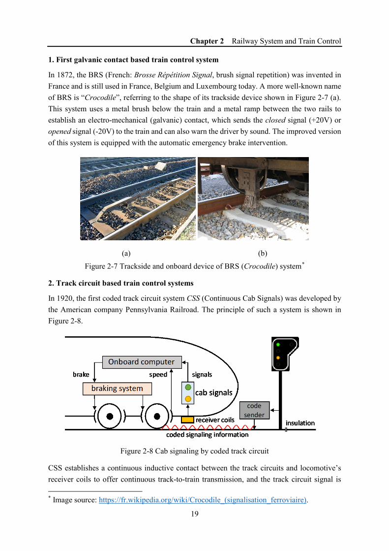
Chapter 2 Railway System and Train Control
19
1. First galvanic contact based train control system
In 1872, the BRS (French: Brosse Répétition Signal, brush signal repetition) was invented in France and is still used in France, Belgium and Luxembourg today. A more well-known name of BRS is “Crocodile”, referring to the shape of its trackside device shown in Figure 2-7 (a). This system uses a metal brush below the train and a metal ramp between the two rails to establish an electro-mechanical (galvanic) contact, which sends the closed signal (+20V) or opened signal (-20V) to the train and can also warn the driver by sound. The improved version of this system is equipped with the automatic emergency brake intervention.
(a) (b) Figure 2-7 Trackside and onboard device of BRS (Crocodile) system*
2. Track circuit based train control systems
In 1920, the first coded track circuit system CSS (Continuous Cab Signals) was developed by the American company Pennsylvania Railroad. The principle of such a system is shown in Figure 2-8.
Figure 2-8 Cab signaling by coded track circuit
CSS establishes a continuous inductive contact between the track circuits and locomotive’s receiver coils to offer continuous track-to-train transmission, and the track circuit signal is * Image source: https://fr.wikipedia.org/wiki/Crocodile_(signalisation_ferroviaire).

Chapter 2 Railway System and Train Control
20
modulated to convey more information compared to the Crocodile system. It can thus display the aspect of the next signal to the driver using colored lights in the cab. CSS is so successful a cab signaling system that some railway lines equipped CCS have given up the trackside signals to economize costs.
Meanwhile, in Europe, the idea of using track circuit to send cab signals was also applied in many countries, such as BACC in Italy, EVM in Hungary, ATB in the Netherlands, ALSN in Russia.
In France, TVM (French: Transmission Voie-Machine, track-to-train transmission) is a successful track circuit based train control system deployed in France for TGV (French: Train à Grande Vitesse, high-speed train) lines. TVM is based on the track circuit systems UM71 (analog track circuit for TVM300) / UM2000 (digital track circuit for TVM430). TVM is also used in the Channel Tunnel between France and the UK, the High Speed 1 (HS1, legally the Channel Tunnel Rail Link, CTRL) in the UK and the High-Speed Line 1 (HSL 1) in Belgium.
3. Spot inductive contact or balise-based train control systems
In 1931, the German company Siemens developed a spot inductive train control system PZB (German: Punktförmige Zugbeeinflussung, point-shaped train control), with its former name INDUSI (short for “Induktive Zugsicherung” in German, which means "inductive train protection"). The train control information is delivered by an inductive contact in discrete spots from the trackside resonator (transponder) installed at appropriate locations to the onboard generator (reader), as shown in Figure 2-9.
(a) (b) Figure 2-9 Transponder and reader in PZB*
In the same period and based on similar ideas, Switzerland started to introduce its magnet-based Signum system since 1933. Nowadays, the similar spot inductive contact is used in many sophisticated control train control systems as a complementarity to the track circuit transmission. The trackside transponder is called “balise” and has been introduced in §2.2.3.3.
* Image sources: (a) https://en.wikipedia.org/wiki/Punktf%C3%B6rmige_Zugbeeinflussung; (b) https://commons.wikimedia.org/wiki/File:Indusi_TRAXX.JPG.

Chapter 2 Railway System and Train Control
21
The train control systems using balise include the KVB (in France), the ZUB, the Ebicab, etc. Balise is also used for train localization purpose in the European Train Control System (ETCS). A balise which complies with the ETCS specification is called a d.
4. Continuous bi-directional communication based train control systems
Since the 1960s, train control system manufacturers started to test continuous and bi-directional communication technology in order to meet more sophisticated train control requirements.
In 1965, LZB (German: Linienzugbeeinflussung, linear train influencing) was first demonstrated in Germany. LZB uses conductor cable loops between rails and is installed in high-speed railway networks in Germany and Spain. The cable loops allow continuous and bi-directional transmission between the trackside LZB control center and the trains. However, from a modern point of view, the installation of cable loops has greatly increased the complexity of trackside equipment and thus augments the construction and maintenance cost. It is also very difficult to achieve interoperability with other train control systems.
Today, with the development of wireless communication, especially the GSM (Global System for Mobile), modern train control systems can establish a radio link between the trackside control center and the onboard equipment. The wireless communication is continuous, bi-directional and has a big advantage in communication capacity and compatibility.
Some examples of radio-based train control systems are: FZB and FFB in Germany, ETCS (level 2 and level 3) in Europe, ATACS in Japan, and CTCS (level 3) in China.
In 2017, there are nearly 30 different signaling systems in Europe (European Commission 2017a), and we have shown the major systems on a map in Figure 2-10.
Figure 2-10 Major national signaling systems in Europe (in 2017)
Ebicab 700 / L 10000
Ebicab 900
ZUB 123
PZB / LZB / FZB
SHP / KHP
EVM
PZB / LZB
AWS / TPWS
BRS / TBL / TVM
TVM / KVB
ASFA / LZB
Ebicab 700
Signum / ZUB 121
BACC / RSDD
ATB
LS + AVV

Chapter 2 Railway System and Train Control
22
2.4 Automatic Train Control (ATC) of Metro Systems and CBTC
2.4.1 Metro Systems and Grades of Automation (GoA)
Compared to the mainline railway network, a metro (subway) system is quite different and is often less complex due to the following reasons:
- Most metro lines are double-track systems and have barely junction or crossing between lines (there may have “junction” stations in the urban metro network composed by multiple metro lines, but normally they are not physical rail junctions);
- The rolling stock (all the vehicles) in a metro line is homogeneous;
- The speed of a metro train is relatively low (normally less than 80km/h);
- The environment of a metro system is an enclosed space, without level crossing, which can prevent the presence of a person or an obstacle on the rails.
These conveniences have given metro systems the chance of being a pioneer to apply higher-level automated technologies prior to the mainline railway network.
With the development of automated metro systems, several different Grades of Automation (GoA) for metro and railway systems are defined in IEC 62267/62290 standards (IEC 2009; IEC 2014), as shown in Table 2-1.
Table 2-1 Grades of Automation (GoA)
GoA Description Speed supervision
Acceleration and braking
Obstacle detection
Door closing
Emergency situations
GoA0 On-sight Driver Driver Driver Driver Driver
GoA1 Non-automated Partial Driver Driver Driver Driver
GoA2 Semi-Automated Auto Auto Driver Driver Driver
GoA3 Driverless Auto Auto Auto Partial Driver
GoA4 Unattended Auto Auto Auto Auto Auto

Chapter 2 Railway System and Train Control
23
2.4.2 Automatic Train Control (ATC) System
An Automatic Train Control (ATC) system can be used to control the modern metro systems. It usually has the following three functions: Automatic Train Protection (ATP), Automatic Train Operation (ATO) and Automatic Train Supervision (ATS).
Automatic Train Protection (ATP) is responsible to avoid collisions with another train. ATP ensures that the speed of a train is compatible with the authorized speed. If necessary, ATP automatically executes an emergency brake to stop the train. A train control system equipped with ATP corresponds (at least) to GoA1, which is also the most common situation of train control systems for current mainline railway networks, e.g., the ERTMS/ETCS system (c.f., §2.6)
Automatic Train Operation (ATO) implements partial or complete automatic train piloting (acceleration and braking) and performs the functions of a driver. A system can be called ATO when it corresponds (at least) to GoA2. Recent systems may implement a completely automated control system and are thus “driverless” (GoA3), nevertheless in most cases a driver is always onboard to mitigate risks of emergency situations or unintended failures.
Automatic Train Supervision (ATS) allows the supervision in the trackside control and operation center to display train status. ATS may also perform remote control for individual trains. ATS can thus be used to adjust the train’s performance to optimize its schedules, to minimize the inconveniences caused by irregularities, or to perform any other remote action based on staff’s intervention.
It is worth noting the confusing usage of some “ATx” terminologies. In this section and in the context of metro systems, these terms refer to a kind of train control systems or a general function. However, they are also names of some specific train control systems. For example, the term “ATC” in (Matsumoto et al. 2001) refers to a Japanese train control system family used for high-speed trains as a replacement for its predecessor “ATS” (Automatic Train Stop, another Japanese train control system). In the UK, “ATC” (Vincze and Tarnai 2006) is also the name of an earlier Crocodile-like British train control system installed on the Great Western Railway since 1906 and has been gradually supplanted by AWS.
2.4.3 Communications-Based Train Control (CBTC)
The automation of train control for metro systems is also driven by the development of Communications-Based Train Control (CBTC) technology.
As defined in the IEEE 1474 standard (IEEE Std. 2004), a CBTC system is a continuous, automatic train control system with the following features:
- High-resolution train location determination techniques which are independent of track circuits;

Chapter 2 Railway System and Train Control
24
- Continuous, high-capacity, bi-directional train-to-trackside data communications;
- The onboard and trackside equipment implement ATP functions, as well as optional ATO and ATS functions.
In practice, the CBTC systems are developed by different companies and vary a lot in scope, size, composition and use different concrete technologies to implement the abstract international standards. Some CBTC systems and the corresponding standards can be found in (Ferrari et al. 2012). Nowadays there have been lots of examples of CBTC systems all around the world, including Paris Métro (Line 1, 3, 5 and 13), Barcelona Metro (Line 9 and 11), Beijing Subway (Line 1, 4, 2, 6, 8, 9, 10, 15, Daxing Line, Fangshan Line and Airport Express) and several lines in New York City Subway.
Besides the high automation degree, the major CBTC systems usually have the following two features: moving block and radio-based communication.
Moving block
Unlike traditional track circuit based railway control systems where the blocks are always fixed, a CBTC system can use the moving block concept thanks to its modern positioning technology. The moving block is also defined in ETCS level 3 and more details have been introduced in §2.5.
A CBTC system based on moving block captures a train's exact position via continuous communication and uses the target-distance curve to control the train speed. It can thus adopt a higher-level flexibility and more accurate control mechanism to guarantee the safe distance between adjacent trains while improving the efficiency.
Radio-based communication
In history, CBTC has its former origins in the inductive loop based systems developed by Alcatel SEL (now Thales) for the Bombardier Automated Rapid Transit (ART) systems in Canada during the mid-1980s, which were also referred to as Transmission-Based Train Control (TBTC). AirTrain for San Francisco International Airport (SFO) was the first radio-based CBTC system and nowadays most CBTC systems use radio-based communication technologies, such as leaky coaxial cables (Wang et al. 2016), leaky waveguide (Heddebaut 2009), Wi-Fi (Zhu et al. 2009), GSM and LTE (Choi et al. 2015).
The update to CBTC systems is economically effective for stakeholders. A report by the Federal Transit Administration (FTA) in the US has shown that the application of a moving block CBTC is much better than a traditional three-speed code fixed-block train control in safety, reliability, capacity, system diagnostics, and operational cost (Rojas and Phillips 2011).

Chapter 2 Railway System and Train Control
25
2.5 Development Tendency of Train Control Systems
The history of the of train control systems has shown some tendencies in the following categories, which may also be used to infer the upcoming features of future systems.
2.5.1 Information transmission
In order to increase the speed, to reduce the safety distance and to optimize the capacity, there are several tendencies in the development of train control systems:
- from discrete (spotted) transmission to continuous transmission;
- from one-way (trackside to onboard) information chain to bi-directional information exchange;
- from analog signals to digital signals.
Several modern communication techniques with the above features, e.g., GSM, Wi-Fi, leaky waveguide, loop cables, have been used in the recent train control systems. It is worth noting that more and more train control systems have chosen the GSM-based technology since it is well-developed and low-cost.
2.5.2 Onboard and trackside equipment
From a structural point of view, another tendency of train control system development is the modularization and intelligentization of onboard equipment along with the diminution of trackside infrastructure. Owing to some historical reasons, old train control systems depend much on different trackside devices to complete train detection, localization, speed control, automatic braking, etc. These trackside systems, potentially invented in different historical periods, require a long construction cycle with high cost, only work with limited compatible onboard systems, and are difficult to be updated. Therefore, modern train control systems assign more and more roles and tasks to onboard equipment and use modular and intelligent onboard devices to save cost and to achieve better interoperability. For example, instead of receiving braking curve from the trackside (e.g., LZB), modern onboard equipment can perform the real-time calculation of a target-distance speed curve (e.g., ETCS level-2/3). The one-step braking operation can be applied by considering the target-distance speed curve and the braking performance of each train, which finally reduces the braking distance.
2.5.3 Moving blocks
In order to increase the railway network capacity, the interval distance between two trains should be reduced. In a traditional fixed block railway line (presented in §2.2.3), the interval distance is related to the train speed as well as the block partition. However, the fixed block

Chapter 2 Railway System and Train Control
26
length is calculated by the most rigorous case (high speed and poor braking performance), which will no doubt affect the capacity of the whole railway line of mixed types of trains.
Different from the fixed block sections defined by track circuit insulation, a moving block system does not have physical blocks. Safe zones around each train are calculated by computers in real time, as shown in Figure 2-11.
Figure 2-11 Moving block system
A moving block system requires continuous and bi-directional communication between the trackside and the trains to know the real-time location and speed of each train. Moving block allows reducing interval distance between trains while maintaining the necessary safety distance, which can thereby increase the overall capacity of the railway network.
Moving block is considered in ERTMS/ ETCS level 3, which is not yet implemented in Europe. Whereas the concept of moving block has been applied in the Japanese ATACS and some metro systems using Communications-Based Train Control (CBTC).
2.5.4 Interoperability and fusion of different train control systems
Figure 2-10 has shown the diversity of train control systems. Normally these systems are incompatible with each other, which causes the interoperability problem for international trains and even for domestic trains operated across the railway lines equipped with different train control systems. In Europe, the unique solution for interoperability is ERTMS/ETCS, which takes advantage of different train control systems and defines several operation levels for different applications. ERTMS/ETCS is expected to replace many national train control systems in the various member states of the European Union.
Since more and more study and application of ETCS, there have appeared several ETCS-like train control systems (or those can be referred to certain ETCS levels), such as the Chinese Train Control System (CTCS). There are also some studies about a new Unified Train Control System – UTCS (Nakamura 2016).
fixed block
Operation Direction
occupancy
fixed block
occupancy
exact positionexact position
(a) Fixed block system
(b) Moving block system
Braking curve
Braking curve

Chapter 2 Railway System and Train Control
27
From the technical point of view, we also see a tendency of the fusion of train control for mainline railway networks and those for metro systems, with the help of the development of CBTC. Metro systems have efficiently utilized the advantages of the mature technology developed by the train control systems for the mainline railway network, and can be a pioneer to test the latest techniques such as moving block, driverless train operation, etc. On the other hand, the mainline railway operators have also announced to develop autonomous trains (Bahn 2017; SNCF 2017), which is certainly motivated by the successful application in automated metro systems. The concept “ATO over ETCS” is proposed (Emery 2017) to integrate Automatic Train Operation (ATO) function in the existing ERTMS/ETCS system for mainline railway network. A Next Generation Train Control (NGTC) project has also been proposed to develop a uniform train control system for both mainline and urban networks, benefiting from the advantages of both the ETCS and CBTC.
2.6 ERTMS / ETCS
2.6.1 Necessity of Developing and implementing ERTMS
The interoperability problem of different train control systems is particularly outstanding in Europe since many European countries close to each other, where the international railway lines are very common. Thanks to the European Union and the Schengen Agreement, it is usually not necessary for international trains to stop at borders for border inspection from the governmental point of view.
However, even though the railway networks are well developed in European countries, especially in Western and Central Europe, these countries have their own national train control systems as shown in Figure 2-10, which causes the famous interoperability problem for international trains. Currently, there are two solutions for international trains to pass the borders in Europe:
(1) The cab should be equipped with different train control systems onboard, and the handover process usually requires a stop or a slowing-down.
(2) The train should stop at the border and the locomotive should be changed to a national one (the driver may also be changed).
The first solution leads to a very complex configuration of the onboard system for international trains, which increases the installation and maintenance costs; while the second solution is quite time-consuming and thus arises a conflict with the optimization and efficiency requirements by the railway stakeholders. In this context, the idea of developing a unified European railway control system was born since more than 20 years ago.
ERTMS (the European Railway Traffic Management System) is a solution for the interoperability of trains in European railway network. It aims to develop a complete,

Chapter 2 Railway System and Train Control
28
interoperable, modular and generic system of railway control and management shared by all European national operators. In addition to the interoperability, which is obviously the main benefit, ERTMS increases the railway network capacity as well as guarantees a higher level of safety, reliability, punctuality, and cost-effectiveness, compared to a majority of the existing national signaling systems.
Nowadays, ERTMS has been agreed as the unique railway signaling system in Europe by all the Member States. The development of ERTMS is part of the European harmonization process and the implementation of ERTMS is assured by European Union law (European Commission 2017b). The migration process from different national train control systems to a unique ERTMS is a huge challenge but is already in progress.
2.6.2 ERTMS Specifications and Legislation
The ERTMS-related specifications and legislation can be classified into three levels:
1) High-level essential requirements;
2) Legal description of ERTMS main functions, components, and subsystems;
3) Complete technical specifications to achieve interoperability e.g. system requirements, functional interface specifications, dimensioning rules, performance…
From a hierarchical point of view, the highest-level document related to the interoperability for the European railway network is the Interoperability Directive (2008/57/EC) (European Commission 2008). This EC Directive is currently in force, setting out the interoperability requirements about safety, reliability, availability, health, environmental protection and compatibility with other subsystems. The EC recommendation (2014/897/EC) (European Commission 2014) has defined the procedure to put ERTMS into service.
A legal description of ERTMS specification is the Technical Specifications of Interoperability for Control Command and Signaling (TSI CCS) (European Commission 2016). From the legal point of view, this EU regulation should be applied directly to all member states without a transposition to the national law. It defines the essential ERTMS requirements, the functional and technical specifications of subsystems and interfaces, as well as the necessary methods and procedures for system assessment.
The complete technical specifications can be found in Annex A of the CCS TSI (European Union Agency for Railways 2016), which defines a list of several “subsets” of the ERTMS system requirements specification and functional description of its different constituents, among which there are two types of documents:
• Mandatory specifications, which must be fulfilled by all ERTMS systems, subsystems or components to achieve the interoperability. Any deviation from the mandatory
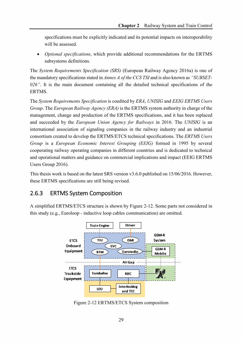
Chapter 2 Railway System and Train Control
29
specifications must be explicitly indicated and its potential impacts on interoperability will be assessed.
• Optional specifications, which provide additional recommendations for the ERTMS subsystems definitions.
The System Requirements Specification (SRS) (European Railway Agency 2016a) is one of the mandatory specifications stated in Annex A of the CCS TSI and is also known as “SUBSET-026”. It is the main document containing all the detailed technical specifications of the ERTMS.
The System Requirements Specification is coedited by ERA, UNISIG and EEIG ERTMS Users Group. The European Railway Agency (ERA) is the ERTMS system authority in charge of the management, change and production of the ERTMS specifications, and it has been replaced and succeeded by the European Union Agency for Railways in 2016. The UNISIG is an international association of signaling companies in the railway industry and an industrial consortium created to develop the ERTMS/ETCS technical specifications. The ERTMS Users Group is a European Economic Interest Grouping (EEIG) formed in 1995 by several cooperating railway operating companies in different countries and is dedicated to technical and operational matters and guidance on commercial implications and impact (EEIG ERTMS Users Group 2016).
This thesis work is based on the latest SRS version v3.6.0 published on 15/06/2016. However, these ERTMS specifications are still being revised.
2.6.3 ERTMS System Composition
A simplified ERTMS/ETCS structure is shown by Figure 2-12. Some parts not considered in this study (e.g., Euroloop - inductive loop cables communication) are omitted.
Figure 2-12 ERTMS/ETCS System composition
Chapter 2 Railway System and Train Control
30
ERTMS is globally composed of two main parts:
- ETCS, the European Train Control System, shown by the blue parts in Figure 2-12;
- GSM-R (Global System for Mobile Communications – Railways), a GSM-based radio system providing voice and data communications between the trackside and trains, as shown by the green part in Figure 2-12.
ETCS can be further divided into ETCS onboard system and ETCS trackside system.
Onboard Equipment
ETCS onboard system interacts with a driver by using a normalized interface DMI (Display Machine Interface) and can control the train engine and the braking system via TIU (Train Interface Unit). Each train is equipped with one or more GSM-R mobiles which support the Euroradio protocol. The ATP (Automatic Train Protection) functions such as braking curve calculation are processed in EVC (European Vital Computer), which will be further introduced in §2.6.4 based on different ETCS levels.
Trackside Equipment
The most important trackside devices are RBC (Radio Block Centre) and Eurobalise. These two devices are also connected to other trackside signaling systems beyond the ERTMS/ETCS scope (shown as the yellow part in Figure 2-12), such as interlocking system and Traffic Control Center (TCC).
An RBC manages the trains in a defined area to ensure the safe distance between the neighboring trains. Bi-directional continuous communication between the trains and the RBC via GSM-R (for ETCS level 2 or level 3) is established. When a train crosses the border of two areas managed by different RBCs, it needs a specific operation “RBC handover”.
A Eurobalise is a specific type of balise used in ETCS. Eurobalises are mainly used for localization purpose and can offer position telegrams to the trains passing over them. Whereas some transparent data balises can pick up signal aspects from the existing trackside signals via LEU (Lineside Electronics Unit (LEU) and send them to the trains to realize the cab signaling. Trackside data can also be sent to trains in this way. The balise telegrams are received by onboard equipment via BTM (Balise Transmission Module).
2.6.4 ETCS Levels and their Train Control Methods
ERTMS/ETCS is specified in several different application levels (levels for short hereinafter) to achieve the possible operating compatibilities between trackside and trains. Different levels require different installations of the trackside/onboard equipment and can support different train control functions.

Chapter 2 Railway System and Train Control
31
In the latest ERTMS/ETCS System Requirements Specification Baseline 3 (European Railway Agency 2016a), five levels are defined: level 0, level NTC, level 1, level 2 and level 3. Levels are downwards compatible for ETCS onboard system, for example, an ETCS-2 equipped train can also operate on ETCS-1 equipped lines.
Level 0
Level 0 is defined for non-ETCS trackside condition. It applies when an ETCS-equipped train operates on a non-ETCS railway line.
Level NTC
Level NTC (National Train Control) is newly defined in ERTMS/ETCS Baseline 3 and replaces the former name STM (Specific Transmission Modules). It is in fact a compromise for the interoperability of a railway line already equipped with a well-developed national system (e.g., in France and Germany).
Level 1
Level 1 is for the ETCS-equipped trains to operate on a railway line equipped with Eurobalises but without RBC and GSM-R. In practice, Level 1 is usually superimposed over an existing signaling system. In level 1, Eurobalises pick up signal aspects from the existing signaling system and transmit Movement Authority (MA, permission for a train to move to a specific location with the supervision of speed) to trains at discrete spots. The onboard computer EVC calculates the braking curve and continuously monitors the speed.
Due to the spot transmission method, a train must travel over a Eurobalise to obtain or update its MA. Hence, when a train is at a standstill, it needs another way (e.g., physical trackside signals) to get the first permission to start its travel. Some infill techniques (Euroloop or radio or extra balises) are defined to improve the performance in level 1 but are rarely applied.
Figure 2-13 ETCS level 2 schematic
braking
onboard EVC
Eurobalise
DMIpositionspeed
STM
GSM-R Mobile
RBC
MA
position reports
Interlocking
track circuit
TCC
ETCS-2 line
ETCS Equipped Eurocab

Chapter 2 Railway System and Train Control
32
Level 2
Level 2 is used for a railway line controlled by Radio Block Centre (RBC) and equipped with Eurobalises and Euroradio. It is based on bi-directional continuous data communications between RBC and trains via GSM-R.
As shown in Figure 2-13, level 2 has the following features:
- No more physical trackside signals required;
- Eurobalises are only used for location reference purpose. Between the Eurobalises, the train can continuously determine its exact position (e.g., by counting wheel rotations). It can report its current position to RBC via GSM-R at any time when necessary;
- Movement authorities (MA) can be continuously transmitted from RBC to each train through GSM-R, together with authorized speed and route data (slopes, curves, etc.). RBC is responsible for MA generation as it knows from trains their positions and collects the information from other trackside systems such as the track circuits, interlocking system and TCC.
- Onboard EVC calculates a speed profile taking into account the received MA and the train’s characteristics (mass, length, braking performance, etc.). The authorized speed is continuously displayed to the driver and is also monitored by ATP to apply braking in case of a speed excess.
- Train detection and train integrity check are performed by trackside equipment.
ETCS Level 2 is a successful application level as it combines many advantages:
- Long-term compatibility with many existing national railway lines in Europe is guaranteed by the use of Eurobalises;
- Reliable continuous bi-directional trackside - train transmission ensured by the low-cost and mature radio communication technology GSM-R;
- The possibility to abandon the trackside signals can minimize trackside equipment, which reduces time and costs for infrastructure implementation and maintenance.
Currently, ETCS level 2 is the most interesting level being applied in Europe and studied around the world. For this reason, we have chosen level 2 as our major research subject.
Level 3
It is based on the train control methods of level 2, with the following differences:
- Train integrity check is performed by onboard equipment (vs. by trackside in level 2); - Moving block is applied for track occupation check, track circuit is therefore not
necessary (track circuit may be still used at specific locations, e.g., shunting).
Level 3 is still a future standard that has not yet been implemented.

Chapter 2 Railway System and Train Control
33
Level transitions
Level transitions are an important function in ERTMS/ETCS. For example, a train coming from level 1 area and entering to level 2 area needs to operate a special procedure for the level transition. Before the level transition, some conditions need to be satisfied, e.g., the registration to the GSM-R network, the establishment of the communication with RBC, the MA and the system configuration parameters received from RBC. With all the conditions satisfied, the train will operate the transition level 1 to level 2 at a level transition point.
2.7 Conclusion of Chapter 2
This chapter introduces the railway systems and train control systems.
Some basic concepts in railway system are presented to help the reader better understand our research work.
We introduce the railway control systems in three sections, emphasizing their application in mainline railway networks, in automated metro systems, and their development trends, respectively.
The objective of the study of train control systems is to build intelligent rail infrastructure, intelligent mobility management, smart rail services, and a new generation of railway vehicles ultimately form the requirements of a seamless high data rate wireless connectivity for future rail development, as specified in the European “Shift2Rail” project*.
At the end of this section, we are interested in ERTMS/ETCS because it is currently one of the best train control systems and is widely used not only in Europe but around the world.
The ETCS level 2 is chosen as the target system to support the rest of this study as it can be regarded as a good example of complex discrete event systems (DES). It is also a safety-critical system and thus needs to be modeled and validated by appropriate methods, which is the objective of this thesis.
* http://www.shift2rail.org/


35
Chapter 3 STATE-OF-THE-ART FOR THE TRAIN CONTROL SYSTEM DEVELOPMENT
3.1 Introduction to Chapter 3
This chapter is the literature review of different approaches to study the development of train control systems, an example of complex discrete event systems (DES).
§3.2 considers all the phases in the system development life cycle of the train control systems and introduces various methods applicable for each phase. By introducing and comparing a large number of approaches we justify our choice of Petri nets as the modeling formalism.
§3.3 concentrates on Petri nets as this formalism has been chosen to model the train control systems in this study. Different Petri net variants are discussed, where two high-level Petri nets variants – colored Petri nets (CPN) and well-formed Petri nets (WFN) – are underlined. For the readers not familiar to Petri nets, the introduction to Petri nets offered in Appendix A should be helpful to approach to the topic.
§3.4 presents some related research about the Petri nets based modeling methods and will be focused on CPN and WFN. The discussion and comparison of these two formalisms are also given to balance the efficient modeling expressivity and the potential to facilitate the verification phase.
§3.5 conclude this chapter.
3.2 Review of Methods for Train Control Systems
Development
3.2.1 Railway Safety Standards and Formal Methods
3.2.1.1 Railway safety standards
With the increasing complexity and degree of automation of transportation systems, the development of such a system with guarantee becomes more and more difficult. It also gives high priority to the system development methods that ensure the safety. In this context, several safety-related standards have been created for different application domains, as shown in Figure 3-1.

Chapter 3 State-of-the-Art for the Train Control System Development
36
Figure 3-1 Safety related standards
Among these standards, IEC 61508 is of our particular interest as it serves as the basis for some domain-specific standards, e.g., railway systems.
In Europe, the European Committee for Electrotechnical Standardization (CENELEC) applies IEC 61508 to different domains by creating several European standards. The following standards (CENELEC 2003; CENELEC 2010; CENELEC 2011; CENELEC 2017) are used as a mandatory for system design and application in the railway industry.
• EN 50126:2017—The specification and demonstration of Reliability, Availability, Maintainability, and Safety (RAMS)
• EN 50128:2011—Software for railway control and protection systems.
• EN 50129:2003—Safety-related electronic systems for signaling.
• EN 50159:2010—Safety-related communication in transmission systems.
Table 3-1 Safety Integrity Levels (SIL) Definition
SIL Demand Mode*:
probability of failure on demand (PFD) Continuous Mode:
probability of failure per hour (PFH)
SIL-4 10−5 ≤ PFD < 10−4 10−9 ≤ PF < 10−8
SIL-3 10−4 ≤ PFD < 10−3 10−8 ≤ PF < 10−7
SIL-2 10−3 ≤ PFD < 10−2 10−7 ≤ PF < 10−6
SIL-1 10−2 ≤ PFD < 10−1 10−6 ≤ PF < 10−5
SIL-0 Safety systems not required to meet a SIL standard are referred to as SIL-0.
* “Demand Mode” is defined in IEC 61508 but is abandoned in EN 50129.

Chapter 3 State-of-the-Art for the Train Control System Development
37
In these safety-related standards, five Safety Integrity Levels (SIL) from SIL-0 (lowest level) to SIL-4 (highest level) are defined, as shown in Table 3-1.
These safety standards are used as a framework to guide and to estimate the system safety. In order to provide concrete and appropriate methods and techniques for the systems development, formal methods are strongly recommended in these safety-related standards to be applied throughout all the phases of the system development (Boulanger 2014).
3.2.1.2 Formal methods application in the railway industry
Formal methods are a particular kind of techniques based on mathematics and logical reasoning for the specification, design, and verification of software and hardware systems. There are a large number of formal methods, and they share some advantages:
- Formal representations have precise semantics which is free of ambiguity;
- Formal models can be mathematically verified and are thus proved to be correct;
- Formal models can be read by computers, which allows the automated or semi-automated development process.
In fact, the railway industry is always regarded as a leader in the adoption of formal methods. IEC 61508 “highly recommended” formal methods for SIL-4 systems and functions. In the railway industry domain, EN 50128 “recommends” formal methods for SIL-1/2 systems, and “highly recommends” them for SIL-3/4 systems in the following modeling phases:
• Software Requirements Specification (Table A.2 in (CENELEC 2011))
• Software Architecture (Table A.3 in (CENELEC 2011))
• Modeling (Table A.17 in (CENELEC 2011))
Also in the verification and testing phase, formal proof is “recommended” for SIL-1/2 and “highly recommended” for SIL-3/4 (Table A.5 in (CENELEC 2011)). Formal proof of correctness of data is “highly recommended” for SIL-3/4 to be used as data preparation techniques (Table A.5 in (CENELEC 2011)).
Some concrete formal methods, e.g., Timed Petri Nets, are also recommended in EN 50128.
This study will only concentrate on formal methods in the DES development. It is worth noting that formal methods can also be used in continuous systems or hybrid systems. For example, Sandia National Laboratories (Department of Energy, USA) has conducted some research based on the Bay Area Rapid Transit (BART) to design and validate the train acceleration control function with continuous profiles (Kapur et al. 2001); the German Transregional Collaborative Research Center - AVACS (Automatic Verification and Analysis of Complex System) has also studied formal verification by taking the ETCS as an example of hybrid system (Platzer and Quesel 2009).

Chapter 3 State-of-the-Art for the Train Control System Development
38
Different formalisms appropriate for train control system development (a majority of which are formal methods) are presented in Figure 3-2 to give the readers a general idea. This figure also shows the major application phase of each method in a whole development lifecycle. However, please note that many methods are not dedicated to just one phase.
Figure 3-2 Methods and tools for train control system development
In the following sections of §3.2, different formalisms used in the train control system development will be introduced:
• §3.2.2 introduces the modeling, verification and validation methods in the system requirements specification phase;
• §3.2.3 and §3.2.4 present the modeling methods in the system design modeling phase and the implementation phase, respectively;
• §3.2.5 introduces the verification and validation techniques used in system design modeling phase and implementation phase;
• §3.2.6 presents some tools that can be used in the whole lifecycle development for train control systems.
3.2.2 Requirements Specification Methods
In the very early stage of the development of train control systems, it is necessary to collect the system requirements.
A requirement specifies the capability (which may be performed by a function) the system should satisfy or the performance condition that the system must achieve (Belloir et al. 2014).
Once the system requirements are defined, the specification documents are obtained.
System requirements specifications are usually written in natural languages (e.g., English, French) as it is the most intuitive way for engineering applications. These specification
Whole Lifecycle Development Tools (Rodin, SCADE, CPN Tools)
Requirement specification phase
UML, SysML,PSL; SDL; SCP,Z notation, B
Method, VDM
Manual inspection;Simulation;
Test;Formal
Verification
System design phase
Petri Nets, Automata,
UPPAAL, Raise, AADL
Model Checking;Theorem proving;
Computer Simulation
Implementation phase
SFC,VHDL, C, C++
Simulation Platform;Test Case
Generation
IBM Rational Software, RATSY
ProB, CASDL Tester, PHAVer,
Atelier B
CPN Tools, TINA, DESUMA, Supremica
NuSMV, PRISM, PVS,
UPPAAL-SMC (for simulation)
Unity PRO (Schneider),
Step 7 (Siemens)
HIL, RailSim, OpenTrack;
For Test: Holodesk
System development
life cycle
Examples of Tools and platforms
Examples of formalism
Modeling Verification Modeling Verification Implementation Verification

Chapter 3 State-of-the-Art for the Train Control System Development
39
documents are then served as the basis for the following system design and implementation stages.
Even though these specification documents in natural languages can be inspected by domain experts against the potential errors, there is no deterministic assurance by such a manual inspection. Obviously, these documents are also difficult to be validated or to be integrated into the development lifecycle in an automated way.
In order to guarantee the correctness and the conformity within the specification, formal methods are strongly recommended for the system specifications. Two stages starting from the specification documents are usually necessary:
• Specification modeling according to the specification documents;
• Specification verification on the undertaken models.
3.2.2.1 Requirement Modeling Methods and Tools
Among the numerous formal methods created with different characteristics and special applicability, a lot of them can be used to model specifications. While, very few of them have been proven to be adapted for modeling railway system specifications.
These methods include Z notation, B-Method, the Vienna Development Method (VDM), OBJ, etc. These methods adapted for railway specifications can be classified by several groups:
Logic-based methods and especially the B method
There is a large set of formal methods based on the set theory and first-order logic. These methods are usually used for requirements specification modeling by rewriting the specifications using well-defined syntax which has mathematically precise semantics. Then, verification and analysis can be done on the specification models by using logical deduction reasoning and/or theorem proving methods. A theorem proving process can be manual or interactive or automated (thus called automated theorem proving in this case).
On the other hand, by an iteration process of the system refinement, some logic-based methods can finally generate the refined models which facilitate the following system design and implementation phase.
The first use of formal methods in the French railway industry can be dated to the beginning of 1980 with the Vital Coded Processor (VCP) technique for the SACEM project, an automatic train control system demanded by RATP (French: Régie Autonome des Transports Parisiens, Autonomous Operator of Parisian Transports). Later in 1992, B method was chosen by Siemens Mobility (known as “Matra Transport International” before 2001) to develop and validate the automatic train operation system for Paris Metro Line 14 (known as “Météor” project in history) in order to prevent software design errors and to reach zero-fault (Behm et al. 1999). During the system development using the B method, 27,800 lemmas had been

Chapter 3 State-of-the-Art for the Train Control System Development
40
proven, 90% of which were proven automatically, and the rest were proven interactively. Many errors were found during the proving activities while no further bugs were detected in the testing phase after that. It is thus considered as a good example of formal method application and has also made B method popular in the development of railway system requirements specification in France and in Europe.
B method was invented by Jean-Raymond Abrial (Abrial 2005). It describes a system as an Abstract Machine, which includes a set of states and a set of operations that modify the state values. An invariant predicate is defined on each state; a pre-condition and a post-condition are defined on each operation to describe the effect(s) of the operation on state values. When executing an operation in a state, it must be proved that both the pre-condition of operation and the invariant predicate are satisfied, and the state after the execution satisfies both the post-condition and the invariant predicate. When it comes to the refinement, it must be proved that the required system properties are preserved. Thus, a specification is transformed into a set of proof obligations, which can be later verified in the theorem provers.
The successor of B method is Event-B (Abrial 2010) which was later invented by the same author Abrial with the extension of event support. Today, B method and Event-B are both widely used in the requirements specification engineering of modern train control system. In (Abo and Voisin 2013), B method is used to model the data validation process in the trackside system of CBTC, as a result, some mistakes in the requirements specification are found and corrected; in (Reichl et al. 2016), Event-B model is used for the verification and validation of a railway interlocking system.
Other similar formal methods usually used in the railway industry include VDM (Vienna Development Method), Z notation and OBJ, which are invented before the B method.
In (Hansen 1994), VDM is used to model and validate the principles and concepts of the Danish railway interlocking systems together with the simulation by ML.
Besides the requirements specification modeling, Z notation is also able to model the data and operations. In (Faber et al. 2007), Z notation is used to model the complex data types defined in the requirements specification and to describe the Radio Block Centre (RBC) in ETCS.
A study based on the railway interlocking system specification models and validates the moving block concept using both Z notation (Zafar 2009; Zafar et al. 2012) and VDM (Zafar 2006).
Process calculus based methods
Process calculus based formal methods pays attention to concurrent behaviors and are appropriate for modeling the interactions between different components or simultaneous processes.

Chapter 3 State-of-the-Art for the Train Control System Development
41
CSP (Hoare 1978) was invented by Hoare in 1978 for distributed and concurrent software design. It can be used in railway control domain to model and verify some results caused by concurrent processes. In (Faber et al. 2007), CSP is used to model two concurrent train control processes in ETCS: the train operation control and the emergency message treatment.
CSP can also be used with a hybrid extension Hybrid CSP. In (Zou et al. 2013), several operational scenarios defined in the system requirements specification of Chinese Train Control System (CTCS) are modeled with Hybrid CSP to support the uncertainty analysis of the mode transitions.
Some other similar formal methods based on process calculus include: Calculus of Communicating Systems (CCS) (Milner 1980), which is useful for evaluating the qualitative correctness such as deadlock or livelock; LOTOS (ISO 1989), an ISO (International Organization for Standardization) standard of a formal description method based on the temporal order of observational behavior. The difference between these methods can be found in (Fidge 1994).
Property-based methods
A common property-based language is Property Specification Language (PSL), initially developed by Accellera as a hardware description language (HDL) to specify properties and assertions in hardware designs. PSL subsumes the linear temporal logic LTL-style (Pnueli 1977) operators with the aim of both the ease of expression and the enhancement of its expressive power.
Besides the hardware design, PSL can also be used in requirements specification in industry. The requirements specification modeled by PSL consist of:
• Formal models defining the system behaviors;
• A set of assertions defining the obligations of the system behaviors;
• A set of properties defining the allowable behaviors of the system.
The models built with PSL can be simulated directly with RATSY (Requirements Analysis Tool with Synthesis) (Bloem et al. 2010). An example could be found in (Zhao et al. 2012), where the mode transitions rules in the requirements specification of CTCS are translated into PSL models and are then verified with the requirement analysis tool RATSY.
Description based methods
A basis of description based methods is Specification and Description Language (SDL), a formal language defined by the International Telecommunication Union–Telecommunication Standardization Sector (ITU-T) as recommendation Z.100 (ITU-T 2016).

Chapter 3 State-of-the-Art for the Train Control System Development
42
SDL was initially used for telecommunication systems and was mainly designed to specify and describe the functional behavior of systems. It is able to describe the structure, behavior, and data of a system.
SDL has a Graphic Representation (SDL/GR) and a textual Phrase Representation (SDL/PR), and both of them are equivalent to the same underlying semantics. SDL/GR has an intuitive expression which supports the object-oriented and top-down developing approaches and is convenient for engineers to use, while SDL/PR can serve as the format of exchange models for the SDL modeling tools such as SDL Suite.
In (Yuan et al. 2011), functional requirements for the onboard system of CTCS is modeled by SDL with three levels:
• System level: interface definition and onboard data exchange format;
• Module level: functions, interactivities, and data flow of each module;
• Function level: implementation of the functions.
Issad has extended SDL to SDLg (Issad et al. 2014) for the modeling of complex systems architectures, and then further extended SDLg to Scola, a Scenario Oriented Language (Issad et al. 2015) to facilitate the modeling of the complex systems such as CBTC in a more natural and intuitive way similar to UML.
UML based methods
Unified Modeling Language (UML) is a general-purpose, developmental, modeling language for industrial applications. It was adopted as an ISO standard (ISO/IEC 2005) and has become the facto specification language for most software design, especially for those using the object-oriented approach.
Different from the formal methods already introduced, UML is a semi-formal method. Even though it has a well-defined syntax, some types of UML diagrams (especially some static descriptive diagrams, e.g., class diagram) have elements provided in prose and do not have an inherent, unambiguous and mathematically precise semantics. As a result, a UML model can be computer-readable, but is difficult to be computed in a deterministic way due to the lack of completely formalized semantics.
On the other hand, there exist methods that can formally interpret some UML diagrams (e.g., State Diagrams) into a formal language to model the requirements specification (Hu 2008).
Some other trials to formalize UML propose to use formal descriptions on some UML diagrams to support formal verification. In (Chiappini et al. 2010), a constraint language CNL (Controlled Natural Language), which is based on a subset of PSL and which mixes LTL, regular expressions, first-order logic, and hybrid aspects, is proposed together with a subset of UML to model the ETCS, where:

Chapter 3 State-of-the-Art for the Train Control System Development
43
• UML Sequence diagrams are used to model the interaction between the specified objects (e.g., trackside system and onboard system) in a sequential order;
• UML State Machines are used to describe the state change of the Movement Authority (MA) management.
In (Jabri et al. 2009), UML is used to model the ERTMS specifications. An automatic transformation from UML State Machines and UML Sequence diagrams into Predicate Transition Petri Net (PrT-nets, details can be found in Appendix A) is also developed with the aim of the generation of test scenarios.
The advantage of UML based methods is the versatile expressive power inherited from the diversified charts and diagrams to model the structure and behavior of a complex system. It is also worth noting that in UML, we have the ability to create a new Domain-Specific Language (DSL) thanks to the flexibility of UML. A good example is Systems Modeling Language (SysML), defined on a subset of UML 2.0 with some extensions using UML's profile mechanism to meet the requirements of systems engineering. A DSL based on UML for the train control field is possible to be proposed by applying some constraints and extensions to the standard UML.
The weakness of a UML based method is often caused by the lack of a completely formal expression. Although there exist formalization methods, the constraints to apply these methods will no doubt limit the application of UML and weaken its advantages introduced above.
Comparison of different specification design methods
Table 3-2 Comparison of requirement modeling methods and supporting tools
Methods Behavior Safety Real-time Advantages Support Tools
UML based √ × √ Graphical, intuitive Rational Rose,
Property based √ √ × Simulation support RATSY
Description based
√ × × Top-down
approach support Rational SDL
Suite
Process calculus based
√ √ √ Concurrence
support PAT
Logic based √ √ √ Refinement
support, automated theorem proving
Atelier B
Rodin (Event-B)
Legend: √ – the method has the feature × – the method does not have the feature

Chapter 3 State-of-the-Art for the Train Control System Development
44
The advantage of UML based methods is the versatile expressive power inherited from the diversified charts and diagrams to model the structure and behavior of a complex system. It is also worth noting that in UML, we have the ability to create a new Domain-Specific Language (DSL) thanks to the flexibility of UML. A good example is Systems Modeling Language (SysML), defined on a subset of UML 2.0 with some extensions using UML's profile mechanism to meet the requirements of systems engineering. A DSL based on UML for the train control field is possible to be proposed by applying some constraints and extensions to the standard UML.
The weakness of a UML based method is often caused by the lack of a completely formal expression. Although there exist formalization methods, the constraints to apply these methods will no doubt limit the application of UML and weaken its advantages introduced above.
compares the aforementioned requirements specification methods in the aspects of their supports for behavior modeling, safety feature and real-time feature. The advantages and supporting tools for each method are also listed.
3.2.2.2 Requirements Verification and Validation
Requirements specification is the basis for the following system development process. However, due to the huge size and complexity of train control systems, it is somehow inevitable to have some defect or safety risks in the system requirements specification.
In this context, the adequate verification (i.e., the fulfillment of properties such as completeness and consistency) and validation (i.e., the correspondence of the system model with the customer needs) of requirements specification is thus necessary to prevent errors from propagating into later development phases where it will be far more expensive to correct a fault derived from the requirements specification.
In the requirements specification phase, the verification techniques are used to check the correctness, consistency and completeness.
We introduce several approaches to take on the requirements specification verification.
Requirements inspection
A requirements inspection is also called a requirement review or walk-through. It is usually a meeting where the stakeholders, domain experts, and system developers are together to walk through the requirements specification, page-by-page, line-by-line, to ensure that the specification documents represent the need of every aspect and do not contain errors, depending on the their experience. For large-scale systems, there are some requirement management tools such as IBM Rational RequisitePro to facilitate the requirement organization and inspection
Chapter 3 State-of-the-Art for the Train Control System Development
45
A requirement inspection is relatively easy to conduct and thus widely applied in the industry. However, the drawback is also obvious: one cannot obtain a formal proof by this experience-based process. Even with the help of requirement management tools, the inspection process is always a human labor and cannot be automated by computer.
Model-based requirements validation
Since the requirements specification written in natural language can only be validated manually, which may contain human errors, a more reliable means of requirements validation could be to build a model of the requirements and then to verify the model using appropriate model-based techniques.
Different kinds of models are used according to the different properties to validate,
- Mental model is used in (Lee et al. 2014) to guarantee the good understanding of the stakeholders’ needs. Through this method, it is possible to result in products that better satisfy customers’ perspective.
- Prototype model is usually used in Agile Development to help the customers validate the requirements by the interactions with a prototype other than the lecture of the documents. In (Aceituna et al. 2011), a requirement validation technique, Virtual Requirements Prototype (VRP), is proposed. On the one hand, it avoids the physical prototyping which is costly and time-consuming; on the other hand, it allows stakeholders to validate the requirements through interaction with the virtual model.
- Scenario-based model is used in (Aceituna et al. 2010) to provide an interactive and systematic way to validate a requirements model. The approach transforms the requirements into three components: a set of scenario questions, a set of constraint patterns, and a set of inference constraints. A Scenario Question Query Engine (SQ2E) can query the model by executing the scenarios.
Formal requirements verification methods
Formal verification methods can be used when the requirements specification is presented using formal models. According to the different theories on which the formal methods are based, different formal verification methods are used to achieve a logical verification.
Model-Driven Engineering (MDE) based transformation is often used in the formal verification of requirements specification. On the one hand, it can realize the model transformation between certain formal models to facilitate the verification. For example, in (Olderog 2012), The requirements models of the modular language CSP-OZ-DC are transformed into Transition Constraint Systems (TCS) by using the Phase Event Automata (PEA). As the result, the Abstraction Refinement Model Checking (ARMC) tool can be put in practice to perform the automated model checking.

Chapter 3 State-of-the-Art for the Train Control System Development
46
On the other hand, MDE technology may also allow the formal verification of several properties on semi-formal models and thus bridge the gap between the semi-formal modeling and the formal verification (Liu and Tang 2011).
The formal verification techniques can avoid the ambiguity in the requirements specification, provide a complete coverage and a high-level assurance. Some formal methods can be highly automated. These features make it appropriate to use the formal verification in the in the development of safe-critical systems. However, the formal methods themselves cannot guarantee that the formal model and formal verification correctly and completely express the final users’ intention. The application of formal methods requires the experts who know well not only the formal methods and tools, but also the domain knowledge as well as the systems to be verified.
Train control systems are finally implemented in a complicated operational environment. Formal methods are powerful in verifying the requirements specification consistency but are usually less expressive to consider the uncertain factors and external events. As a result, one may meet some difficulty to verify several properties considering the system’s behavior in a complicated environment.
Another obstacle to apply the formal methods is the famous “combinatorial explosion” problem. Lots of formal verification techniques provide the formal guarantee by analyzing all the possible system states. As the railway control system is a complex and concurrency system, the system states can be quite large or even close to infinity. The combinatorial explosion encountered during the formal verification also restricts its application range.
Table 3-3 further compares the verification methods in the requirements specification phase.
3.2.3 System Design Modeling
In the very ideal conditions, we hope that the requirements specification model could be transformed into an implementation mechanism. For the moment, the MDE techniques are not able to conduct the direct model transformation from requirements specification model to an implementation method. In practice, we need to build the system design models based on the requirements specification in the system design phase. Currently, most system design models are still built manually and are thus error-prone.
In this context, it is necessary to have some appropriate methods and techniques to build and verify the system design models. In this section, we introduce some system design methods appropriate for train control systems, among which we can see that the formal methods are also widely used in the system design phase.
From an engineering point of view, the system design models can be classified into two categories:
Chapter 3 State-of-the-Art for the Train Control System Development
47
- the structural models, static models to describe the system hierarchy and composition;
- the behavior models, dynamic models to describe the behaviors of the system.
It is worth noting that this classification is not absolute. Most modern methods can support both the structural and behavior modeling formalisms to build the complex system models.
3.2.3.1 System Structural Modeling
Architecture Analysis & Design Language (AADL)
AADL is proposed by SAE International (Society of Automotive Engineers, US) as an SAE standard AS5506 (SAE 2004). It is a language to describe the architecture of the software system and the embedded, real-time, and performance-critical systems, especially in the automotive and aerospace applications.
An AADL architecture describes the properties and interfaces of two types of components:
• execution platform components: processors, buses, memory, etc.;
• application components: application and software modules.
An AADL model mainly describes how a complete system is integrated from its components. The performance-critical aspects of the whole system can thus be analyzed by the assembly of the individual components. In (Li and Zhang 2015), several AADL models are introduced for ATP, ATO, and ATS in CBTC, emphasizing the definition of some complex types.
Besides its advantages in structural modeling, AADL can also be used to model the system behaviors via AADL behavior model defined in the annex. In (Ahmad et al. 2015), AADL is used to model the behaviors of the CTCS with Movement Authority (MA) scenario.
An open-source platform OSATE (Open Source AADL Tool Environment) can be used for modeling, analysis and code generation proposes (The SEI AADL Team 2005).
UML Based structural diagrams
The class diagrams and package diagrams in UML are widely used to build structural models in system design. Class diagrams are used in architecture or hierarchy design while package diagram is used to define the entities. As a variant and an extension of UML, SysML an better describe the system structure with its Block Definition Diagram and Internal Block Diagram.
Lots of recent studies can be found about modeling CBTC system structure using UML class and package diagrams (Yang et al. 2008; Di Claudio et al. 2014).
3.2.3.2 System Behavior Modeling
In contrast to the structural models which describe the static aspects of a system, the behavior models represent how the system works and interacts.

Chapter 3 State-of-the-Art for the Train Control System Development
48
Automata-based methods
Methods based on automata theory or, more specifically, finite-state-machine (FSM) are widely used in engineering. An FSM can make a transition from one state to another in response to the current state and external inputs. For complex system modeling, some automata extensions are also used, for example:
- Hybrid Automata (Henzinger 2000) is used in (Bu et al. 2011) to model the Movement Authority (MA) management between the trains and the RBC;
- Timed Automata (Alur and Dill 1994) is used in (Khan et al. 2016) to model a computer-based automated interlocking system.
There are many modeling tools based on automata theory, where one of the most popular tools is UPPAAL (Bengtsson et al. 1995), jointly developed by Uppsala University in Sweden and Aalborg University in Denmark. UPPAAL is a modeling and verification tool based on timed automata. In (Sacha 2008), dependable train controller models are originally built by UML State Machine and then conversed to the timed finite state machine. The latter is then checked with UPPAAL and finally transformed to PLC code in STEP 7 via automatic code generation.
Besides UPPAAL, automata models can be built in many tools, such as Simulink (by using Stateflow), SCADE Suite.
Petri nets based methods
Petri nets combine a graphic expression and a formal notation to model systems with concurrent behaviors. In most large-scale and complex DES, concurrency is very common and must be seriously treated at different levels of abstraction and in both software and hardware design. Petri nets based methods have been widely used in the complex and concurrent DES design. A large variety of Petri nets applications can be found in the issue of the modeling and verification of railway systems (Bjørner 2003).
After more than fifty years’ development of Petri net theory, there have been lots of Petri net variants and tools. This thesis focuses on the modeling and verification of train control systems using colored Petri nets. More details about Petri net based methods can be found in §3.3, §3.4 and Appendix A.
Probability-based methods
Probability-based methods can be used to model stochastic and/or dynamical systems. The train control system behavior mainly depends on the current system state other than the history states, so researchers often employed models based on Markov chain or Markov decision process (MDP) as the foundation of the system behavior modeling, which allows a new decision of the next state to be made according to the current state. Probability-based methods

Chapter 3 State-of-the-Art for the Train Control System Development
49
make it possible to consider all the paths of the dynamic system behaviors, which makes the behavior model more accurate and complete.
Probability models can be built by general mathematical tools, e.g., MATLAB. However, the ability for probability support can also be introduced by creating an extension of the existing methods in order to benefit from the two formalisms. An example could be stochastic Petri nets (SPN), whose transitions can fire with a probabilistic delay determined by a random variable (Marsan 1988).
Probability-based modeling methods are often aimed at some kinds of quantitative performance analysis, e.g., the probability analysis of failure. There are some statistical verification tools for stochastic models, e.g., Plasma Lab (Boyer et al. 2013; Legay et al. 2016), a statistical and stochastic model checking platform invented by INRIA (the French Institute for Research in Computer Science and Automation), PRISM (Kwiatkowska et al. 2002), a probabilistic model checker to estimate and compare the prototype designs and evaluate the probabilistic risk of hazards.
In (Zhou and Zhao 2015), MDP is used with the modeling of the non-deterministic and stochastic behaviors of Chinese Train Control System level 3 in its physical behavior models, normal behavior models and fault behavior models, based on which the quantitative safety analysis is conducted.
While, our study is mainly concentrated on the qualitative safety properties of train control systems and thus does not use probability-based methods.
UML based behavior diagrams
The UML/SysML diagrams that describe system behaviors include Interaction Diagrams (Sequence Diagram and Collaboration Diagram), State Diagram, Activity Diagram, etc.
For example. UML/SysML Sequence Diagrams can be used to describe the system interaction by scenarios in the system modeling phase of CBTC (Yang et al. 2008), UML State Machines can be used to represent the controller logic (Di Claudio et al. 2014).
3.2.4 Implementation Methods
The implementation phase is a process that removes freedom and choice from the system design model and transforms the abstract system representation into a concrete and deterministic representation (Sgroi et al. 2000). However, the system behavior of the implementation should be consistent with the abstract representation (in requirements specification phase and system design phase).
Different implementation methods and formalisms can be used according to the different application fields.

Chapter 3 State-of-the-Art for the Train Control System Development
50
Software system implementation
Software systems are implemented with different software programming languages to implement functions and algorithms. There are hundreds of programming languages, among which C, C++, Java, Python are most popular according to TIOBE Index (TIOBE 2018).
Hardware implementation
Electronic hardware, such as integrated circuits, are often described with a hardware description language (HDL). The most common HDLs include VHDL (VHSIC Hardware Description Language, standardized as IEEE 1164) (IEEE 1993) and Verilog (standardized as IEEE 1364) (IEEE 2006).
These HDLs might be similar to software programming languages but are more specialized in the treatment of the digital or analog signal.
System-level implementation
As we have just introduced before, the implementation methods for software systems and those for hardware system vary a lot. However, a complex DES such as train control system is usually a mixed system with hardware and software components. In order to implement both the software components and the hardware components in a uniform way, several methods are available to offer a system-level implementation.
SystemC (standardized as IEEE 1666) (IEEE 2012) and SystemVerilog (standardized as IEEE 1800) (IEEE 2017) are examples of system-level implementation methods. On the one hand, these languages usually include support for modeling at hardware levels, e.g., the register transfer level (RTL) and the gate-level; on the other hand, they support object-oriented programming and provide application programming interfaces (APIs) to cooperate with other programming languages.
Simulink® is a graphical programming environment developed by MathWorks and is integrated within the MATLAB environment. Thanks to its graphical block diagram library, Simulink also allows implementing and simulating the software and hardware components at the system level and is widely used in automatic control domain.
A weakness of the system-level implementation methods is that they are often defined for simulation purpose and may be difficult to support various formal analysis methods.
Industrial implementation
In the industrial application, Programmable Logic Controller (PLC) is widely used as it offers high reliability, ease of programming and process fault diagnosis. PLC has become the most powerful change to occur in the electronics world for factory automation (Kissell 2002).

Chapter 3 State-of-the-Art for the Train Control System Development
51
PLC is a solid-state device, designed to operate in noisy industrial environments and can perform all the logic functions which are previously implemented using electro-mechanical relays, drum switch, mechanical timers and counters (Bhuyan and Ahasanol Kabir 2010).
The standard IEC 61131-3 (IEC 2003) specifies five languages that can be used in PLC programming:
• Sequential function chart (SFC), a graphical language which allows the programming for sequential and parallel control processing;
• Ladder diagram (LD), a graphical programming language commonly used in PLC;
• Function block diagram (FBD), a graphical programming language;
• Structured text (ST), a textual programming language;
• Instruction list (IL), a textual programming language.
Based on this standard, a wide range of PLC manufacturers offer different Integrated Development Environment (IDE). Step 7 (by Siemens) Unity PRO (by Schneider), OpenPCS (by Infoteam Software AG) are some toolsets offering PLC hardware configuration, communications, programming, testing, commissioning, operational and/or diagnostic functions during the implementation of the industrial systems using PLC (John and Tiegelkamp 2001).
PLC is widely used in railway control systems, especially for interlocking systems. In (Sacha 2008), the train controllers is implemented using SFC code for PLC in STEP 7 via an automatic code generation.
3.2.5 Verification Methods and Tools
3.2.5.1 Testing
Testing might be the most common verification method in the industrial application as it is intuitive, easy to conduct and appropriate to all kinds of systems.
In railway control domain, test cases and test sequences are used to make the testing process more controllable. A good example could be the ETCS mandatory specification subset-076 (European Railway Agency 2016b; European Railway Agency 2016c; European Railway Agency 2016d), which defines the functional tests to be used in the validation of the technical conformity and functionality for the ETCS onboard subsystem.
A test case is a basic testing unit for a feature (function point) defined in the system requirements specification. A test case contains the system start conditions, the step-by-step procedure description, the expected system reactions and the end conditions. It is possible to have several different test cases for a single feature as a feature usually needs to be tested in different situations.

Chapter 3 State-of-the-Art for the Train Control System Development
52
A test sequence concatenates several test cases to a scenario that can be executed during an actual test. Some additional operations might also be added as the transition between the test cases to satisfy the start conditions of the next test case to be tested, as shown in Figure 3-3.
Figure 3-3 Test cases and test sequences for ETCS
As the testing of railway control systems is time and cost consuming to provide a full coverage of all the test cases, a good design of test sequences can help save testing time, expense and human labor. There are studies about the automatic generation of test sequences to improve the test efficiency on the premise of a good test coverage (Zhang et al. 2014).
The limit of a testing is exposed by the famous quote from Edsger Wybe Dijkstra, “Testing can prove the presence of errors, but not their absence”, which means that not all the mistakes can be discovered by testing. Another shortcoming of the testing is that the errors found in a testing process are usually too late and hence costly to be corrected.
3.2.5.2 Simulation
When a test is conducted in a simulated environment (often conducted in a laboratory) before the system deployment in reality, it is also called a simulation (test).
A simulation can use a virtual hardware or software environment in a laboratory to observe the system behaviors in normal and specified conditions. Simulation can be conducted before the product is finally implemented and allows the verification of the system in standard situations, extreme situations and even in failures.
Nowadays, simulation is widely used in industrial engineering because it is easy to conduct, especially for complex DES with too many or even infinite states, where formal verification always meets some obstacles.
Compared to testing, the simulation may offer a larger verification coverage by a well-designed simulation planning. However, just as the testing, a simulation can neither offer the religious guarantee that all possible cases have been considered. For this reason, the simulation should be regarded as a solution when formal verification cannot be executed.
Similar to the test sequences, simulation models are used to test the target systems. The Model Driven Engineering (MDE) techniques make it possible to automatically generate the simulation models for certain kinds of control systems (Prat et al. 2017).
Test Case 1 End-State
Test Sequence
State 1 State 2 State 3 Test Case n测试案例1测试案例1Test Case
2,3,4State Transition Operation(No test cases are executed) State m…Initial-State

Chapter 3 State-of-the-Art for the Train Control System Development
53
3.2.5.3 Model checking
Model checking is a formal verification method to verify the behavioral properties of systems. Model checking can be automated and is thus widely used in industrial applications. Based on a special model of the considered system, a model checker tool allows verifying the given requirements and properties by an exhaustive search of the possible system states. The model checker provides the answer "true" if the model satisfies the property. On the contrary, the answer is "false" with the counterexample(s) to be given.
Usually, a traversal of all the system states is needed therefore the model checking method requires enough memory and time. For some models and properties, a state pruning can be pre-proceeded in order to fight against the combinatorial explosion problem. More details of model checking will be introduced in §5.2.1.
3.2.5.4 Theorem proving
Theorem proving is a formal verification method based on deductive reasoning. It requires less memory than model checking and has a relatively higher flexibility to support different verification methods. However, its proof procedures usually need to be written manually before they can be checked by the theorem prover or via the interaction verification process.
Due to the low automation degree, the theorem proving is nowadays used rather in research study than in industrial application. One of the most common theorem provers is the Coq Proof Assistant (Bertot and Castéran 2004) developed by INRIA, France. A good example of its application is CompCert (Leroy 2009), a trustworthy C compiler already verified using theorem proving with Coq to guarantee the semantic consistency between the source code and the object code. In (Yang et al. 2011), a group used several years to find the bugs in the existing and widely used C compilers (e.g., VC, GCC) and the result has shown that only in the verified parts of CompCert they did not find any bugs. Jean-Francois Monin also verified several protocols and algorithms using Coq (Monin 1996; Courant and Monin 2006; Deng and Monin 2009; Deng et al. 2011; Shi et al. 2011).
3.2.5.5 Equivalence checking
Equivalence checking (Kuehlmann and Eijk 2002) is another formal verification method. Given two Boolean functions, the equivalence checking can tell whether the two are functionally equivalent.
This method is often used in electronic design automation (EDA), e.g., the development of digital integrated circuits. In industrial application, a new design can be equivalence-checked together with a golden model that has already been verified to formally prove that the two representations have exactly the same behavior.
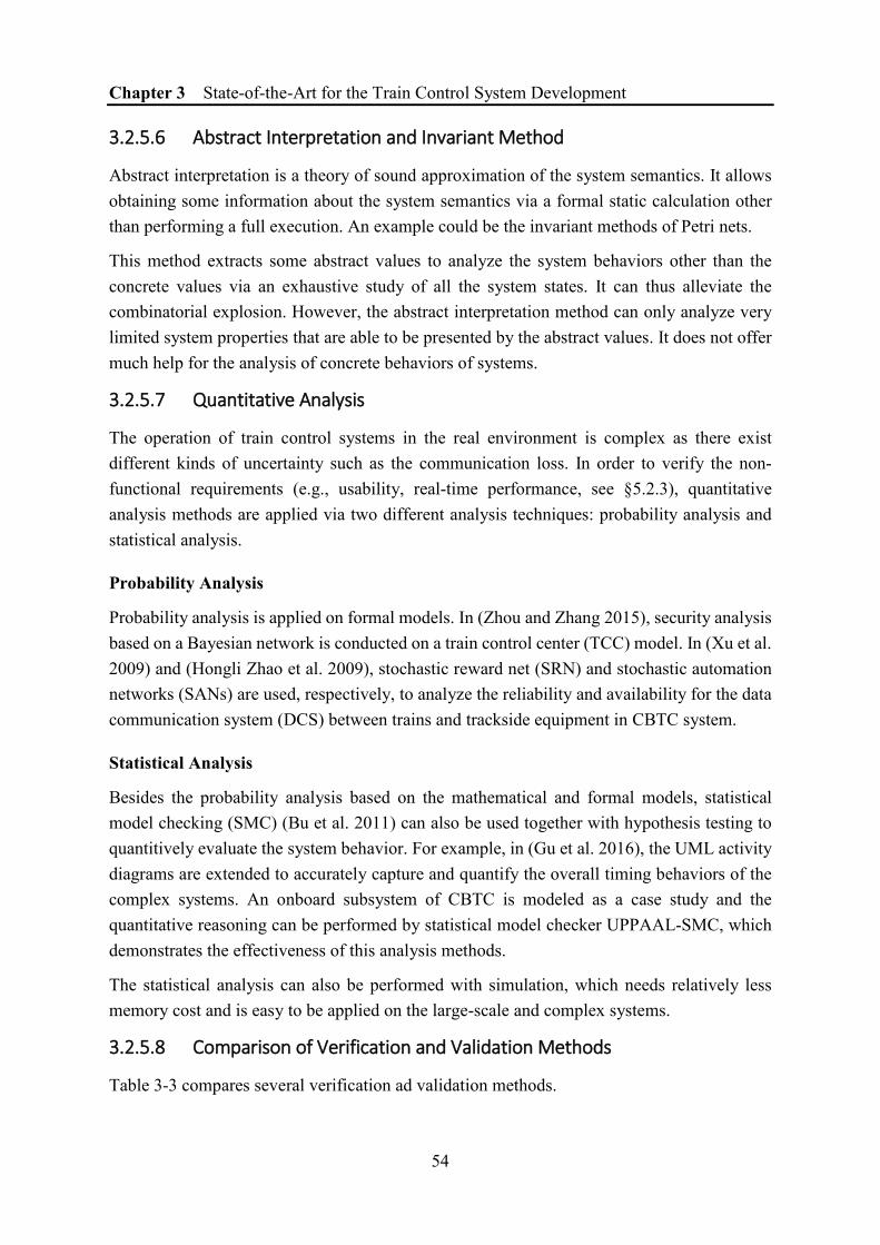
Chapter 3 State-of-the-Art for the Train Control System Development
54
3.2.5.6 Abstract Interpretation and Invariant Method
Abstract interpretation is a theory of sound approximation of the system semantics. It allows obtaining some information about the system semantics via a formal static calculation other than performing a full execution. An example could be the invariant methods of Petri nets.
This method extracts some abstract values to analyze the system behaviors other than the concrete values via an exhaustive study of all the system states. It can thus alleviate the combinatorial explosion. However, the abstract interpretation method can only analyze very limited system properties that are able to be presented by the abstract values. It does not offer much help for the analysis of concrete behaviors of systems.
3.2.5.7 Quantitative Analysis
The operation of train control systems in the real environment is complex as there exist different kinds of uncertainty such as the communication loss. In order to verify the non-functional requirements (e.g., usability, real-time performance, see §5.2.3), quantitative analysis methods are applied via two different analysis techniques: probability analysis and statistical analysis.
Probability Analysis
Probability analysis is applied on formal models. In (Zhou and Zhang 2015), security analysis based on a Bayesian network is conducted on a train control center (TCC) model. In (Xu et al. 2009) and (Hongli Zhao et al. 2009), stochastic reward net (SRN) and stochastic automation networks (SANs) are used, respectively, to analyze the reliability and availability for the data communication system (DCS) between trains and trackside equipment in CBTC system.
Statistical Analysis
Besides the probability analysis based on the mathematical and formal models, statistical model checking (SMC) (Bu et al. 2011) can also be used together with hypothesis testing to quantitively evaluate the system behavior. For example, in (Gu et al. 2016), the UML activity diagrams are extended to accurately capture and quantify the overall timing behaviors of the complex systems. An onboard subsystem of CBTC is modeled as a case study and the quantitative reasoning can be performed by statistical model checker UPPAAL-SMC, which demonstrates the effectiveness of this analysis methods.
The statistical analysis can also be performed with simulation, which needs relatively less memory cost and is easy to be applied on the large-scale and complex systems.
3.2.5.8 Comparison of Verification and Validation Methods
Table 3-3 compares several verification ad validation methods.

Chapter 3 State-of-the-Art for the Train Control System Development
55
3.2.6 Whole lifecycle tools
Many formal methods that we have introduced can contribute to different phases in the train control system development to support their requirements specification, system design, verification and validation. However, most of these methods are suited to a particular phase in the system development lifecycle. Since the different formal methods are based on different theories, the transition between the formal models in different phases could sometimes be an obstacle.
For example, even though that the requirements specification can be modeled and verified by some formal methods, the transformation into the system design model is usually conducted manually, which needs a lot of human labor by the experts with a good understanding of both the domain knowledge and the modeling techniques.
There might not exist a particular method which can cover all the modeling and verification in all the phases, but we have found some tools that could apply some formal methods to cover the most the phases and can thus be called “whole lifecycle tools”.
3.2.6.1 Rodin Based on Event-B
As the B method was proven to be useful in the maturity assessment of railway control domain (Behm et al. 1999), there are many studies about using B method and its successor Event-B to assist the system development of railway control. The use of B method / Event-B is extended from requirements specification modeling to other system development phases. Meanwhile, there are also tentative results of using model checking methods to verify its models besides the inherent theorem proving approach.
The toolset Rodin offers a basis of a User Interface (UI) and a proving engine for modeling and verification with Event-B. It is also compatible with several plug-ins for visualization, modeling and verification purposes. For all these reasons we regard Rodin as a whole lifecycle development tool based on Event-B.
More examples of the system development using Event-B and Rodin can be found in (Romanovsky and Thomas 2013).
The limit of these methods is that the B method is more appropriate to model the requirements specification. Even though there are methods to extend its applicable scope, the development needs to begin from a well-written formal requirements specification in Event-B. As for the verification, the model checking method is less well supported compared to the theorem proving, even though the former is more applicable in the industrial domain.
56
Table 3-3 Comparison of verification and Validation Methods
Type Method Phase(s) Principle Reliability Automation Expressivity C. E.
Traditional
Inspection R. / D. Reading Low Low
High Low Testing All phases General Middle Middle
Simulation D. / I. Execution Middle High
Formal
Model checking D. / I. Traversal High High High High
Theorem Proving R. / D. Reasoning High Low Low Middle
Abstract Interpretation R. / D. Calculation High Low Low Low
Equivalence checking D. / I. Logical analysis High High High High
Quantitative Analysis
Probability Analysis R. / D. Stochastic analysis High Middle Middle High
Statistical Analysis D. / I. Execution Middle High High Low
Abbreviations: R. – Requirements Specification; D. – System Design; I. – Implementation; C.E. - Combinatorial Explosion
Chapter 3 State-of-the-Art for the Train Control System Development
57
3.2.6.2 SCADE Suite
SCADE Suite (Safety-Critical Application Development Environment) is a whole lifecycle and high-quality system design solution of a model-based development environment for critical embedded software.
With the native integration of the well-defined SCADE language based on the formal language Lustre, SCADE Suite supports different representations of the target system, e.g., a graphical and hierarchical Safe State Machine (SSM) which can be mixed with the data flow, arrays and iterators. SCADE Suite offers a complete toolchain to undertake the prototyping, modeling, simulation, verification, optimization, and certified code generation for embedded systems controls, logic and algorithm designs.
In (Cho et al. 2011), ATP and ATO functions for CBTC onboard systems are designed with SCADE. Some functions are then tested using the SCADE simulator. As for implementation, C code is generated by KCG, a C-code generator certified by the EN 50128 standard.
However, as a commercial software developed by Esterel Technologie, a subsidiary of Ansys, Inc., SCADE Suite is very expensive and needs to be paid each year. As an academic research, the focus of this thesis is more oriented to the free or open source tools which can guarantee a reliable support for the long-term system development such as that of railway systems.
3.2.6.3 CPN Tools based on Petri nets
Compared to the B-Method which is appropriate for sequential software, Petri nets have been successfully applied for concurrent systems (Choppy and Petrucci 2004) thanks to its combination of a graphic representation and a formal and mathematical base. The expressivity of Petri nets is dramatically increased by the use of high-level Petri nets or colored Petri nets.
CPN Tools (Ratzer, A. et al., 2003) is a free software and a powerful tool based on colored Petri nets theory. It is especially useful for industrial application as its graphical representation allows the data flow and the control flow to be visualized, making it much easier for domain experts to understand system behavior.
CPN Tools combines the colored Petri nets theory with several extensions, e.g., the programming language ML (Jensen 1998), to gain an enhanced expressivity.
CPN theory offers:
- Petri net primitives of parallelism useful for the synchronization of concurrent processes, which is always a drawback of automata-based methods;
- high-level abstraction and hierarchy, which makes it possible to model large-scale and complex DES;
- the well-developed Petri net theory, which is supported by many tools and methods and is still being enriched.

Chapter 3 State-of-the-Art for the Train Control System Development
58
ML programming language provides:
- a definition of complex data types;
- the manipulation of data values via sophisticated functions and algorithm;
- the access to the integrated model checker and other CPN Tools functions.
As a whole lifecycle development tool, CPN Tools offers:
- a graphical environment to construct CPN models; - a simulator with debugging (e.g., stop conditions) for the testing and validation; - the generation of full state space, partial state space and condensed state space - the standard analysis and ASK-CTL (Cheng A. et al., 1996) based model checking,
which can be conducted to achieve a functional verification (She et al. 2014); - the support of PNML (Petri Net Markup Language), which makes it possible to reuse
the models in other tools;
All these features make CPN Tools a powerful tool with which we can design, simulate and analyze the models based on colored Petri nets during the whole development lifecycle for distributed and parallel systems where concurrency is an important characteristic.
In the requirements specification phase, the system requirements represented in CPN models is subjected to analysis methods to prove properties (ISO/IEC 2004). In the system design phase, the execution of CPN models allows the testing, simulation, and performance analysis on prototypes or design models before implementation. Meanwhile, in the implementation phase, code generation is also possible from CPN models (Mortensen 2000; Espensen et al. 2009; Kristensen and Westergaard 2010; Simonsen and Kristensen 2014).
More introduction to CPN Tools can be found in §3.3.3.4
3.2.6.4 RAISE development method
RAISE stands for Rigorous Approach to Industrial Software Engineering. It is a formal method originally created by Anne Haxthausen in Technical University of Denmark (Haxthausen et al. 1993). RAISE provides facilities for the use of formal methods in industrial software development. It supports the system design modeling from RSL, the RAISE Specification Language and is suitable to model concurrent and distributed systems such as train control systems (Haxthausen and Peleska 2000; Madsen and Bæk 2005).
In (Haxthausen and Peleska 2000), a distributed railway control system is designed and verified with RAISE. Derived from abstract requirements, the concrete safety specification is generated and its soundness and completeness are validated. In order to reduce the complexity, a domain model and a controller model are used to describe the system behavior. The domain model represents the physical system in absence of control, meanwhile, the controller model

Chapter 3 State-of-the-Art for the Train Control System Development
59
serves as a monitor of the domain model to decide whether it is safe for a train to move or for a point to be switched based on a safety-related control mechanism.
For the moment, two RAISE tools are developed:
• eden: the original core toolset for SUN workstations which requires the user to have both a deep knowledge of programming and the RSL (Dandanell et al. 1993) ;
• rsltc: a RAISE tool for Windows and Linux which is designed to be used from the command line or from an EMACS editor. After 2013 an Eclipse plugin eRAISE for rsltc is available but with limited support for only an essential subset of the rsltc functions, e.g., syntax and type checking, conversion to LaTeX, translation to SML, execution of test cases (Fasie 2013).
In a word, the RAISE tool is promising but for the moment less matured compared to the other whole lifecycle development methods to be applied in the industrial domains.
3.2.6.5 Comparison of whole lifecycle tools
The four whole lifecycle tools introduced in this section are compared in Table 3-4.
Table 3-4 Comparison of whole lifecycle tools
Tools Modeling Verification Major limits
Rodin Event-B Theory proving Need to begin from formal
specifications
SCADE Suite SSM + Lustre Interactive simulation, Symbology verification
Commercial software
RAISE RSL Theory proving,
Informal verification Limited tool support
which is not graphical
CPN Tools CPN + ML Simulation,
Model checking Combinatorial explosion
in model-checking
3.3 Petri Nets
On the basis of the previous discussion, we have chosen Petri nets as the formalism to model and verify the train control systems in this study.
In this section, with a classification of Petri nets variants we introduce two important Petri nets variants, CPN and WFN, that we used in this study to build the models. CPN Tools is also emphasized as it is the main modeling and verification tool used in this thesis.
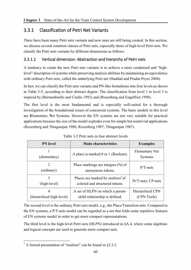
Chapter 3 State-of-the-Art for the Train Control System Development
60
3.3.1 Classification of Petri Net Variants
There have been many Petri nets variants and new ones are still being created. In this section, we discuss several common classes of Petri nets, especially those of high-level Petri nets. We classify the Petri nets variants by different dimensions as follows.
3.3.1.1 Vertical dimension: Abstraction and hierarchy of Petri nets
A tendency to create the new Petri nets variants is to achieve a more condensed and “high-level” description of systems while preserving analysis abilities by maintaining an equivalence with ordinary Petri nets, called the underlying Petri net (Haddad and Pradat-Peyre 2004).
In fact, we can classify the Petri nets variants and PN-like formalisms into four levels as shown in Table 3-5, according to their abstract degree. The classification from level 1 to level 3 is inspired by (Bernardinello and Cindio 1992) and (Rozenberg and Engelfriet 1998).
The first level is the most fundamental and is especially well-suited for a thorough investigation of the foundational issues of concurrent systems. The basic models in this level are Elementary Net Systems. However the EN systems are not very suitable for practical applications because the size of the model explodes even for simple but nontrivial applications (Rozenberg and Thiagarajan 1986; Rozenberg 1987; Thiagarajan 1987).
Table 3-5 Petri nets in four abstract levels
PN level Main characteristics Examples
1 (elementary)
A place is marked 0 or 1 (Boolean). Elementary Net
Systems
2 (ordinary)
Place markings are integers (ℕ) of anonymous tokens.
P/T-nets
3 (high-level)
Places are marked by multiset*of colored and structured tokens.
Pr/T-nets; CP-nets
4 (hierarchical high-level)
A set of HLPN on which a parent-child relationship is defined.
Hierarchical CPN (CPN Tools)
The second level is the ordinary Petri nets model, e.g., the Place/Transition-nets. Compared to the EN systems, a P/T-nets model can be regarded as a net that folds some repetitive features of EN systems model in order to get more compact representations.
The third level is the high-level Petri nets (HLPN) introduced in §A.4, where some algebraic and logical concepts are used to generate more compact nets.
* A formal presentation of “multiset” can be found in §3.3.2.

Chapter 3 State-of-the-Art for the Train Control System Development
61
Finally, the fourth level uses the concept of hierarchy (Huber et al. 1991; Buchholz 1994) to create a hierarchical high-level Petri net (HHPN). HHPN further “folds” the high-level Petri nets in a new dimension. If we regard the folding from ordinary PN to HLPN as a “flat” folding, the abstraction used in HHPN is somehow vertical by the reuse of sub-nets.
It is worth noting that the “folding” of Petri nets to higher level itself is entirely backward compatible with the original Petri nets. That is to say, a Petri net in a higher level in Table 3-5 can always be “unfolded” to a lower-level model while maintaining exactly the same modeling semantics and behaviors.
HHPN are suited to model complex systems. However, the hierarchy can be implemented by different techniques in order to substitute the subnets. For example, in (Bouyakoub and Belkhir 2008) the substitution is based on place, while in (Mascheroni 2010) the path concept is introduced to represent the hierarchy. In this study, the CPN Tools models are hierarchical models where the substitution transitions are used to replace the subsets in the higher level. More modeling details in CPN Tools will be further introduced later.
It is worth noting that even though the hierarchy concept has Significant results when it is used with high-level Petri nets, it can also be applied with ordinary (low-level) Petri nets.
3.3.1.2 Horizontal dimension: Extensions of Petri net
An important motivation for the introduction of new Petri nets classes is to enhance the expressive power of Petri nets models. Before a new revolutionary net would appear, most variants are obtained by adding extensions to the basic Petri nets to enhance the expressivity in a particular aspect according to the different applications.
Some examples of extensions are:
• Time constraints (Camurri et al. 1991; Reinaldo and del Foyo 2012);
• Stochastic properties (Balbo 2001) for performance evaluation;
• Reset arc, inhibitor arc and capacity limit (Bedők 2016), which add limits to the basic firing rules;
• Prioritized transitions (Guan et al. 1998; Westergaard and Verbeek 2011) which changes the token-game semantics;
• Algebraic Petri-nets (Best et al. 2001) and Concurrent OO Petri Nets (Agha et al. 2001) based on the former, both enable the use of algebraic and more data types;
• More exertions can be found in (He and Murata 2005).
The definition and application of extensions will facilitate the modeling process. However, the execution, simulation, and analysis of these Petri nets with extensions always require specialized tools that are compatible with these extensions.

Chapter 3 State-of-the-Art for the Train Control System Development
62
3.3.1.3 Ease of theoretical analysis
The use of high-level Petri nets facilitates the modeling phase of complex DES as the models can be compact and well-structured. However, it also brings the burden to the analysis phase.
Most analysis methods have been designed for ordinary Petri nets (Place/Transition-nets). The analysis of other Petri nets variants is faced with two problems.
- For high-level Petri nets which are obtained via abstraction and especially those with hierarchy, although one can always apply the general analysis methods after an unfolding process, the application of these methods is at risk of combinatorial explosion problem during the unfolding process;
- For a Petri net class created with some extensions (which is usually the case to achieve the modeling facility in some specialized areas), the extensions may bring some difficulties to unfold and analyze the high-level models using the traditional methods.
In short, the enhancement of the modeling power usually increases the difficulty for analysis.
In this context, some high-level Petri nets variants with the aim of “ease of analysis” are proposed with some modeling constraints on the basic of HLPN, in order to have a better compatibility with the (formal) analysis methods, which is somehow on the contrary of the import of extensions.
The advantage of these variants is that they are designed to bring a good eligibility for some direct analysis or reduction methods on the high-level Petri nets models.
A good example is the well-formed colored Petri nets (WFN) (Chiola et al. 1991a), where different constraints are defined on the colorsets (domains) for places, on the guards for transition, and on the functions for arc-inscriptions. More details are introduced in §3.3.2.4.
Compared to the basic high-level Petri nets, the WFN, on the one hand, allows the common high-level modeling for general purpose to have a compact model; on the other hand, ensures the accessibility to a series of formal analysis methods and are free-tuned to allow efficient use of various analysis tools. (Brgan and Poitrenaud 1995; Haddad et al. 1995).
Another similar example of high-level Petri net for ease of analysis could be Symmetric Nets (Haddad et al. 2009; Colange et al. 2011).
3.3.2 Colored Petri Net (CPN)
In this section, we introduce a Petri net variant which is broadly used today — Colored Petri Nets. The notation used in this section can be referred to (Jensen and Kristensen 2009a).
It is worth noting that there exist different variants of colored Petri nets, which is quite confusing (a detailed and interesting discussion can be found in §A.5). In order to avoid the
Chapter 3 State-of-the-Art for the Train Control System Development
63
confusion in this thesis, we tacitly use the abbreviations and notations as follows if they appear without a clear illustration by the context:
• CP-nets, for the original version of “colored Petri nets” in (Jensen 1981a);
• CPN, for the popularly spread graphical representation of “Colored Petri Nets” in (Jensen and Kristensen 2009a);
• CPN (enhanced with CPN Tools), for the CPN implementation by CPN Tools with CPN ML, hierarchy, and other extensions supported by this tool.
3.3.2.1 Multiset
Multiset needs to be defined before we can understand the CPN definition.
A multiset is a generalized type of set with multiple occurrences of the set elements. Let 𝑆𝑆 ={𝑠𝑠1, 𝑠𝑠2, 𝑠𝑠3, ⋯ } be a non-empty set. Then a multiset over 𝑆𝑆 is a function 𝑚𝑚 ∶ 𝑆𝑆 → 𝑁𝑁 mapping each element 𝑠𝑠 ∈ 𝑆𝑆 into a non-negative integer 𝑚𝑚(𝑠𝑠) ∈ 𝑁𝑁, i.e., the coefficient of 𝑠𝑠 in 𝑚𝑚.
In other words, a multiset 𝑚𝑚 can be written in the form of a sum:
� 𝑚𝑚(𝑠𝑠)`𝑠𝑠 = 𝑚𝑚(𝑠𝑠1)`𝑠𝑠1 + +𝑚𝑚(𝑠𝑠2)`𝑠𝑠2 + +𝑚𝑚(𝑠𝑠3)`𝑠𝑠3 + + ⋯�∈�
++ (3-1)
We use a special character – “grave accent” character ( ` ) – to explicitly indicate the relation between the coefficient and the set element. This expression is also a convention in Kurt Jensen’s Colored Petri Nets related research and is used by some software like CPN Tools.
The operator “+ +” means the addition operation of multisets (to distinguish from numbers).
The notation 𝑆𝑆�� is an infinite set containing all multisets over S and ∅�� , the empty multiset.
Other details and operations of multiset can be found in (Jensen and Kristensen 2009a).
3.3.2.2 Syntax of CPN
There are different versions of definitions of CPN. In this thesis, we refer to the definition 4.2 in (Jensen and Kristensen 2009a).
Definition 3-1 A non-hierarchical Colored Petri Net is a 9-tuple 𝐶𝐶𝐶𝐶𝑁𝑁 = <𝐶𝐶, 𝑇𝑇, 𝐴𝐴, 𝛴𝛴, 𝑉𝑉, 𝐶𝐶, 𝐺𝐺, 𝐸𝐸, 𝐼𝐼 > which contains:
• Net structure definitions:
- 𝐶𝐶 is a finite set of places;
- 𝑇𝑇 is a finite set of transitions, and 𝐶𝐶 ∩ 𝑇𝑇 ≠ ∅;
- 𝐴𝐴 ⊆ 𝐶𝐶 × 𝑇𝑇 ∪ 𝑇𝑇 × 𝐶𝐶 is a set of directed arcs;
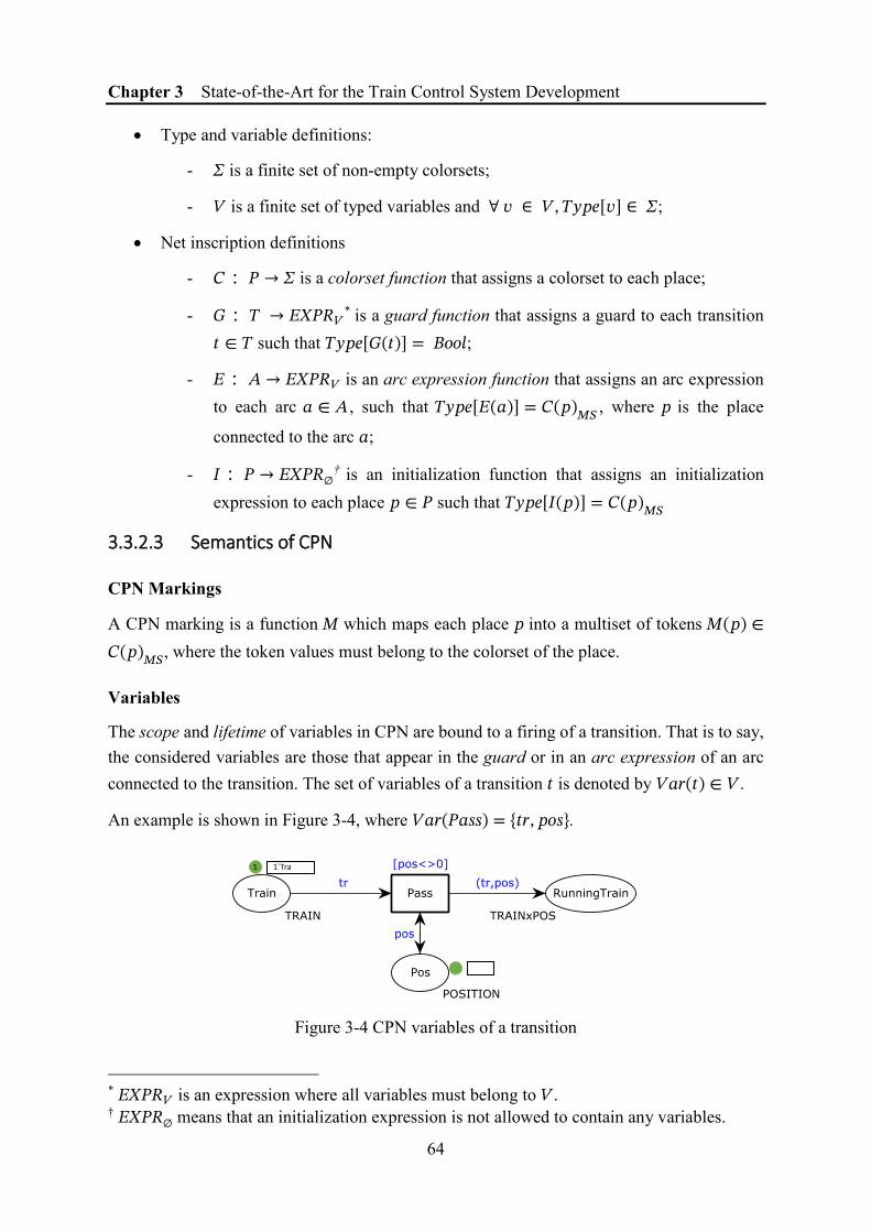
Chapter 3 State-of-the-Art for the Train Control System Development
64
• Type and variable definitions:
- 𝛴𝛴 is a finite set of non-empty colorsets;
- 𝑉𝑉 is a finite set of typed variables and ∀ 𝑣𝑣 ∈ 𝑉𝑉, 𝑇𝑇𝑇𝑇𝑇𝑇𝑇𝑇[𝑣𝑣] ∈ 𝛴𝛴;
• Net inscription definitions
- 𝐶𝐶 ∶ 𝐶𝐶 → 𝛴𝛴 is a colorset function that assigns a colorset to each place;
- 𝐺𝐺 ∶ 𝑇𝑇 → 𝐸𝐸𝐸𝐸𝐶𝐶𝐸𝐸�* is a guard function that assigns a guard to each transition
𝑡𝑡 ∈ 𝑇𝑇 such that 𝑇𝑇𝑇𝑇𝑇𝑇𝑇𝑇[𝐺𝐺(𝑡𝑡)] = 𝐵𝐵𝐵𝐵𝐵𝐵𝐵𝐵;
- 𝐸𝐸 ∶ 𝐴𝐴 → 𝐸𝐸𝐸𝐸𝐶𝐶𝐸𝐸� is an arc expression function that assigns an arc expression to each arc 𝑎𝑎 ∈ 𝐴𝐴 , such that 𝑇𝑇𝑇𝑇𝑇𝑇𝑇𝑇[𝐸𝐸(𝑎𝑎)] = 𝐶𝐶(𝑇𝑇)�� , where 𝑇𝑇 is the place
connected to the arc 𝑎𝑎;
- 𝐼𝐼 ∶ 𝐶𝐶 → 𝐸𝐸𝐸𝐸𝐶𝐶𝐸𝐸∅† is an initialization function that assigns an initialization
expression to each place 𝑇𝑇 ∈ 𝐶𝐶 such that 𝑇𝑇𝑇𝑇𝑇𝑇𝑇𝑇[𝐼𝐼(𝑇𝑇)] = 𝐶𝐶(𝑇𝑇)��
3.3.2.3 Semantics of CPN
CPN Markings
A CPN marking is a function 𝑀𝑀 which maps each place 𝑇𝑇 into a multiset of tokens 𝑀𝑀(𝑇𝑇) ∈𝐶𝐶(𝑇𝑇)��, where the token values must belong to the colorset of the place.
Variables
The scope and lifetime of variables in CPN are bound to a firing of a transition. That is to say, the considered variables are those that appear in the guard or in an arc expression of an arc connected to the transition. The set of variables of a transition 𝑡𝑡 is denoted by 𝑉𝑉𝑎𝑎𝑉𝑉(𝑡𝑡) ∈ 𝑉𝑉.
An example is shown in Figure 3-4, where 𝑉𝑉𝑎𝑎𝑉𝑉(𝐶𝐶𝑎𝑎𝑠𝑠𝑠𝑠) = {𝑡𝑡𝑉𝑉, 𝑇𝑇𝐵𝐵𝑠𝑠}.
Figure 3-4 CPN variables of a transition
* 𝐸𝐸𝐸𝐸𝐶𝐶𝐸𝐸� is an expression where all variables must belong to 𝑉𝑉. † 𝐸𝐸𝐸𝐸𝐶𝐶𝐸𝐸∅ means that an initialization expression is not allowed to contain any variables.
1 1`Trai

Chapter 3 State-of-the-Art for the Train Control System Development
65
Bindings and binding elements
A binding of a transition 𝑡𝑡 is a function 𝑏𝑏 that maps each variable 𝑣𝑣 ∈ 𝑉𝑉𝑎𝑎𝑉𝑉(𝑡𝑡) into a value 𝑏𝑏(𝑣𝑣) ∈ 𝑇𝑇𝑇𝑇𝑇𝑇𝑇𝑇[𝑣𝑣]. All the bindings for a transition 𝑡𝑡 can be denoted as a set 𝐵𝐵(𝑡𝑡).
A binding is always written in angle brackets, e.g., a binding of transition Pass in Figure 3-4 could be ⟨𝑡𝑡𝑉𝑉 = 𝑇𝑇𝑉𝑉𝑎𝑎𝑇𝑇𝑇𝑇(1), 𝑇𝑇𝐵𝐵𝑠𝑠 = 1⟩.
A binding element is a pair (𝑡𝑡, 𝑏𝑏) which combines a transition 𝑡𝑡 to a binding 𝑏𝑏 ∈ 𝐵𝐵(𝑡𝑡), which assigns values for the variables in the surroundings of a transition 𝑡𝑡, i.e., 𝑉𝑉𝑎𝑎𝑉𝑉(𝑡𝑡).
All the binding elements of a transition 𝑡𝑡 is denoted as a set 𝐵𝐵𝐸𝐸(𝑡𝑡). And the set of all binding elements in a CPN is denoted as 𝐵𝐵𝐸𝐸.
Enabling and occurrence of a single binding element
The rules for enabling an occurrence of a single binding element in CPN are based on evaluations of guards and arc expressions, which are:
• 𝐺𝐺(𝑡𝑡)⟨𝑏𝑏⟩, the evaluation of a guard expression for transition 𝑡𝑡 with the binding 𝑏𝑏;
• 𝐸𝐸(𝑎𝑎)⟨𝑏𝑏⟩, the evaluation of the arc expression on an arc 𝑎𝑎 with the binding 𝑏𝑏;
• 𝐸𝐸(𝑇𝑇, 𝑡𝑡)⟨𝑏𝑏⟩, the evaluation of the arc expression on the arc from place 𝑇𝑇 to transition 𝑡𝑡, with the binding 𝑏𝑏. If such an arc does not exist, then 𝐸𝐸(𝑇𝑇, 𝑡𝑡)⟨𝑏𝑏⟩ = ∅��;
• 𝐸𝐸(𝑡𝑡, 𝑇𝑇)⟨𝑏𝑏⟩, the evaluation of the arc expression on the arc from transition 𝑡𝑡 to place 𝑇𝑇, with the binding 𝑏𝑏. If such an arc does not exist, then 𝐸𝐸(𝑡𝑡, 𝑇𝑇)⟨𝑏𝑏⟩ = ∅��.
A binding element (𝑡𝑡, 𝑏𝑏) ∈ 𝐵𝐵𝐸𝐸 is said to be enabled in a marking 𝑀𝑀 iff the following two
conditions are fulfilled:
• 𝐺𝐺(𝑡𝑡)⟨𝑏𝑏⟩ = 𝑡𝑡𝑉𝑉𝑡𝑡𝑇𝑇;
• For all 𝑇𝑇 ∈ 𝐶𝐶, 𝐸𝐸(𝑇𝑇, 𝑡𝑡)⟨𝑏𝑏⟩ ≤ 𝑀𝑀(𝑇𝑇)*.
When a binding element (𝑡𝑡, 𝑏𝑏) ∈ 𝐵𝐵𝐸𝐸 is enabled in a marking M, it may occur, which will then lead to a new marking 𝑀𝑀′ where for all 𝑇𝑇 ∈ 𝐶𝐶,
𝑀𝑀′(𝑇𝑇) = (𝑀𝑀(𝑇𝑇) − −𝐸𝐸(𝑇𝑇, 𝑡𝑡)⟨𝑏𝑏⟩) + + 𝐸𝐸(𝑡𝑡, 𝑇𝑇)⟨𝑏𝑏⟩. (3-2)
Enabling and occurrence of step
We define a step 𝑌𝑌 ∈ 𝐵𝐵𝐸𝐸�� as a non-empty and finite multiset of binding elements.
* The operator (for integer) “≤” is overloaded to mean “smaller than or equal” for multisets.

Chapter 3 State-of-the-Art for the Train Control System Development
66
A step 𝑌𝑌 ∈ 𝐵𝐵𝐸𝐸�� is said to be enabled in a marking M iff the following two conditions are
fulfilled:
• For all (𝑡𝑡, 𝑏𝑏) ∈ 𝑌𝑌, 𝐺𝐺(𝑡𝑡)⟨𝑏𝑏⟩ = 𝑡𝑡𝑉𝑉𝑡𝑡𝑇𝑇;
• For all 𝑇𝑇 ∈ 𝐶𝐶, ∑ 𝐸𝐸(𝑇𝑇, 𝑡𝑡)⟨𝑏𝑏⟩(�,�)∈���
++ ≤ 𝑀𝑀(𝑇𝑇)*.
When a step Y ∈ 𝐵𝐵𝐸𝐸�� is enabled in a marking M, it may occur, which will then lead to a new marking 𝑀𝑀′ where for all 𝑇𝑇 ∈ 𝐶𝐶,
𝑀𝑀′(𝑇𝑇) = 𝑀𝑀(𝑇𝑇) − − ∑ 𝐸𝐸(𝑇𝑇, 𝑡𝑡)⟨𝑏𝑏⟩ + +(�,�)∈���
++ ∑ 𝐸𝐸(𝑡𝑡, 𝑇𝑇)⟨𝑏𝑏⟩(�,�)∈���
++ . (3-3)
Some notations about enabling and occurrence of step with markings are:
• 𝑀𝑀1�→ 𝑀𝑀2 , which means that step Y occurs in marking 𝑀𝑀1 and leads to marking M2;
• M1 → 𝑀𝑀2, which means that marking M2 can be reached from marking M1 by the occurrence of an unknown step;
• 𝑀𝑀1�→ , which means that step Y is enabled in marking M1 (and leads to an unknown
marking).
Occurrence sequence
A finite occurrence sequence (of step) is defined as:
𝑀𝑀1�1→ 𝑀𝑀2
�2→ 𝑀𝑀3 ⋯ ⋯ 𝑀𝑀�
��→ 𝑀𝑀�+1 (3-4)
where n is said to be its length and n ≥ 0.
In (3-4), all markings presented in the sequence are reachable from M1. Each marking is also
reachable from itself by an occurrence sequence of length 0.
An infinite occurrence sequence (of step) is defined as:
𝑀𝑀1�1→ 𝑀𝑀2
�2→ 𝑀𝑀3 ⋯ ⋯. (3-5)
We denote ℛ(M) the set of markings reachable from M.
3.3.2.4 CPN Tools and CPN Extensions
The latest developments of colored Petri nets can be classified into two dimensions:
* ∑ ��
++ means the sum over a multiset.

Chapter 3 State-of-the-Art for the Train Control System Development
67
- the improvement to colored Petri net theory;
- the versatility and practicability to apply colored Petri nets in complex industrial systems design.
CPN Tools (Ratzer et al. 2003) is developed in Eindhoven University of Technology and is aimed at the practical use of CPN in industrial applications. CPN Tools was developed from Design/CPN, the first computer-based tool for editing, simulation and state-space analysis of colored Petri nets.
CPN Tools integrates the CPN theory with several extensions and features to widen its application in the industry. These extensions and features include:
• CPN ML (Jensen and Kristensen 2009b).
• Hierarchy in Colored Petri Nets (Huber et al. 1991);
• Time concept;
• Transition priority;
• Some special types e.g., a queuing place (syntactical sugar for the list construction, hence it does not alter the compatibility for simulation or state space analysis).
In our research, CPN Tools is used to build and analyze the train control system models. CPN Tools is efficient to be used in the modeling of large-scale and complex DES mainly thanks to the integration of CPN ML and the hierarchy.
CPN ML
CPN ML is based on the famous functional programming language Standard ML (Appel and MacQueen 1991; Milner et al. 1997). At the beginning of the development of CPN Tools, CPN ML was offered only to help specify types and net inscriptions, e.g., to declare colorsets, variables, and functions. In this context, the introduction of CPM ML was not an extension as it did not affect the general definition of CPN, which is independent of a concrete syntax and semantics for net inscriptions. Besides CPN ML there exists a number of other tools that use some other languages or methods to define types and net inscriptions.
However, we have noticed that the current version of CPN Tools has integrated much more features from ML language to enhance the expressive power of the models built using CPN Tools. For example, several types such as list type and their operations are not natively supported in CPN theory; ML code segment can be used to control the occurrence of transitions; file I/O operations make the nets’ behavior dependent on the environment… From this point of view, the use of CPN ML may affect the behavior of CPN and should thus be regarded an extension to CPN.
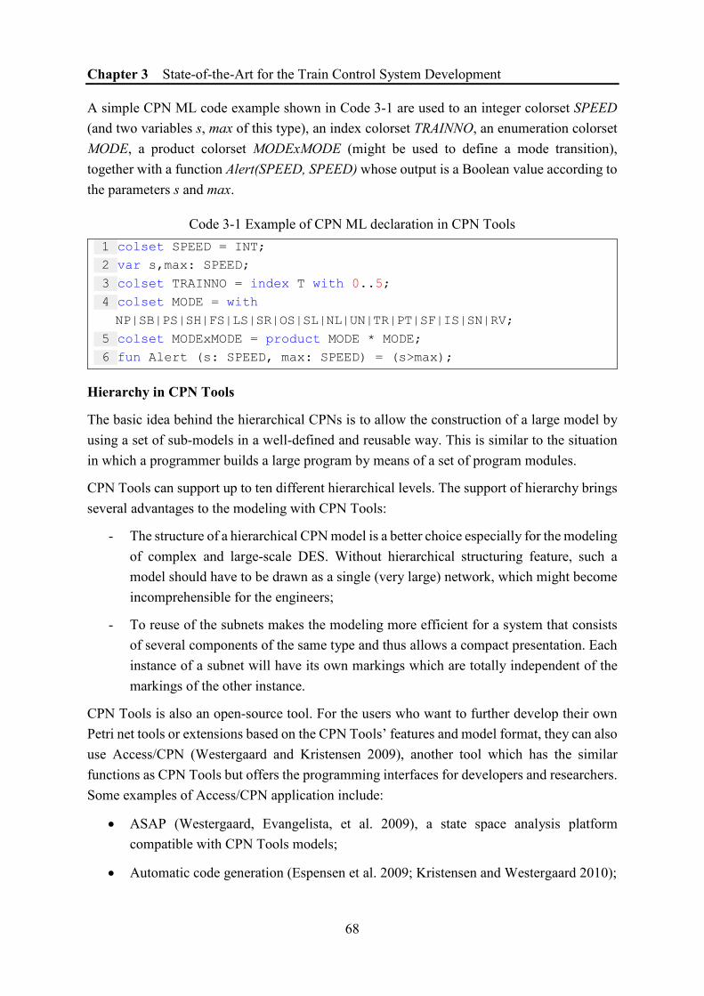
Chapter 3 State-of-the-Art for the Train Control System Development
68
A simple CPN ML code example shown in Code 3-1 are used to an integer colorset SPEED (and two variables s, max of this type), an index colorset TRAINNO, an enumeration colorset MODE, a product colorset MODExMODE (might be used to define a mode transition), together with a function Alert(SPEED, SPEED) whose output is a Boolean value according to the parameters s and max.
Code 3-1 Example of CPN ML declaration in CPN Tools 1 colset SPEED = INT; 2 var s,max: SPEED; 3 colset TRAINNO = index T with 0..5; 4 colset MODE = with
NP|SB|PS|SH|FS|LS|SR|OS|SL|NL|UN|TR|PT|SF|IS|SN|RV; 5 colset MODExMODE = product MODE * MODE; 6 fun Alert (s: SPEED, max: SPEED) = (s>max);
Hierarchy in CPN Tools
The basic idea behind the hierarchical CPNs is to allow the construction of a large model by using a set of sub-models in a well-defined and reusable way. This is similar to the situation in which a programmer builds a large program by means of a set of program modules.
CPN Tools can support up to ten different hierarchical levels. The support of hierarchy brings several advantages to the modeling with CPN Tools:
- The structure of a hierarchical CPN model is a better choice especially for the modeling of complex and large-scale DES. Without hierarchical structuring feature, such a model should have to be drawn as a single (very large) network, which might become incomprehensible for the engineers;
- To reuse of the subnets makes the modeling more efficient for a system that consists of several components of the same type and thus allows a compact presentation. Each instance of a subnet will have its own markings which are totally independent of the markings of the other instance.
CPN Tools is also an open-source tool. For the users who want to further develop their own Petri net tools or extensions based on the CPN Tools’ features and model format, they can also use Access/CPN (Westergaard and Kristensen 2009), another tool which has the similar functions as CPN Tools but offers the programming interfaces for developers and researchers. Some examples of Access/CPN application include:
• ASAP (Westergaard, Evangelista, et al. 2009), a state space analysis platform compatible with CPN Tools models;
• Automatic code generation (Espensen et al. 2009; Kristensen and Westergaard 2010);
Chapter 3 State-of-the-Art for the Train Control System Development
69
• Co-simulation of CPN models and SystemC programming language (Westergaard, Kristensen, et al. 2009)
• Integration of CPN models and process mining (Van Zelst et al. 2015)
3.3.3 Well-Formed Petri Nets and Symbolic Reachability Graph
3.3.3.1 The Trade-off between Expressiveness and Analysis Capability
As we have introduced in §3.3.1.3, a difficulty to choose a good formalism for the modeling and analysis of complex and large-scale DES is that a formalism with higher abstraction level and more extensions is usually more expressive but less friendly for the analysis and verification (Haddad et al. 2009).
For example, The CPN Tools models obtain an excellent expressiveness via very loose restraints on the types and functions, which is implemented with the help of ML programming language in CPN Tools. However, the analysis of these models is limited to the generation of state space. And the state space of these models may only be generated by CPN Tools, which can handle the ML definitions and functions. The reduction techniques and other analysis methods proposed for general CPNs are hence difficult, or even impossible to apply, which hampers its analysis capabilities.
In order to obtain a good trade-off between the expressiveness and the analysis capability, Regular Nets (Haddad 1987) have been proposed as a restriction on CP-nets (Jensen 1981a). With some constraints on the colorsets and on the arc expressions, it allows the computation of flows, net reductions and the application of symbolic reachability graph (SRG), which is normally more condensed than the whole state space and maintains the possibility for an exhaustive analysis (Chiola et al. 1997).
Well-Formed Petri Nets (WFN) were defined as an extension of Regular Nets to support more general classes like those in CPN. Thus, WFN can also be regarded as CPN that satisfies a set of syntactical constraints. These constraints are well designed so that the modeling power of WFN is said to be the same as the general CPN in spite of the use of all these constraints (Haddad et al. 1995). In (Chiola et al. 1991b; Chiola et al. 1993), it is pointed out that any general CPN can be represented by an equivalent WFN model with the same underlying structure with a rewrite of the color class definitions and color function expressions in a more explicit and parametric form according to the basic constructs provided by the WFN formalism.
In some more recent research, Well-formed Petri nets are also called Symmetric Nets (SN) with some subtle differences. For example, several variants such as Symmetric Nets with Bags (SNB) are proposed in Symmetric Nets (Haddad et al. 2009). In this thesis, we introduce WFN as a representative of this family of Petri net classes.

Chapter 3 State-of-the-Art for the Train Control System Development
70
WFN is useful to model a system where several instances (with different identifiers) of a same entity share the same behaviors, e.g., the dining philosophers problem (Ras 2016). When it comes to the verification phase, WFN allows the generation of SRG to support more efficient analysis algorithms based on the symbolic markings, which will be introduced later in §3.3.3.3.
While, according to our experience, WFN is still less convenient in practical use to model the large-scale and communication-based system with complex behaviors, such as the modern train control systems. In (Chiola et al. 1993), it was also said that “in practical modeling this translation (from CPN to WFN) is hardly needed and most (if not all) CPN models published in the literature can be directly represented as WFN even without exploiting several powerful formalisms provided by WFN, e.g., arc-labeling functions with predicate guards.” We believe that this statement is no longer true faced with the complexity of the practical modeling for the modern communication-based systems. Thus, in this study, we also propose several modeling patterns to facilitate the modeling of certain DES behavior in WFN (see §4.6).
3.3.3.2 Informal introduction to well-formed Petri nets
Since WFN is in fact a restriction on colored Petri nets (CPN) that we have introduced in §3.3.2. We will introduce the definition of WFN informally by emphasizing the differences (i.e., the constraints) compared with CPN. The complete formal definition can be found in (Chiola et al. 1991a; Chiola et al. 1991b; Chiola et al. 1993).
We first introduce some basic elements necessary for the WFN definition.
Basic Color Classes and Color Domains
Similar to CPN, a colored token in WFN incorporates some information. The “data type” associated with each place and each transition can be a basic color class or a color domain.
A basic color class is usually finite and defined by enumeration of its elements, as shown by the first line in (4-9). A neutral color is depicted as ε, maintaining the compatibility with uncolored Petri nets.
CLASS TRAIN = < t1, t2, t3, … , t10 >;
CLASS MSG = < m1, m2, m3 >∪< ack > DOMAIN TRAINxMSG = < TRAIN, MSG >.
(3-6)
A basic color class can be partitioned into a conjunction of several static subclasses. As shown by the second line in (4-9), a basic color class MSG is partitioned into two subclasses (which can be denoted by 𝐷𝐷���,1 and 𝐷𝐷���,2 ). Each static subclass usually defines a group of elements that share some common property. The terminology static subclass is used as opposite to dynamic subclass, which is another concept to define the symbolic marking in the analysis of WFN using SRG.

Chapter 3 State-of-the-Art for the Train Control System Development
71
A basic color class may be ordered or unordered. An ordered color class allows the use of the successor function which returns the next element. The details will be introduced later.
A color domain is a Cartesian product of several basic color classes (or, it can contain only one basic color class) as shown by the third line in (4-9). A color domain can be assigned to a transition or a place.
The color domain of a place 𝑇𝑇 is denoted ∁(𝑇𝑇). Similar to CPN, the marking of place 𝑇𝑇, denoted as 𝑀𝑀(𝑇𝑇), represents a multiset on ∁(𝑇𝑇) according to the marking 𝑀𝑀.
The color domain of a transition 𝑡𝑡 is denoted ∁(𝑡𝑡). It is a combination of all the color domains of its input and output places. A color 𝑐𝑐 ∈ ∁(𝑡𝑡) implies how the transition 𝑡𝑡 is fired. It is thus called a firing instance, which is similar to a (single) binding element in CPN (cf. §3.3.2). The relation between a firing instance of a transition 𝑡𝑡 and the tokens consume/generated of its input/output places is defined through the functions on the arc expressions, which will be introduced later.
Color functions
We denote the family of basic color classes of a WFN by C = {𝐶𝐶1, … , 𝐶𝐶ℎ, 𝐶𝐶ℎ+1, … , 𝐶𝐶�} where:
• 0 ≤ ℎ ≤ 𝑇𝑇,
• ∀ 𝑇𝑇 ≠ 𝑗𝑗 → 𝐶𝐶� ∩ 𝐶𝐶� = ∅,
• {𝐶𝐶1, … , 𝐶𝐶ℎ} are non-ordered classes and {𝐶𝐶ℎ+1, … , 𝐶𝐶�} are ordered classes
A transition color domain can be denoted as ∁(𝑡𝑡) = 𝐶𝐶1�1 × ⋯ × 𝐶𝐶�
�� where 𝑇𝑇� is the times of appearances* of a basic color class 𝐶𝐶� in ∁(𝑡𝑡). Correspondingly, a color 𝑐𝑐 ∈ ∁(𝑡𝑡) is denoted as 𝑐𝑐 = 𝑐𝑐1
�1 × ⋯ × 𝑐𝑐���.
Three kinds of basic functions on such a transition color domain ∁(𝑡𝑡) are defined:
- The identity function is denoted 𝐸𝐸��(𝑐𝑐) = 𝑐𝑐�
�, which selects the 𝑗𝑗�ℎ instance (1 ≤ 𝑗𝑗 ≤𝑇𝑇�) of a color element of 𝐶𝐶�. The identity function is also the basis of the following two basic functions. In practical use, an identity function is usually depicted by a variable (e.g. 𝐸𝐸, 𝑌𝑌) for short;
- The successor function ⊕ 𝐸𝐸�� returns successor† of the color element 𝐸𝐸�
�, supposing that the basic color class 𝐶𝐶� is an ordered class (i.e., h < i ≤ n). Given a variable X =
𝐸𝐸��, the successor function ⊕ Xi
j can also be denoted as X + 1;
* Note that if 𝑇𝑇� = 0, 𝐶𝐶� does not appear. † An ordered color class is always circular, so the successor function applied to the last color element returns the first one.

Chapter 3 State-of-the-Art for the Train Control System Development
72
- The diffusion function All(𝐸𝐸��) returns the multiset of all the colors elements of a basic
color class 𝐶𝐶� (if 𝐶𝐶� is not partitioned) or a static subclass D�,� (if 𝐶𝐶� is partitioned and
𝐸𝐸�� ∈ D�,�).
Color functions are formal sums of guarded functions built by standard operations (linear combination, composition, etc.) on the three basic functions.
Predicates and Guards
An atomic predicate may identify two variables ([X=Y]), compare a variable to another using successor function ([𝐸𝐸 =⊕ 𝑌𝑌]), or restrict a variable within a static subclass D ([X∈D]).
There are two scenes where the guards are used in WFN, i.e., the guarded transitions and the guarded functions. A guard is defined as a logical combination of atomic predicates.
Till now we have introduced the WFN formalisms from the three aspects above. Obviously, most of the techniques used in WFN are designed for the system symmetry. However, the static subclass partition and the use of guards also allow the representation of some asymmetric behaviors, which has strengthened the modeling power of WFN.
3.3.3.3 Symbolic Reachability Graph (SRG)
We use an example to illustrate the application of SRG.
Figure 3-5 shows a system comprised of 𝑇𝑇 identical processes (𝑇𝑇1, 𝑇𝑇2, … , 𝑇𝑇� ) in parallel, where each process has three local states (A, B, and C), the system may have 3� global states.
Figure 3-5 A system of n identical 3-states processes
If the 𝑇𝑇 processes are identical up to renaming, the state graph of such a system usually exhibits considerable symmetry. Taking an example of the system where 𝑇𝑇 = 2, its state space M contains 9 states shown in the first row of Table 3-6. A global state A{𝑇𝑇1}, B{𝑇𝑇2} represents the state where the process 𝑇𝑇1 is in its local state A while process 𝑇𝑇2 is in the local state B.
Two states A{𝑇𝑇1}, B{𝑇𝑇2} and A{𝑇𝑇2}, B{𝑇𝑇1} can be related by applying a permutation (1, 2) which changes the process index 1 to 2 and 2 to 1. The states after applying the permutation (1, 2) is shown in the second row of Table 3-6. It is easy to find that the transition of applying

Chapter 3 State-of-the-Art for the Train Control System Development
73
the permutation on M has resulted in M again, which means that the permutation (1, 2) is an automorphism of M.
Table 3-6 Example of state space reduction with symmetry
State Permutation (𝑇𝑇1, 𝑇𝑇2) applied Aggregated state
A{𝑇𝑇1, 𝑇𝑇2} A{𝑇𝑇1, 𝑇𝑇2} A{2}
A{𝑇𝑇1}, B{𝑇𝑇2} A{𝑇𝑇2}, B{𝑇𝑇1} A{1}, B{1}
A{𝑇𝑇2}, B{𝑇𝑇1} A{𝑇𝑇1}, B{𝑇𝑇2}
A{𝑇𝑇1}, C{𝑇𝑇2} A{𝑇𝑇2}, C{𝑇𝑇1} A{1}, C{1}
A{𝑇𝑇2}, C{𝑇𝑇1} A{𝑇𝑇1}, C{𝑇𝑇2}
B{𝑇𝑇1, 𝑇𝑇2} B{𝑇𝑇1, 𝑇𝑇2} B{2}
B{𝑇𝑇1}, C{𝑇𝑇2} B{𝑇𝑇2}, C{𝑇𝑇1} B{1}, C{1}
B{𝑇𝑇2}, C{𝑇𝑇1} B{𝑇𝑇1}, C{𝑇𝑇2}
C{𝑇𝑇1, 𝑇𝑇2} C{𝑇𝑇1, 𝑇𝑇2} C{2}
The states that are equivalent by applying a permutation are said to be symmetric and can be aggregated to an abstract state, as shown in the last row of Table 3-6. Aggregated states imply the general distribution of tokens rather than the concrete tokens with identifiers. The state space is thus reduced based on symmetry.
The use of symmetry to construct a reduced reachability graph of high-level Petri nets was first introduced in (Huber et al. 1986) with the symmetries defined by the modeler and the same firing rules as the ordinary Petri nets. Then the automatic detection of symmetries was introduced to colored Petri nets in (Junttila 2003) to achieve automatic symbolic verification.
In (Chiola et al. 1997), the construction of symbolic reachability graph (SRG) was proposed on well-formed Petri nets together with the symbolic firing rule. The construction can be automated by a general algorithm. Several Petri net tools such as GreatSPN (Chiola et al. 1995), CPN-AMI (Kordon and Paviot-Adet 1999) and Crocodile (Colange et al. 2011) can be used to construct and analyze WFN models, which will be later introduced in 3.3.3.4.
The equivalence of several structural properties (e.g., reachability, liveness and numerical properties) in SRG are proven. The model checking of general temporal logic formulas can be extended to the SRG (Emerson and Sistla 1996; Ilié and Ajami 1997). It is worth noting that the symmetry detection within ordinary Petri nets is also possible (Schmidt 2000).

Chapter 3 State-of-the-Art for the Train Control System Development
74
Even though the construction of SRG offers great potential to fight against the combinatorial explosion problem, there are some obstacles to applying this method in the modeling and verification of the train control systems.
Firstly, other than the demos and examples of protocols which are often used to show the interest of the symmetry, the global behavior of train control systems is not symmetric. Meanwhile, the design of train control systems may contain some symmetries somewhere. In (Emerson and Trefler 1999) and (Baarir et al. 2005), partially symmetric systems are studied and some verification and evaluation procedures are proposed on these partially symmetric models. However, there are not yet mature tools which can analyze the partial symmetry automatically, which makes it a huge amount of work to identify and separate the symmetric parts in the large-scale and complex system models.
Secondly, the modern train control systems are always communication-based systems with the support for Movement Authority (MA) management. When modeled with colored Petri nets, most of the behavior of these systems is rather based on the values other than the distribution of the colored tokens. In this case, it is always too difficult to take advantage of the symmetry.
3.3.3.4 Tools supporting WFN
GreatSPN (Chiola et al. 1995) is a Petri net modeling, validation, and performance evaluation tool developed by the University of Turin in cooperation with the University of Eastern Piedmont. It supports Generalized Stochastic Petri Nets (GSPN) and its high-level and well-formed version: Stochastic Well-formed Nets (SWN). For the latter, Symbolic Reachability Graph analysis is supported. GreatSPN supports time concept. It also implements several efficient analysis algorithms to facilitate complex system design and allows the analysis of models running on different machines in a distributed computing environment.
CPN-AMI (Kordon and Paviot-Adet 1999) is developed by LIP6 (French: Laboratoire d'Informatique de Paris 6) and supports well-formed Petri nets (WFN). It defines AMI-Net as a WFN implementation with a specific syntax. CPN-AMI allows users to build AMI-Net models, to analyze the structural and behavioral properties, and to unfold high-level Petri nets to Place/Transition-nets. It supports PNML format and can be used together with some other tools. However, it seems that the developer has stopped the support and update of this tool.
Crocodile (Colange et al. 2011) is another tool developed by LIP6, which takes CPN-AMI as a reference and supports Symmetric Nets (SN, similar to WFN) and Symmetric Nets with Bags (SNB).
It is worth noting that besides the tools who claim support of the well-formed Petri nets, one could also choose from a variety of tools for colored Petri nets and High-level Petri Nets to build their WFN models with respect to the WFN definition.
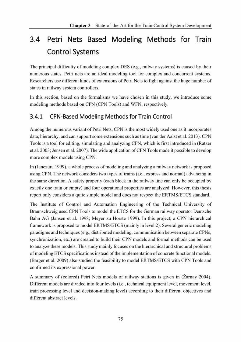
Chapter 3 State-of-the-Art for the Train Control System Development
75
3.4 Petri Nets Based Modeling Methods for Train Control Systems
The principal difficulty of modeling complex DES (e.g., railway systems) is caused by their numerous states. Petri nets are an ideal modeling tool for complex and concurrent systems. Researchers use different kinds of extensions of Petri Nets to fight against the huge number of states in railway system controllers.
In this section, based on the formalisms we have chosen in this study, we introduce some modeling methods based on CPN (CPN Tools) and WFN, respectively.
3.4.1 CPN-Based Modeling Methods for Train Control
Among the numerous variant of Petri Nets, CPN is the most widely used one as it incorporates data, hierarchy, and can support some extensions such as time (van der Aalst et al. 2013). CPN Tools is a tool for editing, simulating and analyzing CPN, which is first introduced in (Ratzer et al. 2003; Jensen et al. 2007). The wide application of CPN Tools made it possible to develop more complex models using CPN.
In (Janczura 1999), a whole process of modeling and analyzing a railway network is proposed using CPN. The network considers two types of trains (i.e., express and normal) advancing in the same direction. A safety property (each block in the railway line can only be occupied by exactly one train or empty) and four operational properties are analyzed. However, this thesis report only considers a quite simple model and does not respect the ERTMS/ETCS standard.
The Institute of Control and Automation Engineering of the Technical University of Braunschweig used CPN Tools to model the ETCS for the German railway operator Deutsche Bahn AG (Jansen et al. 1998; Meyer zu Hörste 1999). In this project, a CPN hierarchical framework is proposed to model ERTMS/ETCS (mainly in level 2). Several generic modeling paradigms and techniques (e.g., distributed modeling, communication between separate CPNs, synchronization, etc.) are created to build their CPN models and formal methods can be used to analyze these models. This study mainly focuses on the hierarchical and structural problems of modeling ETCS specifications instead of the implementation of concrete functional models. (Barger et al. 2009) also studied the feasibility to model ERTMS/ETCS with CPN Tools and confirmed its expressional power.
A summary of (colored) Petri Nets models of railway stations is given in (Žarnay 2004). Different models are divided into four levels (i.e., technical equipment level, movement level, train processing level and decision-making level) according to their different objectives and different abstract levels.
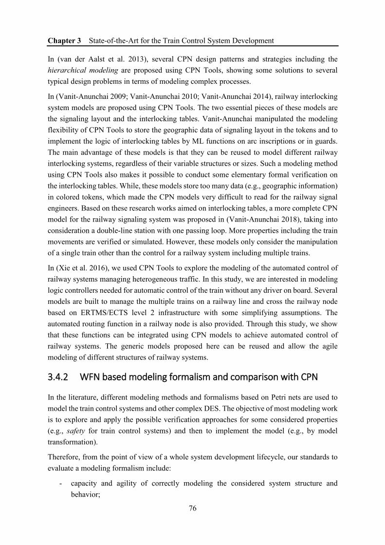
Chapter 3 State-of-the-Art for the Train Control System Development
76
In (van der Aalst et al. 2013), several CPN design patterns and strategies including the hierarchical modeling are proposed using CPN Tools, showing some solutions to several typical design problems in terms of modeling complex processes.
In (Vanit-Anunchai 2009; Vanit-Anunchai 2010; Vanit-Anunchai 2014), railway interlocking system models are proposed using CPN Tools. The two essential pieces of these models are the signaling layout and the interlocking tables. Vanit-Anunchai manipulated the modeling flexibility of CPN Tools to store the geographic data of signaling layout in the tokens and to implement the logic of interlocking tables by ML functions on arc inscriptions or in guards. The main advantage of these models is that they can be reused to model different railway interlocking systems, regardless of their variable structures or sizes. Such a modeling method using CPN Tools also makes it possible to conduct some elementary formal verification on the interlocking tables. While, these models store too many data (e.g., geographic information) in colored tokens, which made the CPN models very difficult to read for the railway signal engineers. Based on these research works aimed on interlocking tables, a more complete CPN model for the railway signaling system was proposed in (Vanit-Anunchai 2018), taking into consideration a double-line station with one passing loop. More properties including the train movements are verified or simulated. However, these models only consider the manipulation of a single train other than the control for a railway system including multiple trains.
In (Xie et al. 2016), we used CPN Tools to explore the modeling of the automated control of railway systems managing heterogeneous traffic. In this study, we are interested in modeling logic controllers needed for automatic control of the train without any driver on board. Several models are built to manage the multiple trains on a railway line and cross the railway node based on ERTMS/ECTS level 2 infrastructure with some simplifying assumptions. The automated routing function in a railway node is also provided. Through this study, we show that these functions can be integrated using CPN models to achieve automated control of railway systems. The generic models proposed here can be reused and allow the agile modeling of different structures of railway systems.
3.4.2 WFN based modeling formalism and comparison with CPN
In the literature, different modeling methods and formalisms based on Petri nets are used to model the train control systems and other complex DES. The objective of most modeling work is to explore and apply the possible verification approaches for some considered properties (e.g., safety for train control systems) and then to implement the model (e.g., by model transformation).
Therefore, from the point of view of a whole system development lifecycle, our standards to evaluate a modeling formalism include:
- capacity and agility of correctly modeling the considered system structure and behavior;

Chapter 3 State-of-the-Art for the Train Control System Development
77
- compatibility and facility with future system development phases, e.g., the possibility of verifying essential properties, the compatible model transformation method to generate the control code for implementation.
For a complex DES such as train control systems, high-level Petri nets are a good choice as they are provided with not only more compact representation, but also data manipulation. Among the different variants of high-level Petri nets, Colored Petri Nets (CPN) and Well-Formed Nets (WFN) as two common modeling approaches. They share the high-level Petri nets characteristics but have their own particularity.
Figure 3-6 compares the CPN and WFN approaches of modeling complex DES and the possible analysis methods applicable to their models.
Earlier in (Xie et al. 2016), we have modeled an entire train control system in CPN Tools and tried to analyze the CPN models of a railway control system using the different approaches, as shown in the left part of Figure 3-6.
Figure 3-6 Analyzability comparison of CPN and WFN
The most direct analysis method to analyze CPN models is to generate its reachability graph which enables to check the required properties. The way is always theoretically correct, however, the application of this method to such a large-scale railway control system encounters the famous combinatorial explosion problems and it can thus be used in very limited cases.
One possible way to combat this combinatorial explosion would be to reduce the initial CPN models before constructing the reachability graph. However, there are very little reduction rules applicable to CPNs and each of them has their own rigorous applicable constraints. For example, the reduction rules proposed in (Esparza and Hoffmann 2016) are only applicable to
Railway Requirement Specifications
Colored Petri Net Models (CPNs) Well-Formed Net Models(WFNs)
Reachability Graph
Unfolded PNs
Reduced WFNsReduced
PNs
Colored invariants
Symbolic Reachability Graph
Modelling
Model Transforming
Analysis and Verification
ReducedCPNs
P/T invariants
Reduction Unfolding
Reduction
Reduction

Chapter 3 State-of-the-Art for the Train Control System Development
78
certain structures in free choice workflow nets with the objective of maintaining the soundness property. This is probably a result of the high abstract degree and agility of CPN.
In order to make use of more general reduction rules, an available solution is to first go through an unfolding process of CPN to get the underlying ordinary PNs. Then it is possible to apply some existing reduction rules of ordinary PNs (Berthelot and Lri-Iie 1986; Murata 1989). This approach seems to be a good idea but in practice, it is always blocked when it comes to complex and large-scale DES, e.g. train control system, because one is often confronted with a combinatorial explosion problem in the unfolding operation.
It is also worth noting that some extensions of colored Petri nets are integrated with different kinds of techniques to further enhance its expressivity (e.g., the use of ML – Meta-Language – in CPN Tools). The use of these extensions always results in a loss of eligibility to apply the reduction and analysis methods and makes it more difficult to unfold the nets as not all the methods are compatible with the extensions.
Essentially, the problematic situation is a compromise between the modeling power of the selected modeling approaches and the possibility of making formal verification.
To deal with this problem, some colored Petri nets with constraints are proposed, among which the Well-formed Petri Nets (WFN) are of interest to us. WFN have some syntactical constraints as shown in its name and some good features which facilitate its analysis. It is also pointed out in (Haddad et al. 1995) that WFNs have the same expressive power as general CPN (Jensen 1982) despite a very rigorous syntax.
The right part of Figure 3-6 describes the possible analysis approaches applicable to WFN models. To avoid the combinatorial explosion, several reduction rules could first be applied. As WFN are Petri nets abbreviations and can always be unfolded to ordinary Petri nets, the Colored nets reduction theory based on folding proposed in (Haddad 1991) can also be applied. With regard to the state space analysis, the symbolic reachability graph will greatly reduce the size of the reachability graph for the models including symmetries.
As the objective of this thesis is to propose appropriate Petri Net patterns whose properties can be checked before the models are implemented, we have chosen to use WFN as modeling formalism for modeling autonomous railway control systems, in order to benefit from the advantages of analyzing a WFN model.
3.5 Conclusion of Chapter 3
This chapter introduces the theoretical framework of the thesis.
First, we review lots of common system development approaches that can be used for the train control system design. We conclude that Petri nets are an ideal formalism.

Chapter 3 State-of-the-Art for the Train Control System Development
79
Then, we review the Petri nets theory and discuss different Petri net variants. Taking into consideration the complexity of train control systems, we prefer to use high-level Petri nets as they have a more compact expression. Two formalisms – colored Petri nets (CPN) and well-formed Petri nets (WFN) – are used in this thesis for the reason of abundant extensions and the facility of analysis, respectively. We introduced these two formalisms and the software for them, e.g., CPN Tools.
At the end of this chapter, a literature review of modeling methods and practice with these two Petri net formalisms are given. We also compare the advantages and inconvenient of them.


81
Chapter 4 MODULAR MODELING FOR TRAIN CONTROL SYSTEMS
4.1 Introduction to Chapter 4
Train control systems are large-scale and complex Discrete Event Systems (DES). In order to model the train control systems in an efficient way, this chapter introduces a modeling methodology containing different modular modeling methods and techniques.
§4.2 introduces our modular modeling methodology as a whole. Faced with such a complex train control system, our methodology considers both a structural decomposition and a functional decomposition to reduce the complexity. Then, the two kinds of decomposition are integrated by conducting a mapping between them to an abstracted system model faced with a certain modeling objective. The abstracted system model contains different structural components and functions. Following this approach, an abstracted system model is constructed and is used as the global railway model in this chapter.
§4.3 introduces the structural modeling of a railway control system. The global railway system is modeled by different components and their interfaces. Each type of component is modeled as a generic module in colored Petri nets and can be reused by its different instances. Two different methods to implement the reusability are compared. Different modeling methods of interfaces are also proposed to implement the communications and information exchange within or between the component models.
In the rest of this chapter, we introduce the modeling methods for the three main components in a railway control system: the ETCS onboard system (train), the RBC and the railway node controller. The concrete modeling of each component is developed from a functional viewpoint.
§4.4 concentrates on the functional modeling ETCS onboard system, which may be the most sophisticated component in the global abstracted model. In order to further reduce the modeling complexity, we propose to use the functional modeling approach within the scope of the onboard system. The onboard system behavior is analyzed, and three levels of functionality are modeled by mode (transition), procedure, and onboard function, with respect to the ETCS system requirements specification.
The automatization of a train control depends on the interaction and cooperation of both the onboard system and the trackside system. That is why we introduce the modeling of railway

Chapter 4 Modular Modeling for Train Control Systems
82
node component with automated routing function in §4.5, and the modeling of the RBC component with the Movement Authority (MA) function in §4.6.
In order to illustrate the advantages and the drawbacks of different formalisms, the train component and railway node component are modeled using colored Petri nets with CPN Tools, while the RBC component is modeled with well-formed Petri nets (WFN) with the expectation to benefit from its favorable compatibility with different analysis techniques. However, the constraints of modeling in WFN could be an obstacle to model some sophisticated behaviors of the RBC component. Thus, we propose three general modeling patterns to enhance the modeling expressivity of WFN. It is worth noting that these patterns are general techniques that can be applied to the modeling of a similar system in WFN.
§4.7 concludes this chapter.
4.2 Modular Modeling Methodology of Train Control Systems
Faced with the modeling task of a complex DES, the modular design based on decomposition is usually an intuitive choice for the modelers as well as for the domain experts to fight against the system complexity.
The decomposition of a global system can be achieved by the following two approaches:
• Structural decomposition in reference to the real system architecture;
• Functional decomposition of the global system or subsystems.
In order to facilitate the modeling of the complex system, we decompose the system in both a structural way and a functional way by applying a top-down approach, as shown in Figure 4-1. Then, we conduct a mapping process of the structural decomposition and functional decomposition to obtain an abstracted system model.
Figure 4-1 Train control system modeling methodology
The modular design has many advantages. The modularity implies the reusability of the system modules. The modular modeling methods can also facilitate modular verification by using the same system architecture, which provides efficient and flexible analysis techniques (Christensen and Petrucci 2000). In the field of manufacturing systems, the modular design
Functional decomposition
Structural decomposition
Abstracted system model
Mapping the structural and functional decompositions

Chapter 4 Modular Modeling for Train Control Systems
83
allows a distributed workshop, which can facilitate the dynamic reconfiguration of flexible production lines (Da Silveira et al. 2002).
Some Petri nets formalisms, e.g., hierarchical colored Petri nets (Jensen 1992), can offer the support for a modular design approach.
4.2.1 Structural Decomposition
The practical railway control system is very large, complex and distributed system with thousands of components deployed in different places. In order to be able to model such a system, a structural decomposition is necessary. Figure 4-2 follows a top-down approach based on structural modularity to decompose the whole railway control system.
In this structural decomposition, most of the components are reusable and may be found of multiple duplicates in a decomposition. For example, there may be several RBCs for a railway line. Different higher-level components may also use the same lower-level component. For example, the track circuit is used as a train detection device both in the blocks of a railway line and in the railway stations or nodes as parts of the interlocking system.
Figure 4-2 Structural decomposition of the railway control system
4.2.2 Functional Decomposition
There are many functions in a railway control system. In order to better identify and analyze the functions, we use a top-down hierarchical functional decomposition to represent the major functions in a modern train control system, as shown in Figure 4-3.
Different levels can be found in the functional decomposition. A macro-function, which is presented by rounded-corner rectangles with a bold border, can be decomposed to several sub-functions, which are presented by simple rounded-corner rectangles. For example, the macro-function “Movement Authority (MA) Management” can be decomposed to the sub-functions “MA request, generation and update”, “RBC handover” and “Emergency stop”. Each sub-function can be further realized by concrete functions, which are represented by shadowed rounded-corner rectangles in Figure 4-3.
Railway control system(Structural decomposition)
Infrastructure Onboard
Railway line
Railway station(or railway node)
CTC Block signalingRBCStation signaling
Eurobalise(station)
Track circuit(station)
Switch(station)
Eurobalise(block)
Track circuit(block)
Switch(block)
ETCS onboard equipment
TIU DMI BTM EuroradioEVC

Chapter 4 Modular Modeling for Train Control Systems
84
Figure 4-3 Functional decomposition of a railway control system
The concrete functions often reflect the specific articles in the system requirements specification. These concrete functions need to be implemented by relevant hardware or software system. In Figure 4-3, the concrete functions can be found in the system requirements specification (SRS) of ERTMS/ETCS (European Railway Agency 2016a). The dotted lines with the tag <ref> connect the concrete functions to the text references in SRS. Later in this chapter, we will further introduce how to model these concrete functions in CPN Tools.
4.2.3 Mapping the Structural and Functional Decompositions
The structural and functional decompositions show the way that a whole railway control system is composed of many components and has numerous functions. These components and functions are intertwined with each other. Thus, the modeling of the whole railway control system is difficult but, in most cases, unnecessary. We propose a modeling methodology which allows the modelers to form abstracted and representative models according to their different modeling objectives. The abstracted models are obtained by mapping the structural and functional decompositions together.
In practice, a modeling objective can be expressed by several items in the functional decompositions (i.e., macro-functions, sub-functions or concrete functions). These functions are associated with the necessary components from the structural decompositions.
For example, an important operational scene in ERTMS/ETCS level-2 is the management of multiple trains in the railway lines based on Movement Authorities (MA, permission for a
Railway Control System(Functional Decomposition)
Position / Speed Management
MA Management
Train Speed Supervision
Speed Profile Determination
Speed monitoring and intervention
Special movements supervision
Traffic control and dispatching
Position detection
Speed and acceleration detection
Position request and report
MA request, generation and update
RBC handover
Emergency stop
Temporary Speed Restrictions (TSR)
Override and trip management
Station (node) pass-through
Onboard requests MA Cyclicallyrespect to location approach or timerelapsing (level 2/3)
Onboard requests MA Cyclicallywhen “Start” is selected (level 2/3)
Determination of EoA (End ofauthority), danger point, etc.
···
SRS 3.8.2.3 a);SRS 3.8.2.3 b)
SRS 4.4.11;SRS 5.4;SRS 5.11
SRS 3.8.4;SRS 3.8.5
<ref>
<ref>
<ref>
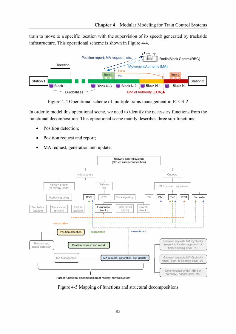
Chapter 4 Modular Modeling for Train Control Systems
85
train to move to a specific location with the supervision of its speed) generated by trackside infrastructure. This operational scheme is shown in Figure 4-4.
Figure 4-4 Operational scheme of multiple trains management in ETCS-2
In order to model this operational scene, we need to identify the necessary functions from the functional decomposition. This operational scene mainly describes three sub-functions:
• Position detection;
• Position request and report;
• MA request, generation and update.
Figure 4-5 Mapping of functions and structural decompositions
Train 2Train 1
End of Authority (EOA)
Block NBlock N-1Block N-2
Movement Authority (MA)Direction
Radio Block Centre (RBC)Position report, MA request., etc.
Eurobalises
Speed
Station 2Station 1Block 1 Block N-3
MA
Railway control system(Structural cecomposition)
Infrastructure Onboard
Railway line
Railway station(or railway node)
CTC Block signalingRBCStation signaling
Eurobalise(station)
Track circuit(station)
Switch(station)
Eurobalise(block)
Track circuit(block)
Switch(block)
ETCS onboard equipment
TIU DMI BTM EuroradioEVC
Position request and reportPosition and speed detection
<associate>
MA Management MA request, generation and update
Onboard requests MA Cyclically respect to location approach or
timer elapsing (level 2/3)
Onboard requests MA Cyclically when “Start” is selected (level 2/3)
Determination of EoA (End of authority), danger point, etc.
<associate>
Part of functional decomposition of railway control system
Position detection <associate>

Chapter 4 Modular Modeling for Train Control Systems
86
The implementation of these functions relies on relevant components. A function may be associated with a single component or different components which are even across the infrastructure and the onboard system.
According to different modeling objective, the mapping can be actualized by considering the different depths in the structural and functional decomposition.
Figure 4-5 shows the mapping of three sub-functions and the structural decomposition. A dotted line with <associate> tag associates a function to its relevant components. Our method is to choose the appropriate components and to build their connections according to the concerned functions to finally create the abstracted model.
4.2.4 Specification of Abstracted System Model
4.2.4.1 Example of an abstracted system model
The idea of building an abstracted system model is based on the fact that a railway control system is too large to be analyzed in its full size and too complex to be modeled with all the components in detail.
The aforementioned structural decomposition, functional decomposition and the mapping between them show how the different parts are coupled to construct the global system. Based on the decompositional analysis and the practical modeling objective, we can finally build an abstract system model of a reduced size by identifying the principal train control functions in question and by modeling only the necessary components as well as the connection between them with regard to these functions.
This study aims to contribute to the feasibility of autonomous trains in the context of ERTMS/ETCS. It needs the cooperation of the onboard system and the trackside components.
The modeling objective of the abstracted system model is to allow a passthrough of a train in the railway system with a certain degree of automation. We consider the following functions shown in Table 4-1.
Table 4-1 Principal train control functions in the abstracted model
Traffic management in railway lines Railway node (station) automation
Onboard Speed supervision and control with
respect to movement authority (MA) Passing the railway node (station)
along the assigned routes.
Trackside MA generation (in RBC) according to
the traffic in railway lines Automated route selection and
interlocking
Considering these functions listed in Table 4-1, the following components concerned will be modeled in the abstracted system model:

Chapter 4 Modular Modeling for Train Control Systems
87
• Onboard (Train):
o EVC
o BTM (modeled as an external interface)
o Euroradio (modeled as an external interface)
o DMI (modeled as an external interface)
• Trackside:
o Railway line:
RBC
Eurobalise (to offer the balise telegrams)
o Railway node or railway station:
Track circuit
Switch
Signal machine
For the trackside components, the relationship between the different components in practice could be very different depending on the railway network architecture. In this chapter, we use a simple but representative railway system structure illustrated in Figure 4-6 to build the abstract system model. This structure also has a good coherence with the layout of the railway node previously presented in Figure 2-1.
Figure 4-6 Railway system structure for the abstract model
The considered trackside components are:
- Four stations (Stations A, B, C and D) and a railway node (Node N);
- Four railway lines connecting these stations and the node, where all the trains considered are in the same direction;
- RBC 1 and RBC 2, which manage the railway line from Station A to Node N, and that from Node N to Station C, respectively.
A C
B D
Node N
Station A
Station DStation B
Station C
RBC 1 controlled area RBC 2 controlled area
Direction
Chapter 4 Modular Modeling for Train Control Systems
88
4.2.4.2 Modeling assumptions of the abstract system model
Our modeling methods to be proposed respect the actual ERTMS/ETCS system requirements specification (European Railway Agency 2016a). However, a set of simplifying assumptions are also considered to reduce the complexity of the models so that they could be represented in a thesis. We believe that these assumptions do not affect the presentation of our modeling methodology.
The principal simplifying assumptions are shown as follows:
1. Train length is not taken into account for simplification reasons. Thanks to this assumption, we can use a single position to represent several different position-based concepts, e.g., “min safe train front end” and “max safe train front end” are merged.
2. A railway line is considered to have a fixed operation direction and trains on a railway line cannot overtake (by using passing siding rails). This assumption results in a non-exchangeable order of the trains on a railway line.
3. A single RBC manages all the trains on the same railway line. In other words, the “RBC handover” function is not supported.
4. Movement Authority (MA) is simplified to only one section and some optional timer parameters are also ignored. In an MA message, only the EOA (End of Authority) position is in our interest.
5. Since the modeling method is DES-oriented and the modeling objective is the general behavior of the whole railway system, i.e., the control of multiples trains other than a standalone onboard system, some details of continuous concepts, e.g., train speed, braking performance, the train’s exact position in a block section, are simplified. As a consequence, we assume that a train can always stop before the end of the current block it occupies.
4.3 Structural Modeling of Train Control System
4.3.1 Introduction to Structural Modeling
This study proposes a structural modeling method based on colored Petri nets to model complex systems, taking train control system as an example. This method focuses on the modeling of a global railway system. It takes advantage of the structural decomposition to model each type of physical component as a reusable component module. Then the instances of these components are connected together according to their relationship to obtain a global system model.
In this section, we propose to model each kind of structural component (e.g., train, RBC, railway node) by a generic module using colored Petri net. Such a generic module is reusable

Chapter 4 Modular Modeling for Train Control Systems
89
by all its instances. The major difficulties are to distinguish different instances of the same module and to deal with the connection and communication between different modules or their instances.
Faced with these difficulties, we introduce two techniques of component modeling to achieve the reusability: the parametric module representation and the structured token representation. The former exploits the hierarchical support in CPN Tools via the substitution transition, while the latter takes advantage of the compound structure of colored token. The two techniques allow the existence of multiple instances in a global system model by building only one generic module. We compare the two approaches and explain our preference to the parametric module representation, which contributes to an intuitive and structural representation of the global system model.
We also introduce several modeling methods of interfaces and communication techniques between different modules and their instances, according to different modeling objectives. These interface modeling methods, together with the component modeling methods, allow the construction of a global system model.
The examples of the implementation of the structural modeling method will be represented with CPN Tools.
4.3.2 Component Modeling
A generic component module is defined as a reusable modeling brick and can have multiple instances in a global system. The reusability can be achieved in different ways. We propose two modeling techniques to represent the multiple instances of the same component by reusing a generic component module: the parametric module representation and the structured token representation.
4.3.2.1 Parametric module representation
The parametric module representation defines a general modeling form of a system component by a CPN parametric module with the following parts:
• Module body;
• Parameter place(s);
• Interface place(s).
Figure 4-7 shows three instances of two different modules modeling using the parametric module representation. The rectangles named with “Module X (instance Y)” represent the module body. The white ellipses named with “P X.Y.N” shows the Nrd parameter place of the instance Y of module X. The colored ellipses represent the interface between different instances of the same module or those between different modules.
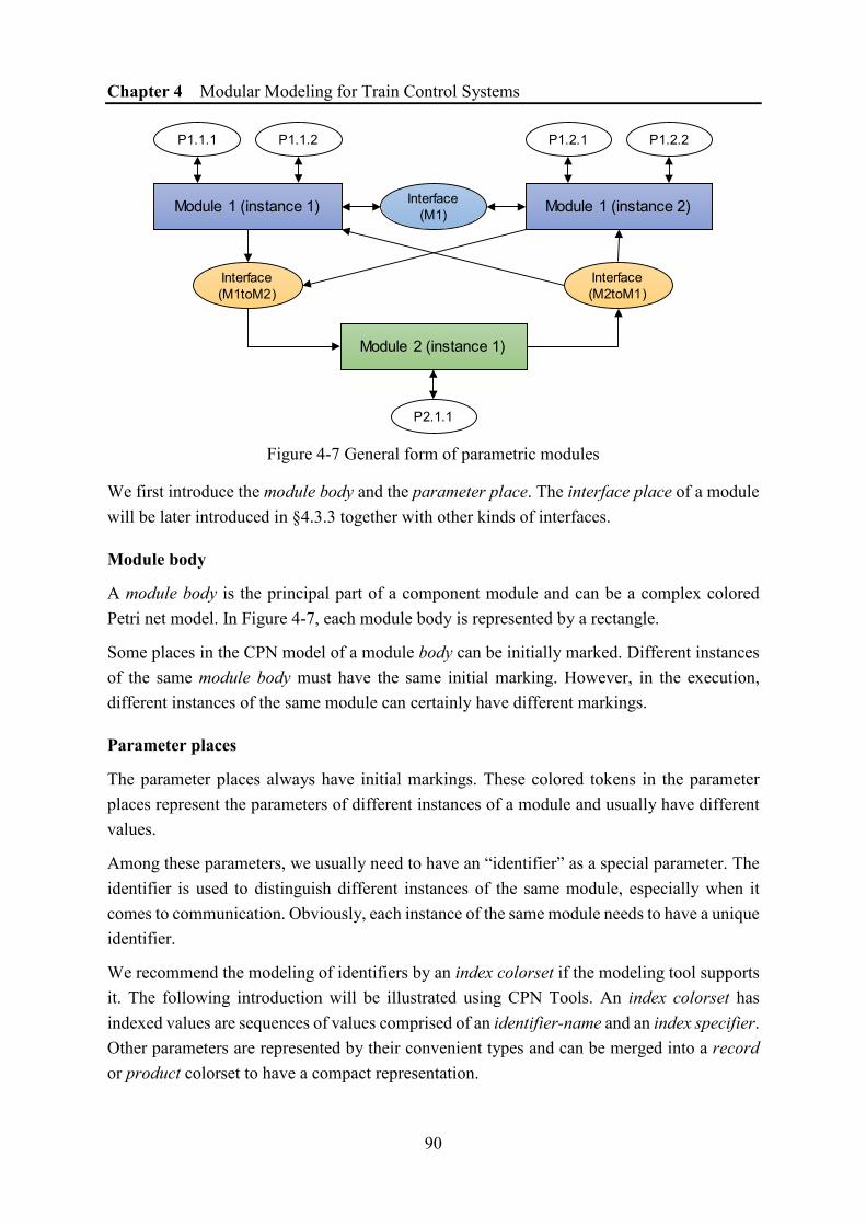
Chapter 4 Modular Modeling for Train Control Systems
90
Figure 4-7 General form of parametric modules
We first introduce the module body and the parameter place. The interface place of a module will be later introduced in §4.3.3 together with other kinds of interfaces.
Module body
A module body is the principal part of a component module and can be a complex colored Petri net model. In Figure 4-7, each module body is represented by a rectangle.
Some places in the CPN model of a module body can be initially marked. Different instances of the same module body must have the same initial marking. However, in the execution, different instances of the same module can certainly have different markings.
Parameter places
The parameter places always have initial markings. These colored tokens in the parameter places represent the parameters of different instances of a module and usually have different values.
Among these parameters, we usually need to have an “identifier” as a special parameter. The identifier is used to distinguish different instances of the same module, especially when it comes to communication. Obviously, each instance of the same module needs to have a unique identifier.
We recommend the modeling of identifiers by an index colorset if the modeling tool supports it. The following introduction will be illustrated using CPN Tools. An index colorset has indexed values are sequences of values comprised of an identifier-name and an index specifier. Other parameters are represented by their convenient types and can be merged into a record or product colorset to have a compact representation.
Module 1 (instance 1)
P1.1.1
Module 1 (instance 2)
Module 2 (instance 1)
P1.1.2
Interface (M1)
P1.2.1 P1.2.2
Interface (M1toM2)
Interface (M2toM1)
P2.1.1

Chapter 4 Modular Modeling for Train Control Systems
91
Code 4-1 shows an example of the declaration of the parameters of a train component. Among these parameters, colorset TRAINNO is defined as an index colorset and is used as an identifier. The examples of its values could be Train (1), Train (2), …, Train (10). A record colorset TrainAttribute assigns other parameters to an instance of the train component, such as train type, train mass, its origin and destination stations.
Code 4-1 Declarations for parameter places of component train (part of) 1 (*Declaration for parameter places of component train*) 2 colset TRAINNO = index Train with 0..10; 3 var tno: TRAINNO; 4 colset TrainType = with Passenger | freight; 5 colset TrainMass = int with 0..100000; 6 colset StationName = string; 7 colset TrainAttribute = record tType:TrainType *
tMass:TrainMass * tOrigin:StationName * tDesti:StationName;
In Petri net models, a parameter place is usually linked to its module body via a bi-directional arc as shown by the example in Figure 4-8. The bi-directional arc implies that a parameter place can be accessed by the component model but will always maintain their values throughout the execution. In other words, a parameter place is usually read-only for the module body.
Figure 4-8 Example of parameter places of train component
Reusability of a parametric module
The component model offers the modeling bricks and can be reused. The parametric module representation exploits the hierarchy support in CPN Tools to represent different instances in a global model of the railway system.
The parametric module representation proposes to model the instances of components in two layers: the global layer (higher level) and the (lower) component layer (lower level).
The global layer mainly defines the configuration of the instances of the components and illustrates the connections between them, as shown in Figure 4-7. This global layer is also modeled as a colored Petri net model. In CPN Tools, the module body of each instance is represented by a substitution transition (rectangles with double-line borders in Figure 4-8) in this global layer. The use of substitution transition has double advantages:

Chapter 4 Modular Modeling for Train Control Systems
92
• For the modeling, the detailed structure of the module body in the global layer is hidden, which allows a simplified broad overview of each instance to help the modelers concentrate on their relationship;
• For the execution, the underlying component instance model for each substitution transition can be executed independently by the support of CPN Tools.
As an example, let us consider the global model of a simple case study. Following the decomposition of §4.2.1, we abstract the railway control system as composed of ETCS onboard system (train hereafter for simplicity), RBCs and controllers of railway node (node hereafter for simplicity). Based on the structure of the abstracted system presented in Figure 4-6, two instances of the component Train (Train 1 and Train 2), two instances of component RBC (RBC 1 and RBC 2) and an instance of railway node (Node N) are modeled in Figure 4-9 using the parametric module representation.
In the global layer, each instance is modeled as a substitution transition and is parametrized by its parameter place. The two instances of the train module are modeled by the substitution transitions noted respectively Train1 and Train2. Each of these transitions is linked to its parameter place noted T1info (for Train1) and T2info (for Train2) by bi-directional arcs. In order to have a more compact representation, we use a unique parameter place with a compound colored token in a form of (4-1) to represent both the train identifier and the
necessary train attributes.
(Identifier, Attribute 1, Attribute 2, … , Attribute n) (4-1)
In the same way, the two instances of the RBC component are also modeled by substitution transitions noted respectively RBC1 and RBC2, together with the parameter places RBCinfo1 and RBCinfo2. The instance nodeN has a parameter place NodeName which is used to store its identifier.
The interface places enable to model the communication from one type of components to another type of components. For example, in Figure 4-9 the place Train2RBC models the communications from the train instances to the RBC instances and in the example is not possible for RBCs and the node N to communicate directly. The structure of colored tokens put in the interface places enables to define the concrete participants of the communication, which will be later introduced in §4.3.3.
The global layer model can be easily modified by connecting/disconnecting components to the corresponding interfaces.
As to the component layer, it defines a concrete model for each type of component. We will later introduce the modeling method for the train, RBC and node component module

Chapter 4 Modular Modeling for Train Control Systems
93
respectively in §4.4–4.6§. With the support of CPN Tools hierarchy, each instance of component module behind a substitution transition can be executed independently.
Figure 4-9 An example of modeling by parametric module representation
4.3.2.2 Structured token representation
An alternative technique of reusing a component module to represent its different instances is also possible. Instead of using the hierarchical support in CPN Tools, this technique takes advantage of the flexibility of colored token in colored Petri nets.
It represents each instance of the same component by a structured colored token, which contains the identifier, the parameters and possibly some necessary execution states. The structured token representation models the whole system in a flat structure without explicit hierarchy. In the system model, each component module has only one presence regardless of the number of its instances. The different instances of the same component module are thus represented by different structured colored tokens in the places of the component module. In order to distinguish the behavior of different instances in the single model, it is obliged to assign an identifier for each instance and to include the identifier filed in each colorset of the component model. The structured token can be implemented by some compound types, such as the color domain in WFN, and the product colorset or record colorset in CPN Tools.
Figure 4-10 compares a part of the train component model implemented with parametric module representation via CPN Tools hierarchy (a) and the corresponding model implemented with structure token representation via product colorset (b).
The differences can be found in the following aspects:
(1) A neutral colorset (colorset “UNIT”) in (a) is modeled as the identifier’s colorset “TRAINNO” in (b);
(2) A product colorset “A x B x … x C” is modeled as “TRAINNO x A x B x … x C” in (b);

Chapter 4 Modular Modeling for Train Control Systems
94
(3) Any other colorset “COL” excluding neutral/product in (a) is modeled as a product colorset “TRAINNO x COL” in (b);
(4) For any expression in (a) without a variable of colorset “TRAINNO”, it is modeled by a corresponding expression with a variable of colorset “TRAINNO” (variable “tno” in the example);
(5) The parameter place only to assign an identifier in (a) is no longer necessary in (b) as the identifier is repeated in every place.
Figure 4-10 Comparison of two methods to model a component module
In Table 4-2, the characteristics of the two representation methods are further compared.
Table 4-2 Comparison of two reusability methods for component models
Representation Parametric module Structured token
Modeling tool support CPN Tools hierarchy Colored Petri nets
Model readability Good Middle
Dynamic feature (Add/remove instances)
Difficult Middle
Global state space Same orders-of-magnitude
By using the structured token representation, the global model may be more compact compared to the parametric module representation, but less readable because the system structure is not explicitly represented.
An advantage of the structured token representation could also be the possibility of adding and removing instances by manipulating the tokens. These operations could be more difficult
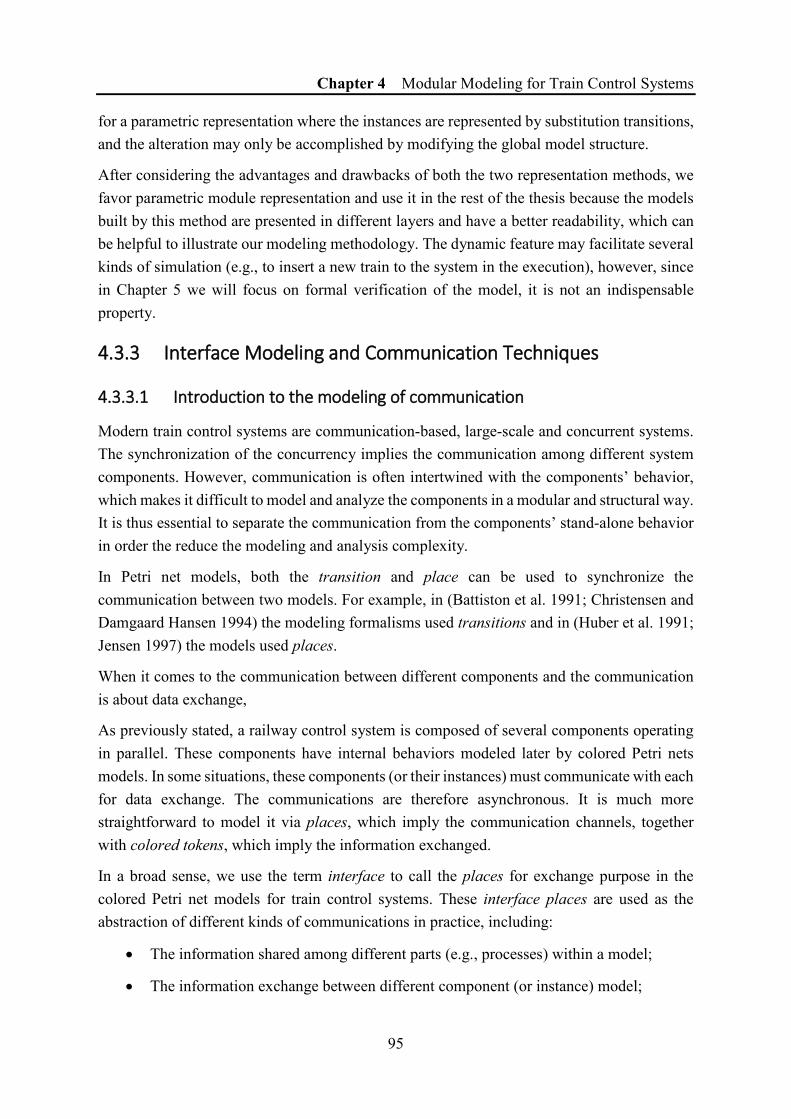
Chapter 4 Modular Modeling for Train Control Systems
95
for a parametric representation where the instances are represented by substitution transitions, and the alteration may only be accomplished by modifying the global model structure.
After considering the advantages and drawbacks of both the two representation methods, we favor parametric module representation and use it in the rest of the thesis because the models built by this method are presented in different layers and have a better readability, which can be helpful to illustrate our modeling methodology. The dynamic feature may facilitate several kinds of simulation (e.g., to insert a new train to the system in the execution), however, since in Chapter 5 we will focus on formal verification of the model, it is not an indispensable property.
4.3.3 Interface Modeling and Communication Techniques
4.3.3.1 Introduction to the modeling of communication
Modern train control systems are communication-based, large-scale and concurrent systems. The synchronization of the concurrency implies the communication among different system components. However, communication is often intertwined with the components’ behavior, which makes it difficult to model and analyze the components in a modular and structural way. It is thus essential to separate the communication from the components’ stand-alone behavior in order the reduce the modeling and analysis complexity.
In Petri net models, both the transition and place can be used to synchronize the communication between two models. For example, in (Battiston et al. 1991; Christensen and Damgaard Hansen 1994) the modeling formalisms used transitions and in (Huber et al. 1991; Jensen 1997) the models used places.
When it comes to the communication between different components and the communication is about data exchange,
As previously stated, a railway control system is composed of several components operating in parallel. These components have internal behaviors modeled later by colored Petri nets models. In some situations, these components (or their instances) must communicate with each for data exchange. The communications are therefore asynchronous. It is much more straightforward to model it via places, which imply the communication channels, together with colored tokens, which imply the information exchanged.
In a broad sense, we use the term interface to call the places for exchange purpose in the colored Petri net models for train control systems. These interface places are used as the abstraction of different kinds of communications in practice, including:
• The information shared among different parts (e.g., processes) within a model;
• The information exchange between different component (or instance) model;

Chapter 4 Modular Modeling for Train Control Systems
96
• The extra information between the considered system and its environment, which is usually used for simulation or verification purpose (e.g. the sequence of drive operations).
From a point of view of the modeling formalism in colored Petri nets using CPN Tools, we propose three different modeling methods of interfaces for different purposes and practical requirements.
4.3.3.2 Modeling of Interface by CPN Tools hierarchy
The hierarchical feature supported in CPN Tools offers a possibility of implementing the interfaces between different component models or their instances.
Figure 4-11 shows an example system modeled with two layers: the global layer and the component layer. Two components “Train” and “RBC” are modeled using the component modeling method of the parametric module representation. In the example, one instance of each component is used to build a global model. Transitions “Train” and “RBC” are substitution transitions in CPN Tools and their details are modeled in the module body of the corresponding component modules. Places “Train1” and “RBC1” are parameter places where are used to assign different identifiers and parameters to different instances of the same component. Place “T2RBC” is an interface place which is used to transform information from a train instance model to an RBC instance model.
Figure 4-11 Modeling of interfaces by CPN Tools hierarchy
An interface modeled by CPN hierarchy is implemented by port/socket assignments, which are used to equate places on the two layers. Such a place on the lower layer (component layer) is called a port, and that on the higher layer (global layer) is called a socket.
A port is always associated with a port-type tag (the blue tags in Figure 4-11) and can be one of the three kinds according to the direction: tag “In” for “input”; tag “Out” for “output” and tag “In/Out” for both the two directions.
RBC
global layer
Component layer ( CPN Tools subnets)
T2RBCTrainTrain1 RBC1
Train Module Body RBC Module Body
Out In
In/Out In/Out

Chapter 4 Modular Modeling for Train Control Systems
97
A socket is an input place or an output place of a substitution transition, i.e. there is always at least one arc between a substitution transition and a socket.
By using the port/socket assignments, a component module can be “glued together” with the surroundings of its corresponding substitution transition. Each socket must be assigned to a port on the corresponding subpage. A port with a tag “In” must be assigned to a socket which is an input place of the substitution transition. Analogously, an “Out” port requires a socket which is used an output place of the substitution transition.
While, a port with tag “In/Out” indicates that the socket must be both an input place and output place (other than “either of them”). In the example, the “In/Out” ports are used by the parameter places because that the identifiers and parameters in these places are normally to be referred to, other than to be generated nor to be consumed.
An interface place is a socket place with multiple port/socket assignments (i.e., multiple ports from different components or instances are assigned to the interface place). In the example, the interface place “T2RBC” is a socket on the global layer. Both an “Out” port from the train module and an “In” port from the RBC component are assigned to it. By this method, all the three places are somehow equated. By this method, the information can be transferred between different components or instances. Specifically, in the example of Figure 4-11, the train component model sends a piece of information to the RBC by generation a token in its port with an “Out” tag. This token ascends to the interface place “T2RBC” on the global layer owe to a port/socket assignment between the global model and the train module. Another port/socket assignment between the global model and the RBC component allows the RBC component to obtain this token from the interface place “T2RBC”, which models the reception of the information sent by the train.
In our modeling methodology, an interface implemented by CPN Tools hierarchy is mainly used to model the mono-directional communication between two components or their instances, i.e., from a component of type i to a component of type j. Bidirectional communications between two types of components can be modeled by using a pair of interfaces.
In this context, A particular interface is modeled on the global layer to transfer information from a certain type of component (sender) to a certain type of component (receiver). In the example shown in Figure 4-7, three interfaces places are defined for:
• Information exchange from an instance of component Module 1 to an instance of Module 2;
• Information exchange from an instance of component Module 2 to an instance of Module 1;
• Information exchange between different instances of Module 1.
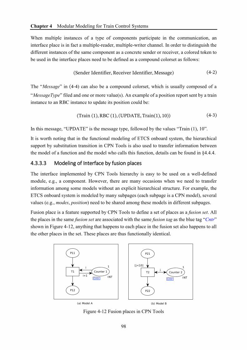
Chapter 4 Modular Modeling for Train Control Systems
98
When multiple instances of a type of components participate in the communication, an interface place is in fact a multiple-reader, multiple-writer channel. In order to distinguish the different instances of the same component as a concrete sender or receiver, a colored token to be used in the interface places need to be defined as a compound colorset as follows:
(Sender Identifier, Receiver Identifier, Message) (4-2)
The “Message” in (4-4) can also be a compound colorset, which is usually composed of a
“MessageType” filed and one or more value(s). An example of a position report sent by a train instance to an RBC instance to update its position could be:
(Train (1), RBC (1), (UPDATE, Train(1), 10)) (4-3)
In this message, “UPDATE” is the message type, followed by the values “Train (1), 10”.
It is worth noting that in the functional modeling of ETCS onboard system, the hierarchical support by substitution transition in CPN Tools is also used to transfer information between the model of a function and the model who calls this function, details can be found in §4.4.4.
4.3.3.3 Modeling of Interface by fusion places
The interface implemented by CPN Tools hierarchy is easy to be used on a well-defined module, e.g., a component. However, there are many occasions when we need to transfer information among some models without an explicit hierarchical structure. For example, the ETCS onboard system is modeled by many subpages (each subpage is a CPN model), several values (e.g., modes, position) need to be shared among these models in different subpages.
Fusion place is a feature supported by CPN Tools to define a set of places as a fusion set. All the places in the same fusion set are associated with the same fusion tag as the blue tag “Cntr” shown in Figure 4-12, anything that happens to each place in the fusion set also happens to all the other places in the set. These places are thus functionally identical.
Figure 4-12 Fusion places in CPN Tools

Chapter 4 Modular Modeling for Train Control Systems
99
The members of a fusion set can be from almost anywhere. Several common cases are as follows:
- If all the places are on the same page, we could, in fact, replace the fusion set with a single place and connect to it all the arcs that are previously connected to any place of the fusion set. It helps to improve the modeling in terms of aesthetics and readability. An example can be found in Figure B-1 with the fusion set “CurrentMode”.
- The places of a fusion set could also be from different pages. A page is used as a container in CPN Tools where a CPN model is built. A complex model is usually separated into different pages thus each page could have a particular modeling objective. In this case, the fusion places are in fact connectors of different pages.
- The fusion places can be used together with a hierarchical model and a fusion set can contain members from models of different layers. In fact, the port/socket pair of the CPN Tools hierarchy is implemented by a special fusion set whose members are limited to the port/socket assignments. However, fusion places offer a more general approach to share the tokens from any places, which allows a communication method throughout all the global model.
One should be careful to use the fusion places with a hierarchical model with multiple component instances. In fact, the fusion set works like a global variable in the programming language. Any part of the model can access it and modify it. If a fusion place is used in the component module, the corresponding places in different component instants are always in the same fusion set and cannot have different markings.
4.3.3.4 Modeling of Interface via the file system
We have introduced two methods of modeling the interfaces for different objectives in CPN Tools. The two methods can cover the most requirements to model the interfaces in the scope of a CPN Tools net (i.e., a CPN Tools project).
However, for a very large-scale and complex system, the analysis or simulation of such a system may be distributed to different modeling projects implemented by different computers. In this situation, even the CPN Tools does not offer native support to connect the two models.
We propose a universal solution to make the connection between two models by establishing an interface via the file system. Thus, the different entities using this interface could be in the same model, in different models on the same computer, or even on different computers as long as they can access the storage where stores the interface file. This method is also useful to implement the communication between different kinds of models using different modeling tools (e.g., a CPN Tools model and a WFN model) as long as the modeling tools offer the conversion method between file stream and multiset.

Chapter 4 Modular Modeling for Train Control Systems
100
Figure 4-13 Interfaces via file sharing
Figure 4-13 shows an illustrative example of interface modeling via the file system. We consider the transmission of the position report from a train instance to an RBC instance. The example is like that of Figure 4-11, however, by using the interface via the file system, the two-component model (i.e., train model and RBC model) can be on different computers.
The position report message to be transmitted is modeled using the format (𝑆𝑆𝑇𝑇𝑇𝑇𝑆𝑆𝑇𝑇𝑉𝑉 𝐼𝐼𝑆𝑆𝑇𝑇𝑇𝑇𝑡𝑡𝑇𝑇𝐼𝐼𝑇𝑇𝑇𝑇𝑉𝑉, 𝐸𝐸𝑇𝑇𝑐𝑐𝑇𝑇𝑇𝑇𝑣𝑣𝑇𝑇𝑉𝑉 𝐼𝐼𝑆𝑆𝑇𝑇𝑇𝑇𝑡𝑡𝑇𝑇𝐼𝐼𝑇𝑇𝑇𝑇𝑉𝑉, 𝑀𝑀𝑇𝑇𝑠𝑠𝑠𝑠𝑎𝑎𝑀𝑀𝑇𝑇), and the Message filed is simplified to a position value. Part of the definition of colorsets and variables used in the example can be found in Code 4-2.
Code 4-2 Declaration for example of interface via file system
1 colset TRAIN = index T with 1..10; 2 colset RBC = index RBC with 1..10; 3 colset POS = int with ~1..1000000; 4 colset TxRBCxPOS = product TRAIN * RBC * POS; 5 colset TRAINxPOS= product TRAIN * POS; 6 var msg: TxRBCxPOS; 7 var tr: TRAIN; 8 var rbc: RBC; 9 var pos: POS; 10 var i, j:INT;
The interface via file system should be modeled in each communication participant module according to its role (i.e., sender or receiver) in the communication. The blue part in Figure
Chapter 4 Modular Modeling for Train Control Systems
101
4-13 (a) shows the interface in a sender while the green part in Figure 4-13 (b) shows the interface in a receiver.
An interface via file system in a module is always modeled by an interface places (one of the two places “Train2RBC” in Figure 4-13) and a process transition (one of the two transitions “int_proc”), together with an optional counter (place “counter”), regardless the role of the participant. The major difference lies in the code segment inscription of the process transition.
An interface place contains the colored token(s) to send or the colored token(s) received. In this example, it is a position report message of colorset TxRBCxPOS, which could be represented by a variable msg or a vector of variables (tr, rbc, pos) as shown in Figure 4-13.
A process transition executes the conversion between the colored token(s) and the file stream. It contains the code segment inscription, which uses an input()-output()-action() pattern to execute some actions when the transition is fired. In addition, one can define new constants and functions by means of the let-in-end structure for local, i.e., within the scope of the codes in the action() clause.
In a sender model, the code segment of the process transition declares the variable of the message to send as its input pattern. Then the action codes contain:
- create a handle to a file (“FileInterface.dat” in the example of Figure 4-13) of output mode;
- convert the colored token (i.e., msg) to file stream by calling the corresponding version of the overloaded function output() or output_ms();
- close the file handle.
Analogously, the code segment of the process transition in a receiver model has only an output variable instead of one of input. It also executes three operations in the action codes:
- create a handle to the same interface file of input mode;
- read the file stream and convert it to a colored token (i.e., msg) by calling the corresponding version of the overloaded function input();
- close the file handle.
By accessing the same file in the code segments, we create the interface between two or more different models. The file can be stored in a network location so that it can support the widened scope of application.
The implementation of an interface via the file system can be appropriate for the modeling of a distributed system, or a complex system that needs different computers for the modeling. It is especially useful for simulation purpose.
Table 4-3 compares the following different modeling methods of interfaces introduced in §4.3.3.
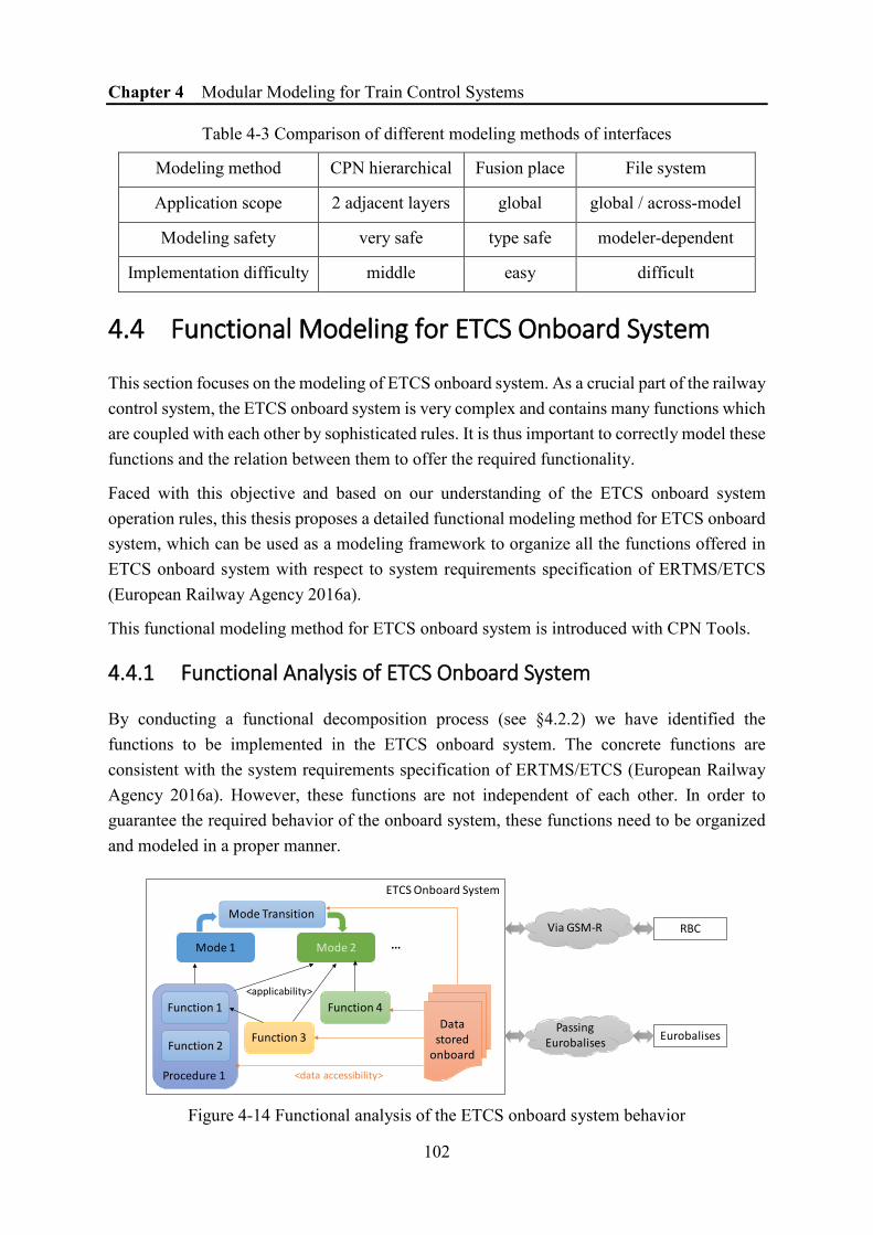
Chapter 4 Modular Modeling for Train Control Systems
102
Table 4-3 Comparison of different modeling methods of interfaces
Modeling method CPN hierarchical Fusion place File system
Application scope 2 adjacent layers global global / across-model
Modeling safety very safe type safe modeler-dependent
Implementation difficulty middle easy difficult
4.4 Functional Modeling for ETCS Onboard System
This section focuses on the modeling of ETCS onboard system. As a crucial part of the railway control system, the ETCS onboard system is very complex and contains many functions which are coupled with each other by sophisticated rules. It is thus important to correctly model these functions and the relation between them to offer the required functionality.
Faced with this objective and based on our understanding of the ETCS onboard system operation rules, this thesis proposes a detailed functional modeling method for ETCS onboard system, which can be used as a modeling framework to organize all the functions offered in ETCS onboard system with respect to system requirements specification of ERTMS/ETCS (European Railway Agency 2016a).
This functional modeling method for ETCS onboard system is introduced with CPN Tools.
4.4.1 Functional Analysis of ETCS Onboard System
By conducting a functional decomposition process (see §4.2.2) we have identified the functions to be implemented in the ETCS onboard system. The concrete functions are consistent with the system requirements specification of ERTMS/ETCS (European Railway Agency 2016a). However, these functions are not independent of each other. In order to guarantee the required behavior of the onboard system, these functions need to be organized and modeled in a proper manner.
Figure 4-14 Functional analysis of the ETCS onboard system behavior
Mode 1 Mode 2
Function 1
Function 3
Function 4
Mode Transition
ETCS Onboard System
Data stored
onboardFunction 2
Procedure 1
RBCVia GSM-R
Passing Eurobalises Eurobalises
···
<data accessibility>
<applicability>

Chapter 4 Modular Modeling for Train Control Systems
103
Figure 4-14 illustrates a functional view of the ETCS onboard system behavior. With respect to the system requirements specification of ERTMS/ETCS (European Railway Agency 2016a), the ETCS onboard system behavior can be described by three levels:
• Modes;
• Procedures;
• Functions.
It is worth noting that the term “function” in this section and in the system requirements specification (European Railway Agency 2016a) refers to the “concrete function” in the functional decomposition introduced in §4.2.2.
Modes and Mode Transitions
Modes are top-level operational states of ETCS onboard system. At any time (even if the equipment is not powered), the onboard system is considered to be in one and only one mode.
In different modes, the onboard system has different behaviors, reactions, and responsibilities. The detailed introduction to each mode can be found in §4.4.2. According to the current mode, the onboard system can execute a procedure or some functions to complete the operational tasks.
In certain specific circumstances, a mode transition is triggered by the satisfaction of one condition or a combination of several conditions. As the name implies, a mode transition will change the current mode of the onboard system.
Procedures
Procedures are mainly defined for the onboard interaction with the driver or other system components. A procedure is usually composed of a series of operations, which will lead to some major changes of the onboard system states, e.g., “start of mission” or “change of train orientation”. A procedure always has very clear entry and exit(s), it is thus described as a flowchart in the system requirements specification (European Railway Agency 2016a).
As indicated by the arrowed lines with the tag <applicability> in Figure 4-14, a procedure has its applicable mode(s), i.e., in which mode(s) the procedure can be started.
In the accomplishment of a procedure, it can execute several functions that are already defined to facilitate the operation. For example, Procedure 1 in Figure 4-14 relies on Function 1 and Function 2.
Functions
A function is defined to offer a specific operation. An example can be the “concrete functions” illustrated in Figure 4-3 in §4.2.2.

Chapter 4 Modular Modeling for Train Control Systems
104
Like the procedures, a function also has its applicable mode(s). When the onboard system is in one of its applicable modes, a function can be executed directly, it can also be used as part of a procedure, or be called by another function.
As a result of the concurrency of ETCS onboard system and the existence of lots of supervision functions, in the most modes, there are always several functions being executing in parallel.
Data stored onboard
Apart from the current mode, there are also lots of data store onboard, e.g., the speed, location. The values of these data represent the operational conditions of the whole onboard system.
The data can be accessed and modified by the three kinds of operation already introduced: mode transition, procedure, and function. The mode value can also be regarded as a special kind of data; however, the current mode can only be modified by a mode transition.
Based on the functional analysis of the ETCS onboard system behavior, we propose to functionally model the ETCS onboard system as shown in Figure 4-15. Some abbreviations are examples of names of modes or procedures, which will be introduced later.
Figure 4-15 Functional modeling for ETCS onboard system
The details of the modeling method will be proposed in §4.4.2-§4.4.5.
4.4.2 Modeling of Modes and Mode Transitions
4.4.2.1 Introduction to ETCS Modes
According to the latest version 3.6.0 of the ERTMS/ETCS system requirements specification (European Railway Agency 2016a), 17 modes are defined as follows:
• Full Supervision (FS)
• Limited Supervision (LS)
• On Sight (OS)
• Staff Responsible (SR)
• Shunting (SH)
• Unfitted (UN)
• Passive Shunting (PS)
• Sleeping (SL)
• Stand By (SB)
• Trip (TR)
Mode Transition
Procedures
Functions ···
Modes···
NP SB FSSHOS
NP
SB
SB
SH
SB
OS
OS
FS
OS
SB
OS
FS
SH
SB
SB
NP ···
···
F_023F_015 F_015 F_105 F_113 F_210
SoM EoM ShDrvData stored
onboardApplicable mode(s)
Values
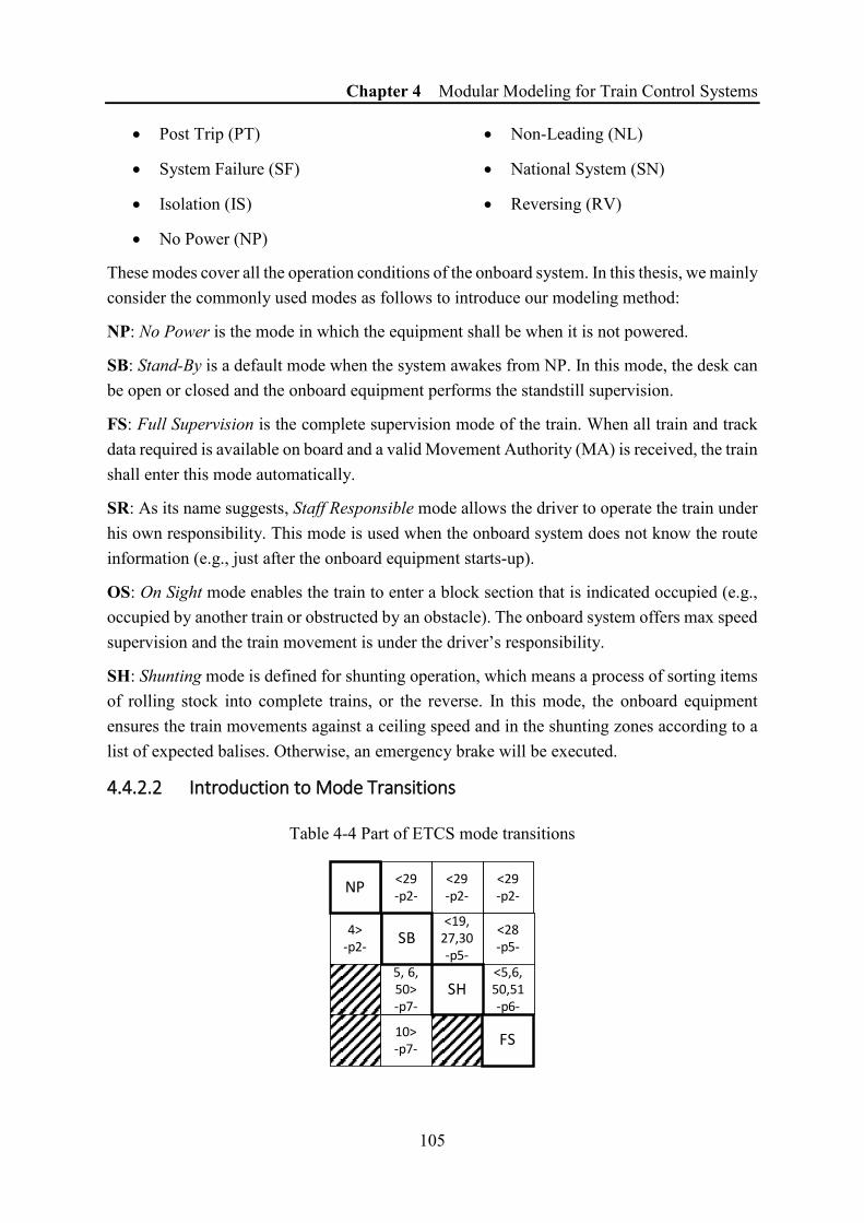
Chapter 4 Modular Modeling for Train Control Systems
105
• Post Trip (PT)
• System Failure (SF)
• Isolation (IS)
• No Power (NP)
• Non-Leading (NL)
• National System (SN)
• Reversing (RV)
These modes cover all the operation conditions of the onboard system. In this thesis, we mainly consider the commonly used modes as follows to introduce our modeling method:
NP: No Power is the mode in which the equipment shall be when it is not powered.
SB: Stand-By is a default mode when the system awakes from NP. In this mode, the desk can be open or closed and the onboard equipment performs the standstill supervision.
FS: Full Supervision is the complete supervision mode of the train. When all train and track data required is available on board and a valid Movement Authority (MA) is received, the train shall enter this mode automatically.
SR: As its name suggests, Staff Responsible mode allows the driver to operate the train under his own responsibility. This mode is used when the onboard system does not know the route information (e.g., just after the onboard equipment starts-up).
OS: On Sight mode enables the train to enter a block section that is indicated occupied (e.g., occupied by another train or obstructed by an obstacle). The onboard system offers max speed supervision and the train movement is under the driver’s responsibility.
SH: Shunting mode is defined for shunting operation, which means a process of sorting items of rolling stock into complete trains, or the reverse. In this mode, the onboard equipment ensures the train movements against a ceiling speed and in the shunting zones according to a list of expected balises. Otherwise, an emergency brake will be executed.
4.4.2.2 Introduction to Mode Transitions
Table 4-4 Part of ETCS mode transitions
<29-p2-
<29-p2-
<19,27,30-p5-
4>-p2-
5, 6, 50>-p7-
<28-p5-
<29-p2-
<5,6,50,51-p6-
10>-p7-
NP
SH
SB
FS

Chapter 4 Modular Modeling for Train Control Systems
106
Table 4-4 shows part of the ETCS mode transitions. A complete mode transitions table is defined as “Transitions Table” in (European Railway Agency 2016a), which can also be found as Table B-1 in Appendix A of this thesis.
By this example, we explicate the information implied in the mode transitions table:
- The symbol “>” or “<” indicates the transition direction;
- The numbers before the arrows “>” or “<” refer to the conditions defined in the “Transition Conditions Table” in (European Railway Agency 2016a);
- Each transition has a priority order which is indicated by “-px-”, a smaller x number has a higher priority. The use of priority is to avoid a conflict between several transitions of the same original mode when their conditions are satisfied at the same time;
- The blank cell with diagonal stripes means that there is no corresponding transition (e.g., no transitions NP→SH, NP→FS nor SH→FS in Table 4-4).
Table 4-4 can thus be translated to a more explicit form as shown in Table 4-5 with the necessary definitions of conditions.
Table 4-5 Translation to Table 4-4 (Part of ETCS mode transitions)
Origin Mode Target Mode Priority Condition(s)
NP SB p2 Cond.4
SB NP p2 Cond.2
SB SH p7 Cond.5, Cond.6 or Cond.50
SB FS p7 Cond.10
SH NP p2 Cond.29
SH SB p5 Cond.19, Cond.27 or Cond.30
FS NP p2 Cond.29
FS SB p5 Cond.28
FS SH p6 Cond.5, Cond.6 or Cond.51
Conditions:
[2] A desk is open.
[4] Onboard system is powered.
[5] “Train is at standstill” and “current level is 0 or NTC or 1” and “driver selects shunting mode”.

Chapter 4 Modular Modeling for Train Control Systems
107
[6] “Train is at standstill” and “current level is 2 or 3” and “reception of the information ‘Shunting granted by RBC’ after a shunting request initialized by the driver and”.
[10] (Valid Train Data is stored on board) and (MA + SSP + gradient parameters are on-board) AND (no specific mode is required by a Mode Profile)
[19] “Driver selects ‘exit Shunting’” and “train is at standstill”.
[27] “Desks are closed” and “function ‘Continue Shunting on desk closure’ is not active”.
[28] Desks are closed.
[29] Onboard system is NOT powered.
[30] “Desks are closed” and “no ‘passive shunting’ input signal is received”.
[50] “A request to acknowledge shunting is displayed on DMI” and “the driver acknowledges”.
[51] “A Mode Profile defining the entry of a Shunting area is used onboard” and “The max safe front end of the train is inside the Shunting area”.
We then introduce the modeling of the modes and model transitions in CPN.
4.4.2.3 Modeling of Mode and Mode Transitions in CPN Tools
Using colored Petri nets, “mode” can be declared as an enumerated colorsets 𝑀𝑀𝑀𝑀𝐷𝐷𝐸𝐸 by enumerating all its values, as shown in Code 4-3. We also declare some variable 𝑚𝑚, 𝑚𝑚𝐵𝐵𝑆𝑆𝑇𝑇1, 𝑚𝑚𝐵𝐵𝑆𝑆𝑇𝑇2 of the type 𝑀𝑀𝑀𝑀𝐷𝐷𝐸𝐸 to operate the mode value.
Code 4-3 Declarations of mode and mode transitions (part of) 1 (*Declaration of Mode and Mode Transitions*) 2 colset MODE= with
NP|SB|PS|SH|FS|LS|SR|OS|SL|NL|UN|TR|PT|SF|IS|SN|RV; 3 var m, mode1, mode2: MODE; 4 val P1=101; val P2=102; val P3=103; val P4=104; val P5=105; val
P6=106; val P7=107;
As already introduced in 4.4.2.2 there are different priorities for different mode transitions. Thanks to the support of priority inscription of transitions in CPN Tools (Westergaard and Verbeek 2011), we defined the values 𝐶𝐶1 − 𝐶𝐶7 are reserved for priority control and will be discussed later.
For the mode transitions, the basic idea to model each mode-to-mode transition by a transition in CPN. Figure 4-16 shows the modeling of the mode transition NP→SB, triggered by Condition 4 (“onboard system is powered”, “C4” for short in the model), with the priority p2. The transition is named C4_P2 to refer to condition C4 and priority P2. The input arc of transition C4_P2 is annotated with the value NP and the output arc with the value SB.
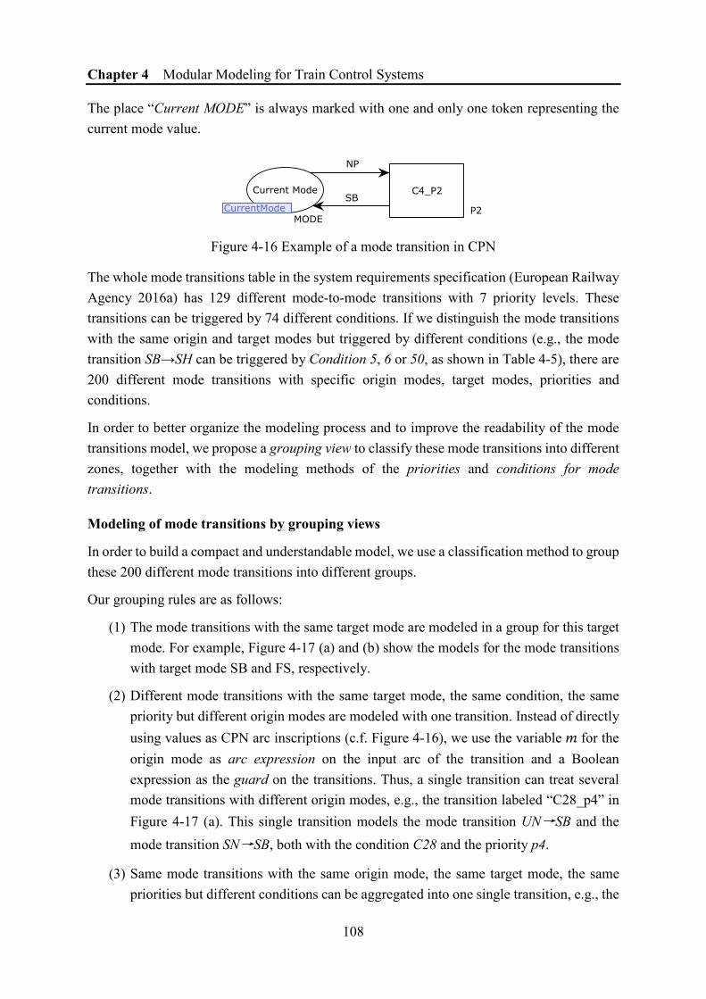
Chapter 4 Modular Modeling for Train Control Systems
108
The place “Current MODE” is always marked with one and only one token representing the current mode value.
Figure 4-16 Example of a mode transition in CPN
The whole mode transitions table in the system requirements specification (European Railway Agency 2016a) has 129 different mode-to-mode transitions with 7 priority levels. These transitions can be triggered by 74 different conditions. If we distinguish the mode transitions with the same origin and target modes but triggered by different conditions (e.g., the mode transition SB→SH can be triggered by Condition 5, 6 or 50, as shown in Table 4-5), there are 200 different mode transitions with specific origin modes, target modes, priorities and conditions.
In order to better organize the modeling process and to improve the readability of the mode transitions model, we propose a grouping view to classify these mode transitions into different zones, together with the modeling methods of the priorities and conditions for mode transitions.
Modeling of mode transitions by grouping views
In order to build a compact and understandable model, we use a classification method to group these 200 different mode transitions into different groups.
Our grouping rules are as follows:
(1) The mode transitions with the same target mode are modeled in a group for this target mode. For example, Figure 4-17 (a) and (b) show the models for the mode transitions with target mode SB and FS, respectively.
(2) Different mode transitions with the same target mode, the same condition, the same priority but different origin modes are modeled with one transition. Instead of directly using values as CPN arc inscriptions (c.f. Figure 4-16), we use the variable 𝑚𝑚 for the origin mode as arc expression on the input arc of the transition and a Boolean expression as the guard on the transitions. Thus, a single transition can treat several mode transitions with different origin modes, e.g., the transition labeled “C28_p4” in Figure 4-17 (a). This single transition models the mode transition UN→SB and the mode transition SN→SB, both with the condition C28 and the priority p4.
(3) Same mode transitions with the same origin mode, the same target mode, the same priorities but different conditions can be aggregated into one single transition, e.g., the

Chapter 4 Modular Modeling for Train Control Systems
109
transition labeled “C28_C47_p3” aggregate two mode transitions triggered by Condition 28 and Condition 47.
(4) The rules (2) and (3) above can be used together to achieve a more compact representation, e.g., the transition labeled “C31_C32_p6” in Figure 4-17 (b). It is worth noting that in this example it is necessary that each of the mode transitions LS→FS, SR→SH or OS→SH could be triggered by either Condition 31 or Condition 32.
By applying the grouping rules, we obtain a mode transition model of ETCS onboard system for 12 modes: NP, SB, PS, SH, FS, SR, OS, NL, SF, IS, RV and PT. Figure 4-17 shows part of the model of mode transitions. A complete version can be found in Figure B-1. The whole model uses 6 groups and 37 transitions to model 84 mode transitions for the 12 considered modes.
(a) Transitions with target=SB (b) Transitions with target=FS
Figure 4-17 Part of ETCS mode transitions model
It is worth noting that the places labeled “CurrentMode” use the fusion place feature in CPN Tools, details can be found in §4.3.3.3.
Modeling of conditions for mode transitions
The mode transitions need to be triggered when appropriate conditions are satisfied. This sounds like the basic enabling rules of the transitions in Petri nets, i.e., the input places are regarded as the precondition of enabling a transition.
We model the conditions for mode transitions by linking or adding some condition places as the input places of the mode transitions, as well as by using arc expressions to have more precise control on the conditions.
Figure 4-18 illustrates some mode transitions linked with their appropriate conditions modeled by some places (can be called condition places) on the right side. Each transition is connected to one or more places as a condition may be refined by several sub-conditions (e.g., Condition 46). This model can enable the corresponding mode transitions by checking the satisfaction of these (sub-)conditions.

Chapter 4 Modular Modeling for Train Control Systems
110
Figure 4-18 Conditions and priorities for mode transitions
These conditions places are always fusion places as the conditions are always some onboard data that are also used in other operations where their value shall be modified.
Colored tokens in the condition places contain values of Boolean or other types. The required values to trigger the mode transitions can be assigned on the arc expressions and thus be used to check the satisfaction of the conditions. We distinguish two kinds of values by their different treatments.
(1) The first kind of condition values belong to the general onboard data, i.e., a variable which always has a value, e.g., “train powered” (type Boolean) or “speed” (Numeric). Normally the condition place contains one and only one token which is used to specify the required value for the mode transition. The firing of the mode transition checks but does not change the value (i.e., “read-only” for the mode transition). In this case, we use a bi-directional arc to link the condition places of these “read-only” value and the mode transition.
(2) The second kind of condition values is, in fact, a semaphore to inform of an event, e.g., the onboard equipment receives a certain message, or the drive has confirmed a proposition via DMI. We also use colored tokens to represent these condition values but by a single-direction arc from the condition place to the transition if the condition is only used to trigger the mode transition and should only be used once.

Chapter 4 Modular Modeling for Train Control Systems
111
In more sophisticated cases, the guards of CPN transitions can also be used to check the satisfaction of conditions, the same way as they are used to select the origin mode in Figure 4-17 and Figure 4-18.
Modeling of Priority in Mode Transitions
The priority for different mode transitions is implemented in the CPN model by applying the priority inscription formalism offered by CPN Tools (Westergaard and Verbeek 2011). A CPN transition with higher priority is given a smaller priority value and is forced to occur before other transitions with lower priorities. The CPN transitions without an explicit priority value are assigned 𝐶𝐶_𝑁𝑁𝑀𝑀𝐸𝐸𝑀𝑀𝐴𝐴𝑁𝑁 = 1000 by default.
In Figure 4-18, all the transitions are prioritized transitions and the priority can be found at the lower left corner of each transition with the values already declared in Code 4-3. In the example model, two transitions are assigned the priority P2, one transition of P3, and the other two of P6.
In Figure 4-18 several condition places are marked and Transition “C13_p3” is the only enabled transition. According to the current marking, the condition for Transition “C13_p3” and for Transition “C46_p6” are both satisfied. However, Transition “C13_p3” has a higher priority and prevent Transition “C46_p6” from being enabled.
However, we have noticed that there exist some lots of mode transitions with the same priority. We classify the mode transitions with the same priority into two classes:
(1) Those with the contradictory conditions which can be verified by analyzing the syntax of the mode transitions model, e.g., Transition “C4_p2” and Transition “C29_p2” shown in Figure 4-18. In this example, the former is for the origin mode “NP” and the latter is for an origin mode “m≠NP”. What’s more, their Boolean conditions “powered” and “not powered” can never be satisfied at the same time.
(2) Those without syntactically contradictory conditions, e.g., Transition “C46_p6” and Transition “C59_p6” in Figure 4-18. Supposing a case that current mode is “FS”, “LS” or “OS” and the train is at standstill, it is seemingly possible that the conditions for both the two transitions might be satisfied but all depend on the constraints on these conditions.
The second class of mode transitions with the same priority interests us. As says the system requirements specification (European Railway Agency 2016a), “it is obvious that these transitions cannot occur at the same time, and so can never lead to a conflicting situation”. However, from an academic point of view, there is just a weak explanation but no explicit guarantee to ensure that the onboard system shall not simultaneously satisfy the conditions for multiples mode transitions with the same priority in the current version of the system

Chapter 4 Modular Modeling for Train Control Systems
112
requirements specification. A case study of verification to the certainty of mode transition will be introduced in §5.5.2.
4.4.3 Modeling of Procedures
4.4.3.1 Introduction to the Modeling of Procedures
A procedure defines a series of operations of ETCS onboard system, which usually contain the interactions between different subsystems and components, information exchanged, or events triggered.
In the current version 3.6.0 of ETCS system requirements specification (SRS) (European Railway Agency 2016a), 17 procedures are defined in SRS
• Start of mission
• End of Mission
• Shunting Initiated by Driver
• Override
• RBC/RBC Handover
• Level Transitions
• Train Reversing
• Change of Train Orientation
• Changing Train Data from sources different from the driver
• On-Sight
• Train Trip
• Joining / Splitting
• Indication of Track Conditions
• Limited Supervision
• Entry in Shunting with Order from Trackside
• Passing a non-protected Level Crossing
• Generation of Track Conditions related information to an ETCS external function 91
A procedure has its applicable modes and can call several functions, as already shown in Figure 4-14 and Figure 4-15. In the SRS, each procedure is illustrated by a flowchart with text annotations. It usually has one entry but may have different exits.
In this thesis study, we propose a method to build the CPN models for each procedure based on the procedure flowcharts in the SRS. The general process of this modeling method is shown as Figure 4-19.
Starting from the flowcharts in SRS, we perform the operation syntactic transformation, which syntactically transforms the flowchart into a literal PN model based on the analysis of the structure.
Then, semantic refinement and reduction can be executed several times to finally achieve a final CPN model of procedure. The semantic refinement adds or links the conditions,

Chapter 4 Modular Modeling for Train Control Systems
113
operations, etc. to the literal PN model, while the semantic reduction generates a more condensed model by conducting aggregations of states and operations.
In order to better present our modeling method of procedures, the rest of this section will be introduced based on an example of the procedure “Start of Mission” (SoM), whose flowchart is shown by Figure B-2 in Appendix A. However, we can always use some general methods to model other procedures.
Figure 4-19 General process of building CPN models for procedures
4.4.3.2 Stage 1: Syntactic Transformation
In this first stage of the modeling of procedures, we apply the following syntactic transformation rules to get a literal model based on the analysis of the structure of procedure flowchart in the requirements specification. This stage can be conducted without the railway control system domain knowledge. In this stage, the literal models may be either presented in Petri Nets (PN) or Colored Petri Nets (CPN), anyhow they will later be transformed to CPN model in the semantic refinement stage.

Chapter 4 Modular Modeling for Train Control Systems
114
We propose the syntactic transformation rules according to the different types of elements in the original flowchart. Each element in the flowchart can be transformed into a corresponding Petri net element, which is introduced as follows.
State
A state in the procedure is represented by a rectangle labeled with “S xx” in the procedure flowchart. A state can be regarded as a projection of the status of the ETCS onboard system and is composed of a specific set of onboard data.
A state often means that the onboard system is in a relatively stable state. The onboard system is considered to stay in the current state before the conditions to trigger the transition to another state are completely satisfied. A transition to a new state indicates that the system behavior in which we are interested differs from its previous state. Thus, the definition of a state is based on the modeling objective. For example, even if the train is advancing and its location is changing, it can be regarded to remain in a state as long as it does not pass a key location point, e.g., EOA (End of Authority).
The states in a procedure are transformed to places in the literal Petri net model. When the place representing a state is marked, it means the onboard system is in this particular state. Some examples can be found in Figure 4-20 (a) as shown by Places S0, S1 and S2.
Action
An Action in the procedure is represented by a rounded rectangle labeled with “A xx” in the procedure flowchart. It is transformed into a place in the literal Petri net model, as shown by some examples in Figure 4-20 (b) as A32, A33, etc. In the refinement phase, these places transformed from action may be refined in different ways according to their meaning, which will be introduced later.
Decision
A decision in the procedure is represented by a rhombus labeled with “D xx” in the procedure flowchart. It is transformed to a place in the literal Petri net model, which presents a relatively temporary state which is about to branch depending on some extra information (e.g., different choices made by the driver). Examples can be found in Figure 4-20 (a) with decision D2 and D3. These temporary states for decisions can usually be agglomerated with neighboring states in the reduction phase.
Branching arrow with decision option
A branching arrow in the flowchart just follows the decision symbol and is labeled with decision option, e.g., “yes” or “no”. It is transformed into a transition in the literal Petri net model. According to the different decision options, it will lead the system to different future states, as shown by the transitions “D2_Yes” and “D2_No” in Figure 4-20 (a). These

Chapter 4 Modular Modeling for Train Control Systems
115
transitions will be later refined by adding the conditions to model the semantics of the decision options.
Event
An event in the procedure is represented by an arrow labeled with “E xx” in the procedure flowchart. It is also transformed to a transition in the literal Petri net model, an example of the transition “E1” can be found in Figure 4-20 (a).
An event transition will lead the system to another state as the result of the occurrence of the expected event (e.g., reception of a response from other components). Similar to the branching arrows with decision option, the capturing of the event will be modeled in the refinement phase by adding appropriate conditions to the event transition.
Unlabeled arrow
There may exist some unlabeled arrows in the procedure flowchart, mainly for the reason of maintaining the structure of the procedure flowchart. These unlabeled arrows are transformed to transitions in the literal Petri net model and can be called “route transitions”. An example is the first transition in Figure 4-20 (a)These transitions might later be removed in the reduction phase due to the aggregation of its input and output places.
Figure 4-20 Literal translation rules with extract of procedure “SoM”
S0Mode is SB and desk open and no communication session is established or is being established
S1The on-board requests the driver to enter/re-validate Driver-ID, offers the driver the possibility to enter/revalidate
the Train running number and offers the driver the possibility to set/remove a Virtual Balise Cover
D2Stored position & stored level
are "valid"
E1Driver has entered/validated Driver-ID
D3Level
S2Onboard requests Driver to enter/re-validate level
No
Yes
S0
S1
S2
D2 D3
E1
D2_No
D2_Yes
A33Onboard reports "valid" position to RBC
A32Onboard informs Driver
A35RBC reports to Onboard "valid" position
A24Onboard deletes stored position data
A40Onboard informs Driver
S10Waiting for Driver selection
A32
A33
A40
A24
S10A35
Extract of Procedure “SoM” (Flowchart) Syntactic model (PN)
(a)
(b)

Chapter 4 Modular Modeling for Train Control Systems
116
Union of multiple arrows
Union of multiple arrows in the procedure flowchart are transformed into some separated transitions in the literal Petri net model which have the common output arc(s). An example can be found in Figure 4-20 (b).
After applying the above rules, all kinds of elements in the flowchart are replaced by the two basic Petri net elements – places and transitions – in the literal Petri net model.
We then use arcs to connect these places and transitions according to their connectivity in the original flowchart. We also put the text labels linked to each flowchart element on their corresponding elements in this Petri net literal model to facilitate the following refinement and reduction phases.
Figure 4-20 shows some extracted parts of the flowchart of the procedure “Start of Mission” and their corresponding Petri net literal models. A complete version of the literal model of procedure “Start of Mission” can be found in Figure B-3 in Appendix A.
This literal Petri net model is, in fact, a structural projection of the procedure flowchart in Petri Nets. It is an intermediate model because the semantics of these places and transitions in Petri net are still represented by the text labels which is not yet implemented. The implementation of the semantics will be conducted in the semantic refinement stage.
By the way, this literal Petri net model allows several kinds of the reachability verification of the procedure.
4.4.3.3 Stage 2: Semantic refinement with operations and conditions
The refinement phase is to implement the semantics of the literal Petri net model. This can be done by adding extra Petri net structures and by building the connections between the literal model of the procedure and other system models.
We distinguish structural refinement and behavioral refinement.
Structural refinement
A structural refinement is to replace some places and transitions in the literal Petri net model by refined Petri net structures according to their semantics. As shown in Figure 4-21, a place can be refined by a place-transition-place structure and a transition can be refined by a transition-place-transition structure. Thus, we refine the literal Petri net model vertically by the structural refinement.
The structural refinement is meanly to refine the elements related to the actions. We have introduced that an action in the flowchart is transformed into a place in the literal Petri net model. This place may be refined in different ways according to the semantics of the action modeled:

Chapter 4 Modular Modeling for Train Control Systems
117
- Continuous action: the system is executing a continuous action until it changes to another state (e.g., a braking until the train is standstill). The corresponding place in the literal model does not need structural refinement and remains as shown in Figure 4-21 (a). This place can be called an execution place and the condition to stop the action depends on its output transition.
- Instant action: if the place is transformed from an instant action, it can be refined by a place-transition-place structure as shown in Figure 4-21 (b). The refined structure uses two state places to model the states before and after the execution of the action, and an action transition to execute an instant action. This transition will be further refined.
- External action: the place implies an action executed by external parts of the system model, e.g., a demand to another system component or a function call. In this case, the place is first replaced by a place-transition-place structure similar to an instant action. Then the transition needs to be further refined by a transition-place-transition structure with an external parallel structure as shown in Figure 4-21 (c). Transition “Start” is an action transition to send the request or to call a function; place “wait” is a state place where the system waits the response or the result of the execution of the function called; transition “Finish” is an event transition triggered by the reception when the external action is finished. The two places “request” and “response” are all data places.
Figure 4-21 Structural refinement examples

Chapter 4 Modular Modeling for Train Control Systems
118
The objective of a structural refinement is to model all the steps in the procedure by Petri net places and transitions. The structural refinement can be done in several iterations. After finishing the structure refinement, each place or transition has one of the following semantics.
There are three categories of places after the structural refinement:
- State place, which indicates the current state in the procedure when it is marked. normally no more than one state place shall be marked in the procedure (except for a procedure with parallel flows);
- Execution place, which indicates an operation being occurred as long as the place is marked. If the concrete execution device is modeled, it may be related to this execution place in the procedure model;
- Data Place, where the onboard data are stored or exchanged. It is also used by the semaphore to synchronize the global model, e.g., a function call.
Every transition will have one of the three semantics after the refinement:
- Event transition, which represents the occurrence of an external event, e.g., the manipulation of the driver through DMI, or the reception of the balise telegrams while the train passes a Eurobalise;
- Action transition, which means that the system performs an instant action, e.g., the modification of a value of the onboard data. Compared to an execution place which models a continuous execution as long as the place is marked, an action transition implies the action is done with the firing of the transition and thus can be finished in no time.
- Route transition, which is used for the flow-control purpose in a Petri nets model for the procedure. They are used to connect different places in sequence, to represent the branching with different decision options, or to check the satisfaction of the conditions.
Behavioral refinement
After the structural refinement which vertically refines a procedure model, the number of the elements (i.e., transitions and places of Petri nets) is quasi-fixed. However, it is still necessary to implement the behavior of each element by horizontally adding some extra manipulations and establishing the relationship with other parts of the model.
The behavioral refinement is mainly conducted on the three kinds of transitions after the structural refinement. The behavioral refinement includes, but is not limited to, adding arc expressions to manipulate the appropriate colored tokens, defining transition guards to check the satisfaction of the necessary conditions, creating the connections between the refined structure and other parts within the same procedure model or in another model (e.g., via fusion place).
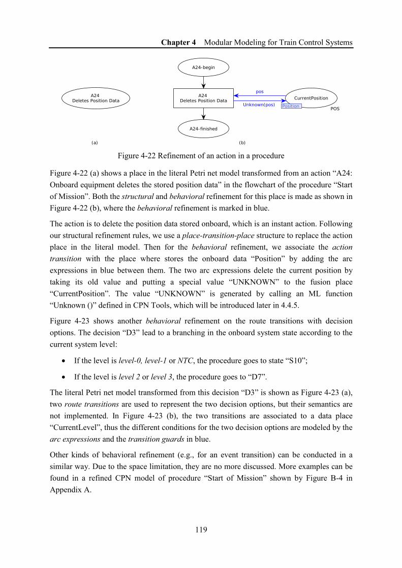
Chapter 4 Modular Modeling for Train Control Systems
119
Figure 4-22 Refinement of an action in a procedure
Figure 4-22 (a) shows a place in the literal Petri net model transformed from an action “A24: Onboard equipment deletes the stored position data” in the flowchart of the procedure “Start of Mission”. Both the structural and behavioral refinement for this place is made as shown in Figure 4-22 (b), where the behavioral refinement is marked in blue.
The action is to delete the position data stored onboard, which is an instant action. Following our structural refinement rules, we use a place-transition-place structure to replace the action place in the literal model. Then for the behavioral refinement, we associate the action transition with the place where stores the onboard data “Position” by adding the arc expressions in blue between them. The two arc expressions delete the current position by taking its old value and putting a special value “UNKNOWN” to the fusion place “CurrentPosition”. The value “UNKNOWN” is generated by calling an ML function “Unknown ()” defined in CPN Tools, which will be introduced later in 4.4.5.
Figure 4-23 shows another behavioral refinement on the route transitions with decision options. The decision “D3” lead to a branching in the onboard system state according to the current system level:
• If the level is level-0, level-1 or NTC, the procedure goes to state “S10”;
• If the level is level 2 or level 3, the procedure goes to “D7”.
The literal Petri net model transformed from this decision “D3” is shown as Figure 4-23 (a), two route transitions are used to represent the two decision options, but their semantics are not implemented. In Figure 4-23 (b), the two transitions are associated to a data place “CurrentLevel”, thus the different conditions for the two decision options are modeled by the arc expressions and the transition guards in blue.
Other kinds of behavioral refinement (e.g., for an event transition) can be conducted in a similar way. Due to the space limitation, they are no more discussed. More examples can be found in a refined CPN model of procedure “Start of Mission” shown by Figure B-4 in Appendix A.
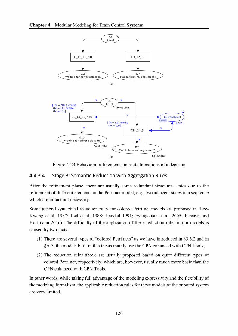
Chapter 4 Modular Modeling for Train Control Systems
120
Figure 4-23 Behavioral refinements on route transitions of a decision
4.4.3.4 Stage 3: Semantic Reduction with Aggregation Rules
After the refinement phase, there are usually some redundant structures states due to the refinement of different elements in the Petri net model, e.g., two adjacent states in a sequence which are in fact not necessary.
Some general syntactical reduction rules for colored Petri net models are proposed in (Lee-Kwang et al. 1987; Joel et al. 1988; Haddad 1991; Evangelista et al. 2005; Esparza and Hoffmann 2016). The difficulty of the application of these reduction rules in our models is caused by two facts:
(1) There are several types of “colored Petri nets” as we have introduced in §3.3.2 and in §A.5, the models built in this thesis mainly use the CPN enhanced with CPN Tools;
(2) The reduction rules above are usually proposed based on quite different types of colored Petri net, respectively, which are, however, usually much more basic than the CPN enhanced with CPN Tools.
In other words, while taking full advantage of the modeling expressivity and the flexibility of the modeling formalism, the applicable reduction rules for these models of the onboard system are very limited.

Chapter 4 Modular Modeling for Train Control Systems
121
However, some aggregation rules can still be applied to eliminate these redundant structures by analyzing their semantics. The basic idea of the reduction is based on the aggregation of a sequence of states (or operations) into an atomic state (or operation) if it is not necessary to distinguish them according to the modeling objective.
As shown in Figure 4-24, the place-transition-place structure in the zone of dotted lines is obtained by the structural refinement of two actions, and there is only a route transition without condition to connect the two sequential actions. In this case, once the system is in the state “finished” of Action 1, it will not stay there but will directly go to the place “not started” of Action 2. Thus, the place-transition-place structure in the zone of dotted line with two state places and a transition can be replaced by a single state place.
Figure 4-24 Semantic reduction with aggregation rules
Another reduction rule can be applied to an “event transition – state place – action transition” structure, where the state place does have an execution semantics. This structure can be reduced to a single transition that integrates the event and the action semantics. Due to space limitation, we do not explain this rule in detail.
It is not necessary to conduct the reduction after all the model is totally refined. In order to limit the model size, a provisional model can also be reduced before a further refinement. By this method, refinement and reduction can be conducted several times to obtain a final procedure model, as emphasized in Figure 4-19. After the semantic refinement and reduction, part of the final CPN model for the procedure “Start of Mission” is shown in Figure B-4 in Appendix A.
The semantic reduction based on aggregation rules help both to build a procedure model with improved readability and to obtain a compact model to facilitate the state-space based verification in the future phase of the system development cycle.

Chapter 4 Modular Modeling for Train Control Systems
122
4.4.4 Modeling of Onboard Functions
4.4.4.1 ETCS Onboard Function Introduction
The operation of train control systems is based on the combination of different functions. A list of onboard functions is defined in the system requirements specification (European Railway Agency 2016a), e.g., “Request MA Cyclically respect to approach of target indication point or MA timer elapsing”, “Speed restriction to ensure a given permitted braking distance” and “Override related speed restriction”.
These onboard functions, in fact, the concrete functions already introduced in §4.2.2. etc. Each function has its applicable mode(s). It can be triggered in the applicable mode(s) or be called by a procedure.
It is important to not confound an onboard function, which is a concept to describe the system behavior in our functional modeling framework, with an ML function, which is a programming technique integrated into CPN Tools to enhance the expressivity of colored Petri nets. During the modeling, we can exploit all the modeling approaches offered by CPN Tools, including the ML functions, to build the onboard system models, which surely include the models of onboard functions.
4.4.4.2 Modeling of Onboard Functions
Because of the diversity of the onboard functions and the expressive ability of modeling using CPN Tools, modelers have the flexibility to model the onboard functions according to their understandings and practice. Each function is modeled by a subpage in CPN Tools
However, we can still classify the modeling of functions under two categories which have very different modeling approaches.
• Blocking function: which is always called by a procedure or by another function. When the called function is ongoing, the execution of the caller model is blocked.
• Non-blocking function: which is activated when its conditions are satisfied. These conditions can also be set on purpose to activate the function. Anyway, the execution of the function is in parallel with any other processes.
Blocking function modeling
A blocking function can be modeled by using the hierarchical features in CPN Tools. A blocking function is modeled as a subpage with input and output ports. Then the function can be called as a substitution transition in the model of its caller, which can be a procedure or another function.
Figure 4-25 shows the subpage model of a blocking function “MA Request”. This function can form a colored token of product type “TrainxRBCxMsg” by specifying the TrainNumber,
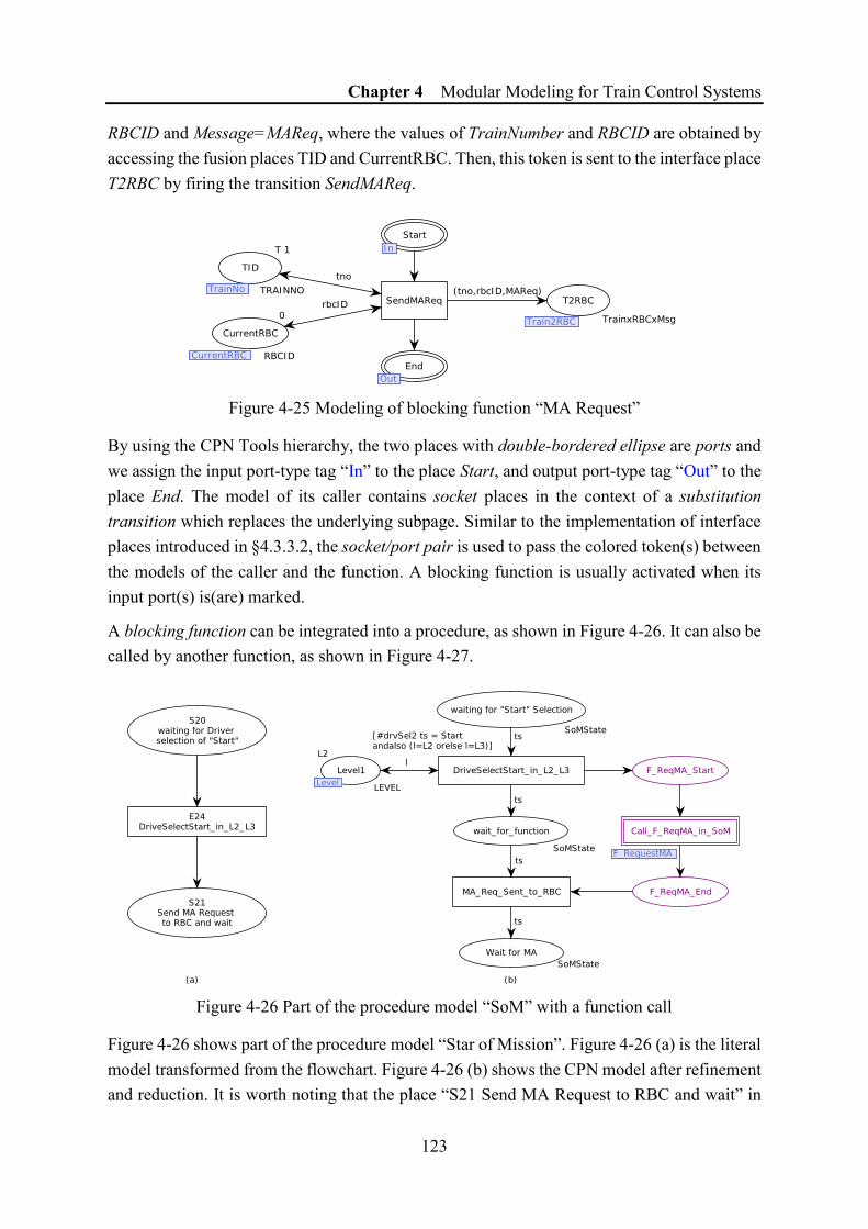
Chapter 4 Modular Modeling for Train Control Systems
123
RBCID and Message=MAReq, where the values of TrainNumber and RBCID are obtained by accessing the fusion places TID and CurrentRBC. Then, this token is sent to the interface place T2RBC by firing the transition SendMAReq.
Figure 4-25 Modeling of blocking function “MA Request”
By using the CPN Tools hierarchy, the two places with double-bordered ellipse are ports and we assign the input port-type tag “In” to the place Start, and output port-type tag “Out” to the place End. The model of its caller contains socket places in the context of a substitution transition which replaces the underlying subpage. Similar to the implementation of interface places introduced in §4.3.3.2, the socket/port pair is used to pass the colored token(s) between the models of the caller and the function. A blocking function is usually activated when its input port(s) is(are) marked.
A blocking function can be integrated into a procedure, as shown in Figure 4-26. It can also be called by another function, as shown in Figure 4-27.
Figure 4-26 Part of the procedure model “SoM” with a function call
Figure 4-26 shows part of the procedure model “Star of Mission”. Figure 4-26 (a) is the literal model transformed from the flowchart. Figure 4-26 (b) shows the CPN model after refinement and reduction. It is worth noting that the place “S21 Send MA Request to RBC and wait” in

Chapter 4 Modular Modeling for Train Control Systems
124
Figure 4-26 (a) is identified as an external action according to our structural refinement rules, regardless of its original identifier beginning with “S” which normally means a state. A reduction rule is also applied to aggregate two transitions after the refinement, before Figure 4-26 (b) is finally obtained.
The structure with pink color uses a substitution transition “Call_F_ReqMA_in_SoM”, which is in fact executed in the subpage of the function “MA Request” (Figure 4-25). The socket/port pairs are established between the function subpage and the caller model as shown in Table 4-6.
Table 4-6 Socket/port pairs in function subpage and the caller model
Direction Port places in function subpage
“MA Request” (Figure 4-25)
Socket places in the caller model
Figure 4-26 (b) Figure 4-27
Input Start F_ReqMA_Start F_ReqMA_End
Output End F_ReqMA_Start F_ReqMA_End
According to the requirement of the procedure, it is necessary to send the MA request before the procedure could be in a state “wait (for MA)”. For this reason, the “sending of MA Request” is a blocking function for the procedure. The reader may have noticed that we use a parallel structure in Figure 4-26 (b) to call the function by adding a waiting place to block the procedure. That is because in a procedure the state places usually need to be defined as an appropriate colorset (“SoMState” in the example), which cannot be processed by a general-purpose function. We will soon see that in the example of calling the same function (“MA Request”) in another function “Request MA by timer elapsing”, the called function can be directly merged into the caller’s main process without the parallel structure (Figure 4-27).
A blocking function usually models an immediate execution. A blocking function is called when the caller needs to make sure that the called function is finished before performing other operations. It can also be used to obtain an execution result which might be a data processing, in which case the ports of the function need to be defined as appropriate colorset(s) to pass the parameter and to return the result.
We benefit from the CPN Tools hierarchy to strengthen the reusability of a blocking function. Thanks to the support of the substitution transitions, CPN Tools creates an exclusive and local subpage for each substitution transition being fired. That is to say, it is possible to execute the same function in different callers at the same time, without considering the synchronization issue.
Non-blocking function modeling
Different from the blocking functions which are usually called explicitly in another operation, non-blocking functions are activated with respect to the satisfaction of the appropriate

Chapter 4 Modular Modeling for Train Control Systems
125
conditions, including mode, level, etc. and especially as a result of the occurrence of certain events, e.g., the expiration of a timer.
A non-blocking function is also modeled as a subpage, but it does not have hierarchical elements, i.e., the ports. Thus, a non-blocking function model can be executed in parallel with the all the other models (e.g., procedure models, other function models). The execution of a non-blocking completes an operation or makes some changes on the onboard data. Fusion places are frequently used in a non-blocking function model to offer the conditions or to make the changes to the onboard system.
Figure 4-27 shows the model of a non-blocking function “Request MA respect to timer elapsing of T_MAR or T_TIMEOUTRQST”. The place Start is initially marked with an uncolored token (type UNIT in CPN Tools). Two transitions T_TIMEOUTQST_Req and T_MAR_Req are associated with the corresponding places in which a Boolean token of “true” value will be generated when the timer is expired. That the calculation and management of these timers consider the approach of perturbation location or MA timer elapsing configuration, which are beyond the scope of the function in question. In Figure 4-27 we only use the Boolean value as the representation of two different events.
Figure 4-27 Modeling of the function “Request MA by timer elapsing”
The two transitions T_TIMEOUTQST_Req and T_MAR_Req can also check the satisfaction of the applicable conditions (i.e., mode and level in this example). The firing of one of the transitions is a result of both the satisfaction of the conditions and the occurrence of the specified event. Any of the two transitions can generate a token in the place F_Req_MA_Start.
The bottom part of Figure 4-27 in pink color calls the function “MA Request” that we have already introduced. It also shows that a function can be called in another function.

Chapter 4 Modular Modeling for Train Control Systems
126
After being executed once, the transition Return leads to its initial marking. So that the function can wait for a new event to be executed at another time.
From the examples, the reader can infer that the modeling method of a non-blocking function is quite different from that of a blocking function. Firstly, a non-blocking function does not have ports, it is activated as a result of the condition(s) and/or events. Secondly, a non-blocking function does not have different callers and there is only one (subpage) model for each non-blocking function in the global system. That is also the reason why a non-blocking function needs an initial marking to control the operation loop. Even if the two different events in Figure 4-27 are satisfied at the same time, the function model needs to run two times to be completed.
A large part of ETCS onboard system functionality can be modeled by non-blocking functions, especially when it is concerned to supervision purpose. Lots of non-blocking functions are ongoing in parallel and asynchronously to guarantee the good operation of the ETCS onboard system.
4.4.5 Modeling of Onboard Data
4.4.5.1 Introduction to onboard data
Similar to the modeling of most computer-based systems, we distinguish data and operations (which manipulate the data) during the modeling. This discrimination makes the modeling process clearer and the models built are easier to be implemented by programming languages in a future phase of the system development lifecycle.
We have introduced the modeling methods of three kinds of operations (i.e., mode transition, procedure and function) in §4.4.2 – §4.4.4, respectively. Along with the introduction to the modeling of these operations, we have already shown some examples of onboard data without discussing them systematically. This subsection introduces the modeling methods of onboard data.
Onboard data refer to all kinds of values stored in the onboard system such as speed, position, and even messages, etc. The values of these data may either be initially stored onboard, be obtained from the environment, or be recalculated by the onboard system during the execution. They are modeled as different data types and can be accessed and modified by appropriate operations to maintain the correct functionality of the onboard system.
4.4.5.2 Modeling method of onboard data using CPN Tools
Using CPN, a place can be used as the container of a variable of a particular type provided that the place never contains more than one token. In this case, the colorset of such a place is equal to the variable data type and the unique token in the place presents the value of the represented variable. Sometimes an empty place is also authorized, which represents an

Chapter 4 Modular Modeling for Train Control Systems
127
uninitialized variable or another particular connotation according to the modeler. Based on this idea, we introduce a more sophisticated to model the onboard data.
The principal task of modeling onboard data is to define the corresponding colorsets and to facilitate the data manipulation. CPN Tools offers abundant basic types e.g., Boolean, Integer, Real, String, Enumerated, Index, and several compound types, e.g., Product, Record, List.
According to the system requirements specification (European Railway Agency 2016a), several data have their validity besides the value.
The data validity may be in one of the three states:
• Valid: the stored value is known to be correct;
• Invalid: the stored value may be wrong;
• Unknown: no stored value available (after it is deleted etc.).
The data validity can be modified in certain special situations. For example, when the ETCS onboard system exits an old mode and enters a new mode, several data may be invalidated (thus invalid) or deleted (thus unknown).
Code 4-4 illustrates an example to model the position of a train by two colorsets “POS” and “POS_VALID”.
Code 4-4 Declaration of data with validity 1 (*Declaration of POS and its validity*) 2 colset POS=int with ~1..1000000; 3 val UNKNOWN = ~1; 4 colset POS_VALID = bool; 5 var p, q: POS; 6 var pv: POS_VALID; 7 colset POSxVALID = product POS * POS_VALID;
The colorset “POS” is defined as an integer with its boundary. The non-negative integers represent the train’s position in a coordinate system with a unit. The value “~1”(−1) is reserved to represent an “UNKNOWN” value. The product colorset “POS x VALID” is defined to have a compact representation of the two data which are always related.
Figure 4-28 Example of data manipulation in CPN models

Chapter 4 Modular Modeling for Train Control Systems
128
The onboard system model stores these data by colored tokens in some places. These data can be accessed and modified during the operation of trains, which are usually modeled by transitions. Figure 4-28 shows an example to increase and delete the train position.
It is important that a colored token of a special value is always necessary to represent the case of non-existence in the practical onboard system. The reason is that the non-existence of a special value may be a condition to operate an action. However, in Petri nets, the detection of an empty place (the non-existence of tokens) is quite difficult. Some solutions e.g., inhibitor arc, will largely increase the complexity of the modeling.
In the example of train position, we use a special value “UNKNOWN” to represent the state after the train position is deleted. Thus, the place Position is always marked with a colored token. The condition of the non-existence of the train position can be modeled by a detection of the value “UNKNOWN”.
It is also worth noting that the two colorsets POS and POS_VALID could be combined as a product colorset (which is the case in the example) or a record colorset, but should not be merged into a union colorset as shown in Code 4-5.
Code 4-5 Declaration of position by union colorset 1 (*Declaration of position by union colset*) 2 colset POS=int with ~1..1000000; 3 colset POS_Special = with InVALID | UNKNOWN;
4 colset POS_EXT = union POS + POS_Special;
The difference is that in the former case, the value POS and POS_VALID can have their values at the same time, which is useful to model a situation that a train has an invalid position value (such as the onboard system is just powered and has a stored position at the end of the last journey with a doubt that train might be moved meanwhile). However, the latter with a solution of union colorset cannot correctly model it.
Some data do not need to be modeled with validity, such as a condition, which indicates the satisfaction of an assertion (e.g., the cab is powered), or an event (e.g., timer elapsing). For the same reason of the detection of non-existence in Petri nets, a condition/event is recommended to be modeled as Boolean other than a Unit (neutral) type, as shown in Table 4-7.
Table 4-7 Modeling of conditions and events
Modeling method Condition Event
Satisfaction Non-satisfaction Happened Not happened
Recommended true: bool False: bool true: bool False: bool
Not recommended

Chapter 4 Modular Modeling for Train Control Systems
129
4.5 Modeling of Railway Node with Automated Routing Function
4.5.1 Routing Function in a Railway Node
The automatization of a train control depends on the interaction and cooperation of both the onboard system and the trackside system. As an important part of the trackside system, a railway node (see §2.2.1.2) allows the passthrough of trains according to their itineraries, which is implemented by the train routing function.
In reality, train routing is still a manual function in rail systems even with the use of ERTMS/ETCS. We propose here a model allowing to consider the automatic assignment of an appropriate route to each train arriving at the entrance of a node.
To better illustrate our proposition, let us consider a railway node example in the global abstracted system model previously introduced in Figure 4-6 which has a concrete structure as shown in Figure 2-1. The railway node is supposed to have a unique operation direction. It has two entrances (A and B) and two exits (C and D).
We have introduced the concept route, which is an itinerary from an entry to an exit in a railway node. From the point of view of train control, a route can be characterized by the resources that the train must use during its itinerary, e.g., tracks, signals and points (c.f., §2.2.2). By defining an interlocking table in the form of Table 4-8, the necessary resources can be reserved for a particular train to pass the node.
Table 4-8 Example of an interlocking table
No. In Out Signal Tracks* Points**
1 A C s1 tc01, tc03, tc05, tc07, tc09, (tc11) pt1, pt2
2 B D s2 tc02, tc04, tc06, tc08, tc10, (tc12) pt3, pt4
3 A D s1 tc01, tc06, tc08, tc10, (tc12) pt4, pt1(r), pt3(r)
4 B C s2 tc02, tc04, tc06, tc09, (tc11) pt3, pt2(r), pt4(r)
5 A C s1 tc01, tc06, tc09, (tc11) pt1(r), pt2(r), pt3(r), pt4(r)
In the interlocking table, each route is assigned a route number, together with its resources, i.e., the signal protecting the route, the tracks composing the route and the points in the route. The points with “(r)” after their identifiers need to be locked in the reverse position while the others in normal position. The tracks in brackets show the first track after the route, which is usually necessary to be reserved together with the other resources in the same route.

Chapter 4 Modular Modeling for Train Control Systems
130
Figure 4-29 CPN model for railway node module

Chapter 4 Modular Modeling for Train Control Systems
131
Each railway node has its own structure different from another and has thus a particular interlocking table. The information listed in the interlocking table needs to be integrated into the railway node model, which makes it possible to automatically select an appropriate route for the trains passing the node.
However, as our modeling objective is to offer a reusable module, the railway node structure and the corresponding interlocking table information should not affect the modeling of the component model. In other words, the structure of the railway node module should be independent of the interlocking table logic. By following the component modeling method of the parametric module, we present a modeling method to express the interlocking table information by compound colored tokens in one of its parameter places.
4.5.2 Modeling of railway node component using CPN Tools
The railway node model is shown in Figure 4-29. Some related declarations are defined in Code 4-6.
Code 4-6 Declarations for a railway node module 1 colset TrainID = index T with 1..10; 2 colset Station = with StationA | StationB | Station C | Station
D | NodeN; 3 colset TRAIN = product TrainID * Station * Station ; 4 colset Connect = with A | B | C | D | unknown; 5 colset RBC2Node= product MsgType * Station * Connect * TRAIN ; 6 colset NodeTRAIN = product TRAIN * Connect * Connect; 7 colset TCID = index TC with 1..12; 8 colset PID = index PT with 1..4; 9 colset NR = with Nm | Rv; 10 colset Point = product PID * NR; 11 colset SID = index Signal with 1..4; 12 colset RouteDetail = product RouteID * Connect * Connect * SID
* PTList * TCList; 13 colset TRAINxRouteID = product TRAIN * RouteID; 14 colset RouteIDxBOOL = product RouteID * bool;
The principal function of this railway node model is to set a route which allows the passage of the train automatically.
We suppose that when a train is approaching the railway node, the RBC that manages the train issues a route request by generating a token of TypeRouteReq into the place RBC2Node. This route request contains the train’s information and the entrance it is approaching.
The first task for the railway node model is to determine an exit from which the train is supposed to leave the node. The decision of this exit depends on the train’s destination station.

Chapter 4 Modular Modeling for Train Control Systems
132
An ML function NodeSchedule() on the output arc inscription of transition ReceiveRouteReq implements this task. Then a token of type NodeTRAIN is put in place ScheduledTrain.
In order to better explain the functions of the railway node model, we consider an example of colored token of type NodeTRAIN ((Train(1), StationA, StationC), (A,C)) in place ScheduledTrain. The implied information is shown as Table 4-9. This example will also be used to explain the following process of the railway node model.
Table 4-9 Example of a Token of Type NodeTRAIN
TrainID Origin Destination Node entrance Node exit
Train (1) Station A Station C A C
As shown in the left part of Figure 4-29, Transition CheckResources checks the possibility of setting a route from entrance A to exit C. The corresponding resources are indicated by the tokens in places Idle Routes, Available Tracks and Available Points, which represent respectively the routes that have not been set, the tracks and the points that have not been taken by another route.
Place Routelib also plays a vital role as it contains the tokens of type RouteDetail that store the information describing how each route is composed, according to the interlocking table as shown in Table 4-8. Since the arcs connected to place Routelib are all bi-directional arcs, the tokens will never be really removed. However, they are used to create the correct binding elements for transition CheckResources. An example of two tokens representing Route(1) and Route(5) are shown in Table 4-10 in the form of a multiset.
Table 4-10 Example of tokens of type RouteDetail
1`(Route(1), A, C, Signal(1), [(PT(1), Nm), (PT(2), Nm)], [TC(1), TC(2), TC(3), TC(4), TC(5), TC(11)]) ++ 1`(Route(5), A, C, Signal(1), [(PT(1), Rv), (PT(3), Rv), (PT(4), Rv), (PT(2), Rv)], [TC(1), TC(8), TC(5), TC(11)])
We suppose that all the resources in Node N are available when the route request of Train(1) is received. In this case, for transition CheckResources, two binding elements are possible: the binding element of Route(1) and another of Route(5).
Assume that the binding element of Route(5) is chosen and transition CheckResources is fired, the relevant resources will be taken and a token of type TRAINxRouteID will be put into place WaitforPoints. Transition CheckResources also sends a command to the part of point switch (place PointOrder) in order to change the corresponding points into desired positions and then lock them.

Chapter 4 Modular Modeling for Train Control Systems
133
Our model does not contain functions of the infrastructure like switch machines, so we just use a simple transition LockPts to simulate this process and give the result of this operation. If for any reasons the necessary points are not correctly positioned and locked, transition CheckPoints receives a token with a bool variable false. Then the route request will be canceled, and all the resources already taken will be released and the token representing the route request will be put again in place ScheduledTrain.
If the points are positioned and locked as desired, a token of type TRAINxRouteID is put into place ReadyToSet then transition SetRoute is fired. After that, the token is transferred into place ReadyRoute, the protective signal of this route is then set to be green (a token indicating the route is put into Place Route2Signal). The node sends the route information to the train, and it informs the train’s next RBC (the one managing the block sections that the train will enter after passing through the node). So far, the route is finally set, and the train is expected to go through it.
After the train has successfully passed the route and arrived in the first block of the line managed by a new RBC, the new RBC sends a message of TypeRegAck to inform the node. Transition TrainPassed is then fired to unlock the route and release the resources.
We point out that the functions of some infrastructure equipment (e.g. point machines, signals) are not included in our model. These devices are actually the concrete actuators of the railway systems. Consequently, this study only considers the control of these devices rather than model their concrete behavior.
4.5.3 Perspectives of modeling a railway node
The railway node model realized the “automated routing” function of a railway node, based on a fixed interlocking table. However, there are also studies for a dynamic routing strategy in a railway node, which allocates (locks) and retrieves (releases) the necessary resources in a dynamic and more efficient way. A dynamic routing could mean:
- The fixed interlocking table is replaced by an algorithm that can calculate a route when the train is approaching;
- The occupied resources in a route could be released gradually (e.g., track by track) along with the train’s passage to improve the resources utilization;
- An assigned and even occupied route might be altered again according to the real-time change of the resources, with respect to safety rules.
The use of such a dynamic routing will certainly improve the passthrough capacity of a railway node. However, as a safety-critical system, the railway operators need a safety guarantee before a new strategy could be implemented. Thus, a perspective of an improved railway node model could be to implement the dynamic routing in Petri nets which can be formally verified.

Chapter 4 Modular Modeling for Train Control Systems
134
4.6 General WFN Modeling Patterns: Application for RBC Modeling
4.6.1 Modeling of RBC Component using WFN
In this section, we pose several problems in terms of modeling and then propose solutions.
The first problem we want to illustrate here is how to model the behavior of a train system component from a functional point of view. We are interested here in the modeling of some functions related to the movement authority (MA) management, no longer in the ETCS onboard component as introduced in §4.4, but this time on the trackside, implemented by the RBC component.
The second problem that we want to address in this section is the necessary compromise for a designer between the modeling expressivity and the analysis facility. Generally speaking, the stronger expressiveness a modeling formalism has, the more difficulty one meets when it comes to the analysis. For example, we use CPN Tools to model the complex system behaviors of the onboard system (§4.4) and railway node (§4.5) taking advantage of its expressivity and flexibility. However, the use of some extensions of CPN Tools, e.g., the list structure, could bring a difficulty to make the formal verification on models built with these extensions (Xie et al. 2017a; Xie et al. 2017b).
In order to facilitate a posteriori stage of verification, we were thus interested in formalisms with better analyzability. Based on the discussion of different Petri net classes in §3.3.1, well-formed Petri nets (WFN) (Chiola et al. 1991a) is a variant of colored Petri nets created for the aim of “ease of analysis” and with some constraints of modeling. This study makes an attempt to model the complex DES using WFN, by taking the movement authority function in the RBC component as an example.
As a trade-off choice between the expressivity and analyzability of colored Petri net variants, WFN also brings some inconvenience to the modeling phase of a complex train control system, compared to the general colored Petri nets or some enhanced variants as that used in CPN Tools. These constraints and inconvenience could be a challenge to build complex DES models using WFN with its syntactical constraints.
In the modeling practice, one could be faced with some system structure or behavior that is difficult to be modeled using WFN, especially when it comes to asymmetry behavior or data manipulation. We identify three useful kinds of modeling formalism which are supported by CPN Tools and some other colored Petri net variants but are not supported in WFN. These formalisms are necessary to model the RBC component with respect to our modeling objective.

Chapter 4 Modular Modeling for Train Control Systems
135
In the first part of this section (§4.6.2), we propose three general modeling patterns in WFN, which allows the implementation of the same formalisms while respecting the WFN constraints. In the second part (§4.6.3), these WFN modeling patterns are applied in the modeling of the desired functions of the RBC component. However, the application of these general modeling patterns could be much larger and extended to any other similar complex DES modeled with WFN.
4.6.2 General WFN Modeling Patterns for Complex DES
In this section, we propose three practical modeling patterns to increase the WFN’s usability and thus the productivity without sacrificing its theoretical foundation.
These modeling patterns are:
• An equivalent alternative structure in WFN to the “if-then-else” expression available in CPN Tools;
• The definition and implementation of a “predecessor function” in WFN based on the existing successor function;
• A “list structure” in WFN with the corresponding operations on it, i.e., inserting an item, removing an item, modifying a value, querying a value.
A case study that uses all these modeling patterns is the modeling of the RBC component of a railway control system. This RBC model in WFN is introduced in §4.6.3.2.
4.6.2.1 Conditional arc modeling in WFN
The conditional arc with “if-then-else” expression is a powerful structure facilitating the modeling of diverse behaviors caused by different conditions, which is commonly used by almost all the structured programming languages. In several colored Petri net variants or tools such as CPN Tools, such a conditional arc is supported, which is, unfortunately, not the case in WFN.
This thesis study proposes two WFN equivalent structures which have the same semantics of the conditional arc. One solution is based on guarded functions, the other is based on transitions with the guard.
Notation
Consider a transition 𝑡𝑡 and a place 𝑇𝑇. Let ∁(t) = 𝐶𝐶1 × 𝐶𝐶2 × ⋯ × 𝐶𝐶�.
Considering a post-incidence function Wpost(𝑇𝑇, 𝑡𝑡) on the arc connecting the transition t and one of its output places 𝑇𝑇 ∈ 𝑡𝑡• (or respectively, a pre-incidence function Wpre(𝑇𝑇, 𝑡𝑡) on the arc connecting the transition t and one of its input places 𝑇𝑇 ∈ 𝑡𝑡 • ), which is a conditional arc with a general “if-then-else” expression:

Chapter 4 Modular Modeling for Train Control Systems
136
Wpost (pre)(𝑇𝑇, 𝑡𝑡) = 𝑇𝑇𝐼𝐼 𝑀𝑀 𝑡𝑡ℎ𝑇𝑇𝑇𝑇 𝐹𝐹� 𝑇𝑇𝐵𝐵𝑠𝑠𝑇𝑇 𝐹𝐹� (4-4)
Where 𝑀𝑀 is a condition defined on ∁(t). 𝐹𝐹� and 𝐹𝐹� are two unguarded colored functions from
∁(t) to the multiset of ∁(p), which can also be expressed by sums of a tuple of basic functions in WFN.
𝐹𝐹� = � �𝐼𝐼1
�, 𝐼𝐼2�, … , 𝐼𝐼�
���
𝐹𝐹� = � �𝐼𝐼1�, 𝐼𝐼2
�, … , 𝐼𝐼���
�
(4-5)
The “if-then-else” expression 𝑊𝑊 ����(���)(𝑇𝑇, 𝑡𝑡) is not supported by WFN syntax, we propose two equivalent approaches to represent the same semantics.
Conditional arc modeling based on guarded functions
We define the equivalent function 𝑊𝑊����� (���)(𝑇𝑇, 𝑡𝑡) to replace Equation (4-4).
WEpost (pre)(p, t) = [g] 𝐹𝐹� + [¬g] 𝐹𝐹� (4-6)
Equation (4-6) has the same semantics of Equation (4-4) and it can be transformed to a form
that respects the definition of WFN standard functions, as shown in Equation (4-7).
WEpost (pre)(p, t) = [g] 𝐹𝐹� + [¬g] 𝐹𝐹�
= [g] � ⟨f1t , f2
t ,…, fkt ⟩
m+[¬g] � �f1
f , f2f ,…, fk
f �n
= � [g]⟨f1t , f2
t ,…, fkt ⟩
m+ � [¬g]�f1
f , f2f ,…, fk
f �n
(4-7)
Conditional arc modeling based on transitions with guard
An alternative solution to model the conditional arc in WFN is to use two transitions with their guards to model the "then" clause and "else" clause respectively. This solution is pretty useful for some software that does not support the concept of guarded function.
Figure 4-30 Modeling of conditional arc based on transitions with guard
𝑊𝑝𝑜𝑠𝑡 𝑝 𝑡 =

Chapter 4 Modular Modeling for Train Control Systems
137
Figure 4-30 (a) shows an example of a conditional arc as an output arc of transition 𝑡𝑡 with the
“if-then-else” expression 𝑊𝑊�����(𝑇𝑇, 𝑡𝑡). 𝐺𝐺 is the guard of transition 𝑡𝑡 (it is possible that 𝐺𝐺 =
𝑇𝑇𝐸𝐸𝑇𝑇𝐸𝐸, i.e., transition t does not have a guard) while g is the condition in the “if-then-else” expression.
We propose an equivalent structure to replace transition t by two transitions 𝑡𝑡� et 𝑡𝑡� . The model with a conditional arc in Figure 4-30 (a) is replaced by a structure shown as Figure 4-30 (b) by defining an equivalent WFN model
𝑊𝑊𝐹𝐹𝑁𝑁′ = (𝐶𝐶′, 𝑇𝑇′, ∁′, 𝑊𝑊 post, 𝑊𝑊 pré, Φ′) (4-8)
where:
- 𝐶𝐶′ = 𝐶𝐶 ; 𝑇𝑇′ = 𝑇𝑇 \ {𝑡𝑡} ∪ �𝑡𝑡�, 𝑡𝑡�� ;
- ∁′�𝑡𝑡�� = ∁′�𝑡𝑡�� = ∁(t) ; ∀𝑠𝑠 ∈ 𝐶𝐶′ ∪ 𝑇𝑇′ \ �𝑡𝑡�, 𝑡𝑡��, ∁′(𝑠𝑠) = ∁(𝑠𝑠) ;
- 𝑊𝑊 ����′�𝑇𝑇, 𝑡𝑡�� = 𝐹𝐹�,𝑊𝑊 ����′�𝑇𝑇, 𝑡𝑡�� = 𝐹𝐹�,𝑊𝑊 ��e′�𝑇𝑇, 𝑡𝑡�� = 𝑊𝑊 ��e′�𝑇𝑇, 𝑡𝑡�� = 𝑊𝑊 pre(𝑇𝑇, 𝑡𝑡) ;
- ∀𝑇𝑇′ ≠ p ∈ 𝐶𝐶′, 𝑊𝑊 ∗′� 𝑇𝑇′, 𝑡𝑡�� = 𝑊𝑊 ∗′� 𝑇𝑇′, 𝑡𝑡�� = 𝑊𝑊 ∗( 𝑇𝑇′, 𝑡𝑡), where ∗ ∈ {𝑇𝑇𝐵𝐵𝑠𝑠𝑡𝑡, 𝑇𝑇𝑉𝑉é} ;
- ∀𝑡𝑡′ ∈ 𝑇𝑇′ \ �𝑡𝑡�, 𝑡𝑡��, ∀𝑇𝑇′ ∈ 𝐶𝐶′, 𝑊𝑊 ∗′( 𝑇𝑇′, 𝑡𝑡′) = 𝑊𝑊 ∗( 𝑇𝑇′, 𝑡𝑡′), where ∗ ∈ {𝑇𝑇𝐵𝐵𝑠𝑠𝑡𝑡, 𝑇𝑇𝑉𝑉é} ;
- Φ′�𝑡𝑡�� = G⋀g, Φ′�𝑡𝑡�� = G⋀¬g ; ∀𝑡𝑡′ ∈ 𝑇𝑇′ \ �𝑡𝑡�, 𝑡𝑡��, Φ′(𝑡𝑡′) = Φ(𝑡𝑡′) ;
The proposition has been illustrated with an output arc of transition 𝑡𝑡. If the conditional arc is
one of the input arcs of transition 𝑡𝑡 , the analogue solution is to replace 𝑊𝑊�����(𝑇𝑇, 𝑡𝑡) by
𝑊𝑊����(𝑇𝑇, 𝑡𝑡).
4.6.2.2 Predecessor function and its WFN implementation
In WFNs the successor function ⊕ 𝐸𝐸�� (also denoted as 𝐸𝐸 + 1 by using the variable X to
replace the identity function 𝐸𝐸��) is defined as an elementary function. While in some modeling
practice, it is also necessary to use a predecessor function, which is not defined in WFNs.
We propose to define a predecessor function that can be denoted as ⊝ 𝐸𝐸��.With respect to
some application constraints, a model using predecessor functions can be represented by an equivalent WFN model using only successor functions with the same behavior.
Let ⊝ 𝐸𝐸��(𝑐𝑐) be an application from 𝑐𝑐 ∈ 𝐶𝐶 = 𝐶𝐶1
�1 × ⋯ × 𝐶𝐶��� to the predecessor element of 𝑐𝑐�
� in an ordered class 𝐶𝐶�. Similar to the successor function, it will also be denoted as 𝐸𝐸 − 1 after
replacing the identity function 𝐸𝐸�� by a variable X. It is worth noting that in an ordered class,
the predecessor of the first element in 𝐶𝐶� is the last element.

Chapter 4 Modular Modeling for Train Control Systems
138
To benefit from the features of WFN, we propose to transform a colored net using predecessor functions defined above to an equivalent WFN.
Figure 4-31 (a) shows an example of a colored net using predecessor defined above, it could be transformed to an equivalent WFN model as shown in Figure 4-31 (b).
Figure 4-31 WFN realization of a predecessor function
In Figure 4-31, ∁(𝑡𝑡) = 𝐶𝐶1 × 𝐶𝐶1; X, 𝑌𝑌 are two variables representing two identity functions 𝐸𝐸 = 𝐸𝐸1
1, 𝑌𝑌 = 𝐸𝐸12; (𝐸𝐸 − 1) and (𝐸𝐸 + 1) are notations of predecessor and successor functions
that (𝐸𝐸 − 1) = ⊝ 𝐸𝐸11, (𝐸𝐸 + 1) = ⊕ 𝐸𝐸1
1. For variable Y there are similar notations.
Figure 4-31 (a) uses the predecessor function (𝐸𝐸 − 1) in the output arc of transition t. In order to replace this structure by an equivalent WFN, we follow the two steps:
Step 1:
Search for all the instances of the variable X in the “context of transition 𝑡𝑡”, which includes the arcs connected with transition t and the guard of transition t. Then replace them with the corresponding successor function (𝐸𝐸 + 1).
It is worth noting that the three atomic predicates defined in WFN are replaced by the following rules, respectively:
- [𝐸𝐸 = 𝑌𝑌] is replaced by (𝐸𝐸 + 1);
- [𝐸𝐸 = (𝑌𝑌 + 1)] is replaced by [(𝐸𝐸 + 1) = (𝑌𝑌 + 1)], and finally [𝐸𝐸 = 𝑌𝑌];
- [X ∈ D] is replaced by [(𝐸𝐸 + 1) ∈ D], which is not in the valid form for a WFN guard. In this case, let 𝐷𝐷 = {𝑥𝑥� ⋯ 𝑥𝑥�} be a subclass, we define a new subclass 𝐷𝐷′ ={𝑥𝑥�−1 ⋯ 𝑥𝑥�−1} where 𝑥𝑥�−1and𝑥𝑥�−1 are the predecessors of 𝑥𝑥� and 𝑥𝑥�, respectively. Then [(𝐸𝐸 + 1) ∈ D] is transformed to [𝐸𝐸 ∈ 𝐷𝐷′].
In the example, the two instances are found in the guard of transition t and on the output arc from the transition t respectively in Figure 4-31 (a), which are then replaced by (X+1) in Figure 4-31 (b).
Step 2:
Replace the predecessor function (𝐸𝐸 − 1) in the “context of transition 𝑡𝑡” by the variable 𝐸𝐸.
Cl = {1. . 5}
(a) (b)
p1
C1
p2
C1
p3
C1xC1
t
[ X=Y]X
Y
( (X-1) , Y )p1
C1
p2
C1
p3
C1xC1
t
[ (X+1) = Y]X+1
Y
(X, Y)

Chapter 4 Modular Modeling for Train Control Systems
139
In the example, the predecessor function (𝐸𝐸 − 1) found in the output arc of transition t in the model of Figure 4-31 (a), is replaced by the variable 𝐸𝐸 in Figure 4-31 (b).
Application constraints:
In order that the replacement above can be performed, for a color instance 𝐸𝐸�� , if the
predecessor function ⊝ 𝐸𝐸�� is used, the corresponding successor function ⊕ 𝐸𝐸�
� cannot appear in the context of the same transition t. In other words, we cannot use the predecessor and the
successor function of a same color instance 𝐸𝐸�� simultaneously and in the “context of a
transition”.
4.6.2.3 Modeling of the list structure in high-level Petri nets
In high-level Petri nets (e.g., WFN, Colored Petri nets), the set of colored tokens in a particular place are called a multiset. The colored tokens in such a multiset may differ from each other and do not have priority. In a Petri net example shown in Figure 4-32, there are five colored tokens in place p1 (or, in the multiset of place p1) which may be different from each other. Among these five colored tokens, transition t1 is fired by choosing one token randomly.
Figure 4-32 Multiset in Petri nets
While modeling practical systems, one is often confronted with the need to model a structure of multiple elements of the same type but with an order or a priority. Lots of examples can be found as a communication protocol with a FIFO (First-In First-Out) buffer, or a queue of trains in a railway line in the railway control system in which the first train needs to be first served.
In colored Petri nets, when a transition is enabled by different binding elements, the choice from these binding elements is, in fact, to assign the token priority to different tokens in a multiset. Some solutions are proposed by using different Petri nets extensions. For example, FIFO nets (Memmi and Finkel 1985) proposed to use places with FIFO property; while in CPN Tools, the advanced data type “list” and ML code segment can also be used to change the random selection behavior, in a manner like a programming language (WANG et al. 2008). However, the Petri nets models using these new features and extensions are usually only analyzable within the tools that support these extensions. One is always confronted with some difficulties when it comes to the analysis and verification methods proposed on some general colored Petri nets variants, including the analysis convenience proposed by WFN.
This study proposes a technique to model a “list” structure, which attaches an order to the different colored tokens in a multiset without creating a new type. We use the basic structures

Chapter 4 Modular Modeling for Train Control Systems
140
supported by general high-level Petri nets to implement this list structure and propose necessary operations such as item insert, item removal, value modification, value query.
To help the reader better understand the proposition, it is illustrated in this thesis by a practical modeling pattern of a list of multiple trains in the RBC component model in WFN. It is worth noting that this technique can also be applied to other variants of high-level Petri nets other than WFN, and to any other similar list structure in any other domains.
The RBC manages multiple trains in an area of a railway line. It regards these trains under management as a list. In the RBC model in WFN, it is also necessary to have a centralized place to store this list of trains. Based on the necessity to implement the offer the basic movement authority (MA) function, the stored information should include at least the identifier and the position of each train, as well as the order of the sequence of the trains.
Using WFN, we define color class and color domain to illustrate the train identifier, position, and other necessary information.
Declarations
CLASS POS = < 0 >∪< 1, 2, … , N >∪< END >; CLASS TID = < T(0), T(1), T(2), … , T(M) >;
DOMAIN TRAINITEM = < POS, TID, POS >.
(4-9)
The color class TID enumerates the different identifiers of trains, where does not represent a real train. The value T(0) is reserved as a special value and its usage will be explained later.
The color class POS is defined as an ordered and is divided into three static subclasses. Each position in <1, 2, …, N> represents a particular block in the railway line (which has N blocks; where N is consequently a parameter that is bound to a specific value for each real line). The other two subclasses <0> and <END> are for special purposes and will be explained in the following paragraphs, where END is a constant defined by END = N + 1 for the convenience of the illustration.
The color domain TRAINITEM is a 3-tuples Cartesian product color domain. We illustrate how to establish an ordered relation among the different tokens of color domain TRAINITEM by firstly introducing the connotation it implies.
The connotation of a token of color domain TrainItem
The color domain TRAINITEM has 3 fields with their connotations shown in Figure 4-33. For each token of color domain TRAINITEM, the value of the first filed (type: POS) is the train’s current position, the value of the second filed (type: TID) is the identifier of the train. The third field of each token stores a position value (type: POS), which is the position of its preceding train. Thus, all the tokens of TRAINITEM are linked together to form a “list” structure.

Chapter 4 Modular Modeling for Train Control Systems
141
Figure 4-33 Structure and connotation of TRAINITEM tokens
We need (m + 1) tokens of color domain TRAINITEM to model a list of m trains. Figure 4-34 shows an example of a 3-trains list presented by 4 tokens of color domain TRAINITEM. We first introduce some special tokens to help the reader understand this proposition.
TrainQueueRear: the token “TrainQueueRear” in Figure 4-34 doesn’t represent a real train and should be regarded as a pointer to the position of the last train (i.e., the train in the rear position of the queue). The first and second fields of a “TrainQueueRear” token are always “0: POS” and “T0: TID”. Its third field indicates the position of the last train. We have introduced that the value “0: POS” and “T(0): TID” are reserved values and do not represent a physical position nor a train. This token always exists in the multiset to model the trains’ list even if the real trains’ list is empty.
First Train: The first train in the queue refers to the one that does not have a preceding train in the railway line area managed by this RBC. Thus, we give a special value “END: POS” to its third field where END is defined as a constant outside the valid range of the physical position value (e.g., END = N + 1). Thus, the value END is used to indicate the end of the list.
Figure 4-34 Example of a train list of three trains
More generally, in each token of type TRAINITEM, an extra field is added, and it has the same type as another value filed (can be called “linking filed”). This extra field is assigned the same value of the linking filed of its neighbor element. By this method, we form a chain through the tokens to form the list. The linking direction is alternative according to the modeling objective.
It is worth noting that our illustrative example is a little special as the position value of a token can, in fact, imply its order in the list by being compared with all the others. However, in a more general case, the values of the linking filed do not need to indicate the list order, a token for an item in the list is modeled as:
(𝐵𝐵𝑇𝑇𝑇𝑇𝑙𝑙𝑇𝑇𝑇𝑇𝑀𝑀 𝐼𝐼𝑇𝑇𝐵𝐵𝑇𝑇𝑆𝑆, 𝑎𝑎𝑡𝑡𝑡𝑡𝑉𝑉𝑇𝑇𝑏𝑏𝑡𝑡𝑡𝑡𝑇𝑇 1, 𝑎𝑎𝑡𝑡𝑡𝑡𝑉𝑉𝑇𝑇𝑏𝑏𝑡𝑡𝑡𝑡𝑇𝑇 2, … , 𝑎𝑎𝑡𝑡𝑡𝑡𝑉𝑉𝑇𝑇𝑏𝑏𝑡𝑡𝑡𝑡𝑇𝑇 𝑇𝑇, 𝑇𝑇𝑥𝑥𝑡𝑡𝑉𝑉𝑎𝑎 𝐼𝐼𝑇𝑇𝐵𝐵𝑇𝑇𝑆𝑆) (4-10)
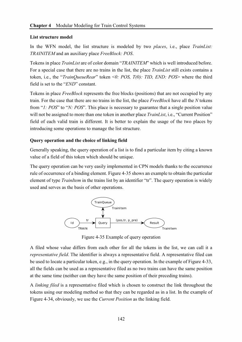
Chapter 4 Modular Modeling for Train Control Systems
142
List structure model
In the WFN model, the list structure is modeled by two places, i.e., place TrainList: TRAINITEM and an auxiliary place FreeBlock: POS.
Tokens in place TrainList are of color domain “TRAINITEM” which is well introduced before. For a special case that there are no trains in the list, the place TrainList still exists contains a token, i.e., the “TrainQueueRear” token <0: POS, T(0): TID, END: POS> where the third field is set to the “END” constant.
Tokens in place FreeBlock represents the free blocks (positions) that are not occupied by any train. For the case that there are no trains in the list, the place FreeBlock have all the N tokens from “1: POS” to “N: POS”. This place is necessary to guarantee that a single position value will not be assigned to more than one token in another place TrainList, i.e., “Current Position” field of each valid train is different. It is better to explain the usage of the two places by introducing some operations to manage the list structure.
Query operation and the choice of linking field
Generally speaking, the query operation of a list is to find a particular item by citing a known value of a field of this token which should be unique.
The query operation can be very easily implemented in CPN models thanks to the occurrence rule of occurrence of a binding element. Figure 4-35 shows an example to obtain the particular element of type TrainItem in the trains list by an identifier “tr”. The query operation is widely used and serves as the basis of other operations.
Figure 4-35 Example of query operation
A filed whose value differs from each other for all the tokens in the list, we can call it a representative field. The identifier is always a representative field. A representative filed can be used to locate a particular token, e.g., in the query operation. In the example of Figure 4-33, all the fields can be used as a representative filed as no two trains can have the same position at the same time (neither can they have the same position of their preceding trains).
A linking filed is a representative filed which is chosen to construct the link throughout the tokens using our modeling method so that they can be regarded as in a list. In the example of Figure 4-34, obviously, we use the Current Position as the linking field.

Chapter 4 Modular Modeling for Train Control Systems
143
Generally speaking, the most intuitive choice is to use an identifier filed as the linking filed, i.e., to use Train ID other than Train Position in the example. Thus, our choice of the linking filed rewards a little discussion.
Considering our practical modeling objective, the list of trains is used in the RBC component, whose major functions include the generation of MA. The calculation of EOA position in an MA for a particular train needs the querying of the position of its preceding train (a train can advance until the position of its preceding train c.f. §4.6.3.2).
Thus, it is very convenient to use the Train Position (other than the Train ID) as the linking field and to use the linking direction from the train in question to the one that precedes it. With this configuration, the extra field in each token represents the position of its preceding train. This extra field not only helps to form the the list of trains, but also facilitates query operation, which contributes to a more compact model.
In the example, we use the position as the representative field, and the linking direction is considered to facilitate the gain of the position of the preceding train, as this information is useful to generate an MA (see §4.6.3.2 for MA generation algorithm).
Operation: item insert
The insert operation adds a new train to the rear position of the list (i.e., the new train will be the last train in the queue) to model that a train just enters the area managed by this RBC. In this example, a new train will always have the position value “1: POD”.
Besides the adding of a new token that represents the new train, the insert operation needs to modify two concerned tokens already existing in the place TrainList to maintain the linking chain, i.e., the “TrainQueueRear” token, and the “LastTrain” token before the insert operation.
This operation is shown in Figure 4-36. where tr is the identifier of the train to insert, and p_last is the position of the last train before executing this inserting operation.
Figure 4-36 Example of the insert operation in a list
Two special cases need some more discussion:
- If there is already a train in block 1 (the first block in the area) before the insert operation, the token <1: POS> should not be found in place FreeBlock, the new train to be inserted needs to wait until this block 1 is set free again;

Chapter 4 Modular Modeling for Train Control Systems
144
- If the list is previously empty, the insert operation can correctly insert the train by setting its third field to the value p_last = END: POS.
Operation: item removal
The removal operation removes the first train who is leaving the area managed by RBC. This train to be removed is always found on the last block (Position N). Its token in the place TrainList to be removed has the value <N: POS, tr: TID, END: POS> where tr is the identifier of the train to be removed.
The removal operation is modeled in Figure 4-37. For the place TrainList, the removal operation removes the token <N: POS, tr: TID, END: POS>, and updates the token of its successor train <p1: POS, t1: TID, N: POS> to <p1: POS, t1: TID, END: POS> as the later has become the first train. For the place FreeBlock, the token of the block <N: POS> is released and thus be put to place FreeBlock.
Figure 4-37 Example of removal operation in a list
It is worth noting that:
- When the train to be removed is the only train in the list, it does not have a successor train. In this case, the “TrainQueueRear” token is updated and then becomes the only token in the place TrainList with its value <0: POS, T(0): TID, END: POS>, which means the list is empty;
- The variable “tr: TID” is in fact not necessary to identify the token to be removed, as we know that it must be found in the position “N”. However, in the example, we still use the train identifier “tr” to guarantee that the right train is removed.
Operation: value modification
Generally speaking, the value modification can update some information of a particular item in the list structure without altering its order. In the example of the list of trains, the only value to update is the position of a train when it advances to another block. We do not consider the overtaking on the railway line so the update to the train position does not affect the trains’ order of in the queue.
Figure 4-38 illustrates the WFN implementation of this operation. Two tokens in the place TrainList need to be updated. The update operation is done by executing two transitions.
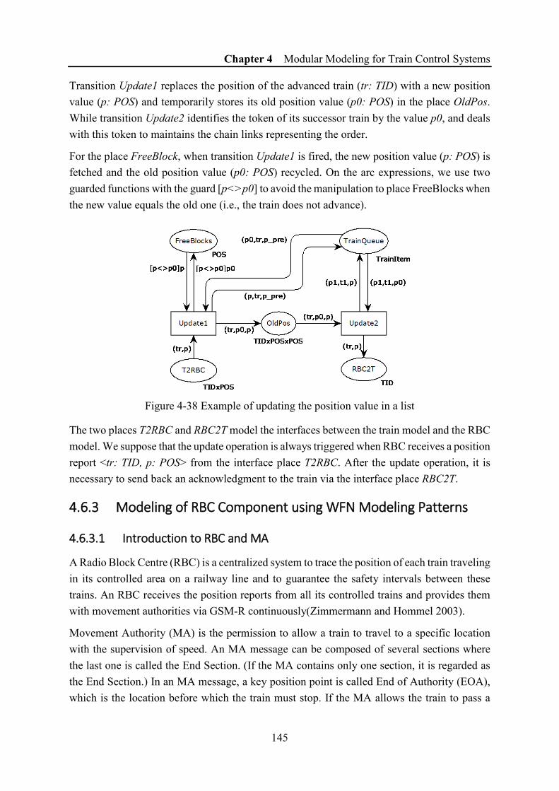
Chapter 4 Modular Modeling for Train Control Systems
145
Transition Update1 replaces the position of the advanced train (tr: TID) with a new position value (p: POS) and temporarily stores its old position value (p0: POS) in the place OldPos. While transition Update2 identifies the token of its successor train by the value p0, and deals with this token to maintains the chain links representing the order.
For the place FreeBlock, when transition Update1 is fired, the new position value (p: POS) is fetched and the old position value (p0: POS) recycled. On the arc expressions, we use two guarded functions with the guard [p<>p0] to avoid the manipulation to place FreeBlocks when the new value equals the old one (i.e., the train does not advance).
Figure 4-38 Example of updating the position value in a list
The two places T2RBC and RBC2T model the interfaces between the train model and the RBC model. We suppose that the update operation is always triggered when RBC receives a position report <tr: TID, p: POS> from the interface place T2RBC. After the update operation, it is necessary to send back an acknowledgment to the train via the interface place RBC2T.
4.6.3 Modeling of RBC Component using WFN Modeling Patterns
4.6.3.1 Introduction to RBC and MA
A Radio Block Centre (RBC) is a centralized system to trace the position of each train traveling in its controlled area on a railway line and to guarantee the safety intervals between these trains. An RBC receives the position reports from all its controlled trains and provides them with movement authorities via GSM-R continuously(Zimmermann and Hommel 2003).
Movement Authority (MA) is the permission to allow a train to travel to a specific location with the supervision of speed. An MA message can be composed of several sections where the last one is called the End Section. (If the MA contains only one section, it is regarded as the End Section.) In an MA message, a key position point is called End of Authority (EOA), which is the location before which the train must stop. If the MA allows the train to pass a

Chapter 4 Modular Modeling for Train Control Systems
146
target position with a speed not higher than an authorized speed other than to stop, this target position point is then called a Limit of Authority (LOA).
MA is used to avoid the collision of trains. With respect to its MA, the train can advance safely without collision risk to the EOA (or to the LOA at authorized speed). In order to not stop and restart (or frequently decelerate and accelerate), the MA stored in the train needs to be updated before the train approaches its EOA (or LOA).
During the travel, the train will regularly send MA requests to RBC when the onboard system is in certain modes with supervision (e.g., FS). RBC generates a new MA according to the location of the train who requires MA, the position of other concerning trains traveling in the same area, the railway line condition, and the railway signaling regulations.
In this thesis study, we simplify the generation algorithm and the update mechanism of MA for the modeling practice. In terms of MA generation, we suppose that the RBC allows a train to advance as far as the anterior block to the current position of its predecessor train recorded in the RBC. And the update of MA is always supposed to be initiated by the onboard system by sending MA request.
Apart from the generation of MA, an RBC has other functions, for examples:
• the registration and disconnection of trains;
• the acceptance of the position report from a train and the update of its position
• RBC handover, which allows the train to pass the boundary of two RBCs without stopping or even slowing down;
• the communication with other trackside systems, e.g., the interlocking system in a railway node, Traffic Control Center (TCC);
• the transmit of Temporary Speed Restriction (TSR) messages and emergency messages to the trains it managed.
Based on our modeling objectives, we only consider the simplified versions of train registration, train cancellation, train position update and communication with railway node to offer the basic RBC functions.
4.6.3.2 Modeling of RBC model in WFN
By using the abstracted system structure shown in Figure 4-6, we suppose that an RBC control all the railway line area between two stations (or nodes). In the RBC controlled area, all the trains travel in a unique direction. Figure 4-39 models such an RBC in WFN. An RBC model to control a railway line area of double tracks (each for a travel direction) can be easily obtained by duplicate the model.
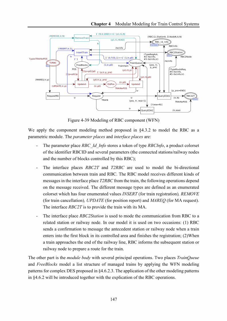
Chapter 4 Modular Modeling for Train Control Systems
147
Figure 4-39 Modeling of RBC component (WFN)
We apply the component modeling method proposed in §4.3.2 to model the RBC as a parametric module. The parameter places and interface places are:
- The parameter place RBC_Id_Info stores a token of type RBCInfo, a product colorset of the identifier RBCID and several parameters (the connected stations/railway nodes and the number of blocks controlled by this RBC);
- The interface places RBC2T and T2RBC are used to model the bi-directional communication between train and RBC. The RBC model receives different kinds of messages in the interface place T2RBC from the train, the following operations depend on the message received. The different message types are defined as an enumerated colorset which has four enumerated values INSERT (for train registration), REMOVE (for train cancellation), UPDATE (for position report) and MAREQ (for MA request). The interface RBC2T is to provide the train with its MA.
- The interface place RBC2Station is used to mode the communication from RBC to a related station or railway node. In our model it is used on two occasions: (1) RBC sends a confirmation to message the antecedent station or railway node when a train enters into the first block in its controlled area and finishes the registration; (2)When a train approaches the end of the railway line, RBC informs the subsequent station or railway node to prepare a route for the train.
The other part is the module body with several principal operations. Two places TrainQueue and FreeBlocks model a list structure of managed trains by applying the WFN modeling patterns for complex DES proposed in §4.6.2.3. The application of the other modeling patterns in §4.6.2 will be introduced together with the explication of the RBC operations.

Chapter 4 Modular Modeling for Train Control Systems
148
Train Registration (Transition InsertTrain)
We consider that a train with its identifier tr initializes a registration process by sending to RBC a message of type INSERT when it is in the first block of the RBC controlled area (i.e., Block 1). Thus, a token (INSERT, tr, 1) is received in the interface place T2RBC and transition InsertTrain can be fired. This transition applies the “item insert” operation of the WFN list structure to add a new train to the list of trains. It also sends a message of TypeRegAck to the place RBC2Station to inform the connected station or railway node, from which the train comes from, that the train has successfully passed the station or railway node.
In the model shown in Figure 4-39, the RBC considers sending an MA message to each train who just finishes the registration. Thus, the transition InsertTrain also generates a token of the train identifier to the place Request to activate the MA request operation, which will be introduced later.
Train Disconnection (Transition RemoveTrain)
We suppose that when a train is about to pass the last block (Block N) in the RBC controlled area and to enter in a station or a railway node, it sends a message of type REMOVE to the RBC, which allows removing this train from the list of trains by firing the transition RemoveTrain. This transition applies the “item removal” operation of the WFN list structure to remove the first train that is leaving the RBC controlled area.
Position Update (Transitions Update1 and Update2)
After receiving a position report message of type UPDATE, the two transition Update1 and Update2 implement the “value modification” operation of the WFN list structure to update the train’s position. In the model shown in Figure 4-39, for simplicity purposes, we regard the position report as an MA request (i.e., the train requests a new MA each time it sends a position report to RBC). That is why a token of the train identifier is also put in the place Request to activate the MA request operation.
MA Generation (Transitions QueryEOA1 and QueryEOA2)
We consider several situations in which an MA should be generated: (1) just after the train registration ( the firing of the transition InsertTrain); (2) the reception of a position report which is also regarded as MA request for convenience (after firing the transition Update2); (3) the reception of an explicit MA request message of type MAREQ. In all these three cases, a token of the train identifier “tr” is put into the place Request in the RBC model to activate the MA generation.
By applying our modeling assumptions in §4.2.4.2, a complete MA message is simplified to the EOA position. We consider the generation of an MA with the maximum possible length for each train to obtain the traveling efficiency.

Chapter 4 Modular Modeling for Train Control Systems
149
Figure 4-40 shows the algorithm to calculate the EOA position of the train who requests its MA.
Figure 4-40 Algorithm of the EOA calculation in the RBC model
If the considered train is the first train in the railway line (i.e., no trains are in front of it), it can advance until the last block of this railway line, so its EOA will be the block N. Otherwise, the EOA is related to the position of its predecessor train. Suppose that the predecessor train is in the block “𝑇𝑇_𝑇𝑇𝑉𝑉𝑇𝑇” according to the list of trains stored in the RBC model, its EOA should be the block “𝑇𝑇_𝑇𝑇𝑉𝑉𝑇𝑇 − 1”.
Figure 4-41 EOA algorithm implementation in WFN
This selective structure is usually expressed by a conditional arc with the “if-then-else” expression “ EOA = if (p_pre = END) then 𝑁𝑁 else (𝑇𝑇_𝑇𝑇𝑉𝑉𝑇𝑇 − 1) ”, which is not directly supported by WFN. We apply the WFN modeling pattern of the conditional arc (by guarded transitions) proposed in §4.6.2.1 and implement it with two transitions QueryEOA1 and QueryEOA2 as shown in Figure 4-41.
Chapter 4 Modular Modeling for Train Control Systems
150
However, the expression in the else clause (𝑇𝑇_𝑇𝑇𝑉𝑉𝑇𝑇 − 1) also contains a predecessor function, which is not originally supported in WFN, either. We apply the solution introduced in §4.6.2.2 to replace it with an equivalent structure. The two transitions QueryEOA1 and QueryEOA2 in Figure 4-39 show the final model compatible with WFN by applying a substitution 𝑇𝑇𝐵𝐵𝑎𝑎 =𝑇𝑇_𝑇𝑇𝑉𝑉𝑇𝑇 − 1, we also remind the readers that 𝐸𝐸𝑁𝑁𝐷𝐷 = 𝑁𝑁 + 1.
The firing the transition QueryEOA1 implies that it is the first train approaching the subsequent station or a railway node. Thus, this transition also generates a route request in the place RBC2Station to inform the station or railway node forward.
4.7 Conclusion of Chapter 4
The chapter focuses on the modeling methods of colored Petri nets for the train control system, which is regarded as an example of complex, large-scale, concurrency and communication-based discrete event system.
The contribution of this chapter can be classified into three categories:
• A systematical modeling methodology for a whole railway control system;
• Petri net modeling techniques for complex discrete systems,
• Practical models with respect to the European standard of train control systems
We propose a modeling methodology by considering two degrees of modularity to reduce the complexity of the train control system, i.e., the structural decomposition and the functional decomposition. Faced with a certain modeling objective, the two kinds of decomposition are mapped together in order to create an abstracted system for the ease of modeling. Some structural modeling methods are demonstrated to allows the modeling of a global railway system by components and interfaces. Focused on the onboard system, we illustrate the functional modeling methods to systematically implement the behavior by different abstract levels, i.e., modes, procedures, functions, and data. It is worth noting that these methods may be further improved and applied to similar complex DES in various domains other than train control systems.
In terms of modeling techniques, we illustrate the necessary compromise between the expressivity and the analyzability of a formalism. The well-formed nets (WFN) appear to be a better formalism than the CPNs (with CPN Tools’ extensions) from the point of view of the formal verification, despite its less powerful modeling expressivity. We propose some modeling patterns in WFN to enhance it expressivity while maintaining all its advantages for the future analysis. These patterns are proposed faced with the obstacles while modeling the RBC in a railway control system, but they are in fact general techniques to facilitate the modeling of a complex system including data manipulation. Thus, the techniques widen the

Chapter 4 Modular Modeling for Train Control Systems
151
applications of WFN of modeling, some of them can even be used for reference in the modeling practice with other kinds of colored Petri nets.
Finally, the thesis study demonstrates the possibility of modeling a whole railway control system using colored Petri nets. The study offers several practical component models which can be used as modeling bricks in further research. The ETCS onboard system component and the railway node component in CPN Tools, while the RBC component is modeled in WFN. This choice also shows that by using our modeling methodology, the encapsulation of the internal behavior of a component masks the details of its implementation and thus allows the use of complementary formalisms to implement each component.
The modeling of the onboard system is consistent with the latest standard of ERTMS/ETCS system requirements specification (UNISIG 2008); the RBC model implements the principal movement authority management functions in the scope of ERTMS/ETCS level 2; the railway node models consider the automated routing operation and we also give our perspectives of it.
In order that these components could be integrated into a systematic development approach, it is necessary to ensure that they have good properties to be implemented in a safety-critical system. This is finally the subject of a next chapter which deals with the formal verification of the models proposed in this chapter.

153
Chapter 5 VERIFICATION METHODS OF TRAIN CONTROL SYSTEM
5.1 Introduction to Chapter 5
The combinatorial explosion is the major difficulty for all the system design phases. In the modeling phase, the use of high-level Petri nets and the Petri net extensions offers compact representations of data and action, making it possible to create Petri net models for large-scale and complex systems. However, these modeling formalisms cannot avoid the huge size of models, which leads to the difficulty of the analysis of the total model.
Formal methods are highly recommended to be used with safety-critical systems development. However, for large-scale and complex DES, the combinatorial explosion problem in the formal verification is inevitable. As a result, the industrial application still prefers to use informal verification methods.
In this chapter, we propose to use formal methods for a complex train control system based on high-level Petri net models.
§5.2 introduces the verification and analysis techniques of Petri nets, especially for CPN models built in CPN Tools. We are most interested in the state space method because it can be automated, and it allows the verification of user-specified properties. Several reduction techniques can also be used to alleviate the famous state space explosion problem.
However, these state space verification techniques are still critical to be applied to the CPN models of the whole train control system that we have proposed in Chapter 4. The large system scale, the ubiquitous concurrency and the synchronism between different components make the verification stage especially problematic.
Faced with the verification on such a global system, §5.3 introduce several modular verification methods which are useful for verifying large-scale and complex system modeled by Petri nets. These modular methods share a common ground that the verification for the global system can be achieved by conducting several verifications in relatively smaller scopes. The modular methods reduce the verification’s complexity in a higher-level and can be used together with the traditional state space techniques introduced in §5.2.
In §5.4 we propose a state reduction method applicable to generate a global but reduced state space for a system composed of reactive components. We identify the execution semantics and configure the transition priority to avoid the generation of unnecessary states caused by

Chapter 5 Verification Methods of Train Control System
154
the concurrence of different components which are not useful for the verification. This technique can be applied to Petri net models of complex DES with similar configuration.
In the following sections of Chapter 5, we introduce some case studies of different kinds of verification.
§5.5 shows the verification related to mode transitions of ETCS onboard system, where §5.5.1 emphasizes the model checking of standard Petri nets properties using ASK-CTL, §5.5.2 shows the verification of a user-specified property and the possibility to use compositional verification and on-the-fly technique.
§5.6 presents the verification of the Movement Authority (MA) function via a case that a train advances by following another. This case study is complex due to both the complexity of MA generation and the heterogeneity of modeling formalism (module Train is modeled using CPN while module RBC is modeled using WFN). We use assume-guarantee method to deal with this case and the result shows that the safety property is verified but the follower train cannot extend its MA once it is stopped due to a design defect. We discuss the cause and give the solution.
5.2 Formal Verification and Analysis Techniques of Petri Nets Models
In §3.2.5, we have briefly introduced several formal verification approaches of complex DES. Since we have chosen colored Petri nets as modeling formalism, this section concentrates on the formal verification and analysis methods of Petri net models.
Petri nets models can be formally analyzed either by using a state-space exploration method, or by directly analyzing the structure of the model without an execution, e.g., the invariants computation (Murata 1989).
The state space exploration method is one of the most important approaches to computer-aided validation and verification (Bérard et al. 2001). The basic idea is to construct a directed graph representing all reachable states and state changes of the system. The main advantages of state space exploration include their high-level automation in industrial application and the possibility of investigating the user-specified properties of the underlying system.
The invariants computation method can give some general information about the Petri nets by calculating the places invariants and/or transitions invariants (Narahari and Viswanadham 1986), which allows the verification of certain properties such as boundedness or liveness.
For a complex system, the desired properties are usually not easy to write as a result of both the complexity of the system model and the use of formal languages for the property description. Details of property description are discussed in §5.2.3.

Chapter 5 Verification Methods of Train Control System
155
Since we have chosen CPN Tools as a major modeling tool, we discuss the compatible verification and analysis techniques for models built in CPN Tools in §5.2.4.
5.2.1 Formal Verification Based on State Space Methods
5.2.1.1 Model Checking
Model checking (Bérard et al. 2001) is a technique to verify the correctness of finite-state systems which is widely applied in software and industrial fields.
The key idea behind the model checking approach is shown in Figure 5-1.
Figure 5-1 Process of model checking
In order to validate that a system satisfies certain properties, the following three elements are necessary:
• The system modeled in (or transformed to) a form supported by the model checker, e.g., state space;
• The desired properties represented by a certain specification language, e.g., by temporal logic;
• The verifier technique that checks the satisfaction of the properties on the system model(s). If a property is not valid, one (or some) counterexample(s) will be returned, based on which the users can identify the errors in the model and correct them. The inner mechanism of a model checker is not necessary to be understood by its final users.
The systems to be model checked are often modeled using Transition System (Kripke structure), Petri nets, etc. Petri nets offer a compact and expressive approach for modeling complex DES. However, for the verification purpose, Petri net models need to be transformed to state space for verification purpose.
State space (also called occurrence graph, reachability graph or reachability tree) is a set of all the states with the transition rules of a system model. Most of the developed model-checking techniques are based on state space. The transformation from a Petri net model to its state space is called state space construction or generation. When a state space is obtained
System models
Abstracted properties
Model checker
System properties validated
System properties not satisfied
System to verify
Propertiesto verify
System modeling
Properties modeling
Counterexample(s)
State Space
Transform

Chapter 5 Verification Methods of Train Control System
156
from a CPN model, each node in the state space represents a reachable marking, while each arc represents the occurrence of a single binding element, leading from the marking of the source node to the marking of the destination node.
The basic idea of the state space methods is thus to present all the reachable states as well as the state changes of the Petri net model as a directed graph where the nodes represent states and arcs represent occurrences of events. State space can be constructed fully automatically and can be used to verify a large set of behavior properties using model checking techniques.
A major obstacle of the state space method is the famous state explosion problem (Valmari 1998), which means that the state space becomes exponentially larger due to the size and the complexity of the highly concurrent industrial systems. The combinatorial explosion often results in the impracticability of the exploration of the whole state space.
Another difficulty to analyze a complex system model using model checking method is the expression of the properties, i.e., the modeling of properties.
The following part of §5.2.1 will be focused on these two aspects.
5.2.1.2 State space construction and exploration
By mapping each marking in the Petri net model onto a node and each transition (with a particular firing mode for colored Petri nets) onto a directed edge, the state space can be obtained as a transition system reachable from the initial marking. An exhaustive algorithm of state space construction for ordinary Petri nets is shown as Algorithm 1.
Algorithm 1 State space construction
Step 1: Add the initial marking 𝑚𝑚0 in the GRAPH as the ROOT and mark it NEW.
Step 2: While a marking marked NEW exists, do:
a) Select a marking 𝑚𝑚 marked NEW;
b) If no transitions are enabled at 𝑚𝑚, then mark 𝑚𝑚 DEAD-END;
c) for all enabled transition 𝑡𝑡 at 𝑚𝑚 such that 𝑚𝑚�
→ 𝑚𝑚′ do:
i. Obtain the marking 𝑚𝑚′ that results from firing 𝑡𝑡 at 𝑚𝑚;
ii. If 𝑚𝑚′ does not appear in the GRAPH then add 𝑚𝑚′ and mark it NEW;
iii. Draw an arc with label 𝑡𝑡 from 𝑚𝑚 to 𝑚𝑚′ (if not already present).
Step 3: Output the GRAPH.
For a Petri net model, the state space construction is usually automated. For hierarchical Petri nets, the state space is computed from the flattened model. The use of time and data extensions often yields an infinite reachability graph, which makes its analysis intractable in the general case. Techniques such as state class graphs have been defined in the case of T-Time Petri nets
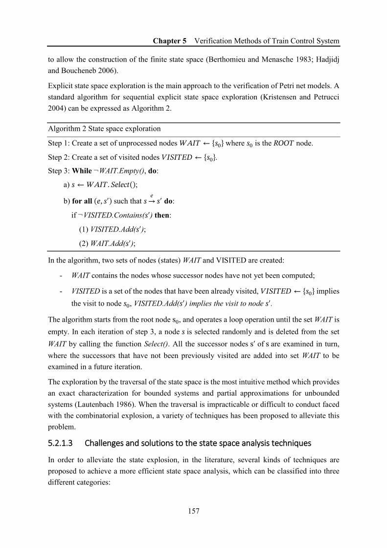
Chapter 5 Verification Methods of Train Control System
157
to allow the construction of the finite state space (Berthomieu and Menasche 1983; Hadjidj and Boucheneb 2006).
Explicit state space exploration is the main approach to the verification of Petri net models. A standard algorithm for sequential explicit state space exploration (Kristensen and Petrucci 2004) can be expressed as Algorithm 2.
Algorithm 2 State space exploration
Step 1: Create a set of unprocessed nodes 𝑊𝑊𝐴𝐴𝐼𝐼𝑇𝑇 ← {𝑠𝑠0} where 𝑠𝑠0 is the 𝐸𝐸𝑀𝑀𝑀𝑀𝑇𝑇 node.
Step 2: Create a set of visited nodes 𝑉𝑉𝐼𝐼𝑆𝑆𝐼𝐼𝑇𝑇𝐸𝐸𝐷𝐷 ← {𝑠𝑠0}.
Step 3: While ¬WAIT.Empty(), do:
a) 𝑠𝑠 ← 𝑊𝑊𝐴𝐴𝐼𝐼𝑇𝑇. 𝑆𝑆𝑇𝑇𝐵𝐵𝑇𝑇𝑐𝑐𝑡𝑡();
b) for all (𝑇𝑇, 𝑠𝑠′) such that 𝑠𝑠�
→ 𝑠𝑠′ do:
if ¬VISITED.Contains(𝑠𝑠′) then:
(1) VISITED.Add(𝑠𝑠′);
(2) WAIT.Add(𝑠𝑠′);
In the algorithm, two sets of nodes (states) WAIT and VISITED are created:
- WAIT contains the nodes whose successor nodes have not yet been computed;
- VISITED is a set of the nodes that have been already visited, 𝑉𝑉𝐼𝐼𝑆𝑆𝐼𝐼𝑇𝑇𝐸𝐸𝐷𝐷 ← {𝑠𝑠0} implies the visit to node 𝑠𝑠0, VISITED.Add(𝑠𝑠′) implies the visit to node 𝑠𝑠′.
The algorithm starts from the root node s0, and operates a loop operation until the set WAIT is empty. In each iteration of step 3, a node 𝑠𝑠 is selected randomly and is deleted from the set WAIT by calling the function Select(). All the successor nodes s′ of s are examined in turn, where the successors that have not been previously visited are added into set WAIT to be examined in a future iteration.
The exploration by the traversal of the state space is the most intuitive method which provides an exact characterization for bounded systems and partial approximations for unbounded systems (Lautenbach 1986). When the traversal is impracticable or difficult to conduct faced with the combinatorial explosion, a variety of techniques has been proposed to alleviate this problem.
5.2.1.3 Challenges and solutions to the state space analysis techniques
In order to alleviate the state explosion, in the literature, several kinds of techniques are proposed to achieve a more efficient state space analysis, which can be classified into three different categories:

Chapter 5 Verification Methods of Train Control System
158
(a) Generation of condensed state space, which allows merging some “similar” states into an abstract state during the state space generation process;
(b) Reduction of state space, which uses transformation techniques to reduce the full state space to a smaller one by preserving the properties under analysis;
(c) On-the-fly method, which conducts the construction and the exploration of state space at the same time and can stop the construction under a certain condition;
(d) More efficient exploration and storage optimization of state space;
(e) The combination of multiple state space analysis techniques.
(a) Condensed state space techniques
An example of condensed state space generation for colored Petri nets is Symbolic Reachability Graph (SRG) (Chiola et al. 1991a; Chiola et al. 1992; Chiola et al. 1997). Symmetries can often be found in the CPN models of large DES systems, which may lead to lots of repetitions or similar compositions in their reachability graphs. Symbolic Reachability Graph is proposed for the sake of analysis efficiency, which groups the symmetrical states into equivalence classes. Instead of representing all the states, only the representative marking of each class is included in the graph. As the states in the same class share similar behaviors, most of the properties are preserved and can be analyzed in a condensed form. In order to allow a fully automated construction procedure for the Symbolic Reachability Graph, the system should be modeled with Well-Formed nets (WFN), a syntactically restricted class of Colored Petri nets.
(Haddad et al. 1995) extends the original SRG method to support “partially symmetrical” systems by proposing an “Extended Symbolic Reachability Graphs”. (Ilié and Ajami 1997) shows how to conduct CTL* model checking on SRG.
(b) Reduced state space techniques
It is possible to generate a reduced state space by maintaining some properties of Petri net models that are useful for the verification. Reduction of state space can be applied in different ways according to the properties under analysis. We introduce the Strongly Connected Components (SCC) method and the partial-order reduction techniques as two examples.
For some properties based on reachability and connectivity, the SCC method can be used. The reduction idea is to use an abstract SCC to represent several states that are strongly connected (Cheng et al. 1996) and thus obtain a corresponding SCC graph which has a smaller size than the ordinary reachability graph. The model checking on SCC mainly maintains reachability properties (liveness, home marking, etc.). The SCC graph transformation tool is integrated into the software CPN Tools. An efficient CTL-like model checking method ASK-CTL (Christensen and Mortensen 1996) can be executed on an SCC graph.

Chapter 5 Verification Methods of Train Control System
159
Another approach to obtaining a reduced state space can be based on partial-order reduction as shown in Figure 5-2. In asynchronous systems, different independent concurrent processes are interleaved, the order of their executions may not have an effect on the system but will generate many redundancy states. Partial-order reduction techniques (Nielsen et al. 1981; McMillan and Probst 1995; Clarke et al. 1999; Bošnački et al. 2009) proposes to construct a condensed state space by choosing a representative order, which leads to a visit of only a subset of the reachable states for several kinds of analysis.
Figure 5-2 Exhaustive (a) and partial-order (b) state space generation
Under certain conditions, a model can be reduced by using reduction rules to remove places or transitions without changing the desired properties of the initial model. For example, in (Evangelista et al. 2005) the authors propose rules that allow the aggregation of certain transitions of a transition sequence. The reachability graph of the reduced model then has fewer states and transitions, allowing easier and faster verification of the properties of the initial model. In (Li et al. 2016), the authors propose reduction rules to guarantee the prior reduction of a Labeled Petri Net model while guaranteeing the conservation of the diagnosticability property.
(c) On-the-fly technique
The verification by model checking approach requires the exploration of the state space. An on-the-fly exploration (Bouajjani et al. 1997; Hadjidj and Boucheneb 2006) can be conducted at the same time of state space construction from the underlying Petri nets.
Petri net model
Exhaustive construction
Complete State Space
Verification
Verification Result
Property
Petri net model
Partial orderconstruction
ReducedState Space
Verification
Verification Result
(b)(a)

Chapter 5 Verification Methods of Train Control System
160
The on-the-fly technique is quite interesting for the verification of existential properties for which it is enough to find one required state. In this case, the on-the-fly verification allows the state space construction to be stopped as soon as the desired property is proved to be verified or violated. A full generation of the state space is avoided and only the minimal amount of information required to be stored in memory by the verification procedure. Some examples include the deadlocks detection (the state space construction can be stopped when a counterexample is found) and the reachability of a certain state from the initial marking (the state space construction can be stopped when the required state is reached).
In terms of tool support, Neco (Fronc and Duret-Lutz 2013) allows the transform from Petri nets models into native shared libraries that allows the on-the-fly verification using model checking methods on its state space.
However, in the case that the verification of properties requires the traversal of all the states in the state space, the on-the-fly technique is usually less efficient than the construction of state space and the verification on the state space calculated. In application, lots of safety-related properties require to traverse all the possible states to guarantee that the system is free of the dangerous states, which makes the on-the-fly technique less favorable to be applied.
(d) Efficient exploration and storage optimization
Besides the basic algorithms introduced in §5.2.1.2, different optimized algorithms are proposed, which allow more efficient state space construction and exploration to achieve the time optimization and/or space optimization. These algorithms include: distributed state space exploration (Kristensen and Petrucci 2004), Sweep-Line method (Christensen et al. 2001), ComBack Method (Westergaard et al. 2007).
These techniques do not really reduce the states to be explored but propose to improve the memory usage and/or the duration during the state space exploration. Thus, they also contribute to a more efficient state space exploration.
Sweep-Line is a state exploration technique allowing some states to be deleted from memory when they are no longer required. Such a technique reduces the peak memory usage to store a large number of states, while maintaining the possibility of exploring the full state space.
The ComBack method represents a good time-space trade-off by using hash compaction to reduce memory usage and by using backtracking to ensure the full coverage of the state space.
Symbolic model checking (SMC) is a representative of the implicit model checking method (Burch et al. 1992; McMillan 1993). SMC method considers a set of states at each step, instead of enumerating them one by one in an explicit model checking. This technique allows the modeling of the states and transition rules of the system by Boolean logic functions, which are represented by a compact data structure Binary Decision Diagrams (BDD), or other types of data structure.

Chapter 5 Verification Methods of Train Control System
161
Model checking of temporal logic properties can thus be reduced to symbolic fix point computation. This technique can be used in synchronous hardware designs but is difficult to be applied with a complex system consisting of different asynchronous components which are coupled by communicating processes.
(e) Combination of multiple state space analysis techniques
Since these techniques are proposed in different aspects with various objectives, it is possible that two or more techniques can be used together to achieve a more efficient model checking approach, what is applied by lots of model checkers. As examples, we can mention:
- (Bouajjani et al. 1997) uses SMC (BDD) method and on-the-fly model checking.
- (Alur et al. 1997) uses partial-order reduction and SMC (BDD) method.
- (Peled 1996) combines partial-order reduction and on-the-fly model checking.
- (Emerson et al. 1997) combines partial-order reduction and symmetry reduction.
5.2.2 Formal Verification based on Invariant Calculation
The invariant calculation is a structural technique which can provide information of the model based on the underlying structure of the Petri net.
Invariants (place-invariants and transition invariants) are some special vectors maintaining certain properties of the Petri nets. Invariants can also be calculated in Colored Petri nets (Narahari and Viswanadham 1986). The invariant calculation in (colored) Petri nets analysis can be used in 2 ways:
• Some Petri nets based analysis and verification can be accomplished using invariants without state space generation, which is useful for large systems and parametric models (Jensen 1991);
• Invariants can be used to reduce the complexity of the model for the verification purpose.
(Liu 2012) used T-invariants for the colorizing/unfolding process of Colored Petri nets. (Haddad 1991) used P-invariants to accomplish the implicit colored place simplification, which reduces the model before it is analyzed. (Couvreur and Martínez 1991) proposed several reduction rules of colored Petri nets based on a calculation of colored invariants.
For a large-scale system, if a property can be verified by both the state space methods and the calculation of invariants analysis, the time consumption of the invariant methods is usually much less compared to the state space construction and exploration.
However, the information contained in the invariants is also much less than in a state space. Thus, for the verification purpose, the supported verifications are very limited. One can hardly specify the desired properties in this case.

Chapter 5 Verification Methods of Train Control System
162
Another inconvenience of invariant methods is that the calculated invariants are less significative and always need an interpretation with the knowledge of the system models to indicate whether some properties are verified or violated.
5.2.3 Formal Description of Properties
5.2.3.1 Related works of the property description
Besides the appropriate modeling of system behaviors, a good description of properties that the system must satisfy is also a cornerstone towards a successful verification process.
It is usually necessary to extract the properties to verify from the system requirements specification written in natural language, e.g., the ERTMS/ETCS system requirements specification (European Railway Agency 2016a), since a specification for a complex system generally stems from the understanding among a number of stakeholders.
In such a requirements specification written in natural language, it is usually difficult to distinguish the system behavioral requirements and the properties. The former is usually more operative while the latter more descriptive, although the difference could be quite nuanced.
Another point of view offers the criteria to classify the requirements into two categories: functional requirements and non-functional requirements. A functional requirement describes what a system should do, while a non-functional requirement sets constraints on how the system will do so. For example, Safety and some performance-related requirements are usually regarded as non-functional requirements. Following this classification standard, the non-functional requirements are also depicted as properties, which is also called non-functional requirement modeling.
In practice, the specification of properties is always more challenging than it first appears to be, especially for a complex system. And it requires the experts who master the knowledge in the following aspects:
• A good understanding of the undertaken system and the requirements specification;
• Mastering the temporal logic formulae and model checking techniques;
• Knowing well the modeling method by which the system is abstracted.
In the whole system development lifecycle, these verification experts need to specify the properties, conduct the verification and translate the verification results and counterexamples to the system stakeholders. It is also necessary to identify and verify again the involved properties after each update of the undertaken system or its requirements specification.
Some studies are thus conducted towards a higher-level abstraction of properties other than the concrete languages for the description of properties. These research works are aimed to bridge the gap between the theoretical verification techniques and their slow practical

Chapter 5 Verification Methods of Train Control System
163
application in the industry which is mainly caused by the situation that the practitioners of the practical systems are always unfamiliar with the details of formal languages.
(Dwyer et al. 1999) proposes some property specification patterns by summarizing over 500 examples. These patterns are less independent of the concrete languages and this pattern-based approach might help improve the adoption of formal methods in practice.
(Peres et al. 2012) proposes a refinement approach to transform the informal requirements into formal specifications with a high-level abstraction. The method is based on a formal graph structure, i.e., the requirement graph.
Choppy and her co-authors propose a framework of general property-oriented specification methods (GPSm) for dynamic systems. (Choppy and Reggio 2006) proposes an extension of the (logical-algebraic) language CASL (Common Algebraic Specification Language) — CASL-LTL to deal with the features in dynamic systems. This work was aimed at “supporting visual presentations of formal specifications, so as to make the best of both formal and informal worlds”. In (Choppy and Petrucci 2004), the aforementioned method is applied with Petri net models as an attempt to provide systematic guidelines for Petri net property description. The property description methodology was introduced together with an illustrative Petri net model for train control.
Several types of research are oriented to a special application domain. In the domain of train control, (Chiappini et al. 2010) proposed Controlled Natural Language (CNL), which takes advantage of LTL, PSL, regular expressions, first-order logic, and hybrid aspects, to represent and verify some CBTC properties.
However, compared to a large number of modeling methodologies proposed regarding the description of system behaviors using Petri nets and other formal languages, there are still very little works devoted to the specification methodology of properties.
Among the limited number of researches, most of the methods or patterns are only theoretical propositions illustrated with academic examples. These methods and patterns might be useful for some properties of several kinds of systems. However, it is still difficult to be used for the verification of a global train control system modeled by modular and hierarchical CPNs with data communication mechanisms, as proposed in Chapter 4.
5.2.3.2 Property description of Petri nets
According to the verification objectives and the features of Petri nets, the desired properties of a Petri net model can be classified into the following three categories:
• Standard Petri net properties;
• User-specified properties;
• Performance properties.

Chapter 5 Verification Methods of Train Control System
164
Standard Petri net properties
For a Petri net model, there exist several standard properties which are always used to describe the undertaken system behavior. Some examples of common standard properties are:
• Boundedness (integer boundedness and multiset boundedness for CPN);
• Liveness and dead markings;
• Home marking.
These standard properties can reflect some basic system behaviors and can expose modeling errors. Several standard properties can be verified using the invariant calculation methods. They can also be formalized with temporal logic formulae and then be verified by model checking methods.
User-Specified properties
The user-specified properties are used to describe the system behaviors that depend on the study area and the concerned application domain.
The user-specific properties are usually transformed and formalized from the system requirements specification written in natural language. System modelers are always concerned about the investigation of these properties because they are used to represent both the functional and non-functional requirements.
Safety is the state of being “safe”, which depends on the application fields. Thus, safety is usually a user-specified property. For example, in a whole railway control system, safety may indicate the absence of collision, i.e., no two trains can be allowed to present on the same track segment at the same time. While for a particular device, safety can also refer to the fail-safe engineering design.
The proposition of a proper method to specify and verify the safety-related properties of ERTMS/ETCS train control system is also one of the objectives of this thesis study. For example, the verification that the specifications (European Railway Agency 2016a) guarantee the no-collision of two neighboring trains that we will seek to verify in this work.
Performance properties
Performance properties are quantitative information to evaluate the performance of a system on various aspects, e.g., how effectively a system works. The results are usually used to compare different system configurations. These properties usually represent the non-functional requirements in the system specifications.
The performance properties may be analyzed in a formal way by using the extensions of Petri nets. For example, stochastic Petri nets offer the possibility of generating a reachability graph

Chapter 5 Verification Methods of Train Control System
165
equivalent to a Markov process. The formal performance analysis is usually applied for a relatively simple Petri net of small size.
Another approach to the performance analysis is via simulation, which leads to an informal approximate evaluation of the performance properties. Simulation-based performance analysis uses statistical techniques to investigate some random output data during the execution of the Petri net model.
Some Petri net tools offer powerful support to analyze the performance properties. For example, in CPN Tools, the performance properties can be analyzed by examining the markings, by investigating the output data, or by using monitors. In (Song et al. 2017), CPN Tools was used to analyze the time delay in a train to train distance measurement system (TTDMS). In (Ndiaye et al. 2016), the informal description of the ICS (Industrial Control Systems) architecture can be transformed into models of CPN Tools via an automatic generation with the objective of performance assessment.
It is thus proven that the CPN Tools models are qualified for both the deterministic analysis (e.g., the safety properties) and the stochastic analysis (Pinna et al. 2013a; Pinna et al. 2013b).
However, this chapter mainly concentrates on the formal verification of safety-related properties. The performance properties will not be concerned.
5.2.3.3 Formalisms of property specification and temporal logic
There are several formalisms which can be used to specify a property. The choice of an appropriate property specification formalism usually needs to consider the modeling formalism, the verification technique and the properties to check.
A good formalism of property specification should meet many standards:
- It should be easy to write and to understand;
- It should support some efficient verification techniques;
- It should be compatible with the common modeling formalisms.
Generally, there are informal, semi-formal and formal approaches to represent the properties. Informal approaches usually use natural languages, despite the possibility of using some patterns, the informal properties are always difficult to be analyzed.
UML is a good example of semi-formal approaches which has been widely used in software development. SysML is a profile of UML with several extensions to better support the requirement modeling with a point of view of system engineering. These semi-formal approaches always provide visual notations such as diagrams, which makes them more comprehensible. However, the lack of determinacy of these presentation approaches does not allow a formal verification.

Chapter 5 Verification Methods of Train Control System
166
Formal approaches have a formal sound semantic basis but always use mathematical formulae or symbolic expressions, which makes it quite difficult to write the properties, especially faced with a quite sizable system. However, for a safety-critical system or function, the verification via a formal approach is obliged.
Formal properties are typically written in temporal logic formulae or regular expressions for the system models represented by (or transformed to) transition systems, especially as the application of model checking spreads in industry.
Temporal logic provides a formal expression system to qualitatively describe and reason some assertions about the system behavior which change their values over time.
In 1977, Linear Temporal Logic (LTL) was first introduced as a temporal logic by referring a modal logic to time (Pnueli 1977).
Later in 1981, Edmund M. Clarke and E. Allen Emerson proposed the use of model checking as a verification technique for finite state concurrent systems. The first model checking algorithm was introduced together with Computation Tree Logic (CTL), a branching-time logic as the specification language for the properties (Clarke and Emerson 1981). This research group pioneered the use of model checking for hardware verification and developed the famous model checker SMV (Symbolic Model Verifier).
Although CTL and LTL are somehow alike, there are properties expressible only in CTL and properties expressible only in LTL. To facilitate the representation of properties, CTL* was defined in (Emerson and Halpern 1986) and all properties expressible in either CTL or LTL can thus be expressed in CTL*.
For example, CTL uses path quantifiers and temporal operators with assertions to form its formulae. A property that “the system can finally run into the state working once after it is started” can be expressed in CTL as follows:
𝐴𝐴 𝐺𝐺 ( 𝑠𝑠𝑇𝑇𝑠𝑠𝑡𝑡𝑇𝑇𝑚𝑚. 𝑠𝑠𝑡𝑡𝑎𝑎𝑉𝑉𝑡𝑡𝑇𝑇𝑆𝑆 → 𝐴𝐴 𝐹𝐹 (𝑊𝑊𝐵𝐵𝑉𝑉𝑙𝑙𝑇𝑇𝑇𝑇𝑀𝑀) ). (5-1)
The operators can be used with an assertion 𝑇𝑇 and 𝑞𝑞 are categorized into quantifiers over paths and temporal operators.
• Quantifiers over paths:
- 𝑨𝑨 (𝑇𝑇) – All: 𝑇𝑇 must hold on all paths starting from the current state;
- 𝑬𝑬 (𝑇𝑇) – Exists: there exists at least one path starting from the current state where 𝑇𝑇 holds.
• Temporal operators:
- 𝑿𝑿 (𝑇𝑇) – Next: 𝑇𝑇 must hold at the next state (sometimes noted 𝑵𝑵 instead of 𝑿𝑿);
- 𝑮𝑮 (𝑇𝑇) – Globally: 𝑇𝑇 must hold on the entire subsequent path;
Chapter 5 Verification Methods of Train Control System
167
- 𝑭𝑭 (𝑇𝑇) – Finally: 𝑇𝑇 eventually hold (somewhere on the subsequent path);
- 𝑼𝑼 (𝑇𝑇, 𝑞𝑞) – Until: 𝑇𝑇 has to hold at least until at a position where 𝑞𝑞 holds, which implies that 𝑞𝑞 will be verified in the future;
- 𝑾𝑾 (𝑇𝑇, 𝑞𝑞) – Weak until: 𝑇𝑇 has to hold until 𝑞𝑞 holds. The 𝑊𝑊 operator is sometimes called "unless". Its difference with the 𝑇𝑇 operator is that there is no guarantee that 𝑞𝑞 will ever be verified.
5.2.4 Verification for CPN Tools Models
In this thesis, the most models of the train control system are built in CPN Tools. It is thus necessary to explore the possible verification and analysis methods and tools compatible with CPN Tools models.
5.2.4.1 ASK-CTL
ASK-CTL (Cheng et al. 1996) is a CTL-like temporal logic with extensions. ASK-CTL is especially useful for model checking properties of colored Petri net models thanks to the following two features:
(a) Compared to the traditional CTL model checking which considers only the nodes (states), ASK-CTL allows model checking properties both on the node (state) information and on the arc (transition) information, which makes it convenient for the verification of Petri net properties. For example, the liveness is a property about the transitions in a Petri net model, which will be easier to be verified using arc (transition) information on its state space;
(b) ASK-CTL allows rather general predicates, which are useful for verification of colored Petri nets. When it is limited to basic predicates (α and β below), ASK-CTL has exactly the same expressivity as traditional CTL.
ASK-CTL defines the “state formulas (𝒜𝒜)” to describe node information and “transition formulas (ℬ )” to describe arc information. The two syntactical categories are mutually recursive.
A state formula 𝒜𝒜 could be:
𝒜𝒜 ∷= 𝑇𝑇𝑇𝑇 | 𝛼𝛼 | ¬𝒜𝒜 | 𝒜𝒜1 ∨ 𝒜𝒜2
| 𝐸𝐸𝑇𝑇 (𝒜𝒜1 ∨ 𝒜𝒜2)
| 𝐴𝐴𝑇𝑇 (𝒜𝒜1 ∨ 𝒜𝒜2)
| 𝑀𝑀𝑀𝑀𝐷𝐷𝐸𝐸𝑁𝑁(ℬ)
(5-2)

Chapter 5 Verification Methods of Train Control System
168
A transition formula ℬ could be:
ℬ ∷= 𝑇𝑇𝑇𝑇 | 𝛽𝛽 | ¬ℬ | ℬ1 ∨ ℬ2
| 𝐸𝐸𝑇𝑇 (ℬ1 ∨ ℬ2)
| 𝐴𝐴𝑇𝑇 (ℬ1 ∨ ℬ2)
| 𝑀𝑀𝑀𝑀𝐷𝐷𝐸𝐸𝑁𝑁(𝒜𝒜)
(5-3)
where:
- “TT” is a Boolean constant for “true” value;
- 𝛼𝛼 is a predicate on the state information, i.e., a function from the set of reachable markings to the set of Boolean values (ℛ(M0) → {𝑡𝑡𝑉𝑉𝑡𝑡𝑇𝑇, 𝐼𝐼𝑎𝑎𝐵𝐵𝑠𝑠𝑇𝑇});
- 𝛽𝛽 is a predicate on the transition information, i.e., a function from the set of binding elements to the set of Boolean values (𝐵𝐵𝐸𝐸 → {𝑡𝑡𝑉𝑉𝑡𝑡𝑇𝑇, 𝐼𝐼𝑎𝑎𝐵𝐵𝑠𝑠𝑇𝑇});
- 𝐸𝐸𝑇𝑇 and 𝐴𝐴𝑇𝑇 are combinations of standard CTL path quantifiers with temporal operators. For example, 𝐸𝐸𝑇𝑇 expresses the existence of a path from a given marking with the property that 𝒜𝒜1 holds until a marking is reached at which 𝒜𝒜2 holds; while 𝐴𝐴𝑇𝑇 (𝒜𝒜1 ∨ 𝒜𝒜2) requires the property to hold along all paths from a given marking;
- “MODAL” operator is proposed to transform a formula of one domain to another. Given a formula “ℬ” in the transition domain (a transition formula), “MODAL(ℬ)” is in the state domain (thus a state formula). “MODAL(ℬ)” is true if and only if there exists an immediate transition, on which its argument “ℬ” is true. The transition formula “MODAL(𝒜𝒜)” is simpler in its semantics. Since a transition always has an immediate destination state, “MODAL(𝒜𝒜)” is true if and only if its destination state satisfies its argument “𝒜𝒜”, which is a state formula.
Code 5-1 shows an example to check whether a given marking is dead. The example is written using CPN ML code which can be executed in CPN Tools. The first line defines an ASK-CTL formula, while the second line checks if the given marking (5) is dead.
Code 5-1 Model checking with ASK-CTL formula val myASKCTLformula = NOT ( MODAL ( TT ) ); eval_node myASKCTLformula 5 ;
5.2.4.2 Verification within CPN Tools
CPN Tools has an integrated state space tool, which supports the construction of state space from CPN model and the model checking on the state space.

Chapter 5 Verification Methods of Train Control System
169
For the state space generation, the state space tool in CPN Tools uses a breadth-first exploration method. It is said in (University of Aarhus 2006) that this state space tool can support up to 20,000-200,000 nodes and 50,000-2,000,000 arcs, provided that the underlying computer has sufficient RAM. It also supports the SCC (Cheng et al. 1996) generation.
A standard state space report can be exported for each model, which includes some standard Petri net properties applicable to all CPN Tools models, e.g., boundedness, home, liveness, and fairness properties.
User-specified properties are investigated by means of execution of queries, which are based on the ASK-CTL model checking (Christensen and Mortensen 1996) and are written in the form of CPN ML code (Jensen and Kristensen 2009b). A typical query consists of 5-20 lines of CPN ML code, which can be composed of:
• Standard query functions, e.g., reachability;
• State space search functions, which offer some patterns for the state space exploration;
• ASK-CTL formulas library, by using the pre-defined files “BitArray.sml” and “ASKCTL.sml”.
The state space tool is no doubt an agile function integrated into CPN Tools to conduct the verification. However, it is not yet a professional verification tool for a practical large-scale verification project.
In terms of the standard report function, CPN Tools may be pretty convenient to use thanks to the standard state space report tool.
When it comes to the user-specified properties, the state-space tool combines SCC and ASK-CTL model checking but provides only very rough support. The only way to write the user-specified properties is to write CPN ML functions and properties are written by creating a textbox using the auxiliary text tool, as shown in Figure 5-3.
Figure 5-3 User-specified properties in CPN Tools
The query is executed by evaluating the auxiliary text using an “evaluate ML” tool. The model checking result is presented in a bubble and will be discarded after the presence of the bubble, which makes it very difficult to track the result and practice any further analysis.

Chapter 5 Verification Methods of Train Control System
170
Another inconvenience is the weak support of debugging. During the verification, it should be very important to treat the messages of errors, warnings or exceptions thrown by the model checker. These messages are useful to locate the errors in the models and the properties in order to correct or improve them. However, CPN Tools just pops up a very simple bubble in the bottom left corner for these messages using different colors (red for errors; orange for warnings and green for successes) as shown in Figure 5-4.
Figure 5-4 Error log in CPN Tools
In summary, it seems that the integrated support in CPN Tools for formal verification and analysis is largely detached from its editing and simulation features, which makes it a little difficult to be applied in a large verification project.
Another limitation of using the CPN Tools for verification is that among the different methods of state space methods introduced in §5.2.1.3, the tool only supports SCC and ASK-CTL, without the flexibility to benefit from other efficient techniques.
5.2.4.3 ASAP
Besides the verification functions integrated into CPN Tools, an alternative way to deal with the formal verification of CPN Tools models is ASAP (Westergaard, Evangelista, et al. 2009).
ASAP (ASCoVeCo State Space Analysis Platform) is a graphical model checker and is part of the ASCoVeCO (Advanced State Space Methods and Computer tools for Verification of Communication Protocols) project*. The project was initialized to develop the next generation of computer tool support for state space exploration of CPN (Tools) models, taking into account of many lessons learned through the development and application of state space methods in CPN Tools.
Compared to the state space tool in CPN Tools, ASAP has an open vision to support a large set of optimized algorithms and reduction techniques, e.g., the hash compaction, the sweep-line method, the ComBack method, and the external memory algorithms. ASAP also allows users to extend the tool with new state space methods.
In terms of modeling formalisms, ASAP is compatible with CPN models built by CPN Tools. It can also support DVE models via a plug-in, which is the default modeling language of the DiVinE model checker (Baranová et al. 2017). Based on the benchmarks of state space exploration time on several representative models (Westergaard, Evangelista, et al. 2009),
* http://www.cs.au.dk/~ascoveco/asap.html

Chapter 5 Verification Methods of Train Control System
171
ASAP has significantly better efficiency than the state space tool in CPN Tools and similar performance as DiVinE.
In terms of properties, the current version of ASAP (v1.9.0) offers a template to verify deadlocks property as shown in Figure 5-5.
Figure 5-5 Templates of verification in ASAP
However, the support of temporal logic in ASAP is less developed. Compared to the state space tool in CPN Tools which supports ASK-CTL, ASAP only supports the basic LTL formulas, which is not very convenient to write complex user-specified properties for a colored Petri net model.
In this thesis, we will mainly use ASK-CTL to describe the properties. Thus, we still use CPN Tools to model check the train control system models. We will then introduce some modular verification techniques to alleviate the state explosion problem.
5.3 Modular Verification and Analysis Methods for Petri Nets Models
The mission of modeling complex DES gives high priority to the use of high-level Petri nets. The main analysis technique to be used with high-level Petri nets is based on state space. However, the generation and analysis of the state space of high-level Petri nets have faced particularly acute combinatorial explosion problem than that of ordinary Petri nets.

Chapter 5 Verification Methods of Train Control System
172
To cope with that, state space reduction methods need to be introduced with high-level Petri nets. However, as a result of its compact and abstract representation and especially the data manipulation, traditional reduction techniques proposed for ordinary Petri nets are always faced with some obstacle to be extended to high-level Petri nets application
5.3.1 Introduction to Modular Verification Methods of Petri Nets
Models
It is well known that modularity can help “reduce” the complexity of systems as it allows the modeler to treat each part of the system independently. In Chapter 4 we also proposed the modeling methods based on structural and functional modularity, which makes it possible to model a global train control system. We believe that a modular approach of analysis could also be interesting to decrease the complexity of the analysis stage. In this section, we introduce several modular analysis methods that may be appropriate to apply to such a modular model.
Modular verification approaches aim to avoid exploring the whole state space by applying independent examination of each system module. Compared to the traditional reduction methods introduced in §5.2, these modular methods are also introduced to alleviate the combinatorial explosion problems but should be treated as the higher-level reduction formalisms. The basic idea is to take advantage of the modularity and to prove properties of the global system model by investigating each module separately. For complex DES, the modular verification is always considered together with the modular system architecture in order to provide more efficient and flexible analysis approaches. In order to achieve this objective, some domain knowledge about these system modules and their behaviors are often necessary.
It is also possible and preferable to simultaneously use the modular verification methods and the traditional state space reduction techniques.
Another benefit of using the modular verification methods could be that it is not necessary to force all the modules to use the same modeling formalism and verification method.
This section introduces several different modular verification methods
5.3.2 Analysis Methods for Modular Petri Nets
A large system model often consists of a set of modules. The idea behind the modular state space method is to avoid the construction of a single state space of the entire system and to infer a property of the global system by checking the local properties of each module separately.
Chapter 5 Verification Methods of Train Control System
173
A set of modeling and analysis method based on modular Petri nets has been proposed by Christensen and Petrucci. An introduction to their methods can be found in (Christensen and Petrucci 2000), with more modeling cases represented in (Petrucci 2005). The methods of Christensen and Petrucci include:
• The definition of modular Petri nets, including:
o Modular Petri nets synchronized by shared places;*
o Modular Petri nets synchronized by shared transitions††††;
• The analysis methods of modular Petri nets, including:
o Analysis of certain properties via place invariants;
o Analysis of certain properties via modular state space.
In terms of the analysis methods, both the two of the most important analysis methods for Petri nets can be performed in a modular way. The place invariant proposition supports both the two types of modular Petri nets (i.e., those containing shared places or/and shared transitions, as shown in Figure 5-6). The invariants of the whole modular Petri net model can be constructed from the invariants of the individual modules.
We are more interested in the modular state space method. This method works well with the modular Petri nets synchronized by shared transitions. It identifies several transitions (in the global system model) as shared transitions and thus divides the system into several modules. The partition of modules can either take advantage of a modular design in the earlier modeling phase or be applied in the verification phase just for the sake of the modular verification. The modular state space will be built by two parts:
- The local state space of each module
- The synchronization graph to synchronize the local state spaces for all the modules;
By using the modular state space method, the number of total states may be reduced with varying degrees depending on the system structure.
It is proved possible to decide several properties of the global Petri net model from the modular state space, i.e., the state spaces of the individual modules together with the synchronization graph. Some algorithms of model checking the standard Petri net properties such as reachability, deadlock, and liveness are proposed in (Lakos and Petrucci 2004; Boukala and Petrucci 2011).
* In some related works, the shared places/transitions are also called places/transition fusions. It is noteworthy to not confound them with the “fusion places” concept in CPN Tools (c.f. §4.3.3.3), although they share some essential similarity.

Chapter 5 Verification Methods of Train Control System
174
Figure 5-6 Transformation from shared places into shared transitions
The modular state space analysis methods were first introduced with P/T-net. For high-level Petri nets such as colored Petri nets or even hierarchical colored Petri Nets, there were also some attempts. (Christensen and Petrucci 1992) extended the modular modeling proposition and invariants analysis proposition to colored Petri nets; (Christensen and Petrucci 1995) presented the modular state space analysis for colored Petri nets; (Mäkelä 2003) extended the approach of Christensen and Petrucci to a slightly more general version, i.e., hierarchical modular High-level Petri nets. The modular state space construction has also been extended to timed Petri nets (Lakos and Petrucci 2007a).
The principal limitation of the modular state space method is that it has good compatibility with the modular Petri nets synchronized by shared transitions, but not with those synchronized by shared places. However, both the practice of modeling the systems with data manipulation (e.g., the modern communications-based train control systems) and the high-level modeling formalisms (e.g., the hierarchical colored Petri nets) use rather the shared place mechanism.
(a) Modular model by shared place
(b) Modular model by shared transition
shared places
shared transitions
module 1 module 2
module 1 module 2
new module

Chapter 5 Verification Methods of Train Control System
175
In (Lakos and Petrucci 2007b), an extended version of modular state space method supporting shared places was proposed by first applying a transformation of models with shared places into those only having shared transitions. Figure 5-6 also shows an example of the transition from a modular model containing a shared place into a modular model containing only shared transitions. The transformation removes the shared place in each module and creates a new module containing only the shared place and its input and output transitions. These transitions become shared transitions in all the modules.
Since this solution is not natively based on shared place mechanism but achieved by a transformation, there are some limitations. In practical application, the modular state space methods may work with P/T-net models and some simple colored Petri net. However, for an interface place between multiple instance models of different components in a large-scale train control system as introduced in §4.3, the interactions between the models will be determined by the values in some fields of the tokens in the interface place. In this case, the transformation is not very efficient since an unfolding of the colored tokens might be necessary to create the corresponding shared transitions.
However, there are always too many interactions between these components that the individual behavior of a component cannot be totally isolated and need to be analyzed together with the behavior of some other components.
Another limit of the modular analysis methods of Christensen and Petrucci is the diversity of properties that can be verified using these methods. Their methods require to express the desired properties on the modular state space. The expressions of standard Petri net properties are introduced in (Christensen and Petrucci 2000), whereas it is difficult to find a general pattern to express user-specified properties using modular state space. Even though the possibility of checking LTL-X* formulas on the synchronization graph is shown in (Latvala and Mäkelä 2004) and the similar solutions presented in (Klai 2003), the full support of model checking by temporal logic is not well developed.
5.3.3 Compositional Verification
Compositionality can be employed to reduce the system design complexity not only for the modeling phase but also for the verification phase.
Compositional verification (Clarke et al. 1989; Long 1993) is proposed for a system composed of several components. This formalism takes advantage of the natural decomposition of a complex system and verifies each component in isolation. The global properties of the whole system are inferred from the local properties of the concerned components. The difficulty is usually in the separation of a global property into components’ local properties.
* The subset of LTL where the ‘next’ operator X is not allowed is denoted LTL-X.

Chapter 5 Verification Methods of Train Control System
176
The compositional verification can be illustrated by an example of a system composed of two components (e.g., processes) P and Q in Figure 5-7. Each component can communicate with another component or communicate with their environment.
Figure 5-7 Example of a system composed of two components
The system can be denoted P ∥ Q, the symbol “∥” means the relationship between the two parallel components P and Q. Given the property 𝜑𝜑 defined on the system P ∥ Q, the property 𝜑𝜑� defined on the component P, the property 𝜑𝜑� defined on the component Q, and the symbol “⊨” which means “satisfy”, the basic inference rule of the compositional verification is shown as follows:
𝐶𝐶 ⊨ 𝜑𝜑� 𝑄𝑄 ⊨ 𝜑𝜑�
𝜑𝜑�, 𝜑𝜑� ⊨ 𝜑𝜑 𝐶𝐶 ∥ 𝑄𝑄 ⊨ 𝜑𝜑
(5-4)
Compositional verification tries to alleviate the problem by considering components in isolation and then to reason about the system as a whole.
Compositionality allows one to package a DES model into a single process that can be executed within another DES model (Sgroi et al. 2000). Compositional minimization (Graf and Steffen 1990; Graf et al. 1996) is a method to generate a reduced version of the global state space based on the structure of the system and the way the components interact. For example, the system example in Figure 5-7 can be represented by Figure 5-8 where the component Q′ is a reduced version of the original component Q as well as its environment (in Figure 5-7) that only keeps the behavior of the component 𝑄𝑄 that can be observed by the component 𝐶𝐶 via the communication interface.
Figure 5-8 The system example after compositional minimization
The inference rule can be introduced as follows:
Component P Comm. Component Q
Environment
Component P Comm. Reduced component Q’
Environment

Chapter 5 Verification Methods of Train Control System
177
𝑄𝑄 ↓ ∑ 𝐶𝐶 ≡ 𝑄𝑄′
𝜑𝜑 ∈ 𝑁𝑁 (∑ 𝐶𝐶) 𝐶𝐶 ∥ 𝑄𝑄′ ⊨ 𝜑𝜑 𝐶𝐶 ∥ 𝑄𝑄 ⊨ 𝜑𝜑
(5-5)
In the inference (5-5), the symbol ∑ 𝐶𝐶 denotes a system containing the component 𝐶𝐶 and its
interaction with its environment; the formula 𝑄𝑄 ↓ ∑ 𝐶𝐶 ≡ 𝑄𝑄′ denotes that 𝑄𝑄′ is a reduction of 𝑄𝑄 via its interface with 𝐶𝐶; the expression 𝜑𝜑 ∈ 𝑁𝑁 (∑ 𝐶𝐶) denotes that 𝜑𝜑 is a property that can be defined on ∑ 𝐶𝐶.
However, the construction of the reduced state space highly depends on the property to check. For several safety-related properties such as deadlock-free which requires a full traversal of state space, the compositional verification might be difficult to apply.
Some other papers (Dias da Silva and Perkusich 2003; Xie and Browne 2006) also propose a modeling and verification schema for component-based systems. However, lots of properties still need to be verified on the integrated model, which makes the modular verification for more difficult than the modular modeling.
5.3.4 Assume-Guarantee Reasoning
The assume-guarantee reasoning (Pnueli 1985; Grumberg and Long 1991) offers another point of view of inferring the properties of a global system by isolating a certain component from its environment which contains all the other components of the system.
By using the assume-guarantee reasoning, we concentrate on a particular component and assume that the environment of this component behaves in a certain manner. If the behavior of the environment can be guaranteed by the other components, we can conclude that this property is verified for the whole system.
The typical assume-guarantee reasoning can be expressed as follows. We divide the whole system into two parts: the component model 𝑀𝑀 and its environment 𝑀𝑀′. Given two properties ⟨𝜓𝜓⟩ and ⟨𝜑𝜑⟩, the notion ⟨𝜓𝜓⟩𝑀𝑀⟨𝜑𝜑⟩ means “if the environment of component 𝑀𝑀 satisfies ⟨𝜓𝜓⟩, then component 𝑀𝑀 in its environment satisfies ⟨𝜑𝜑⟩”, then the inference is shown as formula (5-6).
⟨𝑡𝑡𝑉𝑉𝑡𝑡𝑇𝑇⟩ 𝑀𝑀′ ⟨𝜓𝜓⟩
⟨𝜓𝜓⟩ 𝑀𝑀 ⟨𝜑𝜑⟩
⟨𝑡𝑡𝑉𝑉𝑡𝑡𝑇𝑇⟩ 𝑀𝑀 ∥ 𝑀𝑀′ ⟨𝜑𝜑⟩.
(5-6)

Chapter 5 Verification Methods of Train Control System
178
By integrating the structural decomposition and the assume-guarantee method, we are able to analyze the system more efficiently. The property ⟨𝜑𝜑⟩ to be verified may represent a behavior about the combination of 𝑀𝑀 and its environment 𝑀𝑀′ , instead of merely 𝑀𝑀 , which is very common for the verification of a component in a complex system. The assume-guarantee reasoning avoids the construction of the state space of a global system 𝑀𝑀 ∥ 𝑀𝑀′ by only checking the property ⟨𝜑𝜑⟩ in 𝑀𝑀 with the assumption ⟨𝑡𝑡𝑉𝑉𝑡𝑡𝑇𝑇⟩𝑀𝑀′⟨𝜓𝜓⟩. Of course, this assumption needs to be proved by analyzing the other components. However, once a guarantee is proved, it can be used as an assumption in the next reasoning. By this measure, we finally construct a deduction chain to replace the verification of a difficult property by multiple assume-guarantee inferences and a basic statement to verify without assumptions.
Another advantage of the assume-guarantee method is that it allows the verification of a hierarchical system without transforming the hierarchical model into the flattened ones.
The difficulty of this method is that for each property ⟨𝜑𝜑⟩ about the component 𝑀𝑀 to be verified in a global system, the user must specify a corresponding property ⟨𝜓𝜓⟩ about its to form the assumption. The specification of the assumptions may need some domain knowledge of the system behavior as well as the verification methods, e.g., the feedback from the verifier in an interactive verification.
5.3.5 Incremental Analysis Approach
An incremental approach usually means creating a new object by modifying an existing one, which is a popular approach for handling complex and concurrent systems in all the phases of the system development, e.g., the refinement-based approach in the system design phase introduced in §4.4.3.
In the verification phase, an incremental analysis approach of state space is proposed (Lewis and Lakos 2001; Lewis 2002). The incremental analysis approach attempts to alleviate the state space explosion problem by taking advantage of the refinement-based CPN modeling formalism, which is called the incremental CPN modeling in (Lewis 2002).
Different kinds of incremental CPN modeling approach are defined as follows:
• Type refinement: projecting each value of the refined type onto a value of the abstract type;
• Subnet refinement: enlarging a subnet with additional places, transitions, and arcs. The refined system behavior must be consistent with the abstract system;
• Node refinement: replace a place or a transition by a subnet, which also requires a corresponding behavior in the refined system.

Chapter 5 Verification Methods of Train Control System
179
The construction of incremented state space will be based on the incremental CPN modeling approach. For example, a node refinement and its corresponding incremented state space is shown in Figure 5-9,
Figure 5-9 Incremental approach in state space analysis
As the incremental development is fundamental to object-orientation, it is widely adopted in software engineering and embedded systems that have complex behavior.
The difficulty to apply this method is the necessity to consider its application from the modeling stage in order to synchronize the modeling and verification in the abstract level and in the refined level, which is always ignored by the system designers in the industrial application.
5.4 State Reduction based on Reactive Semantics and
Transition Priority
In this section, we identify the reactive semantics in the colored Petri net models for a complex DES in order to exactly model the behavior of a global system composed of several reactive components.
We also exploit the reactive semantics and the transition priority to reduce the concurrency in the state space.
5.4.1 Reactive Nets
5.4.1.1 Related definition
Reactive systems
A reactive system is “a system that is able to create desired effects in its environment by enabling, enforcing, or preventing events in the environment” as defined in (Wieringa 2003).
Chapter 5 Verification Methods of Train Control System
180
The applications of reactive systems include control systems, concurrent systems, operation systems and real-time systems (Manna and Pnueli 1992). They are computing systems which are interactive with strict requirements on the delay of its process.
Workflow Nets
A workflow net is a special class of a Petri net with the following constraints:
- It has a unique and dedicated input place 𝑇𝑇 such that ∙ 𝑇𝑇 = ∅; - It has a unique and dedicated output place 𝐵𝐵 such that 𝐵𝐵 ∙= ∅; - Every other transition and place are on the path from 𝑇𝑇 to 𝐵𝐵; - For the initial marking 𝑀𝑀0, 𝑀𝑀0(𝑇𝑇) = 1, ∀𝑇𝑇 ≠ 𝑇𝑇: 𝑀𝑀0(𝑇𝑇) = 0.
Workflow management system (WFMS)
A workflow management system (WFMS) can be divided into two parts:
- The workflow engine (WF engine), which is the heart of a WFMS and can be represented by a workflow net;
- The environment running in parallel with the WF engine.
The WF engine in a WFMS is always regarded as a reactive system.
5.4.1.2 An informal introduction to Reactive Nets
The execution of Petri net models normally uses a token-game semantics, which is the standard semantics of Petri nets. The token-game semantics implies that if a transition t is enabled, it may fire but does not have to. This firing rule is also called a may-fire rule (Wikarski 1996). The may-fire rule of the token-game semantics introduces two levels of non-determinism:
• For a particular enabled transition, the may-fire rule can either execute an enabled task or defer its execution, in the worst case the firing can be postponed forever;
• For a marking with several enabled transitions that are mutually exclusive, the may-fire rule chooses one transition to fire randomly.
The non-determinism is useful to model and analyze the concurrency of a system. However, it may also lead to unintended behavior when Petri nets are used to model the systems in some special domains, e.g., the workflow management domain.
(Eshuis and Dehnert 2003) considers the modeling of a workflow management system (WFMS) using Petri nets. However, the WF engine is a reactive system. In a reactive system modeled by Petri nets, an enabled transition must fire immediately, otherwise, the system would fail to respond to a certain event. That is to say, in the Petri net model of a WFMS, the WF engine implies a reactive semantics with a must-fire rule while its environment uses the standard may-fire semantics with the may-fire rule. Unfortunately, the standard Petri nets
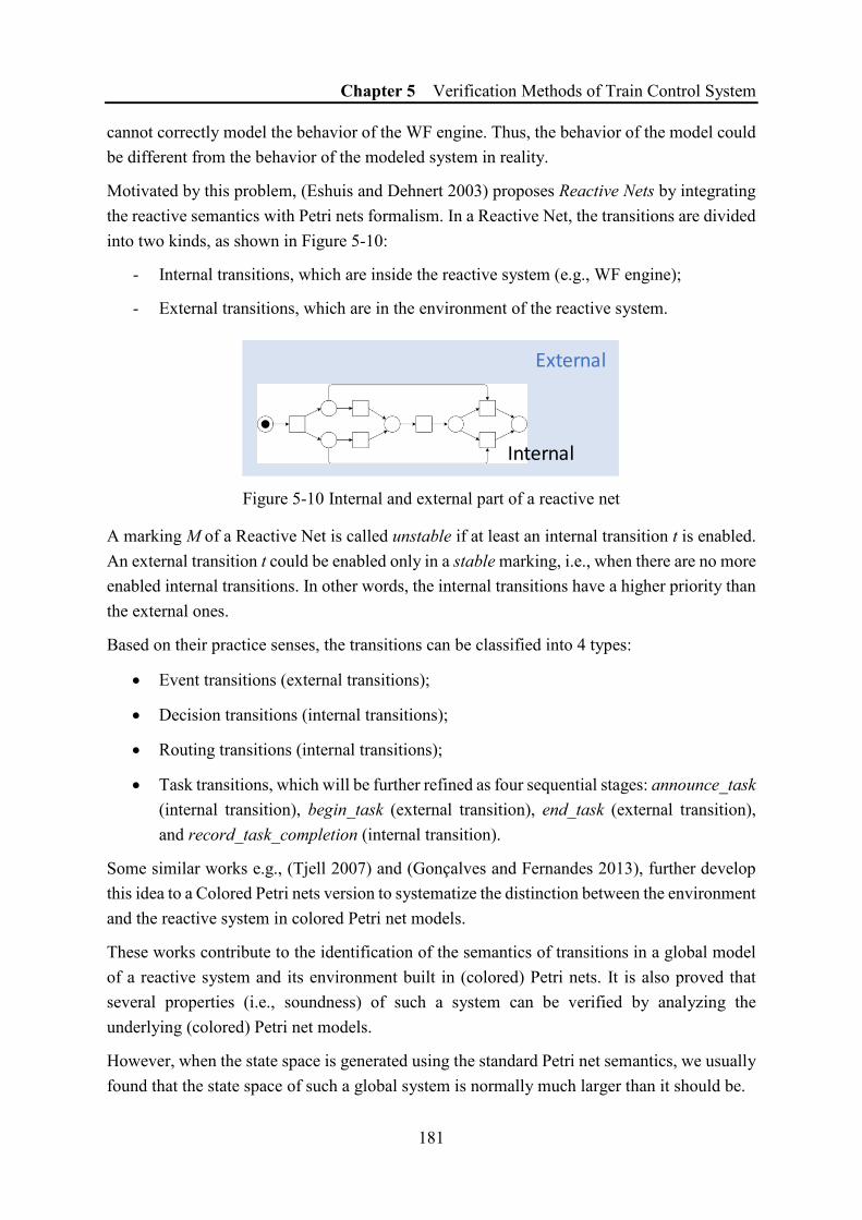
Chapter 5 Verification Methods of Train Control System
181
cannot correctly model the behavior of the WF engine. Thus, the behavior of the model could be different from the behavior of the modeled system in reality.
Motivated by this problem, (Eshuis and Dehnert 2003) proposes Reactive Nets by integrating the reactive semantics with Petri nets formalism. In a Reactive Net, the transitions are divided into two kinds, as shown in Figure 5-10:
- Internal transitions, which are inside the reactive system (e.g., WF engine);
- External transitions, which are in the environment of the reactive system.
Figure 5-10 Internal and external part of a reactive net
A marking M of a Reactive Net is called unstable if at least an internal transition t is enabled. An external transition t could be enabled only in a stable marking, i.e., when there are no more enabled internal transitions. In other words, the internal transitions have a higher priority than the external ones.
Based on their practice senses, the transitions can be classified into 4 types:
• Event transitions (external transitions);
• Decision transitions (internal transitions);
• Routing transitions (internal transitions);
• Task transitions, which will be further refined as four sequential stages: announce_task (internal transition), begin_task (external transition), end_task (external transition), and record_task_completion (internal transition).
Some similar works e.g., (Tjell 2007) and (Gonçalves and Fernandes 2013), further develop this idea to a Colored Petri nets version to systematize the distinction between the environment and the reactive system in colored Petri net models.
These works contribute to the identification of the semantics of transitions in a global model of a reactive system and its environment built in (colored) Petri nets. It is also proved that several properties (i.e., soundness) of such a system can be verified by analyzing the underlying (colored) Petri net models.
However, when the state space is generated using the standard Petri net semantics, we usually found that the state space of such a global system is normally much larger than it should be.
External
Internal

Chapter 5 Verification Methods of Train Control System
182
In this thesis, we exploit the reactive semantics in a global railway control system model to reduce the unnecessary states caused by the concurrence of different components and the environment. This idea will be introduced in the following subsections.
5.4.2 Global System Composed of Multiple Reactive Components
We consider a practical case that a global system is made of multiple components and the environment, where each component is a reactive system and it can interact with the environment. In this thesis, we call such a component that has the reactive semantics a reactive component. Figure 5-11 illustrates a global system with two reactive components.
Figure 5-11 Global system made of multiple reactive components
The application of such a global system configuration is very common in control systems. Taking the MA management function in the ETCS as an example, two reactive components could be the onboard system (which requests and receives MAs) and the RBC (which generates MAs based on the MA requests); the transitions in the environment could be the changes in the train position (e.g., the reception of the telegram from a new balise for location purpose).
It is obvious that in this example, the internal transitions of the two should use reactive semantics. For the onboard system component, once the condition to request a new MA is satisfied, it should be executed immediately to maintain the continuous advancement of the train. For the RBC component, when an MA request is received, the generation of a new MA also should be processed as soon as possible to keep the functionality. While the transitions of train advancement in the environment should have the standard token-game semantics because they represent in fact the events and the occasions that they are fired are not controllable in such a system.
Essentially, the distinction between the two semantics of different transitions stands for two priority levels of the transitions. As said in (Westergaard and Verbeek 2011), high-priority transitions can be used to model exception handling and low-priority transitions can be used to model background tasks that should only be executed when no other transition is enabled.
Environment
Component A Component B
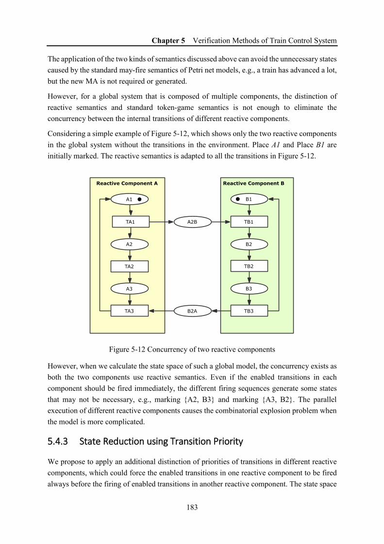
Chapter 5 Verification Methods of Train Control System
183
The application of the two kinds of semantics discussed above can avoid the unnecessary states caused by the standard may-fire semantics of Petri net models, e.g., a train has advanced a lot, but the new MA is not required or generated.
However, for a global system that is composed of multiple components, the distinction of reactive semantics and standard token-game semantics is not enough to eliminate the concurrency between the internal transitions of different reactive components.
Considering a simple example of Figure 5-12, which shows only the two reactive components in the global system without the transitions in the environment. Place A1 and Place B1 are initially marked. The reactive semantics is adapted to all the transitions in Figure 5-12.
Figure 5-12 Concurrency of two reactive components
However, when we calculate the state space of such a global model, the concurrency exists as both the two components use reactive semantics. Even if the enabled transitions in each component should be fired immediately, the different firing sequences generate some states that may not be necessary, e.g., marking {A2, B3} and marking {A3, B2}. The parallel execution of different reactive components causes the combinatorial explosion problem when the model is more complicated.
5.4.3 State Reduction using Transition Priority
We propose to apply an additional distinction of priorities of transitions in different reactive components, which could force the enabled transitions in one reactive component to be fired always before the firing of enabled transitions in another reactive component. The state space
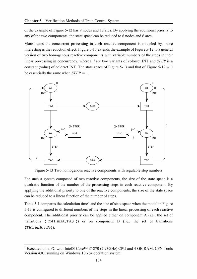
Chapter 5 Verification Methods of Train Control System
184
of the example of Figure 5-12 has 9 nodes and 12 arcs. By applying the additional priority to any of the two components, the state space can be reduced to 6 nodes and 6 arcs.
More states the concurrent processing in each reactive component is modeled by, more interesting is the reduction effect. Figure 5-13 extends the example of Figure 5-12 to a general version of two homogenous reactive components with variable numbers of the steps in their linear processing in concurrency, where 𝑇𝑇, 𝑗𝑗 are two variants of colorset INT and 𝑆𝑆𝑇𝑇𝐸𝐸𝐶𝐶 is a constant (value) of colorset INT. The state space of Figure 5-13 and that of Figure 5-12 will be essentially the same when 𝑆𝑆𝑇𝑇𝐸𝐸𝐶𝐶 = 1.
Figure 5-13 Two homogenous reactive components with regulable step numbers
For such a system composed of two reactive components, the size of the state space is a quadratic function of the number of the processing steps in each reactive component. By applying the additional priority to one of the reactive components, the size of the state space can be reduced to a linear function of the number of steps.
Table 5-1 compares the calculation time* and the size of state space when the model in Figure 5-13 is configured to different numbers of the steps in the linear processing of each reactive component. The additional priority can be applied either on component A (i.e., the set of transitions { 𝑇𝑇𝐴𝐴1, 𝑇𝑇𝑇𝑇𝑠𝑠𝐴𝐴, 𝑇𝑇𝐴𝐴3 }) or on component B (i.e., the set of transitions {𝑇𝑇𝐵𝐵1, 𝑇𝑇𝑇𝑇𝑠𝑠𝐵𝐵, 𝑇𝑇𝐵𝐵3}).
* Executed on a PC with Intel® Core™ i7-870 (2.93GHz) CPU and 4 GB RAM, CPN Tools Version 4.0.1 running on Windows 10 x64 operation system.

Chapter 5 Verification Methods of Train Control System
185
For such a system composed of two reactive components, the size of the state space is a quadratic function of the number of the processing steps in each reactive component. By applying the additional priority to one of the reactive components, the size of the state space can be reduced to a linear function of the number of steps.
Table 5-1 Comparison of state spaces with/without additional priority
STEP (𝑠𝑠) Without additional priority With additional priority (on A or B)
Cal. Time Nodes No. Arcs No. Cal. Time Nodes No. Arcs No.
1 5s 9 12 4s 6 6
10 6s 144 264 5s 24 24
100 10s 10404 20604 6s 204 204
200 48s 40804 81204 6s 404 404
𝐹𝐹(𝑠𝑠) - 𝑠𝑠2 + 4𝑠𝑠 + 4 2𝑠𝑠2 + 6𝑠𝑠 + 4 - 2𝑠𝑠 + 4 2𝑠𝑠
For a global system composed of multiple reactive components and environment, the reduction method can be applied by defining different levels of priority for the transitions in different reactive components, as shown in Figure 5-14.
Figure 5-14 Semantics and transition priority in a global system
This reduction technique is effective when the state space explosion is caused by the concurrence of the inner states of different reactive components. We explain the application rules of this reduction technique.
The reduction technique can be applied to a (colored) Petri net model of a global system composed of different reactive components and the environment. A reactive component should not contain external transitions (e.g., event transitions), which can only appear in the environment.
Environment (Transitions are of lowest priority)
Component 1(Priority 1
higher) Component 2(Priority 2)
Component N(Priority N -
lower)
…Reactive
Semantics
Token-game Semantics

Chapter 5 Verification Methods of Train Control System
186
The reactive components are interleaving in a manner that they are “reactive” to (or “driven” by) the tokens in the concerned interface places between them and the environment. For a particular component, the changes occurred in the interface places, e.g., the presence of new tokens, can be regarded as an input which turns some transitions in the reactive component enabled. Then, the reactive component executes the processing steps until no more transitions are enabled. As a result, it usually produces some changes in some related interface places as an output. These changes are then used as input for another reactive component.
In terms of properties that can be verified, the application of this technique is based on the promise that the processing in each reactive component is rather independent, which means the combinations of the internal states in different reactive components is irrelevant to the desired system properties.
Particularly, this technique is not applicable to the modeling of the competition of resources by different reactive components where exists an uncertainty.
This technique is based on the analysis of the semantics of the transitions and takes advantage of the system modularity. It is implemented by assigning different priorities to the transitions in different reactive components. Compared to the other modular methods introduced in §5.3, the advantage of this method is that it allows the verification of the properties about the whole system using the reduced but global state space. In other words, it does not require the decomposition (which could be very difficult) of the desired properties or the state space.
In terms of implementation of the reactive semantics and the transition priorities, CPN Tools supports the prioritized transitions (Guan et al. 1998; Westergaard and Verbeek 2011), which have been introduced in §4.4.2.3.
5.5 Case Study: Verification of Mode Transitions
Mode transitions are an important function in the modeling of ETCS onboard system (see §4.4.1). A set of various properties can be verified on the model of mode transitions in §B.1.2.
We propose to verify the ETCS mode transitions function in two ways:
- In an isolated way: we isolate the mode transitions model by setting all the mode transition conditions to “true” (or by removing all the conditions) and by unifying all the transitions to the same priority. Thus, we can generate a reachability graph of the mode transitions model indicating all the possibilities of mode transitions, which is especially useful for the verification of reachability properties.
- In a global way with a scenario: the mode transitions model with conditions and priorities is needed, as well as the necessary models to execute a scenario. It is useful to verify the user-specified properties about the mode transitions during the execution of the scenario, some examples are shown below.

Chapter 5 Verification Methods of Train Control System
187
5.5.1 Verification of Mode Transitions in an Isolated Way
The state space of the isolated mode transitions model considering 12 modes (considered modes: NP, SB, PS, SH, FS, SR, OS, NL, SF, IS, RV, PT; not-considered modes: LS, SL, UN, TR, SN) is shown in Figure 5-15.
Figure 5-15 State space of isolated mode transitions model
Boundedness Verification
According to the ETCS system requirements specification, at any time (even if the equipment is not powered), the onboard system must be in one and only one mode. This requirement can be transformed into the boundedness verification of the place “Current_Mode”, in which the token indicates the current ETCS mode.
The boundedness property is one of the standard Petri nets properties, which can be found in the state space report generated by CPN Tools. It can also be checked by using two pre-defined functions “UpperInteger ()” and “LowerInteger ()”, as shown in Code 5-2
Code 5-2 Model checking of the boundedness using pre-defined functions 01 val ModeUpperBound= UpperInteger (Mark.Mode_Transitions'Current_Mode
1) ; 02 val ModeLowerBound = LowerInteger (Mark.Mode_Transitions'Current_Mode
1) ; 03 val Result = (ModeUpperBound=1) andalso (ModeLowerBound=1);

Chapter 5 Verification Methods of Train Control System
188
Reachability Verification
As a basic Petri net property, the reachability of two nodes can be checked by using the pre-defined function “Reachable ()” or its chatty version “Reachable’ ()” which also returns a text explanation about the (shortest path), as shown in Figure 5-16.
Figure 5-16 Model checking of reachability using a pre-defined function
The reachability property can also be checked by evaluating an ASK-CTL expression.
For example, Code 5-3 checks if it is possible from the initial marking, where the current mode is “NP” (No Power), to reach a marking where the mode is “PT” (Post Trip).
Code 5-3 Model checking of reachability using ASK-CTL 01 fun IsInModePT n = (Mark.Mode_Transitions'Current_Mode 1 n = 1`SF); 02 val myASKCTLformula = POS (NF ("In Mode PT", IsInModePT)); 03 eval_node myASKCTLformula InitNode;
The first line defines a function whose argument is a node in the state space and returns a Boolean value to indicate whether the current mode in this state is “SF”. The ASK-CTL expression uses the operator “POS” (POSsible), which means that a future state which satisfies its argument is reachable from the state where we evaluate the expression. The function “NF” will be explained later.
The result of the verification is false. In fact, mode PT can only be entered from the mode “TR” (Trip). As the mode TR is currently not considered in the mode transitions model, it is rational that a state, where the mode is PT, is unreachable whatever the initial mode.
Dead marking
The ETCS requirements specification says, “to leave Isolation (IS) mode, a special operation procedure is needed”, which means “no transition from Isolation mode is specified”. In the Petri net model, it means that a node representing the system in Mode IS should be a dead marking.
Using ASK-CTL model checking, the dead marking property can be checked by using “MODAL” operator, which checks the existence of immediate transitions of a node (marking), as shown in Code 5-4.

Chapter 5 Verification Methods of Train Control System
189
Code 5-4 Model checking of dead marking using ASK-CTL 01 val IsInModeIS n = Mark.Mode_Transitions'Current_Mode 1 n = 1`IS; 02 (* In the example node 2 is in Mode IS*) 03 IsInModeIS 2; 04 val IsDeadMarking = NOT ( MODAL ( TT ); 05 eval_node IsDeadMarking 2;
After having acquired the information that the node 2 is in Mode IS, another way to execute the model checking verification is to use the pre-defined functions “fun DeadMarking : Node -> bool” or “fun Terminal : Node -> bool”, as shown in Figure 5-17.
Figure 5-17 Model checking of dead marking using pre-defined function (Terminal)
The result shows that the node 2 in the state space (the system in Mode IS) is a dead marking.
User-specified property of the switch to SF mode
The system designer can use the pre-defined functions in CPN Tools and ASK-CTL formulas to check more complicated properties. In order to give an example, we verify the switch from other modes to System Failure (SF) mode.
In any working mode (all the ETCS modes except for IS, NP, SL, NL, SF), when the system detects a failure, the ETCS onboard system will switch immediately to SF mode, which assures the safety (as in SF mode the onboard equipment permanently executes the emergency brakes). This property can be checked by a property written using ASK-CTL as shown in Code 5-5.
Code 5-5 Model checking of reachability using ASK-CTL 01 fun GetMode n = Mark.Mode_Transitions'Current_Mode 1 n; 02 fun IsInModeSF n = (GetMode n = 1`SF); 03 fun IsNoWorking n = (GetMode n = 1`IS) orelse (GetMode n = 1`NP)
orelse (GetMode n = 1`SL) orelse (GetMode n = 1`NL) orelse (IsInModeSF n);
04 val PredSF= NF ("In Mode SF", IsInModeSF); 05 val PredNoWorking = NF ("In Mode IS or NP or SL or NL or SF",
IsNoWorking); 06 val myASKCTLformula = INV (OR (PredNoWorking, EXIST_NEXT (PredSF)); 07 eval_node myASKCTLformula InitNode;
The first three lines define several functions to get and classify the mode value. The fourth and the fifth lines define two atomic predicates using the NF function (val NF: string * (Node -> bool) -> A), which in fact transforms a function of the type “Node -> bool” to an ASK-CTL “state formulas (𝒜𝒜)”. There exists correspondingly another function AF (val
Chapter 5 Verification Methods of Train Control System
190
AF: string * (Arc -> bool) -> B) which transforms a function of the type “Arc -> bool” to an ASK-CTL “transition formulas (ℬ)”.
The sixth line specifies the ASK-CTL formula to check. “INV” (short for “invariant”) is a derived path quantification operator. When used as a state formula, “INV (𝒜𝒜)” is true iff its argument ( 𝒜𝒜 ) is always true for all the reachable states from the state we are now. “EXIST_NEXT” is an immediate successor operator. The expression “myASKCTLformula” in Code 5-5 means that for all the reachable states, if a state is not in one of the NoWorking modes, it shall have the possibility to be switched to SF mode immediately (in case a failure is detected). The last line evaluates this expression on the initial state.
The result is true, which shows that the desired property is verified.
5.5.2 Verification of Safety Property in a Global Way with a Scenario
Safety-related properties usually mean the searching of some dangerous states in all the possible states of a system. In order to conduct the safety verification on the actual operation situation of the ETCS onboard system, it is necessary to combine the models of mode transitions, procedures, onboard functions, etc., as introduced in §4.4.
We are interested in a safety-related property about the certainty of (onboard) mode transition, which is, at any moment, the ETCS onboard system cannot have more than one possibility to switch to another mode. In other words, if the onboard system is ready to switch to another mode, the future mode should be unique. This requirement has been discussed from the modeling point of view in §4.4.2.3. In this case study, we propose to verify this requirement using compositional verification.
Formally, we present the Mode Transitions Table (Table B-1 in Appendix A) as a set 𝑀𝑀𝑇𝑇𝑇𝑇 of mode transitions. A mode transition 𝑚𝑚𝑡𝑡 ∈ 𝑀𝑀𝑇𝑇𝑇𝑇 is a 4-tuple structure 𝑚𝑚𝑡𝑡 =< 𝑚𝑚𝐵𝐵, 𝑚𝑚𝑆𝑆, 𝑇𝑇, 𝐶𝐶 >, where:
- 𝑚𝑚𝐵𝐵 is the origin mode, 𝑚𝑚𝐵𝐵 ∈ 𝑀𝑀 the set of all the modes;
- 𝑚𝑚𝑆𝑆 is the target mode, 𝑚𝑚𝑆𝑆 ∈ 𝑀𝑀;
- 𝑇𝑇 is the priority value, 𝑇𝑇 ∈ 𝐶𝐶 = {𝑇𝑇1, 𝑇𝑇2, … , 𝑇𝑇7};
- 𝐶𝐶 is a condition 𝑐𝑐 ∈ 𝐶𝐶 (𝐶𝐶 is the set of conditions) that is necessary to enable the mode transition 𝑚𝑚𝑡𝑡.
The desired property 𝜑𝜑 is specified as 𝜑𝜑: ∀𝑚𝑚0 ≠ 𝑚𝑚1 ≠ 𝑚𝑚2, there should not have a reachable marking 𝑀𝑀 ∈ ℛ(M0) that enables two different mode transitions 𝑚𝑚𝑡𝑡′ = {𝑚𝑚0, 𝑚𝑚1, 𝑇𝑇′, 𝑐𝑐′} and 𝑚𝑚𝑡𝑡′′ = {𝑚𝑚0, 𝑚𝑚2, 𝑇𝑇′′, 𝑐𝑐′′}.

Chapter 5 Verification Methods of Train Control System
191
We applicate the compositional verification method to separate the property 𝜑𝜑 into two sub properties 𝜑𝜑� and 𝜑𝜑�:
- 𝜑𝜑� : ∀𝑚𝑚0 ≠ 𝑚𝑚1 ≠ 𝑚𝑚2 , and 𝑇𝑇′ ≠ 𝑇𝑇′′ , two different mode transitions 𝑚𝑚𝑡𝑡′ =
{𝑚𝑚0, 𝑚𝑚1, 𝑇𝑇′, 𝑐𝑐′} and 𝑚𝑚𝑡𝑡′′ = {𝑚𝑚0, 𝑚𝑚2, 𝑇𝑇′′, 𝑐𝑐′′} are not able to be enabled at the same time;
- 𝜑𝜑�: ∀𝑚𝑚0 ≠ 𝑚𝑚1 ≠ 𝑚𝑚2, if there exists two mode transitions 𝑚𝑚𝑡𝑡′ = {𝑚𝑚0, 𝑚𝑚1, 𝑇𝑇, 𝑐𝑐′} and
𝑚𝑚𝑡𝑡′′ = {𝑚𝑚0, 𝑚𝑚2, 𝑇𝑇, 𝑐𝑐′′} where 𝑚𝑚0 ≠ 𝑚𝑚1 ≠ 𝑚𝑚2 , there exists not a marking 𝑀𝑀 ∈ℛ(M0) that satisfies both 𝑐𝑐′ and 𝑐𝑐′′.
𝜑𝜑� can be verified by the isolated Mode Transitions model easily. In fact, the modeling formalism of Petri nets with prioritized transitions (see Figure 4-18) already ensures this property.
𝜑𝜑� needs to be verified via a traversal on the global state space of a global system. However, an actual operation of the ETCS onboard system depends on a lot of interactions with other systems and the driver’s choices. In order to generate part of the state space of the onboard system, we consider the procedure “Start of Mission (SoM)” (see B.2) and we create an operation scenario which allows the onboard system to execute the following operations:
𝑀𝑀𝐵𝐵𝑆𝑆𝑇𝑇 𝑁𝑁𝐶𝐶 → 𝑀𝑀𝐵𝐵𝑆𝑆𝑇𝑇 𝑆𝑆𝐵𝐵 ��������� ��� ����������→ 𝑀𝑀𝐵𝐵𝑆𝑆𝑇𝑇 𝑆𝑆𝑆𝑆 (5-7)
The operation scenario for the procedure SoM is defined by two parts:
- The initial operation states corresponding to the initial mode NP;
- The necessary interactions during the execution of the scenario, an example is shown in Figure 5-18.
Figure 5-18 Example of the scenario in procedure SoM
The scenario is executed on a combination of the complete model of mode transitions, the model of procedure SoM and the models of concerned onboard functions.

Chapter 5 Verification Methods of Train Control System
192
In order to verify the property 𝜑𝜑� in this example scenario where 𝑚𝑚0 = 𝑆𝑆𝐵𝐵 (in procedure
SoM), all the possible combinations of 𝑚𝑚𝑡𝑡′ = {𝑚𝑚0, 𝑚𝑚1, 𝑇𝑇, 𝑐𝑐′} and 𝑚𝑚𝑡𝑡′′ = {𝑚𝑚0, 𝑚𝑚2, 𝑇𝑇, 𝑐𝑐′′} need to be verified.
Figure 5-19 shows the possibility to verify that for 𝑚𝑚𝑡𝑡′ = {𝑚𝑚0 = 𝑆𝑆𝐵𝐵, 𝑚𝑚1 = 𝑁𝑁𝑆𝑆, 𝑇𝑇 = 𝑇𝑇7, 𝑐𝑐′ =𝐶𝐶70} and 𝑚𝑚𝑡𝑡′′ = {𝑚𝑚0 = 𝑆𝑆𝐵𝐵, 𝑚𝑚2 = 𝑀𝑀𝑆𝑆, 𝑇𝑇 = 𝑇𝑇7, 𝑐𝑐′′ = 𝐶𝐶15}. The result shows that no markings in this scenario allows the two conditions C70 (“Show LS Proposal”) and C15 (“Show OS Proposal”) to be satisfied simultaneously.
Figure 5-19 Verification of Mode Transition Model
In Figure 5-19 the function CalculateOccGraph is used to generate the state space and the function SearchNodes is used to traverse the nodes of the state space. The details about these functions can be referred to (University of Aarhus 2006).
This verification can also be executed on-the-fly if the size of the state space generated by the scenario is important. In CPN Tools, a predicate of type (fn n => bool) in the StopOptions can be set for to automatically stop the state space generation. We have shown the methods to verify the property φq in a scenario. It can be used together with φp to infer the property φ about the global system in a compositional way.
Code 5-6 shows the configuration for the state space generation with the on-the-fly verification for the same verification objective above. In the example, the option Secs is set to 300s to avoid a too long waiting time caused by errors. If the size of the state space is expected to be longer, the option can be altered.
We have shown the methods to verify the property 𝜑𝜑� in a scenario. It can be used together
with 𝜑𝜑� to infer the property 𝜑𝜑 about the global system in a compositional way.

Chapter 5 Verification Methods of Train Control System
193
Code 5-6 Model checking with ASK-CTL formula 01 fun shown_LS_Proposal n = Mark.Mode_Transitions'LS_Proposal 1 <> []; 02 fun shown_OS_Proposal n = Mark.Mode_Transitions'OS_Proposal 1 <> []; 03 OGSet.StopOptions{ 04 Nodes = NoLimit, 05 Arcs = NoLimit, 06 Secs = 300, 07 Predicate = (fn n => shown_LS_Proposal andalso shown_OS_Proposal)}; 08 CalculateOccGraph;
However, it can be predicted that the assertion “two mode transition conditions with the same priority will never be satisfied simultaneously” (i.e., the property 𝜑𝜑�) would be very difficult even not feasible as it requires the generation of a state space that covers all the possible system operation states. In terms of the system testing, there are studies about the automatic generation of test sequences based on test cases to provide a best test coverage (Zhang et al. 2014), but it is still far from the requirement to formally cover all the possible operation states.
Thus, from the point of view of redaction of the system requirements specification, we would personally suggest using more rigorous constraints for the mode transition rules, i.e., the assignment of a unique priority to each mode transition with the same origin mode and without syntactically contradictory conditions. The proposition will not change the desired behavior of the train control system but can avoid some design errors in a very early phase.
5.6 Case Study: Verification of MA Function using
Assume-Guarantee
5.6.1 Background of the Case Study and the desired Property
The case study applies the assume-guarantee reasoning to verify the MA function in a railway system, i.e., an RBC with multiple trains. The case study considers the train model of MA function presented in (Xie et al. 2017a) and the RBC model in Figure 4-39.
We recall some modeling assumptions of the MA function:
(1) Each time a train enters in a new block, we assume that it receives its current position from a Eurobalise and then sends a position report to the corresponding RBC, instead of considering the specified report format according to ERTMS/ETCS-2 standard.
(2) Once the RBC receives the position report from a train, it updates its location in the database. The RBC also considers the location report as an MA request (see Place Request in Figure 4-39). Consequently, it generates MA for the train that just advanced.
Chapter 5 Verification Methods of Train Control System
194
The verification to conduct is a classical test in the railway control system: a train follows another train to advance.
The objective of verifying this property is twofold. On the one hand, the property implies the safety (collision-free) that the follower train will never run into its predecessor. On the other hand, if the follower train can always follow the predecessor train to stop and to advance, it can partially verify the correctness of the train operation regulated by MA.
This property is quite difficult to be verified due to the following complex reasons:
(1) In this thesis, we propose to model the RBC module in WFN while the train module is modeled using CPN enhanced with CPN Tools. The heterogeneity of the different modeling formalisms could be an obstacle to generate the global state space;
(2) The MA generation function in the RBC part needs to consider the state (position) of other trains. The RBC model interactives with each train and uses the centralized storage for the positions of all the trains (see §4.6). It is thus very difficult to isolate the RBC model to generate an independent state space.
We propose to use the assume-guarantee reasoning to verify the property.
5.6.2 Environment Abstraction using Assume-Guarantee
The desired property is to verify that a follower train can “follows” its predecessor train, which means, it stops if the predecessor train stops and it can restart after the predecessor train advances.
The verification will be focused on the follower train (i.e., the train behind) and considers all the other parts in the global system as its environment, including the RBC and the predecessor train.
In order to better present the verification in the thesis, we consider a simple railway line composed of only five blocks, managed by an RBC.
We assume that the environment of the follower train behaves in this order:
(1) Initially, the follower train is in Block 1 and the predecessor train is in Block 4;
(2) The follower train has advanced but the predecessor train is at standstill in Block 4;
(3) During the duration that the follower train is in Block 3, the predecessor train advances, passes Block 4 and Block 5, and leaves this railway line.
Using the assume-guarantee reasoning expressed in (5-6), the considered follower train model is denoted by 𝑀𝑀, its environment is denoted by 𝑀𝑀′, and the assumed environment behavior is denoted by 𝜓𝜓.
Now we focus on the verification of the expression ⟨𝜓𝜓⟩ 𝑀𝑀 ⟨𝜑𝜑⟩ on follower train model M.

Chapter 5 Verification Methods of Train Control System
195
The assumption 𝜓𝜓 is implemented via some extra models built in CPN Tools, which is attached with the train model. In order to conduct the verification, we also need the information from the Balise to represent the advancement of the follower train in the railway lines. Thus, the environment of the follower train also includes an abstracted model of Balise to send the positioning Balise telegrams.
As a result, two abstracted models are attached to the train model, as shown in Figure 5-20.
Figure 5-20 Abstraction of the train’s environment
5.6.2.1 Abstraction of Balise
As the Balises are out of the scope of the train controller, they are not considered in our models. To verify the functions of train controller, the corresponding balise messages should be regularly sent to the interface place of balise (Place Balise in Figure 5-20 or Places TxBTM in Figure 4-9).
The left part of Figure 5-20 simulates the behaviors of Balises. We use Time Stamp in CPN Tools to control the time interval of Balise message generation.
If the condition [EOA>POS] is satisfied, a new token representing Balise message will be generated and put into Place Balise, with value = POS+1 where POS is the current block that the train is occupying.
5.6.2.2 Abstraction of RBC and the predecessor train
Based on the analysis of the environment’s behavior at the beginning of §5.6.2, we use a single transition with its necessary auxiliary parts (e.g., some places and functions) as a simplification of the RBC component as shown in the right part of Figure 5-20.
The functions of this abstracted RBC model are:
Position
POS 1`1
EOA
POS
1
TrainIn/Out TID
1`T(1)
T2RBC
TypexTIDxPOS
RBC2T
TypexTIDxPOS
BaliseIn POS
Registered
BOOL
1`false
Delay
UT
()@1 TIDComm
TID
1`T(1) History
INT
1
Advance
[pos
<>
1]
ReceiveMA
Disconnect
Register
NextBlock
[eoa
>
pos]AbsRBC
(UPDATE,tid,pos)
(MAMSG,tid,neoa)
neoa
tpos
tid
N(REMOVE,tid,N)
(INSERT,tid,1)
false
true
false
true true
()@+5
()
pos+1
pos
tid
tid
tid
(tp,tid,pos)
if (tp=MAMSG)then (MAMSG, tid,if (i
<
=3) then 3 else 5)else (tp,tid,pos)
tid
eoa
1
if (tp=MAMSG)then (i+1) else i
i
pos
pos
eoa
pos
pos
WAck
TypexTID
(UPDATE,tid)
(REMOVE,tid)
(INSERT,tid)
In
In/Out
Abstraction of Balise
Abstraction of RBC and the
predecessor train

Chapter 5 Verification Methods of Train Control System
196
- For the first three position reports (regarded as MA requests) received from the follower train (sent in Block 1, 2 and 3), the RBC provides the train with the MA whose EOA=3 (since the predecessor train is on block 4);
- For the future position reports / MA requests sent by the follower train (if there are), the RBC shall provide the train with an MA whose EOA=5 (since the predecessor train has left).
5.6.3 Verification of Train Model using Assume-Guarantee
After the assumption 𝜓𝜓 is implemented by the abstracted models, the expression ⟨𝜓𝜓⟩ 𝑀𝑀 ⟨𝜑𝜑⟩ can be verified by analyzing the train model together with the two attached parts.
The state space of such a model is easily generated. A simplified version (after the aggregation of some linear states to achieve a compact representation) is presented in Figure 5-21.
Figure 5-21 State space of the train model under the assumption
Obviously, Node 11 in the state space represents an unexpected deadlock marking. This dead marking indicates that after the follower train arrives at EOA position (POS=EOA=3), it cannot advance anymore.
Even though the situation could be regarded to be “safe”, it does not totally satisfy the desired property. With our assumption, after the follower train enters Block 3 and its predecessor train has gone, the RBC is ready to provide the follower train with extended MA whose EOA=5.
By using the state space analysis method, we can conclude that the behavior of the train model under the aforementioned assumptions does not satisfy the desired property. It is even not necessary to verify the assumption about the environment ⟨𝑡𝑡𝑉𝑉𝑡𝑡𝑇𝑇⟩ 𝑀𝑀′ ⟨𝜓𝜓⟩.
5.6.4 Discussion of the Verification Result and Improvement
In this case study, we have found a design defect in the models presented in our previous work (Xie et al. 2017a). After the analysis, the problem is due to a combination of the two factors:

Chapter 5 Verification Methods of Train Control System
197
(1) For simplification reason, the train model does not send explicit MA request. The request of new MA is implicit by the position report. For this reason, once the train stops, it loses the ability to require a new MA;
(2) The strategy that RBC replies an MA request: the RBC module replies the train immediately even if the new EOA is the end position of the current Block occupied by the train, which has no sense for the MA update of the onboard system. After this “update” the train requires no more MA even if the RBC might be able to extend it.
The solution could be to separate the MA request and the position report, and the request of MA should be executed periodically even if the train is at standstill. In the modeling of ETCS onboard system in §4.4 of this thesis, the requirement “Request MA Cyclically respect to approach of target indication point or MA timer elapsing” has been taken into consideration. Thus, the problem should not appear.
5.7 Conclusion of Chapter 5
This chapter deals with the verification of the colored Petri nets models of the train control systems built following the methodology presented in Chapter 4.
In this chapter, we first review the possible techniques to verify the Petri net model of a complex DES, among which the model checking technique is most commonly used. As an important of the verification, the property specification is also discussed.
To fight the famous combinatorial explosion problem, we introduce both some efficient state space analysis techniques and several modular verification methods. These approaches can reduce the state space on two levels and may be applied together to achieve the result.
Faced with the difficulty of verifying the global system model of train control, we are inspired by the reactive semantics which was first introduced in reactive nets. We identify the reactive components in a global system and propose to reduce the global state space based on reactive semantics and transition priority. This technique can be used in similar complex DES.
We also summarize the case studies introduced in this chapter in Table 5-2
Table 5-2 Case studies in Chapter 5
Case study Property State Space Technique Modular Method
§5.5.1 Standard, User-specified ASK-CTL, CPN Tools pre-defined functions
-
§5.5.2 User-specified On-the-fly Compositional
§5.6 Safety, User-specified State space exploration Assume-guarantee


199
Chapter 6 CONCLUSIONS OF THE THESIS AND PERSPECTIVES
6.1 Conclusions
This thesis deals with the formal modeling and verification of complex train control systems using colored Petri nets, as an example of complex Discrete Event Systems (DES).
The most important problem in the development of complex DES is the combinatorial explosion, which exists both in the modeling stage and the verification stage due to the huge number of states. The alleviation of this problem can be proposed on several levels:
• Technical level
• Methodological level
• Level of application domains
This thesis exploits the three kinds of propositions in order to obtain efficient modeling and verification approaches, taking train control systems as an example.
The contributions of this thesis are threefold:
(1) This thesis synthesizes the modeling and verification formalisms in literature and proposes a methodology of modeling and verification for train control systems. The methodology offers the possibility to model and verify a global train control system using colored Petri nets (CPN) in a modular way, in order to reduce the complexity.
(2) Faced with some difficulties, we propose some techniques that can be regarded as the general technical contributions of the development of complex DES. In the modeling stage, we propose several modeling patterns of well-formed Petri nets (WFN) to facilitate the modeling using this formalism; in the verification stage, we analyze the reactive semantics and the transition priority of a global system composed of multiple reactive components and propose a technique to reduce the system states.
(3) From an industrial point of view, this thesis has produced several practical CPN models compatible with the latest standards of the European Train Control System (ETCS). These models can be used as modeling bricks in the projects (e.g., UniRAIL in Centrale Lille) for different modeling and analysis objectives.
The structure of this thesis is shown in Figure 6-1.

Chapter 6 Conclusions of the Thesis and Perspectives
200
Figure 6-1 Structure of this manuscript
6.2 Perspectives
In terms of the improvement of this work, we would like to point out the following perspectives:
(1) The modeling stage and the verification stage in this thesis study are somehow “separated”, which results in some inconvenience in the downstream stage – verification stage. From a global point of view, the modeling stage and the verification stage might be better coordinated to facilitate the verification of desired properties. Particularly, incremental approaches in both modeling and verification stages should be emphasized, which might facilitate the verification to some extent.
Chapter 1Introduction
Motivations / Objectives
Chapter 2Application Framework:
Railway Systems and Train ControlEmphasis on ERTMS/ETCS
Chapter 3Theoretical Framework:
Complex DES Development FormalismsEmphasis on Colored Petri nets
Chapter 4Modular Modeling of Train Control Systems
- Systematical modeling methodology for train control systems;- Structural modeling based on components in a whole railway system;- Functional modeling of ETCS onboard equipment;- Modeling of Railway node with automated routing using CPN Tools;- Modeling of RBC with MA management function using WFN;- Proposition of general modeling patterns in WFN.
Chapter 5Verification Methods of Train Control Systems and Case Studies
- Review of verification techniques for colored Petri nets;- Review of modular verification approaches for complex DES;- Formal description of properties for colored Petri net models;- State reduction based on reactive semantics and transition priority;- Case studies of verification of railway control systems.
Chapter 6Conclusion and Perspectives

Chapter 6 Conclusions of the Thesis and Perspectives
201
(2) The verification presented in this thesis depends too much on state space methods, despite the potential of invariant analysis for Petri nets. The situation may result from the complexity to apply colored invariants and the limited support of properties for the verification. However, we believe that the colored invariant methods should be exploited either for the verification purpose or for the reduction purpose.
In terms of the whole lifecycle (Figure 1-1) of the complex DES development, we focus on the system design directly derived from the requirements specification and the verification. The extensions of this study are expected in the following aspects:
(1) Better lifecycle management of system development which clarifies different stages of requirements engineering, architecture design, and system design, etc. using model-driven engineering (MDE) and refinement-based approaches.
(2) Considering the implementation of control models, automatic code generation from Petri nets is quite necessary.
(3) Considering the practical need of testing the train control system before it is put into service (European Union Agency for Railways 2017), it would be useful to generate the test cases and test sequences from the control models.


203
Appendix A INTRODUCTION TO PETRI NETS Petri nets were invented by Carl Adam Petri in the 1960s (Petri 1962). It uses very simple syntax and structure to graphically present precise semantics, and is also a mathematical modeling and analysis tool (Murata 1989). Thanks to these features, Petri nets have been a popular formalism to model complex DES systems, especially for those with concurrency.
It is worth noting that the major contribution of Carl Adam Petri is not just a single modeling method (the initial model was the so-called Condition/Event nets, where the state is expressed in terms of Boolean variables), but the foundation of a set of net-based modeling formalisms within the “Petri nets” paradigm that have been developed over half a century (Silva 2012). All these formalisms are in the scope of “General Net Theory” founded by Carl Adam Petri (Petri 1980).
This appendix can be regarded as a complement of §3.3. It gives the reader an overview of the Petri nets theory and the most important Petri nets classes.
§A.1–§A.4 present some fundamental and famous Petri nets classes from a historical and developmental point of view. Each class is introduced with attention to its advancement and difference compared to its predecessors or analogs. A classification of these Petri nets variants can be found in §3.3.1.
§A.5 gives our explanation to a rather confusing situation of colored Petri net terminologies in the literature and clarifies the relevant definitions in this thesis.
§A.6 presents several Petri nets software, as a complement of §3.3.2.4 and §3.3.3.4.
A.1 Place/Transition-nets
Among the different Petri nets variants invented and still being developing by researchers, one of the most used and well-known types is the Place/Transition-nets (P/T-nets or PTN), which was defined in (Best and Fernández 1986). A P/T-net equipped with an initial marking constitutes a “Place/Transition (P/T) system” (Reisig 1986).
The Place/Transition-nets is such a fundamental class that it is also called classical/ordinary Petri nets, or just “Petri nets” in most of the literature.
Some important definitions of Place/Transition-nets are given as follows. Compared to how it was initially defined, we have slightly changed the expressive from in order to make it easier to understand.

APPENDIX A INTRODUCTION TO PETRI NETS
204
Definition A-1 A Place/Transition-net with initial marking is defined by a 5-tuple 𝐶𝐶𝑇𝑇𝑁𝑁 =(𝐶𝐶, 𝑇𝑇, 𝑊𝑊 −, 𝑊𝑊 +, 𝑚𝑚0) where:
• 𝐶𝐶 is the finite set of places;
• 𝑇𝑇 is the finite set of transitions, 𝐶𝐶 ∩ 𝑇𝑇 = ∅, 𝐶𝐶 ∪ 𝑇𝑇 = ∅;
• 𝑊𝑊 −: 𝐶𝐶 × 𝑇𝑇 → ℕ is the pre-incidence (or backward incidence) matrix that represents the integer weight from places to transitions;
• 𝑊𝑊 +: 𝐶𝐶 × 𝑇𝑇 → ℕ is the post-incidence (or forward incidence) matrix that represents the integer weight from transitions to places;
• 𝑚𝑚0 is an integer vector indexed by P and is called the initial marking (a marking is a particular state of a Petri net).
An example of Place/Transition-net can be found in Figure A-1.
Figure A-1 Place/Transition-net example
In this example, the set of places 𝐶𝐶 = {𝑇𝑇1, 𝑇𝑇2, 𝑇𝑇3, 𝑇𝑇4}, the set of transitions 𝑇𝑇 = {𝑡𝑡1, 𝑡𝑡2}, the pre-incidence matrix, the post-incidence matrix and the initial marking are respectively:
W− =
𝑡𝑡1 𝑡𝑡2𝑇𝑇1𝑇𝑇2𝑇𝑇3𝑇𝑇4 ⎣
⎢⎢⎡
1 00 10 20 1⎦
⎥⎥⎤, W+ =
𝑡𝑡1 𝑡𝑡2𝑇𝑇1𝑇𝑇2𝑇𝑇3𝑇𝑇4 ⎣
⎢⎢⎡
0 01 02 00 1⎦
⎥⎥⎤, 𝑚𝑚0 =
𝑇𝑇1𝑇𝑇2𝑇𝑇3𝑇𝑇4 ⎣
⎢⎢⎡
1001⎦
⎥⎥⎤
. (A-1)
Petri nets have not only a mathematical structural definition, but also a formal definition of their execution semantics.
Definition A-2 Let 𝐶𝐶𝑇𝑇𝑁𝑁 = (𝐶𝐶, 𝑇𝑇, 𝑊𝑊 −, 𝑊𝑊 +, 𝑚𝑚0) be a marked Place/Transition-net, then:
• 𝑡𝑡 ∈ 𝑇𝑇 is called firable from a marking m (denoted by “ 𝑚𝑚[𝑡𝑡⟩ ” iff ∀𝑇𝑇 ∈ 𝐶𝐶, 𝑚𝑚(𝑇𝑇) ≥𝑊𝑊 − (𝑇𝑇, 𝑡𝑡);
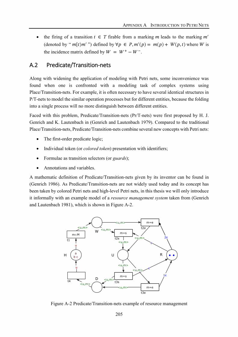
APPENDIX A INTRODUCTION TO PETRI NETS
205
• the firing of a transition 𝑡𝑡 ∈ 𝑇𝑇 firable from a marking 𝑚𝑚 leads to the marking 𝑚𝑚′ (denoted by “ 𝑚𝑚[𝑡𝑡⟩𝑚𝑚′ ”) defined by ∀𝑇𝑇 ∈ 𝐶𝐶, 𝑚𝑚′(𝑇𝑇) = 𝑚𝑚(𝑇𝑇) + 𝑊𝑊(𝑇𝑇, 𝑡𝑡) where 𝑊𝑊 is the incidence matrix defined by 𝑊𝑊 = 𝑊𝑊 + − 𝑊𝑊 −.
A.2 Predicate/Transition-nets
Along with widening the application of modeling with Petri nets, some inconvenience was found when one is confronted with a modeling task of complex systems using Place/Transition-nets. For example, it is often necessary to have several identical structures in P/T-nets to model the similar operation processes but for different entities, because the folding into a single process will no more distinguish between different entities.
Faced with this problem, Predicate/Transition-nets (Pr/T-nets) were first proposed by H. J. Genrich and K. Lautenbach in (Genrich and Lautenbach 1979). Compared to the traditional Place/Transition-nets, Predicate/Transition-nets combine several new concepts with Petri nets:
• The first-order predicate logic;
• Individual token (or colored token) presentation with identifiers;
• Formulae as transition selectors (or guards);
• Annotations and variables.
A mathematic definition of Predicate/Transition-nets given by its inventor can be found in (Genrich 1986). As Predicate/Transition-nets are not widely used today and its concept has been taken by colored Petri nets and high-level Petri nets, in this thesis we will only introduce it informally with an example model of a resource management system taken from (Genrich and Lautenbach 1981), which is shown in Figure A-2.
Figure A-2 Predicate/Transition-nets example of resource management

APPENDIX A INTRODUCTION TO PETRI NETS
206
This net representation is about a community of users C = {a, b, c} and two identic resources. Two modes (𝑚𝑚 ∈ 𝑀𝑀 = {𝑇𝑇, 𝑠𝑠}) are defined for a user u ∈ C = {a, b, c} to use the resource(s):
- m=e (exclusive), which means that the user takes all the two resources;
- m=s (shared), which means that the user takes only one resource and thus two users can use their resources in this mode simultaneously.
Then as indicated by its name, the system is modeled in terms of four predicates:
- H<u>: user u is halted and has thus nothing to do with the resource;
- W<u, m>: user u is waiting to use the resource(s) in mode m;
- U<u, m>: user u is using the resource(s) in mode m;
- D<u, m>: user u has done his task with the resource(s).
An integer quantity 𝐸𝐸 (𝐸𝐸 ≤ 2) is the number of the resource(s) available to use. The place R is an ordinary place as those in a Place/Transition-net and does not contain tokens of different identifiers (or “colors”). In Predicate/Transition-nets such a place is treated as zero-place predicate and a token inside are denoted by 𝜀𝜀.
We will explain the execution of a Place/Transition-net briefly with this example. A user u, initially in place H<u>, can be replaced by a 2-tuple in place W<u, m> by assigning it a mode m when transition t1 is fired. Then, according to its mode, one of the transitions t2s and t2e can be fired if enough resource is found in place R and the user is now using the resource in place U<u, m>. When it finishes the use of the resource, one of the transitions t3s and t3e occurs, always depending on its mode m, and resource occupied is returned to place R for future use. At the end of the cycle, this user u passes again to place H<u> by firing transition t4.
We can see that the description of a Predicate/Transition net is very intuitive by using the variables on the arc annotations and by using formulae as transition selectors. When the net is executed, the variables on the different arcs connected to a transition are “bound” to a set of values (which satisfies the transition selector) when this transition is fired. We will see that this formalism has an important influence (e.g., guards, bindings) on the evolution of Colored Petri Nets in §3.3.2.
Predicate/Transition-nets is a significant improvement in the Petri nets theory as it brought to Petri nets modeling a new dimension (Genrich and Lautenbach 1981). In other words, each token in PrT-nets can carry different information and are defined as different individuals; each transition can be fired in different ways according to the bindings. It is thus possible to distinguish between the processes for different individuals even though there is just a single structure for the process. In this way, Predicate/Transition-nets succeeded in “folding” the

APPENDIX A INTRODUCTION TO PETRI NETS
207
similar structures in (low-level) Petri nets and has an efficient expression. It is thus regarded as the first class of the so-called high-level Petri nets, which will be introduced later.
A.3 First CP-nets
The earliest presentation about colored tokens can be found in the diplom thesis* in German of Michael Schiffers (Schiffers 1977) and later in English in (Schiffers and Wedde 1978). The invention of Predicate/Transition-nets was also inspired by this colored token idea (Genrich and Lautenbach 1979), and later a systematic version of colored Petri nets (CP-nets) was proposed by Kurt Jensen in (Jensen 1981a). In order to avoid confusion with later definitions of Colored Petri Nets (CPN), we prefer to use the term CP-nets for the type of Petri nets that we introduce in this section.
The proposition of CP-nets by Kurt Jensen was mainly to overcome a problem of Predicate/Transition-nets where the generalized place-invariants may contain free variables, i.e., over sets of colors (Jensen 1981a). In fact, the imperfection of Predicate/Transition-net theory can be exposed in different ways. The binding of variables on arc expression is an intuitive way to represent different identifiers like users. However, if we use colored tokens to model a more complex information unit (such as the entire state of a process or the content of a data buffer) where some treatment is needed to change the tokens when firing a transition, one is always faced with the insufficiency of the expressive power of the Predicate/Transition-nets.
We introduce now the formal definition of the CP-net proposed by Jensen (Jensen 1981a). Firstly, let 𝐴𝐴 be a non-empty set and let 𝔻𝔻 be ℕ or ℤ. Then by [𝐴𝐴 → 𝔻𝔻]� we denote the set of
functions 𝑀𝑀 ∈ [𝐴𝐴 → 𝔻𝔻], where the support {𝑎𝑎 ∈ 𝐴𝐴 | 𝑀𝑀(𝑎𝑎) ≠ 0} is finite. Obviously, for a finite wet 𝐴𝐴 we always have [𝐴𝐴 → 𝔻𝔻] = [𝐴𝐴 → 𝔻𝔻]� . This expression had given the basis to the
multiset concept that will be introduced later in §3.3.2.
Definition A-3 A CP-net is a 5-tuple 𝐶𝐶𝑁𝑁 = < 𝐶𝐶, 𝑇𝑇, 𝐶𝐶, 𝑊𝑊, 𝑚𝑚0 >, where
- 𝐶𝐶 is the non-empty and finite set of places;
- 𝑇𝑇 is the non-empty and finite set of transitions, 𝐶𝐶 ∩ 𝑇𝑇 = ∅, 𝐶𝐶 ∪ 𝑇𝑇 = ∅;
- 𝐶𝐶 is the color function defined from 𝐶𝐶 ∪ 𝑇𝑇 into 𝜔𝜔 where 𝜔𝜔 is a set including the non-empty sets of color. C(𝑠𝑠) denotes the color domain (set of color) for each 𝑠𝑠 ∈ 𝐶𝐶 ∪ 𝑇𝑇 and an item of 𝐶𝐶(𝑠𝑠) is called a color;
* A Diplom is an academic degree mainly in some German-speaking countries e.g., Germany, Austria.

APPENDIX A INTRODUCTION TO PETRI NETS
208
- 𝑊𝑊 is the incidence-function defined on 𝐶𝐶 × 𝑇𝑇 such that 𝑊𝑊(𝑇𝑇, 𝑡𝑡) ∈ �𝐶𝐶(𝑡𝑡) → [𝐶𝐶(𝑇𝑇) →
ℤ]�� for all (𝑇𝑇, 𝑡𝑡) ∈ 𝐶𝐶 × 𝑇𝑇;
- 𝑚𝑚0 is the initial marking function defined on 𝐶𝐶 such that 𝑚𝑚(𝑇𝑇) ∈ [𝐶𝐶(𝑇𝑇) → ℕ]� for all
𝑇𝑇 ∈ 𝐶𝐶.
This CP-net definition is in a very compact form. In order to help the readers to better understand the CP-net concept and to compare it with the Predicate/Transition-net, we convert part of the Pr/T-net example model in Figure A-2 to an equivalent CP-net model as shown in Figure A-3. We will also give some interpretation to the CP-net definition.
Figure A-3 Comparison of Pr/T-net and CP-net
Let 𝑇𝑇 be a place and 𝑡𝑡 be a transition. Elements of 𝐶𝐶(𝑇𝑇) and 𝐶𝐶(𝑡𝑡) are called colors of place and colors of transition. Colors of places differs the tokens that can be found in a same place. Colors of transition denotes the different modes that a transition can be fired. In Predicate/Transition-nets there are no colors of transition and the different firings of a transition are implicitly indicated by the bindings.
The incidence-function W associates with each transition 𝑡𝑡 and with each place 𝑇𝑇 a color mapping from 𝐶𝐶(𝑡𝑡) to [𝐶𝐶(𝑇𝑇) → ℤ]�, which defines the numbers of tokens that are consumed
from or produced to place 𝑇𝑇 by different firing modes of the transition 𝑡𝑡. Therefore, 𝑇𝑇 is an input place (or output place) for 𝑡𝑡 iff 𝑊𝑊(𝑇𝑇, 𝑡𝑡)(𝑐𝑐′)(𝑐𝑐′′) < 0 (or > 0) for at least one pair of colors 𝑐𝑐′ ∈ 𝐶𝐶(𝑡𝑡) and 𝑐𝑐′′ ∈ 𝐶𝐶(𝑇𝑇). Note that from a structural point of view a place may be both
ab c m∈Mu <u,m>
t1
ab c U
H<u>
p2
2t
UxM
p3
W<u,m>
p1
p4
C(t2)
𝑊(𝑝3, 𝑡2) 𝑐 ∈ 𝐶(𝑡2) 𝑊(𝑝4, 𝑡2)
< −𝑎 > ← 𝑐1 → < 𝑎, 𝑒 >
< −𝑎 > ← 𝑐2 → < 𝑎, 𝑠 >
< −𝑏 > ← 𝑐3 → < 𝑏, 𝑒 >
< −𝑏 > ← 𝑐4 → < 𝑏, 𝑠 >
< −𝑐 > ← 𝑐5 → < 𝑐, 𝑒 >
< −𝑐 > ← 𝑐6 → < 𝑐 ,𝑠 >
U= a, b, c ; M = {e, s}; C t2 = c1, c2,⋯ , c6
(a) Predicate/Transition-net
(b) Equivalent CP-net
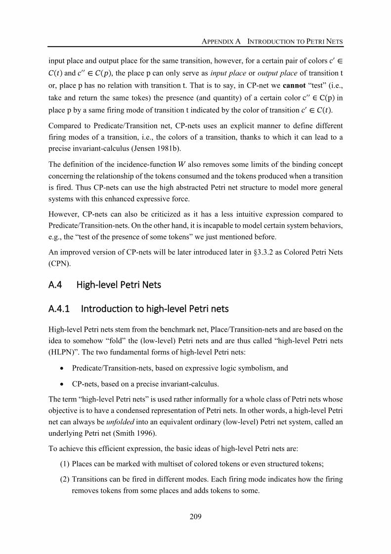
APPENDIX A INTRODUCTION TO PETRI NETS
209
input place and output place for the same transition, however, for a certain pair of colors 𝑐𝑐′ ∈𝐶𝐶(𝑡𝑡) and 𝑐𝑐′′ ∈ 𝐶𝐶(𝑇𝑇), the place p can only serve as input place or output place of transition t or, place p has no relation with transition t. That is to say, in CP-net we cannot “test” (i.e., take and return the same tokes) the presence (and quantity) of a certain color c′′ ∈ C(p) in place p by a same firing mode of transition t indicated by the color of transition 𝑐𝑐′ ∈ 𝐶𝐶(𝑡𝑡).
Compared to Predicate/Transition net, CP-nets uses an explicit manner to define different firing modes of a transition, i.e., the colors of a transition, thanks to which it can lead to a precise invariant-calculus (Jensen 1981b).
The definition of the incidence-function 𝑊𝑊 also removes some limits of the binding concept concerning the relationship of the tokens consumed and the tokens produced when a transition is fired. Thus CP-nets can use the high abstracted Petri net structure to model more general systems with this enhanced expressive force.
However, CP-nets can also be criticized as it has a less intuitive expression compared to Predicate/Transition-nets. On the other hand, it is incapable to model certain system behaviors, e.g., the “test of the presence of some tokens” we just mentioned before.
An improved version of CP-nets will be later introduced later in §3.3.2 as Colored Petri Nets (CPN).
A.4 High-level Petri Nets
A.4.1 Introduction to high-level Petri nets
High-level Petri nets stem from the benchmark net, Place/Transition-nets and are based on the idea to somehow “fold” the (low-level) Petri nets and are thus called “high-level Petri nets (HLPN)”. The two fundamental forms of high-level Petri nets:
• Predicate/Transition-nets, based on expressive logic symbolism, and
• CP-nets, based on a precise invariant-calculus.
The term “high-level Petri nets” is used rather informally for a whole class of Petri nets whose objective is to have a condensed representation of Petri nets. In other words, a high-level Petri net can always be unfolded into an equivalent ordinary (low-level) Petri net system, called an underlying Petri net (Smith 1996).
To achieve this efficient expression, the basic ideas of high-level Petri nets are:
(1) Places can be marked with multiset of colored tokens or even structured tokens;
(2) Transitions can be fired in different modes. Each firing mode indicates how the firing removes tokens from some places and adds tokens to some.

APPENDIX A INTRODUCTION TO PETRI NETS
210
Figure A-4 Efficient expression in high-level Petri nets
Figure A-4 shows how Petri nets with anonymous tokens are folded in high-level Petri nets by using colored tokens and structured tokens. In Figure A-4 (a), two railway routes are modeled in Petri nets and they can be either free or reserved. Figure A-4 (a) can be “folded” to Figure A-4 (b) by adding colors to different tokens and by assigning different firings to transition 𝑡𝑡3. For a more complex model, structured colored tokens can be used to further condense the model expression. As shown in Figure A-4 (d), tokens of 2-tuple can be used in place 𝑇𝑇9 to indicate that “a route 𝑉𝑉 is reserved by a train 𝑡𝑡𝑉𝑉”, which may require up to four places in (low level) Petri nets to express the same meaning.
A.4.2 High-level Petri Nets Standardization and PNML
High-level Petri nets are now standardized as the international standard ISO/IEC 15909 as a semi-graphical modeling language for the specification, design and analysis of discrete event systems (DES). Currently, this standard has two parts.
In Part 1 (ISO/IEC 2004), high-level Petri nets are conceptually and mathematically defined as a powerful method to provide unambiguous specifications and design descriptions of systems. It is recommended to be used for technical systems such as computer software and hardware, manufacturing, business processes, telecommunication networks, signaling, mechatronics, postal services, defense and avionics systems. It can also be used in biological and sociotechnical systems.
Part 2 (ISO/IEC 2011) defines the Petri Net Markup Language (PNML), an XML-based transfer format for Petri nets. It facilitates the exchange of Petri nets models among different Petri net tools and among different users. Besides the PNML Core Model, which is the common concept to all Petri nets, ISO/IEC 15909-2 also defines three concrete Petri net types:
t2
t3
(a) anonymous tokens (b) colored tokens
t1
p1: route(1) is free p2: route(1) is reserved
p4: route(2) is reservedp3: route(2) is free
p5: free p6: reserved
ROUTE ROUTE
𝑅𝑂𝑈𝑇𝐸 = 𝑟𝑜𝑢𝑡𝑒 1 , 𝑟𝑜𝑢𝑡𝑒(2 };
𝑟:𝑅𝑂𝑈𝑇𝐸;
𝑇𝑅𝐴𝐼𝑁 = 𝑡𝑟𝑎𝑖𝑛 1 , 𝑡𝑟𝑎𝑖𝑛(2 };
𝑡𝑟:𝑇𝑅𝐴𝐼𝑁.
t4
(c) structured tokens
ROUTE
TRAIN
p7: free routes
p8: trains
p9: routes reserved by trains
ROUTE x TRAIN
( , )
(d) definition

APPENDIX A INTRODUCTION TO PETRI NETS
211
• Place/Transition-Nets (P/T-Nets);
• High-level Petri Nets (HLPN);
• Symmetric Nets, which is inspired by well-formed nets.
This standard is a reference for developers of Petri net tools. It is also useful for researchers who will define new extensions and variants of Petri nets. It is worth noting that this standard just offers a definition framework that is still open for future extensions and variants of Petri nets to be added. The concrete and exact definition of Petri net variants and extensions (e.g., modularity constructs, hierarchies, time extensions), is not included in ISO/IEC 15909-2, but may be defined as Petri net type definition later in ISO/IEC 15909-3 (Kindler 2006).
There are some PNML implementations available for developers of Petri net software:
- PNML Framework (Hillah et al. 2010) is a free and open-source prototype implementation developed by LIP6 (French: Laboratoire d'Informatique de Paris 6) and LIPN (French: Laboratoire d'Informatique de Paris Nord);
- ePNK (Kindler 2012) is a graphical editor for Petri nets defined in PNML, which is developed by Technical University of Denmark using Graphical Modeling Framework (GMF) of Eclipse.
PNML is also supported by lots of Petri net tools, a list can be found in Table A-1.
A.5 Historical Development of CPN and Terminology
The Petri nets theory has an enormous vitality with new classes continuously being introduced and some definition of existing classes being renovated. A good example of the definition renovation can be found with colored Petri nets. However, this could also be very confusing in a terminological point of view.
It is thus very necessary to make clarify the development of colored Petri nets and to give some terminological remarks as some serious confusions about the colored Petri nets definitions could be found due to historical reasons.
We have introduced in §3.3.2 the CP-nets defined in (Jensen 1981a) as the first version of Colored* Petri nets. More precisely, we use CP81-nets for ease of comparison. The invention of CP81-nets was directly inspired by Predicate/Transition-nets defined in (Genrich and Lautenbach 1981), where the difference is that the relation between a firing mode and the involved colored tokens is defined explicitly by (arc) functions in CP81-nets, but is represented more implicitly by (arc) expressions in Pr/T-nets.
* In order to keep the consistency of American English spelling in this thesis, we always use “Colored” even though it was initially defined as “Coloured Petri Nets” in British English.

APPENDIX A INTRODUCTION TO PETRI NETS
212
However, for practical applications, it seems that the use of these functions (arc expressions) defined on transition colors in CP81-nets need always more time to build the model, and is more difficult to read and understand compared to Pr/T-nets. Moreover, with the development of symbolic invariant methods, there was a trend to define high-level nets mainly via syntactic inscriptions (Smith 1996). This situation finally gave birth to a mix of the two similar classes (i.e., CP81-nets and Pr/T-nets) in order to create a better Petri net class. This improved Petri net class was later introduced by Jensen under the name of “high-level Petri nets” or “HL-nets” in (Jensen 1982). Historically, it was not a good name as the researchers were used to referring the term “high-level” to a set of Petri net classes instead of a particular one.
As a compromise, Jensen reused the term “Colored Petri nets (CP-net)” in (Jensen 1986) to rename the aforementioned “HL-nets”, indicating that it was a subsequence of CP81-nets. Let us call the new version CP86-nets. Something new in this version of CP86-nets was that it has two forms of definition:
• CP-matrix*, a functional representation almost identical to CP81-nets;
• CP-graph, a graphical representation that uses the arc expression in the same ways as used by PrT-nets.
The two definitions are essentially identical, and a formal bi-directional translation is offered.
Since the 1990s, it seems that Jensen preferred the CP-graph representation of CP86-nets, probably because of its convenience for industrial applications. This representation was later cited as the definition of non-hierarchical CP-net in (Jensen 1991), CP-net in (Jensen 1998) and non-hierarchical Colored Petri Net in (Jensen and Kristensen 2009a). It is worth noting that the well-know CPN Tools also uses a modeling formalism similar to the CP-graph representation.
Meanwhile, the CP-matrix representation of CP86-nets (i.e., CP81-nets) is still active in academic or rather theoretical research as this form turns out to be more tractable when it comes to the analysis methods especially the invariant calculation. This choice would be very easy to understand when we consider the original motivation of Jensen to introduce CP81-nets (c.f. §A.3).
Due to the existence of different versions of colored Petri nets, it is very important to clearly indicate the particular definition used in a study, which is, unfortunately, often ignored by the researchers in their articles.
The situation is being even more confusing after the popularization of CPN Tools, which enhances the modeling power and the ease of use of colored Petri nets by offering the possibility of using some extensions that may only be supported by this tool. As CPN Tools is
* The name “CP-matrix” resulted from the incidence-function in its definition, which is traditionally called an incidence-matrix. See §A.3 for more details.

APPENDIX A INTRODUCTION TO PETRI NETS
213
also co-developed by Kurt Jensen, the inventor of colored Petri nets, in lots of papers (even some papers written by Jensen) the authors do not distinguish the colored Petri nets restricted to its formal definition, and those enhanced by the extensions offered in CPN Tools.
A.6 Petri Nets Software and Programming Languages
This subsection is mainly aimed to introduce the common software for the modeling and analysis of Petri nets.
Since CPN and WFN will be used in our modeling methods for a train control system (c.f. Chapter 4), the tools for these two formalisms are introduced in §3.3.2.4 and §3.3.3.4, respectively. §A.6.1 makes a brief introduction to some other Petri net software in literature and in practice. §A.6.2 shows that Petri nets have also promoted the development of a general-purpose programming language — Scala.
A.6.1 Petri Nets Software
We introduce and compare several widely used Petri net tools that keep updating. More Petri net tools can be found in (Störrle 1998) and on the Petri Net World* website.
Roméo (Gardey et al. 2005; Lime et al. 2009) is a Time Petri net designer and analyzer developed in IRCCyN (French: Institut de Recherche en Communications et Cybemétique de Nantes). It has a GUI to edit and design Time Petri nets and offers simulation and formal analysis. Roméo supports T-Time Petri nets (TPN) with a scheduling extension (stopwatches) and a parametric extension.
SNOOPY (Heiner et al. 2012) is a Petri net editor developed by Brandenburg University of Technology Cottbus-Senftenberg. SNOOPY supports a large set of Petri net and high-level Petri net classes with hierarchical, stochastic, time(d) extensions. It can be used together with S4 (Herajy and Heiner 2014), a steering and remote simulation server of SNOOPY, Charlie (Heiner et al. 2015), a Petri net model analyzer and Marcie (Heiner et al. 2013), a model checker for generalized stochastic Petri nets.
TimeNET (Zimmermann 2017) is a graphical modeling and analysis tool of colored Petri nets and Stochastic Petri nets developed by Technische Universität Ilmenau. It supports numerous performance evaluation based on Markov chains as well as some structural analysis algorithms and an interactive token-game simulation.
TINA (TIme Petri Net Analyzer) (Berthomieu et al. 2004) is an editing and analysis toolbox develop by LAAS-CNRS (Laboratory for Analysis and Architecture of Systems, French National Centre for Scientific Research). It supports models of Automata, Petri nets and Time Petri Nets with inhibitor arcs, read arcs, priorities, stopwatches, and a data handling extension * Available at http://www.informatik.uni-hamburg.de/TGI/PetriNets/.
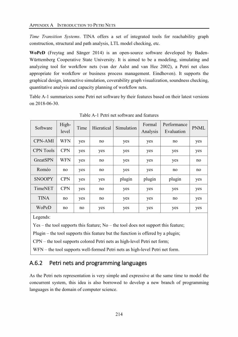
APPENDIX A INTRODUCTION TO PETRI NETS
214
Time Transition Systems. TINA offers a set of integrated tools for reachability graph construction, structural and path analysis, LTL model checking, etc.
WoPeD (Freytag and Sänger 2014) is an open-source software developed by Baden-Württemberg Cooperative State University. It is aimed to be a modeling, simulating and analyzing tool for workflow nets (van der Aalst and van Hee 2002), a Petri net class appropriate for workflow or business process management. Eindhoven). It supports the graphical design, interactive simulation, coverability graph visualization, soundness checking, quantitative analysis and capacity planning of workflow nets.
Table A-1 summarizes some Petri net software by their features based on their latest versions on 2018-06-30.
Table A-1 Petri net software and features
Software High-level
Time Hieratical Simulation Formal
Analysis Performance Evaluation
PNML
CPN-AMI WFN yes no yes yes no yes
CPN Tools CPN yes yes yes yes yes yes
GreatSPN WFN yes no yes yes yes no
Roméo no yes no yes yes no no
SNOOPY CPN yes yes plugin plugin plugin yes
TimeNET CPN yes no yes yes yes yes
TINA no yes no yes yes no yes
WoPeD no no yes yes yes yes yes
Legends:
Yes – the tool supports this feature; No – the tool does not support this feature;
Plugin – the tool supports this feature but the function is offered by a plugin;
CPN – the tool supports colored Petri nets as high-level Petri net form;
WFN – the tool supports well-formed Petri nets as high-level Petri net form.
A.6.2 Petri nets and programming languages
As the Petri nets representation is very simple and expressive at the same time to model the concurrent system, this idea is also borrowed to develop a new branch of programming languages in the domain of computer science.

APPENDIX A INTRODUCTION TO PETRI NETS
215
Functional Nets (Odersky 2000a) combine the ideas of functional programming and Petri nets. The fusion of the two powerful formalisms in different areas results in a programming style with simple notation and strong expressivity for general purpose.
Funnel (Odersky 2000b) was created as a programming language to implement Functional Nets. After that, a new programming language Scala was released following on from the work on Funnel.
Scala (Odersky and Rompf 2014) is a general-purpose and object-oriented programming language. Scala source code is compiled to Java bytecode to run on the Java platform (Java virtual machine) and is compatible with existing Java programs. Scala benefits from Petri nets to have a very concise design from its inception also has the support for functional programming. The good interoperability with Java and simply notation (compared to Java) makes it well-suited to a lot of development purposes.

216
Appendix B MODELING DETAILS OF ETCS ONBOARD SYSTEM B.1 ETCS Mode Transitions
B.1.1 Transitions Table in System Requirements Specification
The complete mode transitions table defined in section 4.6.2 in the specification (European Railway Agency 2016a) is shown in Table B-1.
Table B-1 Complete ETCS mode transitions
Table Source: “4.6.2 Transition Table” in (European Railway Agency 2016a)

APPENDIX B MODELING DETAILS OF ETCS ONBOARD SYSTEM
217
B.1.2 ETCS Mode Transitions Model
We have built a complete model for the mode transitions between the 12 considered modes: NP, SB, PS, SH, FS, SR, OS, NL, SF, IS, RV, PT. Other 5 modes (LS, SL, UN, TR, SN) are not yet included in this version.
The model uses the grouping views introduced in §4.4.2.3. The model for the mode transitions with target modes SB, FS, OS, SR and SH are separated in different groups according to their target modes, as shown in Figure 4-17 from (a) to (e). The mode transitions from any other modes to NP, NL, SF, IS, PS or RV are aggregated into the same group as shown in Figure 4-17 (f).
(a) From other modes to SB
(b) From other modes to FS

APPENDIX B MODELING DETAILS OF ETCS ONBOARD SYSTEM
218
(c) From other modes to OS
(d) From other modes to SR
(e) From other modes to SH
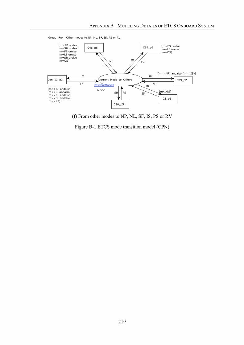
APPENDIX B MODELING DETAILS OF ETCS ONBOARD SYSTEM
219
(f) From other modes to NP, NL, SF, IS, PS or RV
Figure B-1 ETCS mode transition model (CPN)

APPENDIX B MODELING DETAILS OF ETCS ONBOARD SYSTEM
220
B.2 Procedure “Start of the Mission” (SoM)
B.2.1 Flowchart of Procedure “Start of the Mission” (SoM)
Figure B-2 Flowchart for Procedure “Start of the Mission” (SoM)
Source: Figure 5.4.4 in (European Railway Agency 2016a)

APPENDIX B MODELING DETAILS OF ETCS ONBOARD SYSTEM
221
B.3 Literal Model of Procedure “Start of the Mission” (SoM)
Figure B-3 shows the whole literal model in CPN Tools for procedure “Start of Mission” after the syntactic transformation from the flowchart Figure B-2.
Figure B-3 Literal CPN model of procedure “Start of Mission”
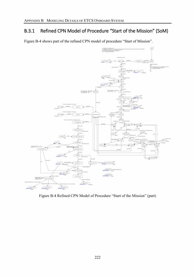
APPENDIX B MODELING DETAILS OF ETCS ONBOARD SYSTEM
222
B.3.1 Refined CPN Model of Procedure “Start of the Mission” (SoM)
Figure B-4 shows part of the refined CPN model of procedure “Start of Mission”.
Figure B-4 Refined CPN Model of Procedure “Start of the Mission” (part)

223
Appendix C IMPROVEMENT TO THE CASE STUDY IN §5.6 This appendix contains the improvements to a design defect found by verification in the case of §5.6. The original model is presented in (Xie et al. 2017a).
Figure C-1 shows the improved version of the train module (red part shows the modification). In the improved model, MA Request as a new message type sent from the train module to the RBC module. The MA request will be sent when:
• After the registration (1st MA request);
• Each time the train enters a new block;
• In case necessary (e.g., the situation in 2).
When the train received an MA with (EOA=POS), where POS is its current position, and it is not on the last block of the railway line, the train will again request for its MA.
Correspondingly, the RBC will no longer see the Position Report or Registration Request as MA Request, it will only send MA to the train after receiving an MA Request.

APPENDIX C IMPROVEMENT TO THE CASE STUDY IN §5.6
224
Figure C-1 Improved train module of the case study

225
REFERENCES van der Aalst WMP, van Hee KM. 2002. Workflow Management: Models, Methods, and Systems. Cambridge, MA, USA: MIT Press.
van der Aalst WMP, Stahl C, Westergaard M. 2013. Strategies for Modeling Complex Processes Using Colored Petri Nets. In: Jensen K, van der Aalst WMP, Balbo G, Koutny M, Wolf K, editors. Transactions on Petri Nets and Other Models of Concurrency VII. Berlin, Heidelberg: Springer Berlin Heidelberg. p. 6–55.
Abo R, Voisin L. 2013. Formal Implementation of Data Validation for Railway Safety-Related Systems with OVADO. In: Counsell S, Núñez M, editors. SEFM 2013: Software Engineering and Formal Methods. Madrid, Spain: Springer-Verlag New York, Inc. p. 221–236.
Abrial J-R. 2005. The B-book: Assigning Programs to Meanings. New York, NY, USA: Cambridge University Press.
Abrial J-R. 2010. Modeling in Event-B: System and Software Engineering. Cambridge: Cambridge University Press.
Aceituna D, Do H, Lee S-W. 2010. SQ^(2)E: An Approach to Requirements Validation with Scenario Question. In: 2010 Asia Pacific Software Engineering Conference. IEEE. p. 33–42.
Aceituna D, Do H, Lee S-W. 2011. Interactive requirements validation for reactive systems through virtual requirements prototype. In: 2011 Model-Driven Requirements Engineering Workshop. IEEE. p. 1–10.
Agha GA, De Cindio F, Rozenberg G, editors. 2001. Concurrent Object-Oriented Programming and Petri Nets. Berlin, Heidelberg: Springer Berlin Heidelberg (Lecture Notes in Computer Science).
Ahmad E, Dong Y, Larson B, Lü J, Tang T, Zhan N. 2015. Behavior modeling and verification of movement authority scenario of Chinese Train Control System using AADL. Sci China — Inf Sci. 58(11):1–20. doi:10.1007/s11432-015-5346-2.
Alur R, Brayton RK, Henzinger TA, Qadeer S, Rajamani SK. 1997. Partial-order reduction in symbolic state space exploration. In: Grumberg O, editor. CAV 1997: Computer Aided Verification. Berlin, Heidelberg: Springer Berlin Heidelberg. p. 340–351.
Alur R, Dill DL. 1994. A theory of timed automata. Theor Comput Sci. 126(2):183–235. doi:10.1016/0304-3975(94)90010-8.
Appel AW, MacQueen DB. 1991. Standard ML of New Jersey. p. 1–13.
Baarir S, Dutheillet C, Haddad S, Ilie JM. 2005. On the use of exact lumpability in partially symmetrical well-formed nets. In: Second International Conference on the Quantitative Evaluation of Systems (QEST’05). IEEE. p. 23–32.
Bahn D. 2017. DB presses ahead with train automation. [accessed 2017 Sep 1]. http://www.deutschebahn.com/en/Digitalization/automation.html.
Balbo G. 2001. Introduction to Stochastic Petri Nets. In: Brinksma E, Hermanns H, Katoen J-

REFERENCES
226
P, editors. Lectures on Formal Methods and Performance Analysis (EEF School 2000). Springer Berlin Heidelberg. p. 84–155.
Baranová Z, Barnat J, Kejstová K, Kučera T, Lauko H, Mrázek J, Ročkai P, Štill V. 2017. Model Checking of C and C++ with DIVINE 4. In: Automated Technology for Verification and Analysis (ATVA 2017). Vol. 10482. Springer. (LNCS). p. 201–207.
Barger P, Schön W, Bouali M. 2009. A Study of Railway ERTMS Safety with Colored Petri Nets. In: Bris GS, Martorell, editors. The European Safety and Reliability Conference (ESREL’09). Vol. 2. Prague, Czech Republic: Taylor & Francis Group. p. 1303–1309.
Batra M, Malik A, Dave M. 2013. Formal Methods : Benefits , Challenges and Future Direction. J Glob Res Comput Sci. 4(5):2–6.
Battiston E, De Cindio F, Mauri G. 1991. OBJSA Nets: A Class of High-level Nets Having Objects as Domains. In: Jensen K, Rozenberg G, editors. High-level Petri Nets. Berlin, Heidelberg: Springer Berlin Heidelberg. p. 189–212.
Bedők D. 2016. Application of Petri-nets in object-oriented environment. In: 2016 IEEE 17th International Symposium on Computational Intelligence and Informatics (CINTI 2016). IEEE. p. 117–122.
Behm P, Benoit P, Faivre A, Meynadier J-M. 1999. Météor: A Successful Application of B in a Large Project. In: Wing JM, Woodcock J, Davies J, editors. FM 1999: Formal Methods. Springer Berlin Heidelberg. p. 369–387.
Belloir N, Bruel J-M, Faudou R. 2014. Modélisation des exigences en UML/SysML. Rev Génie Logiciel.(111):6–12.
Bengtsson J, Larsen K, Larsson F, Pettersson P, Yi W. 1995. UPPAAL — a Tool Suite for Automatic Verification of Real-Time Systems. In: Hybrid Systems III: Verification and Control. Springer--Verlag. (Lecture Notes in Computer Science). p. 232–243.
Bérard B, Bidoit M, Finkel A, Laroussinie F, Petit A, Petrucci L, Schnoebelen P, McKenzie P. 2001. Systems and Software Verification: Model-Checking Techniques and Tools. Berlin, Heidelberg: Springer Berlin Heidelberg.
Bernardinello L, Cindio F. 1992. A survey of basic net models and modular net classes. In: Rozenberg G, editor. Advances in Petri Nets 1992. Berlin, Heidelberg: Springer Berlin Heidelberg. p. 304–351.
Berthelot G, Lri-Iie. 1986. Checking properties of nets using transformations. In: Rozenberg G, editor. Advances in Petri Nets 1985. Berlin, Heidelberg: Springer Berlin Heidelberg. p. 19–40.
Berthomieu B, Menasche M. 1983. An Enumerative Approach For Analyzing Time Petri Nets. In: the IFIP 9th World Computer Congress, volume 9 of Information Processing. North Holland/ IFIP. p. 41–46.
Berthomieu B, Ribet P-O, Vernadat F. 2004. The tool TINA – Construction of abstract state spaces for petri nets and time petri nets. Int J Prod Res. 42(14):2741–2756. doi:10.1080/00207540412331312688.
Bertot Y, Castéran P. 2004. Interactive Theorem Proving and Program Development — Coq’Art: The Calculus of Inductive Constructions. Berlin, Heidelberg: Springer Berlin
REFERENCES
227
Heidelberg (Texts in Theoretical Computer Science An EATCS Series).
Best E, Devillers R, Koutny M. 2001. Petri Net Algebra. Berlin, Heidelberg: Springer Berlin Heidelberg (Monographs in Theoretical Computer Science An EATCS Series).
Best E, Fernández C. 1986. Notations and terminology on Petri net theory. In: Arbeitspapiere der GMD No. 195. Gesellschaft für Mathematik und Datenverarbeitung, St. Augustin.
Bhuyan M, Ahasanol Kabir M. 2010. PLC based Automatic Railway Gate Control System. In: National Conference on Electronics and Telecommunications for Digital Bangladesh. Bangladesh Electronics Society, Dhaka, Bangladesh.
Bjørner D. 2003. New results and trends in formal techniques and tools for the development of software for transportation systems — A review. In: Tarnai G, Schnieder E, editors. FORMS2003: 4th Symposium on Formal Methods for Railway Operation and Control Systems. L’Harmattan Hongrie, Budapest, Hungary.
Bloem R, Cimatti A, Greimel K, Hofferek G, Könighofer R, Roveri M, Schuppan V, Seeber R. 2010. RATSY – A New Requirements Analysis Tool with Synthesis. In: Touili T, Cook B, Jackson P, editors. CAV 2010: 22nd International Conferenc on Computer Aided Verification. Vol. 217069. Edinburgh, UK: Springer-Verlag Berlin Heidelberg. p. 425–429.
Bošnački D, Leue S, Lluch Lafuente A. 2009. Partial-order reduction for general state exploring algorithms. Int J Softw Tools Technol Transf. 11(1):39–51. doi:10.1007/s10009-008-0093-y.
Bouajjani A, Tripakis S, Yovine S. 1997. On-the-fly symbolic model checking for real-time systems. In: Proceedings Real-Time Systems Symposium. IEEE Comput. Soc. p. 25–34.
Boukala MC, Petrucci L. 2011. Distributed Verification of Modular Systems. In: CompoNet and SUMo 2011.
Boulanger J-L. 2014. Formal Methods Applied to Industrial Complex Systems. Wiley (ISTE).
Bouyakoub S, Belkhir A. 2008. H-SMIL-Net: A Hierarchical Petri Net Model for SMIL Documents. In: Tenth International Conference on Computer Modeling and Simulation (uksim 2008). IEEE. p. 106–111.
Boyer B, Corre K, Legay A, Sedwards S. 2013. PLASMA-lab: A Flexible, Distributable Statistical Model Checking Library. In: Joshi K, Siegle M, Stoelinga M, D’Argenio PR, editors. QEST 2013: International Conference on Quantitative Evaluation of Systems. Berlin, Heidelberg: Springer Berlin Heidelberg. p. 160–164.
Brgan R, Poitrenaud D. 1995. An efficient algorithm for the computation of stubborn sets of well formed Petri Nets. In: De Michelis G, Diaz M, editors. ICATPN 1995: Application and Theory of Petri Nets 1995. Berlin, Heidelberg: Springer Berlin Heidelberg. p. 121–140.
Bu L, Wang Q, Chen X, Wang L, Zhang T, Zhao J, Li X. 2011. Toward online hybrid systems model checking of cyber-physical systems’ time-bounded short-run behavior. ACM SIGBED Rev. 8(2):7–10. doi:10.1145/2000367.2000368.
Buchholz P. 1994. Hierarchical High Level Petri Nets for complex system analysis. In: Valette R, editor. Application and Theory of Petri Nets 1994Application and Theory of Petri Nets (ICATPN) 1994. Zaragoza, Spain: Springer Berlin Heidelberg. p. 119–138.
Burch JR, Clarke EM, McMillan KL, Dill DL, Hwang LJ. 1992. Symbolic model checking: 10^20

REFERENCES
228
States and beyond. Inf Comput. 98(2):142–170. doi:10.1016/0890-5401(92)90017-A.
Camurri A, Franchi P, Gandolfo F. 1991. A timed colored Petri nets approach to process scheduling. In: [1991] Proceedings, Advanced Computer Technology, Reliable Systems and Applications. p. 304–309.
Cassandras CG, Lafortune S. 2009. Introduction to Discrete Event Systems (Second Edition). Springer US (SpringerLink Engineering).
CENELEC. 2003. EN 50129:2003—Railway applications. Communication, signalling and processing systems. Safety related electronic systems for signalling.
CENELEC. 2010. EN 50159:2010—Railway applications. Communication, signalling and processing systems. Safety-related communication in transmission systems.
CENELEC. 2011. EN 50128:2011—Railway applications - Communication, signalling and processing systems - Software for railway control and protection systems.
CENELEC. 2017. EN 50126-1:2017—Railway Applications. The Specification and Demonstration of Reliability, Availability, Maintainability and Safety (RAMS). Generic RAMS Process.
Cheng A, Christensen S, Mortensen KH. 1996. Model Checking Coloured Petri Nets Exploiting Strongly Connected Components. In: International Workshop on Discrete Event Systems (WODES’96). Vol. 26. Edinburgh, Scotland, UK.
Chiappini A, Cimatti A, Macchi L, Rebollo O, Roveri M, Susi A, Tonetta S, Vittorini B. 2010. Formalization and validation of a subset of the European Train Control System. In: ICSE2010: 32nd ACM/IEEE International Conference on Software Engineering. Vol. 2. ACM Press. p. 109–118.
Chiola G, Dutheillet C, Franceschinis G, Haddad S. 1991a. On Well-Formed Coloured Nets and Their Symbolic Reachability Graph. In: High-level Petri Nets. Berlin, Heidelberg: Springer Berlin Heidelberg. p. 373–396.
Chiola G, Dutheillet C, Franceschinis G, Haddad S. 1991b. Stochastic Well-Formed Coloured Nets and Multiprocessor Modelling Applications. In: Jensen K, Rozenberg G, editors. High-level Petri Nets. Berlin, Heidelberg: Springer Berlin Heidelberg. p. 504–530.
Chiola G, Dutheillet C, Franceschinis G, Haddad S. 1993. Stochastic well-formed colored nets and symmetric modeling applications. IEEE Trans Comput. 42(11):1343–1360. doi:10.1109/12.247838.
Chiola G, Dutheillet C, Franceschinis G, Haddad S. 1997. A symbolic reachability graph for coloured petri nets. Theor Comput Sci. 176(1–2):39–65. doi:10.1016/S0304-3975(96)00010-2.
Chiola G, Franceschinis G, Gaeta R. 1992. A symbolic simulation mechanism for well-formed coloured Petri nets. In: Proceedings. 25th Annual Simulation Symposium. IEEE Comput. Soc. Press. p. 192–201.
Chiola G, Franceschinis G, Gaeta R, Ribaudo M. 1995. GreatSPN 1.7: Graphical editor and analyzer for timed and stochastic Petri nets. Perform Eval. 24(1–2):47–68. doi:10.1016/0166-5316(95)00008-L.

REFERENCES
229
Cho CH, Choi DH, Quan ZH, Choi SA, Park GS, Ryou MS. 2011. Modeling of CBTC carborne ATO functions using SCADE. In: 2011 11th International Conference on Control, Automation and Systems. p. 1089–1093.
Choi J-K, Cho H, Oh H-S, Kim K-H, Bhang M-J, Yu I-S, Ryu H-G. 2015. Challenges of LTE high-speed railway network to coexist with LTE public safety network. In: 17th International Conference on Advanced Communication Technology (ICACT 2015). p. 543–547.
Choppy C, Petrucci L. 2004. Towards a methodology for modeling with Petri nets. Proc Work Pract Use Coloured Petri Nets Aarhus Denmark.(October):39–56.
Choppy C, Reggio G. 2006. A formally grounded software specification method. J Log Algebr Program. 67(1–2):52–86. doi:10.1016/j.jlap.2005.09.003.
Christensen S, Damgaard Hansen N. 1994. Coloured Petri Nets extended with channels for synchronous communication. In: Valette R, editor. ICATPN 1994: Application and Theory of Petri Nets 1994. Berlin, Heidelberg: Springer Berlin Heidelberg. p. 159–178.
Christensen S, Kristensen LM, Mailund T. 2001. A Sweep-Line Method for State Space Exploration. In: Margaria T, Yi W, editors. TACAS 2001: Tools and Algorithms for the Construction and Analysis of Systems. p. 450–464.
Christensen S, Mortensen KH. 1996. Design/CPN ASK-CTL Manual (Version 0.9).
Christensen S, Petrucci L. 1992. Towards a modular analysis of coloured Petri nets. Appl Theory Petri Nets 1992.:113–133.
Christensen S, Petrucci L. 1995. Modular State Space Analysis of Coloured Petri Nets. In: Application and Theory of Petri Nets 1995. Turin, Italy.
Christensen S, Petrucci L. 2000. Modular Analysis of Petri Nets. Comput J. 43(3):224–242. doi:10.1093/comjnl/43.3.224.
Clarke EM, Emerson EA. 1981. Design and synthesis of synchronization skeletons using branching time temporal logic. In: Kozen D, editor. Logics of Programs. Berlin/Heidelberg: Springer-Verlag. p. 52–71.
Clarke EM, Grumberg O, Minea M, Peled D. 1999. State space reduction using partial order techniques. Int J Softw Tools Technol Transf. 2(3):279–287. doi:10.1007/s100090050035.
Clarke EM, Long DE, McMillan KL. 1989. Compositional model checking. In: Parikh R, editor. Proceedings of the 4th Annual Symposium on Logic in computer science. IEEE Computer Society Press. p. 353–362.
Di Claudio M, Fantechi A, Martelli G, Menabeni S, Nesi P. 2014. Model-based development of an automatic train operation component for communication based train control. In: 17th International IEEE Conference on Intelligent Transportation Systems (ITSC). IEEE. p. 1015–1020.
Colange M, Baarir S, Kordon F, Thierry-Mieg Y. 2011. Crocodile: A Symbolic/Symbolic Tool for the Analysis of Symmetric Nets with Bag. In: Kristensen LM, Petrucci L, editors. PETRI NETS 2011: Applications and Theory of Petri Nets. Berlin, Heidelberg: Springer Berlin Heidelberg. p. 338–347.
Courant J, Monin J-F. 2006. Defending the Bank with a Proof Assistant. In: 6th International

REFERENCES
230
Workshop on Issues inthe Theory of Security (WITS 2006). p. 87–98.
Couvreur JM, Martínez J. 1991. Linear invariants in commutative high level nets. In: Rozenberg G, editor. Advances in Petri Nets 1990. Springer Berlin Heidelberg. p. 146–164.
Dandanell B, Gørtz J, Pedersen JS, Zierau E. 1993. Experiences from applications of RAISE. In: Woodcock JCP, Larsen PG, editors. FME ’93: Industrial-Strength Formal Methods. Berlin/Heidelberg: Springer-Verlag. p. 52–63.
Deng Y, Grumbach S, Monin J-F. 2011. A Framework for Verifying Data-Centric Protocols. In: Bruni R, Dingel J, editors. FMOODS 2011, FORTE 2011: Formal Techniques for Distributed Systems. Berlin, Heidelberg: Springer Berlin Heidelberg. p. 106–120.
Deng Y, Monin J-F. 2009. Verifying Self-stabilizing Population Protocols with Coq. In: 2009 Third IEEE International Symposium on Theoretical Aspects of Software Engineering. IEEE. p. 201–208.
Dias da Silva L, Perkusich A. 2003. Formal Verification of Component-Based Software Systems. In: New Technologies for Information Systems, Proceedings of the 3rd International Workshop on New Developments in Digital Libraries, NDDL 2003, and the 1st International Workshop on Validation and Verification of Software for Enterprise Information Systems, . ICEIS press. p. 113–124.
Dwyer MB, Avrunin GS, Corbett JC. 1999. Patterns in property specifications for finite-state verification. In: ICSE‘99: the 21st international conference on Software engineering. New York, New York, USA: ACM Press. p. 411–420.
EEIG ERTMS Users Group. 2016. Mission of the ERTMS Users Group.
Emerson EA, Halpern JY. 1986. “Sometimes” and “not never” revisited: on branching versus linear time temporal logic. J ACM. 33(1):151–178. doi:10.1145/4904.4999.
Emerson EA, Jha S, Peled D. 1997. Combining partial order and symmetry reductions. In: Brinksma E, editor. TACAS 1997: Tools and Algorithms for the Construction and Analysis of Systems. Berlin, Heidelberg: Springer Berlin Heidelberg. p. 19–34.
Emerson EA, Sistla AP. 1996. Symmetry and model checking. Form Methods Syst Des. 9(1–2):105–131. doi:10.1007/BF00625970.
Emerson EA, Trefler RJ. 1999. From Asymmetry to Full Symmetry: New Techniques for Symmetry Reduction in Model Checking. In: Pierre L, Kropf T, editors. CHARME 1999: Correct Hardware Design and Verification Methods. Berlin, Heidelberg: Springer Berlin Heidelberg. p. 142–157.
Emery D (TRANSP-O. 2017. Towards Automatic Train Operation for long distance services: State-of-the art and challenges. In: 17th Swiss Transport Research Conference (STRC 2017). Ascona, TI, CH.
Eshuis R, Dehnert J. 2003. Reactive Petri Nets for Workflow Modeling. Appl Theory Petri Nets 2003. 2679:295–314. doi:10.1007/3-540-44919-1_20.
Esparza J, Hoffmann P. 2016. Reduction Rules for Colored Workflow Nets. In: Fundamental Approaches to Software Engineering: 19th International Conference (FASE 2016). p. 342–358.

REFERENCES
231
Espensen KL, Kjeldsen MK, Kristensen LM, Westergaard M. 2009. Towards Automatic Code-generation from Process-partitioned Coloured Petri Nets.
European Commission. 2008. Directive 2008/57/EC of the European Parliament and of the Council of 17 June 2008 on the interoperability of the rail system within the Community.
European Commission. 2014. 2014/897/EU: Commission Recommendation of 5 December 2014 on matters related to the placing in service and use of structural subsystems and vehicles under Directives 2008/57/EC and 2004/49/EC of the European Parliament and of the Council.
European Commission. 2016. Commission Regulation (EU) 2016/919 of 27 May 2016 on the technical specification for interoperability relating to the ‘control-command and signalling’ subsystems of the rail system in the European Union (TSI CCS).
European Commission. 2017a. Fact Sheets on ERTMS. [accessed 2017 Jan 5]. https://ec.europa.eu/transport/sites/transport/files/2017-01-05-memo-ertms.pdf.
European Commission. 2017b. Commission Implementing Regulation (EU) 2017/6 of 5 January 2017 on the European Rail Traffic Management System European deployment plan.
European Railway Agency. 2016a. ERTMS/ETCS System Requirements Specification (SUBSET-026) v3.6.0.
European Railway Agency. 2016b. ERTMS/ETCS Test Cases Related to Features (SUBSET-076-5-2) v3.1.0.
European Railway Agency. 2016c. ERTMS/ETCS Test Sequences (SUBSET-076-6-3) v3.0.0.
European Railway Agency. 2016d. ERTMS UNIT Scope of the Test Specifications (SUBSET-076-7) v3.1.0.
European Union Agency for Railways. 2016. TSI CCS Current Legal Reference. [accessed 2018 Apr 30]. http://www.era.europa.eu/Core-Activities/ERTMS/Pages/Current-Legal-Reference.aspx.
European Union Agency for Railways. 2017. ETCS TEST PLAN AND METHODOLOGY FOR SS-076 (v1.0.0).
Evangelista S, Haddad S, Pradat-Peyre J-F. 2005. Syntactical Colored Petri Nets Reductions. In: Peled DA, Tsay Y-K, editors. Automated Technology for Verification and Analysis: Third International Symposium, ATVA 2005, Taipei, Taiwan, October 4-7, 2005. Proceedings. Berlin, Heidelberg: Springer Berlin Heidelberg. p. 202–216.
Faber J, Jacobs S, Sofronie-Stokkermans V. 2007. Verifying CSP-OZ-DC Specifications with Complex Data Types and Timing Parameters. In: IFM’07: Proceedings of the 6th International Conference on Integrated Formal Methods. Berlin, Heidelberg: Springer-Verlag. p. 233–252.
Fantechi A, Fokkink W, Morzenti A. 2012. Some Trends in Formal Methods Applications to Railway Signaling. In: Gnesi S, Margaria T, editors. Formal Methods for Industrial Critical Systems: A Survey of Applications. Hoboken, NJ, USA: John Wiley & Sons, Inc. p. 61–84.
Fasie MV. 2013. An Eclipse based Development Environment for RAISE. Technical University of Denmark.
Ferrari A, Spagnolo GO, Martelli G, Menabeni S. 2012. Product Line Engineering Applied to

REFERENCES
232
CBTC Systems Development. In: Margaria T, Steffen B, editors. Leveraging Applications of Formal Methods, Verification and Validation. Applications and Case Studies (ISoLA 2012). Heraklion, Crete, Greece. p. 216–230.
Fidge C. 1994. A Comparative Introduction to CSP, CCS and LOTOS.
Freytag T, Sänger M. 2014. WoPeD - An educational tool for workflow nets. In: Proceedings of the BPM Demo Sessions. Vol. 1295. Eindhoven, The Netherlands. p. 31–35.
Fronc Ł, Duret-Lutz A. 2013. LTL Model Checking with Neco. In: Proceedings of the 11th International Symposium on Automated Technology for Verification and Analysis (ATVA’13). Vol. 8172. Hanoi, Vietnam: Springer. (Lecture Notes in Computer Science). p. 451–454.
Gardey G, Lime D, Magnin M, Roux OH. 2005. Romeo: A Tool for Analyzing Time Petri Nets. In: Computer Aided Verification. Vol. 1. Springer. p. 418–423.
Genrich HJ. 1986. Predicate/Transition Nets. In: Brauer W, Reisig W, Rozenberg G, editors. Petri Nets: Central Models and Their Properties (ACPN 1986). Berlin/Heidelberg: Springer Berlin Heidelberg. p. 207–247.
Genrich HJ, Lautenbach K. 1979. The analysis of distributed systems by means of predicate/transition-nets. In: Kahn G, editor. Semantics of Concurrent Computation. Berlin/Heidelberg: Springer. p. 123–146.
Genrich HJ, Lautenbach K. 1981. System modelling with high-level Petri nets. Theor Comput Sci. 13(1):109–135. doi:10.1016/0304-3975(81)90113-4.
Gonçalves M, Fernandes JM. 2013. Guidelines for Modelling Reactive Systems with Coloured Petri Nets. In: Machado RJ, Maciel RSP, Rubin J, Botterweck G, editors. MOMPES 2012: Model-Based Methodologies for Pervasive and Embedded Software. Berlin, Heidelberg: Springer Berlin Heidelberg. p. 126–137.
Graf S, Steffen B. 1990. Compositional minimization of finite state systems. In: Clarke EM, Kurshan RP, editors. Computer-Aided Verification. Berlin/Heidelberg: Springer-Verlag. p. 186–196.
Graf S, Steffen B, Lüttgen G. 1996. Compositional minimisation of finite state systems using interface specifications. Form Asp Comput. 8(5):607–616. doi:10.1007/BF01211911.
Grumberg O, Long DE. 1991. Model checking and modular verification. In: Baeten JCM, Groote JF, editors. CONCUR 1991: International Conference on Concurrency Theory. Berlin, Heidelberg: Springer Berlin Heidelberg. p. 250–265.
Gu F, Zhang X, Chen M, Große D, Drechsler R. 2016. Quantitative timing analysis of UML activity diagrams using statistical model checking. In: 2016 Design, Automation & Test in Europe Conference & Exhibition (DATE). p. 780–785.
Guan S-U, Yu H-Y, Yang J-S. 1998. A prioritized Petri net model and its application in distributed multimedia systems. IEEE Trans Comput. 47(4):477–481. doi:10.1109/12.675716.
Haddad S. 1987. Une catégorie régulière de réseau de Petri de haut-niveau : définition, propriétés et réductions. Application à la validation de systèmes distribués. Universite P. et M. Curie, Paris, France.
Haddad S. 1991. A Reduction Theory for Coloured Nets. In: Jensen K, Rozenberg G, editors.
REFERENCES
233
High-level Petri Nets: Theory and Application. Berlin, Heidelberg: Springer Berlin Heidelberg. p. 399–425.
Haddad S, Ilié JM, Taghelit M, Zouari B. 1995. Symbolic reachability graph and partial symmetries. In: De Michelis G, Diaz M, editors. ICATPN 1995: International Conference on Application and Theory of Petri Nets 1995. Berlin, Heidelberg: Springer Berlin Heidelberg. p. 238–257.
Haddad S, Kordon F, Petrucci L, Pradat-Peyre J-F, Treves L. 2009. Efficient state-based analysis by introducing bags in Petri nets color domains. In: 2009 American Control Conference. IEEE. p. 5018–5025.
Haddad S, Pradat-Peyre J-F. 2004. Efficient Reductions for LTL Formulae Verification. Paris, France.
Hadjidj R, Boucheneb H. 2006. On-the-fly TCTL model checking for Time Petri Nets using state class graphs. In: Sixth International Conference on Application of Concurrency to System Design (ACSD’06). IEEE. p. 111–122.
Hansen KM. 1994. Formalising Railway Interlocking Systems. In: Nordic Seminar on Dependable Computing Systems 1994. Technical University of Denmark, DK 2800 Lyngby, Denmark. p. 83–94.
Haxthausen AE, Pedersen JS, Prehn S. 1993. Raise: a product supporting industrial use of formal methods. Tech Sci Informatiques. 12(3):319–346.
Haxthausen AE, Peleska J. 2000. Formal development and verification of a distributed railway control system. IEEE Trans Softw Eng. 26(8):687–701. doi:10.1109/32.879808.
He X, Murata T. 2005. High-Level Petri Nets—Extensions, Analysis, and Applications. In: The Electrical Engineering Handbook. Elsevier. p. 459–475.
Heddebaut M. 2009. Leaky Waveguide for Train-to-Wayside Communication-Based Train Control. IEEE Trans Veh Technol. 58(3):1068–1076. doi:10.1109/TVT.2008.928635.
Heiner M, Herajy M, Liu F, Rohr C, Schwarick M. 2012. Snoopy – A Unifying Petri Net Tool. In: Proc. PETRI NETS 2012. Vol. 7347. Springer. (LNCS). p. 398–407.
Heiner M, Rohr C, Schwarick M. 2013. MARCIE – Model Checking and Reachability Analysis Done Efficiently. In: Colom J-M, Desel J, editors. PETRI NETS 2013: Application and Theory of Petri Nets and Concurrency. Berlin, Heidelberg: Springer Berlin Heidelberg. p. 389–399.
Heiner M, Schwarick M, Wegener J-T. 2015. Charlie – An Extensible Petri Net Analysis Tool. In: Devillers R, Valmari A, editors. Proc. PETRI NETS 2015. Vol. 9115. Springer. (LNCS). p. 200–211.
Henzinger TA. 2000. The Theory of Hybrid Automata. In: Inan MK, Kurshan RP, editors. Verification of Digital and Hybrid Systems. Berlin, Heidelberg: Springer Berlin Heidelberg. p. 265–292.
Herajy M, Heiner M. 2014. A Steering Server for Collaborative Simulation of Quantitative Petri Nets. In: Ciardo G, Kindler E, editors. PETRI NETS 2014: Application and Theory of Petri Nets and Concurrency. Cham: Springer International Publishing. p. 374–384.
Hillah LM, Kordon F, Petrucci L, Trèves N. 2010. PNML Framework: An Extendable Reference

REFERENCES
234
Implementation of the Petri Net Markup Language. In: Lilius J, Penczek W, editors. Berlin, Heidelberg: Springer Berlin Heidelberg. p. 318–327.
Hoare CAR. 1978. Communicating sequential processes. Commun ACM. 21(8):666–677. doi:10.1145/359576.359585.
Hongli Zhao, Tianhua Xu, Tao Tang. 2009. Towards modeling and evaluation of availability of communication based train control (CBTC) system. In: 2009 IEEE International Conference on Communications Technology and Applications. IEEE. p. 860–863.
Hu G. 2008. A Formal Specification of UML Class and State Diagrams. In: Lee R, editor. Software Engineering, Artificial Intelligence, Networking and Parallel/Distributed Computing. Berlin, Heidelberg: Springer Berlin Heidelberg. p. 247–257.
Huber P, Jensen AM, Jepsen LO, Jensen K. 1986. Reachability trees for high-level petri nets. Theor Comput Sci. 45:261–292. doi:10.1016/0304-3975(86)90046-0.
Huber P, Jensen K, Shapiro RM. 1991. Hierarchies in coloured petri nets. In: Rozenberg G, editor. Berlin, Heidelberg: Springer Berlin Heidelberg. p. 313–341.
IEC. 2003. IEC 61131-3 Programmable Controllers – Part 3: Programming languages.
IEC. 2009. IEC 62267:2009—Railway applications - Automated Urban Guided Transport (AUGT) - Safety Requirements.
IEC. 2014. IEC 62290:2014—Railway applications - Urban guided transport management and command/control systems.
IEEE. 1993. IEEE Std 1164-1993 - IEEE Standard Multivalue Logic System for VHDL Model Interoperability (Std_logic_1164). doi:10.1109/IEEESTD.1993.115571.
IEEE. 2006. IEEE Std. 1364-2005 - IEEE Standard for Verilog Hardware Description Language. doi:10.1109/IEEESTD.2006.99495.
IEEE. 2012. IEEE Std. 1666-2011 - IEEE Standard for Standard SystemC Language Reference Manual. doi:10.1109/IEEESTD.2012.6134619.
IEEE. 2017. IEEE Std. 1800-2017 - IEEE Standard for SystemVerilog—Unified Hardware Design, Specification, and Verification Language. doi:10.1109/IEEESTD.2018.8299595.
IEEE Std. 2004. IEEE Standard for Communications-Based Train Control (CBTC) Performance and Functional Requirements. IEEE Std 14741-2004 (Revision IEEE Std 14741-1999).:0_1-45. doi:10.1109/IEEESTD.2004.95746.
Ilié JM, Ajami K. 1997. Model checking through symbolic reachability graph. In: Bidoit M, Dauchet M, editors. TAPSOFT ’97: Theory and Practice of Software Development. Berlin, Heidelberg: Springer Berlin Heidelberg. p. 213–224.
ISO/IEC. 2004. ISO/IEC 15909-1:2004 - Systems and software engineering - High-level Petri nets - Part 1: Concepts, definitions and graphical notation. :38.
ISO/IEC. 2005. ISO/IEC 19501:2005 (OMG-UML VER 1.3) — Information technology - Open Distributed Processing - Unified Modeling Language (UML) Version 1.4.2.
ISO/IEC. 2011. ISO/IEC 15909-2:2011 - Systems and software engineering - High-level Petri nets - Part 2: Transfer format. :102.

REFERENCES
235
ISO. 1989. ISO 8807:1989 — Information processing systems - Open Systems Interconnection - LOTOS - A formal description technique based on the temporal ordering of observational behaviour.
Issad M, Kloul L, Rauzy A. 2014. A Model-Based Methodology to Formalize Specifications of Railway Systems. In: Ortmeier F, Rauzy A, editors. IMBSA 2014: 4th International Symposium of Model-Based Safety and Assessment. Munich, Germany. p. 28–42.
Issad M, Koul L, Rauzy A. 2015. A contribution to safety analysis of railway CBTC systems using Scola. In: ESREL 2015: Safety and Reliability of Complex Engineered Systems. Zurich, Switzerland: CRC Press. p. 459–467.
ITU-T. 2016. Recommendation Z.100 (04/16) : Specification and Description Language (SDL).
Jabri S, El Koursi EM, Lemaire E, Bourdeaud’huy T. 2009. Modelling of the European Rail Traffic Management System (ERTMS) for checking objectives. IFAC Proc Vol. 42(15):84–90. doi:10.3182/20090902-3-US-2007.0097.
Janczura CW. 1999. Modelling and Analysis of Railway Network Control Logic using Coloured Petri Nets. University of South Australia.
Jansen L, Meyer zu Hörste M, Schnieder E. 1998. Technical Issues in Modelling the European Train Control System (ETCS) Using Coloured Petri Nets and the Design/CPN Tools. In: Jensen K, editor. Workshop on Practical Use of Coloured Petri Nets and Design. Daimi PB-532, Aarhus, Denmark: Aarhus University. p. 103–115.
Jensen K. 1981a. Coloured Petri Nets and the Invariant-Method. Theor Comput Sci. 14(3):317–336. doi:10.1016/0304-3975(81)90049-9.
Jensen K. 1981b. How to find invariants for coloured Petri nets. In: Gruska J, Chytil M, editors. Mathematical Foundations of Computer Science 1981: Proceedings, 10th Symposium {Š}trbsk{é} Pleso, Czechoslovakia August 31 -- September 4, 1981. Berlin, Heidelberg: Springer Berlin Heidelberg. p. 327–338.
Jensen K. 1982. High-Level Petri Nets. In: Pagnoni A, Rozenberg G, editors. 3rd European Workshop on Application and Theory of Petri Nets. Varenna, Italy: Springer Berlin Heidelberg. p. 166–180.
Jensen K. 1986. Coloured Petri Nets. In: Brauer W, Reisig W, Rozenberg G, editors. Petri Nets: Central Models and Their Properties (ACPN 1986). Springer Berlin Heidelberg. p. 248–299.
Jensen K. 1991. Coloured petri nets: A high level language for system design and analysis. In: Rozenberg G, editor. Advances in Petri Nets 1990 (Lecture Notes in Computer Science). Vol. 483. Springer Berlin Heidelberg. p. 342–416.
Jensen K. 1992. Hierarchical Coloured Petri Nets. In: Jensen K, editor. Coloured Petri Nets (EATCS Monographs in Theoretical Computer Science). Berlin, Heidelberg: Springer Berlin Heidelberg. p. 89–121.
Jensen K. 1997. Coloured Petri Nets: Basic Concepts, Analysis Methods and Practical Use. Volume 3. Berlin, Heidelberg: Springer Berlin Heidelberg (Monographs in Theoretical Computer Science An EATCS Series).
Jensen K. 1998. An introduction to the practical use of coloured Petri Nets. In: Reisig W, Rozenberg G, editors. ACPN 1996: Lectures on Petri Nets II: Applications. p. 237–292.

REFERENCES
236
Jensen K, Kristensen LM. 2009a. Formal Definition of Non-hierarchical Coloured Petri Nets. In: Jensen K, Kristensen Lars M., editors. Coloured Petri Nets (Modelling and Validation of Concurrent Systems). Berlin, Heidelberg: Springer Berlin Heidelberg. p. 79–94.
Jensen K, Kristensen LM. 2009b. CPN ML Programming. In: Jensen K, Kristensen Lars M., editors. Coloured Petri Nets (Modelling and Validation of Concurrent Systems). Berlin, Heidelberg: Springer Berlin Heidelberg. p. 43–77.
Jensen K, Kristensen LM, Wells L. 2007. Coloured Petri Nets and CPN Tools for modelling and validation of concurrent systems. Int J Softw Tools Technol Transf. 9(3–4):213–254. doi:10.1007/s10009-007-0038-x.
Joel F, Wu H, Hyung L-K. 1988. Reduction Method Of Coloured Petri Nets. IEEE Int Conf Syst Man, Cybern. 2:984–987. doi:10.1109/ICSMC.1988.712855.
John K-H, Tiegelkamp M. 2001. IEC 61131-3: Programming Industrial Automation Systems. Berlin, Heidelberg: Springer Berlin Heidelberg.
Josserand P, Forman HW. 1957. Rights of trains (5th edition). 5th editio. New York: Simmons-Boardman Pub. Corp.
Junttila T. 2003. On the symmetry reduction method for Petri nets and similar formalisms. Helsinki University of Technology.
Kapur D, Winter VL, Berg RS. 2001. Designing a Controller for a Multi-Train Multi-Track System. Electron Notes Theor Comput Sci. 50(1):65–79. doi:10.1016/S1571-0661(04)00166-5.
Khan U, Ahmad J, Saeed T, Mirza SH. 2016. On the real time modeling of interlocking system of passenger lines of Rawalpindi Cantt train station. Complex Adapt Syst Model. 4(1):17. doi:10.1186/s40294-016-0028-5.
Kichenside GM, Williams A. 1998. Two Centuries of Railway Signalling. Oxford Publishing.
Kindler E. 2006. The petri net markup language and iso/iec 15909-2: Concepts, status, and future directions. Entwurf komplexer Autom. 9(May):35–55.
Kindler E. 2012. The ePNK: A generic PNML tool - Users’ and Developers’ Guide for Version 1.0.0. Kongens Lyngby, Denmark.
Kissell TE. 2002. Industrial Electronics: Applications for Programmable Controllers, Instrumentation and Process Control, and Electrical Machines and Motor Controls (3rd Edition). 3rd ed. Prentice Hall.
Klai K. 2003. Réseaux de Petri : Vérification Modulaire et Symbolique. Paris 6.
Kordon F, Paviot-Adet E. 1999. Using CPN-AMI to Validate a Safe Channel Protocol. In: Proceedings of the International Conference on Theory and Applications of Petri Nets - Tool presentation part. Williamsburg, USA.
Kristensen LM, Petrucci L. 2004. An Approach to Distributed State Space Exploration for Coloured Petri Nets. In: Cortadella J, Reisig W, editors. ICATPN 2004: Applications and Theory of Petri Nets 2004. Berlin, Heidelberg: Springer Berlin Heidelberg. p. 474–483.
Kristensen LM, Westergaard M. 2010. Automatic Structure-Based Code Generation from Coloured Petri Nets: A Proof of Concept. In: Kowalewski S, Roveri M, editors. FMICS 2010:
REFERENCES
237
Formal Methods for Industrial Critical Systems. Berlin, Heidelberg: Springer Berlin Heidelberg. p. 215–230.
Kuehlmann A, Eijk CAJ. 2002. Combinational and Sequential Equivalence Checking. In: Hassoun S, Sasao T, editors. Logic Synthesis and Verification. Boston, MA: Springer US. p. 343–372.
Kwiatkowska M, Norman G, Parker D. 2002. PRISM: Probabilistic Symbolic Model Checker. In: Field T, Harrison PG, Bradley J, Harder U, editors. TOOLS 2002: International Conference on Modelling Techniques and Tools for Computer Performance Evaluation. Berlin, Heidelberg: Springer Berlin Heidelberg. p. 200–204.
Lakos C, Petrucci L. 2004. Modular analysis of systems composed of semiautonomous subsystems. Appl Concurr to Syst Des 2004 ACSD 2004 Proceedings Fourth Int Conf.:185–194. doi:10.1109/CSD.2004.1309131.
Lakos C, Petrucci L. 2007a. Modular state space exploration for timed petri nets. Int J Softw Tools Technol Transf. 9(3–4):393–411. doi:10.1007/s10009-007-0033-2.
Lakos C, Petrucci L. 2007b. Modular State Spaces and Place Fusion. In: International Workshop on Petri Nets and Software Engineering (PNSE’07, associated with Petri Nets’07). p. 175–190.
Latvala T, Mäkelä M. 2004. LTL Model Checking for Modular Petri Nets. In: Cortadella J, Reisig W, editors. ICATPN 2004: Applications and Theory of Petri Nets 2004. Berlin, Heidelberg: Springer Berlin Heidelberg. p. 298–311.
Lautenbach K. 1986. Linear Algebraic Techniques for Place/Transition Nets. In: Brauer W, Reisig W, Rozenberg G, editors. Petri Nets: Central Models and Their Properties (ACPN 1986). Berlin/Heidelberg: Springer Berlin Heidelberg. p. 142–167.
Lee-Kwang H, Favrel J, Baptiste P. 1987. Generalized Petri Net Reduction Method. IEEE Trans Syst Man Cybern. 17(2):297–303. doi:10.1109/TSMC.1987.4309041.
Lee YK, In HP, Kazman R. 2014. Customer Requirements Validation Method Based on Mental Models. In: 2014 the 21st Asia-Pacific Software Engineering Conference. Vol. 1. IEEE. p. 199–206.
Legay A, Sedwards S, Traonouez L-M. 2016. Plasma Lab: A Modular Statistical Model Checking Platform. In: Margaria T, Steffen B, editors. ISoLA 2016: International Symposium on Leveraging Applications of Formal Methods. Cham: Springer International Publishing. p. 77–93.
Leroy X. 2009. Formal verification of a realistic compiler. Commun ACM. 52(7):107. doi:10.1145/1538788.1538814.
Lewis G, Lakos C. 2001. Incremental State Space Construction for Coloured Petri Nets. In: Colom J-M, Koutny M, editors. ICATPN 2001: Applications and Theory of Petri Nets 2001. Berlin, Heidelberg: Springer Berlin Heidelberg. p. 263–282.
Lewis GA. 2002. Incremental specification and analysis in the context of coloured Petri nets. University of Tasmania.
Li B, Khlif-Bouassida M, Toguyeni A. 2016. Diagnosis and diagnosability analysis of labeled Petri nets using reduction rules. In: 2016 13th International Workshop on Discrete Event

REFERENCES
238
Systems (WODES). IEEE. p. 171–176.
Li C, Zhang L. 2015. Train control system modeling and design based on AADL. In: ICSESS 2015: 6th IEEE International Conference on Software Engineering and Service Science. IEEE. p. 474–477.
Lime D, Roux OH, Seidner C, Traonouez L-M. 2009. Romeo: A Parametric Model-Checker for Petri Nets with Stopwatches. In: Kowalewski S, Philippou A, editors. Lecture Notes in Computer Science (including subseries Lecture Notes in Artificial Intelligence and Lecture Notes in Bioinformatics). Vol. 5505 LNCS. Springer Berlin Heidelberg. p. 54–57.
Liu C, Tang T. 2011. Epsilon-based model transformation and verification of train control system specification. In: 30th Chinese Control Conference (CCC2011). p. 5562–5567.
Liu F. 2012. Colored Petri Nets for Systems Biology.
Long DE. 1993. Model checking, abstraction, and compositional verification. Carnegie Mellon University.
Madsen MS, Bæk MM. 2005. Modelling a Distributed Railway Control System. [Richard Petersens Plads, Building 321, {DK-}2800 Kgs. Lyngby]: Technical University of Denmark (DTU).
Mäkelä M. 2003. Model Checking Safety Properties in Modular High-Level Nets. In: ICATPN 2003: Applications and Theory of Petri Nets 2003. p. 201–220.
Manna Z, Pnueli A. 1992. The Temporal Logic of Reactive and Concurrent Systems. New York, NY: Springer New York.
Marsan MA. 1988. Stochastic Petri nets: An elementary introduction. In: Rozenberg G, editor. APN 1989: Advances in Petri Nets 1989. Berlin, Heidelberg: Springer Berlin Heidelberg. p. 1–29.
Mascheroni M. 2010. Hypernets : a Class of Hierarchical Petri Nets. University of Milano-Bicocca.
Matsumoto M, Hosokawa A, Kitamura S, Watanabe D, Kawabata A. 2001. The new ATC system with an autonomous speed control with on-board equipment. In: Proceedings 5th International Symposium on Autonomous Decentralized Systems. Dallas, TX, USA: IEEE Comput. Soc. p. 235–238.
McMillan KL. 1993. Symbolic Model Checking. Boston, MA: Springer US.
McMillan KL, Probst DK. 1995. A technique of state space search based on unfolding. Form Methods Syst Des. 6(1):45–65. doi:10.1007/BF01384314.
Memmi G, Finkel A. 1985. An introduction to FIFO nets— monogeneous nets: A subclass of FIFO nets. Theor Comput Sci. 35(C):191–214. doi:10.1016/0304-3975(85)90014-3.
Meyer zu Hörste M. 1999. Modelling and Simulation of Train Control Systems Using Petri Nets. In: FMRail Workshop. Vol. 3.
Milner R. 1980. A Calculus of Communicating Systems. Milner Robin, editor. Berlin, Heidelberg: Springer Berlin Heidelberg (Lecture Notes in Computer Science).
Milner R, Tofte M, Macqueen D. 1997. The Definition of Standard ML (Revised). Cambridge,

REFERENCES
239
MA, USA: MIT Press.
Monin J-F. 1996. Proving a real time algorithm for ATM in Coq. In: Giménez E, Paulin-Mohring C, editors. TYPES 1996: Types for Proofs and Programs. Berlin, Heidelberg: Springer Berlin Heidelberg. p. 277–293.
Mortensen KH. 2000. Automatic Code Generation Method Based on Coloured Petri Net Models Applied on an Access Control System. In: Nielsen M, Simpson D, editors. Berlin, Heidelberg: Springer Berlin Heidelberg. p. 367–386.
Murata T. 1989. Petri Nets: Properties, Analysis and Applications. Proc IEEE. 77(4):541–580. doi:10.1109/5.24143.
Nakamura H. 2016. How to Deal with Revolutions in Train Control Systems. Engineering. 2(3):380–386. doi:10.1016/J.ENG.2016.03.015.
Narahari Y, Viswanadham N. 1986. On the invariants of coloured Petri nets. Adv Petri Nets 1985.:330–345.
Ndiaye MAA, Petin J-F, Camerini J, Georges JP. 2016. Performance assessment of industrial control system during pre-sales uncertain context using automatic Colored Petri Nets model generation. In: 2016 International Conference on Control, Decision and Information Technologies (CoDIT). IEEE. p. 671–676.
Nielsen M, Plotkin G, Winskel G. 1981. Petri nets, event structures and domains, part I. Theor Comput Sci. 13(1):85–108. doi:10.1016/0304-3975(81)90112-2.
Odersky M. 2000a. Functional Nets. In: Smolka G, editor. ESOP 2000: Programming Languages and Systems. Berlin, Heidelberg: Springer Berlin Heidelberg. p. 1–25.
Odersky M. 2000b. An Overview of Functional Nets. Lect Notes APPSEM Summer Sch.
Odersky M, Rompf T. 2014. Unifying functional and object-oriented programming with Scala. Commun ACM. 57(4):76–86. doi:10.1145/2591013.
Olderog E-R. 2012. Automatic Verification of Real-Time Systems with Rich Data: An Overview. In: Agrawal M, Cooper SB, Li A, editors. TAMC 2012: Theory and Applications of Models of Computation: 9th Annual Conference. Beijing, China: Springer Berlin Heidelberg. p. 84–93.
Peled D. 1996. Combining partial order reductions with on-the-fly model-checking. Form Methods Syst Des. 8(1):39–64. doi:10.1007/BF00121262.
Peres F, Yang J, Ghazel M. 2012. A Formal Framework for the Formalization of Informal Requirements. Int J Soft Comput Softw Eng. 2(8):14–27. doi:10.7321/jscse.v2.n8.2.
Petri CA. 1962. Kommunikation mit Automaten (Communication with automata). University of Bonn.
Petri CA. 1980. Introduction to General Net Theory. In: Proceedings of the Advanced Course on General Net Theory of Processes and Systems: Net Theory and Applications. London, UK, UK: Springer-Verlag. p. 1–19.
Petrucci L. 2005. Cover Picture Story: Experiments with Modular State Spaces. Petri Net Newsl. 68:pp.cover and 5-10.
Pinna B, Babykina G, Brînzei N, Pétin J-F. 2013a. Deterministic and stochastic dependability

REFERENCES
240
analysis of industrial systems using Coloured Petri Nets approach. In: Steenbergen RDJM, van Gelder PHAJM, Miraglia S, Vrouwenvelder ACWM, editors. Annual Conference of the European Safety and Reliability Association, ESREL 2013. Amsterdam, Netherlands: CRC Press. p. 2969–2977.
Pinna B, Babykina G, Brînzei N, Pétin J-F. 2013b. Using coloured petri nets for integrated reliability and safety evaluations. IFAC Proc Vol. 4(PART 1):19–24. doi:10.3182/20130904-3-UK-4041.00016.
Platzer A, Quesel J-D. 2009. European Train Control System: A Case Study in Formal Verification. In: Breitman K, Cavalcanti A, editors. ICFEM 2009: Formal Methods and Software Engineering. Berlin, Heidelberg: Springer Berlin Heidelberg. p. 246–265.
Pnueli A. 1977. The temporal logic of programs. In: 18th Annual Symposium on Foundations of Computer Science (SFCS 1977). IEEE. p. 46–57.
Pnueli A. 1985. In Transition From Global to Modular Temporal Reasoning about Programs. In: Apt KR, editor. Logics and Models of Concurrent Systems. Berlin, Heidelberg: Springer Berlin Heidelberg. p. 123–144.
Prat S, Cavron J, Kesraoui D, Rauffet P, Berruet P, Bignon A. 2017. An Automated Generation Approach of Simulation Models for Checking Control/Monitoring System. IFAC-PapersOnLine. 50(1):6202–6207. doi:10.1016/j.ifacol.2017.08.1014.
Ras J. 2016. The Dining Philosophers Problem. USA: CreateSpace Independent Publishing Platform.
Ratzer AV, Wells L, Lassen HM, Laursen M, Qvortrup JF, Stissing MS, Westergaard M, Christensen S, Jensen K. 2003. CPN Tools for Editing, Simulating, and Analysing Coloured Petri Nets. In: Proceedings of the 24th international conference on Applications and theory of Petri nets (ICATPN’03). Vol. 2679. p. 450–462.
Reichl K, Fischer T, Tummeltshammer P. 2016. Using Formal Methods for Verification and Validation in Railway. In: Aichernig BK, Furia CA, editors. TAP 2016: 10th International Conference on Tests & Proofs. Cham: Springer International Publishing. p. 3–13.
Reinaldo J, del Foyo PMG. 2012. Timed Petri Nets. In: Pawlewski P, editor. Petri Nets - Manufacturing and Computer Science. InTech. p. 359–378.
Reisig W. 1986. Place/Transition Systems. In: Brauer W, Reisig W., Rozenberg G, editors. Petri Nets: Central Models and Their Properties (ACPN 1986). Berlin/Heidelberg: Springer Berlin Heidelberg. p. 117–141.
Robinson W. 1872. Improvement in Electric-Signaling Apparatus for Railroad.
Rojas D, Phillips E. 2011. Communications-Based Train Control (CBTC) Before/After Cost Effectiveness Study.
Romanovsky A, Thomas M, editors. 2013. Industrial Deployment of System Engineering Methods. Berlin, Heidelberg: Springer Berlin Heidelberg.
Rozenberg G. 1987. Behaviour of Elementary Net Systems. In: Brauer W, Reisig W, Rozenberg G, editors. Petri Nets: Central Models and Their Properties. ACPN 1986. Lecture Notes in Computer Science, vol 254. Berlin, Heidelberg: Springer Berlin Heidelberg. p. 60–94.

REFERENCES
241
Rozenberg G, Engelfriet J. 1998. Elementary net systems. In: Reisig W, Rozenberg G, editors. Lectures on Petri Nets I: Basic Models—Advances in Petri Nets. Springer-Verlag Berlin Heidelberg. p. 12–121.
Rozenberg G, Thiagarajan PS. 1986. Petri nets: Basic notions, structure, behaviour. In: de Bakker JW, de Roever W-P, Rozenberg G, editors. Current Trends in Concurrency: Overviews and Tutorials. Berlin, Heidelberg: Springer Berlin Heidelberg. p. 585–668.
Sacha K. 2008. Verification and Implementation of Dependable Controllers. In: 2008 Third International Conference on Dependability of Computer Systems DepCoS-RELCOMEX. IEEE. p. 143–151.
SAE. 2004. AS5506: Architecture Analysis & Design Language (AADL).
Sakarovitch J. 2009. Elements of automata theory. Cambridge University Press.
Schiffers M. 1977. Behandlung eines Synchronisationproblems mit gefärbten Petri Netzen (in German). University of Bonn.
Schiffers M, Wedde H. 1978. Analyzing program solutions of coordination problems by CP-nets. In: Winkowski J, editor. Mathematical Foundations of Computer Science (MFCS) 1978. Berlin/Heidelberg: Springer. p. 462–473.
Schmidt K. 2000. How to calculate symmetries of Petri nets. Acta Inform. 36(7):545–590. doi:10.1007/s002360050002.
Sgroi M, Lavagno L, Sangiovanni-Vincentelli A. 2000. Formal models for embedded system design. IEEE Des Test Comput. 17(2):14–27. doi:10.1109/54.844330.
She X, Zhao J, Yang J. 2014. Functional safety verification on railway signaling system with Colored Petri Nets. In: 17th International IEEE Conference on Intelligent Transportation Systems (ITSC). p. 2713–2717.
Shi X, Monin J-F, Tuong F, Blanqui F. 2011. First Steps towards the Certification of an ARM Simulator Using Compcert. In: Jouannaud J-P, Shao Z, editors. CPP 2011: Certified Programs and Proofs. Berlin, Heidelberg: Springer Berlin Heidelberg. p. 346–361.
Silva M. 2012. 50 years after the PhD thesis of Carl Adam Petri: A perspective. IFAC Proc Vol. 45(29):13–20. doi:10.3182/20121003-3-MX-4033.00006.
Da Silveira M, Combacau M, Subias A. 2002. From centralized to distributed models: A systematic procedure based on Petri nets. Proc IEEE Int Conf Syst Man Cybern. 1.
Simonsen KIF, Kristensen LM. 2014. Implementing the WebSocket Protocol Based on Formal Modelling and Automated Code Generation. In: Magoutis K, Pietzuch P, editors. Berlin, Heidelberg: Springer Berlin Heidelberg. p. 104–118.
Smith E. 1996. Principles of high-level net theory. In: Reisig W, Rozenberg G, editors. Lectures on Petri Nets I: Basic Models (ACPN 1996). Berlin/Heidelberg: Springer Berlin Heidelberg. p. 174–210.
SNCF. 2017. LE TRAIN AUTONOME : DE QUOI PARLE-T-ON ? [accessed 2017 Sep 1]. http://www.sncf.com/fr/presse/article/train-autonome/160617.
Song H, Liu J, Schnieder E. 2017. Validation, verification and evaluation of a Train to Train Distance Measurement System by means of Colored Petri Nets. Reliab Eng Syst Saf. 164:10–

REFERENCES
242
23. doi:10.1016/J.RESS.2017.03.001.
Störrle H. 1998. An evaluation of high-end tools for Petri-nets.
The SEI AADL Team. 2005. An Extensible Open Source AADL Tool Environment (OSATE) — Release 1.0.
Thiagarajan PS. 1987. Elementary Net Systems. In: Brauer W, Reisig W, Rozenberg G, editors. Petri Nets: Central Models and Their Properties. ACPN 1986. Lecture Notes in Computer Science, vol 254. Berlin, Heidelberg: Springer Berlin Heidelberg. p. 26–59.
TIOBE. 2018. TIOBE Index. [accessed 2018 Aug 1]. https://www.tiobe.com/tiobe-index/.
Tjell S. 2007. Distinguishing Environment and System in Coloured Petri Net Models of Reactive Systems. In: 2007 International Symposium on Industrial Embedded Systems. p. 242–249.
UNISIG. 2008. ERTMS/ETCS System Requirements Specification (SUBSET-026) V3.0.0 (outdated).
University of Aarhus. 2006. CPN Tools State Space Manual (Last updated: January 2006). (January):1–49.
Valmari A. 1998. The state explosion problem. In: Reisig W, Rozenberg G, editors. ACPN 1996: Lectures on Petri Nets I: Basic Models. Berlin, Heidelberg: Springer Berlin Heidelberg. p. 429–528.
Vanit-Anunchai S. 2009. Verification of Railway Interlocking Tables using Coloured Petri Nets. In: The 10th Workshop and Tutorial on Practical Use of Coloured Petri Nets and the CPN Tools. DAIMI PB 590, Department of Computer Science, University of Aarhus. p. 139–158.
Vanit-Anunchai S. 2010. Modelling Railway Interlocking Tables Using Coloured Petri Nets. In: Clarke D, Agha G, editors. Coordination Models and Languages: 12th International Conference (COORDINATION’2010). Amsterdam, The Netherlands: Springer Berlin Heidelberg. p. 137–151.
Vanit-Anunchai S. 2014. Experience using Coloured Petri Nets to Model Railway Interlocking Tables. In: 2nd French Singaporean Workshop on Formal Methods and Applications (FSFMA’2014). Vol. EPTCS 156. Singapore. p. 17–28.
Vanit-Anunchai S. 2018. Modelling and simulating a Thai railway signalling system using Coloured Petri Nets. Int J Softw Tools Technol Transf. doi:10.1007/s10009-018-0482-9.
Vincze B, Tarnai G. 2006. Evolution of train control systems. In: 14th International Symposium EURNEX-ZEL. Zilina.
Wang H, Yu FR, Jiang H. 2016. Modeling of Radio Channels With Leaky Coaxial Cable for LTE-M Based CBTC Systems. IEEE Commun Lett. 20(5):1038–1041. doi:10.1109/LCOMM.2016.2536599.
WANG S, HU W, XU Z. 2008. Research on Simulation Model of Petri Net with Priority by CPN Tools (in Chinese). J Syst Simul. 20(3):814–816.
Westergaard M, Evangelista S, Kristensen LM. 2009. ASAP: An Extensible Platform for State Space Analysis. In: PETRI NETS 2009: Applications and Theory of Petri Nets. p. 303–312.
REFERENCES
243
Westergaard M, Kristensen LM. 2009. The Access/CPN Framework: A Tool for Interacting with the CPN Tools Simulator. In: PETRI NETS 2009: Applications and Theory of Petri Nets. p. 313–322.
Westergaard M, Kristensen LM, Brodal GS, Arge L. 2007. The ComBack Method – Extending Hash Compaction with Backtracking. In: Kleijn J, Yakovlev A, editors. ICATPN 2007: Petri Nets and Other Models of Concurrency. Berlin, Heidelberg: Springer Berlin Heidelberg. p. 445–464.
Westergaard M, Kristensen LM, Kuusela M. 2009. A Prototype for Cosimulating SystemC and Coloured Petri Net Models.
Westergaard M, Verbeek HMWE. 2011. Efficient Implementation of Prioritized Transitions for High-level Petri Nets. In: PNSE’11 – Petri Nets and Software Engineering. p. 27–41.
Wieringa RJ. 2003. Design Methods for Reactive Systems. Elsevier.
Wikarski D. 1996. An introduction to modular process nets.
Xie F, Browne JC. 2006. Verification of Component-Based Software Application Families. In: CBSE 2006: Component-Based Software Engineering. p. 50–66.
Xie Y, Khlif-bouassida M, Toguyeni A. 2016. Modeling of Automatic Train Operation Control using Colored Petri Nets. In: 11th International Conference on Modeling, Optimization and Simulation (MOSIM’16). Montréal, Québec, Canada.
Xie Y, Khlif-bouassida M, Toguyeni A. 2017a. Well-formed Petri Net Based Patterns for Modeling Logic Controllers for Autonomous Trains. In: Bruzzone, Dauphin-Tanguy, Junco, editors. Proc. of the 14th Int. Conf. on Integrated Modeling and Analysis in Applied Control and Automation (IMAACA2017). Barcelona, Spain. p. 25–34.
Xie Y, Khlif-bouassida M, Toguyeni A. 2017b. Modèles Génériques en Réseaux de Petri Bien Formés pour le Contrôle Discret des Trains Autonomes. In: 11ème Colloque sur la Modélisation des Systèmes Réactifs (MSR2017). Marseille, France.
Xu T, Tang T, Gao C, Cai B. 2009. Dependability analysis of the data communication system in train control system. Sci China Ser E Technol Sci. 52(9):2605–2618. doi:10.1007/s11431-009-0183-4.
Yang CS, Lim JS, Um JK, Han JM, Bang Y, Kim HH, Yun YH, Kim CJ, Cho YG. 2008. Developing CBTC Software Using Model-Driven Development Approach. In: WCRR 2008: 8th World Congress on Railway Research. COEX, Seoul, Korea.
Yang X, Chen Y, Eide E, Regehr J. 2011. Finding and understanding bugs in C compilers. In: the 32nd ACM SIGPLAN conference on Programming language design and implementation - PLDI ’11. New York, USA: ACM Press. (PLDI ’11). p. 283.
Yuan L, Tang T, Li K. 2011. Modelling and Verification of the System Requirement Specification of Train Control System Using SDL. In: 2011 Tenth International Symposium on Autonomous Decentralized Systems. p. 81–85.
Zafar NA. 2006. Formal model for moving block railway interlocking system based on un-directed topology. In: 2006 International Conference on Emerging Technologies. IEEE. p. 217–223.

REFERENCES
244
Zafar NA. 2009. Formal specification and validation of railway network components using Z notation. IET Softw. 3(4):312. doi:10.1049/iet-sen.2008.0082.
Zafar NA, Khan SA, Araki K. 2012. Towards the safety properties of moving block railway interlocking system. Int J Innov Comput Inf Control. 8(8):5677–5690.
Žarnay M. 2004. Use of Petri Net for Modelling of Traffic in Railway Stations. In: Proceedings of international conference Infotrans 2004. Pardubice.
Van Zelst S (Technische UE, Van Dongen BF, Van Der Aalst WMP (RWTH AU. 2015. Know What you stream: Generating event streams from CPN models in ProM 6. In: CEUR Workshop Proceedings. Vol. 1418. p. 85–89.
Zhang Y, Xie Y, Zhang X. 2014. Study on the Method for Automatic Generation of Test Sequence for Train Control System Based on State Matching. In: International Conference on Computer Science and Artificial Intelligence (ICCSAI 2014). Wuhan, China: Destech Publications, Inc. p. 92–95.
Zhao L, Xu T, Zheng W. 2012. Requirements analysis via property-based approach. In: ICCCT2012: 7th International Conference on Computing and Convergence Technology. p. 1153–1156.
Zhou G, Zhao H. 2015. Modeling and Quantitative Safety Analysis of Chinese Train Control System of Systems. In: 2015 IEEE 18th International Conference on Intelligent Transportation Systems. p. 381–386.
Zhou X, Zhang Y. 2015. Security Analysis about a Train Control Center Based on a Bayesian Network. In: ICTE 2015. Reston, VA: American Society of Civil Engineers. p. 2525–2532.
Zhu L, Zhang Y, Ning B, Jiang H. 2009. Train-Ground Communication in CBTC Based on 802.11b: Design and Performance Research. In: 2009 WRI International Conference on Communications and Mobile Computing. Vol. 2. p. 368–372.
Zimmermann A. 2017. Modelling and Performance Evaluation with TimeNET 4.4. In: Bertrand N, Bortolussi L, editors. QEST 2017: 14th International Conference on Quantitative Evaluation of Systems. Cham: Springer International Publishing. p. 300–303.
Zimmermann A, Hommel G. 2003. A train control system case study in model-based real time system design. In: Proceedings International Parallel and Distributed Processing Symposium. Nice, France: IEEE Comput. Soc. p. 8.
Zou L, Lv J, Wang S, Zhan N, Tang T, Yuan L, Liu Y. 2013. Verifying Chinese Train Control System under a Combined Scenario by Theorem Proving. In: VSTTE 2013: Verified Software: Theories, Tools, Experiments. p. 262–280.

245
RESUME SUBSTANTIEL (EN FRANÇAIS) L’automatisation est une évolution qui permettra d’augmenter la capacité de systèmes ferroviaires (nombre de voyageurs transportés par kilomètre de voies), d’économiser de l’énergie et d’accroitre la sécurité des circulations ferroviaires (trains).
Le train autonome est une automatisation partielle d’un système ferroviaire. Il consiste à remplacer les mécaniciens (conducteurs de trains) par des calculateurs. Cela nécessite l’automatisation des fonctions de conduite du train et de surveillance de son fonctionnement. Des entreprises ferroviaires, par exemple, la Société nationale des chemins de fer français (SNCF) et la Deutsche Bahn AG (DB, Société par actions du chemin de fer allemand), ont annoncé la mise en service de trains autonomes d’ici 2023.
Le développement de trains autonomes est un défi majeur du transport ferroviaire. En effet, il accroit le besoin de garantir la sécurité et la fiabilité des systèmes concernés, notamment des systèmes de contrôle des trains, car la panne de systèmes aussi critiques peut avoir des conséquences dramatiques.
Dans le contexte de circulations ferroviaires transeuropéennes et à grandes vitesses de surcroît, l’interopérabilité et la sécurité font parties des principales exigences d’ERTMS/ETCS (European Rail Traffic Management System / European Train Control System), le standard Européen pour le contrôle et la signalisation ferroviaire. Il définit notamment la réglementation et les spécifications techniques d’interopérabilité et de sécurité. ERTMS/ETCS distingue trois niveaux de contrôle et signalisation ferroviaire. Le niveau 1 est basé sur de la communication ponctuelle mise en œuvre aujourd’hui par de nombreux systèmes nationaux en Europe. Le niveau 2 et le niveau 3 sont basés sur des communications continues par ondes hertziennes. Ils utilisent le système radio GSM-R (Railway GSM). Le travail présenté dans cette thèse est basé sur le niveau 2 qui d’un point de vue sécuritaire exploite le cantonnement fixe. Le niveau 3 est basé sur le concept de cantons mobiles.
Cette étude s’inscrit dans le domaine de la modélisation et de la vérification de systèmes critiques et plus particulièrement de systèmes ferroviaires. Notre travail est une contribution à une méthodologie permettant le développement de contrôleurs logiques discrets, pour faciliter la mise en œuvre du concept de train autonome et plus généralement l’automatisation de systèmes ferroviaires. Ce travail concerne, plus particulièrement, les étapes de modélisation et de vérification de ces contrôleurs, en se basant sur les Réseaux de Petri Colorés (en utilisant l’outil de modélisation CPN Tools) et les Réseaux de Petri Bien Formés (Well-formed Petri Nets, WFN).
La modélisation consiste à transformer des exigences textuelles d’ERTMS/ETCS en des modèles Réseaux de Petri Colorés (RdPC). Les RdPC étant des outils formels, ces modèles

RESUME SUBSTANTIEL (EN FRANÇAIS)
246
peuvent faire l’objet de vérification et de validation. Lors de la vérification, on vérifie que les exigences sont correctes et lors de la validation, on vérifie que les modèles construits correspondent au besoin.
La méthodologie développée est basée sur la construction de modèles génériques de composants d’un système ferroviaire afin d’offrir aux concepteurs des briques de modélisation. Ces modèles génériques doivent être vérifiés afin de garantir qu’ils ont les bonnes propriétés pour construire des systèmes sûrs. En effet, il est très difficile de vérifier le modèle d’un système ferroviaire en raison des risques d’explosion combinatoire lors de la construction de leur espace état. Cette explosion combinatoire résulte en générale de la complexité du modèle global du système qui se caractérise par de très nombreux états. Garantir que les composants ont les bonnes propriétés permet de garantir l’extension de ces propriétés au système sous réserve d’utiliser des règles de construction permettant de préserver les propriétés des composants.
Dans le second chapitre du mémoire de thèse, nous proposons un état de l’art des systèmes ferroviaires. La terminologie principale et les différents éléments d’un système ferroviaire sont d’abord précisés. Les différents systèmes de contrôle des trains sont ensuite présentés, y compris le CBTC (Communication-based train control), un système de contrôle et de signalisation développé ces dernières années pour l’automatisation des métros. Le projet ERTMS/ETCS est finalement introduit avec ses différents niveaux. La structure et les différents composants de l’ETCS sont présentés notamment ceux utilisés par le niveau 2. Nous considérons le système de contrôle des trains comme un bon exemple pour comprendre la complexité de l’analyse de systèmes à événements discrets très complexes. Leur modélisation et leur vérification ont besoins des méthodes appropriées qui font l’objet de cette thèse.
Un état de l’art sur les différentes méthodes de développement des systèmes de contrôle de trains est étudié et sert à la base de notre travail. Des normes et standards pour garantir la sûreté de fonctionnement pendant le développement des systèmes sont également introduits. Différentes méthodes sont ensuite présentées en fonction des étapes du cycle de vie (spécification d’exigences, modélisation, vérification, etc.). Le choix de Réseaux de Petri comme outil de modélisation est ensuite justifié après une analyse comparative de différents formalismes.
Une fois choisi, les Réseaux de Petri sont introduits avec leurs différentes variantes, dont les Réseaux de Petri Colorés (RdPC) et les Réseaux de Petri bien formés (WFN) qui sont exploités dans le reste du mémoire. Le mémoire de thèse inclus également l’Annexe A qui propose une présentation plus large des Réseaux de Petri pour les lecteurs non-avertis.
Des travaux de recherche relatifs à la modélisation et utilisant RdPC ou WFN sont ensuite présentés. Ils sont suivis d’une étude comparative des différentes méthodes de vérification envisageables à partir de modèles RdPC et de modèles WFN. Enfin une discussion de ces deux formalismes est réalisée afin de les comparer en matière d’expressivité de modèles et

RESUME SUBSTANTIEL (EN FRANÇAIS)
247
vérification notamment par des approches analytiques. RdPC permet ainsi de modéliser plus facilement des systèmes complexes mais au détriment des capacités de vérification analytique. WFN offre des meilleures capacités de vérification mais n’intègre pas toutes les facilités de modélisation de RdPC.
Les outils permettant de modéliser en RdPC ou WFN sont également présentés, dont CPN Tools qui est principalement utilisé dans les phases de modélisation et de vérification.
Les deux contributions principales de ce travail sont la modélisation et la vérification d’un système complexe. La méthode proposée est appliquée au contrôle de système ferroviaire.
La méthode de modélisation proposée est basée sur le formalisme des Réseaux de Petri. Face à un système de contrôle de trains complexe et de grande taille, notre méthode propose d’abord une décomposition structurelle et une décomposition fonctionnelle d’un système ferroviaire afin de réduire la complexité générale en travaillant sur des entités atomiques. Un mapping entre ces deux décompositions est ensuite proposé pour identifier les composants en question et leurs interactions qui seront modélisée compte tenu d’un ensemble de fonctions cibles. La méthodologie proposée permet ainsi d’abstraire le fonctionnement d’un système ferroviaire afin de le modéliser par rapport aux points de vue structurel, fonctionnel et comportemental.
D’un point de vue structurel, un système est modélisé par l’association de ses composants au travers d’interfaces. La modélisation des composants d’un système complexe s’appuie sur la définition des briques génériques ou patrons de modélisation qui sont ensuite « instanciées ». Chaque brique générique représentant un type de composant est modélisée par un modèle de Réseaux de Petri Coloré. Notre travail compare deux solutions d’instanciation : une solution par module paramétrique et une autre s’appuyant sur les jetons structurés.
A l’aide de l’outil CPN Tools, la solution de module paramétrique modélise chaque instance de composant par une transition de substitution (substitution transition en Anglais) associée au corps du composant. De places de paramètres permettent de mémoriser les données dépendantes de chaque instance. D’autre part, des places d’interfaces permettent la modélisation de communications asynchrones avec d’autres composants. Cette approche peut s’appuyer sur une modélisation hiérarchique naturellement supportée par CPN Tools avec son mécanisme de transitions de substitution, le résultat étant un modèle du niveau global qui présente la structure et les interactions entre instances et, des modèles des composants détaillés qui réalisent le fonctionnement de chaque composant.
Dans le second cas (jetons structurés), ce sont les jetons qui portent toutes les informations nécessaires à l’instanciation. Le modèle présente une meilleure flexibilité qui permet de faciliter la modification des composants (l’ajout, l’enlèvement d’un composant). Pourtant la hiérarchie du modèle disparait, ce qui le rend moins lisible. Dans ce second cas, le modèle complet reflète moins bien la structuration réelle du système. Pour ces raisons la première solution par module paramétrique a été choisie pour la suite des travaux de thèse.

RESUME SUBSTANTIEL (EN FRANÇAIS)
248
Nous proposons également plusieurs solutions pour modéliser les interfaces afin de réaliser la communication entre les instances des composants constituant le système. Les trois solutions s’appuient, respectivement, sur : la hiérarchisation de CPN Tools (ports/sockets), la place de fusion (fusion places), et le partage de fichiers. Les trois solutions sont comparées et sont toutes utilisées dans la modélisation d’un système de contrôle de trains selon leurs adaptabilités. La dernière solution est proposée dans l’objectif d’appréhender des modèles complexes potentiellement développés de façon distribuée.
Ce travail se consacre également à une modélisation détaillée du système ETCS intégrant les contraintes imposées par les normes et standards ERTMS/ETCS-2. Nous proposons la modélisation du système ETCS en trois niveaux fonctionnels :
- Modélisation des modes (de marches) et des transitions entre modes ;
- Modélisation de procédures ;
- Modélisation de fonctions.
Lors de la modélisation des modes, nous avons exploité la possibilité offerte par les RdPC de CPN Tool, afin d’associer des priorités aux transitions. Cela permet de rendre l’exécution du model déterministe en privilégiant le franchissement de certaines transitions en cas de conflit. Ces priorités entre transitions nous permettent de modéliser les priorités en matière de changement de modes telles que spécifiées par les exigences du standard ERTMS/ETCS. L’étape de vérification du modèle des modes de marche devra permettre de vérifier que les transitions entre modes sont déterministes et qu’à tout instant, il ne peut y avoir qu’un seul mode d’activé.
La modélisation de procédures s’appuie sur trois étapes : une étape de transformation syntaxique d’un diagramme d’opérations (flowchart en Anglais) en Réseau de Petri Coloré, une étape de raffinement (structurel et comportemental) dans l’objectif d’intégrer les opérations demandées par le flowchart dans le modèle et, une étape de réduction dans l’objectif de supprimer d’éventuels états redondants du modèle.
La modélisation de fonctions propose des solutions pour modéliser en Réseau de Petri Coloré les fonctions synchrones et asynchrones, ainsi que des techniques pour modéliser et manipuler des structures de données applicables aux systèmes de contrôle des trains.
D’un point de vue structurel, la méthode développée propose des modèles pour trois composants majeurs d’un système ferroviaire : les trains, les Radio Bloc Centre (RBC) qui permet de contrôler les lignes ferroviaires et les contrôleurs de nœuds ferroviaires. A ces composants nous devons associer des fonctions. La complexité du système est due au fait que certaines fonctions sont distribuées entre plusieurs composants. C’est par exemple le cas de la fonction d’autorisation de mouvement (ou Movement Authority en anglais, MA en abrégé) qui est distribué entre les trains et un RBC contrôlant une ligne ferroviaire. De même, nous proposons la modélisation de la fonction de routage des trains dans un nœud ferroviaire. Cette

RESUME SUBSTANTIEL (EN FRANÇAIS)
249
fonction est distribuée entre les trains et un contrôleur du nœud ferroviaire. Afin d’évaluer les capacités de modélisation des deux formalismes en RdP que nous avons retenus, notons que les fonctions du RBC ont été modélisées en WFN (au lieu de CPN Tools). Cela nous a permis d’illustrer des avantages et des inconvénients des différents formalismes de modélisation. Ainsi, malgré une meilleure capacité à permettre de faire de la vérification formelle, WFN ne parait adapté pour modéliser la complexité de systèmes comme un système ferroviaire. Nous faisons ce constat, malgré les nombreux patrons que nous avons proposé dans ce travail de thèse pour enrichir les capacités de modélisation de WFN tout en conservant ses capacités d’analyse qui sont plus riches que celles offertes par les RdPC. Les trois patrons de modélisation proposés sont :
- L’arc conditionnel ;
- La fonction prédécesseur (qui est basée sur la fonction successeur existante) ;
- La structure de liste ainsi que ses opérations associées modélisées en WFN (insertion d’un élément en tête de liste, suppression d’un élément de la fin de liste, modification d’un élément, consultation des valeurs d’un élément).
L’utilisation de ces patrons est ensuite illustrée au travers de la modélisation des fonctions du RBC.
Pour garantir la sûreté, les propriétés d’un système critique doivent être vérifiées avant sa mise en œuvre. Il est fortement recommandé d’utiliser des méthodes formelles pendant le cycle de développement du système critique. La dernière partie de cette thèse s’intéresse aux méthodes de vérification formelle de systèmes complexes modélisés en Réseaux de Petri de haut niveau. A partir d’un modèle en Réseaux de Petri, les méthodes traditionnelles permettant l’analyse du système incluent les méthodes par model-checking et les méthodes basées sur le calcul des invariants. Nous nous sommes notamment intéressés aux méthodes par model-checking pour profiter de la possibilité de vérifier automatiquement des propriétés.
Cette thèse introduit plusieurs types de propriétés à vérifier (les propriétés standards des modèles RdPs comme la finitude ou la vivacité, les propriétés définies par les utilisateurs, et les propriétés liées aux performances). Il existe différents formalismes pour modéliser des propriétés d’un système. Nous avons retenu l’exploitation de logiques temporelles comme CTL. En effet CPN Tools intègre un model-checker basé sur ASK-CTL, un variant de CTL.
La vérification par model-checking nécessite d’avoir construit au préalable le graphe des marquages du modèle. Dans ce cadre le problème majeur est l’explosion combinatoire liée à la construction de cet espace d’états pour des systèmes complexes comme un système ferroviaire. Certaines techniques permettent d’alléger l’explosion combinatoire : la construction d’un espace d’état plus compact ; la réduction de l’espace d’état ; la construction à la volée ou encore optimisation spatiale et/ou temporelle des algorithmes de construction et d’exploration … Mais la vérification par model-checking de certaines propriétés sur un
RESUME SUBSTANTIEL (EN FRANÇAIS)
250
modèle global du system de contrôle de trains proposé par le chapitre 4 de ce mémoire reste difficile ou même infaisable.
Afin de réduire la complexité de la vérification des systèmes visés par cette thèse, on aborde plusieurs méthodes de vérification d’une façon modulaire, y compris : l’analyse basée sur les modèles de Réseaux de Petri modulaires (construction d’espace d'états modulaires), la vérification compositionnelle, le raisonnement à hypothèses-garanties, et la vérification incrémentale. A noter que ces méthodes modulaires peuvent être exploitées en même temps avec les approches introduites dans le paragraphe ci-dessus.
Cette thèse propose une méthode originale de réduction de l’espace d’états d’un modèle modulaire en se basant sur une sémantique réactive des RdP. La sémantique réactive permet de franchir rapidement plusieurs transitions d’un module. Combinée à la sémantique traditionnelle du Token Player, elle permet de réduire l’entrelacement entre le franchissement des transitions du module basé sur la sémantique Token Player et celles basées sur la sémantique réactive. Tout se passe comme si entre deux tirs de transitions d’un module en sémantique Token Player, on recherche un état stable dans le franchissement des transitions des modules en sémantique réactive. Cette approche permet de vérifier un composant d’un système en lui associant une sémantique Token Player alors que les autres composants considérés comme appartenant à son environnement sont interprétés en sémantique réactive.
Plusieurs cas d’études de vérification sont présentés à la fin de cette thèse pour justifier que les méthodes introduites s’appliquent sur les modèles en Réseaux de Petri de hauts niveaux d’un système complexe de contrôle des trains, pour vérifier de diverses propriétés, que ce soit au niveau d’un composant ou au niveau d’une fonction du système global.
Pour conclure, cette thèse aborde la problématique du développement formel des systèmes d'événement discret (DES) complexes, notamment la réduction du problème de l’explosion combinatoire existant dans les phases de modélisation et de vérification. Des solutions sont détaillées à trois niveaux :
- Niveau technique
- Niveau méthodologique
- Niveau du domaine d’application (système de contrôle ferroviaire)
En synthétisant ces solutions, ce travail propose une méthodologie qui permet de modéliser et vérifier formellement un système de contrôle des trains d’une façon modulaire, dans l’objet de réduire la complexité.
Bien que certaines techniques (e.g., les patterns de modélisation en WFN, la réduction d’espace d’états s’appuyant sur les réseaux réactifs) soient proposées et illustrées avec un système de contrôle des trains, leur application pourrait être bien plus générale pour faciliter

RESUME SUBSTANTIEL (EN FRANÇAIS)
251
la modélisation et la vérification de systèmes à événements discrets complexes, appartenant à d’autres domaines que le ferroviaire.
Au niveau des perspectives, il est nécessaire de poursuivre le travail sur l’amélioration des méthodes de vérification. Pour l’instant, même une technique comme la vérification modulaire par un mixe entre sémantique Token Player et sémantique réactive, n’est applicable que dans le cadre de la vérification des propriétés spécifiques à un composant générique. Il n’est pas par exemple possible d’utiliser cette technique pour vérifier, sur le modèle global d’un système, l’existence des erreurs de spécification ou de modélisation qui pourraient conduire à des collisions de train sur une ligne ou un nœud ferroviaire.


Titre : Modélisation et Vérification Formelles de Systèmes de Contrôle de Trains Résumé : Le degré d'automatisation des systèmes de contrôle ferroviaire est en constante augmentation. Les industriels ferroviaires ont besoin d'un niveau accru de sûreté pour remplacer les conducteurs par des systèmes de contrôle automatique des trains (ATC). Cependant, la complexité du système est également fortement accrue par l'intégration des fonctions automatiques, ce qui rend difficile l'analyse de ces systèmes. Différentes méthodes de modélisation peuvent être utilisées pour construire les modèles du système au niveau d'abstraction approprié. Les méthodes de modélisation formelles et les méthodes de vérification formelles fournissent un cadre crucial pour assurer les propriétés de sûreté. Les Réseaux de Petri constituent un outil formel approprié à la modélisation de systèmes critiques car ils permettent de construire des modèles dynamiques pouvant être simulé et ils offrent également la possibilité de faire des vérifications analytiques. Dans cette thèse, nous utilisons les Réseaux de Petri Colorés (CPN) et les Réseaux de Petri bien formés (WFN) pour modéliser et vérifier des systèmes complexes comme les systèmes ferroviaires. Une méthodologie basée sur la modularité et la hiérarchisation est proposée. Elle propose également des méthodes permettant de faire de la vérification modulaire basée sur le model-checking tout en réduisant l’explosion combinatoire. Les résultats obtenus sont appliqués aux systèmes de contrôle et signalisation ferroviaire mais ils peuvent être généralisés à d’autres systèmes à événements discrets complexes. Mots clés : Systèmes à Evénements Discrets ; Réseaux de Petri Colorés ; Réseaux de Petri bien formés ; Modélisation formelle ; Vérification formelle ; Systèmes ferroviaires ; Système de contrôle automatique des trains
Title: Formal Modeling and Verification of Train Control Systems Abstract: The automation degree of railway control systems is constantly increasing. Railway industry needs the enhanced level of safety and reliability guarantee to replace the drivers by Automatic Train Control (ATC) systems. However, the system complexity is also heavily increased by the integration of automatic functions, which has caused the difficulty to analyze these systems. Different modeling methods can be used to build the system models at the appropriate level of abstraction. Formal modeling methods and formal verification methods can provide crucial support to ensure safety and reliability properties. Petri Nets are a suitable tool for modeling critical systems such as automatic train control systems. The Petri nets models can also be formally verified as they are, on the one hand, executable and thus suitable for a simulation and, on the other hand, possible to be verified via analysis. In this thesis, we use Colored Petri Nets (CPNs) and Well-formed nets (WFN) to model and verify the large-scale and complex system such as railway control systems. A methodology based on modularity and hierarchization is proposed. Some modular verification methods are also proposed based on model-checking to reduce the combinatorial explosion. The methodology can be applied to railway control systems but can also be generalized to be used with others complex discrete event systems. Keywords: Discrete event systems (DES), Colored Petri nets (CPN); Well-formed nets (WFN); Formal modeling; Formal verification; Railway systems; Automatic train control.