formal models and algorithms for decentralized decision making
TRANSCRIPT

Auton Agent Multi-Agent SystDOI 10.1007/s10458-007-9026-5
Formal models and algorithms for decentralized decisionmaking under uncertainty
Sven Seuken · Shlomo Zilberstein
Springer Science+Business Media, LLC 2008
Abstract Over the last 5 years, the AI community has shown considerable interest indecentralized control of multiple decision makers or “agents” under uncertainty. This prob-lem arises in many application domains, such as multi-robot coordination, manufacturing,information gathering, and load balancing. Such problems must be treated as decentralizeddecision problems because each agent may have different partial information about the otheragents and about the state of the world. It has been shown that these problems are significantlyharder than their centralized counterparts, requiring new formal models and algorithms to bedeveloped. Rapid progress in recent years has produced a number of different frameworks,complexity results, and planning algorithms. The objectives of this paper are to provide acomprehensive overview of these results, to compare and contrast the existing frameworks,and to provide a deeper understanding of their relationships with one another, their strengths,and their weaknesses. While we focus on cooperative systems, we do point out importantconnections with game-theoretic approaches. We analyze five different formal frameworks,three different optimal algorithms, as well as a series of approximation techniques. The paperprovides interesting insights into the structure of decentralized problems, the expressivenessof the various models, and the relative advantages and limitations of the different solutiontechniques. A better understanding of these issues will facilitate further progress in the fieldand help resolve several open problems that we identify.
Keywords Decentralized decision making · Cooperative agents ·Multi-agent planning
This work was done while S. Seuken was a graduate student in the Computer Science Department of theUniversity of Massachusetts, Amherst.
S. Seuken (B)School of Engineering and Applied Sciences, Harvard University, Cambridge, MA 02138, USAe-mail: [email protected]
S. ZilbersteinDepartment of Computer Science, University of Massachusetts, Amherst, MA 01003, USAe-mail: [email protected]
123

Auton Agent Multi-Agent Syst
1 Introduction
Decision-theoretic models for planning under uncertainty have been studied extensively inartificial intelligence and operations research since the 1950s. The Markov decision process(MDP), in particular, has emerged as a useful framework for centralized sequential deci-sion making in fully observable stochastic environments ([38,41, chap. 17]). When an agentcannot fully observe the environment, it must base its decisions on partial information andthe standard MDP framework is no longer sufficient. In the 1960s, Aström [3] introducedpartially observable MDPs (POMDPs) to account for imperfect observations. In the 1990s,researchers in the AI community adopted the POMDP framework and developed numerousnew exact and approximate solution techniques [21,23].
An even more general problem results when two or more agents have to coordinate theiractions. If each agent has its own separate observation function, but the agents must worktogether to optimize a joint reward function, the problem that arises is called decentralizedcontrol of a partially observable stochastic system. This problem is particularly hard becauseeach individual agent may have different partial information about the other agents and aboutthe state of the world. Over the last 7 years, different formal models for this problem have beenproposed, interesting complexity results have been established, and new solution techniquesfor this problem have been developed.
The decentralized partially observable MDP (DEC-POMDP) framework is one way tomodel this problem. In 2000, it was shown by Bernstein et al. [8] that finite-horizon DEC-POMDPs are NEXP-complete—even when just 2 agents are involved. This was an importantturning point in multi-agent planning research. It proved that decentralized control of multipleagents is significantly harder than single agent control and provably intractable. Due to thesecomplexity results, optimal algorithms have mostly theoretical significance and only littleuse in practice. Consequently, several new approaches to approximate the optimal solutionhave been developed over the last few years. Another fruitful research direction is to exploitthe inherent structure of certain more practical problems, leading to lower complexity. Iden-tifying useful classes of decentralized POMDPs that have lower complexity and developingspecial algorithms for these classes proved to be an effective way to address the poor sca-lability of general algorithms. However, although some approximate algorithms can solvesignificantly larger problems, their scalability remains a major research challenge.
1.1 Motivation
In the real world, decentralized control problems are ubiquitous. Many different domainswhere these problems arise have been studied by researchers in recent years. Examplesinclude coordination of space exploration rovers [51], load balancing for decentralized queues[11], coordinated helicopter flights [39,49], multi-access broadcast channels [29], and sensornetwork management [27]. In all these problems, multiple decision makers jointly control aprocess, but cannot share all of their information in every time step. Thus, solution techniquesthat rely on centralized operation are not suitable. To illustrate this, we now describe threeproblems that have been widely used by researchers in this area.
1.1.1 Multi-access broadcast channel
The first example is an idealized model of a multi-access broadcast channel (adapted from[29]). Two agents are controlling a message channel on which only one message per time stepcan be sent, otherwise a collision occurs. The agents have the same goal of maximizing the
123
Auton Agent Multi-Agent Syst
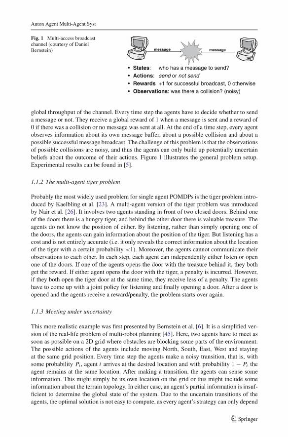
Fig. 1 Multi-access broadcastchannel (courtesy of DanielBernstein)
• States: who has a message to send?• Actions: send or not send• Rewards +1 for successful broadcast, 0 otherwise• Observations: was there a collision? (noisy)
message message
global throughput of the channel. Every time step the agents have to decide whether to senda message or not. They receive a global reward of 1 when a message is sent and a reward of0 if there was a collision or no message was sent at all. At the end of a time step, every agentobserves information about its own message buffer, about a possible collision and about apossible successful message broadcast. The challenge of this problem is that the observationsof possible collisions are noisy, and thus the agents can only build up potentially uncertainbeliefs about the outcome of their actions. Figure 1 illustrates the general problem setup.Experimental results can be found in [5].
1.1.2 The multi-agent tiger problem
Probably the most widely used problem for single agent POMDPs is the tiger problem intro-duced by Kaelbling et al. [23]. A multi-agent version of the tiger problem was introducedby Nair et al. [26]. It involves two agents standing in front of two closed doors. Behind oneof the doors there is a hungry tiger, and behind the other door there is valuable treasure. Theagents do not know the position of either. By listening, rather than simply opening one ofthe doors, the agents can gain information about the position of the tiger. But listening has acost and is not entirely accurate (i.e. it only reveals the correct information about the locationof the tiger with a certain probability <1). Moreover, the agents cannot communicate theirobservations to each other. In each step, each agent can independently either listen or openone of the doors. If one of the agents opens the door with the treasure behind it, they bothget the reward. If either agent opens the door with the tiger, a penalty is incurred. However,if they both open the tiger door at the same time, they receive less of a penalty. The agentshave to come up with a joint policy for listening and finally opening a door. After a door isopened and the agents receive a reward/penalty, the problem starts over again.
1.1.3 Meeting under uncertainty
This more realistic example was first presented by Bernstein et al. [6]. It is a simplified ver-sion of the real-life problem of multi-robot planning [45]. Here, two agents have to meet assoon as possible on a 2D grid where obstacles are blocking some parts of the environment.The possible actions of the agents include moving North, South, East, West and stayingat the same grid position. Every time step the agents make a noisy transition, that is, withsome probability Pi , agent i arrives at the desired location and with probability 1 − Pi theagent remains at the same location. After making a transition, the agents can sense someinformation. This might simply be its own location on the grid or this might include someinformation about the terrain topology. In either case, an agent’s partial information is insuf-ficient to determine the global state of the system. Due to the uncertain transitions of theagents, the optimal solution is not easy to compute, as every agent’s strategy can only depend
123

Auton Agent Multi-Agent Syst
Fig. 2 Meeting underuncertainty on a grid (courtesy ofDaniel Bernstein)
on some belief about the other agent’s location. An optimal solution for this problem is asequence of moves for each agent such that the expected time taken to meet is as low aspossible. Figure 2 shows a sample problem involving an 8×8 grid. Experimental results canbe found in [20].
1.2 Outline
We have described three examples of problems involving decentralized control of multipleagents. It is remarkable that prior to 2000, the computational complexity of these problemshad not been established, and no optimal algorithms were available. In Sects. 2.1 and 2.2,four different proposed formal models for this class of problems are presented and comparedwith one another. Equivalence of all these models in terms of expressiveness and complexityis established in Sect. 2.3. In Sect. 2.4, another formal model for describing decentralizedproblems is presented—one orthogonal to the others. This framework differs from the onespresented earlier as regards both expressiveness and computational complexity. Sect. 2.5goes on to consider interesting sub-classes of the general problem that lead to lower com-plexity classes. Some of these sub-problems are computationally tractable. Unfortunately,many interesting problems do not fall into one of the easy sub-classes, leading to the develop-ment of non-trivial optimal algorithms for the general class, which are described in Sect. 3.This is followed by a description of general approximation techniques in Sects. 4–6. Forsome approaches, specific limitations are identified and discussed in detail. In Sect. 7, all thepresented algorithms are compared along with their advantages and drawbacks. Finally, inSect. 8, conclusions are drawn and a short overview of open research questions is given.
2 Decision-theoretic models for multi-agent planning
To formalize the problem of decentralized control of multiple agents, a number of differ-ent formal models have recently been introduced. In all of these models, at each step, eachagent takes an action, a state transition occurs, and each agent receives a local observa-tion. Following this, the environment generates a global reward that depends on the set ofactions taken by all the agents. Figure 3 gives a schematic view of a decentralized processwith two agents. It is important to note that each agent receives an individual observation,but the reward generated by the environment is the same for all agents. Thus, we focus oncooperative systems in which each agent wants to maximize a joint global reward function. Incontrast, non-cooperative multi-agent systems, such as partially observable stochastic games(POSGs), allow each agent to have its own private reward function. Solution techniques for
123

Auton Agent Multi-Agent Syst
Fig. 3 Schematic view of adecentralized process with 2agents, a global reward functionand private observation functions(courtesy of Christopher Amato)
Table 1 Overview of formal models for decentralized control of multiple agents
Implicit belief representation Explicit beliefrepresentation
Implicitcommunication
DEC-POMDP (Sect. 2.1.1) MTDP (Sect. 2.1.2) I-POMDP(Sect. 2.4.1)
Explicitcommunication
DEC-POMDP-COM (Sect. 2.2.1) MTDP-COM (Sect. 2.2.2)
non-cooperative multi-agent systems are quite different from the algorithms described in thispaper and often rely on techniques from algorithmic game theory [28] and computationalmechanism design [34].
The five different formal models we will present in Sects. 2.1–2.4 can all be used to solvethe general problem as introduced via the examples in Sect. 1.1. One important aspect thatdifferentiates them is the treatment of communication. Some frameworks explicitly modelthe communication actions of the agents and others subsume them under the general actionsets. Each approach has different advantages and disadvantages, depending on the focus ofthe analysis. A second aspect that differentiates the models is whether they use an implicitor explicit representation of agent beliefs. An overview of the models is given in Table 1.
We begin with two formal models without explicit communication, followed by twoframeworks that explicitly model communication actions. We prove that all four models areequivalent in terms of expressiveness as well as computational complexity.
2.1 Models without explicit communication
2.1.1 The DEC-POMDP model
Definition 1 (DEC-POMDP) A decentralized partially observable Markov decision process(DEC-POMDP) is a tuple 〈I, S, {Ai}, P , {�i},O,R, T 〉 where
• I is a finite set of agents indexed 1, . . . , n.• S is a finite set of states, with distinguished initial state s0.• Ai is a finite set of actions available to agent i and �A = ⊗i∈IAi is the set of joint actions,
where �a = 〈a1, . . . , an〉 denotes a joint action.• P : S × �A→ �S is a Markovian transition function. P(s′|s, �a) denotes the probability
that after taking joint action �a in state s a transition to state s′ occurs.• �i is a finite set of observations available to agent i and �� = ⊗i∈I�i is the set of joint
observation, where �o = 〈o1, . . . , on〉 denotes a joint observation.
123
Auton Agent Multi-Agent Syst
• O : �A × S → � �� is an observation function. O(�o|�a, s′) denotes the probability ofobserving joint observation �o given that joint action �a was taken and led to state s′. Heres′ ∈ S, �a ∈ �A, �o ∈ ��.• R : �A × S → � is a reward function. R(�a, s′) denotes the reward obtained after joint
action �a was taken and a state transition to s′ occurred.• If the DEC-POMDP has a finite horizon, that horizon is represented by a positive integerT .
This framework was first proposed by Bernstein et al. [8]. In 2002, they introduced anotherversion of this model [6] that allows for more general observation and reward functions thatdifferentiate between different originating states. However, these more general functions caneasily be simulated in the original model by growing the state space to the cross product of Swith itself. Here, the earlier definition is used, because it simplifies showing the equivalencewith the MTDP model (see Theorem 1).
Definition 2 (Local policy for a DEC-POMDP) A local policy for agent i, δi , is a mappingfrom local histories of observations oi = oi1 . . . oit over �i to actions in Ai , δi : �∗i → Ai .
Definition 3 (Joint policy for a DEC-POMDP) A joint policy, δ = 〈δ1, . . . , δ2〉, is a tupleof local policies, one for each agent.
Solving a DEC-POMDP means finding a joint policy that maximizes the expected totalreward. This is formalized by the following performance criteria.
Definition 4 (Solution value for a finite-horizon DEC-POMDP) For a finite-horizon prob-lem, the agents act for a fixed number of steps, which is called the horizon and denoted byT . The value of a joint policy δ for a finite-horizon DEC-POMDP with initial state s0 is
V δ(s0) = E[T−1∑t=0
R(�at , st )|s0, δ].
When the agents operate over an unbounded number of time-steps or the time horizon isso large that it can best be modeled as being infinite, we use the infinite-horizon discountedperformance criterion. In this case, a discount factor, γ t , is used to weigh the reward collectedt time-steps into the future. For a detailed discussion of infinite-horizon models see Bernstein[5].
Definition 5 (Solution value for an infinite-horizon DEC-POMDP) The value of a joint pol-icy δ for an infinite-horizon DEC-POMDP with initial state s0 and discount factor γ ∈ [0, 1)is
V δ(s0) = E[ ∞∑t=0
γ tR(�at , st )|s0, δ].
All the models presented in this section can be used for finite-horizon or infinite-horizonproblems. However, for the introduction of the following formal models we will use the finite-horizon version because this is the version needed to prove the main complexity result inSect. 2.3.2. Note that, as for DEC-POMDPs, the infinite-horizon version of the other modelsonly differ from their finite-horizon counterparts in that they do not have the parameter T butinstead a discount factor γ . We will differentiate explicitly between the two versions when wepresent solution algorithms later because representation of policies and solution techniquesin general can differ significantly for finite and infinite-horizon problems respectively.
123

Auton Agent Multi-Agent Syst
2.1.2 The MTDP model
In 2002, Pynadath and Tambe [39] presented the MTDP framework, which is very similar tothe DEC-POMDP framework. The model as presented below uses one important assumption:
Definition 6 (Perfect recall) An agent has perfect recall if it has access to all of its receivedinformation (this includes all local observations as well as messages from other agents).
Definition 7 (MTDP) A multiagent team decision problem (MTDP) is a tuple 〈α, S,Aα,P,�α, Oα, Bα, R, T 〉, where
• α is a finite set of agents, numbered 1, . . . , n.• S = �1 × · · · × �m is a set of world states, expressed as a factored representation
(a cross product of separate features).• {Ai}i∈α is a set of actions for each agent, implicitly defining a set of combined actions,
Aα ≡ �i∈αAi .• P : S × Aα × S → [0, 1] is a probabilistic distribution over successor states, given the
initial state and a joint action, i.e. P(s, a, s′) = Pr(St+1 = s′|St = s,Atα = a).• {�}i∈α is a set of observations that each agent i can experience, implicitly defining a set
of combined observations, �α ≡ �i∈α�i .• Oα is a joint observation function modeling the probability of receiving a joint observation
ω after joint action a was taken and a state transition to s′ occurred, i.e. Oα(s′, a, ω) =
Pr(�t+1α = ω|St+1 = s′,Atα = a).
• Bα is the set of possible combined belief states. Each agent i ∈ α forms a belief statebti ∈ Bi , based on its observations seen through time t , where Bi circumscribes the setof possible belief states for agent i. This mapping of observations to belief states is per-formed by a state estimator function under the assumption of perfect recall. The resultingcombined belief state is denoted Bα ≡ �i∈αBi . The corresponding random variable btαrepresents the agents’ combined belief state at time t .• R : S × Aα → � is a reward function representing a team’s joint preferences.• If the MTDP has a finite horizon, that horizon is represented by a positive integer T .
Note that due to the assumption of perfect recall, the definition of the state estimator func-tion is not really necessary as in that case it simply creates a list of observations. However,if this assumption is relaxed or a way of mapping observations to a compact belief stateis found, this additional element might become useful. So far, no state estimator functionwithout perfect recall has been proposed, and no compact representation of belief states formulti-agent settings has been introduced.
Definition 8 (Domain-level policy for an MTDP) The set of possible domain-level policiesin an MTDP is defined as the set of all possible mappings from belief states to actions,πiA : Bi → Ai .
Definition 9 (Joint domain-level policy for an MTDP) A joint domain-level policy for anMTDP, παA = 〈π1A, . . . , πnA〉, is a tuple of domain-level policies, one for each agent.
Solving an MTDP means finding a joint policy that maximizes the expected global reward.
2.1.3 Computational complexity and equivalence results
Before the equivalence of the DEC-POMDP model and the MTDP model can be established,the precise notion of equivalence must be defined. This requires a short excursion to com-plexity theory. All models presented in this paper so far describe decentralized optimization
123

Auton Agent Multi-Agent Syst
problems. Thus, finding a solution for those problems means finding a policy that maximizesthe expected value. However, most complexity classes are defined in terms of decision prob-lems. A decision problem is a formal question with a “yes/no” answer, or equivalently it isthe set of problem instances where the answer to the question is “yes”. A complexity class isthen defined by the set of all decision problems that it contains. Alternatively, a complexityclass can also be defined by a complexity measure (e.g. time, space) and a correspondingresource bound (e.g. polynomial, exponential). P for example denotes the complexity classthat contains all decision problems that can be solved in polynomial time.
All models/problems presented in this paper can be converted to “yes/no” decision prob-lems to analyze their complexity. This is done by adding a parameterK to denote a thresholdvalue. For example, the decision problem for a DEC-POMDP then becomes: given DEC-POMDP 〈I, S, {Ai}, P , {�i},O,R, T ,K〉, is there a joint policy for which the value of theinitial state s0 exceedsK? Obviously, actually finding the optimal policy for a DEC-POMDPproblem can be no easier than the threshold problem. Note that for all equivalence proofs inthis paper we are reducing decision problems to each other.
In Sect. 2.3.2 we will show that the DEC-POMDP decision problem is NEXP-complete,i.e. it can be solved in nondeterministic exponential time and every other problem in NEXPcan be efficiently reduced to this problem, where here “efficiently” means in polynomial time.More formally this means: DEC-POMDP ∈ NEXP and ∀C ∈ NEXP: C ≤p DEC-POMDP.For more details on complexity theory see Papadimitriou [31].
Definition 10 (Equivalence of models/problems) Two models are called equivalent if theircorresponding decision problems are complete for the same complexity class.
To show that two problems are equivalent, a completeness proof such as in Sect. 2.3.2could be performed for both problems. Alternatively, formal equivalence can be proved byshowing that the two problems are reducible to each other. To reduce decision problem A todecision problemB, a function f has to be found that formally defines a mapping of probleminstances x ∈ A to problem instances f (x) ∈ B, such that the answer to x is “yes” if and onlyif the answer to f(x) is “yes.” This mapping-function f has to be computable in polynomialtime. The reduction of problem A to problem B in polynomial time is denoted A ≤p B.
Note that this notion of equivalence implies that if two models are equivalent they areequivalent in terms of expressiveness as well as in terms of complexity. That is, the frame-works can describe the same problem instances and are complete for the same complexityclass. To know the complexity class for which they are complete, at least one completenessproof for one of the models has to be obtained. Any framework for which equivalence withthis model has been shown is then complete for the same complexity class.
Theorem 1 The DEC-POMDP model and the MTDP model are equivalent under the perfectrecall assumption.
Proof We need to show: 1. DEC-POMDP ≤p MTDP and 2. MTDP ≤p DEC-POMDP.
1. DEC-POMDP ≤p MTDP:A DEC-POMDP decision problem is a tuple 〈I, S, {Ai}, P , {�i},O,R, T ,K〉 and anMTDP decision problem is a tuple 〈α, S′,Aα, P ′,�α, Oα, Bα, R′, T ′,K ′〉. There is anobvious mapping between:
• the finite sets of agents, I = α.• the finite set of world states, S = S′.• the finite set of joint actions for each agent, �A = Aα .
123

Auton Agent Multi-Agent Syst
• the probability table for state transitions, P(s′|s, �a) = P ′(s, a, s′).• the finite set of joint observations, �� = �α .• the observation function, O(�o|�a, s′) = Oα(s, a, ω).• the reward function, R(�a, s′) = R′(a, s).• the finite horizon parameter, T = T ′.• the threshold parameter, K = K ′.
The possible local histories of observations available to the agents in a DEC-POMDPare mapped to the possible belief states bti of the MTDP, i.e. bti is simply the sequence ofobservations of agent i until time t . Finding a policy for an MTDP means finding a map-ping from belief states to actions. Thus, a policy for the resulting MTDP that achievesvalueK also constitutes a policy for the original DEC-POMDP with valueK , where thefinal policies are mappings from local histories of observations to actions.
2. MTDP ≤p DEC-POMDP:For α, S′, Aα, P ′, �α, Oα, R′, T ′, K ′, the same mapping as in part 1 is used. Theonly remaining element is the set of possible combined belief states, Bα . In an MTDP,each agent forms its belief state, bti ∈ Bi , based on its observations seen through time t .Due to the perfect recall assumption in the MTDP model, the agents recall all of theirobservations. Thus, their belief states represent their entire histories as sequences ofobservations. Obviously, with this restriction, the state estimator function and the beliefstate space of the MTDP do not add anything beyond the DEC-POMDP model. Thus,the history of observations can simply be extracted from the belief state and then theresulting DEC-POMDP can be solved, i.e. a policy that is a mapping from histories ofobservations to actions can be found. Thus, a solution with valueK for the DEC-POMDPexists if and only if a solution with value K for the original MTDP exists.
Therefore, the DEC-POMDP model and the MTDP model are equivalent. ��It becomes apparent that the only syntactical difference between MTDPs and DEC-
POMDPs is the additional state estimator function and the resulting belief state of the MTDPmodel. But, with the assumption that the agents have perfect recall of all of their observa-tions, the resulting belief state is nothing but a sequence of observations and therefore existsimplicitly in a DEC-POMDP, too. We prefer the DEC-POMDP notation because it is some-what cleaner and more compact. Therefore, from now on we use the DEC-POMDP as the“standard” model for decentralized decision making.
2.2 Models with explicit communication
Both models presented in Sect. 2.1 have been extended with explicit communication actions.In the resulting two models, the interaction among the agents is a process in which agentsperform an action, then observe their environment and send a message that is instantaneouslyreceived by the other agents (no delays in the system). Both models allow for a general syntaxand semantics for communication messages. Obviously, the agents need to have conventionsabout how to interpret these messages and how to combine this information with their ownlocal information. One example of a possible communication language is i = �i , wherethe agents simply communicate their observations.
This distinction between the two different types of actions might seem unnecessary forpractical applications but it is useful for analytical examinations. It provides us with a bet-ter way to analyze the effects of different types of communication in a multi-agent setting(cf. [19]).
123

Auton Agent Multi-Agent Syst
2.2.1 The DEC-POMDP-COM model
The following model is equivalent to the one described in Goldman and Zilberstein [18]. Theformal definition of some parts have been changed to make the DEC-POMDP-COM modelpresented here a straightforward extension of the previously described DEC-POMDP model.
Definition 11 (DEC-POMDP-COM) A decentralized partially observable Markov decisionprocess with communication (DEC-POMDP-COM) is a tuple 〈I, S, {Ai}, P , {�i},O,,C,RA,R, T 〉 where:
• I, S, {Ai}, P , {�i}, O, and T are defined as in the DEC-POMDP.• is the alphabet of communication messages. σi ∈ is an atomic message sent by
agent i, and �σ = 〈σ1, . . . , σn〉 is a joint message, i.e. a tuple of all messages sent by theagents in one time step. A special message belonging to is the null message, εσ , whichis sent by an agent that does not want to transmit anything to the others.
• C : → � is the message cost function. C(σi) denotes the cost for transmittingatomic message σi . We set C(εσ ) = 0, i.e. agents incur no cost for sending a nullmessage.
• RA : �A × S → � is the action reward function identical to the reward function in aDEC-POMDP, i.e. RA(�a, s′) denotes the reward obtained after joint action �a was takenand a state transition to s′ occurred.
• R : �A × S × � → � denotes the total reward function, defined via RA and C :R(�a, s′, �σ) = RA(�a, s′)−∑
i∈I C(σi).
Note that if R is represented explicitly, the representation size of R is at least �(||n). IfR is only represented implicitly via RA and C , we will assume that || is polynomiallybounded by either |�i | or |Ai |, which implies that the observation functionO will be of sizeat least �(||n).
Definition 12 (Local policy for action for a DEC-POMDP-COM) A local policy for actionfor agent i, δAi , is a mapping from local histories of observations oi over �i and histories ofmessages σj received (j �= i) to control actions in Ai , δAi : �∗i × �∗ → Ai .
Definition 13 (Local Policy for communication for a DEC-POMDP-COM) A local policyfor communication for agent i, δi , is a mapping from local histories of observations oiover �i , and histories of messages σ j received (j �= i) to communication actions in ,δi : �∗i × �∗ → .
Definition 14 (Joint policy for a DEC-POMDP-COM) A joint policy δ = 〈δ1, . . . , δn〉 is atuple of local policies, one for each agent, where each δi is composed of the communicationand action policies for agent i.
Solving a DEC-POMDP-COM means finding a joint policy that maximizes theexpected total reward, over either an infinite or a finite horizon. See Goldman and Zilberstein[18] for further discussion.
Theorem 2 The DEC-POMDP model and the DEC-POMDP-COM model are equivalent.
Proof We need to show: 1. DEC-POMDP ≤p DEC-POMDP-COM and 2. DEC-POMDP-COM ≤p DEC-POMDP.
123
Auton Agent Multi-Agent Syst
1. DEC-POMDP ≤p DEC-POMDP-COM:For the first reduction, a DEC-POMDP can simply be mapped to a DEC-POMDP-COMwith an empty set of communication messages and no cost function for the communi-cation messages. Thus, = ∅ and C is the empty function. Obviously a solution withvalue K for the resulting DEC-POMDP-COM is also a solution with value K for theoriginal DEC-POMDP.
2. DEC-POMDP-COM ≤p DEC-POMDP:The DEC-POMDP-COM decision problem is a tuple 〈I, S, {Ai}, P , {�i},O,,C,RA,R, T ,K〉 and a DEC-POMDP decision problem is a tuple 〈I ′, S′, {Ai}′, P ′, {�i}′,O ′, R′, T ′,K ′〉. The only difference between these models is the explicit modeling of thecommunication actions in the DEC-POMDP-COM model, but those can be simulatedin the DEC-POMDP in the following way:
• The size of the state set S′ has to be doubled to simulate the interleaving of controlactions and communication actions. Thus, S′ = S × {0, 1}. Here, 〈s, 0〉 representsa system state where only control actions are possible, denoted a control state. And〈s, 1〉 represents a system state where only communication actions are possible,denoted a communication state.• The length of the horizon is doubled, i.e. T ′ = 2 · T , to account for the fact that
for every time step in the original DEC-POMDP-COM we now have two time steps,one for the control action and one for the communication action.• Each communication message is added to the action sets: {Ai}′ = {Ai} ∪ . To
differentiate control actions from communication actions, joint control actions aredenoted �a and joint communication actions are denoted �σ .• For each possible joint communication message, one new joint observation is added
to the joint observation set: ��′ = �� ∪n. Thus, the observation function has to bedefined for consistent joint messages/observations only, i.e. where every agent hasinformation about the same nmessages (1 sent and n−1 received). Note that we cando this mapping only because message transmission is deterministic. Alternatively,adding n-tuples of single-agent observations consisting of n− 1 received messageswould contain redundant information and, more importantly, could not be done inpolynomial time. Although this simpler mapping is still exponential in n, it can bedone in time polynomial in the input size, because according to the definition of aDEC-POMDP-COM the representations of R or O are of size at least �(||n). Inthe following, we let o denote a normal observation and �σ denote an observationrepresenting n communication messages from all agents.• The transition function P ′ is constructed in such a way that if the agents are in a
control state, every joint control action leads to a communication state. Similarly, ifthe agents are in a communication state, every joint communication action leads to acontrol state. The transition probabilities for a control action taken in a control stateare implicitly defined by the original transition function. A communication actiontaken in a communication state deterministically leads to a successor state whereonly the second component of the state changes from 1 to 0. More formally:
∀s, s′, �a : P ′(〈s′, 1〉|〈s, 0〉, �a) = P(s′|s, �a)∀s, �σ−i : P ′(〈s, 0〉|〈s, 1〉, �σ−i ) = 1
The transition function must be 0 for all impossible state transitions. This includesa control action taken in a control state leading to another control state, a communi-cation action taken in a communication state but leading to a successor state where
123

Auton Agent Multi-Agent Syst
the first component of the state also changes, and a communication action taken ina communication state leading to a communication state again. More formally:
∀s, s′, �a : P ′(〈s′, 0〉|〈s, 0〉, �a) = 0
∀s′ �= s, �σ−i : P ′(〈s′, 0〉|〈s, 1〉, �σ−i ) = 0
∀s, s′, �σ−i : P ′(〈s′, 1〉|〈s, 1〉, �σ−i ) = 0
Furthermore, the transition function has to be defined for the cases of actions notpossible in the original model, i.e. when a communication action is taken in a controlstate or when a control action is taken in a communication state. In these cases thestate must simply remain the same. More formally:
∀s = s′, �σ−i : P ′(〈s′, 0〉|〈s, 0〉, �σ−i ) = 1
∀s �= s′, �σ−i : P ′(〈s′, 0〉|〈s, 0〉, �σ−i ) = 0
and
∀s, s′, �σ−i : P ′(〈s′, 1〉|〈s, 0〉, �σ−i ) = 0
∀s = s′, �a : P ′(〈s′, 1〉|〈s, 1〉, �a) = 1
and
∀s �= s′, �a : P ′(〈s′, 1〉|〈s, 1〉, �a) = 0
∀s, s′, �a : P ′(〈s′, 0〉|〈s, 1〉, �a) = 0
Note that with this definition of the transition function P ′, the agents could theo-retically now make time go by without really taking any actions, e.g. by taking acommunication action in a control state. We will prevent this by adjusting the rewardfunction accordingly.• The observation functionO ′ has to be defined for control actions and for communi-
cation actions. The observation probabilities for a control action taken in a controlstate are implicitly defined by the original observation function. As explained above,for communication states we use the simplification that each joint communicationaction corresponds to only one joint observation consisting of n messages (whichis possible due to the deterministic message transmission). Thus, the observationfunction has to be defined such that after taking a joint communication action �σ theprobability of observing the corresponding joint communication message is 1 andthe probability of observing any other observation is 0. Thus:
∀�a, s′, �o : O ′(�o|�a, 〈s′, 1〉) = O(�o|�a, s′)
and
∀�o, �σ , s′ : O ′(�o|�σ, 〈s′, 0〉) ={
1 if �o = �σ0 else
For completeness, the observation function must be defined for all impossible action-state combinations. One simple way to do this is to set the observation probabilityequal to 1 for observing �εσ , the joint message only consisting of null messages, andto set all other observation probabilities equal to 0. More formally:
123
Auton Agent Multi-Agent Syst
∀�o, �σ, s′ : O ′(�o|�σ, 〈s′, 1〉) ={
1 if �o = �εσ0 else
and
∀�o, �a, s′ : O ′(�o|�a, 〈s′, 0〉) ={
1 if �o = �εσ0 else
Again, although we are adding O(||n) joint observations to the observation func-tion, this mapping can be done in time polynomial in the input size, because accordingto the definition of a DEC-POMDP-COM the representations of R or O are of sizeat least �(||n).• The reward function R′ has to be changed to account for the communication costs
as defined by C . If 〈s′, 0〉 is the control state reached after joint communicationaction �σ = 〈σ1, . . . σn〉 was taken, then the reward must represent the sum of thecommunication costs C(σi). For control actions taken in a control state, the rewardis defined implicitly via the original reward function. More formally:
∀�σ, s′ : R′(�σ, 〈s′, 0〉) =n∑i
C(σi)
and
∀�a, s′ : R′(�a, 〈s′, 1〉) = RA(�a, s′)Again, for completeness the reward function has to be defined for impossible action-state combinations. For those cases we have made sure that the agents simply stayin the same state and observe the null message. Unfortunately, if the original DEC-POMDP-COM was constructed such that for certain (or all) state transitions theagents received a negative reward, finding an optimal plan in the new DEC-POMDPwould result in an undesired solution. The optimal plan might include steps where anagent takes a “null action” by choosing an impossible state-action combination. Toprevent this from happening, we set the reward to negative infinity whenever a controlaction leads to a control state or a communication action leads to a communicationstate. Thus:
∀�a, s′ : R′(�a, 〈s′, 0〉) = −∞and
∀�σ, s′ : R′(�σ , 〈s′, 1〉) = −∞In the resulting DEC-POMDP, the agents start off taking a joint control action. Thena state transition to a communication state occurs. After taking a joint communicationaction, a state transition to a control state occurs. This corresponds exactly to the courseof action in the original DEC-POMDP-COM where the agents also had designatedaction and communication phases. Receiving messages is simulated by observationsthat correspond to the joint messages. Therefore, the information available to an agent inthe DEC-POMDP is the same as in the original DEC-POMDP-COM. By constructingP ′,O ′ and R′ appropriately, we ensure that a policy with value K can be found forthe resulting DEC-POMDP if and only if a policy with value K can be found for the
123

Auton Agent Multi-Agent Syst
original DEC-POMDP-COM. This completes the reduction of a DEC-POMDP-COMto a DEC-POMDP.
Thus, the DEC-POMDP and the DEC-POMDP-COM models are equivalent. ��
2.2.2 The COM-MTDP model
Definition 15 (COM-MTDP)1 A communicative multiagent team decision problem (COM-MTDP) is a tuple 〈α, S,Aα, P,�α, Oα,�α, Bα, R〉, where
• α, S, Aα, P, �α , and Oα remain defined as in an MTDP.• �α is a set of combined communication messages, defined by �α ≡ �i∈αi , where{i}i∈α is a set of possible messages for each agent i.• Bα is an extended set of possible combined belief states. Each agent i ∈ α forms belief
state bti ∈ Bi , based on its observations and on the messages received from the otheragents. This mapping of observations and messages to belief states is performed by thestate estimator function under the assumption of perfect recall.• R is an extended reward function, now also representing the cost of communicative acts.
It is defined by R : S × Aα ×�α → �.
As with MTDPs, in COM-MTDPs, the state estimator function does not add any additionalfunctionality due to the assumption of perfect recall. However, if this assumption is relaxed,a state estimator has the potential to model any noise or temporal delays that might occur inthe communication channel. Furthermore, it could possibly perform some preprocessing ofthe observations and messages. So far, no such state estimators have been proposed.
Definition 16 (Communication policy for a COM-MTDP) A communication policy for aCOM-MTDP is a mapping from the extended belief state space to communication messages,i.e. πi : Bi → i .
Definition 17 (Joint communication policy for a COM-MTDP) A joint communication pol-icy for an MTDP-COM, πα = 〈π1, . . . , πn〉, is a tuple of communication policies, onefor each agent.
Definition 18 (Joint policy for a COM-MTDP) A joint policy for a COM-MTDP is a pair,consisting of a joint domain-level policy and a joint communication policy, 〈πα,παA〉.
Solving a COM-MTDP means finding a joint policy that maximizes the expected totalreward over either an infinite or a finite horizon.
2.3 Consolidation of 4 different formal models
2.3.1 Equivalence results
Theorem 3 The DEC-POMDP-COM model and the COM-MTDP model are equivalentunder the perfect recall assumption.
Proof We need to show that: 1. DEC-POMDP-COM ≤p COM-MTDP and 2. COM-MTDP≤p DEC-POMDP-COM.
1 Adapted from Pynadath and Tambe [39].
123

Auton Agent Multi-Agent Syst
As has been shown in Theorem 1, the DEC-POMDP model and the MTDP model are equiva-lent. The extensions of these models introduce/change, C,RA andR for the DEC-POM-DP-COM model and �α, Bα , andR′ for the COM-MTDP model. For the parts of the modelsthat did not change, the same mapping as presented in the earlier proof is used.
1. DEC-POMDP-COM ≤p COM-MTDP:Again, there are obvious mappings between:
• The set of communication messages, = �α .• The extended reward function, R(�a, s′, �σ) = R′(a, s′, σ ).
The possible local histories of observations and communication messages received thatare available to the agent in a DEC-POMDP are mapped to the extended set of pos-sible combined belief states Bα of the COM-MTDP, i.e. bti is simply the sequence ofobservations and communication messages received by agent i until time t . Finding apolicy for a COM-MTDP means finding a mapping from the extended set of combinedbelief states to actions (domain level actions and communication actions). Thus, a policywith value K for the resulting COM-MTDP is at the same time a policy with value Kfor the original DEC-POMDP-COM, where the final policies are mappings from localhistories of observations and communication messages to actions (control actions andcommunication actions).
2. COM-MTDP ≤p DEC-POMDP-COM:For and R, the same mappings as in part 1 are used. The only remaining element isthe extended set of possible combined belief states, Bα , which again exists implicitly ina DEC-POMDP-COM, too. In a COM-MTDP, each agent forms its belief state, bti ∈ Bi ,based on its observations and the messages it has received up to time t . The extendedstate estimator function now forms the belief state with the following three operations:
(a) Initially, the belief state is an empty history.(b) Every new observation agent i receives is appended to its belief state.(c) Every new message agent i receives is also appended to its belief state.
Again, the COM-MTDP model assumes that the agents have perfect recall, i.e. they recallall of their observations and messages. Thus, the extended state estimator function buildsup a complete history of observations and messages as in a DEC-POMDP-COM. Thehistory of observations and communication messages can therefore simply be extractedfrom the belief state of the COM-MTDP and the resulting DEC-POMDP-COM can thenbe solved. This means finding a policy that is a mapping from histories of observationsand communication messages to actions. Thus, a solution to the DEC-POMDP-COMwith value K is also a solution to the original COM-MTDP with value K .
Therefore, the DEC-POMDP-COM and COM-MTDP models are equivalent. ��The following corollary now immediately follows from Theorems 1, 2 and 3.
Corollary 1 All of the aforementioned models (DEC-POMDP, DEC-POMDP-COM, MTDP,and COM-MTDP) are equivalent.
As explained in Sect. 2.1, we consider the DEC-POMDP model to be somewhat cleanerand more compact than the MTDP model. Obviously, the same holds true for DEC-POMDP-COMs versus COM-MTDPs. Whether one uses the model with or without explicit communi-cation messages depends on the specific purpose. The models are equivalent, but using one ofthe models might be advantageous for a particular analysis. For example, when analyzing the
123

Auton Agent Multi-Agent Syst
effects of different types of communication, the DEC-POMDP-COM model is more suitablethan the DEC-POMDP model (see for example [19]). If communication actions are takento be no different than any other action, the DEC-POMDP model is more compact and thusmore attractive.
2.3.2 Complexity results
The first complexity results for Markov decision processes go back to Papadimitriou and Tsi-tsiklis [33], where they showed that the MDP problem is P-complete and that the POMDPproblem is PSPACE-complete for the finite-horizon case. For a long time, no tight complexityresults for decentralized processes were known. In 1986, Papadimitriou and Tsitsiklis [32]proved that decentralized control of MDPs must be at least NP-hard; however, a completecomplexity analysis also giving tight upper bounds was still missing.
In 2000, Bernstein et al. [8] were the first to prove that DEC-POMDPs with a finite horizonare NEXP-complete. This was a breakthrough in terms of understanding the complexity ofdecentralized control of multiple agents. In particular, due to the fact that it has been proventhat P and EXP are distinct, this shows that optimal decentralized control of multiple agentsis infeasible in practice. Moreover, it is strongly believed by most complexity theorists thatEXP �= NEXP and that solving NEXP-complete problems needs double exponential timein the worst case. Note that this has not been proven formally, but for the remainder of thispaper it is assumed to be true.
Below, a sketch of the original proof is presented. Obviously, due to the equivalence resultsfrom Corollary 1, all complexity results obtained for DEC-POMDPs hold also for DEC-POMDP-COMs, MTDPs and COM-MTDPs. The complexity proof involves two agentsbecause this is sufficient to show NEXP-completeness. Let DEC-POMDPn denote a DEC-POMDP with n agents. In the finite-horizon version of the DEC-POMDP model, we assumethat T ≤ |S|. The theorems and proofs in this section are based on Bernstein et al. [6].
Theorem 4 For any n ≥ 2, a finite-horizon DEC-POMDPn ∈ NEXP.
Proof The following process shows that a non-deterministic Turing machine can solve anyinstance of a DEC-POMDPn in at most exponential time.
1. Guess a joint policy and write it down in exponential time. This is possible, because ajoint policy consists of nmappings from observation histories to actions. Since T ≤ |S|,the number of possible histories is exponentially bounded by the problem description.
2. The DEC-POMDP together with the guessed joint policy can be viewed as an exponen-tially bigger POMDP using n-tuples of observations and actions.
3. In exponential time, convert each of the exponentially many observation sequences intoa belief state.
4. In exponential time, compute transition probabilities and expected rewards for an expo-nentially bigger belief state MDP.
5. This MDP can be solved in polynomial time, which is exponential in the original problemdescription.
Thus, there is an accepting computation path in the non-deterministic machine if and only ifthere is a joint policy that can achieve reward K . ��
To present the full complexity result, we need to define a few additional properties. Notethat some of these properties have different names in the DEC-POMDP and MTDP frame-works. We provide both names below, but only the first one listed in each definition is usedin this paper.
123

Auton Agent Multi-Agent Syst
Definition 19 (Joint full observability≡ collective observability) A DEC-POMDP is jointlyfully observable if the n-tuple of observations made by all the agents uniquely determinesthe current global state. That is, if O(�o|�a, s′) > 0 then Pr(s′|�o) = 1.
Definition 20 (DEC-MDP) A decentralized Markov decision process (DEC-MDP) is aDEC-POMDP with joint full observability.
Note that in a DEC-MDP, each agent alone still only has partial observability and doesnot have full information about the global state.
Theorem 5 For any n ≥ 2, a finite-horizon DEC-MDPn is NEXP-hard.
Proof sketch The detailed proof of this lower bound is quite involved and can be found in Bern-stein et al. [6]. We include a sketch of the proof below. The proof is based on a reduction of aknown NEXP-complete problem called TILING to DEC-MDPn. A TILING problem instanceincludes a board of size n×n (the size n is represented compactly in binary), a set of tile typesL = {tile-0, . . . , tile-k}, and a set of binary horizontal and vertical compatibility relationsH,V ⊆ L×L. A tiling is a mapping f : {0, . . . , n−1}× {0, . . . , n−1} → L. A tiling f isconsistent if and only if (a) f (0, 0) =tile-0 and (b) for all x, y, 〈f (x, y), f (x + 1, y)〉 ∈ H ,and 〈f (x, y), f (x, y + 1)〉 ∈ V . The decision problem is to determine, given L, H, V , andn, whether a consistent tiling exists. Figure 4 shows an example of a tiling instance and acorresponding consistent tiling.
For the following reduction, a fixed but arbitrarily chosen instance of the tiling problemis assumed, i.e. L, H, V , and n are fixed. A corresponding DEC-MDP is constructed, withthe requirement that it is solvable (i.e. there is a joint policy for which the value of the initialstate s0 exceeds K) if and only if the selected tiling instance is solvable. The basic idea is tocreate a DEC-MDP where the agents are given tile positions from the environment in eachstep and then select tiles to fill the pair of positions in the next step. The environment thenchecks whether this leads to a consistent tiling.
A naive approach could lead to the creation of a state for every pair of tile positions.Unfortunately, this would result in an exponential blow-up in problem size, rather than apolynomial reduction. Thus, the environment itself cannot “remember” all the informationabout the process. As it turns out, it is sufficient to only remember information about therelative position of two tiles (whether the locations are the same, horizontally adjacent, or
Fig. 4 The tiling problem(courtesy of Daniel Bernstein)
123
Auton Agent Multi-Agent Syst
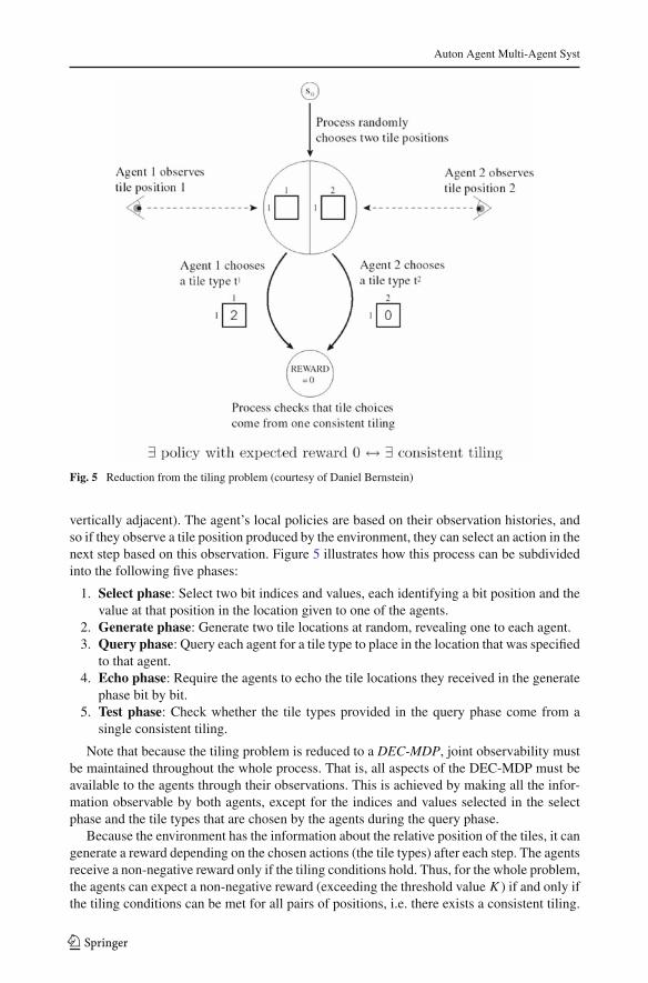
Fig. 5 Reduction from the tiling problem (courtesy of Daniel Bernstein)
vertically adjacent). The agent’s local policies are based on their observation histories, andso if they observe a tile position produced by the environment, they can select an action in thenext step based on this observation. Figure 5 illustrates how this process can be subdividedinto the following five phases:
1. Select phase: Select two bit indices and values, each identifying a bit position and thevalue at that position in the location given to one of the agents.
2. Generate phase: Generate two tile locations at random, revealing one to each agent.3. Query phase: Query each agent for a tile type to place in the location that was specified
to that agent.4. Echo phase: Require the agents to echo the tile locations they received in the generate
phase bit by bit.5. Test phase: Check whether the tile types provided in the query phase come from a
single consistent tiling.
Note that because the tiling problem is reduced to a DEC-MDP, joint observability mustbe maintained throughout the whole process. That is, all aspects of the DEC-MDP must beavailable to the agents through their observations. This is achieved by making all the infor-mation observable by both agents, except for the indices and values selected in the selectphase and the tile types that are chosen by the agents during the query phase.
Because the environment has the information about the relative position of the tiles, it cangenerate a reward depending on the chosen actions (the tile types) after each step. The agentsreceive a non-negative reward only if the tiling conditions hold. Thus, for the whole problem,the agents can expect a non-negative reward (exceeding the threshold valueK) if and only ifthe tiling conditions can be met for all pairs of positions, i.e. there exists a consistent tiling.
123

Auton Agent Multi-Agent Syst
Thus, a solution for the DEC-MDPn at the same time constitutes a solution to the tilingproblem. Accordingly, since the tiling problem is NEXP-complete, solving a finite-horizonDEC-MDPn is NEXP-hard. ��Corollary 2 For any n ≥ 2, DEC-POMDPn is NEXP-hard.
Proof Because the set of all DEC-POMDPs is a true superset of the set of all DEC-MDPs,this follows immediately from Theorem 5. ��
Because all four formal models for optimal multi-agent planning are equivalent, the lastcomplexity result also holds for DEC-POMDP-COMs, MTDPs and COM-MTDPs. Thus, infuture research, any one of the models can be used for purposes of theoretical analysis, aswell as for the development of algorithms. The results will always apply to the other modelsas well. Note that we have only analyzed the complexity of finite-horizon problems in thissection. This is because the situation is significantly different for the infinite-horizon case.In 1999, Madani et al. [25] showed that infinite-horizon POMDPs are undecidable. Thus,because a DEC-POMDP with one agent reduces to a single-agent POMDP, it is obvious thatinfinite-horizon DEC-POMDPs are also undecidable.
2.3.3 Approximation and complexity
The notion of equivalence used so far means that the decision problem versions of all fourmodels have the same worst-case complexity. However, it does not immediately imply any-thing about the approximability of their corresponding optimization problems. An under-standing of this approximability is nevertheless desirable in light of the high worst-casecomplexity. The standard polynomial time reductions we have used are inadequate to showequivalence of two optimization problems in terms of approximability. Two problems A andB may be equivalent in terms of worst-case complexity, but it can still be conceivable that Ahas an efficient approximation algorithm while B does not.
A more careful kind of reduction that preserves approximability is called an L-Reduction.Showing that there exists an L-reduction from optimization problem A to optimization prob-lem B when there exists an approximation algorithm for B implies that there also exists anapproximation algorithm for A. The formal details of this reduction technique are beyondthe scope of this paper (see Papadimitriou [31, chap. 13] for a detailed discussion of thistopic). However, we can give some intuition and an informal proof of why the four modelsconsidered here are also equivalent in terms of approximability.
First, we use the result shown by Rabinovich et al. [40] in 2003 that even ε-optimal his-tory-dependent joint policies are still NEXP-hard to find in DEC-POMDPs. In other words,DEC-POMDPs are not efficiently approximable. As the DEC-POMDP-COM model is astraightforward extension of the DEC-POMDP model, DEC-POMDP-COMs are also notefficiently approximable. An analogous argument holds for the MTDP and the MTDP-COMmodel. If the MTDP model is not efficiently approximable the same would hold true forthe MTDP-COM model. Thus, it suffices to show that there is an L-reduction from theDEC-POMDP model to the MTDP model.
Looking at the reduction used in Sect. 2.1.3, we can observe that we used a very easy one-to-one mapping of the elements of a DEC-POMDP to the resulting MTDP. Most importantly,this mapping can be done in logarithmic space, one of the main requirements of L-reduc-tions. A second requirement is that the solution for the resulting MTDP can be transformedinto a solution for the original DEC-POMDP using logarithmic space. As we have noted
123

Auton Agent Multi-Agent Syst
before, a solution to the resulting MTDP is at the same time a solution to the original DEC-POMDP with the same solution value, and thus this requirement is trivially fulfilled. The lastrequirement of L-reductions concerns the optimal values of the two problem instances—theoriginal DEC-POMDP and the MTDP resulting from the mapping. The optimal solutionsfor both instances must be within some multiplicative bound of each other. Again, becausethe solutions for the two problem instances will actually have the exact same value, this lastrequirement of the L-reduction is also fulfilled, and we have shown that MTDPs are not effi-ciently approximable. Thus, all four models are also equivalent in terms of approximability;finding ε-approximations for them is NEXP hard.
2.4 Models with explicit belief representation
In this section, a different approach to formalize the multi-agent planning problem is pre-sented. The approach proves to be fundamentally different from the models presented in theprevious sections, in terms of both expressiveness and complexity.
Single-agent planning is known to be P-complete for MDPs and PSPACE-complete forPOMDPs. The unfortunate jump in complexity to NEXP when going from 1 to 2 agentsis due to the fact that in the DEC-POMDP model there is probably no way of compactlyrepresenting a policy (see also Sect. 2.5.2 for further discussion of this topic). Agents mustremember their complete histories of observations, resulting in exponentially large policies.If there were a way to construct a compact belief state about the whole decentralized process,one could hope to get a lower complexity than NEXP. For each agent, this would include notonly expressing a belief about its own local state, but also its belief about the other agents(their states, their policies, etc.). Such belief states are a central component of the I-POMDPmodel introduced by Gmytrasiewicz and Doshi [16]. This framework for sequential planningin partially observable multi-agent systems is even more expressive than the DEC-POMDPmodel, as it allows for non-cooperative as well as cooperative settings. Thus, it is closelyrelated to partially observable stochastic games (POSGs). In contrast to classical game the-ory, however, this approach does not search for equilibria or other stability criteria. Instead, itfocuses on finding the best response action for a single agent with respect to its belief aboutthe other agents, thereby avoiding the problems of equilibria-based approaches, namely theexistence of multiple equilibria.
The formal I-POMDP model and corresponding solution techniques are presented below.In Sect. 2.4.3, we examine its complexity and in Sect. 2.4.4, we discuss the applicability ofthis model and its relationship to DEC-POMDPs.
2.4.1 The I-POMDP model
I-POMDPs extend the POMDP model to the multi-agent case. Now, in addition to a beliefover the underlying system state, a belief over the other agents is also maintained. To modelthis richer belief, an interactive state space is used. A belief over an interactive state sub-sumes the belief over the underlying state of the environment as well as the belief over theother agents. Notice that—even if just two agents are considered—expressing a belief overanother agent might include a belief over the other agent’s belief. As the second agent’s beliefmight also include a belief over the first agent’s belief, this technique leads to a nesting ofbeliefs which makes finding optimal solutions within this model problematic. This topic isdiscussed later in Sects. 2.4.3 and 2.4.4.
123
Auton Agent Multi-Agent Syst
To capture the different notions of beliefs formally, some definitions have to be introduced.The nesting of beliefs then leads to the definition of finitely nested I-POMDPs in the nextsection.
Definition 21 (Frame) A frame of an agent i is θi = 〈Ai,�i, Ti,Oi, Ri,OCi〉, where:
• Ai is a set of actions agent i can execute.• �i is a set of observations the agent i can make.• Ti is a transition function, defined as Ti : S × Ai × S → [0, 1].• Oi is the agent’s observation function, defined as Oi : S × Ai ×�i → [0, 1].• Ri is a reward function representing agent i′s preferences, defined as Ri : S ×Ai → �.• OCi is the agent’s optimality criterion. This specifies how rewards acquired over time
are handled. For a finite horizon, the expected value of the sum is commonly used. For aninfinite horizon, the expected value of the discounted sum of rewards is commonly used.
Definition 22 (Type ≡ intentional model)2 A type of an agent i is θi = 〈bi, θi〉, where:
• bi is agent i’s state of belief, an element of �(S), where S is the state space.• θi is agent i’s frame.
Assuming that the agent is Bayesian-rational, given its type θi , one can compute the setof optimal actions denoted OPT(θi).
Definition 23 (Models of an agent) The set of possible models of agent j , Mj , consists ofthe subintentional models, SMj , and the intentional models IMj . Thus, Mj = SMj ∪ IMj .Each model,mj ∈ Mj corresponds to a possible belief about the agent, i.e. how agent j mapspossible histories of observations to distributions of actions.
• Subintentional models SMj are relatively simple as they do not imply any assumptionsabout the agent’s beliefs. Common examples are no-information models and fictitiousplay models, both of which are history independent. A more powerful example of asubintentional model is a finite state controller.• Intentional models IMj are more advanced, because they take into account the agent’s
beliefs, preferences and rationality in action selection. Intentional models are equivalentto types.
I-POMDPs generalize POMDPs to handle the presence of, and interaction with, otheragents. This is done by including the types of the other agents into the state space and thenexpressing a belief about the other agents’ types. For simplicity of notation, here just twoagents are considered, i.e. agent i interacting with one other agent j , but the formalism iseasily extended to any number of agents.
Definition 24 (I-POMDP) An interactive POMDP of agent i, I-POMDPi , is a tuple〈ISi , A, Ti,�i,Oi, Ri〉, where:
• ISi is a set of interactive states, defined as ISi = S ×Mj , where S is the set of states ofthe physical environment, andMj is the set of possible models of agent j . Thus agent i’sbelief is now a probability distribution over states of the environment and the models ofthe other agent: bi ∈ �(ISi ) ≡ bi ∈ �(S ×Mj).• A = Ai × Aj is the set of joint actions of all agents.
2 The term “model” is used in connection with the definition of the state space (see the following definitionof I-POMDP). The term “type” is used in connection with everything else.
123

Auton Agent Multi-Agent Syst
• Ti is the transition function, defined as Ti : S × A × S → [0, 1]. This implies themodel non-manipulability assumption (MNM), which ensures agent autonomy, since anagent’s actions do not change the other’s models directly. Actions can only change thephysical state and thereby may indirectly change the other agent’s beliefs via receivedobservations.• �i is the set of observations that agent i can make.• Oi is an observation function, defined as Oi : S × A × �i → [0, 1]. This implies
the model non-observability assumption (MNO), which ensures another aspect of agentautonomy, namely that agents cannot observe each other’s models directly.• Ri is the reward function, defined as Ri : ISi × A → �. This allows the agents to
have preferences depending on the physical states as well as on the other agent’s models,although usually only the physical state matters.
Definition 25 (Belief update in I-POMDPs) Under the MNM and MNO assumptions, thebelief update function for an I-POMDP 〈ISi , A, Ti,�i,Oi, Ri〉 given the interactive stateist = 〈st , mtj 〉 is:
bti(ist
) = β ∑ist−1:mt−1
j =θ tjbt−1i
(ist−1) ∑
at−1j
P r(at−1j |θ t−1
j
)Oi
(st , at−1, oti
)
·Ti(st−1, at−1, st
) ∑otj
τθ tj
(bt−1j , at−1
j , otj , btj
)Oj
(st , at−1, otj
)
where:
• β is a normalizing constant.• ∑
ist−1:mt−1j =θ tj is the summation over all interactive states where agent j ’s frame is θ tj .
• bt−1j and btj are the belief elements of agent j ’s types θ t−1
j and θ tj respectively.
• Pr(at−1j |θ t−1
j ) is the probability that for the last time step action aj was taken by agent j
given its type. This probability is equal to 1OPT(θj )
if at−1j ∈ OPT(θj ), else it is equal to
zero. Hereby OPT denotes the set of optimal actions.• Oj is agent j ’s observation function in mtj .
• τθtj (bt−1j , at−1
j , otj , btj ) represents the update of j ’s belief.
An agent’s belief over interactive states is a sufficient statistic, i.e. it fully summarizes itshistory of observations. For a detailed proof of the sufficiency of the belief update see [16].
Definition 26 (State estimation function SEθi ) As an abbreviation for belief updates, thefollowing state estimation function is used: bti (is
t ) = SEθi (bt−1i , at−1
i , oti ).
As in POMDPs, the new belief bti in an I-POMDP is a function of the previous belief state,bt−1i , the last action, at−1
i , and the new observation, oti . Two new factors must also be takeninto account, however. First, the change in the physical state now depends on the actionsperformed by both agents, and agent i must therefore take into account j ’s model in order toinfer the probabilities of j ’s actions. Second, changes in j ’s model itself have to be includedin the update, because the other agent also receives observations and updates its belief. Thisupdate in the other agent’s belief is represented by the τ -term in the belief update function.
Obviously, this leads to a nested belief update: i’s belief update invokes j ’s belief update,which in turn invokes i’s belief update and so on. The update of the possibly infinitely nested
123

Auton Agent Multi-Agent Syst
beliefs raises the important question of how far optimality could be achieved with this model.This problem is discussed in more detail in Sects. 2.4.3 and 2.4.4.
Definition 27 (Value function in I-POMDPs) Each belief state in an I-POMDP has an asso-ciated value reflecting the maximum payoff the agent can expect in that belief state:
U(θi) = maxai∈Ai
⎧⎨⎩
∑is
ERi (is, ai)bi(is)+γ∑oi∈�i
Pr(oi |ai, bi) · U(〈SEθi (bi , ai , oi), θi〉)⎫⎬⎭
where ERi (is, ai) is the expected reward for state is taking action ai , defined by: ERi (is, ai)=∑ajRi(is, ai, aj )Pr(aj |mj). This equation is the basis for value iteration in I-POMDPs.
Definition 28 (Optimal actions in I-POMDPs) Agent i’s optimal action, a∗i , for the case ofan infinite-horizon criterion with discounting, is an element of the set of optimal actions forthe belief state, OPT(θi), defined as:
OPT(θi) = argmaxai∈Ai
{∑is
ERi (is, ai)bi(is)
+γ∑oi∈�i
Pr(oi |ai, bi)U(〈SEθi (bi , ai, oi), θi〉)⎫⎬⎭
Due to possibly infinitely nested beliefs, a step of value iteration and optimal actions areonly asymptotically computable [16].
2.4.2 Finitely nested I-POMDPs
Obviously, infinite nesting of beliefs in I-POMDPs leads to non-computable agent functions.To overcome this, the nesting of beliefs is limited to some finite number, which then allowsfor computing value functions and optimal actions (with respect to the finite nesting).
Definition 29 (Finitely nested I-POMDP) A finitely nested I-POMDP of agent i,I-POMDPi,l , is a tuple 〈ISi,l , A, Ti,�i,Oi, Ri〉, where everything is defined as in normalI-POMDPs, except for the parameter l, the strategy level of the finitely nested I-POMDP.Now, the belief update, value function, and the optimal actions can all be computed, becauserecursion is guaranteed to terminate at the 0-th level of the belief nesting. See [16] for detailsof the inductive definition of levels of the interactive state space and the strategy.
At first sight, reducing the general I-POMDP model to finitely nested I-POMDPs seems tobe a straightforward way to achieve asymptotic optimality. But the problem with this approachis that now every agent is only boundedly optimal. An agent with strategy level l might failto predict the actions of a more sophisticated agent because it has an incorrect model of thatother agent. To achieve unbounded optimality, an agent would have to model the other agent’smodel of itself. This obviously leads to an impossibility result due to the self-reference ofthe agents’ beliefs. Gmytrasiewicz and Doshi [16] note that some convergence results fromKalai and Lehrer [24] strongly suggest that approximate optimality is achievable. But theapplicability of this result to their framework remains an open problem. In fact, it is doubtfulthat the finitely nested I-POMDP model allows for approximate optimality. For any fixedvalue of the strategy level, it may be possible to construct a corresponding problem such thatthe difference between the value of the optimal solution and the approximate solution can bearbitrarily large. This remains an interesting open research question.
123

Auton Agent Multi-Agent Syst
2.4.3 Complexity analysis for finitely nested I-POMDPs
Finitely nested I-POMDPs can be solved as a set of POMDPs. At the 0-th level of the beliefnesting, the resulting types are POMDPs, where the other agent’s actions are folded into theT ,O, andR functions as noise. An agent’s first level belief is a probability distribution over Sand 0-level models of the other agents. Given these probability distributions and the solutionsto the POMDPs corresponding to 0-level beliefs, level-1 beliefs can be obtained by solvingfurther POMDPs. This solution then provides probability distributions for the next levelmodel, and so on. Gmytrasiewicz and Doshi assume that the number of models consideredat each level is bounded by a finite number,M , and show that solving an I-POMDPi,l is thenequivalent to solving O(Ml) POMDPs. They conclude that the complexity of solving anI-POMDPi,l is PSPACE-hard for finite time horizons, and undecidable for infinite horizons,just as for POMDPs. Furthermore, PSPACE-completeness is established for the case wherethe number of states in the I-POMDP is larger than the time horizon.
This complexity analysis relies on the assumption that the strategy level is fixed. Otherwise,if the integer l is a variable parameter in the problem description, this may change thecomplexity significantly. If l is encoded in binary, its size is log(l). Thus, if solving anI-POMDPi,l is in fact equivalent to solvingO(Ml) POMDPs, this amounts to solving a num-ber of POMDPs doubly exponential in the size of l, which requires at least double exponentialtime. Because PSPACE-hard problems can be solved in exponential time, this implies thatsolving an I-POMDPi,l is strictly harder than solving a POMDP. To establish tight complexitybounds, a formal reduction proof would be necessary. However, it seems that any optimalalgorithm for solving an I-POMDPi,l will take double exponential time in the worst case.
2.4.4 Applicability of I-POMDPs and relationship to DEC-POMDPs
As mentioned earlier, the I-POMDP model is more expressive than the DEC-POMDP model,because I-POMDPs represent an individual agent’s point of view on both the environment andthe other agents, thereby also allowing for non-cooperative settings. For cooperative settingsaddressed by the DEC-POMDP framework, multiple I-POMDPs have to be solved, whereall agents share the same reward function. Furthermore, the models of the other agents mustinclude the information that all the agents are cooperating in order to compute an adequatebelief. In practice, exact beliefs cannot be computed when they are infinitely nested. Thus,the I-POMDP model has the following drawbacks:
1. Unlike the DEC-POMDP model, the I-POMDP model does not have a correspondingoptimal algorithm. The infinite nesting of beliefs leads to non-computable agent func-tions. Due to self-reference, finitely nested I-POMDPs can only yield bounded optimalsolutions.
2. Solving finitely nested I-POMDPs exactly is also challenging because the number ofpossible computable models is infinite. Thus, in each level of the finitely nested POM-DP, agent i would have to consider infinitely many models of agent j , compute theirvalues and multiply them by the corresponding probabilities. The complexity analysisrelies on the additional assumption that the number of models considered at each level isbounded by a finite number, which is another limiting factor. No bounds on the resultingapproximation error have been established. While in some case it may be possible torepresent the belief over infinitely many models compactly, there is no general techniquefor doing so.
123

Auton Agent Multi-Agent Syst
3. Even with both approximations (i.e. finite nesting and a bounded number of models),I-POMDPs seem to have a double-exponential worst-case time complexity, and are thuslikely to be at least as hard to solve as DEC-POMDPs.
Despite these drawbacks, the I-POMDP model presents an important alternative to DEC-POMDPs. While no optimal algorithm exists, this is not much of a drawback, since optimal-ity can only be established for very small instances of the other models we have described.To solve realistic problems, approximation techniques, such as those described in Sects. 4and 5, must be used. With regard to existing benchmark problems, DEC-POMDP approx-imation algorithms have been the most effective in solving large instances (see Sect. 4.2).Additional approximation techniques for the various models are under development. Tobetter deal with the high belief-space complexity of I-POMDPs, a recently developed tech-nique based on particle filtering has been shown to improve scalability[13,14]. Thus, therelative merits of I-POMDP and DEC-POMDP approximation algorithms remains an openquestion.
2.5 Sub-classes of DEC-POMDPs
2.5.1 Motivation for analyzing sub-classes
Decentralized control of multiple agents is NEXP-hard, even for the 2-agent case with jointfull observability. Thus, all these problems are computationally intractable. Furthermore, ithas recently been shown by Rabinovich et al. [40] that even finding ε-optimal solutions fora DEC-MDP remains NEXP-hard. To overcome this complexity barrier, researchers haveidentified specific sub-classes of the DEC-POMDP model whose complexity range from Pto NEXP. Some of these sub-classes are also of practical interest, because they nicely describereal-world problems.
Although all the problems introduced in Sect. 1.1 are decentralized control processes andare NEXP-complete in the worst case, they still differ in their level of decentralization. Insome decentralized problems, agents are very dependent on each other in that their actionshave greater influence on each other’s next state (e.g. in the multi-access broadcast channelproblem). In other problems, agents solve (mostly) independent local problems and onlyinteract with one another very rarely, or their actions only slightly influence each other’sstate (e.g. meeting on the grid, Mars rover navigation).
If one describes this “level of decentralization” more formally, an interesting sub-classof DEC-MDPs emerges, namely transition and observation independent DEC-MDPs. In thismodel, the agents’ actions do not affect each other’s observations or local states. Moreover,the agents cannot communicate and cannot observe each other’s observations or states. Theonly way agents interact is through a global value function, which makes the problem decen-tralized, because it is not simply the sum of the rewards obtained by each agent but somenon-linear combination.
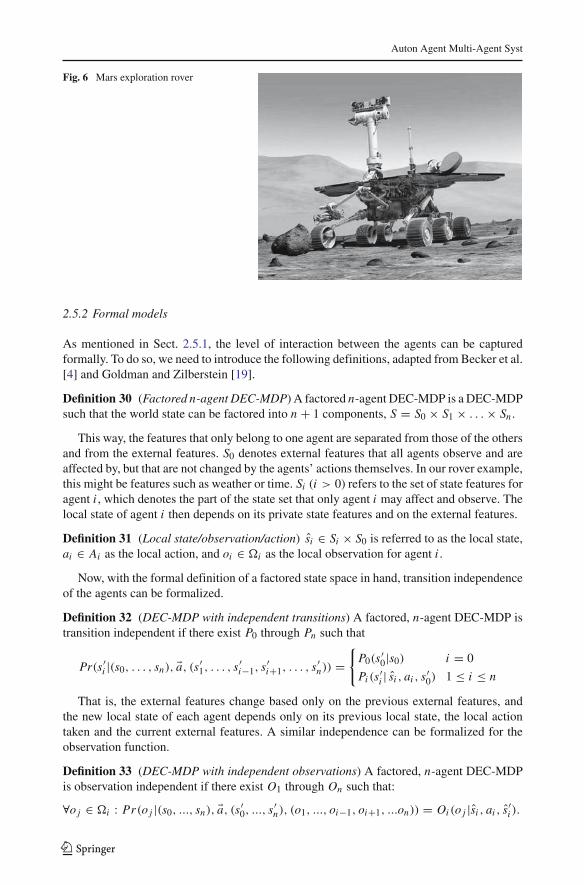
A real-world example of such a problem is that of controlling the operation of multipleplanetary exploration rovers, such as those used by NASA to explore the surface of Mars[50] (illustrated in Fig. 6). Each rover explores and collects information about its own par-ticular region. Periodically, the rovers can communicate with the ground control center butcontinuous communication is not possible. Some of the exploration sites overlap, and if tworovers collect information about these sites (e.g. take pictures) the reward is sub-additive.For other parts of the planet, the reward might be superadditive, for example if both roverswork together to build a 3D model of a certain area.
123
Auton Agent Multi-Agent Syst
Fig. 6 Mars exploration rover
2.5.2 Formal models
As mentioned in Sect. 2.5.1, the level of interaction between the agents can be capturedformally. To do so, we need to introduce the following definitions, adapted from Becker et al.[4] and Goldman and Zilberstein [19].
Definition 30 (Factored n-agent DEC-MDP) A factored n-agent DEC-MDP is a DEC-MDPsuch that the world state can be factored into n+ 1 components, S = S0 × S1 × . . .× Sn.
This way, the features that only belong to one agent are separated from those of the othersand from the external features. S0 denotes external features that all agents observe and areaffected by, but that are not changed by the agents’ actions themselves. In our rover example,this might be features such as weather or time. Si (i > 0) refers to the set of state features foragent i, which denotes the part of the state set that only agent i may affect and observe. Thelocal state of agent i then depends on its private state features and on the external features.
Definition 31 (Local state/observation/action) si ∈ Si × S0 is referred to as the local state,ai ∈ Ai as the local action, and oi ∈ �i as the local observation for agent i.
Now, with the formal definition of a factored state space in hand, transition independenceof the agents can be formalized.
Definition 32 (DEC-MDP with independent transitions) A factored, n-agent DEC-MDP istransition independent if there exist P0 through Pn such that
Pr(s′i |(s0, . . . , sn), �a, (s′1, . . . , s′i−1, s′i+1, . . . , s
′n)) =
{P0(s
′0|s0) i = 0
Pi(s′i | si , ai , s′0) 1 ≤ i ≤ n
That is, the external features change based only on the previous external features, andthe new local state of each agent depends only on its previous local state, the local actiontaken and the current external features. A similar independence can be formalized for theobservation function.
Definition 33 (DEC-MDP with independent observations) A factored, n-agent DEC-MDPis observation independent if there exist O1 through On such that:
∀oj ∈ �i : Pr(oj |(s0, ..., sn), �a, (s′0, ..., s′n), (o1, ..., oi−1, oi+1, ...on)) = Oi(oj |si , ai , s′i ).
123

Auton Agent Multi-Agent Syst
That is, the observation an agent receives depends only on that agent’s current and nextlocal state and current action.
Definition 34 (Local full observability) A factored, n-agent DEC-MDP is locally fully ob-servable if
∀oi ∃ si : Pr( si |oi) = 1.
That is, at each step, an agent’s observation fully determines its own local state. Notethat while observation independence and local full observability are related, it is possible forone to be true without the other. However, if both hold, both the set of observations and theobservation function in the definition of a factored n-agent DEC-MDP are redundant, andcan be omitted.
It is intuitive that if an agent’s transitions and observations in a DEC-MDP are independentfrom those of the other agents, the agent should be able to determine the local state givenits local observation. Goldman and Zilberstein [19] proved the following theorem whichformalizes this intuition:
Theorem 6 If a DEC-MDP has independent observations and transitions, then the DEC-MDP is locally fully observable.
Definition 35 (Reward independence) A factored, n-agent DEC-MDP is said to be rewardindependent if there exist f and R1 through Rn such that
R((s0, . . . , sn), �a, (s′0, . . . , s′n)) = f (R1( s1, a1, s′1), . . . , Rn( sn, an, s
′n))
and
Ri( si , ai , s′i ) ≤ Ri( si , a′i , s′′i ) ⇔
f (R1 . . . Ri( si , ai , s′i ) . . . Rn) ≤ f (R1 . . . Ri( si , a
′i , s′′i ) . . . Rn)
That is, the overall reward is composed of a function of the local reward functions, eachof which depends only on the local state and local action of one of the agents. Maximizingeach of the local reward functions individually is sufficient to maximize the overall rewardfunction.
Notice that a factored DEC-MDP with transition independence, observation independenceand reward independence decomposes into n independent local MDPs. Thus, the problembecomes P-complete and uninteresting from the perspective of decentralized control. How-ever, if just one of these independence relations is absent, the problem remains a non-trivialsubclass of DEC-MDPs.
The following section concentrates on the class of factored DEC-MDPs that are transitionand observation independent, but are not reward independent. Instead, the reward functionconsists of two different components. The first is a set of local reward functions that areindependent, just as in the case with multiple independent MDPs. The second component isan additional global reward (or penalty) that depends on the actions of all the agents, alongwith the global state. Thus, the overall model is not reward independent. It is formally definedby the joint reward structure, denoted ρ. This allows for defining interdependent rewards forcases where the whole system gets a reward after multiple agents have successfully com-pleted a task. The formal definition of a joint reward structure is beyond the scope of thispaper. We mention it here because it is necessary for the first theorem in the next section. SeeBecker et al. [4] for a formal definition and further details.
123

Auton Agent Multi-Agent Syst
2.5.3 Complexity results
The proofs for the theorems presented in this section can be found in Becker et al. [4] andGoldman and Zilberstein [19].
Theorem 7 Deciding a DEC-MDP with independent transitions and observations, and jointreward structure ρ is NP-complete.
At first sight, this model might seem very specialized and only applicable to a very smallset of problems. It turns out, however, that the class of problems addressed is quite gen-eral. Any reward dependence between multiple agents can be formalized using the jointreward structure ρ. There can still be different levels of independence in the reward function,affecting the efficiency of the representation of the joint reward structure.
The Mars rover example presented earlier falls into this class of problems. The rovershave independent transitions and observations. They mainly solve their tasks independently,but there may be tasks where they must work together to get a reward, e.g. by taking differentpictures of the same rock from different angles to be used in 3D model construction. A moredetailed example and an optimal algorithm (Coverage Set Algorithm) for this model canbe found in Becker et al. [4]. A significant improvement of the coverage set algorithm hasbeen presented by Petrik and Zilberstein [36]. A discussion of the complexity gap betweendecentralized problems that are NEXP-complete and problems that are NP-complete can befound in [44]. Beynier and Mouaddib [9] have also studied a restricted model of interactingMPDs in which the interaction is defined by temporal constraints. Additional restrictions onthe model give rise to another class of problems, which is even more specialized, and can besolved in polynomial time.
Definition 36 (Finite-horizon goal-oriented DEC-MDPs (GO-DEC-MDPs))3 A finite-horizon DEC-MDP is goal-oriented if the following conditions hold:
1. There exists a special subsetG of S of global goal states. At least one of the global goalstates g ∈ G is reachable by some joint policy.
2. The process ends at time T (the finite horizon of the problem).3. All actions in A incur a cost, C(ai) < 0. For simplicity, it is assumed that the cost of an
action depends only on the action. In general, this cost may also depend on the state.4. The global reward is R(s, �a, s′) = C(a1)+ . . .+ C(an).5. If at time T the system is in a state s ∈ G, there is an additional reward JR(s) ∈ � that
is awarded to the system for reaching a global goal state.
Definition 37 (Uniform cost) A goal-oriented DEC-MDP has uniform cost when the costsof all actions are the same.
Theorem 8 Deciding a goal-oriented DEC-MDP with independent transitions and obser-vations, with a single global goal state and with uniform cost is P-complete.
The following theorem helps explain the drop in complexity to NP and P respectively withthe last two models.
3 Adapted from Goldman and Zilberstein [19].
123
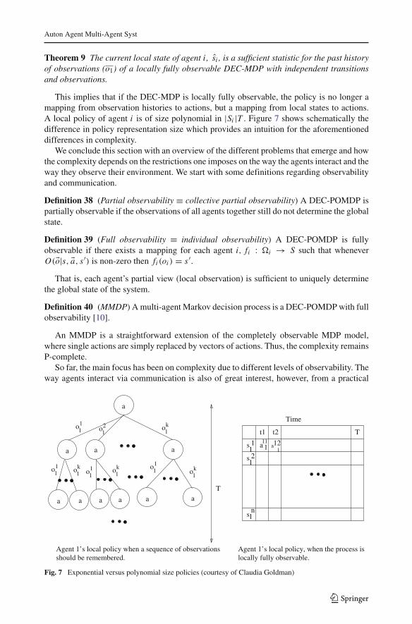
Auton Agent Multi-Agent Syst
Theorem 9 The current local state of agent i, si , is a sufficient statistic for the past historyof observations (o1) of a locally fully observable DEC-MDP with independent transitionsand observations.
This implies that if the DEC-MDP is locally fully observable, the policy is no longer amapping from observation histories to actions, but a mapping from local states to actions.A local policy of agent i is of size polynomial in |Si |T . Figure 7 shows schematically thedifference in policy representation size which provides an intuition for the aforementioneddifferences in complexity.
We conclude this section with an overview of the different problems that emerge and howthe complexity depends on the restrictions one imposes on the way the agents interact and theway they observe their environment. We start with some definitions regarding observabilityand communication.
Definition 38 (Partial observability ≡ collective partial observability) A DEC-POMDP ispartially observable if the observations of all agents together still do not determine the globalstate.
Definition 39 (Full observability ≡ individual observability) A DEC-POMDP is fullyobservable if there exists a mapping for each agent i, fi : �i → S such that wheneverO(�o|s, �a, s′) is non-zero then fi(oi) = s′.
That is, each agent’s partial view (local observation) is sufficient to uniquely determinethe global state of the system.
Definition 40 (MMDP) A multi-agent Markov decision process is a DEC-POMDP with fullobservability [10].
An MMDP is a straightforward extension of the completely observable MDP model,where single actions are simply replaced by vectors of actions. Thus, the complexity remainsP-complete.
So far, the main focus has been on complexity due to different levels of observability. Theway agents interact via communication is also of great interest, however, from a practical
o11
o1
o1
o1
o11
o1o
1o
1o11
2 k
k 1 k k
T
a
a a
a a a aa a
a
Agent 1’s local policy, when the process islocally fully observable.
Agent 1’s local policy when a sequence of observations should be remembered.
Time
t1 t2 T
s 11
s12
s1n
a 111
a1
12
Fig. 7 Exponential versus polynomial size policies (courtesy of Claudia Goldman)
123
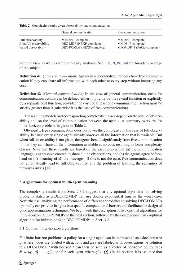
Auton Agent Multi-Agent Syst
Table 2 Complexity results given observability and communication
General communication Free communication
Full observability MMDP (P-complete) MMDP (P-complete)Joint full observability DEC-MDP (NEXP-complete) MMDP (P-complete)Partial observability DEC-POMDP (NEXP-complete) MPOMDP (PSPACE-complete)
point of view as well as for complexity analyses. See [18,19,39] and for broader coverageof the subject.
Definition 41 (Free communication) Agents in a decentralized process have free communi-cation if they can share all information with each other at every step without incurring anycost.
Definition 42 (General communication) In the case of general communication, costs forcommunication actions can be defined either implicitly by the reward function or explicitlyby a separate cost function, provided the cost for at least one communication action must bestrictly greater than 0 (otherwise it is the case of free communication).
The resulting models and corresponding complexity classes depend on the level of observ-ability and on the level of communication between the agents. A summary overview forfinite-horizon problems is given in Table 2.
Obviously, free communication does not lower the complexity in the case of full observ-ability, because every single agent already observes all the information that is available. Butwhen full observability is not given, the agents benefit significantly from free communicationin that they can share all the information available at no cost, resulting in lower complexityclasses. Note that these results are based on the assumptions that (a) the communicationlanguage is expressive enough to share all the observations, and (b) the agents agree before-hand on the meaning of all the messages. If this is not the case, free communication doesnot automatically lead to full observability, and the problem of learning the semantics ofmessages arises [17].
3 Algorithms for optimal multi-agent planning
The complexity results from Sect. 2.3.2 suggest that any optimal algorithm for solvingproblems stated as a DEC-POMDP will use double exponential time in the worst case.Nevertheless, analyzing the performance of different approaches to solving DEC-POMDPsoptimally can provide insights into specific computational barriers and facilitate the design ofgood approximation techniques. We begin with the description of two optimal algorithms forfinite-horizon DEC-POMDPs in the next section, followed by the description of an ε-optimalalgorithm for infinite-horizon DEC-POMDPs in Sect. 3.2.
3.1 Optimal finite-horizon algorithms
For finite-horizon problems, a policy for a single agent can be represented as a decision treeq, where nodes are labeled with actions and arcs are labeled with observations. A solutionto a DEC-POMDP with horizon t can then be seen as a vector of horizon-t policy treesδt = (qt1, qt2, . . . , qtn), one for each agent, where qti ∈ Qt
i . (In this section, it is assumed that
123
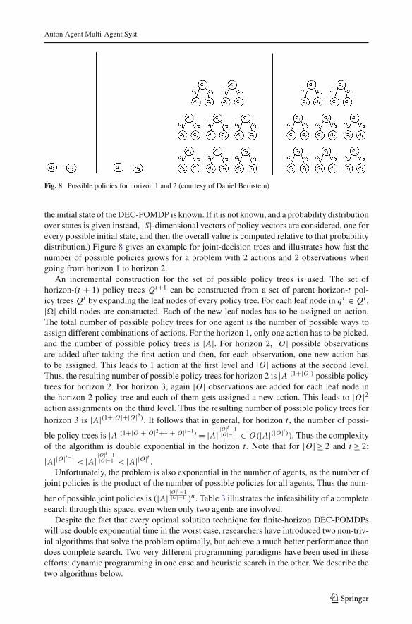
Auton Agent Multi-Agent Syst
Fig. 8 Possible policies for horizon 1 and 2 (courtesy of Daniel Bernstein)
the initial state of the DEC-POMDP is known. If it is not known, and a probability distributionover states is given instead, |S|-dimensional vectors of policy vectors are considered, one forevery possible initial state, and then the overall value is computed relative to that probabilitydistribution.) Figure 8 gives an example for joint-decision trees and illustrates how fast thenumber of possible policies grows for a problem with 2 actions and 2 observations whengoing from horizon 1 to horizon 2.
An incremental construction for the set of possible policy trees is used. The set ofhorizon-(t + 1) policy trees Qt+1 can be constructed from a set of parent horizon-t pol-icy treesQt by expanding the leaf nodes of every policy tree. For each leaf node in qt ∈ Qt ,|�| child nodes are constructed. Each of the new leaf nodes has to be assigned an action.The total number of possible policy trees for one agent is the number of possible ways toassign different combinations of actions. For the horizon 1, only one action has to be picked,and the number of possible policy trees is |A|. For horizon 2, |O| possible observationsare added after taking the first action and then, for each observation, one new action hasto be assigned. This leads to 1 action at the first level and |O| actions at the second level.Thus, the resulting number of possible policy trees for horizon 2 is |A|(1+|O|) possible policytrees for horizon 2. For horizon 3, again |O| observations are added for each leaf node inthe horizon-2 policy tree and each of them gets assigned a new action. This leads to |O|2action assignments on the third level. Thus the resulting number of possible policy trees forhorizon 3 is |A|(1+|O|+|O|2). It follows that in general, for horizon t , the number of possi-
ble policy trees is |A|(1+|O|+|O|2+···+|O|t−1)= |A| |O|t−1
|O|−1 ∈ O(|A|(|O|t )). Thus the complexityof the algorithm is double exponential in the horizon t . Note that for |O| ≥ 2 and t ≥ 2:
|A||O|t−1< |A| |O|
t−1|O|−1 < |A||O|t .
Unfortunately, the problem is also exponential in the number of agents, as the number ofjoint policies is the product of the number of possible policies for all agents. Thus the num-
ber of possible joint policies is (|A| |O|t−1
|O|−1 )n. Table 3 illustrates the infeasibility of a completesearch through this space, even when only two agents are involved.
Despite the fact that every optimal solution technique for finite-horizon DEC-POMDPswill use double exponential time in the worst case, researchers have introduced two non-triv-ial algorithms that solve the problem optimally, but achieve a much better performance thandoes complete search. Two very different programming paradigms have been used in theseefforts: dynamic programming in one case and heuristic search in the other. We describe thetwo algorithms below.
123

Auton Agent Multi-Agent Syst
Table 3 Possible policies with 2actions and 2 observations
Horizon Policies for one agent Joint-policies for 2 agents
1 2 42 8 643 128 16,3844 32,768 1,073,741,8245 2,147,483,648 4.6 · 1018
3.1.1 Dynamic programming for DEC-POMDPs and POSGs
The first non-trivial algorithm for finding optimal solutions in DEC-POMDPs was presentedby Hansen et al. [22]. This algorithm finds sets of policies for partially observable stochasticgames (POSGs), which are a special kind of extensive games with imperfect information[30]. POSGs only differ from DEC-POMDPs in that they allow for one private reward func-tion per agent, thus allowing non-cooperative behavior. When applied to DEC-POMDPs,this algorithm finds an optimal joint policy. The algorithm generalizes two previously devel-oped techniques: dynamic programming for POMDPs [21] and elimination of dominatedstrategies in normal form games.
The main idea of dynamic programming for POMDPs is to incrementally search throughthe space of possible policies, pruning dominated policies as early as possible in the con-struction process to avoid the full exhaustive backup. Therefore, the POMDP first has to beconverted into a completely observable MDP with a state set B = �S that consists of allpossible beliefs about the current state. Furthermore, the algorithm exploits the fact that thevalue function for a POMDP can be represented exactly by a finite set of |S|-dimensionalvalue vectors, denoted V = {v1, v2, . . . , vk}, where
V (b) = max1≤j≤k
∑s∈S
b(s)vj (s)
Every value vector vj corresponds to a complete conditional plan, i.e. a policy tree. Thedynamic programming (DP) operator exploits this fact when pruning dominated policy tress.
Definition 43 (Dominated policy trees) A policy tree qj ∈ Qt with corresponding valuevector vj ∈ V t is considered dominated if for all b ∈ B there exists a vk ∈ V t\vj such thatb · vk ≥ b · vj .
In every iteration of dynamic programming, the DP operator is first given a setQt of depth-t policy tress and a corresponding set V t of values vectors. The setsQt+1 and V t+1 are thencreated by an exhaustive backup. This operation generates every possible depth-t + 1 policytree that makes a transition, after an action and observation, to the root node of some depth-tpolicy tree. In the next step, all dominated policy trees are eliminated from the set Qt+1
(the test for dominance is performed using linear programming). This can be done becausea decision maker that is maximizing expected value will never follow a dominated policyand thus the DP operator does not decrease the value of any belief state. After the exhaustivebackup and before the pruning step, the size of the set of policy trees is |Qt+1| = |A||Qt ||O|.
Unfortunately, the DP operator for POMDPs cannot be generalized in a straightforwardway, because there is no notion of a belief state in a DEC-POMDP. Only beliefs about thestrategies of other agents can be formulated, similar to some ideas concerning normal formgames (cf. [22]). A generalized belief state has to be defined, synthesizing a belief overpossible states and a distribution over the possible policies of the other agents. Let Qt
−i
123

Auton Agent Multi-Agent Syst
denote the set of horizon-t policy trees for all agents except i. For each agent i, a belieffor a horizon-t DEC-POMDP is now defined as a distribution over S × Qt
−i . The set ofvalue vectors for agent i is thus of dimension |S × Qt
−i |. This set of value vectors is thebasis for elimination of very weakly dominated policies in the multi-agent case, just as forPOMDPs.
Definition 44 (Very Weakly Dominated Policy Trees) A policy tree qj ∈ Qti with corre-
sponding value vector vj ∈ V ti is very weakly dominated if
∀b ∈ �(S ×Qt−i ), ∃vk ∈ V ti \ vj such that b · vk ≥ b · vj
Now, multiple agents are considered instead of one single agent. When agent i eliminatesits dominated policies this can affect the best policy of agent j . Thus, elimination of policieshas to include alternation between agents until no agent can eliminate another policy. Thisprocedure is called iterated elimination of dominated strategies. With the generalized beliefstate, given a horizon-t POSG it would now be possible to generate all horizon-t policy treesand the corresponding value vectors. Then, iterated elimination of very weakly dominatedstrategies could be applied to solve the problem and find the optimal policy. Unfortunately,as pointed out in the beginning, generating all possible horizon-t policy trees is infeasibledue to the double exponential dependence on the time horizon t .
The DP operator for POMDPs can be generalized to the multi-agent case by interleav-ing exhaustive backups with pruning of dominated policies. In the first step of an iteration,the multi-agent DP operator is given Qt
i and generates Qt+1i . In the second step, all very
weakly dominated policies are pruned. As in the single agent case, this does not reduce theoverall value because for every policy tree that has a very weakly dominated subtree thereis a probability distribution over other policy trees that leads to a stochastic policy yieldingthe same or higher value. Thus, applying dynamic programming for POSGs eventually leadsto a set of horizon-t policy tress including the optimal solution. For the special case of aDEC-POMDP, the algorithm preserves at least one optimal policy. When the multi-agent DPoperator reaches horizon t , a policy can be chosen, by extracting the highest-valued policytree according to the initial state distribution.
Of course, the algorithm is still doubly exponential in the time horizon t in the worst case.Any improvement over brute force search depends on the amount of possible pruning, whichdepends on the particular problem. The algorithm has been tested on the multi-access broad-cast channel problem, described in Sect. 1.1.1. Table 4 illustrates the possible improvementsin practice. For the horizon 4, the dynamic programming algorithm produces less than 1% ofthe number of policy trees produced by the brute force algorithm. Note that the brute forcealgorithm could not actually complete iteration 4.
Unfortunately, the dynamic programming algorithm runs out of memory after the 4th iter-ation due to the rapid growth in the number of policies trees. Even with pruning, an exhaustivebackup going from horizon 4 to horizon 5 would need to produce 2 · 3004, or more than 16
Table 4 Performancecomparison: number of policiesfor each agent
Horizon Brute force search Dynamic programmingalgorithm
1 (2, 2) (2, 2)2 (8, 8) (6, 6)3 (128, 128) (20, 20)4 (32,768, 32,768) (300, 300)
123

Auton Agent Multi-Agent Syst
billion S-dimensional vectors of policy trees, before even beginning the process of pruning.This explains why the algorithm runs out of memory long before running out of time.
3.1.2 MAA∗: a heuristic search algorithm for DEC-POMDPs
In 2005, Szer et al. [48] presented an approach orthogonal to dynamic programming forDEC-POMDPs, based on heuristic search. As we discuss in Sect. 3.1.3, the method has bothadvantages and disadvantages over the dynamic programming algorithm. The algorithm isbased on the widely used A∗ algorithm, and performs best-first search in the space of possiblejoint policies.
The algorithm uses the same representation for joint policies as presented earlier in thissection: qti is a depth-t policy tree for agent i and δt = (qt1, . . . , qtn) is a policy vector of trees.Furthermore, let V (s0, δ) denote the expected value of executing policy vector δ from states0. Finding the optimal joint policy is thus identical to finding δ∗T = argmaxδT V (s0, δ). Asin brute force search, the algorithm searches in the space of policy vectors, where nodes atlevel t of the search tree correspond to partial solutions of the problem, namely policy vec-tors of horizon t . But unlike complete search, not all nodes at every level are fully expanded.Instead, a heuristic function is used to evaluate the leaf nodes of the search tree. The nodewith the highest heuristic estimate is expanded in each step. Figure 9 shows a section of sucha multi-agent search tree.
To compute the heuristic estimate of a search node, the evaluation function is decomposedinto two parts: an exact evaluation of the partial solution (the policy vector up to the currentlevel), and a heuristic estimate of the remaining part, the so called completion.
Definition 45 (Completion of a policy vector) A completion �T−t of an arbitrary depth-tpolicy vector is a set of depth-(T − t) policy trees that can be attached at the leaf nodes of apolicy vector δt such that {δt ,�T−t } constitutes a complete policy vector of depth T .
Now, the value of any depth-T policy vector also decomposes into two parts:
V (s0, {δt ,�T−t }) = V (s0, δt )+ V (�T−t |s0, δt )Fig. 9 A section of themulti-agent A∗ search tree,showing a horizon 2 policy vectorwith one of its expanded horizon3 child nodes (courtesy of DanielSzer)
a a a
a b
a
b
a a b a
a b
a
3q1
3q 2
a b
b
q12 q2
2
b
ao1 o1 o2o2
o1 o1o2 o2
o2o2 o1o1o2o2 o1o1
... ...
3δ =
2δ =
a
2 agents,
2 actions (a and b)2 observations (o and o ),1 2
123

Auton Agent Multi-Agent Syst
Obviously, the value of the completion depends on the state distribution that is reachedafter executing policy vector δt in state s0. Instead of computing its value exactly, we willestimate it efficiently via heuristic function H . We thus define the value estimate of state s0and policy δt as:
F(s0, δt ) = V (s0, δt )+HT−t (s0, δt )
For the heuristic search to be optimal and complete, the function H must be admissible, i.e.an overestimate of the exact value of the optimal completion of policy vector δt :
∀�T−t : HT−t (s0, δt ) ≥ V (�T−t |s0, δt )It is crucial for the algorithm to have an admissible heuristic function that is efficiently com-putable and as close as possible to the true value of the state (to maximize the amount ofpruning). To describe the admissible heuristics used by the algorithm, we use the followingnotation:
• P(s|s0, δ) is the probability of being in state s after executing the policy tree vector δfrom s0.• ht (s) is an optimistic value function heuristic for the expected sum of rewards when
executing the best vector of depth t policy trees from state s, i.e. ht (s) ≥ V ∗t (s).Now the following class of heuristic functions can be defined:
HT−t (s0, δt ) =∑s∈S
P (s|s0, δt )hT−t (s)
Any function in this class simulates the situation where the real underlying state is revealedto the agents at time t after execution of policy vector δt . Intuitively, any such heuristic His admissible, if h is admissible (for a detailed proof see [48]). Fortunately, when computingthe heuristic estimate for the value of a policy vector of depth t and state s0, the doubleexponential number of possible completions does not have to be computed. Instead, h onlyhas to be computed for every possible state, thus |S| times. This leads to major savings. Szeret al. [48] have presented three different heuristics for the MAA∗ algorithm:
1. The MDP heuristic: A strong simplification is to consider the underlying centralizedMDP with remaining finite horizon T − t : hT−t (s) = VMDP
T−t (s). Because solving anMDP only takes polynomial time, this is an efficient way to compute the heuristic, butleads to a huge overestimate.
2. The POMDP heuristic: Considering the underlying POMDP leads to a tighter value func-tion heuristic and thus allows more pruning. Unfortunately, solving POMDPs is PSPACE-complete, thus this heuristic is also more complex to compute.
3. Recursive MAA∗: Among the heuristics that simulate revealing the underlying systemstate, the tightest heuristic possible is given by the optimal value itself: ht (s) = V ∗t (s).This value can be efficiently computed by applying MAA∗ recursively: hT−t (s) =MAA∗T−t (s). Calling MAA∗T invokes |S| subcalls of MAA∗T−1. Note that this proce-dure is exponential in t as compared to a complete search, which is double exponentialin t .
Obviously, there is a tradeoff between the tightness of the heuristic and the complexityof computing it. Due to the double exponential growth of the search tree, a tighter yet morecomplex heuristic has proven to be best in experimental results. So far, the MAA∗ algorithmusing the recursive heuristic function is the only algorithm found to be able to solve themulti-agent tiger problem (as presented in Sect. 1.1.2) with 2 states, 2 agents, 3 actions and 2
123

Auton Agent Multi-Agent Syst
observations up to horizon 4. MAA∗ runs out of time when computing horizon 5. To improvescalability, approximation techniques such as those presented in Sect. 4 must be used.
3.1.3 Limitations of MAA∗
Szer et al. [48] note that due to the double exponential dependence on the time horizon T ,evaluating the search tree until depth T −1 is “easy,” i.e. almost all of the computationaleffort is dedicated to the last level of the policy tree. Completely expanding a node at levelT −1 and creating all its level T children takes a lot of time. However, if the value estimateof one of these children is as high as the value estimate of its parent (which is called a tie),the other children do not have to be considered. Thus, in the implementation of MAA∗, theauthors have used incremental node expansion. This means that only one child assignmentof actions is constructed in each iteration and then the value of this child is computed. Aslong as some children need to be generated, the parent remains in an open list. The authorsargue that this might lead to considerable savings in both memory and runtime.
An obstacle is that incremental node expansion only saves time when the value estimate of anode actually coincides with the value estimate of the best child:FT (s0, δt−1) = FT (s0, δ∗t ).Even if this were the case, however, many children would have to be generated before thebest is picked. So far, it is not known if there is a fast way to find the best child. Heuristicsfor finding the best child might exist, but good ones are likely to be problem-dependent. Infact, for this procedure to be effective, revealing the true system state to all agents at mustlead to the same value estimate as before, regardless of the state. This seems very unlikely indecentralized problems. For example, consider the multi-agent tiger problem, where reveal-ing the true system state would actually have a huge impact on the agent’s expected value. Ifthe true system state is revealed to the agents, the agents know the location of the tiger andthus they can open the door that leads to treasure with probability 1. In most problems, theseties will not occur and thus incremental node expansion will not be very effective. Obviously,heuristics that do not reveal the underlying system state do not suffer from this problem. Butso far, no such heuristic has been proposed.
The low likelihood of ties is a significant drawback, limiting the applicability of MAA∗.When at least one node is expanded at level T −1 with no ties, all of its children must begenerated to find the optimal solution for horizon T . Completely expanding just one of thelast search nodes, in going from level T−1 to level T , creates (|A|(|�|T−1))n new child nodes.Thus, in general, the MAA∗ algorithm can at best solve problems whose horizon is only 1greater than those that can already be solved by naive brute force search. This conclusion isillustrated by the empirical results shown in Table 5.
As shown, the MAA∗ algorithm can solve the multi-agent tiger problem with horizon 4,whereas brute force search can only solve horizon 3. As already explained, however, MAA∗evaluates more nodes for the horizon 4 problem than the brute force algorithm does for thehorizon 3 problem. The same would be true in comparing horizon 4 with horizon 5. This
Table 5 Performancecomparison: evaluated policypairs
Horizon Brute force search Recursive MAA∗
1 9 92 729 1713 4,782,969 26,4154 2.06 · 1014 344,400,1835 3.82 · 1029 >2.06 · 1014
123

Auton Agent Multi-Agent Syst
means that MAA∗ would have to evaluate more than 2.06 · 1014 nodes to solve the horizon5 problem, independent of the heuristic used.
Another recent research direction has examined weighted heuristics, i.e. f (s) = g(s)+w ·h(s). If the weightw is greater than 1, the heuristic becomes non-admissible and the search isno longer optimal, but can find suboptimal solutions faster, as it goes deep into the search treemore quickly. The idea is that after suboptimal solutions have been found, large chunks of thesearch tree can be pruned, thus reducing significantly the size of the open list. If the open listbecomes empty, the last solution generated is optimal. Because keeping a large open list inmemory has an impact on the entire search process, this can lead to a considerable speedup.Unfortunately, with double exponential dependence on the time horizon, this approach doesnot yield considerable savings because at least one node at level T−1 must be fully expanded(if no tie occurs). Again, as this is already as much work as a brute force search would dofor a problem with horizon T −1, the problem remains almost as hard to solve.
Note that the MAA∗ algorithm runs out of time before it runs out of memory, in contrastto the dynamic programming algorithm, which runs out of memory long before it runs outof time. Furthermore, the MAA∗ algorithm makes use of the common reward function of theagents but does not take into account at all that it is dealing with a DEC-POMDP problem.On the other hand, the dynamic programming algorithm does exploit the fact that it is dealingwith a DEC-POMDP by pruning dominated strategies. A more promising approach seemsto be combining heuristic search with dynamic programming, yielding a better and moresophisticated algorithm for finding approximate solutions for finite-horizon DEC-POMDPs.Such an approach is presented in Sect. 4.2.
3.2 An ε-optimal infinite-horizon algorithm
The solution techniques presented in the previous section do not work for infinite-horizonDEC-POMDPS because we cannot build infinitely long policy tress which would require aninfinite amount of memory. Thus, a different representation for the policies has to be used thatonly uses a finite amount of memory. Note that while we no longer have a finite time horizonT , all definitions of infinite-horizon DEC-POMDPs need a discount factor γ ∈ [0, 1).
Because infinite-horizon DEC-POMDPs are undecidable, one cannot hope for a trulyoptimal algorithm for this class. In 2005, Bernstein [5] presented a policy iteration algorithmfor infinite-horizon DEC-POMDPs that converges to ε-optimal solutions in the limit. Weoutline this approach below.
Definition 46 (Local finite-state controller) A local finite-state controller for agent i is atuple 〈Qi,ψi, ηi〉, where:
• Qi is a finite set of controller nodes.• ψi : Qi → �Ai is a stochastic action selection function.• ηi : Qi × Ai ×Oi → �Qi is a stochastic transition function.
Definition 47 (Independent joint controller) A set of local finite-state controllers, one foreach agent, determines the conditional distribution P(�a, �q ′|�q, �o), referred to as an indepen-dent joint controller.
This way of representing a joint policy is called an independent joint controller becausethere is no direct correlation between the agents. Each agent’s local policy depends only onits own memory state. As Bernstein has demonstrated, however, some form of correlationbetween the agents might be beneficial.
123

Auton Agent Multi-Agent Syst
Fig. 10 A DEC-POMDP whoseoptimal memory-bounded jointpolicy requires correlation(courtesy of Daniel Bernstein)
3.2.1 The utility of correlation
Figure 10 shows a DEC-POMDP that illustrates the importance of correlation. In this exam-ple, there are two states, two agents, two actions per agent (A and B) and one observation.Because there is just one observation, the agents cannot distinguish between the two differentstates. Below, two memoryless policies for this problem are compared:
• Because the agents do not know the state they are in, each deterministic policy will bearbitrarily bad in the long run. If both agents can randomize independently, the best theycould do is choose either action A or B according to a uniform distribution in each step.With an expected reward of−R/2 per time step this yields an expected long-term rewardof −R/2(1− γ ).• If the agents can correlate their policies using a common source of randomness, the best
policy would be to execute the joint action AA with probability 1/2 and BB with proba-bility 1/2. This leads to an expected long term reward of 0. Thus, the difference betweencorrelated and uncorrelated strategies can be made arbitrarily large by increasing R.
This example shows the need for correlation when representing joint policies with boundedmemory. The importance of stochastic correlation was also proposed by Peshkin et al. [35].They presented an algorithm that uses gradient descent in policy space to find locally opti-mal solutions for multi-agent problems. While that technique was focused on multi-agentlearning rather than planning, it has provided important insights regarding the usefulness ofcorrelation.
3.2.2 Correlated joint controllers
To allow for correlation, Bernstein et al. [7] introduce a correlation device in the form of anadditional finite-state machine. The correlation device is some random process that does nothave any access to the observations available to the agents. All agents have access to extrasignals from the device in each time step, but cannot exchange information via the correlationdevice.
Definition 48 (Correlation device) A correlation device is a tuple 〈C,ψ〉, where:
• C is a finite set of states.• ψ : C → �C is a state transition function.
At each time step, the device makes a transition and all agents observe the new state.
Now, the definition of a local controller has to be extended to consider the correlationdevice. The action taken by each agent and the controller state transitions become dependenton the input signal c. Thus, the local controller for agent i is a conditional distribution of theform P(ai, q
′i |c, qi, oi).
123

Auton Agent Multi-Agent Syst
Definition 49 (Correlated joint controller) A correlation device together with the local con-trollers for each agent form a joint conditional distribution P(c′, �a, �q ′|c, �q, �o), called a cor-related joint controller.
The value of a correlated joint controller can then be computed by solving a set of linearequations, one for each s ∈ S, �q ∈ �Q, and c ∈ C:
V (s, �q, c) =∑�aP (�a|c, �q)
⎡⎣R(s, �a)
+ γ∑
s′,�o,�q ′,c′P(s′, �o|s, �a)P (�q ′|c, �q, �a, �o)P (c′|c)V (s′, �q ′, c′)
⎤⎦
3.2.3 Policy iteration for infinite-horizon DEC-POMDPs
As there are infinitely many possible observation sequences for the infinite-horizon case, anyfinite set of states of a correlated joint controller may be insufficient to produce an optimalsolution. To guarantee ε-convergence, it is necessary to increase the number of controllerstates successively. This can be accomplished using an exhaustive backup, which we havealready introduced for the finite-horizon DP algorithm. Here, instead of growing policy treesin a top-down manner, we iteratively grow the local controllers, for all agents at once, leavingthe correlation device unchanged.
To formalize this process, let Qti denote the set of controller nodes for agent i after iter-
ation t . For each possible one-step policy, a new controller node is added. Thus, for eachagent i, |Ai ||Qi ||�i | nodes are added to the controller. In the finite-horizon algorithm, theexhaustive backup was followed by a pruning step, eliminating dominated policy trees. Here,an analogous procedure can be used [5].
Definition 50 (Value-preserving transformation) Given two correlated joint controllers Cand D with node sets �Q and �R respectively, we say that changing controller C to D is avalue-preserving transformation if there exist mappings fi : Qi → �Ri for each agent iand fc : Qc → �Rc such that:
V (s, �q) ≤∑�rP (�r|q)V (s, �r) ∀s ∈ S, �q ∈ �Q
The goal of a value-preserving transformation is to reduce the size of a controller withoutdecreasing its value, or to improve the value without changing the size. In general, reducingthe size of the controller is necessary between exhaustive backup steps because those stepsincrease the size of the controller in a double exponential manner. Bernstein [5] formulatedseveral such transformations that can be implemented efficiently using linear programming.
Similar to the finite-horizon case, exhaustive backups are interleaved with value-preservingtransformations. However, for the infinite-horizon case we need an explicit stopping crite-rion. Because there is no Bellman residual for testing convergence as in single agent MDPs,it is necessary to use the discount factor γ and the number of iterations to define a simplerε-convergence test. Let |Rmax| denote the largest absolute value of a one-step reward in theDEC-POMDP. Then the algorithm terminates after iteration t if γ t+1 · |Rmax|/(1− γ ) ≤ ε.Intuitively, the algorithm exploits the fact that due to discounting, at some point the futurerewards collected are negligible. The complete procedure is sketched in Algorithm 1.
123

Auton Agent Multi-Agent Syst
Algorithm 1: Policy iteration for infinite-horizon DEC-POMDPsinput : DEC-POMDP problem, random correlated joint controller, convergence parameter εoutput: A correlated joint controller that is ε-optimal for all statesbegin
t ← 0while γ t+1 · |Rmax |/(1− γ ) > ε do
t ← t + 1Evaluate the correlated joint controller by solving a system of linear equationsPerform an exhaustive backup to add nodes to the local controllersPerform value-preserving transformations on the controller
return correlated joint controllerend
The convergence of the algorithm is characterized by the following theorem [5].
Theorem 10 For any ε, policy iteration returns a correlated joint controller that is ε-optimalfor all initial states in a finite number of iterations.
As with optimal algorithms for finite-horizon DEC-POMDPs, the policy iteration algo-rithm for infinite-horizon problems is mainly of theoretical significance. In practice, thevalue-preserving transformations cannot reduce the size of the controllers sufficiently tocontinue executing the algorithm until the convergence criterion is met. The algorithm runsout of memory after a few iterations even for small problems. However, several approximatetechniques for infinite-horizon DEC-POMDPs have been developed that restrict the size ofeach controller and optimize value with a bounded amount of memory. We present two suchapproaches in Sect. 5.
4 Approximate algorithms for finite-horizon problems
Due to the high computational complexity of DEC-POMDPs, developing approximationtechniques rather than exact algorithms seems more fruitful in practice. Unfortunately, aswas shown by Rabinovich et al. [40], even ε-optimal history-dependent joint policies arestill NEXP-hard to find in both DEC-POMDPs and DEC-MDPs. Thus, when looking forapproximate solutions that are computationally tractable, the global value has to be sacri-ficed to lower the complexity and to handle larger problems. At this point, a small ambiguityin the term “approximation” must be discussed. In the field of theoretical computer science,an “approximation algorithm” generally denotes an algorithm that provides some provableguarantees on the solution quality. These performance guarantees can for example be relativeguarantees (the approximation will be no worse than a factor of c of the optimal solution) orabsolute guarantees (the approximation will be within ε of the optimal solution). Approxi-mation algorithms are normally used to find solutions for NP-hard optimization problems,and a polynomial running time is generally required.
In the AI community, the term “approximation” is used in a less strict sense. In this paper,we differentiate between optimal algorithms (that always find the optimal solution), ε-optimalalgorithms (that guarantee a performance within ε of the optimal solution) and approximatealgorithms (i.e. heuristics that have no performance guarantees at all). In this section we pres-ent approximate algorithms that do not guarantee any bounds on the solution quality withregard to the optimal solution. Furthermore, some of them do not even guarantee a polynomialworst case running time, which is still acceptable in light of the NEXP-completeness result.Due to these missing guarantees, however, it is difficult to compare the different approxima-tion techniques. A few benchmark problems have been established and can be used for initial
123

Auton Agent Multi-Agent Syst
comparison of running time and solution value. In the long run, a whole suite of problems hasto be established such that good comparable benchmark tests can be performed. Comparablecompetitions already exist for the field of centralized deterministic planning algorithms butare still to be established for the field of decentralized planning under uncertainty. In Sect. 7we will summarize the different approaches presented in this section and try a comparisonwhere possible.
4.1 Overview of recent approximation techniques
One approach for finding approximate algorithms for decentralized problems is to generalizeexisting approximate algorithms for POMDPs. Unfortunately, most of those algorithms usea compact representation of the belief state space. So far, no such compact representation hasbeen found for DEC-POMDPs, mostly because an agent’s belief is not only dependent onits own local view of the problem, but also on the other agents. Thus, generalizing existingalgorithms for POMDPs is not straightforward.
In 2003, Nair et al. [26] presented a class of algorithms, called “Joint Equilibrium-Based Search for Policies” (JESP), that do not search for the globally optimal solution of aDEC-POMDP, but instead aim for local optimality. The best algorithm, DP-JESP, incorpo-rates three different ideas. First, the policy of each agent is modified while keeping the policiesof the others fixed (a similar idea is presented in Sect. 5.1). Second, dynamic programmingis used to iteratively construct policies. This is analogous to the idea presented in Sect. 3.1.1.Third, and most notably, only reachable belief states of the DEC-POMDP are considered forpolicy construction. This leads to a significant improvement, because there is only an expo-nential number of different belief states for one agent as opposed to the double exponentialnumber of possible joint policies. The algorithm is able to solve small problems such as themulti-agent tiger problem up to horizon 7. Thus, it is an improvement over the exact algorithms(which work only up to horizon 4), although it does not scale well for larger problem sizes.
Emery-Montemerlo et al. [15] take a game-theoretic approach, modeling the problem asa POSG with common payoffs. In contrast to the other algorithms discussed in this paper,this is an online algorithm which interleaves planning and execution. The POSG is approx-imated as a series of smaller Bayesian games. In each of these simple games, the agentsonly have to decide on the next action to take based on a one-step lookahead. The futurereward after taking one action is estimated using heuristics such as QMDP , which turns theremaining problem into a fully-observable problem. Similar to the dynamic programmingalgorithm proposed by Nair et al. [26], the algorithm solves the resulting Bayesian gamesusing an alternating-maximization algorithm, where the best response strategy of one agentis computed while the strategies of the other agents are held fixed. In each iteration, beforethe agents select an action they match their history of local observations and actions withone of the types in their local type space found by solving the Bayesian game. To limit mem-ory requirements for remembering the history of actions and observations, low-probabilityhistories are pruned. These simplifying assumptions (1. treating the problem as a series ofsmaller games with one-step lookahead, 2. computing future rewards using a heuristic, and 3.using the alternating-maximization algorithm) lead to some obvious value loss. However, thealgorithm is able to solve substantially larger problems compared to Nair et al. [26], largelydue to the fact that planning and execution are interleaved in an intelligent way.
Within the scope of this study, it is not possible to cover all recently developed approx-imate algorithms for DEC-POMDPs in detail. Instead, we limit ourselves to the details ofthe Improved Memory-Bounded Dynamic Programming (IMBDP) algorithm, as it has out-performed all recently proposed approximation methods. IMBDP can solve problems with
123

Auton Agent Multi-Agent Syst
horizons that are multiple orders of magnitude larger than what was previously possible,while achieving the same or better solution value.
4.2 Improved memory-bounded dynamic programming (IMBDP)
In 2007, we introduced the original MBDP [42] as well as the improved MBDP algorithm[43]. This section is based on these two papers, summarizing the main ideas.
The method is based on the dynamic programming algorithm, presented in Sect. 3.1.1.As we have seen, even if pruning techniques are used (elimination of dominated policies) inthe bottom-up construction of the policy trees, the number of trees still grows too quicklyand the algorithm runs out of memory. An analysis of the construction process reveals thatmost policies kept in memory are useless because a policy tree can only be eliminated if itis dominated for every belief state. For many DEC-POMDPs, however, only a small subsetof the belief space is actually reachable. Furthermore, a policy tree can only be eliminatedif it is dominated for every possible belief over the other agents’ policies. Obviously, duringthe construction process, these other agents also maintain a large set of policy trees that willeventually prove to be useless.
Unfortunately, with a bottom-up approach, these drawbacks of the pruning process cannotbe avoided. Before the algorithm reaches the roots of the final policy trees, it cannot predictwhich beliefs about the state and about the other agents’ policies will eventually be useful.Thus, considering the entire set of reachable belief states does not improve scalability bymuch because that set still grows exponentially (see [47]). However, top-down approachessuch as the MAA∗ algorithm presented in Sect. 3.1.2 do not need to know all of the reachablebelief states to compute joint policies. This observation leads to the idea of combining thebottom-up and top-down approaches: using top-down heuristics to identify relevant beliefstates for which the dynamic programming algorithm can then evaluate the bottom-up policytrees and select the best joint policy.
4.2.1 Top-down heuristics and the MBDP algorithm
Even though the agents do not have access to a central belief state during policy execution,it can still be used to evaluate bottom-up policy trees computed by the DP algorithm. Wefound that policy trees that are good relative to a centralized belief state are often also goodcandidates for the decentralized policy. Obviously, a belief state that corresponds to the opti-mal joint policy is not available during the construction process. Fortunately, however, a setof belief states can be computed using multiple top-down heuristics—efficient algorithmsthat find useful top-down policies. In [42], we describe a portfolio of heuristics suitable forDEC-POMDPs. In practice, the MDP-heuristic (revealing the underlying system state aftereach time step) and a random-policy heuristic have proven useful. The usefulness of theheuristics and, more importantly, the computed belief states are highly dependent on thespecific problem. But once the algorithm has computed a complete solution, we have a jointpolicy that definitely leads to relevant belief states when used as a heuristic. This is exactlythe idea of Recursive MBDP. The algorithm can be applied recursively with an arbitraryrecursion-depth.
In the original MBDP algorithm the policy trees for each agent are constructed incre-mentally using the bottom-up DP approach. To avoid the double exponential blow-up, theparameter maxTrees is chosen such that a full backup with this number of trees does notexceed the available memory. Every iteration of the algorithm consists of the followingsteps. First, a full backup of the policies from the last iteration is performed. This creates
123

Auton Agent Multi-Agent Syst
policy tree sets of the size |A||maxTrees||O|. Next, top-down heuristics are chosen from theportfolio and used to compute a set of belief states. Then, the best policy tree pairs for thesebelief states are added to the new sets of policy trees. Finally, after the T th backup, the bestjoint policy tree for the start distribution is returned.
4.2.2 Motivation for improved MBDP algorithm
Although the original MBDP algorithm has linear time and space complexity with respectto the horizon T , it is still exponential in the size of the observation space. This is a severelimitation when tackling just slightly larger problems than the multi-agent broadcast channelproblem or the multi-agent tiger problem. Even for a small problem with 2 actions and 5observations, setting maxTrees = 5 would be prohibitive, because (2 · 55)2 = 39, 062, 500policy tree pairs would have to be evaluated.
Consequently, tackling the size of the observation set is crucial. The key observation is thatconsidering the whole set of possible observations in every belief state and for every possiblehorizon is neither useful nor even actually necessary. Consider for example robots navigat-ing a building. After turning away from the entrance door, the robots are highly unlikely toobserve that same door in the next time step. In general, depending on the belief state and theaction choice, only a very limited set of observations might be possible. This is the main ideabehind the Improved Memory-Bounded Dynamic Programming (IMBDP) algorithm [43].
4.2.3 The improvement: partial backups
In order to select a limited set of useful observations, we propose a technique similar to thatused for selecting promising bottom-up policy trees. As before, in step one the algorithmfirst identifies a set of belief states using the top-down heuristics. For every identified beliefstate bt at horizon t , the best joint policy is added. Additionally, in step two the set of mostlikely observations for every agent is identified, bounded by a pre-defined number of obser-vations maxObs. More specifically, for the most likely belief state bt−1 for horizon t − 1 andjoint action �a prescribed by the heuristic, the probability Pr(�o) =∑
s bt−1(s) ·O(�o|�a, s) is
b
OB
And Most Likely Observations
Identify Relevant Belief Points
1o o2 o11 o
o21o
o1 o2 o1 o2
2o2oBottom−up
DP
Top−down
Heuristicsa
a
b a
a
b
ab
b ba a
b a
b
Fig. 11 The construction of a single policy tree, combining top-down and bottom-up approaches
123

Auton Agent Multi-Agent Syst
computed for each joint observation �o. Then all joint observations �o are ranked according toPr(�o). This ranking is used to select the k most likely observations for each agent separately,where k = maxObs. For the joint policy trees selected in step one the algorithm then performsa partial backup with just k observations for every agent, leading to a feasible number ofpolicy trees (with missing branches). Note that although only k observations are used forthe partial backup of every agent’s policy trees, implicitly kn joint observations are takeninto consideration. After the partial backups the resulting trees are filled up with the missingobservation branches using local search (hill climbing: for every missing observation checkwhich of the available subnodes of the next level will lead to the highest expected utility forthe given belief state). This concludes a single iteration. Figure 11 illustrates the main ideaof the improved MBDP algorithm, combining the two approximation techniques.
The algorithm can be applied to DEC-POMDPs with an arbitrary number of agents, butto simplify notation, the description shown in Algorithm 2 is for two agents, i and j .
Algorithm 2: The improved MBDP algorithm
beginmaxTrees← max number of trees before backupmaxObs← max number of observations for backupT ← horizon of the DEC-POMDPH ← pre-compute heuristic policies for each h ∈ HQ1i,Q1
j← initialize all 1-step policy trees
for t = 1 to T − 1 doSelt
i, Selt
j← empty
for k = 1 to maxTrees dochoose h ∈ H and generate belief state bT−tforeach qi ∈ Qti , qj ∈ Qtj do
evaluate pair (qi , qj ) with respect to bT−t
add best policy trees to Selti
and Seltj
delete these policy trees from Qti
and Qtj
choose h ∈ H and generate belief state bT−t−1
Oi,Oj ← maxObs most likely obs. for h(bT−t−1)
Qt+1i
,Qt+1j← partialBackup(Selt
i, Selt
j,Oi ,Oj )
fill up Qt+1i
and Qt+1j
with missing observations
improve Qt+1i
and Qt+1j
via hill climbing
select best joint policy tree δT for b0 from {QTi,QT
j}
return δTend
4.2.4 Theoretical properties
The quality of the joint policy trees produced by the improved MBDP algorithm dependson the maximum number of trees per horizon level maxTrees and the maximum number ofobservations allowed per partial backup maxObs. In [43], we prove the following theorem.
Theorem 11 For a given maxObs< |O| and any belief state b ∈ �S, the error of improvedMBDP due to partial backups with selected observations on a horizon-T problem, |V (δT , b)−V (δTmaxObs, b)|, is bounded by:
µT = T 2 · (1− ε) · (Rmax − Rmin)
123

Auton Agent Multi-Agent Syst
where ε denotes the minimal sum of joint observation probabilities ever used in a partialbackup (see [43] for a detailed definition).
The following corollary is an immediate consequence.
Corollary 3 Increasing maxObs→ |O| the error bound µT = |V (δT , b)− V (δTmaxObs, b)|is strictly decreasing and reaches 0 in the limit.
Here, we can only describe the main ideas of the MBDP algorithm and its successor,IMBDP. Please see [42,43] for a more detailed presentation, theoretical proofs, and experi-mental results.
5 Approximate algorithms for infinite-horizon problems
The ε-optimal dynamic programming algorithm for infinite-horizon problems presented inSect. 3.2 suffers from the problem that it runs out of memory very quickly, just as do theoptimal algorithms for the finite-horizon case. One might think that the various approximationtechniques proposed for finite-horizon DEC-POMDPs could be generalized to the infinite-horizon case. In fact, while some of the ideas carry over, in general the process is not straight-forward. The challenges in each case are significantly different, requiring very differentsolution representation techniques to work well. Thus, new approximate techniques havehad to be developed for the infinite-horizon case. We present three representatives in thissection.
5.1 Bounded policy iteration for decentralized POMDPs
We have already discussed the finite-state controller representation for policies in theinfinite-horizon case. Poupart and Boutiliers [37] used this representation to develop aPOMDP algorithm that uses a bounded amount of memory. This technique, called boundedpolicy iteration, was extended by Bernstein et al. [7] to DEC-POMDPs. The approach opti-mizes the value of controllers of some fixed size. This implies that for general problems theagents will sometimes be in the same controller state for different observation sequencesand thus that the resulting policy can be suboptimal. The great advantage, however, is thememory-bounded way of representing the policy, which allows for solving larger problems.
When using a limited amount of memory for policy representation, there are many dif-ferent ways to allocate that memory. It turns out that the number of nodes used for eachcontroller is crucial for the resulting policy. The bounded policy iteration (BPI) algorithmworks with a fixed number of nodes for each controller, including the local controllers foreach agent and the correlation device. (Note that to be useful at all, a correlation device musthave at least two nodes.)
When the BPI algorithm begins, an arbitrary distribution for the controller nodes is chosen.Obviously, this may correspond to an arbitrarily bad policy. The correlated joint controlleris then improved iteratively via bounded backup, until a local maximum is reached. In eachiteration of the algorithm, a node qi of one controller (or of the correlation device) is chosen.The improvement for a local controller works by searching for new parameters of condi-tional distribution P(ai, q ′i |c, qi, oi), for each oi ∈ Oi . This search assumes that the newcontroller will be used from the second step on, and can be performed by solving a linearprogram ensuring that the new parameters improve the value of the correlated joint controllerfor each system state, each local controller state and each state of the correlation device. If
123

Auton Agent Multi-Agent Syst
an improvement can be found, the new parameters are set and the next iteration starts. Theimprovement of the correlation device works in an analogous way.
Bernstein et al. [7] proved that bounded backup, applied to a local controller or a cor-relation device, always produces a correlated joint controller with value at least as high asbefore, for any initial state distribution. This results in a monotonic improvement in valuein every iteration. Unfortunately, the algorithm only leads to local optima because only onecontroller node is improved at a time while all the others are held fixed. Thus the algorithmreaches suboptimal Nash equilibria. So far, no linear program is known that can update morethan one controller at a time.
Experimental results with this algorithm support the intuition that larger numbers of con-troller nodes lead to higher values. As explained, with a fixed number of controller nodesthis algorithm can only compute approximate solutions in general. The interesting featuresof the algorithm are its use of a bounded amount of memory, a monotonic improvement ofvalue in each iteration, the possibility for correlated randomness and a polynomial runningtime (assuming a fixed number of agents).
5.2 A nonlinear optimization approach to find memory-bounded controllers
5.2.1 Limitations of bounded policy iteration
The BPI algorithm suffers from a common limitation of approximate algorithms—gettingstuck in local optima. In particular, BPI improves only one controller node at a time with aone-step look-ahead, which leads to short-term improvements but does not generally lead tooptimal controllers. Even though heuristics may be used to get unstuck from local maxima,the approach is somewhat limited.
The limitations of BPI have been recently illustrated by Amato et al. [2], using a simpleexample. Figure 12 shows a simple single-agent POMDP for which BPI fails to find an opti-mal controller, which obviously illustrates the limitations of the multi-agent version as well.In this example, there are two states, two actions and one observation. Thus, the observationdoes not provide any information about the underlying state. The state transitions determin-istically if action 1 is taken in state 1 and if action 2 is taken in state 2, and otherwise remainsthe same. A state alternation results in a positive reward ofR and remaining in the same stateresults in a negative reward of−R. Assuming a uniform initial state distribution, the optimalpolicy is to choose each action with probability 0.5. This can be realized using a stochasticfinite-state controller with just one node whose value would be 0.
The BPI algorithm starts with an arbitrary initial controller. If this controller happens tobe deterministic and chooses either action, say action 1, BPI will not converge to the optimalcontroller. The value of this initial controller is R− γR/(1− γ ) in state 1 and−R/(1− γ )in state 2. For γ > 0.5 this value is negative and thus less than the value of the optimalcontroller. A one-step look-ahead assigning any positive probability to action 2 raises thevalue for state 2 but lowers it for state 1. Because in every iteration the algorithm only accepts
Fig. 12 Simple POMDP forwhich BPI fails to find an optimalcontroller (courtesy ofChristopher Amato)
123

Auton Agent Multi-Agent Syst
a new controller if the value increases or remains the same for all nodes and all states, BPIwill not make any changes in this situation and thus get stuck with the suboptimal policy.
5.2.2 Optimal fixed-size controller for POMDPs/DEC-POMDPs
In 2006, Amato et al. [2] presented a more sophisticated approach to finding optimal fixed-sizecontrollers for POMDPs. Unlike BPI, their algorithm improves and evaluates the controllerin one phase. Furthermore, their approach allows optimizing the controller for a specific startdistribution over states. In addition to the original linear program they also represent thevalue of each node in each state V (q, s) as a variable. To ensure correct values, nonlinearconstraints representing the Bellman equations are added to the optimization. After reducingthe representation complexity the new optimization results in a quadratically constrainedlinear program (QCLP)—a mathematical program that must have a linear objective function,but may contain quadratic terms in the constraints. QCLPs are more difficult than linearprograms, but simpler than general non-linear programs. A large number of algorithms havebeen developed that can exploit the additional structure. The full description of the QCLP isgiven in Table 6. Variable x(q ′, a, q, o) represents P(q ′, a|q, o), variable y(q, s) representsV (q, s), q0 is the initial controller node and ok is an arbitrary fixed observation.
It is easy to show that an optimal solution of this QCLP results in an optimal stochasticcontroller for the given size and initial state distribution. In this respect, the formulation of theoptimization problem as a quadratically constrained linear program is a significant improve-ment over the original BPI algorithm, which often gets stuck in local maxima. Additionally,the possibility of exploiting an initial state distribution leads to further value improvement.
Unfortunately, the resulting problem is nonconvex and thus may have multiple local andglobal maxima. A wide range of algorithms is available that can solve nonconvex problemsefficiently but that only guarantee local optimality, as they use various approximation meth-ods to solve the QCLP. Only sometimes can the globally optimal solution be found. Thus,even with the QCLP formulation of the optimization problem, finding the optimal solution fora POMDP is hard and often not feasible. Nevertheless, experimental results by Amato et al.[2] show that in most cases near-optimal controllers with values higher than those achievedby BPI can be found by using standard nonlinear optimization techniques. In particular, forlarge POMDPs, very small controllers achieving a high value could be found in less time
Table 6 The quadratically constrained linear program for finding the optimal fixed-size controller
For variables: x(q ′, a, q, o) and y(q, s)
Maximize∑s
b0(s)y(q0, s)
Given the Bellman constraints∀q, s y(q, s)
=∑a
⎡⎣
⎛⎝∑q′x(q ′, a, q, o)
⎞⎠R(s, a)+ γ
∑s′P(s′|s, a)
∑o
O(o|s′, a)∑q′x(q ′, a, q, o)y(q ′, s′)
⎤⎦
And probability constraints
∀q, o∑q′,a
x(q ′, a, q, o) = 1
∀q, o, a∑q′x(q ′, a, q, o) =
∑q′x(q ′, a, q, ok)
∀q ′, a, q, o x(q ′, a, q, o) ≥ 0
123

Auton Agent Multi-Agent Syst
than with BPI. The authors note that there is an interesting relationship between the nonlinearformulation of the problem and the performance of the optimization algorithms used. Thedetailed analysis of this relationship is the subject of ongoing research.
Recently, Amato et al. have extended this approach to DEC-POMDPs [1]. Now, the opti-mization requires that multiple controllers be taken into consideration at once. For example,for two agents, in addition to the original linear program, the values of each node (of eachcontroller) in each state, V (q1, q2, s), are added as a variable. Again, to ensure correct val-ues, nonlinear constraints representing the Bellman equations are added to the optimization.Additional constraints are needed to guarantee that the controllers are independent, namelythat the probability of each action and transition depends only on the information availableto that agent. The resulting nonlinear program (NLP) is no longer a QCLP, but it is of a formthat can be solved efficiently using existing solvers. As in the POMDP case, it is easy to showthat an optimal solution of this NLP provides optimal fixed-size controllers for a given DEC-POMDP. Obviously, trying to find the optimal solution for the NLP is not simple; existingsolvers guarantee only local optimality. Nevertheless, experimental results show that usingnonlinear optimization techniques leads to better controllers than those produced by BPI.Thus, the NLP approach makes more efficient use of memory and provides better theoreticalguarantees than other approximation methods.
In this context it is also worth mentioning the algorithm developed by Szer and Char-pillet [46]. They present an optimal best-first search algorithm for solving infinite-horizonDEC-POMDPs. In their work, policies are also represented as finite-state controllers andsearch is done in the space of controllers. Here optimality is guaranteed with respect to agiven controller size. But this algorithm only considers deterministic controllers as opposedto the stochastic controllers used by Bernstein et al. [7] and Amato et al. [1,2]. As has beenshown before, stochasticity is crucial when using limited memory. Moreover, as shown inSect. 3.2.1, correlated randomness improves the performance of finite state controllers. Thus,an approach that only considers deterministic controllers leads to suboptimal solutions withrespect to the whole space of possible (stochastic) controllers.
5.3 Approximate dynamic programming
In 2003, de Farias and van Roy [12] developed an algorithm for approximate dynamic pro-gramming for centralized problems based on linear programming, using the notion of aQ function. The algorithm developed by Cogill et al. [11] generalizes this algorithm byextending it to decentralized problems. Their approach is the first to use centralized solutiontechniques to tackle a decentralized problem. To overcome the complexity of a decentralizedcontrol problem, they incorporate human knowledge about the specific problem to transformit into a set of easier sub-problems, which are still dependent on each other. Obviously, thismapping cannot always be value-preserving. Thus, by applying the transformation step, theyapproximate the optimal decentralized solution; in fact they aim to approximate the optimalcentralized solution, whose value serves as an upper bound for the value of the decentralizedsolution. The difference in value between the decentralized and the centralized solution isbounded, depending on the approximation error. In a second step, they apply approximatelinear programming to solve the decentralized problem.
Their algorithm uses the notion of aQ function to perform linear programming. The defi-nitions necessary to introduce the linear program for centralized problems are first introducedin Sect. 5.3.1. Sect. 5.3.2 then presents the approximate linear programming algorithm fordecentralized problems. In presenting the formal models and algorithms, some notation from[11] has been changed to facilitate a comparison with the DEC-POMDP model.
123

Auton Agent Multi-Agent Syst
5.3.1 Dynamic programming for centralized problems
The framework used for centralized problems is equivalent to an MDP. It is defined by:
• A finite state space S.• A finite set of actions A.• Taking action a in state s incurs a cost g(s, a).• After taking action a in state s, a state transitions occurs leading to the new state y ∈ S
with probability P(y|s, a).• A static state-feedback policy is defined by µ : S → A.
The goal is to minimize the expected total discounted cost
Jµ(s) = E[ ∞∑t=0
αtg(st , µ(st ))|s0 = s]
where α is a discount factor with 0 ≤ α < 1. The minimum cost-to-go J ∗ is unique andsatisfies Bellman’s equation:
J ∗(s) = mina∈A
⎡⎣g(s, a)+ α∑
y∈SP (y|s, a)J ∗(y)
⎤⎦
Bellman’s equation can also be expressed directly in terms of a Q function as
Q∗(s, a) = g(s, a)+ α∑y∈S
P (y|s, a)(minwQ∗(y,w))
A Q function defines the cost for a state-action pair. Q∗ denotes the unique solution and µ∗denotes the corresponding optimal centralized policy. Solving the centralized problem meanssolving Bellman’s Equation, i.e. finding the policy that has minimal cost for all state-actionpairs. This can be done by solving the linear program shown in Table 7.
5.3.2 Approximate dynamic programming for decentralized problems
For the decentralized problem a specific structure is imposed on the Q function. To definethis structure, the framework must first be extended to the multi-agent case. For a problemwith n agents this yields:
• The action space A = A1 × · · · × An, where Ai is the set of actions for agent i.• The system state is described by a collection of state variables and the corresponding
state space is S = S1 × · · · × Sm.
For a centralized policy, each action ai would be based on the entire state s = (s1, . . . , sm).For a decentralized policy, each action ai only depends on some specified subset of the state
Table 7 Linear program for thecentralized problem maximize:
∑s∈S
∑a∈A
Q(s, a)
subject to: Q(s, a) ≤ g(s, a)+α∑
y∈S P (y|s, a)J (y) for all s ∈ S, a ∈ AJ(s) ≤ Q(s, a) for all s ∈ S, a ∈ A
123
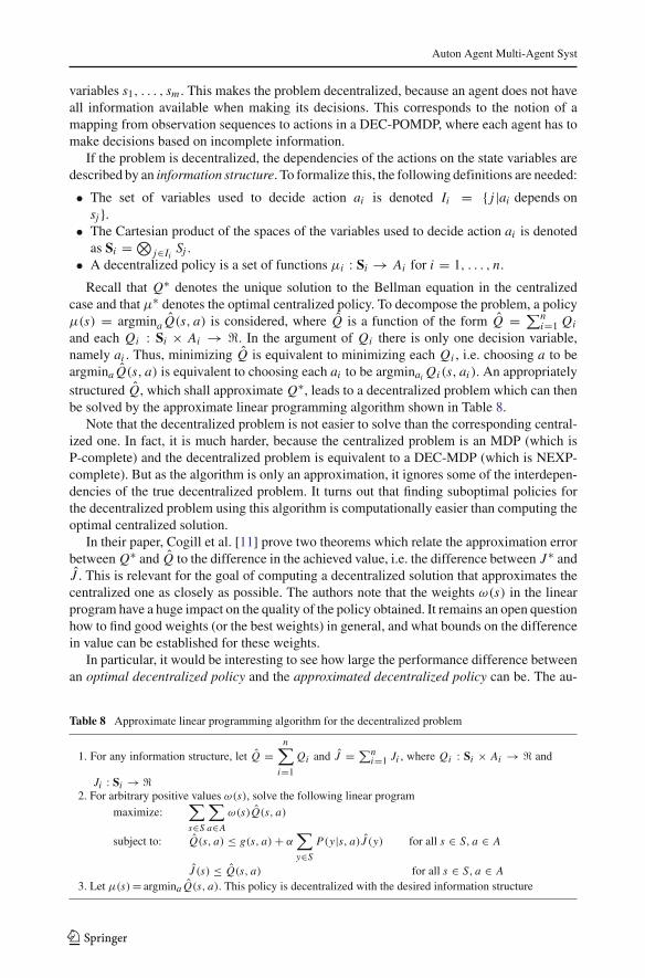
Auton Agent Multi-Agent Syst
variables s1, . . . , sm. This makes the problem decentralized, because an agent does not haveall information available when making its decisions. This corresponds to the notion of amapping from observation sequences to actions in a DEC-POMDP, where each agent has tomake decisions based on incomplete information.
If the problem is decentralized, the dependencies of the actions on the state variables aredescribed by an information structure. To formalize this, the following definitions are needed:
• The set of variables used to decide action ai is denoted Ii = {j |ai depends onsj }.• The Cartesian product of the spaces of the variables used to decide action ai is denoted
as Si =⊗j∈Ii Sj .
• A decentralized policy is a set of functions µi : Si → Ai for i = 1, . . . , n.
Recall that Q∗ denotes the unique solution to the Bellman equation in the centralizedcase and that µ∗ denotes the optimal centralized policy. To decompose the problem, a policyµ(s) = argminaQ(s, a) is considered, where Q is a function of the form Q = ∑n
i=1Qi
and each Qi : Si × Ai → �. In the argument of Qi there is only one decision variable,namely ai . Thus, minimizing Q is equivalent to minimizing each Qi , i.e. choosing a to beargminaQ(s, a) is equivalent to choosing each ai to be argminaiQi(s, ai). An appropriatelystructured Q, which shall approximateQ∗, leads to a decentralized problem which can thenbe solved by the approximate linear programming algorithm shown in Table 8.
Note that the decentralized problem is not easier to solve than the corresponding central-ized one. In fact, it is much harder, because the centralized problem is an MDP (which isP-complete) and the decentralized problem is equivalent to a DEC-MDP (which is NEXP-complete). But as the algorithm is only an approximation, it ignores some of the interdepen-dencies of the true decentralized problem. It turns out that finding suboptimal policies forthe decentralized problem using this algorithm is computationally easier than computing theoptimal centralized solution.
In their paper, Cogill et al. [11] prove two theorems which relate the approximation errorbetweenQ∗ and Q to the difference in the achieved value, i.e. the difference between J ∗ andJ . This is relevant for the goal of computing a decentralized solution that approximates thecentralized one as closely as possible. The authors note that the weights ω(s) in the linearprogram have a huge impact on the quality of the policy obtained. It remains an open questionhow to find good weights (or the best weights) in general, and what bounds on the differencein value can be established for these weights.
In particular, it would be interesting to see how large the performance difference betweenan optimal decentralized policy and the approximated decentralized policy can be. The au-
Table 8 Approximate linear programming algorithm for the decentralized problem
1. For any information structure, let Q =n∑i=1
Qi and J = ∑ni=1 Ji , where Qi : Si × Ai → � and
Ji : Si → �2. For arbitrary positive values ω(s), solve the following linear program
maximize:∑s∈S
∑a∈A
ω(s)Q(s, a)
subject to: Q(s, a) ≤ g(s, a)+ α∑y∈S
P (y|s, a)J (y) for all s ∈ S, a ∈ A
J (s) ≤ Q(s, a) for all s ∈ S, a ∈ A3. Let µ(s)= argminaQ(s, a). This policy is decentralized with the desired information structure
123

Auton Agent Multi-Agent Syst
thors do not compare the empirical results of their algorithm with any other decentralizedalgorithm. A comparison between the bounded policy iteration algorithm and this algorithmwould thus be useful, in order to better evaluate the two different approaches.
The authors illustrate their approach with an example of load balancing among a collectionof queues. The goal is to keep the load at each queue as small as possible. Jobs arrive and areprocessed with a certain probability<1. If one of the queues overflows, a penalty incurs. Thequeues are networked, which enables them to pass a job to one of the neighboring queues ateach time step. The problem is decentralized, as every queue only observes its own backlogas well as the backlogs of its immediate neighbors. The local policies for each queue arestrategies concerning whether to pass a job to one of the neighbors or not, depending on thecurrent backlog status.
For this problem, theQi’s are defined such that each queue’s action is only dependent onthe current backlog of itself and its immediate neighbors at a given time step. This decentral-ization of the problem, however, is suboptimal, because an optimal decentralized solutionwould have to consider entire histories of observations. This is illustrated by an easy examplewith five queues, as shown in Fig. 13.
The arcs indicate incoming jobs and jobs that are passed from one queue to its neighbor.As one can see, at time step 1, queue number 1 passes one job to queue number 2. Fur-thermore, new jobs for queues 1, 2 and 3 arrive. Looking at queue number 3 at time step 2,it would be reasonable to pass a job to one of its neighbors. Considering only the currentbacklog status of its neighbors results in a tie, as both neighbors have a backlog of 2. Thus,the algorithm—only considering the current state—is unable to compute the optimal action.Obviously, if the algorithm would consider the history of observations, it could infer that inthe last time step queue number 1 had passed a job to queue number 2 and that it is thus bestto pass the job to queue number 4 instead of queue number 2. The lack of such considerationfor history illustrates one weakness of the algorithm.
In fact, it is possible to incorporate history into the algorithm, by increasing the state space.A more important question, however, is whether approximating a decentralized problem bytrying to approximate the optimal centralized solution is a reasonable approach. The problemis that the imposed information structure, i.e. the newQi’s, might not make any sense for cer-tain problems. In such cases, solving the linear program with thoseQi’s might yield a resultthat is far from the optimal decentralized solution. For the load balancing problem, the defi-nition of aQi that considers a local view of the problem still makes sense, i.e. optimizing thebacklog locally does somehow optimize the global reward. However, this obviously relies ona special structure of the problem, namely that the coupling between non-adjacent queues is
Fig. 13 An example loadbalancing problem, illustratingthe importance of observationhistory
123
Auton Agent Multi-Agent Syst
weak. Thus, the decentralized version of the problem is very close to the centralized one, and itmakes sense to approximate the centralized solution. For other problems, where the local viewof an agent says little if anything about the global state of the problem, the approach will notgenerally be suitable. In such cases, the value achieved by the algorithm can be arbitrarily bad.
6 Decomposition techniques
As shown in Sect. 2.3.2, even decentralized problems with joint full observability (DEC-MDPs) are NEXP-complete. The high complexity is due to the various ways multiple agentsmight influence each other’s states, observations and rewards. The approximation techniqueconsidered in Sect. 5.3 exploits specific structures in the decentralized process and lowersthe running time of a corresponding algorithm by reducing/ignoring some of the interdepen-dencies found in the problem under consideration. A similar approach has been developed byGoldman and Zilberstein [20]. The important observation is that many decentralized prob-lems have some structure influencing the “level of decentralization,” as discussed in Sect.2.5.1. For example, the special case of a goal-oriented DEC-MDP with independent tran-sitions and observations, with a single global goal state and uniform costs is P-complete[19]. Obviously, not all decentralized problems fall into such special classes, but many onlyviolate the membership conditions slightly. Thus, the idea of decomposing a decentralizedproblem into multiple single-agent MDPs can serve as a useful basis for finding a feasibleapproximate algorithm. To deal with the decentralized nature of the problem, Goldman andZilberstein [20] introduce the notion of communication-based decomposition mechanisms,which involve a communication policy that determines when agents solving individual MDPsshould synchronize their knowledge.
The technical details of this approach are quite involved and are beyond the scope of thisstudy. However, because it offers yet another approach to decentralized decision making, wesummarize the main ideas below. In Sect. 6.1, communication-based decomposition mecha-nisms are introduced. Sect. 6.2 presents the formal framework of decentralized semi-Markovdecision problems that serves as a basis for the associated algorithms. Because finding anoptimal decomposition mechanism for the general case is very hard, the focus turns to morespecific sub-classes of decomposition mechanisms in Sect. 6.3, leading to more efficientalgorithms.
6.1 Communication-based decomposition mechanisms
As discussed in Sect. 2.5.1, even problems with independent transitions and observationsare still hard to solve, because the reward can be dependent on multiple agents and mightnot be decomposable into several independent reward functions. Furthermore, even goal-oriented DEC-MDPs do not necessarily decompose into multiple independent local goals;however, there remains a distinct sub-class with polynomial complexity. Thus, Goldmanand Zilberstein [20] concentrate on finite-horizon goal-oriented problems with independenttransitions and observations and direct communication. The general idea is to let the agentsoperate separately for certain periods of time until they need/want to re-synchronize. Obvi-ously, these periods of separation may sacrifice some possible value, but the benefit is in thelower computational complexity of the single agent problems. Obviously, this is only bene-ficial if the whole decomposition algorithm also has a low complexity. Furthermore, such adecomposition mechanism is required to be complete in that there must exist a communicationpolicy that guarantees the agents will reach one of the global goals whenever possible.
123

Auton Agent Multi-Agent Syst
The agents’ separate phases of execution are defined using temporally abstracted sequencesof actions. These sequences, called options, include a deterministic single-agent policy, ter-minal actions that correspond to communication messages, and a set of initiation states:
Definition 51 (Options) An option for an agent i is given by a tuple opti = 〈π : Si × τ →Ai ∪, I ⊆ Si〉, where
• Si is the set of local states of agent i.• τ is the number of time steps since the process was started.• Ai is the set of agent i’s actions.• is the set of communication messages.• I is the initiation set for the option, i.e. the set of states in which the agent can start the
option.
Note that once an agent executes one of its options, it follows its local policy determinis-tically until it terminates the option by sending a communication message to all other agents.The only way that an option can be terminated earlier is when (a) the time limit T is reachedor (b) another agent sends a communication message. A joint exchange of messages betweenagents is assumed, making it possible to reveal the global state of the system to all agents. Asdiscussed earlier, it is normally too costly for agents to communicate after every time step.The challenge for the decomposition mechanism is to compute the states at which the agentscan act separately, and when it is necessary to re-synchronize.
Definition 52 (Communication-based decomposition mechanism) A communication-baseddecomposition mechanism CDM is a function from any global state of the decentralizedproblem to multiple single agent policies, i.e. CDM : S → (Opt1,Opt2, . . . , Optn).
Obviously, such a mechanism generally only approximates the optimal decentralized jointpolicy. To find the best mechanism, one must search over all possible mechanisms. For twoagents, this requires search over all possible pairs of local single-agent policies and com-munication policies. The best mechanism then is the best approximation (that can be foundthrough decomposition) for the decentralized problem. As we see in the next section, com-puting optimal mechanisms can be very complex. Thus, Sect. 6.3 turns to an easier sub-classof mechanisms that are computationally tractable.
6.2 Decentralized semi-Markov decision problems
The formal framework has to be modified slightly to work with options instead of basic agentactions. Based on an underlying DEC-MDP with direct communication, a goal-orienteddecentralized SMDP with direct communication can be defined. The crucial point is thecomputation of the sets of individual and temporally abstracted actions that are used to buildthe options for each agent. Computing a decomposition mechanism for a DEC-MDP can beframed as a semi-Markov decision problem in the following way:
Definition 53 (GO-DEC-SMDP-COM) A factored finite-horizon goal-oriented DEC-SMDP-COM over an underlying goal-oriented DEC-MDP-COM, DMC, is a tuple 〈DMC,Opt1,Opt2, . . . , Optn, P
N, RN 〉, where:
• DMC is a standard DEC-MDP-COM with components S, , C, {�i}, P , O, T .• Opti is the set of actions available to agent i. It comprises the possible options for
agent i, terminating necessarily with a communication act: opti = 〈π : Si × τ →Ai ∪, I ⊆ Si〉.
123

Auton Agent Multi-Agent Syst
• PN(s′, t + N |s, t, opt1, . . . , optn) is the probability that the system reaches state s′ af-ter N time units (t + N ≤ T ), when at least one option terminates (necessarily with acommunication act).• RN(s, t, opt1, opt2, . . . , optn, s′, t + N) is the expected reward obtained by the systemN time steps after agents start options opt1, . . . , optn in state s at time t , when at leastone terminates its option with a communication act (resulting in termination of the otheragents’ options).
The course of events in the semi-Markov decision process has changed compared to theDEC-MDP. At the beginning of the execution of an option, all agents have full observabilityof the state (as opposed to joint fully observability). Their local policy is a mapping fromglobal states to options. After the first option of one agent terminates, all agents communicate,leading to joint exchange of messages and thus full observability of the global state. Since theglobal state is revealed every time the agents have to choose new options, the choice of localpolicies no longer depends on histories of observations. In fact, only the global state and sys-tem time are important: δi : S× τ → Opti . A joint policy is a tuple of local policies, one foreach agent. Intuitively, optimally solving a decentralized semi-Markov decision problem withtemporally abstracted actions (i.e. solving for an optimal mechanism) is equivalent to solvinga multi-agent MDP (MMDP, see Definition 40), as shown by Goldman and Zilberstein [20].
Theorem 12 A GO-DEC-SMDP-COM is equivalent to a multi-agent MDP.
This may seem counterintuitive, since multi-agent MDPs are P-complete as opposed toDEC-MDPs, which are NEXP-complete. To clarify, the input to this problem now includes avery high number of possible options for each agent. Each option can be represented as a tree,with depth at most T and branching factor at most S. IfA is the set of domain actions availableto the agent, this results in more than |A||S|T possible assignments of primitive domain actions,and thus a double exponential number of possible options. Solving the problem requires com-puting the best option for each agent for each global state. This results in the same doubleexponential complexity as does the original problem. Naturally, any algorithm solving thisproblem optimally needs double exponential time in the worst case (see also the multi-stepbackup policy-iteration algorithm in [20]). As the number of possible options leads to suchhigh complexity, a restricted class of options is now considered. Using these goal-orientedoptions significantly reduces the size of the search space and lowers the overall complexity.
6.3 GO-DEC-SMDP-COM with local goal-oriented behavior
The basic idea presented in this section is to find a mapping from global goals to local goals.That is, with local goal-oriented behavior, there is no need to consider the complete set ofpossible options for each agent. However, not every goal-oriented DEC-MDP automaticallydecomposes into local goal-oriented behavior for each agent. The question of how to generatelocal goals from a given global goal is beyond this study. We simply assume here that a setof local goal states is provided for each agent i, denoted Gi , where Gi ⊆ Si . This set mustinclude the components of the global goal states in G. But in addition, it may also includeother local states from Si , which will serve as temporary local goals. Given these local goalstates, goal-oriented options can be defined as follows:
Definition 54 (Goal-oriented option) Let πopti (si , t) be the policy of an option opti . Let Tbe some time limit. If there exists an optimal policy δ : Si → Ai that minimizes the costto some goal state component gi then opti is goal-oriented if for every state si and t < T ,
123

Auton Agent Multi-Agent Syst
πopti (si , t) = δ(si) and πopti (si , T ) ∈ . It is assumed that the agents have the capability ofexecuting a NOP action, which incurs zero cost and has no transition effect, when they arein some goal state component gi .
Now, the decomposition mechanism has to map each global state to a tuple of goal-orientedoptions and a period of time k. After the agents execute their options for k time steps theyre-synchronize, even if they have not reached their local goals. After exchanging messages,the global state is revealed and new goal-oriented options can be assigned.
The optimal decomposition mechanism now has to find the best mapping from globalstates to goal-oriented options. But once a local goal for agent i has been assigned, thepolicy πgi can be computed independently by optimally solving its local process MDPi =(Si, Pi, Ri, Gi , T ), which can be done in polynomial time. Intuitively, this makes possiblepolynomial time decomposition mechanisms. No longer do all possible options have to beconsidered—instead, the mechanism can focus on the possible local goal states. Indeed,Goldman and Zilberstein [20] present an algorithm based on backup policy-iteration thatcomputes the optimal mechanism based on local goal-oriented behavior and that is polyno-mial in the size of the state space. See their paper for the details of the algorithm and thecorresponding convergence and complexity proofs.
Obviously, an approach based on local goal-oriented behavior is not suitable for every kindof problem. For some problems, the dependence between the agents is so strong (possibly onlythrough the reward function) that every local goal assignment can lead to arbitrarily bad solu-tions. Note that this is the same problem as with the approximate dynamic programming ap-proach discussed in Sect. 5.3. For other problems, however, these techniques make much moresense, and can actually make solving some larger problems possible. In their paper, Goldmanand Zilberstein [20] choose the meeting under uncertainty example to illustrate their approach.In this domain it is reasonable to assign local goals (which are meeting points on a grid) andto communicate from time to time (to get updated information about where the other agentis). For these kind of problems, their algorithms prove to be suitable. Additional algorithmsare presented for situations in which the mapping from global states to single agent behaviorsis already given. In that case, the problem reduces to computing an optimal communicationpolicy.
7 Summary and comparison of algorithms
This section summarizes the characteristics of all the multi-agent planning algorithmsdescribed in this paper. It illustrates the different approaches taken over the past 5 yearsand points out their advantages and disadvantages. First, the algorithms for solving finite-horizon DEC-POMDPs are presented. Then, Sect. 7.2 presents all the algorithms for theinfinite-horizon case.
7.1 Algorithms for finite-horizon DEC-POMDPs
Algorithm Dynamic Programming for DEC-POMDPsAuthors Bernstein et al. [8]Solution quality OptimalSolution technique Bottom-up dynamic programming and iterated elimination of dominated strategiesAdvantages Can exploit specific DEC-POMDP structure of the problemDisadvantages Cannot exploit initial state, runs out of memory quickly
123

Auton Agent Multi-Agent Syst
Algorithm Multi-agent A∗: heuristic search for DEC-POMDPsAuthors Szer et al.[48]Solution quality OptimalSolution technique Top-down A∗-search in the space of joint policiesAdvantages Can exploit an initial state, could use domain-specific knowledge for the heu-
ristic function (when available)Disadvantages Cannot exploit specific DEC-POMDP structure, can at best solve problems with
horizon 1 greater than problems that can be solved via brute force search (inde-pendent of heuristic)
Algorithm Joint equilibrium-based search for policiesAuthors Nair et al. [26]Solution quality ApproximateSolution technique Computation of reachable belief states, dynamic programming, improving pol-
icy of one agent while holding the others fixedAdvantages Avoids unnecessary computation by only considering reachable
belief statesDisadvantages Suboptimal solutions: finds only local optima
Algorithm Approximate solutions for POSGs with common payoffsAuthors Emery-Montemerlo et al. [15]Solution quality ApproximateSolution technique Online algorithm: usage of a series of smaller Bayesian games to approximate
the POSG, matches local agent observations with type profile space in an onlineway
Advantages Interleaves planning with executing, which reduces computational complexity,scales moderately well with problem size
Disadvantages Suboptimal solutions: one-step lookahead reduces solution quality
Algorithm (Improved) Memory-bounded dynamic programmingAuthors Seuken and Zilberstein [42,43]Solution quality ApproximateSolution technique Combines top-down heuristics with bottom-up DP, uses heuristics to identify a
bounded set of relevant belief points and observationsAdvantages Keeps a bounded number of policy trees in memory and as a result has only
polynomial complexity in the time horizonDisadvantages Suboptimal solutions: trade-off between number of policy trees and solution
quality
Algorithm Communication-based decomposition mechanismAuthors Goldman and Zilberstein [20]Solution quality ApproximateSolution technique Decomposition into multiple MDPs and computation of a communication policyAdvantages Exploits structure and takes into account the “level of decentralization,” scales
moderately well for some problemsDisadvantages Limited to those problems that bear special structure
Generally, comparing the performance of different algorithms requires at least that theybe tested on the same machine, and implemented in the same programming language. Thisissue, however, is less of a problem for DEC-POMDPs because the double exponential timecomplexity dominates any linear speed-ups due to different implementations or machines.In fact, so far the challenge has not so much been finding the fastest or best algorithm fora given problem, but finding one that can solve even small benchmark problems for hori-zons larger than 3 or 4. Except for MBDP, all algorithms, whether optimal or approximate,cannot solve standard benchmark problems for horizons larger than 10. Table 9 presents aperformance comparison of all off-line planning algorithms for finite-horizon DEC-POM-DPs for which experimental results on the multi-agent tiger problem have been reported.Shown are the solution values achieved for each horizon. A “?” indicates that the algorithm
123

Auton Agent Multi-Agent Syst
Table 9 Performancecomparison of the differentalgorithms on the multi-agenttiger problem
Horizon DP MAA∗ JESP MBDP
2 −4.00 −4.00 −4.00 −4.003 5.19 5.19 −6.00 5.194 – 4.80 ? 4.805 – – ? 5.386 – – ? 9.917 – – ? 9.678 – – – 9.429 – – – 12.5710 – – – 13.491,000 – – – 819.01100,000 – – – 78252.18
could compute a solution for this horizon, but the achieved value was not reported in thecorresponding paper. A “–” indicates that the algorithm ran out of time or memory for thishorizon.
7.2 Algorithms for Infinite-Horizon DEC-POMDPs
Algorithm Policy iteration for infinite-horizon DEC-POMDPsAuthors Bernstein [5]Solution quality ε-OptimalSolution technique Representation of policies using correlated joint controllers, exhaustive
backups and value-preserving transformationAdvantages Converges to the optimal solution in the limitDisadvantages Computationally intractable due to memory requirements
Algorithm Bounded policy iteration for DEC-POMDPsAuthors Bernstein et al. [7]Solution quality ApproximateSolution technique Representation of policies using correlated joint controllers, improving con-
troller of one agent while holding the others fixedAdvantages Limited memory fixed ahead of time, polynomial time complexity per iter-
ation, allows for correlated randomness, monotonic value improvement forall initial state distributions
Disadvantages Suboptimal solutions: gets stuck in local optima
Algorithm An optimal best-first search algorithm for solving infinite-horizon DEC-POMDPs
Authors Szer and Charpillet [46]Solution quality ApproximateSolution technique Representation of policies using deterministic finite state-controllers, A∗-
search in the space of controllersAdvantages Finds optimal deterministic finite state controller for a given sizeDisadvantages Suboptimal solutions: deterministic finite state controllers achieve signifi-
cantly lower solution values than stochastic controllers
Algorithm Optimal fixed-size control of decentralized POMDPsAuthors Amato et al. [1]Solution quality ApproximateSolution technique Non-linear programming, representation of policies using stochastic finite
state controllersAdvantages Defines optimal stochastic finite state controller for a given size, optimal
controller can be found for some problemsDisadvantages NLPs are more complex than normal LPs, optimal solution cannot always
be found
123

Auton Agent Multi-Agent Syst
Algorithm Approximate dynamic programming for decentralized systemsAuthors Cogill et al. [11]Solution quality ApproximateSolution technique Linear programming using Q-functionsAdvantages Algorithm guarantees a bound on value-loss depending on the approximation
errorDisadvantages Algorithms seeks to approximate the optimal centralized solution, which
can lead away from the optimal decentralized solution
8 Conclusion and open research questions
We have examined the problem of sequential decision making for multiple cooperativeagents in decentralized settings. These problems are much harder than single-agent prob-lems (MDP, POMDP) or their centralized multi-agent variants (MMDP, MPOMDP) becausein a decentralized setting each individual agent may have different partial knowledge aboutthe other agents and about the current state of the world. Five different formal frameworks tomodel the problem were presented: DEC-POMDPs, MTDPs, DEC-POMDP-COMs, COM-MTDPs, and I-POMDPs. The relationships between these models have presented several openquestions. In Sect. 2, we proved formally that the first four models are all equivalent—theyare all NEXP-complete. It is widely believed that optimal algorithms for these models requiredouble exponential time in the worst case. The orthogonal I-POMDP model is more expres-sive in that it allows the modeling of non-cooperative agents, but it leads to non-computableagent functions in the general case. We showed that even its approximate variant, namely thefinitely-nested I-POMDP model, likely requires double exponential time in the worst case.
These complexity results illustrate the difficulty of the problems under consideration.There is little hope that realistic problem instances can be solved optimally. This has ledto investigation of sub-classes of lower complexity, which we described in Sect. 2.5. Theircomplexity ranges from NEXP to P, and thus some of the most restricted classes are computa-tionally tractable. Sect. 3 illustrates how quickly a naive algorithm for the complete problembecomes intractable even for very small problems. Nevertheless, two non-trivial general algo-rithms have been developed: Dynamic Programming for DEC-POMDPs and the heuristicsearch algorithm MAA∗. Our analysis of the limitations of heuristic search showed that bet-ter heuristics, better ways of enumerating children, and weighted heuristics all have limitedutility, as they cannot yield sufficient savings in runtime to allow for much deeper search.
Both of the optimal algorithms introduced in Sect. 3 quickly run out of time or memory, aproblem that is addressed by the latest approximation techniques, presented in Sect. 4. Whilesome of these algorithms establish certain performance bounds, in general only local optimal-ity can be guaranteed. Value loss can therefore be arbitrarily large, depending on the specificproblem. So far, memory-bounded dynamic programming (MBDP) is the only approximatealgorithm for finite-horizon problems that can solve problems that are significantly largerthan those solved by the optimal methods. The technique of keeping a bounded number ofpolicy tress in memory while doing DP updates seems promising; for the current benchmarkproblems its running time scales well even for time horizons beyond 100,000 steps. Its scala-bility for larger problem instances remains to be examined. Another open research questionis how to manage the trade-off between the number of policy trees and solution quality.
Solution techniques for infinite-horizon problems also present some interesting researchquestions. While the nonlinear programming approach is able to specify the optimal fixed-sizecontroller, solving the resulting NLP to find the optimal solution is generally infeasible. Forthe approximate dynamic programming approach, we discussed the instances for which this
123
Auton Agent Multi-Agent Syst
approach might be suitable and why it fails for other problem classes. A similar discussionof decomposition techniques is presented in Sect. 6. This approach is designed specificallyfor those special classes of problems in which local (goal-oriented) behavior of the agents issuitable.
We have seen that some restricted sub-classes of DEC-POMDPs have worst-case complex-ity significantly lower than NEXP. For example, goal-oriented DEC-MDPs with independenttransitions and observations, a single global goal, and uniform costs are P-complete. Thus, ifthe problem under consideration has this special structure, larger instances can be solved effi-ciently. For less restricted classes, many open research questions still remain. For example, thecomplexity of goal-oriented DEC-POMDPs with independent transitions and observations isunknown. Another open question relates to the impact of correlated randomness in finite-statecontrollers for infinite-horizon DEC-POMDPs. As we have seen, correlation can have a largeimpact on the value achieved by memory-bounded algorithms in decentralized settings. How-ever, a full examination of the utility of correlation, in particular how to manage the tradeoffbetween controller size and the size of the correlation device remains to be completed.
The recently developed approximate algorithms for DEC-POMDPs demonstrate differentdegrees of effectiveness and scalability. Some approaches are still limited to toy problems.Others exhibit better scalability, producing good solutions for significantly large problems.The challenge for future research is to fully understand where complexity can be loweredwithout sacrificing value too much, and how to use the available memory most efficiently indealing with complicated problem instances.
Acknowledgments We thank Daniel Bernstein, Marek Petrik, Martin Allen, Christopher Amato, RaphenBecker, Abdel-Illah Mouaddib, Daniel Szer, François Charpillet, Victor Lesser, and Claudia Goldman for help-ful discussions. We also thank the anonymous reviewers for their helful comments and suggestions. Further-more, we thank the authors of all the papers on the different models and algorithms presented in this study. Thiswork was supported in part by the Air Force Office of Scientific Research (Grant No. FA9550-05-1-0254) andby the National Science Foundation (Grant No. 0535061). Any opinions, findings, conclusions or recommen-dations expressed in this manuscript are those of the authors and do not reflect the views of the US government.
References
1. Amato, C., Bernstein, D., & Zilberstein, S. (2007). Optimizing memory-bounded controllers fordecentralized POMDP. In Proceedings of the Twenty-Third Conference on Uncertainty in ArtificialIntelligence (UAI). Vancouver, Canada, July 2007.
2. Amato, C., Bernstein, D. S., & Zilberstein, S. (2007). Solving POMDPs using quadratically constrainedlinear programs. In Proceedings of the Twentieth International Joint Conference on Artificial Intelligence(IJCAI) (pp. 2418–2424). Hyderabad, India, January 2007.
3. Aström, K. J. (1965). Optimal control of Markov decision processes with incomplete state estimation.Journal of Mathematical Analysis and Applications, 10, 174–205.
4. Becker, R., Zilberstein, S., Lesser, V., & Goldman, C. V. (2004). Solving transition independent decen-tralized Markov decision processes. Journal of Artificial Intelligence Research (JAIR), 22, 423–455.
5. Bernstein, D. S. (2005). Complexity analysis and optimal algorithms for decentralized decision making.PhD thesis, Department of Computer Science, University of Massachusetts Amherst, Amherst, MA.
6. Bernstein, D. S., Givan, R., Immerman, N., & Zilberstein, S. (2002). The complexity of decentralizedcontrol of Markov decision processes. Mathematics of Operations Research, 27(4), 819–840.
7. Bernstein, D. S., Hansen, E. A., & Zilberstein, S. (2005). Bounded policy iteration for decentralizedPOMDPs. In Proceedings of the Nineteenth International Joint Conference on Artificial Intelligence(IJCAI) (pp. 1287–1292). Edinburgh, Scotland, July 2005.
8. Bernstein, D. S., Zilberstein, S., & Immerman, N. (2000). The complexity of decentralized control ofMarkov decision processes. In Proceedings of the Sixteenth Conference on Uncertainty in ArtificialIntelligence (UAI) (pp. 32–37). Stanford, California, June 2000.
123

Auton Agent Multi-Agent Syst
9. Beynier, A., & Mouaddib, A. (2006). An iterative algorithm for solving constrained decentralized Markovdecision processes. In Proceedings of the Twenty-First National Conference on Artificial Intelligence(AAAI) (pp. 1089–1094). Boston, MA, July 2006.
10. Boutilier, C. (1996). Planning, learning and coordination in multiagent decision processes. In Proceedingsof the Conference on Theoretical Aspects of Rationality and Knowledge (pp. 195–210). De ZeeuwseStromen, The Netherlands.
11. Cogill, R., Rotkowitz, M., van Roy, B., & Lall, S. (2004). An approximate dynamic programmingapproach to decentralized control of stochastic systems. In Proceedings of the Allerton Conference onCommunication, Control, and Computing (pp. 1040–1049). Urbana-Champaign, IL, 2004.
12. de Farias, D. P., & van Roy, B. (2003). The linear programming approach to approximate dynamicprogramming. Operations Research, 51(6), 850–865.
13. Doshi, P., & Gmytrasiewicz, P. J. (2005). A particle filtering based approach to approximating interactivePOMDPs. In Proceedings of the Twentieth National Conference on Artificial Intelligence (AAAI)(pp. 969–974). Pittsburg, Pennsylvania, July 2005.
14. Doshi, P., & Gmytrasiewicz, P. J. (2005). Approximating state estimation in multiagent settings usingparticle filters. In Proceedings of the Fourth International Joint Conference on Autonomous Agents andMulti-Agent Systems (AAMAS) (pp. 320–327). Utrecht, Netherlands, July 2005.
15. Emery-Montemerlo, R., Gordon, G., Schneider, J., & Thrun, S. (2004). Approximate solutions for partiallyobservable stochastic games with common payoffs. In Proceedings of the Third International Joint Confer-ence on Autonomous Agents and Multi-Agent Systems (AAMAS) (pp. 136–143). New York, NY, July 2004.
16. Gmytrasiewicz, P. J., & Doshi, P. (2005). A framework for sequential planning in multiagent settings.Journal of Artificial Intelligence Research JAIR), 24, 49–79.
17. Goldman, C. V., Allen, M., & Zilberstein, S. (2007). Learning to communicate in a decentralizedenvironment. Autonomous Agents and Multi-Agent Systems, 15(1), 47–90.
18. Goldman, C. V., & Zilberstein, S. (2003). Optimizing information exchange in cooperative multi agentsystems. In Proceedings of the Second International Joint Conference on Autonomous Agents andMulti-Agent Systems (AAMAS) (pp. 137–144). Melbourne, Australia, July 2003.
19. Goldman, C. V., & Zilberstein, S. (2004). Decentralized control of cooperative systems: Categorizationand complexity analysis. Journal of Artificial Intelligence Research (JAIR), 22, 143–174.
20. Goldman, C. V., & Zilberstein, S. (2004). Goal-oriented DEC-MDPs with direct communication.Technical Report 04-44, Department of Computer Science, University of Massachusetts Amherst.
21. Hansen, E. A. (1998). Finite-memory control of partially observable systems. PhD thesis, Departmentof Computer Science, University of Massachuetts Amherst.
22. Hansen, E. A., Bernstein, D. S., & Zilberstein, S. (2004). Dynamic programming for partially observablestochastic games. In Proceedings of the Nineteenth National Conference on Artificial Intelligence (AAAI)(pp. 709–715). San Jose, California, July 2004.
23. Kaelbling, L. P., Littmann, M. L., & Cassandra, A. R. (1998). Planning and acting in partially observablestochastic domains. Artificial Intelligence, 101(2), 99–134.
24. Kalai, E., & Lehrer, E. (1993). Rational learning leads to nash equilibrium. Econometrica, 1, 1231–1240.25. Madani, O., Hanks, S., & Condon, A. (2003). On the undecidability of probabilistic planning and related
stochastic optimization problems. Artificial Intelligence, 147(1–2), 5–34.26. Nair, R., Pynadath, D., Yokoo, M., Tambe, M., & Marsella, S. (2003). Taming decentralized POMDPs:
Towards efficient policy computation for multiagent settings. In Proceedings of the Eighteenth Interna-tional Joint Conference on Artificial Intelligence (IJCAI) (pp. 705–711). Acapulco, Mexico, August 2003.
27. Nair, R., Varakantham, P., Tambe, M., & Yokoo, M. (2005). Networked distributed POMDPs: Asynthesis of distributed constraint optimization and POMDPs. In Proceedings of the Twentieth NationalConference on Artificial Intelligence (AAAI) (pp. 133–139). Pittsburgh, Pennsylvania, July 2005.
28. Nisan, N., Roughgarden, T., Tardos, E., & Vazirani, V. V. (Eds.). (2007). Algorithmic Game Theory.New York, NY: Cambridge University Press.
29. Ooi, J. M., & Wornell, G. W. (1996). Decentralized control of a multiple access broadcast channel:Performance bounds. In Proceedings of the Thirty-Fifth Conference on Decision and Control (pp.293–298). Kobe, Japan, December 1996.
30. Osborne, M. J., & Rubinstein, A. (1994). A course in game theory. Cambridge, MA: The MIT Press.31. Papadimitriou, C. H. (1994). Computational complexity. Reading, MA: Addison Wesley.32. Papadimitriou, C. H., & Tsitsiklis, J. N. (1986). Intractable problems in control theory. SIAM Journal on
Control and Optimization, 24(4), 639–654.33. Papadimitriou, C. H., & Tsitsiklis, J. N. (1987). The complexity of Markov decision processes.
Mathematics of Operations Research, 12(3), 441–450.
123

Auton Agent Multi-Agent Syst
34. Parkes, D. C. (2008). Computational mechanism design. In Lecture notes of Tutorials at 10th Conf.on Theoretical Aspectsof Rationality and Knowledge (TARK-05). Institute of Mathematical Sciences,University of Singapore (to appear).
35. Peshkin, L., Kim, K.-E., Meuleau, N., & Kaelbling, L. P. (2000). Learning to cooperate via policy search.In Proceedings of the Sixteenth Conference on Uncertainty in Artificial Intelligence (UAI) (pp. 489–496).Stanford, CA, July 2000.
36. Petrik, M., & Zilberstein, S. (2007). Anytime coordination using separable bilinear programs. In Pro-ceedings of the Twenty-Second Conference on Artificial Intelligence (AAAI) (pp. 750–755). Vancouver,Canada, July 2007.
37. Poupart, P., & Boutilier, C. (2003). Bounded finite state controllers. In Advances in Neural InformationProcessing Systems 16 (NIPS). Vancouver, Canada, December 2003.
38. Puterman, M. L. (1994). Markov decision processes: discrete stochastic dynamic programming. NewYork, NY: Wiley.
39. Pynadath, D. V., & Tambe, M. (2002). The communicative multiagent team decision problem: Analyzingteamwork theories and models. Journal of Artificial Intelligence Research (JAIR), 16, 389–423.
40. Rabinovich, Z., Goldman, C. V., & Rosenschein, J. S. (2003). The complexity of multiagent systems:The price of silence. In Proceedings of the Second International Joint Conference on Autonomous Agentsand Multi-Agent Systems (AAMAS) (pp. 1102–1103). Melbourne, Australia, 2003.
41. Russell, S., & Norvig, P. (2003). Artificial intelligence: A modern approach. Upper Saddle River, NJ:Prentice Hall.
42. Seuken, S., & Zilberstein, S. (2007). Memory-bounded dynamic programming for DEC-POMDPs.In Proceedings of the Twentieth International Joint Conference on Artificial Intelligence (IJCAI) (pp.2009–2015). Hyderabad, India, January 2007.
43. Seuken, S., & Zilberstein, S. (2007). Improved memory-bounded dynamic programming for decentral-ized POMDPs. In Proceedings of the 23rd Conference on Uncertainty in Artificial Intelligence (UAI).Vancouver, Canada, July 2007.
44. Shen, J., Becker, R., & Lesser, V. (2006). Agent interaction in distributed MDPs and its implicationson complexity. In Proceedings of the Fifth International Joint Conference on Autonomous Agents andMulti-Agent Systems (AAMAS). Hakodate, Japan, May 2006.
45. Suzuki, I., & Yamashita, M. (1999). Distributed anonymous mobile robots: Formation of geometricpatterns. SIAM Journal on Computing, 28(4), 1347–1363.
46. Szer, D., & Charpillet, F. (2005). An optimal best-first search algorithm for solving infinite horizonDEC-POMDPs. In Proceedings of the Sixteenth European Conference on Machine Learning (ECML)(pp. 389–399). Porto, Portugal, October 2005.
47. Szer, D., & Charpillet, F. (2006). Point-based dynamic programming for DEC-POMDPs. In Proceedingsof the Twenty-First National Conference on Artificial Intelligence (AAAI) (pp. 1233–1238). Boston, MA,July 2006.
48. Szer, D., Charpillet, F., & Zilberstein, S. (2005). MAA*: A heuristic search algorithm for solvingdecentralized POMDPs. In Proceedings of the Twenty-First Conference on Uncertainty in ArtificialIntelligence (UAI) (pp. 576–583). Edinburgh, Scotland, July 2005.
49. Tambe, M. (1997). Towards flexible teamwork. Journal of Artificial Intelligence Research (JAIR), 7,83–124.
50. Washington, R., Golden, K., Bresina, J., Smith, D. E., Anderson, C., & Smith, T. (1999). Autono-mous rovers for Mars exploration. In Proceedings of the IEEE Aerospace Conference (pp. 237–251).Snowmass, CO, March 1999.
51. Zilberstein, S., Washington, R.,Bernstein, D. S., & Mouaddib, A.-I. (2002). Decision-theoretic control ofplanetary rovers. In Beetz, M., Guibas, L., Hertzberg, J., Ghallab, M., & Pollack, M.E. (Eds.), Advancesin Plan-Based Control of Robotic Agents, Lecture Notes in Computer Science (Vol. 2466, pp. 270–289).Berlin, Germany: Springer.
123