Noname manuscript No.(will be inserted by the editor)

Formalization and Implementation of Modern SAT

Solvers

Filip Maric

Received: date / Accepted: date

Abstract Most, if not all, state-of-the-art complete SAT solvers are complexvariations of the DPLL procedure described in the early 1960’s. Published de-scriptions of these modern algorithms and related data structures are giveneither as high-level (rule-based) transition systems or, informally, as (pseudo)programming language code. The former, although often accompanied with(informal) correctness proofs, are usually very abstract and do not specifymany details crucial for efficient implementation. The latter usually do notinvolve any correctness argument and the given code is often hard to un-derstand and modify. This paper aims at bridging this gap: we present SATsolving algorithms that are formally proved correct, but at the same time theycontain information required for efficient implementation. We use a tutorial,top-down, approach and develop a SAT solver, starting from a simple designthat is subsequently extended, step-by-step, with the requisite series of fea-tures. Heuristic parts of the solver are abstracted away, since they usually donot affect solver correctness (although they are very important for efficiency).All algorithms are given in pseudo-code. The code is accompanied with correct-ness conditions, given in Hoare logic style. Correctness proofs are formalizedwithin the Isabelle theorem proving system and are available in the extendedversion of this paper. The given pseudo-code served as a basis for our SATsolver argo-sat.

This work was partially supported by Serbian Ministry of Science grant 144030.

Filip MaricFaculty of MathematicsUniversity of BelgradeSerbiaE-mail: filip@matf.bg.ac.yu

2

1 Introduction

Propositional satisfiability problem (SAT) is the problem of deciding if there isa truth assignment under which a given propositional formula (in conjunctivenormal form) evaluates to true. It is a canonical NP-complete problem [Coo71]and it holds a central position in the field of computational complexity. SATproblem is also important in many practical applications such as electronicdesign automation, software and hardware verification, artificial intelligence,and operations research. Thanks to recent advances in propositional solving,SAT solvers are becoming a tool suitable for attacking more and more prac-tical problems. Some of the solvers are complete, while others are stochastic.For a given SAT instance, complete SAT solvers can either find a solution (i.e.,a satisfying variable assignment) or show that no solution exists. Stochasticsolvers, on the other hand, cannot prove that an instance is unsatisfiable al-though they may be able to find a solution for certain kinds of large satisfiableinstances quickly. The majority of the state-of-the-art complete SAT solversare based on the branch and backtracking algorithm called Davis-Putnam-Logemann-Loveland, or DPLL [DP60,DLL62]. Starting with the work on theGRASP and SATO systems [MSS99,Zha97], and continuing with Chaff, Berk-Min and MiniSAT [MMZ+01,GN02,ES04], the spectacular improvements inthe performance of DPLL-based SAT solvers achieved in the last years aredue to (i) several conceptual enhancements of the original DPLL procedure,aimed at reducing the amount of explored search space, such as backjumping,conflict-driven lemma learning, and restarts, and (ii) better implementationtechniques, such as the two-watch literals scheme for unit propagation. Theseadvances make it possible to decide the satisfiability of industrial SAT prob-lems with tens of thousands of variables and millions of clauses.

While SAT solvers have become complex, describing their underlying algo-rithms and data structures has become a nontrivial task. Some papers describeconceptual, higher level concepts, while some papers describe system level ar-chitecture with smart implementation techniques and tricks. Unfortunately,there is still a large gap between these two approaches. Higher level presen-tations, although clean and accompanied with correctness proofs, omit manydetails that are vital to efficient solver implementation. Lower level presenta-tions usually give SAT solver algorithms in a form of pseudo-code. The opensource SAT solvers themselves are, in a sense, the most detailed presentationsor specifications of SAT solving techniques. The success of MiniSAT [ES04],and the number of its re-implementations, indicate that detailed descriptionsof SAT solvers are needed and welcome in the community. However, in order toachieve the highest possible level of efficiency, these descriptions are far fromthe abstract, algorithmic level. Often, one procedure in the code contains sev-eral higher level concepts or one higher level algorithm is spread across severalcode procedures. The resulting pseudo-code, although almost identical to theaward winning solvers, is, in our opinion, hard to understand, modify, and rea-son about. This paper is an attempt to bring these two approaches together.We claim that SAT solvers can be implemented so that (i) the code follows

3

higher level descriptions that make the solver easy to understand, maintain,modify, and to prove correct, and (ii) it contains lower level implementationtricks, and therefore achieves high efficiency. We support this claim by (i) ourSAT solver argo-sat, that represents a rational reconstruction of MiniSAT,obeying the given two requirements, and (ii) our correctness proofs (formalizedin Isabelle) for the presented algorithms, accompanying our SAT solver.1

Complicated heuristics (e.g., for literal selection, for determining the ap-propriate clause database size, restart strategy) represent important parts ofmodern SAT solvers and are crucial for solver efficiency. While a great effortis put on developing new heuristics, and researchers compete to find moreand more effective ones, we argue that those can be abstracted from the corepart of the solver (the DPLL algorithm itself) and represented as just a fewadditional function calls (or separated into external classes in object-orientedsetting). No matter how complicated these heuristics are, they do not affectthe solver correctness as long as they meet a several, usually trivial, conditions.Separating the core DPLL algorithm from complicated, heuristic parts of thesolver leads to simpler solver design, and to more reliable and flexible solvers.

In the rest of the paper, we develop the pseudo-code of a SAT solver fromscratch and outline its correctness arguments along the way. We take a top-down approach, starting with the description of a very simple solver, andintroduce advanced algorithms and data structures one by one. The partialcorrectness of the given code is proved using the proof system Isabelle (in theHoare style). Isabelle proof documents containing the proofs of correctness con-ditions are available in [Mar08]. A longer version of this paper, available fromhttp://argo.matf.bg.ac.rs contains these proofs presented in a less formal,but more readable manner. In this paper we do not deal with termination is-sues. Still, it can be shown that all presented algorithms are terminating2.

Overview of the paper. In §2 we briefly describe the DPLL algorithm, presenttwo rule-based SAT solver descriptions, and describe the basics of programverification and Hoare logic. In §3 we introduce the background theory inwhich we will formalize and prove the properties of a modern SAT solver, anddescribe the pseudo-code language used to describe the implementation. Thebulk of the paper is in §4: it contains descriptions of SAT solver algorithmsand data structures and outlines their correctness proofs. We start from thebasic backtrack search (§4.1), then introduce unit propagation (§4.2), back-jumping, clause learning and firstUIP conflict analysis (§4.3), conflict clauseminimization (§4.4), clause forgetting (§4.5), restarts (§4.6), exploiting literalsasserted at zero level of assertion trail (§4.7), and introduce efficient detectionof conflict and unit clauses using watch literals (§4.8, §4.9). In §5 we give ashort history of SAT solver development, and in §6 we draw final conclusions.

1 Web page of argo-sat is http://argo.matf.bg.ac.rs/2 Formal termination proofs of rule-based systems on which our implementation is based

are available in [Mar08].

4

function dpll (F : Formula) : (SAT, UNSAT)

begin

if F is empty then

return SAT

else if there is an empty clause in F then

return UNSAT

else if there is a pure literal l in F then

return dpll(F [l → ⊤])else there is a unit clause [l] in F then

return dpll(F [l → ⊤])else begin

select a literal l occurring in Fif dpll(F [l → ⊤]) = SAT then

return SAT

else

return dpll(F [l → ⊥])end

end

Fig. 1 DPLL algorithm - recursive definition

2 Background

Davis-Putnam-Logemann-Loveland (DPLL) algorithm. Most of the completemodern SAT solvers are based on the DPLL algorithm [DP60,DLL62]. Its re-cursive version is shown in the Figure 1, where F denotes a set of propositionalclauses, tested for satisfiability, and F [l → ⊤] denotes the formula obtainedfrom F by substituting the literal l with ⊤, its opposite literal l with ⊥, andsimplifying afterwards. A literal is pure if it occurs in the formula but its op-posite does not. A clause is unit if it contains only one literal. This recursiveimplementation is practically unusable for larger formulae and therefore it willnot be used in the rest of this paper.

Rule-based SAT solver descriptions. During the last few years, two transi-tion rule systems which model the DPLL-based SAT solvers and related SMTsolvers have been published [NOT06,KG07]. These descriptions define the top-level architecture of solvers as a mathematical object that can be grasped asa whole and fruitfully reasoned about. Both systems are accompanied withpen-and-paper correctness and termination proofs. Although they succinctlyand accurately capture all major aspects of the solvers’ global operation, theyare high level and far from the actual implementations. Both systems modelthe solver behavior as transitions between states. States are determined bythe values of solver’s global variables. These include the set of clauses F , andthe corresponding assertion trail M . Transitions between states are performedonly by using precisely defined transition rules. The solving process is finishedwhen no more transition rules apply (i.e., when final states are reached).

The system given in [NOT06] is very coarse. It can capture many differentstrategies seen in the state-of-the art SAT solvers, but this comes at a price— several important aspects still have to be specified in order to build animplementation based on the given set of rules.

5

Decide:l ∈ F l, l /∈ M

M := M ld

UnitPropag:l ∨ l1 ∨ . . . ∨ lk ∈ F l1, . . . , lk ∈ M l, l /∈ M

M := M lConflict:

C = no cflct l1 ∨ . . . ∨ lk ∈ F l1, . . . , lk ∈ MC := {l1, . . . , lk}

Explain:l ∈ C l ∨ l1 ∨ . . . ∨ lk ∈ F l1, . . . , lk ≺ l

C := C ∪ {l1, . . . , lk} \ {l}Learn:

C = {l1, . . . , lk} l1 ∨ . . . ∨ lk /∈ F

F := F ∪ {l1 ∨ . . . ∨ lk}Backjump:

C = {l, l1, . . . , lk} l ∨ l1 ∨ . . . ∨ lk ∈ F level l > m ≥ level liC := no cflct M := M [m] l

Forget:C = no cflct c ∈ F F \ c � c

F := F \ cRestart:

C = no cflct

M := M [0]

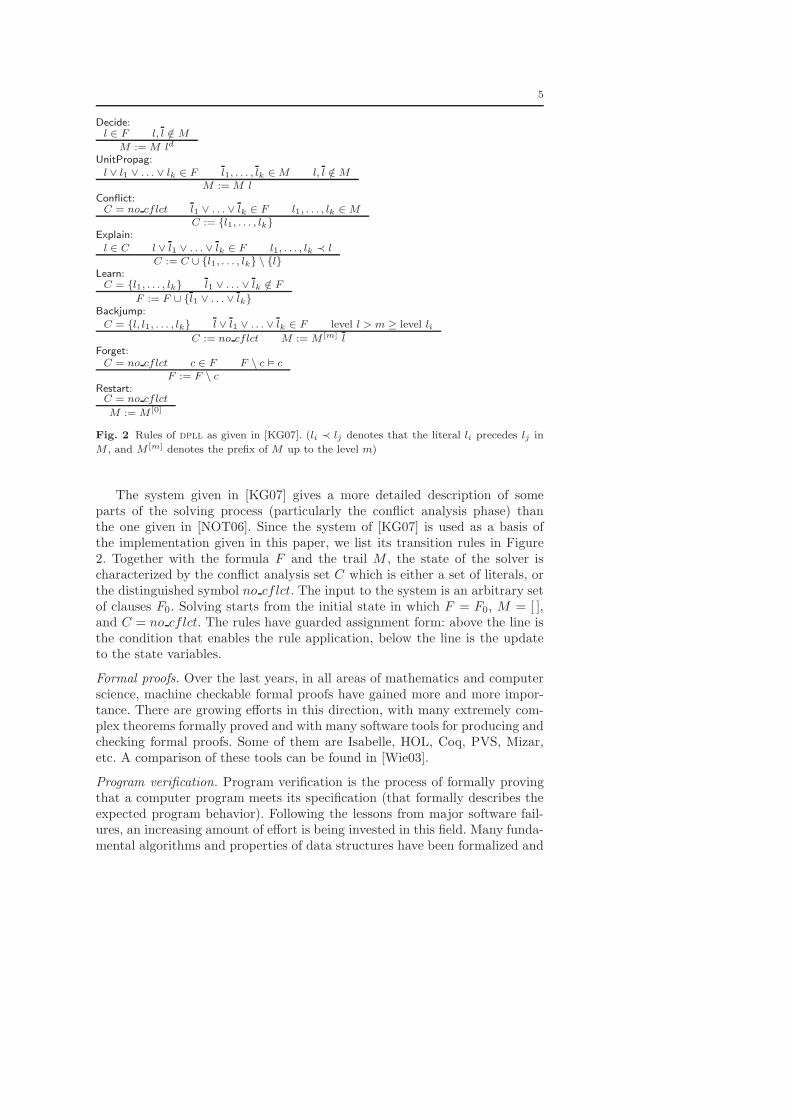
Fig. 2 Rules of dpll as given in [KG07]. (li ≺ lj denotes that the literal li precedes lj in

M , and M [m] denotes the prefix of M up to the level m)

The system given in [KG07] gives a more detailed description of someparts of the solving process (particularly the conflict analysis phase) thanthe one given in [NOT06]. Since the system of [KG07] is used as a basis ofthe implementation given in this paper, we list its transition rules in Figure2. Together with the formula F and the trail M , the state of the solver ischaracterized by the conflict analysis set C which is either a set of literals, orthe distinguished symbol no cflct. The input to the system is an arbitrary setof clauses F0. Solving starts from the initial state in which F = F0, M = [ ],and C = no cflct. The rules have guarded assignment form: above the line isthe condition that enables the rule application, below the line is the updateto the state variables.

Formal proofs. Over the last years, in all areas of mathematics and computerscience, machine checkable formal proofs have gained more and more impor-tance. There are growing efforts in this direction, with many extremely com-plex theorems formally proved and with many software tools for producing andchecking formal proofs. Some of them are Isabelle, HOL, Coq, PVS, Mizar,etc. A comparison of these tools can be found in [Wie03].

Program verification. Program verification is the process of formally provingthat a computer program meets its specification (that formally describes theexpected program behavior). Following the lessons from major software fail-ures, an increasing amount of effort is being invested in this field. Many funda-mental algorithms and properties of data structures have been formalized and

6

verified. Also, a lot of work has been devoted to formalization of compilers,program semantics, communication protocols, security protocols, etc. Formalverification is important for SAT and SMT solvers and the first steps towardsthis direction have been made [KG07,NOT06,Bar03].

Hoare logic. Verification of imperative programs is usually done in Floyd-Hoarelogic [Hoa69], a formal system that provides a set of logical rules in order toreason about the correctness of computer programs with the rigor of mathe-matical logic. The central object in Hoare logic is Hoare triple which describeshow the execution of a piece of code changes the state of a computation. AHoare triple is of the form {P} code {Q}, where P (the precondition) and Q(the postcondition) are formulae of a meta-logic and code is a programminglanguage code. Hoare triple should be read as: ”Given that the assertion Pholds at the point before the code is executed, and the code execution termi-nates, the assertion Q will hold at the point after the code was executed”.

3 Notation and Definitions

In this section we introduce the notation and definitions that will be used inthe rest of the paper.

3.1 Background Theory

In order to reason about the correctness of SAT solver implementations, wehave to formally define the notions we are reasoning about. This formalizationwill be made in higher-order logic of the system Isabelle. Formulae and logicalconnectives of this logic (∧, ∨, ¬, ⇒, ⇔) are written in the usual way. Thesymbol = denotes syntactical identity of two expressions. Function and pred-icate applications are written in prefix form, as in (f x1 . . . xn). Existentialquantifier is written as ∃ and universal quantifier is written as ∀.

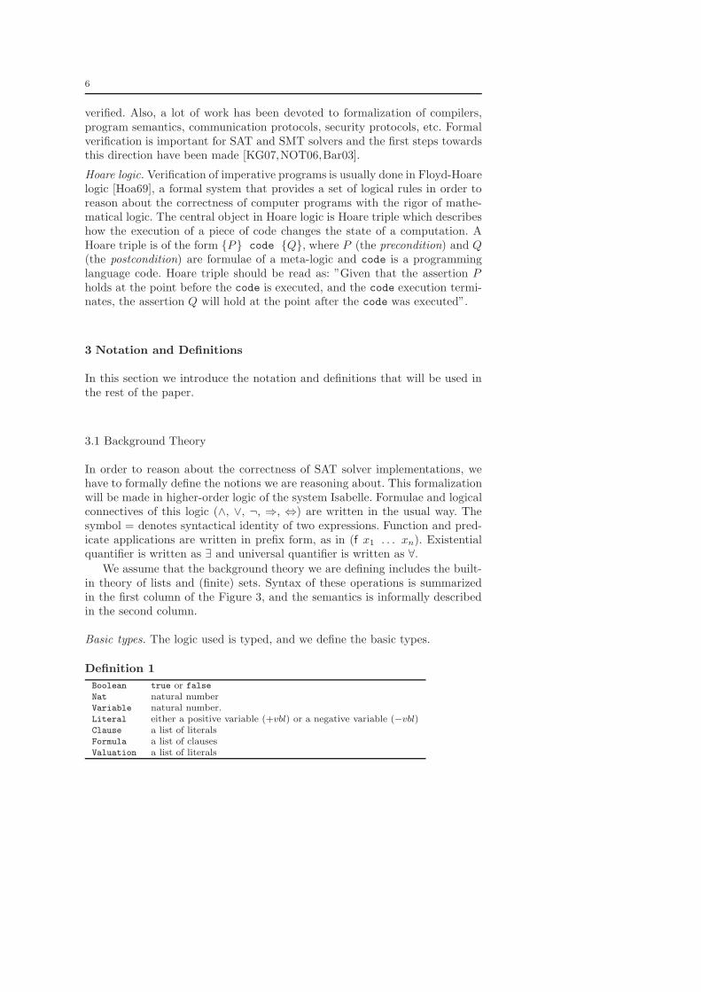
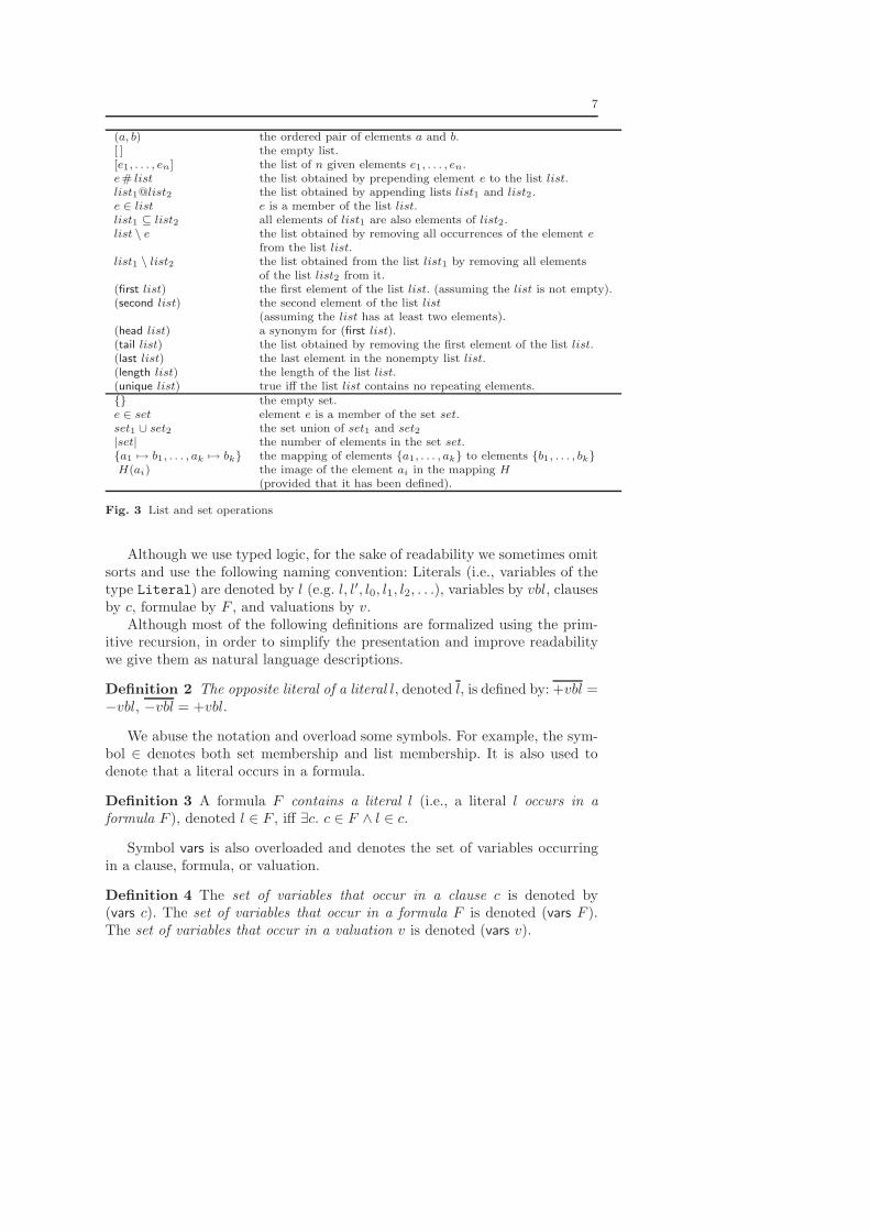
We assume that the background theory we are defining includes the built-in theory of lists and (finite) sets. Syntax of these operations is summarizedin the first column of the Figure 3, and the semantics is informally describedin the second column.

Basic types. The logic used is typed, and we define the basic types.

Definition 1

Boolean true or false

Nat natural numberVariable natural number.Literal either a positive variable (+vbl) or a negative variable (−vbl)Clause a list of literalsFormula a list of clausesValuation a list of literals

7

(a, b) the ordered pair of elements a and b.[ ] the empty list.[e1, . . . , en] the list of n given elements e1, . . . , en.e# list the list obtained by prepending element e to the list list.list1@list2 the list obtained by appending lists list1 and list2.e ∈ list e is a member of the list list.list1 ⊆ list2 all elements of list1 are also elements of list2.list \ e the list obtained by removing all occurrences of the element e

from the list list.list1 \ list2 the list obtained from the list list1 by removing all elements

of the list list2 from it.(first list) the first element of the list list. (assuming the list is not empty).(second list) the second element of the list list

(assuming the list has at least two elements).(head list) a synonym for (first list).(tail list) the list obtained by removing the first element of the list list.(last list) the last element in the nonempty list list.(length list) the length of the list list.(unique list) true iff the list list contains no repeating elements.{} the empty set.e ∈ set element e is a member of the set set.set1 ∪ set2 the set union of set1 and set2|set| the number of elements in the set set.{a1 7→ b1, . . . , ak 7→ bk} the mapping of elements {a1, . . . , ak} to elements {b1, . . . , bk}H(ai) the image of the element ai in the mapping H

(provided that it has been defined).

Fig. 3 List and set operations

Although we use typed logic, for the sake of readability we sometimes omitsorts and use the following naming convention: Literals (i.e., variables of thetype Literal) are denoted by l (e.g. l, l′, l0, l1, l2, . . .), variables by vbl, clausesby c, formulae by F , and valuations by v.

Although most of the following definitions are formalized using the prim-itive recursion, in order to simplify the presentation and improve readabilitywe give them as natural language descriptions.

Definition 2 The opposite literal of a literal l, denoted l, is defined by: +vbl =−vbl, −vbl = +vbl.

We abuse the notation and overload some symbols. For example, the sym-bol ∈ denotes both set membership and list membership. It is also used todenote that a literal occurs in a formula.

Definition 3 A formula F contains a literal l (i.e., a literal l occurs in aformula F ), denoted l ∈ F , iff ∃c. c ∈ F ∧ l ∈ c.

Symbol vars is also overloaded and denotes the set of variables occurringin a clause, formula, or valuation.

Definition 4 The set of variables that occur in a clause c is denoted by(vars c). The set of variables that occur in a formula F is denoted (vars F ).The set of variables that occur in a valuation v is denoted (vars v).

8

The semantics (satisfaction and falsification relations) is defined by:

Definition 5 A literal l is true in a valuation v, denoted v � l, iff l ∈ v.A clause c is true in a valuation v, denoted v � c, iff ∃l. l ∈ c ∧ v � l.A formula F is true in a valuation v, denoted v � F , iff ∀c. c ∈ F ⇒ v � c.

We will write v 2 l to denote that l is not true in v, v 2 c to denote that cis not true in v, and v 2 F to denote that F is not true in v.

Definition 6 A literal l is false in a valuation v, denoted v �¬ l, iff l ∈ v.A clause c is false in a valuation v, denoted v �¬ c, iff ∀l. l ∈ c ⇒ v �¬ l.A formula F is false in a valuation v, denoted v �¬F , iff ∃c. c ∈ F ∧v �¬ c.

We will write v 2¬ l to denote that l is not false in v, v 2¬ c to denote thatc is not false in v, and v 2¬F to denote that F is not false in v. We will saythat l (or c, or F ) is unfalsified in v.

Definition 7 A valuation v is inconsistent, denoted (inconsistent v), iff itcontains both literal and its opposite i.e., ∃l. v � l ∧ v � l. A valuation isconsistent, denoted (consistent v), iff it is not inconsistent.

Definition 8 A model of a formula F is a consistent valuation under whichF is true. A formula F is satisfiable, denoted (sat F ) iff it has a model i.e.,∃v. (consistent v) ∧ v � F

Definition 9 A formula F entails a clause c, denoted F � c, iff c is true inevery model of F . A formula F entails a literal l, denoted F � l, iff l is truein every model of F . A formula F entails valuation v, denoted F � v, iff itentails all its literals i.e., ∀l. l ∈ v ⇒ F � l. A formula F1 entails a formula F2

denoted F1 � F2, if every model of F1 is a model of F2.

Definition 10 Formulae F1 and F2 are logically equivalent, denoted F1 ≡ F2,if any model of F1 is a model of F2 and vice versa, i.e., if F1 � F2, and F2 � F1.

Definition 11 A clause c is unit in a valuation v with a unit literal l, denoted(isUnit c l v) iff l ∈ c, v 2 l, v 2¬ l and v �¬ (c \ l) (i.e., ∀l′. l′ ∈ c ∧ l′ 6= l ⇒v �¬ l′).

Definition 12 A clause c is a reason for propagation of literal l in valuationv, denoted (isReason c l v) iff l ∈ c, v � l, v �¬ (c \ l), and for each literall′ ∈ (c \ l), the literal l′ precedes l in v.

Definition 13 The resolvent of clauses c1 and c2 over the literal l, denoted(resolvent c1 c2 l) is the clause (c1 \ l)@(c2 \ l).

Assertion Trail. In order to build a non-recursive implementation of the dpll

algorithm, the notion of valuation should be slightly extended. During thesolving process, the solver should keep track of the current partial valuation.In that valuation, some literals are called decision literals. Non-decision lit-erals are called implied literals. These check-pointed sequences that represent

9

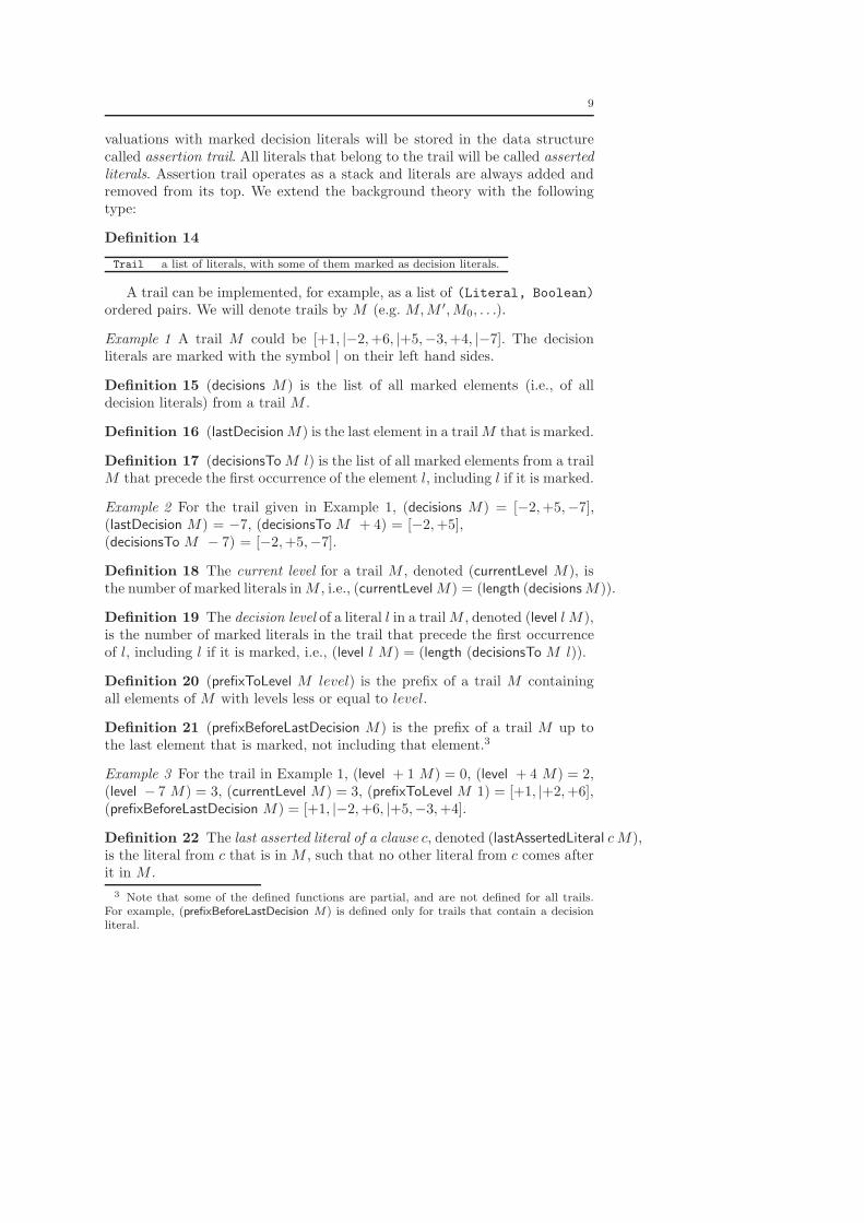
valuations with marked decision literals will be stored in the data structurecalled assertion trail. All literals that belong to the trail will be called assertedliterals. Assertion trail operates as a stack and literals are always added andremoved from its top. We extend the background theory with the followingtype:

Definition 14

Trail a list of literals, with some of them marked as decision literals.

A trail can be implemented, for example, as a list of (Literal, Boolean)

ordered pairs. We will denote trails by M (e.g. M, M ′, M0, . . .).

Example 1 A trail M could be [+1, |−2, +6, |+5,−3, +4, |−7]. The decisionliterals are marked with the symbol | on their left hand sides.

Definition 15 (decisions M) is the list of all marked elements (i.e., of alldecision literals) from a trail M .

Definition 16 (lastDecision M) is the last element in a trail M that is marked.

Definition 17 (decisionsTo M l) is the list of all marked elements from a trailM that precede the first occurrence of the element l, including l if it is marked.

Example 2 For the trail given in Example 1, (decisions M) = [−2, +5,−7],(lastDecision M) = −7, (decisionsTo M + 4) = [−2, +5],(decisionsTo M − 7) = [−2, +5,−7].

Definition 18 The current level for a trail M , denoted (currentLevel M), isthe number of marked literals in M , i.e., (currentLevel M) = (length (decisions M)).

Definition 19 The decision level of a literal l in a trail M , denoted (level l M),is the number of marked literals in the trail that precede the first occurrenceof l, including l if it is marked, i.e., (level l M) = (length (decisionsTo M l)).

Definition 20 (prefixToLevel M level) is the prefix of a trail M containingall elements of M with levels less or equal to level.

Definition 21 (prefixBeforeLastDecision M) is the prefix of a trail M up tothe last element that is marked, not including that element.3

Example 3 For the trail in Example 1, (level + 1 M) = 0, (level + 4 M) = 2,(level − 7 M) = 3, (currentLevel M) = 3, (prefixToLevel M 1) = [+1, |+2, +6],(prefixBeforeLastDecision M) = [+1, |−2, +6, |+5,−3, +4].

Definition 22 The last asserted literal of a clause c, denoted (lastAssertedLiteral c M),is the literal from c that is in M , such that no other literal from c comes afterit in M .

3 Note that some of the defined functions are partial, and are not defined for all trails.For example, (prefixBeforeLastDecision M) is defined only for trails that contain a decisionliteral.

10

Definition 23 The maximal decision level for a clause c in a trail M , denoted(maxLevel c M), is the maximum of all decision levels of all literals from c thatbelong to M , i.e., (maxLevel c M) = (level (lastAssertedLiteral c M) M).

Example 4 Let c is [+4, +6,−3], and M is the trail from the example 1. Then,(maxLevel c M) = 2, and (lastAssertedLiteral c M) = +4.

3.2 Pseudo-code Language

All algorithms in the following text will be specified in a pascal-like pseudo-code language. An algorithm specification consists of a program state decla-ration, followed by a series of function definitions.

The program state is specified by a set of global variables. The state isgiven in the following form, where Typei can be any type of the backgroundtheory.

var

var1 : Type1

. . .vark : Typek

A block is a sequence of statements separated by the symbol ;, where astatement is one of the following:

begin block end

x := expressionif condition then statementif condition then statement else statementwhile condition do statementrepeat statement until conditionfunction name(arg1, ..., argn)

return

Conditions and expressions can include variables, functions calls, and evenbackground theory expressions.

Function definitions are given in the following form, where Typei is thetype of the argument argi, and Type is the return type of the function.

function name (arg1 : Type1, ..., argk : Typek) : Type

begin

blockend

If a function does not return a value, then its return type is omitted. Afunction returns a value by assigning it to a special variable ret. An explicitreturn statement is supported. Parameters are passed by value. If a parameterin the parameter list is marked with the keyword var, then it is passed byreference. Functions marked as const do not change the program state. Inorder to save some space, local variable declarations will be omitted whentheir type is clear from the context.

We allow the use of meta-logic expressions within our algorithm specifica-tions. The reason for this is twofold. First, we want to simplify the presentationby avoiding the need for explicit implementation of some trivial concepts. For

11

example, we assume that lists are supported in the language and we directlyuse the meta-logic notation for the list operations, having in mind that theircorrect implementation can be easily provided. Second, during the algorithmdevelopment, we intentionally leave some conditions at a high level and post-pone their implementation. In such cases, we use meta-logic expressions inalgorithm descriptions to implicitly specify the intended (post)conditions forthe unimplemented parts of the code. For example, we can write if M � Fthen, without specifying how the test for M � F should effectively be imple-mented. These unimplemented parts of the code will be highlighted. Alterna-tively, a function satisfies(M : Trail, F : Formula) : Boolean could beintroduced, which would have the postcondition {ret ⇐⇒ M � F}. Theabove test would then be replaced by if satisfies(M, F) then.

4 SAT Solver Algorithms and Data Structures

In this section, we present SAT solver algorithms and data structures, andoutline their correctness proofs. Our implementation will follow the rules ofthe framework described in [KG07]. We give several variants of SAT solver,labeled as SAT solver v.n. To save space, instead of giving the full code for eachSAT solver variant, we will only print changes with respect to the previousversion of code. These changes will be highlighted. Lines that are added willbe marked by + on the right hand side, and lines that are changed will bemarked by * on the right hand side. Each solver variant contains a function:

function solve (F0 : Formula) : {SAT, UNSAT}

which determines if the given formula F0 is satisfiable or unsatisfiable. Thisfunction sets the global variable satF lag and returns its value.

The partial correctness of the SAT solver v.n is formalized by the followingsoundness theorem:

Theorem 1 SAT solver v.n satisfies the Hoare triple:{⊤} solve(F0) {(satF lag = UNSAT ∧ ¬(sat F0)) ∨ (satF lag = SAT ∧ M � F0)}

This theorem will usually be proved by proving two lemmas:

1. Soundness for satisfiable formulae states that if the solver returns the valueSAT , then the formula F0 is satisfiable.

2. Soundness for unsatisfiable formulae states that if the solver returns thevalue UNSAT , then the formula F0 is unsatisfiable.

Notice that, under the assumption that solver is terminating (which is notproved in this paper), these two soundness lemmas imply solver completeness.

To prove soundness, a set of conditions that each solver variant satisfieswill be formulated. Also, preconditions that have to be satisfied before eachfunction call will be given. All proofs that these conditions are invariants ofthe code and that preconditions are met before each function call are availablein the longer version of this paper.

12

4.1 Basic Backtrack Search

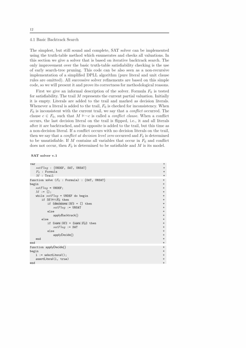
The simplest, but still sound and complete, SAT solver can be implementedusing the truth-table method which enumerates and checks all valuations. Inthis section we give a solver that is based on iterative backtrack search. Theonly improvement over the basic truth-table satisfiability checking is the useof early search-tree pruning. This code can be also seen as a non-recursiveimplementation of a simplified DPLL algorithm (pure literal and unit clauserules are omitted). All successive solver refinements are based on this simplecode, so we will present it and prove its correctness for methodological reasons.

First we give an informal description of the solver. Formula F0 is testedfor satisfiability. The trail M represents the current partial valuation. Initiallyit is empty. Literals are added to the trail and marked as decision literals.Whenever a literal is added to the trail, F0 is checked for inconsistency. WhenF0 is inconsistent with the current trail, we say that a conflict occurred. Theclause c ∈ F0, such that M �¬ c is called a conflict clause. When a conflictoccurs, the last decision literal on the trail is flipped, i.e., it and all literalsafter it are backtracked, and its opposite is added to the trail, but this time asa non-decision literal. If a conflict occurs with no decision literals on the trail,then we say that a conflict at decision level zero occurred and F0 is determinedto be unsatisfiable. If M contains all variables that occur in F0 and conflictdoes not occur, then F0 is determined to be satisfiable and M is its model.

SAT solver v.1

var +

satF lag : {UNDEF, SAT, UNSAT} +

F0 : Formula +

M : Trail +

function solve (F0 : Formula) : {SAT, UNSAT} +

begin +

satF lag = UNDEF; +

M := []; +

while satF lag = UNDEF do begin +

if M �¬F0 then +

if (decisions M) = [] then +

satF lag := UNSAT +

else +

applyBacktrack() +

else +

if (vars M) = (vars F0) then +

satF lag := SAT +

else +

applyDecide() +

end +

end +

function applyDecide() +

begin +

l := selectLiteral(); +

assertLiteral(l, true) +

end +

13

function applyBacktrack() +

begin +

l := (lastDecision M); +

M := (prefixBeforeLastDecision M); +

assertLiteral(l, false) +

end +

function assertLiteral(l : Literal, decision : Boolean) +

begin +

M := M @ [(l, decision)] +

end +

{(vars M) 6= (vars F0)}const function selectLiteral() : Literal +

{(var ret) ∈ (vars F0) ∧ (var ret) /∈ (vars M)}

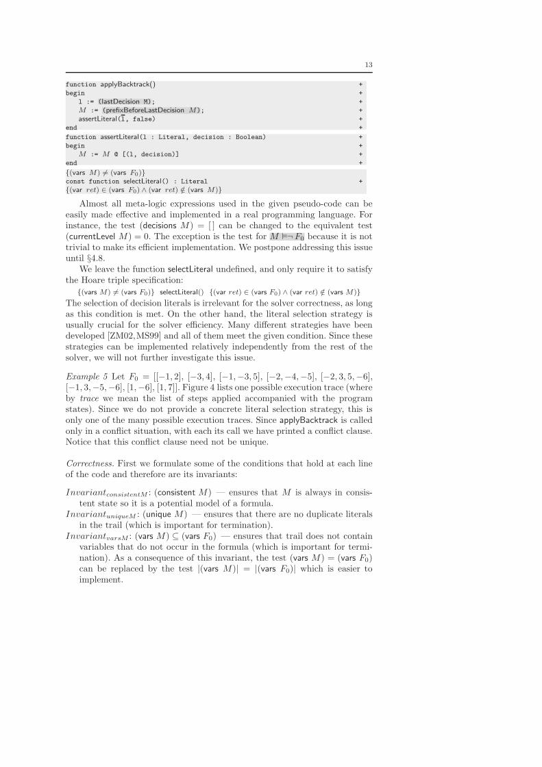
Almost all meta-logic expressions used in the given pseudo-code can beeasily made effective and implemented in a real programming language. Forinstance, the test (decisions M) = [ ] can be changed to the equivalent test(currentLevel M) = 0. The exception is the test for M �¬F0 because it is nottrivial to make its efficient implementation. We postpone addressing this issueuntil §4.8.

We leave the function selectLiteral undefined, and only require it to satisfythe Hoare triple specification:

{(vars M) 6= (vars F0)} selectLiteral() {(var ret) ∈ (vars F0) ∧ (var ret) /∈ (vars M)}

The selection of decision literals is irrelevant for the solver correctness, as longas this condition is met. On the other hand, the literal selection strategy isusually crucial for the solver efficiency. Many different strategies have beendeveloped [ZM02,MS99] and all of them meet the given condition. Since thesestrategies can be implemented relatively independently from the rest of thesolver, we will not further investigate this issue.

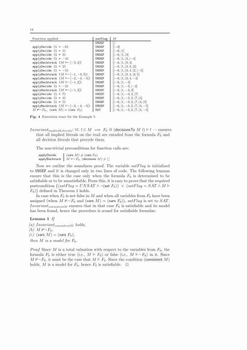
Example 5 Let F0 = [[−1, 2], [−3, 4], [−1,−3, 5], [−2,−4,−5], [−2, 3, 5,−6],[−1, 3,−5,−6], [1,−6], [1, 7]]. Figure 4 lists one possible execution trace (whereby trace we mean the list of steps applied accompanied with the programstates). Since we do not provide a concrete literal selection strategy, this isonly one of the many possible execution traces. Since applyBacktrack is calledonly in a conflict situation, with each its call we have printed a conflict clause.Notice that this conflict clause need not be unique.

Correctness. First we formulate some of the conditions that hold at each lineof the code and therefore are its invariants:

InvariantconsistentM : (consistent M) — ensures that M is always in consis-tent state so it is a potential model of a formula.

InvariantuniqueM : (unique M) — ensures that there are no duplicate literalsin the trail (which is important for termination).

InvariantvarsM : (vars M) ⊆ (vars F0) — ensures that trail does not containvariables that do not occur in the formula (which is important for termi-nation). As a consequence of this invariant, the test (vars M) = (vars F0)can be replaced by the test |(vars M)| = |(vars F0)| which is easier toimplement.

14

Function applied satFlag MUNDEF [ ]

applyDecide (l = −6) UNDEF [|−6]applyDecide (l = 1) UNDEF [|−6, |1]applyDecide (l = 3) UNDEF [|−6, |1, |3]applyDecide (l = −4) UNDEF [|−6, |1, |3, |−4]applyBacktrack (M �¬ [−3, 4]) UNDEF [|−6, |1, |3, 4]applyDecide (l = 2) UNDEF [|−6, |1, |3, 4, |2]applyDecide (l = −5) UNDEF [|−6, |1, |3, 4, |2, |−5]applyBacktrack (M �¬ [−1,−3, 5]) UNDEF [|−6, |1, |3, 4, |2, 5]applyBacktrack (M �¬ [−2,−4,−5]) UNDEF [|−6, |1, |3, 4,−2]applyBacktrack (M �¬ [−1, 2]) UNDEF [|−6, |1,−3]applyDecide (l = −2) UNDEF [|−6, |1,−3, |−2]applyBacktrack (M �¬ [−1, 2]) UNDEF [|−6, |1,−3, 2]applyDecide (l = 7) UNDEF [|−6, |1,−3, 2, |7]applyDecide (l = 4) UNDEF [|−6, |1,−3, 2, |7, |4]applyDecide (l = 5) UNDEF [|−6, |1,−3, 2, |7, |4, |5]applyBacktrack (M �¬ [−2,−4,−5]) UNDEF [|−6, |1,−3, 2, |7, |4,−5]M 2¬F0, (vars M) = (vars F0) SAT [|−6, |1,−3, 2, |7, |4,−5]

Fig. 4 Execution trace for the Example 5

InvariantimpliedLiterals: ∀l. l ∈ M =⇒ F0 @ (decisionsTo M l) � l — ensuresthat all implied literals on the trail are entailed from the formula F0 andall decision literals that precede them.

The non-trivial preconditions for function calls are:

applyDecide (vars M) 6= (vars F0)applyBacktrack M �¬F0, (decisions M) 6= [ ]

Now we outline the soundness proof. The variable satF lag is initializedto UNDEF and it is changed only in two lines of code. The following lemmasensure that this is the case only when the formula F0 is determined to besatisfiable or to be unsatisfiable. From this, it is easy to prove that the requiredpostcondition {(satF lag = UNSAT ∧ ¬(sat F0)) ∨ (satF lag = SAT ∧ M �

F0)} defined in Theorem 1 holds.In case when F0 is not false in M and when all variables from F0 have been

assigned (when M 2¬F0 and (vars M) = (vars F0)), satF lag is set to SAT .InvariantconsistentM ensures that in that case F0 is satisfiable and its modelhas been found, hence the procedure is sound for satisfiable formulae:

Lemma 1 If

(a) InvariantconsistentM holds,(b) M 2¬F0,(c) (vars M) = (vars F0),

then M is a model for F0.

Proof Since M is a total valuation with respect to the variables from F0, theformula F0 is either true (i.e., M � F0) or false (i.e., M �¬F0) in it. SinceM 2¬F0, it must be the case that M � F0. Since the condition (consistent M)holds, M is a model for F0, hence F0 is satisfiable. ⊓⊔

15

When a conflict at decision level zero occurs (when (decisions M) = [] andM �¬F0), satF lag is set to UNSAT . Then, InvariantimpliedLiterals ensuresthat F0 is unsatisfiable, so the procedure is sound for unsatisfiable formulae:

Lemma 2 If

(a) InvariantimpliedLiterals holds,(b) M �¬F0,(c) (decisions M) = [ ],

then F0 is not satisfiable, i.e., ¬(sat F0).

Proof Since (decisions M) = [ ], it holds that (decisionsTo M l) = [ ] and for allliterals l such that l ∈ M , it holds that F0 � l. Thus, the formula F0 is falsein a valuation it entails, so it is unsatisfiable. ⊓⊔

4.2 Unit Propagation

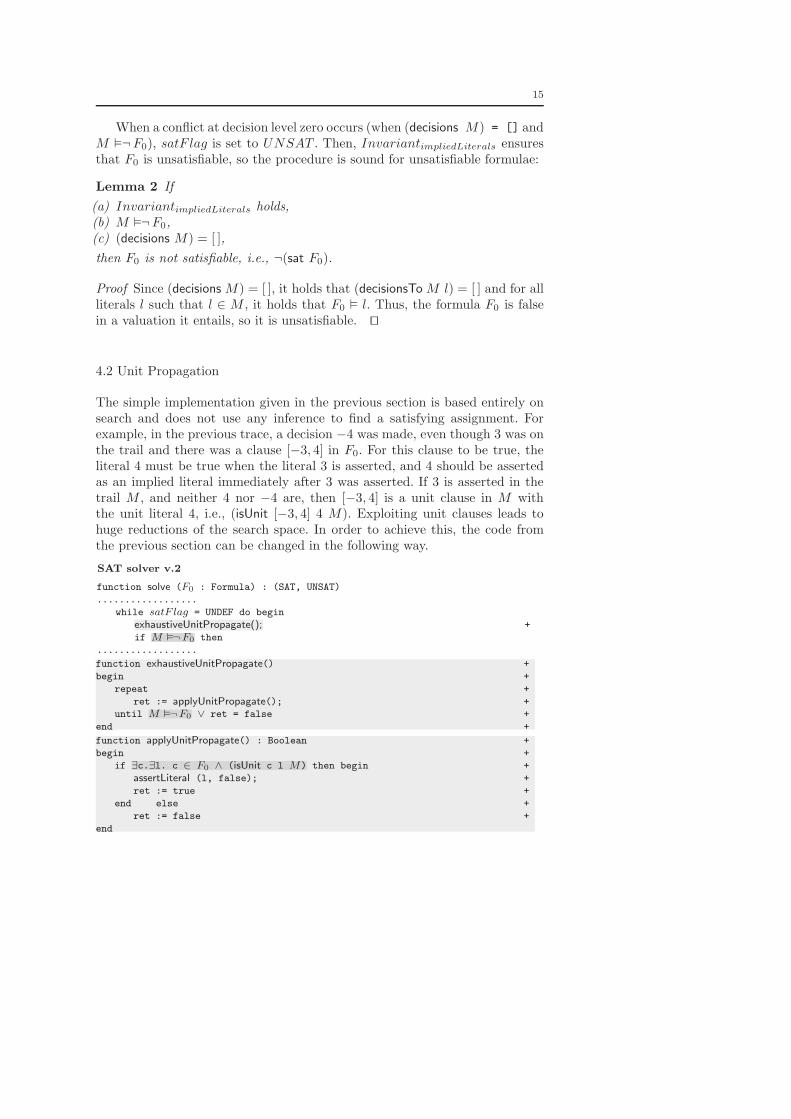
The simple implementation given in the previous section is based entirely onsearch and does not use any inference to find a satisfying assignment. Forexample, in the previous trace, a decision −4 was made, even though 3 was onthe trail and there was a clause [−3, 4] in F0. For this clause to be true, theliteral 4 must be true when the literal 3 is asserted, and 4 should be assertedas an implied literal immediately after 3 was asserted. If 3 is asserted in thetrail M , and neither 4 nor −4 are, then [−3, 4] is a unit clause in M withthe unit literal 4, i.e., (isUnit [−3, 4] 4 M). Exploiting unit clauses leads tohuge reductions of the search space. In order to achieve this, the code fromthe previous section can be changed in the following way.

SAT solver v.2

function solve (F0 : Formula) : (SAT, UNSAT)

..................

while satF lag = UNDEF do begin

exhaustiveUnitPropagate(); +

if M �¬F0 then

..................

function exhaustiveUnitPropagate() +

begin +

repeat +

ret := applyUnitPropagate(); +

until M �¬F0 ∨ ret = false +

end +

function applyUnitPropagate() : Boolean +

begin +

if ∃c.∃l. c ∈ F0 ∧ (isUnit c l M) then begin +

assertLiteral (l, false); +

ret := true +

end else +

ret := false +

end

16

Function applied satFlag MUNDEF [ ]

applyDecide (l = 6) UNDEF [|6]applyUnitPropagate (c = [1,−6], l = 1) UNDEF [|6,1]applyUnitPropagate (c = [−1, 2], l = 2) UNDEF [|6,1, 2]applyDecide (l = 7) UNDEF [|6,1, 2, |7]applyDecide (l = 3) UNDEF [|6,1, 2, |7, |3]applyUnitPropagate (c = [−3, 4], l = 4) UNDEF [|6,1, 2, |7, |3, 4]applyUnitPropagate (c = [−1,−3, 5], l = 5) UNDEF [|6,1, 2, |7, |3, 4, 5]applyBacktrack (M �¬ [−2,−4,−5]) UNDEF [|6,1, 2, |7,−3]applyUnitPropagate (c = [−2, 3, 5,−6], l = 5) UNDEF [|6,1, 2, |7,−3, 5]applyBacktrack (M �¬ [−1, 3,−5,−6]) UNDEF [|6,1, 2,−7]applyDecide (l = 3) UNDEF [|6,1, 2,−7, |3]applyUnitPropagate (c = [−3, 4], l = 4) UNDEF [|6,1, 2,−7, |3, 4]applyUnitPropagate (c = [−1,−3, 5], l = 5) UNDEF [|6,1, 2,−7, |3, 4, 5]applyBacktrack (M �¬ [−2,−4,−5]) UNDEF [|6,1, 2,−7,−3]applyUnitPropagate (c = [−2, 3, 5,−6], l = 5) UNDEF [|6,1, 2,−7,−3, 5]applyBacktrack (M �¬ [−1, 3,−5,−6]) UNDEF [−6]applyDecide (l = 1) UNDEF [−6, |1]applyUnitPropagate (c = [−1, 2], l = 2) UNDEF [−6, |1, 2]applyDecide (l = 7) UNDEF [−6, |1, 2, |7]applyDecide (l = 3) UNDEF [−6, |1, 2, |7, |3]applyUnitPropagate (c = [−3, 4], l = 4) UNDEF [−6, |1, 2, |7, |3, 4]applyUnitPropagate (c = [−1,−3, 5], l = 5) UNDEF [−6, |1, 2, |7, |3, 4, 5]applyBacktrack (M �¬ [−2,−4,−5]) UNDEF [−6, |1, 2, |7,−3]applyDecide (l = 4) UNDEF [−6, |1, 2, |7,−3, |4]applyUnitPropagate (c = [−2,−4,−5], l = −5) UNDEF [−6, |1, 2, |7,−3, |4,−5]M 2¬F0, (vars M) = (vars F0) SAT [−6, |1, 2, |7,−3, |4,−5]

Fig. 5 Execution trace for the Example 6

Example 6 Let F0 be as in Example 5. A possible execution trace is given inFigure 5.

Again, most meta-logic expressions can be easily implemented in a real pro-gramming language. An exception is the test ∃c.∃l. c ∈ F0 ∧ (isUnit c l M),used to detect unit clauses. We postpone addressing this issue until §4.9.

Correctness. Unit propagation does not compromise the code correctness, asthe code preserves all invariants listed in Section 4.1. The proofs of lemmas 1and 2 still apply.

4.3 Backjumping and Learning

A huge improvement in SAT solver development was gained when the simplebacktracking was replaced by the conflict driven backjumping and learning.Namely, two problems are visible from the trace given in Example 6:

1. The series of steps taken after the decision 7 was made showed that neither3 nor −3 are compatible with previous decisions. Because of that, the back-track operation implied that −7 must hold. Then, exactly the same seriesof steps was performed to show that, again, neither 3 nor −3 are compat-ible with previous decisions. Finally, the backtrack operation implied that

17

−6 must hold. A careful analysis of the steps that produced the inconsis-tency would show that the variable 7 is totally irrelevant for the conflict,and the repetition of the process with 7 flipped to −7 was a waste of time.This redundancy was the result of the fact that the backtrack operationalways undoes only the last decision made, regardless of the actual reasonthat caused the inconsistency. The operation of conflict-driven backjumpingwhich is a form of more advanced, non-chronological backtracking, allowssolvers to undo several decisions at once, down to the latest decision literalwhich actually participated in the conflict. This eliminates unnecessaryredundancies in the execution trace.

2. In several steps, the decision 3 was made after the literal 1 was alreadyon the trail. The series of steps taken afterwards showed that these twoare incompatible. Notice that this occurred in two different contexts (bothunder the assumption 6, and under the assumption −6). The fact that 1and 3 are incompatible can be represented by the clause [−1,−3], whichis a logical consequence of F0. If this clause was a part of the formula F ,then it would participate in the unit propagation and it would imply theliteral −3 immediately after 1 occurred on the trail. The clause learningmechanism allows solvers to extend the clause set of the formula duringthe search process with (redundant) clauses implied by F0.

Backjumping is guided by a backjump clause4 (denoted in what followsby C), which is a consequence of the formula F0 and which corresponds tovariable assignment that leads to the conflict. When a backjump clause is con-structed, the top literals from the trail M are removed, until the backjumpclause becomes unit clause in M . From that point, its unit literal is propa-gated and the search process continues. Backjump clauses are constructed inthe process called conflict analysis. This process is sometimes described us-ing a graph-based framework and the backjump clauses are constructed bytraversing the implication graph [ZMMM01]. The conflict analysis process canbe also described as a backward resolution process that starts from the conflictclause and performs a series of resolutions with clauses that are reasons forpropagation of conflict literals [ZM02].

Notice that backtracking can be seen as a special case of backjumping. Thishappens when advanced conflict analysis is not explicitly performed, but thebackjump clause always contains the opposites of all decision literals from M .This clause becomes unit clause when the last decision literal is backtracked,and then it implies the opposite of the backtracked last decision literal.

There are several strategies for conflict analysis [SS96,ZMMM01,ZM02].Their variations include different ways of choosing the clause that guides back-jumping and that is usually learnt. Some strategies allow multiple clauses tobe learnt from a single conflict. Still, most of conflict analysis strategies arebased on the following technique:

– The conflict analysis process starts with a conflict clause itself (the clauseof F that is false in M), and the backjump clause C is initialized to it.

4 Sometimes also called the assertive clause.

18

– Each literal contained in the current backjump clause C is false in thecurrent trail M and is either a decision made by the search procedure, or theresult of some propagation. For each propagated literal l,, there is a clausec that forced this propagation to occur. These clauses are called reasonclauses, and (isReason c l M) holds. Propagated literals from the currentbackjump clause C are then replaced (we say explained) by other literalsfrom reason clauses, continuing the analysis backwards. The explanationstep can be seen as a resolution between the backjump and reason clauses.

– The procedure is repeated until some termination condition is fulfilled,resulting in the final backjump clause.

Different strategies determine termination conditions for the conflict anal-ysis process. We will only describe the one called the first unique implicationpoint (firstUIP), since it is used in most leading SAT solvers and since itoutperforms other strategies on most benchmarks [ZM02]. Using the firstUIPstrategy, the learning process is terminated when the backjump clause containsexactly one literal from the current decision level.

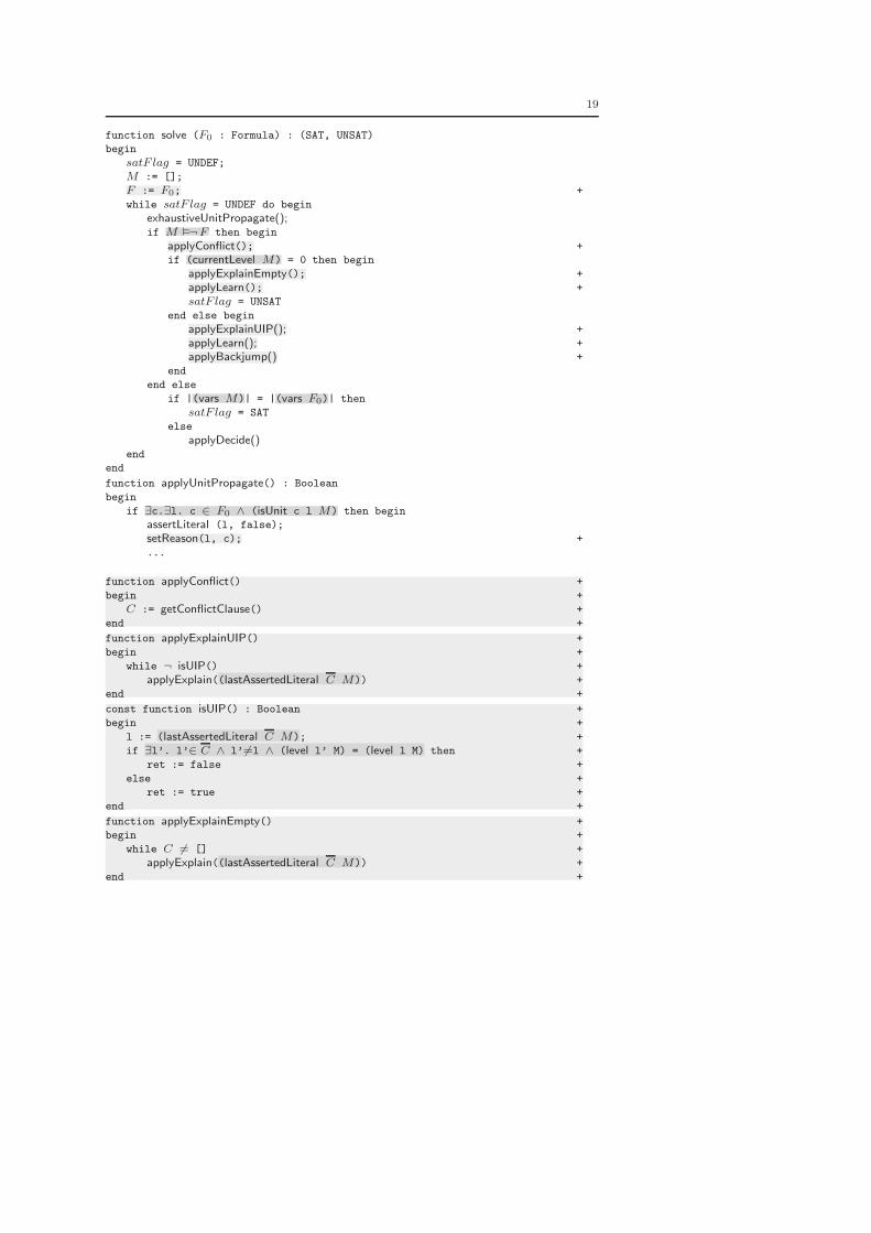
The following version of the solver works similarly to SAT solver v.2 up tothe point when M �¬F i.e., when a conflict occurs. Then, the conflict anal-ysis is performed, implemented through applyConflict and applyExplain func-tions. The function applyConflict initializes the backjump clause C to a conflictclause. The function applyExplain resolves out a literal l from C by performinga single resolution step between C and a clause that is the reason for propa-gation of l. When the conflict is resolved, the solver continues to work as SATsolver v.2.

If a conflict occurs at a decision level other then zero, then a backjumpclause is constructed using the function applyExplainUIP. It iteratively resolvesout the last asserted literal of C using the applyExplain function until C satisfiesthe firstUIP condition. The function applyLearn adds the constructed backjumpclause C to the current clause set F . The function applyBackjump backtracksliterals from the trail M until C becomes a unit clause, and after that assertsthe unit literal of C. Notice that this last step does not have to be done byapplyBackjump, but it can be handled by the function applyUnitPropagate. So,some implementations of applyBackjump omit its last two lines given here.

If a conflict at decision level zero occurs, then the empty clause C is ef-fectively constructed using the function applyExplainEmpty. It always resolvesout the last asserted literal from C by calling applyExplain, until C becomesempty. It is possible to extend the solver with the possibility of generatingresolution proofs for unsatisfiability and this explicit construction of emptyclause makes that process more uniform.

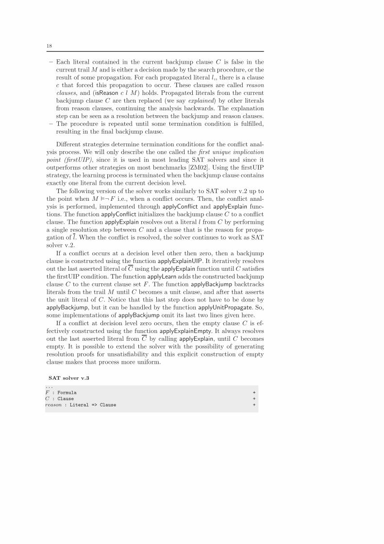
SAT solver v.3

...

F : Formula +

C : Clause +

reason : Literal => Clause +

19

function solve (F0 : Formula) : (SAT, UNSAT)

begin

satF lag = UNDEF;

M := [];

F := F0; +

while satF lag = UNDEF do begin

exhaustiveUnitPropagate();if M �¬F then begin

applyConflict(); +

if (currentLevel M) = 0 then begin

applyExplainEmpty(); +

applyLearn(); +

satF lag = UNSAT

end else begin

applyExplainUIP(); +

applyLearn(); +

applyBackjump() +

end

end else

if |(vars M)| = |(vars F0)| then

satF lag = SAT

else

applyDecide()end

end

function applyUnitPropagate() : Boolean

begin

if ∃c.∃l. c ∈ F0 ∧ (isUnit c l M) then begin

assertLiteral (l, false);

setReason(l, c); +

...

function applyConflict() +

begin +

C := getConflictClause() +

end +

function applyExplainUIP() +

begin +

while ¬ isUIP() +

applyExplain((lastAssertedLiteral C M)) +

end +

const function isUIP() : Boolean +

begin +

l := (lastAssertedLiteral C M); +

if ∃l’. l’∈ C ∧ l’6=l ∧ (level l’ M) = (level l M) then +

ret := false +

else +

ret := true +

end +

function applyExplainEmpty() +

begin +

while C 6= [] +

applyExplain((lastAssertedLiteral C M)) +

end +

20

function applyExplain(l : Literal) +

begin +

reason := getReason(l); +

C := (resolvent C reason l) +

end +

function applyLearn() +

begin +

F = F @ C +

end +

function applyBackjump() +

begin +

l := (lastAssertedLiteral C M); +

level := getBackjumpLevel(); +

M := (prefixToLevel M level); +

assertLiteral(l, false) +

setReason(l, C); +

end +

const function getBackjumpLevel : int +

begin +

l := (lastAssertedLiteral C M); +

if C \ l 6= [] then +

ret := (maxLevel C \ l M) +

else +

ret := 0 +

end +

const function getReason(l : Literal) : Clause +

begin +

ret := reason(l) +

end +

function setReason(l : Literal, c : Clause) +

begin +

reason(l) := c +

end +

{M �¬F}const function getConflictClause() : Clause +

{M �¬ ret}

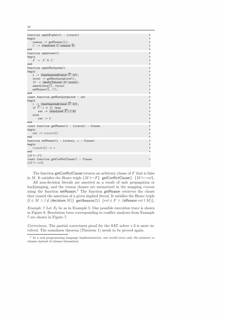
The function getConflictClause returns an arbitrary clause of F that is falsein M . It satisfies the Hoare triple {M �¬F} getConflictClause() {M �¬ ret}.

All non-decision literals are asserted as a result of unit propagation orbackjumping, and the reason clauses are memorized in the mapping reasonusing the function setReason.5 The function getReason retrieves the clausethat caused the assertion of a given implied literal. It satisfies the Hoare triple{l ∈ M ∧ l /∈ (decisions M)} getReason(l) {ret ∈ F ∧ (isReason ret l M)}.

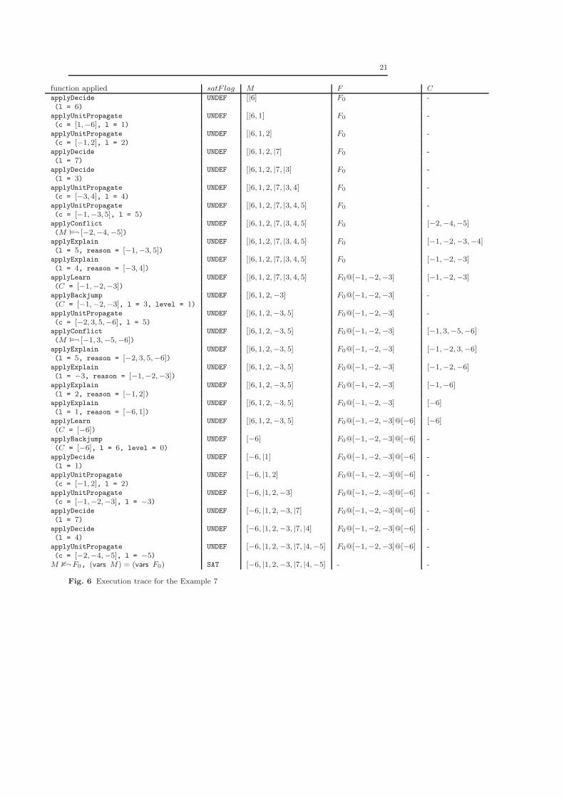
Example 7 Let F0 be as in Example 5. One possible execution trace is shownin Figure 6. Resolution trees corresponding to conflict analyses from Example7 are shown in Figure 7.

Correctness. The partial correctness proof for the SAT solver v.3 is more in-volved. The soundness theorem (Theorem 1) needs to be proved again.

5 In a real programming language implementation, one would store only the pointers toclauses instead of clauses themselves.

21

function applied satF lag M F CapplyDecide UNDEF [|6] F0 -(l = 6)applyUnitPropagate UNDEF [|6, 1] F0 -(c = [1,−6], l = 1)applyUnitPropagate UNDEF [|6, 1, 2] F0 -(c = [−1, 2], l = 2)applyDecide UNDEF [|6, 1, 2, |7] F0 -(l = 7)applyDecide UNDEF [|6, 1, 2, |7, |3] F0 -(l = 3)applyUnitPropagate UNDEF [|6, 1, 2, |7, |3, 4] F0 -(c = [−3, 4], l = 4)applyUnitPropagate UNDEF [|6, 1, 2, |7, |3, 4, 5] F0 -(c = [−1,−3, 5], l = 5)applyConflict UNDEF [|6, 1, 2, |7, |3, 4, 5] F0 [−2,−4,−5](M �¬ [−2,−4,−5])applyExplain UNDEF [|6, 1, 2, |7, |3, 4, 5] F0 [−1,−2,−3,−4](l = 5, reason = [−1,−3, 5])applyExplain UNDEF [|6, 1, 2, |7, |3, 4, 5] F0 [−1,−2,−3](l = 4, reason = [−3, 4])applyLearn UNDEF [|6, 1, 2, |7, |3, 4, 5] F0@[−1,−2,−3] [−1,−2,−3](C = [−1,−2,−3])applyBackjump UNDEF [|6, 1, 2,−3] F0@[−1,−2,−3] -(C = [−1,−2,−3], l = 3, level = 1)applyUnitPropagate UNDEF [|6, 1, 2,−3, 5] F0@[−1,−2,−3] -(c = [−2, 3, 5,−6], l = 5)applyConflict UNDEF [|6, 1, 2,−3, 5] F0@[−1,−2,−3] [−1, 3,−5,−6](M �¬ [−1, 3,−5,−6])applyExplain UNDEF [|6, 1, 2,−3, 5] F0@[−1,−2,−3] [−1,−2, 3,−6](l = 5, reason = [−2, 3, 5,−6])applyExplain UNDEF [|6, 1, 2,−3, 5] F0@[−1,−2,−3] [−1,−2,−6](l = −3, reason = [−1,−2,−3])applyExplain UNDEF [|6, 1, 2,−3, 5] F0@[−1,−2,−3] [−1,−6](l = 2, reason = [−1, 2])applyExplain UNDEF [|6, 1, 2,−3, 5] F0@[−1,−2,−3] [−6](l = 1, reason = [−6, 1])applyLearn UNDEF [|6, 1, 2,−3, 5] F0@[−1,−2,−3]@[−6] [−6](C = [−6])applyBackjump UNDEF [−6] F0@[−1,−2,−3]@[−6] -(C = [−6], l = 6, level = 0)applyDecide UNDEF [−6, |1] F0@[−1,−2,−3]@[−6] -(l = 1)applyUnitPropagate UNDEF [−6, |1, 2] F0@[−1,−2,−3]@[−6] -(c = [−1, 2], l = 2)applyUnitPropagate UNDEF [−6, |1, 2,−3] F0@[−1,−2,−3]@[−6] -(c = [−1,−2,−3], l = −3)applyDecide UNDEF [−6, |1, 2,−3, |7] F0@[−1,−2,−3]@[−6] -(l = 7)applyDecide UNDEF [−6, |1, 2,−3, |7, |4] F0@[−1,−2,−3]@[−6] -(l = 4)applyUnitPropagate UNDEF [−6, |1, 2,−3, |7, |4,−5] F0@[−1,−2,−3]@[−6] -(c = [−2,−4,−5], l = −5)

M 2¬F0, (vars M) = (vars F0) SAT [−6, |1, 2,−3, |7, |4,−5] - -

Fig. 6 Execution trace for the Example 7

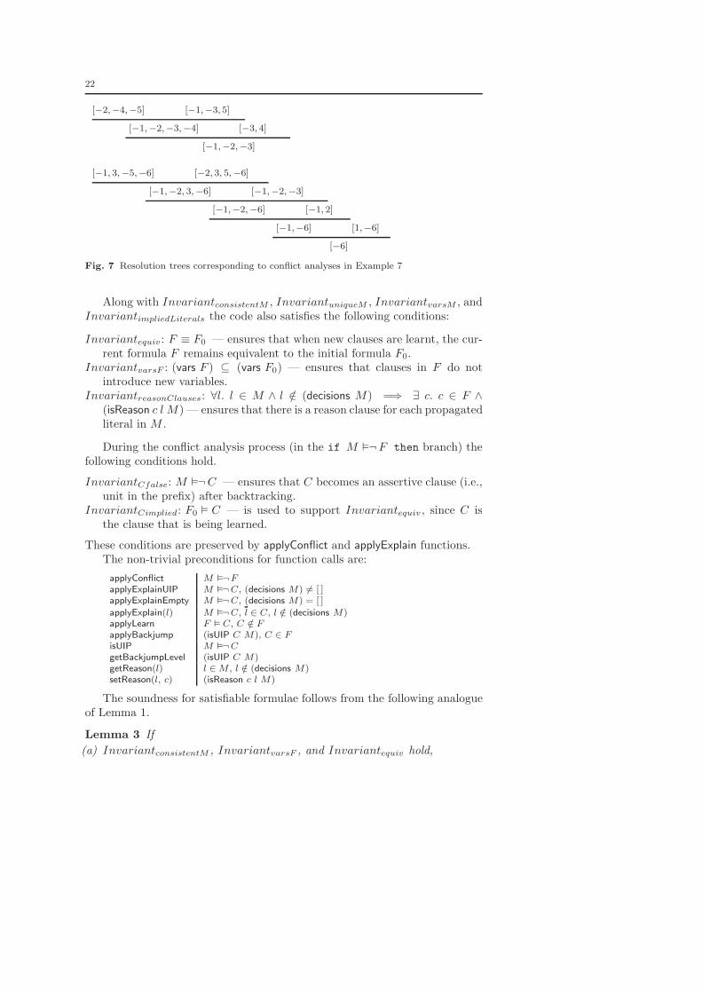
22

[−2,−4,−5] [−1,−3, 5]

[−1,−2,−3,−4] [−3, 4]

[−1,−2,−3]

[−1, 3,−5,−6] [−2, 3, 5,−6]

[−1,−2, 3,−6] [−1,−2,−3]

[−1,−2,−6] [−1, 2]

[−1,−6] [1,−6]

[−6]

Fig. 7 Resolution trees corresponding to conflict analyses in Example 7

Along with InvariantconsistentM , InvariantuniqueM , InvariantvarsM , andInvariantimpliedLiterals the code also satisfies the following conditions:

Invariantequiv : F ≡ F0 — ensures that when new clauses are learnt, the cur-rent formula F remains equivalent to the initial formula F0.

InvariantvarsF : (vars F ) ⊆ (vars F0) — ensures that clauses in F do notintroduce new variables.

InvariantreasonClauses: ∀l. l ∈ M ∧ l /∈ (decisions M) =⇒ ∃ c. c ∈ F ∧(isReason c l M) — ensures that there is a reason clause for each propagatedliteral in M .

During the conflict analysis process (in the if M �¬F then branch) thefollowing conditions hold.

InvariantCfalse: M �¬C — ensures that C becomes an assertive clause (i.e.,unit in the prefix) after backtracking.

InvariantCimplied: F0 � C — is used to support Invariantequiv , since C isthe clause that is being learned.

These conditions are preserved by applyConflict and applyExplain functions.The non-trivial preconditions for function calls are:

applyConflict M �¬FapplyExplainUIP M �¬C, (decisions M) 6= [ ]applyExplainEmpty M �¬C, (decisions M) = [ ]

applyExplain(l) M �¬C, l ∈ C, l /∈ (decisions M)applyLearn F � C, C /∈ FapplyBackjump (isUIP C M), C ∈ FisUIP M �¬CgetBackjumpLevel (isUIP C M)getReason(l) l ∈ M , l /∈ (decisions M)setReason(l, c) (isReason c l M)

The soundness for satisfiable formulae follows from the following analogueof Lemma 1.

Lemma 3 If

(a) InvariantconsistentM , InvariantvarsF , and Invariantequiv hold,

23

(b) M 2¬F ,(c) (vars M) = (vars F0),

then M is a model for F0.

Proof Since (vars F ) ⊆ (vars F0) and (vars M) = (vars F0), it holds that(vars F ) ⊆ (vars M), and M is a total valuation with respect to variablesfrom F . So, the formula F is either true (i.e., M � F ) or false (i.e., M �¬F )in it. Since M 2¬F , it must be the case that M � F . Since the condition(consistent M) holds, M is a model for F . Since F and F0 are logically equiv-alent by Invariantequiv , M is also a model for F0. ⊓⊔

Regarding the soundness for unsatisfiable formulae, an analouge of Lemma2 could be formulated and proved. However, we give a simpler, alternativeproof of soundness for unsatisfiability, that does not use InvariantimpliedLiterals

(in contrast to the given proof of Lemma 2). After a conflict at the decisionlevel zero has been detected (when M �¬F and (decisions M) = [ ]), thefunction applyExplainEmpty is called. It performs a series of applications of theexplain rule, and resolves out all the literals from the conflict clause, leavingthe empty clause C. In this case, the procedure reports unsatisfiability of theformula, if and only if the empty clause has been derived. The postcondition ofapplyExplainEmpty guarantees that C = [ ], and the soundness is a consequenceof InvariantCimplied (i.e., F0 � C), as stated in the following trivial lemma(given without proof).

Lemma 4 If the following conditions hold

(a) C = [ ],(b) F0 � C (i.e., InvariantCimplied holds),

then F0 is unsatisfiable.

Soundness for satisfiability and soundness for unsatisfiability together im-ply Theorem 1 for SAT Solver v.3.

4.3.1 Efficient Data Structures

The code given in §4.3 leaves the function resolvent unspecified. We will nowdescribe how it can be efficiently implemented, roughly following MiniSAT[ES04]. Without a great loss of generality, it is assumed that the conflict clause(and therefore the clause C) contains a literal from the current decision leveli.e., (currentLevel M) = (maxLevel C M). This holds whenever there is aguarantee that no new decisions are made when M �¬F , and, clearly, this isthe case in the implementation we provided.6 It is also reasonable to requirethat the clause C does not contain repeated elements. So, in each resolvent step,when a union of two clauses is created, duplicates have to be removed. In orderto achieve an efficient implementation, instead of ordinary list of literals, somemore suitable representation for the clause C has to be used. We use a map CH

6 We will see that this is an important requirement for the correctness of the two-watchliteral propagation scheme that we explain in §4.9.

24

that maps literals to booleans such that CH(l) = true iff l ∈ C. Notice that thisrepresentation allows constant time check whether a literal is contained in theclause C so it is suitable for a range of operations performed with this clause.When the conflict analysis process is done, the list of literals contained in theclause C can be constructed by traversing the map CH looking for literalswhich are true in it. Notice that this expensive traversal can be avoided usingthe fact that during the firstUIP conflict analysis only the literals from thehighest decision level of C (i.e., the current decision level of M) are explained.So, when a literal from a decision level lower then the current decision levelof M is added into the clause C, it cannot get removed from it until the endof the firstUIP resolution process. Also, since the UIP condition is met at theend of the resolution process, the backjump clause contains exactly one literalfrom the current (highest) decision level. Therefore, it is useful to keep the listCP of the literals from the lower decision levels from C and the last assertedliteral Cl of C, because these two can give the list of literals contained in theclause C at the end, avoiding the traversal of CH . In order to optimize isUIP

check, the procedure also keeps track of the number Cn of literals from thehighest decision level (that is (currentLevel M)).

The list of literals C from §4.3 used in SAT solver v.3, and the variablesCH , CP , Cl and Cn used in SAT solver v.4 are related as follows:

CH(l) = true ⇔ l ∈ C

Cl = (lastAssertedLiteral C M)

l ∈ CP ⇔ l ∈ C ∧ (level l M) < (maxLevel C M)

Cn = |{l : l ∈ C ∧ (level l M) = (maxLevel C M)}|

The following code is a modification of SAT solver v.3 adapted to use thedata structures just described. The clause C (that is its components CH , CP ,Cn) can be changed only by the functions addLiteral and removeLiteral, whileCl is set by findLastAssertedLiteral.

SAT solver v.4...

CH : Literal => Boolean

CP : Clause

Cl : Literal

Cn : nat

...

function applyConflict()begin

CH := {}; +

foreach l : l ∈ getConflictClause() do *

addLiteral(l) *

findLastAssertedLiteral(); +

end

function applyExplainUIP()begin

while ¬ isUIP() do

applyExplain(Cl); *

buildC() +

end

25

function buildC() +

C := CP @ Cl +

end +

const function isUIP() : Boolean

begin

if Cn = 1 then ret := true else ret := false *

end

function applyExplain(l : Literal)

begin

reason := getReason(l);resolve(reason, l) *

findLastAssertedLiteral(); +

end

function resolve(clause : Clause, l : Literal) +

begin +

removeLiteral(l); +

foreach l’: l’ ∈ clause ∧ l’ 6= l do +

addLiteral(l’) +

end +

function applyBackjump()begin

level := getBackjumpLevel();M := (prefixToLevel M level);

assertLiteral(Cl, false) *

setReason(Cl, C); *

end

const function getBackjumpLevel : int

begin

if CP 6= [] then *

ret := (maxLevel CP M) *

else

ret := 0

end

function addLiteral(l : Literal) +

begin +

if CH(l) = false then begin +

CH(l) := true; +

if (level l M) = (currentLevel M) then +

Cn := Cn + 1 +

else +

CP := CP @ l +

end +

end +

function removeLiteral(l : Literal) +

begin +

CH(l) := false; +

if (level l M) = (currentLevel M) then +

Cn := Cn - 1 +

else +

CP := CP \ l +

end +

26

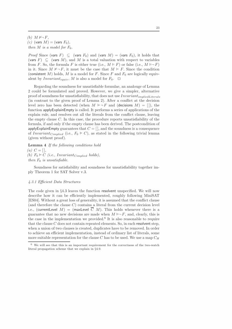
function applied CH7 CP Cl Cn

. . .applyConflict {−2 7→ ⊤,−4 7→ ⊤,−5 7→ ⊤} [−2] 5 2(M �¬ [−2,−4,−5])applyExplain {−1 7→ ⊤,−2 7→ ⊤,−3 7→ ⊤,−4 7→ ⊤} [−1,−2] 4 2(l = 5, reason = [−1,−3, 5])applyExplain {−1 7→ ⊤,−2 7→ ⊤,−3 7→ ⊤} [−1,−2] 3 1(l = 4, reason = [−3, 4])

. . .

Fig. 8 The conflict analysis using efficient data-structures.

function findLastAssertedLiteral() +

begin +

repeat +

Cl := (last M) +

until CH(Cl) = true +

end +

Example 8 Figure 8 show one conflict analysis trace, from Example 7, forM = [|6, 1, 2, |7, |3, 4, 5].

Notice that some minor optimizations can be made in the given code. Forexample, the function resolve is always called with a current level literal asthe clashing literal. Therefore, the call to the generic removeLiteral function,could be replaced by a call to function removeCurrentLevelLiteral that wouldalways be called for a literal at the current level. This would save a check ofthe level of the literal that is being removed. Also, it is possible to changethe map CH , so that it maps variables instead of literals to booleans. In thatcase, l ∈ C would imply that CH(var l) must hold. This change is possible,because invariants (consistent M) and M �¬C imply that C can not be atautological clause i.e., it can not contain both a literal and its opposite. So,since it holds that l ∈ C ⇔ CH(l) = true, for each literal l it must hold thatCH(l) = true ⇒ CH(l) = false.

4.4 Conflict Clause Minimization

In some cases, clauses obtained by the firstUIP heuristic can further be mini-mized. Smaller clauses prune larger parts of the search tree and lead to fasterunit propagation. Several clause minimization techniques have been proposed;as an illustration, we present the subsumption resolution of [ES04]. In Exam-ple 7, the learnt backjump clause is [−1,−2,−3], but since 2 is implied by 1(because of the clause [−1, 2]), one more resolution step could be performedto get a smaller backjump clause [−1,−3].

This variant of SAT solver augments SAT solver v.3.

SAT solver v.5

function solve (F0 : Formula) : (SAT, UNSAT)

..........................

7 For simplicity, literals that map to ⊥ are omitted.

27

applyExplainUIP();applyExplainSubsumption(); +

applyLearn();applyBackjump()

..........................

function applyExplainSubsumption() +

begin +

foreach l: l ∈ C ∧ l /∈ (decisions M) do +

if subsumes(C, getReason(l) \ l) then +

applyExplain(l) +

end +

const function subsumes (c1 : Clause, c2 : Clause) : Boolean +

begin +

if c2 ⊆ c1 then ret := true else ret := false +

end +

The subsumption check has to be carefully implemented so that it does notbecome the bottleneck of this part of the solver. An implementation that usesthe efficient conflict analysis clause representation given in §4.3.1 is availablein the extended version of this paper.

A more advanced conflict clause minimization, based on subsumption, canalso be performed. Namely, the subsumption check fails if the reason clausefor l contains at least one literal l′ different from l that is not in C. However,by following the reason graph backwards for l′, we might find that l′ becametrue as a consequence of assigning only literals present in the conflict clause,in which case l′ can be ignored. If this is true for all literals l′ of the reasonclause that are not in C, then the literal l can still be explained.

4.5 Forgetting

During the solving process with clause learning, the number of clauses in Fincreases. If the number of clauses becomes too large, then the boolean con-straint propagation becomes unacceptably slow and some (redundant) clausesfrom F should be removed. It is necessary to take special care and ensure thatthe reduced formula is still equivalent with the initial formula F0 (i.e., thatInvariantequiv is preserved). Solvers usually ensure this by allowing only theremoval of learnt clauses while the initial clauses never get removed. It is alsorequired that clauses that are reasons for propagation of some literals in Mare not removed (i.e., that InvariantreasonClauses is preserved).

The following modifications can be made to any given clause learning SATsolver (solvers after variant 3).

SAT solver v.6

function solve (F0 : Formula) : (SAT, UNSAT)

..........................

if shouldForget() then +

applyForget() +

applyDecide()..........................

28

function applyForget()begin

newF := [];

foreach c : c ∈ F do

if shouldForget(c) ∧ isLearnt(c) ∧ ¬isReason(c) then

removeClause(c)else

newF := newF @ c;

F := newF

end

{⊤}const function shouldForget() : Boolean +

{⊤}

{⊤}const function shouldForget(Clause : c) : Boolean +

{⊤}

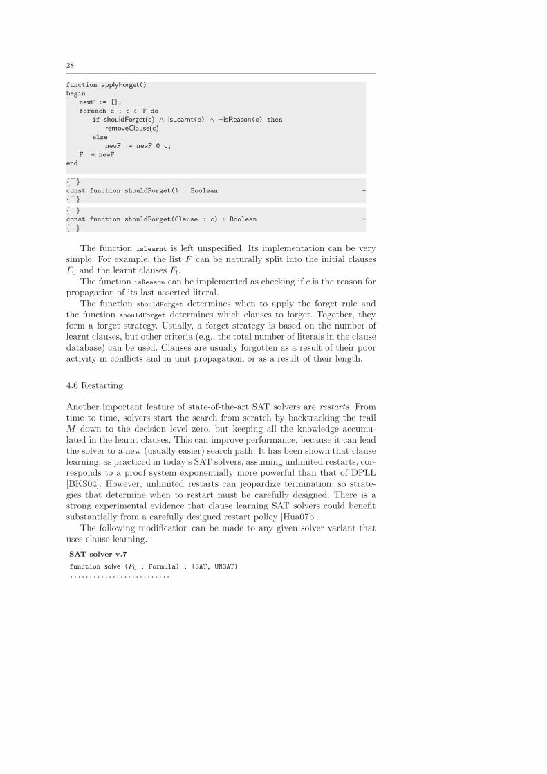
The function isLearnt is left unspecified. Its implementation can be verysimple. For example, the list F can be naturally split into the initial clausesF0 and the learnt clauses Fl.

The function isReason can be implemented as checking if c is the reason forpropagation of its last asserted literal.

The function shouldForget determines when to apply the forget rule andthe function shouldForget determines which clauses to forget. Together, theyform a forget strategy. Usually, a forget strategy is based on the number oflearnt clauses, but other criteria (e.g., the total number of literals in the clausedatabase) can be used. Clauses are usually forgotten as a result of their pooractivity in conflicts and in unit propagation, or as a result of their length.

4.6 Restarting

Another important feature of state-of-the-art SAT solvers are restarts. Fromtime to time, solvers start the search from scratch by backtracking the trailM down to the decision level zero, but keeping all the knowledge accumu-lated in the learnt clauses. This can improve performance, because it can leadthe solver to a new (usually easier) search path. It has been shown that clauselearning, as practiced in today’s SAT solvers, assuming unlimited restarts, cor-responds to a proof system exponentially more powerful than that of DPLL[BKS04]. However, unlimited restarts can jeopardize termination, so strate-gies that determine when to restart must be carefully designed. There is astrong experimental evidence that clause learning SAT solvers could benefitsubstantially from a carefully designed restart policy [Hua07b].

The following modification can be made to any given solver variant thatuses clause learning.

SAT solver v.7

function solve (F0 : Formula) : (SAT, UNSAT)

..........................

29

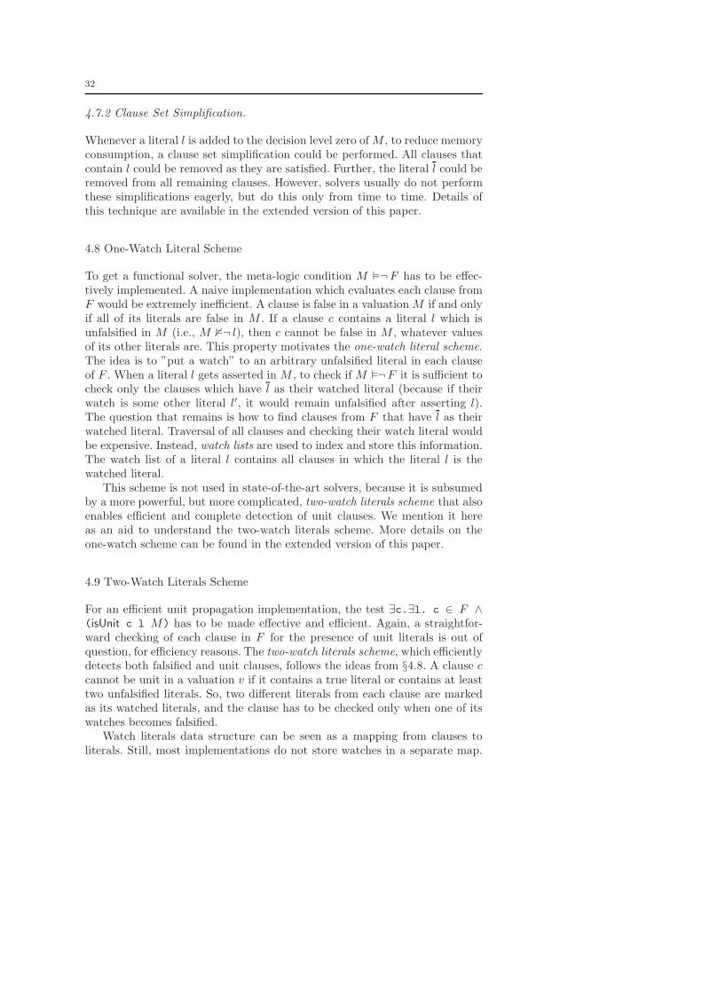
if shouldRestart() then +

applyRestart() +

applyDecide()..........................

function applyRestart() +

begin +

M := (prefixToLevel M 0) +

end +

{⊤}const function shouldRestart() : Boolean +

{⊤}

The function shouldRestart() is intentionally left unspecified and it representsthe restart strategy of the solver. For a survey of restart strategies see, forinstance, [Hua07b].

4.7 Zero Level Literals

Since (level l M) = 0 =⇒ (decisionsTo M l) = [ ], the InvariantimpliedLiterals

ensures that literals at the decision level zero are consequences of the formulaitself. These literals have a special role during the solving process.

4.7.1 Single Literal Clauses

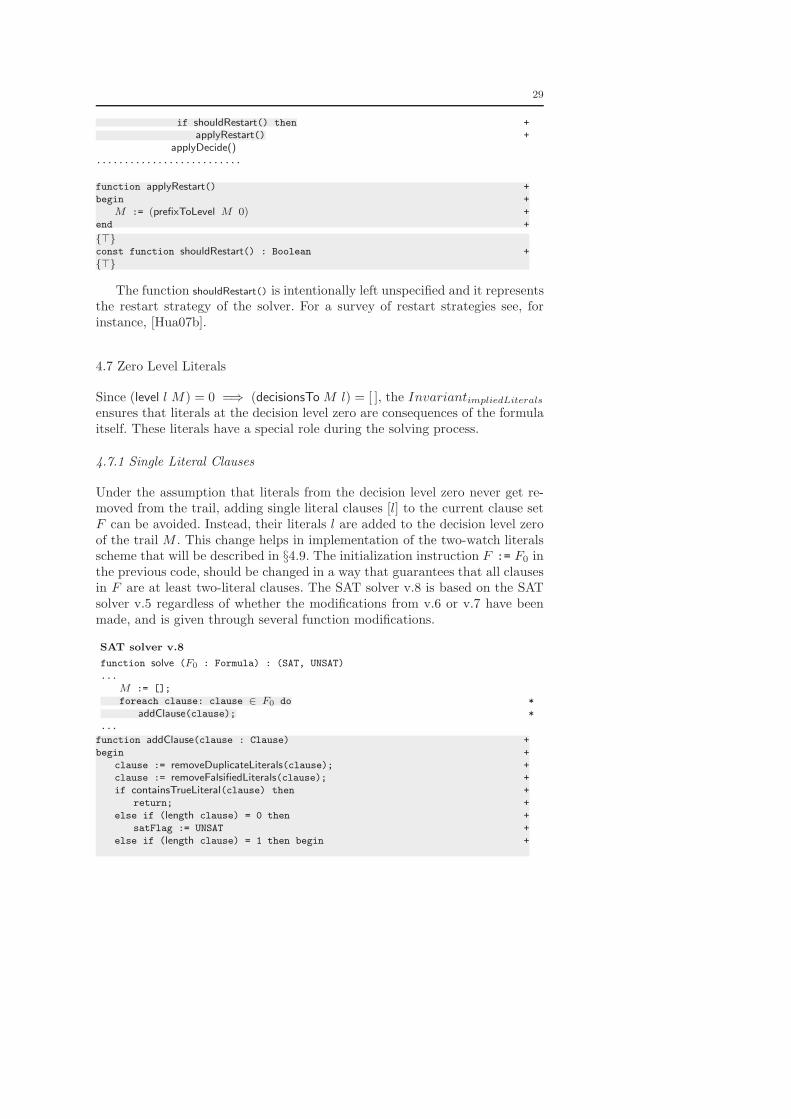
Under the assumption that literals from the decision level zero never get re-moved from the trail, adding single literal clauses [l] to the current clause setF can be avoided. Instead, their literals l are added to the decision level zeroof the trail M . This change helps in implementation of the two-watch literalsscheme that will be described in §4.9. The initialization instruction F := F0 inthe previous code, should be changed in a way that guarantees that all clausesin F are at least two-literal clauses. The SAT solver v.8 is based on the SATsolver v.5 regardless of whether the modifications from v.6 or v.7 have beenmade, and is given through several function modifications.

SAT solver v.8

function solve (F0 : Formula) : (SAT, UNSAT)

...

M := [];

foreach clause: clause ∈ F0 do *

addClause(clause); *

...

function addClause(clause : Clause) +

begin +

clause := removeDuplicateLiterals(clause); +

clause := removeFalsifiedLiterals(clause); +

if containsTrueLiteral(clause) then +

return; +

else if (length clause) = 0 then +

satFlag := UNSAT +

else if (length clause) = 1 then begin +

30

assertLiteral((head clause), false); +

exhaustiveUnitPropagate() +

end else if isTautological(clause) then +

return; +

else +

F := F @ clause +

end +

const function containsTrueLiteral(clause: Clause) : Boolean +

begin +

ret := false; +

foreach l : l ∈ clause do +

if M � l then ret := true +

end +

const function removeDuplicateLiterals(clause : Clause) : Clause +

begin +

ret := []; +

foreach l : l ∈ clause do +

if l /∈ ret then ret := ret @ l; +

end +

const function removeFalsifiedLiterals(clause : Clause) : Clause +

begin +

ret := []; +

foreach l : l ∈ clause do +

if M 2¬ l then ret := ret @ l; +

end +

const function isTautological(c : clause) +

if ∃ l. l∈c ∧ l∈c then ret:=true else ret:=false +

end +

The given initialization procedure also ensures that no clause in F containsduplicate literals or both a literal and its negation. This property is preservedthroughout the code and is another invariant.

Learning should be changed so that it is performed only for clauses withat least two (different) literals:

function applyLearn()begin

if (length C) > 1 then +

F = F @ Cend

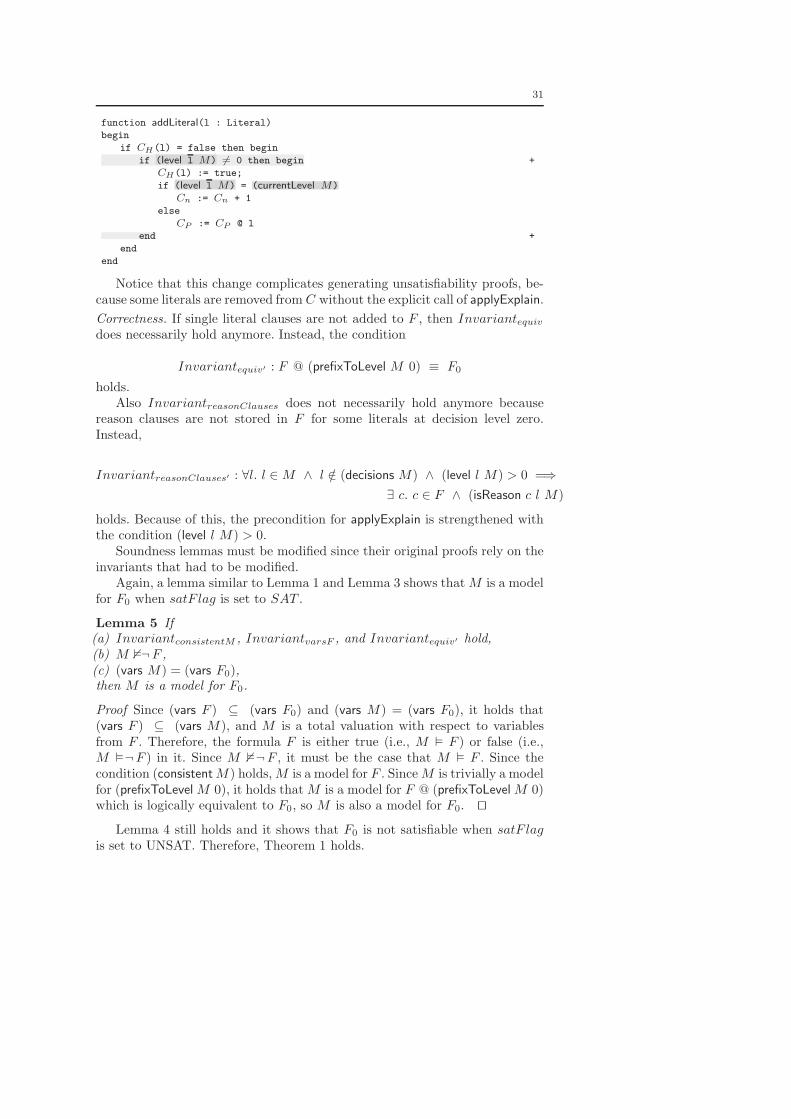
Since learning is not performed for single literal clauses, for some zero levelliterals there is no reason clause stored in F . This means that those literalscannot be explained and removed from C using the applyExplain function (itis still safe to call getReason(l) for all non-decision literals asserted at higherdecision levels). To handle this, backjump clauses are generated so that theydo not contain literals from the decision level zero. These literals are skippedduring the conflict analysis process and applyExplain is modified so that afterits application C becomes (resolvent C c l) \ (prefixToLevel M 0). When usingthe efficient representation of conflict analysis clause, defined in §4.3.1, thefunction addLiteral is modified in the following way.

31

function addLiteral(l : Literal)

begin

if CH(l) = false then begin

if (level l M) 6= 0 then begin +

CH(l) := true;

if (level l M) = (currentLevel M)

Cn := Cn + 1

else

CP := CP @ l

end +

end

end

Notice that this change complicates generating unsatisfiability proofs, be-cause some literals are removed from C without the explicit call of applyExplain.

Correctness. If single literal clauses are not added to F , then Invariantequiv

does necessarily hold anymore. Instead, the condition

Invariantequiv′ : F @ (prefixToLevel M 0) ≡ F0

holds.Also InvariantreasonClauses does not necessarily hold anymore because

reason clauses are not stored in F for some literals at decision level zero.Instead,

InvariantreasonClauses′ : ∀l. l ∈ M ∧ l /∈ (decisions M) ∧ (level l M) > 0 =⇒

∃ c. c ∈ F ∧ (isReason c l M)

holds. Because of this, the precondition for applyExplain is strengthened withthe condition (level l M) > 0.

Soundness lemmas must be modified since their original proofs rely on theinvariants that had to be modified.

Again, a lemma similar to Lemma 1 and Lemma 3 shows that M is a modelfor F0 when satF lag is set to SAT .

Lemma 5 If(a) InvariantconsistentM , InvariantvarsF , and Invariantequiv′ hold,(b) M 2¬F ,(c) (vars M) = (vars F0),then M is a model for F0.

Proof Since (vars F ) ⊆ (vars F0) and (vars M) = (vars F0), it holds that(vars F ) ⊆ (vars M), and M is a total valuation with respect to variablesfrom F . Therefore, the formula F is either true (i.e., M � F ) or false (i.e.,M �¬F ) in it. Since M 2¬F , it must be the case that M � F . Since thecondition (consistent M) holds, M is a model for F . Since M is trivially a modelfor (prefixToLevel M 0), it holds that M is a model for F @ (prefixToLevel M 0)which is logically equivalent to F0, so M is also a model for F0. ⊓⊔

Lemma 4 still holds and it shows that F0 is not satisfiable when satF lagis set to UNSAT. Therefore, Theorem 1 holds.

32

4.7.2 Clause Set Simplification.

Whenever a literal l is added to the decision level zero of M , to reduce memoryconsumption, a clause set simplification could be performed. All clauses thatcontain l could be removed as they are satisfied. Further, the literal l could beremoved from all remaining clauses. However, solvers usually do not performthese simplifications eagerly, but do this only from time to time. Details ofthis technique are available in the extended version of this paper.

4.8 One-Watch Literal Scheme

To get a functional solver, the meta-logic condition M �¬F has to be effec-tively implemented. A naive implementation which evaluates each clause fromF would be extremely inefficient. A clause is false in a valuation M if and onlyif all of its literals are false in M . If a clause c contains a literal l which isunfalsified in M (i.e., M 2¬ l), then c cannot be false in M , whatever valuesof its other literals are. This property motivates the one-watch literal scheme.The idea is to ”put a watch” to an arbitrary unfalsified literal in each clauseof F . When a literal l gets asserted in M , to check if M �¬F it is sufficient tocheck only the clauses which have l as their watched literal (because if theirwatch is some other literal l′, it would remain unfalsified after asserting l).The question that remains is how to find clauses from F that have l as theirwatched literal. Traversal of all clauses and checking their watch literal wouldbe expensive. Instead, watch lists are used to index and store this information.The watch list of a literal l contains all clauses in which the literal l is thewatched literal.

This scheme is not used in state-of-the-art solvers, because it is subsumedby a more powerful, but more complicated, two-watch literals scheme that alsoenables efficient and complete detection of unit clauses. We mention it hereas an aid to understand the two-watch literals scheme. More details on theone-watch scheme can be found in the extended version of this paper.

4.9 Two-Watch Literals Scheme

For an efficient unit propagation implementation, the test ∃c.∃l. c ∈ F ∧(isUnit c l M) has to be made effective and efficient. Again, a straightfor-ward checking of each clause in F for the presence of unit literals is out ofquestion, for efficiency reasons. The two-watch literals scheme, which efficientlydetects both falsified and unit clauses, follows the ideas from §4.8. A clause ccannot be unit in a valuation v if it contains a true literal or contains at leasttwo unfalsified literals. So, two different literals from each clause are markedas its watched literals, and the clause has to be checked only when one of itswatches becomes falsified.

Watch literals data structure can be seen as a mapping from clauses toliterals. Still, most implementations do not store watches in a separate map.

33

Usually, either the data type Clause is augmented and is a record containingboth the list of literals and the watched literals, or, more often, the conventionis that the first and second literal in the clause are its watches. Regardless ofthe actual watch literal representation, we will denote them by (watch1 c) and(watch2 c). As described in §4.7, the current set of clauses F can contain onlyclauses with two or more literals, which significantly simplifies implementation.The unit clauses and the corresponding unit literals found by this procedure areput in the unit propagation queue Q, from where they are picked and asserted.The flag conflictF lag is used to inform if a conflict has been detected.

Clauses are accessed only when one of their watched literals gets falsified,and then their other literals are examined to determine if the clause has becomeunit, falsified, or (in the meanwhile) satisfied. If neither of these is the case,then its watch literals are updated. To simplify implementation, if (watch1 c)gets falsified, then watches are swapped, so we can assume that the falsifiedliteral is always (watch2 c). The following cases are possible:

1. If it can be quickly detected that the clause contains a true literal t, thereis no need to change the watches. The rationale is the following; for thisclause to become unit or false t must be backtracked from M . At this point,since the watch became false after t, it would also become unfalsified. Itremains open how to check if a true literal t exists. Older solvers checkedonly if (watch1 c) is true in M . Newer solvers cache some arbitrary literalsand check if they are true in M . These literals are stored in a separate datastructure that is most of the time present in cache. This avoids accessingthe clause itself and leads to significantly better performance.

2. If a quick check did not detect a true literal t, then other literals areexamined.

(a) If there exist a non-watched literal l not false in M , then it becomes thenew (watch2 c). At this point, (watch1 c) cannot be false in M . Indeed,if it was false, at the time when it became falsified, then it would befirst swapped with (watch2 c) (which could not be false for the samereasons), and then l would become (watch2 c).

(b) If all non-watched literals are false in M , but (watch1 c) is undefined,then the clause just became a unit clause and (watch1 c) is enqueued inQ for propagation. Watches are not changed. The rationale for this isthat after unit propagation watches would be the last two literals thatdefined in M and for this clause to become unit or falsified again, thetrail must be backtracked, and the watches would become undefined.

(c) If all non-watched literals and (watch1 c) are false in M , then the wholeclause is false and conflictF lag is raised. Watches are not changed. Therationale for this the same as in the previous case.

Under the assumption that unit propagation is eagerly performed and nodecisions are made after conflict clause is detected, after taking prefix of thetrail during the backjump operation, there would be no falsified clauses andthe only unit clause would be the backjump clause that is being learned. Thisis an important feature of this scheme, as it allows constant-time backjumping.

34

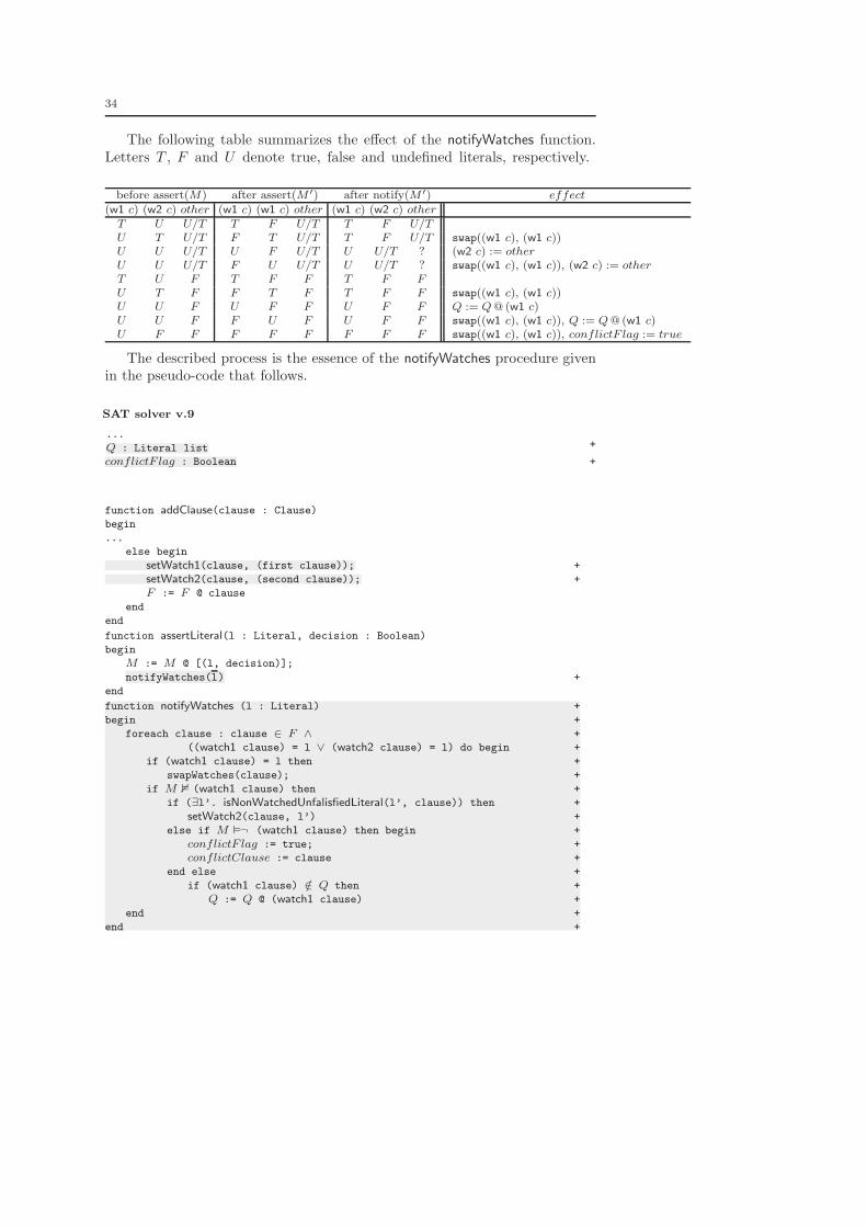
The following table summarizes the effect of the notifyWatches function.Letters T , F and U denote true, false and undefined literals, respectively.

before assert(M) after assert(M ′) after notify(M ′) effect(w1 c) (w2 c) other (w1 c) (w1 c) other (w1 c) (w2 c) other

T U U/T T F U/T T F U/TU T U/T F T U/T T F U/T swap((w1 c), (w1 c))U U U/T U F U/T U U/T ? (w2 c) := otherU U U/T F U U/T U U/T ? swap((w1 c), (w1 c)), (w2 c) := otherT U F T F F T F FU T F F T F T F F swap((w1 c), (w1 c))U U F U F F U F F Q := Q @ (w1 c)U U F F U F U F F swap((w1 c), (w1 c)), Q := Q @ (w1 c)U F F F F F F F F swap((w1 c), (w1 c)), conflictF lag := true

The described process is the essence of the notifyWatches procedure givenin the pseudo-code that follows.

SAT solver v.9

...

Q : Literal list +

conflictF lag : Boolean +

function addClause(clause : Clause)

begin

...

else begin

setWatch1(clause, (first clause)); +

setWatch2(clause, (second clause)); +

F := F @ clause

end

end

function assertLiteral(l : Literal, decision : Boolean)

begin

M := M @ [(l, decision)];

notifyWatches(l) +

end

function notifyWatches (l : Literal) +

begin +

foreach clause : clause ∈ F ∧ +

((watch1 clause) = l ∨ (watch2 clause) = l) do begin +

if (watch1 clause) = l then +

swapWatches(clause); +

if M 2 (watch1 clause) then +

if (∃l’. isNonWatchedUnfalisfiedLiteral(l’, clause)) then +

setWatch2(clause, l’) +

else if M �¬ (watch1 clause) then begin +

conflictF lag := true; +

conflictClause := clause +

end else +

if (watch1 clause) /∈ Q then +

Q := Q @ (watch1 clause) +

end +

end +

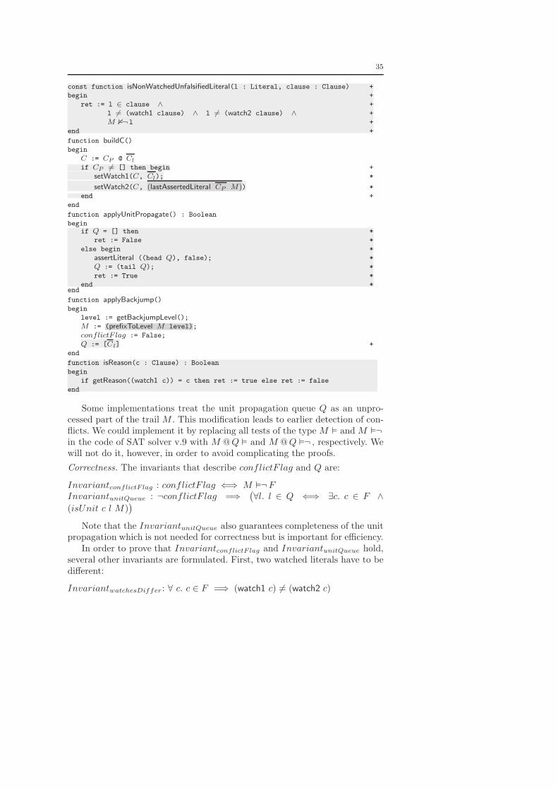
35

const function isNonWatchedUnfalsifiedLiteral(l : Literal, clause : Clause) +

begin +

ret := l ∈ clause ∧ +

l 6= (watch1 clause) ∧ l 6= (watch2 clause) ∧ +

M 2¬ l +

end +

function buildC()begin

C := CP @ Cl

if CP 6= [] then begin +

setWatch1(C, Cl); *

setWatch2(C, (lastAssertedLiteral CP M)) *

end +

end

function applyUnitPropagate() : Boolean

beginif Q = [] then *

ret := False *

else begin *

assertLiteral ((head Q), false); *

Q := (tail Q); *

ret := True *

end *end

function applyBackjump()begin

level := getBackjumpLevel();M := (prefixToLevel M level);

conflictF lag := False;

Q := [Cl] +

end

function isReason(c : Clause) : Boolean

begin

if getReason((watch1 c)) = c then ret := true else ret := false

end

Some implementations treat the unit propagation queue Q as an unpro-cessed part of the trail M . This modification leads to earlier detection of con-flicts. We could implement it by replacing all tests of the type M � and M �¬in the code of SAT solver v.9 with M @ Q � and M @ Q �¬ , respectively. Wewill not do it, however, in order to avoid complicating the proofs.

Correctness. The invariants that describe conflictF lag and Q are:

InvariantconflictF lag : conflictF lag ⇐⇒ M �¬FInvariantunitQueue : ¬conflictF lag =⇒

(

∀l. l ∈ Q ⇐⇒ ∃c. c ∈ F ∧

(isUnit c l M))

Note that the InvariantunitQueue also guarantees completeness of the unitpropagation which is not needed for correctness but is important for efficiency.

In order to prove that InvariantconflictF lag and InvariantunitQueue hold,several other invariants are formulated. First, two watched literals have to bedifferent:

InvariantwatchesDiffer : ∀ c. c ∈ F =⇒ (watch1 c) 6= (watch2 c)

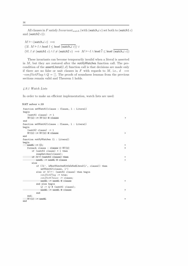
36

All clauses in F satisfy Invariantwatch (with (watch i c) set both to (watch1 c)and (watch2 c)):

M �¬ (watch i c) =⇒

(∃l. M � l ∧ level l ≤ level (watch i c)) ∨

(∀l. l 6= (watch1 c) ∧ l 6= (watch2 c) =⇒ M �¬ l ∧ level l ≤ level (watch i c))

These invariants can become temporarily invalid when a literal is assertedin M , but they are restored after the notifyWatches function call. The pre-condition of the assertLiteral(l, d) function call is that decisions are made onlyif there are no false or unit clauses in F with regards to M , i.e., d =⇒¬conflictF lag ∧ Q = [ ]. The proofs of soundness lemmas from the previoussections remain valid and Theorem 1 holds.

4.9.1 Watch Lists

In order to make an efficient implementation, watch lists are used:

SAT solver v.10

function setWatch1(clause : Clause, l : Literal)

begin

(watch1 clause) := l

W(l) := W(l) @ clause +

end

function setWatch2(clause : Clause, l : Literal)

begin

(watch2 clause) := l

W(l) := W(l) @ clause +

end

function notifyWatches (l : Literal)

beginnewWL := []; +

foreach clause : clause ∈ W(l) *

if (watch1 clause) = l then

swapWatches(clause);

if M � (watch1 clause) then +

newWL := newWL @ clause +

else

if (∃l’. isNonWatchedUnfalisfiedLiteral(l’, clause)) then

setWatch2(clause, l’)

else if M �¬ (watch1 clause) then begin

conflictF lag := true;

conflictClause := clause;

newWL := newWL @ clause +

end else begin

Q := Q @ (watch1 clause);

newWL := newWL @ clause +

end

end;

W(l) := newWL +end

37

function removeClause(c : Clause)

begin

W ((watch1 c)) := W ((watch1 c)) \ c; *

W ((watch2 c)) := W ((watch2 c)) \ c *

end

When a literal stops being watched, its watch list must be updated, andthe corresponding clause should be removed from the list. In one notifyWatches

function call, this list is traversed and many such remove operations can hap-pen. It turns out that it is more efficient to regenerate the watch list of thefalsified literal, than to perform these remove operations, so the clauses forwhich this watch did not change, are reinserted in the watch list newWl. Thislooks as a strange solution, but is in fact an important feature. Being the heartof boolean constraint propagation, the notifyWatches function is crucial for thesolver’s efficiency, because the solver can spend up to 80% of time in it [ES04].

Correctness. Invariant that describes watch lists is:

InvariantwatchLists : c ∈ W (l) ⇔ c ∈ F ∧ ((watch1 c) = l ∨ (watch2 c) = l)

5 Related work

Detailed surveys of SAT solver development can be found in [GKSS07,ZM02,BHZ06]. There is about forty-five years of research invested in DPLL-basedSAT solvers. Earlier SAT solvers based on DPLL include Tableau (NTAB),POSIT, 2cl and CSAT, among others[GKSS07]. In the last fifteen years, therehas been a significant growth and success in SAT solver research based on theDPLL framework. Many practical applications emerged, which pushed thesesolvers to their limits and provided strong motivation for finding even moreefficient algorithms. In the mid 1990’s, this led to a new generation of solverssuch as SATO [Zha97], Chaff [MMZ+01], and BerkMin [GN02] which pay alot of attention to optimizing various aspects of the DPLL algorithm. AnnualSAT competitions have led to the development of dozens of clever implemen-tations of such solvers, exploration of many new techniques, and the creationof an extensive suite of real-world instances as well as challenging hand-craftedbenchmark problems. Some of the most successful DPLL-based solvers in re-cent competitions are Rsat [PD07], Picosat[Bie08], Minisat [ES04], Tinisat[Hua07a], etc. SAT4J is a solver implemented in JAVA in which attention hasbeen put on the code design.

Non-chronological backtracking (conflict-directed backjumping), was pro-posed first in the Constraint Satisfaction Problem (CSP) domain [BHZ06].This, together with conflict-driven learning were first incorporated into a SATsolver in the mid 1990’s by Silva and Sakallah in GRASP [MSS99], and byBayardo and Schrag in rel_sat [BS97]. Conflict clause minimization was in-troduced by Een and Sorensson [ES04] in their solver Minisat. Randomizedrestarts were introduced by Gomes et al. [GSK98] and further developed byBaptista and Marques-Silva [BMS00]. The watch literals scheme by Moskewicz

38

et al. was introduced in their solver zChaff [MMZ+01], and is now a standardmethod used by most SAT solvers for efficient constraint propagation.

The first correctness proof of DPLL with clause learning is given in [ZM03].The given proof is informal and omits a lot of important details. Formal de-scriptions of SAT solvers in a form of state-transition systems were givenin [NOT06,KG07], together with descriptions of related SMT Solvers. Thesepapers contain correctness proof, although presented systems hide many im-portant implementation aspects.

6 Conclusions

In this paper we have developed the core of SAT solver implementation basedon a modified DPLL algorithm. We tried to make a clean separation betweendifferent concepts, and all techniques, algorithms, and data-structures were in-troduced one-by-one, in separate sections. The code follows higher level solverdescriptions [KG07] and is, in our opinion, easier to understand, modify andreason about than the code available in existing presentations (e.g., [ES04]).Heuristic components of the solver were not investigated. We hope that thismethodological approach makes this paper usable as a tutorial and that itcould significantly help interested reader in understanding and learning de-tails of modern SAT solver implementation, especially to researchers that arenew to this field. The solver descriptions, although given in pseudo-code, couldbe converted to a real programming language implementation.

The main part of the paper also provides conditions that have to be provedto ensure solver’s partial correctness. Proofs of correctness conditions are avail-able in the extended version of this paper and original Isabelle proof documents[Mar08]. To the best of our knowledge, this paper gives the first formalizationand correctness proof for some low-level implementation techniques, most no-tably the two-watch literal scheme. We hope that these proofs could help inbetter understanding what conditions are sufficient for solver correctness. Forexample, in [NOT06] the paper [ZM03] is criticized for claiming that the newdecisions should not be made in the presence of conflict or unit clauses. Fromour formalization, it is clear that this is an important invariant of the two-watch literal propagation scheme, and that, although it need not hold for themore abstract rule-based system, it has to hold to ensure the correctness if thetwo-watch literal propagation is used.

Acknowledgements The author would like to thank Dr. Predrag Janicic and anonymousreviewers for carefully reading the manuscript and giving valuable suggestions and advices.

References

[Bar03] C. Barrett. Checking validity of quantifier-free formulas in combinations offirst-order theories. In Ph.D. thesis, Stanford University, 2003.

[Bie08] A. Biere. PicoSAT essentials. In JSAT, vol. 4, pp. 75-97, 2008.

39

[BHZ06] L. Bordeaux, Y. Hamadi, and L. Zhang. Propositional satisfiability and con-straint programming: A comparative survey. In ACM Surveys, 2006.

[BKS04] P. Beame, H. Kautz, and A. Sabharwal. Towards understanding and harnessingthe potential of clause learning. J. Artif. Intell. Res. (JAIR), 22:319–351, 2004.

[BMS00] L. Baptista and J. P. Marques-Silva. Using randomization and learning to solvehard real-world instances of satisfiability. In 6th CP, Singapore, 2000.

[BS97] R. J. Jr. Bayardo and R. C. Schrag. Using CSP look-back techniques to solvereal-world SAT instances. In 14th AAAI, pp. 203–208, Providence, USA, 1997.

[Coo71] S. A. Cook. The complexity of theorem-proving procedures. In 3rd STOC, pp.151–158, New York, USA, 1971.

[DLL62] M. Davis, G. Logemann, and D. Loveland. A machine program for theorem-proving. Commun. ACM, 5(7):394–397, 1962.

[DP60] M. Davis and H. Putnam. A computing procedure for quantification theory. J.ACM, 7(3):201–215, 1960.

[ES04] N. Een and N. Sorensson. An extensible SAT solver. Theory and Applicationsof Satisfiability Testing. pp. 502–518. 2004.

[GKSS07] C P. Gomes, H. Kautz, A. Sabharwal, and B. Selman. Satisfiability solvers. InHandbook of Knowledge Representation. Elsevier, 2007. to appear.

[GN02] E. Goldberg and Y. Novikov. Berkmin: A fast and robust SAT solver, DesignAutomation and Test in Europe (DATE), pp. 142–149, 2002.

[GSK98] C. Gomes, B. Selman, and H. Kautz. Boosting combinatorial search throughrandomization. In 15th AAAI, pp. 431–437, Madison, WI, USA, 1998.

[Hoa69] C. A. R. Hoare. An axiomatic basis for computer programming. Commun.ACM, 12(10):576–580, 1969.

[Hua07a] J. Huang. A case for simple SAT solvers. In CP, pp. 839–846, 2007.[Hua07b] J. Huang. The effect of restarts on the efficiency of clause learning. In IJCAI,

pp. 2318–2323, 2007.[KG07] S. Krstic and A. Goel. Architecting solvers for SAT modulo theories: Nelson-

Oppen with DPLL. In FroCos, pp. 1–27, 2007.[Mar08] F. Maric, SAT solver verification. The Archive of Formal Proofs, http://afp.

sf.net/entries/SATSolverVerification.shtml.[MMZ+01] M. W. Moskewicz, C. F. Madigan, Y. Zhao, L. Zhang, and S. Malik. Chaff:

Engineering an efficient SAT solver. In 38th DAC, 2001.[MS99] J. P. Marques-Silva. The impact of branching heuristics in propositional satis-

fiability algorithms. In EPIA ’99, pp. 62–74, London, UK, 1999.[MSS99] J P. Marques-Silva and K A. Sakallah. Grasp: A search algorithm for proposi-

tional satisfiability. IEEE Transactions on Computers, 48(5):506–521, 1999.[NOT06] R. Nieuwenhuis, A. Oliveras, and C. Tinelli. Solving SAT and SAT Mod-

ulo Theories: from an abstract Davis-Putnam-Logemann-Loveland procedureto DPLL(T). Journal of the ACM, 53(6):937–977, 2006.

[NPW02] T. Nipkow, L. C. Paulson, and M. Wenzel. Isabelle/HOL — A proof assistantfor Higher-Order Logic, volume 2283 of LNCS. Springer, 2002.

[PD07] K. Pipatsrisawat and A. Darwiche. A lightweight component caching schemefor satisfiability solvers. In SAT, pp. 294–299, 2007.

[SS96] J. P. Marques Silva and K. A. Sakallah. Conflict analysis in search algorithmsfor satisfiability. In 8th ICTAI, pp. 467, Washington DC, USA, 1996.

[Wie03] F. Wiedijk. Comparing mathematical provers. In MKM03, pp. 188–202, volume2594 of LNCS, 2003.

[Zha97] H. Zhang. SATO: An efficient propositional prover. In CADE-14, pp. 272–275,London, UK, 1997.

[ZM02] L. Zhang and S. Malik. The quest for efficient boolean satisfiability solvers. In14th CAV, pp. 17–36, London, UK, 2002.

[ZM03] L. Zhang and S. Malik. Validating SAT solvers using independent resolution-based checker. In DATE’03, pp. 10880, Washington DC, USA, 2003.

[ZMMM01] L. Zhang, C. F. Madigan, M. H. Moskewicz, and S. Malik. Efficient conflictdriven learning in a boolean satisfiability solver. In ICCAD ’01, pp. 279–285,Piscataway, NJ, USA, 2001.