~l

M I N I S T R Y . OF A V I A T I O N

R. & M. No. 3217

A E R O N A U T I C A L RESEARCH C O U N C I L

REPORTS AND MEMORANDA

Formulae for Calculating the Camber Surfaces of Thin Swept-Back Wings of Arbitrary Plan-form

with Subsonic Leading Edges, and Specified .Load Distribution

By G. M . ROPER, M . A . , P h . D .

: - % - . . ' , ' , . ,, : , "., :

L O N D O N : HER MAJESTY'S S T A T I O N E R Y O F F I C E

1961

- PRIC~.: l ls . 6d. N~.T

Formulae for Calculating the Camber Surfaces of Thin Swept-Back Wings of Arbitrary Plan-form

with Subsonic Leading Edges, and Specified Load Distribution

B y G. M. ROPER, M.A., Ph.D.

COMMUNICATED BY THE DEPUTY CONTROLLER AIRCRAFT (RESEARCH AND DEVELOPMENT), MINISTRY OF AVIATION

Reports and Memoranda No. 32-r7"

June, ~959

Summary. Formulae for calculating the-gradients and ordinates of the camber surfaces of swept-back wings of arbitrary plan-form with subsonic leading edges, and specified load distribution, are given, including those which have been programmed and used for DEUCE calculations for some swept-back and M-wings with curved leading edges.

Some methods for the numerical calculation of singular integrals are given. For polygonal wings with simple load distributions, the equation of the camber surface is given in closed

form. This is useful for obtaining approximate results for more general plan-forms.

1. Introduction. This paper is a brief account of a method for calculating the gradients and ordinates of thin swept-back wings of arbitrary plan-form, with subsonic leading edges. No claim is made that anything is new except perhaps the suggested treatment of singularities for numerical

integration, and some of the formulae and integrations produced. Integrals, based on linearised supersonic theory, for calculating the upwash or the streamwise

gradients of a wing surface for a given load distribution (the direct problem--Ref. 3) have been known for some time. But until fairly recently, when large scale calculations with the aid of electronic computers became possible, little use had been made of these integrals for wing design. The need of a method for designing camber surfaces to produce specified load distributions has arisen in connection with a research programme on problems associated with flight at low supersonic

speeds (Refs. 5, 6). In this paper will be found:

(1) the basic integrals and formulae for calculating t ie streamwise gradients and ordinates of a camber surface to support a given load distribution, the wing plan-form being arbitrary, with subsonic leading edges and any trailing edge;

~ Previously issued as R.A.E. Report No. Aero. 2623--A.R.C. 21,430.

(2) formulae for calculating the camber surface for some special forms of load distribution such that a first integration can be performed analytically;

(3) formulae in integral form (which have been programmed and used for calculations on DEUCE) for calculating the camber surface of two particular wings: a swept-back wing and an M-wing, with curved subsonic leading edges and straight subsonic trailing edges;

(4) some approximate formulae, in closed form, for the ordinates of the camber surfaces of wings of arbitrary plan-form with subsonic leading edges and uniform chord loading; (these have been used for some check calculations);

(5) some methods for dealing with singularities. The chief difficulty in programming for the numerical integrations lies in dealing with singularities

which do not exist in real flow, but which arise because of the approximate linear theory used. These singularities are of two kinds:

(1) those which arise because of the mathematical form of the problem. These singularities cannot be avoided and can be dealt with by using the concepts of 'finite part', 'Cauchy principal part', or 'generalised principal part' of an integral in the regions of the singularities before numerical integration is attempted. This method is given in Section 5, and has been used in existing DEUCE programmes;

(2) those which arise from the type of load distribution chosen, such as logarithmic singularities in the gradients at leading or trailing edges, or in gradients and ordinates at centre or 'kink' sections (where the gradient of leading and/or trailing edge is discontinuous). These singularities could be avoided if certain load distributions were chosen (e.g., a loading coefficient of the formf(~, ,7) . (~-F(~?))I/~). But, in practice, the load distributions required seem to be such that some of these singularities must occur.

A method for calculating the ordinates at points on leading or trailing edges, where there are integrable logarithmic singularities, is given in Section 5.

When the load distribution and plan-form are such that logarithmic singularities in both the streamwise gradients and the ordinates occur at centre or kink sections on a wing (due to the fact that the linearised boundary conditions no longer apply), an iteration method could be used to calculate the camber surface near these sections, including both incidence and thickness. Some calculations done for a particular wing showed that convergence could be obtained, but nothing will be written of this here. Some other methods, which have been used for the particular wings mentioned in Section 3 of this R. & M., are given in Refs. 7, 8.

2. Calculation of the Shape of the Camber Surface of a Wing of Given Plan-form for a Given Load Distribution. Considering incidence effects only, and using the linear small perturbation theory of supersonic flow, Volterra (Ref. 1) has shown that the acceleration potential f~ can be expressed in the form

1 a f f A f 2 ( x - ~ ) ( z - C ) d S ~ ( x , y , z ) - 2~ax T [ ( y - ~ ) ~ + ( z - ~ ) ~ ] { ( x - ~ ) ~ ~ [ ( y - ~ ) ~ + ( - )]} - z 11 , ( 1 )

where f~ = V ~x' V is the free stream velocity, parallel to the x-axis, x, y, z are a right-handed

system of rectangular Cartesian co-ordinates, z being measured upwards, and ¢ is the perturbation velocity potential. M is the free stream Mach number and/?~ = M 2 - 1. Af~ is the jump in the value of f~ across the surface of the wing, and integration is over the part, ~, of the wing surface for which ( x - ~)~ - fl~ [ ( y - ~)~ + ( z - ~)~] > 0 and x - ~ > O.

2

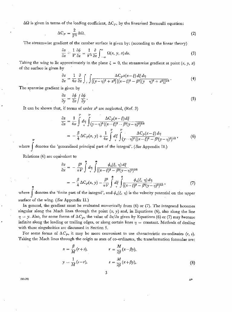
Af2 is given in terms of the loading coefficient, ACe, by the linearised Bernoulli equation:

ACe = 2 A~. (2)

The streamwise gradient of the camber surface is given by: (according to the linear theory)

8z~_ 1 8 y, (3)

Ox V 8z V 2 8z ~o

Taking the wing to lie approximately in the plane ~ = 0, the streamwise gradient at point (x, y, z) of the surface is given by

8 z _ l 8 8x 4~ 8z

The spanwise gradient is given by

f f ACez(x - ~) d(&7 r [(Y-- ~7) z + Z~] [(X-- ~)2 _ / ~ 2 { ( y _ ~7)2 + z2}]112 " (4)

az s~ / 0¢ a y - az / ay (5)

It can be shown that, if terms of order z 2 are neglected, (Ref. 3)

P P

8z 1 f A C e ( x - ~) d~

P P

p - 4 AC~(x, y) + ~ d? ( _ , )2{~S_~-Z-~3~_~)2}1/2, (6)

where j denotes the 'generalised principal part of the integral'. (see Appendix II.)

Relations (6) are equivalent to

_ ( ~u(~, ~)d~

~,(~, 7) dv

where [- denotes the 'finite part of the integral', and ~u(~, ~7) is the velocity potential on the upper

surface of the wing. (See Appendix II.) In general, the gradient must be evaluated numerically from (6) or (7). The integrand becomes

singular along the Mach lines through the point (x, y) and, in Equations (6), also along the line ~/ = y. Also, for some forms of ACe, the value of Oz/ax given by Equations (6) or (7) may become infinite along the leading or trailing edges, or along certain lines ~7 = constant. Methods of dealing with these singularities are discussed in Section 5.

For some forms of ACe, it may be more convenient to use characteristic co-ordinates (r, s). Taking the Mach lines through the origin as axes of co-ordinates, the transformation formulae are:

(8)

-tiM M x = (r + s), ," = ~ ( x - flY),

1 M y = ~ ( s - r), s = yfi (x + fly),

(82476) A*

and the formula for the streamwise gradient is

P P

0,%' -- 4~ {3 -- 31 -- Y -- 1"1} 2 { ( Y - y l ) ( S - $ 1 ) } 112' (9)

M M where r, = ~ (~:-]3~), . . = ~ (~:+/3~1), and the region of integration r is that part of the wing

plan-form for which r - q > 0 and s - s 1 > 0. Relation (9) is equivalent to

a ~ _ M ( (¢~(q,*l)dr ld ,1 ( lo)

ax 4~ v J~ J{(r - ,1) (s - $1)}~ ~'

(which can also be put into other forms).

The ordinates z of the camber surface are found by numerical integration from

z = E & +f (y ) , (11)

where f ( y ) is a small arbitrary function of y , or

?x Oz z - z o = ! - - d x , (12)

J~o 0x

where, for each value of y, z 0 and x 0 are arbitrary constants.

I f ACp is chosen so that a first integration wi th respect to ~ or ~7 can be performed analytically,

Oz/Ox can be found by numerical integration with respect to a single variable (~/or ~).

Some special forms of ACp are discussed below. (The y-axis is taken through the foremost point,

or points, of the leading edge.)

(1) I f Ac~ = Ho(~) + E K~H,~(~)], (13)

where Ho(~?), H~(V ) are functions of ~ only, and n is a positive integer, P P

az 1 ~. Ho(~) Xo, laT + X~, ~ d~ , Ox - 4re ',1 (Y - ~7)~ ~ " ~1 (Y - ~)~

where

1 ( '2(~1, (X-- ~) d~ ~2 I _ {(/~ __ ~)2}1]2 Xo = = _ ~)2 _/32(y (15a) ' j~l(,/) {(X -- ~ ~ ~2~y-__ ~)2}1i9~ gl t-

X . I = (~2,,) ~ " ( x - ~ ) d ~ , (15b)

T h e limits of integration are given by:

~(~) = f(~);

~z(r/) = x - / 3 [y - , [ ~< g(w), x - f(~?) >/9 lY - ~7 [

or ~2(~/) = g(~?) ~< x - 19 [ y - ~7 1;

~1 = ~ = 0 for x - f (~?) </3 ] y - ~ 1, (16)

where ~: = f(~l), ~ = g(~?) are the equations of the leading and trailing edge s respectively. ~h, % are given, by the equations

x - f ( . l ) = /~(Y- Vl),

x - f(~/e) = /~(%-y) . (.17)

4

"ql, % are the extreme limits of integration for ~/. Intermediate limits (due to the bounding of the region of integration by other leading or trailing edges) are given by similar equations with the appropriate functions replacing f071), f0%).

Reduction formulae for the calculation of the integrals X~, 1 are given in Appendix I. (2) If

ACv = Go(~:) + £ [rl+G,~(~)], (18)

where Go(es), G~,,(~) are functions of ~ only, and n is a positive integer,

P - 1 F f : Oz 5 A C / x , y ) + Ox 4 G(~:) ( ~ - ~) Yo,~ d~ +

where

P

P

I7o ~ = (,12(~ &7 , j+~+~ (y _ +l)~{(~ _ ~)~ ~ / ~ ( y _ ~)~}1~ =

(19)

+". [ { (x - ~.)2 _ f l 2 ( y _ r/)2}i/2-1 (20a)

• ,~ +,~+<+) ( y _ ~)~{(x_~- ~ ( y _ ~).~}m • (20b)

The limits of integration are given by:

O?"

OY

~*(~) =/-~(¢) > Y /3 '

x - ~ ~1(~) = Y 5 >~ f-l(~:);

~ ( 8 ) = f - l ( ~ ) .< y + _ _ 5

~]2(~) = Y + ~<f -*(~) ;

~<x

71 = ~', = 0 for ¢ > x, (21)

where ~/ = f S ( ~ ) is the equation of the leading edge. (For a yawed wing ~h or % might be a point on a trailing edge.)

Reduction formulae for the calculation of the integrals Y~, 2 are given in Appendix I. (3) Uniform (or variable) chord loading and load varying linearly along the chord:

ACl~ = A - B (chordwise distance from L.E.)

local chord

= A B { ~ - f ( r / ) } g(r/) - f ( r l ) ' (22)

where ~ = f0?), ~ = gO7) are the equations of the leading and trailing edges respectively and A, B are constants (or functions of ~7).

This is a special case of (1) with

- H~(7) - + H(7) = B/{g(7) -f(~7)} and

H0(7) = A + f ( ~ ) . H(7 ) = h(~). (23)

It can be shown that the integrated chord loading is given by

CL(y) = A - ½B, (24),

and hence the total lift coefficient, when A, B are constant is

¢~ = A - ~B. (25)

The chordwise gradient of the camber surface at the point (x, y, z) can be written in the form: (neglecting terms of order z ~)

P

~ z _ / 3 Y~ f F H o ( ~ - x H ( 7 ) sinh ur + ~H(~)(u,.+ ½ sinh 2ur)] d~ ~x - 4-; ~ I [ Y - 7 [

r = 1,2, P

-- Z F(x, y, ~7, zq)d~ - F(x, y, ~7, u2)d~ t - o ~ l a ~1 o

= 2 (G.,b)l - 2 (Gc, a)~; (26)

the summation is over the different regions of integration (cf. Section 3(b) and Fig. 4), and

x - f(v) x - g(~) (27) ul = c o s h - l f i l y _ ~ l , u 2 = c o s h - ~ / 3 l y _ 7 [ ,

~7,, % are given by x -f(~Ta) = /3 [y-7a [, (28) b b

~, ~a are given by x - g(Fc)=/3 [Y- ~ [, (29) d ' d

that is by the points of intersection of the fore Mach lines through the point (x, y) with the leading and trailing edges respectively. The integrands in Equation (26) are of the form

P(x' ~){(x-~)~ - /3Z(Y-~'l)~}l/2 ~ l x - ~ l (30) ( y _ ~)~ + H(~) cosh-~ /3 ~ - - 7 I '

where ~ = f(~7) or g(7), and P(x, 7) is a function of x and 7, and thus become singular along the line 7 = Y in the region of integration.

Methods for dealing with these singularities and those which occur at the leading and trailing edges are given in Section 5.

3. Formulae .for Calculating the Shape of the Camber Surface of Two Particular Swept-back Wings with Uniform (or Variable) Chord Loading, and Load Varying Linearly along the Chord. Formulae for calculating the shape of the camber surface of two particular swept-back wings (see Refs. 5, 6), with load varying linearly along the chord, are given.

For each w i n g : -

The equation of the leading edge is given by ~ = f(7), and the equation of the trailing edge by

T h e loading coefficient is

B(~ - f(w)} (31) A C p = A g(~) - f07 ) '

where A, B are constants. (The formulae given below also apply if A, B are functions of %) All lengths are measured in semi-span lengths. Formulae for calculating the gradient, 3z/3x, for two swept-back wings, are given below. The

ordinate, z, is calculated from Equation (11) or (12).

(a) Swept-back wing with partly curved subsonic leading edges and straight subsonic trailing edges (Fig. 1):

The plan-form of the wing is given by

o ~<. I~1 ~< ½, f07) = k 1~7 l; } ~<~ Iwl<-a,f(w)=kl~I+c[1-{2(1-lwl)}~¢V;, g(7) = c + k l T I . (32)

The length of the root chord is c and the leading edge sweep-back angle is tan-lk. T he streamwise gradient of the camber surface at the point (x, y, z) is given by (y > 0)

P

0z /3 f~z rh (~ / ) - all(*?)sinh u l + ~ H(~7)(ul+ ½ sinh 2ut) 1 d~

P

f ~2F(x, u O d ~ = (G~,~)I, i f x /3y~< Y, C; (33)

and '

3x ( G , , ) , - ( G , & , i f x - & ~> c, (34)

where H(~/) = B/(g(~) - / (~ / ) } , h07 ) = A + f ( 7 ) . H(~). T he variables u r and the limits ~r are given by

- f ( ~ ) x - g (~ ) . (35) gl = c°sh-1/3 [ y _ V [, u2 = cosh -1/3 l Y - ~/[ '

x - f ( 7 0 = /3(Y-~h), x - f (~ /~ ) = / 3 ( ~ z - y ) ,

x - g(~3) = /3(y - ~3), x - g074) = / 3 ( y - ~7,), (36)

71, 73 being < 0 and ~z, 74 > 0.

(b) T h e N-wing (Fig. 3): The plan-form of the wing is given by

o ~ I~l ~< ~, f (7) = k l (½- 17 I), gO7) = cl + k~(½- ]-q I);

{ ~< 171 ~< 1, f (7 ) = k( [~71 - 1 ) + c1[1 - {2 (1 - [7 1)}1/2]z,

g(7) = c~ + k ( 1 7 1 - ½ ) . (37)

T h e leading edges are swept forward at an angle tan -1 hi (for 0 ~< I ~7 [ ~< ½) and swept-back at angle tan- l f ' (~)(½ ~ 171 ~< 1); and the trailing edges swept-back at angles tan- lk2(0 ~< 1~TI < ½) and tan-~k(½ ~< 171 ~ 1). T h e length of the 'kink' chord (at Iwl -- ½) is c~, and is such that c~ + k /2 <

3/3/2 (so that the wing tips at 7 = + 1 and 7 = - 1 are outside the Mach lines from the leading edge tips at ~7 = - ½, ~ = + ½ respectively). T h e length of the root chord is c.

The streamwise gradient of the camber surface at the point (x, y, z) is of the form (y > 0)

where

P OZ [~lb Ox ~ ., .,1. F ( . , y , ~, .r) dr - 2: ( a . , 0,,

x - f (v) x - g(~7) ' u, = cosh-*/3 [ y - ~ l ' u2 = cosh-*/3 lY- n 1'

and f(~7), g(7/) are given by (37).

r = l o r 2

(38)

(39)

0 < y < ½

3. x - 5Y 4 ½fi, x -~ 5Y ~ C, -Jr- ½5 (G,, 2),

4. ~ - 5y <. ½-5, x + 50, >1 q + ½5 (0 , ,2) , - (c~,~)2

5. ½k, > x - 5y > ~5, x + 5y <. c, + ½5 (G,, 2), + (G~, &

6. ½k, > x - 53, >>- ½5, * + 5y > c~ + ½5 ( c , , 2), + (c~, o), - (%, , )2

7. x - fly <<. ½1q, x + fly <~ q + ½5 (Ga, 2)x

8. ½k, <. x - 5y <- ~, + ½5, x + 5y > c~ + ½5 ( % , 2), - (G~, &

9. c + ½k, > x - / 3 y > c, + ½5 (Gs, 2), - (Ga, 4)2 - (G7, 8)2

% (r = 1, 2, . . . 8) are given by the equations

x - f ( ~ b ) = 51y-~l,

1. x - 5 y < q - ½5 (G, , 2),

2. x - 5 y > q - ½/3 (G, .2 ) , - ( G 3 , &

x - g(n~) = 5 l y - n,. I,

r = 1,6 (0~< I rl ~½)

r = 2 , 5 (½.< Intl.<l) r = 3 , S (0.< ln~l.<½) r = 4 , 7 (½4 1%!~<1) (40)

The formulae given above for calculating the camber surface of wings (a), (b) have been

programmed and used for calculations on a D E U C E computer.

4. Approximate Formulae for the Calculation of the Ordinates of the Camber Surfaces of Wings with Subsonic .Leading Edges and Subsonic or Supersonic Trailing Edges, with Uniform Chord Loading. An approximate method for the calculation of the ordinates of the camber surface of a wing of any plan-form with subsonic leading edges and any trailing edge is suggested, whereby curved leading and trailing edges are approximated by polygons. I t is also useful in some cases to use an approximate formula for the prescribed load distribution, so that formulae for the gradients and ordinates at points on the wing can be obtained in closed form.

Region 0~[~

½ < y < l

The formulae for calculating az/Ox in the different regions of the wing are given below: (see Figs. 3, 4)

The formulae can be used for calculations on a desk machine or for Interpretive Scheme calcula- tions on a D E U C E computer. This method was used for some preliminary calculations for both the swept-back wing and the M-wing mentioned in Section 3; these served as a partial check on the D E U C E calculations for which the integrals given in that section were programmed.

The resulting approximate formulae for any wing with prescribed uniform chord loading are given below. Similar formulae could be derived for other loadings.

Using the notation of Section 3, the loading coefficient is

A C p = A B(~- f (~?)) (41) local chord '

where A and B are Constants. The vertices of the approximating leading-edge and trailing-edge polygons are on the edges at

points y = yr (r = 0, 1, 2, . . .), and the slope of a leading or trailing-edge segment is given by

kr = ( X r + l - - xr)/(Y,'+l--Yr), (xr+l > xr), (42 )

:where x,. = f(y~) on a leading edge, and x~ = g(y,.) on a trailing edge. (See Fig. 2.)

The local chord of the segment of the vdng defined by Yr >< Y >< Yr+l is approximated by the average

chord

c~ = ½{g(Yr) + g(Y,.+~) - f(Y,.) - f(Y~+l)}. (43)

[Alternatively, circumscribing polygons could

y = ½(y~+~+yr).] Writing

be taken,

= 3 ( y - y , , ) / ( * - = , , ) ,

[/~r--1-- 1~ ~-12 [1 -1- tg'r~112 e " = \2 ,_1+1] \1 -~%] '

l + P r p,,= ½log l - P , . '

the points of tangency being (say) at

1 u~ = c°sh-1/l'~--~-' (44)

= [A, . - 1'~ 11~ {1 + ~r] 1'~

1 -t- Qr q,. = ½ log [ ~ Q , . , (45)

the formula for the ordinate z at the point (x, y) of the plan-form can be written in the form

= +

fi [ B (x-xr)2R2(t%) 1 , (46)

with xr = f(y~) in the first sum [L], and x r = g(y~) in the second sum [ T]. Rl(tg,.), Rz(~9~) are functions of t% given below. The summation of each sum is for values of r for which both x,. - fiy~ < x - [3y

and x~ + fiy~ < x + fly.

For points (x, y) on the wing plan-form for which x +_ fly <~ g(yr) +_ fly,., or for a wing with all supersonic trailing edges, the second sum [T] does not appear.

The functions R1, R~ are given by

RI(#,) = (a) + (b) (47)

i2(tg'r) = (~' £(-11 )(c)-t- \(}d-))r-1 (e)t 'c/,] (48)

where, for k~ > O, k~_, > O:

(a) = - ()r-/~-1) {//r -- 5/(1 _~,.2)} + (At2_)~_,)~,.u,

(b) -- - 2 V'(A~_~- 1). (1 - h,._~v~,.)p, + 2 ~ / ( a~- 1). (1 - k,~r)qr

(1 -va,2) a!2

) r - - l U r o ' 2 (d) = ( 3 - 2a,_~,) V'(1 -~,Y) - - - 2 - {(217-*- 1)t~,

- 4 1 r _ ~ , . + 2 } + 2 ~- . ~/(~,._~- 1) (1 - ~,_~e,)2pr

( 3 - 2a,e,.) x / (1 =- e,.2) - ~ z { (2~ ,~ - 1)e~ - 4 z & + 2} (e) =

+ 2 ~/(A,. 2 - 1) ] (1 - A,.t~r)Zqr. ( 4 9 )

t (~,.- 1~ '12 (At-I- 1~ 112 When h,. < 0, replace ;~,. by - at, ~/(Ar ~ - 1) by - ~/(Ar ~ - 1), and by , with % + 17 tV~- 17 similar replacements (with suffix r - 1) for k,._ 1 < 0.

A sufficient number of points y~ might be chosen so that the points (x, y) at which the ordinates are to be calculated lie on the middle chords of the segments of the wing. Then

~(y+,+I-yD = 1 - l - Y ~(Yr Y~+l), and ~ - 2(x- xD

Also the approximation to the local chord might be taken as

If point (x, y) lies on a leading-edge or trailing-edge segment of slope + k;, va~. = ur = cosh-15,., and the last terms in (b) and (e), [(1 - Z~)q~, (1 - ~r)2q,.], tend to zero.

(Point (xr, y,.) on an edge would be taken as a point on segment of slope hr_~. )

___ l /x , ,

If )t,._ 1 = A,. and cr_ 1 g= c~:

and (a) = (b) = O; (e) = (d),

Rl(e,.) = 0; R~(eD = ~,. c(_1 ( ( c ) - ( d ) ) .

10

where

If Ar_l.= - 2~ and cr_ 1 = c~

(a) = - 2 ~ {u~ - ~/(1-t9~2)}

(b)

(1 c!_1) (c)

R#3

= 2 V ( ~ ~- l) (~ , - ~a,~)

= 0

= 2 [ - A~{u~ - a / ( 1 - t%2)) + ~ ( ~ 2 _ 1)(v~- ?@,.w~)]

[~i~ 3~ ~ / ( l _ ~ ~) 2 {2 + (2X~ ~ - 1)t% ~} -~-

+ V'(~,Y- 1) {2,~,3~w~ - (1 +,~2~%2)v~} 1 A

(50)

(51)

l+Z~ l+W~l v~ = ½ log Vz-v; ' ~o~ = ½ log ~ ;

a~ . V ( I _ ~ ) , w~- ~/(1-~) •

When point (x, y) lies on the leading or trailing-edge segment (slope kr), (50), (51) become

R~(t%) = 2 {V'(A, 2 - 1) - A~ c o s h - ~ }

R2(~5~ ) = 1 [(4A~ 2 - 1) ] Cr [ . ~ r r c°sh-~Ar- 3~¢/(~2--1)

(52)

(53)

For the swept-back wing (Figs. 1, 2) for which g(~) = c + k ]7 I and, for 0 < ~ ~< ½, f (~) = h ]~ ], for all points (x, y) on the wing such that x + py 4 ½(k+p), (i.e., all points upstream of the after Mach lines from leading-edge points y = + ½) the exact solution of the linearised equation is

obtained from (46) with (50)-(53) by putting r = 0, x 0 = Y0 = 0, Yl = ½, k,. = k = - k ~ _ l in

sum ILl when x + fly < c, and in both sums [L], [7"] when x + fly > c.

I t is not suggested that it would be better to use approximate formulae than to use the integral forms, except perhaps for parts of the wing where the approximate formulae become exact. The above formulae were used to obtain some preliminary results fairly quickly before a D E U C E programme had been made. They were also found useful later for checking.

5. The Numerical Evaluation of some Singular Integrals. Analytical methods for evaluating the 'finite part ' of an integral, the 'Cauchy principal part ' and the 'generalised principal part ' of an integral are well known (see Refs. 3, 4 for example) and details will not be given here. For purposes of reference, definitions and relevant formulae are given in Appendix II.

For the integrals in Equation (7) in Section 2, one of the usual methods for evaluating the finite part of an integral can be used (see Appendix II). Equations (6) are derived from (7) by an integration by parts and evaluation of the finite part.

Integrals discussed here are those which arise from Equations (6): (1) when integration with respect to ~ is performed analytically; (2) when integration with respect to ~/is performed analytically; (3) when the double integral is evaluated numerically; (4) when po!nt (x, y) is on a leading or trailing edge.

11

(1) I f ACp(~, 7) is of such a fo rm that a first integration wi th respect to ~ can be per formed

analytically, in general, integrals of the fo rm

o r

P

f ~'~ P(~ , 7) { ( ~ - F (7 ) ) ~ - ~ ( Y - 7 )~F ~ ,11 (y _ 7) ~ d7

P

~'~ P(x, 7) cosh-X x - F(7 ) d7

have to be evaluated numerically. ~ = F(7 ) is the equation of a leading or trailing edge, and the

functions P(x, 7), F(7) are continuous in the range 7t ~< ~? ~ 72.

For the numerical evaluation of these integrals when 7~ < Y < 72, w r i t e

P P

? f ° r ; = + + , ~ll ~ql d b a

where a, b are suitably chosen, and 71 < a < y < b < 72. ( I t is usually not convenient to take a = 71

or b = 7~, one reason being that the integrand may diverge for a different reason near 7 = 71 or 72.)

T h e integrands in the first and second integrals are finite and cause no difficulty. T h e third integral

can be put in the form

P

d7

1 1 P(x, b) . R(~, y , b) - - - - - P(x, a) . R(~, y , ~)

b - y y - a

b - y + [P'(x, y) ( x - F(y)) - P(x, y) . F'(y)] log - - - y - a fo P(x, 3~ n) d7

. R(~, y , 7)

f ~ P'(x, 7). R(x, y, 7) - P'(x, y)(x-F(y)) d7 a Y - 7

+ fb IP(x, n)(x-F(n))F'(n) R(x, y, 7)

7 1 - P(~ , y ) . F ' ( ~ ) / dT, (54)

" - / Y - - 7

where R(x, y, 7) -- { ( x - F ( 7 ) ) ~ - fi2(y_ 7)e}v~, and the dash indicates differentiation with respect

to 7 or y.

T h e integrands of the three integrals in (54) are finite at 7 = Y provided that P(x, ~7) and P'(x, 7) exist and are single-valued at 7 = Y. A formula similar to (54) has been used in a D E U C E programme.

Another fo rm (useful if the expansion converges sufficiently rapidly near 7 = Y) can be obtained

by expanding R(x, y, 7) as a power series in ( y - ,/). T h u s

P

f b p(~, 7). R(~, y, 7) d7

P

- . ( y - 7) ~ ~ ( x - F (7 ) ) ~ - g ( x - F (7 ) ) ' - " (55)

12

The first integral

P ,~b P(x, ~ ) ( x - F ( ~ ) )

3o (y- v)~ is equal to

Pl(x, b)

b - y

P

f b p1(x ' 7) .

Pl(x, a) b - y - - + P~'(x, y ) log y - a y a

( ~ P~'(x, ~1) - PI'( x, Y) &7. .I Y ~7 (56)

f b cosh -~ x - F(*/) P(x, 7) d~7 o

= ( b - y ) P ( x , b) cosh -~ x - F(b) 5(b-y)

f P(~, 7) [~- F(~) - F'(~)(y- ~)] + . R ( x , y , 7)

d~

+ f f P'(x, n)(Y-V)cosh-l ~ y F ~ I dv,

in which the integrands are finite at ~/ = y.

(2) If a first integration with respect to ~/is possible by analytical methods, integrals of the form

P

f x Q(x, y, ~) d~ o 3 - - ?

occur, the function Q(x, y, ~) being continuous in the range 0 ~< ~ ~< x, and generally (but not

always) of such a form that the integral converges near ~ = x. The treatment of this integral depends on the particular forms of ACp(~:, ~1) and F(~?).

(3) If the double integral in Equation (6) is evaluated n u me r i c a l l y : - The double integral to be evaluated is

P P

r (Y-- n)2{( x - ~)~ -- t~2(Y-- rl)~} 1t2'

where the region of integration, r, is the region on the wing plan-form for which x - ~ 1> fi lY- ~ l" This integral can be written in the form

P

P P {(~-

13

- - + ( y - a ) P ( x , a ) c o s h -1 - -

(82476) B

x-F(a) ~(y-a)

(57)

integral in the form

P

The integrands in (56) and the remaining terms of the series in (55) are finite or zero at ~7 = Y- The numerical evaluation of the integral

P

f b cosh -1 x - F07 )

is fairly simple (provided that ACp and Fi~ ) are suitably chosen). One method is to write the

~1 = f (v ) and ~ = x - fl [ y - ~2 [ or g(v), and the first integral is of the form

P

f ~ dn, w < Y < ~2, P(x, Y, ~1) . R(x, Y, ~)

~ (Y - ~)~

the same form as given in (54) and (55). The integrand of the second integral in (58) is finite in the region of integration except near

r] = y, (ACp(~, .q) being suitably chosen). For integration over a strip a <~ ~7 <<. b, the integral

could be writ ten in the form

l y - v l

I{(x-~)2 - [32(Y-~7)2}aI2 ~i ACp( ~, ~) - ( x -~ ) ~ A Cp(~, ~7) 1 (y _ ~)~ d~ &

, (e ) - d~ d~, (59)

where ~:1 = f (a) or f (b ) (whichever is least), and in the second integral a(~), b(~) vary over part of the range ~1 ~< ~'~ x for which the integral is to be evaluated. Before numerical evaluation, the second integral in (59) should be put in a form similar to that given in (54).

(4) When the point (x, y) is on a leading or trailing edge (Equation: ~ = F(~))), x = F(y) and

~1 or % is equal to y; ~1, ~2 are given by

Integrals of the form

P

x - F(nr) = 5 I s - I r = 1,2.

f ~2 P(x, ~) cosh -1 x - F(~7) d~/ ~Jl -~-~

remain finite provided that P(x, ~) is finite in the region of integration. But integrals of the form

P

f ,,2 P(x, ~) {(x - F(~/)) ~ - fi2(y _ 71)2}112

become infinite unless ACt,(~, ~?) is so chosen that

limit P[F(vr), ~] R(x, y, 7) (r = 1 or 2) ~->~,. ( ~ - ~)~

exists. If this limit does not exist, the integral has a logarithmic singularity when ~7, = y, although, in

general, an analytical integration of the singular expression with respect to x is possible (and finite) at x = F(y). This causes some difficulty when numerical methods are used, especially with respect

to the camber shape near the wing tips. Extrapolation near leading and trailing edges has been used in some existing D E U C E programmes.

This is not very satisfactory. A programme for calculating the shape of the surface at the wing tips, where the distances between leading and trailing edges are small is then not possible. It may not even be possible to obtain the shape near the tip' by extrapolation, since the ordinates extrapolated along different lines through the tip may not converge to a unique point there.

14

Some research on methods of programming for such singularities could b e done. One method of dealing with the difficulty is suggested below. (The method is given for an integration with respect to ~7, but a similar method could be used for numerical calculation of the double integral.)

If the point (x, y) is on an edge ~ = F(7), so that the limit % = y, writing

(for small local chord, e.g., near the wing tips, a could be taken equal to 71), the contribution to the ordinate z at point (x, y) from an integral of the form

P

f ,,2 p(x, 7). R(x, y, 7) d7

could be written

where

and

m z = ( m Z ) l -~- ( A z ) ~ ,

; U (AZ) 1 = P(x, 7) { ( x - F(7)) 2 - fi=(y - 7)e} 1'=

(A~)~ = _ {(F'(y))~ -~)~J~ limit *o P(~', y) Q'. y- ~/&'. x---> F ( y ) x

The two integrals in (60) should cause no difficulty, and (61) can be put in the form:

(60)

(61)

( A z h = - {(F'(y))2 - fl2} 1t2 v [log ( y - a) f~°(u ) P(x' , y )dx '

- P(x o, y) (x o - F(y)) log {72(Xo, y) - y}

+ P(x' , y) (x' - F(y)) log (x' - F(72)) Ivfy)

' I1 + P(x' , y) 7 2 - Y "19+F'(7~i dx.' . (62)

It must be remembered that in the integrand, % - 72(x', y), a function of x', y, given by

x ' - F(72) = 5 ( > - Y ) , and that

72(x', y) = y when x' = F(y),

%(x', y) > y when x' > F(y). (63)

The integrand in (62) converges at x' = F(y) and it should be possible to programme (62) for D E U C E , or other electronic computers , and thus avoid the need for extrapolation near the edges and a certain amount of guessing at the wing tips.

15 (82476) B 2

The formula for the total ordinate z at a point (x, y) on an edge would be of the form

z = z o + dx + Z (Az), (64) x0

where Ozl/ax is the contribution to the gradient from other integrals which can be evaluated at the

edge, and x0, z 0 are arbitrary constants or functions of y. A similar formula could be derived if ~/1 = Y.

6. Conclusion. A method has been given for calculating the shapes of camber surfaces of swept-back wings of arbitrary plan-form, with subsonic leading edges and specified load distribution, with particular reference to some of the difficulties encountered in the numerical integrations. The

method is primarily intended for programming for calculations on an automatic digital computer. It is obviously not possible to produce perfectly general formulae or programmes (beyond the basic integrals from which all such formulae would be derived) to suit all plan-forms and all load distributions. The particular methods used must depend partly on the type of load distribution chosen and (to a lesser degree) on the plan-form of the wing.

16

A

A(y, ,7)

a

B

B(y, 7)

b

C(y, 7)

cL(y)

£

C1

F(V)

F(~, y, ~, ~r)

f(v)

f-~(~)

(ao,0r

a,~(~)

g(~)

g-l(~)

H~(~)

H(v)

k

kr

M

P(x, ~)

P~(x, ~)

NOTATION

A constant coefficient in Equations (22), (31)

A function of ~/, y (Appendix II)

cf. (54), (59), (60)

A constant coefficient in Equation (22)

FA(~(Y) 07-Y) (Appendix II) ,.=oL r!

cf. Equations (54), (59)

~ . A(r)(Y) (Y- 7) (Appendix II) V=0

Integrated chord loading coefficient

Lift coefficient

Root chord of wing

'Kink' chord of wing

Value of ~ on a leading or trailing edge

fi th(~)_- xH(~) sinh u r + ~ n(~7)(ur+ ½ sinh 2ur)

Value of ~ on a leading edge

Value of ~7 on a leading edge P

f ~b F(x, y, ~7, ur)&7, r = 1 or 2

cf. Equation (18)

Value Of ~ on a trailing edge

Value of ~ on a trailing edge

cf. Equation (13)

B/(g07) - f07))

A + f07). H(~7)

Tan (sweep-back angle)

cf. Equation (42)

Free-stream Mach number

A function of (x, ~7)- cf. Equation (54), etc.

P(x, 7) (x- F(~))

17

P,

P,

9( x, Y, ~)

9 ,

q,

R1, R~

R(x, y, v)

It

dS

$

I t

i~l, iAg

NOTATION--continued

I + P , . = } log

A function of (x, y, ~). cf. Section 5, (2)

[ A , - 1~ 1/2 {1 + v%~ 1,'~ = t a g ~ / t i - - ~ ; ]

1+ Q, - ½ log

cf. Equation (46)

= { ( x - F(~) )~ - f " ( y - ,)2}~J "~

M - 213 (x- f ly ) (a characteristic co-ordinate)

Element of wing surface (Equation (1))

_ M (x + fly) (a characteristic co-ordinate) 213

= c o s h - 1

cf. (27), (35)

1 u, = cosh -~ ]~ (c f . (44))

Free-stream velocity

_ 1 [~,~- 1~,~ A, t ~ ]

I + V , ~, = ½ log

{;~,.~- 1~,~

l + W , = ~ log

Chordwise co-ordinate (measured in the free stream direction)

Spanwise co-ordinate (positive to starboard)

Normal co-ordinate (positive upwards)

(M 2- 1)1/2

18

V

v,

Wr

w~

X

Y

Z

AC~

Af~

f~

NOTATION--con t inued

Loading coefficient

Jump in the value of t~ across the surface of the wing

c o s - 1 5 ( y - 7) x - ~

fi(Y - y D / ( x - ~ )

lk, l//~ Chordwise co-ordinate--of. (l), etc. (variable of integration)

Normal co-ordinate--of. (1), etc. (variable of integration)

Spanwise co-ordinate--of. (1), etc. (variable of integration)

Region of wing surface for which

, ( x - ~)~ - ~ [ ( y - ~)~ + ( ~ - ~)~]/> 0, x - ¢ > 0

Velocity potential

Acceleration potential

19

No. Author

1 M . A . Heaslet, H. Lomax and A. L. Jones

2 M.A. Heaslet and H. Lomax. .

H. Lomax, M. A. Heaslet and F. B. Fuller

4 M.A. Heaslet and H. Lomax. .

5 J.A. Bagley . . . . . .

6 J.A. Bagley and J. A. Beasley ..

7 J. Weber . . . . . .

8 Prof. I. C. Cooke . . . .

REFERENCES

Title, etc.

Volterra's solution of the wave equation as applied to three- dimensional supersonic airfoil problems.

N.A.C.A. Report No. 889. September, 1947.

The use of source-sink and doublet distributions extended to the solution of boundary values problems in supersonic flow.

N.A.C.A. Report No. 900. 1948.

Integrals and integral equations in linearized wing theory. N.A.C.A. Report No. 1054. Supersedes N.A.C.A. Tech. Note 2252. 1951.

High speed aerodynamics and jet propulsion. Vol. VI--General theory of high speed aerodynamics.

(Ed. Sears), Section D, Chapter 3. Oxford University Press. 1955.

An aerodynamic outline of a transonic transport aeroplane. A.R.C. 19,205. October, 1956.

The shapes and lift-dependent drags of some swept-back wings designed for M 0 = 1.2.

C.P. 512. June, 1959.

The shape of the centre part of a sweptback wing with a required load distribution.

R. & M. 3098. May, 1957.

The centre section shape of swept tapered wings with linear chord, wise load distribution.

C.P. 470. September, 1958.

20

Evaluation of the integrals:

(i)

(ii)

A P P E N D I X I

P

' J~l(~) ( Y - n)~ { ( x - ~)~ - 5 ~ ( y - ~)~}~

(i) Wri t ing

X n , r = x X n , r--1 -- Xn+l , r -1 , n > O, r > 1, and thus

x~ , , = *X~,o - x~ . , ,o

for all values of n >/O.

For r = O:

where

Also

(ii) Wri t ing

and thus

and

n X , ~ , o = (2n - 1 ) x X , ~ _ ~ , o - ( n - 1) {x 2 - f i 2 ( y _ ~)2} X~-2, o

-- (2n - 1 ) x X ~ _ x , o - (n - 1) {x 2 - f l 2 ( y _ ~)~}X~_z, °

+ f i ( y - , ) I s inh u { x - , 8 ( y - rl) cosh u}~-ll~2 , - . a u 1

X o , 0 I co$~-1 x - ~ : ] ' 2 : - ~ ~ - u 2 + u D &

X L o = x X o , o -t- ( x - - ~ ) ~ - - ]32(y--,)2) 1/~'

- x o,o + I ,

x - ~ u = cosh -1 f i ( - ~ - ~ ) l "

XO~ I =

Yn~'r

Yn, 2 =

n > 2 .

I-- {(x-- ~)2 -- p2(y-- r~)2}1t21 ¢2 -- - f i(y-~) Isinh ul ~2 ~1 us

f ~a(~) ~Tn d B . r/l{+} (Y -- ~])r{( x -- ~ ~ ~2(y _ 71)2}1/2

y r , , _ ~ , , - r~_~,,_~,

yY~-I,~- Y~-~,~,

Y Y n - I , 1 - Y n - l , o ,

n~> 1, r > 1,

n > l ,

n > ~ l .

21

(65)

(66)

(67)

(68)

(69)

(70)

(71)

For n = 0

For r = 0:

where

'~=l_ ( ._ ~:)2 (y_ 7) -/,Jl

[ 1" = /3 tan 0 ,

[ ~ [ ~ - , + ~(*-,,~- ~,,-<~'~1 '~ Yo,, = 1 log /3(Y - ~1) -~ ~1

1 I 1 + sin O l°z - - l o g - - '

x ~ cosO "ol

n - I nY,,~,o = (2n-1)yY,~_~, o + fi-~ {(x-~:) ~ -/32y~}Y,,~_2, o

/33 ~ - 1 ((o,_ ~)~ _/3~(y_ v)~}~ '~ .z ~/1

n - - 1 =- ( 2 n - 1 ) Y Y , ~ - l , o + 7 - { (* - ~:)~ -/3~y2} Y,,-=.o

1 I s i n 0 { y /3 cosO . o l

[ l " 1 ( x - ~ ) sinO , =- y Y o , o - ~ ~ol

11 /3(y-,)l.~ 1 Y00, = /~ COS-1 X- - ~ -]'ql ~ fl (02-- 01)'

0 = cos-~ 5(y- 7)

(72)

(73)

(74)

(75)

(76)

22

APPENDIX II ,

Singular hztegrals--Definitions and Formulae

The 'Finite Part' of an Integral

The symbol ! denotes 'finite of an integral', and is equivalent to Hadamard's symbol

for single ihtegrals, but not for double integrals. (See Refs. 3, 4.) e

The order of integrations [" cannot be reversed, each definite integral being independent of

In using the symbol I f all singularities for which the order of integration succeeding operations. I v

is irreversible are excluded from the area of integration and are treated separately. This symbol is not used in this report.

By definition:

and hence

A(~l) &l = {8~]~" ,(u A(7) d7 ' (77) ( y ~ \Oy] J~ ( y - 7 ) 1~

a (Y _ ~ + 1 1 2 g ~ - - (2n) ! ~Y ,o a (Y - - 7) 1/2

n~>l .

A sufficient condition for convergence is that the function A(~) is continuous at ~ = y and

integrable elsewhere in the region of integration. .. In particular,

a (Y -- 9]) ~+112 ( 2 . ) ! ~yy ( y - - 7) 112

Also

provided that

Writing

where

- 2 n/> 0. (79)

(2n - 1)(y - a)'~-Y ~

f l A(y, 7) d,7 - ( - 1)~2=~n ! a '~ i . ~ 1 , ~ (2n), (Uy) j~(y--~ (~' A(y, 7)d~,

limit ( y - 7) 1I~ A(y, 7) = O. r/--+ y

f [ d y A (7 ) - c(y, 7 ) j C(y, 7) . (Y--7) n+l'~ 7 = fa ~ - - - - 7 ~ ~ a7+ f : (YZ~7)~I/2aT'

C(y, 7) = A(,)(y) ( y - ~), ,

(80)

23

it can be shown that

o (y_ r/y+,= dr/= ~ - - : ~ -

where A(~)(y) denotes ~5 A(y).

Similarly

" F(-1)=-'< 2 + ,.=o :£ L (n~r)i (2 r -1 )A(n- ' (Y)

1 (y_a)r-ll=] , (81)

dr /= dr/ o (s- r/P +~= Jo ~ - r / ~ =

+ 52" [-(- 1)"-~'+* 2 1 ! (82) ,.=o L ( n - r ) ! (2r -1) A('~-r)(Y'Y)(y-a) r-lt2J '

where

- i-(- 1), A~(y, y) (y- r/),] C(y;y , r/) = 52 L~.

E( 1 and A(')(y, y) denotes ~ A(y, r/) .

In both (81) and (82) the integrand on the right-hand side is finite at r /= y.

• f f ( Y , r/) . It is also useful to remember that if the indefinite integral j(y_~)741,2 ar/ - F(y, r/) exists, and

if a < y < b and f (y , r/) is real in the interval a <~ r~ <~ b, then

(y_~1,="r/ j~ (H-~) ~]="r/

= R e [F(y , b) - F ( y , a)]. (83)

The methods shown above can also be used to evaluate an integral of the form

f ( A(~, y, ~, r/)d~dr/

where the region of integration is defined by ( x - ~)~ > fi=(y - r/)=.

The 'Generalised Principal Part' of an Integral P

The symbol f denotes 'generalised principal part of an integral'.

By definition: P f [ A(~) d r l - 1 {~]n+* b

( r / - -~+* n ! kay] f ~ A(r/) log Is - r/] dr/

1 ( 3 ) ~ fo A(W), = 7., ~5 Y ° ~ - y "

a < y < b , n > 0 .

(84)

24

When n = O, the above integral becomes the Cauchy principal part

fb A(*1) d*1 = a fb Y° n - y ay a A(n) J+og I n - y l d n . (85)

For convergence it is sufficient to assume that A(*1) and its first n derivatives exist and are single-

valued at ~ = y, and that elsewhere, A(*1) is continuous or with integrable singularities. In particular

P

a (.1 _ _ y ) n + l = n--i- ~yy c,

Also

- - - 1 I-(bYy)'+ (aYy)¢+ 1 I/+ n/> ]. (86)

p

a ( r / _ y ) ~ + l a t / = ~ . . ~ y a -r/ - - y > 0 (87)

provided that A(y, .1) and its first n derivatives with respect to y and .1 exist at .1 = y. Writing

P p

f° +++++> - +,,,+ f: +',+> a (*1-y)n+]-d*1= Ja G Z y ~ + (*1_y)n+l d*1,

where

it can be shown that

B(y, .1) = ,£o FA<+>(Y)(+-Y)+I . = L r !

P

fb A(*1) r + A(*1) - B(W, .1) Ae'O(y) l o g ~ - y .(.1-y)+++~+.1 = 3 . ~ - y S z ~ : + T +

Similarly

+ r+++-+>+ ' +I -,.~=1 [.~Z~ +r (b-Y) + (a -Y) +

P

f+ A(y, ,+) ~ F A(y, .1)- ~(s; y, .1) d*1 + - - ° ( .1-y)++~'+.1 = ° ~ - y ~

+ FA(~-0(Y-' .1) 1 1 - ,.=~E k (n-r ) ! r (b -y )

A('~)(y, y) b - y log - -

n! y - a

(88)

+ °

In both (88) and (89) the integrand on the right-hand side is finite at ~/ = y.

I t can be proved, by induction, that if the indefinite integral f A(y, ~1) dz 1 (~_--~)~1 = H02, y) exists,

and y ~: a, b, then P

f b A(y, .1) ('1 _ y)~+z H(b, y) - H(a, y). (90)

25

o

J J f

7 / f

7 J

/ J

J 7 / . / 7 y

Z "~. / / / %./"

/ / . 7%.... J *

ta~-'k

%%

%,%,

×'5"\'-% NN~

-%

=C

FIG. 1. Swept-back wing (a), plan-form and regions of integration.

/ /

/ f

f J /"

FIo. 2.

%%,

,%, %,%'N %~

' ~ . . /3@= k/~,~, = '/*) %,% /J" \ \

I N "-..\ %,%,%.

\ .-" I.~'t (x~+l;%.f)

x - X t ~ :

k r .+ )

×=}(%+,

Swept-back wing (a) (leading edge approximated by a polygon).

o (o,'/~)

..-",/ "~'-.. ..--2-.. X~:-..

FIG. 3. N-wing (b) (Plan-form and regions of integration).

Co&), • °l At~.. ~ ..q,~

F" ('~k,,o ,~-,.. 6

d

*,5 FIG. 4. M-wing (b), showing the different regions.

27

(82476) 'J[L 66]999 K.5 9/61 Hw.

Publications of the Aeronautical Research Council

A N N U A L T E C H N I C A L R E P O R T S O F T H E A E R O N A U T I C A L R E S E A R C H C O U N C I L ( B O U N D V O L U M E S )

tg¢x Aero and Hydrodynamics, Aerofoils, Airscrews, Engines, Flutter, Stability and Control, Structures. 63s. (post 2s. 3d.)

t94a Vol. I. Aero and Hydrodynamics, Aerofoils, Airscrews, Engines. 75s. (post 2s. 3d.) Vol. II. Noise, Parachutes, Stability and Control, Structures, Vibration, Wind Tunnels. 47s. 6d. (post u. 9d.)

t943 Vol. I. Aerodynamics, Aerofoils, Airscrews. 8os. (post st.) Vol. II. Engines, Flutter, Materials, Parachutes, Performance, Stability and Control, Structures.

9os. (post 2s. 3d.) t944 Vol. I. Aeroand Hydrodynamics, Aerofoils, Aircraft, Airscrews, Controls. 84*. (post 2s. 6d.)

Vol. II. Flutter and Vibration, Materials, Miscellaneous, Navigation, Parachutes, Performance, Plates and Panels, Stability, Structures, Test Equipment, Wind Tunnels. 84*. (post 2s. 6d.)

x945 Vol. I. Aero and Hydrodynamics, Aerofoils. x.~os. (post 3s.) Vol. II. Aircraft, ~ Airscrews, Controls. x3os. (post 3*.) Vol. III . Flutter and Vibration, Instruments, Miscellaneous, Parachutes, Plates and Panels, Propulsion.

' r3os. (post 2s. 9d.) Vol. IV. Stability, Structures, Wind Tutmel*~ Wind Tunnel Technique. t30s. (post zs. 9d.)

Accidents, Aerodynamics, Aerofoil* and Hydrofoil,. x68s. (post :Is. 3d.) Airscrews, Cabin Cooling, Chemical Hazards, Controls, Flames, Flutter, Helicopters, Instruments and

Instrumentation, Interference, Jets, Miscellaneous, Parachutes. x68s. (pOSt 2s. 9d.) Vol. ilI. Performance, Propulsion, Seaplanes, Stability, Structures, Wind Tunnels. x68s. (post 3s.)

t9¢7 V01. I. Aerodynamics, Aerofoils, Aircraft. x68~. (post 3s. 3d.) Vol. II. Airscrews and Rotors, Control,, Flutter, Material,, Miscellaneous, Parachutes, Propulsion, Seaplanes,

Stability, Structures, Take-off and Landing. x68,. (post 3s. 3d.)

Special Volumes Vol. I. Aero and Hydrodynamics, Aerofoil*, Controls, Flutter, Kites, Parachutes, Performance, Propulsion,

Stability. x26s. (post 2s. 6d.) Vol. II. Aero and Hydrodynamics, Aerofoils, Airscrews, Controls, Flutter, Materials, Miscellaneous, Parachutes,

Propulsion, Stability, Structures. x47s. (post 2s. 6d.) Vol. III. Aero and Hydrodynamics, Aerofoils, Airscrews, Controls, Flutter, Kites, Miscellaneous, Parachutes,

Propulsion, Seaplanes, Stability, Structures, Test Equipment. x895. (post 3s. 3d.)

Reviews of the Aeronautical Research Council t939-'48 3s. (post 5d.) t949--54 5s. (post 5d.)

Index to all Reports and Memoranda published in the Annual Technical Reports I9o9-x947 R. & M. 260o 6s. (post 2d.)

t946 Vol. I. Vol. II.

Indexes to the Reports and Memoranda of the Aeronautical Research Council Between Nos. 235x-~449 Between Nos. 24.5x-254-9 Between Nos. 255x-2649 Between Nos. 2651-2749 Between Nos. 275x-2849 Between Nos. 285x-2949 Between Nos. 295x-3o49

R. & M. No. 2450 us. (post 2d.) R. & M. No. a55o 2s. 6d. (post 2d.) R .& M. No. 265o ~t. 6d. (post zd.) R. & M. No. 2750 2d. 6d. (post 2d.) R. & M. No. 2850 ~s. 6d. (post 2d.) R. & M. No. z95o 3s. (post 2d.) R. & M. No. 3o5o 3s. 6d. (post 2d.)

HER MAJESTY'S STATIONERY O F F I C E #ore the addra,~ o t ~

R. & M. No. 3217

Crown copyright I961

Printed and published by HER ~V~AJESTY'S ~TATIONERY OFFICE

To be purchased from York House, Kingsway, London w.c.2

423 Oxford Street, London w.I I3A Castle Street, Edinburgh 2

zo 9 St. Mary Street, Cardiff 39 King Street, Manchester 2

5 ° Fairfax Street, Bristol I 2 Edmund Street, Birmingham 3

8o Chichester Street, Belfast I or through any bookseller t

Printed in England

/

R. & M. No. 3217

~.0 . Code No, 23-32x 7