forschung - ausbildung - weiterbildung … - ausbildung - weiterbildung bericht nr. 80 state space...
TRANSCRIPT

FORSCHUNG - AUSBILDUNG - WEITERBILDUNG
Bericht Nr. 80
STATE SPACE FORMULAS FOR COPRIME
FACTORIZATION
P.A. uhrmann*) and R. Ober**) L
“1 Dept. of Mathematics Ben-Gurion University of the Negev
Beer Sheva, Israel
l “1 Center for Engineering Mathematics The University of Texas at Dallas
Richardson, Texas 75083-06688, USA
November 1992

3

STATESPACEFORMULASFORCOPRIME FACTORIZATIONS
P. A. Fuhrmann4 Department of Mathematics
Ben-Gurion University of the Negev Beer Sheva, Israel
and
R. Ober Center for Engineering Mathematics Programs in Mathematical Sciences
The University of Texas at DaIlas Richardson, Texas 75083 - 06688 , USA
Dedicated to Professor T. Ando on his sixtieth birthday
November 5, 1992
Abstract
In this paper we will give a uniform approach to the derivation of state space formulas of coprime factorizations, of different types, for rational matrix functions.
1 Introduction
. The notion of coprimeness is as old as mathematics and goes back at least to the golden age of
Greece, we refer to the Euclidean algorithm for the computation of the greatest common divisor of two integers.
Our interest in this paper lies in the representations of rational functions, i.e. quotients of coprime polynomials. By the Euclidean algorithm, or equivalently via ideal theory, coprimeness of two polynomials p, q is equivalent to the solvability of the Bezout equation
up+bq= 1
over the ring of polynomials. With changing our focus to the study of matrix rational functions, the use of left and right
matrix fractions of the form
*EarI Kab FamiIy Chair in Algebdc System Theory ‘Putially supported by the Israeli Aademy of !kience~

1 INTRODUCTION 2
with N,x, D,D polynomial matrices. Such factorizations are called right and left coprime factor- izations respectively if there exist polynomial matrix solution to the Bezout equations
XN+YD=I s and
respectively.
These polynomial coprime factorizations played an extremely important role in the development of algebraic system theory, and in particular in realization theory. In this connection we refer to Rosenbrock [1970], Fuhrmann [1976], Kailath [1980].
In a development parallel to system theory, operator theorists studied similar types of coprime factorizations, however over different rings (or rather algebras). The most prominent algebra in this connection is Hm, the algebra of bounded analytic functions on the unit disc, or alternatively a half plane. In the wake of Beurling [1949] came the intensive study of shift operators. Cyclic vectors for the (right) shift operator were identified already by Beurling as outer functions. The next step was to determine the cyclic and noncyclic vectors of the backward shift. The noncyclic vectors of the backward shift are important inasmuch as they generalize the role of rational functions. The fundamental contribution in this connection is the work of Douglas, Shapiro and Shields [1971] and its generalization to the matrix case in Fuhrmann [1975]. The interesting point is that noncyclic vectors in H2 are characterized in terms of special coprime factorizations over Hm. We will refer to these factorizations as DSS (Douglas-Shapiro-Shields) factorizations.
As may be expected, the DSS factorization plays a central role in the development of infinite dimensional system theory. This is the theme of Fuhrmann [1981]. It is interesting to point out that the use of shift operators in infinite dimensiond system theory predates their use in algebraic system theory, which was originated in Fuhrmann [1976].
Realization theory is but a tool in the development of control theory. Thus the real interest in the use of coprime factorizations is their application to the solution of control problems, in particular to the construction of stabilizing controllers. The cornerstone of this whole area is the Kucera-Youla parametrization of all stabilizing controllers which is based on coprime factorizations over H-. Pioneering works in this direction are Desoer et al. [1980], McFarlane and Glover [1989]. State space formulas for coprime factorizations were first developed by Khargonekar and Sontag [1982], Nett 119841. The proof of coprimeness was done via explicit construction of doubly coprime factorizations. Specific choice was made for the solution of the Bezout equations, however no attempt was made to give an intrinsic characterization of the resulting doubly coprime factorization. We remedy this by showing that special choices lead to minimal McMillan degree doubly coprime factorizations. For the DSS factorization the state space formulas are due to Doyle [1984], and for the case of normalised coprime factorizations to Meyer and Franklin [1987], see also Vidyasagar [1985]. A polynomial approach to the derivation of normalized coprime factorizations was given in Fuhrmann and Ober [1992]. This method is powerful enough to lead to the unified derivation of state space formulas for various types of coprime factorizations, and this is the theme of this paper. For results concerning coprime factorization for nonlinear systems see e.g. Hammer [1985] and Verma [1988]
After some preliminary results on polynomial models we will present a unified approach to the derivation of state space formulas for coprime factorizations and normalized coprime factorizations

2 GENERAI, FACTORJZATIONS 3
for various classes of functions. Thus we will study the classes of all rational functions of given McMillan degree, the class of unstable ones, bounded real and positive real functions. Except for the case of unstructured coprime factorizations, all other coprime factorizations are naturally given in terms of special indefinite metrics. Applications of these coprime factorizations, as well as the methods used to obtain them, to other control problems will be given in a subsequent paper.
The first author would like to thank the Center for Engineering Mathematics at the University of Texas at Dallas for its hospitality and support during the work on this research. Both authors wish to thank Prof. D. Pratzel-Wolters and the Department of Mathematics at the University of Kaiserslautern for their hospitality and support during the final preparations of this manuscript.
2 General factorizations
In this section we are going to analyze general factorizations of proper rational functions such that the factors are stable rational functions. The precise definition is as follows.
Definition 2.1 Let G be a proper rational matrix-valued function. Then the factorisation
1. G = NM-l is called a right factorization (RF) of G, if N,M are stabfe rational functions and M is invertible with proper inverse. If N, M are right coprime, i.e. if there exist stable rational functions 0, v such that
M+Ni?=I,
then the factorisation is cafled a right coprime factorization (RCF).
2. G = $f-lfi is called a left factorization (LF) of G, if fi, ti are stable rational functions and A? is invertible with proper inverse. Zf N, fi are left coprime, i.e. if there exist stable rational functions U, V such that
v&f-Ui&I,
then the factorisation is called a left coprime factorization (LCF).
It is a standard result (see e.g. Vidyasagar [1985]) that right (left) coprime factorizations are unique up to right (left) multiplication by a stable rational function with proper stable inverse.
We are in particular interested in factorizations such that the McMillan degree of M
c 1 N equals
the McMillan degree of G. The following Lemma shows that the McMillan degree of the function M
c 1 N is always larger than the McMillan degree of the G = NM-l.
Lemma 2.1 Let G = NM-l be a not necessarily coprime right factorisation of the proper rational function G. Then,
I. if(z) E (*) isareakationof (F) then

2 GENERAL FACTORIZATIONS 4
is a realization of G.
2. if we denote by 6(F) the h!cMiUan degree of the proper rutional function F then
Proof: 1.) Note that, since M = Dl t Cl(s1- Al)-lB 1, it follows that M-l = DT1 - D~lC~(sI - Al + B1 D;‘Cl)-l Bl DL1. Therefore
G = NM-l = [D2 -i- C&I - Al)-lBl][D;’ - D;‘Cl(sI - Al + BID;lCl)-lBID;l]
= D2D;’ i- C2(sI - Al)-lBlD;’ -D2D;‘Cl(sI - Al t BID;lCl)-lBID;l -C&I - Al)-lBID;lCl(sI - Al t BID;lCl)-lBID;l
= D2D;* - D2D;‘Cl(sI - Al t BID$I)-‘BID;’ +&(sI - Al)-+1 - Al + BID;%1 - BID$I](sI - AI + BID;‘CI)-~&D;~
= D2D;l t (C2 - D2D;‘Cl)(sI - AI t BID;%‘I)-~BID;~.
2.) This follows immediately from part 1.) cl
The following proposition gives a method to obtain factorizations using polynomial matrices. It
establishes the existence of a factorization G = NM-l such that the McMillan degree of M
c 1 N equals the McMilIan degree of G. A key step in the proof of this proposition is the following result that follows from the realization theory via polynomial models. For information on polynomial system and realization theory see Fuhrmann [1981].
Theorem 2.1 Let G = ND-’ be a coprime factorisation and let (A, B, C) be Q minimal realizution of G. Let G’ = MD-l. Then G’ bus a reakzation (A, B, Co) for some Co.
With the help of this theorem we can now prove the desired existence result of right factoriza- tions with a given McMillan degree constraint.
Proposition 2.1 Let G be a proper rational transferfunction and let G = ED-l (G = n-‘i?) be Q polynomial right (left) p co rime factorization. Let T (??) b e a square stuble polynomial matrix of the same dimensions as D @), such that N := ET-l (fi := F-‘E) and M := DTml (&i := T-‘n) are proper and M (i@) has a proper inverse, then
is Q right (lej?) f ac orization t of G (-G) and the McMil6an degree of
the McMillan degree of G (-G).
(( -I? hYf )) equals
Proofi The construction implies that N44-1 is a right factorisation of G. Let G = (A,B,C,D) b e a minimal realisation of G. Since G = ED-l and iVsl = TD-l,
Theorem 2.1 implies that MS1 has a realization given by

2 GENERAL FACTORIZATIONS
for some Cu. Hence A4 has a realization given by
M ~ /I- BWdCo B&4
C -~(ocwo 1 wJ4 *
Since N = ET-l it follows again from Theorem 2.1 that
N & /I- BM@‘+o BM(m) C Cl Dl ,
for some Cl and DI and therefore
This shows that there exists a right factorisation whose state space reahzation has the same state-
space as the realization of G. Therefore the McMillan degree of M
c 1 N is less than the McMillan
degree of G and by Lemma 2.1 equal to the McMillan degree of G. The statement concerning left factorizations is proved using the duality that G = NM-l is a
right factorization if and only if GT = (My)-l NT is a left factorization of GT. cl
In the following theorem all right factorizations G = NM-’ of a proper rational function G
are characterized such that the McMillan degree of G equals the McMillan degree of M
c 1 N - These factorizations are precisely those that can be obtained via the state feedback construction of Khargonekar and Sontag [1982] and later of Nett et. al. [1984]. Clearly this approach also provides a proof for the existence of right factorizations.
Theorem 2.2 Let G be a proper rational function G and let G = AIB
ization. c 1 -m-
be a minimal real-
Then G = NM-l is a, not necessarily coprime, right factorisation of G such that the McMillan M
degree of N c )
equals the McMillan degree of G if and only if there exists a state feedback F such
that A - BF is stable, and an inuertible matrix DI, s.t. has a realization giuen by
Proofz Let G = NM.-l be a right factorization. Let

2 GENERAL FACTORUATIONS 6
be a minimal realisation and assume that G and A4
c 1 N have,the same McMillan degree. Since by
assumption A4 has a proper inverse, & is necessarily invertible. The stability of A4 and N implies that Al is stable. By Lemma 2.1 we have that s
have the same McMillan degree this implies that this realisation of G is also
From here we can see that we have
Bl = BDl,
Al = A+BCl,
C2 = C + DCl.
Since Al is stable and G G
state feedback such that,
and is minimal, this shows that F := -Cl is a stabilizing
Since it4 has a proper inverse by the assumption, this shows that Dl = A!f(oo) is invertible.
Conversely, let Dl be invertible and let F be such that A - BF is stable. Define by
(:)=(~). * Then clearly the McMillan degree of M
c 1 N is less than or equal to that of G since both have a
reaJization on the same state-space. It can be verified easily that G = NiEf-l. Hence by Lemma 2.1
and G have the same McMillan degree.
q
The following corolIary summarises the analogous results concerning left factorizations.

2 GENERAL FACTORIZATIONS 7
.
Corollary 2.1 Let G be a proper rational function and let G z A B
C+J C D be a minimal realiza-
tion Then G = M-lN is a, not necessarily coprime, left factorisation of G such that the McMillan degree of ( -N M ) equals the McMillan degree of G if and only if there exists a output injection
II, such that A - HC is stable, and an invertible mat& nl, s.t. ( -& fi ) has a realisation given by
( -N A? ) = C
A-HC HD-B -H Dlc
1 -DID Dl ’
Proofi The result can be obtained from the previous theorem, by using the duality that G = NM-’ is a right factorisation if and only if GT = ( MT)-l NT is a left factorization. cl
In this theorem and corollary we examined right (left) factorizations. It was left open whether these factorizations are in fact coprime. In order to answer this question we will make use of socalled doubly coprime factoAzations.
Definition 2.2 The two proper stable rational block matrices
(; ;), (-; ;),
with M (u) h aving a proper inverse, form a doubly coprime factorization of the proper rational function G, if
(-; :)(: ;)=(; ;)
and
We are particularly interested in doubly coprime factorizations such that all three functions
G, (-> 2) (; ;)
have the same McMillan degree. Before we can derive state-space realizations of the doubly coprime factorizations we need to
state the folIowing lemma, which is a key step in the proof of the subsequent corollary. It is a consequence of standard arguments in realization theory.
Lemma 2.2 Let G = [Gl, Gz] be a proper rational function. Assume that Gl has McMillan degree n, then the McMillan degree of G is n if and only if for the Hankel operators HG, and HG~ we have
IfthisisthecaseandG~~
space reulixdon of the form
is a minimal state space malization, then Gz has a state

2 GENERAL F’ACTORIZATIONS 8
for some L and D2.
The following corollary answers two questions. Given a rational function of McMillan degree n, all doubly coprime factors are characterised that have McMillan degree n. As a consequence of the
construction, we see that a right factorisation G = NM-r such that has McMillan degree
n is necessarily right coprime.
Corollary 2.2 Let G be a proper rational function of McMillan degnze n. All doubly coprime factorizations of G such that
have McMillan degree n are given by
and
HD-B -H D;’ + Dc1D2DID -D;‘D2DI ,
--BID a
where G = is a minimal realisation and F (H) is such that A- BF (A- HC) is stable
Dl, DI are invertible and D2 is arbitrary.
Prooft Let be doubly coprime factors of McMillan degree n. Then G =
NM-l is a right factorization such that has McMillan degree n. Let
be the minimal realization of of Theorem 2.2, where F is a stabilizing state feedback and
DI is invertible. By assumption U, V are such that the McMillan degree of is equal to
that of By Lemma 2.2 thus has a has a realization

2 GENERALFACTORJZATIONS
.
.
for some L : Km + X, Ds : Km + KP and Ds : KY” -+ KY’” and therefcve,
Similarly, the other factor has a state-space realization
(-; ;)=(yy%gg-),
for some z : X -+ Km, nz : Km + Km and iis I A?’ -+ Km and where I3 is a stabilizing output injection and Dr is invertible.
We first consider the feedthrough terms. Since we have a doubly coprime factorization we need to have that,
C 173Dl+&D~l ndh + Ddh Z
-~lD~l+171DDl -nl~~2+nlD3 1
C &D~+&DD~ ihDz+%Ds Z
0 1 -I&DD~+Z~~D~ .
Solving these equations we obtain after some calculations that
&= D;'+D;'D&D,
Hence, we necessarily have that
To determine L and z, we calculate the state-space realizations of the cascaded system
A-IfC HD-B eH] [ C~?IF]
i 1
A-BF I3Dl L
I 0
KC 0 I

2 GENERAL FACTORIZATIONS 10
A-HC BF-HC -BDl -BDz - Hxl 0 A-BF C BQ L L -D;'F - DTIDzDIC I 0
z&c DlC 0 I
gives
A-HC 0 0 -BDz - HF1 + L 0 A-BF BDI L
DfC -D;'F - D;'DzDIC - L I 0
0 0 I
Consider the (2,2) subsystem
I5 A-HC -BDz-Hx'+L DIG I
and the (1,l) subsystem
IS C
A-BF Bh -D;'F - DT1D2DlC - L I *
Since Dr and Dl are invertible, the first system is observable and the second system is reachable. Hence these two systems are I if and only if
or if and only if
L=BDz+Hxl
and
Conversely, let Dz be arbitrary and let (z F) and ( JN $) bedefinedthroughthe =
state-space realisations in the statement of the corollary. Then it can be checked in a straightforward way that
By construction, the McMillan degrees of these two functions are less than or equal to that of G. Lemma 2.1 then implies that the McMillan degrees of all three functions are the same.
cl
The following corollary state-s that McMiUan degree n factors of rational functions of McMillan degree n are necessarily coprime.
3 ANTISTABLE FUNCTIONS 11
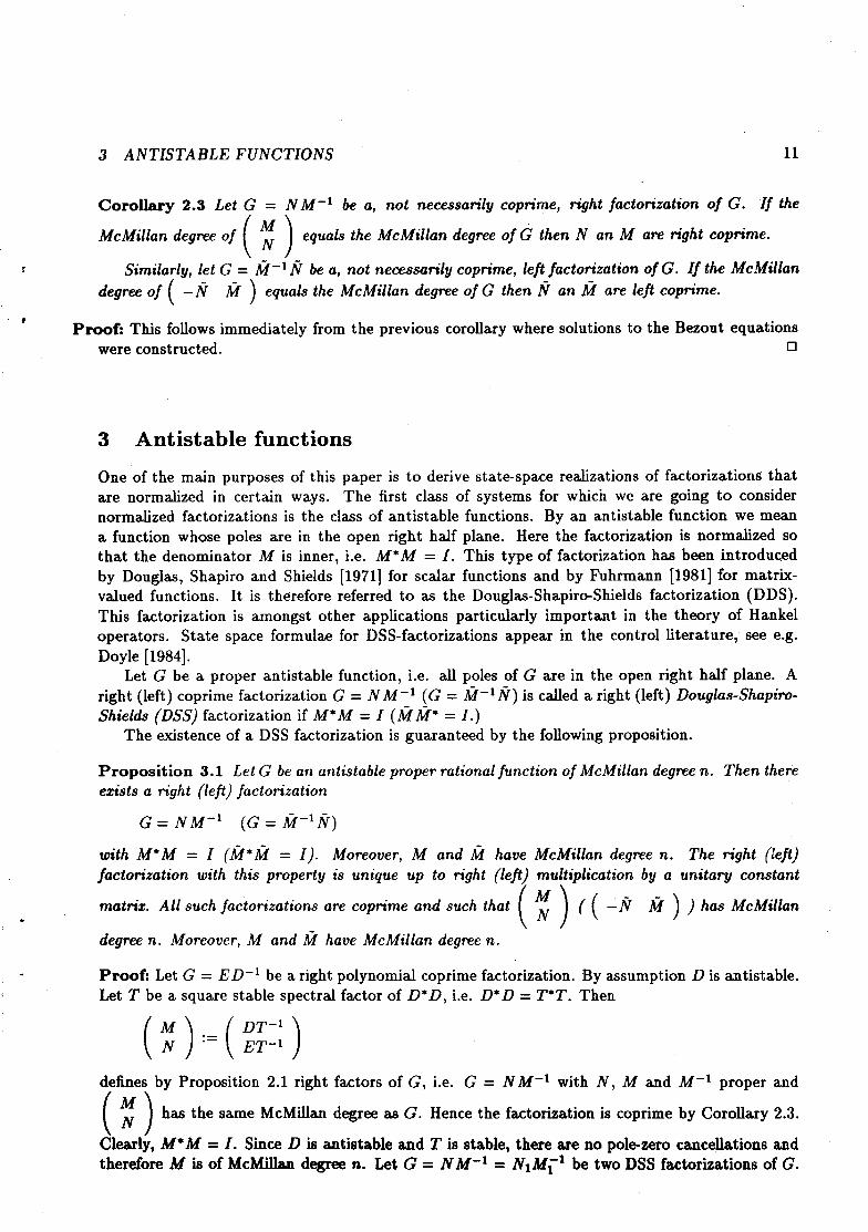
Corollary 2.3 Let G = NM-l be a, not necessarily coprime, right factorisation of G. If the
McMillan degree of M
c 1 N equals the McMillan degree of G then N an M are right coprime.
Similarly, let G = fi-lfi be a, not necessarily coprime, left factorisation of G, If the McMillan degree of ( -fi I@ ) equals the McMillan degree of G then &r an ti are left coprime.
Proofi This follows immediately from the previous corollary where solutions to the Bezout equations were constructed. cl
3 Antistable functions
One of the main purposes of this paper is to derive state-space realizations of factorizations that are normalized in certain ways. The first class of systems for which we are going to consider normalized factorizations is the class of antistable functions. By an antistable function we mean a function whose poles are in the open right half plane. Here the factorization is normalised so that the denominator M is inner, i.e. M*M = 1. This type of factorization has been introduced by Douglas, Shapiro and Shields [1971] f or scalar functions and by Fuhrmann [1981] for matrix- valued functions. It is therefore referred to as the Douglas-Shapiro-Shields factorization (DDS). This factorization is amongst other applications particularly important in the theory of Hankel operators. State space formulae for DSS-factorizations appear in the control literature, see e.g. Doyle [ 19841.
Let G be a proper antistable function, i.e. all poles of G are in the open right half plane. A right (left) coprime factorization G = NM;l (G = &f-lfi) is called a right (left) Douglas-Shapiro- Shields (DSS) factorization if M*M = I (Mi@* = I.)
The existence of a DSS factorization is guaranteed by the following proposition.
Proposition 3.1 Let G be an antistable proper rational function of McMiilan degree n. Then there exists a right (left) factorisation
G z NM--l (G z a+)
.
with M*M = I (fi*&$ = I). M oreouer, M and ti have McMillan degree n. The right (Zeft) factorisation with this property is unique up to right (left) multiplication by a unitary constant
matrix. All such factorizations are coprime and such that ((-N ti))hasMcMillan
degree n. Moreover, M and fi have McMillan degnze n.
Proof: Let G = ED-l be a right polynomial coprime factorization. By assumption D is antistable. Let T be a square stable spectral factor of D*D, i.e. D*D = T*T. Then
(;) := ($)
defines by Proposition 2.1 right factors of G, i.e. G = NM-l with N, M and Ms1 proper and M
c 1 N has the same McMillan degree as G. Hence the factorization is coprime by Corollary 2.3.
Clearly, M*M = I. Since II is antistable and T is stable, there are no pole-zero cancellations and therefore M is of McMillan degree n. Let G = NM-l = NlMi’ be two DSS factorizations of G.

3 ANTISTABLE FUNCTIONS 12
Since both are coprime factorizations, there exists a stable function Q with proper stable inverse that relates the two factorizations (see e.g. Vidyasagar [1985]). In particular, A4 = MrQ. Since 1= M*M = Q*MiMrQ = Q*Q, this shows that Q = Q-*. Since Q is stable with proper stable inverse, this implies that Q must be a constant unitary matrix.
The statement concerning left factorizations follows analogously. cl
The following Lemma wilI be important in the proofs of the main theorems of this and subse- quent sections.
Lemma 3.1 Let U(s) be a proper rationatfunction such that
U(s) = JJqs)-*J2, s c c \ o(U),
where J;, i = 1,2, are constant matrices such that Ji = J,:l = J,?, i = 1,2. Let ,?IJ E
a minimal realisation of U(s). Then,
1. D = JID-*J2.
2. U(s) has another minimal realisation of the form
-A* + C*JIDJ2B* C*JID ‘=(: :)=( DJ2B* D )’
and there exists a unique non-singular state-space transformation Y between these two real- izations such thut Y = Y *, and
YA = (-A* + C*JIDJ2B*)Y,
YB = C*JID,
C = DJ2B*Y.
Proof: Note that
and
(yJ-* x -A* + C*D-*B* C*D-*
- D-•B* D-*
and therefore
U = JIU-*J2 G -A* + C*D-*B* C”D-*J2
JID-*B*
Since U = Jl U-* Jz we clearly have that D = Jl D-* Jz. Since U E is a minimal
realization there exists a unique non-singular state-space transformation T, between this and the second realisation of U, i.e.
C = JID-*B*T,

3 ANTISTABLE FUNCTIONS 13
B = T-‘C*D-*J2,
A = T-‘(-A* + C*D-*B*)T.
Dualizing these equations, we obtain,
9 C* = T*BD-’ JI,
B* = J2D-‘CT-*,
A* = T*(-A + BD-‘C)T-*.
Solving for A, B and C we have,
C = DJ2B*T* = JID-*B*T*
B z T-•C*J1D = T-*C*D-*J2,
A = -T-•A*T* + BD-lC = -T-*AT* + T-•C*D-*J2D-‘JID-*B*T*
= T-*(-A* + C*D-*B*)T*.
But this shows that T* is also a state-space transformation between the two systems. The unique- ness of the transformation therefore implies that T* = T. The form of the realization of U given in the statement, follows immediately from the above identities. cl
.
Proposition 3.1 showed that a right (left) DSS-factorization is unique up to right multiplication
by a constant unitary matrix. The factorization is such that the McMillan degree of M
c J N
equals the McMillan degree of G. In the following theorem all doubly-coprime factorizations are
characterized which are such that M
c J N forms a DSS-factorization of G.
Theorem 3.1 Let G be an anti&able proper rational transfer function of McMillan degree n with minimal state-space realizution (A, B, C, D). Then all doubly coprime factorizations, such that G = NM-l, with MM* = I, and G = hSII? with u&f* = I, and the McMillan degrees of
( f F) and ( yN z) aren, aregivenby
. A - .ZC*C .ZC*D - B -2X*
-DiB*Y - DiDzDlC Di + DiDsDlD -DiDzDl 7 ---DID n
where DI is arbitmry such that Dl = DF*, i51 is arbitmy such that nI = nL*, Dz arbitm y, and Y and 2 are the unique positive definite solutions to the R&c& equations
AY + YA* - YBB*Y = 0,

3 ANTLSTABLE FUNCTIONS 14
A*2 + ZA - ZC*C.Z = 0.
Proof: Let G = NM-l be a DSS factorization such that A4
c J N has McMillan degree rx. This exists
by Proposition 3.1. By Theorem 2.2 any right factorization G = NM-l such has McMillan
degree n is of the form
where F is a stabilizing feedback and Dr = M(oo) is invertible. Since &i is such that M*Af = I, we have that
A4 = Iv-*.
Since M has McMillan degree n, the realization
is minimal. Lemma 3.1 now implies that there exists a unique non-singular state-space transfor- mation Y = Y* such that
PBD~ = -FEDS, . .
-F = DID;B*Y = B*Y,
%‘(A - BF) = (-A* + F*B* - F*DIDTB*)$’ = --A*p.
Using that F = - B*p we can rewrite the equation
?(A 7 BF) = -A*?
as
A*P + PA + PBB*P = 0. * Setting Y := -Y, this equation is equivalent to the more conventional equation,
A*Y + YA - YBB*Y = 0. .
Since Y is invertible, this Kccati equation is equivalent to the Lyapunov equation,
Y-‘A* + AY-’ - BB* z 0 ,
which shows that Y-l and therefore Y is positive definite. Since A* is antistable, Y-r is the unique positive definite solution of this equation. Hence Y is the unique positive definite solution to the
R,iccati equation. A state space realization of is given by

3 ANTISTABLE FUNCTIONS 15
where LIr is arbitrary such that III = LI;*.
, The expressions for the doubly coprime factors now follow from Corollary 2.2. An analogous argument or the duality consideration that G = NM-l is a right factorisation if
and only if GT = (A4T)-1N T, shows that a state space reabzation of [ -IV ti ] is given by
[ -N ii ] = A- .ZC*C ZC’D - B -ZC* Dl& -DID DI
where Z’is the unique positive solution of the Riccati equation
AZ + .ZA* - ZC*CZ = 0, ,
and Dr is arbitrary such that Dr = py*. The remaining part of the argument is analogous to tbe above derivation.
Conversely, let Y be the unique positive definite solution to the R.iccati equation
A*Y + YA - YBB*Y = 0.
Constructing the DSS factorization of G as in Proposition 3.1, proceeding as above and using the uniqueness of the solution Y, shows tbat
gives a realization of the DSS factors of G. Hence F = B*Y is a stabilizing feedback and the state-space construction gives indeed the required factorizations.
cl
The expressions for the doubly-coprime factorizations can be simplified if we are only interested in a particular factorization and not in all of them. The choice Dl = I, fl = I and Dz = 0 would lead to such a simplification.
As part of the proof of the theorem we have also shown the well-known result that a certain degenerate R,iccati equation has a stabilizing solution.
Corollary 3.1 Let (A, B, C, D) b e an antistable continuous-time minimal system. Then there exists a unique positive definite solution Y (2) of the Riccati equation
AY + YA* - YBB*Y = 0 (A*2 + ZA - ZC*CZ = 0).
This solution is such that A - BB*Y (A - ZC*C) is stable, i.e. all eigenvalues of A - BB*Y (A - ZC*C) are in the open left half plane.
Proofi This statement was proved as part of the proof of the theorem. cl

4 MINIMAL SYSTEMS 16
4 Minimal systems
Normalized coprime factorizations proved to be powerful methods in control theoretic problems, especially in the area of robust control (see e.g. Vidyasagar [1985], McFarlane and Glover [1989], Fuhrmann and Ober [1992]). For their relevance in parametrization problems, see Ober and Mc- Farlane [ 19891.
Let
A right (coprime) factorization G = NM-l of G is called a JL-RF (JL-RCF) of G if
(M* N*)(; ~)(~+w*~~+~V*IV=L
Similarly a left coprime factorization G = z-‘%r the transfer function G is called JL-LF (a JL- LCF) of G if
%W+MM*=~.
The following proposition guarantees the existence of such factorizations. The existence and uniqueness result is due to Vidyasagar (see e.g. Vidyasagar [1985]).
Proposition 4.1 Let G be a proper rational function of McMillan degree n. Then there exists a JL-right (6eft) factorisation,
G = NM-’ (G = it?+).
This factorisation is right (left) co rime and ,is unique up to right (left) multiplication by a constant p
unitary matrix. All such factorizations are such that is of McMillan degree
n.
Proofi Let G = ED-l be a right polynomial coprime factorization. Let T be a square stable spectral factor of E*E + D*D, i.e. T*T = E*E + D*D. Then
(;):=( $1:)
defines by Proposition 2.1 right factors of G, i.e. G = NM-l with N, M and M-* proper
and M
c 1 N of McMillan degree n. This also implies by Corollary 2.3 that the factorization is
coprime. Let now G = NlM;’ be another JL-right coprime factorization. Then there exists a stable Q with proper stable inverse (Vidyasagar [1985]) such that M = MlQ and N = NrQ. But I = M*M + N*N = Q*MTMlQ + Q*NiNlQ = Q*Q, w K s h* h h ows that Q = Q-*, which implies that Q is a constant matrix.
The statement concerning left factorizations follows analogously. cl
Note that for JL-factorizations G = NM-l = &-la we have that
4 MIlUMAL SYSTEMS 17
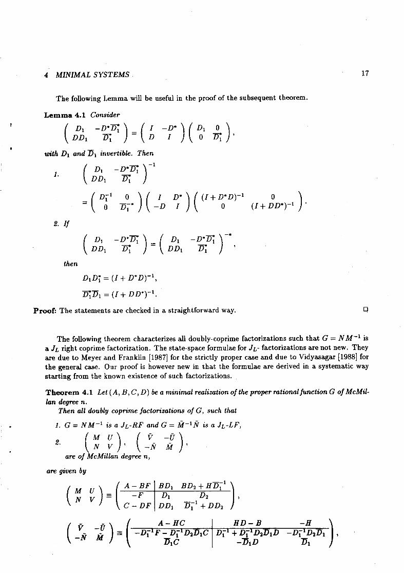
The following Lemma will be useful in the proof of the subsequent theorem.
Lemma 4.1 Consider
C ;A1 -g?)=(; -;*)( 2 g),
with Dl and nl invertible. Then
1.
then
DID; = (Z + D*D)-‘,
xi& = (Z + DD*)-‘.
Proofi The statements are checked in a straightforward way.
The following theorem characterises all doubly-coprime factorizations such that G = NM-l is a JL right coprime factorization. The state-space formulae for JL- factorizations are not new. They are due to Meyer and Franklin [1987] for the strictly proper case and due to Vidyasagar [1988] for the general case. Our proof is however new in that the formulae are derived in a systematic way starting from the known existence of such factorizations.
Theorem 4.1 Let (A, B, C, D) be a minimal realization of the proper mtional function G of McMil- lan degnze n.
Then all doubly coprime factorizations of G, such that
1. G= NM-l is a JL-RF and G = &fS1fi is a JL-LF,
2. (; ;), ( yN z),
are of h4cAfillan degree n,
are given by
(; qpJ-%y%F),

4 MIhVMA,L SYSTEMS 18
where
l III is such that DIDi = (I+ D*D)-l.
l Dl is such that flnl = (I + DD*)-‘.
a Dz is arbitrary .
l Y and .Z are solutions of the Riccati equations
0 = (A - B(I + D*D)-‘D*C)*Y + Y(A - B(I + D*D)-‘D*C)
-YB(I + D*D)-‘H*Y t C*(I t DD*)-‘C,
o = (A - B(I -+ D*D)-‘D*C)Z t Z(A - B(I t D*D)-‘D*C)*
--.X*(1 + DD*)-‘CZ •t B(I i- D*D)-‘B*,
such that A - BF and A - HC are stable, where
F = (I + D*D)-‘D*C + (It D*D)-‘B*Y,
H = BD*(I -i- DD*)-’ i- ZC*(I t DD*)-‘.
Proof: Let G have a minimal realization (A, B, C, D). Let G = NM-l be a right factorization G such that
(M* N*)JL ; =I. c )
Such a factorization exists by Proposition 4.1 and has the same McMillan degree as G. By The-
orem 2.2 any right factorization such that the McMillan degree of is the same as
where F is a stabilizing state feedback and Dl is invertible. Similarly, a left factorization G = ti-lfi such that
( -T? ti ) JL --** = I, c J
exists and is of McMillan degree n and has a state-space representation of the form
where H is a stabilizing output injection. Since is stable and of McMillan degree n and
is antistable and also of McMillan degree n, the function

4 MINIMAL SYSTEMS 19
has McMillan degree 2n. Note that since
(; -fJ-•q; --g,
we have by Lemma 3.1 that has two equivalent realisations
and
Since V = IV- l, Lemma 4.1 implies that 27 and Dl are such that
DIDi = (I + D*D)-l,
rpl = (I + DD*)-1.
We need to compute -d* + C*DB*,
-d* + C*VB*
-A*+ F*B* 0 C 0 A-HC
+ -F* (J’* - J’*D*
B-HD H )(A -;*)(: ;)(D:B* &)
-A* + F*B* 0 Z 0 A-HC
+ -F*(I + D*D) + C*D c*
B -BD* + H(I+ DD*)
Z -A* + C*DDlDiB* c*iqi&c BDl Dr B* A - BD*qD&

4 MINIMALSYSTEMS 20
Since (s) and (9) are both minimal reakations of ( f s ),
there exists a unique non-singular state-space transformation Y = , which by Lemma 3.1 ~
is such that (2: zz)= (2 2) andsuchthat
c = vt3*y,
Yd = (Ad* $ C*DB*)Y.
More explicitly, we have writing the equation Yf? = C*D componentwise,
-F* Z B-HD C*-;D*)(; -;*)(; $)
and therefore
Hence, we have that
-F*(I+D*D)+C*D = YllB,
H(I+ DD*)- BD* = YzzC*,
B=Y;B,
which shows that
F = (I+ D*D)-'D*C -(ItD*D)-'B*&, s
H = BD*(I+ DD*)-' tY&*(It DD*)-'. l
Writing Yd = (-d* t C*DB*)Y, componentwise, we have for the (1,l) entry,
YdA- BF)=(-A*tC*DDID;B*)yb +c*17;Dlcy&
and using the above identities, this gives,
O=(A*- C*DDID;B*)YlltYll(A- B[(I+D*D)-'D*C -(ItD*D)-'B*Yll])

4 MINIMAL SYSTEMS 21
Y**B(I + D*D)-*B*Y** - c*(I + my-lc.
Setting Y := -Yii we obtain the Riccati equation
0 = (A - B(1 + D*D)-‘D*C)*Y + Y(A - B(I + D*D)-‘D*C)
-YB(I + D*D)-*B*Y + c*(I + m*)-lc.
Moreover, with F = (1+ D*D)-lD*C + (1+ D*D)-lB*Y we have that A - RF is stable. Evaluating the (2,2) entry we obtain,
Yz2(-A* + C*H*) = BDlD~B*Y12 + (A - BD*DplC)Y22,
0 = (A - BD*(I + IID*)-‘C)Z + Z(A* - C*(I + DD*)-‘DB*)
--zc*(I -i- DD*)-*cz + B(1 t D*D)-lB*,
where we have set 2 := Yzz. Note that A - HC is stable with H = BD*(I i- IID*)-’ t ZC*(I t HI*)-*.
It can be verified in a straightforward but tedious way that if state space representations are -given as in the statement of the theorem that the transfer functions of these representations give doubly coprime factorizations with the required properties.
cl
In the proof of the theorem we also established the well-known result that the algebraic Riccati equation has a stabilizing solution.
Corollary 4.1 Let (A, B, C, II) be a minimal continuous-time system. Then there exist hermitian solutions Y and 2 of the Riccxti equations
0 = (A - B(I+ D*D)-‘D*)*Y t Y(A - B(1 t D*D)-‘D*C)
-YB(I t D*D)-*B*Y + c*(I -I- m*)-*c,
respectively,
0 = (A - B(I+ D*D)-lD*C)Z t Z(A - B(1 t DV)-‘D*C)*
-zc*(I i- m*)-*cz -t B(1 j- D*D)-*B*,
such that A - BF and A - HC are stable, where
F = (I+ D*D)-‘D*C -t (I •t- D*D)-‘B*Y
H = BD*(I t DD*)-’ t X*(1 t DD*)-‘.
Proofi This statement was prcved as part of the proof of the theorem.
5 BOUNDED-REAL FUNCTIONS 22
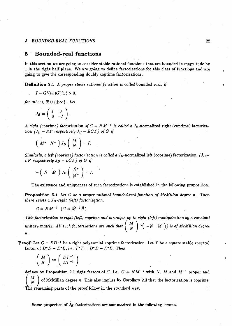
5 Bounded-real functions
In this section we are going to consider stable rational functions that are bounded in magnitude by 1 in the right half plane. We are going to define factorizations for this class of functions and are going to give the corresponding doubly coprime factorizations.
Definition 5.1 A proper sta6le rational function is called bounded real, if
I - G*(iw)G(iw) > 0,
for idi w E 8? U {ho}. Let
A right (coprime) factorisation of G = NA4-r is called a JB-normabzed right (coprime) factoriza- tion (JB - RF respectively JB - RCF) of G if
(M* N* ) JB r = I. c )
Similarly, a Zeft (coprime) factorisation is called a ..JB-norm&zed left (coprime) factorization (JB - LF respectively JB - LCF) of G if
The existence and uniqueness of such factorizations is established in the following proposition.
Proposition 5.1 Let G be a proper rational bounded-ma1 function of McMiUan degree n. Then there exists a JB-right (left) factorisation,
G = NM-’ (G = A?-‘@.
This factorisation is right (left) co p rime and is unique up to right (left) mu&p&cation by a constant
unitary matrix. AH such factorizations are such that is of McMillan degree
n.
Proofi Let G = ED-l be a right polynomial coprime factorization. Let T be a square stable spectral factor of D*D - E*E, i.e. T*T = D*D - E*E. Then
defines by Proposition 2.1 right factors of G, i.e. G = NiU-l with N, h4 and iki-1 proper and M
c ) N of McMillan degree n. This also implies by Corollary 2.3 that the factorization is coprime.
The remaining parts of the proof follow in the standard way. cl
Some properties of JB-factorizations are summxti in the following lemma.

5 BOUNDED-REAL FUIVCTIONS 23
Lemma 5.1 Let G = Nh4-1 6e a JB-RF and G = fimlN a JB-LF of the stable bounded-real function G. Then
1.
2. (F ;~)=JB( z iI)-*JB.
Proofi The statements are easily verified. cl
The following Lemma will be useful in the proof the subsequent theorem.
Lemma 5.2 Consider
C ;il L$y)=(; ?)(;I &),
with D1 and n1 inuertible and D such that I - DD* > 0. Then
-1
1. D1 D*fl
DD1 q
2. If
D1 D*??; D1 D*q -*
DD1 F DD1 q JB,
then
DID; = (I- D*D)-‘,
qDl = (I - DD*)-‘.
Proof: The statements are checked in a straightforward way. cl
We are now in a position to characterise all doubly coprime factorizations so that G = N M-‘( = %$-la) is a JB-RF (JB-LF).
Theorem 5.1 Let (A, B, C, D) be a minimal realisation of the proper bounded-real mtional function G of iUch4illan degree n.
Then all doubly coprime factorizations of G, such that
1. G = NM-’ is a JB-RF and G = tiWIH is a JB-LF,
2% (; ;), (TN z),
am of iUcMllan d&fee n,
5 BOUNDED-REAL FUNCTIONS 24
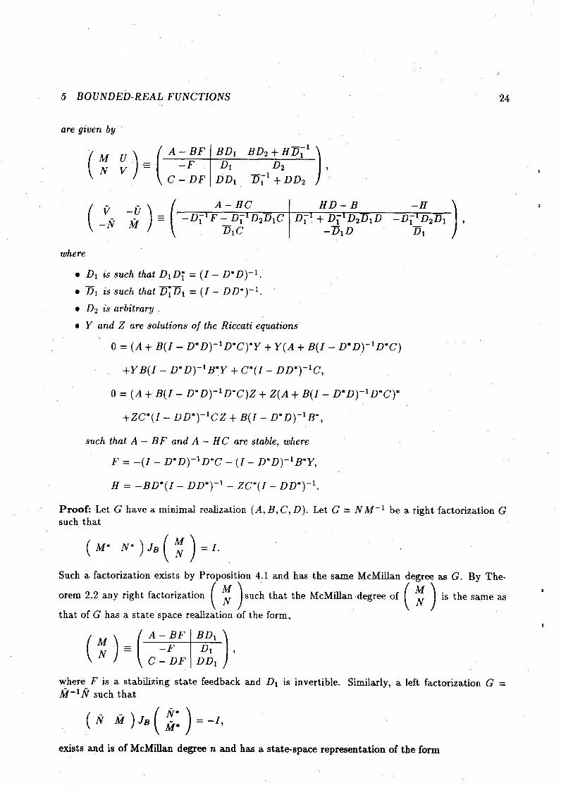
are given by
(; ;)+fJjyYF)7 &
’
where
l Dl is such that DIDi = (I - D*D)-‘.
l Dl is such that ~DI = (I - DD*)-I.
l D2 is arbitrary .
l Y and 2 are so&ions of the Riccati equations
0 = (A + B(I- D*D)-‘D*C)*Y + Y(A + B(I- D*D)-‘D*C)
+YB(I - D*D)-‘B*Y + C*(I - DD*)-‘C,
0 = (A + B(I- D*D)-‘D*C)Z + .Z(A + B(I- D*D)-‘D*C)*
i-ZC*(I - DD*)-‘CZ t B(I- D*D)-‘B*,
such that A - BF and A - HC are stable, where
F = -(I - D*D)-‘D*C - (I - D*D)-‘B*Y,
H = -BD*(I - DD*)-’ - ,X*(1 - DD*)-I.
Proof: Let G have a minimal realization (A, B,C, D). Let G = NM-’ be a right factorization G such that
( M* N* ) JB
Such a factorization exists by Proposition 4.1 and has the same McMillan degree as G. By The-
orem 2.2 any right factorization M
c 1 N such that the McMillan ‘degree of is the same as
that of G has a state space realization of the form,
where F is a stab&zing state feedback and Dl is invertible. Similarly, a left factorization G = &f-lfi such that
exists and is of McMillan degree n and has a state-space representation of the form

5 BOUNDED-REAL FUNCTIONS 25
.
where H is a stabilizing output injection. Since M c ,J N is stable and of McMillan degree n and
is antistable and also of McMillan degree n, the function
A-BF 0 0 -A* + C*H*
-F D*H*wB* C-DF H*
has McMillan degree 2~. Note that since
(; ;:) =JB(; ;:)-*J*,
we have by Lemma 3.1 that has the two equivalent realizations
and
-A* + C*JB’DJBB* C*JBV ‘DJBB*
Since D = J~i9-l JB, Lemma 4.1 implies that D and DI are such that
DID; = (I - D*D)-‘,
qzl = (I - DD*)-‘. *
We need to compute -A* + C*JBV JBB*,
. -A* + C*JBVJBB*
-A*+ F*B* 0 Z 0 .A-HC
+ -F* HD-B
-A*+ F*B* 0 Z 0 A-HC
LJnlv.-abi. wm3iautfJra

5 BOUNDED-REAL FUNCTIONS 26
t -F*(I - D*D) - C*D c* -B BD* t H(I- DD*)
-A* - C*DDlDiB* c*Dp1 c t Z
-BDlDiB* A j- BD*qn& ’
-A* +- C*JBVJBB* C*JBV si~ce (s) and ( vJ~t?* V )
arebothminirnalreakationsof ( t i: ), ’
there exists a unique non-singular state-space transformation Y =
is such that (‘2: zi)= (2 2 ),andsuchthat
which by Lemma 3.1
C = VJBB*Y,
YB = C*JBV,
YA = (-A* t C*JBVJBB*)Y.
More explicitly, we have writing the equation YB = C*JB’D componentwise,
C -F* Z HD-B c*-;*D*) (-; :;) (; ;;)
and therefore
Hence, we have that
-F*(I - D*D) - C*D = YllB,
-c* = Y&*,
-H(I - DD*) - BD* = Y&‘*, c
-B = Y;B, a
which shows that
F = -(I - D*D)-‘D*C - (I - D*D)-‘B*Yll,
H = -BD*(I - DD*)-’ - Y&*(1 - DD*)-‘.
Writing YA = (-A* + C*JBVJBB*)Y, componentwise, we have for the (1,l) entry,
Yll(A - BF) = (-A* - C*DDID;B*)Yll + C*D;n&Y&,
and using the above identities, this gives,
5 BOUNDED-REAL FUNCTIONS 27
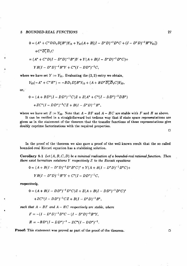
0 = (A* + C*DDlDiB*)Yll + Yll(A + B[(I - D*D)-‘WC + (I - D*D)-‘B*Yll])
+C*FD1C
s = (A* t C*D(I - D*D)-‘B*)Y -+ Y(A +- B(I - D*D)-lD*C)+
. YB(I- D*DyB*Y -+ c*(I - myc,
where we have set Y := Yrt. Evaluating the (2,2) entry we obtain,
Yzz(-A* + C*H*) = -BDlDiB*Ylz + (A + BD*~~~C)Y&,
0 = (A t BD*(I - DD*)-‘C)Z t Z(A* t C*(I - DD*)-‘DB*)
+X*(1 - DD*)-Yz + B(I - ml)-98,
where we have set 2 := Yzz. Note that A - BF and A - HC are stable with F and H as above. It can be verified in a straightforward but tedious way that if state space representations are
given as in the statement of the theorem that the transfer functions of these representations give doubly coprime factorizations with the required properties.
Cl
In the proof of the theorem we also gave a proof of the well-known result that the so called bounded-real R,iccati equation has a stabilizing solution.
Corollary 5.1 Let (A, B, C, D) 6 e a minimal realizution of a bounded-ma1 rational function. Then there e&t hermitian solutions Y respectively 2 to the Riccati equations
0 = (A + B(I- D*D)-lD*B*C)* t Y(A t B(I - D*D)-‘D*C)+
YB(I- D*lyB*Y + c*(I - m*)-w,
respectively,
0 = (A t I?(1 - DD*)-‘D*C)Z + .Z(A t B(I - DD*)-‘D*C)*
+ZC*(I - DD*)-*cz -j- B(I - ll*q-II?*,
such that A - BF and A - HC respectively are stable, where
F = -(I - D*D)-‘D*C - (I - D*D)-lB*Y,
H= -BLqI - IID*)- - 2x*(1 - DD*)-1.
Proof: This statement was proved as part of the proof of the theorem. cl
6 POSITIVE-REAL FUNCTIONS 28
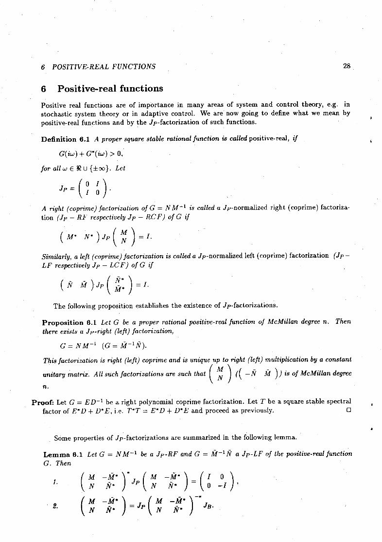
6 Positive-real fund ions
Positive real functions are of importance in many areas of system and control theory, e.g. in stochastic system theory or in adaptive control. We are now going to define what we mean by positive-real functions and by the Jp-factorization of such functions.
Definition 6.1 A proper square stable rational function is called positive-real, if
G(iw) + G*(iw) > 0,’
for all w E $2 U {km}. Let
A right (coprime) factorisation of G = NA4-1 is called a Jp-normahzed right (coprime) factoriza- tion (JP - RF respectively Jp - RCF) of G if
(M* N*)Jp ; =I. c )
Similarly, a lefi ( co rime) factorisation is called a Jp-normalized left (coprime) factorization (JP - p LF respectively Jp - LCF) of G if
The following proposition establishes the existence of Jp-factorizations.
Proposition 6.1 Let G be a proper rational positive-real function of McMillan degree n. Then there exists a JP-right (left) factorisation,
G = NM-’ (G = ti-‘fi).
This factorisation is right (left) co rime and is unique up to right (left) multiplication by a constant p
unitary matrix. All such factorizations are such that is of McMillan degree
n.
Proof: Let G = ED-l be a right polynomial coprime factorization. Let T be a square stable spectral factor of E*D + D*E, i.e. T*T = E*D + D*E and proceed as previously. cl
Some properties of Jp-factorizations are summarized in the following lemma.
Lemma 6.1 Let G = NM-l be a JP-RF and G = fi-lfl a Jp-LF of the positive-real function G. Then
I. (; -;*)*JP(: -$*)=(; !*),
2. (; -f*)=Jp(; -$*)-*JB.

6 POSITIVE-REAL FUNCTIONS
Proofz The statements are easily verified.
29
cl
.
A fey useful identities are given in the following Lemma.
Lemma 6.2 Consider
C ;A1 ;*s)=(; ;!)(; ;J
with Dl and Dl invertible and D is square such that D + D* > 0. Then -1
1. D1 -D;
DD1 D*r
2. If
JB,
then
DID; = (D + D*)-‘,
qDl = (D + D*)-‘.
Proof: The statements are checked in a straightforward way. cl
We can now characterise doubly coprime factorizations for positive-real functions.
Theorem 6.1 Let (A, B, C, D) b e a minimal realisation of the proper positive-real rational function G of h4cMiiian degree n.
Then ail doubly coprime factorizations of G, such that
1. G = NM-l is a JP-RF and G = timlfi is a JB-LF,
2. (: ;), (TN ;),
are of McA4illan degree n.
are given by

6 POSITIVE-REAL FUNCTIONS 30
where
l Dl is such thut DID; = (D + D*)-I. l i?l is such that ~DI = (D + D*)-l. l Dz is arbitrary . l Y and .Z are solutions of the Riccati equations
0 = (A - B(D + D*)-‘C)*Y t Y(A - B(D + D*)-‘C)
tYB(D t D*)-‘B*Y + C*(D t D*)-‘C,
0 = (A - B(D t D*)-‘C)Z t Z(A - B(D t D*)-IC)
tzC*(D + D*)-%‘.Z i- B(D -+ D*)-lB*,
such that A - BF and A - HC are stable, with
F = (D t D*)-‘C - (D + D*)-‘B*Y,
H = B(D t D*)-’ - ZC*(D + D*)-‘.
Proof: Let G have a minimal realization (A, B, C, D). Let G = NA4-* be a right factorization G such that
(M* N* ) Jp ; = I. c )
Such a factorization exists by Proposition 4.1 and has the same McMillan degree as G. By ‘Pheo-
rem 2.2 any right factorization such that the McMillan degree of is the same as
that of G has a state space realization of the form,
where F is a stabilizing state feedback and Dl is invertible. Similarly, a left factorization G = &#-lfi such that
exists and is of McMillan degree n and has a state-space representation of the form
where H is a stabilizing output injection. Since is stable and of McMillan degree n and
is antistable and also of McMillan degree n, the function

6 POSITWE-REAL FUNCTIONS 31
.
-. -.
has McMillan degree 2n. Note that since
we have by Lemma 3.1 that A4 N
-&f* -* N
has the two equivalent retizations
and
-d* + C*J~VJBB* C* JpV VJBB* J v -
Since V = JpVe* JB, Lemma 4.1 implies that V and Dl are such that
DID; = (D t D*)-l,
Dpl = (D t D*)-l.
We need to compute -d* + C*J~VJBB*,
-d* + C*J~VJBB*
-A* + F*B* 0 Z 0 A-HC
+ -F* C* - J'*D* -H HD-B )Jp(; ;f)( 2 ;;)JB(Dr* &)
C
-A* i- F*B- 0 Z 0 A-HC 1
t C
-J’* C* - J’*D* -H HD-B )(: -:*)(DiDi $j&)(: :)
-A* + F*B* 0 Z 0 A-HC
+ -F*(D + D*) + C’* C’ -B H(D+D*)-B

6 POSITIVE-REAL FUNCTIONS 32
E -A* + C*DID;B= C*iJp& -BDl D;B* A-BD;D&
-A* +C*J~‘DJBU* C*JpD sin” (s) and ( DJB~~* ‘D )
arebothminimalrealizationsof ( T -K* ), ’
there exists a unique non-singular state-space transformation Y = which by Lemma 3.1 ,
is such that (2: zz)= ($ E),andsuchthat
C = VJB~?*Y,
YB = C*JpV,
YA = (-A* + C8Jp’DJ~f3*)Y.
More explicitly, we have writing the equation Yf3 = C*JpIV componentwise,
-F* C* - F*D* HD-B )(; ;)(h ;!)(? i;)’
and therefore
;;) ( f &) = ( -F*‘D;;*“+c* -Y&&+B)’
Hence, we have that
-F*(D + D*) + C* = YllB,
-H(D + D*) + B = YnC*,
-B = Y;B,
which shows that
F = (D + D*)-‘C - (D + D*)-’ B*Yll,
H = B(D + D*)-’ - Y&*(D + D*)-‘.
Writing YA = (-A* + C*J~~VJBB*)Y, componentwise, we have for the (1,l) entry,
YII(A - BF) = (-A* + C*DID;B*)Yll + C*c?%CY;z,
and using the above identities, this gives,
0 = (A* - C*DID;B*)Yll + Yll(A - B[(D + D*)-'C + (D + D*)-'B*Yh])

7 REFERENCES 33
= (A* - C*(D + D*)-‘B*)Y + Y(A -- B(D + D*)-lC)-+
YB(D •t II*)-*B*Y -t c*p -I- rye, ’ !
where we have set Y := Yii. Evaluating the (2,2) entry we obtain,
. Y&-A* t C*H*) = -BDID;B*Y12 i- (A - BD;DIC)Yz2,
or,\
0 = (A - B(D + II*)-‘C)Z + Z(A* - C*(L) -I- D*)-lB*)
tZC*(D + D*)-lcz -I- B(D -I- D*)-*B*.
The remaining part of the proof is anaIogous to the equivalent steps in the previous theorems. 0
In the proof of the theorem we also estabiished the weiI-known result that positive-reaI Riccati equations have a stabihzing solution.
Corollary 6.1 Let (A, B, C, II) be a minimal realisation of a positive-real rational function. Then there exist hermitian solutions Y respectively .Z to the Ricati equations
0 = (A* - C*(D -t D*)-‘B*)Y + Y(A - B(D t D*)-‘C)t
YB(D i- D*)-*B*Y + c*p i- II*)-*c.
respectively,
0 = (A - B(D -t D*)-‘C)Z i- Z(A* - C*(D +- II*)-‘B*)
-i-zc*(D •t D*)-*.z -I- B(D + II*)-*B*.
such that A - BF and A - HC are stable, where
F = (D t D*)-‘C - (D t D*)-‘,
H = B(D t II*)-’ - .W*(D t II*)-‘.
Proof: This statement was proved as part of the proof of the theorem.
7 REFERENCES
[1949] A. Beurling. “On two problems concerning Iinear transformations in HiIbert Space”. Acta Math., 81,239-255.
[1980] Demer, C.A., R.W. Liu, J. Murray and R. Sacks. “Feedback system design: the fractional representation approach”, IEEE TAC, 25,399-412.

7 REFERENCES 34
[1971] R.G. D ou gl as, H.S. Shapiro and A.L Shields. “CycIic vectors and invariant subspaces for the backward shift.” Ann. Inst. Fourier, Grenoble, 20,1, 37-76.
[1984] J.C. Doyle, ” Lecture Notes in Advances in Multivariable Control”, ONR/HoneyweII Workshop, MinneapoIis, MN.
a
[1975] P. A. Fuhrmann, “On Hankel operator ranges, meromorphic pseudo-continuation and factorization of operator vahred analytic functions”, J. Lond. M&h. Sot., (2) 13, 323-327.
[1976] P. A. Fuhrmann, “Algebraic system theory: An analyst’s point of view”, J. Fmnklin Inst., 301, 521-540.
[1979] P. A. Fuhrmann, “Linear feedback via polynomial models”, 1&. J. Contr. 30, 363-377.
[1981] P. A. F h u rmann, Linear Systems and @er&ors in Hr%ert Space, McGraw-HiII, New York.
[1985] P. A. Fuhrmann, “The algebraic Riccati equation - a polynomiai approach”, S’yst. und Contr. Lett., 369-376.
[1991] P. A. Fuhrmann, “ A polynomial approach to Hankel norm and balanced approximation”, Lin. Alg. Appl., 146, 133-220.
[1992] P. A. F u h rmann and R. J. Ober, “A functional approach to LQG baIancing”, to appear in International Journal of Control.
[1985] J. Hammer, “No&near systems, stabiiization, and coprimeness”, Internationaf JournaZ of Control, Vol. 42, pp. 1 - 20.
[1978] M. L. J. Hautus and M. Heymann, “Linear feedback-an aigebraic approach”, SIAM J. Control 16, 83-105.
[1980] T. Kailath, Linear systems, Prentice Ha& Englewood CIiffs, N.J.
[1982] P. Khargonekar and E. Sontag. “On the relation between stable matrix factorizations and regulable reahzations of Iinear systems over rings”, IEEE TAC, 27, 627-638.
[1989] D. M F 1 c ar ane and K. Glover, “Robust controher design using normahzed coprime factor plant descriptions”, Lecture Notes in Control and Information Sciences, vol. 10, Springer Verlag.
[1987] D. M e y er and G. Frankhn, “A connection between normahzed coprime factorizations and Iinear quadratic regulator theory”, IEEE Tmns. on Auto. Contr. 32, 227-228.
[1975] A. S. Morse, “System invariants under feedback and cascade control”, Lecture Notes in Economics and Muthematicaf Systems, vol. 131 (Proc. Symp. Udine), Springer Verlag.
[1984] C.N. Nett, C.A. Jacobson and M.J. B&s. ” A connection between state-space and doubly coprime fractionai representations”. IEEE TAC, 29, 831-832.
[1989] R.J. Ober, D-C. .McFarlane. “Balanced canonical forms: a normalised coprime factor approah.” Linear Algebra and its Applications, 122-124: 23-640.

7 REFERENCES 35
[1970] H. H. R osenbrock, State Space and Multiuariable Theory, J.Wiley, New York.
[1988] M.S. Verma, “Coprime Fractional Representations and Stability of Nonlinear Feedback Systems”, International Journal of Control, 48, 897-918.
[1985] M. Vidyasagar, Control System Synthesis: A Coprime Factorisation Approach, M.I.T. Press, Cambridge MA.
[1988] M. Vidyasagar. “Normalized coprime factorizations for non strictly proper systems”. Automatica, 85-94. p/J 2 VI+
[1976] D. C. Youla, J. J. Bongiorno and H. A. Jabr, “Modern Wiener-Hopf design of optimal controllers, Pt. 2 The multivariable case”, IEEE Transactions on Automatic Control, 21, 319338.