fortran codes for estimating the one-norm of a real or ...higham/narep/narep135.pdf · where the...

FORTRAN Codes for Estimating the One-Norm of a Real or Complex Matrix, with Applications to Condition Estimation

NICHOLAS J. HIGHAM University of Manchester

FORTRAN 77 codes SONEST and CONEST are presented for estimating the l-norm (or the m- norm) of a real or complex matrix, respectively. The codes are of wide applicability in condition estimation since explicit access to the matrix, A, is not required; instead, matrix-vector products Ax and A “‘n are computed by the calling program via a reverse communication interface. The algorithms are based on a convex optimization method for estimating the l-norm of a real matrix devised by Hager [Condition estimates. SIAM J. Sci. Stat. Comput. 5 (1984), 311-3161. We derive new results concerning the behavior of Hager’s method, extend it to complex matrices, and make several algorithmic modifications in order to improve the reliability and efficiency.

Categories and Subject Descriptors: G.1.3 [Numerical Analysis]: Numerical Linear Algebra

General Terms: Algorithms

Additional Key Words and Phrases: Condition estimation, condition number, convex optimization, FORTRAN, infinity-norm, LINPACK, one-norm, reverse communication

1. INTRODUCTION

Hager [ll] presents a method for estimating the l-norm of a real matrix B, with particular reference to estimating (1 A-’ 11 , and, hence, the matrix condition number ~~ (A) = I] A 1) 1 I] A-’ ]I 1. Th e method has the very useful property that its dependence on B can be isolated in references to a “black box,” whose defining property is that given an input vector x it returns either Bx or B TV. This property implies that a single “universal” code can be written that is applicable to any matrix, whether it is given explicitly or implicitly; to apply the code to a particular matrix, one simply provides a means to evaluate the required matrix-vector products. Hence, in the context of condition estimation, one code can serve as a condition estimator for all possible factorization routines and linear equation solvers. This contrasts with the LINPACK condition estimation algorithm, which makes direct access to elements in a factorization of the matrix and thus requires specific code to be written for each particular factorization routine.

Author’s address: Department of Mathematics, University of Manchester, Manchester, Ml3 9PL, England. Permission to copy without fee all or part of this material is granted provided that the copies are not made or distributed for direct commercial advantage, the ACM copyright notice and the title of the publication and its date appear, and notice is given that copying is by permission of the Association for Computing Machinery. To copy otherwise, or to republish, requires a fee and/or specific permission. 0 1988 ACM 0098-3500/88/1200-0381$01.50

ACM Transactions on Mathematical Software, Vol. 14, No. 4, December 1986, Pages 381-396.

382 l Nicholas J. Higham

This very attractive feature of Hager’s method, which is not explicitly noted in [ll], motivated the present work in which we develop FORTRAN codes based on Hager’s method. The codes will be of particular interest in contexts where the LINPACK condition estimation algorithm is not available-either because it is not applicable or because the algorithm has not yet been implemented. An example of the former case is the problem of estimating the norm of a matrix- matrix product without forming the product: for example, ABC, or A-‘B (where a factorization of A is available). Three applications in which the LINPACK algorithm has in some cases not been implemented are as follows:

(1) sparse matrix packages (though see [2], [6], [lo], and [22]); (2) program libraries specially written for solving linear equations on a high-

performance computer [5, 151; and (3) software for solving Sylvester equations AX + Xl3 = C, where A is m x m

and B is n X n: These linear equations may be expressed in the form Px = c, where the Kronecker sum P = I,@ A + BT @ I,,,. As shown in [9] and [13], an estimate of a norm of P-l is useful for assessing the accuracy of a computed solution. Hager’s method is appropriate for estimating ]I P-l 11 1 since the matrix-vector products P-lx and PeTx are the solutions to further Sylvester equations, which can be computed using whatever method is used to solve the original Sylvester equation (be it a direct matrix factorization method [9, 131 or an iterative method [ 161). We mention that LINPACK style condition estimators for use with Schur methods for solving Sylvester and generalized Sylvester equations have recently been developed by Byers [l] and by Kdgstrijm and Westin 1171.

In both (1) and (2), having a single condition estimation routine that is called by all the factorization routines yields obvious economy of space and implementation effort. Furthermore, the nature of our codes is such that they require little or no tailoring for special storage schemes or computer architectures.

We mention that FORTRAN codes implementing the original version of Hager’s method [II] are available in NAPACK; this package is documented in [ 123, and individual routines can be obtained from NETLIB [4]. NAPACK contains a general-purpose matrix l-norm estimation routine NORM& as well as several condition estimation routines geared to particular matrix types, such as general real, banded, symmetric, and tridiagonal.

This paper is organized as follows: In Section 2 we describe Hager’s method and derive new results concerning its behavior. In particular, we present several “counterexamples” on which the method performs badly.

In Section 3 we describe extensive numerical experiments with the method that give insight into its behavior in practice. Based on this experience, we suggest in Section 4 several algorithmic refinements, which help to improve the reliability and efficiency. These combine to yield Algorithm 4.1, which forms our practical algorithm for l-norm estimation of real matrices.

In Section 5 we extend Hager’s method to complex matrices. Section 6 contains details of the FORTRAN codes and some test results. Finally, in Section 7 we discuss the computational cost and reliability of the codes. ACM Transactions on Mathematical Software, Vol. 14, No. 4, December 1988.

FORTRAN Codes for Condition Estimation 383

Recall that the l-norm of A E R”“” is given by

where I] x ]I 1 = Cj ] xj ] , and that the same expressions hold when R is replaced by C. Since the m-norm of A E R”“” or C”“” satisfies 11 A 11 m = 11 A ’ 11 1, it follows that the algorithms and codes given here can be used to estimate the m-norm by applying them to the transposed matrix.

We note that, although we consider only square matrices here, it is sometimes desirable to estimate the l-norm of a rectangular matrix. One approach is to work with the square matrix obtained by padding the rectangular matrix with zeros.

In our presentation we will variously consider the problem to be that of estimating I] B ]I 1, or I( A-l I] ,-the former notion is the more general, whereas the latter reflects the problem of most practical interest.

2. HAGER’S ALGORITHM

For B E REX”, I] B 1) 1 is the global maximum of the convex function

0) = II Bx II I over the convex set

This suggests using an optimization approach to estimate I] B ]I 1 : Iteratively move from one point in S to another where F is greater, testing for optimality at each stage. Hager [ll] derives such an algorithm by exploiting properties of F and S as follows: At points x E S where Bx has no zero components, F is differentiable and, in fact, locally linear; so, for y E S with )I y - x I( sufficiently small,

F(Y) = F(x) + VFblT(y - xl, (2.1)

where VF is the gradient vector of F. If I] VF(x) I) m I VF(X)~X, then, since ] VF(X)~Y ] I 1) VF(x) ]I m I] y ]I 1 5 I] VF(x) I] m, it follows from (2.1) that x is a local maximum of F over S.

If (BX)i = 0 for some i, then F is not differentiable at x. However, the convexity of F and S ensures that vectors g exist such that

F(Y) 2 F(x) + gT(y - x) for all y E S. (2.2)

Vectors g satisfying (2.2) are called s&gradients of F (see, e.g., [B, p. 1791). Inequality (2.2) suggests the strategy of choosing a subgradient g and moving

from x to a point y* E S that maximizes g T( y - x). Since ] g Ty ) 5 I( g (1 m and since F(y) = F(-y), it follows that we can take y* = e; , where ] gj ] = I] g ]I m and ej is the vector with 1 in the jth position and zeros everywhere else. If ]I g ]I m > gTx, then F(y*) > F(x) is assured. Note that by convexity theory, or simply from (l.l), the global maximum of F is attained at one of the vertices cj .

ACM Transactions on Mathematical Software, Vol. 14, No. 4, December 1988.


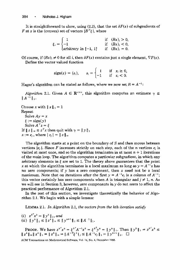
It is straightforward to show, using (2.2), that the set dF(x) of subgradients of F at x is the (convex) set of vectors (Brt }, where

[; =

i

-: if (BX)i > 0, if (BX)i < 0,

arbitrary in [-1, l] if (Bx)i = 0.

Of course, if (Bx)~ # 0 for all i, then dF(x) contains just a single element, VF(x). Define the vector valued function

sign(x) = (si), 1 1 si =

if Xi Z 0, -1 if Xi < 0.

Hager’s algorithm can be stated as follows, where we now set B = A-l:

Algorithm 2.1. Given A E R""", this algorithm computes an estimate y 5 II A -’ II I.

Choose x with 11 x 11 1 = 1 Repeat

Solve Ay = x 4 := sign(y) Solve A TV = E

If 11 z 11 m 5 zTx then quit with y = II y II 1 x:=ej,where lzjl = 11~11,

The algorithm starts at a point on the boundary of S and then moves between vertices {ej ). Since F increases strictly on each step, each of the n vertices ej is visited at most once, and so the algorithm terminates in at most n + 1 iterations of the main loop. The algorithm computes a particular subgradient, in which any arbitrary elements in 5 are set to 1. The theory above guarantees that the point x: at which the algorithm terminates is a local maximum as long as y = A-‘z has no zero components; if y has a zero component, then x need not be a local maximum. Note that on iterations after the first y = A-‘ej is a column of A-‘; this vector certainly has zero components when A is triangular and j # 1, n. As we will see in Section 3, however, zero components in y do not seem to affect the practical performance of Algorithm 2.1.

In the rest of this section, we investigate theoretically the behavior of Algo- rithm 2.1. We begin with a simple lemma:

LEMMA 2.1. In Algorithm 2.1, the vectors from the kth iteration satisfy

(i) zhTx” = 11 yk II I, and (ii) II yk II 1 5 II zk II- 5 II yk+’ II I 5 II A-l III.

PROOF. We have zkTxk = tkTA-‘xk = tkTyk = 11 yk 11 1. Then 11 yk 11 1 = zkT3tk 5 II.z~I~~~~x~II~= II~~llm= IA-T[kjj~ IIA-‘ejII1= IIyktlII1. 0 ACM Transactions on Mathematical Software, Vol. 14, No. 4, December 1988.

FORTRAN Codes for Condition Estimation l 385

The lemma reveals the interesting property that on every iteration the w-norm of the subgradient z is an estimate of ]] A-’ ]] 1 that is at least as good as F(x) = ]] y (] 1. However, on the last iteration the two estimates are the same, since the convergence test may be expressed as “if I] z ]I m = ]I y I] 1.” Thus, there is no advantage to be gained from using the estimates I( z ]I m (unlike for the LINPACK estimator where additional estimates of a similar kind prove to be useful [20]).

The lemma admits a heuristic interpretation of Algorithm 2.1. On stages after the first y is a column of A-‘, the kth, say, and [ is the sign pattern of this column. The element zi is the inner product of this sign pattern with the ith column of A-‘. If there is equality in I( y (] 1 = ] zk ] I (I z ]I .,,, then it is reasonable to assume that the kth column has the largest l-norm and to terminate the algorithm; otherwise, thejth column, where ] sj ] = ]I z ]I .,,, has a larger norm than the kth and is a likely candidate for being the column with the largest norm, so this column should be computed next.

A natural choice of starting vector, in the absence of any special knowledge about A, is n-‘e, where e = (1, 1, . . . , 1)r. This vector is equivalent to any other of the form n-ld, di = +l, in the following sense: If the algorithm is applied to A with starting vector n-‘e, it produces the same estimate, after the same number of iterations, as if it is applied to DAD with starting vector n-ld, where D = diag(di). We will assume the starting vector is n-‘e in the rest of this section.

An interesting special case for Algorithm 2.1 is when A-l 10, as, for example, when A is an M-matrix. It is easy to see that on the first iteration (] z (I m = IA-‘II,, and so by Lemma 2.1 the algorithm terminates after at most two iterations with an exact estimate. Note that if a second iteration is used then 4 = e, as on the first iteration, and so Algorithm 2.1 solves the system ATz = e twice. We return to this point in Section 4.

Now we examine some “counterexamples’‘-matrices where Algorithm 2.1 performs badly; these expand on the single counterexample given in [14]. Con- sider first the Pei matrices [21]

A = crl+ eeT, a 2_ 0. (2.3)

Using

A-’ = a-‘I - 1 eeT, II A-’ II 1 =

Ly + 2(n - 1)

a(a + n) cY(a+n) ’

we find that, in the first stage of Algorithm 2.1, y = A-‘(n-‘e) = n-‘(a + n)-‘e, and thus, 4 = e and z = A-‘e = (cy + n)-‘e. Hence, the algorithm terminates on the first stage at a local maximum. The estimate is y = I] y ]I 1 = (a + n)-‘, and the underestimation ratio is

CY ff + 2(n - 1)

-+O as (Y + 0 and/or n + w.

Thus, for the Pei matrices the local maximum computed by Algorithm 2.1 can be an arbitrarily poor approximation to the global maximum.

ACM Transactions on Mathematical Software, Vol. 14, No. 4, Dwember 1988.

386 - Nicholas J. Higham

Our next example is the bidiagonal matrix B,:

(1 1 -1 1 . . . (-1y+l

1 1 -1 .

1 1

B, = 1 ** , B,l = 1 ** .

* (2.4) *.

*. 1 -1

\ 1 1,

On the first iteration, y = n-l (1, 0, 1, 0, . . . )T if n is odd; else, y = n-l (0, 1, 0, 1 . . )r. Thus, [ = e and z = BiTe = (1, 0, 1, 0, . . . )? The convergence condition ii not satisfied. If we take the smallest j such that ] zj ] = I( z ]I m, then x = el for the second iteration, giving y = el, and [ and z as on the first iteration. The algorithm now has converged, and it returns y = I] y ]I 1 = 1, so that

we have a poor estimate unless n is small. Note that the final y has zero elements; it is easily confirmed that the stopping vertex x = el is not a local maximum point.

Finally, consider a general class of matrices of the form

A-’ = I + K’, (2.5)

where Ce = Cre = 0 (there are many possible choices for C). For any such A, Algorithm 2.1 computes y = n-‘e, 5 = e, and z = e; hence, the algorithm terminates at the end of the first iteration, and

*= 1

III+ ecl~l -e-1 as fl+w.

Here, as for the Pei matrices, the local maximum can differ from the global one by an arbitrarily large factor.

We note that in all three of the above examples the reason for failure is that large column sums in A-l are hidden from Algorithm 2.1 by numerical cancellation in the products y = A-lx and z = A-T[.

Quantitatively, the set of counterexamples to Algorithm 2.1 has small measure. Even for a “bad matrix,” the algorithm may return a good norm estimate in practice, because rounding errors may effectively perturb the matrix to one for which the algorithm performs well. In the next section, we examine the behavior of Algorithm 2.1 empirically.

3. NUMERICAL EXPERIMENTS

We have carried out extensive tests with PC-MATLAB [19] and GAUSS [7] implementations of Algorithm 2.1 on a PC-AT-compatible machine. Both PC- MATLAB and GAUSS employ IEEE-standard double-precision arithmetic, for ACM Transactions on Mathematical Software, Vol. 14, No. 4, December 1988.


which the precision is 2-52 = 2.2 X 10-16. We took as the starting vector x = n-‘e, and the linear systems were solved by Gaussian elimination with partial pivoting. The test matrices include the following types:

Type 1. Random matrices A := UZ VT, where U and Vare random orthogonal matrices and Z = diag(ai), with the singular values (a;) chosen from the distributions

(a) Ui = 1 (i 5 n - 1) and cr, = ~g(A)-l (one small singular value); (b) u1 = ~~ (A) and u; = 1 (i > 2) (one large singular value); (c) ui = K2(A)-(i-l)/(n-1) (exponentially distributed singular values); and (d) ui from the N(0, 1) (normal) or Unif [0, l] (uniform) distributions.

In cases (a)-(c) we took several K~(A) in the range lo3 5 K~(A) 5 1016.

Type 2. Random full and triangular matrices A with aij chosen from the N(0, 1) or Unif [0, l] distributions; full A with aii chosen as -1, 0, or 1 with equal probability; and random orthogonal matrices.

Type 3. Nonrandom matrices including Pei matrices, Vandermonde matrices, Hilbert matrices, PC-MATLAB’s magic squares, and tridiagonal matrices with constant diagonals.

These test matrices include most of the types that have been used in previous testing of condition estimators. Each type of matrix was used for several values of n in the range 10 5 n 5 90.

For further variety, A-‘, rather than A, was chosen from some of the above matrix types-in fact, to do this we defined A as above and used a modified version of Algorithm 2.1 that computes y = Ax and z = AT.$.

For each of the over 1000 test matrices, we recorded Kl (A), the underestimation ratio y/ ]] A-l ]] 1, the relative error ] y - jIA-‘II1(/(IA-‘II,, the number of iterations, p, and the 2p values ( ]I y I] 1/ I] A-’ )I 1, I( z )I -/ II A-’ II 1 ). The purpose of the tests was to gain insight into the behavior of Algorithm 2.1 in practice, and to identify strong and weak points of the algorithm. We present the results in summary form as follows. Note that in a different computing environment different results may be obtained, but the same broad features will persist.

(1) Approximately three-fifths of the estimates were exact (i.e., the computed relative error was of the order of the unit roundoff). The proportion of exact estimates varies greatly with the type of matrix. For example, the estimate is usually exact for matrices of type l(a), but rarely exact for ones of type l(b).

(2) Over the matrices of types (1) and (2), the smallest underestimation ratio was .47. For Vandermonde matrices (cyj-‘) based on equispaced points olj E [0, 11, with 2 5 n I 20, the three smallest underestimation ratios were 1.3 X lo-l2 (n = 16), 1.9 X 10e2 (n = 4), and .13 (n = 3). On most of the Pei matrices we tried, including all those with CY < 1, rounding errors caused the algorithm to take two iterations, leading to an exact estimate (since each column of the inverse has the same l-norm).

(3) The algorithm converged in two iterations in over 90 percent of the cases. For one matrix the algorithm failed to converge (we discuss this example further



in the next section.) Otherwise, the maximum number of iterations was five (one instance), with only three matrices requiring four iterations. Convergence in one step was observed only for certain Pei matrices. Vandermonde matrices based on points 1, 2, . . . , n produced exceptional behavior: Three iterations were required for all 3 5 n I 20.

(4) We have not found any correlations in the results between the underestimation ratio, the number of iterations, n, and K~(A).

(5) In most cases the vector y from the first iteration satisfied 11 y 11 l I lo-’ 11 A-’ 11 i. For three classes of (ill-conditioned) Vandermonde matrix 11 y 11 1 - II A 11 1 on the first iteration, with a big increase on the next to give 11 y 11 I - IIA-lll~.

(6) The performance of the algorithm on triangular matrices was similar in all respects to that on full matrices.

(7) The results are consistent with those of the more limited tests in [ll J and D41.

These test results provide a clear picture of the behavior of Algorithm 2.1 with x = n-‘e as the starting vector. The algorithm performs badly on certain nonrandom matrices; these include some, but not all, of the counterexamples of Section 2, the others being mitigated by the effect of rounding errors. However, the algorithm performs extremely well on random matrices: It rarely takes more than two iterations, and it provides an estimate of 11 A-l 11 1 which in all our tests has been correct to within a factor 10; this behavior seems to be independent of both n and K~(A), the only notable variation being with the singular value distribution, which can affect the frequency of exact estimates. The theoretical shortcoming that the stopping point may not be a local maximum if there are many subgradients there (as is usually the case when A is triangular) appears to be of no practical significance.

4. PRACTICAL ALGORITHM

Several refinements can be made in order to enhance the reliability and efficiency of Algorithm 2.1.

First, note that although in practice Algorithm 2.1 nearly always converges within five iterations, the theory guarantees only that no more than n + 1 iterations are required. As mentioned in Section 3, we found one matrix for which Algorithm 2.1 failed to converge; this matrix was singular to working precision, and the algorithm “cycled,” choosing the same point x = ej on each iteration. In theory, Zj > 0 in Algorithm 2.1, but the computed .z vector was so inaccurate that its jth component was negative, and so the convergence test “if II z 11 m 5 zTx = Zj ” was not satisfied. An effective way to deal with the (very remote) possibility of cycling is to test whether the current estimate 11 y I( 1 is strictly larger than the previous one (it must be larger in exact arithmetic). If the test is failed, the iteration is terminated. To guarantee reasonable efficiency of the algorithm, it is desirable also to impose a limit on the number of iterations; a limit of five iterations seems appropriate in view of our tests. ACM Transactions on Mathematical Software, Vol. 14, No. 4, December 1988.


We choose also not to test for convergence at the end of the first iteration, and thus to force a minimum of two iterations. Our reasoning is as follows: First, further iteration leads to an estimate that is no smaller, and is potentially much larger. For example, for the Pei matrices our modification forces the algorithm to jump from a local maximum reached at the end of the first iteration straight to a global maximum point. A second reason is that for the starting vector n-le the first convergence test is unduly sensitive to rounding errors, for the test is effectively “if 2 is a nonnegative multiple of e”, * thus, our modification makes the performance of the algorithm less dependent on the machine arithmetic.

The reliability of Algorithm 2.1 can be improved further by using the following device, which is designed to counteract the weakness that large elements in A-’ can pass undetected because of numerical cancellation. Assume the starting vector is n-le. Our idea is to solve one further linear system Ax = b, where

bi = (-1) ‘+‘(l+s), i=l,..., n, /b((1=$

and to take as the final estimate the larger of the original one and 2 (1 x. 11 J(3n). Heuristically, the alternating signs and slowly varying magnitudes of the elements of b ensure that cancellation is very unlikely to occur in the product A-lb in cases where there is serious cancellation on the first iteration in A-le.

We mention in passing that Hager [ll] discusses an alternative idea for obtaining improved estimates; this consists of restarting the iteration once it has converged, constraining it to explore the subspace of R” spanned by the vertices ej that were not visited on the first main iteration.

Finally, we consider the possibility that Algorithm 2.1 may waste computational effort by solving the same linear system A rz = f twice; this is very likely when A is an M-matrix, as noted in Section 2. It is easy to show that the same E vector can occur on two different iterations only if they are the last two iterations. In the tests of Section 3, there were several tens of instances of repeated 4s on the last two iterations (the incidence depends on the type of matrix and is most frequent when the final estimate is exact). Clearly, then, it is worthwhile to include a test for repeated Es; if the test is positive, the algorithm may be terminated immediately, with a computational saving of “one linear system.” This test has the minor inconvenience of requiring an extra n-vector of storage for the “old” [.

The refinements described above are incorporated in the following algorithm, which forms the “pseudocode” base for an implementation in a specific programming language. Here, we switch to the viewpoint of estimating 11 B 1) 1.

Algorithm 4.1. Let B E R”““. This algorithm requires as input

-a means for computing the matrix-vector products Bx and BTx; -a real n-vector u; -work space: a real n-vector x and an integer n-vector F.

The algorithm computes an estimate y I (1 B 11,. On output u = Bw, where y = 11 u I( 1/ll w 11 1 (w is not returned). If B = A-’ and y is large, then u is an



approximate null vector for A.

u := B(n-‘e) If n = 1, quit with y := 1 u1 1 -I:= Ilull [ := sign(u) x:=BT[ k := 2 Repeat

j:=min(i: l.lcil = 11~11~) u Z= Bej y:= y Y := Ilull If sign(u) = t or y 5 7, got0 (*) [ := sign(u) x := BT( k:=k+l

until(llx,~~:%“~~i=l,...,n (*) x; := (-1)

x:=Bx If 2 11 x 11 1/(3n) > y then

u :=x y := 2ii~ii~i(3n)

Endif

Note that Algorithm 4.1 can still be “defeated”: It returns an estimate 1 for matrices B of the form

B = I + BP, where P = PT, Pe = 0, Pel = 0, Pb = 0. (4.1)

(P can be constructed as I - Q where Q is the orthogonal projection onto span(e, el, b].) Indeed the existence of counterexamples is intuitively obvious since Algorithm 4.1 samples the behavior of B on less than n vectors in R”.

5. COMPLEX MATRICES

In this section we extend Hager’s algorithm to complex matrices. Let B E C”““. As in the real case, 11 B 11 1 can be expressed as the global maximum of the convex function F(x) = 11 Bx II 1 over the convex set 5’ = (x E R”: 11 x 11 1 5 1); the restriction to real x: is valid since the maximum over the complex unit ball is attained at a real vector e; . Because of the convexity, at any point x subgradients g exist that satisfy

F(Y) 2 F(x) + gT(y - xl for all y E S. (5.1)

As in the real case, we can formulate an iterative algorithm that chooses a particular subgradient g at the current point x, and moves from x to the point y* = ej E S (where 1 g, 1 = 11 g 11 m) that maximizes the right-hand side of (5.1). The subgradients are characterized in the following lemma. Here, B* denotes the complex conjugate transpose of B. ACM Transactions on Mathematical Software, Vol. 14, No. 4, December 1988.


LEMMA 5.1. dF(x) is the set of vectors (Se B*[), where, withy = Bx,

ti = -I YilIYiI if ~ifo, arbitrary z E C with 1 z 1 5 1 if yi=O.

PROOF. We will prove the lemma for the case where y has no zero components, so that dF(x) = (VF(x) 1; the general case can be proved using the subgradient definition (5.1), or from a limit argument.

Let B = C + iD, where C and D are real, and let c,r and djT denote the jth rows of C and D, respectively. Then yj = (Bx)j = C,?X + idjTx # 0 by assumption, and so

F(x) = II Bx II 1 = i: J(c,Tx)” + (djTx)‘, j=l

n (C,‘x)Cj + (djTX)dj VF(x) = C

i=l ~(c,!‘x)~ + (d,Tx)’

(5.2)

(5.3)

The expression for the gradient given in the statement of the lemma is

Se B*[ = 9e i [j(Cj - idj) j=l

=cJpe+L j=l 1 yj 1 (cj - idj )

=L%?e i (c,?; + id]Tx)

j=l J(c,?x)~ + (djTx)’ (cj - idj )

which equals VF(x), by (5.3). Cl

We can use the same stopping criterion as in Algorithm 2.1, the motivation being to stop when (5.1) does not predict any possible increase in F. Note that F is nonlinear when B is nonreal, as is clear from (5.2); therefore, the technique used in Section 2 to prove that the stopping point is a local maximum is not applicable here. It may be possible to prove a local maximum property under suitable assumptions, using results from the theory of nondifferentiable optimization; however, such a result is not essential to the derivation of the algorithm.

The algorithm for complex matrices is as follows:

Algorithm 5.1. Given A E C”“” this algorithm computes an estimate y 5 IIA-l III.

Choose x E R” with 11 x 11 1 = 1 Repeat

Solve Ay = x

Form C; where 5i = if yi f 0, if yi = 0.

Solve A*z = 4 2 := real(z) If I( z 11 m 5 zTx then quit with = 11 y y 1 11 x:=cj,where lzjl = 11~11,



We make several comments:

(1) Lemma 2.1 holds without change for Algorithm 5.1, and provides a heuristic interpretation of the algorithm similar to the one discussed in Section 2 for Algorithm 2.1.

(2) When A is real, Algorithm 5.1 reduces to Algorithm 2.1. Therefore, the counterexamples of Section 2 are applicable to Algorithm 5.1.

(3) All but one of the refinements to Algorithm 2.1 discussed in Section 4 are desirable in Algorithm 5.1 too. Since f in Algorithm 5.1 is complex, with generally noninteger real and imaginary parts, it is unlikely that the same 4 vector will occur twice-particularly in finite-precision arithmetic. Therefore, a test for repeated [s is not worthwhile in Algorithm 5.1.

(4) The LINPACK condition estimation routines for complex matrices use the matrix “norm”

II A II i = max C ( l9e aij I + I Ym aij I), A E C”““, j i

which is subordinate to the vector norm

llzlli = C (Ize &I + lym &I, 2 E C”.

In fact, (1 . 11 i is not a true norm since the norm condition “ 11 cyz 11 ,= 1 (Y 1 11 z 11 for all a E C, 2 E C”” is not satisfied. The motivation for using the l-norm is that it is less expensive to compute than the l-norm and less prone to underflow or overflow during evaluation. It is possible to derive another generalization of Algorithm 2.1 that applies to the I-norm on C”. We omit the details, but mention the interesting property that, as for the l-norm in the real case, F(x) = 11 Bx 11 i (B E Cnx”) is locally linear on R” near points where F is differentiable.

6. FORTRAN IMPLEMENTATION

We have written FORTRAN 77 implementations of Algorithm 4.1 and Algo- rithm 5.1 (with the enhancements discussed in Section 5 and expressed in terms of estimating 11 A 11 1). The main issue in the design of the routines is how to implement the computation of the matrix-vector products. One possibility is to require the user to write a subprogram of fixed specification for computing Ax or ATx; this subprogram is passed as a parameter to the norm estimation routine. We have chosen instead to use reverse communication, as is employed in various codes for root-finding, quadrature, and ODES. Thus, our estimator returns control to the calling program whenever a matrix-vector product is to be computed. Reverse communication has several advantages over the use of a fixed-specification subprogram: It simplifies the call sequence of the estimator (there is no need to pass A, or work space for the Ax/ATx routine); it is more flexible-for example, the user can put the code that handles the reverse communication in the main program or in a subprogram; and it can be much easier to use, since it avoids the need for COMMON and EXTERNAL statements. ACM Transactions on Mathematical Software, Vol. 14, No. 4, December 1988.


6.1 Real Version

The specification of the subprogram for real matrices is as follows:

SUBROUTINE SONEST (N, V, X, ISGN, EST, KASE) INTEGER N, ISGN(N), KASE REAL V(N), X(N), EST

In the opening call to the routine, the user must set N and enter with KASE = 0; the other parameters need not be set. On intermediate returns, KASE has been set to 1 or 2, and a vector x is returned in X. X must be overwritten by Ax (if KASE = 1) or ATx (if KASE = 2), and SONEST must be called once again with the other parameters unchanged.

The final return is indicated to the user by KASE = 0. The norm estimate is returned in EST, thus EST 5 ]] A ]] i, and V contains a vector u such that u = Aw, where EST = ]I u ]I ,/ ]I w ]I 1 (w is not returned).

Only straightforward editing changes are needed to produce a double-precision version “DONEST” of SONEST.

The following fragment of code illustrates the use of SONEST in conjunction with the LINPACK routines SGEFA (which factors a real matrix by Gaussian elimination with partial pivoting) and SGESL (which uses the factors to solve a linear system involving the matrix or its transpose). This code factorizes B of order N, dimensioned REAL B(LDA, N), and, if the factors are nonsingular, estimates ]I B-’ (] 1.

CALL SGEFA(B, LDA, NJPIVOT, INFO) IF (INFO. EQ. 0) THEN

KASE = 0 10 CALL SONEST (N, V, X, ISGN, EST, KASE)

IF (KASE .NE. 0) THEN CALL SGESL(B, LDA, N, IPIVOT, X, KASE - 1) GOT0 10

ENDIF ENDIF

6.2 Complex Version

The subprogram for complex matrices has the following specification:

SUBROUTINE CONEST(N, V, X, EST, KASE) INTEGER N, KASE COMPLEX V(N), X(N) REAL EST

The details for the user are the same as in the real case, except that, on intermediate returns with KASE = 2, X should be overwritten by A*x.

We have coded the reverse communication in the following way: A RETURN is placed at each point in the code where a matrix-vector product is needed, and an integer variable JUMP records the statement label at which execution is to continue on the next call; a computed GOT0 near the start of the routine performs the required jump. All variables are SAVEd between calls.

The codes make use of the three BLAS routines whose root names are -AMAX, -ASUM, and -COPY [ 181. For CONEST we had to modify ICAMAX and



Table I. Results for 2105 Test Matrices

Matrix type Number of

Number of iterations Number of saved

matrices 2 345 linear systems

l(a): One small singular value l(b): One large singular value l(c): Exponentially distributed

singular values

634 625 9 0 0 401 752 701 2 0 0 49 719 660 55 4 0 172

SCASUM because they use the “i-absolute value” discussed in Section 5, rather than the genuine absolute value that we require.

SONEST and CONEST have been tested on a CDC Cyber 170-730 using the FTN5 compiler (OPT = 2); the machine precision is 2-48 = 3.55 X 10-15. In all the tests, EST was within a factor 11 of the directly computed norm. We have not noticed any significant difference between the behavior of SONEST and CONEST.

In one group of tests, we used SONEST to estimate ]] A-' ]] 1 for matrices A of types l(a), (b), and (c) in Section 3. We took n = 5, 10, 25, 50, 75, 100, K~(A) = 10, 103, 106, log, lOI*, 1014, and up to 25 different matrices for each combination of n and K~(A). Linear systems were solved using LINPACK’s SGECO/SGESL and inverses computed using SGEDI. Statistics summarizing the number of iterations and the number of repeated ,$ vectors are given in Table I. We mention that SONEST’s estimate of I] A-' II 1 was bigger than the one from SGECO (which is also a lower bound) in over 90 percent of the cases.

The results in Table I confirm that the number of iterations is usually 2, and rarely more than 3, and that testing for repeated [ vectors produces a useful computational saving.

In all our tests with random matrices, the estimate returned by the codes was the one from the main iteration. The estimate from the extra stage was returned for some of the counterexamples of Section 2 and for certain Vandermonde matrices-in each case the extra stage achieved its purpose of producing a satisfactory “backup” estimate when the main iteration produces a poor one.

7. CONCLUDING REMARKS

SONEST and CONEST compute estimates of ]I A I] I at the cost of forming a few matrix-vector products. The number of products is between 4 and 11 for SONEST; in practice, the number rarely exceeds 7 and averages between 4 and 5. CONEST usually requires at least 5 products because it does not test for a repeated vector.

The computational work expended within SONEST is proportional to n, the matrix order. The overall cost is problem dependent, but will usually be domi- nated by the cost of evaluating matrix-vector products between calls to SONEST. In the important application of estimating I] A-l I] 1 given a factorization A = LU, SONEST requires, typically, 4n2 or 5n* flops. This is roughly similar to the work required by the condition estimation phase of LINPACK’s SGECO, which is approximately 3n2 flops plus up to 4n’ multiplications for resealing operations [3]. Note that, necessarily, SONEST consigns the responsibility of handling ACM Transactions on Mathematical Software, Vol. 14, No. 4, December 1988.


possible overflows to the matrix-vector products routine in the calling program. We note that, in practice, rounding errors ensure that most computed condition numbers are bounded by the reciprocal of the machine precision, so overflows are unlikely. However, when estimating ]] A-’ ]] I it is important for the user to test for exact singularity of any triangular factors of A, since a singular triangular factor would cause breakdown in the substitutions required when using SONEST.

Our experience suggests that SONEST is extremely reliable: In practice, EST is almost certain to be within a factor 10 of the true l-norm. However, counterexamples do exist (see (4.1)); their significance is to show the futility of trying to prove a reliability result (see the discussion in [3]).

In conclusion, the versatility of the codes makes them well suited for use in a wide variety of condition estimation applications, and they should be of particular interest in contexts where a condition estimator is not already available.

ACKNOWLEDGMENTS

It is a pleasure to thank Ian Gladwell for his valuable advice on the development of the algorithms and codes. I also thank Des Higham for suggesting improve- ments to the manuscript. A referee suggested the test for cycling, which improves on an earlier version.

REFERENCES

1. BYERS, R. A LINPACK-style condition estimator for the equation AX - XB* = C. IEEE Trans. Automat. Control AC-29 (1984), 926-928.

2. CHU, E., AND GEORGE, A. A note on estimating the error in Gaussian elimination without pivoting. ACM SIGNUM Newsl. 20,2 (1985), 2-7.

3. CLINE, A. K., AND REW, R. K. A set of counter-examples to three condition number estimators. SIAM J. Sci. Stat. Comput. 4, 4 (1983), 602-611.

4. DONGARRA, J. J., AND GROSSE, E. Distribution of mathematical software via electronic mail. Commun. ACM 30 (1987), 403-407.

5. DONGARRA, J. J., AND SORENSEN, D. C. Linear algebra on high-performance computers. A&. Math. and Comput. 20, l/2 (1986), 57-88.

6. DUFF, I. S., ERISMAN, A. M., AND REID, J. K. Direct Methods for Sparse Matrices. Oxford University Press, New York, 1986.

7. EDLEFSEN, L. E., AND JONES, S. D. GAUSS programming language manual. Aptech Systems, Kent, Wash., 1986.

8. FLETCHER, R. Practical Methods of Optimization. Vol. 2, Constrained Optimization, Wiley, Chichester, 1981.

9. GOLUB, G. H., NASH, S., AND VAN LOAN, C. F. A Hessenberg-Schur method for the problem AX + XB = C. IEEE Trans. Automat. Control AC-24 (1979), 909-913.

10. GRIMES, R. G., AND LEWIS, J. G. Condition number estimation for sparse matrices. SIAM J. Sci. Stat. Comput. 2,4 (1981), 384-388.

11. HAGER, W. W. Condition estimates. SIAM J. Sci. Stat. Comput. 5, 2 (1984), 311-316. 12. HAGER, W. W. Applied Numerical Linear Algebra. Prentice-Hall, Englewood Cliffs, N.J., 1988. 13. HAMMARLING, S. J. Numerical solution of the stable, non-negative definite Lyapunov equation.

IMA J. Numer. And. 2 (1982), 303-323. 14. HIGHAM, N. J. A survey of condition number estimation for triangular matrices. SIAM Rev.

29,4 (1987), 575-596. 15. HOFFMAN, W., AND LIOEN, W. M. NUMVEC Fortran library manual, Chapter: Simultaneous

equations. Rep. NM-R8614, Centre for Mathematics and Computer Science, Amsterdam, 1986. 16. HOSKINS, W. D., MEEK, D. S., AND WALTON, D. J. The numerical solution of the matrix

equation XA + A Y = F. BIT 17 (1977), 184-190.



17. K&STROM, B., AND WESTIN, L. Generalized Schur methods with condition estimators for solving the generalized Sylvester equation. Rep. UMINF-130.86, Institute of Information Pro- cessing, Univ. of Umea, Umea, Sweden, 1986; revised July 1987.

18. LAWSON, C. L., HANSON, R. J., KINCAID, D. R., AND KROGH, F. T. Basic linear algebra subprograms for Fortran usage. ACM Tran..s. Math. Softw. 5 (1979), 308-323.

19. MOLER, C. B., LITTLE, J. N., AND BANGERT, S. PC-Ma&b User’s Guide. The MathWorks, Sherborn, Mass., 1987.

20. O’LEARY, D. P. Estimating matrix condition numbers. SIAM J. Sci. Stat. Comput. 1, 2 (1980), 205-209.

21. PEI, M. L. A test matrix for inversion procedures. Commun. ACM 5 (1962), 508. 22. ZLATEV, Z., WASNIEWSKI, J., AND SCHAUMBURG, K. Condition number estimators in a sparse

matrix software. SIAM J. Sci. Stat. Comput. 7, 4 (1986), 11751189.

Received October 1987; revised March 1988 and June 1988; accepted June 1988

ACM Transactions on Mathematical Software, Vol. 14, No. 4, December 1988

fortran codes for estimating the one-norm of a real or ...higham/narep/narep135.pdf · where the...

Documents