forward-and-backward diffusion processes for adaptive...

IEEE TRANSACTIONS ON IMAGE PROCESSING, VOL. 11, NO. 7, JULY 2002 689

Forward-and-Backward Diffusion Processes forAdaptive Image Enhancement and Denoising

Guy Gilboa, Nir Sochen, and Yehoshua Y. Zeevi

Abstract—Signal and image enhancement is considered in thecontext of a new type of diffusion process that simultaneously en-hances, sharpens, and denoises images. The nonlinear diffusion co-efficient is locally adjusted according to image features such asedges, textures, and moments. As such, it can switch the diffusionprocess from a forward to a backward (inverse) mode accordingto a given set of criteria. This results in a forward-and-backward(FAB) adaptive diffusion process that enhances features while lo-cally denoising smoother segments of the signal or image. The pro-posed method, using the FAB process, is applied in a super-resolu-tion scheme.

The FAB method is further generalized for color processing viathe Beltrami flow, by adaptively modifying the structure tensorthat controls the nonlinear diffusion process. The proposed struc-ture tensor is neither positive definite nor negative, and switchesbetween these states according to image features. This results ina forward-and-backward diffusion flow where different regions ofthe image are either forward or backward diffused according tothe local geometry within a neighborhood.

Index Terms—Adaptive denoising, anisotropic diffusion,Beltrami flow, color processing, image enhancement, inversediffusion, scale–space.

I. INTRODUCTION

I MAGE denoising, enhancement, and sharpening are impor-tant operations in the general fields of image processing and

computer vision. The success of many applications, such asrobotics, medical imaging, and quality control depends in manycases on the results of these operations. Since images cannot bedescribed as stationary processes, it is useful to consider locallyadaptive filters. These filters are efficiently modeled as solutionsof partial differential equations (PDE).

The scale–space approach and other PDE techniques havebeen extensively applied over the last decade in signal and imageprocessing. As Witkin [39] pointed out, the diffusion process(or heat equation), widely used in this context, is equivalent toa smoothing process with a Gaussian kernel. A major drawbackof the linear scale–space framework is its uniform filtering oflocal signal features and noise. This problem was addressed by

Manuscript received May 29, 2001; revised March 24, 2002. This work wassupported by the Ollendorf Minerva Center, the Fund for the Promotion of Re-search at the Technion, the Israeli Ministry of Science, and the Technion V.P.R.Fund. The associate editor coordinating the review of this manuscript and ap-proving it for publication was Dr. Nasser Kehtarnavaz.

G. Gilboa and Y. Y. Zeevi are with the Department of Electrical Engineering,Technion—Israel Institute of Technology, Haifa 32000, Israel (e-mail:[email protected]; [email protected]).

N. Sochen is with the Department of Applied Mathematics, University ofTel-Aviv, Tel-Aviv 69978, Israel (e-mail: [email protected]).

Publisher Item Identifier 10.1109/TIP.2002.800883.

Perona and Malik (P-M) [20], who proposed a nonlinear dif-fusion process, where diffusion can take place with a variablediffusion in order to control the smoothing effect.

The diffusion coefficient in the P-M process was chosen tobe a decreasing function of the gradient of the signal. This op-eration selectively lowpass filters regions that do not containlarge gradients (singularities such as step jumps or edges andthin lines in the case of images). Results obtained with the P-Mprocess paved the way for a variety of PDE-based methods thatwere applied to various problems in low-level vision (see [31]and references cited therein).

Some drawbacks and limitations of the original model havebeen mentioned in the literature [2], [17], [38]. Catteet al. [2]proved the ill-posedness of the diffusion equation, imposed byusing the P-M diffusion coefficient, and proposed a regularizedversion wherein the coefficient is a function of a smoothed gra-dient. Weickertet al. [37] investigated the stability of the P-Mequation by spatial discretization, and proposed [23] a general-ized regularization formula in the continuous domain.

The aim of this study is to further extend the nonlinearPDE-based filtering methods, and to apply them in signal andimage enhancement and sharpening. We focus on enhancingand sharpening blurry signals, while still allowing someadditive noise to interfere with the process. We minimizethe effect of amplification of noise—an inherent byproductof signal sharpening—by combining backward and forwarddiffusion processes. We then generalize the analysis of [14] bythe introduction of a generalized local adaptive criterion for theforward-and-backward diffusion in sharpening and denoisingof color images.

II. FORWARD-AND-BACKWARD DIFFUSION PROCESSES

A. Introduction: Enhancement by Diffusion

Most of the PDE-based studies have been devoted to de-noising of images, attempting to preserve the edges. Bothforward linear and nonlinear diffusion processes converge (as

) to a trivial constant solution (i.e., the mean valueof the signal, assuming Neumann boundary conditions). Topreserve singularities, previous studies relied primarily onslower diffusion in the vicinity of singularities. Such is the P-Mnonlinear diffusion equation of the form

(1)

where is a decreasing function of the gradient,, Neumann boundary conditions.

According to the “Minimum–Maximum” principle, no newlocal minima or maxima should be created at any time in the

1057-7149/02$17.00 © 2002 IEEE

690 IEEE TRANSACTIONS ON IMAGE PROCESSING, VOL. 11, NO. 7, JULY 2002

one-dimensional (1-D) case, in order not to produce new arti-facts in the diffused signal. Moreover, the value of the globalminimum (maximum) along the evolution of the signal in timeis bounded by that of the initial data in any dimension, and is anondecreasing (nonincreasing) function. These conditions wereobeyed by the P-M and most other nonlinear diffusion processesthat were subsequently introduced in image processing. Thisguaranteed the stability of the PDE, avoiding explosion of thenonlinear diffusion process.

In signal enhancement, sharpening, and restoration, we do notwant to restrict ourselves to the global minimum and maximumof the initial signal. On the contrary, we would like the points ofextrema to be emphasized and “stretched” (if they indeed rep-resent singularities and are not generated by the noise). There-fore, a different approach should be adopted. If we consider thegray-level value at a pixel to be analogous to the amount of par-ticles, each having one unit of “mass,” stacked at the pixel, thenin order to emphasize large gradients, we would like to movemass from the lower part of a “slope” upwards. This process canbe viewed as moving back in time along the scale space, or re-versing the diffusion process and applying it backward. Mathe-matically, this can be simply accomplished by changing the signof the diffusion coefficient

(2)

where is the flux.Note that this is different from what was defined as “inverse

diffusion” in previous studies (e.g., [2] and [21]). There, neara point where the derivative of the flux was negative, theprocess was defined as inverse diffusion, because the diffusionequation could be written in that neighborhood as

(3)We refer to such processes as having localimplicit inverse

diffusion properties. Although it has the form of an inverse dif-fusion process, it is weaker since it does not have the importantinverse diffusion property of moving signal or image “particles”upward along the slope of the gradient, at points of extrema.With positive diffusion coefficient , this could never happen,and therefore, the minimum–maximum principle is preserved,for instance. Thus, signal sharpening requires further modifica-tion of the diffusion process. Specifically, to deblur and enhancesingularities,explicit inverse diffusion with negative diffusioncoefficient must be incorporated into the process.

The question is, can one simply use a linear inverse diffu-sion? Clearly, the linear inverse diffusion is a highly unstableprocess. As was mentioned earlier, the linear forward diffusionis analogous to convolution with a Gaussian kernel. Hence, thelinear backward (inverse) diffusion is analogous to a Gaussiandeconvolution, where the noise amplification explodes with fre-quency. Application of such a deconvolution process results inoscillations (ringings) that grow with time until they reach thelimiting minimum and maximum saturation values and the orig-inal signal is completely lost (see Figs. 1 and 2 for 1-D andtwo-dimensional (2-D) examples of these phenomena).

Three major problems associated with the linear backwarddiffusion process must be addressed: the explosive instability,

Fig. 1. Linear inverse diffusion in 1-D.

Fig. 2. Two-dimensional linear inverse diffusion. From top left (clockwise):original image, blurred, inversely diffused at times 0.5, and 1, respectively.

noise amplification, and oscillations. To avoid the effect of anexplosive instability, one can diminish the value of the inversediffusion coefficient at high gradients. In this way, after the sin-gularity exceeds a certain gradient it does not continue to af-fect the process any longer. One can also terminate the diffusionprocess after a limited time, before reaching saturation. In ordernot to amplify noise, which after some presmoothing, can be re-garded as having mainly medium to low gradients, it is desirableto diminish the inverse diffusion process at low gradients.

To minimize the effect of oscillations, they should be sup-pressed the minute they are introduced. For this reason, we com-bine a forward diffusion force that smoothes low gradients. Thisforce also smoothes some of the original noise that contami-nates the signal from the beginning. Unfortunately, low gradi-ents which are not due to noise, like those that are characteristicof certain textures in images, are also affected and smoothed outby this force.

GILBOA et al.: FORWARD-AND-BACKWARD DIFFUSION PROCESSES 691

The conclusion derived from this intuitive analysis is that webasically need two opposing forces of diffusion, acting simul-taneously on the signal: one is a backward force (at mediumgradients, where singularities are expected), and the other isa forward one, used for suppressing oscillations and reducingnoise. To benefit from both, we combine them into one back-ward-and-forward diffusion force with a diffusion coefficient(which is a function of the gradient’s magnitude) that assumesboth positive and negative values.

B. Diffusion Coefficient

Consider the following formula of the diffusion coefficient inthe form of:

(4)

Our original formulation (used in [10], [11], and [26]) was

otherwise(5)

and its smoothed version

(6)

where denotes convolution and is a Gaussian of standarddeviation . The proposed coefficient (4) is of similar nature,and its parameters play similar roles. This formulation, though,appears to have the following better properties: Processes withsmoother diffusion coefficients are better immuned againstnoise (as indicated by our computational experiments); (4)is easier to implement (no thresholding is needed) and itsmathematical analysis is afforded. In our implementation, theexponent parameters were chosen to be forand for , and for both. The P-M diffusioncoefficient, in comparison is

(7)

Plots of the coefficients and respective fluxes of (4), (5), and (7),are shown in Figs. 3–5, respectively.

A diffusion process defined bysuch as in (4)–(6), or by an-other process of their type, switches adaptively between forwardand backward diffusion processes. Therefore, we refer to it as aforward-and-backward(FAB) diffusion process.

The coefficient has to be continuous and differentiable. Inthe discrete domain, (5) could suffice (although it is only piece-wise differentiable). Equations (4) and (6) can fit the generalcontinuous case. Other formulas with similar nature may alsobe proposed.

Compared with the P-M equation (7), where an “edgethreshold” is the sole parameter, we now have a parameterfor the forward force , two parameters for the backwardforce (we defined them by the center and width ), and therelations between the strength of the backward and forwardforces (a ratio we denoted by). We therefore discuss somerules for determining these parameters (for all three coefficient

Fig. 3. Coefficientc and the corresponding flux, plotted as a function of thegradient magnitude.

Fig. 4. Coefficientc and the corresponding flux, plotted as a function of thegradient magnitude.

Fig. 5. c{

and the corresponding flux as a function of the gradientmagnitude.

equations). The parameter —is essentially the limit ofgradients to be smoothed out, and is similar in nature to therole of the parameter of the P-M diffusion equation. Theparameters and define the range of backward diffusion,


and should be determined by the values of gradients that onewishes to emphasize. In the proposed formula, the range issymmetric, and we restrain the width of the backward diffusionto avoid overlapping the forward diffusion.

One way to determine these parameters in the discretecase, without having any prior information, is by calcu-lating the mean absolute gradient (MAG). For instance,

. Local adjustment of theparameters, can be done by calculating the MAG value in awindow. The parameters varygradually along the signal, and enhancement is accomplishedby inducing different thresholds in different locations. This isindeed required in cases of natural signals or images becauseof their nonstationary structure. Usually, a minimal value offorward diffusion should be kept, so that large smooth areas donot become noisy. An example implementing the local param-eter adjustment is depicted by the parrot image (Fig. 10). Inthe deer image (Fig. 11) we adjusted the parameters accordingto the gradient magnitude of the initial image convolved by aGaussian (instead of the MAG) obtaining similar results.

The parameter determines the ratio between the backwardand forward diffusion. If the backward diffusion force is toodominant, the stabilizing forward force is not strong enough toavoid oscillations. One can avoid the developing of new sin-gularities over smooth areas in the 1-D case by bounding themaximum flux permissible in the backward diffusion to be lessthan the maximum of the forward one. (A proof is given in Sec-tion II-F.) Formally, we say

(8)

In the case of our proposed coefficients, simple bounds forsatisfying the inequality, are obtained. (These hold for mostchoices of positive integer exponent parameter combinations

.) In the case of , we have

for any (9)

and for and

for any (10)

In practical applications, the above bounds can usually be in-creased and even doubled in value without experiencing majorinstabilities.

There are a few ways to regularize this PDE-based approach.Given ana priori information on the smallest scale of interest,one can smooth smaller scales in a noisy signal by prepro-cessing. As we enhance the signal afterwards, the smoothingprocess does not affect the end result that much. This enablesoperation in a much noisier environment. Another possibility isto convolve the gradient used for calculating the diffusion co-efficient with a Gaussian, following the regularization methodproposed by Catteet al. [2]. Using relatively smooth diffusioncoefficients (low exponent parameters ) also reduces thesensitivity of the process to noise.

C. Comparison With Shock Filters

In this section, we will clarify the differences between ourscheme and the PDE-based enhancement process of Alvarezand Mazorra (A-M) [1]. The latter procedure couples a diffu-sion term with the shock filter of Osher and Rudin (O-R) [19],yielding an equation of the form

(11)

where is a positive constant, is the direction of the gradient( ), and is the direction perpendicular to the gradient. Thefirst term on the right side creates solutions approaching piece-wise constant regions separated by shocks at the zero-crossingsof the smoothed second derivative of. The second term is ananisotropic diffusion along the level-set lines.

The main differences between this scheme and ours are: thescheme of (A-M) is limited to the minimum and maximum gray-level values of the original image; it is therefore more stable butcannot achieve real contrast enhancement. Their scheme is notadaptive with respect to the gradient’s magnitude, it is targetedfor enhancement everywhere, including smooth regions. Equa-tion (11) contains a diffusion term along the level-sets (a curva-ture-flow process); therefore, small features are sometime elim-inated and rounding of objects occurs. Edges are determined bythe zero-crossings of the smoothed second derivative along thegradient direction, whereas we use the P-M model of gradientdependent diffusivity. The first method may well serve edge de-tection purposes, but may not necessarily be useful as a meansof controlling an enhancement process: indicating edges by thezero-crossing is a binary decision process (and not a fuzzy one)and may be therefore less immuned against noise. The Gaussianconvolution may help to some extent but many false edges willstill be enhanced (as the gradient magnitude is not considered).Applying a very wide Gaussian to increase robustness will dis-locate edges and wipe out many image details. In the followingsection, we compare, by means of an example, the scheme of(A-M) with ours.

D. Examples

We used the explicit Euler scheme with a forward differ-ence scheme for the time derivative, and the central differencescheme with a 3 3 kernel for the spatial derivatives. Exam-ples of signal and image restoration using the selective inversediffusion are shown in the following.

A blurred and noisy step signal [Fig. 6(b)] was processed, as-suming the availability of some prior information regarding theexpected range of noise power and the approximate size of theoriginal step. Enhancement of the step and denoising the rest ofthe signal are clearly depicted in Fig. 6(e). The second exampleillustrates simultaneous denoising and enhancement of a blurredmultistep signal contaminated by uniform noise (Fig. 7).

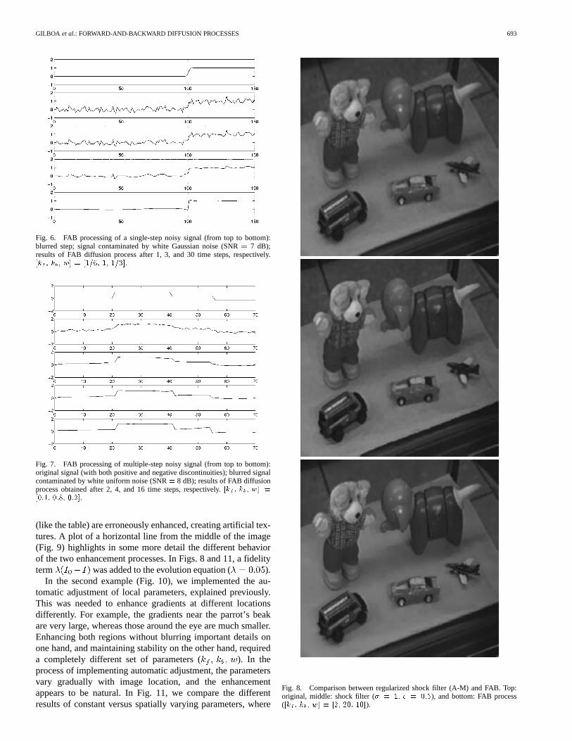
The FAB is also effective in the enhancement of images, as isillustrated in Figs. 8, 10, and 11. In Fig. 8, we compare our re-sults with those obtained by the application of the A-M process[(11)]. The A-M process indeed enhances the objects and formsclear edges, but small details are lost (the teddy bear’s shirt pat-terns, for example). It consequently appears as though the imagehas lost its natural appearance. Also, relatively smooth regions


Fig. 6. FAB processing of a single-step noisy signal (from top to bottom):blurred step; signal contaminated by white Gaussian noise (SNR= 7 dB);results of FAB diffusion process after 1, 3, and 30 time steps, respectively.[k ; k ; w] = [1=6; 1; 1=3].

Fig. 7. FAB processing of multiple-step noisy signal (from top to bottom):original signal (with both positive and negative discontinuities); blurred signalcontaminated by white uniform noise (SNR= 8 dB); results of FAB diffusionprocess obtained after 2, 4, and 16 time steps, respectively.[k ; k ; w] =[0:1; 0:8; 0:2].

(like the table) are erroneously enhanced, creating artificial tex-tures. A plot of a horizontal line from the middle of the image(Fig. 9) highlights in some more detail the different behaviorof the two enhancement processes. In Figs. 8 and 11, a fidelityterm was added to the evolution equation ( ).

In the second example (Fig. 10), we implemented the au-tomatic adjustment of local parameters, explained previously.This was needed to enhance gradients at different locationsdifferently. For example, the gradients near the parrot’s beakare very large, whereas those around the eye are much smaller.Enhancing both regions without blurring important details onone hand, and maintaining stability on the other hand, requireda completely different set of parameters ( ). In theprocess of implementing automatic adjustment, the parametersvary gradually with image location, and the enhancementappears to be natural. In Fig. 11, we compare the differentresults of constant versus spatially varying parameters, where

Fig. 8. Comparison between regularized shock filter (A-M) and FAB. Top:original, middle: shock filter (� = 1; c = 0:5), and bottom: FAB process([k ; k ; w] = [2; 20; 10]).


Fig. 9. Plot of gray level values obtained along one line of Fig. 8: top: original,middle: shock, and bottom: FAB.

(a) (b)

(c) (d)

Fig. 10. FAB diffusion process applied to parrot image, with local parameteradjustment using the MAG measure: Top left: original image, right: blurredimage, and bottom (from left): diffusion process after time steps 1 and 8,respectively.

by using the latter method, the deer, as well as the trees behindthem, are enhanced. We should comment that the process is notsuited too well for the handling of textures, as seen in the spotscreated at the textured ground.

E. Feature-Based Diffusion Coefficient

We further extend and generalize the nonlinear PDE-basedfiltering method, and apply it as a combined feature-basedenhancement and denoising mechanism. In order to avoidsmoothing out important features of the image such as textures,we should ideally have a local feature detector that will slowdown or even reverse the diffusion process in the vicinity ofimportant features.

Fig. 11. FAB diffusion process applied to the deer image. From top: originalimage, result of processing with constant parametersk = 2; k = 50; w =10; magnitude of smoothed gradient of original imageT (x; y) = jrI �G j,(� = 3); result of processing with spatially varying parametersk (x; y) =0:1T; k (x; y) = 6T; w(x; y) = 2T .

We minimize the amount of noise induced by the processing,which is inherently a byproduct of signal enhancement, byour generalized forward-and-backward diffusion processes.Moreover, important features are not filtered out by the forwarddiffusion process, enabling a complementary image processingmechanism to enhance them at a later stage, whenever it isnecessary.

We propose the following general feature enhancing and de-noising mechanism: let


where the local feature estimatorscan be selected from a broad range of choices introduced inthe fields of image processing and computer vision, e.g., edgedetectors (already introduced implicitly under the gradient cri-terion), noise estimators, texture, scale, orientation, curvature,local power-spectrum, moments estimators, etc. The logic dic-tating the value of the diffusion coefficientshould be as fol-lows: Forward diffuse features that should be filtered out be-cause they are corrupted by noise and are of no importance tothe image understanding or appearance. Backward diffuse fea-tures that should be enhanced. Avoid diffusion where either dif-fusion processes (forward or backward) would distort importantfeatures.

In cases where there is somea priori knowledge of the typeof images to be processed, the diffusion process may be muchbetter controlled.

To illustrate this feature-dependent diffusion, consider, forexample, an urban scene, primarily comprised of buildings.In this case, one would like to preserve most vertical andhorizontal lines and edges, significant wall textures and ad-ditional dominant edges at all orientations. To incorporatethese requirements into our diffusion process, let us define bythe symbols the localestimators that stand for edges, wall textures, vertical-lines,and horizontal-lines, respectively. An appropriate diffusioncoefficient for the process is, in this case, given by

(12)

where denotes the relative weight required to balance thedesired effect of each estimator. In this simplified example, itis clear that the diffusion process will slow down considerablywhenever the output of at least one of the weighted estimatorsis much larger than 1 , . In otherareas of the image, a stronger forward diffusion will reduce thenoise.

F. Stability of Smooth Regions in 1-D

Problem definitions:• The flux is defined as follows:

(Note that flux in physical problems is usually definedwith an opposite sign.) We assume a diffusion coefficientof the type , leading to the flux properties

and the antisymmetry relation .• The nonlinear diffusion equation, with its initial and

boundary conditions, is

Fig. 12. Nonmonotonic flux of a forward diffusion process and its criticalpointsM andr.

Lemma 1: If is a local maximum (minimum) inthe spatial domain, then ( ).

Proof:

If is a local maximum, then . Ifis a local minimum, then .

In Theorem 1, we regard the simpler case of positive diffusioncoefficient with nonmonotonic flux. We prove thatonce a gradient gets into the smooth band , where

is the point of maximum flux, it remains trapped there.The maximum of the flux (see Fig. 12) is defined by

Theorem 1 (Smooth Band “Trap”):If, , and , thenfor any .

Proof: Let us assume that at a time we would have. From the continuity of the gradient in time, it

follows that there should be a certain time, ,such that

However, since must be a local maximum, itfollows fromLemma 1that , which contradictsour assumption.

Similarly, the assumption that at time we would havecannot hold.

Theorem 2is the version ofTheorem 1, adapted to our pro-posed FAB coefficient, having both positive and negative valuesof .

The points of extrema of flux, in a FAB diffusion process, aredefined as follows (see Fig. 13):


Fig. 13. Flux and critical points of the FAB process.

This theorem states that, in the 1-D case, a pointwith aninitial gradient magnitude below will not assume a gradientmagnitude larger than (i.e., will stay “smooth”) through theentire forward-and-backward diffusion process, provided theforward maximum flux, , is larger than the backward one,

.Theorem 2 (Stability of Smooth Regions):If , then,

for every for which , the derivative staysbounded at all times, i.e., for any .

Proof: Follows directly from Theorem 1, letting, and . The fact that can also have nega-

tive values does not affect the proof.In the case where , is not guaranteed to be a

local maximum.

G. Analysis of Theorem 2 in the Discrete Case

As the equations are solved numerically, we must first see ifthe theorem holds also in the discrete case. The main property,that we relied on in proving our theorem, is the continuity of thegradient in time, which applies only in the continuous domain.We therefore have to analyze the implications of the discretecase. Starting with the original diffusion equation

we replace the first temporal derivative by the forward differ-ence, with a time step of

[for brevity, we use instead of ]. Assumingis in the positive “smooth band,” that is ,

according to our theorem, it cannot get out of this band in thenext time step, hence the following condition must be satisfied:

(13)

where we regard only the case of positivewithout loss ofgenerality. Replacing the second spatial derivative by the centraldifference with a step , and using the Euler method, thecondition changes to

Assigning , , ,and using the flux bound it is sufficient to prove that

and finally

(14)

In order to maintain numerical stability in any such scheme, theknown CFL bound [6] must be obeyed, i.e., (in the 1-D case)

and therefore we must only ensure that

If is monotonically decreasing in the range(this condition is satisfied by our proposed coefficients

and by other proposed gradient-based nonlinear schemes), it isclear that

Substituting , our proof amounts to showing thesimple relation of

and since for any , we may conclude that thetheorem holds for the discrete case.

Otherwise, if is not monotonically decreasing,(14) provides a bound for the time step.

III. SUPER-RESOLUTION BY THE FAB PROCESS

The FAB diffusion process is useful in applications requiringsimultaneous enhancement and smoothing. We present a simplesuper-resolution (SR) scheme, incorporating two main subsys-tems: an interpolator and an enhancer–denoiser, as shown inFig. 14.

A. Some Background: What is SR?

By SR, we refer to the process of artificially increasing theresolution of an image, using side information about the struc-ture of any specific subset of images or of natural images in gen-eral. The processed image should not only have more pixels, butmore importantly, be characterized by a wider band than that ofthe original image.


Fig. 14. Super-resolution processor.

Most applications of SR use several images obtained fromthe same scene or object, taken from slightly different angles orlocations. After proper registration, a higher resolution imagecan be obtained from the low-resolution images by exploitingthe combined information available at the different sets of sam-pling points. Examples of such SR procedures can be found instudies conducted at NASA on satellite images [4], by Schultzand Stevenson [25] processing a series of movie frames, and by[8].

B. Proposed Scheme: Single Image SR

We elaborate an approach suitable for SR based on a singleimage, similarly to [32]. Instead of using a sequence of videoframes or multiple exposure, we exploit the properties commonto a wide range of natural images. Obviously, there are caseswhere only one image is available, and one would still like toenhance the resolution.

Our assumption is that images can be segmented into regionsfalling into one of the following three categories: smooth areas,edges, and textured regions. At this point, we simplify our modeland consider only images that are not endowed by significanttextural attributes, that is, they can be approximated by piece-wise-smooth segments separated by edges.

The proposed scheme receives a low-resolution image as aninput, with possibly some prior information about the structureof the scene. The processing is executed in two steps. First,the image is interpolated to the new desired size. In our im-plementation, we used cubic B-spline interpolation, but othermethods may also be used. The first step provides good resultsover smooth areas, but edges are smeared. The interpolated im-ages often depict ringing effects, with low spatial oscillations.The purpose of the second processing step is to enhance theedges and denoise the interpolation byproducts. This is accom-plished by using the FAB diffusion process. In our implementa-tion, the parameters were locally adjusted accordingto the mean gradient criterion.

C. Resolution Enhancement—An Example

Consider a narrow-band system, such as a cellular phone, thatpermits the communication of only low-resolution images at areasonable rate. We wish to enhance the resolution of an imageat the receiving end of the communication channel in such away that it will appear as though a high-resolution image wastransmitted over a wideband channel.

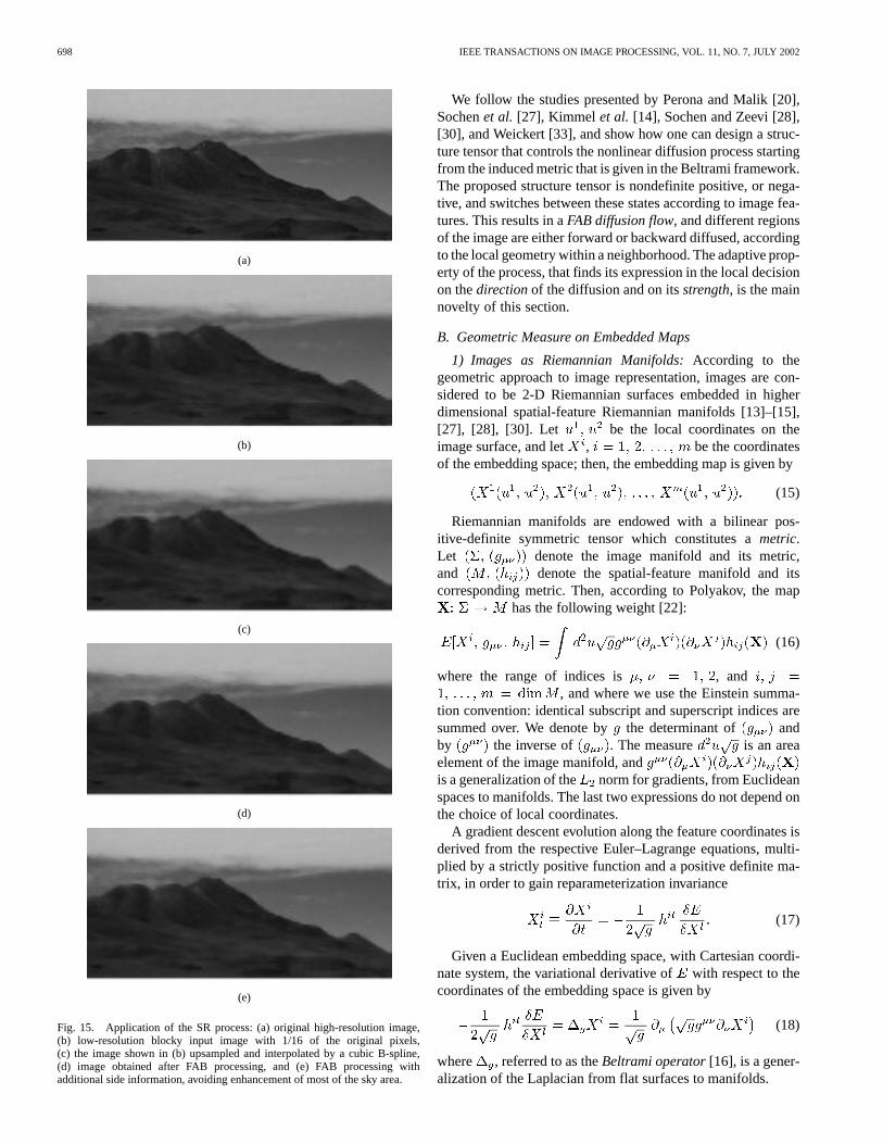
We downsample an input of a high-resolution image by fourin each dimension and send the low-resolution “blocky” image(that is, 1/16 of the original size). At the receiving end, weapply the proposed SR process: the image is up-sampled andenlarged back to its original size. The FAB process is then ap-plied. The end result [Fig. 15(d)] looks more like the originalimage [Fig. 15(a)] than the low-resolution image [Fig. 15(b)].

A considerable improvement can be gained by transmittingsome side information in addition to the image itself. Suchside information may include suitable parameters of theFAB process, specification of segments where enhancementshould be avoided or emphasized, etc. Whenever the originalhigh-resolution image is available at the transmitting end of thechannel, one can find much more easily the optimal parameterssuitable for the task.

In the previous example (Fig. 15), we assumed that additionalinformation was available, specifying where enhancementshould be avoided. Such image segments are typically blurryand fuzzy in the first place, clouds for instance. In Fig. 15(e),we show the result of avoiding enhancement of most of the sky(above a certain horizontal line in the image). This results infuzzy clouds, whereas the mountains below are crisp and sharp.To compare with, in the global enhancement [Fig. 15(d)], theclouds are also sharpened and lose their natural appearance.

We should emphasize here that this resolution enhancementprocess does not come to replace ordinary image compression.It can be used as an additional tool that improves the overallperformance in terms of bandwidth of the final image that isdisplayed. Indeed, the image of Fig. 15(d) [or Fig. 15(e)] is of awider band than that of the transmitted one [Fig. 15(b)].

IV. COLOR PROCESSING

A. Beltrami Framework

The original study of Sochenet al. [27] unifies several ap-proaches by means of the Beltrami framework, and offers newdefinitions and solutions for various image processing tasks.According to the extended Beltrami framework, images, visualobjects, and their characteristics of interest such as derivatives,orientations, texture, disparity in stereo vision, optical flow, andmore, are described as embedded manifolds. The embeddedmanifold is equipped with a Riemannian structure, i.e., a metricthat encodes the geometry of the manifold. Nonlinear operationsare acting on these objects according to the proper local geom-etry. Iterative processes are considered in this context as evolu-tion of manifolds. The latter is a consequence of the action of anonlinear diffusion process or another type of a nonlinear PDE.No global (time-wise) kernels can be associated with these non-linear PDEs. Short time kernels for these processes were derivedrecently in [29] and [40].


(a)

(b)

(c)

(d)

(e)

Fig. 15. Application of the SR process: (a) original high-resolution image,(b) low-resolution blocky input image with 1/16 of the original pixels,(c) the image shown in (b) upsampled and interpolated by a cubic B-spline,(d) image obtained after FAB processing, and (e) FAB processing withadditional side information, avoiding enhancement of most of the sky area.

We follow the studies presented by Perona and Malik [20],Sochenet al. [27], Kimmel et al. [14], Sochen and Zeevi [28],[30], and Weickert [33], and show how one can design a struc-ture tensor that controls the nonlinear diffusion process startingfrom the induced metric that is given in the Beltrami framework.The proposed structure tensor is nondefinite positive, or nega-tive, and switches between these states according to image fea-tures. This results in aFAB diffusion flow, and different regionsof the image are either forward or backward diffused, accordingto the local geometry within a neighborhood. The adaptive prop-erty of the process, that finds its expression in the local decisionon thedirectionof the diffusion and on itsstrength, is the mainnovelty of this section.

B. Geometric Measure on Embedded Maps

1) Images as Riemannian Manifolds:According to thegeometric approach to image representation, images are con-sidered to be 2-D Riemannian surfaces embedded in higherdimensional spatial-feature Riemannian manifolds [13]–[15],[27], [28], [30]. Let be the local coordinates on theimage surface, and let , be the coordinatesof the embedding space; then, the embedding map is given by

(15)

Riemannian manifolds are endowed with a bilinear pos-itive-definite symmetric tensor which constitutes ametric.Let denote the image manifold and its metric,and denote the spatial-feature manifold and itscorresponding metric. Then, according to Polyakov, the map

has the following weight [22]:

(16)

where the range of indices is , and, and where we use the Einstein summa-

tion convention: identical subscript and superscript indices aresummed over. We denote bythe determinant of andby the inverse of . The measure is an areaelement of the image manifold, andis a generalization of the norm for gradients, from Euclideanspaces to manifolds. The last two expressions do not depend onthe choice of local coordinates.

A gradient descent evolution along the feature coordinates isderived from the respective Euler–Lagrange equations, multi-plied by a strictly positive function and a positive definite ma-trix, in order to gain reparameterization invariance

(17)

Given a Euclidean embedding space, with Cartesian coordi-nate system, the variational derivative ofwith respect to thecoordinates of the embedding space is given by

(18)

where , referred to as theBeltrami operator[16], is a gener-alization of the Laplacian from flat surfaces to manifolds.


Assuming an isometric embedding, the image manifoldmetric can be deduced from the mappingand the embeddingspace’s metric

(19)

It is called theinduced metric.2) Metric as a Structure Tensor:There have been a few

studies using anisotropic diffusion processes. Cottet andGermain [5] used a smoothed version of the image to orient thediffusion, while Weickert [34], [35] smoothed also the structuretensor and then manipulated its eigenvalues to steer thesmoothing orientation. Elimination of one eigenvalue from astructure tensor, first proposed as a color tensor in [7], was usedin [24], in which case the tensors are not necessarily positivedefinite. In [33] and [36], the eigenvalues are manipulatedto result in a positive definite tensor. (See also [3], wherethe diffusion is in the direction perpendicular to the maximalgradient of the three color channels; a direction that is differentfrom that of [24].)

We will follow and generalize the analysis elaborated byKimmel et al. in [14]. For completeness, we reiterate some ofthe relations developed in that study. Let us first show that thedirection of the diffusion can be deduced from the smoothedmetric coefficients and may thus be included within theBeltrami framework under the right choice of directionaldiffusion coefficients.

The induced metric is a symmetric positive definitematrix that captures the geometry of the image surface. Letand be the large and the small eigenvalues of , respec-tively. Since is a symmetric positive matrix, its corre-sponding eigenvectors and can be chosen orthonormal.Let , , and therefore

(20)

Let us define

(21)

and

(22)

Our proposed enhancement procedure controls the above de-termined eigenvalues adaptively, so that only meaningful edgesare enhanced, whereas smooth areas are denoised.

C. Adaptive Structure Tensor

1) Controlling the Eigenvalues:From the previous deriva-tion of the induced metric , it follows that the larger eigen-value corresponds to the eigenvector in the gradient direc-tion [in the three-dimensional (3-D) Euclidean case: ].The smaller eigenvalue corresponds to the eigenvector per-pendicular to the gradient direction [in the 3-D Euclidean case:

]. The eigenvectors are equal for both and its in-verse , whereas the eigenvalues have reciprocal values. Wecan use the eigenvalues as a means to control the Beltrami flowprocess. For convenience, let us define . As the

first eigenvalue of (that is ) increases, so does the dif-fusion force in the gradient direction. Thus, by changing thiseigenvalue, we can reduce, eliminate, or even reverse the diffu-sion process in the gradient direction. Similarly, changing

controls the diffusion in the level-set direction.What is the best strategy to control the diffusion process via

adjustment of the relevant parameters? The following require-ments may be considered as guidelines:

• the enhancement should essentially be with relevance tothe important features, while smooth segments should notbe enhanced;

• the contradictory processes of enhancement and noise re-duction by smoothing (filtering) should coexist;

• the process should be as stable as possible, though restora-tion and enhancement processes are inherently unstable.

Let us define as a new adaptive eigenvalue to be con-sidered instead of the original . We propose an eigenvalue thatis a function of the determinant of the smoothed metric. The for-mulation of the new eigenvalue is the same as the FAB diffusioncoefficient, that is

(23)

where is defined by (4) and, here, is chosen to be a func-tion of the smoothed metric: .

2) Algorithm for Color Image Enhancement:To implementthe flow for color image enhancement, we modifyand generalize the algorithm of [14] as follows.

1) Compute the metric . For the channel case (for con-ventional color mapping ) we have

(24)

2) Diffuse the coefficients by convolving them with aGaussian of variance, thereby

(25)

3) Compute the inverse smoothed metric . Change theeigenvalues of the inverse metric , ( ), of

to , respectively. The new second eigen-value should be in the range , preferably min-imal ( ) when the image is not noisy. This yields anew inverse structure tensor that is given by

(26)

4) Calculate the determinant of the new structure tensor.Note that can now have negative values.

5) Evolve the th channel via the Beltrami flow

(27)

Remark: In this flow, we do not get imaginary values, thoughwe have the term , since in cases of negativethe constantimaginary term will be canceled.


3) Comparison to Previous Studies:There are two impor-tant differences between our scheme and that of Kimmelet al.[14, last section]. These concern the possible choice of eigen-values that control the process. As will be illustrated by exam-ples, our choice of eigenvalues may substantially improve thesharpening of natural images.

Let us first return to some analysis of the eigenvalues. Forthe sake of simplicity, we analyze the eigenvalues in the contextof the structure tensor of the smoothed image (insteadof the smoothed structure tensor). We examine (27) for a singlechannel ( ), where and are arbitrary eigenvalues of

. For the degenerate case of , we get . Itcan be shown that for any other than zero, we can write theequation as

(28)

where

where a tilde above any expression indicates that it has beenconvolved with a Gaussian of standard deviation(e.g.,

). For large enough, we can assume the relation, and similarly for the rest of the second derivatives. This re-

lation holds especially at regions of high frequencies—typicallythose image regions containing edges, textures, or noise, as highfrequencies decay exponentially by the Gaussian convolution.Thus, of (28) is small in comparison to the other terms. Theend result is that we get an anisotropic diffusion process with adiffusion coefficient in the direction of the smoothed gradient

and with a different diffusion coefficient,, in the perpendicular direction.This analysis holds for Weickert’s coherence enhancing dif-

fusion, Kimmelet al.’s scheme, and our modification (should not necessarily be constants). It may be concluded at thispoint that controls the measure of directionality of the pro-cesses as follows:

• for small , a close to isotropic diffusion takes place, con-trolled by ;

• for large , a strong anisotropic diffusion occurs and it isbeing controlled by in the smoothed gradient direction,and by in the smoothed level-set direction;

• for constant , the process shifts (accordingto ) from linear forward diffusion to strong coherenceenhancing diffusion;

• for constant , the process shifts fromlinear backward (inverse) diffusion to a Gabor-typeprocess [9], where both processes are unstable.

The relation of anisotropic diffusion, using a tensor diffu-sivity, to Gabor’s idea was mentioned previously in a few studies(such as [14] and [18]), yet, to the best of our knowledge, the re-lation of (28) has not been stated before.

From a numerical viewpoint, the CFL condition in explicitschemes for any (in 2-D) is . There-fore, it is a good practice to limit both eigenvalues to be smallerthan one.

Let us now return to the differences of our scheme to that of[14]. In the latter study, the focus is on the first eigenvalue andon its manipulation. Therefore, the following constraint is pro-posed: . Choosing , onegets . When , the process is completely dom-inated by the second eigenvalue (e.g., for the diffu-sion force in the level set direction is 10times stronger, and thesign of practically does not affect the process). Smoothingalong the level-set lines can be effective in images endowedwith orientational structure, such as those characteristic of fin-gerprints. In general, though, smoothing along level set curveshas the effect of turning nondirectional textures (and noise!) intoartificial zebra-type stripes, which is a drawback for a generalsharpening process. The examples of the Mandrill and Buttonsimages in [14] clearly depict this effect.

Another important property of the present study that ismissing in the one reported in [14] is the adaptive characteristicof the first eigenvalue, implemented in the present study ac-cording to the FAB principles. Whereas in [14] the enhancementis being implemented everywhere, even in smooth regions, theprocess proposed in the present study does it selectively. In ourscheme, the enhancement is directed to locations of edges andsome dominant textures. Global enhancement with a constantnegative causes a considerable noise amplification and thecreation of artificial edges at smooth regions. Examples ofthese phenomena can be found in the experimental results ofthe subsequent Section IV-D.

Regarding stability, for the scheme of [14] behaveslike 2-D inverse diffusion, whereas our scheme behaves like a2-D FAB process (which is much more stable). For large, inregions where the gradient direction stays constant, the schemeproposed in [14] behaves like 1-D inverse diffusion along thisdirection, whereas our scheme behaves like a 1-D FAB process.

D. Experimental Results

We applied three Beltrami-type processes to the Iguana colorimage: the original scheme of [14]; a modified version of [14],where the second eigenvalue is small; and our Beltrami–FABprocess. The results presented in Fig. 16 show that in the firstprocess, smoothing along the edges is very dominant, creatingsnake-like features at places of nonorientational textures (likethe sand). The second process (using a small value of), cre-ates strong sharpening effects but amplifies noise at smooth re-gions (like the sea), as is clearly depicted in the enlargement(Fig. 17). Our Beltrami–FAB process seem to behave well inthis relatively complex natural image.

In Fig. 18, we show the effects of enhancement on a com-pressed image. The Tulip image was highly compressed ac-cording to the JPEG standard. A known byproduct of JPEGcompression is the blocking effects created at smooth regions.Indeed, the original and modified schemes of [14] enhanced the8 8 block boundaries whereas our scheme smoothed them out.

(The color images are available at http://visl.technion.ac.il/ip-fab.)


Fig. 16. Iguana image processed by three Beltrami-type processes. Fromtop: original, scheme of [14] (� = 0:3; � = � ), modified [14]with small � (� = 0:3; � = 0:01), and Beltrami–FAB process(� = � (s); [k ; k ; w; �] = [10; 2000; 1000; 0:5]; � = 0:01). Allprocesses ran 13 iterations,dt = 0:1, � = 2.

V. DISCUSSION ANDCONCLUSIONS

Sharpening and denoising are contradictory requirements inimage enhancement. We show how they can be reconciled bya local decision mechanism that controls the orientation, type,

Fig. 17. Enlargement of a segment of the iguana’s head, with the sea at thebackground. From left: original; image processed by a modification of [14] withsmall� ; and by the Beltrami–FAB. Note that smooth regions like the sea arenot becoming noisy due to processing by our scheme.

Fig. 18. Segment of the compressed tulip image processed by threeBeltrami-type schemes. Top (from left): original; result of processing by thescheme of [14] with� = 0:5; � = � ; processed by a modified [14] withsmall� (� = 0:5; � = 0:1); and processed by the Beltrami-FAB processwith � = � (s); [k ; k ; w; �] = [30; 300; 200; 0:5]; � = 0:1. Allprocesses ran ten iterations,dt = 0:1, � = 1. Note that the JPEG blockingartifacts are not enhanced by the Beltrami–FAB process.

and extent of the diffusion process. The combined FAB diffu-sion process offers practical advantages over previously pro-posed studies in enhancement of image quality.

One of the important aspects of any attempt to implementa truly backward diffusion process in image processing (i.e., aprocess where the diffusion coefficient becomes negative) is theinherent instability. Since the physical diffusion and heat propa-gation occur only as a forward process, the mathematical modelthat well represents the physics becomes ill-posed when the dif-fusion coefficient changes its sign. As is well known, stability isnot well-defined in ill-posed problems. It is therefore importantto take a note of the fact that stability is afforded over certainregimes in the case of the FAB diffusion. We have proven sta-bility for small gradient bands in the 1-D case, and verified thefeasibility of our approach on a variety of signals and images.Intuitively, the stability in the backward process is afforded byits limitation to small areas of very few pixels, surrounded bylarger areas of many more pixels, where the forward diffusionprovides a “safety belt” that avoids explosion. Indeed, since themajority of pixels in natural images are characterized by lowgradients and mainly singular edges give rise to the reversal of


the diffusion coefficient sign, stability is achieved. This argu-ment does not hold any longer when the FAB diffusion processencounters a highly textured or extremely noisy image.

Yet another related facet of the present study is the gener-alization of the framework of the Beltrami flow foradaptiveprocessingof color images. This is accomplished by replacingthe eigenvalues of the color image metric by an adaptive co-efficient that locally controls the orientation and extent of thediffusion. The decision of where and how to adapt the coeffi-cient is based on the edge’s direction and strength, defined bythe eigenvectors and determinant of the smoothed image metric,respectively. FAB diffusion process takes place in the directionof the gradient and forward diffusion takes place in the perpen-dicular direction.

Examples illustrate that this approach works, and that sharp-ening and denoising can be combined together in the enhance-ment of gray-level and color images.

REFERENCES

[1] L. Alvarez and L. Mazorra, “Signal and image restoration using shockfilters and anisotropic diffusion,”SIAM J. Numer. Anal., vol. 31, no. 2,pp. 590–605, 1994.

[2] F. Catte, P. L. Lions, J. M. Morel, and T. Coll, “Image selectivesmoothing and edge detection by nonlinear diffusion,”SIAM J. Numer.Anal., vol. 29, no. 1, pp. 182–193, 1992.

[3] A. Chambolle, “Partial differential equations and image processing,” inProc. IEEE ICIP, vol. 1, 1994, pp. 16–20.

[4] P. Cheeseman, B. Kanefsky, R. Kraft, J. Stutz, and R. Hanson, “Super-re-solved surface reconstruction from multiple images,” inMaximum En-tropy and Bayesian Methods, G. R. Heidbreder, Ed. Norwell, MA:Kluwer, 1996, pp. 293–308.

[5] G. H. Cottet and L. Germain, “Image processing through reaction com-bined with nonlinear diffusion,”Math. Comput., vol. 61, pp. 659–673,1993.

[6] R. Courant, K. O. Friedrichs, and H. Lewy, “On the partial differenceequations of mathematical physics,”IBM J., vol. 11, pp. 215–235, 1967.

[7] S. Di Zenzo, “A note on the gradient of a multi image,”Comput. Vis.,Graph., Image Process., vol. 33, pp. 116–125, 1986.

[8] M. Elad and A. Feuer, “Super-resolution restoration of continuousimage sequence—Adaptive filtering approach,”IEEE Trans. ImageProcessing, vol. 8, pp. 387–395, Mar. 1999.

[9] D. Gabor, “Information theory in electron microscopy,”Lab. Invest., vol.14, no. 6, pp. 801–807, 1965.

[10] G. Gilboa, Y. Y. Zeevi, and N. Sochen, “Anisotropic selective inversediffusion for signal enhancement in the presence of noise,” inProc. IEEEICASSP-2000, vol. I, Istanbul, Turkey, 2000, pp. 221–224.

[11] , “Signal and image enhancement by a generalized forward-and-backward adaptive diffusion process,” inProc. EUSIPCO-2000, Tam-pere, Finland, 2000.

[12] , “Resolution enhancement by forward-and-backward nonlineardiffusion processes,” inProc. Nonlinear Signal and Image Processing,Baltimore, MD, June 2001.

[13] R. Kimmel, N. Sochen, and R. Malladi, “On the geometry of texture,”Berkeley Labs., Univ. California, Berkeley, Rep. LBNL-39640, UC-405,Nov. 1996.

[14] R. Kimmel, R. Malladi, and N. Sochen, “Images as embedding mapsand minimal surfaces: Movies, color, texture, and volumetric medicalimages,”Int. J. Comput. Vis., vol. 39, no. 2, pp. 111–129, Sept. 2000.

[15] R. Kimmel, N. Sochen, and R. Malladi, “From high energy physicsto low level vision,” inFirst International Conference on Scale–SpaceTheory in Computer Vision. New York: Springer-Verlag, 1997, Lec-ture Notes In Computer Science: 1252, pp. 236–247.

[16] E. Kreyszing,Differential Geometry. New York: Dover, 1991.[17] X. Li and T. Chen, “Nonlinear diffusion with multiple edginess thresh-

olds,” Pattern Recognit., vol. 27, no. 8, pp. 1029–1037, 1994.[18] M. Lindenbaum, M. Fischer, and A. Bruckstein, “On Gabor’s contribu-

tion to image enhancement,”Pattern Recognit., vol. 27, no. 1, pp. 1–8,1994.

[19] S. J. Osher and L. I. Rudin, “Feature-oriented image enhancement usingshock filters,” inSIAM J. Numer. Anal., vol. 27, 1990, pp. 919–940.

[20] P. Perona and J. Malik, “Scale–space and edge detection usinganisotropic diffusion,”IEEE Trans. Pattern Anal. Machine Intell., vol.12, pp. 629–639, July 1990.

[21] I. Pollak, A. S. Willsky, and H. Krim, “Scale space analysis by stabi-lized inverse diffusion equations,” inFirst International Conference onScale–Space Theory in Computer Vision. New York: Springer-Verlag,1997, Lecture Notes In Computer Science: 1252, pp. 200–211.

[22] A. M. Polyakov, “Quantum geometry of bosonic strings,”Phys. Lett.,vol. 103B, pp. 207–210, 1981.

[23] E. Radmoser, O. Scherzer, and J. Weickert, “Scale–space properties ofnonstationary iterative regularization methods,”J. Vis. Commun. Image.Represent., to be published.

[24] G. Sapiro and D. L. Ringach, “Anisotropic diffusion of multivalued im-ages with applications to color filtering,”IEEE Trans. Image Processing,vol. 5, pp. 1582–1586, Nov. 1996.

[25] R. R. Schultz and R. L. Stevenson, “Extraction of high-resolutionframes from video sequences,”IEEE Trans. Image Processing, vol. 5,pp. 996–1011, June 1996.

[26] N. Sochen, G. Gilboa, and Y. Y. Zeevi, “Color image enhancement by aforward-and-backward adaptive Beltrami flow,” inAFPAC-2000, LNCS1888, G. Sommer and Y. Y. Zeevi, Eds. New York: Springer-Verlag,2000, pp. 319–328.

[27] N. Sochen, R. Kimmel, and R. Malladi, “A general framework for lowlevel vision,” IEEE Trans. Image Processing, vol. 7, pp. 310–318, Mar.1998.

[28] N. Sochen and Y. Y. Zeevi, “Images as manifolds embedded in a spatial-feature non-Euclidean space,” Technion—Israel Inst. Technol., Haifa,CCIT Rep. 1181, Nov. 1998.

[29] N. Sochen, “Stochastic processes in vision I: From Langevin to Bel-trami,” Technion—Israel Inst. Technol., Haifa, CCIT Rep. 245, June1999.

[30] N. Sochen and Y. Y. Zeevi, “Representation of colored images by man-ifolds embedded in higher dimensional non-Euclidean space,” inProc.IEEE ICIP’98, Chicago, IL, 1998.

[31] B. M. ter Haar Romeny, Ed.,Geometry Driven Diffusion in ComputerVision. Norwell, MA: Kluwer, 1994.

[32] I. Vitsnudel, R. Ginosar, and Y. Y. Zeevi, “Neural network aided designfor image processing,” inProc. SPIE Symp. Visual Communication andImage Processing, vol. 1606, pp. 1086–1091.

[33] J. Weickert, “Coherence-enhancing diffusion of color images,”ImageVis. Comput., vol. 17, pp. 199–210, 1999.

[34] J. Weickert, “Multiscale texture enhancement,” inComputer Analysis ofImages and Patterns; Lecture Notes in Computer Science. New York:Springer, 1995, vol. 970, pp. 230–237.

[35] J. Weickert, “Anisotropic diffusion in image processing,” Ph.D. disser-tation, Kaiserslautern Univ., Germany, Nov. 1995.

[36] J. Weickert, “Scale–space properties of nonlinear diffusion filtering withdiffusion tensor,” Lab. Technomathematics, Univ. Kaiserslautern, Ger-many, Tech. Rep. 110, 1994.

[37] J. Weickert and B. Benhamouda, “A semidiscrete nonlinear scale–spacetheory and its relation to the Perona–Malik paradox,” inAdvances inComputer Vision, F. Solina, Ed. New York: Springer, 1997, pp. 1–10.

[38] R. T. Whitaker and S. M. Pizer, “A multi-scale approach to non uniformdiffusion,” in CVGIP: Image Understand., vol. 57, 1993, pp. 99–110.

[39] A. P. Witkin, “Scale space filtering,” inProc. Int. Joint Conf. ArtificialIntelligence, 1983, pp. 1019–1023.

[40] N. Sochen, “Stochastic processes in vision I: From Langevin to Bel-trami,” in Proc. Int. Conf. Computer Vision, Vancouver, BC, Canada,July 2001, pp. 288–293.

Guy Gilboa received the B.Sc. degree in electricalengineering from Ben-Gurion University, BeerSheva, Israel, in 1997. He is currently pursuingthe Ph.D. degree in electrical engineering at theTechnion—Israel Institute of Technology, Haifa.

He was with Intel Development Center, Haifa, forthree years, working in the design of processors. Hismain research interests are related to variational andPDE-based processes applied to enhancement, sharp-ening, and denoising of images. He is also interestedin computer vision algorithms and their applications

to video surveillance and target recognition.


Nir Sochen received the B.Sc degree in physics in1986 and the M.Sc. degree in theoretical physics1988, both from the University of Tel-Aviv, Tel-Aviv,Israel. He received the Ph.D. degree in theoreticalphysics 1992 from the Université de Paris-Sud,Paris, France, while conducting his research in theService de Physique Théorique, Centre d’EtudeNucleaire, Saclay, France.

He continued with one year of research in the EcoleNormale Superieure, Paris, on the Haute Etude Scien-tifique Fellowship, and a three-year NSF fellowship

in the Physics Department, University of California, Berkeley. It is there thathis interest shifted from quantum field theories and integrable models, related tohigh-energy physics and string theory, to computer vision and image processing.He spent one year with the Physics Department, University of Tel-Aviv, and twoyears with the Faculty of Electrical Engineering, Technion—Israel Institute ofTechnology, Haifa. Since 1999, he has been a Senior Lecturer with the Depart-ment of Applied Mathematics, University of Tel-Aviv. He is also a member ofthe Ollendorf Center at the Technion. His main research interests are the appli-cations of differential geometry and statistical physics in image processing andcomputational vision.

Yehoshua Y. (Josh) Zeevireceived the Ph.D. degreefrom the University of California, Berkeley.

He is the Barbara and Norman Seiden Professorof Computer Science with the Department ofElectrical Engineering, Technion—Israel Instituteof Technology, Haifa. He is the Founder of theJacobs Center for Communication and InformationTechnologies (CCIT) and the Ollendorff MinervaCenter, and served as the Head of those centers. Hewas also the Dean of the Faculty of Electrical En-gineering (1994-1999). He was a Visiting Scientist

at Lawrence Berkeley Laboratory, University of California, Berkeley. He wasa Vinton Hayes Fellow at Harvard University, Cambridge, MA, and has beena regular visitor there. He was also a Visiting Professor at the MassachusettsInstitute of Technology, Cambridge, and Rutgers University, New Brunswick,NJ, and a Senior Visiting Scientist at the NTT Research Center, Yokosuka,Japan. He is presently a Visiting Professor at Columbia University, New York.He is the co-inventor of many patents and the author of over 200 publicationsrelated to vision and image sciences. He is the Editor-in-Chief of theJournal ofVisual Communication and Image Representationand the editor of three books.He is one of the founders of i Sight, Inc., a company that developed digitalvideo cameras that mimic the eye, and UltraGuide, Ltd., a medical technologycompany that develops guidance systems under ultrasound imaging.

Dr. Zeevi is a Fellow of SPIE and the Rodin Academy.

forward-and-backward diffusion processes for adaptive...

Documents