foundation technologies for offshore shallow water … · foundation technologies for offshore...
TRANSCRIPT

Foundation Technologies for Offshore Shallow Water
Renewable Energy Projects
Matthias Laga
Thesis to obtain the Master of Science Degree in
Civil Engineering
Supervisor: Professor Peter John Bourne-Webb
Examination Committee
Chairperson: Prof. Jaime Alberto dos Santos
Supervisor: Prof. Peter John Bourne-Webb
Member of Committee: Prof. Rui Pedro Carrilho Gomes
June 2015
ii

iii
Abstract
Abstract
Bucket foundations have been widely used in oil and gas offshore structures. However, this type of
foundations is also suitable for offshore wind turbines. This dissertation presents the results of a two-
dimensional and three-dimensional finite element analyses of bucket foundations embedded in clay
under undrained conditions, where frictional contact is considered between bucket skirt and subsoil.
Two bucket configurations, solid and shell, are executed and compared with each other. Two soil cases
are modelled, with uniform undrained shear strength and with increasing undrained shear strength.
Aspect ratios L/D for the foundations are taken 0.5, 1 and 2. The performance of a simplified bucket
foundation model under vertical and horizontal load is investigated. The conducted bearing capacities
from FEA are compared with calculated analytical approaches as well as previous studies. It is shown
that FEA agrees well with the analytical approaches and previous studies. Regarding the ultimate
vertical capacity, shell bucket are likely to behave in the same way as solid bucket configurations.
Keywords
Bucket foundation, Finite element analysis, Bearing capacity, Offshore
iv
Acknowledge
Acknowledge
I would like to thank all the people who helped me to achieve the final result of this master dissertation.
Firstly, I would like to thank my supervisor, prof. Peter Bourne-Webb for the opportunity to work on this
master dissertation, for his spent time during several meetings and for his valuable suggestions.
Furthermore, he read my work and helped to improve this dissertation. I am very grateful to him for the
many hours he helped me. Secondly, I would like to thank Lieselot Vantomme, it was a pleasure to work
with her.
Furthermore, I would like to thank my friends in Belgium who were by my side throughout my academic
path for the past 4 years, your unwavering support has been a source of strength and encouragement.
Finally, I would like to give special thanks to my family, in particularly my parents and brother. They
helped and supported me throughout these years of studying in particular during this master dissertation,
which was written abroad.
Thanks to all of you.
Matthias Laga,
June 25, 2015

v
Table of Contents
Table of Contents Abstract ...................................................................................................................... iii
Acknowledge .............................................................................................................. iv
Table of Contents ........................................................................................................ v
List of Figures ............................................................................................................. ix
List of Tables .............................................................................................................. xi
List of Acronyms ........................................................................................................ xii
List of Symbols ......................................................................................................... xiii
1 Introduction .................................................................................................. 15
1.1 Overview ........................................................................................................... 2
1.1.1 Onshore vs. offshore ............................................................................................. 2
1.1.2 Foundations for offshore wind turbine ................................................................... 4
1.2 Motivation and Contents ................................................................................... 5
1.3 Structure of the dissertation .............................................................................. 5
2 Shallow Foundations ...................................................................................... 6
2.1 Introduction ....................................................................................................... 7
2.2 Offshore foundations ......................................................................................... 7
2.2.1 Mono-piles ............................................................................................................. 7
2.2.2 Multi-piles (tripod) .................................................................................................. 8
2.2.3 Gravity base foundations ..................................................................................... 11
2.2.4 Bucket foundation ................................................................................................ 12
2.3 Settlement calculation for shallow foundations .................................................14
2.4 Bearing capacity theory shallow foundation .....................................................16
2.4.1 Conventional bearing capacity ............................................................................ 16
2.4.2 Drained and undrained conditions ....................................................................... 18
2.5 Safety ..............................................................................................................19
2.5.1 Global factors of safety ........................................................................................ 19
2.5.2 Limit state design ................................................................................................. 19
3 Skirt bucket foundation ................................................................................ 22
3.1 Introduction ......................................................................................................23
3.2 Shell bucket components .................................................................................24

vi
3.3 Installation procedure .......................................................................................25
3.3.1 Clayey soils .......................................................................................................... 25
3.3.2 Sandy soils .......................................................................................................... 26
3.3.3 Analytical approach installation in undrained condition ....................................... 26
3.4 Ultimate vertical bearing capacity theory ..........................................................27
3.5 Limit equilibrium solutions vertical pull out capacity..........................................28
3.5.1 Drained response ................................................................................................ 29
3.5.2 Partially drained response ................................................................................... 30
3.5.3 Undrained response ............................................................................................ 31
3.6 Horizontal capacity ...........................................................................................32
3.6.1 Pure horizontal capacity ...................................................................................... 32
3.6.2 Allowance of rotation ........................................................................................... 34
3.7 Previous studies ..............................................................................................35
3.7.1 Le Chi Hung and Sung Ryul Kim (2012) ............................................................. 35
3.7.1.1 Parameters, geometry, boundary conditions and interface ................................. 35
3.7.1.2 Results ................................................................................................................. 36
3.7.2 Yung-gang Zhan and Fu-chen Liu (2010) ........................................................... 37
3.7.2.1 Parameters, geometry, boundary conditions and interface ................................. 37
3.7.2.2 Results ................................................................................................................. 37
3.7.3 H.A. Taiebat and J.P. Carter (2005) .................................................................... 38
3.7.3.1 Parameters, geometry, Boundary conditions and interface ................................ 38
3.7.3.2 Results ................................................................................................................. 38
4 Linear Elatic FEA ......................................................................................... 39
4.1 Introduction ......................................................................................................40
4.2 Solid bucket formation .....................................................................................41
4.2.1 Numerical Model Implementation ........................................................................ 41
4.2.1.1 2D cross section geometry and BC ..................................................................... 41
4.2.1.2 Parameters .......................................................................................................... 42
4.2.1.3 Interaction properties ........................................................................................... 42
4.2.1.4 Mesh .................................................................................................................... 43
4.2.2 Immediate settlement of the solid bucket ............................................................ 44
4.2.2.1 Analytical calculation ........................................................................................... 44
4.2.2.2 Comparison analytical with numerical FE results. ............................................... 45
4.3 Shell bucket .....................................................................................................46
4.3.1 Numerical Model Implementation ........................................................................ 46
4.3.1.1 2D cross section geometry and boundaries conditions ....................................... 46
4.3.1.2 Parameters .......................................................................................................... 47
4.3.1.3 Interaction properties ........................................................................................... 48
4.3.1.4 Mesh .................................................................................................................... 48

vii
4.3.2 Settlement comparison 2D and 3D model ........................................................... 49
4.4 Conclusion .......................................................................................................50
5 Elasto-Plastic FEA ....................................................................................... 51
5.1 Introduction ......................................................................................................52
5.2 Mohr coulomb criterion ....................................................................................52
5.3 Tresca Yield criterion .......................................................................................53
5.4 Two-dimensional analysis ................................................................................54
5.4.1 Numerical model implementation ........................................................................ 54
5.4.1.1 Parameters .......................................................................................................... 55
5.4.1.2 Geometry, boundary conditions, interaction properties and mesh ...................... 57
5.4.2 Shear analysis and results .................................................................................. 58
5.4.2.1 Model Validation .................................................................................................. 58
5.4.2.2 Solid bucket ......................................................................................................... 59
5.4.2.3 Shell bucket ......................................................................................................... 61
5.4.3 Load – Displacement analysis and results .......................................................... 62
5.4.3.1 Analytical calculation of vertical bearing capacity ............................................... 62
5.4.3.2 Results and discussion ........................................................................................ 66
5.5 Three-dimensional analysis .............................................................................74
5.5.1 Numerical Model implementation ........................................................................ 74
5.5.1.1 Parameters .......................................................................................................... 74
5.5.1.2 Geometry, boundary conditions, interaction properties and mesh ...................... 74
5.5.2 Load – Displacement results and discussion ...................................................... 75
5.5.3 Horizontal capacity analysis ................................................................................ 78
5.5.3.1 Analytical results .................................................................................................. 78
5.5.3.2 Results and discussion ........................................................................................ 78
6 Conclusions ................................................................................................. 81
6.1 Summary and Conclusions ..............................................................................82
6.2 Further research ..............................................................................................84
References ............................................................................................................... 85
Appendix................................................................................................................... 89
A. Calculation Moment due to purely horizontal translation of the shell bucket – Vesic Method ...................................................................................................89
B. Settlement calculation solid bucket ..................................................................90
C. Conversion from shell bucket to solid bucket aspect ratio L/D = 1 ....................91
D. Analytical installation calculation undrained conditions ....................................92
E. Calculation of ultimate vertical bearing capacity ...............................................92
F. Calculation for Hult and Mo in soil with uniform strength for different shell bucket aspect ratios ....................................................................................................93

viii

ix
List of Figures
List of Figures
Figure 1-1: Trends EU for onshore and offshore renewable energy projects [4] .......................... 3
Figure 1-2: Share of support structures for online wind turbines in Europe. [4] ............................ 4
Figure 2-1: Mono-pile .................................................................................................................... 7
Figure 2-2: Lateral resistance for bending moments and horizontal loads [8] .............................. 8
Figure 2-3: Multi-pile ...................................................................................................................... 9
Figure 2-4: Tensile, compressive loading and lateral response of multi-piles [26] ..................... 10
Figure 2-5: Jacket support structure with Pile-through-Leg foundation [12] ............................... 10
Figure 2-6: Gravity base structure ............................................................................................... 11
Figure 2-7: monopod (a) and tripod/quadpod (b) ........................................................................ 13
Figure 2-8: settlement behaviour flexible and rigid foundation .................................................... 15
Figure 2-9: Influence factor based on shape, aspect ratio, footing flexibility and depth to a rigid [19] .......................................................................................................................... 15
Figure 2-10: depth correction factor with the charts by [25] for elastic methods with different solid bucket ratios ............................................................................................................ 16
Figure 2-11: Shear stresses based on Terzaghi's soil be bearing capacity theory for strip foundation [27]. ....................................................................................................... 17
Figure 2-12: Skempton’s bearing capacity factor in clay φ = 0 [22] ............................................ 18
Figure 2-13: Eurocode 7 Design Approach [51]. ......................................................................... 21
Figure 3-1: Vertical and horizontal section elevation shell bucket .............................................. 24
Figure 3-2: installation of shell bucket foundation in sand (a) and in clay (b) ............................. 25
Figure 3-3: Analysis of resistance terms for bucket installation in clay ....................................... 27
Figure 3-4: drained condition pull out capacity [29] ..................................................................... 30
Figure 3-5: Partially drained response [29] ................................................................................. 30
Figure 3-6: undrained response uplifting load [29] ...................................................................... 31
Figure 3-7: a) capacity of bucket in soil with uniform strength and with strength proportional to depth no rotation allowed b) mechanism [31]. ........................................................ 32
Figure 3-8: Purely horizontal translation and rotation allowed .................................................... 33
Figure 3-9: a) Capacity of bucket in soil with uniform strength and with strength proportional to depth and rotation allowed b) mechanism [31] ....................................................... 34
Figure 3-10: vertical load-movement curve and capacity according to L/D ratios [40] ............... 36
Figure 3-11: Horizontal load-movement curve and capacity according to L/D ratios [40] .......... 36
Figure 3-12: vertical (a) and horizontal (b) load-displacement curve according different L/D ratios [37]. ......................................................................................................................... 37
Figure 3-13: vertical (a) and horizontal (b) load-displacement curve according different L/D ratios [41]. ......................................................................................................................... 38
Figure 4-1: a) Load-displacement curve and b) stress-strain curve for shallow foundations ...... 40
Figure 4-2: section assignment and dimension properties solid bucket ..................................... 41
Figure 4-3: interaction properties solid bucket elastic model ...................................................... 42
Figure 4-4: Two-dimensional axisymmetric mesh ....................................................................... 43
Figure 4-5 : Three-dimensional axisymmetric mesh ................................................................... 44
x
Figure 4-6: Comparison of analytical and 2D (left) and 3D (right) numerical settlement ratio L/D = 1 .............................................................................................................................. 45
Figure 4-7: section assignment and dimension properties shell bucket ..................................... 47
Figure 4-8: interaction properties shell bucket ............................................................................ 48
Figure 4-9: 3D soil configuration with (a) and without (b) shell bucket ....................................... 49
Figure 5-1: Mohr-Coulomb Failure Criterion ................................................................................ 52
Figure 5-2: Tresca yield criterion ................................................................................................. 54
Figure 5-3: constant undrained shear strength solid bucket (left) and shell bucket (right) ......... 56
Figure 5-4: Undrained shear strength depending on the soil depth for L/D =1 (not to scale). .... 57
Figure 5-5: Numerical displacement-load control shell bucket ratio L/D = 1 ............................... 59
Figure 5-6: Shear stress along the external bucket wall – case 1 .............................................. 60
Figure 5-7: Shear stress along the external bucket wall – Case 2 .............................................. 60
Figure 5-8: Shear stresses along the inner and outer bucket skirt.............................................. 61
Figure 5-9: adhesion factor undrained failure condition [49] ....................................................... 62
Figure 5-10: ultimate vertical bearing capacity of a shell bucket𝐿 .............................................. 64
Figure 5-11: Vertical ultimate bearing capacity .......................................................................... 64
Figure 5-12: General load-displacement graph shell .................................................................. 65
Figure 5-13: Vertical compression bearing capacity solid bucket - Case 1 and 2 ...................... 67
Figure 5-14: Compression bearing capacity shell buckets - Case 1 and 2 ................................. 68
Figure 5-15: Undefromed (transparent) and deformed (green) mesh after displacement of 0.15m - R1 (left) and R2 (right) .......................................................................................... 68
Figure 5-16: Plastic zones for different ratios – Case 1 – displacement of -0.10m (not to scale) ....................................................................................................................... 69
Figure 5-17: Plastic zones for different ratios – Case 2 – displacement of -0.10m (not to scale) ....................................................................................................................... 70
Figure 5-18: Comparison vertical bearing capacity solid and shell bucket - Case 1 & 2 ............ 71
Figure 5-19: Vector displacement after applying a tension load on shell bucket R0.5 with a) no gap configuration and b) gap configuration ............................................................ 72
Figure 5-20: Reverse bearing capacity shell buckets ................................................................. 73
Figure 5-21: System of axes ....................................................................................................... 74
Figure 5-22: Mesh configuration: C3D8 ...................................................................................... 75
Figure 5-23: comparison 2D and 3D analysis ............................................................................. 76
Figure 5-24: Case 1 - Normalized vertical load-displacement curve, bucket with gap ............... 77
Figure 5-25: Comparison normalized ultimate vertical-displacement curve ............................... 77
Figure 5-26: lateral bearing capacity factor Np in function of the aspect ratios L/D ................... 79
Figure 5-27: Normalized horizontal bearing capacity with rotation for different aspect ratios. ... 79
Figure 5-28: Vector displacement failure mechanism under purely horizontal load (a) and horizontal load with rotation (b) for aspect ratio L/D = 2. (not to scale) .................. 80

xi
List of Tables
List of Tables
Table 2-1: overview foundation types application, advantages and disadvantages [24] ............ 13
Table 2-2 (continue): overview foundation types application, advantages and disadvantages [24] ............................................................................................................................. 14
Table 3-1: Model material parameters [40]. ................................................................................ 35
Table 3-2: model material parameters [37]. ................................................................................ 37
Table 4-1: Solid Bucket Aspect ratio L/D = 1 evaluation method settlements comparison (mm) 46
Table 4-2: Shell Bucket Ratio 1 numerical FE settlements (mm)................................................ 49
Table 5-1: Material properties for solid and shell bucket in clay soil for aspect ratio L/D = 1 ..... 55
Table 5-2: Bearing capacity from FEA for solid bucket Case 1 and 2 ........................................ 63
Table 5-3: Analytical compression bearing capacity for shell bucket Case 1 and 2 ................... 65
Table 7-1: Calculation for Hult and Mo in soil with uniform strength for different shell bucket aspect ratios .......................................................................................................................... 93

xii
List of Acronyms
List of Acronyms
ANS
AS
BC
EU
FE
FEA
GBS
NM
OWE
OWT
RS
UF
2D
3D
Average Numerical Settlement
Analytical Settlement
Boundary Condition
European Union
Finite Element
Finite Element Analyses
Gravity Based Structure
Not Mentioned
Offshore Wind Energy
Offshore Wind Turbine
Relatively Settlement
Universal Foundations
Two-Dimensional
Three-Dimensional

xiii
List of Symbols
List of Symbols
ѵ – Poisson’s ratio
ρ – density (𝐾𝑔/𝑚3)
A – Area (m2)
cu – undrained shear resistance (kPa)
D – diameter (m)
Di – inner diameter (m)
Do – inner diameter (m)
E – Young Modulus (kPa)
L – length (m)
𝑞𝑠 – shaft shear resistance (kN/m2)
𝑆𝑖 − Settlement at the corner of a rectangular area (m)
𝑞𝑛 − Net foundation pressure (N/mm2)
𝐵 − Width of the foundation
𝐼𝑓 − Influence factor based on shape, aspect ratio, footing flexibility and depth to a rigid
𝑞𝑓 − Ultimate bearing capacity due to base resistance (N/mm2)
𝑁𝑐, 𝑁𝑞 and 𝑁𝛾 − dimensionless bearing capacity factors
𝑆𝑐 ,𝑆𝑞 and 𝑆𝛾 − dimensionless modification factor for foundation shape, inclination and depth
𝑞𝑏 − vertical stress acting at the elevation of the base of foundations due to the soil (N/mm2)
𝑐 − cohesion of the soil
𝛾 − unit weight of the soil
𝑞𝑜𝑏 − total overburden pressure removed at foundation footing (N/mm2)
𝑞𝑎 − Allowable bearing capacity (N/mm2)
𝐹𝑠 − safety factor
𝑉𝑖𝑛𝑠𝑡𝑎𝑙 − the installation vertical capacity of shell bucket;
𝑠𝑢1 − the average undrained shear strength over (ℎ + 𝑠);
xiv
𝑠𝑢2 − the undrained shear strength at depth (ℎ + 𝑠).
𝐶𝑑 − Value from the charts [19] based on 𝐷
√𝐿𝐵 and
𝐿
𝐵 where 𝐷 is the depth of the footing, 𝐿 and 𝐵 are
respectively length and width of the footing base. (-)
𝜁𝑠 − shape factor f (-)
𝜁𝑑 − embedment factor (-)
𝐻𝑢𝑙𝑡 − ultimate horizontal capacity (kN)
𝑁𝑝 − lateral bearing capacity factor (-)
∅ − friction angle (°)
– Dilatation angle (°)

xv
Chapter 1
Introduction
1 Introduction
This chapter gives a brief introduction to the importance of renewable energy, in particular wind energy.
Because of the ongoing demand for green and efficient energy, developers are searching for cost
efficient methods to establish these wind turbine structures by looking at the foundations. The motivation
and the objectives behind this dissertation are also presented and at the end of the chapter, the thesis
structure is outlined.
2
1.1 Overview
In the last decades more and more energy was needed to fulfill the needs of humankind. Nowadays this
energy comes mainly from petroleum and gas industry. However, it has become clear that our planet
does not have enough petroleum and gas to supply the increasing human energy demand for the next
decades. Where nuclear power seems to be the cheapest and fastest way to produce energy, it has
already been proven that it is not always the safest. The last twenty years discussions were made about
the nuclear waste and it was the nuclear disaster in Fukushima, Japan 2011 that changed the mind of
many civilians and politicians about the realizations of nuclear reactors.
A lot of alternative energy methods have already been established including wind, solar, tidal,
geothermal and biomass. After hydropower, which amounts to 64% of the total renewable power energy
at the end of 2013, wind power follows with 20% [1]. It can be said that the wind energy is now a
mainstream power source and it will be one of the most rising markets of the future.
The European Union (EU) aims to decrease its dependence on imported fossil fuels and make
alternative energy more sustainable. A set of binding targets have been agreed that aim for twenty
percent of energy consumption to be met from renewable sources by the end of 2020 [2]. As this
dissertation is about the foundations for wind turbines, only the wind power will be discussed further.
The greatest advantage of wind power is its clean, non-polluting and not generating waste products in
contrary to fossil fuels. Also, the wind energy in itself is a source that can be produced over and over
again since the availability is plenty. Disadvantages of wind power are the visual impact, noise
disturbances and the periodic shadow of the rotor blades. Another problem of wind energy is the
changing energy supply. Even though wind turbines have certain systems to maximize power production
at a given wind speed and direction, only in some range of wind speeds the installed power will really
be reached [3].
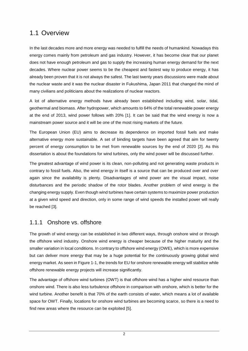
1.1.1 Onshore vs. offshore
The growth of wind energy can be established in two different ways, through onshore wind or through
the offshore wind industry. Onshore wind energy is cheaper because of the higher maturity and the
smaller variation in local conditions. In contrary to offshore wind energy (OWE), which is more expensive
but can deliver more energy that may be a huge potential for the continuously growing global wind
energy market. As seen in Figure 1-1, the trends for EU for onshore renewable energy will stabilize while
offshore renewable energy projects will increase significantly.
The advantage of offshore wind turbines (OWT) is that offshore wind has a higher wind resource than
onshore wind. There is also less turbulence offshore in comparison with onshore, which is better for the
wind turbine. Another benefit is that 70% of the earth consists of water, which means a lot of available
space for OWT. Finally, locations for onshore wind turbines are becoming scarce, so there is a need to
find new areas where the resource can be exploited [5].

3
The installation cost of offshore turbines is likely to be 40% higher than equivalent onshore wind turbines.
The design cost is also higher because of the harsher environmental loads and conditions on the
foundations, tower and turbine itself. Although they are more expensive, these structures provide greater
capacity and higher potential development compared to onshore wind turbines. This is due to the
installations being taller and to accommodate longer blades, which leads to a larger swept area and so
a higher electricity output [6].
However, the most obvious difference between onshore and offshore wind farms is the more significant
support and foundation requirement for OWT. Approximately 40% of the cost of a turbine lies in the
foundation support [6] and because of these higher costs, engineers are trying to find cost-efficient ways
to produce foundation types for these wind turbines. Because companies already gain more than ten
years of experience, the major challenge now is to reduce the development cost by finding alternative
foundations concepts.
As the size and capacity of wind turbines grows, the total weight of the whole structure and the lateral
loads due to outside forces will also increase. That is why the foundation plays a significant role in the
construction of the OWT.
At the end of 2014, a total amount of 2,920 support structures were fully installed in European offshore
wind farms. It should be noted that a support structure is not the same as the foundation. The support
structure is the connection between tower and foundation, thus it can comprise the foundation and its
method of fixing the seabed. In the Figure 1-2, a percentage of each type of support structure is shown.
At present, the commonly used type for OWT installed in shallow waters, where the water depths usually
Onshore
Offshore
Figure 1-1: Trends EU for onshore and offshore renewable energy projects [4]
4
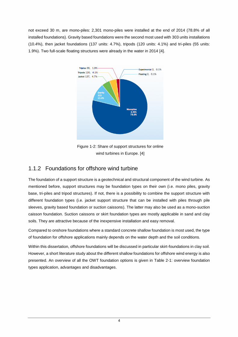
not exceed 30 m, are mono-piles: 2,301 mono-piles were installed at the end of 2014 (78.8% of all
installed foundations). Gravity based foundations were the second most used with 303 units installations
(10.4%), then jacket foundations (137 units: 4.7%), tripods (120 units: 4.1%) and tri-piles (55 units:
1.9%). Two full-scale floating structures were already in the water in 2014 [4].
1.1.2 Foundations for offshore wind turbine
The foundation of a support structure is a geotechnical and structural component of the wind turbine. As
mentioned before, support structures may be foundation types on their own (i.e. mono piles, gravity
base, tri-piles and tripod structures). If not, there is a possibility to combine the support structure with
different foundation types (i.e. jacket support structure that can be installed with piles through pile
sleeves, gravity based foundation or suction caissons). The latter may also be used as a mono-suction
caisson foundation. Suction caissons or skirt foundation types are mostly applicable in sand and clay
soils. They are attractive because of the inexpensive installation and easy removal.
Compared to onshore foundations where a standard concrete shallow foundation is most used, the type
of foundation for offshore applications mainly depends on the water depth and the soil conditions.
Within this dissertation, offshore foundations will be discussed in particular skirt-foundations in clay soil.
However, a short literature study about the different shallow foundations for offshore wind energy is also
presented. An overview of all the OWT foundation options is given in Table 2-1: overview foundation
types application, advantages and disadvantages.
Figure 1-2: Share of support structures for online
wind turbines in Europe. [4]

5
1.2 Motivation and Contents
This work aims to fill some gaps regarding the understanding of the vertical and horizontal behaviour of
skirt bucket foundations with different aspect ratios, in conjugation with other past investigations. The
ultimate goal is to gain a complete understanding of the effect of mechanical loads on the foundation
element. In order to achieve this goal, numerical analysis of this foundation was performed with
ABAQUS and the results are reported and discussed in this dissertation.
In order to become these numerical results, two geo-models were conducted. First, a completely elastic
model was executed where analytical results are compared with numerical outcomes. Secondly, a linear
elastic perfectly plastic Tresca model was performed in order to compare gained results with analytical
calculations and previous studies.
This dissertation can also be seen as a step-by-step plan in order to become a fully operational finite
element shell bucket model. In each case, clarifications for both models were listed at the beginning of
the chapter.
1.3 Structure of the dissertation
This thesis is composed of six main chapters which are ordered as follow:
1. Chapter 1: Introduction;
2. Chapter 2: Shallow foundations;
3. Chapter 3: Skirt-bucket foundation;
4. Chapter 4: Elastic model
5. Chapter 5: Tresca Model;
6. Chapter 6: Conclusions.
In Chapter 1, a general overview of the renewable energy sector and the increase of importance is
given. Chapter 2 and 3 constitute the literature review of the dissertation, where an overview of currently
wind turbine foundation types is given. Also theoretical approaches were given and explained in order
to apply them in following calculations. In Chapters 4 and 5, the elastic and Tresca analysis respectively
are presented using the finite element program ABAQUS. The numerical models used to perform these
analyses are described and then the results are detailed discussed. Finally, in Chapter 6, a summary of
the most pertinent results is presented and conclusions are drawn.

6
Chapter 2
Shallow foundations
2 Shallow Foundations

7
2.1 Introduction
This chapter reviews with the application of offshore foundations for wind turbines. First a brief overview
of offshore foundations types is given. Afterwards soil characteristics for each typical foundation type
will be explained and subsequently the design methods for the prediction of the settlement and bearing
capacity for the shallow foundations will be executed.
2.2 Offshore foundations
The first offshore well dates back to the 19th century, so companies have already gained a lot of
experience in this particular field. It seems that foundations for OWT could easily be designed based on
the design principles of the gas and oil industry. However, this is only partially true. The dominant loading
of an offshore gas- or oil structure is typically from lateral loading from waves and the vertical weight of
the platform, whereas for OWT, lateral loads due to wind and waves remain high while the vertical weight
is low. Horizontal and moment loads from wave and wind action play a significant part in the analysis of
the total OWT system [7, 8]. The different types of foundations applicable for OWT are discussed below
and thereafter a summary of applications, advantages and disadvantages is given in Table 2-1.
2.2.1 Mono-piles
The most common support structure and foundation type for OWT is, due to its relatively simple design
and easy installation, a mono-pile. As seen in Figure 2-1, the support structure is directly connected to
the tower or through a transition piece.
d
Support structure /
Foundation
Transition piece
Figure 2-1: Mono-pile

8
The structure consists of a large diameter cylindrical steel pile driven into the seabed. Depending on the
soil next to the foundation, the steel pile is rammed into the sea floor using hammering or vibration to a
depth of 35 m to 40 m. The diameter of the mono-pile ranges from 3 to 6 m and the wall thickness can
be as high as 150 mm. This type of foundation is an attractive concept in shallow water if the external
conditions are suitable, this means the soil profile must consist of fine or medium dense materials (sand
and clay).
Increasing the capacity of the wind turbine, larger vertical loads will occur through the increased weight
of the nacelle, blades, tower and support structure. The pile foundation must be able to transfer all
vertical loads to the seabed. This is mainly done by friction between the soil and the pile. For mono-
piles, large bending moments and horizontal loads due to wind and wave must also be transferred
directly to lateral resistance of the foundation, Figure 2-2.
Regarding the foundation, scour protection is installed on the seabed to prevent scour or erosion holes.
Near the mono-pile, the current flow and wave action will be stronger than in open sea, which disturbs
the area around the mono-pile causing erosion holes. The seabed layer has a tendency to be reduced
and therefore, the length of the mono-pile exposed to hydrodynamic loads increases. First a layer of
small rock / quarry run is dumped acting as a filter, and then the second larger stone layer is installed
above the first one [9].
2.2.2 Multi-piles (tripod)
The main support structure is a cylindrical steel tube that extends into the tower and the lower part
consists of braces and legs, as seen in Figure 2-3. In each corner of the tripod the substructure is fixed
to the seabed using piles installed through sleeves. The legs are connected to the main cylindrical tube
making the transition with the tower. In contrast to a mono-pile, this type does not require any special
seabed preparations or scour protection [10].
Figure 2-2: Lateral resistance
for bending moments and
horizontal loads [8]

9
`
The diameter of each pile is less than a single mono-pile and varies between approximately 3 m and
3.5 m. The hydrodynamic loads on each pile will be lower and because of the larger base, the structure
will be stiffer. Multi-pile structures are designed for water depths from 25 m to 50 m [11].
It has to be noticed that the multi-pile configuration is also applicable for lattice or jacket structures.
These support structures are commonly used as a fixed offshore platform in gas- and oil industry but
can also be used for OWT. A simple configuration only provides one pile in each corner of the jacket,
Figure 2-5. These steel welded piles are also driven through and eventually grouted to the pile
guides/sleeves in the corner of the jacket [12]. Piles are installed to resist the deadweight of the structure
and to withstand large overturning moments. The latter is transferred to the ground due to the large base
area of the foundation.
In both configurations, tripod or lattice structure, the overall load transmission is different than mono-
piles. Multi-piles are often subjected to both tensile and compressive loading and also subjected to
lateral response. As seen in Figure 2-4, overturning moments are converted to pairs of forces and
transferred as axial loads into the soil. This can be an improvement especially in weak soils, with respect
to the greater friction surface of the different piles, compared to a mono-pile.
d
Figure 2-3: Multi-pile

10
Two different types of pile installation are possible, driven and grouted piles. The most commonly used
for offshore structures are driven piles because of their reliability and easy construction path.
Driven piles: Pile diameter varies among 0.76 m to 2.5 m, but exceptionally a diameter of 5.1 m has
already been used for OWT in the North Sea. The wall thickness of the pile will vary
along the length. Near the pile head, bending moments are always at their maximum,
which results in thicker walls. Another advantage of this type is the exclusion of the
corrosion problem, as the steel pile embedded in the seabed has no contact with oxygen
[13]. The piles can also be inclined to withstand higher loads.
Grouted piles: Grouted piles comprise a steel tubular pile inserted into an oversized pre-drilled hole,
which is filled with grout.
In uncemented sediments, the grout pressure acts to maintain the lateral pressure
between the pile and the surrounding soil, ensuring shaft resistance is mobilized. In
cemented sediments and rocks, it is the strength of the pile-soil bond that ensures the
capacity. Where the seabed consists of calcareous sediments and other potentially
crushable materials, grouted piles are more reliable than driven piles because they do
not degrade the foundation soil [13].
Because of the higher cost, long construction period and the high amount of wind
turbines in a wind farm, this type of pile is inefficient and not considered as an OWT
foundation.
Figure 2-4: Tensile, compressive
loading and lateral response of
multi-piles [26]
Figure 2-5: Jacket support structure with
Pile-through-Leg foundation [12]

11
2.2.3 Gravity base foundations
The gravity base structure, Figure 2-6, can be seen as support structure and foundation together.
Shallow footings are designed to be founded at or just below the seafloor, transferring the loads to the
ground. Since 1990, it has been the second most common foundation type for OWT. In its earliest
application to OWT, the GBS consisted of solid concrete to grant stability to the wind turbine. Nowadays,
they consist of reinforced and pre-stressed concrete but also examples constructed from steel and
hybrid structures of concrete and steel exist.
Regarding transportation, these structures are heavy and difficult to install on site. To eliminate this
particular problem, GBS are made hollow and subsequently filled with ballast material to obtain the full
design weight. The main advantage of this foundation type is the reduced amount of steel and cost, also
as a result of the increased steel prices. This type of foundation has been developed for the construction
of the Thornton Bank Offshore Wind Farm, located 30 km off the Belgian Coast. Here the deepest
registered offshore wind farm with gravity-based structures has a water depth up to 27 m [15].
Offshore GBS are typically larger than onshore configurations because the larger deadweight of wind
turbines and the harsher environmental conditions. The main disadvantages are the construction time
and the need for dredging to level the seabed, placement of a foundation bed filter and gravel layer.
Soil liquefaction of the saturated or partially saturated, loose (low density or compacted), sandy soil
beneath the foundation, due to short repeatedly (e.g. earthquake shaking, storm wave…) or cyclic wave
loading, is an issue that needs to be considered in the design and stability of the structure. These soils
consist of particles that have the tendency to compress when a load is applied. On the other hand,
compressed soil has the tendency to swell (dilatation). In water-saturated soil, the pore spaces between
d
Figure 2-6: Gravity base structure

12
soil grains can be filled with water. Eventually, due to the compaction of the ground, the water pressure
will tend to flow out of the ground. If the applied load is strongly and repeatedly, the soil will not have
time to drain before another loading takes place. Therefore, the water pressure will increase and exceed
the contact stresses between grains of soil that keeps them together. The soil will lose its shear strength
and eventually behaves like a liquid. Subsequently, failure of the soil will occur and the foundations will
be subjected to large displacements.
That is why cyclic shear test are sometimes carried out to predict the accumulation of excess pore water
pressures. If the water pressures becomes too high, a passive drainage system can be provided in the
base slab to facilitate dissipation of excess pore water pressures [16]. Skirt variants can be added to the
footings of the structure in order to suit the seabed soil conditions.
2.2.4 Bucket foundation
One of the most promising solutions for shallow water OWT are bucket foundations. Unlike GBS, this
foundation type is a light-weight structure equipped with skirts of significant length. This type of
foundation finds its origin in the suction anchors used for floating tension leg platforms in the oil – and
gas industry.
If the support structure is founded on one bucket, as shown Figure 2-7 (a), the foundation is known as
a monopod. Other structures, like jackets, utilizing groups of three or four bucket foundations are called
tri-pod and quad-pod, Figure 2-7 (b). Bucket foundations can resist outside short-term environmental
forces due to the foundation weight, embedment of the skirts and suction. In particular, the ability to
create negative pore water pressure under severe loading, which can is also called “passive suction”
[17]. Active suction, in contrary, is a used to install the foundation bucket. This type of foundation is
typically installed in soil with low permeability or low hydraulic conductivity (clay) due to small grain sizes
with large surface areas, which also results in increased friction between soil and structure. However,
also installation in sand is possible with adjustments to the skirts (i.e. water injectors). Further
information of this type of foundation can be found in chapter 5.
As mentioned before, the majority of offshore wind foundations are mono-piles and gravity based
foundations. Future projects will be installed at greater depths where wind conditions are better so tripod
or quadpod foundations with jacket support structures may become more practicable. In December
2002, a full scale prototype of a monopod was installed in Fredrikshavn (Denmark). This five-year
research program showed that the novel principle of a bucket foundation is feasible in suitable soil
conditions (clay or sand) and in water depths up to approximately 40 m [18]. However, another test of a
full-scale prototype monopod structure at Wilhelmshaven (2005) failed during installation because the
skirts started to buckle. This was due to an incorrectly designed wall thickness and stiffener [17].

13
Table 2-1: overview foundation types application, advantages and disadvantages [24]
Foundation Type/
concept
Application advantages disadvantages
Mono-piles Most conditions,
preferably shallow
water and not deep
soft material. Up to 4
m diameter.
Simple, light (minimal
material use) and
versatile. Quick
installation and
minimize construction
risk. Depths up to 35
à 40 m in perfect
environmental
conditions.
Expensive installation
due to large size. May
require pre-drilling a
socket. Difficult to
remove. Large scour
protection required.
Fabrication limits due
to transportation limits
Multiple-piles
(tripod) and lattice
structure
Most conditions,
preferably not deep
soft material.
Applicable for water
depth above 25 to
50m.
Very rigid and
versatile. A lot of
experience from oil
and gas industry
Very expensive
construction and
installation. Difficult to
remove. May require
pre-drilling a socket.
Grouting in pile
sleeves necessary
Concrete gravity
base
Almost all soil
conditions.
Easy transportation
by floating
Expensive due to
large weight
Figure 2-7: monopod (a) and tripod/quadpod (b)

14
Table 2-2 (continue): overview foundation types application, advantages and disadvantages [24]
2.3 Settlement calculation for shallow foundations
Using the elastic theory for immediate settlements under applied stress, qn , the settlement for the corner
of a rectangular flexible foundation may be calculated with Equation 2-1.
𝑆𝑖 = − 𝑞𝑛 𝐵
𝐸 (1 − 𝜈2) 𝐼𝑓 (Equation 2-1)
Where
𝑆𝑖 = Settlement at the corner of a rectangular area
𝑞𝑛 = 𝐹
𝐴=
𝐹
(𝐷
2)2𝜋
Where F is the concentrated force and A the plane area of the footing
𝐵 = Width of the foundation
𝐸 = Young’s modulus of the soil
𝜈 = Poisson’s ratio of the soil
𝐼𝑓 = Influence factor based on shape, aspect ratio, footing flexibility and depth to a rigid
Foundation Type/
concept
Application advantages disadvantages
Steel gravity base Virtually all soil
conditions. Deeper
water than concrete
Lighter than concrete.
Easier transportation
and installation.
Lower expense since
the same crane can
be used as for
erection of turbine.
Costly in areas with
significant erosion.
Requires a cathodic
protection system.
Costly compared with
concrete in shallow
waters.
Mono-suction
caisson
Sands, soft clays. Inexpensive
installation. Easy
removal.
Installation proven in
limited range of
materials
Multiple-suction
caisson (tripod)
Sands and soft clays.
Deeper water.
Inexpensive
installation. Easy
removal.
Installation proven in
limited range of
materials. More
expensive
construction

15
As seen in Figure 2-8, settlement in the center of the flexible foundations will be greater than these on
the corner. This difference is calculated with the influence factor If . In many practical problems the
foundation will be seen as rigid and the settlement is more or less uniform over the area of contact
between the soil and the foundation footing. In order to become a uniform settlement with a flexible
foundation, the contact stresses must increase at the corner and decrease at the center of the
foundation. As seen in Figure 2-9, it can be said that the average settlement of both, center and corner
settlement for flexible foundations will approximately be the same as the uniform settlement of a rigid
foundation.
Equation 2.1 can be modified to include the embedment factor of the foundation. So that the calculation
of analytical immediate settlement for elastic soil models is possible by the use of equations in [25] for
the influence factor and charts [25] for the embedment, H of the shallow foundation. Note that because
of the use of the linear elastic theory no yield point to the plastic behavior will ever occur during the load-
displacement curve. Detailed calculations for settlements after applying a load can be found in Chapter
4. The formula of the immediate settlement can now be determined by:
𝑆𝑖 = − 𝑞𝑛 𝐵
𝐸 (1 − 𝜈2) 𝐼𝑓𝐶𝑑 (Equation 2-2)
Rigid foundation
𝑞𝑛
Soil Flexible foundation
Figure 2-8: settlement behaviour flexible and rigid foundation
Figure 2-9: Influence factor based on shape, aspect ratio, footing flexibility and depth to a
rigid [19]
16
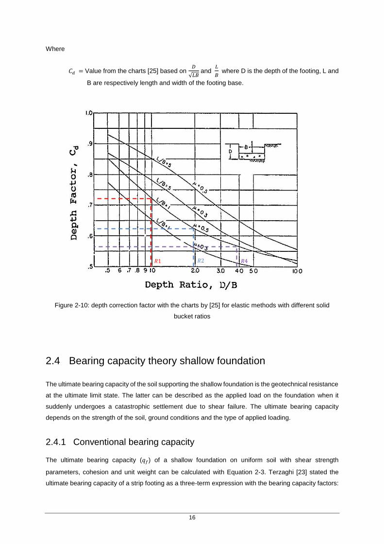
Where
𝐶𝑑 = Value from the charts [25] based on 𝐷
√𝐿𝐵 and
𝐿
𝐵 where D is the depth of the footing, L and
B are respectively length and width of the footing base.
2.4 Bearing capacity theory shallow foundation
The ultimate bearing capacity of the soil supporting the shallow foundation is the geotechnical resistance
at the ultimate limit state. The latter can be described as the applied load on the foundation when it
suddenly undergoes a catastrophic settlement due to shear failure. The ultimate bearing capacity
depends on the strength of the soil, ground conditions and the type of applied loading.
2.4.1 Conventional bearing capacity
The ultimate bearing capacity (𝑞𝑓) of a shallow foundation on uniform soil with shear strength
parameters, cohesion and unit weight can be calculated with Equation 2-3. Terzaghi [23] stated the
ultimate bearing capacity of a strip footing as a three-term expression with the bearing capacity factors:
𝑅1 𝑅2 𝑅4
Figure 2-10: depth correction factor with the charts by [25] for elastic methods with different solid
bucket ratios
17
𝑁𝑐, 𝑁𝑞 and 𝑁𝛾 which are related to the shearing resistance (𝜑). Later on, dimensionless modifications
factors were added for the foundation shape, inclinations and depth.
𝑞𝑓 = c ∙ 𝑁𝑐 ∙ 𝑆𝑐 + 𝑞𝑏 ∙ 𝑁𝑞 ∙ 𝑆𝑞 +1
2 γ ∙ B ∙ 𝑁𝛾 ∙ 𝑆𝛾 (Equation 2-3)
Where
𝑞𝑓 = Ultimate bearing capacity due to base resistance
𝑁𝑐, 𝑁𝑞 and 𝑁𝛾 = dimensionless bearing capacity factors
𝑆𝑐 ,𝑆𝑞 and 𝑆𝛾 = dimensionless modification factor for foundation shape, inclination and depth
𝑞𝑏 = vertical stress acting at the elevation of the base of foundations due to the soil
B = foundation width
𝑐 = cohesion of the soil
𝛾 = unit weight of the soil
Equation 2-3 expresses the general shear failure as the sum of shear resistance. The first term is related
to the cohesion of the soil. The second term is related to the depth of the footing and the overburden
pressure or vertical stress 𝑞𝑠 and the third term is related to the width of the footing and the length of
the shear stress area. All dimensionless bearing capacity factors are related to the angle of shearing
resistance [20, 21].
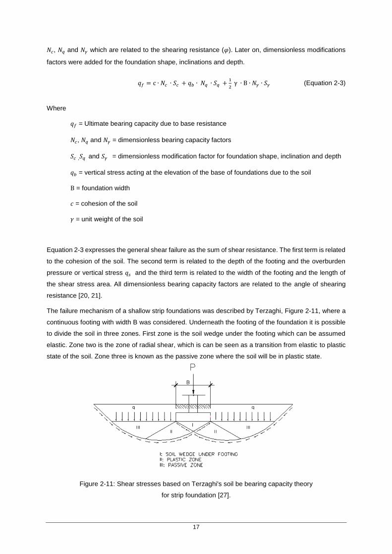
The failure mechanism of a shallow strip foundations was described by Terzaghi, Figure 2-11, where a
continuous footing with width B was considered. Underneath the footing of the foundation it is possible
to divide the soil in three zones. First zone is the soil wedge under the footing which can be assumed
elastic. Zone two is the zone of radial shear, which is can be seen as a transition from elastic to plastic
state of the soil. Zone three is known as the passive zone where the soil will be in plastic state.
Figure 2-11: Shear stresses based on Terzaghi's soil be bearing capacity theory
for strip foundation [27].

18
2.4.2 Drained and undrained conditions
For drained conditions (long-term), the calculations are done in terms of the effective stress where 𝜑’ is
greater than 0 and the three bearing capacity factors Nc, Nq and N are also greater than 0. The long-
term stability of the shallow foundation can now be calculated with c equal to the effective cohesion c’
and 𝜑’ equal to the effective angle of shearing resistance. For drained conditions, qs is equal to the
vertical effective stress and so will be influenced by the position of the groundwater level.
For undrained loadings (short-term), the calculations can be done in terms of the total stress in the soil.
The short-term stability of a shallow foundation can be calculated by taking the cohesion equal to the
undrained shear strength su , Nq = 1 and N = 0. In undrained conditions, qs will be equal to the vertical
total stress at the base of the foundation [23].
Equation 2-3 is now simplified to equation 2-4 which is widely used for undrained clay soils:
𝑞𝑓 = 𝑠𝑢 ∙ 𝑁𝑐𝑢 + 𝑞𝑠 (Equation 2-4)
Where Ncu = Nc.sc.dc is Skempton’s bearing capacity factor where dc = factor. The shape factor of the
foundations can be sequentially calculated with:
𝑆𝑐 = 1 + 0.2 ∙ (𝐵 𝐿⁄ ) for B ≤ L (Equation 2-5)
It should be noticed that the exact theoretical solutions for the depth factor are not available therefore
the magnitude of the depth factor is often based on semi-empirical correlations. The Skempton’s bearing
capacity factor can also be obtained from Figure 2-12.
Figure 2-12: Skempton’s bearing capacity factor in clay φ =
0 [22]

19
2.5 Safety
2.5.1 Global factors of safety
Calculations for the design of an offshore structure must incorporate a factor of safety. The ultimate
bearing load which a foundation can withstand may be calculated using the conventional bearing
capacity theory. In order to calculate the allowable bearing load on the structure a safety factor must be
applied. Definitions are explained below:
Ultimate bearing capacity (qf) : is the value of bearing stress which causes a sudden catastrophic
settlement of the foundation due to shear failure.
Allowable bearing capacity (qa): is the maximum bearing stress that a foundation can support in order
to have allowable settlements and remain safe against instability due to failure. The allowable bearing
capacity is calculated from the ultimate bearing capacity using a factor of safety (FS) as seen in equation
2-7 [23].
Net ultimate bearing pressure (qnet,f) where the ultimate bearing capacity is the total stress that can be
applied at the footing of the foundation, stresses from the overburden pressure at the foundation level
also contribute the bearing failure. The net bearing capacity qnet,f can then be expressed as Equation
2-6.
𝑞𝑛𝑒𝑡,𝑓 = 𝑞𝑓
− 𝑞𝑜𝑏
(Equation 2-6)
Where
𝑞𝑜𝑏 = γ ∙ 𝐷𝑓 = total overburden pressure removed at foundation footing
Notice that no bearing failure of the soil will ever happen if the applied load is equal to the total
overburden pressure.
𝑞𝑎 = 𝑞𝑛𝑒𝑡,𝑓
𝐹𝑠+ 𝑞
𝑜𝑏 (Equation 2-7)
The factor of safety in soft clay soils is likely to be 2.5. In stiff clay FS is taken around 3.0 because
settlements can be quite high even though the ultimate bearing capacity in these soils is relatively large.
Traditionally, a global factor of safety approach such as this would have been used. However most
current design standards not use a limit state approach, as described in the following section.
2.5.2 Limit state design
Skirt bucket foundations with same dimensions as GBS shall be considered as GBS for conditions after
the installation is completed. The skirts will penetrate into the ground and compress the soil plug inside
bucket acting as a solid foundation. This means that limit state design from GBS can be applied to skirt
foundation [48]. To ensure the stability of these foundations, shear failure below the footing of the
structure will be investigated. This includes the failure along any potential shear surface with

20
considerations to the cyclic loading effect on the foundation and the effect of soft layers in the ground.
These analyses are conducted for drained, partially drained or undrained conditions whatever suits most
to the actual soil condition.
Requirements based on Limit state method of design are necessary to assure safety of the structure.
Two different limit states are applicable, ultimate limit state (ULS) and accidental limit state (ALS). To
evaluate the stability of these structures, two different analysis are possible:
Effective stress stability analysis based on effective strength parameters of soil and
estimations of the pore water pressure;
Total stress stability analysis based on total shear strength parameters.
The safety against overturning of the structures is investigated with ULS and ALS. The stability of the
overall structure will be analysed in ULS by application of the material factors to the characteristic soil
shear strength parameters:
γM = 1.15 for effective stress analysis
= 1.25 for total stress analysis
In Figure 2-13, the basic design approach by Eurocode 7 for offshore foundation is given. It can be seen
that the partial material factors mentioned above are about 10 % smaller than those specified in
Eurocode 7 [51].
It is also important to take a closer look to the Serviceability Limit State (SLS). Serviceability criteria will
define tolerance requirements for the operation of the OWT.
Serviceability limit state (SLS) for offshore steel structures can be associated with [48].:
Vibrations in the steel structure that may discomfort the maintenance person;
Deflections which may prevent the intended operation of equipment
Deflections which may be detrimental to finishes or non-structural elements deformations
Deflections which may spoil the aesthetic appearance of the structure
Serviceability limit state (SLS) design conditions, analyses of settlements and displacements have to be
calculated in terms of [48]: Initial consolidation and secondary settlements; differential settlements;
permanent (long term) horizontal displacements; dynamic motions.
Typically these tolerances are specified in guidelines, i.e. DnV. Some of the specified requirements are
[52]:
Max. allowable rotation at foundation head after installation. DnV code specifies 0.25 degree
limit on “Tilt” at the nacelle level;
Maximum accumulated permanent rotation resulting from cyclic and dynamic loading over the
design life.

21
Figure 2-13: Eurocode 7 Design Approach [51].
22
Chapter 3
Skirt bucket foundation
3 Skirt bucket foundation

23
3.1 Introduction
Since early 1980’s, skirt-bucket foundations or suction caissons have been used as anchors for floating
platforms in the offshore oil- and gas industry. The suction bucket is a steel, cylinder-shaped upturned
structure that is embedded in the seabed and is closed at the top. In most cases embedment is achieved
by self-weight, by pushing the caisson skirts downwards and by creating negative pressure inside the
caisson skirt. Skirt-friction and end bearing will occur after removal of the pump keeping the foundation
in place and providing the required bearing resistance.
This type of foundation has been proven to be an extremely versatile foundation approach, able to
withstand compressive, tensile or lateral loadings. As mentioned in 1.1, significant growth of wind turbine
projects further from the shore where the wind is stronger and more reliable is expected. In this particular
case, skirt bucket foundations can provide a technical and cost efficient solution [31]. Skirt-foundations
fixed at the base of a jacket structure have already been successfully installed in the North Sea as an
alternative to gravity base structures.
Monopod bucket foundations for wind turbines have been installed by Dong energy [34].
This foundation type will also be used at Dogger Bank Wind farm phase one – Creyke Beck 131
kilometres from UK coast. Approximately 400 wind turbines will be installed with a total capacity of up
to 2.4 GW. When all the phases are finished, Dogger Bank will be world’s largest offshore wind energy
project consisting of six offshore wind farms [32].
In order to justify the concept of a suction foundation, the following analogy has been suggested:
"Trying to pull it out creates a vacuum in the bucket, like when you try to pull your foot out of wet sand
on the beach," [33].
The main advantage of the skirt-bucket foundation is the reduced amount of material used in its
fabrication. These costs are lower due to their low weight and the less steel requirement compared to
mono-piles. The installation equipment is less expensive than other traditional foundation types because
no hammer is required, the need for scour protection can be eliminated and the structure can be floated
to its resting place. Also the short installation time is one of the cost saving solutions.
Compared to other foundation types, it is also possible to easily reverse the installation process to
decommission the foundation; they pump water inside the bucket and remove the structure leaving
nothing behind. Furthermore, research and development of skirt-buckets are increasing by the
environmental industry. This because of the reduced noise impact compared to hammering from mono-
piles. Disadvantages of this type of structure are the recommendation of grouting beneath the bucket
lid. The foundation is also not applicable for every soil type and the structure is more complicated to
fabricate.
In Chapter 5 the comparison between a simplified type of this foundation and solid bucket foundation
will be analysed with Finite element (FE) software ABAQUS. Within this dissertation, the skirt-bucket
configuration, a steel cylinder-shaped upturned structure will be called a “shell bucket”.

24
3.2 Shell bucket components
As mentioned in the introduction, the shell bucket consists of a steel cylinder-shaped upturned structure
which is open at the base and closed at the top. There may also be ring stiffeners and/or longitudinal
stiffeners inside the bucket. Because the ratio between bucket diameter and the wall thickness is very
large, buckling of the skirts is a major design consideration. In practise, the skirt thickness to diameter
ratios (t/Do) for steel suction caissons take values of approximately 0.003 to 0.005 [53]. A simplified
model is illustrated in Figure 3-1. The used dimensions will be explained in chapter 4.
In reality, a small gap will exist between seafloor and the bucket lid. In some cases this will be filled with
high pressure grout, which has already proven to increase the moment stiffness of buckets under cyclic
loading. Also the vertical settlement of the buckets under cyclic loadings may be reduced by pressure
grouting [38].
ℎ 𝐿
𝐷𝑜
𝐷𝑖
Seafloor
Bucket lid
Bucket skirt
Soil
Pump/vent system
Vertical section
elevation
Horizontal section
elevation
Longitudinal stiffeners
Figure 3-1: Vertical and horizontal section elevation
shell bucket
Gap
t

25
3.3 Installation procedure
The installation procedure of shell buckets mainly consists of two critical phases; the self-weight
penetration followed by suction-assisted penetration. The penetration phase depends on the effective
weight of the bucket but can be increased by additional weight on the bucket lid which is recommended
to ensure enough penetration depth for the successful application of suction.
3.3.1 Clayey soils
In undrained soils, such as homogenous clay, the sealing of the bucket is of great importance in order
to proceed with phase two [35].
Installation in clayey soil proceeds in the following steps [36]:
1. Structure is lowered into the seabed by gravity.
2. Lowering of the relative pressure at the lid of the bucket by sucking water and air.
3. Pressure difference combined with the weight of the structure causes the skirts of the
buckets to penetrate into the seabed. By displacing the water inside the bucket, a force
is generated that pushes the structure into the soil.
4. Compared to sandy soil, the permeability of the clay soil is low which causes no inflow
of the water around the end of the bucket skirts, Figure 3-2 (a, b). This means that no
seepage flow will occur during installation in clayey soils.
5. When the buckets have reached their final position, the pumps are released from the
lid of the bucket.
6. Finally, there is a possibility to grout the structure by injecting a thin layer of concrete
between the seabed and bucket lid.
Sand
Pump/vent system
Seepage flow
Seepage flow
Underpressure
Underpressure
Pump/vent system
(a)
(b)
Clay
Figure 3-2: installation of shell bucket foundation in sand (a) and in clay (b)

26
3.3.2 Sandy soils
The second phase for installation in sandy soils can be divided in two sub-phases; first a transitional
phase and secondly a suction-assisted phase.
Installation in sandy soil proceeds in the following steps [35, 36]:
1. Structure is lowered into the seabed by gravity;
2. During the first sub-phase, air and water between bucket lid and seafloor are pumped
out. This results in lower relative pressure inside the bucket, which attracts the
underlying pore water to flow inside de soil plug, Figure 3-2 (a);
3. Because of the inflow (seepage flow), the effective stresses of the soil, at the end of the
skirts, will decrease. This phenomenon contributes to a smoother penetration of the
shell bucket;
4. During the transitional phase, the pressure inside the bucket will drop gradually. This is
due to the combined effect of attracting pore water from the soil and the active suction
created at the top of the bucket;
5. During the suction-assisted phase, the pumping-out rate and the attraction of pore water
in the soil will become constant;
6. Penetration depth is reached.
It has to be noticed that by the use of water injection devices at the end of the skirts, the penetration
force will be lower. Seepage flow created by the underpressure in the bucket will create a reduction of
the penetration force at the end of the skirt. By adding injection devices, this process is extra stimulated
and causes less friction at the end of the skirt. However, water injections are not applicable in clayey
soils due to its low permeability. Because the soil resistance is less in clay than in sandy soil, this is not
considered to be a problem. This may constitute a problem if a layer of clay is above a sand layer, where
cracking of the clay layer can occur [35].
3.3.3 Analytical approach installation in undrained condition
Analytical approach for the installation in clayey soils is characterised by an undrained strength, which
is assumed to be constant with depth. A simplified Equation 3-1 can than be given for the concentrate
force V that is necessary to penetrate the bucket into the soil. It is the summation for adhesion on the
inside (Rs,i), the outside (Rs,o) and end bearing on annulus or skirt end (Re), Figure 3-3 [42].
𝑉𝑎𝑛𝑎𝑙𝑦𝑡𝑖𝑐𝑎𝑙 = 𝑅𝑠,𝑖 + 𝑅𝑠,𝑜 + 𝑅𝑒 (Equation 3-1)

27
𝑉𝑖𝑛𝑠𝑡𝑎𝑙 = 𝑠𝑢1(ℎ + 𝑠)𝜋𝐷𝑖 + 𝑠𝑢1(ℎ + 𝑠)𝜋𝐷0 + 𝑁𝑐 𝑠𝑢2𝐷𝑜
2−𝐷𝑖2
4𝜋 (Equation 3-2)
Where
𝑉𝑖𝑛𝑠𝑡𝑎𝑙 = the installation vertical capacity of shell bucket;
𝑁𝑐 = bearing capacity factor for a strip footing corresponding to the undrained shear strength
of the soil. The recommended bearing capacity factor was set ≈ 𝜋 + 2;
𝐷𝑜 = outer diameter of the plane area of the bucket;
𝐷𝑖 = inner diameter of the plane area of the bucket;
𝑠𝑢1 = the average undrained shear strength over (ℎ + 𝑠);
𝑠𝑢2= the undrained shear strength at depth (ℎ + 𝑠).
It should also be noticed that Equation 3-2 can be used to valid the FEA.
3.4 Ultimate vertical bearing capacity theory
The ultimate vertical bearing capacity of shell buckets in undrained homogeneous soils can be
approximated by using the conventional method of the bearing capacity calculation e.g. from the
equation 3-3 [19]:
Mobilized average
friction inside
Mobilized average
friction outside
Adhesion on
inside
Adhesion on
outside
End bearing
on annulus
𝑠
𝑉𝑖𝑛𝑠𝑡𝑎𝑙
𝑉
𝑅𝑠,𝑜 = 𝑠𝑢1𝜋𝐷0(ℎ + 𝑠) ℎ
ℎ
𝐿
𝐿
ℎ + 𝑠
ℎ + 𝑠𝐷𝑜
𝐷𝑖
𝐷
𝑅𝑠,𝑖 = 𝑠𝑢1𝜋𝐷𝑖(ℎ + 𝑠)
𝑅𝑒 = 𝑁𝑐 𝑠𝑢2
𝐷𝑜2 − 𝐷𝑖
2
4𝜋
Figure 3-3: Analysis of resistance terms for bucket installation in clay

28
𝑉𝑢,𝑠ℎ𝑒𝑙𝑙 = 𝑁𝑐 ∙ 𝜁𝑠 ∙ 𝜁𝑑 ∙ 𝐴 ∙ 𝑠𝑢 (Equation 3-3)
The problem with this method is that no adhesion along the sides of the bucket is included in the formula.
The Equation 3-3 can than be modified by appending an extra term for the skirt adhesion 𝞹.L.D.su . This
add-in can also be written in function of A.su which gives 4.(L/Do).A.su
The modified Equation 3-4 and 3-5 for the vertical bearing capacity for embedded of suction foundation
can now be estimated as [37]:
𝑉𝑢,𝑠ℎ𝑒𝑙𝑙 = 𝑅𝑏 + 𝑅𝑠,𝑜 (Equation 3-4)
𝑉𝑢,𝑠ℎ𝑒𝑙𝑙 = 𝑁𝑐 ∙ 𝜁𝑠 ∙ 𝜁𝑑 ∙ 𝐴 ∙ 𝑠𝑢 + 4 ∙ (𝐿
𝐷𝑜) ∙ 𝐴 ∙ 𝑆𝑢 (Equation 3-5)
Where
𝑉𝑢,𝑠ℎ𝑒𝑙𝑙 = the vertical bearing capacity of shell bucket
𝜁𝑠 = shape factor for circular foundation = 1 + 0.2 ∙𝐵
𝐿 for circle foundation B = L = D
𝜁𝑑 = embedment factor = 1 + 0.4 ∙ tan−1 (𝐿
𝐷𝑜) if
𝐿
𝐷≥ 1 and 𝜁𝑑 = 1 + 0.4 ∙
𝐿
𝐷𝑜 if
𝐿
𝐷< 1
𝐴 = plane area of the bucket
𝑠𝑢 = the undrained shear strength
L = embedment of the bucket skirt
3.5 Limit equilibrium solutions vertical pull out capacity
The theories for the uplifting vertical capacity of the suction caissons as an anchor system will be
explained to understand the use of shell buckets for wind turbine foundations.
In actual practice, shell buckets are placed by the use of self-weight and by the high ratio of internal to
external water pressure. Knowing this, the foundation will be placed by the use of active suction. After
placement, the shell bucket will be subjected to external forces. If, for example, an indication of tension
movement occurs, the shell bucket mobilizes significant short-term pull-out capacity through the
development of negative changes of pore water pressure in the soil inside the bucket. This is known as
passive suction. However, the applied load can be of long-term condition where the soil will behave in
another way.
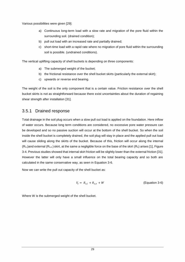
29
Various possibilities were given [29]:
a) Continuous long-term load with a slow rate and migration of the pore fluid within the
surrounding soil. (drained condition);
b) pull out load with an increased rate and partially drained;
c) short-time load with a rapid rate where no migration of pore fluid within the surrounding
soil is possible. (undrained conditions).
The vertical uplifting capacity of shell buckets is depending on three components:
a) The submerged weight of the bucket;
b) the frictional resistance over the shell bucket skirts (particularly the external skirt);
c) upwards or reverse end bearing.
The weight of the soil is the only component that is a certain value. Friction resistance over the shell
bucket skirts is not as straightforward because there exist uncertainties about the duration of regaining
shear strength after installation [31].
3.5.1 Drained response
Total drainage in the soil plug occurs when a slow pull out load is applied on the foundation. Here inflow
of water occurs. Because long term conditions are considered, no excessive pore water pressure can
be developed and so no passive suction will occur at the bottom of the shell bucket. So when the soil
inside the shell bucket is completely drained, the soil plug will stay in place and the applied pull out load
will cause sliding along the skirts of the bucket. Because of this, friction will occur along the internal
(Rs,i)and external (Rs,o ) skirt, at the same a negligible force on the base of the skirt (Re) arises [1], Figure
3-4. Previous studies showed that internal skirt friction will be slightly lower than the external friction [31].
However the latter will only have a small influence on the total bearing capacity and so both are
calculated in the same conservative way, as seen in Equation 3-6.
Now we can write the pull out capacity of the shell bucket as:
𝑉𝑠 = 𝑅𝑠,𝑖 + 𝑅𝑠,𝑜 + 𝑊 (Equation 3-6)
Where W is the submerged weight of the shell bucket.

30
3.5.2 Partially drained response
Even when an increasing applied pull out loading arises, a partial inflow of water takes place and so
passive suction occurs in the soil. This suction at the bottom of the shell foundation will be sufficient
enough to lift the soil plug together with the whole structure, Figure 3-5. So this uplift capacity will be
influenced by the weight of the soil plug (bottom resistance), the submerged weight of the shell bucket
and the friction between external skirt, as seen in Equation 3-7 [29].
𝑉𝑠 = 𝑅𝑏 + 𝑅𝑠,𝑜 + 𝑊 (Equation 3-7)
Figure 3-4: drained condition pull out
capacity [29]
Figure 3-5: Partially drained response [29]
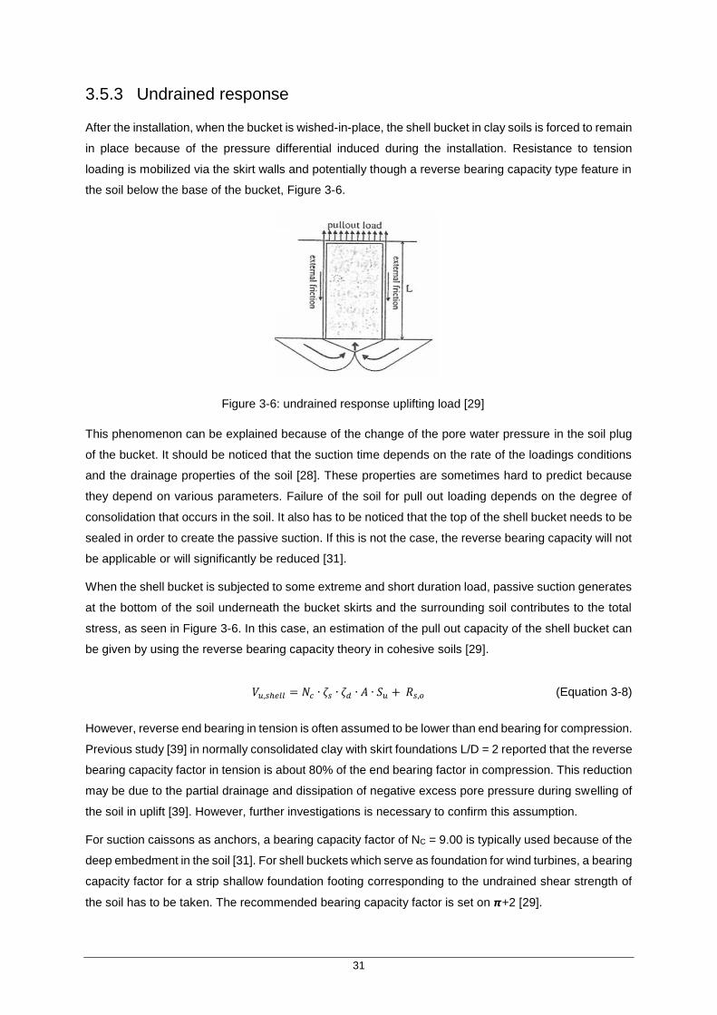
31
3.5.3 Undrained response
After the installation, when the bucket is wished-in-place, the shell bucket in clay soils is forced to remain
in place because of the pressure differential induced during the installation. Resistance to tension
loading is mobilized via the skirt walls and potentially though a reverse bearing capacity type feature in
the soil below the base of the bucket, Figure 3-6.
This phenomenon can be explained because of the change of the pore water pressure in the soil plug
of the bucket. It should be noticed that the suction time depends on the rate of the loadings conditions
and the drainage properties of the soil [28]. These properties are sometimes hard to predict because
they depend on various parameters. Failure of the soil for pull out loading depends on the degree of
consolidation that occurs in the soil. It also has to be noticed that the top of the shell bucket needs to be
sealed in order to create the passive suction. If this is not the case, the reverse bearing capacity will not
be applicable or will significantly be reduced [31].
When the shell bucket is subjected to some extreme and short duration load, passive suction generates
at the bottom of the soil underneath the bucket skirts and the surrounding soil contributes to the total
stress, as seen in Figure 3-6. In this case, an estimation of the pull out capacity of the shell bucket can
be given by using the reverse bearing capacity theory in cohesive soils [29].
𝑉𝑢,𝑠ℎ𝑒𝑙𝑙 = 𝑁𝑐 ∙ 𝜁𝑠 ∙ 𝜁𝑑 ∙ 𝐴 ∙ 𝑆𝑢 + 𝑅𝑠,𝑜 (Equation 3-8)
However, reverse end bearing in tension is often assumed to be lower than end bearing for compression.
Previous study [39] in normally consolidated clay with skirt foundations L/D = 2 reported that the reverse
bearing capacity factor in tension is about 80% of the end bearing factor in compression. This reduction
may be due to the partial drainage and dissipation of negative excess pore pressure during swelling of
the soil in uplift [39]. However, further investigations is necessary to confirm this assumption.
For suction caissons as anchors, a bearing capacity factor of NC = 9.00 is typically used because of the
deep embedment in the soil [31]. For shell buckets which serve as foundation for wind turbines, a bearing
capacity factor for a strip shallow foundation footing corresponding to the undrained shear strength of
the soil has to be taken. The recommended bearing capacity factor is set on 𝞹+2 [29].
Figure 3-6: undrained response uplifting load [29]
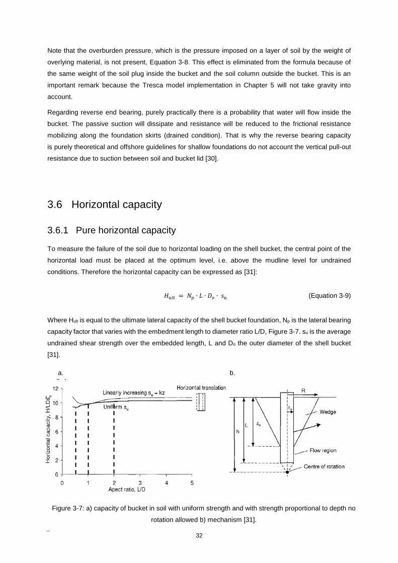
32
Note that the overburden pressure, which is the pressure imposed on a layer of soil by the weight of
overlying material, is not present, Equation 3-8. This effect is eliminated from the formula because of
the same weight of the soil plug inside the bucket and the soil column outside the bucket. This is an
important remark because the Tresca model implementation in Chapter 5 will not take gravity into
account.
Regarding reverse end bearing, purely practically there is a probability that water will flow inside the
bucket. The passive suction will dissipate and resistance will be reduced to the frictional resistance
mobilizing along the foundation skirts (drained condition). That is why the reverse bearing capacity
is purely theoretical and offshore guidelines for shallow foundations do not account the vertical pull-out
resistance due to suction between soil and bucket lid [30].
3.6 Horizontal capacity
3.6.1 Pure horizontal capacity
To measure the failure of the soil due to horizontal loading on the shell bucket, the central point of the
horizontal load must be placed at the optimum level, i.e. above the mudline level for undrained
conditions. Therefore the horizontal capacity can be expressed as [31]:
𝐻𝑢𝑙𝑡 = 𝑁𝑝 ∙ 𝐿 ∙ 𝐷𝑜 ∙ 𝑠𝑢 (Equation 3-9)
Where Hult is equal to the ultimate lateral capacity of the shell bucket foundation, Np is the lateral bearing
capacity factor that varies with the embedment length to diameter ratio L/D, Figure 3-7. su is the average
undrained shear strength over the embedded length, L and Do the outer diameter of the shell bucket
[31].
Figure 3-7: a) capacity of bucket in soil with uniform strength and with strength proportional to depth no
rotation allowed b) mechanism [31].
a. b.
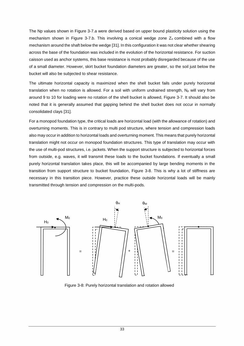
33
The Np values shown in Figure 3-7.a were derived based on upper bound plasticity solution using the
mechanism shown in Figure 3-7.b. This involving a conical wedge zone Zo combined with a flow
mechanism around the shaft below the wedge [31]. In this configuration it was not clear whether shearing
across the base of the foundation was included in the evolution of the horizontal resistance. For suction
caisson used as anchor systems, this base resistance is most probably disregarded because of the use
of a small diameter. However, skirt bucket foundation diameters are greater, so the soil just below the
bucket will also be subjected to shear resistance.
The ultimate horizontal capacity is maximized when the shell bucket fails under purely horizontal
translation when no rotation is allowed. For a soil with uniform undrained strength, Np will vary from
around 9 to 10 for loading were no rotation of the shell bucket is allowed, Figure 3-7. It should also be
noted that it is generally assumed that gapping behind the shell bucket does not occur in normally
consolidated clays [31].
For a monopod foundation type, the critical loads are horizontal load (with the allowance of rotation) and
overturning moments. This is in contrary to multi pod structure, where tension and compression loads
also may occur in addition to horizontal loads and overturning moment. This means that purely horizontal
translation might not occur on monopod foundation structures. This type of translation may occur with
the use of multi-pod structures, i.e. jackets. When the support structure is subjected to horizontal forces
from outside, e.g. waves, it will transmit these loads to the bucket foundations. If eventually a small
purely horizontal translation takes place, this will be accompanied by large bending moments in the
transition from support structure to bucket foundation, Figure 3-8. This is why a lot of stiffness are
necessary in this transition piece. However, practice these outside horizontal loads will be mainly
transmitted through tension and compression on the multi-pods.
M0 H0
Figure 3-8: Purely horizontal translation and rotation allowed
H0 M0
+ = =
θH θM

34
In the simplified model, the classic Vesic Equations determines if the structure is rigid or not, Appendix
A. If the shell bucket foundation is rigid, the angular rotations can be calculated as:
𝜃𝐻 = 6 ∙ 𝐻0
𝐿2∙𝑘 for the angular rotation due to H0 in the centerpoint on the top of the bucket
𝜃𝑀 = −12 ∙ 𝑀0
𝐿3∙𝑘 for the angular rotation due to M0 in the centerpoint on the top of the bucket
When purely horizontal translation occurs, the summation of the angular rotation due to H0 and M0 will
be zero, so M0 can be determined by:
<=> 𝜃𝐻 + 𝜃𝑀 = 0 (Equation 3-10)
<=> 6 ∙ 𝐻0
𝐿2∙𝑘 +
−12 ∙ 𝑀0
𝐿3∙𝑘 = 0
<=> 𝑀0 = 𝐻0∙𝐿
2 (Equation 3-11)
3.6.2 Allowance of rotation
When free rotation of the bucket is allowed, M0 is equal to zero and the normalized horizontal
capacity decreases to approximately 40% of the maximum horizontal capacity, Figure 3-9.
Figure 3-9: a) Capacity of bucket in soil with uniform strength and with strength proportional to depth and
rotation allowed b) mechanism [31]
a. b.
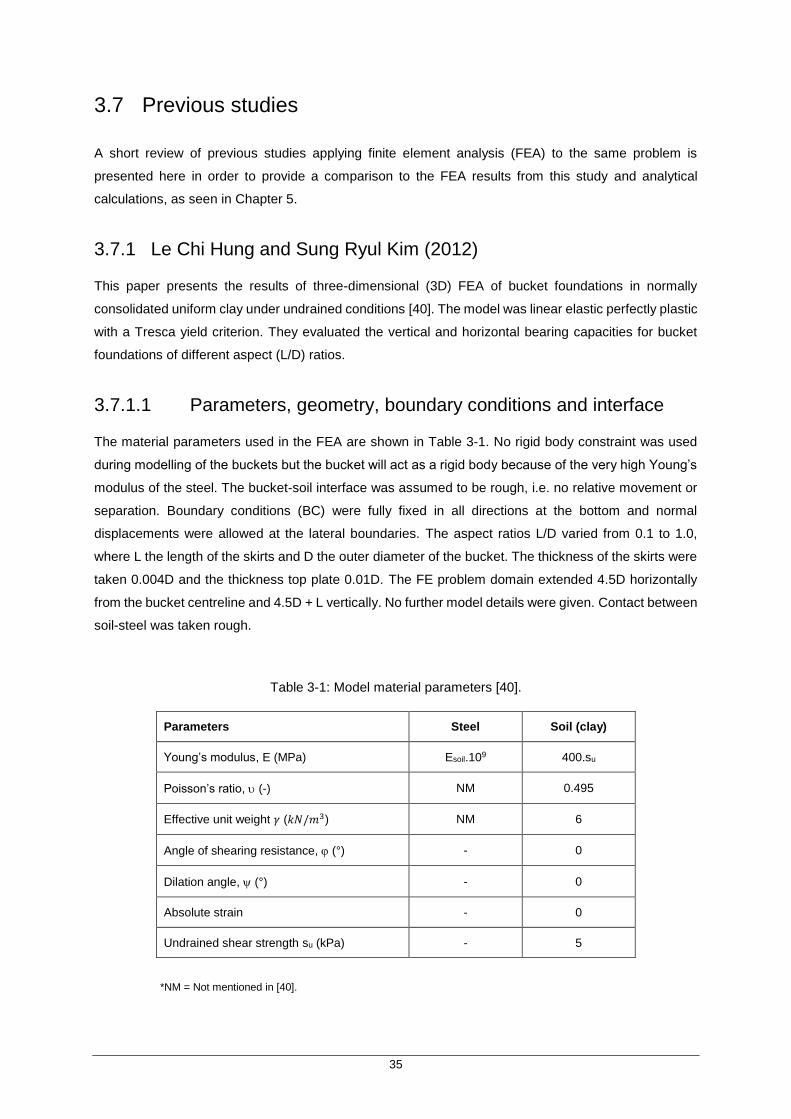
35
3.7 Previous studies
A short review of previous studies applying finite element analysis (FEA) to the same problem is
presented here in order to provide a comparison to the FEA results from this study and analytical
calculations, as seen in Chapter 5.
3.7.1 Le Chi Hung and Sung Ryul Kim (2012)
This paper presents the results of three-dimensional (3D) FEA of bucket foundations in normally
consolidated uniform clay under undrained conditions [40]. The model was linear elastic perfectly plastic
with a Tresca yield criterion. They evaluated the vertical and horizontal bearing capacities for bucket
foundations of different aspect (L/D) ratios.
3.7.1.1 Parameters, geometry, boundary conditions and interface
The material parameters used in the FEA are shown in Table 3-1. No rigid body constraint was used
during modelling of the buckets but the bucket will act as a rigid body because of the very high Young’s
modulus of the steel. The bucket-soil interface was assumed to be rough, i.e. no relative movement or
separation. Boundary conditions (BC) were fully fixed in all directions at the bottom and normal
displacements were allowed at the lateral boundaries. The aspect ratios L/D varied from 0.1 to 1.0,
where L the length of the skirts and D the outer diameter of the bucket. The thickness of the skirts were
taken 0.004D and the thickness top plate 0.01D. The FE problem domain extended 4.5D horizontally
from the bucket centreline and 4.5D + L vertically. No further model details were given. Contact between
soil-steel was taken rough.
Table 3-1: Model material parameters [40].
*NM = Not mentioned in [40].
Parameters Steel Soil (clay)
Young’s modulus, E (MPa) Esoil.109 400.su
Poisson’s ratio, (-) NM 0.495
Effective unit weight 𝛾 (𝑘𝑁/𝑚3) NM 6
Angle of shearing resistance, (°) - 0
Dilation angle, (°) - 0
Absolute strain - 0
Undrained shear strength su (kPa) - 5

36
3.7.1.2 Results
FE-results were given in terms of the normalized bearing capacities V / (A.su) and H / (A.su) in order to
compare gained results with other FEA’s. Vertical and horizontal displacements, respectively 𝑤 and 𝑢
were obtain from the reference point in the middle of the bucket lid. The normalized vertical load-
displacement curves according to different ratios are displayed in Figure 3-10 (a). The aspect ratios L/D
0.25, 0.5 and 1 respectively have an ultimate normalized vertical bearing capacity Vult / (A.su) of 8.7,
10.4 and 14, Figure 3-10.
Figure 3-11 (a, b) respectively shows the normalized horizontal load-displacement curves and the
ultimate horizontal capacity of the shell bucket foundation according to the L/D ratios where free rotation
was allowed. Here it can be said that Hult / (A.su) will increase linearly at L/D < 0.5 and the increasing
rate will decrease at L/D ≥ 0.5. Estimations of Hult / (A.su) according ratio L/D 0.5 and 1 are respectively
4.8 and 6.
`
Figure 3-11: Horizontal load-movement curve and capacity according to L/D ratios [40]
𝐻0
Figure 3-10: vertical load-movement curve and capacity according to L/D ratios [40]
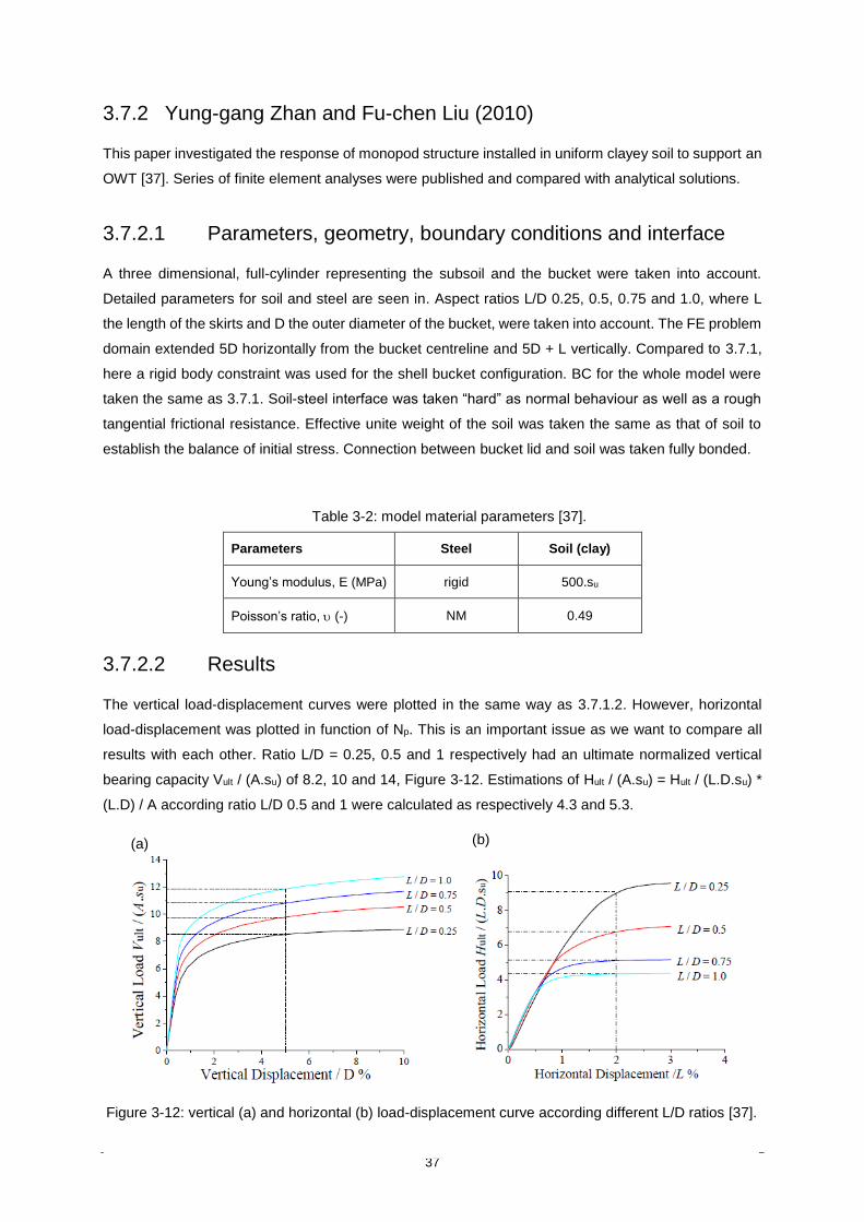
37
3.7.2 Yung-gang Zhan and Fu-chen Liu (2010)
This paper investigated the response of monopod structure installed in uniform clayey soil to support an
OWT [37]. Series of finite element analyses were published and compared with analytical solutions.
3.7.2.1 Parameters, geometry, boundary conditions and interface
A three dimensional, full-cylinder representing the subsoil and the bucket were taken into account.
Detailed parameters for soil and steel are seen in. Aspect ratios L/D 0.25, 0.5, 0.75 and 1.0, where L
the length of the skirts and D the outer diameter of the bucket, were taken into account. The FE problem
domain extended 5D horizontally from the bucket centreline and 5D + L vertically. Compared to 3.7.1,
here a rigid body constraint was used for the shell bucket configuration. BC for the whole model were
taken the same as 3.7.1. Soil-steel interface was taken “hard” as normal behaviour as well as a rough
tangential frictional resistance. Effective unite weight of the soil was taken the same as that of soil to
establish the balance of initial stress. Connection between bucket lid and soil was taken fully bonded.
Table 3-2: model material parameters [37].
3.7.2.2 Results
The vertical load-displacement curves were plotted in the same way as 3.7.1.2. However, horizontal
load-displacement was plotted in function of Np. This is an important issue as we want to compare all
results with each other. Ratio L/D = 0.25, 0.5 and 1 respectively had an ultimate normalized vertical
bearing capacity Vult / (A.su) of 8.2, 10 and 14, Figure 3-12. Estimations of Hult / (A.su) = Hult / (L.D.su) *
(L.D) / A according ratio L/D 0.5 and 1 were calculated as respectively 4.3 and 5.3.
Parameters Steel Soil (clay)
Young’s modulus, E (MPa) rigid 500.su
Poisson’s ratio, (-) NM 0.49
(a) (b)
Figure 3-12: vertical (a) and horizontal (b) load-displacement curve according different L/D ratios [37].

38
3.7.3 H.A. Taiebat and J.P. Carter (2005)
The paper presents the results of series of numerical analyses of caisson foundations under undrained
conditions where the aspect ratios L/D were taken higher than 1. It was also assumed that the soil obeys
the Tresca failure criterion [41].
3.7.3.1 Parameters, geometry, Boundary conditions and interface
A three dimensional, half-cylinder representing the subsoil and the bucket was taken into account.
Aspect ratios L/D 2 and 4, where L the length of the skirts and D the outer diameter of the bucket, were
taken into account. The FE problem domain extended 4D horizontally from the bucket centreline and
3.5 L vertically. BC for the whole model were taken the same as 3.7.1. Connection between bucket lid
and soil was taken fully bonded. Young’s modulus was taken Eu = 300su and the bucket was made rigid
by the use of E = 1000 Eu .No further important info was given.
3.7.3.2 Results
The normalized axial resistance of the caisson predicted by the FEA at vertical displacement of 5% of
the caisson diameter is Vult / (A.su) = 15 for ratio L/D = 2 and 23 for L/D = 4, Figure 3-13. Estimations of
Hult / (A.su) according ratio L/D 2 and 4 were calculated as respectively 9.7 and 20.
Figure 3-13: vertical (a) and horizontal (b) load-displacement curve according different L/D ratios [41].

39
Chapter 4
Linear Elastic FEA
4 Linear Elatic FEA
In the beginning of this chapter, two- and three-dimensional solid bucket foundations are modelled using
elastic theory. These models are less complex in geometry than shell bucket foundations and more
obvious to carry out numerical analysis with the finite element analysis ABAQUS/CAE. The numerical
analyses for the settlement of the elastic solid bucket models are subsequently compared with analytical
calculations based on [25]. Finally, elastic analysis of shell buckets is presented however in this case
there are no analytical solutions with which a comparison can be made.
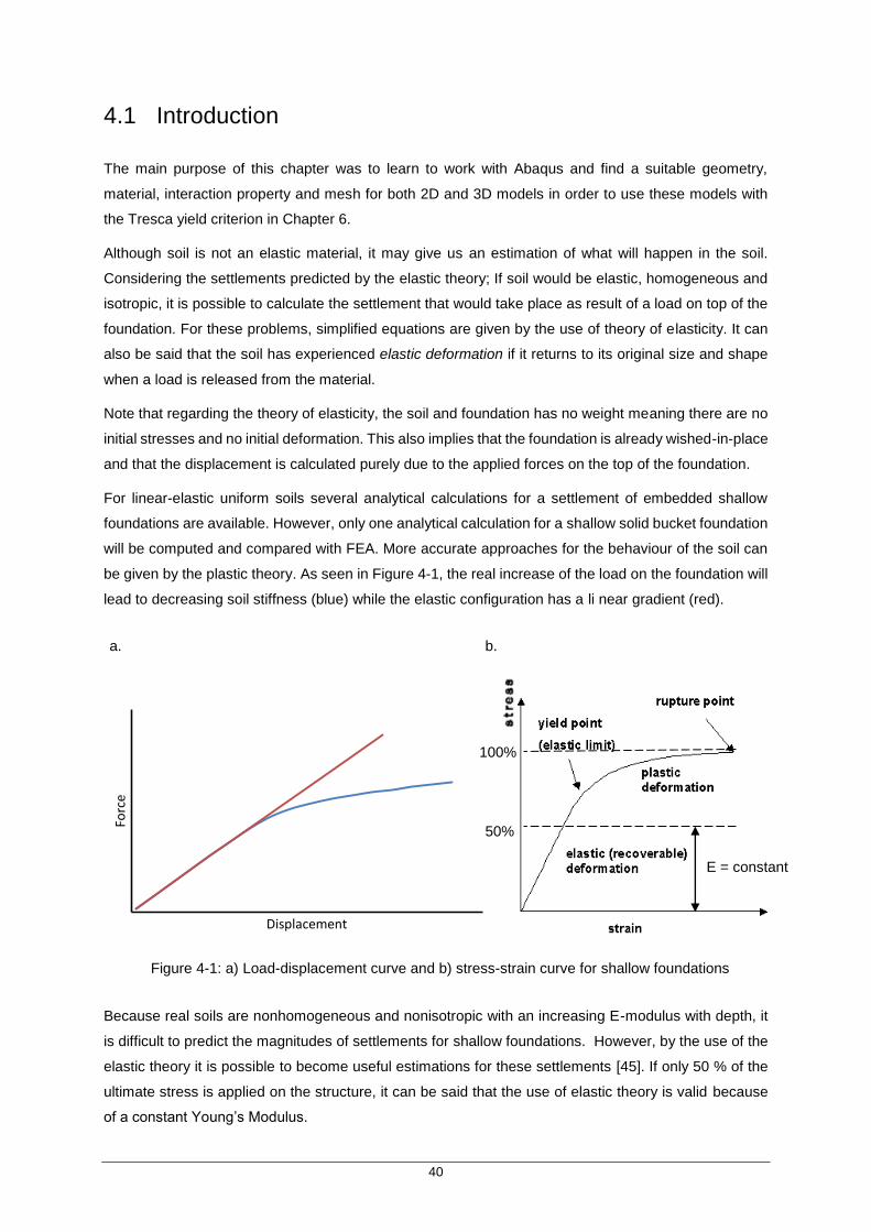
40
4.1 Introduction
The main purpose of this chapter was to learn to work with Abaqus and find a suitable geometry,
material, interaction property and mesh for both 2D and 3D models in order to use these models with
the Tresca yield criterion in Chapter 6.
Although soil is not an elastic material, it may give us an estimation of what will happen in the soil.
Considering the settlements predicted by the elastic theory; If soil would be elastic, homogeneous and
isotropic, it is possible to calculate the settlement that would take place as result of a load on top of the
foundation. For these problems, simplified equations are given by the use of theory of elasticity. It can
also be said that the soil has experienced elastic deformation if it returns to its original size and shape
when a load is released from the material.
Note that regarding the theory of elasticity, the soil and foundation has no weight meaning there are no
initial stresses and no initial deformation. This also implies that the foundation is already wished-in-place
and that the displacement is calculated purely due to the applied forces on the top of the foundation.
For linear-elastic uniform soils several analytical calculations for a settlement of embedded shallow
foundations are available. However, only one analytical calculation for a shallow solid bucket foundation
will be computed and compared with FEA. More accurate approaches for the behaviour of the soil can
be given by the plastic theory. As seen in Figure 4-1, the real increase of the load on the foundation will
lead to decreasing soil stiffness (blue) while the elastic configuration has a li near gradient (red).
Because real soils are nonhomogeneous and nonisotropic with an increasing E-modulus with depth, it
is difficult to predict the magnitudes of settlements for shallow foundations. However, by the use of the
elastic theory it is possible to become useful estimations for these settlements [45]. If only 50 % of the
ultimate stress is applied on the structure, it can be said that the use of elastic theory is valid because
of a constant Young’s Modulus.
a. b.
Forc
e
Displacement
Figure 4-1: a) Load-displacement curve and b) stress-strain curve for shallow foundations
100%
50%
E = constant
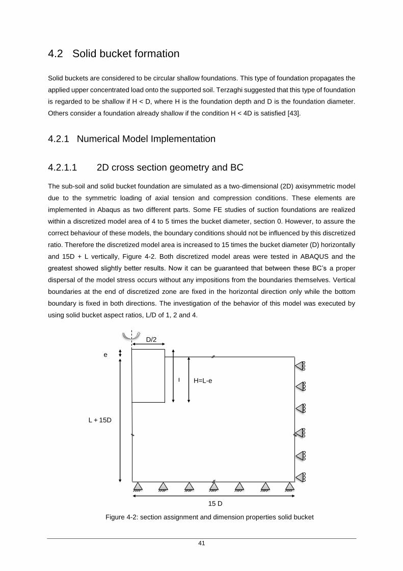
41
4.2 Solid bucket formation
Solid buckets are considered to be circular shallow foundations. This type of foundation propagates the
applied upper concentrated load onto the supported soil. Terzaghi suggested that this type of foundation
is regarded to be shallow if H < D, where H is the foundation depth and D is the foundation diameter.
Others consider a foundation already shallow if the condition H < 4D is satisfied [43].
4.2.1 Numerical Model Implementation
4.2.1.1 2D cross section geometry and BC
The sub-soil and solid bucket foundation are simulated as a two-dimensional (2D) axisymmetric model
due to the symmetric loading of axial tension and compression conditions. These elements are
implemented in Abaqus as two different parts. Some FE studies of suction foundations are realized
within a discretized model area of 4 to 5 times the bucket diameter, section 0. However, to assure the
correct behaviour of these models, the boundary conditions should not be influenced by this discretized
ratio. Therefore the discretized model area is increased to 15 times the bucket diameter (D) horizontally
and 15D + L vertically, Figure 4-2. Both discretized model areas were tested in ABAQUS and the
greatest showed slightly better results. Now it can be guaranteed that between these BC’s a proper
dispersal of the model stress occurs without any impositions from the boundaries themselves. Vertical
boundaries at the end of discretized zone are fixed in the horizontal direction only while the bottom
boundary is fixed in both directions. The investigation of the behavior of this model was executed by
using solid bucket aspect ratios, L/D of 1, 2 and 4.
e
D/2
L
L + 15D
15 D
H=L-e
Figure 4-2: section assignment and dimension properties solid bucket

42
Where
D = Solid Bucket diameter = 8 m
L = Length of the solid bucket varying from ratio
e = Protrusion of the solid bucket above the seabed = 0.15 m
H = L- e = Bucket embedment depth varying from ratio
4.2.1.2 Parameters
The solid bucket foundation is assumed to be linear elastic with a Young’s modulus of 210 GPa and a
Poisson´s ratio of 0.2. The elastic response of the soil is assumed to be linear, homogenous and
isotropic with a constant Young’s modulus of 40MPa and a Poisson ratio of 0.495. The density for steel
and soil are 7850 kg/m3 and 2000 kg/m3 respectively.
4.2.1.3 Interaction properties
A surface to surface type interface was implemented to provide frictional contact between the base of
the solid bucket and soil part (pink dashed line). A rough contact with no separation allowed was used.
In order to correspond to elastic analytical calculations for the settlement of a shallow foundation, the
interface between the side of the bucket and the soil was assumed to be frictionless, Figure 4-3.
Slip will occur because of the
frictionless tangential behavior.
Loads on the top of the solid
bucket are converted into
pressures applied to the
supporting soil by the use of
normal “hard” contact
behavior.
Figure 4-3: interaction properties solid bucket elastic model
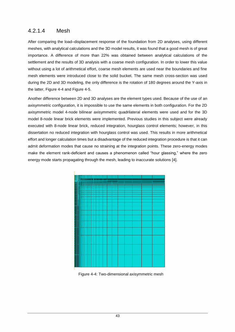
43
4.2.1.4 Mesh
After comparing the load–displacement response of the foundation from 2D analyses, using different
meshes, with analytical calculations and the 3D model results, it was found that a good mesh is of great
importance. A difference of more than 22% was obtained between analytical calculations of the
settlement and the results of 3D analysis with a coarse mesh configuration. In order to lower this value
without using a lot of arithmetical effort, coarse mesh elements are used near the boundaries and fine
mesh elements were introduced close to the solid bucket. The same mesh cross-section was used
during the 2D and 3D modeling, the only difference is the rotation of 180 degrees around the Y-axis in
the latter, Figure 4-4 and Figure 4-5.
Another difference between 2D and 3D analyses are the element types used. Because of the use of an
axisymmetric configuration, it is impossible to use the same elements in both configuration. For the 2D
axisymmetric model 4-node bilinear axisymmetric quadrilateral elements were used and for the 3D
model 8-node linear brick elements were implemented. Previous studies in this subject were already
executed with 8-node linear brick, reduced integration, hourglass control elements; however, in this
dissertation no reduced integration with hourglass control was used. This results in more arithmetical
effort and longer calculation times but a disadvantage of the reduced integration procedure is that it can
admit deformation modes that cause no straining at the integration points. These zero-energy modes
make the element rank-deficient and causes a phenomenon called “hour glassing,” where the zero
energy mode starts propagating through the mesh, leading to inaccurate solutions [4].
Figure 4-4: Two-dimensional axisymmetric mesh

44
4.2.2 Immediate settlement of the solid bucket
4.2.2.1 Analytical calculation
Analytical calculation of the immediate settlement for solid bucket configuration was carry out using
Equation 2-1. Detailed calculation for L/D = 1 can be found in appendix B. First calculations are executed
with a concentrated load of 100 kN that can be converted to a net foundation pressure of 1989 kPa. To
compare different analytical results with numerical 2D and 3D FEA, concentrated loads of 400kN and
850 kN were also considered. The largest force is an estimated vertical force for a 3.0 MW Turbine of
90 meter hub height where the vertical reaction force is divided on three separate solid bucket
foundations.
Table 1: Analytical calculation of shallow foundation settlements
L/D ratio Settlement, Si (mm) for each load case
100 kN 400 kN 850 kN
1 - 0.17 - 0.68 - 1.45
2 - 0.15 - 0.60 - 1.27
4 - 0.14 - 0.54 - 1.15
Figure 4-5 : Three-dimensional axisymmetric mesh

45
4.2.2.2 Comparison analytical with numerical FE results.
A main trend regarding 2D and 3D numerical results is the stabilization of the relative settlement after
applying more load, see graph in Figure 4-6. The relative settlement (RS) in vertical direction can be
calculated with Equation 4.1
𝑅𝑆 (%) = |(𝐴𝑆−𝐴𝑁𝑆)
𝐴𝑆| 𝑥 100 (Equation 4-1)
Where
AS = Analytical settlement
ANS = Average numerical settlement in each node of the top bucket surface
As seen in Table 4-1, the RS for 2D and 3D solid bucket configuration L/D = 1 vary from 7% to 8%. If
both 2D and 3D settlement results are compared with each other, only a difference of 1 % occurs. The
same calculations can be done for the ratios L/D = 2 and 4. Here the RS for 2D and 3D solid bucket
configuration L/D = 2 vary from 12 % to 17 % and for L/D = 4 around 20 %. Differences between 2D and
3D ANS for L/D = 2 and 4 are both about 4%.
The high RS (%) for L/D = 4 can be explained due to inaccurate approximations of the influence factor
(If) or depth factor (cd). If, for example, the analytical calculation was done with a slightly higher If , i.e.
for flexible instead of rigid foundation, the RS would be around 10 %. Another explanation for this
difference is that the analytical calculation may not be suitable for large L/D ratios.
6,7
6,75
6,8
6,85
6,9
0 200 400 600 800 1000
Rel
ativ
ely
sett
lem
ent
(%
)
Load (kN)
3D Aspect ratio L/D = 1
7,4
7,45
7,5
7,55
7,6
7,65
0 200 400 600 800 1000
Rel
ativ
ely
sett
lem
ent
(%)
Load (kN)
2D Aspect ratio L/D = 1
Figure 4-6: Comparison of analytical and 2D (left) and 3D (right) numerical settlement ratio L/D = 1

46
Table 4-1: Solid Bucket Aspect ratio L/D = 1 evaluation method settlements comparison (mm)
4.3 Shell bucket
Compared to the solid bucket, the shell bucket foundation has soil inside a thin outer skirt structure. It
can effectively be described as an upturned bucket that is embedded in the soil. In practical, due to
irregularities in the sea floor, a small gap may be left between bucket lid and seafloor. This was also
taken into account during modelling. Here, only 2D and 3D analyses for a shell bucket with an aspect
ratio of 1, 2 and 4 will be compared because no analytical elastic solutions are available for comparison.
4.3.1 Numerical Model Implementation
4.3.1.1 2D cross section geometry and boundaries conditions
A simplified model was designed in order to compare 2D and 3D numerical calculations. Due to the
symmetric loading condition only a 2D axis-symmetric model was used to represent the sub-soil and
suction caisson or shell bucket, Figure 4-7. The discretized model was taken the same as the solid
bucket configuration so the area had a dimension of 15 times the bucket diameter (D) in horizontal
alignment and 15 D + L in vertical alignment. Within these boundaries, the calculated behavior of the
shell bucket is not significantly influenced.
EVALUATION METHOD
100KN 400KN 850KN
AS - 0.17 - 0.68 - 1.45
ANS2D -0.18 -0.74 -1.56
ANS3D -0.18 -0.73 -1.55
RSANALYTICAL_2D (%) 7.51 7.60 7.62
RSANALYTICAL_3D (%) 6.81 6.85 6.85
COMPARISSON 2D AND 3D (%)
0.65 0.70 0.71

47
Geometric parameters for L/D = 1:
D = 8m
L = 8m
e = 0.15 m (Space between seabed and upper skirt of shell bucket)
t = 0.02 m (Bucket wall thickness)
f = 0.03 m (Bucket lid thickness)
4.3.1.2 Parameters
Exactly the same parameters were used for the shell bucket configuration as for the solid bucket
configuration, as seen in 4.2.1.2. The only difference between both is the geometry of the bucket itself
and the use of a rigid body constraint in the shell bucket assembly. The advantages of this latter setting
is that relative positions of the regions that are part of the rigid body remain constant throughout the
analysis. This means that the shell bucket will transmit the loads but will not deform. If no rigid body is
used, the shell bucket would deform under loads. If this assumption was not done, it would be needed
to model the shell bucket including stiffening elements near the lid and along the bucket skirts. Problems
may occur in due to the steel failure so a simplified model was needed.
D/2
L
t
L + 15 D
15 D
f
e
Figure 4-7: section assignment and dimension properties shell bucket

48
4.3.1.3 Interaction properties
Where the solid buckets had no tangential behavior in order to correspond to analytical calculations, the
tangential behavior in the shell bucket is assumed to be rough and no separation of the contacts was
allowed. In effect, the nodes of the shell bucket sides and nodes on the soil sides are “stuck” together
so the occurrence of slip is not allowed, Figure 4-8 (blue dashed line). It can be seen that with these
properties, downwards movement of the bucket develops upwards skirt friction between the skirt and
the surrounding soil.
4.3.1.4 Mesh
In both, solid and shell analyses, almost same meshing geometry was used. In the 2D analyses, element
types were the same as the solid bucket configuration.
In the elastic 3D-model the part soil consists of two different element types in order to avoid poor element
shapes in our mesh. As seen in Figure 4-9 (a), the elements indicated in green underneath the shell
bucket, which is colored red, were 6-node linear triangular prisms and the soil material elements outside
the bucket were 8-node linear bricks. In Figure 4-9 (b) where the shell bucket is removed for clarity, the
difference in shape between both elements can be seen.
Note that these element type settings will be changed in Chapter 5 in order to give more accurate results.
Figure 4-8: interaction properties shell bucket
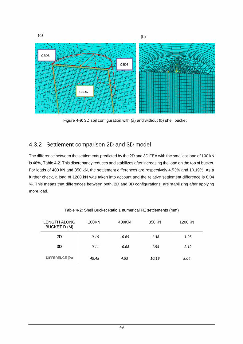
49
4.3.2 Settlement comparison 2D and 3D model
The difference between the settlements predicted by the 2D and 3D FEA with the smallest load of 100 kN
is 48%, Table 4-2. This discrepancy reduces and stabilizes after increasing the load on the top of bucket.
For loads of 400 kN and 850 kN, the settlement differences are respectively 4.53% and 10.19%. As a
further check, a load of 1200 kN was taken into account and the relative settlement difference is 8.04
%. This means that differences between both, 2D and 3D configurations, are stabilizing after applying
more load.
Table 4-2: Shell Bucket Ratio 1 numerical FE settlements (mm)
LENGTH ALONG BUCKET D (M)
100KN 400KN 850KN 1200KN
2D - 0.16 - 0.65 -1.38 - 1.95
3D - 0.11 - 0.68 -1.54 - 2.12
DIFFERENCE (%) 48.48 4.53 10.19 8.04
C3D8
C3D8
C3D6
(a) (b)
Figure 4-9: 3D soil configuration with (a) and without (b) shell bucket
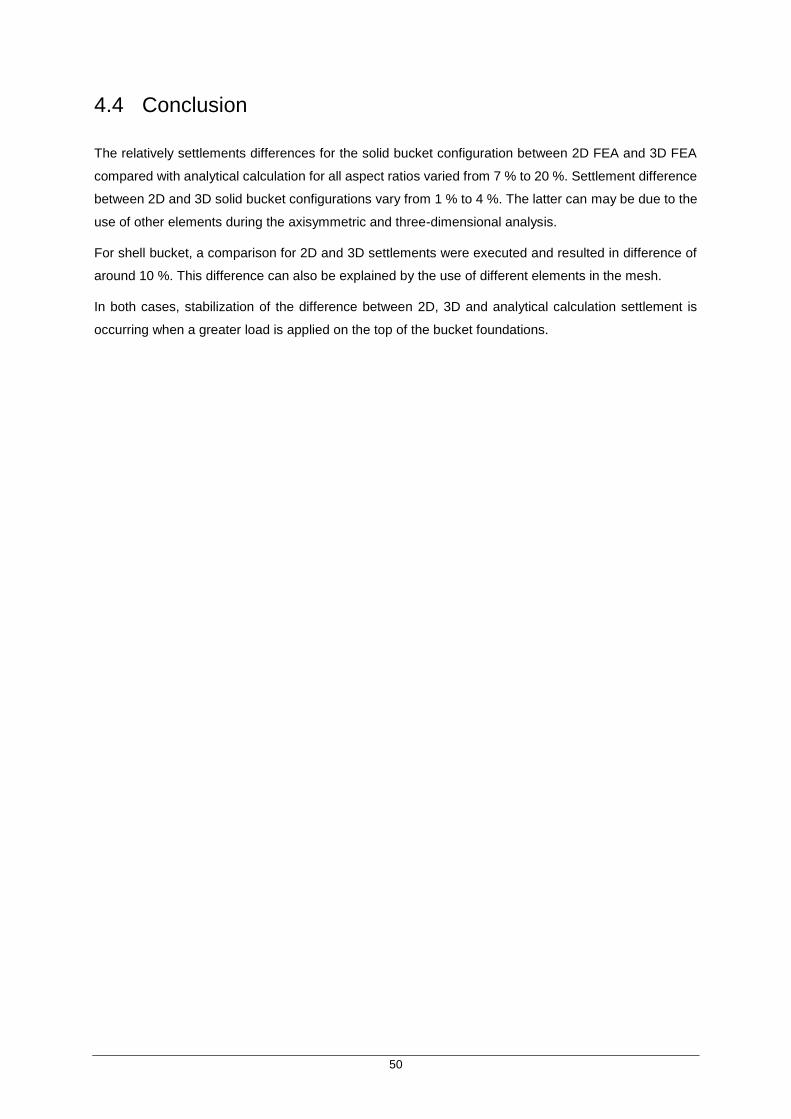
50
4.4 Conclusion
The relatively settlements differences for the solid bucket configuration between 2D FEA and 3D FEA
compared with analytical calculation for all aspect ratios varied from 7 % to 20 %. Settlement difference
between 2D and 3D solid bucket configurations vary from 1 % to 4 %. The latter can may be due to the
use of other elements during the axisymmetric and three-dimensional analysis.
For shell bucket, a comparison for 2D and 3D settlements were executed and resulted in difference of
around 10 %. This difference can also be explained by the use of different elements in the mesh.
In both cases, stabilization of the difference between 2D, 3D and analytical calculation settlement is
occurring when a greater load is applied on the top of the bucket foundations.

51
Chapter 5
Elasto-Plastic FEA
5 Elasto-Plastic FEA
In this dissertation only short term stability problems of saturated clays will be discussed. This means
that the undrained condition can reasonably be assumed to carry out total stress analysis. Therefore,
the soil is modelled as a linear elastic perfectly plastic material with a Tresca failure criterion [46].
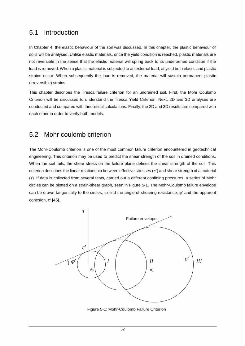
52
5.1 Introduction
In Chapter 4, the elastic behaviour of the soil was discussed. In this chapter, the plastic behaviour of
soils will be analysed. Unlike elastic materials, once the yield condition is reached, plastic materials are
not reversible in the sense that the elastic material will spring back to its undeformed condition if the
load is removed. When a plastic material is subjected to an external load, at yield both elastic and plastic
strains occur. When subsequently the load is removed, the material will sustain permanent plastic
(irreversible) strains.
This chapter describes the Tresca failure criterion for an undrained soil. First, the Mohr Coulomb
Criterion will be discussed to understand the Tresca Yield Criterion. Next, 2D and 3D analyses are
conducted and compared with theoretical calculations. Finally, the 2D and 3D results are compared with
each other in order to verify both models.
5.2 Mohr coulomb criterion
The Mohr-Coulomb criterion is one of the most common failure criterion encountered in geotechnical
engineering. This criterion may be used to predict the shear strength of the soil in drained conditions.
When the soil fails, the shear stress on the failure plane defines the shear strength of the soil. This
criterion describes the linear relationship between effective stresses (𝜎’) and shear strength of a material
(𝜏). If data is collected from several tests, carried out a different confining pressures, a series of Mohr
circles can be plotted on a strain-shear graph, seen in Figure 5-1. The Mohr-Coulomb failure envelope
can be drawn tangentially to the circles, to find the angle of shearing resistance, ' and the apparent
cohesion, c' [45].
𝜏
𝜏
===
===
𝐼
𝐼
𝜎′
𝜎
𝜑’
𝜎3
𝜎
𝜎1
𝜎
Failure envelope
𝐼𝐼𝐼
𝐼𝐼𝐼
𝐼𝐼
𝐼𝐼
𝑐′
𝑐′
Figure 5-1: Mohr-Coulomb Failure Criterion

53
This relation can be expressed as the following Equation 5-1:
𝜏𝑚𝑎𝑥 ≤ 𝜎′ ∙ tan 𝜑′ + 𝑐′ (Equation 5-1)
Where
c’ = the apparent cohesion of the soil (intercept of the failure envelope with the axis);
' = the angle of shearing resistance (slope of the failure envelope);
𝜎’ = 𝜎 – u = total stress – pore water pressure = the normal effective stress;
𝜏max = the maximum shear stress.
If the shear stress (𝜏) that is caused by a load remains smaller than the shear strength of the soil defined
by the Mohr-Coulomb criteria, then only elastic deformation will occur in the soil. Note that it is not
possible to have a stress state out outside the criteron, failure occurs when shear stress is on the failure
envelope. It also has to be noticed that some models use hardening rule that allows the yield surface to
expand. As a perfectly plastic model is assumed, this will not be taken into account.
5.3 Tresca Yield criterion
For the interpretation of the shear strength of a clay soil in undrained conditions and constant volume
shearing, the Tresca theory by Henri Tresca can be used [45]. Undrained response is described in terms
of total stress and the pore water pressure is not known. The shear strength under undrained conditions
is called undrained shear strength su. This criterion can be seen as a reduced Mohr-coulomb criterion
where the angle of internal friction 𝜑 = 0. As seen in Figure 5-2, the undrained shear strength 𝑠𝑢 is the
radius of Mohr circle with 𝜎1 the major principal stress and 𝜎3 is the minor principal stress which gives
the Equation 5-2:
𝑠𝑢 = (𝜎1−𝜎3)
2 (Equation 5-2)
Note that the shear strength under undrained loading only depends on the void ratio or initial water
content or initial total confining pressure. This assumption regarding the soil response is used where the
loading rate is much greater than the rate at which pore water pressures can dissipate, e.g. dynamic
environmental loads on offshore structures.

54
5.4 Two-dimensional analysis
2D models were developed for the analysis of solid and shell bucket configurations. Below, the
implementation of the numerical model is discussed and model validation is conducted. Subsequently,
the theoretical load-displacement calculations for both configurations are evaluated and compared to
the load-displacement predicted by the FEA.
5.4.1 Numerical model implementation
The elastic two dimensional model used in Figure 4-7, was adopted but was subject to some changes
as follows:
a) the soil material parameters were changed in order to define them as an elastic-perfectly plastic
material according the Tresca yield criterion;
b) the overall mesh was taken finer in order to avoid extensive distortion of the elements;
c) an extra boundary condition was set on the rigid body part to prevent the bucket against
unwanted movements.
d) Shell buckets in in the elastic models were assumed to have a gap between bucket lid and
seafloor. In this Chapter a configuration with and without a gap was modelled.
These changes add some degree of complexity to the program which resulted in longer run times.
However, compared to the 3D models, the 2D analyses are fast. The changes and the overall
characteristics of the foundation model are discussed in the following sections.
𝜏
𝜏
𝜎
𝜎
𝜎3
𝜎
𝜎1
𝜎
𝑐′ = 𝑠𝑢
Type equation here.
Figure 5-2: Tresca yield criterion
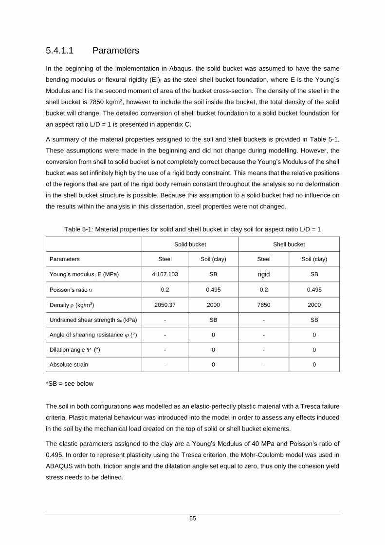
55
5.4.1.1 Parameters
In the beginning of the implementation in Abaqus, the solid bucket was assumed to have the same
bending modulus or flexural rigidity (EI)f as the steel shell bucket foundation, where E is the Young´s
Modulus and I is the second moment of area of the bucket cross-section. The density of the steel in the
shell bucket is 7850 kg/m3, however to include the soil inside the bucket, the total density of the solid
bucket will change. The detailed conversion of shell bucket foundation to a solid bucket foundation for
an aspect ratio L/D = 1 is presented in appendix C.
A summary of the material properties assigned to the soil and shell buckets is provided in Table 5-1.
These assumptions were made in the beginning and did not change during modelling. However, the
conversion from shell to solid bucket is not completely correct because the Young’s Modulus of the shell
bucket was set infinitely high by the use of a rigid body constraint. This means that the relative positions
of the regions that are part of the rigid body remain constant throughout the analysis so no deformation
in the shell bucket structure is possible. Because this assumption to a solid bucket had no influence on
the results within the analysis in this dissertation, steel properties were not changed.
Table 5-1: Material properties for solid and shell bucket in clay soil for aspect ratio L/D = 1
Solid bucket Shell bucket
Parameters Steel Soil (clay) Steel Soil (clay)
Young’s modulus, E (MPa) 4.167.103 SB rigid SB
Poisson’s ratio 0.2 0.495 0.2 0.495
Density (kg/m3) 2050.37 2000 7850 2000
Undrained shear strength su (kPa) - SB - SB
Angle of shearing resistance φ (°) - 0 - 0
Dilation angle 𝛹 (°) - 0 - 0
Absolute strain - 0 - 0
*SB = see below
The soil in both configurations was modelled as an elastic-perfectly plastic material with a Tresca failure
criteria. Plastic material behaviour was introduced into the model in order to assess any effects induced
in the soil by the mechanical load created on the top of solid or shell bucket elements.
The elastic parameters assigned to the clay are a Young’s Modulus of 40 MPa and Poisson’s ratio of
0.495. In order to represent plasticity using the Tresca criterion, the Mohr-Coulomb model was used in
ABAQUS with both, friction angle and the dilatation angle set equal to zero, thus only the cohesion yield
stress needs to be defined.
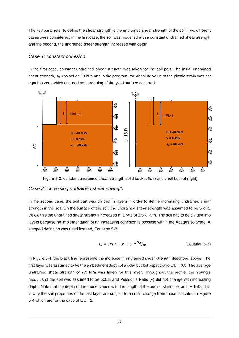
56
The key parameter to define the shear strength is the undrained shear strength of the soil. Two different
cases were considered; in the first case, the soil was modelled with a constant undrained shear strength
and the second, the undrained shear strength increased with depth.
Case 1: constant cohesion
In the first case, constant undrained shear strength was taken for the soil part. The initial undrained
shear strength, su was set as 60 kPa and in the program, the absolute value of the plastic strain was set
equal to zero which ensured no hardening of the yield surface occurred.
Case 2: increasing undrained shear strength
In the second case, the soil part was divided in layers in order to define increasing undrained shear
strength in the soil. On the surface of the soil, the undrained shear strength was assumed to be 5 kPa.
Below this the undrained shear strength increased at a rate of 1.5 kPa/m. The soil had to be divided into
layers because no implementation of an increasing cohesion is possible within the Abaqus software. A
stepped definition was used instead, Equation 5-3.
𝑠𝑢 = 5𝑘𝑃𝑎 + 𝑥 ∙ 1.5 𝑘𝑃𝑎𝑚⁄ (Equation 5-3)
In Figure 5-4, the black line represents the increase in undrained shear strength described above. The
first layer was assumed to be the embedment depth of a solid bucket aspect ratio L/D = 0.5. The average
undrained shear strength of 7.9 kPa was taken for this layer. Throughout the profile, the Young’s
modulus of the soil was assumed to be 500su and Poisson’s Ratio () did not change with increasing
depth. Note that the depth of the model varies with the length of the bucket skirts, i.e. as L + 15D. This
is why the soil properties of the last layer are subject to a small change from those indicated in Figure
5-4 which are for the case of L/D =1.
L H=L-e
15D
E = 40 MPa
ν = 0.495
su = 60 kPa
L
L +
15 D
E = 40 MPa
ν = 0.495
su = 60 kPa
H=L-e
Figure 5-3: constant undrained shear strength solid bucket (left) and shell bucket (right)

57
5.4.1.2 Geometry, boundary conditions, interaction properties and
mesh
As already mentioned in section 5.4.1, the elastic model Figure 4-7 was adopted but subject to some
changes. Geometry and boundary conditions were taken the same as those used for the elastic model.
Figure 5-4: Undrained shear strength depending on the soil depth for L/D =1 (not to scale).

58
The slight changes that were done:
To avoid elements with aspect ratios that would lead to numerical instability, the mesh had to
remain fine all the way to the outer boundary of the mesh. This meant that there were many
more elements within the mesh and lead to longer run time in the analyses;
To ensure the pile displaced in the vertical direction only, horizontal displacements of the bucket
lid were set to zero. Because of the use of the axisymmetric model, the bucket should not move
in the horizontal direction however some small horizontal displacement was seen in the initial
FEA results and so the above restraint was applied in subsequent analyses. This boundary
condition also happened to improve the calculation time of the models.
For the soil-bucket interface, the interaction properties were also set the same as the elastic
configuration. This means a perfectly rough interface was considered between bucket and soil.
However, by the use of the Tresca Model, the interface assumption that was used still allows the soil
elements next to the bucket to mobilize the full undrained shearing resistance of the soil.
To understand the reverse bearing capacity theory that will discussed in section 3.5, shell buckets with
ratio L/D = 0.5, 1 and 2 without a gap configuration are also executed. Here a fully bonded interface
between the bucket lid and seafloor was assumed with a “tied” constraint.
5.4.2 Shear analysis and results
Shear strength describes the magnitude of shear stress that a soil can sustain. The undrained shear
strength is already defined in Tresca yield criterion. Note that the no elastic volumetric strains occur, the
Poisson’s ratio stays constant and no self-weight of was assumed. These assumptions are of great
importance in order to do the FEA.
5.4.2.1 Model Validation
To check if the assembled models are correct, the FEA was compared to an analytical evaluation of the
vertical installation bearing capacity. The displacement-load analysis was carried out with the shell
bucket ratio L/D = 1 – Case 1. To ensure the soil next to the bucket skirt is mobilized, the arbitrary
displacement of the shell bucket was taken s = -0.12 m. The bearing capacity factor for shallow
foundations was set to Nc = 5.14. Detailed calculations can be found in appendix D.
This resulted in a numerical vertical bearing load of Vs=-0.12,R_1,numerical = 26145 kN, Figure 5-5.

59
It can be said that the difference between the numerical results and analytical calculation is
approximately 7% which is acceptable because the bearing capacity factor is an estimated factor.
Within this dissertation a space between the mudline and the shell bucket of 15 cm was assumed;
however, this gap will disappear when the vertical load is increasing or when suction is applied in this
zone. Due to the under pressure in the gap, the bucket will penetrate itself into the clay soil. When the
gap is closed, the vertical bearing capacity will increase because of the compression of the soil
underneath the lid of the bucket. The ultimate vertical bearing capacity is discussed in Section 5.4.3
where more detailed equations are used. These calculations can be compared with the installation of
the shell bucket.
5.4.2.2 Solid bucket
With the solid bucket configuration, the outer side and base of the bucket will be subjected to shear. In
In Case 1, when an undrained shear strength of 60 kPa is assumed in the whole model, the shear stress
along the sides of the solid bucket reached the undrained shear stress su after a displacement of 0.08
m for L/D = 0.5 and 0.06 m for L/D = 2, Figure 5-6. It can be said that all solid bucket configurations with
a displacement > 0.08 m are fully mobilized along the outer bucket wall.
In Case 2, where the undrained shear strength increases with depth, the bucket with aspect ratio L/D =
0.5 is mobilized along the outer sides after a displacement of 0.10 m, Figure 5-7. It can also be seen
that the embedment of the bucket only occurs in one uniform layer with su = 7.9 kPa. For a bucket
configuration with aspect ratio L/D = 2, there is an increase of the undrained shear strength at depths of
4 m and 8 m. Because of the transition from one layer to another with higher undrained shear strength,
the mobilized undrained shear strength goes suddenly from 7.9 kPa to 13.8 kPa and eventually to 22.8
kPa, as seen in Figure 5-7. The solid bucket is mobilized after a displacement of 0.04 m. These values
are representative regarding Figure 5-4.
Displacement (m)
Load (kN)
0.00 0
-0.02 14216
-0.04 23055
-0.06 25482
-0.08 25827
-0.10 26004
-0.12 26145 -0,15
-0,13
-0,11
-0,09
-0,07
-0,05
-0,03
-0,01
0 10000 20000 30000
Dis
pla
cem
en
t to
p s
he
ll b
uck
et
(m)
Load (kN)
Figure 5-5: Numerical displacement-load control shell bucket ratio L/D = 1
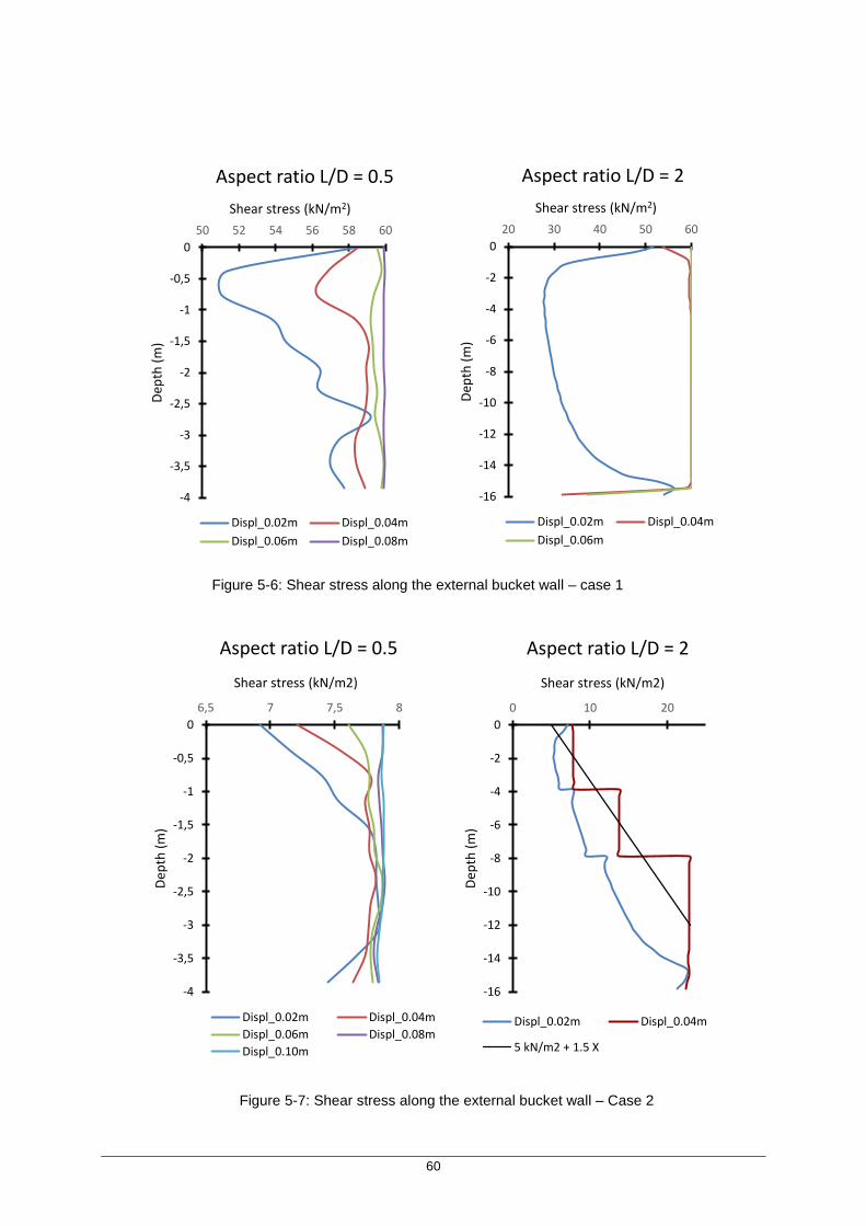
60
Figure 5-6: Shear stress along the external bucket wall – case 1
-4
-3,5
-3
-2,5
-2
-1,5
-1
-0,5
0
50 52 54 56 58 60
Dep
th (
m)
Shear stress (kN/m2)
Aspect ratio L/D = 0.5
Displ_0.02m Displ_0.04m
Displ_0.06m Displ_0.08m
-16
-14
-12
-10
-8
-6
-4
-2
0
20 30 40 50 60
Dep
th (
m)
Shear stress (kN/m2)
Aspect ratio L/D = 2
Displ_0.02m Displ_0.04m
Displ_0.06m
-4
-3,5
-3
-2,5
-2
-1,5
-1
-0,5
0
6,5 7 7,5 8
Dep
th (
m)
Shear stress (kN/m2)
Aspect ratio L/D = 0.5
Displ_0.02m Displ_0.04m
Displ_0.06m Displ_0.08m
Displ_0.10m
-16
-14
-12
-10
-8
-6
-4
-2
0
0 10 20
Dep
th (
m)
Shear stress (kN/m2)
Aspect ratio L/D = 2
Displ_0.02m Displ_0.04m
5 kN/m2 + 1.5 X
Figure 5-7: Shear stress along the external bucket wall – Case 2
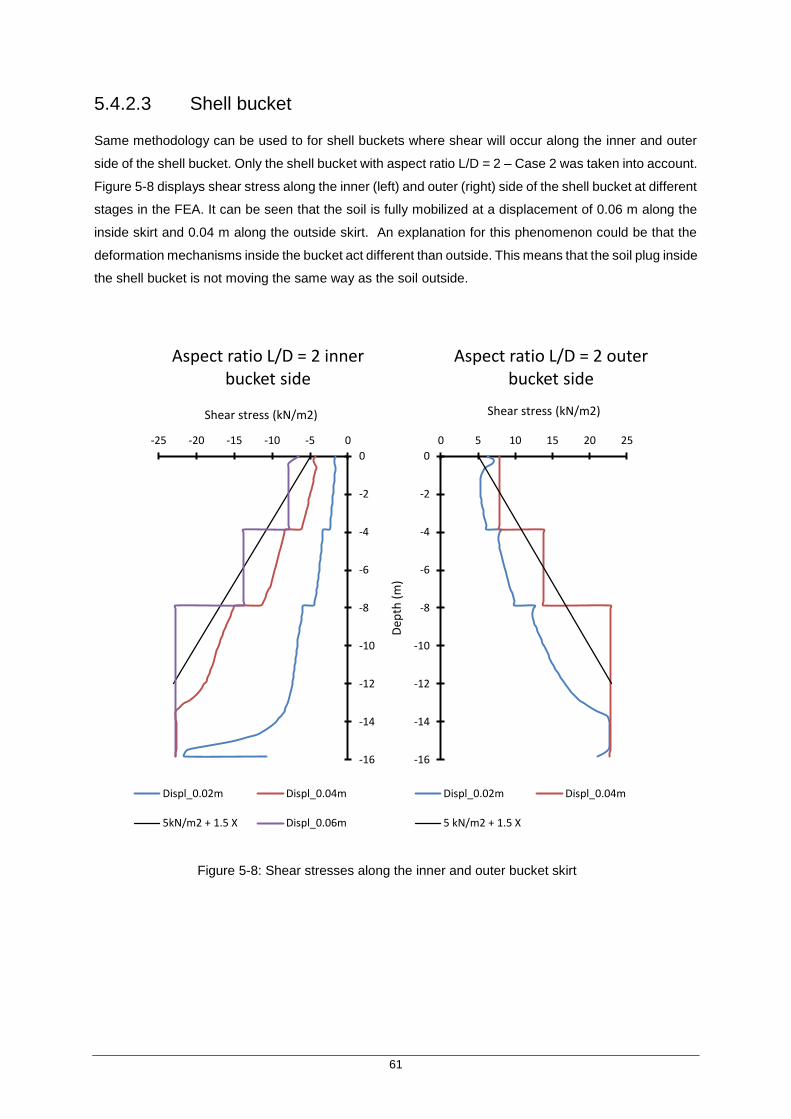
61
5.4.2.3 Shell bucket
Same methodology can be used to for shell buckets where shear will occur along the inner and outer
side of the shell bucket. Only the shell bucket with aspect ratio L/D = 2 – Case 2 was taken into account.
Figure 5-8 displays shear stress along the inner (left) and outer (right) side of the shell bucket at different
stages in the FEA. It can be seen that the soil is fully mobilized at a displacement of 0.06 m along the
inside skirt and 0.04 m along the outside skirt. An explanation for this phenomenon could be that the
deformation mechanisms inside the bucket act different than outside. This means that the soil plug inside
the shell bucket is not moving the same way as the soil outside.
-16
-14
-12
-10
-8
-6
-4
-2
0
0 5 10 15 20 25
Dep
th (
m)
Shear stress (kN/m2)
Aspect ratio L/D = 2 outer bucket side
Displ_0.02m Displ_0.04m
5 kN/m2 + 1.5 X
-16
-14
-12
-10
-8
-6
-4
-2
0
-25 -20 -15 -10 -5 0
Shear stress (kN/m2)
Aspect ratio L/D = 2 inner bucket side
Displ_0.02m Displ_0.04m
5kN/m2 + 1.5 X Displ_0.06m
Figure 5-8: Shear stresses along the inner and outer bucket skirt

62
5.4.3 Load – Displacement analysis and results
5.4.3.1 Analytical calculation of vertical bearing capacity
5.4.3.1.1 Solid bucket
However in this dissertation solid buckets are seen as shallow foundation with resistance at the outer
side of the foundation. The side resistance should then be added to the capacity predicted by the
conventional method in 2.4.2. So this equation is modified by appending the side resistance qs.As .
𝑉𝑢,𝑠𝑜𝑙𝑖𝑑 = 𝑞𝑓 𝐴𝑏 + 𝑞𝑠 𝐴𝑠 (Equation 5.4)
𝑉𝑢,𝑠𝑜𝑙𝑖𝑑 = (𝑁𝑐 ∙ 𝑠𝑢 + 𝛾𝑡 ∙ 𝑑) 𝐴𝑏 + 𝛼 𝑠𝑢 ∙ 𝐷 ∙ 𝑑 ∙ 𝜋 (Equation 5.5)
Where
𝛼 = adhesion factor of the soil
𝛾𝑡 = unite weight of the soil
d = embedment of the bucket
To calculate the undrained failure conditions on the side of a pile or bucket, an adhesion factor is applied
to the undrained shear strength. This factor reflects the alterations that occur at the interface as part of
the installation process of the pile/bucket, that result in a resistance lower than that of the intact
undrained shear strength of the soil. A number of proposals for the variation of adhesion factor in relation
to the intact undrained shear strength are available in the literature, e.g. Figure 5-9.
Figure 5-9: adhesion factor undrained failure condition [49]
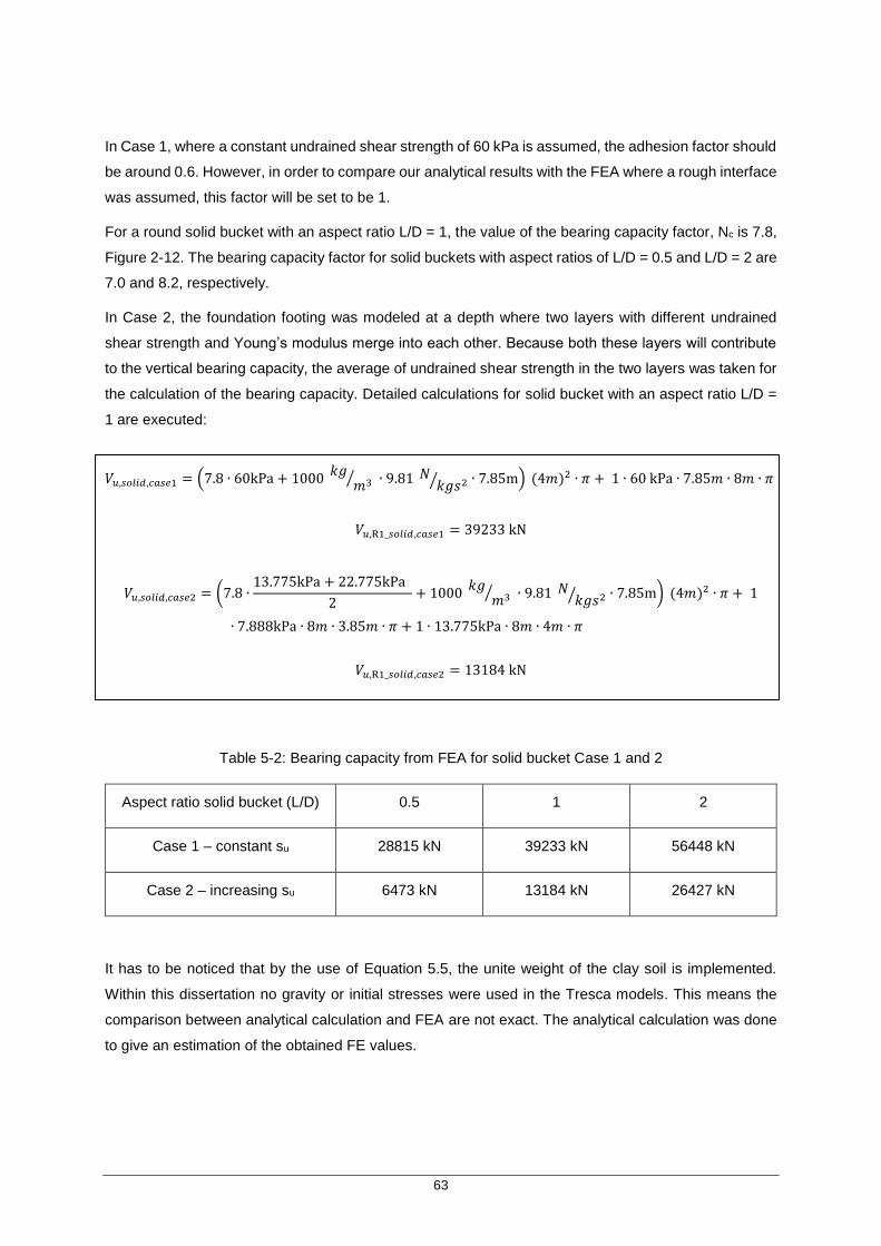
63
In Case 1, where a constant undrained shear strength of 60 kPa is assumed, the adhesion factor should
be around 0.6. However, in order to compare our analytical results with the FEA where a rough interface
was assumed, this factor will be set to be 1.
For a round solid bucket with an aspect ratio L/D = 1, the value of the bearing capacity factor, Nc is 7.8,
Figure 2-12. The bearing capacity factor for solid buckets with aspect ratios of L/D = 0.5 and L/D = 2 are
7.0 and 8.2, respectively.
In Case 2, the foundation footing was modeled at a depth where two layers with different undrained
shear strength and Young’s modulus merge into each other. Because both these layers will contribute
to the vertical bearing capacity, the average of undrained shear strength in the two layers was taken for
the calculation of the bearing capacity. Detailed calculations for solid bucket with an aspect ratio L/D =
1 are executed:
𝑉𝑢,𝑠𝑜𝑙𝑖𝑑,𝑐𝑎𝑠𝑒1 = (7.8 ∙ 60kPa + 1000 𝑘𝑔
𝑚3⁄ ∙ 9.81 𝑁𝑘𝑔𝑠2⁄ ∙ 7.85m) (4𝑚)2 ∙ 𝜋 + 1 ∙ 60 kPa ∙ 7.85𝑚 ∙ 8𝑚 ∙ 𝜋
𝑉𝑢,R1_𝑠𝑜𝑙𝑖𝑑,𝑐𝑎𝑠𝑒1 = 39233 kN
𝑉𝑢,𝑠𝑜𝑙𝑖𝑑,𝑐𝑎𝑠𝑒2 = (7.8 ∙13.775kPa + 22.775kPa
2+ 1000
𝑘𝑔𝑚3⁄ ∙ 9.81 𝑁
𝑘𝑔𝑠2⁄ ∙ 7.85m) (4𝑚)2 ∙ 𝜋 + 1
∙ 7.888kPa ∙ 8𝑚 ∙ 3.85𝑚 ∙ 𝜋 + 1 ∙ 13.775kPa ∙ 8𝑚 ∙ 4𝑚 ∙ 𝜋
𝑉𝑢,R1_𝑠𝑜𝑙𝑖𝑑,𝑐𝑎𝑠𝑒2 = 13184 kN
Table 5-2: Bearing capacity from FEA for solid bucket Case 1 and 2
Aspect ratio solid bucket (L/D) 0.5 1 2
Case 1 – constant su 28815 kN 39233 kN 56448 kN
Case 2 – increasing su 6473 kN 13184 kN 26427 kN
It has to be noticed that by the use of Equation 5.5, the unite weight of the clay soil is implemented.
Within this dissertation no gravity or initial stresses were used in the Tresca models. This means the
comparison between analytical calculation and FEA are not exact. The analytical calculation was done
to give an estimation of the obtained FE values.

64
5.4.3.1.2 Shell bucket
Figure 5-11 explains how the ultimate vertical bearing capacity of shell buckets is mobilized. First the
bucket is assumed to be wished-in-place with a small gap of 0.15m between the soil surface and the
underside of the bucket lid, Figure 5-11 (a). In this model, this gap is assumed to be an empty void,
however this more likely to be a layer of water. As the load increases, the shell bucket will be subjected
to a vertical displacement where the resistance is mainly created in the bucket skirts, Figure 5-11 (b),
as discussed in 5.4.2.1. At a displacement of around 0.15 m, the underside of the bucket lid will touch
the mudline and thus, the bearing capacity will increase subsequently, Figure 5-11 (c). Finally, the
ultimate vertical bearing capacity of the shell bucket is fully mobilized with contributions from the side
and base resistance, Figure 5-11 (d). The total bearing vertical capacity can now be seen as the
summation of the base resistance (Rb), which includes the compressed soil inside the bucket, and the
side resistance (Rs). The load-displacement graph with the different stages to become the end bearing
is shown in Figure 5-12.
It should be noticed that the longer the skirts of the bucket are, the more side resistance is occurring
along the bucket skirts. This means that the assumption of Figure 5-11 is not always true. This particular
phenomenon will be discussed in 5.4.3.2.
𝑉
𝑉
ℎ
ℎ
𝐿
𝑉𝑢,𝑠ℎ𝑒𝑙𝑙
𝑉
𝑅𝑠,𝑜 = 𝜋 ∙ 𝐷𝑜 ∙ 𝐿 ∙ 𝑆𝑢 ℎ
ℎ
𝐿
𝐿
𝑅𝑏 = 𝑁𝑐 ∙ 𝜁𝑠
∙ 𝜁𝑒
∙ 𝐴 ∙ 𝑆𝑢
ℎ
ℎ
𝐿
𝐿
𝐷𝑜
𝑉
𝑉
ℎ
ℎ
𝐿
𝐿
(a)
(b)
(c)
(d)
Figure 5-11: Vertical ultimate bearing capacity
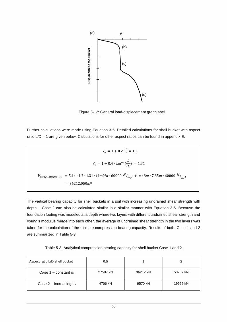
65
Further calculations were made using Equation 3-5. Detailed calculations for shell bucket with aspect
ratio L/D = 1 are given below. Calculations for other aspect ratios can be found in appendix E.
𝜁𝑠 = 1 + 0.2 ∙𝐷
𝐷= 1.2
𝜁𝑒 = 1 + 0.4 ∙ tan−1(𝐿
𝐷𝑜
) = 1.31
𝑉𝑢,𝑠ℎ𝑒𝑙𝑙𝑏𝑢𝑐𝑘𝑒𝑡_𝑅1 = 5.14 ∙ 1.2 ∙ 1.31 ∙ (4𝑚)2𝜋 ∙ 60000 𝑁𝑚2⁄ + 𝜋 ∙ 8𝑚 ∙ 7.85𝑚 ∙ 60000 𝑁
𝑚2⁄
= 36212.050𝑘𝑁
The vertical bearing capacity for shell buckets in a soil with increasing undrained shear strength with
depth – Case 2 can also be calculated similar in a similar manner with Equation 3-5. Because the
foundation footing was modeled at a depth where two layers with different undrained shear strength and
young’s modulus merge into each other, the average of undrained shear strength in the two layers was
taken for the calculation of the ultimate compression bearing capacity. Results of both, Case 1 and 2
are summarized in Table 5-3.
Table 5-3: Analytical compression bearing capacity for shell bucket Case 1 and 2
Aspect ratio L/D shell bucket 0.5 1 2
Case 1 – constant su 27587 kN 36212 kN 50707 kN
Case 2 – increasing su 4706 kN 9570 kN 19599 kN
Dis
pla
cem
en
t to
p B
uck
et
V (a)
(b)
(c)
(d)
Figure 5-12: General load-displacement graph shell
66
5.4.3.2 Results and discussion
In order to check if the results of the FEA are reliable, the results of the 2D and 3D FEA will be compared
with the theoretical calculations that were conducted before. These comparisons are made for
compression and tension loading only, as horizontal loading is not possible in a 2D axisymmetric model.
Furthermore, a comparison between both solid and shell buckets with the same aspect ratios and soil
case will be made in order to examine if both foundations could have the same vertical bearing capacity.
This is an important issue within the offshore foundation industry because by the use of shell buckets
the cost can be reduced in terms of materials and installation time compared to solid buckets, which can
be compared to gravity foundations.
Finally, the theory of the reverse bearing capacity for shell buckets is examined for all aspect ratios and
soil cases and subsequently discussed.
5.4.3.2.1 Compression
As mentioned in the introduction, the analyses using solid buckets are discussed first. In Figure 5-13
the load displacement response for solid buckets with L/D ratios of 0.5, 1 and 2, for both Case 1 –
constant undrained shear strength and Case 2 – increasing undrained shear strength are presented.
An increase of load on the top of the solid bucket will be accompanied by an increase of settlement. The
response is approximately linear (elastic) at the beginning of loading until about 45% of the axial
resistance is mobilized. Loads applied in this area causes only small displacement and are most of the
time reversible. After a bend in the load-displacement curve, the rate of increase in the resistance
reduces significantly. At a relatively large displacement of 0.35 m, the increase in resistance becomes
insignificant and the ultimate bearing load is approached. A further increase of the load will be
accompanied with a large increase of the settlement by which failure of the soil will occur.
It can be seen that the soil in Case 1 gives a greater vertical bearing capacity because of the greater
undrained shear strength on the depth of the footing and on the side of the foundation. For example, in
Case 1, a solid bucket with L/D = 1 (R1), reached an ultimate bearing load of 39233 kN whereas in Case
2 the same bucket reached an ultimate load of only 13184 kN
The vertical lines in the graph represent the analytical results of the calculation for vertical bearing
capacity. These values were evaluated in order to give an estimation of the achieved ultimate vertical
bearing load.

67
Secondly, shell buckets were considered. As seen in Figure 5-14 – Case 1, the resistance of the bucket
with an aspect ratio L/D = 0.5 initially plateaus as the side resistance is fully mobilized and then at a
displacement of about 0.15 m the gap closes and a further increase in resistance is mobilized.
Examining the load-displacement graph for the bucket with L/D =1 (R1), the leap in the curve seems to
flatten off and for L/D = 2 (R2) is absent. This can be explained by the length of the bucket skirts; the
longer the skirts are, the more friction will occur along the inside of the bucket. Deeper embedment of
the skirts induces more vertical capacity attributable to the mobilization of the adhesion. As seen in
Figure 5-15, the deformed mesh for bucket aspect ratio L/D =2 (R2) shows that the gap configuration
will stay more or less in place moving soil and bucket downwards (plugging). Further explanation of this
phenomenon will be discussed in Figure 5-16.
It also has to be noticed that this effect depends on the undrained shear strength of the clay soil. In Case
2, it is seen that bucket lid of ratio L/D = 2 will touch the mudline and thus the bearing capacity will
increase subsequently.
Most of the FEA results are acceptable when compared to the theoretical solutions for bearing capacity.
The vertical lines in the graph represent the analytical bearing capacity results from Table 5-3.
-0,35
-0,3
-0,25
-0,2
-0,15
-0,1
-0,05
0
0 10000 20000 30000 40000 50000 60000
Dis
pla
cem
en
t To
p B
uck
et
(m)
Load (kN)
Vertical bearing capacity Solid Buckets - Case 1
R0.5 R1 R2
Theory_R0.5 Theory_R1 Theory_R2
-0,35
-0,3
-0,25
-0,2
-0,15
-0,1
-0,05
0
0 5000 10000 15000 20000 25000 30000
Dis
pla
cem
en
t To
p B
uck
et
(m)
Load (kN)
Vertical bearing capacity Solid Buckets - Case 2
R0.5 R1 R2
Theory_R0.5 Theory_R1 Theory_R2
Figure 5-13: Vertical compression bearing capacity solid bucket - Case 1 and 2

68
Differences between numerical results and theoretically calculation for Case 1 range between 0.38%
and 6.4% and for Case 2 between 2.3% and 30%. The 30% difference was for the bucket with an aspect
ratio of 0.5 and is an outliner compared to all other results. No explanation was found for this result.
-0,3
-0,25
-0,2
-0,15
-0,1
-0,05
0
0 10000 20000 30000 40000 50000
Dis
pla
cem
en
t to
p b
uck
et
(m)
Load (kN)
Vertical bearing capcity Shell Buckets - Case 1
R0.5 R1 R2
Theory_R0.5 Theory_R1 Theory_R2
-0,3
-0,25
-0,2
-0,15
-0,1
-0,05
0
0 5000 10000 15000 20000
Dis
pla
cem
en
t to
p b
uck
et
(m)
Load (kN)
Vertical bearing capacity Shell Bucket - Case 2
R0.5 R1 R2
Theory_R0.5 Theory_R1 Theory_R2
Figure 5-14: Compression bearing capacity shell buckets - Case 1 and 2
Figure 5-15: Undefromed (transparent) and deformed (green) mesh after displacement of 0.15m - R1 (left)
and R2 (right)
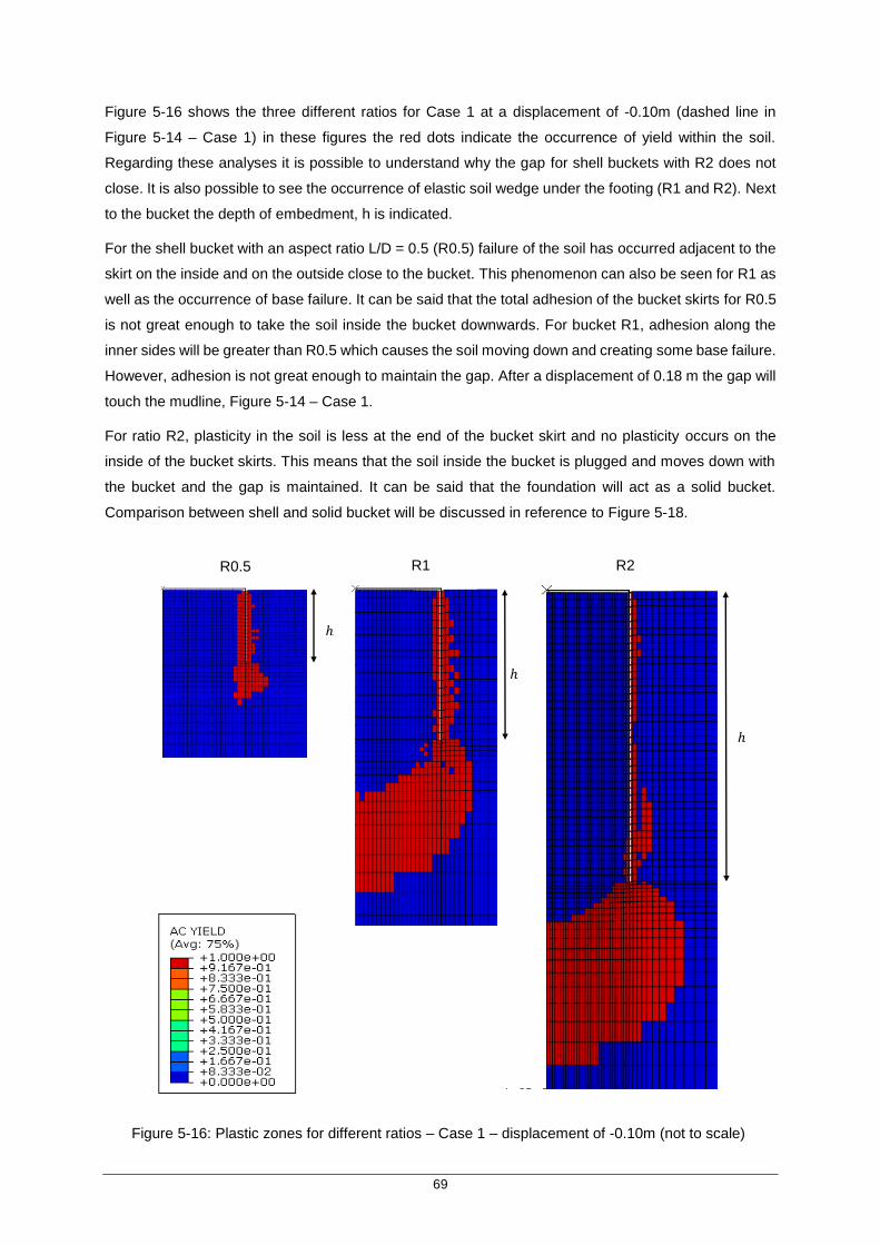
69
Figure 5-16 shows the three different ratios for Case 1 at a displacement of -0.10m (dashed line in
Figure 5-14 – Case 1) in these figures the red dots indicate the occurrence of yield within the soil.
Regarding these analyses it is possible to understand why the gap for shell buckets with R2 does not
close. It is also possible to see the occurrence of elastic soil wedge under the footing (R1 and R2). Next
to the bucket the depth of embedment, h is indicated.
For the shell bucket with an aspect ratio L/D = 0.5 (R0.5) failure of the soil has occurred adjacent to the
skirt on the inside and on the outside close to the bucket. This phenomenon can also be seen for R1 as
well as the occurrence of base failure. It can be said that the total adhesion of the bucket skirts for R0.5
is not great enough to take the soil inside the bucket downwards. For bucket R1, adhesion along the
inner sides will be greater than R0.5 which causes the soil moving down and creating some base failure.
However, adhesion is not great enough to maintain the gap. After a displacement of 0.18 m the gap will
touch the mudline, Figure 5-14 – Case 1.
For ratio R2, plasticity in the soil is less at the end of the bucket skirt and no plasticity occurs on the
inside of the bucket skirts. This means that the soil inside the bucket is plugged and moves down with
the bucket and the gap is maintained. It can be said that the foundation will act as a solid bucket.
Comparison between shell and solid bucket will be discussed in reference to Figure 5-18.
R0.5 R1 R2
ℎ
ℎ
ℎ
Figure 5-16: Plastic zones for different ratios – Case 1 – displacement of -0.10m (not to scale)
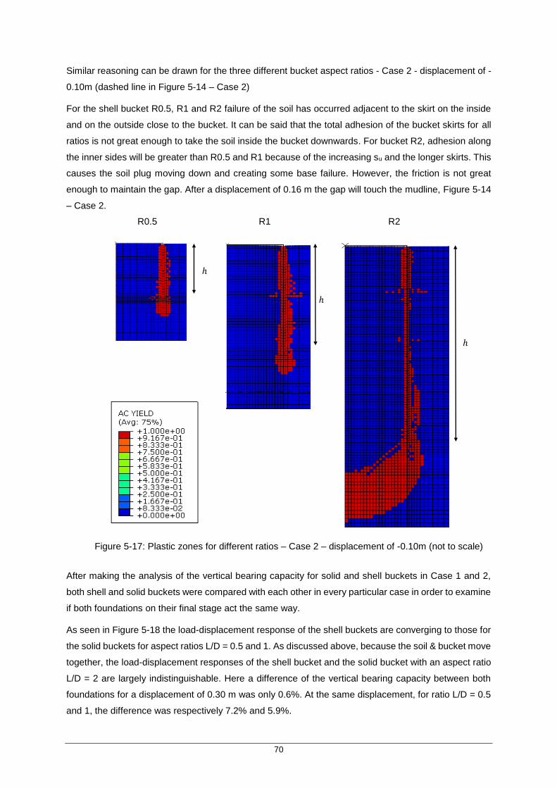
70
Similar reasoning can be drawn for the three different bucket aspect ratios - Case 2 - displacement of -
0.10m (dashed line in Figure 5-14 – Case 2)
For the shell bucket R0.5, R1 and R2 failure of the soil has occurred adjacent to the skirt on the inside
and on the outside close to the bucket. It can be said that the total adhesion of the bucket skirts for all
ratios is not great enough to take the soil inside the bucket downwards. For bucket R2, adhesion along
the inner sides will be greater than R0.5 and R1 because of the increasing su and the longer skirts. This
causes the soil plug moving down and creating some base failure. However, the friction is not great
enough to maintain the gap. After a displacement of 0.16 m the gap will touch the mudline, Figure 5-14
– Case 2.
After making the analysis of the vertical bearing capacity for solid and shell buckets in Case 1 and 2,
both shell and solid buckets were compared with each other in every particular case in order to examine
if both foundations on their final stage act the same way.
As seen in Figure 5-18 the load-displacement response of the shell buckets are converging to those for
the solid buckets for aspect ratios L/D = 0.5 and 1. As discussed above, because the soil & bucket move
together, the load-displacement responses of the shell bucket and the solid bucket with an aspect ratio
L/D = 2 are largely indistinguishable. Here a difference of the vertical bearing capacity between both
foundations for a displacement of 0.30 m was only 0.6%. At the same displacement, for ratio L/D = 0.5
and 1, the difference was respectively 7.2% and 5.9%.
ℎ
ℎ
ℎ
R0.5 R1 R2
Figure 5-17: Plastic zones for different ratios – Case 2 – displacement of -0.10m (not to scale)

71
The same scenario as seen for Case 1 is also occurring for Case 2; the load-displacement response of
the three shell buckets converge towards those for the solid buckets. The main difference between Case
1 and 2 is the lower load-bearing capacity and the lower amount of adhesion along the inner skirts of
the buckets due to the lower undrained strength of the clay soil in the latter. Where in Case 1 a bucket
with an aspect ratio L/D = 2 almost entirely acted as a solid bucket, in Case 2 there is failure of the soil
inside the bucket, plugging does not occur and the load-displacement curve will converge to the solid
bucket case.
The difference of the vertical bearing capacity between both foundations for a displacement of 0.30 m
for the aspect ratios L/D = 0.5, 1 and 2 were 2.2%, 9.0% and 5.6% respectively.
It has to be noticed that the comparison between both foundation types are within the FEA and only
simplified models were taken into account. In practice, parameters like time, consolidation, water
pressure, deforming of the steel and many more parameters must also be considered while modelling.
-0,3
-0,25
-0,2
-0,15
-0,1
-0,05
0
0 10000 20000 30000 40000 50000
Dis
pla
cem
en
t to
p b
uck
et
(m)
Load (kN)
Comparison vertical bearing capacity solid and shell bucket - case 1
2D_shellbucket_R0.5 2D_shellbucket_R1
2D_shellbucket_R2 2D_Solidbucket_R0.5
2D_Solidbucket_R1 2D_Solidbucket_R2
-0,3
-0,25
-0,2
-0,15
-0,1
-0,05
0
0 5000 10000 15000 20000
Dis
pla
cem
en
t to
p b
uck
et
(m)
Load (kN)
Comparison vertical bearing capacity solid and shell bucket - case 2
2D_shellbucket_R1 2D_shellbucket_R05
2D_shellbucket_R2 2D_Solidbucket_R0.5
2D_Solidbucket_R1 2D_Solidbucket_R2
Figure 5-18: Comparison vertical bearing capacity solid and shell bucket - Case 1 & 2

72
5.4.3.2.2 Reverse bearing capacity shell buckets
In order to simulate particular problem of the reverse bearing capacity in ABAQUS, the three shell bucket
configurations – Case 1 soil conditions were also modelled without a gap and with a “tied” constraint
between the bucket lid and the soil. When a tension load is applied to the shell bucket, the soil inside
the bucket remains attached to the bucket lid and follows the displacement of the structure, representing
the passive suction in undrained condition at the bottom of the bucket, Figure 5-19.a. This assertion can
be done because a great amount of capacity will arise after applying tension to the structure, this in
undrained (short-term) conditions. Friction between outer bucket skirt also contributes to the failure
tension load.
Also the shell bucket with gap was used and subjected to a tension load, Figure 5-19.b. Here no “tied”
constraint was used between lid and soil because of the gap. These analysis were done to provide a
lower bound to the undrained tension resistance where passive suction should not occur or rather not
develop the full resistance implied by undrained reverse bearing capacity failure.
As seen in Figure 5-20, the “tension R0.5” and “tension R1” curves with gap formation have practically
the same capacity as the compression case prior to gap closing. This was predictable as the total
resistance is obtained by the friction between skirt and soil, and the friction will be the same in tension
and compression.
Figure 5-19: Vector displacement after applying a tension load on shell bucket R0.5 with
a) no gap configuration and b) gap configuration
a. b.

73
For the “tension R2” Case, as in the compression case, because of the length of the shell bucket skirt,
the soil inside the bucket moves with the bucket. The side friction mobilised for this bucket aspect ratio
is sufficient to allow the formation of a reverse bearing capacity effect and the load-displacement
response is indistinguishable from the compression Case.
The dashed lines in Figure 5-20 represent the no gap shell bucket configurations where the lid is tied to
the soil. Comparing the result for these analyses with the equivalent compression case, it can be seen
that failure mode of the shell bucket subjected to an uplifting load under undrained conditions may be
considered a reverse bearing capacity mechanism as discussed in Section 3.5.3. However, as
mentioned before, these assumptions are purely theoretical and offshore design standards for shallow
foundations do not allow the vertical pull-out resistance due to suction between soil and bucket lid to be
utilized. These analyses involved a major simplification of the mechanism, if the suction effect would
have been implemented, the model had to be coupled like [29].
-0,3
-0,25
-0,2
-0,15
-0,1
-0,05
0
0,05
0,1
0,15
0,2
0 5000 10000 15000 20000 25000 30000 35000 40000 45000 50000
Dis
pla
cem
en
t to
p b
uck
et
(m)
Load (kN)
Reverse bearing mechanism shell bucket - Case 1
Tension R0.5 Tension R1 Tension R2
compression R0.5 compression R1 compression R2
No Gap Tension R0.5 No gap tension R1 No gap tension R2
Figure 5-20: Reverse bearing capacity shell buckets
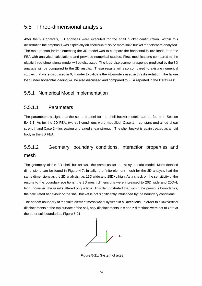
74
5.5 Three-dimensional analysis
After the 2D analysis, 3D analyses were executed for the shell bucket configuration. Within this
dissertation the emphasis was especially on shell bucket so no more solid bucket models were analysed.
The main reason for implementing the 3D model was to compare the horizontal failure loads from the
FEA with analytical calculations and previous numerical studies. First, modifications compared to the
elastic three-dimensional model will be discussed. The load-displacement response predicted by the 3D
analysis will be compared to the 2D results. These results will also compared to existing numerical
studies that were discussed in 0, in order to validate the FE-models used in this dissertation. The failure
load under horizontal loading will be also discussed and compared to FEA reported in the literature 0.
5.5.1 Numerical Model implementation
5.5.1.1 Parameters
The parameters assigned to the soil and steel for the shell bucket models can be found in Section
5.4.1.1. As for the 2D FEA, two soil conditions were modelled; Case 1 – constant undrained shear
strength and Case 2 – increasing undrained shear strength. The shell bucket is again treated as a rigid
body in the 3D FEA.
5.5.1.2 Geometry, boundary conditions, interaction properties and
mesh
The geometry of the 3D shell bucket was the same as for the axisymmetric model. More detailed
dimensions can be found in Figure 4-7. Initially, the finite element mesh for the 3D analysis had the
same dimensions as the 2D analysis, i.e. 15D wide and 15D+L high. As a check on the sensitivity of the
results to the boundary positions, the 3D mesh dimensions were increased to 20D wide and 20D+L
high; however, the results altered only a little. This demonstrated that within the previous boundaries,
the calculated behaviour of the shell bucket is not significantly influenced by the boundary conditions.
The bottom boundary of the finite element mesh was fully fixed in all directions. In order to allow vertical
displacements at the top surface of the soil, only displacements in x and z directions were set to zero at
the outer soil boundaries, Figure 5-21.
Figure 5-21: System of axes

75
The interface interaction properties applied were the same as in the 2D analysis but divided in different
interface sets. This was done to decrease the arithmetical effort of the models.
In the 3D elastic model, two element types were used, six node triangular prisms and eight node brick
elements. However, it seems that six node triangular prism elements are not very well suited for FEA
unless a lot of them are used and so the model was modified so that eight node elements could be used
to represent the ground within the bucket, Figure 5-22. If no mesh optimization was done, a difference
for the ultimate vertical capacity of more than 25% between 2D and 3D FEA occurred; this reduced to
2% with the new mesh.
5.5.2 Load – Displacement results and discussion
5.5.2.1 Comparison 2D and 3D FEA
In order to validate the 3D models, the load-displacement results were compared with those from the
2D analysis. As seen in Figure 5-23, the differences between the 2D and 3D analyses are negligible
with both curves almost coinciding. The differences between the 2D and 3D results for R0.5, R1 and R2
at a penetration depth of 0.3 m, are 2.01 %, 1.11% and 0.06% respectively.
These small differences are thought to be largely due to the use of different element types in the models
and perhaps the grading of the finite element mesh. It should be noted that as a consequence of the
close agreement in the results, the conclusions drawn from the 2D FEA in also apply to the 3D FEA
results.
Figure 5-22: Mesh configuration: C3D8
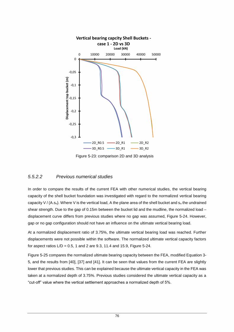
76
5.5.2.2 Previous numerical studies
In order to compare the results of the current FEA with other numerical studies, the vertical bearing
capacity of the shell bucket foundation was investigated with regard to the normalized vertical bearing
capacity V / (A.su). Where V is the vertical load, A the plane area of the shell bucket and su the undrained
shear strength. Due to the gap of 0.15m between the bucket lid and the mudline, the normalized load –
displacement curve differs from previous studies where no gap was assumed, Figure 5-24. However,
gap or no gap configuration should not have an influence on the ultimate vertical bearing load.
At a normalized displacement ratio of 3.75%, the ultimate vertical bearing load was reached. Further
displacements were not possible within the software. The normalized ultimate vertical capacity factors
for aspect ratios L/D = 0.5, 1 and 2 are 9.3, 11.4 and 15.9, Figure 5-24.
Figure 5-25 compares the normalized ultimate bearing capacity between the FEA, modified Equation 3-
5, and the results from [40], [37] and [41]. It can be seen that values from the current FEA are slightly
lower that previous studies. This can be explained because the ultimate vertical capacity in the FEA was
taken at a normalized depth of 3.75%. Previous studies considered the ultimate vertical capacity as a
“cut-off” value where the vertical settlement approaches a normalized depth of 5%.
-0,3
-0,25
-0,2
-0,15
-0,1
-0,05
0
0 10000 20000 30000 40000 50000
Dis
pla
cem
en
t to
p b
uck
et
(m)
Load (kN)
Vertical bearing capcity Shell Buckets -case 1 - 2D vs 3D
2D_R0.5 2D_R1 2D_R2
3D_R0.5 3D_R1 3D_R2
Figure 5-23: comparison 2D and 3D analysis

77
0
2
4
6
8
10
12
14
16
18
0 0,5 1 1,5 2 2,5 3 3,5 4
V/(
A*S
u)
displacement/D %R05 R1 R2
Figure 5-24: Case 1 - Normalized vertical load-displacement curve, bucket with gap
Figure 5-25: Comparison normalized ultimate vertical-displacement curve
6
8
10
12
14
16
18
0 0,5 1 1,5 2 2,5
Vu
lt/(
A*S
u)
Ratio L/D
FEA (This work) Mod. Equation 3.5
FEA by Yun-gang et al. FEA by Le chi Hung et al.
FEA by H.A Taiebat et al.

78
5.5.3 Horizontal capacity analysis
Horizontal load analyses were executed considering loads applied to the top of the shell bucket. Here
two scenarios were considered; first, no rotation of the bucket lid was allowed, and secondly, free
rotation of the shell bucket was allowed.
5.5.3.1 Analytical results
Case 1 - constant undrained shear strength was taken to calculate ultimate horizontal capacity for purely
horizontal displacements. The lateral bearing capacity factor Np was estimated to be 9.5, 10 and 10 for
respectively the ratios L/D =0.5, 1 and 2, Figure 3-7. Detailed calculations for the ultimate horizontal
capacity can be found in Appendix F.
Where Hult = L.D0.Np.su can only be used for pure lateral translation, no approximation for ultimate
horizontal capacities for shell bucket where the rotation was allowed were found. Failure modes of shell
buckets subjected to a horizontal load on the top of the bucket where rotation is allowed can be similar
treated to those for laterally loaded piles [10]. However, this theory cannot be used within this
dissertation because of the use of rigid body constraint.
5.5.3.2 Results and discussion
As seen in Figure 5-26, the lateral bearing capacity factor for horizontal load, with and without the
allowance of rotation, in soils with uniform undrained shear strength, gained from FEA is acceptable
compared with theoretical assumptions.
Figure 5-27 shows the normalized horizontal bearing capacity for the different aspect ratios L/D when
rotation is allowed. The normalized ultimate horizontal capacity Hult / (A.su) for each aspect ratio can
now be obtained from this figure. For aspect ratio L/D = 0.5, 1 and 2 the normalized ultimate horizontal
capacity is 4.5, 5.8 and 9.6 respectively. Compared to previous studies in 0, these values are acceptable.

79
Figure 5-28 shows the vector displacement failure mechanism under purely horizontal load (a) and
horizontal load with allowance of rotation (b) for aspect ratio L/D = 2.
0
2
4
6
8
10
12
0 1 2 3 4 5
Hu
lt /
(L*D
*Su
) =
Np
Ratio L/DUniform Su_purely horizontal translation
Uniform Su_rotation allowed
0
2
4
6
8
10
12
0 0,002 0,004 0,006 0,008 0,01 0,012 0,014 0,016 0,018
Ho
rizo
nta
l Lo
ad/(
A*S
u)
u/D
R05 R1 R2
Figure 5-26: lateral bearing capacity factor Np in function of the aspect ratios L/D
Figure 5-27: Normalized horizontal bearing capacity with rotation for different
aspect ratios.
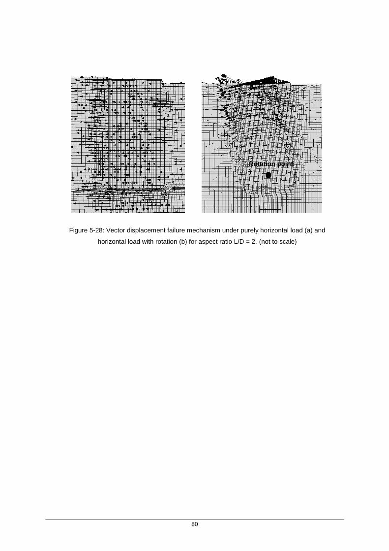
80
Figure 5-28: Vector displacement failure mechanism under purely horizontal load (a) and
horizontal load with rotation (b) for aspect ratio L/D = 2. (not to scale)
Rotation point
81
Chapter 6
Conclusions
6 Conclusions
The current thesis intended to analyse in a systematic way the behaviour of shell bucket foundation
structures. The main results of numerical study on the bearing capacity and conclusions are summarized
in this chapter.

82
6.1 Summary and Conclusions
Bucket foundations for offshore wind turbines under vertical and horizontal loads were investigated using
FEA, considering the frictional contact of the interface between structure and sub-soil. The results were
obtained from 2D and 3D numerical analyses of solid and shell bucket foundations in homogeneous
clay soil which deforms under undrained conditions. This means that only total stress analysis was
carried out and pore water pressure was disregarded while modelling. Displacement-load controlled
method was used to predict the “cut-off” value of vertical capacity and load-displacement controlled
method was used to derive the ultimate horizontal capacity.
To become a fully operational Tresca model in chapter 5, first a total elastic model was implemented. In
Chapter 4, the linear elastic behaviour of solid and shell bucket was discussed. The following
conclusions that were drawn from this chapter:
For a solid bucket configuration acting as a shallow foundation, the relative settlement
differences between 2D FEA and 3D FEA compared with analytical calculations for all aspect
ratios varied from 7 % to 20 %.
The differences in predicted settlements between 2D and 3D solid bucket configurations vary
from 1 % to 4 %
The differences in predicted settlements between 2D and 3D shell bucket configurations are
around 10%
It should be noted that the mesh in this model was subjected to some change. While the differences
between analytical calculations were acceptable in the elastic model, differences for displacement –
load control of more than 20% arose in the Tresca model. The models for the elastic configuration were
not re-run with the modified mesh because the main purpose of this dissertation was to obtain a good
working Tresca model.
In Chapter 5, the results of analytical calculations for the ultimate vertical bearing capacity for shell
buckets were compared with the 2D- axisymmetric FEA. Furthermore, detailed analysis were executed
to understand the plastic behaviour of the soil near the skirt edges and at the footings of the foundation.
The latter was preformed to understand the conservation of the gap between bucket lid and seafloor
when the shell bucket is subjected to a compression load. Next, a comparison was done between solid
and shell bucket FEA in order to examine if both foundations types could have the same ultimate vertical
capacity. Finally, the theory of reverse bearing mechanism was evaluated and compared with the results
of FEA. Based on these series of numerical analyses, the following conclusions can be drawn:
The vertical capacity for FEA for shell buckets agrees well with the modified conventional
method considering the add-in of the adhesion between the shell bucket skirts and the subsoil.
The longer the skirts are, the more adhesion will develop along the skirt edges which ensures
that the soil plug inside the bucket will be subjected to a downwards movement together with

83
the foundation structure. Because the total adhesion along the skirts depends on the
undrained shear strength of the soil, the preservation of the gap will also be dependent on su.
The assumption, that the ultimate vertical bearing capacity for each particular aspect ratio for
solid and shell buckets will approximately be the same, was confirmed. Based on FEA,
differences at a “cut-off displacement” of 0.30 m between solid and shell buckets ranged
between 1% and 9%. Here, the shell buckets showed a slightly lower ultimate vertical
resistance in all cases.
To prove the reverse bearing capacity in undrained conditions (short-term), shell buckets, with
no gap configurations between bucket lid and seafloor, were subjected to a tension load.
Comparing the result for these analyses with equivalent compression case, failure mode for
shell buckets subjected to a tension load may be considered as a reverse bearing mechanism.
However, in practical terms, no design guidelines take this theory in consideration as it is only
valid for short-term problems.
Because it is not possible to model horizontal loads in a 2D analysis, 3D shell bucket models were
developed to compare horizontal failure from FEA with theoretical assumptions and previous numerical
studies. First, in order to validate these 3D models, the axial load-displacement response predicted by
the 3D FEA was compared to the 2D results. Thereafter, the load-displacement response was
investigated in terms of the normalized vertical bearing capacity and compared with previous studies.
Finally, horizontal capacity analyses were executed with the regard to purely horizontal and horizontal
analysis with the allowance of rotation. The following conclusions that were drawn from the 3D FEA:
Differences between 2D and 3D analyses are negligible. As a consequence of these results,
conclusions drawn from the 2D FEA can also be applied to 3D FEA.
Despite the fact that no displacement greater than normalized depth of 3.75% was possible
within the software, gained values of the normalized ultimate vertical capacity were acceptable
compared to previous studies where the values of the normalized capacity were taken at a
normalized depth of 5%. Eventually, this resulted in slightly smaller values of the normalized
ultimate vertical capacity.
Horizontal capacity under pure translation will be greater than the horizontal capacity with the
allowance of rotation.
When rotation is allowed in soils with uniform undrained shear strength, the lateral bearing
capacity factor Np decreases with the increase of the aspect ratio. When aspect ratio L/D > 2
this effect appears to be stabilizing to a value of around 4. When no rotation is allowed Np
varies between 9 and 10
The normalized ultimate horizontal capacity for FEA agrees well with previous studies.

84
6.2 Further research
Before 2002, bucket foundations were a “blank spot” on the map for offshore wind energy [49]. After a
five-year research program, this novel principle of foundation for offshore wind turbines were proven to
be feasible in suitable soil conditions [50]. Thereafter, more and more research was done by companies
like Dong and Universal Foundations (UF).
Further research that is possible for this particular foundation type:
The undoing of the rigid body constraint for the bucket foundation. Within this thesis a
simplified model was used and presumed to work as a rigid body. If this is not the case,
stiffeners along the bucket skirts and on the bucket lid will be necessary to become an
operational model.
Now the soil configuration was divided in two different cases, constant undrained shear
strength and increasing undrained shear strength. The latter was separated into layers
because of the non-existence of input of increasing undrained shear strength in ABAQUS.
Plaxis, another FE-program, does have this feature.
Modelling the soil with Drucker-Prager yield criterion to determine whether the material has
failed or undergone plastic yielding. This yield criterion for soils has been used in many soil
plasticity problems.
As we presume the bucket is rigid no comparison between piles are available only one
particular case. One of the limiting cases for piles is that the pile behaves as a short rigid
inclusion. A comparison between both pile and bucket would be interesting.
Greater mesh refinement in order to obtain more precise results. However, in three-
dimensional configurations the running-time for one model varied from 15 to 18 hours. By
taking a finer mesh, more elements will be created and running-time will increase.

85
References References [1] REN21. (2014). Renewables 2014 – Global status report (1st ed.). Retrieved from REN21
website:
http://www.ren21.net/portals/0/documents/resources/gsr/2014/gsr2014_full%20report_low%20
res.pdf
[2] COMMUNICATION FROM THE COMMISSION TO THE EUROPEAN PARLIAMENT, THE
COUNCIL, THE EUROPEAN ECONOMIC AND SOCIAL COMMITTEE AND THE COMMITTEE
OF THE REGIONS Energy 2020 A strategy for competitive, sustainable and secure energy
[3] Thayer, R. L., & Freeman, C. M. (1987). Altamont: public perceptions of a wind energy
landscape. Landscape and urban planning, 14, 379-398.
[4] Wind Energy the facts (2011). "Projecting targets for the EU-27 up to 2030." Chapter 2. Website:
http://www.wind-energy-the-facts.org/index-73.html
[5] Implementation of a 2MW Deep Offshore Wind Demonstration Project. (2013, July). Paper
presented at The WindFloat Project- Public Session of edp, Apúlia.
[6] IRENA, I. (2012). Renewable energy technologies: Cost analysis series.Concentrating solar
power.
[7] ORECCA. (2011). WP3 Technologies stat of the art (Final version). Retrieved from ORECCA
website: http://www.orecca.eu/c/document_library/get_file?uuid=144f87d6-c41a-4a04-8742-
7ebdc88f5a5c&groupId=10129
[8] Randolph, M., & Gourvenec, S. (2011). Offshore geotechnical engineering: CRC Press
[9] Den Boon, J., Sutherland, J., Whitehouse, R., Soulsby, R., Stam, C., Verhoeven, K., . . . Hald,
T. (2004). Scour behaviour and scour protection for monopile foundations of offshore wind
turbines. Paper presented at the Proceedings 2004 European Wind Energy Conference,
London, UK. European Wind Energy Association.
[10] Yanguas Miñambres, Ó. (2012). Assessment of current offshore wind support structures
concepts: challenges and technological requirements by 2020.
[11] De Vries, W., Vemula, N. K., Passon, P., Fischer, T., Kaufer, D., Matha, D., . . . Vorpahl, F.
(2011). Final report WP 4.2: Support Structure Concepts for Deep Water Sites: Deliverable D4.
2.8 (WP4: offshore foundations and support structures): Upwind.
[12] 4Coffshore- Jacket or lattice structures (2015). Retrieved from
http://www.4coffshore.com/windfarms/jacket-or-lattice-structures-aid271.html
[13] Randolph, M., Cassidy, M., Gourvenec, S., & Erbrich, C. (2005, September). Challenges of
offshore geotechnical engineering. In Proceedings of the International Conference on Soil
Mechanics and Geotechnical Engineering (Vol. 16, No. 1, p. 123). AA BALKEMA PUBLISHERS.

86
[14] Carrington, D. (2013, January 22). 'Suction bucket' lays new foundation for ofshore wind.
Retrieved form http://www.theguardian.com/environment/2013/jan/22/suction-bucket-offshore-
wind
[15] Peire, K., Nonneman, H., & Bosschem, E. (2009). Gravity base foundations for the thornton
bank offshore wind farm. Terra et Aqua, 115, 19-29.
[16] Humpheson, C. 1998. Foundation design of Wandoo B concrete gravity structure. Offshore Site
Investigation and Foundation Behaviour, Soc. For Underwater Technology, 353-367.
[17] Sturm, H. (2009). Stabilisation behaviour of cyclically loaded shallow foundations for offshore
wind turbines. KIT Scientific Publishing.
[18] Ibsen, L. B., Liingaard, S., & Nielsen, S. A. (2005). Bucket Foundation, a status. Proceedings of
the Copenhagen Offshore Wind.
[19] Winterkorn, H. F., & Fang, H. Y. (1975). Foundation engineering handbook.
[20] Canadian Geotechnical Society. Foundations Committee. (1978). Canadian foundation
engineering manual. Canadian geotechnical society.
[21] Ce-ref (2/15/2009). "Terzaghi's Bearing Capacity Equations." Website:
https://hamidomer.files.wordpress.com/2010/09/terzaghi.pdf
[22] NovoPile User-s Manual (2011). “Nc Parameter undrained condtions.” Website:
http://help.novotechsoftware.com/en/novopile/Nc.htm
[23] Environmetal. ‘Bearing capacity” Website:
http://environment.uwe.ac.uk/geocal/foundations/founbear.htm
[24] (2012). "RE Technologies Cost Analysis Wind Power." IRENA 2012 Volume 1: power sector
(5/5). Website:
https://www.irena.org/DocumentDownloads/Publications/RE_Technologies_Cost_Analysis-
WIND_POWER.pdf
[25] Knowles, V. R. (1991). Settlement of Shallow Footings on Sand: Report and User's Guide for
Computer Program CSANDSET (No. WES/TR/ITL-91-1). ARMY ENGINEER WATERWAYS
EXPERIMENT STATION VICKSBURG MS INFORMATION TECHNOLOGY LAB.
[26] Van Der Tempel, J. (2006). Design of support structures for offshore wind turbines. TU Delft,
Delft University of Technology.
[27] Ce-ref (2009). "Terzaghi's Bearing Capacity Equations." Website: http://www.ce-
ref.com/Foundation/Bearing%20capacity/Terzaghi.html
[28] Sgardeli, C. G. (2009). A finite element analysis of the pullout capacity of suction caissons in
clay (Doctoral dissertation, Massachusetts Institute of Technology).
[29] Deng, W., & Carter, J. P. (2002). A theoretical study of the vertical uplift capacity of suction
caissons. International Journal of Offshore and Polar Engineering, 12(2), 89-97.

87
[30] Acosta-Martinez, H. E., Gourvenec, S. M., & Randolph, M. F. (2010). Effect of gapping on the
transient and sustained uplift capacity of a shallow skirted foundation in clay. Soils and
foundations, 50(5), 725-735.
[31] Randolph, M., & Gourvenec, S. (2011). Offshore geotechnical engineering. CRC Press.
[32] Forewind. (2015). Dogger Bank Creyke Beck. Retrieved from
http://www.forewind.co.uk/projects/dogger-bank-creyke-beck.html
[33] Carrington, D. (2013, January 22). 'Suction bucket' lays new foundation for ofshore wind.
Retrieved form http://www.theguardian.com/environment/2013/jan/22/suction-bucket-offshore-
wind
[34] Bakmar, C. L. "Recent experience and challenges ahead." Dong Energy. Website:
http://www.gl-group.com/pdf/No12_Bakmar.pdf
[35] Romp, R. H. (2013). Installation-effects of suction caissons in non-standard soil
conditions (Doctoral dissertation, TU Delft, Delft University of Technology)
[36] Dong Energy. (2013). The suction bucket jacket meets future challenges. [Video file].
Retrieved from http://dongenergyvideo.23video.com/video/10350049/the-suction-bucket-
jacket-meets-future
[37] Zhan, Y. G., & Liu, F. C. (2010). Numerical analysis of bearing capacity of suction bucket
foundation for offshore wind turbines. EJGE, 15, 633-644.
[38] Gourvenec, S., & White, D. (Eds.). (2010). Frontiers in Offshore Geotechnics II. CRC Press.
Pg. 569 Installation of suction caissons for offshore renewable energy.
[39] Gourvenec, S., Acosta-Martinez, H. E., & Randolph, M. F. (2009). Experimental study of uplift
resistance of shallow skirted foundations in clay under transient and sustained concentric
loading. Géotechnique, 59(6), 525-537.
[40] Le Chi Hung, S. R. K. (2012). Evaluation of vertical and horizontal bearing capacities of bucket
foundations in clay. Ocean Engineering, 52, 75-82.
[41] Taiebat, H. A., & Carter, J. P. (2005). A failure surface for caisson foundations in undrained
soils. Frontiers in Offshore Geotechnics: ISFOG, 289-295.
[42] Houlsby, G. T., & Byrne, B. W. (2004). Calculation procedures for installation of suction
caissons. Report No. OUEL2268/04, University of Oxford.
[43] Helwany, S. (2007). Applied soil mechanics with ABAQUS applications. John Wiley & Sons.
[44] Abaqus (2014) Abaqus 6.14 Documentation. SIMULIA, United States of America
[45] Lambe, T. W., & Whitman, R. V. (2008). Soil mechanics SI version. John Wiley & Sons.
[46] Kim, S. R. (2012). Evaluation of vertical and horizontal bearing capacities of bucket foundations
in clay. Ocean Engineering, 52, 75-82.
[47] Garcia, J. R., Albuquerque, P. J. R. D., & Melo, R. Á. D. A. (2013). Experimental and numerical

88
analysis of foundation pilings partially embedded in rock. Rem: Revista Escola de Minas, 66(4)
[48] Standard, Offshore. "Design of Offshore Wind Turbine Structures. DNV-OS-J101" DET NOR
SKE VERITAS (2014).
[49] Rechargenews (02/06/2015) website: (http://www.rechargenews.com/wind/1401793/in-depth-
the-suction-bucket-foundation-poised-to-challenge-the-monopile
[50] Ibsen, L. B. (2008). Implementation of a new foundations concept for offshore wind
farms. Nordisk Geoteknikermøte, 19-33.
[51] Smith C., University of Sheffield, UK. Practical application of geotechnical Limit Analysis in Limit
State Design.
[52] Bhattacharya, Subhamoy. "Challenges in design of foundations for Offshore Wind
Turbines." Engineering & Technology Reference 1.1 (2014).
[53] Cotter, Oliver. Installation of suction caisson foundations for offshore renewable energy
structures. Diss. Oxford University, 2010.

89
Appendix
7 Appendix
A. Calculation Moment due to purely horizontal translation of
the shell bucket – Vesic Method
Winkler’s Method determines if piles have to be considered as long, semi-flexible or rigid. If calculations
for 𝜆.L are lower than 1, the structure is considered to be rigid and calculations for piles can be used for
shell bucket foundations.
𝑘 = 0.65 √𝐸𝐵4
(𝐸𝐼)𝑝
12.
𝐸
(1−𝜈2) (Equation E.1)
Where
k is the soil reaction modulus
E the soil modulus of elasticity
Poisson´s ratio steel
(EI)f, the bending stiffness of the foundation
B, the width of the foundation
Calculation of the soil reaction modulus for shell bucket aspect ratio L/D = 1:
𝑘 = 0.65 √40𝑀𝑃𝑎 ∙ 106 𝑁
𝑚2 ∙ 84 𝑚4
(8.379 ∙ 1011 𝑁𝑚2 )𝑓
12
.40 ∙ 106 𝑁
𝑚2
(1 − 0.22)= 23.64 𝑀𝑃𝑎
To determine if the structures act rigid; 𝜆.L < 1
𝜆𝐿 = √𝑘∙𝐿4
(4∙(𝐸∙𝐼)𝑝
4= √
23.64∙106 𝑁
𝑚2∙(8𝑚)4
(4∙(8.379∙1011 𝑁𝑚2)𝑝
4
= 0.41 < 1 (Equation E.1)
For aspect ratio L/D = 0.5 and 2, the soil reaction modulus is 18.76Mpa and 29.78 MPa. The
determination of 𝜆.L is 0.19 and 0.87. This means that for all aspect ratios the bucket will be assumed
rigid.

90
B. Settlement calculation solid bucket
The detailed analytical calculations are executed for a solid bucket foundation with a ratio 𝐿
𝐷 = 1. The
immediate settlement can be determined by Equation A.1.
𝑆𝑖 = − 𝑞𝑛 𝐵
𝐸 (1 − 𝜈2) 𝐼𝑓𝐶𝑑 (Equation A.1)
Where
B = 8 m
E = 40 MPa
= 0.495 (-)
A concentrated force of 100kN can be converted to a net foundations pressure with Equation A.2:
𝑞𝑛 = 𝐹
𝐴=
𝐹
(𝐷
2)2𝜋
(Equation A.2)
<=> 𝑞𝑛 = 100𝑘𝑁
(8𝑚
2)2𝜋
= 1989 𝑘𝑁
𝑚2
The average influence factor 𝐼𝑓 for circular shallow foundations in semi-infinite, homogeneous, linearly
elastic medium with aspect ratio L/D = 1 is taken 0.79 regarding Figure 2-9.
The depth correction factor, Figure 2-10, is suitable for computing the settlement foundations at certain
depth at the footing base. The depth correction factor Cd based on 𝐷
B=
7.85
8= 0.98 ,
𝐿
𝐵=
8
8= 1 where D
is the depth to the footing, L and B are respectively length and width of the footing base. As seen in the
graph Figure 2-10, the depth correction factor Cd is 0.72.
The settlement aspect ratio L/D = 1 can now be calculated as:
𝑆𝑖,𝑅1,100𝑘𝑁 = −1989.44
𝑁
𝑚2 ∙8𝑚
40000000 𝑁
𝑚2
(1 − (0.495𝑚)2) ∙ 0.79 ∙ 0.72
<=> 𝑆𝑖,𝑅1,100𝑘𝑁 = −0.17𝑚𝑚
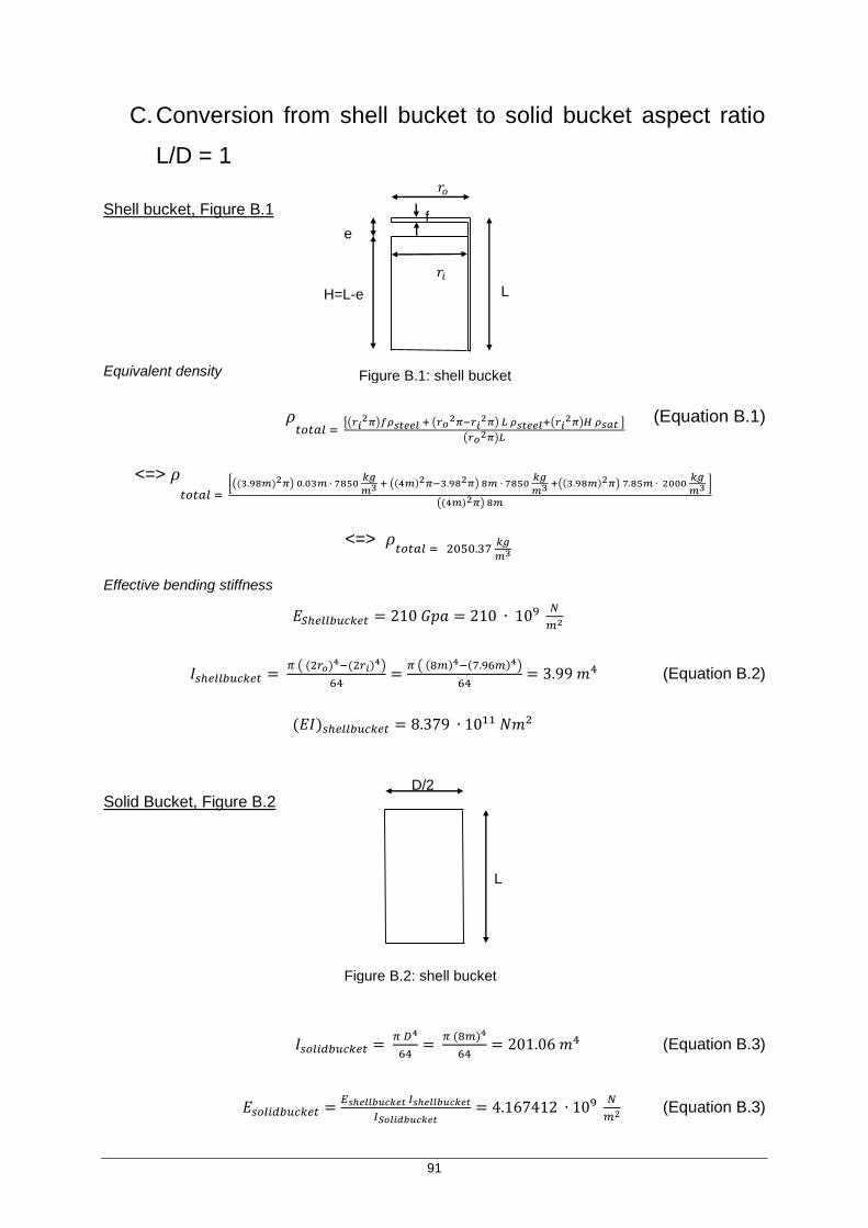
91
C. Conversion from shell bucket to solid bucket aspect ratio
L/D = 1
Shell bucket, Figure B.1
Equivalent density
𝜌𝑡𝑜𝑡𝑎𝑙 =
[(𝑟𝑖2𝜋)𝑓𝜌𝑠𝑡𝑒𝑒𝑙 + (𝑟𝑜
2𝜋−𝑟𝑖2𝜋) 𝐿 𝜌𝑠𝑡𝑒𝑒𝑙+(𝑟𝑖
2𝜋)𝐻 𝜌𝑠𝑎𝑡 ]
(𝑟𝑜2𝜋)𝐿
(Equation B.1)
<=> 𝜌𝑡𝑜𝑡𝑎𝑙 =
[((3.98𝑚)2𝜋) 0.03𝑚 ∙ 7850 𝑘𝑔
𝑚3 + ((4𝑚)2𝜋−3.982𝜋) 8𝑚 ∙ 7850 𝑘𝑔
𝑚3 +((3.98𝑚)2𝜋) 7.85𝑚 ∙ 2000 𝑘𝑔
𝑚3 ]
((4𝑚)2𝜋) 8𝑚
<=> 𝜌𝑡𝑜𝑡𝑎𝑙 = 2050.37
𝑘𝑔
𝑚3
Effective bending stiffness
𝐸𝑆ℎ𝑒𝑙𝑙𝑏𝑢𝑐𝑘𝑒𝑡 = 210 𝐺𝑝𝑎 = 210 ∙ 109 𝑁
𝑚2
𝐼𝑠ℎ𝑒𝑙𝑙𝑏𝑢𝑐𝑘𝑒𝑡 = 𝜋 ( (2𝑟𝑜)4−(2𝑟𝑖)4)
64=
𝜋 ( (8𝑚)4−(7.96𝑚)4)
64= 3.99 𝑚4 (Equation B.2)
(𝐸𝐼)𝑠ℎ𝑒𝑙𝑙𝑏𝑢𝑐𝑘𝑒𝑡 = 8.379 ∙ 1011 𝑁𝑚2
Solid Bucket, Figure B.2
𝐼𝑠𝑜𝑙𝑖𝑑𝑏𝑢𝑐𝑘𝑒𝑡 = 𝜋 𝐷4
64=
𝜋 (8𝑚)4
64= 201.06 𝑚4 (Equation B.3)
𝐸𝑠𝑜𝑙𝑖𝑑𝑏𝑢𝑐𝑘𝑒𝑡 =𝐸𝑠ℎ𝑒𝑙𝑙𝑏𝑢𝑐𝑘𝑒𝑡 𝐼𝑠ℎ𝑒𝑙𝑙𝑏𝑢𝑐𝑘𝑒𝑡
𝐼𝑆𝑜𝑙𝑖𝑑𝑏𝑢𝑐𝑘𝑒𝑡= 4.167412 ∙ 109
𝑁
𝑚2 (Equation B.3)
𝑟𝑜
𝑟
L
f e
H=L-e
𝑟𝑖
𝑟
D/2
L
Figure B.1: shell bucket
Figure B.2: shell bucket
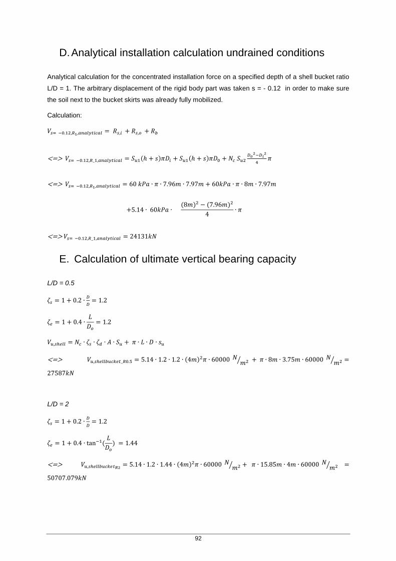
92
D. Analytical installation calculation undrained conditions
Analytical calculation for the concentrated installation force on a specified depth of a shell bucket ratio
L/D = 1. The arbitrary displacement of the rigid body part was taken s = - 0.12 in order to make sure
the soil next to the bucket skirts was already fully mobilized.
Calculation:
𝑉𝑠= −0.12,𝑅1,𝑎𝑛𝑎𝑙𝑦𝑡𝑖𝑐𝑎𝑙 = 𝑅𝑠,𝑖 + 𝑅𝑠,𝑜 + 𝑅𝑏
<=> 𝑉𝑠= −0.12,𝑅_1,𝑎𝑛𝑎𝑙𝑦𝑡𝑖𝑐𝑎𝑙 = 𝑆𝑢1(ℎ + 𝑠)𝜋𝐷𝑖 + 𝑆𝑢1(ℎ + 𝑠)𝜋𝐷0 + 𝑁𝑐 𝑆𝑢2𝐷𝑜
2−𝐷𝑖2
4𝜋
<=> 𝑉𝑠= −0.12,𝑅1,𝑎𝑛𝑎𝑙𝑦𝑡𝑖𝑐𝑎𝑙 = 60 𝑘𝑃𝑎 ∙ 𝜋 ∙ 7.96𝑚 ∙ 7.97𝑚 + 60𝑘𝑃𝑎 ∙ 𝜋 ∙ 8𝑚 ∙ 7.97𝑚
+5.14 ∙ 60𝑘𝑃𝑎 ∙ (8𝑚)2 − (7.96𝑚)2
4∙ 𝜋
<=> 𝑉𝑠= −0.12,𝑅_1,𝑎𝑛𝑎𝑙𝑦𝑡𝑖𝑐𝑎𝑙 = 24131𝑘𝑁
E. Calculation of ultimate vertical bearing capacity
L/D = 0.5
𝜁𝑠 = 1 + 0.2 ∙𝐷
𝐷= 1.2
𝜁𝑒 = 1 + 0.4 ∙𝐿
𝐷𝑜
= 1.2
𝑉𝑢,𝑠ℎ𝑒𝑙𝑙 = 𝑁𝑐 ∙ 𝜁𝑠 ∙ 𝜁𝑑 ∙ 𝐴 ∙ 𝑆𝑢 + 𝜋 ∙ 𝐿 ∙ 𝐷 ∙ 𝑠𝑢
<=> 𝑉𝑢,𝑠ℎ𝑒𝑙𝑙𝑏𝑢𝑐𝑘𝑒𝑡_𝑅0.5 = 5.14 ∙ 1.2 ∙ 1.2 ∙ (4𝑚)2𝜋 ∙ 60000 𝑁𝑚2⁄ + 𝜋 ∙ 8𝑚 ∙ 3.75𝑚 ∙ 60000 𝑁
𝑚2⁄ =
27587𝑘𝑁
L/D = 2
𝜁𝑠 = 1 + 0.2 ∙𝐷
𝐷= 1.2
𝜁𝑒 = 1 + 0.4 ∙ tan−1(𝐿
𝐷𝑜
) = 1.44
<=> 𝑉𝑢,𝑠ℎ𝑒𝑙𝑙𝑏𝑢𝑐𝑘𝑒𝑡𝑅2= 5.14 ∙ 1.2 ∙ 1.44 ∙ (4𝑚)2𝜋 ∙ 60000 𝑁
𝑚2⁄ + 𝜋 ∙ 15.85𝑚 ∙ 4𝑚 ∙ 60000 𝑁𝑚2⁄ =
50707.079𝑘𝑁

93
F. Calculation for Hult and Mo in soil with uniform strength for
different shell bucket aspect ratios
Analytical calculations were done with Equation 3-9 and values for the ultimate lateral resistance, Hult
are shown in Table 7-1 Due to the purely horizontal translation of the shell bucket, a large bending
moment (M0) will occur in the transition between foundation and support structure. An estimation of this
bending moment can be calculated with Equation 3-11.
Table 7-1: Calculation for Hult and Mo in soil with uniform strength for different shell bucket aspect
ratios
Multi-pods Monopod
Aspect ratio L/D 0.5 1 2
L (m) 4 8 16
Hult (kN) 17556 37680 71280
M0 (kNm) 35112 150720 570240