foundations of behavioral statistics

Foundations of Behavioral Statistics

Foundationsof Behavioral Statistics

An Insight-Based Approach

BRUCE THOMPSON

THE GUILFORD PRESSNew York London

© 2006 The Guilford PressA Division of Guilford Publications, Inc.72 Spring Street, New York, NY 10012www.guilford.com

All rights reserved

No part of this book may be reproduced, translated, stored in a retrievalsystem, or transmitted, in any form or by any means, electronic, mechanical,photocopying, microfilming, recording, or otherwise, without writtenpermission from the Publisher.

Printed in the United States of America

This book is printed on acid-free paper.

Last digit is print number: 9 8 7 6 5 4 3 2 1

Library of Congress Cataloging-in-Publication Data

Thompson, Bruce, 1951–Foundations of behavioral statistics : an insight-based approach /

Bruce Thompson.p. cm.

Includes bibliographical references and index.ISBN-10: 1-59385-285-1 ISBN-13: 978-1-59385-285-6 (hardcover)1. Psychometrics. 2. Psychology—Statistical methods. I. Title.

BF39.T473 2006150.1′5195—dc22

2006001101

Cover monograph, Guardians of the Morning, by Anne Moore

Preface

Young children playing in the schoolyard may fantasize about theirfuture careers, often across stunningly disparate ambitions. Forexample, very early in his schooling my younger brother strug-gled between the career choices of being either a pumpkin or an

air conditioner.But young children, or even young adults, never include statistician or

psychometrician among the options they consider. Instead, a few peoplesomewhere along the path of education discover these fields, and oftenthey are surprised by their unanticipated interest.

I first became interested in statistics and measurement as a young,first-year high school teacher taking a required master’s degree course inresearch methods. I was so exhausted from my new job that one night Ifell asleep in class.

But that class and its content eventually captivated my interest, andeven my passion, once I realized that methodology is not about math.Instead, good social science research is primarily about thinking, aboutreflection, and about judgment.

Moreover, studying social science phenomena is just plain interesting,because people are so interesting. Of course, this does not mean thatstudying people is easy. On the contrary, because people are so different

v

from each other, studying people is really quite challenging (Berliner,2002).

I hope that you, too, will find yourself captivated at least a bit by themethodological challenges inherent in studying people. In any case,through the years I have learned that students expect their professors to bepassionate about what they teach, even when the students do not fullyshare these interests.

I hope that you will sense some of my excitement in this book. I alsohope that this book, under a best-case scenario, will leave you with twofundamental reactions:

1. “This is the clearest book I have ever read.”2. “This book made me think, but also maybe even made me a better

thinker.”

The book does have several features that together I believe makeit unique, in addition to what I hope is its clarity and thought-provocativeness. First, the book emphasizes the General Linear Modelconcepts, which involve understanding how different statistical methodsare related to each other. Second, the book emphasizes effect sizes andconfidence intervals; these are old statistical ideas that are now in the fore-front of contemporary social science. Third, the book includes many con-crete hypothetical datasets, as well as the encouragement to use computersoftware (e.g., the statistical package SPSS, and the spreadsheet programExcel) to confirm and further explore statistical dynamics. For conve-nience, some datasets used in the book have been posted on the web at theURL http://www.coe.tamu.edu/~bthompson/datasets.htm. Also posted arevarious other datasets. These can be quite useful in exploring statisticaldynamics, or to develop mastery of software via practice.

This book has not been written as a sterile, formal, impenetrable trea-tise. The book teaches formulas, not as an end in themselves, but as vehi-cles to facilitate understanding of key concepts. Rote memory of legions offormulas is less relevant in an environment populated by modern hard-ware and software. Moreover, the book is written in my voice, and I speakdirectly to you. My hope is that you will find this approach engaging andstimulating.

In closing, I would be remiss if I failed to thank all the students over

vi Preface

so many years who have taught me so much about statistics, as well asclarity of thinking and articulation, among other things. Teaching is theultimate learning experience. I learn more every time I revisit each topic ina lecture or class discussion, no matter how mundane the topic or howwell traveled the road.

I appreciate the helpful suggestions from reviewers selected by thePublisher and unknown to me at the time of their reviews: Robin K.Henson, Department of Technology and Cognition, University of NorthTexas; Jeff Kromrey, Department of Educational Measurement andResearch, University of South Florida; David Morse, Department ofPsychology, Mississippi State University; Victoria Rodlin, Statistical Con-sultant (former faculty, Department of Psychology, California State Uni-versity, Fullerton); Frank Schmidt, College of Business, University of Iowa;Paul R. Swank, Department of Pediatrics, University of Texas HealthScience Center at Houston; Bruce Thyer, College of Social Work, FloridaState University; Ken Wallston, School of Nursing, Vanderbilt University;David Weakliem, Department of Sociology, University of Connecticut,Storrs. Additionally, several colleagues (Laurie Goforth, Bonnie Haecker,Oi-Man Kwok, and Janet Rice) provided insightful comments on sectionsof the draft manuscript. I have not followed this counsel in all cases, andso necessarily must remain responsible for the work in its final form.

I also thank my Publisher, C. Deborah Laughton, with whom I havenow worked for more than 10 years, for her support and encouragement.I quite vividly remember our first dinner in New Orleans in April 1994. Iwill also never forget some of our degustation dinners since, including anear “death-by-chef” experience in Manhattan. One has to love anybodywho drives a car with personalized license plates admonishing,“BE SILLY.” I am guardedly optimistic that someday she will confesswhat the “C” stands for.

BRUCE THOMPSON

Texas A&M University andBaylor College of Medicine (Houston)

Preface vii

Contents

1 Introductory Terms and Concepts 1

Definitions of Some Basic Terms 3Levels of Scale 13Some Experimental Design Considerations 24

�� Some Key Concepts 30

�� Reflection Problems 30

2 Location 31

Reasonable Expectations for Statistics 32Location Concepts 33Three Classical Location Descriptive Statistics 36Four Criteria for Evaluating Statistics 46Two Robust Location Statistics 47



3 Dispersion 53

Quality of Location Descriptive Statistics 54Important in Its Own Right 54Measures of Score Spread 57Variance 62Situation-Specific Maximum Dispersion 67Robust Dispersion Descriptive Statistics 69Standardized Score World 70



ix

4 Shape 75

Two Shape Descriptive Statistics 76Normal Distributions 86Two Additional Univariate Graphics 91



5 Bivariate Relationships 97

Pearson’s r 99Three Features of r 101Three Interpretation Contextual Factors 110Psychometrics of the Pearson r 116Spearman’s rho 118Two Other r-Equivalent Correlation Coefficients 124Bivariate Normality 128



6 Statistical Significance 133

Sampling Distributions 135Hypothesis Testing 142Properties of Sampling Distributions 150Standard Error/Sampling Error 154Test Statistics 156Statistical Precision and Power 169pCALCULATED 177



7 Practical Significance 185

Effect Sizes 187Confidence Intervals 200Confidence Intervals for Effect Sizes 207



8 Multiple Regression Analysis: Basic GLM Concepts 215

Purposes of Regression 217Simple Linear Prediction 220

x Contents

Case #1: Perfectly Uncorrelated Predictors 232Case #2: Correlated Predictors, No Suppressor Effects 234Case #3: Correlated Predictors, Suppressor Effects Present 237β Weights versus Structure Coefficients 240A Final Comment on Collinearity 244



9 A GLM Interpretation Rubric 247

Do I Have Anything? 248Where Does My Something Originate? 266Stepwise Methods 270Invoking Some Alternative Models 278



10 One-Way Analysis of Variance (ANOVA) 303

Experimentwise Type I Error 304ANOVA Terminology 309The Logic of Analysis of Variance 311Practical and Statistical Significance 317The “Homogeneity of Variance” Assumption 319Post Hoc Tests 325



11 Multiway and Other Alternative ANOVA Models 333

Multiway Models 333Factorial versus Nonfactorial Analyses 343Fixed-, Random-, and Mixed-Effects Models 345Brief Comment on ANCOVA 354



12 The General Linear Model (GLM): ANOVA via Regression 359

Planned Contrasts 360Trend/Polynomial Planned Contrasts 375

Contents xi

Repeated-Measures ANOVA via Regression 380GLM Lessons 385



13 Some Logistic Models: Model Fitting in a Logistic Context 393

Logistic Regression 394Loglinear Analysis 413



Appendix: Scores (n = 100) with Near NormalDistributions

427

References 431

Index 449

About the Author 457

xii Contents

1

Introductory Termsand Concepts

Most of us at some point have been asked to tell others theessence of who we are or to describe a friend to a third party;or friends may have described to us other people whom wehad not yet met. For example, you may have been offered the

opportunity for a blind date. Most of us develop the survival skills to ask alot of questions when these opportunities arise!

The problem is that it is difficult to summarize a person by only a fewcharacteristics. Some people may be easier to represent than others (e.g.,“She is just so nice!”). But we probably perceive most people to be multi-dimensional, and so several different characterizations may be necessaryto even begin to represent complex personalities (e.g., “He is intense, bril-liant, and incredibly funny”).

The kinds of characterizations of interest depend upon both who weare, and our purposes. We will ask somewhat different questions if we aredeciding whom to hire for a job, from whom to receive cooking advice, orwhom we should date.

Similar dynamics arise when we are trying to understand data or to

1

characterize data to others. Maybe some data can be described by a singlecharacterization (e.g., “the mean score was 102.5”). But more often thannot several different kinds of characterizations are needed (e.g., “the dataranged from 83.0 to 116.5, and the most frequent score was 99.0”).

And as in describing people, which characterizations are relevantwhen describing data depend largely upon our purposes. Sometimes themean is essential; sometimes the mean is completely irrelevant.

Finally, our personal values affect which and how many characteriza-tions may be needed to describe a potential blind date (e.g., one personmay be most concerned about the blind date’s wealth, but another may bemost interested in the candidate’s sexiness). Similarly, in statistics expertsreach different decisions about how best to understand or represent data,even when their research has the same purposes. Researcher values andinterests inherently affect how we characterize data.

In other words, statistics is not about always doing the same dataanalysis no matter what is the research purpose or situation and no matterwho is the researcher. Nor is statistics about black and white or univer-sally-right or universally-wrong analytic decisions. Instead, statistics isabout being reasonable and reflective.

Statistics is about thinking. In the words of Huberty and Morris(1988), “As in all statistical inference, subjective judgment cannot beavoided. Neither can reasonableness!” (p. 573).

The good news for mathphobic students is that statistics and researchare not really about math and computation. The bad news, however, isthat statistics and research are about thinking. And thinking can be muchmore challenging (but also much more exciting) than rote calculation orrote practice.

Statistics is about both understanding and communicating the essenceof our data. If all studies were conducted with only three or seven or ninepeople, perhaps no statistics would ever be necessary. We could simplylook at the data and understand that the intervention group receiving thenew medication did better than the control group receiving placebo sugarpills.

But when we conduct studies with dozens, or hundreds, or tens ofthousands of participants, even the most brilliant researcher cannot simplystare at the data and see all (or perhaps any) of the themes within the data.With datasets of realistic size, we require statistics to help us understandthe story underlying our data, or “to let the data speak.” Statistics were

2 FOUNDATIONS OF BEHAVIORAL STATISTICS

invented by people, for people, to help us characterize the relevant featuresof data in a given context for a given purpose.

And even if a researcher was so astoundingly brilliant as to be ablesimply to examine huge datasets and understand all the underlyingthemes, statistics would still be needed to communicate the results to oth-ers. For example, even presuming that some researcher could look at theachievement test scores of 83,000 elementary school students and under-stand their performance, most newspapers and journals would balk atreprinting all 83,000 scores to convey the results to their readers. Statis-tics, then, are also needed to facilitate the economical communication ofthe most situationally-relevant characterizations of data.

�� Definitions of Some Basic Terms

Variables versus Constants

Research is about variables and, at least sometimes, constants. A variableconsists of scores that in a given situation fall into at least two mutuallyexclusive categories. For example, if you have data on the gender of yourclassmates, as long as at least two people differ in their gender, your dataconstitute a variable.

If your class consists of 1 male and 16 females, the data constitute avariable. If the class consists of 8 males and 9 females, the data constitutea variable. If the class consists of 16 males and 1 female, the gender dataconstitute a variable.

The number of variable categories is also irrelevant in determiningwhether a variable is present, as long as there are at least two categories.For example, if your class consists of 5 males, 11 females, and 1 personwho has split XY chromosomes, you still have a variable.

Of course, it is always possible (and sometimes desirable) to collectdata consisting of a single category. A constant consists of scores that in agiven situation all fall within a single category. For example, if all the stu-dents in a class are females, the gender data in that class on this occasionconstitute a constant. Obviously, sometimes data that are constants in onesituation (Professor Cook’s class) are variables in another situation (Pro-fessor Kemp’s class).

1. Introductory Terms and Concepts 3

In some situations we purposely constrain scores on what could bevariables to be constants instead. We do so to control for possible extrane-ous influences, or for other reasons. For example, if we are conductingstudies on metabolizing huge quantities of alcohol, we may limit the studyto men because we believe that men and women metabolize alcohol differ-ently. We don’t have to worry about these differences if we limit our focusto men, and examine dynamics in women in a subsequent study, or letother researchers examine alcohol phenomena involving women. Or, wemight limit the study to only men, knowing that some female study partic-ipants might be pregnant, and we do not want to risk damaging anybabies of mothers who may not realize they are pregnant by having themdrink large quantities of alcohol during our study.

No statistics are needed either to understand or to communicate aconstant. It is easy to both understand and communicate that “all the stu-dents were females.”

But statistics are often needed to understand data collected on vari-ables, even if we collect data only on a single variable. Univariate statisticsare statistics that can be computed to characterize data on a single vari-able, either one variable at a time in a study with multiple variables, orwhen data have been collected only on a single variable.

By the way, now is as good a time as any to let you in on a secret (thatactually is widely known, and thus not really secret): The language of sta-tistics is intentionally designed to confuse the graduate students (andeveryone else). This mischievousness takes various forms.

First, some terms have different meanings in different contexts. Forexample, univariate statistics can be defined as “statistics that can be com-puted to characterize data from a single variable,” but in another context(which we will encounter momentarily) the same term has a differentmeaning.

Second, we use multiple synonymous names for the same terms. Thissecond feature of statistical terminology is not unlike naming all sevensons in a family “George,” or the Bob Newhart television show on whichone of three brothers regularly made the introduction, “This is my brotherDarrell, and this is my other brother Darrell.”

Of course, at the annual summer statistical convention (called acoven), which statistics professors regularly attend to make our languageeven more confusing, an important agreement was reached long, long ago.


It is not reasonable to confuse the graduate students on unimportantterms. Thus, we have more synonymous terms for the most importantconcepts, and consequently the importance of a concept can be intuited bycounting the number of recognized synonymous terms for the concept.

The implication is that you, unfortunately, must become facile with allthe synonymous terms for a concept. You never know which terminologyyou will encounter in published research that reflects merely the arbitrarystylistic preferences of given scholars. So you must master all the relevantsynonyms, even though the failure of statisticians to agree on uniform ter-minology is frustrating for all of us.

We may need and use statistics when we have only a single variable(e.g., to describe the spreadoutness of the scores on the midterm test or toidentify the most frequently scored score on the midterm test). But whenwe conduct research we always have at least two variables.

Research is always about the business of identifying relationships thatreplicate under stated conditions. We never conduct scholarly inquiryinvestigating only a single variable. For example, we never study onlydepression. We may study how diet seems to affect depression, or howexercise seems related to self-concept. But we never study only depression,or only self-concept.

Dependent versus Independent Variables

When we conduct research, usually there is one variable from among allthe variables in which we are most interested. This variable is called thedependent variable (or, synonymously, the “criterion,” “outcome,” or“response” variable). Clearly this is an important variable, else why wouldthis variable have so many names?

Dependent variables may be caused by or correlated with other vari-ables. A variable of the second sort is an independent variable (also calleda “predictor” variable).

Within the researcher’s theory of causation, dependent variablesalways occur after or at the same time as independent variables. Outcomescannot logically flow from subsequent events that occur after the out-come.

However, the dependent variable is the first variable selected by the


researcher. The researcher may declare, “I care about math achievement.”And then the researcher selects what is believed to be the most reasonableindependent variable. The one exception to this generalization is inapplied program evaluation, when we evaluate existing programs and thenconceptualize various possible program effects, including effects that areeither intended or unintended.

In scientific inquiry, we do not select independent variables, and thenwander around checking for all the various things that these independentvariables might or might not impact. This is not by any means meant tosay that important things can only be discovered through formal scientificmethods.

For example, Fleming discovered penicillin when some mold appar-ently drifted through an open lab window one night and landed on a petridish, thereby killing some bacteria that he was investigating. Viagra wasinitially investigated as a heart medication, but male patients beganreporting unexpected side effects. These initial discoveries were serendipi-tous, and not scientific, but nevertheless were important.

But we usually adopt as a premise the view that new discoveries willbe most likely when inquiry is more systematic. We select the outcome wecare about, and most want to control or predict, and only then do weidentify potential causes or predictors that seem most promising, givencontemporary knowledge.

Incidental Variables

Of course, in most studies many incidental variables are present, althoughnot of primary interest. Some of these data may be recorded and reportedfor descriptive purposes, to characterize the makeup of a sample (e.g., eth-nic representation or age). Other incidental variables may be of no interestwhatsoever, and may not even be recorded.

For example, a researcher may investigate as an independent variablethe effects of two methods of teaching statistics to doctoral students. Onemethod may involve rote memorization and the use of formulas; the othermethod may be insight-focused and Socratic. Final exam scores may con-stitute the dependent variable.

In any study of this sort, there would be a huge number of incidental


variables (e.g., length of right feet, soda preferences, political party affilia-tions, Zodiac signs) that occur but are of no theoretical interest whatso-ever, and therefore are usually not even recorded.

Univariate versus Multivariate Analyses

Although formal inquiry always involves at least two variables (at leastone dependent variable, and at least one independent variable), it is usualthat a given study will involve more than two variables. Because mostresearchers believe that most outcomes are multiply caused (e.g., hearthealth is a function not only of genetics, but also of diet and exercise),most studies involve several independent variables.

By the same token, most independent variables have multiple effects.For example, an effective reading intervention will impact the readingachievement scores of sixth graders, but also may well impact the self-concepts of these students. Fortunately, just as studies may involve morethan one independent variable, studies may also involve more than one de-pendent variable.

When a study involves two or more independent variables, but onlyone outcome variable, researchers use statistical analyses suitable forexploring or characterizing relationships among the variables. The class ofstatistical analyses suitable for addressing these dynamics is calledunivariate statistics, which invokes the second, alternative definition ofthis term: “methods suitable for exploring relationships between one de-pendent variable and one or more independent variables.” Univariateanalyses have names such as “analysis of variance” or “multiple regres-sion,” and are the sole focus of this book.

When a study involves two or more dependent variables, researchersmay conduct a series of univariate analyses of their data. For example, if astudy involves five dependent variables, the researcher might conduct fivemultiple regression analyses, each involving a given outcome variable inturn.

Alternatively, when a study involves two or more dependent variables,researchers may conduct a single analysis that simultaneously considers allthe variables in the dataset, and all their influences and interactions with


each other. This alternative to univariate statistics invokes multivariatestatistics.

Thompson (2000a) emphasized that “univariate and multivariateanalyses of the same data [emphasis added] can yield results that differnight-and-day [emphasis added] . . . and the multivariate picture in suchcases is the accurate portrayal” (p. 286). However, multivariate statisticsare beyond the scope of the present treatment.

Given that (a) researchers quite often conduct studies involving two ormore criterion variables, and (b) multivariate analyses provide accurateinsights into these data, why must we learn univariate statistics? There aretwo reasons. First, sometimes researchers do conduct reasonable studieswith only one dependent variable. Second, understanding univariate statis-tics is a necessary precondition for understanding multivariate statistics.Indeed, mastery of the content of this book will make learning multi-variate statistics relatively easy. Learning this content actually will beharder than learning the multivariate extensions of these concepts.

Mastery of the concepts of this book will give you the equivalentempowerment that the ruby slippers gave Dorothy in The Wizard of Oz.You will have the power to go to Kansas (or not) whenever you wish (ornot wish). Unlike the kind Witch of the North, however, I am telling youabout your empowerment at the beginning, rather than withholding thisknowledge so that the information can be revealed in a surprise ending. (Ihave always wondered why Dorothy didn’t deck the kind witch at the endof the movie, once the witch revealed to Dorothy the power she had pos-sessed all along; Dorothy might have avoided some painful and difficultsituations if the kind witch had not been so intellectually withholding.)

Symbols

When we are presenting statistical characterizations of our data, we oftenuse Roman or Greek letters to represent the characterization beingreported (e.g., M, SD, r, σ, β). This is particularly useful when we are pre-senting formulas, as in statistics textbooks. For example, we convention-ally use M (or X) as the symbol for the mean (i.e., arithmetic average) ofthe data for a given variable.

We also often use Roman letters (e.g., Y, X, A, B) to represent vari-


ables. Because independent variables tend to first occur chronologically,and dependent variables occur last, to honor this sequence we typically useletters from near the end of the alphabet to represent outcomes, and lettersfrom nearer the beginning of the alphabet to represent predictor or inde-pendent variables. For example, a researcher may declare that Y representsdegree of coronary occlusion, X1 represents amount of exercise, and X2

represents daily caloric intake. Or a researcher might investigate the effectsof gender (A) and smoking (B) on longevity (Y).

The symbols for statistical characterizations and for variables can alsobe combined. For example, once Y has been declared the symbol repre-senting the variable longevity, MY is used to represent the mean longevity.

Moderator versus Mediator Variables

In some studies we may also study the effects of a subset of independentvariables called moderator variables. In the words of Baron and Kenny(1986), “a moderator is a . . . variable that affects the direction and/orstrength of the relation between an independent or predictor variable anda dependent or criterion variable” (p. 1174).

Some variables may have causal impacts within some groups, but notothers, or may have differential impacts across various subgroups. Forexample, taking a daily low dose of aspirin reduces the risk of stroke orinfarct. But apparently about 20% of adults are “aspirin resistant,” andfor these patients the independent variable, aspirin dosage, has little or noeffect on the outcome, infarct incidence.

As another example, Zeidner (1987) investigated the power of a scho-lastic aptitude test to predict future grade point averages. He found thatpredictive power varied across various age groups. In this example, GPAwas the dependent variable, aptitude was the independent variable, andage was the moderator variable.

Moderator effects can be challenging to interpret. Simpson’s Paradox(Simpson, 1951) emphasizes that relationships between two variables maynot only disappear when a moderator is considered, but also may evenreverse direction! Consider the following hypothetical study in which anew medication, Thompson’s Elixir, is developed to treat patients with


very serious coronary heart disease. The results of a randomized clinicaltrial (RCT), a 5-year drug efficacy study, are presented below:

Outcome Control Treatment

Live 110 150Die 121 123% survive 47.62% 54.95%

The initial interpretation of the results suggests that the new medica-tion improves 5-year survival, although the elixir is clearly not a panaceafor these very ill patients. However, mindful of recent real research sug-gesting that a daily aspirin may not be as helpful for women as for men inpreventing heart attacks, perhaps some inquisitive women decide to lookfor gender differences in these effects. They might discover that for womenonly these are the results:


Live 58 31Die 99 58% survive 36.94% 34.83%

Apparently, for women considered alone, the elixir appears less effectivethan the placebo.

Initially, men might rejoice at this result, having deduced from the twosets of results (i.e., combined and women only) that Thompson’s Elixirmust work for them. However, their joy is short-lived once they isolatetheir results:


Live 52 119Die 22 65% survive 70.27% 64.67%

In short, for both women and men separately, the new treatment is lesseffective than a placebo treatment, even though for both genders com-bined the elixir appears to have some benefits.


The paradox that any relationship between variables may be changed,or even reversed, by introducing a moderator makes clear how vital is thedecision of what variables will be considered in an analysis. In the presentexample, we might deem the results for genders combined to be the rele-vant analysis, and consider using the elixir, notwithstanding the paradoxi-cal differences within the categories of the moderator variable.

In addition to investigating moderator effects, we also sometimesstudy the effects of mediator variables. Whereas moderator variablesinform judgment about when or for whom effects or relationships operate,mediator variables may help us understand how or why effects or relation-ships occur.

Independent variables may have some combination of both direct andindirect effects. Mediator variables are used to explore and quantify theindirect versus the direct effects of an independent variable upon a depen-dent variable.

For example, for the largest 50 cities in the United States, there is ahuge relationship between the number of churches and the number ofannual murders. However, if we take into account the mediating influenceof city size, there is virtually no relationship between numbers of churchesand murders. That is, virtually all the “effects” of number of churches onmurders is indirect, via the mediation of city size.

Any observed relationship between churches and murders is spurious.Taking into account city size, we see that churches do not apparentlyexplain or predict murders. Nor do more or fewer murders apparentlylead to building more or fewer churches!

As a second example, consider the relationship between fathers’ edu-cation and oldest child’s subsequent education, mediated by fathers’ socio-economic status. Fathers’ education may have a mixture of both direct andindirect effects on the educational attainment of children. More educatedfathers may teach children to value attainment, and may also teach theirchildren educational content.

But fathers’ education additionally impacts fathers’ socioeconomicstatus. And fathers’ socioeconomic status may, in turn, have its ownimpacts on the educational attainment of children, because social classmay influence children’s aspirations, expectations, and the knowledgeexchanged by peers in classrooms and other settings.


Populations versus Samples

Whenever we conduct quantitative or mixed-methods (Tashakkori &Teddlie, 2002) research, there is the group of people (or lab rats or mon-keys) about which we wish to generalize, and the group from which wehave data. The group to which we wish to generalize is called the popula-tion. If we have data only from a subset of the population, our dataset iscalled a sample.

If I collect data in a teaching experiment from 20 doctoral students ina given time period, and these are the only students about whom I care,then this group constitutes a population. But if I give you my data, andyou wish to use these data to generalize to other graduate students, or forthese students to other points in time, then for you these same data consti-tute a sample.

The distinction between a population and a sample is solely in the eyesof the beholder. Two researchers looking at the same data may make dif-ferent decisions about the generalization of interest.

The distinction is made on the basis of research purpose, and not onthe basis of data representativeness. Indeed, there is an old cliché thatmuch social science research involves unrepresentative samples and is con-ducted “on rats and college sophomores.” Regardless of the mechanism ofsampling (e.g., a sample of local convenience), if the researcher is general-izing to a larger population, the data constitute a sample, even though thesample may not be very good, or representative.

In practice, researchers almost always treat their data as constituting asample. Researchers seem to be quite ambitious! For example, in conduct-ing an intervention experiment with 10 first graders who are being taughtto read, even if the sample consists only of children who are familyacquaintances, scholars seemingly prefer to generalize their findings to allfirst graders, everywhere, for all time.

Thus, when we take courses about quantitative ways to characterizedata, we tell people we are taking a “statistics” course rather than a“parameters” class or a “statistics/parameters” class. In actuality, it mightbe more accurate to say that we are taking a course about “statistics/parameters.”

The judgment as to whether data constitute a population or a sampleis not semantic nit-picking. For some characterizations of data, formulas


for a given characterization differ, depending on whether or not the dataare deemed a sample or a population. So two researchers who are comput-ing the same result even for the same data may obtain different numericalanswers if they reach different judgments about the population of interest.

Characterizations of data computed for populations are termedparameters. Parameters are always represented by Greek letters. Forexample, if we have data for 12 doctoral students at a given time on thevariable X, and we only care about these students at this single point intime, the data constitute a population. The arithmetic average, or mean, ofthese 12 scores would be represented by the Greek letter µX.

Characterizations of sample data are called statistics. For example, ifwe have the same data for 12 doctoral students at a given point in time,and we believe we can generalize their results to other doctoral students,and we desire to make this generalization, our data instead constitute asample. The arithmetic average, or mean, of these 12 scores would be rep-resented by a Roman letter, such as MX or X .

As another mnemonic device to help distinguish populations fromsamples, we will also use different symbols to represent the number ofscores in populations versus samples. We will use N to quantify the num-ber of scores in a population, and n to quantify the number of scores insamples.

�� Levels of Scale

Quantitative data analysis typically involves information represented inthe form of numbers (e.g., the dataset for a sample of n = 3 people: 1, 2,3). However, different sets of the same three numbers (i.e., 1, 2, and 3)may contain different amounts of information.

Furthermore, when we characterize different aspects of data, eachcharacterization presumes that the numbers contain at least a certainamount of information. If we perform a calculation that requires moreinformation than is present in our data, the resulting characterization willbe meaningless or erroneous.

So the judgment about the amount of information each dataset con-tains is fundamentally important to the selection of appropriate formulas


for data characterizations. And for every way of characterizing data, wemust learn the minimum information that must be present to compute agiven statistic or parameter.

Four Levels of Scale

Quantitative researchers characterize the amount of information con-tained in a given variable by using levels of scale conceptualized byS. Stevens (1946, 1951, 1968) and others. The four levels of scale are:(a) nominal/categorical, (b) ordinal/ranked, (c) interval/continuous, and(d) ratio. More detail on levels of scale is provided by Nunnally (1978,Ch. 1), Guilford (1954, Ch. 1), and Kirk (1972, Ch. 2).

The levels of scale constitute a hierarchy. Data at a given level of scalecontain all the information unique to the given level plus all the informa-tion present at lower levels of scale.

For each level of scale, there are specific constraints on what numberswe may use to represent the information contained in a variable. At thesame time, even given these constraints, infinitely many reasonable choicesalways still exist for communicating a given variable’s information.

Knowing the numbers used to represent scores on a given variabletells you nothing about the level of scale of the data. It is the informationpresent in the data, as determined by the mechanisms of measurement,that determines scaling. And, as might be expected by now, because theseconcepts are important, there are synonymous names for several of thelevels of scale.

Nominal or categorical data represent only that (a) the categories con-stituting a given variable are mutually exclusive, and (b) every person scor-ing within a given category is identical with respect to the particularvariable being measured. Human gender of a particular class of students isa variable iff (if and only if) at least two students in this class have a differ-ent gender. We usually take human gender in many groupings to bedichotomous (i.e., a two-category variable). Worms are an entirely differ-ent story. For people, the commonly-recognized categories are “male” and“female.” Because very, very few people are hermaphrodites, presumablythe categories in our given class of students are mutually exclusive.

We also consider every person in a given category to be exactly identical


with respect to the variable, gender. All males are exactly equally male, andall females are exactly equally female. This does not mean that all the males,or all the females, have the same physical measurements, sex appeal, money,intelligence, or anything else. But every person in a given category of a givenvariable is considered exactly the same as regards that variable.

Consider the data for the following four students on the variable gen-der (X):

Name X

Steve MPatty FJudy FSheri F

In quantitative research we typically represent information using numbers,rather than letters or other symbols.

In converting these data to numbers, we must honor the two pieces ofinformation present on the variable. Thus, we cannot assign the samenumber (e.g., 0) to all four students, or we would misrepresent the realitythat the categories are mutually exclusive. Nor could we legitimately givePatty one number, and Judy and Sheri a different number, or we wouldmisrepresent the reality that Patty, Sheri, and Judy are all consideredequally female.

Notwithstanding these constraints, which are absolute, there remaininfinitely many plausible choices. We could assign Steve “1,” and theremaining students “2.” Or we could assign Steve “1,” and everyone else a“0.” Alternatively, we could assign Steve “999,999,999,” and the remain-ing students each “–5.87.” Or we could assign Steve “6.7,” and Patty,Judy, and Sheri each “–100,000.”

Let us assume that a researcher selected the first scoring strategy (i.e.,“M” = “1”; “F” = “2”). This is perfectly acceptable. But when analyzingour data, it is essential to remember what information is present in thedata, and what information is not. Given the nominal level of scale of ourdata, we know only that we have two mutually-exclusive categories, andthat everyone in a given category is identical with respect to gender. Our


scoring does not mean that two males equal one female, or that concern-ing gender a male is half a female!

Given the information present in nominal data, the only mathematicaloperation permissible with such variables is counting. For example, wecan say that female is the category with the most people, or that there arethree times as many females as males.

Ordinal or ranked data contain the two features of nominal data butalso warrant that (c) score categories have a meaningful order. Let’s saywe have data for our sample of n = 4 people on a second variable, militaryrank (Y):

Name Y

Steve GeneralPatty CaptainJudy PrivateSheri Private

When translating this information into numerical scores, there areagain both constraints, and infinitely many plausible alternatives. We canassign scores of 1, 2, 3, and 3, respectively. Or we can assign scores of 9, 8,1, and 1. Or we can assign scores of –0.5, –2.7, –1,000,000,000, and–1,000,000,000.

We may not assign scores of 4, 4, 2, and 1, or we misrepresent charac-teristic #1. We may not assign scores 1, 2, 3, and 4, or we dishonor char-acteristic #2. We may not assign scores of 1, 3, 2, and 2, or wemisrepresent characteristic #3.

If we assign the scores, 3, 2, 0.5, and 0.5, respectively, we have hon-ored all the necessary considerations for these data. But this does notmean that Steve has exactly the same military authority as Patty, Judy, andSheri when they act in concert, even though 2 plus 0.5 plus 0.5 does math-ematically sum to 3.

With ordinal data, as with data at all the levels of scale, we can alwaysperform counting operations. So, for these data we can say that Private isthe most populous category on this variable, or that 50% of the samplehad the rank of Private.

But now we can also perform mathematical operations that require


ordering the scores. For example, we can now make comparative state-ments, such as Patty has less authority than Steve. But we cannot quantifyhow much less authority Patty has versus Steve.

Interval or continuous data contain the previous three informationfeatures, but also (d) quantify how far scores are from each other using a“ruler,” or measurement, on which the units have exactly the same dis-tances. Consider the following scores for variable X, a measure of self-concept on which scores of zero are impossible because sentient beings arepresumed to have some self-image:

Name X

Steve 183Patty 197Judy 155Sheri 141

These data create a four-category intervally-scaled variable. Note thatit is the interval quality of the measuring “ruler,” and not the scores them-selves, that must be equally spaced. Every additional point represents anequal amount of change in self-concept.

We can again represent these scores in infinitely many ways, as long aswe do not misrepresent the information. For example, we could withoutdistortion convert the scores by dividing each score by 10. Doing so wouldnot dishonor the order of the scores, or the relative distances betweenscores. If one person had a score twice as large as another person, any rea-sonable reexpression of the scores would honor these (and all other rele-vant) facts, and be equally plausible. Indeed, any preference for one versusanother of these reasonable representations would be completely a matterof personal stylistic preference, and not matter otherwise.

Finally, with interval data we can perform mathematical operations ofaddition and the reciprocal operation of subtraction, as well as multiplica-tion and the reciprocal operation of division by constants, such as thesample size. It makes no sense to add scores measured with a “ruler” onwhich every interval is a different distance. But with interval scores theseoperations are sensible.

We can now quantify the distances of scores from each other. For


example, we can say that the distance between the scores of Patty andSteve is the same as the distance between the scores of Judy and Sheri.

Ratio data contain the prior four information features, but also (e)include the potential score of a meaningful zero. A zero is said to be mean-ingful if the score of zero means the complete absence of the variable beingmeasured. For example, if your net financial worth is $0, this means thatyou have exactly no money, which is both meaningful (in the sense of rep-resenting the exact absence of any money) and possible.

For many social science variables, a meaningful zero is not sensible.For example, it is impossible to imagine that a living person to whom wecould administer an IQ test would have an IQ score of exactly zero (i.e., acomplete absence of intelligence).

Scaling as a Judgment

Life is not always about definitively right or wrong choices, and neither isstatistics. For many physical measurements, such as height in centimetersor weight in pounds, clearly data are being collected at the interval level ofscale.

But most constructs in the social sciences are abstract (e.g., self-concept, intelligence, reading ability) and are not definitively measured ata given level of scale. For example, are IQ data intervally-scaled? Is the 10-point difference between Bill with an IQ or 60 and Jim with an IQ of 70exactly the same as the difference between Carla with an IQ of 150 andColleen with an IQ of 160?

Probably all methodologists would agree that measurements of thissort are at least ordinally-scaled. Furthermore, many statisticians wouldtreat such data as interval because they judge the data to truly approxi-mate intervally-scaled data. Other methodologists are statistically conser-vative, treat such data as ordinal, and only perform analyses on the datathat require only ordinal scale. You can discern the two camps at profes-sional meetings, because the latter always wear business attire and the for-mer wear blue jeans.

You might feel more comfortable about these judgments if you recog-nize that even physical measurements do not really yield perfectly interval


data. All measurements, even physical measurements, yield scores withsome measurement error, or unreliability (see Thompson, 2003). Forexample, even the official clock of the United States, which measures timeby measuring atomic particle decay, loses 1 second every 400 years. So, ifwe consider measurement reliability, no “rulers” have intervals that areperfectly, exactly equal.

Transforming Scale of Measurement

Some variables can inherently be measured only at the nominal level ofscale. For example, gender, or religious preference, or ethnic background,can only be measured categorically.

At the other extreme, some variables can be measured at any level ofscale, depending on how the researcher collects or records the scores. Con-sider the following measures of how much money these four people werecarrying at a given point in time:

Name X1 X2 X3

Steve $379 1 RichPatty $9 4 PoorJudy $78 3 PoorSheri $264 2 Rich

Given these three sets of scores, all measuring the variable wealth, X1

is certainly at least intervally-scaled, because the “ruler” measuring finan-cial worth at a given point in time in dollars measures in equal intervals.The financial value (though perhaps not the personal differential value) ofa change in any $1 is constant throughout the scale.

The variable X2 is ordinally-scaled. We have discarded informationabout the distances of datapoints from each other. We can still say that notwo people have the same wealth (i.e., are in the same category), and wecan still order the people. But with access only to the X2 data, we can nolonger make determinations about how far apart these individuals are intheir wealth.

The variable X3 is nominally-scaled. Although the categories are still


ordered, we can no longer order the individual people. We have either col-lected relatively limited information, or have chosen to discard consider-able information about wealth.

In general, collecting data at the highest possible scale is desirable. Forexample, if the researcher collects intervally-scaled data, the data canalways be converted later to a lower level of scale. Conversely, once dataare collected at a lower scale level, the only way to recover a higher levelof scale is to recollect the data.

Because statistics require specific levels of scale to properly conducttheir required mathematical operations, some statistics cannot be com-puted for data at some scale levels. Also, more analytic options exist fordata collected at higher scale levels.

However, in statistics there are exceptions to most general rules.When we are collecting information that is particularly sensitive, peoplemay be more likely to respond if data are collected at lower levels of scale.For example, we can ask people how many times they have sex in amonth, or how frequently they go to church in a year, or how muchmoney they made last year. These data would be intervally-scaled.

But people may be more likely to respond to such questions if weinstead presented a few categories (e.g., 0–2 times/month, 3–8 times/month, more than 8 times/month) from which respondents select theiranswers. This measurement strategy collects less information, and thus isless personal. Research always involves many tradeoffs of the good versusbad things that occur when we make different research decisions. Never-theless, the conscious decision to collect data at lower scale levels shouldbe based on a reflective analysis that you can still do whatever analysesyou need to do to address the research questions that are important toyou.

Normative versus Ipsative Measurement

Cattell (1944) presented a related measurement paradigm that distin-guishes between normative and ipsative measurements. Normative mea-surement collects data in such a way that responses to one item do notmechanically constrain responses to the remaining items.


Here are two items from a survey measuring food preferences:

1. Which one of the following foods do you most prefer?

A. monkfish B. filet mignon with bernaiseC. mushroom risotto D. crème brûlée

2. Which one of the following wines do you most prefer?

A. sauvignon blanc B. cabernet sauvignonC. pinot noir D. riesling

These items yield normative scores.The response to one item may logically constrain responses to other

items. For example, people who love beef with bernaise sauce may havesome tendency to prefer cabernet sauvignon. But responses to the firstitem do not physically constrain the choice made on the second item. Peo-ple can declare that their favorite food is monkfish, and that their favoritewine is riesling. Indeed, some people may actually like that pairing.

Ipsative measurement collects data such that responses to a given itemmechanically constrain choices on other items. Items of this sort haveforced-choice features, such as requirements to rank-order choices or toallocate a fixed number of points across a set of items.

The following item, with one respondent’s choices shown, yieldsipsative data:

1. Please allocate exactly 100 points to show how much you like eachof the following types of wine by awarding more points to winesyou most prefer.

A. sauvignon blanc 10B. chardonnay 15C. pinot noir 20D. merlot 10E. cabernet sauvignon 45F. malbec 0G. riesling 0TOTAL 100


This individual clearly likes cabernet.We can at least make reasonable intraindividual comparisons with

ipsative data. For example, we can argue that this person likes cabernetthree times as much as chardonnay.

These data are ipsative, because the decision to allocate a given num-ber of points to one choice necessarily constrains allocations for all otheroptions. And we have no information about whether this individualdespises wine, thinks wine is nice sometimes, or adores wine. This makesit difficult to use ipsative data to make meaningful interindividual compar-isons of results across individuals, if that is our purpose (L. Hicks, 1970).

Related data could be collected normatively, as illustrated in theseresults, which measure the actual spending decisions of two hypotheticalindividuals:

2. Please report how many dollars you would like to spend per monthon each of the following types of wine, if your income was not aconsideration.

Bruce Julie

A. sauvignon blanc $90 $0B. chardonnay $295 $125C. pinot noir $360 $0D. merlot $110 $35E. cabernet sauvignon $895 $45F. malbec $0 $0G. riesling $0 $0TOTAL $1,750 $205

These are normative and not ipsative data, because responses regardingone wine do not in any mechanical way constrain responses for theremaining wines.

Likert (1932) scales are often used to collect normative data aboutattitudes or beliefs. Likert scales present response formats with numericalscales in which some or all of the numerical values are anchored to wordsor phrases. The numerical value and word pairing might be: 1, StronglyAgree; 2, Agree; 3, Neutral; 4, Disagree; 5, Strongly Disagree. If the


researcher judges the psychological distances between these alternatives tobe equal, then the data collected are arguably intervally-scaled.

At first impression, it may seem that normative data should be pre-ferred over ipsative data. Normative data are usually intervally-scaled, andit may seem undesirable to constrain responses when collecting data.

Ipsative data collection tends to make responding more complex,because specific response rules must be followed exactly. Respondentsmay resent restrictions that have no obvious basis. Also, ipsative responseformats as a statistical artifact yield dependencies among item responses(Kerlinger, 1986, p. 463). That is, because responses to one item (e.g., ahigh allocation of points to an item) constrain responses to other items,the relationships between item responses tend to be inverse (i.e., high rat-ings on one item necessarily yield lower ratings on other items).

However, sometimes ipsative data collection is necessary. For exam-ple, in an investigation of phenomena involving variables that are allhighly treasured, normative data collection might result in every respon-dent’s rating every choice at the extremes of the response format. Ifrespondents were asked to rate the importance of health, economic suffi-ciency, attractiveness, and honor on 1-to-5 scales, it would not be unrea-sonable for everyone to rate all four items “5.”

In such situations, reasonable variability in scores can only beachieved by using ipsative measurement. Furthermore, in some cases itmight be argued that ipsative measurement is most ecologically-valid (i.e.,best honors the way in which people really function in everyday life). Forexample, people may cherish a great many outcomes (e.g., health, eco-nomic sufficiency). But given time and other resource constraints, we can-not pursue every possible thing about which we care.

In this example, ipsative measurement not only might be necessary toproduce score variability, but also may best honor the ecological reality.At least, that seems to be the thinking underlying Rokeach’s (1973) devel-opment of his Values Survey, which requires respondents to rank-orderthe different human values he lists, with no ties.

Ipsative measurement is used on a variety of psychological measures.For example, ipsative measurement is used on some tests intended to mea-sure psychopathology. Items on such measures may ask unusual questionsthat focus on atypical thought or preference patterns. The items may pose


questions virtually of the ilk, “Would you most rather be (a) a pumpkin,(b) an air conditioner, or (c) a fork?”

�� Some Experimental Design Considerations

Designs

Experiments are studies in which at least one intervention group receives atreatment, and at least one control group receives the usual treatment(e.g., conventional reading instruction) or no treatment (e.g., placebosugar pills). In true experiments, the mechanism for assigning participantsto groups is random assignment. Random assignment has the desirablefeature that groups will be equivalent at the start of the experiment on allvariables, even those the researcher does not realize are actually impor-tant, iff the sample size is sufficiently large that the law of large numberscan function. The mechanisms of random assignment simply do not workwell when sample size is very small.

Only experimental designs allow us to make definitive statementsabout causality, although other research designs may suggest the possibili-ties of causal effects (see Odom, Brantlinger, Gersten, Horner, & Thomp-son, 2005; Thompson, Diamond, McWilliam, Snyder, & Snyder, 2005).Recent movements to emphasize evidence-based practice in medicine(Sackett, Straus, Richardson, Rosenberg, & Haynes, 2000), psychology(Chambless, 1998), and education (cf. Mosteller & Boruch, 2002;Shavelson & Towne, 2002) have brought an increased interest in experi-mental design.

Classically, designs were portrayed by an array of symbols presentedon an implicit timeline moving from earlier on the left to later on the right(D. T. Campbell, 1957; Campbell & Stanley, 1963). “R” indicates ran-dom assignment to groups, “O” indicates measurement (e.g., a pretest),and “X” indicates intervention. For example, a two-group true experi-ment with no pretesting might involve

R X OR O


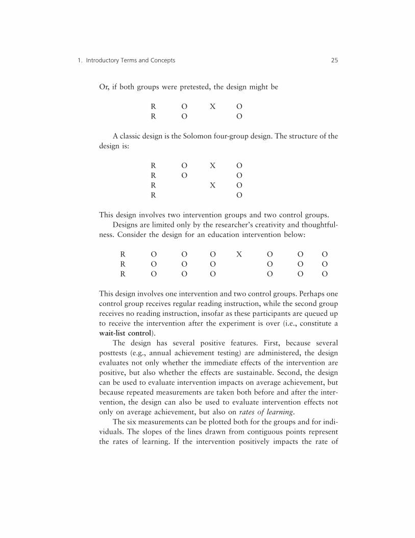
Or, if both groups were pretested, the design might be

R O X OR O O

A classic design is the Solomon four-group design. The structure of thedesign is:

R O X OR O OR X OR O

This design involves two intervention groups and two control groups.Designs are limited only by the researcher’s creativity and thoughtful-

ness. Consider the design for an education intervention below:

R O O O X O O OR O O O O O OR O O O O O O

This design involves one intervention and two control groups. Perhaps onecontrol group receives regular reading instruction, while the second groupreceives no reading instruction, insofar as these participants are queued upto receive the intervention after the experiment is over (i.e., constitute await-list control).

The design has several positive features. First, because severalposttests (e.g., annual achievement testing) are administered, the designevaluates not only whether the immediate effects of the intervention arepositive, but also whether the effects are sustainable. Second, the designcan be used to evaluate intervention impacts on average achievement, butbecause repeated measurements are taken both before and after the inter-vention, the design can also be used to evaluate intervention effects notonly on average achievement, but also on rates of learning.

The six measurements can be plotted both for the groups and for indi-viduals. The slopes of the lines drawn from contiguous points representthe rates of learning. If the intervention positively impacts the rate of


learning, the lines connecting the plotted scores will be steeper after theintervention than before the intervention. Impacting rates of learning mayhave sustained effects even more important than immediate impacts,because changing how fast people learn may have more dramatic cumula-tive consequences over time than do the immediate impacts on learning.Latent growth curve modeling (Duncan & Duncan, 1995; Duncan,Duncan, Strycker, Li, & Anthony, 1999) evaluates these various dynam-ics, although this analysis is beyond the scope of the present, introductorytext. Nevertheless, we can intuit the potential richness of data yielded bysuch designs.

Historically, designs were evaluated in terms of the ability to addresstwo sorts of design validity issues (Campbell & Stanley, 1963). Note thatdesign validity should not be confused with measurement validity (seeThompson, 2003, Ch. 1, for further discussion of measurement issues).The similarity of wording for these two unrelated concepts is merelyanother effort to invoke confusing language in statistics.

Internal Design Validity

Internal design validity addresses concerns about whether we can be cer-tain that the intervention caused the observed effects. Without internaldesign validity, study results are simply uninterpretable. Campbell andStanley (1963) listed threats to internal design validity, of which seven areconsidered here.

Selection threats to design validity occur if there are biases in assign-ing participants to groups. For example, in the following design,

O X OO O

if smarter students are disproportionately assigned to treatment, groupselection dynamics are confounded with intervention effects. Even if westatistically adjust for initial group differences, by computing and compar-ing gain scores (∆Xi = posttesti – pretesti), we will not have removed therate of learning (i.e., aptitude) differences across the groups, and the


results will remain confounded. Obviously, this is why we prefer randomassignment to groups.

Experimental mortality involves differential loss of participants fromgroups during the intervention. For example, if the intervention groupshowed posttest improvement, but 35% of the intervention group with-drew from the study, while only 5% of the control group dropped, theresults are confounded by the presence of potentially selectively missingdata.

History threats to internal design validity occur when unplannedevents that are not part of the design occur during the intervention. Forexample, if one school is the intervention site, and another school is thecontrol school, during the intervention school year an intervention schoolteacher might win hundreds of millions of dollars in a lottery, and beginshowering the school with new computers, and even books. These effectsmay confound the intervention effects such that we are not certain whatimpacts are attributable to the designed intervention.

Maturation effects involve developmental dynamics that occur purelyas a function of the passage of time (e.g., puberty, fatigue). For example, ifthe control group is a first-period high school class, and the interventiongroup is a last-period class, the differential impacts of fatigue and hungermay be confounded with intervention effects.

Testing involves the impacts of taking a pretest on the posttest scores.A pretest (e.g., a first-grade spelling test) may focus participants on tar-geted words. These effects might become confounded with interventioneffects, for example, if the design was

R O X OR O

Instrumentation may compromise result interpretation if differentmeasures (e.g., Forms X and Y of a standardized test) are used in differentgroups, or over time. For example, instrumentation effects might compro-mise this design:

R OX X OX

R OY OY


Statistical regression occurs when extreme scores exhibit the statisticalphenomenon called regression toward the mean. The phenomenon refers tothe fact that extreme scores tend to move toward the group mean over time.

Sir Francis Galton, British genius and polymath, first described thisstatistical phenomenon (Galton, 1886). At the Great Exhibition, Galtonmeasured the heights of families at the event. He observed that extremelytall or short parents tended to have adult children whose heights moreclosely approximated typical height. Clearly, the phenomenon is purelystatistical, and not some function of the exercise of will or judgment dur-ing procreation.

The phenomenon can compromise designs, for example, when partici-pants with extreme scores are assigned to groups. Thus, in a one-groupdesign, if people with very high blood pressure on pretest are assigned totreatment, in the long run their scores will tend toward the mean evenwithout treatment. The effects of medication and the statistical regressioneffect will be confounded, and we will be unable to ascertain with confi-dence what are the intervention effects.

External Design Validity

External design validity involves the question of “to what populations,settings, treatment variables, and measurement variables can this effect begeneralized?” (Campbell & Stanley, 1963, p. 175). Here, three threats willbe considered.

Reactive measurement effects occur if pretesting affects sensitivity tothe intervention. For example, a vocabulary pretest might impact theeffects of a vocabulary intervention, such that the intervention effectsmight not exactly generalize to future nonexperimental situations in whichthe intervention is conducted without pretesting.

In the 1920s, the German physicist Werner Heisenberg proposed hisUncertainty Principle, which essentially says that the more precisely theposition of atomic particles is determined, the less precisely the momen-tum of the particles can be simultaneously known. A related but more gen-eral measurement paradox says that “observing a thing changes thething.” If we don’t measure, we do not know what happens. But whathappens in the absence of our measurements might be different than whenwe measure. However, in some cases reactive measurement might be


avoided by using unobtrusive measures (Webb, Campbell, Schwartz, &Seechrest, 1966).

Hawthorne effects occur when participants in the intervention groupalter their behavior because they are aware that they are receiving specialattention. The name of the effect originates from a 5-year study conducted atthe Hawthorne Plant of the Western Electric Company in Cicero, Illinois,during the Great Depression. The researchers found that when working con-ditions were improved in the intervention group, productivity improved.However, even when less favorable conditions were imposed, productivityalso improved. The participants were apparently responding to the general-ized notion of public specialized treatment, as opposed to the interventionitself. Therefore, such intervention effects might not generalize once theintervention was applied to everyone, or at least was widely available,because the novelty of the treatment would no longer be a factor.

John Henry effects occur when participants in the control groupbehave differently because they know that they are in the control condi-tion. The effect is named after the legendary John Henry, The SteelDriving Man, who fought harder than he presumably would have becausehe knew he was in a contest and his performance was being evaluated. Inthe legend, John Henry was an African American of incredible strengthwho drove railroad spikes when track was being laid. When a steam-driven spike drill was being introduced, John Henry competed in a racewith the drill to determine whether he or the drill could drive more spikes.The race was close, and John Henry died at its end.

A double-blind design is one way to avoid Hawthorne and JohnHenry effects. In this design, the participants do not know whether theyare receiving the intervention or a placebo treatment (e.g., sugar pills), andthe treatment administrators (e.g., nurses) do not know what treatmentthey are providing. Of course, double-blind studies are feasible in medi-cine, but may not be possible in education or psychology in cases wherethe nature of the intervention simply cannot be obscured.

Design Wisdom

Here is one of the most important things I can tell you about doingresearch. When selecting variables and designing research, before you col-lect any data whatsoever, first “List [all] possible experimental findings


[i.e., results] along with the conclusions you would draw and the actionsyou would take if this or another [any/every other] result should prove tobe the case” (Good & Hardin, 2003, p. 4). This exercise forces early rec-ognition of fatal design flaws before it is too late to correct problems.

Some Key Concepts

Statistics are computed so that we can understand and communicatethe dynamics within data. Statistics are selected given the researcher’spurpose. Usually several statistics will be needed to characterize rele-vant data features within a given study. Both subjective judgment andreasonableness must be exercised when selecting statistics.

Statistics may be used to characterize data involving only a singlevariable. But science is about the business of identifying relationshipsthat occur under stated conditions, and so scientific studies inherentlyinvolve at least one dependent variable and at least one independentvariable.

The selection of ways to characterize data is also governed by adecision about whether the data constitute a sample or a population.And the levels of scale of variables impact which statistics are and arenot reasonable in a given research situation.

Only true experiments, in which treatment conditions are ran-domly assigned, can definitively address questions about causality. Toyield definitive conclusions, studies must be organized to mitigatethreats to internal and external design validity.

�� Reflection Problems ��

1. Name a nominally-scaled, an ordinally-scaled, and an intervally-scaled vari-

able, with each of the three variables involving four categories. Then

name five equally-reasonable ways to assign numbers to the categories of

each of the three variables (i.e., scoring rubrics).

2. Think of a situation, not described in this book, in which ipsative measure-

ment might be preferred over normative measurement.

3. Identify a dependent variable of particular interest to you. Then select the

two independent variables that you consider the best possible predictors of

this outcome. In a study using these three variables, would you hold any-

thing constant? What moderator variable might be of greatest interest?


2

Location

Descriptive statistics quantitatively characterize the features ofdata. Although “statistics” are always about sample data,“descriptive statistics” are about either sample or populationdata. (You have already been duly forewarned about the confus-

ing language of statistics.)Four primary aspects of data can be quantified: (a) location or central

tendency, (b) dispersion or “spreadoutness,” (c) shape, and (d) relation-ship. The first three classes are called univariate statistics, in the sense ofthis term meaning that these descriptive statistics can be computed even ifyou have data on only one variable. The fourth category of descriptive sta-tistics requires at least two variables. In the simplest case, when there areonly two variables (e.g., X and Y), or there are more than two variablesbut the variables are considered only in their various pairwise combina-tions (e.g., A and B, A and C, B and C, and never all A, B, and C simulta-neously), relationship statistics encompass bivariate statistics.

The statistics computed across these four classes are independent. Thismeans, for example, that knowing the central tendency of the data tells

31

you nothing about the numerical quantification of the dispersion of thedata, or that knowing the shape of the data tells you nothing about thenumerical quantification of the location of the data.

The independence of the four categories is only logical. If any two ofthe characterizations performed the same function, there would be fewerthan four categories. Even the most wild-eyed statisticians can only go sofar in trying to be confusing!

�� Reasonable Expectations for Statistics

Formulas for descriptive statistics were not transmitted on stone tabletsgiven to Moses, nor otherwise divinely authored. Instead, different humanpeople developed various formulas as ways to characterize quantitativedata.

Sometimes people are noble, honorable, and insightful. But sometimespeople are also lazy, sloppy, or simply wrong. Because these formulaswere created by fallible people, the prudent scholar does not take theseequations as givens, and instead evaluates whether the formulas seem tobe reasonable.

Thoughtful, critical, and responsible judgment requires initially for-mulating expectations about what might be deemed reasonable for agiven way of characterizing data. These different expectations apply toall the entries in a given class of descriptive statistics. If the descriptivestatistics are indeed reasonable, they will behave such that they alwaysmeet these expectations. Otherwise, the characterizations yielded bythese formulas are erroneous, and should be discarded in favor of cor-rect formulas.

There are advantages from understanding statistics (our focus), ratherthan merely memorizing unexplained formulas. Only when we fullyunderstand the underlying logics of the formulas, as well as which datafeatures do and do not affect results, do we really understand our charac-terizations of data (and the data we are using these characterizations tounderstand).


�� Location Concepts

Location or central tendency descriptive statistics address the question“Which one number can I use to stand for or represent all my data?”Obviously, this can be a big job for one number to do. The quality of thecharacterization of the location of a dataset along a numberline issituationally conditional upon (a) the number of scores in the data and (b)the spreadoutness of the data.

When sample size is smaller, logically a single number will do a betterjob of characterizing central tendency. For example, when sample size isn = 1, a single location statistic can do a superb job of representing thedataset! Just use the one scored score to represent the entire dataset.

Central tendency descriptive statistics may be less suitable as samplesize gets larger. But even at huge sample sizes, location descriptive statis-tics still do very well at representing data when scores are very similar toeach other, and perfectly well when all the scores are identical, even ifsample size is huge.

The procedures for computing the characterizations of location arethe same for both sample and population data. However, we will see thatfor other classes of descriptive statistics (e.g., dispersion) different proce-dures are required for sample as against population data.

Expectations for Location Statistics

Descriptive statistics each fall into one of two “worlds”: (a) the scoreworld, or (b) the area world. Scores as they are originally measured are(obviously) in the score world, and have a particular measurement metric.For example, scores may be measured in dollars, pounds, or number ofright answers.

We will first encounter area-world descriptive statistics once we con-sider the second class of descriptive statistics, dispersion statistics, inChapter 3. Only then will the fundamentally important concept of the twoworlds of statistics become more apparent.

The first minimal expectation for location descriptive statistics, whichyield a single number to represent all the scores, is that location descriptivestatistics ought to be in the same metric as the scores themselves. Thus, if

2. Location 33

the unit by which we measure knowledge is the number of correct testanswers, the corresponding location descriptive statistics should also be inexactly the same metric. So, all location statistics are members of the scoreworld.

However, it seems unreasonable to expect that location descriptivestatistics must universally include only numbers that are actually scored.For example, if we have a large group of professional football linemenwho all weigh between 275 and 285 pounds, it might be reasonable to usethe number, 280 pounds, to represent the entire dataset, even if no line-man weighs exactly 280 pounds.

But it does seem reasonable to demand that the one number we usefor a location descriptive statistic for a given dataset ought to be in onesense or another in the center of the scores. This leads to a second expecta-tion when data are at least ordinally-scaled, such that the scores have ameaningful order, that at a bare minimum, a location descriptive statisticfor a given dataset should be no lower than the lowest score and no higherthan the highest score.

Univariate Location Graphics

Most of the mathematical methods for characterizing data, includingdescriptive statistics, were developed over the course of the previous sev-eral centuries, and many of these originated during the 1900s. Thesemathematically-computed characterizations of data can be very useful inefforts to understand or communicate the stories that data have to tell.

But graphics are also a very useful way to explore or disseminate theinsights lurking in data (Tukey, 1977). In some cases graphics make obvi-ous data dynamics that would otherwise be obscure. Sometimes graphicsare also more economical in representing data dynamics. And when com-municating our scholarly findings, we had best remember that some peo-ple prefer numbers, some people prefer pictures, and some people like tohave both numbers and graphics.

The influential recommendations of the Task Force on StatisticalInference of the American Psychological Association (APA) emphasizedthat there are many “ways to include data or distributions in graphics. . . .


Many of these procedures are found in modern statistical packages. It istime for authors to take advantage of them and for editors and reviewersto urge authors to do so” (Wilkinson & APA Task Force on StatisticalInference, 1999, p. 602).

Histograms are commonly used to portray a single set of scores (i.e., avariable or a constant). A histogram presents a numberline oriented withlower numbers to the left and higher numbers to the right. Scores are oftenrepresented by asterisks located on the numberline at a position corre-sponding to score values, although some software uses symbols other thanasterisks.

When datasets are relatively small, each person is represented by aunique asterisk. When datasets are larger, asterisks represent multiples ofpeople (e.g., 5, 10) who have a common score. There is no firm rule aboutwhen datasets become small or large. In any case, when presenting suchgraphs, you should inform readers how many scores each asterisk repre-sents.

Table 2.1 presents data for scores of seven people on the variables Xand Y. The variable X is the number of cups of coffee consumed on oneday, and Y is the number of phone calls each person placed on the sameday. Figure 2.1 presents the two histograms for these two variables, witheach asterisk representing the score of a single person.

2. Location 35

TABLE 2.1. Scores of Seven People on X and Y

Variable

Participant X Y

Jennifer 5 5Stephanie 5 4Elizabeth 5 3Paul 2 3Sarah 1 3Christopher 1 2Michael 1 1

�� Three Classical Location Descriptive Statistics

Traditionally, three location descriptive statistics have been frequentlyused in the social sciences. There are other location descriptions (e.g., thegeometric mean, the harmonic mean, the contraharmonic mean) that arebeyond the scope of the present treatment, in part because they are lessfrequently reported (interested readers are referred to Glass & Stanley,1970). As we shall see once we cover the descriptive statistics that charac-terize shape, for some data the three descriptive statistics yield the samethree numbers for a given dataset, and for some data all three estimatesmay differ even for a given single dataset.

Mode

The mode is the most frequently scored score, and therefore, unlike theother two commonly-used location descriptive statistics, the mode isalways a scored number. Of course, this also ensures that the mode is inthe metric of the original scores, and must fall within the range of thescored scores.

For data that constitute a constant (i.e., all the scores are the same),that single scored number is always the mode. Otherwise, identifying themode requires counting the number of scores in each variable category.No ordering of categories is required, nor are any addition or multiplica-tion operations. Counting is permissible with data at all levels of scale, sothe mode can be computed even for nominally-scaled data.

Because the mode is in the same score-world metric as the originaldata, the mode for variable Y in Table 2.1 is not 3.0, but is instead moredescriptively reported as “3.0 phone calls.” The mode for variable X inTable 2.1 is less obvious, because the scores of 1 cup of coffee and 5 cups


FIGURE 2.1. Histograms of the Table 2.1 variables

of coffee are each scored three times, which is more than any other singlescore.

Such data are said to be bimodal, and both modes (1 cup and 5 cups)must be reported. When data have three or more scores that occur equallyoften and are most frequently scored for a dataset, we generally deem thedata to have no mode.

As previously intimated, the mode will work perfectly to representdata that define a constant (i.e., all the scores are the same). However, forvariables, although the mode must lie within the range of scored scores(sometimes barely), it is troubling that the mode can literally be at the veryboundary of scored scores (e.g., the modes for variable X in Table 2.1 areliterally at both score extremes for these intervally-scaled data). Perhapsthese limitations are why the mode is infrequently reported, and in turnwhy there is not a commonly-used symbol for this descriptive statistic.

The mode is a location descriptive statistic that is only “in the center”in the loosest possible sense. However, for nominally-scaled data, thescores have no order and no numerically-meaningful boundaries, so thisdeficiency is not a consideration for nominal data. The mode is the onlylocation statistic that can be computed for nominally-scaled data, and somust be used for such data, if central tendency is an interest.

Given the limitations of the mode, for data higher than nominally-scaled the mode in practice is rarely interpreted. An exception occurs ifyou are an apparel manufacturer, rather than a social scientist. People willusually not buy brassieres or shoes that do not fit well, even if the bras-siere or shoe almost fits a lot of people. So if you are in the apparel busi-ness, the first size you would select to manufacture is the mode size,because it not only will fit people, and thus potentially be bought, but alsowill indeed fit the largest audience of potential buyers.

Median

The median, or 50th percentile, can be computed for data that are at leastordinally-scaled. Conceptually, the median is the number, either scored orunscored, that divides the ordered scores into two groups of equal sizes.Because we cannot put nominally-scaled scores into any meaningful order(i.e., no real ordering information is present), the median cannot be rea-sonably computed for nominal data. That is, you can erroneously put

2. Location 37

nominal scores into some arbitrary order, and estimate the median, but theestimate is just as senseless as the ordering itself.

The median is “in the center” of the scores in the sense that half thescores are above the median and half are below the median. Thus, for theinterval scores {1, 2, 4, 5 speeding tickets}, the median is “3.0 tickets,”which is not a scored score. The median for the Y scores in Table 2.1 isalso 3.0, albeit “3.0 phone calls,” which in this case is a scored score, andindeed coincidentally is also the mode.

The symbol for the median on variable X is “MdnX.” The formula forthe median is

MdnX = P50 = L + [((q * n) – cum.f) / f] (2.1)

where

q is the percentile being computed, which for the median is always thenumber 50, so q = 0.50;

n is the number of scores in the distribution;L is the lower limit of the score interval of length 1 containing the q

nth frequency from the bottom of the score distribution;cum.f is the cumulative frequency up to L; andf is the number of scores in the score interval containing the q nth fre-

quency.

The formula for the parameter median would be the same, but we wouldsymbolize the number of scores in the population with N.

For the sample data on X from Table 2.1, the cumulative frequencydistribution presented in Table 2.2 would be computed. Here q * n = 0.50* 7 = 3.5. The score interval containing the 3.5th score is the interval run-ning from 1.5 to 2.5. The lower limit, L, of this score interval is 1.5. Thecumulative frequency up to L is 3. There is f = 1 score in the score intervalcontaining the 3.5th score. So, for these data we obtain:

MdnX = 1.5 + [((0.50 * 7) – 3) / 1]= 1.5 + [(3.5 – 3) / 1]

= 1.5 + [0.5 / 1]= 1.5 + 0.5

2.0


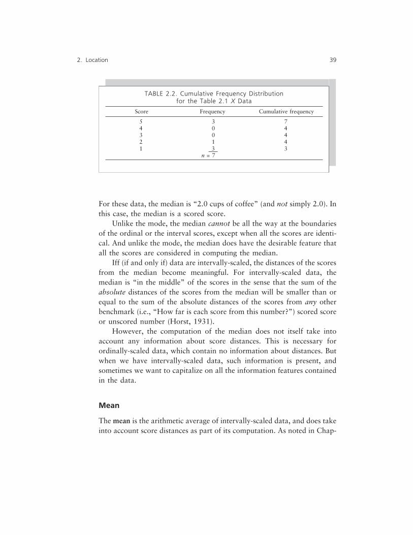
For these data, the median is “2.0 cups of coffee” (and not simply 2.0). Inthis case, the median is a scored score.

Unlike the mode, the median cannot be all the way at the boundariesof the ordinal or the interval scores, except when all the scores are identi-cal. And unlike the mode, the median does have the desirable feature thatall the scores are considered in computing the median.

Iff (if and only if) data are intervally-scaled, the distances of the scoresfrom the median become meaningful. For intervally-scaled data, themedian is “in the middle” of the scores in the sense that the sum of theabsolute distances of the scores from the median will be smaller than orequal to the sum of the absolute distances of the scores from any otherbenchmark (i.e., “How far is each score from this number?”) scored scoreor unscored number (Horst, 1931).

However, the computation of the median does not itself take intoaccount any information about score distances. This is necessary forordinally-scaled data, which contain no information about distances. Butwhen we have intervally-scaled data, such information is present, andsometimes we want to capitalize on all the information features containedin the data.

Mean

The mean is the arithmetic average of intervally-scaled data, and does takeinto account score distances as part of its computation. As noted in Chap-

2. Location 39

TABLE 2.2. Cumulative Frequency Distributionfor the Table 2.1 X Data

Score Frequency Cumulative frequency

5 3 74 0 43 0 42 1 41 3 3

n = 7

ter 1, the symbol for the mean is MX or X for sample data, and µX for pop-ulation data.

The formula for the mean of sample data is

MX = ΣXi / n (2.2)

where the Greek capital letter sigma (Σ) means “add them all up,” Xi arethe scores of each of the i individuals in the dataset, and n is the number ofscores in the sample. Note that MX does not have an i subscript, becausethe mean is one number representing the entire dataset, and may not evenbe any individual’s scored score in the data, and so the use of an i subscriptwould be inappropriate. The parameter formula for population data is

µX = ΣXi / N (2.3)

where N is the number of scores in the population.For the variable X Table 2.1 data, the sample mean, MX, equals

20.0/7, or to three decimal places, “2.857 cups of coffee.” Remember thatthe modes were “1 cup” and “5 cups,” and the median was “2.0 cups ofcoffee.” For these data, each of these three location descriptions yields adifferent answer, and so the selection of a particular location descriptionmight impact our interpretation of results even for a single dataset.

Of course, we are not limited to computing only a single locationdescriptive statistic, if our data are higher than nominally-scaled, andcomputing several helps us to understand our data. But typically scholarsreport only one such characteristic, perhaps because journal editors are soprotective of journal signature space. We will learn later in this chapterwhen some of these location results will be identical for a dataset, andwhen they will differ.

The mode is “in the center” in the loose sense of being some (any)scored score. The median, even for ordinally-scaled data, is “in the center”in the sense of dividing the ordered scores into two equal-sized groups oflower and higher scores. The mean is “in the center” in a physical sense ofbeing the fulcrum underneath the numberline at the point that the histo-gram would balance.

The mean has the property that if you subtract the mean from each ofthe scored scores, yielding deviation scores (symbolized by lowercase let-


ters, such as xi or yi), the deviation scores will always add up to exactlyzero (e.g., Σxi = 0.0). This implies that you could create a numberline bymarking equal intervals on a 2″-by-6″ board, possibly ranging from 0pounds to 12 pounds, and then place lead objects weighing between 0 and12 pounds at the corresponding locations on the board (e.g., a 3.5-poundobject at the location 3.5 on the board/numberline); the board (or seesaw/teeter-totter) would be level if placed on a fulcrum or balance point atwhatever location corresponded to the mean (e.g., “5.75 pounds” if thatwas the mean weight of the lead objects).

The mean also is “in the middle” of the scores in the sense that thesum of the squared distances of the scores from the mean will be smallerthan the sum of the squared distances of the scores from any other bench-mark (i.e., “How far is each score from this number?”) scored score orunscored number. These two characteristics of the mean make the mean agreat benchmark to use when we need to compare each score to some onebenchmark number to help characterize dynamics within our data.

Rounding

When dividing or multiplying numbers, it is possible to obtain answersthat are nonterminating. For example, 2 divided by 3 yields a nontermina-ting result. There are two options for reporting nonterminating results.First, the nonterminating number or set of numbers can be represented byplacing a line over the nonterminating values. For example, 2 divided by 3can be reported as 0.66. Second, rounding can be employed withnonterminating numbers, just as rounding can be employed with any deci-mal values in real numbers.

In the social sciences, descriptive statistics are rarely reported to morethan either two or three decimal values, partly because for most of ourvariables extremely small differences are not meaningful or noteworthy.For example, it is usually sufficient to compute the mean number of rightanswers on a test as 57.6 or 57.63, but it probably makes no sense toreport the mean as “57.63289366567 right answers.” The “289366567”part of the number is trivial.

Reporting an excessive number of decimal values communicates moreprecision than is really present in most data. However, when our descrip-

2. Location 41

tive statistics can be employed by others to replicate our analyses (as in atextbook), or to conduct analyses different than ours (because some sec-ondary analyses do not require the original data), then more decimal val-ues may be used in reporting.

Rounding requires, first, a decision about the desired number of deci-mal places (e.g., two). Then one rounds from the number at the decimalplace immediately beyond the targeted number of decimal places (e.g., thethird decimal place). If the number we are rounding from is less than 5, weround down (e.g., 3.744 becomes 3.74 if we are rounding to two decimalplaces). If the number we are rounding from is greater than 5, we roundup (e.g., 3.746 becomes 3.75 if we are rounding to two decimal places).

When the number we are rounding from is a 5, special rules apply(Tukey, 1977). There are nine possible numbers in the location fromwhich we are rounding where rounding may be necessary (i.e., 1, 2, 3,. . . , 9). Arguably, rounding is not being performed when in a descriptivestatistic a zero is to the right of the targeted number of decimal places.

When we are rounding from descriptive statistics, four numbers arebelow 5 and four numbers are above 5. To avoid rounding from 5, andconsistently biasing rounded results upward or downward, we round halfthe time from 5. Specifically, we round up if the rounded number willbecome even (e.g., 3.735 becomes 3.74), and we do not round up if doingso would make the rounded number odd (e.g., 3.745 becomes 3.74).

Purpose of Division

In addition to rounding, division also requires some explanation. Let’sconsider the formula for the sample mean, MX = ΣXi / n, and why wedivide by n, and especially what function division serves in statistics.

Presume that we have data about the life savings of a sample ofwomen and a sample of men. If we were interested in the wealth of thetwo groups as a whole, we could compare the sums of the savings in thetwo groups. But if we are interested instead in savings from the perspectiveof the individual people of both genders, we need to compare locationdescriptive statistics, such as means, rather than score sums.

If the groups were not of equal size, and the sum of the savings of thesmaller group was larger than the sum of the savings of the bigger group,


we could be unequivocally certain that the smaller group had more savingsthan the larger group, even given a focus on the perspective of the individ-ual. Of course, we still could not quantify how much more savings therewere in the more frugal group. Conversely, if the groups were not of equalsize, and the sum of the savings of the bigger group was larger than thesum of the savings of the smaller group, we could not be certain that fromthe individual perspective the bigger group had more savings than thesmaller group.

If the two groups were exactly equal in size, we could compare thesums to make accurate judgments of wealth from both the group and theindividual perspectives. But researchers do not limit themselves to study-ing groups that are always of equal size.

We need ways to compare data dynamics represented in descriptivestatistics that will work when group sizes are equal, but also will workwhen group sizes differ. Happily, statisticians know that when we divide,we are removing from our answer that which we are using to divide.

Most statistics formulas involve division that uses some function of n(either n or n – 1), so that results may be compared across groups of dispa-rate sizes. And sometimes we divide by other data characteristics, so thatthese too no longer impact our answers.

Of course, some analyses focus exclusively on the data in hand, at ourfixed single sample size. For analyses of this sort, division by n (or n – 1) isunnecessary, because the sample size is a constant for within-study charac-terizations of data.

Outliers

The mean is fundamentally important in computing other characteriza-tions of data in addition to location (i.e., dispersion, shape, and relation-ship), as we shall see in succeeding chapters. However, the mean is verysensitive to anomalous or outlying scores. And any distortions in the meanunavoidably also impact the characterizations of data that themselvesinvoke the mean as a benchmark reference point.

An outlier is a participant whose data are distinctly atypical and thuswould unduly influence characterizations of the data. Some researchershave the misconception that outliers are evil people (or lab rats, etc.) who

2. Location 43

are or should be branded on their foreheads with giant, red capital letter“O’s.”

Instead, most people are outlying in some sense on at least some vari-ables. We are all probably really exceptionally bad, or exceptionally good,or weird, on some things. This is part of the challenge of formulatingsocial science generalizations involving people with so many individualdifferences. Of course, some people may be outliers on more variablesthan other people.

To complicate matters, as we shall also eventually see, an outlier is notnecessarily outlying on all descriptive statistics for a given dataset. Forexample, a given person may be an outlier regarding the mean, but notregarding the median or other statistics.

Table 2.3 illustrates these dynamics. Jane is not an outlier regardingthe mean or the median on X1. However, Jane arguably is an outlierregarding the mean of X4, even though she is not an outlier regarding themedian of X4.

The Table 2.3 data illustrate the relative sensitivities to outliers of themean versus the median. The mean can be very highly influenced by rela-tively few anomalous scores in the data, even when the number of scores isquite large.

However, the sensitivity of the mean to unusual scores does not sug-gest that the median is always a better location statistic than the mean. Insome cases, we care more about people who are extreme (e.g., peoplewhose cholesterol is exceptionally high) and therefore would intentionally


TABLE 2.3. Heuristic Data IllustratingImpacts of Outliers on M and Mdn

Participant X1 X2 X3 X4

Robert 1 1 1 1David 2 2 2 2Karan 3 3 3 3Jane 4 9 9 999

Median 2.50 2.50 2.50 2.50Mean 2.00 3.75 26.25 251.25

select the mean as a descriptive statistic most sensitive to the most or leastworrisome scores.

When the researcher is in a quandary about which central tendencydescription to use, remember that this is not necessarily an either-orchoice. It may be perfectly reasonable to report several location descriptivestatistics to more fully represent the scores, and to give readers a morecomplete understanding of the data.

Another alternative is to use more sophisticated and considerablymore complex central tendency descriptive statistics. For example, theHuber (1981) estimator can be used. Statistically, this estimator for sam-ple data in essence focuses on the mean for the core of the data distribu-tion and on the median for more extreme portions of the distribution(Maxwell & Delaney, 2004).

The Huber estimator is not computed using a formula! In particularlysophisticated statistics, sometimes no formula is present. When no for-mula exists to derive an estimate, computationally-intensive proceduresrequiring computers, called “iteration,” sometimes can still produce anestimate. Iteration is a statistical routine in which a first guess is made,then the guess is repeatedly tweaked using some statistical rule, until a sat-isfactory estimate is obtained. For example, in the method called explor-atory factor analysis, iteration is always performed as part of what iscalled rotation (Thompson, 2004).

The mechanics of iteratively guessing the Huber estimator for adataset are beyond the scope of the present treatment. The point is thatthere are a lot of descriptive statistics that can be used to characterize loca-tion, and no single characterization is always definitively correct.

A related question is what to do with the outliers themselves. Perhapsthe better solution for dealing with outliers, rather than changing thedescriptive statistic, is to eliminate or alter the scores of outliers.

The first thing to consider when encountering outlying scores is thatdata may have been incorrectly entered. Out-of-range values (e.g., an IQscore of 900) are obvious indications of inaccurate data entry. Out-of-range or other entry errors are simply corrected once the mistakes areidentified.

Second, further investigation may shed some light on whether plausi-ble but unlikely scores are legitimate values. For example, perhaps agrade-equivalent score of 7.2 by a doctoral student on a reading skills test

2. Location 45

is possible, but the alternative hypothesis—that the student was not work-ing to capacity—clearly must be considered. Upon being interviewed, thestudent might confess lack of motivation when taking the test. Or consul-tation of other data for the student (e.g., a GRE verbal score of 780) mightsuggest that the student simply was not trying. When external informationdefinitively indicates that scores are inaccurate, participants might beretested or their scores simply may be omitted from the dataset.

Third, when scores are in some sense extreme but possible, and noexternal evidence can explain the basis of the anomaly, decisions aboutwhat to do with the outlying scores become quite difficult. In general,omitting outliers simply because they are bothersome, without theoreticaljustification, is unreasonable. As Pedhazur and Schmelkin (1991) noted,“the onus of interpreting what the outliers and/or influential observationsmean in a set of data and the decision about what to do is, needless to say,on the researcher” (p. 408). Researchers should avoid the temptation foratavistic escape inherent in using arbitrary cutoffs for degrees of scoreextremity as the sole basis for removing unexpected scores (Johnson,1985).

One prudent choice may be to report results for analyses both withand without the outliers with plausible scores for whom the basis for scoreextremity cannot be discerned. If the interpretations are reasonably invari-ant (i.e., similar) across analyses, the researcher is assured that conclusionsare not artifacts of analytic strategies.

�� Four Criteria for Evaluating Statistics

As suggested by the previous discussion, no statistic provides a perfectcharacterization of sample scores under all circumstances. But method-ologists have elaborated four criteria to guide evaluations of how well sta-tistics work.

Sufficiency refers to whether a statistic makes use of all the data in thesample. For example, the mode is not a sufficient statistic, except in verysmall samples (i.e., n = 2) or when the scores delineate a constant ratherthan a variable. The median and the mean, on the other hand, are suffi-cient statistics.


Unbiasedness refers to the capacity of repeated samples invoking astatistic to yield accurate estimates of corresponding parameters. Forexample, M is an unbiased estimate of µ. If we draw infinitely many ran-dom samples, each of a given size (e.g., n = 50) from a population, andaverage the sample Ms, that average will equal µ.

Efficiency refers to how tightly statistics used to estimate parameterscluster around the actual parameters. For example, if we are attempting tocharacterize the parameter central tendency, we prefer estimates using agiven sample size that fluctuate less across samples from a given popula-tion than do other plausible estimates.

Robustness refers to the capacity of a statistic to be less influenced byoutlying scores. For example, as noted previously, although the mean is asufficient, unbiased, and relatively efficient statistic, the mean is moreinfluenced by outliers than is the median.

�� Two Robust Location Statistics

Statisticians have long been concerned about how to improve character-izations of data containing outliers. For example, in a short, accessiblearticle, Wilcox (1998) argued that a good deal of educational and psycho-logical research probably has reached erroneous conclusions based onoverreliance on classical statistics such as the mean.

Robust statistics are variations on older classical estimates (e.g., MX,MdnX) for location and other data descriptions that seek to minimize theinfluences of outliers. Wilcox (1997) published a book on robust statisticsalternatives. Also see Keselman, Kowalchuk, and Lix (1998) andKeselman, Lix, and Kowalchuk (1998). Table 2.4 presents a heuristicdataset that can be used to illustrate two alternative “robust” locationdescriptive statistics that can be employed to mitigate the disproportionateinfluences of extreme scores.

One robust method “winsorizes” (à la statistician Charles Winsor) thescore distribution by substituting less extreme values in the distributionfor more extreme values. For example, in a set of 20 skewed scores, thefourth score (e.g., 433) may be substituted for scores 1 through 3, and inthe other tail the seventeenth score (e.g., 560) may be substituted for

2. Location 47

scores 18 through 20. The mean of this winsorized distribution (e.g., MX′ =480.10) thus becomes less extreme than the original value (e.g., MX =500.00).

Another robust alternative “trims” the more extreme scores and thencomputes a “trimmed” mean. In this example, 0.15 of the distribution istrimmed from each tail. The resulting mean (e.g., MX = 473.07) is therebycloser to the median of the original distribution, which has remained461.00.

In a sense, as pointed out by Lunneborg (1999), the median can itselfbe thought of as a trimmed mean (i.e., a mean based on trimming essen-tially 50% of the scores from both tails). In theory, robust statistics may


TABLE 2.4. Two Illustrative “Robust” Location Descriptive Statistics

ID X X′ X

1 430 433 —2 431 433 —3 432 433 —4 433 433 4335 435 435 4356 438 438 4387 442 442 4428 446 446 4469 451 451 451

10 457 457 45711 465 465 46512 474 474 47413 484 484 48414 496 496 49615 512 512 51216 530 530 53017 560 560 56018 595 560 —19 649 560 —20 840 560 —

M 500.00 480.10a 473.07b

Mdn 461.00 461.00 461.00

aThe arithmetic average of the third column, containing one version of altered data, is thewinsorized mean.bThe arithmetic average of the fourth column, containing data omitting 0.15 (or 15%) of thescores in both extremes of the distribution (n = 20 – 3 – 3 = 14), is the trimmed mean.

generate more replicable characterizations of data, because at least insome respects the influence of more extreme scores, which given theiratypicality may be less likely to be drawn in future samples, has been mini-mized.

However, robust statistics have not been widely employed in contem-porary research. Perhaps scholars who are not methodologists have diffi-culty keeping up with the burgeoning literatures in their own disciplines,much less the burgeoning methodology literature. Or some researchersmay hesitate to report methods not already routinely presented in jour-nals, for fear that if they violate normative expectations for scholarlybehavior their work may be less likely to be published.

Some Key Concepts

All location or central tendency statistics, to be reasonable, must fallwithin the score distribution and ideally, in one sense or another,should fall near the center of the distribution. Location statistics canbe very useful in understanding and explaining the story underlyingour data.

However, too often researchers focus solely on location statistics,and especially the mean. And, as we shall see in our Chapter 4 treat-ment of shape statistics, the median is too infrequently considered. AsGrissom and Kim (2005) noted, sometimes a “sample’s [emphasisadded] median can provide a more accurate estimate of the mean ofthe population [emphasis added] than does the mean of that sample”(p. 40).


1. Consider the scores {1”, 1”, 2”, 3”, 8”}. Determine the mean and the

median. Because these data are intervally-scaled, the differences of scores

from both the mean and the median are meaningful. Compute (a) the dif-

ference, (b) the absolute difference, and (c) the squared difference of

each score from the median. Then sum up each set of three numbers.

Then compute (a) the difference, (b) the absolute difference, and (c)

the squared difference of each score from the mean. Then sum up each

set of three numbers.

2. Location 49

What are the sums of the difference scores from the mean, and from

the median? Which descriptive statistic, mean or median, has the smallest

sum of the absolute difference scores? Which descriptive statistic, mean

or median, has the smallest sum of the squared difference scores?

2. Researchers not infrequently encounter missing data (e.g., some students

skip certain test questions, or some participants were absent when a

given test was administered). Even though there are better ways to deal

with missing data (Little & Rubin, 1987), sometimes researchers substi-

tute the mean of the nonmissing scores on a variable for the missing data

on a given variable. What effect does using this mean imputation for

missing data have on the means computed both before and after the sub-

stitution is performed?

Imputation of missing data can be particularly problematic when the

data are not missing at random. A classic example involves statistician

Abraham Wald’s work on aircraft survivability in World War II (Mangel &

Samaniego, 1984). Researchers counted the bullet and shrapnel injuries

in various locations on returning aircraft. Might a focus on reinforcing the

locations on returning aircraft receiving the most hits have been less pro-

ductive than focusing on the locations receiving the most hits on the

planes that did not return? Of course, damage data for nonreturning

planes was not available to the analysts, and Wald was merely emphasiz-

ing that the researchers really did not have access to the data they most

needed, and should have been more cautious in using the data that were

available!

3. For two independent and equally critical reasons, the influences of addi-

tive and multiplicative constants on statistics ought to be understood.

First, to understand various statistics (e.g., medians, means), we must

know what causes or affects them, and what does not. Second, through-

out statistics, as we shall see in subsequent chapters, additive and/or

multiplicative constants are used. To understand the results invoking

these constants, we must understand the impacts of additive and multipli-

cative constants.


Consider the following data:

Y X1 X2 X3

Jane 1 1 0 6

Douglas 2 2 0 1

Jim 3 3 0 1

Mike 4 4 4 1

Compute the mean of each variable. Then apply the following con-

stants to X1, X2, and X3, and next compute the means of the various

new versions of the three variables:

a. Add 3 to each score.

b. Add –1 to each score.

c. Multiply each score by 2.

d. Multiply each score by –0.5.

e. First add –1 to each score; then multiply each result by 2.

For each original and revised version of a given variable, plot the origi-

nal values of a given variable in a histogram in blue or black pen, and plot

the revised values of a given variable in a histogram in red or green pen.

How do the distributions move as constants are applied? How does the

mean move in relation to its score distribution?

What rule can we formulate to express the effects on means of addi-

tive constants (e.g., “New mean always equals original mean . . .”)? What

rule can we formulate to express the effects on means of multiplicative

constants (e.g., “New mean always equals original mean . . .”)? Why

mathematically do these rules work? When will a multiplicative constant

not change the value of the original mean?

2. Location 51

3

Dispersion

Dispersion or “spreadoutness” statistics quantify the answer to thequestion, “How dissimilar (or similar) are the scores to eachother?” Dispersion statistics can be used for two purposes: (a) tocharacterize how well location descriptive statistics perform at

representing all the data, and (b) to characterize score “spreadoutness” asan important result in its own right.

Of course, the dispersion question only makes sense in the presence ofdata that are at least intervally-scaled. With nominal or ordinal data, all wecan do is compute the proportion 0.0 to 1.0 (or the percentages 0% to100%) of scores within the modal score category. This is a crude dispersioncharacterization, but does not quantify how much the scores differ. But fornominal or ordinal data, how could we quantify how distant scores are fromeach other, or from some benchmark, if the scores have no meaningful,nonarbitrary information about distance on a “ruler” that is at leastintervally-scaled?

53

�� Quality of Location Descriptive Statistics

Recognizing that location descriptions may differ in their quality, and evenhave no value for some data, is a fundamentally important understanding.For example, presume that you and your significant other are sitting undera tree on a university park bench. Lo and behold, along comes Bill Gates,the chairperson of Microsoft Corporation.

The accumulated savings of the three of you in dollars could be mea-sured, and the data would be intervally-scaled. Thus, the mean could becomputed. But would the resulting one number fairly represent all, or evenany, of the three scores? Mr. Gates might be perturbed that the mean woe-fully underrepresented his net worth. And you might be depressed to real-ize that the mean of the group was (presumably) so far above your ownlife savings.

As noted in Chapter 2, all the central tendency statistics work per-fectly well for data that have zero dispersion. But location descriptionswork less well as scores become increasingly dissimilar from each other.And at some degree of dispersion, the concept of central tendency becomessenseless. The big picture becomes only the score spread, and not the useof one number to represent all the scores.

But for other data for which central tendency is sensible and that areat least intervally-scaled, dispersion statistics are essential quantificationsof the quality of location descriptions. The important implication is:Never report a central tendency statistic (e.g., MX) without reporting (usu-ally in parentheses) right next to the location description a dispersiondescription.

�� Important in Its Own Right

Dispersion statistics can also be important in their own right. In suchcases, these dispersion characterizations might be presented without evenreporting central tendency descriptions.

Consider the results below for 10 first graders coincidentally allnamed after deceased former U.S. presidents. The students were ran-domly assigned to one of two methods of teaching spelling. Prior to


intervention, the students completed a pretest on which the number ofcorrectly-spelled words was recorded. After instruction, the studentsagain completed a brief posttest measuring the number of correctly-spelled words.

Group / first grader Pretest Posttest

ControlM. Fillmore 1 1R. Hayes 2 2C. Coolidge 3 3H. Hoover 4 4R. Nixon 5 5

M 3.0 3.0

ExperimentalG. Washington 1 0T. Jefferson 2 0A. Jackson 3 3A. Lincoln 4 6F. Roosevelt 5 6

M 3.0 3.0

The means for these data suggest that the process of randomly assign-ing participants to groups effectively created groups that were equivalentat the start of the intervention, reflected in part by the fact that both pre-test means equaled “3.0 correct answers.” That is the good news. The badnews is that the two posttest means suggest that the interventions wereequally (in)effective.

However, upon closer scrutiny, the data do suggest interventioneffects, albeit not on average achievement. Here the new, experimentalteaching method caused student achievement to become increasingly dis-persed. Clearly, understanding intervention effects requires more thanlooking only at group means.

The outcomes for these data (no mean change, but increased achieve-ment variability) are obvious given that the dataset in the example is ridic-ulously small. This sort of impact might have been obscured in a large

3. Dispersion 55

dataset, and might have gone completely unnoticed by researchers whosadly have “obsession with only means” personality disorder.

The pattern here of no growth during educational intervention is nottypical. But the pattern of interventions impacting score spread is reason-ably common. Indeed, educational interventions frequently yield “fan”spreads reflecting differential impacts for students starting at different lev-els. Figure 3.1 illustrates such a “fan” effect for the five participants in theintervention group whose scores became more dispersed following theintervention.

Less able students over the course of intervention may stay about thesame or only slightly improve. More able students may not only improve,but may even improve more dramatically than their less able counterparts.This dynamic reflects the fact that pretest achievement scores involve esti-mated abilities at a given point in time, but may involve as well differentialrates of learning.

The challenge in many educational interventions is not only to helpstudents learn, but also to impact rates of learning. The take-home mes-sage is to remember that means only characterize one aspect of data, andthat other characterizations of data dynamics may also be important, ormay even be more or most important.


FIGURE 3.1. Plot of pretest to posttest changes for intervention participants

�� Measures of Score Spread

Expectations for Dispersion Statistics

The least “spreadout” that scores could be would occur if all the scoreswere identical, regardless of what the identical scores were. In this case,the scores would have exactly zero spread. We expect statistics describingscore variability or dispersion to all yield numerical answers of exactlyzero (i.e., 0.00) when the scores have no spreadoutness.

A negative numerical answer for any statistic describing dispersionwould assert that “the scores are less ‘spreadout’ than the scores would beif the scores were all identical.” This does not seem plausible!

When any two scores differ from each other, we expect dispersiondescriptive statistics to be greater than zero. As scores are increasinglymore dissimilar to each other, we also expect statistics describing scorevariability to increase in value.

Logically, because scores can take on infinitely many different values,the scores can also be infinitely dispersed from each other. Therefore,there is no universal mathematical limit on the upper-bound or maximumvalues of descriptive statistics for dispersion.

Range

The simplest descriptive statistic that characterizes score dispersion is therange. The range is the largest score minus the smallest score. We cannotcompute the range for nominal data, because the scores of the variable’scategories have no meaningful order, so there is no highest or lowest. Wecannot compute the range for ordinal data, because addition or subtrac-tion is not reasonable unless the scores are intervally-scaled.

The range has the expected feature that we obtain zero if all the scoresare identical, in which case we subtract any one person’s score from anyone other person’s score to compute the range. The range is nonzero if anytwo people have different scores, as reasonably expected of all dispersionstatistics.

The range, like all the location descriptive statistics, is in the score

3. Dispersion 57

world. So, if the scores are {$1.00, $3.00, and $5.00}, the mean is not 3.0,but $3.00. Similarly, the range would be $4.00.

The range has the disadvantage that only two scores are considered inits computation. This means that different datasets, each involving differ-ent score variabilities, may nevertheless have the same range. For example,the following three datasets (years 2006, 2008, and 2010) all have a rangeof $2M, even though the datasets differ in spreadoutness, going from leastdispersion in the 2006 data to the most dispersion in 2010.

Person 2006 2008 2010

George $2M $2.0M $2MWenona $0 $1.5M $2MSteve $0 $1.0M $2MPatty $0 $1.0M $0Judy $0 $0.5M $0Sheri $0 $0 $0

Of course, the insensitivity of the range to all but two scores is com-pletely irrelevant at every sample size, if the scores are a constant, and sothe range equals zero. So, for example, at n = 1,000,000, for range = 0.0,this descriptive statistic does a perfect job of characterizing the dispersionof all 1,000,000 scores.

However, for scores that constitute a variable, the range is less andless satisfactory as n increases, because more and more scores are ignored,or because data with different dispersions can have the same ranges. Weneed a dispersion descriptive statistic that considers every score and yieldsa different result for datasets with different “spreadoutness.”

Sum of Squares

If we wish to compare each score with every other score, there would be[n(n – 1)] / 2 pairwise comparisons. For example, for the previous data,involving the scores of six people, there are [6(6 – 1)] / 2 = [6(5)] / 2 = 30 / 2= 15 unique comparisons. As a starting point, we could compute how farevery score deviated from George’s score, and then add up or average the“George deviations.”

Which person we use as the benchmark score makes no difference. If


all the scores are the same, the sum of the “George deviations” or the“Wenona deviations” or any of these deviations will be zero, and the aver-age of these will then also be zero. Alternatively, we could use any number(e.g., 0.0) as the comparative benchmark, even a number outside the scorerange.

However, as noted in Chapter 2, the mean has some very special prop-erties. For example, M is “in the center” of the scores, even in the sensethat physical weights balance on a fulcrum positioned at M. These proper-ties of the mean make the mean particularly desirable as our benchmarkfrom which we may measure dispersion for each score.

One candidate for a descriptive dispersion statistic is the sum of theindividual deviation scores from the mean, where each xi = Xi – MX. TheΣxi = 0.0 when the data constitute a constant, which is desirable. The sumof the deviation scores also has the desirable feature of considering eachand every score. However, the sum of the deviation scores would be acompletely unsatisfactory measure of score dispersion, because Σxi isalways zero, even for variables, as emphasized in Chapter 2.

One alternative would be to compute the sum of the absolute devia-tions from the mean or some function of this sum, such as the mean abso-lute deviation (i.e., MADX = Σ|xi| / n). For example, for the scores {$1, $3,and $5}, the sum of the absolute deviations is |–$2| + |$0| + |$2| = $2 + $0+ $2 = $4. And MADX = $4 / 3 = $1.33. This description of dispersion isnot unreasonable, but the description is rarely used because this character-ization lacks a statistical “theoretical undergirding,” and “the mathemati-cal statistician finds the process of ‘taking absolute values’ presents specialdifficulties for certain mathematical derivations” (Glass & Stanley, 1970,p. 86).

Another alternative is to square the deviation scores, and then sum thesquared deviations. Doing so yields the sum of squares (SOSX). For exam-ple, the SOS of the following three IQ scores is 200.0:

Person Xi – X = xi xi2

Geri 125 – 135 = –10 100Murray 145 – 135 = 10 100Wendy 135 – 135 = 0 0

Σxi 0SOSX 200

3. Dispersion 59

Thus, the formula for the SOSX can be expressed as

SOSX = Σ(Xi – X)2 (3.1)

or equivalently as

SOSX = Σ xi2 (3.2)

An algebraically equivalent formula uses the original scores (or “rawscores”) rather than the mean and the deviation scores:

SOSX = ΣXi2 – [(ΣXi)2 / n] (3.3)

For our data we have [1252 + 1452 + 1352] – [(4052) / 3] = [15625 + 21025+ 18225] – [164025 / 3] = 54875 – 54675 = 200. The “raw score” for-mula is computationally easier. However, computational ease of use wasmore relevant when statistics were computed on hand-cranked calcula-tors. And the raw score formula has the very serious heuristic downsidethat the formula completely obscures (a) the underlying nature of SOS and(b) the role of the mean in computing several dispersion statistics.

The sum of squares cannot be negative, because of the squaring opera-tion. The SOS will be zero iff (if and only if) the scores constitute a con-stant. The SOS will be nonzero for all variables and, for a fixed n, willbecome larger as scores become more dissimilar from each other. Concep-tually, the SOS is information about both the amount and the origins ofindividual differences.

The social sciences presume that people differ as individuals. Theseindividual differences create challenges in formulating theoretical general-izations, and may make universal statements impossible. Even medicinesdo not work equally well in different people! But these individual differ-ences are exactly the focus of scholars in the social sciences. Thus, our def-inition of the SOS makes the SOS sound critically important inquantitative research in the social sciences, because the SOS indeed is criti-cally important in quantitative research.

As we shall see, the SOS has some limitations as a descriptive statistic.However, the SOS is used ubiquitously in various other statistical analy-ses, as will be illustrated over and over again in later chapters.


The SOS in this case quantifies the amount of information we have inour data as “200.0 squared IQ points.” In general, we prefer more ratherthan less information (i.e., variability) about the variables of interest to us.If we are investigating childhood depression, and the SOS of the depres-sion scores of our study participants is zero, we will have considerable dif-ficulty (actually, an impossibility) in understanding the nature and causesof depression.

But a nonzero SOS can also be used to explore the origins of ourinformation about individual differences. First, we can partition the SOSinformation based on the degree to which the scores are reliable, and thedegree to which the information is unreliable. This is a measurement studyapplication that focuses on score psychometric integrity, and is beyond thescope of the present treatment, but the interested reader is directed toDawson (1999) or Thompson (2003).

Second, we can perform a “who” partition of our information.Because each person’s contribution to our information is unique, nonover-lapping, or uncorrelated, xi

2 for a given person quantifies how much infor-mation a given study participant contributed to the dataset. We can evensecure graph paper and draw a Venn diagram, portraying the informationby using different color pens for each participant.

In the present example, we will draw in red a rectangle or square con-taining 100 graph paper boxes to represent Geri’s contribution. We candraw a contiguous rectangle or square in blue to represent Murray’s con-tribution of 100 area world units of information. We can draw Wendy’scontribution in chartreuse, but here there will be no problem if we do nothave this color of pen, because Wendy contributed no information aboutindividual differences on this particular variable. Persons scoring at themean never contribute any information about individual differences, atleast on this given variable.

Third, we can perform a substantive partition to explore how our 200squared units of information originated, or how well other variables mightpredict or explain our information. Substantive partitioning applicationsare the focus of the “Bivariate Relationships” chapter in this book and ofall subsequent chapters.

The mean of our three IQ scores is “135 IQ points.” However, thesum of squares is not “200.0 IQ points.” Instead, the SOSX is “200.0squared IQ points.” In other words, although the three scores and the cen-

3. Dispersion 61

tral tendency descriptive statistics for the scores are all in the “score”world, the sum of squares is the first statistic we have encountered that isin the squared or “area” world.

�� Variance

The SOS meets many of our expectations for a dispersion descriptive sta-tistic and has many, many uses in applications that are not descriptive(e.g., that are explanatory or substantive). The SOS is quite useful inquantifying how much information we have on a given variable in a studywith a fixed number of participants to the extent that we focus only on agiven dataset.

However, problems may arise if we wish to compare score spreadacross subgroups within our study, or if we wish to compare dispersion ofscores in our study with score dispersion in some other study. We cancompare score spreads apples-to-apples using SOS if the scores in thegroups are all constants, and the sums of squares are all zero.

But if the scores create a variable (SOS > 0.0), there may be difficul-ties. If two groups (or subgroups) of scores involve exactly the same num-ber of participants, we can (a) make definitive statements about which setof scores is more dispersed and (b) quantify in squared information unitshow different dispersion is by subtracting the smaller SOS from the largerSOS.

If two groups have different numbers of participants, and the SOS inthe smaller group is larger than the SOS in the larger group, we can be cer-tain that the scores are more dispersed in the smaller group than in thelarger group. However, we cannot quantify the amount of differentialscore dispersion on the average by subtracting the sums of squares onefrom the other, because this computation would not recognize the differ-ence in the group sizes.

Things are particularly problematic if the SOS for the variable in thelarger group is larger than the SOS in the smaller group. Now we cannotdetermine whether the larger group’s SOS is due to (a) cumulating squareddeviation scores over more participants, (b) greater average dispersion in


the larger group, or (c) both these factors. Nor can we quantify theamounts of differential average score spreads in the two groups.

As explained in Chapter 2, these problems can be overcome by remov-ing the influence of group size from our descriptive statistic via division.At first impression, the solution seems very straightforward: Divide by nfor samples, and N for populations. Unfortunately, the correct solution isa bit more complex.

Dividing the SOS by a function of the number of participants yields anarea-world descriptive statistic, the variance. The parameter symbol forthe population variance is σ2

X. The statistic symbol for the sample vari-ance is VarX (or SD2

X, for reasons that will become clear in the next sec-tion).

However, it turns out that we must use different divisors, dependingon whether our data constitute a population or a sample. For the parame-ter, we use the formula

σ2X = SOSX / N (3.4)

For the statistic, we use

VarX = SD2X = SOSX / (n – 1) (3.5)

Obviously, the variance cannot be computed for sample data with n = 1,because division by n – 1 = 0 is impermissible, but dispersion is a mootpoint of little or no interest when n equals 1 anyway.

Note that dividing by n – 1 rather than by n for sample data willalways result in a larger answer, iff SOS ≠ 0. The difference in our resultfrom dividing by n – 1 versus n (iff SOS ≠ 0) is fairly dramatic when n issmall (e.g., when n is 2 or 3). How much larger our answer will be, how-ever, iff SOS ≠ 0, differs for every value of n. This dynamic is illustrated bythe following list of potential values for n:

n n – 1 Difference

2 1 50.00%3 2 33.33%4 3 25.00%

3. Dispersion 63

5 4 20.00%6 5 16.66%7 6 14.28%8 7 12.50%9 8 11.11%

10 9 10.00%100 99 1.00%

1,000 999 0.10%1,000,000 999,999 0.0001%

Division by n – 1 rather than by n is a correction for statistical biasthat would otherwise occur in our answer. Problems of systematic bias inresearch present no difficulty as long as we (a) recognize that bias is pres-ent and (b) know the appropriate correction factor.

For example, people may have a tendency to either lie or uncon-sciously exaggerate how much money they earn, how often they go tochurch, or how often they have sex. When we are conducting door-to-door surveys, if we know the correction factor is to divide by 2, there issimply no point in confronting the study participant for being dishonestwhen we knock on the door, and pose our research question, and theyrespond “eight times per week.” We simply record 4.0 on our data collec-tion form and move on to the next house, hoping that we will not getpunched in the nose for asking intensely personal questions.

Similarly, statistical bias in estimating score dispersion in sample datais not problematic as long as we know the “fix.” When we are characteriz-ing score dispersion in the sample, we are using the statistic as an estimateof the population dispersion. Samples always imply ultimate interest in thepopulation. Otherwise, we would instead call the data the population, anduse Equation 3.1. But why do sample data tend to underrepresent thescore dispersion present in the population, when we are drawing strictlyrandom samples from the population?

The tendency of sample data to underrepresent score dispersion in thepopulation is actually conditional on the shape of the population data, atopic covered in more depth in Chapter 4. However, for now, let usassume that the population consists of the nine scores portrayed in the Fig-ure 3.2 histogram of the Table 3.1 data.

On each successive selection from the population when creating the


sample, each person’s probability of being drawn is exactly equal, by defi-nition of what simple random sampling means. For example, the probabil-ity of drawing Molly first is 1 / 9, the probability of drawing Geri is 1 / 9,and the probability of drawing Wendy is 1 / 9. After the first draw, on thesecond draw, every person’s probability of being selected is now exactly1 / 8.

But (and this is a very big “but”), the probability of drawing each ofthe five scores is not equal. The probability of drawing scores 1 or 5 is1 / 9 each. But the probability of drawing scores 2 or 4 is instead 2 / 9each. And the probability of drawing score 3 is 3 / 9, or 1 / 3.

This means that random samples from populations such as that por-trayed in Figure 3.2 tend to overrepresent scores in the middle, andunderrepresent scores in the two extremes. Consequently, scores in ran-dom samples for populations like this one tend to be less dispersed thanthe populations from which the samples are drawn! This is the dynamic

3. Dispersion 65

TABLE 3.1. Population Scores (N = 9)

Person X

Molly 1Geri 2Murray 2Peggy 3Carol 3Anne 3Donna 4Deborah 4Wendy 5

FIGURE 3.2. Histogram for a population consisting of nine scores

for which we are correcting for bias by dividing by n – 1 rather than by nwhen we have sample data.

Standard Deviation

The variance meets our expectations for describing score spread. The vari-ance (like every other dispersion statistic) can be no less than zero and iszero iff the scores are a constant. The variance gets larger as scores becomemore dissimilar to each other (or differ more from a score benchmark, themean). And the variance can be used to compare score dispersion acrossgroups of unequal sizes, even when the scores are not a constant.

Of course, the variance is in a squared metric (e.g., “580 squaredpesos,” “76 squared pounds,” “350 squared IQ points”). Mathematically,this poses no difficulty. However, most of us are more comfortable work-ing in the unsquared metric of the score world. For example, if we ask astore clerk whether 100 squared dollars is sufficient to pay for our pur-chase, the clerk may look at us quizzically, and we may even be arrested.

Taking the square root of the variance puts our descriptive statisticback in the score world, and in the metric of the original score. The squareroot of the variance is the standard deviation (i.e., σX for the parameter,and SDX for the statistic). The parameter formula is

σX = SQRT[σ2X] = [SOSX / N]0.5 (3.6)

Note that raising a value to the exponential power of 0.5 is equivalent totaking the square root of the value. The statistic formula is

SDX = SQRT[VarX] = [SOSX / (n – 1)]0.5 (3.7)

Thus, if the scores are measured in the units of number of correct testanswers, and the variance is “4.0 squared correct answers,” the standarddeviation would be “2.0 correct answers.”

We have noted previously that the mean has some special features as ameasure of central tendency, including the fact that Σxi = 0.0. The mean isused as the benchmark from which we quantify degree of score dispersion.


We initially invoke a squaring function to quantify score spread from themean. Consequently, the standard deviation is sometimes called the “firstmoment about the mean.” Other descriptive statistics also use the mean asthe benchmark from which to quantify deviations, but use higher-orderexponential powers of the deviations (i.e., 3 and 4), thereby defining thesecond and third moments about the mean. These two additional statisticsare presented in Chapter 4.

�� Situation-Specific Maximum Dispersion

Deep understanding of statistical characterizations of data requires insightinto what expectations ought apply to different results, and what universallimits (e.g., minimum possible results) apply for various descriptive statis-tics. Understanding also requires knowledge of situation-specific mathe-matical restrictions on possible results.

For example, dispersion descriptive statistics have a universal mathe-matical lower-bound limit. Dispersion statistics cannot be less than zero,and will be zero only for data that constitute a constant.

Dispersion statistics have no universal mathematical upper-boundlimit. For example, SOS can equal 1,000,000,000, and SD can equal1 × 1027. But dispersion statistics do have an upper-bound mathematicallimit if we constrain the description as regards (a) how many participantsthere are, and (b) what the lowest and highest scores are.

Scores are most dispersed when half the scores are at one extreme, andhalf the scores are at the other extreme. For example, if we constrain thescores of six participants to be numbers 1.0 through 5.0, at maximumscore dispersion (i.e., three scores of 1.0 and three scores of 5.0) the meanwill equal

[(n1 * XMIN) + (n2 * XMAX)] / n (3.8)[(3 * 1.0) + (3 * 5.0)] / 6

[3 + 15] / 618 / 63.000

3. Dispersion 67

where, for an even number of scores, n1 = n2 = n / 2, and for an odd num-ber of scores, n1 = n / 2 + 0.5, and n2 = n / 2 – 0.5; XMIN is the lowest possi-ble score; and XMAX is the highest possible score.

The maximum situation-specific SOS will equal

[n1 * ((XMIN – MX)2)] + [n2 * ((XMAX – MX)2)] (3.9)[3 * ((1.0 – 3.000)2)] + [3 * ((5.0 – 3.000)2)]

[3 * (–2.002)] + [3 * (2.002)][3 * 4.000] + [3 * 4.000]

12.000 + 12.00024.000

The maximum variance equals SOSX / (n – 1) = 24.000 / (6 – 1) = 24.000 / 5= 4.800. The maximum SDX = VarX

0.5 = 4.8000.5 = 2.191.If we change the previous example for the case in which n = 7, the

mean under the condition of maximum score dispersion will equal

[(n1 * XMIN) + (n2 * XMAX)] / n[(4 * 1.0) + (3 * 5.0)] / 7

[4 + 15] / 719 / 72.714

Thus SOSMAX would equal

[n1 * ((XMIN – MX)2)] + [n2 * ((XMAX – MX)2)][4 * ((1.0 – 2.714)2)] + [3 * ((5.0 – 2.714)2)]

[4 * (–1.7142)] + [3 * (2.2862)][4 * 2.939] + [3 * 5.224]

11.76 + 15.6727.429

The maximum variance equals 4.571 (i.e., 27.429 / 6) and the maximumSD equals 2.138 (i.e., 4.5710.5). Note that the same results will be obtainedif we instead perform the calculations with n1 = 3 and n2 = 4.


�� Robust Dispersion Descriptive Statistics

In Chapter 2 it was emphasized that outliers have more effect on the meanthan on the median. Also, some robust central tendency descriptive statis-tics were presented.

Outliers also impact dispersion descriptions. Indeed, because the SD isthe first moment about the mean, and the calculation of SD invokes thesquaring of deviation scores, outliers have a disproportionately greaterimpact on dispersion than on central tendency statistics. And the effects ofoutliers on higher-order moments are even more pronounced.

Consider the following data, a count of how many recipes chefs willpresent during a selected cooking lecture:

Chef Recipes – MX = xi xi2

Emeril 1 – 2.00 = –1 1Flay 2 – 2.00 = 0 0Mario 2 – 2.00 = 0 0Stewart 3 – 2.00 = 1 1

M 2.00SOS 2.00Var 0.67SD 0.82

Assume that Chef J. Child is then added to the dataset:

Chef Recipes – MX = xi xi2

Emeril 1 – 3.40 = –2.4 5.76Flay 2 – 3.40 = –1.4 1.96Mario 2 – 3.40 = –1.4 1.96Stewart 3 – 3.40 = –0.4 0.16J. Child 9 – 3.40 = 5.6 31.36

M 3.40SOS 35.44Var 11.81SD 3.44

3. Dispersion 69

Chef Child’s score is somewhat anomalous for this dataset. Her scoredoes pull the mean up from the original value of “2.00 recipes” to the newvalue of “3.40 recipes.” However, her score has an even more dramaticeffect on the SD, which goes from the original value of “0.82 recipes” tothe new value of “3.44 recipes.”

One way to create a more robust description of dispersion is to trimextreme scores out of the dataset, as was done in the case of some robustcentral tendency statistics. A popular trimmed dispersion statistic trims25% of the scores at both distribution ends and then computes thetrimmed range.

This interquartile range (IQR) can be computed by first invokingEquation 2.1; for values of q = 0.25 and q = 0.75, respectively, computethe 25th score percentile (i.e., P25, or first quartile [Q1], the score belowwhich 25% of the scores lie) and the 75th score percentile (i.e., P75, orthird quartile [Q3],the score below which 75% of the scores lie). Then theinterquartile range is computed as P75 – P25. The IQR can be painlesslyobtained using statistical software (e.g., the EXAMINE procedure in SPSS).

�� Standardized Score World

I have indicated that all statistics are either in the score world or the areaworld and that the statistics in these two worlds have different uses. Wewill see that there are result comparisons that we can make in one worldbut not in the other. Also, some analyses are conducted in the score world,but other analyses must be performed in the area world.

However, one world is not inherently superior to the other. We canalways beam across the barrier between the worlds by either squaring orby taking the square root. The worlds are just different, and are used fordifferent purposes.

It is now time to complicate matters by subdividing the score worldinto two parts: (a) the unstandardized score world, which is what we haveactually been considering until now, and (b) the standardized score world.

Scores (and descriptive statistics) in the unstandardized score worldare in the same metric as the original scores (e.g., pounds, inches, numberof right answers). But scores in the standardized score world are metric-


free. These scores have no measurement metric, except standard deviationunits, because the original metric has been removed from the scores viadivision.

The most commonly-used standard score is the z score. These scorescan be easily obtained in SPSS by using the SAVE option within theDESCRIPTIVES procedure. The z scores actually are both standardized,because the original metric has been removed by division, and centered,because the original mean has also been converted to zero. The formulafor converting a given person’s Xi score into an equivalent zi score is

zi = (Xi – MX) / SDX (3.10)

For example, if Carol scored 87 right answers, and the dataset mean was68.9 right answers, and the SD was 8.5 right answers, Carol’s z scorewould be [(87 – 68.9) / 8.5] = 18.1 / 8.5 = 2.13 (not 2.13 right answers).

Standardized scores are not naturally occurring. But scores can alwaysbe converted into z scores as long as the SD is greater than zero. If thescores were a constant, division by zero to create the z scores would be animpermissible operation.

Any set of scores that have (a) a mean (and a sum) of zero, and (b) anSD of 1.0 (and a variance of 1.0) are z scores. We use the lowercase, italicletter z to symbolize z scores because z scores are by definition always in adeviation score metric. That is, Carol’s z score of 2.13 tells us that herscore is 2.13 standard deviations from the mean. Because her z score ispositive, we know that specifically her score was 2.13 standard deviationsabove the mean.

These z scores are used for various purposes. First, some statisticalcomputations are simplified if the data are both standardized and centeredprior to conducting remaining calculations. This was particularly relevantwhen calculations were performed by hand and the computations for agiven dataset were performed repeatedly as a check against human error.But even modern software still invokes this standardization for some anal-yses to expedite calculation speed.

Second, standardization is sometimes done as a first step in integratingresults across studies so that results can be compared apples-to-apples. Forexample, if I give three 100-item tests in a doctoral class, Colleen might

3. Dispersion 71

score X1 = 77 right answers, X2 = 84 right answers, and X3 = 90 rightanswers.

I might either compute an average test score for each student, includ-ing Colleen (MCOLLEEN = 83.67 right answers), or alternatively add up thenumber of right answers for each student (ΣCOLLEEN = 251) and then assignletter grades. But if M1 = 87.0, SD1 = 5.0; if M2 = 90.0, SD2 = 3.0; and ifM3 = 94.0, SD3 = 2.0; these two strategies do not take into account thatColleen did better on tests that were progressively more easy and on whichscores were progressively less dispersed.

Consider Mary, whose scores were 90 right answers, 84 rightanswers, and 77 right answers, respectively. Mary’s total (i.e., 251) andmean number of right answers (i.e., 83.67) are the same as Colleen’s meanand total. Do the z scores of these two individuals also suggest that bothpeople performed equally well across the semester? Colleen’s z scores of–2.00, –2.00, and –2.00 average to –2.00. Mary’s z scores of 0.60, –2.00,and –8.50, respectively, average to –3.30. Which comparison affords anapples-to-apples-to-apples view of the data, controlling for test difficultyand score dispersion, and which does not?

Third, z scores are computed in the essential, initial step of convertingobserved scores into other standardized metrics, such as IQ scores(M = 100.0; SD = 15.0) or SAT/GRE scores (M = 500.0; SD = 100.0).These are not naturally occurring scores either. But standardized scores ofthis sort become so familiar that there is no need to communicate tofriends or family the relevant Ms or SDs. One need only say, “I have an IQof 130.0.”

Some Key Concepts

Dispersion statistics quantify how similar or dissimilar the scores areto each other, or to a benchmark (e.g., the mean). Because central ten-dency statistics more accurately represent all the scores as dispersionis smaller, dispersion statistics (e.g., the SD) characterize how wellcentral tendency statistics do at representing the data. Therefore,always report the SD whenever reporting the mean.

And as Grissom and Kim (2005) perceptively noted,

Because treatment may affect the variabilities as well asthe centers of distributions, and because changes in thevariances can be of as much practical significance as are


changes in means, researchers should think of variancesnot just with regard to whether their data satisfy . . . [sta-tistical variance assumptions] but as informative aspectsof treatment effects. (p. 13)

So in some studies, dispersion may be interesting in its own right.


1. When is SDX > SDX2, when is SDX = SDX

2, and when is SDX < SDX2?

2. What is the SOS of z scores for different values of n?

3. What is the minimum number of scores that may create a variable (i.e.,

SOSX > 0, VarX > 0, SDX > 0)?

4. If some data are missing for variables, how does substituting the mean

for missing values impact the SD of the data using imputed values as

against the SDs of the data computed by simply omitting any cases with

missing data?

5. Use the z scores presented in the Appendix within SPSS to compute other

standardized scores. For example, if you use the SPSS command

COMPUTE iq = (z * 15) + 100 .

what is the mean and the standard deviation of the new scores? If you

use a multiplicative constant of 3, and an additive constant of 15, what is

the mean and the standard deviation of the new scores?

6. Using the data and additive and multiplicative constants in Reflection

Problem 3 in Chapter 2, what rule can we formulate to express the

effects on SDs of additive constants (e.g., “new SD always equals original

SD . . .”)? What rule can we formulate to express the effects on SDs of

multiplicative constants (e.g., “new SD always equals original SD . . .”)?

Why mathematically do these rules work? When will a multiplicative con-

stant not change the value of the original SD?

3. Dispersion 73

4

Shape

In Chapter 1, I noted that sometimes we try to characterize an acquain-tance unknown to our friends. Typically, more than one characteriza-tion is required to capture essential features of personality. And whichcharacterizations will be relevant depends upon our purposes and our

personal values. The same dynamics apply to using descriptive statistics tocharacterize data.

In some cases, characterizing the shape of the distribution, such as thedata presented in a histogram, is of interest. Two descriptive statistics con-stitute this third class of characterizations—the second and third momentsof deviations about the mean as a benchmark—and they apply third andfourth powers to deviation scores as part of their computations. These twostatistics were conceptualized by Karl Pearson, whose interest in shapealso influenced his work on relationship statistics, as will be seen in Chap-ter 5.

75

�� Two Shape Descriptive Statistics

Most of us have experienced the horrors of blind dating. When confrontedwith these opportunities, survival skills are quickly heightened. We soonlearn to ask questions—LOTS of questions. If the physical attractivenessof the blind date candidate is a consideration, we will be prudent andrequest some characterizations involving shape. The same two kinds ofissues arise when attempting to characterize the shape of data distribu-tions.

Symmetry

When we are considering the possibilities of a blind date, an importantstarting point for many of us will be the symmetry of the candidate. Ingeneral, for aspects of human anatomy usually involving two of a givenfeature, many of us prefer to see exactly two of these features (e.g., ears,eyes), and we often prefer them to be located in roughly the same locationin reference to the centerline of the body.

So, we may aspire for two eyes, or two ears, roughly equidistant fromthe nose. For features that we would usually expect to be represented byone feature (e.g., a nose), we may prefer that this is located on or near thecenterline. These are not the only shape features of interest. But symmetrymay well be an essential starting point in the blind-dating dialogue.(Assume nothing, or you may be hugely sorry!)

Conceptually, data are symmetrical when we draw a line through themedian and the distribution shapes on either side of the median are identi-cal. Mathematically, data are symmetrical whenever MX = MdnX. Indeed,the discrepancy between MX and MdnX is a crude index of the degree towhich data diverge from symmetry.

Perfectly symmetrical distributions should yield descriptive character-izations (including MX – MdnX) of symmetry of zero iff the data are per-fectly symmetrical in shape. And these descriptive statistics should getincreasingly large in absolute value as the data increasingly diverge fromperfect symmetry.

When data are asymmetrical, the distributions are said to be skewed.Specifically, if MX < MdnX, the distribution is said to be “negativelyskewed” or “skewed left.” If MX > MdnX, the distribution is said to be“positively skewed” or “skewed right.”


The coefficient of skewness is a descriptive statistic characterizingwhether or not a distribution is symmetrical and, if the distribution isasymmetrical, how much so. The coefficient of skewnessX can be com-puted using the unstandardized (or “raw scores”) formula:

[n / ((n – 1)(n – 2))][Σ(((Xi – X) / SDX)3)] (4.1)

An algebraically equivalent formula is

[n / ((n – 1)(n – 2))](Σ(zi3)) (4.2)

Equation 4.2 makes clear that the coefficient of skewness is in thestandardized score world. However, the characterizations of symmetrythat are derived in this world also describe the scores in the unstandard-ized score world. Indeed, for a given set of scores, we will obtain identicalanswers if we apply (a) Equation 4.1 to the raw scores in the unstandard-ized score world, (b) Equation 4.2 to the scores in the standardized scoreworld, or (c) Equation 4.1 to the scores in the standardized score world.

Note that the coefficient of skewness can never be computed unless nis at least 3, because of the use of (n – 2) within a divisor. Of course, con-ceptually distributions consisting of only one or two scores could not beskewed anyway. Nor can the coefficient be computed at any sample sizefor any constant, because of the use of SD as a divisor in Equation 4.1 oras a divisor in the computation of the z scores required for Equation 4.2.

Table 4.1 presents symmetrical scores of five participants on two vari-ables, X and Y. For the variable X, using the “raw score” formula, for theleftmost portion of the formula we have [n / ((n – 1)(n – 2))] = [5 / ((5 – 1)(5 – 2))] = [5 / (4)(3)] = [5 / 12] = 0.416.

For the rightmost portion of the “raw score” formula, we have

Xi – M = xi SDX xi / SDX (xi / SDX)3

0 – 4.0 = –4 3.16 –1.26 –2.022 – 4.0 = –2 3.16 –0.63 –0.254 – 4.0 = 0 3.16 0.00 0.006 – 4.0 = 2 3.16 0.63 0.258 – 4.0 = 4 3.16 1.26 2.02

Sum 0.00

4. Shape 77

So, the coefficient of skewness for variable X is 0.416 times 0.00, or 0.00.This corresponds to the Table 4.1 report that the mean and the median areboth 4.00. This also corresponds to the representation of the data in Fig-ure 4.1, which illustrates that the distribution is clearly symmetrical.

For variable Y—using the standardized score formula—because thesample size is still 5, we again have [n / ((n – 1)(n – 2))] = [5 / ((5 – 1)(5 – 2))] = [5 / (4)(3)] = [5 / 12] = 0.416. The rightmost portion of the for-mula can be computed as

z z3

–1.41 –2.830.00 0.000.00 0.000.00 0.001.41 2.83

Sum 0.00

So, the coefficient of skewnessY is 0.416 times 0.00, or 0.00.Table 4.2 presents two examples of skewed distributions, one nega-

tively skewed and one positively skewed. The inequalities of the respective


TABLE 4.1. Two Examples of Symmetrical Distributions

Participant/Statistic Xi Yi ZX ZY

Bob 0 1 –1.265 –1.414Hilda 2 3 –0.632 0.000Marilyn 4 3 0.000 0.000Gloria 6 3 0.632 0.000Bruce 8 5 1.265 1.414

M 4.00 3.00 0.00 0.00Mdn 4.00 3.00 0.00 0.00SOS 40.00 8.00 4.00 4.00SDa 3.16 1.41 1.00 1.00

aNote that this is the statistic SD, not the parameter σ.

means and medians portend the nonzero results we will obtain for thesedata.

Figure 4.2 also graphically (rather than mathematically) suggests thatthe data are skewed. For variable X1, the corpus of the scores clusteraround –1 or –2. The more anomalous score(s) (here –5) constitute the“tail” of the distribution. Because the tail of the distribution is to the leftof the body of scores, this distribution is “skewed left” or “negativelyskewed.”

For X1, using the “raw score” formula, we obtain

4. Shape 79

FIGURE 4.1. Histograms of the Table 4.1 symmetrical data

TABLE 4.2. Two Examples of Skewed Distributions

Participant/Statistic X1i X2i ZX1 ZX2

Bob –1 1 0.577 –0.447Hilda –1 1 0.577 –0.447Marilyn –1 1 0.577 –0.447Gloria –2 1 0.000 –0.447Bruce –5 9 –1.732 1.789

M –2.00 2.60 0.00 0.00Mdn –1.00 1.00 .58 –0.45SOS 12.00 51.20 4.00 4.00SDa 1.73 3.58 1.00 1.00


X1i – M = x1i SDX1 x1i / SDX1

–1 – –2.0 = 1 1.73 0.577 0.192–1 – –2.0 = 1 1.73 0.577 0.192–1 – –2.0 = 1 1.73 0.577 0.192–2 – –2.0 = 0 1.73 0.000 0.000–5 – –2.0 = –3 1.73 –1.732 –5.196

Sum –4.619

Given that the leftmost portion of the equation remains 0.416, for thecoefficient of skewness, we obtain 0.416 times –4.619, or –1.924.

For X2, using the standardized scores, we obtain

z z3

–0.447 –0.089–0.447 –0.089–0.447 –0.089–0.447 –0.0891.789 5.724

Sum 5.366

For the coefficient of skewness, we obtain 0.416 times 5.366, or 2.236.


FIGURE 4.2. Histograms of the Table 4.2 skewed data

(x1i / SDX1)3

Relative Height (Relative Width)

Having confirmed that the potential blind date candidate is reasonablysymmetrical, surely there is more to the story of shape. Blind dating is har-rowing stuff. We had best exercise extreme, absolute caution. Are all rea-sonably symmetrical people equally attractive?

What if the candidate is hugely tall, or extraordinarily short? What ifthe candidate is hugely wide, or amazingly narrow? Clearly, another con-sideration may be height or width. But it is really some function of heightto width, or of width to height, that is of primary import. Maybe tall peo-ple can be quite wide and look “just right” regarding their weight. Maybenarrow people can look “just right” if they are not too tall.

The statistic that measures this and related features of data is calledthe coefficient of kurtosis. The “raw score” formula for the coefficient is

{[(n(n + 1)) / ((n – 1)(n – 2)(n – 3))][Σ(((Xi – X) / SDX)4)]} (4.3)– [(3((n – 1)2)) / ((n – 2)(n – 3))]

The standardized score formula is

{[(n(n + 1)) / ((n – 1)(n – 2)(n – 3))](Σ(zi4))} (4.4)

– [(3((n – 1)2)) / ((n – 2)(n – 3))]

As in other cases we have seen, the raw score formula is computationallyeasier, but the standardized score formula for the coefficient of kurtosismakes more obvious the logic of the computation and makes more obvi-ous the fact that the formula’s home is in the standardized score world.

Note that the coefficient of kurtosis can never be computed unless n isat least 4, because of the use of (n – 3) in a divisor. Nor can the coefficientbe computed at any sample size for any constant, because of the use of SDas a divisor in Equation 4.3 or as a divisor in the computation of the zscores required for Equation 4.4.

As suggested by Equation 4.4, kurtosis focuses on how many scoresare near to or far from the mean in the metric of deviation scores mea-sured in SD units. This statistic focuses on the concentration of scores nearthe mean versus away from the mean. And because the third moment

4. Shape 81

takes scores to the fourth power (i.e., a quartic function), outliers aregoing to REALLY impact this statistic.

Distributions that have exactly the same number of scores throughoutthe distribution are called rectangular or uniform. Distributions that haverelatively the same number of scores in the extremes versus near the meanare called platykurtic. Distributions that have relatively few scores in theextremes versus having many scores near the mean are called leptokurtic.Distributions that are unimodal and neither platykurtic nor leptokurtic arecalled mesokurtic. Let’s consider three distributions to get some feel forhow the coefficient of kurtosis functions.

Table 4.3 presents the scores of nine people on the variable X3i, onwhich the scores are bimodal and define a U-shaped distribution. We cansee this shape graphically in Figure 4.3.

To break down the computations into manageable blocks, let’s rede-fine the raw score coefficient of kurtosis as equaling a * b – c, where

a = [(n(n + 1)) / ((n – 1)(n – 2)(n – 3))] (4.5)

b = [Σ(((Xi – X) / SDX)4)] (4.6)


TABLE 4.3. Leptokurtic, Platykurtic, and Mesokurtic Distributions

Participant/Statistic X3i X4i X5i ZX3 ZX4 ZX5

Deborah 1 4 1 –1.000 –0.943 –1.633Donna 1 5 3 –1.000 –0.236 –0.816Molly 1 5 3 –1.000 –0.236 –0.816Geri 1 5 5 –1.000 –0.236 0.000Catherine 5 5 5 –1.000 –0.236 0.000Peggy 9 5 5 –1.000 –0.236 0.000Carol 9 5 7 –1.000 –0.236 0.816Anne 9 5 7 –1.000 –0.236 0.816Murray 9 9 9 –1.000 2.593 1.633

M 5.00 5.33 5.00 0.00 0.00 0.00SOS 128.00 16.00 48.00 8.00 8.00 8.00SDa 4.00 1.41 2.45 1.00 1.00 1.00


c = [(3((n – 1)2)) / ((n – 2)(n – 3))] (4.7)

For any dataset involving nine participants, such as the Table 4.3 data, wehave

a = [(n(n + 1)) / ((n – 1)(n – 2)(n – 3))]= (9(9 + 1)) / ((9 – 1)(9 – 2)(9 – 3))

= (9(10)) / ((8)(7)(6))= 90 / ((8)(7)(6))

= 90 / (56(6))= 90 / 336= 0.268

4. Shape 83

FIGURE 4.3. Histograms of the Table 4.3 data

Similarly, for any dataset involving nine participants, for c we have

c = [(3((n – 1)2)) / ((n – 2)(n – 3))]= (3((9 – 1)2)) / ((9 – 2)(9 – 3))

= (3(82)) / (7(6))= (3(64)) / (7(6))= (3(64)) / (42)

= 192 / 42= 4.571

For the Table 4.3 data on variable X3i, for which MX = 5.00 and SDX =4.00, we now solve for b as the sum of (xi / SDX)4:

Xi – X = xi / SDX = xi / SDX

1 – 5.0 = –4.0 / 4.0 = –1 11 – 5.0 = –4.0 / 4.0 = –1 11 – 5.0 = –4.0 / 4.0 = –1 11 – 5.0 = –4.0 / 4.0 = –1 15 – 5.0 = 0.0 / 4.0 = 0 09 – 5.0 = 4.0 / 4.0 = 1 19 – 5.0 = 4.0 / 4.0 = 1 19 – 5.0 = 4.0 / 4.0 = 1 19 – 5.0 = 4.0 / 4.0 = 1 1

Sum 8.00

So the coefficient of kurtosis for these platykurtic data is (0.268 * 8.00) –4.571 = 2.143 – 4.571 = –2.428.

Table 4.3 presents the scores of nine people on the variable X4i, whichhas a leptokurtic shape. We can see this shape graphically in Figure 4.3.We can compute the coefficient of kurtosis using the z-score Equation 4.4.Values of a and c remain unchanged, given a fixed sample size of nine par-ticipants, but in this algebraically equivalent standardized score formula,b = (Σ(zi

4)). For the Table 4.3 data, we have


(xi / SDX)4

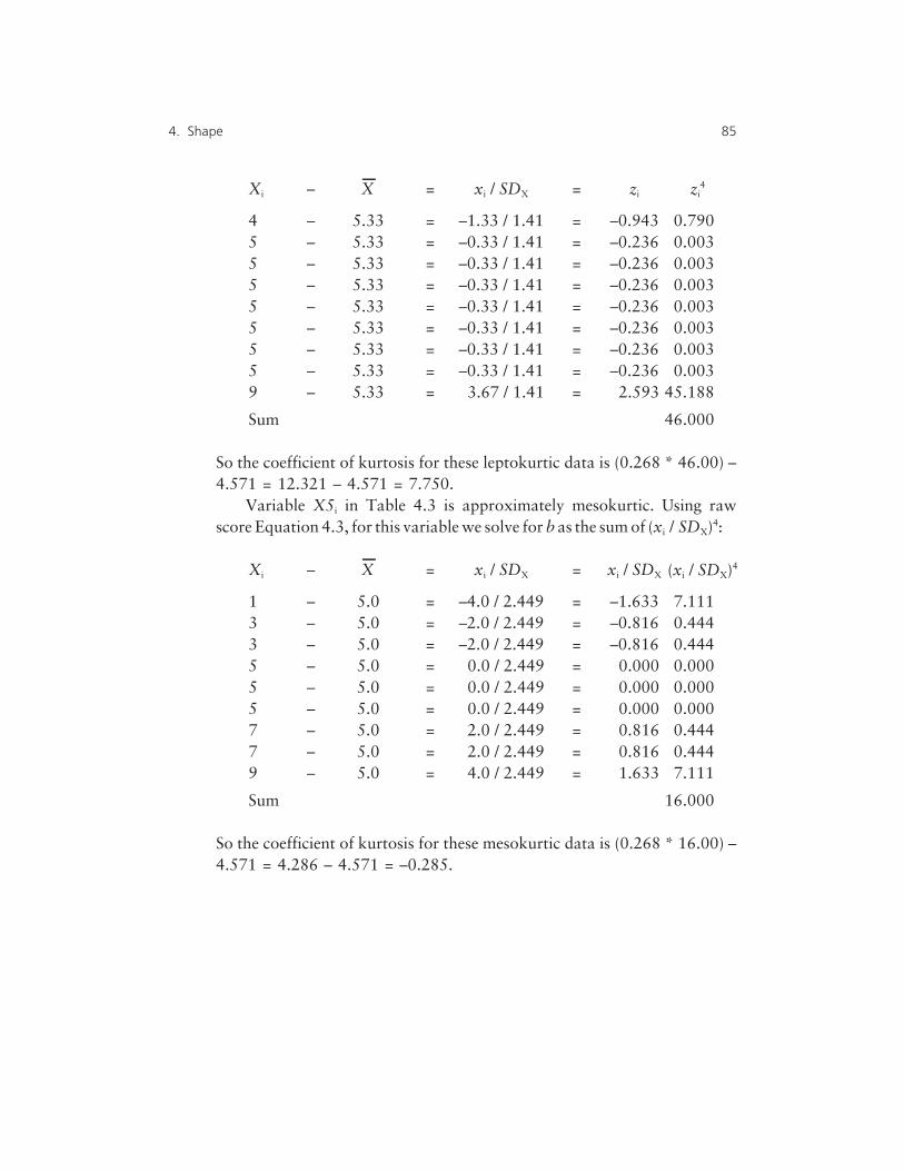
Xi – X = xi / SDX = zi zi4

4 – 5.33 = –1.33 / 1.41 = –0.943 0.7905 – 5.33 = –0.33 / 1.41 = –0.236 0.0035 – 5.33 = –0.33 / 1.41 = –0.236 0.0035 – 5.33 = –0.33 / 1.41 = –0.236 0.0035 – 5.33 = –0.33 / 1.41 = –0.236 0.0035 – 5.33 = –0.33 / 1.41 = –0.236 0.0035 – 5.33 = –0.33 / 1.41 = –0.236 0.0035 – 5.33 = –0.33 / 1.41 = –0.236 0.0039 – 5.33 = 3.67 / 1.41 = 2.593 45.188

Sum 46.000

So the coefficient of kurtosis for these leptokurtic data is (0.268 * 46.00) –4.571 = 12.321 – 4.571 = 7.750.

Variable X5i in Table 4.3 is approximately mesokurtic. Using rawscore Equation 4.3, for this variable we solve for b as the sum of (xi / SDX)4:

Xi – X = xi / SDX = xi / SDX

1 – 5.0 = –4.0 / 2.449 = –1.633 7.1113 – 5.0 = –2.0 / 2.449 = –0.816 0.4443 – 5.0 = –2.0 / 2.449 = –0.816 0.4445 – 5.0 = 0.0 / 2.449 = 0.000 0.0005 – 5.0 = 0.0 / 2.449 = 0.000 0.0005 – 5.0 = 0.0 / 2.449 = 0.000 0.0007 – 5.0 = 2.0 / 2.449 = 0.816 0.4447 – 5.0 = 2.0 / 2.449 = 0.816 0.4449 – 5.0 = 4.0 / 2.449 = 1.633 7.111

Sum 16.000

So the coefficient of kurtosis for these mesokurtic data is (0.268 * 16.00) –4.571 = 4.286 – 4.571 = –0.285.

4. Shape 85

(xi / SDX)4

�� Normal Distributions

Judgments of symmetry are rather straightforward and require no arbi-trary benchmark. We can judge quite well when people (or data) are sym-metrical without invoking a standard. But how can height relative towidth of a blind date candidate be evaluated without a standard for howmuch of the person (or data) should be in the extremes, and how muchshould be in the middle?

In conventional blind-date negotiations, one invariably turns to astandard (e.g., “She is shaped like Marilyn Monroe” or “He is shaped likeClark Gable” [younger readers may wish to substitute Brad Pitt, ParisHilton, or some other choice, as a standard]). So, too, there is a standardin evaluating when data are Goldilocks just right, or mesokurtic, in thedistribution of height relative to width.

Normal distributions are used as the gold standard for evaluatingkurtosis (Henson, 1999). There are infinitely many different normal distri-butions. Every normal distribution is perfectly mesokurtic (i.e., has a coef-ficient of kurtosis of exactly zero).

Normal distributions were conceptualized by de Moivre, later used byLaplace, and popularized by Gauss in 1809 in the analysis of astronomicaldata. Normal distributions have many very important uses in statistics.Consequently, these distributions are given several synonymous names,for reasons that by now are evident to the reader. The synonymous namesinclude “normal distributions,” “Gaussian distributions,” and somewhatcolloquially, “bell-shaped distributions.”

There is only one normal distribution for a given combination of Mand SD. However, there are infinitely many normal distributions, becausethere are infinitely many values of M and SD. Of course, two differentnormal distributions may have (a) different means but the same SDs,(b) the same means but different SDs, or (c) both different means and dif-ferent SDs.

For a given score on Xi, the height of the histogram can be determinedusing the equation

u = [1 / (SD)((2(pi))0.5)][e–{((Xi–M)(Xi–M)) / (2(SD)(SD))}] (4.8)


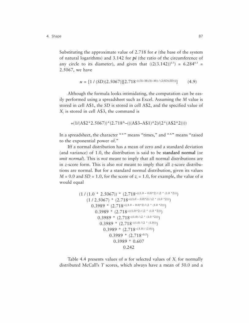
Substituting the approximate value of 2.718 for e (the base of the systemof natural logarithms) and 3.142 for pi (the ratio of the circumference ofany circle to its diameter), and given that ((2(3.142))0.5) = 6.2840.5 =2.5067, we have

u = [1 / (SD)(2.5067)][2.718–{((Xi–M)(Xi–M)) / (2(SD)(SD))}] (4.9)

Although the formula looks intimidating, the computation can be eas-ily performed using a spreadsheet such as Excel. Assuming the M value isstored in cell A$1, the SD is stored in cell A$2, and the specified value ofXi is stored in cell A$3, the command is

+(1/(A$2*2.5067))*(2.718^–(((A$3–A$1)^2)/(2*(A$2^2))))

In a spreadsheet, the character “*” means “times,” and “^” means “raisedto the exponential power of.”

Iff a normal distribution has a mean of zero and a standard deviation(and variance) of 1.0, the distribution is said to be standard normal (orunit normal). This is not meant to imply that all normal distributions arein z-score form. This is also not meant to imply that all z-score distribu-tions are normal. But for a standard normal distribution, given its valuesM = 0.0 and SD = 1.0, for the score of zi = 1.0, for example, the value of uwould equal

(1 / (1.0 * 2.5067)) * (2.718–(((1.0 – 0.0)^2) / (2 * (1.0 ^2))))(1 / 2.5067) * (2.718–(((1.0 – 0.0)^2) / (2 * (1.0 ^2))))

0.3989 * (2.718–(((1.0 – 0.0)^2) / (2 * (1.0 ^2))))0.3989 * (2.718–(((1.0)^2) / (2 * (1.0 ^2))))

0.3989 * (2.718–((1.0) / (2 * (1.0 ^2))))0.3989 * (2.718–((1.0) / (2 * (1.0))))

0.3989 * (2.718–((1.0) / (2.0)))0.3989 * (2.718–0.5)

0.3989 * 0.6070.242

Table 4.4 presents values of u for selected values of Xi for normallydistributed McCall’s T scores, which always have a mean of 50.0 and a

4. Shape 87

standard deviation of 10.0. Figure 4.4 is an SPSS graphic of a plot of val-ues of u against corresponding values of Xi, which displays as a bell shape.

All normal distributions have certain properties. First, normal distri-butions are symmetric and unimodal, with mode = Mdn = M. Second, nor-


TABLE 4.4. Values of u for 61 Values of Xi for aNormal Distribution When M = 50 and SD = 10

Xi u Xi u Xi u

20 0.0004 40 0.0242 60 0.024221 0.0006 41 0.0266 61 0.021822 0.0008 42 0.0290 62 0.019423 0.0010 43 0.0312 63 0.017124 0.0014 44 0.0333 64 0.015025 0.0018 45 0.0352 65 0.013026 0.0022 46 0.0368 66 0.011127 0.0028 47 0.0381 67 0.009428 0.0035 48 0.0391 68 0.007929 0.0044 49 0.0397 69 0.006630 0.0054 50 0.0399 70 0.005431 0.0066 51 0.0397 71 0.004432 0.0079 52 0.0391 72 0.003533 0.0094 53 0.0381 73 0.002834 0.0111 54 0.0368 74 0.002235 0.0130 55 0.0352 75 0.001836 0.0150 56 0.0333 76 0.001437 0.0171 57 0.0312 77 0.001038 0.0194 58 0.0290 78 0.000839 0.0218 59 0.0266 79 0.0006

80 0.0004

FIGURE 4.4. Normal distribution for M = 50.0 and SD = 10.0

mal distributions are asymptotic to the horizontal (i.e., X) axis, whichmeans that the further scores are from the mean, the more their frequen-cies decrease, but the frequencies never reach zero.

The asymptotic properties of the normal distribution can be con-cretely understood if we determine the proportion (or, if multiplied by100, the percentage) of datapoints below a given score, Xi, in a given nor-mal distribution. The spreadsheet Excel will return this value if we invokethe statistical function:

=normdist(X,M,SD,true)

where X is the given score, M is the mean of the normal distribution ofinterest, and SD is the standard deviation of the normal distribution ofinterest.

For example, if we presume that IQ scores are exactly normally dis-tributed and if we input

=NORMDIST(175,100,15,TRUE)

Excel will return the value

0.999999713

This means that 99.9999713% of all people have an IQ score less than175. But, by the same token, 0.0000287% of all people (or roughly 287people out of a billion) have an IQ of 175 or more. Asymptotic in this con-text means, at least theoretically, that there is (or eventually will be)always somebody smarter out there!

The normal distribution has the interesting property that fixed pro-portions of scores are in the six regions defined by the mean plus or minuszero, one, two, or three times the standard deviation. For our IQ scoreexample, we obtain

M Multiplier SD IQ % below

100.0 –3 15.0 55 00.135100.0 –2 15.0 70 02.275

4. Shape 89

100.0 –1 15.0 85 15.866100.0 0 15.0 100 50.000100.0 1 15.0 115 84.134100.0 2 15.0 130 97.725100.0 3 15.0 145 99.865

Fixed percentages (or proportions) of scores fall between these bound-aries. For example, 68.27% (84.134 – 15.866) of the scores fall betweenM – 1(SD) and M + 1(SD), and 95.45% of the scores fall betweenM – 2(SD) and M + 2(SD). The percentage of additional scores capturedby going out successive multipliers of the SD can also be computed (e.g.,68.27% – 0.0% = 68.27%; 95.45% – 68.27% = 27.18%; 99.73% –95.45% = 4.28%). So we have for each and every one of the infinitelymany normal distributions

Unique to oneCumulative more SD in

Region % in region both directions

M – 1(SD) to M + 1(SD) 68.27 68.27%M – 2(SD) to M + 2(SD) 95.45 27.18%M – 3(SD) to M + 3(SD) 99.73 4.28%

By the same token, because all normal distributions are symmetric,34.13% (68.27% / 2) of the scores fall specifically in the region fromM – 1(SD) to M, and 34.13% of the scores fall in the region fromM + 1(SD) to M. Similarly, 13.59% (27.18% / 2) of the scores fall specifi-cally in the region from M – 2(SD) to M – 1(SD), and 13.59% of thescores fall in the region from M + 1(SD) to M to M + 2(SD) to M. So wehave, for the six regions consuming 99.73% of scores, for each and everyone of the infinitely many normal distributions,

Region % in region

<M – 3(SD) 0.135M – 3(SD) to M – 2(SD) 2.14M – 2(SD) to M – 1(SD) 13.59M – 1(SD) to M – 0(SD) 34.13


M – 0(SD) to M + 1(SD) 34.13M – 1(SD) to M + 2(SD) 13.59M – 2(SD) to M + 3(SD) 2.14

>M + 3(SD) 0.135

Knowledge of these relationships is useful because intervally-scaleddata, at least when collected on large numbers of participants, tend to benormally-distributed. Thus, these percentages tend to be approximatelyaccurate in many research situations.

If I give an examination to a huge number of doctoral students, andthe data are normally distributed, with M = 15.0 and SD = 3.0, I cananswer such questions as these:

1. What percentage of students had a score less than 21.0?[Answer: 50.0% + 34.13 + 13.59% = 97.72%]

2. What is the score below which 15.865% of the students score?[Answer: 15.0]

3. What percentage of students score between 12.0 and 21.0?[Answer: 34.13% + 34.13% + 13.59% = 81.85%]

Indeed, if we employ the Excel NORMDIST statistical function, we candetermine the percentages for any score, or the score for any multiple(including noninteger multiples) of the standard deviation.

�� Two Additional Univariate Graphics

As noted in Chapter 2, histograms are a useful univariate graphic. Histo-grams provide insight about score location, dispersion, and shape. Histo-grams can be readily obtained in SPSS by using the HISTOGRAM procedureunder the GRAPHS menu. And as an option, SPSS will draw a normal curveover the histogram for comparative purposes.

Another useful univariate graphic is the stem-and-leaf plot. Theseplots can be produced in SPSS using the EXAMINE procedure under theSUMMARIZE submenu in the ANALYZE menu. Assume we have 34 scores: {1,10, 10, 11, 12, 12, 13, 14, 14, 15, 16, 16, 17, 18, 18, 19, 20, 20, 21, 22,

4. Shape 91

22, 23, 24, 24, 25, 26, 26, 27, 28, 28, 29, 30, 30, 45}. Figure 4.5 presentsa stem-and-leaf plot for these data.

The “stem” of the stem-and-leaf plot is the leading digit of the num-bers (i.e., here 0, 1, 2, 3, or 4). The “leaf” is the next digit defining a givendatapoint. For example, the Figure 4.5 plot indicates that one person hada score with a stem of 0 and a leaf of 1 (i.e., one person had a score of 01).Eight people had the stem of 1, and two of these eight people had leafs of0 (i.e., scores of 10). One of these eight people had a leaf of 1 (i.e., a scoreof 11). Two of these eight people had leafs of 2 (i.e., scores of 12). Oneperson had a score labeled “extreme” (i.e., 45).

A third, wonderful univariate graphic is the box plot (or the box-and-whiskers plot). The SPSS EXAMINE procedure will also produce this plot.Figure 4.6 presents the box plot for these data.

The initial step in creating the box plot is to compute the median loca-tion, truncating any fractional values. For n = 34, the median location is(n + 1) / 2 = (34 + 1) / 2 = 35 / 2 = 17.5, which we truncate to 17. Themedian itself for these data is 20.0. The dark horizontal line within thevertical box plot is drawn at MdnX.

We next compute hinge locations, which equal (median location + 1) / 2.For our data, we have (17 + 1) / 2 = 18 / 2 = 9. We use this to find thehinges, which here are the scores located ninth from the bottom (i.e., 14)and ninth from the top (i.e., 26). For our data, the hinges are 14.0 and26.0.

For large samples, the hinges correspond to the first and third quartilescores, and will be near these scores for small samples. Thus, some com-puter programs create the box plot using Q1 and Q3 (i.e., the 25th and the75th percentiles, using Equation 2.1) rather than the hinges.

Next, we compute the hinge spread, which is simply the rangebetween the two hinges (i.e., here 26.0 – 14.0 = 12.0) and either equals orapproximates the IQRX. We then use the hinge spread to compute theinner fences that we will use as boundaries for identifying outlying scores.The lower inner fence equals the lower hinge (here 14.0) minus the con-stant of 1.5 times the hinge spread (i.e., 14.0 – 1.5(12.0) = 14.0 – 18.0 =–6.0). The upper inner fence equals the upper hinge (here 26.0) plus theconstant of 1.5 times the hinge spread (i.e., 26.0 + 1.5(12.0) = 26.0 + 18.0= 44.0).

Finally, we compute the adjacent values by comparing our actual


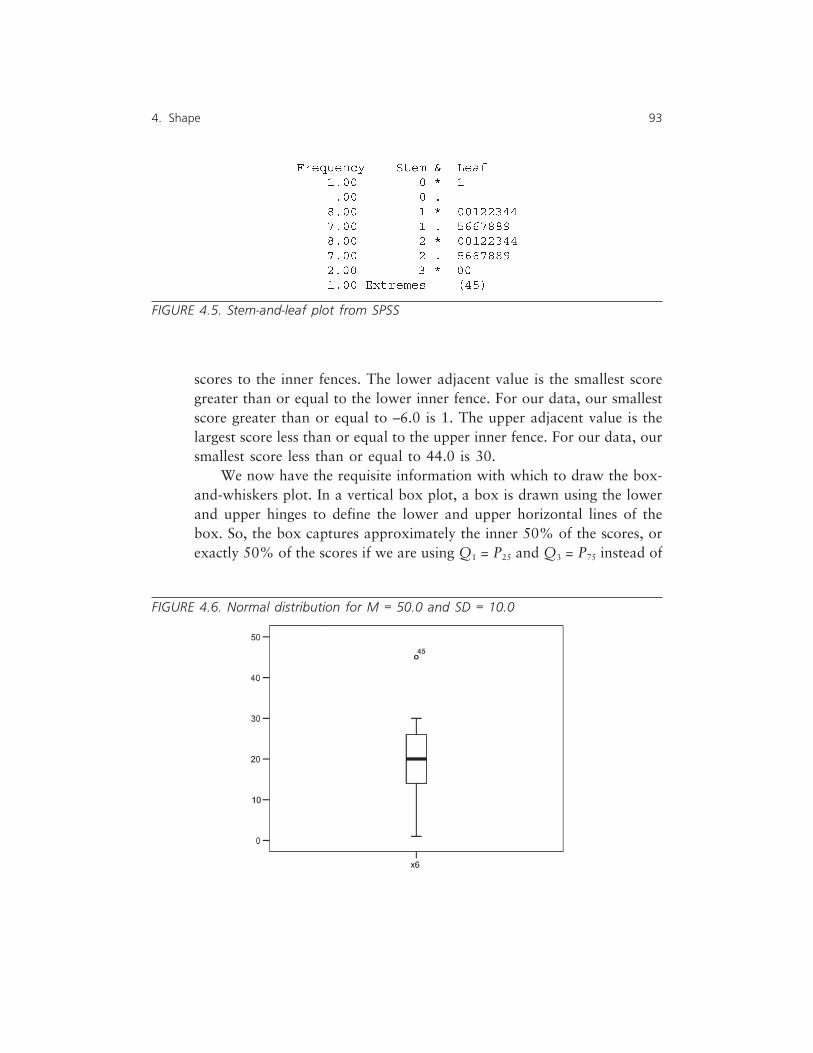
scores to the inner fences. The lower adjacent value is the smallest scoregreater than or equal to the lower inner fence. For our data, our smallestscore greater than or equal to –6.0 is 1. The upper adjacent value is thelargest score less than or equal to the upper inner fence. For our data, oursmallest score less than or equal to 44.0 is 30.

We now have the requisite information with which to draw the box-and-whiskers plot. In a vertical box plot, a box is drawn using the lowerand upper hinges to define the lower and upper horizontal lines of thebox. So, the box captures approximately the inner 50% of the scores, orexactly 50% of the scores if we are using Q1 = P25 and Q3 = P75 instead of

4. Shape 93

FIGURE 4.5. Stem-and-leaf plot from SPSS

FIGURE 4.6. Normal distribution for M = 50.0 and SD = 10.0

hinges. A dark horizontal line is drawn within the box to represent themedian.

A “whisker” is drawn off the bottom of the vertical box down to thelower adjacent fence value (i.e., 1). A whisker is also drawn off the top ofthe vertical box up to the upper adjacent fence value (i.e., 30).

Any scores below the lower adjacent fence are portrayed as asterisks(or circles) within our plot. Here we have no scores below our lower adja-cent fence of 1. Any scores above the upper adjacent fence are also por-trayed as asterisks (or circles). We have one score (i.e., 45) above theupper adjacent fence of 30.

The box plot tells us a good deal about our data. If the data areapproximately symmetrical, the median will be about halfway between thesmallest and the largest scores and roughly in the middle of the box, andthe whiskers will be of roughly equal length.

Box plots are also useful in identifying potential outlying scores, asregards location, dispersion, and shape. The plots also give an impressionof just how extreme outlying scores may be. Of course, an outlier on onevariable may not be outlying on any other variables. And, as we shall seein Chapter 5, an outlier as regards location, dispersion, and shape may notbe an outlier on descriptions of relationships among the variables.

Some Key Concepts

The shapes of data distributions that are at least intervally-scaled maybe characterized by computing statistics that quantify (a) symmetry(i.e., the coefficient of skewness) and (b) height relative to width (i.e.,the coefficient of kurtosis). Kurtosis evaluates shape against the stan-dard of the normal curve, which has a coefficient of skewness of zeroand a coefficient of kurtosis of zero.

There are infinitely many normal distributions. But for data withboth (a) a given mean and (b) a given SD, only one normal distribu-tion exists. Iff the data are in z-score form, the normal distribution iscalled “standard normal.” Distributions may be standard, normal, orboth. Symmetry may be established visually by examining histogramsof the data, but the normality of symmetrical data cannot be estab-lished merely by examining histograms.

When data that are at least intervally-scaled are collected withlarge samples, often the data are normal or near normal. In such caseswe can invoke knowledge of what percentages of scores fall within


score ranges in the normal distribution in order to more fully under-stand the dynamics within our data.


1. If we are given the score range for a normal distribution, how can we use

only this information to solve for the approximate SD of the scores?

2. For a given dataset, how will using mean substitution for missing values

impact the coefficient of skewness for data that were initially skewed?

How will using mean substitution for missing values impact the coeffi-

cient of kurtosis? How does mean substitution differentially impact

postsubstitution means, SD, skewness, and kurtosis?

3. Draw a distribution for which MX < MdnX, but modeX > MX and modeX >

MdnX. Draw a distribution for which MX > MdnX, but modeX < MX and

modeX < MdnX.

4. The scores presented in the Appendix are nearly normally distributed.

Enter these z scores into SPSS. Then click on ANALYZE, then on DESCRIPTIVE

STATISTICS, and then on FREQUENCIES. Use the STATISTICS subcommand to

obtain the score mean, median, SD, and coefficients of skewness and

kurtosis. Also, graph the scores by using the CHARTS subcommand; select

HISTOGRAM and check WITH NORMAL CURVE. After the chart is generated,

double left click on the chart to enter the CHART EDITOR. Click on EDIT, then

SELECT X AXIS, and set the X-axis minimum value to –5 and the maximum

value to 55. This allows comparisons of graphs with different data

because the X axis will be scaled consistently.

Now use the command

COMPUTE x2 = (z * 4) + 20 .

to create another set of scores. Compute the same statistics for these

data, and plot the scores. How do the skewness and kurtosis coefficients

of the two sets of scores compare? How well does each histogram fit the

respective normal curve plot? What does this imply about whether there

is only one normal distribution?

4. Shape 95

5. Using the data and additive and multiplicative constants in Reflection

Problem #3 in Chapter 2, what rule can we formulate to express the

effects on coefficients of skewness and kurtosis of additive constants?

What rule can we formulate to express the effects on coefficients of

skewness and kurtosis of multiplicative constants? When will a multiplica-

tive constant not change the value of the original coefficient of skew-

ness? When will a multiplicative constant change the value of the original

coefficient of skewness?


5

BivariateRelationships

The descriptive statistics explained in Chapters 2 through 4 areunivariate statistics. That is, these descriptions can be formulatedto characterize data even when only one variable is present.

However, real science is always about the investigation of rela-tionships that occur under stated conditions. Though we can describe fea-tures of data even if we only have data on a single variable, and suchunivariate descriptions may hold some personal interest for us or satisfyour curiosity, only when we have at least two variables do things really getserious.

In the simplest case of true science, we have exactly two variables. Thestatistics that describe relationships between two variables are bivariatestatistics. We can only compute these statistics when we have two vari-ables.

But the bivariate relationship descriptive statistics discussed here,although important in and of themselves, are also critical in laying theconceptual foundation for understanding the sophisticated analyses thataccommodate even more than two variables. Indeed, even very compli-

97

cated multivariate statistics can be explained using bivariate statistics con-cepts (Fan, 1996; Kimbell, 2001; Thompson, 1991a).

Parametric statistics presume that the dependent variable is intervally-scaled, and make shape assumptions as well. An important theme of thisbook, which we are building toward, is that all statistical analyses are cor-relational and are part of a global general linear model (Bagozzi, Fornell,& Larcker, 1981; Cohen, 1968; Knapp, 1978). The general linear model(GLM) has important implications for how we conduct and interpretquantitative analyses.

Of course, just as levels of scale drive what descriptive statistics can becomputed for univariate characterizations, levels of scale also impactoptions in the bivariate case. However, now the levels of scale of two vari-ables must be simultaneously considered.

We will emphasize four combinations of scale: (a) the Pearson r,which requires that both variables are at least intervally-scaled;(b) Spearman’s rho (ρ), which requires that both variables are at leastordinally-scaled (but one or both variables may be scaled higher);(c) phi (φ), which can be used with two variables that are dichotomous;and (d) point–biserial correlation (rpb), which is used when one variableis dichotomously scored and the other variable is at least intervally-scaled.

Additional descriptive relationship statistics (e.g., biserial andtetrachoric correlation, Kendall’s tau (τ)) are beyond the scope of the pres-ent treatment, but the four coefficients listed in the previous paragraphwill stand you in good stead in commonly-encountered research situa-tions.

These four coefficients are all score-world descriptive statistics. Fur-thermore, φ and rpb are merely algebraically-equivalent formulas that canbe used in place of an explicitly Pearson r formula, but yield exactly thesame result as a Pearson r computation, and so are the Pearson r for cer-tain levels-of-scale combinations. And Spearman’s ρ is merely the Pearsonr (or an algebraic equivalent) applied to data either expressed originally asranks, or data converted to ranks.


�� Pearson’s r

When both variables are at least intervally-scaled, we can compute thePearson product–moment correlation coefficient (r) as

rXY = COVXY / (SDX * SDY) (5.1)

where COVXY is also a description of bivariate relationship, called thecovariance, and which is computed for a sample as

COVXY = (Σ(Xi – MX)(Yi – MY)) / (n – 1) (5.2)

The standard deviations are computed using the statistic formula thatassumes we have sample data. Equation 5.2 for the COVXY invokes devia-tion scores, as do the first, second, and third moment about the mean, andcan be reexpressed as

COVXY = (Σ(xi[yi])) / (n – 1) (5.3)

The fact that the numerator of the COVXY uses deviation scores sug-gests the possibility of using z scores in an algebraically equivalent for-mula, because all z scores are themselves deviation scores (thus thelowercase z). And Equation 5.1, given z scores, because both standarddeviations equal 1.0, simplifies to rzXzY = COVzXzY. For a given dataset, rXY

always exactly equals rzXzY (for reasons that we will encounter later). So wecan also compute the Pearson r for either the X with the Y scores or the zX

with the zY scores (or the zX with the Y scores, or the X with the zY scores)as

rXY = (Σ(zXi[zYi])) / (n – 1) (5.4)

Equation 5.1 makes obvious that the Pearson r is a standardizedcovariance (i.e., a covariance with the standard deviations removed bydivision), and that r is not only in the score world, but also is specificallyin the standardized score world. Equation 5.4 makes even more apparent

5. Bivariate Relationships 99

the fact that r is a standardized, score-world descriptive statistic. TheCOVXY, on the other hand, is an area-world descriptive statistic.

Given that the covariance is a description of bivariate relationship,also requiring interval scaling of both variables, why is COVXY not itselfused as a description of bivariate association? To answer this question,first we look at an algebraic rearrangement of Equation 5.1:

COVXY = rXY * SDX * SDY (5.5)

where “*” means “multiplied by.”This formula asserts that three factors influence the covariance as a

descriptive result, and thus makes the description confounded and ambig-uous, at least in some cases. We can see this in the following data for pairsof variables, all of which have COVXY approximately equal to 10,000:

COVXY = rXY * SDX * SDY

10000.0 = 1.00 * 100.00 * 100.0010000.1 = 0.75 * 0.25 * 53334.0010000.0 = 0.50 * 100.00 * 200.0010000.0 = 0.25 * 1.00 * 40000.0010000.0 = 0.01 * 100.00 * 10000.0010000.0 = 0.01 * 0.50 * 2000000.00

Thus, the covariance is of limited descriptive value, because a given resultmay reflect a lot of relationship and little score spread on either variable,or a little relationship and a lot of score dispersion on one or both vari-ables, or many other possibilities!

This is not meant to suggest that the covariance is unimportant forother purposes not involving description. The covariance is important inits own right as part of the computation of r. And the covariance is alsoused as the primary basis for many multivariate analyses (i.e., analysessimultaneously considering multiple dependent variables, an importanttopic, but one not covered in this book).

Several things are made obvious by thinking about Equation 5.1.First, r is a bivariate statistic. It is truly excellent that r cannot be com-puted unless both X and Y are variables. If either or both X and Y are con-stants, r is undefined, because division by zero is impermissible. Having r


be undefined unless there are two variables is fantastic, because this meanswe don’t have to hire statistics police to monitor all statistics calculationsthroughout the world to make sure that no one is computing r unless bothX and Y are variables.

Remember that

undefined ≠ 0 (5.6)

Two variables may have a correlation of zero. But having an undefinedr does not (i.e., not) mean that the correlation is zero. If you know that anr = 0, you know certainly that both X and Y must have been variables, orthere simply would be no r.

If we think further about Equation 5.1, rather than rotely memorizingthe equation, we can extrapolate additional revelations (i.e., the intellec-tual orgasms that learning is really all about). First, because the two SDscan never be negative, rXY and the COVXY always have the same sign. Sec-ond, rXY and COVXY will always be equal if (but not iff) the two standarddeviations have a crossproduct of 1.0, which will occur iff the two SDs arereciprocals of each other (e.g., SDX = 1.0, SDY = 1.0; SDX = 0.5, SDY =2.0). Third, rXY and the COVXY will always be equal (and zero) if (but notiff) either the rXY or the COVXY is zero, regardless of the standard devia-tions, as long as both X and Y are variables (i.e., SDX ≠ 0 and SDY ≠ 0).

�� Three Features of r

r Describes Only Linear Relationship

A scattergram (or scatterplot) is a bivariate graphic displaying the pairs ofscores for each individual in the dataset. Just as a histogram is ubiquitousin the univariate case, the scattergram is ubiquitous in bivariate statistics.

Table 5.1 presents the scores of 12 people on the variables X and Y.Figure 5.1 presents the scattergram of these data. As is the case in a histo-gram, unless otherwise declared in a figure note, each asterisk (or diamondor square or other object) represents one person. But in a scattergram,each asterisk (diamond, or other object) represents two scores for a givenperson, rather than only one score. For example, in the Figure 5.1 scatter-


gram, note that Paul is the lowest, leftmost asterisk, and Patty is the high-est, rightmost asterisk. Paul’s asterisk communicates that his X and Yscores were 1 and 1, respectively.

One way to conceptualize r is to think of r as addressing the question“How well does the line of best possible fit capture the asterisks in the


FIGURE 5.1. Scattergram of the Table 5.1 data

TABLE 5.1. Scores of n = 12 Participants on Two Variables

Participant/statistic Xi Yi xi yi xyi

Paul 1 1 –3.0 –4.5 13.5Christopher 2 2 –2.0 –3.5 7.0Michael 3 3 –1.0 –2.5 2.5Ralph 5 5 1.0 –0.5 –0.5Randy 6 6 2.0 0.5 1.0Steve 7 7 3.0 1.5 4.5Jennifer 1 4 –3.0 –1.5 4.5Stephanie 2 5 –2.0 –0.5 1.0Elizabeth 3 6 –1.0 0.5 –0.5Sarah 5 8 1.0 2.5 2.5Judy 6 9 2.0 3.5 7.0Patty 7 10 3.0 4.5 13.5

Sum 48.00 66.00 0.00 0.00 56.00M 4.00 5.50 0.00 0.00SD 2.26 2.75

Note. Selected entries for the five people who scored below the means on both variables arepresented in bold. Selected entries for the five people who scored above the means on bothvariables are presented in italics.

scattergram?” The line of best fit has been drawn in Figure 5.1 for theTable 5.1 data.

The Pearson r will be at its minimum or maximum limits (–1 or +1,respectively) iff all the asterisks in the scattergram are on the line. An r of+1 or –1 is called a perfect relationship. When there is no linear relation-ship between the two variables, any line of best fit that we draw will cap-ture the asterisks equally badly, and r will equal zero.

When r is positive, the relationship between the two variables is saidto be direct or positive. When the linear relationship is positive, as scoreson one variable become larger, scores on the other variable tend to also belarger (or the converse; i.e., scores on both variables tend to get smallertogether). For example, the number of calories people consume on averageeach day tends to be directly related to their weights.

When the linear relationship (and Pearson’s r) is negative, as scores onone variable become larger, scores on the other variable tend to be smaller(or vice versa). For example, the number of miles people jog each daytends to be inversely related to their weights.

In the unstandardized score world, the line of best fit is a function ofY , X , SDY, SDX, and rXY. The line of best fit will be horizontal (flat) iff r iszero, and otherwise will not be flat.

Table 5.1 presents the means and standard deviations of the two vari-ables, computed in the manner explained in previous chapters. Let’s nowsolve for the Pearson product–moment correlation coefficient. For thesedata, as reported in Table 5.1, the sum of the 12 crossproducts (i.e.,Σxi[yi]) is 56.00, which according to Equation 5.3 yields a COVXY of 5.09(i.e., 56.00 / 11). Thus, rXY for these data is COVXY / [(SDX)(SDY)] = 5.09 /[(2.26)(2.75)] = 5.09 / 6.22 = 0.82.

Now, how do we know where to draw the line of best fit within thescattergram? We can identify (fix) the location of a line as long as we cansolve for any two points on the line.

An important implication of Equation 5.2 is that the intercept of thetwo means is always on the line of best fit. Indeed, the line of best fitalways pivots on this point. In fact, this point is so important that ratherthan call this point the Cartesian coordinate of the two means, we insteadcall this location the centroid. (If we called the point defined by the meansof all the measured variables “the means of all the measured variables,”everybody would know what we were talking about, and that would beunsatisfactory.)


So one point defining our line of best fit for our data is the location,4.00 on X, and 5.50 on Y. We can solve for a second point on the line ofbest fit, if we know the Pearson correlation coefficient (here rXY = 0.82).The point where the line of best fit crosses the Y (or vertical axis; i.e., Ywhen X = 0) is called a.

We can solve for a as

a = Y – [rXY(SDY / SDX)](X) (5.7)

For our data we have a as

5.50 – [0.82(2.75 / 2.26)](4.00)5.50 – [0.82(1.22)](4.00)

5.50 – [1.00](4.00)5.50 – 4.00

1.50

Notice that the line of best fit does not capture any of the asterisks inthe Figure 5.1 scattergram. Note also that r does not ask “how many”asterisks we can catch with a line, but instead focuses on “how close” wecan come to capturing the asterisks, under a restriction that we cannotfocus exclusively on some asterisks (e.g., the top six asterisks in the scat-tergram) unfairly at the expense of any other asterisks.

I want to emphasize that r measures linear, and only linear, relation-ship, because we are trying to catch all the asterisks with a line. However,never forget that curvilinear (i.e., nonlinear) relationships are also entirelypossible. Consider the data in Table 5.2 for George, which involve mea-suring how much pleasure he experiences upon being given daily variousamounts of vanilla ice cream.

George is what statisticians call “a vanilla ice-cream hound.” GeorgeLOVES ice cream. George would eat a shoe if the shoe had ice cream on it.But in this case, as in many others, at some point you can get too mucheven of a good thing (e.g., teacher praise of first-grade students) or even avery good thing (e.g., use your imagination).

A hypothetical “pleasure-ometer” is used to measure how much joy


or, conversely, unhappiness George experiences. On this pleasure-ometer,the maximum pleasure a human can experience yields a score of +10. Themaximum unhappiness a human can experience yields a score of –10.

The Pearson r for the Table 5.2 data is 0.00. There is no linear rela-tionship between these data. However, if we examine the Figure 5.2 plotof the Table 5.2 data, it becomes obvious that there is a systematic and,indeed, virtually perfect relationship between these variables. The relation-ship, however, is curvilinear.

When given successively more vanilla ice cream each day, from 1 to 5gallons, George’s pleasure increases each time. However, the incremental


TABLE 5.2. Pleasure-ometer Readings forGeorge over 10 Days of Ice Cream Deliveries

Day Gallons delivered Pleasure

1 1 12 2 43 3 74 4 95 5 106 6 107 7 98 8 79 9 4

10 10 1

FIGURE 5.2. Scattergram of the Table 5.2 data

increase in his pleasure decreases with each successive increment in icecream. There is no difference in pleasure experienced when moving from5 to 6 gallons. And every increase in ice cream from 6 to 10 gallons causesa reduction in pleasure.

Indeed, Figure 5.2 suggests that going from 10 to 11 and then to 12gallons of ice cream actually causes unhappiness, even for an ice-creamhound! The projected pleasure-ometer readings for these amounts of icecream would be –3.7 and –9.2.

The Pearson r for these data is zero even though there is a near-perfectcurvilinear relationship between the variables, because the Pearson r onlymeasures linear relationship. This means that when r = 0.0, there may beanywhere from a zero relationship of all kinds (including curvilinear) to aperfect relationship of all kinds (including curvilinear).

The only time that r tells us both (a) about linear relationship and (b)that there is zero curvilinear relationship is when r is perfect (either –1 or+1). The reason is that when there is a perfect linear relationship, there isno possibility of any curvilinear relationship. If all the asterisks define andare on a line in the scattergram, no curvilinear pattern is possible.

Relationships between variables are often either partially or primarilylinear, although variables often also have elements of curvilinear relation-ship at some point. Thus curvilinear relationships, as well as linear rela-tionships, are of interest in research.

There are two ways to investigate curvilinear relationship. First,graphics like the scattergram can be used to inform judgment aboutcurvilinear relationship. Second, some descriptive statistics that we willencounter in subsequent chapters can be used to quantify the amount ofcurvilinear relationship.

r Is in an Ordinal Metric

The Pearson r is a descriptive statistic quantifying the amount of linearrelationship between two variables that are at least intervally-scaled.However, this does not mean that the r statistic itself is intervally-scaled.

In fact, r itself is ordinally-scaled as regards the variance common tothe two variables. This means that rAB = +1.0 is larger than rXY = +0.5 or


that rAB = +1.0 in one sample is larger than rAB = +0.5 in a separate sample.However, the r of +1.0 is not twice as large as the r of +0.5. Two trans-forms of Pearson r are fairly common, although they are typically done fordifferent purposes.

Fisher’s r-to-z Transform

One way of reexpressing r is to invoke a transformation, called the r-to-ztransformation, developed by Sir Ronald Fisher. Fisher developed a num-ber of statistical methods, for which he was knighted in Great Britain (wewill hear more about him in Chapter 10, when we discuss the analysis ofvariance). This transform was developed for statistical purposes such ashypothesis testing, a topic covered in Chapter 6.

The r-to-z transform yields a score-world statistic. The formula forFisher’s r-to-z transformation is

0.5 * (LN((1 + ABS(r)) / (1 – ABS(r)))) (5.8)

where LN means “take the natural logarithm of” and ABS means “takethe absolute value of.” After the computation, if r was negative, the nega-tive sign is restored to the r-to-z value. This formula can be easily executedin Excel, presuming that the r value has been inserted into spreadsheet cellA1, using the following command:

=.5*(@ln((1+@abs(A1))/(1-@abs(A1))))

For example, for r = 0.82, we obtain

= 0.5(LN((1 + 0.82) / (1 – 0.82)))= 0.5(LN((1.82) / (0.18)))

= 0.5(LN(10.11))= 0.5(2.31)

= 1.16


As another example, consider the extreme value of r = 0.99. Now wehave

= 0.5(LN((1 + 0.99) / (1 – 0.99)))= 0.5(LN((1.99) / (0.01)))

= 0.5(LN(199.00))= 0.5(5.29)

= 2.65

Note that the r-to-z transform, not unlike the z scores in a normal distribu-tion, tends to range between roughly –3 and +3.

r2 as a Descriptive Statistic

The squared value of r (r2), unlike r, is itself intervally-scaled as regards thevariance common to the two variables. Thus, rAB

2 = +1.0 (or 100%) is fourtimes larger than rXY

2 = +0.25 (or 25%). And the result also means thatrAB = +1.0 is four times larger than rXY = +0.5.

The descriptive statistic r2 is called the coefficient of determination orthe common variance. Of course, unlike r, which is in the standardizedscore world, r2 is in the area world. The interval properties of r2 have ledto the popular (albeit extremely brief) hit rap song, the only lyrics ofwhich are “Square, before you compare!”

Table 5.3 presents some interesting uses of the coefficient of determi-nation in comparing the correlation coefficients of IQs of family membersunder various situations (Erlenmeyer-Kimling & Jarvik, 1963). Someresearchers prefer to always express r2 as a percentage (e.g., 25%) becausedoing so helps them remember that common variance is a squared, area-world statistic.

The number 1 minus the glass-full coefficient of determination yieldsthe glass-empty perspective of the coefficient of alienation. For example,according to the Table 5.3 data, with knowledge of one set of identicaltwins’ IQs, we can linearly predict or explain all but 22.6% (100% –77.4%) of the set of paired identical twins’ IQ scores, provided the twinswere reared together.

Although the coefficient of determination has considerable utility, one


of the statistic’s downsides is that we lose the sign of the relationship(direct or inverse) once we square. The implication is that we usually useboth r and r2 when investigating bivariate relationship, because bothdescriptive statistics provide useful, although different, information.

The descriptive statistic rXY2 is called the coefficient of determination

(or common variance), because the statistic tells us that with knowledge ofthe scores on X we can explain or predict a given percentage of the vari-ability (either the variance or the sum of squares) on Y. For example, withknowledge of the Table 5.1 scores on X, we can explain or predict rXY

2 =0.822 = 67.2% of the information about individual differences on Y (i.e.,SOSY or SDY

2).This does not mean that we can explain exactly 67.2% of the variabil-

ity of each of the 12 individual scores on Y. All statistics are on the aver-age. Given r2 = 67.2%, we might be able to explain exactly 67.2% of eachindividual Y score’s squared deviation from MY, because 67.2% of eachindividual squared deviation does yield a group average of 67.2%. But themore likely outcome for most datasets is that we can explain 67.2% of thescore variability (i.e., SOSY or SDY

2) on the average, and we may do betterat predicting some squared deviations and worse at explaining or predict-ing others. In Chapter 8, we will learn how to determine what exact por-tion of specific, individual scores, as well as of their squared deviations,can be determined with knowledge of predictor variable scores.

For example, the variance of the Y scores is SDY2 = 2.752 = 7.56

squared units of Y. With knowledge of the X scores, we can explain 5.08


TABLE 5.3. Correlations of IQs of Family Membersacross Various Living Conditions

Person pair r r2 IncreaseRatio to

foster parent

Identical twins reared together 0.88 77.4% 37.7% 21.5Identical twins reared apart 0.75 56.3% 100.2% 15.6Fraternal twins 0.53 28.1% 3.9% 7.8Parent with own child 0.52 27.0% 12.6% 7.5Siblings reared together 0.49 24.0% 13.5% 6.7Siblings reared apart 0.46 21.2% 486.1% 5.9Foster parent with child 0.19 3.6% — —

squared units of Y out of the 7.56 variance in squared units of Y[7.56(67.2%) = 5.08].

Because, for a given dataset, n is fixed (here 12), we can work with theSOS rather than with some average of the SOS, such as the SD2. For afixed sample size, we do not have to divide all our results by n – 1, or 11,and may simply work with the sum of squares, which still yields apples-to-apples comparisons for a given single fixed sample size.

Given that SDY = 2.75, for a sample n of 12, we can solve for theSOSY as

SDY2(n – 1) (5.9)

For our data this yields SOSY = SDY2 (n – 1) = 2.752(12 – 1) = 2.752(11) =

7.56(11) = 83.19. For these data, with knowledge of the scores on X, wecan explain or predict 55.94 (i.e., 67.2%(83.19)) squared units of infor-mation on Y out of the 83.19 squared units of information that are avail-able for these 12 people.

�� Three Interpretation Contextual Factors

Causality and Third Variable Problems

A major theme of this book is that all statistics are correlational. However,not all research designs are correlational (or nonexperimental). Someresearch designs invoke randomized clinical trials (RCTs, in which casesare randomly assigned to treatment conditions) and are therefore trulyexperimental. Only experimental designs (including single-subject designs)can definitively answer questions about causality (Thompson, Diamond,McWilliam, Snyder, & Snyder, 2005).

Because causal issues are so important in education, psychology, andmedicine, RCTs are very highly regarded and appropriate once inquiry hasripened to the point where their expense is justified (Mosteller & Boruch,2002; Shavelson & Towne, 2002). Serious problems can occur if research-ers attempt to extrapolate conclusive causal inferences from nonexperi-mental research involving correlation coefficients.


To make this discussion concrete, consider the quasi-hypothetical data(i.e., the data are approximate but real for a recent point in time) pre-sented in Table 5.4. The table presents data on three variables for 10 citiesin the United States. The first two variables are the numbers of houses ofworship (e.g., churches, mosques, synagogues) and the numbers of mur-ders in a given year.

The Pearson r for the first two variables for these data is 0.91. The r2

is 82.8%. Does this result mean that large numbers of churches cause peo-ple to murder each other? Does this result mean that large numbers ofmurders cause people to build more houses of worship?

These data reflect the difficulties of making causal inferences fromnonexperimental descriptive statistics. The example reflects what statisti-cians call the third variable problem (i.e., the problem that a third, fourth,et cetera variable may spuriously inflate a correlation coefficient or, con-versely, that a third, fourth, et cetera variable may spuriously attenuate acorrelation coefficient).

The third variable problem may also be described as the mediatorvariable discussed in Chapter 1. As Baron and Kenny (1986) explained,“In general, a given variable may be said to function as a mediator to theextent that it accounts for the relation between the predictor and the crite-rion” (p. 1176).

For these data, once the researcher obtains the result rAB = 0.91, thereasonable researcher would immediately invest considerable thought intrying to understand the result. Most researchers would eventually realize


TABLE 5.4. Scores on Three Variables for 10 Cities

City Houses of worship Murders Population

New York City 3,500 1,980 7,322,600Los Angeles 2,020 1,060 3,485,600Chicago 2,860 920 2,783,700Houston 2,010 450 1,629,900Philadelphia 1,710 420 1,585,600San Diego 580 140 1,110,600Detroit 1,480 590 1,028,000Dallas 1,310 370 1,007,600Phoenix 660 130 983,400San Antonio 940 210 935,400

that a third variable, population size, confounds the correlation coefficientcomputed between numbers of houses of worship and numbers of mur-ders.

The partial correlation coefficient can be computed to estimate thecorrelation of two variables, controlling for the influence of a third vari-able. The partial correlation can be used to explore either spurious infla-tion or spurious attenuation of the bivariate coefficient. And the formulacan be expanded to simultaneously consider several extraneous variablesat a time.

The formula for the partial correlation coefficient (i.e., rAB.C) control-ling for only one extraneous variable is

[rAB – (rAC)(rBC)] / [((1 – rAB2).5)((1 – rBC

2)0.5)] (5.10)

For the Table 5.3 data we have

= [0.91 – (0.85)(0.97)] / [((1 – 0.852)0.5)((1 – 0.972)0.5)]= [0.91 – 0.82] / [((1 – 0.852)0.5)((1 – 0.972)0.5)]

= [0.09] / [((1 – 0.852)0.5)((1 – 0.972)0.5)]= [0.09] / [((1 – 0.72)0.5)((1 – 0.94)0.5)]

= [0.09] / [(0.280.5)(0.06)0.5)]= [0.09] / [(0.53)(0.25)]

= [0.09] / [0.13]= 0.65

Thus, churches and murders in these 10 cities had 0.912, or 82.8%,common variance. But after controlling for population size, the two vari-ables had only 0.652, or 42.2%, common variance. The common variancemight be even smaller if we controlled for additional variables (e.g.,income or education levels).

The problem is that, unlike our current example, we may quite con-ceivably be correlating two variables for which neither (a) the spurious rinflation or attenuation nor (b) the extraneous variables are obvious. Theexample should make it abundantly clear that drawing causal inferencesfrom correlation coefficients can easily lead to erroneous conclusions.Thus, considerable caution must be exercised when interpreting correla-tional results in nonexperimental designs.


Moderator Effects

In Baron and Kenny’s (1986) conceptualization, whereas “mediators speakto how or why . . . [emphasis added] effects occur,” as in themurders–churches example, “moderator variables specify when certaineffects will hold” (p. 1176). The Pearson r is “on the average.” It is also pos-sible that different averages, or r values, occur within different subgroups ofthe data. Sometimes identifying subgroup variations in r may be quite useful.

Table 5.5 presents hypothetical data for testing done on 16 highschool students at the beginning and the end of a school year. The correla-tion of pretest with posttest scores is 0.87, suggesting that the scores arehighly and positively linearly associated.

But when we compute the correlation coefficients separately for thenongifted (r = 0.74) and the gifted (r = 0.96), it becomes clear that the pre-dictive or explanatory power of the pretest scores differs somewhat acrossthe groups. These differences may be noteworthy, given that rTOTAL

2 =0.872 = 75.7%, rNONGIFTED

2 = 0.742 = 55.6%, and rGIFTED2 = 0.962 = 91.8%,

and thus the association for the gifted students is 1.65 times larger (i.e.,91.8% / 55.6% = 1.65) than the association for the nongifted students.

The take-home message is that when computing r, considerable


TABLE 5.5. Pretest and Posttest Scoresfor Eight Gifted and Eight Nongifted Students

Group Pretest Posttest

Gifted 140 200Gifted 140 180Gifted 130 170Gifted 130 150Gifted 120 140Gifted 120 120Gifted 110 110Gifted 110 90Nongifted 100 40Nongifted 100 60Nongifted 70 30Nongifted 70 50Nongifted 40 20Nongifted 40 40Nongifted 10 10Nongifted 10 30

insights may be realized by disaggregating the data. Some subgroups mayhave quite divergent association patterns. And even when the r for thetotal group is relatively small in absolute value, some subgroups may havestronger patterns of linear relationships.

Restriction of Range

It is widely believed by applied researchers that restriction of range (i.e.,disproportionately small SD of one or both sample variables relative to thepopulation) always attenuates r (Walsh, 1996). However, this should seemcounterintuitive. As noted previously, when we divide we are attemptingto remove from our answer whatever we are using as a divisor. BecauserXY = COVXY / [SDX(SDY)], we might reasonably assume that the standarddeviations do not affect r, because their influence is being removed from rby division.

The dynamics involved in range restriction are actually fairly compli-cated (see Huck, 1992; Huck, Wright, & Park, 1992). In exploring theseissues, it is critical to distinguish the degree of correspondence of the sam-ple r to the population parameter from questions about the replicability ofr across samples.

The replicability of r statistics across samples can be affected by twosample features, one of which, indeed, does involve score dispersion. First,the number of pairs of scores affects the replicability of r statistics (as isgenerally true for all statistics). The r computation takes into account theordering of cases across the rows of the raw data matrix. There is simplymore compelling evidence of generalized row-ordering effects when theyare replicated over more and more rows of data.

Second, the score dispersion does also affect replicability of r results.The further scores are from other datapoints, the harder it is for smallmovements of scores for given cases across replication to shift their ordi-nal positions. Thus, greater SD does tend to lead to more replicable esti-mates for r.

However, having a sample with restricted range (i.e., disproportion-ately small SD relative to the population) does not always attenuate r sothat r is closer to zero. Instead, a sample with restricted range can either


attenuate or increase the magnitude of r, depending upon the circum-stances.

Consider the Table 5.6 hypothetical paired scores for 14 studentscompleting the SAT and then receiving GPAs for their first year of college.The data are graphically presented in the Figure 5.3 scattergram.

For these data, the Pearson r is 0.44 (r2 = 19.4%). However, if onlystudents with SAT scores higher than 675 had been admitted to college,the SAT variable’s range would have been restricted, with a concomitantnarrowing of GPA score dispersion. For these four cases, the r withrestricted range is actually higher in absolute magnitude (r = –1.00;r2 = 100.0%), and larger by a factor of roughly five.

Clearly, restricted range does not always lead to attenuated results forr. Selective subsamples with restricted score ranges may yield r values thatare smaller, or larger, or equal to the values for the larger dataset.

But what if the population parameter correlation coefficient for bil-lions of score pairs is +1.0? Now all samples of two or more score pairs,even score pairs drawn at the narrow extremes of the two distributions,will yield subgroup r values that exactly match those of the population!


TABLE 5.6. Hypothetical Sampleof 14 Paired SAT and GPA Scores

ID SAT GPA

1 431 3.202 434 3.503 528 3.254 509 3.455 517 3.706 583 3.407 587 3.908 626 3.709 662 3.20

10 665 3.5011 685 3.9012 705 3.8013 724 3.7014 744 3.60

�� Psychometrics of the Pearson r

The Pearson r, as a standardized covariance, can only range between itsmathematical limits of –1 and +1, inclusive. To see this, let’s think of theexceptional case of computing the covariance of a variable with itself (e.g.,COVXX). Here we can reexpress Equation 5.2 to characterize the associa-tion of X with X:

COVXX = (Σ(Xi – X)(Xi – X)) / (n – 1) (5.11)

This is the formula (SOSX / (n – 1)) for the variance. Thus, the covarianceof a variable with itself is the variance (i.e., COVXX = SDX

2) of the variable.Now let’s think of the correlation of a variable (never a constant for

which SDX2 = 0) with itself (e.g., rXX). Now we have rXX = COVXX / SDX

2 =SDX

2 / SDX2 = 1.0. Conceptually, the most highly correlated a variable

could be is the correlation with itself, and that correlation must be 1.0.Therefore, the upper limit on r is +1. The most inversely related a correla-tion would be is the correlation with the inverse of itself. Therefore, thelower limit on r is –1.

Examination of the numerator (i.e., Σ(Xi – X)(Yi – X)) of the covari-ance numerator in the calculation of r further reveals the nature and sensi-tivities of r. As noted previously, this numerator declares focal interest inthe bivariate centroid as a pivot point for drawing in the scattergram theline of best fit to the asterisks as a set.


FIGURE 5.3. Scattergram of the Table 5.6 SAT and GPA data

We can also think of the two reference lines drawn at the means of Yand X within the scattergram as dividing the scattergram into four quad-rants. For all asterisks in the upper right quadrant, all these cases hadscores on both Y and X above their respective means. Therefore, all theirdeviation scores on both Y and X are positive, and thus all theircrossproducts (i.e., xyi) are positive.

For all asterisks in the lower left quadrant, all these cases had scoreson both Y and X below their respective means. Therefore, all their devia-tion scores on both Y and X are negative. But a negative times a negativeyields a positive, and thus all their crossproducts (i.e., xyi) are positive.

For all asterisks in the upper left quadrant, all these cases had scoreson Y above the Y mean, and scores on X below the X mean. Therefore, alltheir deviation scores on Y are positive, but all their deviation scores on Xare negative. Thus, all their crossproducts (i.e., xyi) are negative.

For all asterisks in the lower right quadrant, all these cases had scoreson Y below the Y mean and scores on X above the X mean. Therefore, alltheir deviation scores on Y are negative, but all their deviation scores on Xare positive. Because a negative times a positive yields a negative, all theircrossproducts (xyi) are negative.

The denominator of the covariance (i.e., n – 1) can never be negative,and neither can the r denominator (i.e., SDX(SDY)) ever be negative. There-fore, the numerator of the covariance (i.e., Σxyi) completely determines thesign of r. So, the preceding discussion implies that one of the several situa-tions in which r will always be positive is if all the asterisks in the scatter-gram are only in the lower left and the upper right quadrants defined bythe means. And one of the several situations in which r will always be neg-ative is if all the asterisks in the scattergram are only in the upper left andthe lower right quadrants defined by the means.

In all other cases in which some of the asterisks are in all four quad-rants defined by the two means, counting the number of asterisks in thequadrants (i.e., lower left and upper right versus upper left and lowerright) is insufficient for determining the sign of the Pearson r. In this lastcase, the magnitudes of the deviation scores are determinative.

For example, for the Table 5.1 data, five people are in the lower leftquadrant: Paul, Christopher, Michael, Jennifer, and Stephanie. Five peopleare in the upper right quadrant: Randy, Steve, Sarah, Judy, and Patty. One


person is in the upper left quadrant: Ralph. And one person is in the lowerright quadrant: Elizabeth.

Because the magnitudes of the xyi of Ralph and Elizabeth are small(i.e., –0.5 and –0.5), the sum of the crossproducts quickly becomes posi-tive once we add in the other 10 crossproducts (e.g., 13.5, 7.0, 2.5). Andso the covariance and r are both positive for these data.

It also becomes clear that for r to be zero, some asterisks must be in allfour quadrants, and the sum of the crossproducts must be zero. For exam-ple, COVXY and rXY will be zero for the four pairs of scores: {1,1; 3,1; 1,3;3,3, on Y and X, respectively}.

Now the natures of the covariance and of r become clear. In the scat-tergram, when we compute the deviation score yi, we are measuring thevertical distance of yi from MY; and when we compute the deviation scorexi, we are measuring the horizontal distance of Xi from MX.

These two distances (from the Cartesian score coordinate Xi,Yi to theMY or the Y line, and from the Cartesian score coordinate Xi,Yi to the MX

or the X line) define a 90° angle. We can therefore invoke the Pythagoreantheorem to solve for the length of the hypothenuse, di. For a given person,di

2 = yi2 + xi

2; so di = (yi2 + xi

2)0.5.The length of this hypothenuse is the distance of a given case’s score

pair (i.e., Xi,Yi) from the centroid (i.e., X ,Y ). Cases near the centroid (i.e.,small di) inherently exert less leverage on determining the sign and themagnitude of r.

Cases farther from the centroid may exert greater leverage on deter-mining r. However, cases with large di values will still not exert this poten-tial leverage, notwithstanding a large di, iff either of their yi and xi scoresare zero or near-zero, because their crossproduct (i.e., xyi) will be small ifeither yi or xi are small.

�� Spearman’s rho

Pearson’s product–moment correlation coefficient invokes the product(i.e., xyi) of first-moment unsquared deviation scores from the two means(i.e., xi and yi). The r statistic quantifies how well a straight line captures


all the asterisks in a scattergram. This means that the Pearson r asks thefollowing two questions:

1. How well do the two variables order the cases in exactly the same(or the opposite) order?, and

2. To what extent do the two variables have the same shape?

This second consideration necessarily comes into play, because a straightline can catch all the asterisks in a scattergram if and only if (iff) the twovariables have the same shape.

The Pearson r will be +1 (or –1) iff (a) the two variables identicallyorder the cases (or perfectly order the cases in inverse directions) and (b)the two variables both have identical coefficients of skewness andkurtosis. An important implication of this realization is that the limits of rcannot be rigidly used when interpreting results unless the two variableshave the same shapes or the researcher considers shape differences equallyas important as ordering differences. Two rs of 0.50 and 0.77 might bothinvolve variable pairs that order cases identically, but different degrees ofresult attenuation due to univariate shape differences.

Consider the following intervally-scaled data:

Participant X Y

Murray 1 3Deborah 2 4Geri 3 5Donna 97 99

The standard deviations of these two variables do not affect r, as long asneither is zero, because we remove the SDs from r by dividing the covari-ance by the two SDs. In our example, these two variables have identicalSDs, but this is irrelevant to our computation of r as long as both SDs >0.0. The two variables have different means, but location also does notaffect r.

Only (a) variable ordering and (b) variable shape affect r. Here bothvariables identically order the four participants. And both variables haveidentical shape. So the Pearson r for these data is +1.0.


By the way, note that Donna is extremely unusual in some respects,but is quite typical in others. Donna is an outlier as regards the means, thedispersions, and the shapes of both X and Y.

But if we plot these data in a scattergram, Donna’s asterisk would liedirectly on the line of best fit, as would all the asterisks. And if we tookDonna’s two scores out of the dataset, the r would still be +1.0. Donna isclearly not an outlier as regards relationship.

Remember now and for always that (a) people can be outliers on somevariables but not others, and (b) people can be outliers on some statisticsbut not others, even for the same dataset. And don’t feel too bad if you arean outlier on some variables and/or some statistics. Healthy people proba-bly are outliers on something, somewhere, some of the time.

But what if we had the following data?

Participant X Y

Robert 1 1David 2 2James 3 3Douglas 4 999,999,999

Assuming the data are at least intervally-scaled, we could compute thePearson r. However, even though both variables identically order the fourcases, r will not be perfect because the two variables do not have identicalshape. The Pearson correlation coefficient can only reach its mathematicallimits when both variables are identically shaped.

Here the r equals 0.77. The result reflects the shape differences of thetwo variables. The result is not inherently problematic. But we mustremember that an r less than +1 or greater than –1 does not mean that thetwo variables necessarily order the cases differently. A given coefficientmay instead merely reflect shape differences in the two variables.

So unless we consult our data further when confronted with r = 0.77,we must interpret the result as reflecting different ordering of the casesacross the two variables, or different variable shapes, or both. We canonly get an unambiguous interpretation by also computing shape statistics


for the two variables, or plotting the two variables (e.g., a histogram, or abox plot).

However, when we have data that are at least intervally-scaled, if wewish to ask only the first of the two questions posed by the Pearson r (i.e.,whether the two variables order the cases identically), we can compute analternative descriptive relationship statistic, Spearman’s rho (ρ).

Spearman’s ρ can also be computed when both or either of the twovariables are only ordinally-scaled. Spearman’s ρ assumes that the twovariables contain no information about distance, and consequently com-pletely ignores shape or other issues presuming at least interval scaling,even when one or both variables are in fact intervally-scaled.

For both our small datasets, ρ would be +1.0. That is, ρ has the samemathematical limits as Pearson’s r (i.e., –1 to +1), and will be perfectwhenever the two variables order the cases identically (or perfectly butinversely).

Computing both r and ρ for a dataset characterizes the relationshipsbetween the two variables in different ways. For the first dataset (i.e.,Murray, Deborah, Geri, and Donna), r = +1, and ρ = +1. The result thatr = +1 tells us that the variables both ordered the cases identically and hadidentical shapes. Here, ignoring shape when computing ρ has no effect,because ignoring shape when shapes for the two variables are identical hasno effect.

For the second dataset, for which r = 0.77, and ρ = 1.00, we can com-pare these two results to quantify the magnitude of the effect of payingattention to both variable ordering and shape versus paying attention toonly variable ordering. Of course, we must make the comparisons in thearea world. The difference of r2 = 0.772 = 59.3% versus ρ2 = 100.0% tellsus that shape differences produced a difference of 0.407 (1.000 – 0.593) inthe two coefficients for these data.

No Tied Ranks

Spearman’s ρ is the Pearson product–moment r between two variables ifthe variables are expressed as ranks. However, iff the data involve rankswith no ties, the formula for r can be algebraically reexpressed. When


both variables in a pair have the same number of cases, and no tied ranks,the denominator SDs in the r formula are necessarily both equal.

This means that the denominator of the r formula, (SDX)(SDY),becomes the variance of either X or Y, because the two standard devia-tions are equal. And when we are computing the variance of ranks with noties, a formula equivalent to computing the parameter variance by divid-ing SOS by n is

σ2RANKS = (n2 – 1) / 12.0 (5.12)

The Table 5.7 ranks for variables A, B, and C can be used to illustratethese computations. Because there are no tied ranks on variables A and B,and n = 7, the variance of the scores is (72 – 1) / 12.0 = (49 – 1) / 12.0 =(48) / 12.0 = 4.0. As noted in Table 5.7, the SOS of the ranks on A and Bis 28.0, and computing the parameter variance instead using the SOS weagain obtain 28.0 / 7 = 4.0.

Iff the data are ranks with no ties, in addition to reexpressing the com-putation of the r denominator, we can also algebraically reexpress (seeSiegel, 1956) the various ways of computing COVXY / (SDX(SDY)) as

ρ = 1 – {[6(Σ(Xi – Yi)2)] / [n(n2 – 1)]} (5.13)


TABLE 5.7. Ranks of Seven People on Three Variables

Participant/statistic A a a2 B b b2 C c c2 (A – B)2 (A – C)2 (B – C)2

Eileen 7 3 9 2 –2 4 1 –3 9 25 36 1Ida 6 2 4 3 –1 1 2 –2 4 9 16 1Kathy 5 1 1 1 3 9 3 –1 1 16 4 4Mary 4 0 0 4 0 0 4 0 0 0 0 0Molly 3 –1 1 5 1 1 5 1 1 4 4 0Nancy C. 2 –2 4 6 2 4 6.5 2.5 6.25 16 20.25 0.25Nancy H. 1 –3 9 7 3 9 6.5 2.5 6.25 36 30.25 0.25

M 4.0 4.0 4.0Sum 0.0 28.0 0.0 28.0 0.0 27.50 106.0 110.5 6.5Sum / n 0.0 4.0 0.0 4.0 0.0 3.93

For example, in Table 5.7, variables A and B have no tied ranks. For thesedata, as noted in Table 5.7, Σ(Xi – Yi)2 = 106.0, and ρ:

= 1 – {[6(106)] / [7(72 – 1)]}= 1 – {[6(106)] / [7(49 – 1)]}

= 1 – {[6(106)] / [7(48)]}= 1 – {[6(106)] / [336]}= 1 – {[636)] / [336]}

= 1 – 1.89= –0.89

The fact that Equation 5.13 yields Spearman’s ρ for the case of no tiedranks does not mean that we must use this formula to obtain ρ. If insteadwe apply any formula for the Pearson r to data with no tied ranks, we willobtain exactly the same result. Spearman’s ρ is nothing more (or less) thanthe Pearson r between ranks, and we can also always compute ρ by apply-ing any formula for the Pearson r to any ranked data, to address the solequestion that ρ poses: How well do the two variables order the cases inexactly the same (or the opposite) order?

Tied Ranks

When intervally-scaled data are converted into ranks, it is conventional toassign tied ranks to cases with tied interval scores. For example, if two ris-ing high-school seniors both had GPAs of 3.92 and eight students hadhigher GPAs, with the highest GPA being assigned the rank of 1, the twostudents with 3.92 GPAs would both be assigned the class rank of9.5 ((9 + 10) / 2).

Assigning ranks for tied scores in this manner has the property thatthe mean is preserved as equaling what the mean would be if there wereno tied ranks. For example, for the Table 5.7 data, the means of all threevariables are 4.0, even though on variable C Nancy C. and Nancy H. bothhave tied ranks of 6.5.

However, when some ranks are tied, scores inherently become less dis-persed. For example, as reported in Table 5.7, the variance of C is not 4.0,


but instead is 3.93 (i.e., SOSC / n). The implication is that we cannot useEquation 5.12 or 5.13 when the ranks include any ties.

When data include tied ranks, we must compute ρ by using one of thealgebraically equivalent formulas for the Pearson r. Notice that we arecomputing both a Pearson r and SDs when both variables are ordinally-scaled (i.e., ranks). But in this exceptional case, the results are neverthelesssensible. We honor the exception by calling the result ρ even when thePearson r formula is invoked for the computation. Note also that this ex-ception does not mean that r can be computed for ordinal data that are inany form other than ranks!

Why does ρ only address the single question about fidelity of caseordering by the two variables? Because when the variables are ranks withno ties, the shapes of the two distributions are constrained to be identical;thus questions of shape differences are moot. And when the data includeties, the presumption that there are relatively few ties, especially in thepresence of a large n, means that the influences of shape differences in theranks may be presumed to be negligible.

�� Two Other r-Equivalent Correlation Coefficients

Phi ( )

Yet another algebraically-equivalent formula for r exists for the specialcase in which both variables are dichotomous. Actually, dichotomous dataare a bit of an anomaly in that they can be conceptualized as nominal(e.g., gender), but also might be conceptualized as interval (e.g., male, ver-sus the absence of maleness; or female, versus the absence of femaleness).

Table 5.8 presents data (n = 1,000) that are hypothetical, but corre-spond closely to an actual study in which 22,071 physicians in a double-blind study (i.e., neither the participants nor the people actually distribut-ing the drugs knew what drugs were being administered) were randomlyassigned to take either aspirin or placebos daily (Steering Committee ofthe Physicians’ Health Study Research Group, 1988). Figure 5.4 presentsthe corresponding layout of cells described by two such dichotomous vari-ables (i.e., aspirin/placebo and heart attack/no heart attack).


Using the Figure 5.4 definitions, the phi coefficient can be computed as

φ = [bc – ad] / {[(a + c)(b + d)(a + b)(c + d)]0.5} (5.14)

For the Table 5.8 data, φ is

[(495)(9) – (5)(491)] / {[(5 + 9)(495 + 491)(5 + 495)(9 + 491)]0.5}[4,455 – 2,455] / {[(5 + 9)(495 + 491)(5 + 495)(9 + 491)]0.5}

[2,000] / {[(5 + 9)(495 + 491)(5 + 495)(9 + 491)]0.5}[2,000] / {[(14)(986)(500)(500)]0.5}[2,000] / {[(14)(986)(250,000)]0.5}[2,000] / {[(14)(246,500,000)]0.5}

[2,000] / {[3,451,000,000]0.5}[2,000] / {58,745.21}

0.034

However, φ is nothing more (or less) than the Pearson r between thetwo dichotomous variables. We can apply any algebraically-equivalent


TABLE 5.8. Modeled Heart Attack Data

Heart attack

Treatment Yes No Total

Aspirin 5 495 500Placebo 9 491 500Total 14 986 1000

FIGURE 5.4. Layout of the Table 5.8 Aspirin Study Data

formula for r to these data and we will obtain exactly the same result pro-duced by Equation 5.14. If you do not believe it, enter 5 pairs of {1,1}, 495pairs of {1,0}, 9 pairs of {0,1}, and 491 pairs of {0,0} scores, for a total of1,000 cases, into SPSS, and compute the Pearson r. You will obtain 0.034.

This 0.034 value for φ is incredibly small (φ2 = 0.1%)! Yet, the aspirinstudy was discontinued once these preliminary findings emerged, becauseto do otherwise would have unethically denied the control-group partici-pants the life-saving benefits of daily aspirin.

Note that even though φ2 = 0.1%, among the physicians who hadheart attacks (n = 9), the ratio of physicians taking aspirin to the physi-cians taking the placebo was about half (i.e., 5 / 9 = 0.56). (In the actualstudy, the ratio was 104 / 189 = 0.55.) Clearly, these are dramatic differ-ences, even though φ2 is so small. Of course, considerable credence wasplaced in the actual results, because the real sample size (n = 22,071) wasso large.

This discussion hopefully makes the general point that interpretingcommon variance statistics can be challenging, even for seasoned statisti-cians (Rosenthal, 1994; Rosenthal & Rubin, 1979). Remember that a verysmall coefficient of determination for a very important outcome may nev-ertheless be quite noteworthy.

Point–Biserial Correlation (rpb)

A final algebraically-equivalent form of the Pearson r is the point–biserialcorrelation coefficient (rpb). The point–biserial coefficient characterizes thebivariate relationship between one variable that is dichotomous (e.g.,male–female, right–wrong) and another variable that is at least intervally-scaled.

For convenience, we will restrict the dichotomous variable to thescores 0 and 1. Dichotomous data can always be converted to these twovalues, even if the scores were not originally recorded in this manner.Table 5.9 presents scores on one dichotomous variable (i.e., item 1: 0 =wrong; 1 = right), total scores (i.e., number of right answers) on theremaining items 2 through 9 (potentially 0–8), and total scores on all ninetest items (potentially 0–9).


We will correlate the item scores with the total test scores. The result-ing item-to-total correlation coefficient is what in item analysis is called anuncorrected discrimination coefficient, which is computed to determinewhether the appropriate people are getting a test item right and wrong,and the test item is performing in the desired fashion. Generally, peoplewith higher test scores should be disproportionately likely to get a givenitem correct (i.e., item score = 1).

The algebraically-equivalent form of the Pearson r for this combina-tion of levels of scale is

rpb = [(M1 – M0) / SDX][(n1(n0) / (n(n – 1)))0.5] (5.15)

where M1 is the mean X score of cases scoring 1 on the dichotomously-scored item, M0 is the mean X score of cases scoring 0 on the dichoto-mously-scored item, SDX is the standard deviation of the intervally-scaledX scores, n1 is the number of people scoring 1, n0 is the number of peoplescoring 0, and n is the total number of cases. For the correlation of thescores on item #1 with the total scores on the remaining test items, exclud-ing item #1, we have rpb


TABLE 5.9. Item and Total Test Scores of Five Participants

Participant/Statistic Item #1 Items 2–9 Items 1–9

Tom 0 2 2Dick 0 3 3Harry 0 4 4Sally 1 5 6Spot 1 8 9

M1 6.50 7.50M0 3.00 3.00SOS 21.20 30.80SOS / (n – 1) 5.30 7.70SD 2.30 2.77

= [(6.5 – 3.0)/2.30][(2(3)/(5(5 – 1)))0.5]= [(6.5 – 3.0) / 2.30][(6 / (5(5 – 1)))0.5]

= [(6.5 – 3.0) / 2.30][(6 / (5(4)))0.5]= [(6.5 – 3.0) / 2.30][(6 / (20))0.5]

= [(6.5 – 3.0) / 2.30][(0.30)0.5]= [(6.5 – 3.0) / 2.30][(0.548]

= [3.5 / 2.30][(0.548]= [1.520][(0.548]

= 0.83

So, if we compute the Pearson r between scores on item #1 with totalscores on the remaining test items 2–9, using Equation 5.15, or any for-mula for the Pearson r, we will obtain 0.83 as our result. Similarly, if wecorrelate scores on item #1 with scores on all the items, including item #1,we obtain 0.89.

The second rpb (0.89) is larger than the first rpb (0.83), because in com-puting the second coefficient, we use the scores on item #1 both as onevariable, and as part of the total scores, thus producing a spuriouslyinflated “uncorrected item discrimination coefficient.” The first r, 0.83, isa more realistic appraisal of whether the appropriate students are gettingitem #1 right and wrong, and is called a “corrected item discriminationcoefficient.”

�� Bivariate Normality

The Pearson r as a descriptive statistic tests, in part, whether both vari-ables with at least interval scale have the same univariate shape. One, butonly one, case of two variables having identical shape arises when bothvariables are univariate normal, as described in Chapter 4.

When both variables are univariate normal, they may or may not bebivariate normal. Univariate normality of two variables is a necessary butnot sufficient condition for bivariate normality.

Bivariate normality is an important precursor for discussions of multi-variate normality, which is beyond the scope of this book. However, many


if not most social science datasets require multivariate analyses, so we willbriefly discuss bivariate normality to lay the foundation for your potentialfuture studies.

The concept of bivariate normality requires that we draw perpendicu-lar X and Y axes on a two-dimensional surface. We also will require a ver-tical axis drawn perpendicular to the floor and rising from the {X,Y}intercept, which we will use as a frequency axis to count how often a givenpair of X and Y scores occurs.

To make this clear, we will use an example that is a bit silly, but thathas the irresistible appeal of being absolutely, completely concrete. Let’spresume that you put on a coat and enter a refrigerated room with asmooth concrete floor. You might paint on the floor an X axis (get permis-sion first) that you mark off in inches, and a perpendicular Y axis that youmark off in the same manner.

You will paint the X axis subject to the restriction that the X axispasses through the mean of the the Y scores (i.e.,Y , or MY), and the Y axissubject to the restriction that the Y axis passes through the mean of theX scores (X , or MX). Then, you will attach the string that runs straight upto the ceiling from the floor at the centroid (i.e., {X , Y }, or {MX,MY}). Youalso mark off a string in units of 0.25″ (i.e., the exact height of a pat ofbutter).

Now let’s say that you have scores of 4,000 (or 6,000) people on twovariables, X and Y, both of which are univariate normal. Then you bring4,000 pats of butter into the refrigerated room. You put down a pat ofbutter to mark the Cartesian coordinates of all 4,000 score pairs. Forexample, if Colleen’s X and Y scores are both 1.0, you will place a pat ofbutter to represent her score at the {1,1} coordinate. If you then deal withMartha’s data, and her two scores also are both 1.0, you will place a patof butter representing her two scores directly on top of Colleen’s.

When you are done, iff the data are bivariate normal, you will havecreated a giant object made of butter and shaped exactly like a very largebell. Iff your data are bivariate normal, your butter bell will have twoproperties.

First, iff the data are bivariate normal, and you cut through the butter,using a very hot, very large knife, along the string that runs from the floorto the ceiling, your cut will create a univariate normal distribution. Indeed,


if r ≠ –1 and r ≠ +1, and if you cut along the string at any of infinitelymany locations, every cut will produce a univariate normal distribution.

Second, iff the data are bivariate normal, and you draw on the flooraround the pats of butter, the outline will be a circle, an ellipse, or a line. Ifyou use your very hot, very large knife to cut through the butter, doing soperfectly parallel to the floor, you will create a ring concentric to yourtracing on the floor. Each concentric ring will narrow as you slice closer tothe ceiling, until you cut at the very apex of your butter bell.

Some Key Concepts

Bivariate relationship statistics quantify the degrees of relationshipsbetween variables. The Pearson r presumes that both variables are atleast intervally-scaled. However, with respect to the common varianceof the two variables, r is not intervally-scaled, but r2 is. The Pearson ris a score-world statistic, whereas the coefficient of determination isan area-world statistic. The Pearson r asks two questions:

1. How well do the two variables order the cases in exactly thesame (or the opposite) order?

2. To what extent do the two variables have the same shape?

Spearman’s ρ only asks the second question. The Spearman ρ(unlike r) can be computed when both variables are ordinally-scaled.Rho also can be computed when either variable, or both, areintervally- or ratio-scaled, but the researcher wishes to address onlythis second question.

Phi (φ) and point–biserial correlation (rpb) are algebraically-equiv-alent alternative formulas for computing r when the variables are (a)both dichotomous or (b) one variable is dichotomous and the othervariable is at least intervally-scaled, respectively. However, thePearson r formula may also be applied in these cases, will yield identi-cal results, and the results still may be correctly labeled as φ and rpb.Regardless of how we obtain these results, we would typically call theresults φ and rpb, to call attention to the scaling of the variables.



1. Consider that the numerator of the covariance formula, which in turn is

the numerator of the r formula, is (Σ(Xi – MX)(Yi – MY)). If you substitute

mean values for missing data, what tends to be the effect of the esti-

mated covariance and r values after imputation, as against the corre-

sponding values when cases with missing data are instead omitted from

the analysis?

2. Reconsider the butter bell example, limiting the discussion to bivariate

normal data. First, if (a) r = 0 and (b) SDX = SDY, will the tracing on the

floor of the perimeter of the bell create a circle, an ellipse, or a line? Will

every cut through the butter bell along the string be only normal, or will

every cut univariate distribution be both univariate normal and exactly

match every other cut?

Second, if (a) r = 0 and (b) both variables are z scores, will every one

of the infinitely many possible cuts along the string yield nonstandard nor-

mal distributions, or standard normal distributions?

Third, if r = –1 or +1, will the tracing of the perimeter of the bell on

the floor yield a circle, an ellipse, or a line? How many cuts through the

bell along the string will yield a univariate normal distribution?

3. Using the data and the additive and multiplicative constants in Reflection

Problem 3 in Chapter 2, successively compute the product–moment cor-

relations for Y with X1, X2, and X3 both before and after the application

of the constants. What rule can we formulate to express the effects on

the Pearson r of additive constants? What rule can we formulate to

express the effects on r of multiplicative constants? When will a multipli-

cative constant not change the value of the Pearson r? When will a multi-

plicative constant change the value of r?

Draw separate scattergrams for each original set of score pairs, and

draw your best “guesstimate” of the line of best fit, using a blue or black


pen. Within the same plots, draw the asterisks after a given constant has

been applied, and the “guesstimated” line of best fit, using a red or green

pen. How do the constants affect the locations of the asterisks and of the

lines of best fit? You can check your drawings by using the SPSS GRAPH

menu, clicking on INTERACTIVE and then on SCATTERPLOT. In the FIT menu,

for METHOD, select REGRESSION to obtain the line of best fit within a given

scattergram.

4. What are the Pearson r‘s and the Spearman rho’s between all possible

variable pairs for the Appendix data? How can this be, given their diver-

gent means and SDs?


6

StatisticalSignificance

As explained in Chapter 1, when we characterize aspects of datathat constitute a sample, we are computing statistics. When wecharacterize features of data that constitute what we deem apopulation, we are computing parameters. In subsequent chap-

ters, we learned various ways to compute descriptive statistics to charac-terize location (or central tendency), dispersion (or “spreadoutness”),shape, and bivariate relationship.

It has also been previously noted that researchers almost always pre-sume that their data represent samples, rather than populations, and try togeneralize their descriptive results to much larger populations (e.g., allthird graders, all adults with depression now or ever in the future). Thisimpulse is observed even when the data are from samples of convenience(e.g., available sophomores on the local campus), rather than from ran-dom samples drawn from an identified, specific population.

Characterizing data as creating a sample inescapably implies the exis-tence of a larger population from which the sample data were obtained. Inthe presence of samples, researchers often want to know whether sample

133

descriptive statistics accurately approximate the related populationparameters. For example, does the statistic median approximate theparameter median?

There is no way to know for certain how accurate our descriptive sta-tistics are. Indeed, as long as we are working with samples, rather thanwith populations, our particular sample will always imperfectly representthe data in the full population, at least to some degree.

Given descriptive statistics for imperfect sample data, researchers stillseek ways to evaluate the noteworthiness of their data characterizations.Researchers may address as many as three questions when evaluating theirsample results. Today, researchers typically use at least two of these evalu-ations when interpreting their results.

First, researchers can evaluate the statistical significance of their statis-tics (Cohen, 1994; Thompson, 1996). This evaluation requires an inferen-tial linkage of sample and population data and thus is also referred to asinferential statistics. Inferential statistics always implies the presence ofsample data. In inferential statistics, we go beyond our descriptive statis-tics by calculating the estimated probability (i.e., pCALCULATED) of the samplestatistics’ occurrence, assuming the sample was drawn from a given popu-lation. These p values range from 0 to 1 (think of these as percentages,ranging from 0% to 100%). Statistics with smaller pCALCULATED values arerelatively unlikely (e.g., pCALCULATED = 0.02 = 2%), whereas statistics withlarger pCALCULATED values (e.g., 0.97, or 97%) are estimated to have morelikely been drawn from the population we are assuming.

Second, researchers can evaluate the practical significance of their sta-tistics (Kirk, 1996; Thompson, in press; Vacha-Haase & Thompson,2004). Statistical significance yields a mathematical estimate of the proba-bility of statistics. But the computation of pCALCULATED values does notincorporate any information about the personal values of the researcher;therefore, p values inherently cannot contain information about resultimport and cannot inform value judgments about results. But other statis-tics can be computed to help evaluate the practical significance of results.Practical significance focuses on how much difference an interventionmakes or how related various variables are (e.g., how much longer, onaverage, will you tend to live if you do not smoke; how related are differ-ent amounts of obesity to various blood pressures).

Third, iff the research involves a dependent variable for which there


are recognized diagnostic cut scores (e.g., you are considered to have highblood pressure if your diastolic pressure is greater than 90), researcherscan also evaluate the clinical significance of the statistics (T. C. Campbell,2005; Kendall, 1999; Kendall, Marrs-Garcia, Nath, & Sheldrick, 1999).Clinical significance focuses on estimating the extent to which an interven-tion given to participants who initially met diagnostic criteria no longer doso (and thus do not require further intervention) following treatment. Forexample, when clinically depressed people are randomly assigned to talktherapy or to a control condition, what percentages of the participants intalk therapy versus the control condition are no longer depressed at theend of the intervention? Two studies with identical statistical significance,and identical practical significance, may nevertheless differ with respect toclinical significance.

All three types of significance require calculations and yield numericalresults. For the last half of the twentieth century, statistical significancedominated investigators’ evaluations of research results (Hubbard &Ryan, 2000). Although ways of quantifying practical significance havebeen available for decades (Huberty, 2002), during roughly the past dozenyears scholars have moved practical significance toward the forefront oftheir evaluations of research results (e.g., Wilkinson & APA Task Force onStatistical Inference, 1999).

In this and the following chapter, we will focus on statistical and prac-tical significance, respectively, because these estimates can be computedfor studies even when diagnostic criteria are not relevant. Readers inter-ested in pursuing the issues involved in evaluating clinical significance aredirected elsewhere (e.g., T. C. Campbell, 2005; Kendall, 1999).

�� Sampling Distributions

Previously we have learned that the population distribution consists of thescores of the N entities (e.g., people, laboratory mice) of interest to theresearcher, regarding whom the researcher wishes to generalize. The sam-ple distribution also consists of scores, but only a subsample of n scoresfrom the population.

Statistical significance testing estimates the calculated probability (i.e.,

6. Statistical Significance 135

pCALCULATED) of sample statistics (e.g., for 10 women the median IQ is 102,whereas for 10 men the median IQ is 98). The estimation of the probabil-ity of our sample results (i.e., the pCALCULATED for our statistic medians of102 and 98, given nWOMEN = 10 and nMEN = 10) requires the use of a thirddistribution, called the sampling distribution. The sampling distributionconsists not of scores, but instead consists of statistics (e.g., the median)computed from repeated sampling from the population, each at the exactsample size(s) in our actual sample.

Heuristic Example

A heuristic example will clarify the distinctions among (a) the populationdistribution of N scores, (b) the sample distribution of n scores, and (c) thesampling distribution of statistics. Even though “sample” and the firstword of “sampling distribution” are similar, the two distributions are dis-tinct. Do not be tricked because the terms include a similar word, andtherefore incorrectly confuse the sample with the sampling distribution, orvice versa.

We’ll draw on football for the heuristic example. In the early 1980s,the New Orleans Saints not only were playing terribly, losing virtuallyevery game, but the Saints also lost virtually every coin flip at the start ofevery game.

Let’s imagine that at the start of one game, just as the referee wasabout to flip the coin to determine who would kick off, the Saints’ captainsaid to the referee, “Wait a minute. I don’t think this coin is a fair coin. Iwant to test whether this coin is fair.”

Now the referees in the National Football League are actually prettybright, well-educated people. Included among referees are lawyers anddoctors and others with graduate degrees. Such a referee might thenrespond,

Well, we could determine for certain if this coin was a fair coin, if weknew the population of all possible flips for this particular coin. If weflipped this coin infinitely many times, there would be an exactlyequal number of heads and tails for a fair coin.

But it will take infinitely long to flip this coin infinitely many times.


We’re going to make these 80,000 fans here in the stadium mightymad to have to wait infinitely long for the game to start, not to men-tion some mighty mad television viewers and television executives. Sowe can’t reasonably create this population. Doing so would beimpractical.

The Saints’ captain might then respond, “Well, what we could do iscreate a sample, the number of heads obtained over n = 10 flips. If we getapproximately 5 heads, that result would be consistent with a conclusionthat the coin is fair. If we get either approximately zero, or approximately10 heads, the result would be improbable for a set of 10 flips sampled fora fair coin. Based on only 10 flips, we won’t know for certain whether ourcoin is fair, but at least we will have some empirical evidence bearing uponthe fairness of the coin.”

However, the referee might then object, “How will we know where todraw the boundary for deciding whether the coin is fair or unfair?” Andthe Saints’ captain might then say, “Let’s estimate the probability of oursampled number of heads out of 10 flips, assuming that the results weresampled from a population of flips for a fair coin. To reject our coin as notbeing fair, let’s require that our coin produce the number of heads that is5% or less likely to occur for a coin sampled from a population involvingresults for a fair coin. We will call this cutoff value for deciding coin fair-ness, which we pick subjectively rather than mathematically, ‘pCRITICAL.’ ”

Now the referee might say, “But how can we obtain the pCALCULATED

value for the results for our coin, which we will then compare against ourpCRITICAL value of 0.05 (i.e., 5%) or less?” And the captain might respond,“Let’s approximate a sampling distribution for a fair coin flipped 10times. Let’s assume that all 80,000 fans in the audience have a fair coin ontheir persons. We will ask every fan to flip a coin 10 times, and then wewill create a distribution indicating how many heads resulted for each ofthe 80,000 sets of coin flips.”

Table 6.1 presents the resulting empirically-approximated samplingdistribution. Note that although 0 or 10 heads in a set of 10 flips are bothvery rare, in 80,000 sets of flips of a fair coin, 78 sets of 0 heads, and 78sets of 10 heads will nevertheless result even for a fair coin.

Simultaneous to the creation of the sampling distribution via the80,000 fans, the referee creates the sample by flipping the coin that is


being evaluated 10 times. Let’s say that the result is 2 heads. This is notthe expected result, given 10 flips and the presumption that the coin is fair.The presumptive most-likely outcome is that there will be 5 heads. How-ever, even for a fair coin, flips yielding 2 (and indeed even 0 or 10) headsout of 10 may occur, as reflected in Table 6.1.

How can we use the Table 6.1 sampling distribution to obtain apCALCULATED value for our sample result of two heads, which we can thencompare with our subjectively (i.e., nonmathematically) derived pCRITICAL

value of 5% (or 0.05)? The sampling distribution (or some related distri-bution based on the sampling distribution) is used to obtain the requiredpCALCULATED values associated with our sample statistics.

The Table 6.1 sampling distribution allows us to make statementssuch as:

1. The probability of obtaining 0 heads in 10 flips with a fair coin is0.1%.

2. The probability of obtaining 1 or fewer heads in 10 flips of a faircoin is 1.1%.

3. The probability of obtaining 2 or fewer heads in 10 flips of a faircoin is 5.4%.


TABLE 6.1. Empirically-Derived Sampling Distribution

Number of heads Number of samples PercentageCumulative % fromSample Space Ends

0 78 0.10% 0.1%1 781 0.98% 1.1%2 3,516 4.40% 5.4%3 9,375 11.72%4 16,406 20.51%5 19,688 24.61%6 16,406 20.51%7 9,375 11.72%8 3,516 4.40% 5.4%9 781 0.98% 1.1%

10 78 0.10% 0.1%

Total 80,000 100.00%

Note. The cumulative percentages are reported here only for the three results from the twoextremes of the sample space.

4. The probability of obtaining 9 or more heads in 10 flips of a faircoin is 1.1%.

5. The probability of obtaining 10 heads in 10 flips of a fair coin is0.1%.

To use the pCALCULATED values derived from our sampling distribution,we must first think further about our 5% pCRITICAL value. We want to rejectthe presumption that the referee’s coin is fair if the referee’s coin gets eitherwildly too many heads or wildly too few heads. This means that we needto conduct what is called a two-tailed test by splitting our 5% pCRITICAL

value to cover both extreme eventualities.For two-tailed tests, we typically divide our pCRITICAL value by 2 to cre-

ate equal-sized regions of rejection in both tails of the sampling distribu-tion (0.05 / 2 = 0.025 = 2.5%). So here we will reject the presumption thatthe referee’s coin is fair if the number of obtained heads has a calculatedprobability less than 2.5%, regardless of whether we obtain too few or toomany heads. According to the sampling distribution in Table 6.1, only asample statistic involving either 0 heads or 1 head is sufficiently rare for usto conclude that the coin is probably unfair (i.e., 1.1% < 2.5%). Con-versely, at the other extreme, only a sample statistic involving either 9 or10 heads is sufficiently rare, given our subjectively selected pCRITICAL, for usto conclude that the coin is probably unfair (i.e., 1.1% < 2.5%).

In this example, which involves discrete outcomes (i.e., only integernumbers of heads), the rejection region constitutes 2.2% (i.e., 1.1% +1.1%) of the sampling distribution rather than exactly 5%. But for mosthypotheses involving other outcomes (e.g., medians, SDs, coefficients ofkurtosis) which are real numbers (numbers with values to the right of thedecimal) rather than integers, we can create rejection regions that exactlymatch either pCRITICAL or pCRITICAL / 2.

So, for the present example, our statistic of two heads is somewhatunlikely to come from a population created by a fair coin. However, thestatistic is not sufficiently unlikely, given our subjective a priori selectionof a cutoff of pCRITICAL = 0.05, to decide that the referee’s coin is unfair.

Complete mastery of the full mechanics of our example is not neces-sary. Here are the “take-home” messages:

1. Samples and populations and sampling distributions are three dif-ferent distributions.


2. Samples and populations are distributions of scores for differentcases (e.g., people, lab rats); sampling distributions are distribu-tions of statistics for different samples, each involving the same n asthe actual sample.

3. When we perform inferential statistics, we subjectively select apCRITICAL cutoff value, before we collect our sample data, that is laterused to evaluate the pCALCULATED value.

4. The obtained sample statistics for our actual sample are pluggedinto the relevant sampling distributions to obtain the pCALCULATED

value of our sample statistics.

Finite Sampling Distributions

The number of samples drawn for the sampling distribution from a givenpopulation is a function of the population size, and the sample size. Thenumber of such different samples (C) for a population of size N and asample of size n, called combinations, is

NCn = N! / [n!(N – n)!] (6.1)

If the population is finite in size, the sampling distribution itselfinvolves a finite number of samples. For example, for a finite populationof scores for N = 20 people, presume that we wish to evaluate a samplemean for n = 3 people. Here the problem is manageable, given the rela-tively small population and sample sizes. The number of statistics creatingthis sampling distribution is

NCn = N!n!(N – n)!

20!3!(20 – 3)!

20!3!(17)!

20×19×18×17×16×15×14×13×12×11×10×9×8×7×6×5×4×3×23×2×(17×16×15×14×13×12×11×10×9×8×7×6×5×4×3×2)


2.433E + 186 × 3.557E + 14

2.433E + 182.134E + 15

= 1,140

Table 6.2 presents a hypothetical population, the scores of 20 people.As reported in Table 6.2, for these data, µ = 500.00 and σ = 97.73.

Table 6.3 presents the first 15 and the last 10 of the 1,140 samples andstatistic means for samples of n = 3. The full sampling distribution takesquite a few pages to present, and so is not presented here in its entirety.Although the full sampling distribution for this situation is tedious to com-pute, and boring to read, this sampling distribution is finite, and could be


TABLE 6.2. Heuristic Dataset 3,Defining a Population of N = 20 Scores

ID X

1 4302 4313 4324 4335 4356 4387 4428 4469 451

10 45711 46512 47413 48414 49615 51216 53017 56018 59519 64920 840

µ 500.00σ 97.73

computed by anyone wanting to do so. Figure 6.1 presents the full samplingdistribution of 1,140 estimates of the mean based on samples of size n = 3from the Table 6.2 population of N = 20 scores. The figure also portrays thenormal curve given the mean and SD of these data.

�� Hypothesis Testing

Social scientists have traditionally applied inferential statistics for the pur-pose of making decisions about whether their prior expectations were


TABLE 6.3. The Sampling Distribution for the Mean of n = 3 ScoresDrawn from the Table 6.2 Population of N = 20 Scores

Cases

Sample 1 2 2 X1 X2 X3 Mean

1 1 2 3 430 431 432 431.002 1 2 4 430 431 433 431.333 1 2 5 430 431 435 432.004 1 2 6 430 431 438 433.005 1 2 7 430 431 442 434.336 1 2 8 430 431 446 435.677 1 2 9 430 431 451 437.338 1 2 10 430 431 457 439.339 1 2 11 430 431 465 442.00

10 1 2 12 430 431 474 445.0011 1 2 13 430 431 484 448.3312 1 2 14 430 431 496 452.3313 1 2 15 430 431 512 457.6714 1 2 16 430 431 530 463.6715 1 2 17 430 431 560 473.67. . . .1131 16 17 18 530 560 595 561.671132 16 17 19 530 560 649 579.671133 16 17 20 530 560 840 643.331134 16 18 19 530 595 649 591.331135 16 18 20 530 595 840 655.001136 16 19 20 530 649 840 673.001137 17 18 19 560 595 649 601.331138 17 18 20 560 595 840 665.001139 17 19 20 560 649 840 683.001140 18 19 20 595 649 840 694.67

right or wrong. These prior expectations are expressed as research hypoth-eses (e.g., “Adults who take a daily vitamin pill are less likely to developcancer than adults who do not”).

However, the hypotheses that are actually tested in inferential statis-tics are called null hypotheses. In practice, null hypotheses are almostalways expressed as what Cohen (1994) called “nil” null hypotheses (i.e.,hypotheses predicting zero differences, or zero relationship).

Here are some illustrative (nil) null hypotheses:


FIGURE 6.1. Graphical presentation of the sampling distribution for the mean of n = 3scores drawn from the population of N = 20 scores in Table 6.2.

1. The median IQ of men equals the median IQ of women (or H0:MdnMEN = MdnWOMEN, or H0: MdnMEN – MdnWOMEN = 0).

2. The standard deviations of IQ scores of right-handed, left-handed,and ambidextrous adults are all equal (or H0: SDRIGHT-HANDED =SDLEFT-HANDED = SDAMBIDEXTROUS).

3. The Pearson r between amount of time spent in study and classgrades is zero (rXY = 0, or equivalently, rXY

2 = 0).

The null hypothesis expresses expectations for parameters (i.e., for thepopulation). We ultimately wish to determine the probability (i.e.,pCALCULATED) that our sample statistics are consistent with the sample havingbeen drawn from populations in which the null hypotheses are exactlytrue.

Frequently, null hypotheses predict an outcome that is the opposite ofthe research hypotheses (i.e., what we want or expect to happen). Forexample, we might want (and expect) to reject the null hypothesis: “Themean longevity of AIDS patients randomly assigned to take a new drugequals the mean longevity of AIDS patients randomly assigned to take aplacebo medication.” But in other cases, we may not want to reject thenull hypothesis: “The proportion of side effects occurring with new AIDSdrug equals the proportion of side effects occurring in AIDS patients tak-ing a placebo medication.”

It is the content, expressing an expectation of no difference or no rela-tion, that makes a hypothesis null. The researcher’s expectations andhopes are not the basis for this determination.

The inferential statistics process of making decisions about whether toreject or not reject null hypotheses is called null hypothesis statistical sig-nificance testing (NHSST) or sometimes merely statistical significance test-ing. Mulaik, Raju, and Harshman (1997) and Huberty (1999) providebrief histories of the evolution of this statistical logic.

However, when we decide whether or not to reject the null hypothe-sis, based on our statistics, once we have our sample data, we can conceiv-ably make an incorrect decision. We can never be certain we avoided anerroneous decision, unless we collect data from the entire population, andthus are no longer invoking inferential statistics.

It is always conceivable that we can draw an unusual, fluky samplefrom a population where the null is true, and the aberrant sample is so


unlikely that we (erroneously) decide to reject our null hypothesis. In ourfootball example, if the team captain flips the referee’s coin 10 times andobtains 0 heads, at our pCRITICAL we would reject the null hypothesis thatthe coin is not different from a fair coin.

But the referee’s coin might actually be perfectly fair, even though thecoin produced a fluky sample. Whenever we are dealing with inference,and probability, because we are using sample rather than population data,there is always the possibility of making an inferential error. Short of col-lecting population data, all we can do is attempt to minimize (but nevereliminate) the probabilities of making erroneous decisions.

Two errors are possible whenever we perform statistical significancetesting. In recognition of their importance, these two errors are givenproper names (i.e., they are capitalized and enumerated with Romannumerals). A Type I error occurs when we decide to reject a null hypothe-sis that in truth accurately describes the population from which our sam-ple was derived. A Type II error occurs when we decide to not reject a nullhypothesis that in truth does not accurately describe the population fromwhich our sample was derived.

In statistical significance testing, we can never be certain whether ornot we are making a Type I or a Type II error. However, we can determinethe probabilities of these two errors. Like all probabilities, these two prob-abilities range between 0 and 1. And, unless we are perverse, evil scien-tists, we want the probabilities of making decision errors to be small (i.e.,close to zero). These errors can never be zero, unless we have populationdata, in which case we are not performing inferential statistics. But we cantake steps to ensure that the probabilities are small.

The probability of a Type I error is represented as α, or synonymouslyas pCRITICAL. We obtain this probability, not through calculation, butinstead merely by subjective judgment about what is an acceptable proba-bility of a Type I error, given the context of our study, as was done in ourfootball coin example.

Note that this probability, α, has nothing to do with the score reliabil-ity coefficient called Cronbach’s alpha (Thompson, 2003). Some Greekletters are used to represent multiple things, partly just to be gratuitouslyconfusing, and to rub salt in the wounds of other Greek letters thatunfairly are not used as symbols at all, or only rarely.


Conventionally, we set α (or pCRITICAL) at 0.05, 0.01, or 0.001. Butthere is no reason—especially given modern computers and software,which perform the necessary related calculations—that precludes our useof any other values, such as 0.029, 0.04, or whatever value between 0 and1 we prefer. Because the determination is subjective, wrong decisions areimpossible as long as the selected value falls in the mathematically plausi-ble range of a probability (i.e., 0 to 1), and is what we deem reasonablysmall (i.e., reasonably close to 0).

We set α before we collect our sample data and compute our statistics.If the consequences of an error are quite serious (e.g., an erroneous deci-sion about a drug might result in deaths), we will set α smaller than wewould in studies with less serious implications. But because human valuesdrive this subjective decision, two researchers testing the same nullhypothesis might reasonably select different values for α, simply becausethey have different personal priorities or human values.

The probability of a Type II error is β. Again, the Greek letter β isused for multiple purposes, and the probability β has nothing to do withbeta weights, which we will discuss in our coverage of multiple regression,beginning in Chapter 8.

Figure 6.2 clarifies how we perform tests of statistical significance. Wepick α (i.e., pCRITICAL) before we collect the sample data. Next, we collectsample data and compute our statistics. We then somehow obtain a sam-pling distribution, or some distribution that is a function of the samplingdistribution, from which we can determine the pCALCULATED of our statistics.

When an author of a journal article says that “(p < 0.05),” the authoris telling you that the study α (or pCRITICAL) was whatever number is to the


FIGURE 6.2. Contingency table for NHSST

right of this expression involving either “<” or “>” (i.e., here α = 0.05). Asanother example, if the author reported that for the study’s sample statis-tics “(p > 0.10),” this author used an α of 0.10.

When alpha is reported in this manner, the pCALCULATED is not beingspecifically reported. But if the author says that “(p < 0.05),” we do atleast know that the pCALCULATED value was smaller than 0.05, or 5%. If a pvalue is instead reported with an equal sign, such as “(p = 0.047),” theauthor is instead telling you the specific value of pCALCULATED.

As the decision rule in Figure 6.2 says, if pCALCULATED is less thanpCRITICAL, we therefore make the decision “reject the null hypothesis.” Onthe other hand, if pCALCULATED is greater than pCRITICAL, we therefore makethe decision to “not reject the null hypothesis.” Theoretically, becausethese probabilities are real (i.e., noninteger) numbers, the possibility of thetwo numbers being equal is infinitely small, and need not concern us.

The decision to reject the null can be communicated by saying, “Theresults were statistically significant.” All this expression means is that yourejected the null hypothesis, because the sample statistics were veryunlikely.

Obtaining a “statistically significant” result does not mean that theresults are important, or valuable (or unimportant, or unvaluable). Thedecision is merely a mathematical decision that indicates (and only indi-cates) that the statistics were unlikely under a premise that the samplecame from a population exactly described by the null hypothesis.

Similarly, obtaining a “statistically nonsignificant” result does notmean that the results are unimportant, or unvaluable (or important, orvaluable). For example, if you are investigating the side effects of a power-ful new cancer treatment, and do not reject a null that side effects equalzero, that could be very important. Conversely, if you were investigatingwhether hospital patients prefer nurses to wear chartreuse versus lavenderuniforms, the results might not be valuable, if you don’t care about hospi-tal patients, or if you don’t care about what uniforms nurses wear.

The characterization of decisions to reject or not reject as “statisticallysignificant” or “not statistically significant” is one of the most damaginglanguage choices in the history of statistics (Thompson, 1996). Confusionarises because the common meaning of “significant” in nontechnical con-versation as being synonymous with “important” has no relevance what-soever to the use of this same language in inferential statistics.


Some researchers telegraphically describe results for which H0 wasrejected as being “significant,” rather than “statistically significant.”Using the full phrase, “statistically significant,” has appeal because at leastsome readers will recognize that the use of the two-word phrase has ameaning completely distinct from the use alone of the single word, “signif-icant.” Thus, always say results were “statistically significant” or achieved“statistical significance,” rather than describing results as “significant” oras achieving “significance.”

Relationships among Errors

Figure 6.2 is also useful in clarifying other features of NHSST. Note thatonce a decision is made about the null, you are either in the top two boxes,if you rejected, or you are in the bottom two boxes, if you failed to reject.Consequently, the following relationships are implied by Figure 6.2:

1. You cannot make both a Type I and Type II error on a givenhypothesis test.

2. Once you reject, you could not have made a Type II error, and TypeII error is irrelevant.

3. Once you fail to reject, you could not have made a Type I error, andType I error is irrelevant.

“Accepting” the Null

When we are in the bottom row of Figure 6.2, we say that we “failed toreject” or “did not reject” instead of saying that we “accepted the nullhypothesis.” Another heuristic example may be helpful in explaining why.

I taught at the University of New Orleans for 11 years, thus fulfilling alifelong dream to live and work in that city, now ravaged by HurricaneKatrina. The present heuristic (and entirely fictitious) example draws onthis experience.

Roughly 6 weeks before Easter Sunday there is a celebration in NewOrleans called Mardi Gras, or Fat Tuesday. On Mardi Gras and the daysleading up to Mardi Gras, there are numerous parades throughout thecity. The people riding on the garish floats are dressed in costume. Other


people line the streets and greet the passing riders with the traditional sal-utation, “Throw me something, Mister!” When the riders are impressedwith the request, they respond by throwing some inexpensive plasticbeads, or a plastic cup, or in some cases, intriguing underwear.

On the whole, these parades are family-centered events through muchof the city, and it is the children who are showered with “throws.” But inthe French Quarter, the celebration often takes on a different hue. Inessence, all laws are suspended in the French Quarter on Mardi Gras. Theonly exception involves laws against violence. If you are violent in anyway, you will be promptly arrested and escorted to an area near CanalStreet that is fenced off with metal barricades. Over this holding area andattached to the nearby building is a billboard-sized reproduction of theMonopoly card that says, “Go directly to jail. Do not pass Go. Do not col-lect $200.” This is where you will be held until transport to the real jailcan be organized.

But nonviolent celebrants roaming the French Quarter may notice afew people (actually, hoards) who are imbibing somewhat excessively.Many of these people will be masked, many will be costumed, and somewill be walking the streets virtually naked. But being virtually naked is notconsidered being violent.

Let’s say I wake up the day after Mardi Gras (i.e., Ash Wednesday),naked in an alley. Perhaps I have enjoyed myself too much and I am uncer-tain whether I am in New Orleans, or whether some of my friends havemaliciously transported me to another city while I was unconscious. I amconcerned, because the consequences of walking around naked on AshWednesday are probably different in New Orleans than elsewhere. In NewOrleans, people may merely laugh, and offer a loan of clothing and otherassistance. Elsewhere, I may be charged with a crime and get taken to jail.

Let’s say I look down my alley and see a sign alternating between dis-playing the time, which is noon, and the temperature. The temperature Iobserve is my sample statistic. This information may be useful in testingthe null hypothesis that I am in a city no different than New Orleans.

If the sign reports that it is 32°F, I will be quite cold, and unhappy tobe naked in an alley. But I will nonetheless be empowered to make a prob-ability statement about the null hypothesis that I am in New Orleans.

I have some idea what the sampling distribution is for temperatures atnoon the day after Mardi Gras in New Orleans. Mardi Gras occurs in Feb-


ruary or March. Temperatures this cold are rare. I would conclude that Imay be in New Orleans, but that this is highly unlikely. I would reject mynull hypothesis.

The same thing would occur if the temperature was 95°. I may be inNew Orleans, but the probability that I am, based on my notion of thissampling distribution, would be quite small. I would reject under these cir-cumstances also.

However, let’s say the temperature was 65°. This is probably a fairlycommon temperature in New Orleans the day after Mardi Gras. This sam-ple statistic is fairly likely under the assumption that I am in New Orleans.Now I would not reject the null that I am in New Orleans, because my sta-tistic has a reasonably large pCALCULATED.

But have I proven that I am in New Orleans? Do I have evidence forthe truth of the null? Or do I instead merely have evidence that is consis-tent with my null, but that may also be consistent with other null hypothe-ses? For example, maybe my malicious friends have transported me toMobile, Alabama, or to Jackson, Mississippi. If they are particularly per-verse, perhaps they have transported me to College Station, Texas!

In other words, when we reject the null, we have indications that ourparticular null hypothesis is false. The indications involve probability offalseness, never certainty. But when we fail to reject, we have not proventhat our particular null hypothesis is the correct null hypothesis. Our sam-ple result, although consistent with our particular null, is neverthelessambiguous because other null hypotheses—in particular, non-nil nulls—may also be consistent with our sample result. Thus, it is appropriate tosay that we have “failed to reject the null hypothesis,” but it is inappropri-ate to say that we have “accepted” or “proven” our null hypothesis.

�� Properties of Sampling Distributions

For a finite population, we can compute a sampling distribution for anystatistic (e.g., the median, the coefficient of skewness, Spearman’s ρ).There will be a different sampling distribution for different sample sizes,even for a given statistic. There will also be a different sampling distribu-tion for every statistic, even for fixed n.


The sampling distributions of different statistics for a fixed n from apopulation may themselves have different locations, dispersions, orshapes. For example, the mean of the sampling distributions for n = 5 forall possible sample medians may be 57.5, whereas the mean of the sam-pling distributions for n = 5 for all possible sample coefficients of skew-ness may be 0.0.

Some properties apply to all sampling distributions. Other propertiesapply to sampling distributions for certain statistics (e.g., the mean), butnot to sampling distributions for other statistics (e.g., Pearson’s r).

Table 6.4 presents a finite population consisting of N = 6 scores. Forthe purposes of formulating features that apply to the sampling distribu-tions of all statistics, here we will arbitrarily focus on the sampling distri-butions for the mean, and compute the sampling distributions for ns of 1,2, and 3.

Table 6.5 presents (a) all the possible samples of scores, and therelated statistic means, and (b) descriptive statistics for the three samplingdistributions. Of course, if we can compute descriptive characterizationsof samples (called statistics), and of populations (called parameters), thereis no impediment to also using these formulas to characterize the data insampling distributions (i.e., to computing statistics of statistics).

The first sampling distribution of the mean, for n = 1, is heuristicallyvery interesting. From a population of N = 6 scores, there are six possiblesamples at n = 1. Sampling distributions are always distributions of scores.


TABLE 6.4. Hypothetical Population (N = 6)

Case/parameter Xi

1 12 23 34 45 56 5

µ 3.33σ 1.63Skewness –0.38Kurtosis –1.48

However, in this exceptional case, this particular sampling distribution isHowever, in this exceptional case, this particular sampling distribution isa distribution of both statistics and scores, because at n = 1 the mean ofthe sample also equals the only score in the given sample. Notice that thescores and all of the characterizations (i.e., location, dispersion, shape) ofboth the population and the sampling distribution all exactly match forthis sampling distribution.

For the sample size of n = 2, we can apply the following formula todetermine the number of unique pairwise combinations of six thingsdrawn two at a time:

CPW = [N(N – 1)] / 2 (6.2)


TABLE 6.5. Sampling Distributions for the Meanfor Three Sample Sizes (n = 1, n = 2, and n = 3)

n = 1 n = 2 n = 3

Sample result X1 M X1 X2 M X1 X2 X2 M

1 1 1.00 1 2 1.50 1 2 3 2.002 2 2.00 1 3 2.00 1 2 4 2.333 3 3.00 1 4 2.50 1 2 5 2.674 4 4.00 1 5 3.00 1 2 5 2.675 5 5.00 1 5 3.00 1 3 4 2.676 5 5.00 2 3 2.50 1 3 5 3.007 2 4 3.00 1 3 5 3.008 2 5 3.50 1 4 5 3.339 2 5 3.50 1 4 5 3.33

10 3 4 3.50 1 5 5 3.6711 3 5 4.00 2 3 4 3.0012 3 5 4.00 2 3 5 3.3313 4 5 4.50 2 3 5 3.3314 4 5 4.50 2 4 5 3.6715 5 5 5.00 2 4 5 3.6716 2 5 5 4.0017 3 4 5 4.0018 3 4 5 4.0019 3 5 5 4.3320 4 5 5 4.67

M 3.33 3.33 3.33SD 1.63 0.98 0.68Skewness –0.38 –0.12 0.00Kurtosis –1.48 –0.46 –0.38

By applying the equation, we see that there are 15 different samples of sizen = 2 that can be drawn from our population of N = 6 people: [n * (n –1)] / 2 = [6 * (6 – 1)] / 2 = [6 * 5] / 2 = 30 / 2 = 15.

By the way, Equation 6.2 applies when determining the number ofpairwise combinations for any situation. For example, the equation also(correctly) suggests that 15 unique Pearson r coefficients can be computedin a study involving six intervally-scaled variables.

Notice that the dispersion of the sampling distribution has gottensmaller (i.e., changed from sampling distribution SD = 1.63 to 0.98). Thisreflects the fact that when we use samples to estimate parameters, we canobtain atypical or fluky samples from the population, even if the samplesare drawn randomly. Indeed, every possible sample, as well as the relatedstatistic, is equally likely to be drawn in a given instance.

But as the sample size increases toward the population size, fluky sam-ples are less and less likely for each increase in sample size. The samplestatistics bounce around less and, as a set (or sampling distribution),become more homogeneous. This leads us to our first generalization aboutall sampling distributions:

1. For all sampling distributions, the standard deviation of the sam-pling distribution gets smaller as sample size increases.

We can see this dynamic reflected in the sampling distribution for themean for n = 3. Using Equation 6.1, we can determine how many differentsamples of size n = 3 can be drawn from a population of N = 6. We have(6)(5)(4)(3)(2)(1) / (3)(2)(1)(3)(2)(1) = 720 / 36 = 20 different combina-tions. Again, as expected, the standard deviation of the sampling distribu-tion gets smaller (i.e., 0.68 versus 0.98 versus 1.63) as n gets larger.

One (correct) way to think about this dynamic is to say that samplesbecome more representative as n approaches N. But another (also correct)way to think about this is to say that this pattern reflects favorably on thequalities of our statistical formulas. Formulas that are statistically effi-cient, a desirable property of statistics explained in Chapter 2, will yieldresults honoring the expectation that estimates should become less flukyas sample size increases.

Notice also that the means of the statistics in all three of the samplingdistributions in Table 6.5 exactly equal the population parameter. Here


µ = 3.33, and the means of the statistics in the three sampling distributionsare also all 3.33. This result reflects an expectation that formulas for sta-tistics should also be statistically unbiased, as noted in Chapter 2. Soanother feature of all sampling distributions is that:

2. The mean of the statistics in a sampling distribution for unbiasedestimators will equal the population parameter being estimated.

A third pattern in Table 6.5 occurs not for sampling distributions forall statistics, but does occur for the sampling distribution for the mean.Notice that even though the population scores have a somewhat skeweddistribution (parameter coefficient of skewness = –0.38; parameter coeffi-cient of kurtosis = –1.48), the shapes of the sampling distributionsapproach normality (i.e., skewness and kurtosis of zero) as sample size, n,increases. This reflects a dynamic stated in what is called the central limittheorem, which says that as n becomes larger, the sampling distribution ofthe mean will approach normality even if the population shape isnonnormal. This theorem is useful in developing an equation to estimatethe standard deviation of the sampling distribution of the mean when wedo not have the sampling distribution, such that this SD of the samplingdistribution cannot be directly computed using the statistics housed in thesampling distribution.

�� Standard Error/Sampling Error

The standard deviation of a sampling distribution is really, really, reallyimportant in statistics. Given important applications, by now logically wewould expect that this standard deviation will not be called “the standarddeviation of the sampling distribution.” Too many people would knowwhat this was. Instead, to keep everybody on their toes, we call the stan-dard deviation of the sampling distribution the standard error of the statis-tic or the standard error (i.e., the SE).

Still, perhaps a logical case can be made for naming standard devia-tions of the sample and the population SDs, and the standard deviation of


the sampling distribution SE. The names distinguish SDs of scores fromSDs of statistics. This particular SD, of a sampling distribution, not of thepopulation or the sample, is used for two purposes.

First, the SE can be used descriptively to quantify how much precisionwe believe we have for our given sample statistic. Just as the sample statis-tic SD is a very important characterization of how well the sample meanrepresents the n scores, the SD of the sampling distribution informs usabout the quality of a statistic as a parameter estimate, whatever statisticwe are computing.

For example, if in one study we compute the statistic median for lon-gevity for n = 10 cancer patients receiving treatment, and the statistic is24.0 months postdiagnosis, and we somehow knew that the standarddeviation of the sampling distribution for the estimate is 30.5, we wouldnot vest excessive confidence in an interpretation that the new treatmentprolongs life, given the ratio of the statistic to its SEMEDIAN (i.e., 24.0 / 30.5= 0.79). We might vest more confidence in our statistic if this ratio waslarge, or at least larger. However, the 0.79 ratio is not entirely unexpected,because we probably expect that median estimates based on n = 10 tend tobounce around a lot. And we have no way to know whether our particularestimate, 24.0 months, came from the middle, or the low, or the high endof the sampling distribution.

On the other hand, in a second study with n = 200, if the statisticmedian was 24 months postdiagnosis, and SEMEDIAN was 2 months, wewould vest considerable faith in an inference that this new treatmentincreases longevity by roughly 2 years after initial diagnosis. In otherwords, even two identical statistics with different SEs have quite differentimplications.

Second, standard errors of statistics can be used inferentially to testthe statistical significance of a parameter estimate. One way to perform astatistical significance test in this manner is to divide the statistic by itsstandard error. This ratio is so fundamental in statistics that the ratio isgiven three synonymous names: t statistic, Wald statistic (in honor of astatistician with that name), and critical ratio. This takes us to the topic ofyet another kind of distribution, in addition to sample distribution, popu-lation distribution, and sampling distribution: test statistic distributions.


�� Test Statistics

At this point in our discussion of NHSST, several questions may (andshould) have been bothering you. How do we get the sampling distribu-tion, if all we have is a sample? If we had the population, we would notfool with a sample, and we would not care about the sampling distribu-tion for a given statistic at a given sample size.

Historically, researchers conducted statistical significance tests notwith sampling distributions, but with related distributions, called test sta-tistic distributions. Researchers soon realized that although pCRITICAL (or α)is easy to obtain, because pCRITICAL is obtained by subjective judgment,pCALCULATED on the other hand was very difficult to compute.

Of course, you must bear in mind that until around the 1970s, statis-tics were performed on mechanical calculators, and computations also hadto be performed repeatedly until the same results were achieved on sometwo of the repeated calculations. So the difficulty of estimating pCALCULATED

was no small thing. Indeed, only in the last few years has software, such asSPSS, routinely provided pCALCULATED when statistical analyses are beingperformed.

Happily, researchers eventually realized that distributions, called teststatistics (TS) distributions, can be used in place of p values. And test sta-tistics are much easier to calculate than are pCALCULATED values.

There are numerous TS distributions. You have probably heard ofsome test statistics, such as t, z (not to be confused with the score distribu-tion, called z), F, and χ2. Other test statistics, such as the binomial, pois-son, and gamma distributions, may be less familiar.

Test statistics are all directly related to sampling distributions of sta-tistics. However, test statistics are not distributions of statistics, butinstead are a function of statistics divided by the standard error of the sta-tistic (i.e., by the standard deviation of the sampling distribution). Con-ceptually, test statistics are standardized sampling distributions.

As indicated in the “Decision Rule” column of Figure 6.2, for a givenset of sample results, the comparison of a given pCALCULATED with a givenpCRITICAL will always (always, always . . .) yield the same decision about thecomparison of a given TSCALCULATED with a given TSCRITICAL. The only thingthat is different in invoking the decision rules is that the signs of the rulesare reversed.


For example, if pCALCULATED is 0.049, and pCRITICAL (i.e., α) is 0.05, wewill reject. If tCALCULATED is 2.05, and tCRITICAL is 2.00, we will reject. Con-versely, if FCALCULATED is 4.00, and FCRITICAL is 4.10, we will not reject thenull.

We will not delve very far into the murky world of test statistics, andespecially the more esoteric test statistics. Modern statistical software hasbeen programmed to select the appropriate test statistics with which toevaluate given hypotheses.

Furthermore, in recent years commonly used statistical software hasnow been programmed to print pCALCULATED values always. This means thattest statistics are largely historical artifacts, now that with modern soft-ware and computers we can painlessly compare pCALCULATED againstpCRITICAL. So here we will only briefly explore the computation of test statis-tics for three research situations.

Test statistics are actually related to each other. For example, a t canbe converted into an F, and so forth. The full set of relations among teststatistics is beyond the scope of our treatment, but the interested readermay wish to consult Glass and Stanley (1970, pp. 236–238).

H0: 12 = 2

2

Let’s say that on the midterm exam in your class, the 11 male students hadSDM = 10.0 right answers and the 21 female students had SDF = 8.0 rightanswers. You want to test the null hypothesis that the test score disper-sions of males and females are equal. For your sample data, given statisticSDs of 10.0 and 8.0, you want to know whether or not to reject H0: σM =σF. Let us presume that you are using α = 0.05.

For convenience of computation in the test of the null that two stan-dard deviations are equal, we will test the equivalent hypothesis that H0:σM

2 = σF2. This is permissible because, for a given pair of sample dispersion

statistics, the test of H0: σM2 = σF

2 yields an identical pCALCULATED as the testof H0: σM = σF.

The test statistic suitable for this null is the F ratio, named to honorSir Ronald Fisher, a famous statistician who computed many test statisticstables and developed various formulas for conducting NHSST. The F teststatistic is always a ratio of two variances. Because FCALCULATED is always


computed by dividing one variance by another variance, F itself is also in asquared, area-world metric.

For the test of the null that two variances are equal (but not necessar-ily for other applications involving different hypotheses), the formula forthe test statistic is

FCALCULATED = SD2 / SD2 (6.3)

For our data, we have FCALCULATED = 10.02 / 8.02 = 100.0 / 64.0 = 1.56.We now have pCRITICAL and FCALCULATED. We can only compare

pCALCULATED with pCRITICAL, or TSCALCULATED with TSCRITICAL. We need eitherpCALCULATED or TSCRITICAL. FCRITICAL is easier to obtain.

Statistics textbooks traditionally contained appendices for various teststatistics, for various sample sizes, and for various values of α (i.e., usually0.05 and 0.01). Indeed, some books consisted only of TSCRITICAL values forvarious research situations. These books were invaluable for decades. Buttoday most microcomputers have a spreadsheet with functions built inthat yield TSCRITICAL for all commonly used test statistics, any sample sizes,and any α. Thus, the books reporting page after page after page of valuesfor F and t and other test statistics are primarily useful for treating insom-nia, because they make dull reading even for a statistician.

However, to find either FCRITICAL or pCALCULATED for our sample usingExcel, we will first need to compute an additional pair of numbers for ourresearch situation. Degrees of freedom quantify how many scores in adataset are free to vary in the presence of a statistical estimate.

For example, if we have the scores {1, 2, and 3} in the presence of anestimate that M = 2.0, the degrees of freedom for this mean are 2. If Iknow the mean is 2.0, and I know any two of the three scores, the remain-ing score is fully statistically determined. For example, if I know the meanis 2.0, and that two scores are {1 and 2}, the third score can only be 3. If Iknow the mean is 2.0, and that two scores are {2 and 3}, the third scorecan only be 1.

For the F ratio, which is computed as the ratio of two statistic vari-ances, we must determine the degrees of freedom for the numerator statis-tic and for the denominator statistic. The degrees of freedom for thevariance, like the degrees of freedom for the mean, also equal n – 1. So forour situation, the degrees of freedom associated with the variance in the


numerator of FCALCULATED are 10 (i.e., nMALES = 11 – 1). The degrees of free-dom for the denominator are 20 (i.e., nMALES = 21 – 1).

When people report FCALCULATED values, they may report the degrees offreedom in various ways. For example, a researcher may report that “theF10 / 20 was computed to be 1.56” or “the calculated F (df = 10, 20) was1.56.” Of course, even if the author does not report sample sizes, for thetest of this particular null hypothesis we know from these degrees of free-dom that sample sizes were 11 (10 + 1) and 21 (20 + 1).

We are now ready to determine the FCRITICAL that is associated with ourparticular degrees of freedom and our preselected α. The abridged tablesin older textbook appendices (and even the books consisting entirely oftest statistics tables) reported FCRITICAL values only for selected sample sizes,and only for selected values of α (e.g., 0.05, 0.01, 0.001). Indeed, one rea-son so many articles use α = 0.05 (or 0.01 or 0.001) is that these were thecommon values reported in abridged test statistic tables. But, as noted pre-viously, most modern computers have software with built-in test statisticdistributions for any sample sizes and any alpha values.

For our problem, we will again use a two-tailed test. We have no rea-son to predict that males’ scores will be more dispersed than will scores offemales, or the converse. We only wish to evaluate whether the scores areequally dispersed, or not. So we will divide the test statistic distributioninto two equal rejection regions, using α = 0.05 / 2 = 0.025.

We can find the FCRITICAL value for our results by typing into Excel ourα / 2 value, and our degrees of freedom numerator and denominator,respectively,

=FINV(.025,10,20)

or

=FINV(.05/2,10,20)

and hitting the ENTER key. The computer will report that FCRITICAL = 2.77.Because our FCALCULATED (i.e., 1.56) is less than our FCRITICAL (i.e., 2.77),according to the Figure 6.2 decision rule, this means we will decide not toreject H0: σM

2 = σF2 (or H0: σM = σF).

However, with modern computers and software, we can just as easily


(and in a more straightforward manner) make the same determination bycomparing p values. We can type our FCALCULATED into Excel:

=FDIST(1.56,10,20)

and hit the ENTER key. The computer will report that pCALCULATED = 0.19.Because our pCALCULATED is greater than our pCRITICAL, according to the Figure6.2 decision rule, this means we will decide not to reject H0: σM

2 = σF2 (or

H0: σM = σF).We would never perform comparisons of both the pairs of F and the

pairs of p values, because the decisions reached by these two rules arealways the same. Of course, we could conduct all our computations tomore decimal places, if we were concerned about mathematical precision.But in practice, we will usually conduct NHSST using software, such asSPSS, which will use more precision in all the relevant computations.

Frequently, different test statistics, or different formulas for the sametest statistics, may be used to test selected null hypotheses. In the presentexample, a formula developed by Levene (1960) might have been used.Indeed, newer versions of SPSS use the Levene test rather than the testdescribed here.

H0: M = F ( M2 = F

2 Assumed)

Using the same research situation, let’s say that you wanted to evaluatewhether the mean numbers of midterm right answers of the males andfemales were equal (H0: µM = µF). Year after year, you have noted that thescore variances of the two groups are equal, and so a comparison of thesevariance statistics is not of interest. The equality of these two variances inthe population is judged to be a given.

The sample statistics are MM = 97.0 (SDM = 10.0) and MF = 103.0(SDF = 8.0). The test of H0: µM = µF can be accomplished by using the teststatistic distribution, t, developed in 1908 by Gossett (“Student,” 1908), aworker in the Guinness brewery in Dublin. Because the employer prohib-ited publication by employees under their own names, Gossett wrote


under the pseudonym “Student,” and so this test statistic is sometimesreferred to as Student’s t.

We will use these data to test H0: µM = µF, assuming the researcher’sinterest in looking for any difference in the means, regardless of whichgroup has a higher mean. The researcher’s expectation is expressed interms of an alternative hypothesis (HA). For the two-tailed test appropriatefor these circumstances, the related alternative hypothesis is HA: µM ≠ µF.

For heuristic purposes only, we will also conduct a one-tailed test,under the alternative hypothesis that HA: µF > µM. Simultaneous use ofboth two-tailed and one-tailed tests for a given null hypothesis is neverdone in practice. However, the heuristic comparison allows us to see dif-ferences in the two procedures, as well as how the procedures can lead todifferent NHSST outcomes even for one dataset.

For both tests, we will use α = 0.05. This is a very commonly usedvalue for pCRITICAL, although the choice is partially an artifact of space limi-tations governing the length of abridged test statistic distributions pre-sented in outdated textbooks.

HA: M F

In Chapter 3, it was emphasized that the SD characterizes how well amean does at representing the scores in a dataset. An M of 97.0 with SD =0.5 represents the scores in a dataset much better than an M of 97.0 withSD = 20.0. Logically, this suggests that score dispersion must be taken intoaccount when comparing two means.

We require an estimated parameter score variance across both groupsof scores when testing the equality of two means. This is called a pooledvariance (σ2

POOLED). If the two groups were of equal size, we could computethe estimated pooled variance as the simple average of the two group vari-ances (i.e., σ2

POOLED = [SD12 + SD2

2] / 2). However, the following formulafor the pooled variance takes into account the difference in group ns, andcan be used even when group sizes are unequal:

σ2POOLED = [(n1 – 1)SD1

2 + (n2 – 1)SD22] / [n1 + n2 – 2] (6.4)


For our data, we have

[(11 – 1)10.02 + (21 – 1)8.02] / [11 + 21 – 2][(11 – 1)100.0 + (21 – 1)64.0] / [11 + 21 – 2]

[(10)100.0 + (20)64.0] / [11 + 21 – 2][1000.0 + 1280.0] / [11 + 21 – 2]

2280.0 / [11 + 21 – 2]2280.0 / 30

σ2POOLED = 76.0

Remembering that test statistics are always a function of the ratio of aparameter estimate (such as mean difference, M1 – M2) to the standarderror of this estimate, we require SEM1 – M2 for the current problem. When(a) two groups are independent (i.e., the composition of the first group didnot affect who was assigned to group two, except that the two groups aremutually exclusive), and (b) we assume σM

2 = σF2, then

SEM1 – M2 = [σ2POOLED((1 / n1) + (1 / n2))]0.5 (6.5)

For our data we have

[76.0((1 / 11) + (1 / 21))]0.5

[76.0(0.09 + 0.05)]0.5

[76.0(0.14)]0.5

10.530.5

SEM1 – M2 = 3.24

Last, we need to compute tCALCULATED. For the nondirectional, or two-tailed, test involving HA: µM ≠ µF, we can compute the mean difference bysubtracting MF from MM, or MM from MF. For research involving two sam-ple means that are not identical, one choice would yield a mean difference(and a tCALCULATED) that is negative, and the other choice would yield amean difference (and a tCALCULATED) that is positive. However, the pCALCULATED

for either choice would be identical regardless of this decision because thet test statistic distribution, unlike the F distribution, is symmetrical (i.e.,not skewed); therefore, the rejection regions for the two-tailed test areunaltered by this decision.


We will compute the mean difference (i.e., “mean difference” = “dif-ference of the two means”) as MF – MM, which for our data yields 103.0 –97.0 = 6.0. We compute tCALCULATED as (MF – MM) / SEM1 – M2. For our data,we obtain tCALCULATED = 6.0 / 3.24 = 1.85. Is this mean difference suffi-ciently large, given the score standard deviations and our two sample sizes,to reject H0: µM = µF?

Again, to honor historical practice required before the ready access inrecent years (via modern software) to pCALCULATED, we can invoke the Figure6.2 decision rule comparing tCALCULATED to tCRITICAL. We have tCALCULATED =1.85. We can obtain tCRITICAL for our α and our sample size by using theExcel spreadsheet function TINV. We require the degrees of freedom for amean difference. Unlike the F ratio, which has degrees of freedom for boththe numerator and the denominator, the df of t is a single number, and forthis application equals n1 + n2 – 2, which for our data is 30 (i.e., 11 + 21 –2). We input the alpha and the df into the spreadsheet as

=TINV(.05,30)

and hit the ENTER key. The tCRITICAL is 2.04. Because 1.85 < 2.04, usingthe decision rule in Figure 6.2, we fail to reject H0: µM = µF.

We could have instead compared our pCRITICAL of 0.05 with pCALCULATED.Our statistical computer software (e.g., SPSS) would have printed this, andour work would be done. But we can also use Excel to determine thepCALCULATED. We type in

=TDIST(1.85,30,2)

where 1.85 is tCALCULATED, 30 = df, and 2 indicates that we are performing atwo-tailed test of a “no difference” (or “nondirectional”) alternativehypotheses. The computer returns a pCALCULATED value of 0.074, andbecause 0.074 > 0.05, we fail to reject H0: µM = µF.

HA: F > M

For heuristic comparison purposes, let’s presume that prior to collectingsample data you expected the women students to outperform the male stu-


dents, resulting in MF > MM. This expectation might have been based onyears of observing this pattern in various semesters. Or perhaps there is apsychological theory predicting that women are more verbal than men,and that therefore women should do better than men, at least when statis-tics are taught with an emphasis on concepts as opposed to an emphasison the rote memorization of statistical formulas.

All the calculations (i.e., the pooled variance and the standard error)in the previous example remain the same. However, for a one-tailed, direc-tional test, the mean difference must be computed as the mean for thegroup expected to have the higher average minus the mean of the othergroup.

We have already computed the mean difference and t, reflecting anexpectation that µF > µM. Therefore, the mean difference remains 6.0, andstill tCALCULATED = 6.0 / 3.24 = 1.85. However, the test statistic critical value,tCRITICAL, will differ for a directional, one-tailed test, because rather thansplitting α to create rejection regions in both tails of the test distribution,we will put all of α into a single tail. For the current problem, we can findtCRITICAL by typing into Excel

=TINV(.10,30)

where 0.10 equals α times 2.0, or

=TINV(.05*2,30)

and hitting the ENTER key. The tCRITICAL value is 1.70.We learn that now we must reject the null hypothesis, because now

tCALCULATED = 1.85 is greater than tCRITICAL = 1.70. Clearly, testing directionalalternative hypotheses can result in statistical significance that would nototherwise be achieved.

What is to keep the nefarious, perverse researcher from pretending tohave had a directional alternative hypothesis all along? Of course, theintegrity of scholars hopefully precludes such treachery. Another barrier tosuch pretense is that directional hypotheses should not be tested orreported without either an empirical or a theoretical basis for the tests.Reports of directional tests in the absence of clear rationales should betreated with skepticism.


Directional alternative hypotheses do have the appeal that they honormore specific expectations, when such expectations are possible. How-ever, it should also be noted that directional tests can result in the failureto reject when rejection would occur for the same data under a two-tailed,nondirectional test.

For example, let’s say the researcher was testing HA: µF > µM, and thatthe sample statistics were MM = 597.0 (nM = 11; SDM = 10.0) and MF = 3.0(nF = 21; SDF = 8.0). When statistics are different in the direction oppositeto expectation, the null hypothesis will never be rejected, no matter howwildly different are the sample means!

This is because the rejection region is vested in a single tail of the testdistribution (or the sampling distribution). No matter where the samplestatistics occur in the far extremes of the sampling distribution oppositeour one-tailed expectations, the decision is “fail to reject.”

Conducting one-tailed tests is a bit like betting on specific numbersrather than on a color when playing roulette. If you’re right, the payoffscan be big. But if you’re wrong, you can lose it all. However, it must besaid that directional tests honor a science in which researchers are tryingto develop theory that says more than only that things differ, or only thatthings have a nonzero relationship.

H0: 1 = 2 ( 12

22)

More typically when testing H0: µ1 = µ2, we may have no firm basis forassuming that the population variances are equal. Indeed, if we test andreject the null that the variances are equal, the most reasonable assump-tion is that the population variances are unequal.

Table 6.6 presents hypothetical data that will be used to compareresults when t tests are used to evaluate the equality of two means whenthe two samples are independent (e.g., boys and girls) rather than depen-dent or paired (e.g., participants are sampled as marriage partners). Forthis independent t test example, the dependent variable is “X1,” and theindependent variable is named “GROUP.”

In this example, there are six people in group 1, and six people ingroup 2, and so group sizes are equal. This is permissible but not requiredfor the independent samples t test of H0: µ1 = µ2. However, equal groupsizes are required for the dependent samples t test, because participants aresampled as pairs.


When parameter variances are not assumed to be equal, the tCALCULATED

is still the ratio of the mean differences to the SE of the mean differences,but now the standard error is computed as

SEM1 – M2 = [(σ12 / n1) + (σ2

2 / n2))]0.5 (6.6)


[(1.872 / 6) + (3.742 / 6)]0.5

[(3.50 / 6) + (13.99 / 6)]0.5

[0.58 + 2.33]0.5

2.910.5

SEM1 – M2 = 1.71

So our tCALCULATED value is M1 – M2 = 3.50 – 6.00 = –2.50 / SEM1 – M2 =–2.50 / 1.71 = –1.46.

However, for this situation, df no longer equals n – 2 (Satterthwaite,1946). Rather, the df are


TABLE 6.6. Hypothetical Data for Use in ComparingIndependent and Dependent (Paired) t Tests

X1 X2 GROUP

1 1 12 3 13 5 14 7 15 9 16 11 11 . 23 . 25 . 27 . 29 . 2

11 . 2

Note. The data layout and variable names honor the format requiredfor inputting the data in a statistical software package, such as SPSS.“.” reflects missing data, which would be input as empty cells in theinput window, or as blank spaces in a datafile.

[(SD12 / n1) + (SD2

2 / n2)]2 / [{(SD12 / n1)2 / (n1 – 1)} + {(SD2

2 / n2)2 / (n2 – 1)}] (6.7)


[(1.872 / 6) + (3.742 / 6)]2 / [{(1.872 / 6)2 / (6 – 1)} + {(3.742 / 6)2 / (6 – 1)}][(3.50 / 6) + (13.99 / 6)]2 / [{(3.50 / 6)2 / (6 – 1)} + {(13.99 / 6)2 / (6 – 1)}]

[(3.50 / 6) + (13.99 / 6)]2 / [{(3.50 / 6)2 / 5} + {(13.99 / 6)2 / 5}][0.58 + 2.33]2 / [{0.582 / 5} + {2.332 / 5}]

2.912 / [{0.582 / 5} + {2.332 / 5}]8.47 / [{0.34 / 5} + {5.43 / 5}]

8.47 / [0.07 + 1.09]8.47 / 1.16df = 7.30

We can now use the Excel spreadsheet to solve for pCALCULATED. How-ever, because tCALCULATED is a symmetrical (nonskewed) distribution,pCALCULATED at a fixed df is the same for –1.46 and 1.46. Excel only pro-grams solutions for the positive values of tCALCULATED. So we enter

=TDIST(1.46,7.30,2)

and obtain pCALCULATED = 0.188. Assuming α = 0.05 (or any value < 0.188),our decision is “not reject.”

H0: 1 = 2 (Paired Scores)

When means are from dependent samples (e.g., paired twins generatescores on a variable X, or given participants generate both midterm andfinal exam scores), an additional complication arises. Dependent or pairedsampling structurally tends to induce a relationship between the pairedscores. This makes a given mean difference more or less impressive,depending on how correlated the two sets of paired scores are. We musttake the degree of this correlation into account when computing the SE ofthe mean difference, and this in turn impacts tCALCULATED, even for a fixedmean difference.

Here we treat the Table 6.6 data now as paired data, using the X1


scores of the last six people also as the X2 scores of the first six people,and now presuming that we had n = 6 paired scores (X1 and X2) of onegroup of people, rather than two groups of participants with n = 12 scoreson one dependent variable (X1). This is for heuristic comparative pur-poses only. Real data are treated only as independent, or as dependent.

The standard error of mean differences for paired scores can be com-puted as

SEM1 – M2 = [(SD12 / n) + (SD2

2 / n) – (2(r){(SD1 * SD2) / n})]0.5 (6.8)

where n is the number of paired scores. Note the logically expected use ofthe Pearson r of the paired scores in the formula for the SE. If r is zero, therightmost portion of Equation 6.8 will zero out, and the formula willequal Equation 6.6 (i.e., the SE formula for evaluating mean differences inindependent samples)!

As Equation 6.8 intimates, when r is positive, as r gets larger, the stan-dard error of the mean difference will become smaller. This, in turn, willmake tCALCULATED larger, and statistical significance more likely. Conversely,when r is negative, the standard error of the mean difference will becomelarger. This, in turn, will make tCALCULATED smaller, and statistical signifi-cance less likely.

For these data, the second set of six scores was computed by (a) dou-bling the original scores and then (b) subtracting 1. The mean of the firstset of scores was 3.50 (SD = 1.87). As we learned in the very importantReflection Problems for previous chapters, the use of multiplicative andadditive constants has predictable impacts on location, dispersion, andrelationship:

1. The new mean (i.e., 6.00) equals the old mean (3.50) times theadditive constant (3.50 * 2 = 7.00) minus 1 [(3.50 * 2) – 1 = 7.00 –1 = 6.00)].

2. Given that only multiplicative constants can affect SD, the newstandard deviation (i.e., 3.74) equals the old SD times the absolutevalue of the multiplicative constant (1.87 * 2 = 3.74).

3. Given that (a) scores correlate +1.0 with themselves, and (b) addi-tive and positive multiplicative constants do not affect r, the r of thetwo sets of scores is +1.0.


So, for these data, with n = 6 paired scores, we have

[(1.872 / 6) + (3.742 / 6) – (2(1.0){(1.87 * 3.74) / 6})]0.5

[(3.50 / 6) + (13.99 / 6) – (2(1.0){(1.87 * 3.74) / 6})]0.5

[0.58 + 2.33 – (2(1.0){6.99 / 6})]0.5

[0.58 + 2.33 – (2{1.16})]0.5

[0.58 + 2.33 – 2.33]0.5

0.580.5

SEM1 – M2 = 0.76

And thus tCALCULATED is again the mean difference divided by the standarderror of the mean difference, which here yields (3.50 – 6.00) / 0.76 =–2.50 / 0.76 = –3.29.

The degrees of freedom for this test are n – 1 = 6 – 1 = 5. So we enter

=TDIST(3.29,5,2)

into Excel and obtain pCALCULATED = 0.022. Assuming α = 0.05 (or any value> 0.022), our decision now is “reject.”

These results make the heuristic point that, for the same numbers,evaluating a mean difference across two groups with independent versusdependent tests can yield quite different results. One implication is that thecorrect selection of the appropriate test statistic can be vitally important.Another implication is that using paired or repeated measures can haveconsiderably more statistical power against Type II error, as we shall even-tually see in Chapter 12.

�� Statistical Precision and Power

Precision as a Function of n

When we are using statistics to estimate parameters, we would certainlyprefer our estimates to be more rather than less precise. In other words, wewould like our estimates to have small standard errors, even if we are notconducting statistical significance tests. Thus, in the first instance, if we


estimate that MX = 100.0 and that SEM = 1.5, we would be considerablymore confident in our estimate of the mean than if MX = 100.0 but SEM =15.0.

Precision of estimates also benefits us if we are conducting statisticalsignificance tests. All test statistics are a function of a parameter estimatedivided by the standard error of the statistic, although this relationship ismost obvious for the t test. For a given statistic, we will obtain largerTSCALCULATED, and be more likely to obtain statistical significance, as thestandard error becomes smaller.

From our previous discussion of the sampling distribution, it shouldbe clear that for given statistics, as n gets larger, the sampling distributiongets narrower, reflecting less flukiness being likely in a given sample, andless flukiness being present in all the possible estimates of the statistic. Andwhen the sampling distribution gets narrower, so, too, does the standarderror measuring the dispersion of the statistics in the sampling distributionget smaller.

However, the impact on precision of adding each new person is notequal, and instead lessens as each new person is added. Thus, the impacton precision of going from n = 5 to n = 10 may be considerable, but theimpact would be less going from n = 10 to n = 15, and would be less stillwhen going from n = 15 to n = 20, although each increase in sample sizedoes improve precision.

We can get a more concrete understanding of these dynamics by fur-ther considering the standard error of the mean. If we have the samplingdistribution of the mean (which we wouldn’t, or we wouldn’t be doingNHSST), we can apply the formula for the standard deviation to the sta-tistics in the sampling distribution, and obtain SEM directly via computa-tion.

Otherwise, we can estimate the SEM by invoking the following equa-tion:

SEM = SDX / n0.5 (6.9)

which is a theoretical estimate, but one that works reasonably well if thepopulation scores are normally distributed or the sample size is sufficientlylarge that the central limit theorem can be invoked. Table 6.7 presents a


range of standard errors for the mean, associated with two arbitrarilyselected values for SDX, and for a range of sample sizes.

As suggested by Table 6.7, one way to increase the precision of themean statistic is to decrease the score standard deviation estimated for thepopulation. For example, for a given n, if we halve the SDX, we also dou-ble the precision of our estimate (i.e., SEM is halved). Thus, at n = 4, whenwe move from SDX = 4.0 to SDX = 2.0, SEM changes from 2.00 to 1.00.

This only makes sense. I have repeatedly said that SDX characterizeshow well MX does at representing a set of scores. Means that better cap-ture the features of sample scores should be more generalizable. Restrictedsample score ranges also suggest that the population scores are morehomogeneous, which implies that all means at a given n from such popula-tions should bounce around less than if σX was larger.

Of course, as a practical matter, making SDX smaller is not alwaysfeasible. In some instances, we can attempt to achieve this objective. Forexample, in an intervention study, perhaps if the treatment is continuedlonger, treatment responses will become more uniform or homogeneous.

But the most practical way of impacting precision is to increase sam-ple size. Table 6.7 shows that to halve SEM, for a fixed SDX, we must qua-druple the sample size! Indeed, to change SEM by a factor of Q, we mustchange the sample size by a function of the square of the reciprocal of Q


TABLE 6.7. Statistical Precision for M as a Function of SDX and n

SDX n SEM Change

4.0 4 2.0004.0 16 1.000 50.0%4.0 64 0.500 50.0%4.0 256 0.250 50.0%4.0 1024 0.125 50.0%4.0 4096 0.063 50.0%4.0 16384 0.031 50.0%2.0 4 1.0002.0 16 0.500 50.0%2.0 64 0.250 50.0%2.0 256 0.125 50.0%2.0 1024 0.063 50.0%2.0 4096 0.031 50.0%

(e.g., for Q = 1 / 2, sample size must be increased by (2 / 1)2, or 4.0; for Q= 1 / 3, sample size must be increased by (3 / 1)2, or 9.0).

Nature of Power

In our initial discussion of Figure 6.2, we noted that α is obtained by sub-jective judgment (i.e., α is not computed). We simply declare what webelieve is an acceptable maximum likelihood of a Type I error, given whatwe are investigating, and our personal values system. This selection of α isthen taken into account in our remaining use of the NHSST logic.

However, no explanation was offered as to how the probability of aType II error, β, is obtained. In fact, β, unlike α, is computed. However,the calculations are quite complex. The interested reader is referred toCohen’s (1988) seminal book.

Specialized software can be used to estimate β. Of course, the calcula-tion is irrelevant in the presence of a reject decision, because you cannotmake a Type II error if you are in one of the top two boxes in Figure 6.2.The β probability is relevant only (a) before you conduct the study, and donot yet know the resulting decisions regarding H0, or (b) after the study,only if the decision was “not reject.”

Although we will not cover the computations of β, the related con-cepts are quite important, and are the focus here. As usual, we eschewexcessive mathematical detail because modern software so painlesslyimplements the required computations.

The concept of the complement of β, called power (i.e., power = 1 –β), is important. From the formula for power (i.e., 1 – β), clearly if wehave either β, or alternatively power, the complement can be computed byan easy subtraction. Power is the probability or rejecting the null hypothe-sis when the null hypothesis is false, as reflected in Figure 6.2.

To understand power (and thus β), we must understand the relation-ships of four features of a given study: (a) n, (b) α, (c) β, and (d) effect size.An effect size is a statistic quantifying the extent to which sample statisticsdiverge from the null hypothesis.

Effect size is perhaps the most important single concept in statistics,and is covered in considerably more detail in Chapter 7 (see also Thomp-


son, 1996, 2002a). For now, suffice it to say that there are dozens of effectsize statistics (Kirk, 1996, 2003; Rosenthal, 1994; Thompson, in press).

But commonly-used effect sizes are zero when sample statistics exactlymatch the null hypothesis. For example, if the differences in the coeffi-cients of kurtosis of IQ scores of left-handed, right-handed, and ambidex-trous persons are being tested under a nil null and the statistics are –1.3,–1.3, and –1.3, the effect size is zero. If these statistics at the same samplesizes were –1.3, –1.3, and –1.2, the effect size would not be zero. Theeffect size would be larger still if the three statistics at the same samplesizes were –2.2, 0.5, and 3.1.

We will approach power analysis (i.e., the estimation of β and themathematical complement of β, 1 – β) conceptually rather than mathemat-ically. Think of every research study as involving a quagmire of uncer-tainty, which we will label “the blob.”

The blob incorporates four non-overlapping elements: (a) n, (b) α, (c)β, and (d) effect size. For a given study, the blob has a fixed and knowablearea. This means that if we know (or can estimate) any three of the areas,by subtraction we can solve for the area taken up by the remaining fourthelement. The blob can be used to conduct power analyses in two contexts.

First, prospectively, before we conduct a study, we can subjectivelyselect desired values for α and β. We can estimate the expected effect sizeeither by (a) computing some kind of location statistic (e.g., median,mean, weighted average) across the effect sizes in the related prior studies,or (b) identifying the smallest effect size that would have to be obtained inour future study that we personally would deem noteworthy. Then we cansolve for the required n for our study, perhaps adding a few extra partici-pants as a safety measure.

Of course, this presumes that our sole focus is (a) statistical signifi-cance and (b) economy. In general, because precision is enhanced as weadd participants, we would usually like to have the largest sample size wecan feasibly obtain.

Second, retrospectively, after the study has been conducted, we canconduct a power analysis to solve for β. In this case we invoke the α weselected before conducting the study, and the n we actually used in thestudy. We now compute the actual effect size we obtained, rather thanhaving to estimate or guess the effect size, and we then solve for β andpower (i.e., 1 – β). Of course, we would never perform this analysis if we


rejected the null hypothesis (i.e., the results were “statistically signifi-cant”), because Type II error is irrelevant in the presence of a decision toreject the null.

One reason we rarely see retrospective power reported in journal arti-cles is that historically authors have been reluctant to submit, and editorshave been reluctant to publish, articles in which results were statisticallynonsignificant. In a literature plagued by what Rosenthal (1979) labeledthe “file drawer” problem, referring to the historical tendency of authorsto file such manuscripts away rather than submit them for possible publi-cation, Type II error is of no interest. However, the field is moving, andthe “file drawer” problem may become less dominant, in which case TypeII error rates will be seen more often in journal articles.

Power Analyses via “What-If” Analyses

One easy way to conduct power analyses is to create “what-if” spread-sheets in software such as Excel (Thompson & Kieffer, 2000), althoughspecialized statistical software for power analysis is also widely available.Figure 6.3 shows the setup for a research problem involving the Pearson r.Spreadsheets define cells referenced by columns labeled by letters (e.g.,“A”, “B”, “C”) and rows referenced by numbers (e.g., “1”, “2”, “3”). Tocreate the Figure 6.3 spreadsheet, type “A1” into the uppermost, leftmostcell (i.e., cell “A1”). Type “B” into the “B1” cell. Type all the cell entries,as they are displayed in Figure 6.3.

Once the spreadsheet entries have been typed, never change anyentries, except the entries for the Pearson r in cell “C6,” and for the sam-ple size, n, in cell “C7.” Figure 6.4 illustrates the output for a problem inwhich the researcher presumed an r of 0.50 and an n of 33. For thisresearch situation, the pCALCULATED (to six decimal places) is 0.003047.What-if spreadsheets can be used in two ways.

First, for a fixed effect size (both r and r2 are among the dozens ofeffect size statistics), the sample sizes at which the fixed result transitionsfrom statistically significant to statistically nonsignificant (or vice versa)can be determined. Simply type in the r and the n, and then alter n untilthe transition point is detected at a given α.

For example, for a fixed effect size of r = 0.50 (r2 = 25%), at α = .05


the result goes from being statistically significant at n = 16 to statisticallynonsignificant at n = 15. So, if we are going to conduct a study and expectan r2 of 25%, and we want a statistically significant result, we need to usea sample size of at least 16 participants.

Second, for a fixed sample size, the minimum effect size required toachieve statistical significance can be determined. For example, using theFigure 6.3 spreadsheet, for n = 20, what is the minimum r2 required toachieve statistical significance?

What-if spreadsheets are extraordinarily valuable, for two reasons.First, these spreadsheets are practically useful. The spreadsheets can beused prospectively before a study to estimate the n required for an antici-


FIGURE 6.4. Spreadsheet output for Pearson r = 0.50 and n = 33

FIGURE 6.3. Spreadsheet setup for Pearson r “What If” Analyses

pated effect size. Or they can be used retrospectively to flesh out theimport of a statistically significant effect. What does it mean to obtain astatistically significant result when, at half the actual n, the result wouldhave remained statistically significant? What does it mean to fail to rejectif, with an additional one or two participants and the same effect size, thestatistically nonsignificant result would have been statistically significant?

Second, and more importantly, what-if spreadsheets are heuristicallyvaluable. Persons who use these spreadsheets to explore outcomes for awide range of effect sizes, and a wide range of sample sizes, will developan intuitive feel for the sample sizes required to obtain statistical signifi-cance for a range of effect sizes. These exercises help us to remember that“surely, God loves the .06 [level of statistical significance] nearly as muchas the .05” (Rosnow & Rosenthal, 1989b, p. 1277).

The really critical point is that what-if exercises can help promote therealization that sample results will always be statistically significant atsome sample size, and sample size is a key driver in the decision to rejector fail to reject (see Cohen, 1994). The only sample effect size that willnever be statistically significant for a null hypothesis of no difference or norelationship is an effect size of exactly zero.

The likelihood of obtaining a zero effect size is infinitely small, andthus not worth considering. This is because effect sizes are continuous.The range of all possible effect sizes defines a number line consisting ofinfinitely many points. The probability of sampling a zero out of infinitelymany possible effect sizes is infinitely small, because one outcome (i.e.,effect size = 0) out of infinitely many yields an infinitely small probabilityof that effect being sampled (i.e., 1 / ∞ is infinitely small).

The spreadsheet can be used to own the fact that all nonzero effectsizes will be statistically significant at some sample size. Use the what-ifspreadsheet to determine the minimum sample size required to obtain sta-tistical significance for r2 = 0.0000001. The required n may be large, but isfinite.

These realizations change the context for framing statistically signifi-cant results. The implication is this:

Statistical significance testing can involve a tautological logic in which tiredresearchers, having collected data from hundreds of subjects [today called


“participants” instead], then conduct a statistical test to evaluate whetherthere were a lot of subjects, which the researchers already know, because theycollected the data and know they’re tired. (Thompson, 1992c, p. 436)

In part, statistical significance tests evaluate whether researchers are ambi-tious regarding sample size, or lazy. Would we rather know about the per-sonality of the researcher (e.g., drive, ambition), or (a) the effect sizemagnitude and (b) the replicability of the research results?

Matters really get dicey when we compare NHSST results (apples tooranges versus apples to apples) across a related literature involving differ-ent sample sizes. As Thompson (1999a) explained,

Because p values are confounded indices, in theory 100 studies with varyingsample sizes and 100 different effect sizes could each have the same singlepCALCULATED, and 100 studies with the same single effect size could each have100 different values for pCALCULATED. (pp. 169–170)

�� pCALCULATED

The implication is not that excessive NHSST causes blindness, but insteadis that pCALCULATED must be interpreted with caution, and correctly.Researchers ought to understand both what statistical significance tests donot mean, and what they do mean. Empirical studies suggest that not allresearchers have these understandings (e.g., Mittag & Thompson, 2000;Nelson, Rosenthal, & Rosnow, 1986; Oakes, 1986; Rosenthal & Gaito,1963; Zuckerman, Hodgins, Zuckerman, & Rosenthal, 1993). AsThompson (1999b) noted, “parroting mumbled words about ‘due tochance,’ even when accompanied by enthusiastic hand flapping, doesn’tcount as real understanding” (p. 164).

What Does pCALCULATED Not Mean?

There are two misconceptions about pCALCULATED that remain somewhatcommon. The first equates small pCALCULATED values with result import, andthe second equates small pCALCULATED values with result replicability.


Result Import

As noted previously in this chapter, pCALCULATED is not useful in evaluatingresult importance. Thompson (1993) explained, “If the computer packagedid not ask you your values prior to its analysis, it could not have consid-ered your value system in calculating p’s, and so p’s cannot be blithely usedto infer the value of research results” (p. 365).

In his classic dialogue between two hypothetical graduate students,Shaver (1985, p. 58) poignantly illustrated the folly of equating resultimprobability with result importance:

CHRIS: I set the level of significance at .05, as my advisor suggested. So a dif-ference that large would occur by chance less than five times in a hundred ifthe groups weren’t really different. An unlikely occurrence like that surelymust be important.

JEAN: Wait a minute, Chris. Remember the other day when you went intothe office to call home? Just as you completed dialing the number, your littleboy picked up the phone to call someone. So you were connected and talkingto one another without the phone ever ringing. . . . Well, that must have beena truly important occurrence then? (p. 58)

Result Replicability

The pCALCULATED computation presumes that the null hypothesis exactlydescribes the population, and then evaluates the probability that the sam-ple came from this presumed population. The direction of the inference ispopulation to sample, not sample to population.

If NHSST really did make an inference from sample to population,then (and only then) the outcome of the statistical significance test wouldbear upon result replicability. Future samples drawn from the populationabout which an inference would be drawn should yield somewhat compa-rable results. But it ain’t so. In Cohen’s (1994) immortal words, the statis-tical significance test “does not tell us what we want to know, and we somuch want to know what we want to know that, out of desperation, wenevertheless believe that it does!” (p. 997).


What Does pCALCULATED Mean?

The pCALCULATED estimates the probability of the sample statistic(s) (andsample results even more extreme in their divergence from the nullhypothesis than our sample results), assuming (a) the sample came from apopulation exactly described by the null hypothesis, and (b) given the sam-ple size. Why must these two assumptions be invoked?

First, the sample size must be taken into consideration, because sam-ple size impacts the precision of statistical estimates, and impacts the dis-persion of the sampling distribution. If a sample result diverged wildlyfrom H0, the divergence may not be grossly unlikely, when sample size issmall. Small samples may not always be fluky and yield fluky and inaccu-rate parameter estimates, but conversely, fluky statistics may certainlyoccur when n is small. However, as sample size gets larger, estimation pre-cision should increase, and so statistics that diverge from the null are lessand less likely.

Second, why must the null be assumed to describe the population?Well, we are estimating the probability that the sample and its statisticscame from the population. Clearly, the population from which the sampleis presumably drawn must impact the results expected in the sample.

If we draw two samples from two populations with coefficients ofkurtosis parameters of –1.5 and +1.5, respectively, the most likely (notguaranteed, but most likely) sample statistics are –1.5 and +1.5, respec-tively. Similarly, if we draw three samples from a single population inwhich the coefficient of skewness is 0.0, the most likely three sample sta-tistics are equal (and all 0.0).

If we have four samples with statistic SDs of 0.75, 1.00, 1.25, and1.33, we would obtain one pCALCULATED value if pCALCULATED was computedunder a premise that the parameter SDs were 0.75, 1.00, 1.25, and 1.33,respectively. For the same sample statistic SDs, we would obtain a differ-ent pCALCULATED value if pCALCULATED was computed under a premise that theparameter SDs were equal.

Literally, infinitely many population parameters can be assumed. Foreach of these infinitely many population assumptions, for a given set ofsample statistics (e.g., SDs of 0.75, 1.00, 1.25, and 1.33, respectively)there is one single pCALCULATED value.


We must assume one single population with given parameters, so thatthere will be one single pCALCULATED value for a given set of sample statistics.If we assume infinitely many populations, there are infinitely many equallyplausible and arguably correct values for pCALCULATED, and pCALCULATED

becomes mathematically “indeterminate.”This discussion does not mean that we have to assume that H0

describes the population. We could obtain pCALCULATED as long as weassumed any one set of population parameters. But the historical traditionis to assume that the population is perfectly described by H0. And thisassumption does make pCALCULATE mathematically determinate, using theprocedures described in this chapter.

NHSST is one of the single most important concepts in statistics. Mas-tery of this (somewhat convoluted) logic is imperative, so that the limita-tions of NHSST will be truly understood.

Here are four questions that test your understanding of NHSST. Notethat answering these questions correctly does not require any math. Theseare conceptual questions, testing your understanding of pCALCULATED as aconcept (i.e., real understanding or mastery, not rote memorization ofwords or formulas):

1. Three studies, each involving three groups of 350 students, are con-ducted. The medians in study A were 68, 92, and 120; in study Bwere 52, 48, and 61; and in study C were 40, 50, and 60. Which ofthe following correctly lists these studies in the order of largest tosmallest pCALCULATED?

A. A, B, and C B. B, C, and AC. A, C, and B D. B, A, and CE. C, A, and B

2. In each of three studies, SD1 = 6.8 and SD2 = 7.5. In study Gamma,n = 100; in study Delta, n = 1,000; and in study Epsilon, n = 580.Which of the following lists the studies from largest to smallestpCALCULATED?

A. Delta, Epsilon, Gamma B. Epsilon, Delta, GammaC. Gamma, Epsilon, Delta D. Gamma, Delta, EpsilonE. none of the above, because here pCALCULATED = 0.


3. Four studies each include four groups of 25 participants. Given thesample means listed below, which study would produce thelargest pCALCULATED?

A. 26, 38, 45, 50 B. 30, 31, 29, 30C. 20, 22, 47, 49 D. 21, 58, 58, 58

4. Four studies were conducted to determine the correlation betweengender and response time on spatial tasks. In Study 1, 50 malesand 50 females were tested. In Study 2, 150 males and 150females were tested. In Study 3, 25 males and 25 females weretested. In Study 4, 200 males and 200 females were tested.Remarkably, in all four studies, r = +0.61. Which of these fourstudies had the smallest pCALCULATED value?

A. Study 1 B. Study 2C. Study 3 D. Study 4

Here are three hints for addressing such questions.First, as long as the numbers are reasonable (e.g., an SD is not

less than zero, r is not greater than +1 or less than –1), ignore thestatistic being evaluated. The logic of NHSST generalizes across all sta-tistics, including statistics that are fictitious, or of which you have neverheard.

Second, compare pCALCULATED values as percentages, rather than pro-portions. We are taught percentages in early elementary school, andinstinctively comprehend that 10% (p = 0.1) is larger than 5% (p = 0.05).Nonmathematicians have greater intuitive understanding of percentagesthan of proportions.

Third, convert pCALCULATED as a concept into its actual conceptualmeaning (i.e., more or less likely sample statistics, assuming that the sam-ple originated in a population described by the null hypothesis). Wheneveryou see (or hear) “smaller (or smallest) pCALCULATED,” think instead of “less(or least) likely sample statistics.” Whenever you see (or hear) “bigger (orbiggest) pCALCULATED,” think instead of “more (or most) likely sample statis-tics.”


Some Key Concepts

Statistical significance testing does not evaluate result importance.Valid deductive logic cannot contain in conclusions any informationmissing from deductive premises, and because NHSST does notrequire a declaration of the researcher’s personal values, p does notcontain any information about the value of results.

Nor does p evaluate result replicability (Cohen, 1994; Thompson,1996). Therefore, because result replicability is important to establish,so that we know our effect sizes are not serendipitous, other methodsdiscussed in subsequent chapters that help evaluate replicability areimportant in quantitative research.

A given hypothesis test may yield a Type I error, or a Type IIerror, but never both. Type II error is irrelevant once the null hypothe-sis is rejected, because a Type II error is not possible in the presence ofa decision to reject, by definition. “What-if” analyses may be practi-cally useful in selecting a desired sample size given an expected effectsize, such as r2. What-if analyses are also instructionally powerful inhelping us to realize that (a) a nonzero effect size will always be statis-tically significant at some sample size, and (b) sample size is a veryimportant determinant of pCALCULATED.


1. What is asserted by saying that “pCALCULATED = 0.000”? Can pCALCULATED

ever really equal zero? Should anyone ever report in an article or disserta-

tion that “pCALCULATED = 0.000”?

2. Use the Figure 6.3 spreadsheet layout to obtain pCALCULATED for the follow-

ing research study.

A researcher, using a single predictor variable, conducts an

n = 10,001 study to predict how long people live. The r2 was

100.0%.

What is pCALCULATED whenever the r2-type effect size is perfect? What

implications does this pCALCULATED have as regards your ability to publish

results that allow perfect prediction of important outcomes, such as how

long people will live?


3. Either using the Figure 6.3 spreadsheet, or the spreadsheet suggested by

Thompson and Kieffer (2000), find the contiguous transitional sample

sizes (e.g., n = 22, n = 23) at which the following effect sizes are and are

not statistically significant: r2 = 0.1%, 1%, 2%, 3%, 4%, 5%, 10%, 25%,

50%, 75%, 85%, 95%.


7

PracticalSignificance

Most of the well-known statistical analyses (e.g., Student’s t,Pearson’s r, Spearman’s ρ), and their associated statistical sig-nificance tests, were developed roughly a century ago. Butcriticisms of these accompanying NHSST applications are

almost as old as the methods themselves (cf. Berkson, 1938; Boring,1919). Harlow, Mulaik, and Steiger (1997) have provided a balancedand comprehensive treatment of whether journal editors should ban statis-tical significance tests in their book What If There Were No SignificanceTests?

The criticisms have been presented with increasing frequency overrecent decades (Anderson, Burnham, & Thompson, 2000). The concernshave been published in disciplines as diverse as economics (e.g., Ziliak &McCloskey, 2004), education (e.g., Carver, 1978; Thompson, 1996), psy-chology (e.g., Cohen, 1994; Schmidt, 1996), and the wildlife sciences (e.g.,Anderson et al., 2000).

To convey the tenor of the commentary of critics, Schmidt and Hunter(1997) can be cited as arguing that “Statistical significance testing retards

185

the growth of scientific knowledge; it never [emphasis added] makes apositive contribution” (p. 37). Rozeboom (1997) was equally emphatic:

Null-hypothesis significance testing is surely the most bone-headedly mis-guided procedure ever institutionalized in the rote training of science stu-dents. . . . [I]t is a sociology-of-science wonderment that this statisticalpractice has remained so unresponsive to criticism. . . . (p. 335)

However, NHSST has been defended with corresponding vigor by advo-cates (cf. Abelson, 1997; Robinson & Wainer, 2002).

The criticisms of NHSST have substantially affected scholars’ views ofwhat counts as evidence in quantitative research. Today, the social sci-ences have now moved toward the view that indices of practical signifi-cance should be reported and interpreted. This movement was largelyinfluenced by the Task Force on Statistical Inference, appointed by theAmerican Psychological Association (APA) in 1996. The Task Force pub-lished recommendations three years later (Wilkinson & APA Task Forceon Statistical Inference, 1999).

The Task Force recommendations, in turn, affected the reportingexpectations presented in the revised APA (2001) Publication Manual,used by more than 1,000 journals, although it has also been argued thatthe Manual should have gone further in promulgating expectations forchanged reporting and interpretation practices (Fidler, 2002). The field ofmedicine has moved further and faster in emphasizing practical signifi-cance, in part due to the cohesion of editors of medical journals who cametogether to articulate uniform author guidelines for the discipline as awhole (International Committee of Medical Journal Editors, 1997).

The editors of several dozen social science journals have articulatedexpectations that surpass those of the APA Publication Manual (e.g.,Snyder, 2000). Indeed, as Fidler (2002) recently observed, “Of the majorAmerican associations, only all the journals of the American EducationalResearch Association have remained silent on all these issues” (p. 754).

Two forms of evidence for practical significance have been empha-sized in the APA Task Force report, the Publication Manual, and the sup-plementary editorial policies of several dozen journal editors: effect sizesand confidence intervals. After discussing these in turn, we will also con-sider the use of them together.


�� Effect Sizes

The APA Task Force on Statistical Inference urged authors to “Always[emphasis added] provide some effect-size estimate when reporting a pvalue” (Wilkinson & APA Task Force, 1999, p. 599). The Task Force fur-ther emphasized, “reporting and interpreting effect sizes in the context ofpreviously reported effects is essential [emphasis added] to good research”(p. 599). And the 2001 APA Publication Manual labeled the “failure toreport effect sizes” as a “defect in the design and reporting of research”(p. 5). Today, because such encouragements to report effects have haddemonstrably limited impact (Vacha-Haase, Nilsson, Reetz, Lance, &Thompson, 2000), 24 journals (cf. K. Harris, 2003; Thompson, 1994a)have gone further and now explicitly require the reporting of effect sizes.Unfortunately, textbooks still emphasize NHSST over effect sizes (Capraro& Capraro, 2002). However, as Grissom and Kim (2005) emphasized,journal and dissertation readers “have a right to see estimates of effectsizes. Some might even argue that not reporting such estimates in anunderstandable manner . . . may be like withholding evidence” (p. 5).

As previously noted in Chapter 6, an effect size is a statistic quantify-ing the extent to which sample statistics diverge from the null hypothesis.For a study of the relationship between handedness (right or left) and gen-der, using the φ coefficient, the ubiquitous nil null might be H0: φFRESHMEN =φSOPHOMORES = φJUNIORS = φSENIORS. If the statistic φ coefficients were all 0.73 inall four groups, the effect size for the study would be zero. If the four φcoefficients were 0.69, 0.69, 0.69 and 0.70, the effect size would be non-zero, but small. The effect size would be bigger if the four statistic φ coeffi-cients were 0.50, 0.55, 0.60, and 0.65. And the effect size would beconsiderably larger if the four statistics were –0.95, –0.05, 0.45, and 0.88.

Why can’t pCALCULATED values themselves be used as indices of practicalsignificance? One reason is that pCALCULATED values are confounded indicesof effect, because both effect size and sample size impact pCALCULATED. Aspreviously noted in Chapter 6,

Because p values are confounded indices, in theory 100 studies with varyingsample sizes and 100 different effect sizes could each have the same singlepCALCULATED, and 100 studies with the same single effect size could each have100 different values for pCALCULATED. (Thompson, 1999a, pp. 169–170)

7. Practical Significance 187

Furthermore, as Good and Hardin (2003) explained,

[T]he p value is a random variable that varies from sample to sample. . . .Consequently, it is not appropriate to compare the p values from two distinctexperiments, or from tests on two variables measured in the same experi-ment, and declare that one is more significant than the other. (p. 100)

These are exactly the reasons why effect sizes, and not pCALCULATED values,are used in meta-analyses.

There are literally dozens of effect sizes. Kirk (1996) cataloged 41,and his list did not include some indices proposed by Carl Huberty and hiscolleagues (Hess, Olejnik, & Huberty, 2001; Huberty & Holmes, 1983;Huberty & Lowman, 2000)! Furthermore, more effect size variations willdoubtless be proposed now that the social sciences have moved toward anincreased emphasis on practical significance.

Some of the statistics that have already been discussed are actuallythemselves effect sizes. For example, for the null H0: r = 0 (or equivalently,H0: r2 = 0), the actual statistic r (or r2) computed in the sample is an effectsize for this null.

Here we will not cover all the numerous possibilities. For exposure tothe full landscape, the reader is referred to Grissom and Kim (2005), Kirk(1996, 2003), or Rosenthal (1994). However, the most commonly-usedeffect sizes will be considered.

The effect size indices presented here can be organized into three cate-gories. A few effect sizes (e.g., group overlap indices, Huberty & Holmes,1983; number-needed-to-treat, Schulzer & Mancini, 1996; probability ofsuperiority, Grissom, 1994) fit instead into a fourth, “miscellaneous” cate-gory. But three categories work for the effects considered here.

One dimension for the organizational framework involves whetherthe indices are score-world (i.e., in an unsquared metric) or area-world(i.e., in a squared metric). As noted in previous chapters, some statisticsare in the score world (e.g., MX, MdnX, SDX, coefficients of skewness andkurtosis, r), whereas others are in the area world (e.g., SOSX, SDX

2, r2).Similarly, some test statistics are in an unsquared metric (e.g., the z and tdistributions), whereas others are in a squared metric (e.g., F, χ2). By thesame token, some effect size indices are in the score world, whereas othersare in the area world.


A second dimension for the categorization focuses on whether theeffect sizes are “uncorrected” estimates, focusing on sample effects, or“corrected” (or “adjusted”) estimates, attempting to take into accountsample features (e.g., n) that impact the flukiness of the sample and itsestimates. So, here we will consider three classes of effects: (a) uncor-rected, standardized difference effect sizes; (b) uncorrected, variance-accounted-for effect sizes; and (c) corrected, variance-accounted-for effectsizes.

Uncorrected, Standardized Difference Effect Sizes

In medicine, researchers conventionally report effect sizes for experimentsas mean (or median, or proportion) differences between treatment andcontrol groups. For example, physicians will report that, on average,adults who take vitamin pills daily live 2 years longer than adults who donot do so. Or physicians will report that there are half as many heartattacks among adults who take 81 milligrams of aspirin every day thanamong adults who do not do so.

Medical researchers have the advantage that their mean, or median, orproportion differences are measured in natural and universally acceptedmetrics. For example, everywhere in the world cholesterol is measured inmilligrams per deciliter. And everywhere in the world disease mortality ismeasured in deaths per thousand patients. Moreover, these measures haveknown parameter standard deviations.

But in the social sciences, there are no universally accepted measuresof our constructs. For example, there may be 5 widely accepted measuresof academic achievement or 10 widely accepted measures of self-concept.And these measures may have different parameter standard deviations,because some achievement (or self-concept) tests are harder or are scaleddifferently than others.

A fundamentally important aspect of science is the ability to compareresults across studies. The comparability of results allows the cumulationand integration of findings across studies. And it is primarily through theintegration of our new results with prior related results that we can evalu-ate the replicability of our own new results. As emphasized in Chapter 6,statistical significance is not a viable vehicle for testing result replicability.


But how can results across studies be compared if the dependent (orcriterion) variables are measured in different metrics? As noted in Chapter2, in statistics, when we divide by a number, we are removing from ouranswer the influence of whatever we are using to divide. For example, wedivide by n when computing the mean so that we can compare meansapples to apples across two or more samples with different sample sizes.And we divide the mean deviation scores (xi) by the group SD to obtainstandardized (i.e., SD is removed) deviation scores, zi, from which we haveremoved SD.

Two popular standardized effect sizes (i.e., Glass’ ∆, and Cohen’s d)compute a standardized (i.e., SD is removed) mean difference by dividingthe mean difference of the experimental and the control groups by someestimate of the σ of the outcome variable. Of course, a standardizedmedian difference might also be computed. Because they have both beenstandardized, ∆ and d are in the standardized score world.

By the way, note the use for the Glass effect size of a Greek letter torepresent, in this case, a sample statistic. This is just another effort by stat-isticians to be confusing. Usually Greek letters are used only for parame-ters.

Glass’

Historically, researchers attempted to integrate results across related stud-ies in various ways, including averaging p values and especially “votecounting” the number of statistically significant versus statisticallynonsignificant results (Kulik & Kulik, 1992). However, because pCALCULATED

values are confounded jointly by effect sizes and sample sizes, researcherssoon realized that these strategies were doomed to create irreconcilable,contradictory integrations of previous findings.

Building on other strategies for integrating results, Glass (1976; Glass,McGaw, & Smith, 1981) proposed methods for the meta-analytic integra-tion of studies using the effect size ∆. Glass reasoned that the experimentalintervention could not have impacted dependent variable dispersion in thecontrol group, because the control group presumably received no interven-tion. Therefore, he reasoned that the effect size should be computed as


∆ = (ME – MC) / SDC (7.1)

where SDC is the standard deviation of the outcome variable scores of onlythe control group.

Cohen’s d

Cohen (1969, 1988), on the other hand, noted that the precision of theestimate of the σ, which is critical to the correct estimation of the effectsize, would be enhanced by using both the experimental and the controlgroup to compute the SD, because nE + nC > nC. A weighted, pooled aver-age SD can be computed as a weighted (taking into account group sizes)average of the outcome variable dispersions in the two groups, using a for-mula such as Equation 6.4 to compute SDPOOLED

2 and, from that result,SDPOOLED. Then we can obtain

d = (ME – MC) / SDPOOLED (7.2)

versus d

The comparison of ∆ versus d affords the opportunity to emphasize thefundamentally important point that statistics is about thinking, ratherthan about black-versus-white decisions or the rote memorization of for-mulas. As Huberty and Morris (1988, p. 573) argued, “As in all statisticalinference, subjective judgment cannot be avoided. Neither can reasonable-ness!”

When should researchers reflectively select ∆ as an effect size? First, ifsample size is huge, there may be relatively little gain in precision in esti-mating σ by combining both groups. Remember, too, that the impacts onprecision from increasing sample size are not equal for each change insample size, and may be small at large sample sizes. Second, if theory orprevious empirical results suggest that the intervention impacts not onlycentral tendency, but dispersion as well, then ∆ may be a preferred choice.It is not unusual for interventions, such as educational or psychologicaltreatments, to affect both location and dispersion.


Conversely, if sample size is small, and the intervention seems not tohave affected dispersion, Cohen’s d may be the preferred effect size. Ofcourse, if both ∆ and d are computed and found to be comparable, theresearcher can be more assured that the effect estimate is not an artifact ofeffect size choice.

Uncorrected, Variance-Accounted-for Effect Sizes

Effect sizes for various research designs can also be computed as analogsof r2. For example, for the two-group problem associated with the inde-pendent t test, a variance-accounted-for effect size can be computed as thesquared point–biserial correlation (rpb

2) between the dichotomous groupmembership variable and the outcome variable. And as we shall see insubsequent chapters (e.g., Chapter 10), related effect sizes can be com-puted in situations involving three or more groups and an intervally-scaleddependent variable.

Finally, when all the variables are intervally scaled, r2 can be com-puted as an effect size for the bivariate case, as noted previously. Andwhen multiple intervally-scaled variables are used to predict a singleintervally-scaled outcome variable, a related variance-accounted-for effectsize (R2) can be computed, as we shall see in Chapter 8.

Of course, just as r can be converted into r2, and vice versa, score-world d and r can be converted into each other’s metrics. For example,Cohen (1988, p. 24) provided the following formula for deriving r from dwhen the groups of interest are of approximately the same size:

r = d / [(d2 + 4)0.5] (7.3)

Thus, for the effect size that Cohen characterized as “medium” (i.e.,d = |0.50|) with respect to typicality, based on his subjective impression ofthe social science literature as a whole, we have

0.5 / [(0.52 + 4)0.5]0.5 / [(0.25 + 4)0.5]

0.5 / [4.250.5]


0.5 / 2.06r = 0.242,

and r2 = 0.058

For what Cohen deemed a “large” d (i.e., |0.8|), the d converts to an r of0.388, and an r2 of 15.0%. For what Cohen deemed a “small” d (i.e.,|0.2|), the d converts to an r of 0.097, and an r2 of 0.9%. Aaron, Kromrey,and Ferron (1998) provided more detail on this d-to-r conversion for casesin which group sizes are disparate.

Conversely, Friedman (1968, p. 346) proposed the following formulato approximate d from r:

d = [2(r)] / [(1 – r2)0.5] (7.4)

For r = 0.242 we have

[2(0.242)] / [(1 – 0.2422)0.5

0.484 / [(1 – 0.2422)0.5

0.484 / [(1 – 0.059)0.5

0.484 / 0.9410.5

0.484 / 0.970d = 0.499

Corrected, Variance-Accounted-for Effect Sizes

As explained in Chapter 6, all samples have some degree of flukiness. Theonly way to eliminate flukiness is to collect population rather than sampledata.

The bottom line is that some of the score variance, SD2, in the sampledata reflects true variance that exists in the population (i.e., σ2). But someof the score variance (SD2) in the sample does not exist in the population,and instead reflects the flukiness introduced by the sampling process. Thislatter score variance is called sampling error variance.

Note that “sampling error variance” should not be confused withother statistical phrases that you may hear, such as “measurement errorvariance” or “model specification error.” Even though all three phrases


include the word “error,” mainly to try to confuse everybody, the threeterms are conceptually discrete from each other (Thompson, 2003).

Every sample has its own, unique sampling error variance (i.e., vari-ance that does not exist in the population, and also differs from the sam-pling error found in other samples). That is, samples are like people. And,like people, some samples are wildly weird, and some samples are only alittle bit weird.

Sampling error variance consistently tends to inflate effect sizes. Thisis because when we compute the r2 (or rpb

2, or Spearman ρ2, or R2) for sam-ple data, the computations do not take into consideration the fact thatsome of the sample score variance does not exist in the population, and isinstead peculiar to the given sample.

But, if we could somehow estimate how much the sampling error vari-ance in a given sample was inflating the effect size, we could then removethis estimated distortion, and compute a “corrected” or “adjusted” effectsize that better estimated the effect size in the population. Happily, weknow the three factors that influence sampling error variance, and so wecan estimate sampling error variance, and we can then estimate correctedeffect sizes.

First, as suggested in the previous chapter, there is more samplingerror variance in samples with smaller ns than in samples with larger ns.So every formula for corrected effect sizes from among the dozens of pos-sible choices must logically include n as an element.

Second, there is more sampling error in samples with more variablesthan in samples with fewer measured variables. As explained in Chapter 2,an outlier is a case whose data disproportionately impacts statistical esti-mates. Outliers are not bad, evil people who distort all statistics for allvariables. Instead, probably everybody is an outlier on some statistics forsome variables, although some people may be outliers on a lot of statisticsfor a lot of variables.

The implication is that for a fixed n of cases, as we sample the scoreson more variables, we provide greater opportunity for the weirdnesses ofpeople to be manifested. So, logically, any formula for corrected effectsizes must take into account the number of variables being measured.

Third, for a given n and number of measured variables, there is moresampling error in samples drawn from populations with smaller effectsizes than in samples drawn from populations with larger effect sizes. Thisdynamic is harder to follow intuitively.


Thompson (2002a) explained this dynamic via discussion of thebivariate case in which the Pearson r is being estimated in sample data.Imagine a population scattergram, where ρ is +1.0. In this scattergram bil-lions of asterisks will define an upward-sloping perfect line. Thompson(2002a) then noted,

In this instance, even if the researcher draws ridiculously small samples, suchas n = 2 or n = 3, and no matter which participants are drawn, we simplycannot incorrectly estimate the variance-accounted-for effect size. That is,any two or three or four people will always define a straight line in the sam-ple scattergram, and thus [sample] r2 will always be 1.0. (p. 68)

The implication is that any formula used to estimate a corrected effectsize must include the estimated or assumed population effect size as an ele-ment. Of course, this suggests the paradox that if we knew the populationeffect size, we would not need the corrected effect size estimate, and if welack knowledge of the population effect size, we cannot accurately correctthe sample effect size.

In practice we deal with this paradox by presuming that the sampleeffect size is a reasonable estimate of the population effect, and we correctthe sample estimate with itself. Alternatively, we could take an average ofpreviously reported effect sizes in the related literature, and use this valueto correct our sample estimate.

Ezekiel (1930) proposed one frequently used correction formula thatcan be used with r2 (or with the multiple regression R2). This correction isautomatically produced when the SPSS REGRESSION procedure is executedto compute the Pearson r2, and so will be the only focus in the presentchapter, although dozens of related correction formulas have beenproposed and this formula is not without limitations (Carter, 1979;Rencher & Pun, 1980). The “corrected” or “adjusted” variance-accounted-for estimate for a squared correlation coefficient can be com-puted as

1 – ((n – 1) / (n – v – 1))(1 – r2) (7.5)

where n is the sample size and v is the number of predictor variables. Theequation can be equivalently expressed as


r2 – ((1 – r2)(v / (n – v –1))) (7.6)

Notice that, as expected, the correction formula contains the expectedthree elements, and only these, as elements that change across samples.For the Pearson r2 situation, the number of predictor variables is alwaysv = 1, and Equation 7.5 simplifies to

r2* = 1 – ((n – 1) / (n – 2))(1 – r2) (7.7)

where r2* is the corrected variance-accounted-for effect size.The corrected estimate is sometimes called the “shrunken” r2, because

r2* is always less than or equal to r2. And the difference in the uncorrectedand the corrected estimate divided by the uncorrected estimate quantifiesthe percentage of the sampling error variance’s impact on the effect esti-mate. For example, if r2 = 50.0% and r2* = 40.0%, sampling error is esti-mated to have produced 20.0% [(50.0% – 40.0%) / 50.0%] of theoriginal uncorrected effect size estimate.

Table 7.1 presents a range of values for r2 and the corrections associ-ated with various sample sizes. Notice that the impacts of increasing sam-ple size are again not equal. For example, for r2 = 50.0% and n = 5, r2* =33.3%, which represents a shrinkage of 0.167, or 33.3% of the original r2

value. For r2 = 50.0% and n = 6, the shrinkage is 0.125, or 25.0% of theoriginal r2 value. For r2 = 50.0% and n = 7, the shrinkage is 0.100, or20.0% of the original r2 value. Each increase in sample size brings reducedshrinkage, but less and less of an improvement with each increase.

Table 7.1 also indicates that the amount of correction is not uniformthroughout the range of estimated r2 values. When the estimated r2 value islarge (e.g., approaching |1.0|), the shrinkage will be quite small, even whensample size is relatively small. But when r2 is small (e.g., 1.00%) and evenat n = 320, shrinkage is 31.1% of the original estimate.

Conversely, this discussion can be reframed as reflecting the fact thateven when the population effect size is zero, the expected sample r2 is notzero. Equations 7.6 or 7.7 can be plugged into a spreadsheet, and “what-if” analyses can be conducted to solve for r2* = 0.0 for various ns. For thePearson r2, for example, if n = 8 and the population parameter is zero, theexpected sample statistic at this n is r2 = 14.3%. If n = 7 and the popula-tion parameter is zero, the expected sample statistic is r2 = 16.7%. If n = 6and the population parameter is zero, the expected sample statistic is



TABLE 7.1. Corrected Estimates of r2 for Various Sample Sizes andOriginal Uncorrected Estimates

r2 n r2* ShrinkagePercentageshrinkage

0.50 5 0.333 0.167 33.3%0.50 6 0.375 0.125 25.0%0.50 7 0.400 0.100 20.0%0.50 8 0.417 0.083 16.7%0.50 9 0.429 0.071 14.3%0.50 10 0.438 0.063 12.5%0.50 20 0.472 0.028 5.6%0.50 80 0.494 0.006 1.3%0.50 320 0.498 0.002 0.3%0.25 5 0.000 0.250 100.0%0.25 6 0.063 0.188 75.0%0.25 7 0.100 0.150 60.0%0.25 8 0.125 0.125 50.0%0.25 9 0.143 0.107 42.9%0.25 10 0.156 0.094 37.5%0.25 20 0.208 0.042 16.7%0.25 80 0.240 0.010 3.8%0.25 320 0.248 0.002 0.9%0.125 5 –0.167 0.292 233.3%0.125 6 –0.094 0.219 175.0%0.125 7 –0.050 0.175 140.0%0.125 8 –0.021 0.146 116.7%0.125 9 0.000 0.125 100.0%0.125 10 0.016 0.109 87.5%0.125 20 0.076 0.049 38.9%0.125 80 0.114 0.011 9.0%0.125 320 0.122 0.003 2.2%0.0625 5 –0.250 0.313 500.0%0.0625 6 –0.172 0.234 375.0%0.0625 7 –0.125 0.188 300.0%0.0625 8 –0.094 0.156 250.0%0.0625 9 –0.071 0.134 214.3%0.0625 10 –0.055 0.117 187.5%0.0625 20 0.010 0.052 83.3%0.0625 80 0.050 0.012 19.2%0.0625 320 0.060 0.003 4.7%0.03125 5 –0.292 0.323 1033.3%0.03125 6 –0.211 0.242 775.0%0.03125 7 –0.163 0.194 620.0%0.03125 8 –0.130 0.161 516.7%0.03125 9 –0.107 0.138 442.9%0.03125 10 –0.090 0.121 387.5%0.03125 20 –0.023 0.054 172.2%0.03125 80 0.019 0.012 39.7%0.03125 320 0.028 0.003 9.7%0.01 320 0.007 0.003 31.1%0.01 640 0.008 0.002 15.5%0.01 1280 0.009 0.001 7.7%

r2 = 20.0%. And if n = 5 and the population parameter is zero, theexpected statistic r2 = 25.0%!

Note also that corrected variance-accounted-for effect sizes canbecome negative, even though the r2* estimates are theoretically in asquared metric. Such corrected estimates suggest the use of a ridiculouslysmall sample size for a given research study.

Corrections such as Equations 7.5 and 7.6 make adjustments to esti-mates of the population parameter. If all studies invoked the same correc-tion of this sort, researchers would be comparing results apples to applesin the world of the population.

An alternative corrects the sample statistic to estimate effect size in asubsequent sample (e.g., Herzberg, 1969). Corrections of this ilk honorthe reality that researchers never have the population, and compare theirresults across studies. These corrections tend to be more severe, becausethe adjustment must take into account the sampling error in two samples,rather than in only one sample (Snyder & Lawson, 1993).

Interpretation of Effect Sizes

Some researchers interpret single-study effect sizes by invoking Cohen’s(1988) benchmarks for “small,” “medium,” and “large” effects. However,Cohen intended these only as general guidelines, mainly useful whenworking in unexplored territory, and he emphasized that

these proposed conventions were set forth throughout with much diffidence,qualifications, and invitations not to employ them if possible [emphasisadded]. . . . They were offered as conventions because they were needed in aresearch climate characterized by a neglect of attention to issues of [effectsize] magnitude. (p. 532)

As noted elsewhere, “if people interpreted effect sizes [using fixedbenchmarks] with the same rigidity that α = .05 has been used in statisticaltesting, we would merely be being stupid in another metric” (Thompson,2001, pp. 82–83).

As emphasized in Chapter 5 with respect to the aspirin/heart attackstudy, a very, very small, but replicable effect size for a very important


outcome can be strikingly important. In the same vein, Gage (1978)pointed out that even though the relationship between cigarette smokingand lung cancer is relatively “small” (i.e., r2 = 1% to 2%),

Sometimes even very weak relationships can be important. . . . [O]n the basisof such correlations, important public health policy has been made and mil-lions of people have changed strong habits. (p. 21)

Isolating a very, very small impact on death rates from a previously incur-able and potentially pandemic disease (e.g., Ebola) will generally bedeemed more important than finding a very, very large effect for a newtreatment for a nonfatal disease for which numerous treatments arealready widely available (e.g., jock itch).

At least in relatively established areas of research, “there is no wisdomwhatsoever in attempting to associate regions of the effect-size metric withdescriptive adjectives such as ‘small,’ ‘moderate,’ ‘large,’ and the like”(Glass, McGaw, & Smith, 1981, p. 104). Or, as Cohen (1977) himselfsaid, “These qualitative adjectives . . . may not be reasonably descriptivein any specific area. Thus, what a sociologist may consider a small effectmay be appraised as medium by a clinical psychologist” (p. 277).

Another complication is that effect sizes must be interpreted withinthe context of a given unit of analysis. Smaller effects for clusters of people(e.g., schools, hospitals) may be more noteworthy than identical effectsizes for individuals, because more people may be impacted by smallereffects at a larger unit of analysis (McCartney & Rosenthal, 2000).

However, it is also important to realize that what is called the ecologi-cal fallacy may compromise comparisons of effect sizes across units ofanalysis. For example, W. S. Robinson (1950) illustrated how effects evenfor the same data can differ not only in magnitude across units of analysis(e.g., individuals versus states), but in direction as well!

In any case, single-study effect sizes should be interpreted via direct,explicit comparison of the effects in related research. As Schmidt (1996)noted,

Meta-analysis . . . has revealed how little information there typically is in anysingle study. It has shown that, contrary to widespread belief, a single pri-mary study can rarely resolve an issue or answer a question. (p. 127)


Even single studies ought to be interpreted within a meta-analytic per-spective, using meta-analytic thinking (cf. Cumming & Finch, 2001).Thompson (2002b) defined meta-analytic thinking as

both (a) the prospective formulation of study expectations and design byexplicitly invoking prior effect sizes and (b) the retrospective interpretation ofnew results, once they are in hand, via explicit, direct comparison with theprior effect sizes in the related literature. (p. 28, emphasis added)

Such comparisons will be facilitated once everyone routinely reports effectsizes. Of course, the comparisons require given effects to be converted intoa common metric.

�� Confidence Intervals

The 2001 APA Publication Manual argued that confidence intervals (CIs)are “in general, the best reporting strategy. The use of confidence intervalsis therefore strongly recommended” (p. 22; emphasis added). These admo-nitions are not new. For example, five decades ago Jones (1955) arguedthat

an investigator would be misled less frequently and would be more likely toobtain the information he seeks were he to formulate his experimental prob-lems in terms of the estimation of population parameters, with the establish-ment of confidence intervals about the estimated values, rather than in termsof a null hypothesis against all possible alternatives. (p. 407)

However, empirical studies of journals show that confidence intervalsare published very infrequently (Finch, Cumming, & Thomason, 2001;Kieffer, Reese, & Thompson, 2001). And as Thompson (2002b) sug-gested, “It is conceivable that some researchers may not fully understandstatistical methods that they (a) rarely read in the literature and (b) infre-quently use in their own work” (p. 26).

In Chapter 6 I noted that a statistic could be divided by its SE to yieldcalculated t (or Wald statistic, or critical ratio). This ratio and its varia-tions can be reexpressed in terms of a variety of related test statistics (e.g.,


F, χ2). The ratio of a statistic to its standard error can be used to evaluatethe statistical significance of a statistic using the nil null that the relatedparameter is zero.

But the standard error can also be used for descriptive purposes. Asemphasized in Chapter 6, when the SE is large in relation to the value of astatistic, we know that the precision of our estimate may be compromised.

Indeed, the previous logic suggests the potential utility of creatingstandard error bars by adding and subtracting the SE from the point esti-mate of the statistic:

SE bar = statistic ± (k)SESTATISTIC (7.8)

where k is some multiplicative constant and is often either 1 or 2. Wewould vest more confidence in the precision of point estimates when thestandard error bars were narrower. In fact, such standard error bars arereported quite frequently in medical research (Cumming & Finch, 2001,2005).

However, as noted previously, the APA Task Force advocated in par-ticular the use of confidence intervals, which are related to standard errorbars, but are a bit different. A confidence interval (CI) for a statistic is

CICONFIDENCE % = statistic ± TSCRITICAL(SESTATISTIC) (7.9)

where TSCRITICAL is the critical value of a relevant test statistic at the study’sdf and α.

Confidence intervals for statistics can be easily derived using modernstatistical software. But here we will explore some specific examples tomake these procedures more concrete. For example, the CI for M withpopulation variance assumed known and either large sample size or popu-lation normality assumed is computed as

CIM = M ± zCRITICAL(SEM) (7.10)

Let’s say that a group of 30 statistics students have M = 60.0 (SD =10.0) on a measure of clinical depression for which higher scores indicategreater depression. The parameter mean score on the measure is known tobe 50.0 across all types of adults (e.g., students, nonstudents, clerics,


elected politicians), where scores below 50.0 indicate less than averagedepression.

Based on our point estimate of the mean (i.e., 60.0), it appears thatthe students are, on the average, somewhat depressed. Of course, this doesnot indicate that all the students are depressed. Indeed, if the scores werenormally distributed in our sample—because in a normal distribution99% of the scores fall between M ± 3(SD)—the sample scores wouldrange between roughly 30.0 and 90.0, and some students would havelower than average or expected depression.

However, we know that our statistic point estimate is not perfectlyprecise, because we are working with a sample. Thus, we cannot concludethat all statistics students have a mean depression score of exactly 60.0.

We can compute the SEM to obtain some idea about the precision ofour point estimate. For these data we have SEM = SDX / n0.5, or 10.0 / 300.5

= 10.0 / 5.48 = 1.82. The result reflects an expectation that the standarderror of the mean (i.e., SD of the sampling distribution) will be roughly1.82 if we draw repeated samples of n = 30 from a population in which σ= 10.0.

For n of at least 30, one plausible test statistic distribution is the z teststatistic distribution (not to be confused with a sample distribution of zscores). To construct a CI at a given confidence level, we compute thecomplement of the desired confidence level, and then divide by 2. Forexample, if we seek a 95% confidence interval, we need the z test statisticfor [(1 – 0.95) / 2], or 0.025. The necessary value can be obtained in Excelwith the command

=NORMINV(0.025,0,1)

which returns a z test statistic value of 1.96. Thus, the 95% CI for ourmean of 60.0 equals 60.0 ± 1.96(1.82) = 60.0 ± 3.57, or [56.4, 63.6].

Let’s say instead that we had sought a 68.4% confidence interval forour estimated mean. Inputting the related information into Excel yields a ztest statistic of 1.00. Thus, the 68.4% CI would be [58.2, 61.8]. The stan-dard error bar for our mean is also 58.2 to 61.8. The implication is thaterror bars about the mean created by ±1(SEM) are equivalent to 68.4%confidence intervals, and vice versa.


Misconceptions about CIs

Three common misconceptions about confidence intervals should beavoided. First, some researchers, either consciously or unconsciously inter-pret CIs constructed using large confidence levels (e.g., 90%, 95%, 99%)as if the intervals yield a result involving 100% certainty. The fallacy ofthis misinterpretation is obvious: although 95% is close to 100%, 95%simply does not equal 100%.

If I put only one bullet in a six-shot revolver, randomly spin the cylin-der, point the gun at you, and pull the trigger, there is a 16.7% probabilitythat you will be shot, and an 83.3% probability that you will not be shot.Would it make a difference to you if I was shooting at you with a revolverwith which you were 83.3% likely to be safe, or with a different revolverwith which you were 100.0% likely to be safe? Do not confuse these twodifferent revolvers, and do not confuse 95% probability with 100% cer-tainty.

Second, some researchers erroneously believe that confidence intervalsare just null hypothesis statistical significance tests in a different guise(e.g., Knapp & Sawilowsky, 2001). One basis for clearly discriminatingbetween NHSST and CI use involves the fact that you can construct confi-dence intervals completely absent a null hypothesis, but you simply cannotdo NHSST without a null hypothesis (Thompson, 2001).

The confusion may arise because asking whether a CI, constructed ata confidence level 1.0 – α, does or does not subsume a given parameterdoes always yield an outcome equivalent to either rejecting or not rejectingthe related null hypothesis. For example, if we have MIQ = 104.27 (SDIQ =15.0) of n = 50 left-handed people, the SEM is 2.12. In a two-tailed,nondirectional test of whether 104.27 equals an IQ of 100, tCALCULATED is2.012.

In other words, our sample M is 2.012 standard errors distant from100. The tCRITICAL value at α = 0.05 is 2.0090. The pCALCULATED is 0.0496.We reject H0: µ = 100. The corresponding 95% confidence interval is[100.0, 108.5]. Note that the lower boundary of the 95% CI is near ourhypothesized value, just as TSCALCULATED and TSCRITICAL are close. Both setsof results show that the sample M is at the boundary of a result leading toa decision to reject H0 at α = 0.05.

But the thoughtful interpretation of CIs usually does not involve eval-


uating whether a given interval subsumes an hypothesized parameter.Instead, the most thoughtful use of CIs bases interpretation upon compari-son of CIs for parameter estimates across studies. The beauty of such inte-grative comparisons is that by comparing CIs across studies (not byevaluating CIs by whether they subsume an hypothesized expectation) wewill eventually discover the true parameter, even if our initial expectationsare wildly wrong (Schmidt, 1996)!

Third, some researchers interpret a CI in a given study as if they wereX% certain that their particular single interval captured the populationparameter. But the certainty level involved in constructing a given sampleCI applies to the construction of infinitely many CIs drawn from a popula-tion, and not to the single CI constructed in a single sample.

Figure 7.1 illustrates what CIs do, and what CIs do not do. Figure 7.1was created using one of the many modules in the Exploratory Softwarefor Confidence Intervals (ESCI) developed by Geoff Cumming (seeCumming & Finch, 2001, 2005).

For the present example, a population of normally-distributed scores,with µ = 50.0 and σ = 10.0, has been created. This population is portrayedin the topmost portion of Figure 7.1

Samples of n = 15 are randomly drawn from the population. “Ran-domly drawn” means that in a given draw all the remaining, undrawncases in the population are equally likely to be selected. However, as notedin Chapter 3, random sampling does not mean that every possible score ina normally-distributed population is equally likely to be drawn.

The first set of 15 scores is represented by small circles at the top ofthe “Successive samples” section of Figure 7.1. Note that in this sample, 1score of roughly 50 was drawn, as well as 1 extreme score of almost 78.

The 95% CI for the mean is presented immediately below the 15 cir-cles representing the scores in the first sample. The MX for the first samplewas roughly 56. The 95% CI for the statistic mean of ~56 for the firstsample ranged from just below 50 to ~62.

The bottom portion of Figure 7.1 presents 25 95% CIs for the mean.Notice that the sample means bounce around a fair amount. This merelyreflects the expected influences of sampling error variance. The SEM wouldbe smaller if (a) n was larger, or (b) σ (i.e., the population score standarddeviation) was smaller. Indeed, if σ was zero, the SEM would be zero atevery sample size!


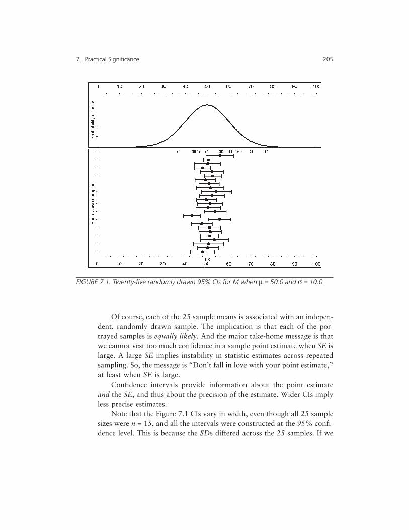
Of course, each of the 25 sample means is associated with an indepen-dent, randomly drawn sample. The implication is that each of the por-trayed samples is equally likely. And the major take-home message is thatwe cannot vest too much confidence in a sample point estimate when SE islarge. A large SE implies instability in statistic estimates across repeatedsampling. So, the message is “Don’t fall in love with your point estimate,”at least when SE is large.

Confidence intervals provide information about the point estimateand the SE, and thus about the precision of the estimate. Wider CIs implyless precise estimates.

Note that the Figure 7.1 CIs vary in width, even though all 25 samplesizes were n = 15, and all the intervals were constructed at the 95% confi-dence level. This is because the SDs differed across the 25 samples. If we


FIGURE 7.1. Twenty-five randomly drawn 95% CIs for M when = 50.0 and = 10.0

had known that σ = 10.0, but somehow still did not know µ, we couldhave drawn CIs to estimate µ, and at fixed n, fixed and known σ, and afixed confidence level, the CIs would have been identical in length. Inpractice, when we are estimating µ, we rarely presume at the same timethat somehow we know σ.

In Figure 7.1, two of the 95% CIs for the M do not capture µ, whichin the present heuristic example is known to be 50.0. These are the 16thand the 17th intervals in Figure 7.1. Of course, in real research, we willnever know that our sample CI does not capture a parameter. Indeed, theestimated precision for the 16th CI is fairly narrow. For this sample result,we might fall in love with our statistic M = ~43, especially given the rela-tively narrow width of the 95% CI. But our love would be misplaced.

If we drew a huge or infinite number of random samples from thepopulation portrayed in Figure 7.1, and constructed 95% CIs for theparameter estimate (e.g., M, SD, coefficient of kurtosis), exactly 95% ofthe intervals would capture the true parameter, and exactly 5% of theintervals would fail to capture the parameter. In other words, when weconstruct a confidence interval, the confidence level statement applies, notto a single interval, but to infinitely many intervals. As Thompson (inpress) emphasized, never forget that 1 ≠ ∞. In the words of Good andHardin (2003), “It is not true that the probability that a parameter isincluded in a [single] 95% confidence interval is 95%” (p. 101).

Thus CIs cannot magically tell us what the parameter we are estimat-ing is. Nevertheless, CIs communicate both the point estimate, and infor-mation about the precision of the estimate. And CIs have the wonderfulfeature that sets of CIs for a literature can readily be presented in a singlepicture. As has been intimated elsewhere (Wilkinson & APA Task Force,1999), a picture may be worth a thousand p values. Such graphics can beeasily constructed with the Excel CHART WIZARD and by inputting CI lowerand upper bounds, as well as the point estimates from a series of studies,as STOCK wizard option low, high, and close values.

Modern software painlessly computes CIs for various statistics, orprovides the relevant SEs. Some very good books that flesh out relatedconcepts have been provided by Altman, Machin, Bryant, and Gardner(2000) and Smithson (2000, 2002). The recent article by Cumming andFinch (2005) provided useful, practical suggestions. As Good and Hardin(2003) explained,


Point estimates are seldom satisfactory in and of themselves. First, if theobservations are continuous, the probability is zero [actually infinitesimallysmall] that a point estimate will be correct and equal the estimated parame-ter. Second, we still require some estimate of the precision of the point esti-mate. (p. 45)

�� Confidence Intervals for Effect Sizes

If effect sizes are essential, and confidence intervals are “the best” report-ing strategy, then the marriage of CIs and effect sizes seems appealing.However, some technical difficulties confront this proposal.

Formulas are available for computing (a) the commonly-used statisticsdiscussed in this book, (b) standard errors for these statistics, and (c) con-fidence intervals for these statistics. But a formula cannot be used to com-pute the CI for an effect size.

The problem with computing a confidence interval for an effect size isthat, unlike CIs for statistics, even for a fixed n the widths of the CIs foran effect size are different for different values of the effect. In essence, adifferent formula for computing an effect CI has to be used for each of theinfinitely many values of the effect size (see Cumming & Finch, 2001).

Nevertheless, CIs for effect sizes may still be computed, but the pro-cess does not involve execution of a formula. Instead, a computer-intensive statistical process called iteration must be used. As convention-ally performed, iteration involves a process of initially guessing a solution,and then repetitively tweaking the guess until some statistical criterion isreached.

Here the logic of iterative estimate of the CI for an effect size is brieflydescribed. For more detail, the reader is referred to Cumming and Finch(2001) and the excellent book by Kline (2004).

In the case of a two-tailed CI, there is a sampling or a test distributionthat is associated with each end of the interval. When we construct aninterval at a given confidence level, 1 – α, for the test statistic distributionfor the left side of the CI, we want α / 2% (e.g., 5% / 2 = 2.5%) of area inthe test statistic distribution to be to the right of the point estimate (e.g.,the computed M, the computed d). Conversely, for the test statistic distri-bution for the right side of the CI, we want α / 2% (e.g., 5% / 2 = 2.5%)


of area in the test statistic distribution to be to the left of the point esti-mate (e.g., the computed M, the computed d).

For CIs for statistics, this outcome can be easily accomplished byinvoking the appropriate computational formula, because only one teststatistic distribution, one assuming the nil null is true, is always used toidentify both endpoints of the confidence interval. But because there areinfinitely many possible test statistic distributions for effect sizes, whichvary in shape for each different effect size, CIs for effect sizes must beiteratively estimated.

The test statistic distributions used in estimating CIs (and also forcomputing power or β) for nonzero effect sizes are noncentral distribu-tions. These are not the central test statistic distributions discussed inChapter 6, which assume a zero effect size, which is the required assump-tion when testing nil null hypotheses. When people say “test statistic,”they are talking about the central test statistics discussed in Chapter 6,unless they explicitly say “noncentral.”

To compute a CI for an effect size, an initial guess is made about theappropriate noncentral test statistic (see Cumming & Finch, 2001, orSmithson, 2001) for the left arm of the CI. Then the computer tweaks theselection of the test statistic distribution, associated with different nonzeroeffect sizes, until α / 2 of the area in the rightmost part of the distribution isjust to the right of the calculated effect. Then the same process is followed in-dependently for the rightmost arm of the effect size CI, or vice versa.

Various computer programs are readily available for iteratively, pain-lessly estimating the CIs for effect sizes. Some run stand-alone (Steiger &Fouladi, 1992), or under SPSS or SAS (Algina & Keselman, 2003; Algina,Keselman, & Penfield, 2005; Smithson, 2001), or Excel (Cumming &Finch, 2001).

Table 7.2 presents a hypothetical literature consisting of 10 studies,and the related Cohen’s d and pCALCULATED values. Nine of the 10 originalstudies and the new 11th study were created to honor Rosnow andRosenthal’s (1989b) view that “surely, God loves the .06 [level of statisti-cal significance] nearly as much as the .05” (p. 1277).

In a literature prejudiced against statistically nonsignificant results,the first study with an anomalous negative effect size (d = –0.50;pCALCULATED = 0.043) will be afforded priority for publication. The remain-ing studies with positive values for d, but p is approximately 0.06, maynever see the light of the publication day.


These dynamics are troubling. If 1,000 researchers all drew randomsamples from a population exactly described by the nil null, and in each ofthe 1,000 independent studies α = 0.05, exactly 50 studies should obtainstatistically significant results. These Type I errors will be afforded publi-cation priority. But subsequently, any researchers replicating the 50 pub-lished studies, each involving Type I errors, will have difficulty publishingtheir failures to replicate statistical significance. In this manner the self-correcting features of science may be compromised by the bias against sta-tistically nonsignificant results. Greenwald (1975, pp. 13–15) cited real-world examples of these dynamics.

Figure 7.2 graphically presents the CIs for the Cohen’s d values fromthe 11 studies. The figure also portrays the weighted (by n) averages foreffects across the studies, and the related CIs. (In real meta-analytic inte-grations of effect sizes, more sophisticated forms of weighted averages areactually used.)

The figure illustrates how a literature can be summarized in a picture.


TABLE 7.2. Integration of d across 11 Hypothetical Studies

Study d n tCALCULATED pCALCULATED

Previous research

1 –0.50 19 –2.18 0.0432 0.25 60 1.94 0.0583 0.50 17 2.06 0.0564 1.00 6 2.45 0.0585 0.75 9 2.25 0.0556 0.30 43 1.97 0.0567 0.85 7 2.25 0.0668 0.20 90 1.90 0.0619 0.57 13 2.06 0.062

10 0.45 19 1.96 0.065

Pooled weighted (by n) average

0.281 283 4.73 <.001

Current study

11 0.28 45 1.88 0.067

Revised weighted average

0.281 328 5.09 <.001

Even a relatively large literature could be summarized economically. Pic-tures such as Figure 7.2 make clear the patterns of effects across relatedstudies. More importantly, such pictures also convey the precisions ofstudies.

Pictures such as Figure 7.2 are too rarely seen today. Such picturesmight lead to disturbing conclusions about the precisions of various litera-tures on which we depend for evidence-based practices (Odom,Brantlinger, Gersten, Horner, & Thompson, 2005).

Some Key Concepts

Effect sizes should not be interpreted using fixed benchmarks orignoring the context of the study. Instead, effects should be inter-preted by invoking personal value judgments informed by “meta-


FIGURE 7.2. Plot of 95% confidence intervals for d values

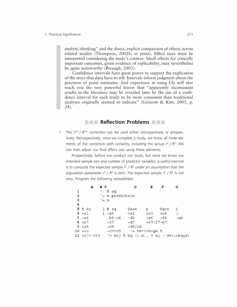
analytic thinking” and the direct, explicit comparison of effects acrossrelated studies (Thompson, 2002b, in press). Effect sizes must beinterpreted considering the study’s context. Small effects for criticallyimportant outcomes, given evidence of replicability, may neverthelessbe quite noteworthy (Breaugh, 2003).

Confidence intervals have great power to support the explicationof the story that data have to tell. Intervals inform judgment about theprecision of point estimates. And experience in using CIs will alsoteach you the very powerful lesson that “apparently inconsistentresults in the literature may be revealed later by the use of a confi-dence interval for each study to be more consistent than traditionalanalyses originally seemed to indicate” (Grissom & Kim, 2005, p.24).


1. The r2* / R2* correction can be used either retrospectively or prospec-

tively. Retrospectively, once we complete a study, we know all three ele-

ments of the correction with certainty, including the actual r2 / R2. We

can then adjust our final effect size using these elements.

Prospectively, before we conduct our study, but once we know our

intended sample size and number of predictor variables, a useful exercise

is to compute the expected sample r2 / R2 under an assumption that the

population parameter r2 / R2 is zero. The expected sample r2 / R2 is not

zero. Program the following spreadsheet.


The output for r2 = 90.0%, n = 10, and one predictor variable will yield

these results.

Under an assumption that the population parameter r2 is zero, solve for

r2* = 0 by varying the input values of r2 and declaring use of only a single

predictor variable for the bivariate problem. The final r2 isolated in this

manner for a given design is the expected sample r2 for the design under

our assumption, and will not be zero, notwithstanding our assumption.

Find the expected sample r2 for (a) n = 15, (b) n = 50, and (c) n = 500,

under an assumption that the population value is zero.

2. Of course, the standardized difference effect sizes are biased by sampling

error, just as other effect sizes are impacted by these same dynamics.

Thus, Hedges (1981; Hedges & Olkin, 1985) proposed a correction factor

for Glass’ ∆. The “adjusted ∆“ can be computed by multiplying the origi-

nal value by the correction factor:

1 – (3/((4 * (nC – 1))–1))

where nC is the sample size in the control group. For example, for nC =

10, the correction factor is the multiplicative constant of 0.91428. Use a

spreadsheet to compute the correction factor for nC = 5, 10, 20, 30, and

40. What does the result suggest about the bias of ∆?

3. Classical effect sizes are “on the average.” Grissom (1994; Grissom &

Kim, 2005) proposed the intriguing alternative idea of a probability of

superiority (PS) effect size that is not on the average, and is computed by


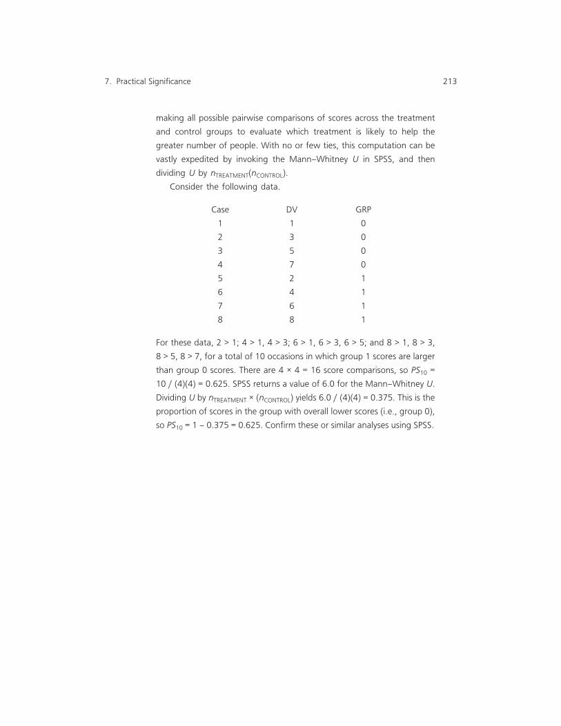
making all possible pairwise comparisons of scores across the treatment

and control groups to evaluate which treatment is likely to help the

greater number of people. With no or few ties, this computation can be

vastly expedited by invoking the Mann–Whitney U in SPSS, and then

dividing U by nTREATMENT(nCONTROL).

Consider the following data.

Case DV GRP

1 1 0

2 3 0

3 5 0

4 7 0

5 2 1

6 4 1

7 6 1

8 8 1

For these data, 2 > 1; 4 > 1, 4 > 3; 6 > 1, 6 > 3, 6 > 5; and 8 > 1, 8 > 3,

8 > 5, 8 > 7, for a total of 10 occasions in which group 1 scores are larger

than group 0 scores. There are 4 × 4 = 16 score comparisons, so PS10 =

10 / (4)(4) = 0.625. SPSS returns a value of 6.0 for the Mann–Whitney U.

Dividing U by nTREATMENT × (nCONTROL) yields 6.0 / (4)(4) = 0.375. This is the

proportion of scores in the group with overall lower scores (i.e., group 0),

so PS10 = 1 – 0.375 = 0.625. Confirm these or similar analyses using SPSS.


8

MultipleRegression Analysis

Basic GLM Concepts

The initial chapters in this book considered situations in which youwish to characterize features of a single variable. Univariate statis-tics characterize features of a single variable as regards (a) location,(b) dispersion, or (c) shape.

Of course, quantitative science focuses on relationships that recurunder stated conditions. So real science at a minimum requires the mea-surement of at least two variables, sometimes conceptualized as a depen-dent (or criterion or outcome) variable, and at least one independent (orpredictor) variable. And in science, the analytic focus is directed specifi-cally at the relationship between these two variables. The bivariate statis-tics that can be used to quantify these relationships include the Pearsonproduct–moment r (or alternatively r2), Spearman’s ρ (or alternativelySpearman’s ρ2), and the φ coefficient (or alternatively φ2).

However, a fundamental premise of statistics is that each researcherpresumes some (conceivably implicit) model of reality. Furthermore, everystatistical analysis tests the fit of a model to data. Consequently, a criticalimperative of social science research is that we ought to insure the fit ofour analytic model with our model of reality. Otherwise we are using our

215

analyses to investigate something other than the reality that we believeexists, which is not sensible!

Our model of reality may posit that the outcome variables of interestto us are multiply caused, or require multiple predictors to attain reason-able predictive accuracy. Given this model of reality, we may well useunivariate statistics, or even bivariate statistics, to understand and describeour variables. But the primary analysis used to address our main researchquestions usually must be able to accommodate multiple predictor vari-ables (and, indeed, sometimes multiple criterion variables).

Multiple regression analysis is a statistical technique that can be usedto investigate relationships between a single outcome variable and two ormore predictor variables. Multiple regression is a univariate statisticalanalysis in the second meaning of the word “univariate” (i.e., analysesinvolving only one outcome variable). Regression is one of many analysesthat can be conducted when only one outcome variable is of interest.

Multiple regression analysis is often of practical value because theanalysis can yield important insights into data dynamics. But regression isjust as important from a heuristic point of view, because regression is theunivariate case of the parametric general linear model (GLM). That is,regression (but not vice versa) can be used to conduct the commonly-usedunivariate statistical analyses.

As Cohen (1968) argued in a seminal article years ago, scholars whounderstand regression understand how the various univariate methods arepart of a single general linear model, what all univariate statistical analy-ses have in common, and what features differentiate the analyses. All sta-tistical analyses (a) are correlational, (b) either explicitly or implicitlycompute weights that are applied to measured (or observed) variables toestimate scores on latent variables (also called synthetic or composite vari-ables), and (c) yield variance-accounted-for effect sizes analogous to r2.

Indeed, there is a broader version of the univariate GLM. Multivariateanalyses (e.g., MANOVA, descriptive discriminant analysis, canonicalcorrelation analysis) simultaneously consider two or more outcome vari-ables and one or more predictor variables. Knapp (1978) and others (e.g.,Thompson, 1991a, 2000a) have explained that canonical correlation anal-ysis is the multivariate general linear model. And there is an even largerGLM umbrella called structural equation modeling (SEM; Bagozzi,Fornell, & Larcker, 1981).


The existence of the multivariate GLM is noteworthy here, becauseonce someone has truly mastered interpretation of results for the regres-sion case, one has all the requisite skills for interpreting multivariateresults. Mastering univariate GLM concepts is like being in Oz with rubyslippers. You can easily branch out to Kansas or multivariate statisticswhenever a good witch (or nice scholar) explains that you now have pow-ers beyond those that may at first glance be obvious.

�� Purposes of Regression

Regression can be used for two purposes: prediction and explanation (i.e.,theory testing). Of course, these purposes are not mutually exclusive.When in real life we do prediction, even when the prediction is very accu-rate, we probably would feel more comfortable if we understood why theprediction worked so well. Conversely, when we test theory, although ourinitial purpose may be basic science (i.e., knowledge for its own sake), wedo usually presume that our insight will ultimately have some practical useof some sort. However, in both cases (and throughout the general linearmodel), the dependent variable is the focus of all analyses.

Focal Role of Dependent Variables

In science, dependent variables are the foci of our thinking, and of all anal-yses. Scientists identify dependent variables that are important to them, orto society. After making the necessary value judgment that given outcomesare important, only then will independent variables be selected. We usetheory, or previous research, or both to inform the selection of those inde-pendent variables that we believe causally control, or predict, or explainthe dependent variables upon which we have decided to direct our atten-tion.

Scholars are systematic in the selection of these independent variables.True, very important insights can be discovered through happenstance.For example, Fleming discovered penicillin when some mold apparentlycame in through an open basement window, landed on some Petri dishes,and killed some of the bacteria growing there. The happenstance was par-

8. Multiple Regression Analysis 217

ticularly fortuitous because this happened just before World War II, whenpenicillin was especially needed in treating very large numbers of wound-related infections. But real science is more than the capitalization on fortu-itous discoveries.

By the same token, in science we do not typically select possible causalvariables and then ask what outcomes these variables might produce. Wedo not usually mix chemicals in various random ways in the hope thatsomething important may eventually occur. Instead, we presume that themost productive progress in generating knowledge occurs when we firstselect outcomes that we value, and then systematically identify promisingpotential predictor variables.

Prediction

Prediction of important outcomes can be valuable, even when we have nounderstanding as to why the prediction works. For example, long ago inEngland smallpox epidemics were killing large proportions of the popu-lace. Jenner discovered that milkmaids died infrequently from smallpox,and subsequently realized that cows get a disease like smallpox in appear-ance, but that is rarely fatal. Jenner reasoned that the milkmaids also gotsmallpox from their cows, which somehow inoculated the milkmaidsagainst subsequent smallpox infection. His informal experiment, in whichhe applied cowpox puss only to selected friends, yielded the confirmationof a causal mechanism, although his social circle was somewhat more con-stricted following his research!

In predictive applications of regression, the existence of two groups ofparticipants is always implied. We have an outcome that we want to pre-dict in our second group of participants (e.g., the grade point averages ofdoctoral students upon their graduation) that has not yet occurred. Per-haps we wish to use these predicted outcome scores of the applicants tomake admission decisions.

We also have our first group of participants. For these participants(e.g., doctoral students who graduated at the university during the previ-ous 3 years), we know the scores on the outcome variable of interest. Wealso have available for this group scores on a range of predictor variables


that might predict graduate grade averages. We conduct the regressionanalysis within group 1.

Iff the prediction works reasonably well in group 1, we then may con-sider using the same predictor variables in group 2. We also will apply theweights generated in group 1 to the predictor variable scores in group 2.The role of these weights is to optimize the accuracy of the prediction.

This use of group 1’s weights with group 2’s predictor variables turnson the fundamentally important assumption that the two groups of stu-dents are reasonably similar. This assumption might not be tenable, forexample, if the two student groups were measured at disparate times, or attwo very different universities, or if the academic majors of the two groupswere very different.

Explanation

Sometimes basic science is conducted simply for the joy of knowing, with-out any expectation of an immediate application of the new knowledge.For example, when we practice science to discover the age of the universe,or its origins, we have little expectation of some immediate use for ournew insights.

Kerlinger (1977) argued that sometimes theories deemed potentiallyuseless at their origination prove in the long term to have greater applica-tion than even the findings from some applied or predictive research, and“science, then, really has no other purpose than theory” (p. 5). For exam-ple, in the 1930s, three scientists working at Bell Laboratories—funded bythe then monopoly of the national telephone system—passed an electricalcurrent through a silicone crystal structure and observed a change in fea-tures of the current. They did not envision the hugely important applica-tions of their discovery in the form of transistors and, later, computerchips. Similarly, in 1905, when Einstein published a series of papers pre-senting his relativity theory, that objects moving faster experience timemore slowly, and his theory that energy and matter are interchangeable,he did not envision that only a few decades later he would type a letter toFranklin Roosevelt to inform the President of the potential use of theoryto guide the creation of an atomic bomb.


�� Simple Linear Prediction

Ultimately, we will consider three multiple regression situations: (a)uncorrelated predictor variables, (b) correlated predictor variables, and (c)correlated predictor variables involving suppression effects. However, firstwe will spend considerable time elaborating simple regression (i.e., regres-sion involving only a single predictor variable). Although not true multipleregression, this simple situation will facilitate laying the groundwork forconsideration of the more complicated (and realistic cases) involving twoor more predictor variables.

It might be noted that the situation involving a single predictor is aspecial case (i.e., a subset) of situation #1, because when only a single pre-dictor is involved, there is no correlation between variables within the pre-dictor variable set. Thus, many of the conclusions about simple linearregression, involving a single predictor, will generalize to the multipleregression situation involving multiple predictor variables that are per-fectly uncorrelated with each other.

Table 8.1 presents the hypothetical data for 20 participants that willbe employed to make this discussion more concrete. The interested readercan readily reproduce or further explore the results presented in this chap-ter for these data by analyzing the data using SPSS or another statisticalpackage.

Form of the Regression Equation

As an example of simple linear regression, one might wish to predict theheight of adults (Yi) using information about their heights at 2 years of age(Xi). Or, alternatively, we might wish to predict the height of adults (Yi)using information about the participants’ IQ scores measured at age 6(Xi).

Regression analysis employs two types of weights: an additive con-stant, a, applied to every individual ith participant, and a multiplicativeconstant, b, applied to the predictor variable for each individual ith partic-ipant. We do not use i subscripts for these constants, because their valuesdo not change across individual participants. Thus, the weighting systemtakes the form of a regression equation:

Yi <—— �Y i = a + b (Xi)


The regression equation is the set of weights generated in a given analysis.Just to keep people on their toes by creating potential confusion, the b

weights are also sometimes synonymously referred to as unstandardizedregression weights. This label is especially confusing, because a constantcannot be standardized. The intent presumably is to refer to “weightsapplied to measured variables in their unstandardized form.”

For example, it is known that the following system of weights worksreasonably well in predicting height at age 21 from height at age 2:

Yi <—— �Y i = 0.0 + 2.0 (Xi)

Thus, an individual such as Kelly, who is XKELLY = 27″ tall at age 2, is pre-dicted to have a height of �YKELLY = 54″ (0.0 + 2.0 × 27 = 0.0 + 54.0 = 54.0)at age 21.


TABLE 8.1. Heuristic Data for Three Regression Situations

Predictor variables

ID/statistic Y X1 X2 X3 X4 X5 X6 X7

1 49.553 48.473 51.610 49.338 49.162 49.718 49.488 50.2402 50.094 48.812 50.537 51.545 50.576 49.640 49.925 51.2863 50.799 49.152 49.732 49.890 50.386 49.662 49.889 50.6414 50.778 49.491 49.195 48.786 49.646 50.297 51.399 51.1165 50.296 49.830 48.927 49.338 50.579 49.924 49.732 49.9046 51.420 50.170 48.927 50.662 50.598 50.704 50.303 50.2237 49.582 50.509 49.195 51.214 48.595 49.350 48.549 49.0958 50.345 50.848 49.732 50.110 49.087 51.979 49.566 48.0049 49.988 51.188 50.537 48.455 50.386 48.923 49.148 51.652

10 50.860 51.527 51.610 50.662 50.806 50.068 49.481 49.78111 49.753 50.170 48.927 50.662 49.768 51.384 49.325 48.40012 50.491 50.509 49.195 51.214 51.681 49.026 50.357 49.84113 48.415 50.848 49.732 50.110 48.873 49.657 50.294 49.37814 49.474 51.188 50.537 48.455 51.746 48.945 51.679 50.99715 49.506 51.527 51.610 50.662 49.755 50.467 50.510 50.22416 47.166 48.473 51.610 49.338 48.393 49.058 47.365 49.21017 50.480 48.812 50.537 51.545 50.857 48.217 50.556 51.48818 51.158 49.152 49.732 49.890 50.760 50.537 50.344 49.27519 49.067 49.491 49.195 48.786 49.834 50.541 51.022 50.03020 50.778 49.830 48.927 49.338 48.512 51.904 51.070 49.216

M 50.000 50.000 50.000 50.000 50.000 50.000 50.000 50.000SD 1.000 1.000 1.000 1.000 1.000 1.000 1.000 1.000

We can also compute a fourth score in regression. If Kelly’s actualheight at age 21 is YKELLY = 60″, we can compute an “error” score as thedeviation between Kelly’s actual height (i.e., YKELLY = 60″) and Kelly’s pre-dicted height (i.e., �YKELLY = 54″). Because ei = Yi – �Y i, for Kelly we haveeKELLY = 6 (i.e., 60 – 54). Any individual whose actual Yi score is perfectlypredicted has ei = 0.0, and iff all participants’ Yi scores are perfectly pre-dicted, all the ei scores will be zero.

The regression problem can also be conceptualized using a scattergramplot. The line of best fit to the data points is the graphical representation ofthe regression equation (i.e., the regression line actually is the regressionequation, and vice versa). The a weight is the point on the vertical Y axis atwhich the regression line crosses the Y axis when X is 0; this is called theintercept. The b weight is the slope (i.e., change in rise/change in run) of theregression line (e.g., the line changes in b units of Y for every change of1 unit of X, 2 times b units of Y for every 2 units of change in X, etc.).

Two Types of Variables

A foundational concept in statistics is the fact that all analyses involve atleast two each of two kinds of variables: measured and latent. In the pres-ent example, both height at age 2 and height at age 21 are measured (orobserved) variables. These are directly measured, without invoking anyweights. But the �Y i and the ei scores are latent (or synthetic or composite)variables.

In actuality, the latent variables are the focus of statistical analysis.These are the variables that represent estimated scores on unobservabletheoretical constructs. And the latent variable �Y i (a) encapsulates all theuseful predictive variability in the predictors and (b) discards all the use-less (nonpredictive) variability in all the predictors. For this reason, the rof Yi with �Y i always equals the r of Yi with Xi (and the r2 of Yi with �Y i

always equals the r2 of Yi with Xi).

Function of the Weights

The function of the weights is to make the Yi and the �Y i scores of a givenith individual match as closely as possible, given the predictive power of agiven Xi. We can think of a range of possibilities, running from perfect


prediction (i.e., every Yi = �Y i for each ith individual, and every ei = 0.0) toprediction involving a useless predictor.

Let’s consider the worst-case scenario first, and then compare thesedynamics to those occurring in a best-case scenario. Of course, in actualresearch we invariably find ourselves somewhere along this continuum ofoutcomes, rather than at one of the two conceptual extremes.

Worst Case

In a worst-case scenario, we have access only to useless predictors. Forexample, let’s assume we are predicting the height of adults (Yi) usinginformation about their IQ scores measured at age 6 (Xi), and the predic-tive information is completely useless.

In a best-case scenario, every Yi = �Y i for each ith individual, and everyei = 0.0. In the best-case scenario, because every Yi = �Y i, every statistic (e.g.,M, Mdn, SOS, SD, coefficient of skewness) computed for Y exactly equalsthe corresponding statistic (e.g., M, Mdn, SOS, SD, coefficient of skew-ness) computed for �Y i, because in fact in this extreme scenario the twovariables have exactly the same data.

But even in a worst-case scenario, we use our weights to optimize thefit of �Y i to Yi. What, if anything, can our weights accomplish in the unfa-vorable situation of a worst-case prediction?

In a worst-case scenario, we will want to obliterate our useless predic-tor variable. Use of a b weight of zero will accomplish this objective quitenicely. When b = 0.0, Xi can have no impact on the estimation of Yi, asquite rightly should be the case. Multiplication by 0.0 kills, and so multi-plication of Xi by b = 0.0 kills the useless predictor.

So now the job of optimizing the fit of �Y i to Yi falls solely to the aweight. Our expectation is not that the weights always do a perfect job ofoptimizing fit. Instead, our expectation is that the weights must optimizethe fit �Y i to Yi within the limits of our data.

We may not be able to do a very good job of optimizing this fit withina worst-case scenario, but what is the best we can do? Remember fromChapter 2 that the mean has the property that the sum of the deviationscores from M is always zero. The implication is that in a worst-case pre-dictive scenario the best (not good, just best) prediction we can accomplishis to set every �Y i to equal MY.


In a worst-case scenario, because b = 0.0, we can set every �Y i equal toMY by setting a = MY. Doing so will optimize the fit of �Y i to Yi, because theei scores will be minimized, just as M minimizes the sum of the deviationscores.

In a worst-case scenario, Yi, Xi, and ei will be variables (two measured,one latent), but the �Y i will be a constant (each equaling MY). There will beonly three variables, not four.

Notice that even in a worst-case scenario the mean of the �Y i scores willequal MY. Of course, at the other extreme of best case, perfect prediction,the mean of the �Y i scores would also equal MY because these two variableswould involve identical data. The implication is that the a and b weightscan make the means of the Yi and the �Y i scores equal throughout every sit-uation, ranging from worst-case to best-case scenario.

Ideally, we would also like the dispersion of the Yi and the �Y i scores tobe equal. However, in the worst-case scenario, the �Y i scores have theirminimum possible dispersion—such that range, SOS, variance, and SD allequal zero—because the �Y i scores in a worst-case scenario are all equal toMY, and define a constant.

Best Case

In the best-case scenario, every Yi = �Y i for each ith individual, and everyei = 0.0. So, in the best-case scenario, Yi, Xi, and �Y i are variables (two mea-sured and one latent), but the ei scores are a constant. In all other situa-tions, regression involves at least two measured variables and exactly twolatent variables.

Of course, in the best-case scenario, as in every possible scenario, themean of the �Y i scores equals MY. But in the best-case scenario, because thedata for the Yi and the �Y i scores are identical, the SOSs of the Yi and the �Y i

scores are also now equal. And because the ns for the two variables areequal, the variances and the SDs of the Yi and the �Y i scores are also equal.

Indeed, the dispersion of the �Y i scores can never exceed the dispersionof the Yi scores. If the SOSY scores equals 22.2, even before conductingany analyses, we know that the dispersion of the �Y i scores cannot be lessthan zero (ever) and that for our data the SOS of the �Y i scores cannotexceed 22.2 (and will only equal 22.2 in a best-case scenario).


Of course, as we learned in the Reflection Problems for Chapters 2and 3, additive weights applied to variables do not affect dispersion. Butmultiplicative weights affect both the dispersion of variables (unless themultiplicative constants are –1 or 1) and the location of variables (unlessthe original mean is zero or the multiplicative constant is 1). Thus, in abest-case scenario, the function of the b weight is to make the dispersionsof the Yi and the �Y i scores equal, while the a and the b weights togethermake the means of the Yi and the �Y i scores equal.

Computation of the Regression Weights

The previously described form of the regression equation presumed thatwe were working in the unstandardized score world. An alternative formof the prediction equation involves first converting both variables intoz-score form (i.e., scores transformed to have a mean of 0.0 and an SD of1.0 via the algorithm zi = (Xi – MX) / SDX) and working instead in the stan-dardized score world.

When all the variables are in z-score form, the a weight is still present,but is always zero. Therefore, the regression equation for standardizedmeasured variables simplifies to the form

ZY <—— �Y = +β(ZX)

Note that the multiplicative weight for this situation is always distin-guished from the multiplicative weight for the nonstandardized scores byreferring to the weights for z scores as β weights (versus b weights).

Just to be confusing, the β weights are also sometimes labeled stan-dardized regression weights. Unfortunately, this label is an oxymoron,because a constant cannot be standardized. What is intended is a referenceto “weights applied to measured variables in their standardized forms.”

Note that the a, b, and β weights are all in the score world, which isnecessary for them to be applicable to the scores also located in this world.However, a and b are in the unstandardized score world, whereas the βweights are in the standardized score world.

It happens that for a two-variable regression problem, the β weight topredict zY with zX is the bivariate correlation coefficient between the two


variables (of course, so is the β weight to predict zX with zY, because rYX =rXY).

The b and β weights can readily be transformed back and forth intoeach other with the equation

b = β(SDY / SDX) (8.1)

or

β = b(SDX / SDY) (8.2)

As the equations imply, b and β will be equal when (a) either is zero or (b)the two variables’ standard deviations are equal. Of course, the equationsalso imply that b and β always have the same signs, because the SDs can-not be negative and so cannot influence the signs of the weights. Andwhen two measured variables are uncorrelated, rXY = b = β = 0.

In essence, as suggested by Equation 8.1, the b weight is computed toremove the standard deviation of X from �Y via division, and attempts toinsert the SDY via multiplication. We do this because we care only aboutthe dependent variable. Any value for a predictor variable is derivativesolely from the predictor’s ability to predict or explain Y.

Table 8.2 presents the bivariate correlation matrix associated with theTable 8.1 heuristic data. Given these results, the equation for predicting zY

with zX would be

zY <—— �Y i = +0.0878(zX)

As noted in Chapter 5, it happens that regression lines (and the relatedplanes or hyperplanes when there are three or four or more measured vari-ables) always pass through the means of all the measured variables.Because the means of both Y and X1 for the Table 8.1 data are 50, theregression line pivots on the Cartesian coordinate where MY = 50.0 andMX1 = 50.0. Furthermore, because for these data both SDY and SDX areequal, as reported in Table 8.1, for these data the b multiplicative weightalso equals β = +0.0878.

And given the form of the prediction equation, �Y i = a + b(Xi)—because


when Xi = MX, then �Y i = MY (merely another way of saying the regressionline pivots on the Cartesian coordinate of the two means)—we can solvefor a as

a = �Y i – b(Xi) (8.3)

or, equivalently, for the mean value of X, as

a = MY – b(MX) (8.4)

Thus, here a equals

45.61 = 50.0 – 0.0878(50.0)

For these two variables in their standard score form, involving meansof zero for both variables, and because here β = b = +0.0878, the a weightfor the standardized variables would be

0 = 0.00 – 0.0878(0.00)

Indeed, for standardized variables, the a weight is always zero, as correctlysuggested by this equation.

These various dynamics are illustrated in the Figure 8.1 plot of the


TABLE 8.2. Bivariate Correlation Matrix

Predictor variables

Variable Y X1 X2 X3 X4 X5 X6 X7

Y 1.0000X1 0.0878 1.0000X2 –0.3795 0.0000 1.0000X3 0.2170 0.0000 0.0000 1.0000X4 0.4819 0.1757 –0.0053 0.1247 1.0000X5 0.2903 0.1426 –0.3929 –0.0795 –0.3758 1.0000X6 0.4392 0.1525 –0.3123 –0.1864 0.4213 0.1671 1.0000X7 0.1740 –0.1400 0.2691 –0.1437 0.5089 –0.6302 0.3542 1.0000

data and the regression line that best fits the data. Note that the regressionline is relatively flat, because the correlation coefficient (and b and β, forthese data) is nearly zero.

Table 8.3 presents related concepts from the perspective of the indi-vidual scores of the 20 participants. Because we select the regression equa-tion to yield the best possible prediction of Y for the group as a whole, onthe average, then it is no surprise that the mean e score is always zero. Thisis part of an operational definition of a “best-fit” position for the regres-sion line.

The sum of squares of the �Y scores (0.147, i.e., the explained disper-sion or variability in Y) plus the sum of squares of the e scores (18.857,


FIGURE 8.1. Y predicted with X1.

229

TAB

LE8

.3.

Ob

serv

edan

dSy

nth

etic

Var

iab

leSc

ore

sPr

edic

tin

gY

wit

hX

1

Mea

sure

dva

riab

les

Lat

ent

vari

able

s

Cas

e/st

atis

tic

YM

Yy

y2X

1� Y

M� Y

� y� y2

ee2

149

.553

50.0

-0.4

490.

201

48.4

7349

.866

50.0

-0.1

340.

018

-0.3

130.

098

250

.094

50.0

0.09

30.

009

48.8

1249

.896

50.0

-0.1

040.

011

0.19

80.

039

350

.799

50.0

0.79

70.

636

49.1

5249

.926

50.0

-0.0

740.

006

0.87

30.

763

450

.778

50.0

0.77

60.

603

49.4

9149

.955

50.0

-0.0

450.

002

0.82

30.

677

550

.296

50.0

0.29

40.

087

49.8

3049

.985

50.0

-0.0

150.

000

0.31

10.

097

651

.420

50.0

1.41

92.

012

50.1

7050

.015

50.0

0.01

50.

000

1.40

51.

974

749

.582

50.0

-0.4

190.

176

50.5

0950

.045

50.0

0.04

50.

002

-0.4

630.

214

850

.345

50.0

0.34

30.

118

50.8

4850

.075

50.0

0.07

40.

006

0.27

00.

073

949

.988

50.0

-0.0

140.

000

51.1

8850

.104

50.0

0.10

40.

011

-0.1

160.

014

1050

.860

50.0

0.85

80.

737

51.5

2750

.134

50.0

0.13

40.

018

0.72

60.

527

1149

.753

50.0

-0.2

480.

062

50.1

7050

.015

50.0

0.01

50.

000

-0.2

620.

069

1250

.491

50.0

0.48

90.

240

50.5

0950

.045

50.0

0.04

50.

002

0.44

60.

199

1348

.415

50.0

-1.5

872.

517

50.8

4850

.075

50.0

0.07

40.

006

-1.6

602.

754

1449

.474

50.0

-0.5

280.

278

51.1

8850

.104

50.0

0.10

40.

011

-0.6

300.

398

1549

.506

50.0

-0.4

950.

246

51.5

2750

.134

50.0

0.13

40.

018

-0.6

280.

395

1647

.166

50.0

-2.8

368.

040

48.4

7349

.866

50.0

-0.1

340.

018

-2.7

007.

290

1750

.480

50.0

0.47

80.

229

48.8

1249

.896

50.0

-0.1

040.

011

0.58

40.

341

1851

.158

50.0

1.15

71.

337

49.1

5249

.926

50.0

-0.0

740.

006

1.23

21.

519

1949

.067

50.0

-0.9

350.

873

49.4

9149

.955

50.0

-0.0

450.

002

-0.8

880.

789

2050

.778

50.0

0.77

60.

603

49.8

3049

.985

50.0

-0.0

150.

000

0.79

30.

629

Tota

l10

00.0

019

.00

1000

.00

1000

.00

0.14

70.

000

18.8

57M

ean

50.0

050

.00

50.0

00.

000

–=

–=

i.e., the unexplained variability in Y) exactly (within rounding error)equals the sum of squares total (SOSY = 19.000). We can even look at thee scores to find the person who most deviates from the regression line (per-son #16). In Figure 8.1, the e scores are the distance, always in verticalunits of Y (because Y is what we care about; the focus of the entire analy-sis is on Y units), of a given �Y i score from the regression line.

The sum of squares explained divided by the sum of squares of Y tellsus the proportion of the variability of individual differences in Y that wecan explain with the predictors. Therefore, for the simple linear regressionsituation,

r2YX = SOSY / SOSY (8.5)

We are dividing an area-world statistic by another area-world statistic,thereby obtaining an area-world result.

In the multiple regression case, we can compute the squared multiplecorrelation coefficient in a corresponding manner, using the equation

R2 = SOSY / SOSY (8.6)

Conversely, given the r2YX (or the R2), we can compute the SOS of the �Y

scores, called the SOSEXPLAINED (or, synonymously, the SOSMODEL,SOSREGRESSION, or SOSBETWEEN), using the formula

SOSEXPLAINED = r2YX(SOSY) (8.7)

for the simple linear regression situation, or

SOSEXPLAINED = R2 (SOSY) (8.8)

for the multiple regression situation.Table 8.4 makes these and some other important points. As expected,

the r of Y with X1 equals the r of Y and �Y, because �Y is all the useful partsof any and all the predictors with all the useless parts of the predictorsdeleted.

It is also noteworthy that predictors and ei scores always have r (and r2)equal to zero. This only makes sense, because the error variability is the


variability in the Y scores that the predictors cannot explain. Finally, thefact that the explained and the unexplained variability in the Y scores areboth conceptually discrete directly suggests the truism that the r (and r2) ofthe �Y i and the ei score also always equals zero.

Required Assumptions

All statistical models provide accurate estimates only when model assump-tions are met. Thus, to the extent that assumptions are imperfectly met,estimates of statistics such as r2, R2, the weights, and pCALCULATED will besomewhat compromised. Of course, we can never perfectly meet theassumptions of statistical methods, but we should at least do so approxi-mately, and when interpreting our results, we must bear in mind thedegree to which assumptions are met. If we deem that assumptions are notmet to an acceptable degree, alternative analyses that make fewer orweaker assumptions must be considered.

Here are the primary statistical assumptions of regression:

1. Scale. The dependent variable is at least interval, and the indepen-dent variables are either dichotomous or at least intervally-scaled.

2. Model specification. We are using (a) the correct predictor vari-ables, and (b) only the correct predictor variables, and (c) the formof relationships (e.g., only linear relationships are considered,curvilinear relationships are modeled) being modeled is correct.


TABLE 8.4. Correlation Coefficientsamong Two Observed and Two Synthetic Variables

SPSS Variable Names

Variable Y �Y e X1

Y 1.0000 0.0878 0.9961 0.0878�Y 0.0878 1.0000 0.0000 1.0000e 0.9961 0.0000 1.0000 0.0000X1 0.0878 1.0000 0.0000 1.0000

Note. rY × X = r of Y with �Y. rS, the structure coefficient, = r of X1 with �Y. r of e with �Y always= 0. r of e with X1 always = 0.

3. Error scores. The ei scores are normally distributed in the popula-tion.

4. Homoscedasticity. In the population the ei scores have equal vari-ances at different values of the predictor variables.

5. Predictors imperfectly correlated. No predictor is a perfect linearcombination of (i.e., is perfectly correlated with) any linear combi-nation of the other predictor variables.

�� Case #1: Perfectly Uncorrelated Predictors

Regression analysis is also relatively straightforward in the situation ofmultiple predictors that are perfectly uncorrelated. This sounds like animprobable occurrence, but in practice it occurs quite frequently, as whenwe employ as predictors certain kinds of scores from factor analysis(Thompson, 2004) or when we perform certain analyses called balancedANOVA models, as we will see in subsequent chapters.

As noted previously, the use of a single predictor is a special case ofhaving multiple predictor variables that are uncorrelated with each other,and many of the same dynamics occur for both situations. For example,when there is a single predictor, or when multiple predictor variables areperfectly uncorrelated with each other, the r of each predictor with the de-pendent variable is that predictor’s individual β weight. This is illustratedin the Table 8.5 results involving the prediction of Yi with perfectlyuncorrelated predictors X1i, X2i, and X3i.

Table 8.5 also presents the structure coefficient (rS) for each predictorvariable. A regression structure coefficient (Cooley & Lohnes, 1971, p. 55;Thompson & Borrello, 1985; Thorndike, 1978) is the bivariate correlationof a measured predictor with the latent �Y scores (not with the Y scores), andis very useful in giving us a better understanding of the structure or thenature of the synthetic variable. Understanding the structure or makeup ofthe latent variable scores can be very important in understanding the predic-tive utility of the predictor variables, as various researchers have emphasized(cf. Courville & Thompson, 2001; Dunlap & Landis, 1998). As Thompsonand Borrello (1985) explained, a predictor can have a β weight of zero, but


can actually be an exceptionally powerful predictor variable. One mustlook at both β and structure coefficients when evaluating the importance ofa predictor, as we shall see in some detail in Chapter 9.

Table 8.6 makes clear that something else intriguing happens whenthe predictors are perfectly uncorrelated: the sum of the r2s for the predic-tors (each representing proportionately how much of the dependent vari-able’s variability a predictor can explain) will equal the R2 involving all thepredictors because, in this situation, the predictors do not overlap at allwith each other. Thus, 0.0077 + 0.1440 + 0.0471 = the R2 of 19.88%.

We can see these dynamics mathematically within one of the manyformulas for computing the squared multiple correlation, which appliesacross all regression cases, for any number of predictors 1 through j:

R2 = β1(rY × X1) + β2(rY × X2) + . . . + βj(rY × Xj) (8.9)

However, iff we are in Case #1, because each β weight equals the correla-tion of a given predictor with Y, we can reexpress the equation as


TABLE 8.5. Regression Results for Predicting Y with X1, X2, and X3;X4, X5, and X6; or X4, X5, and X7

Statistics

Case predictors β r Partial r rS

Case #1X1 0.0878 0.0878 0.0977 0.1970X2 –0.3794 –0.3795 –0.3903 –0.8511X3 0.2170 0.2170 0.2356 0.4866

Case #2X4 0.6418 0.4819 0.5791 0.6844X5 0.5177 0.2903 0.5287 0.4123X6 0.0824 0.4392 0.0865 0.6238

Case #3X4 0.5841 0.4819 0.5971 0.6517X5 0.7169 0.2903 0.6359 0.3926X7 0.3285 0.1740 0.3310 0.2354

Note. In Case #1, a given β = rY with X. In all cases, rS = rY with X / R.

R2 = rY × X1(rY × X1) + rY × X2(rY × X2) + . . . + rY × Xj(rY × Xj) (8.10)

or as

R2 = rY × X12 + rY × X2

2 + . . . + rY × Xj2 (8.11)

�� Case #2: Correlated Predictors,No Suppressor Effects

Collinearity (or multicollinearity) refers to the extent to which the predic-tor variables have nonzero correlations with each other. Computationsbecome appreciably more complicated when the predictors are collinear.The β weights for given predictors no longer equal the rs for the same pre-dictors with the Yi scores, as reflected in Table 8.5. And as reported inTable 8.6, the rs no longer sum to R2 (i.e., the sum, 0.5094, does not equalthe R2 of 49.575%). And notice how in Table 8.5 variable X6 has a near-zero β weight (+0.082372) but an rS of +0.6238.

The challenge when we have correlated predictors is that we must not


TABLE 8.6. Results Associated withTable 8.1 Data and the Prediction

of Y with Variable Sets of Size k = 3

Predictor/sum rY with X r2Y with X

X1 0.0878 0.0077X2 –0.3795 0.1440X3 0.2170 0.0471Sum 0.1988

X4 0.4819 0.2322X5 0.2903 0.0843X6 0.4392 0.1929Sum 0.5094

X4 0.4819 0.2322X5 0.2903 0.0843X7 0.1740 0.0303Sum 0.3468

allow commonly explained variability in Yi to be multiply credited to twoor more predictor variables. We can allocate predictive credit for com-monly explained portions of the Y variability however we wish (e.g., all toX1, all to X2, or split in various ways between the predictors), but thecredit may be given only one time. Otherwise, we might obtain a squaredmultiple correlation greater than 100%, which illogically would assertthat we can explain more variability in the Yi scores than the Yi scoreshave.

For example, conceptually, if two predictors both had r2 with Y of100%, and both predictors were given full credit for their predictive abil-ity, we would obtain an erroneous estimate that R2 = 200%! Logically, werequire a computational formula for the β weights that (a) takes into con-sideration all the r2 values among all the pairs of the measured variables,and (b) allocates predictive credit to predictors such that explained por-tions of the variability in the Yi scores are explained only once.

The number of rs that must be used to compute a single β weight cangrow quite large as predictors are added. For one predictor (i.e., two mea-sured variables, one dependent, one predictor), there is only one r. For twopredictors (three measured variables), according to Equation 6.2,

CPW = [N (N – 1)] / 2 (6.2)

there are [3(3 – 1)] / 2 = three correlation coefficients that must be com-puted. For three predictors (four measured variables), there are [4(4 – 1)] /2 = six correlation coefficients that must be considered. For four predic-tors, there are 10 correlation coefficients that must be considered, and forfive predictors there are 15 coefficients to consider.

To simplify the discussion of how beta weights are computed, we willlimit the discussion to an example involving two predictors. For two pre-dictor variables, the two β weights for all cases can be computed using theequations

β1 = [rY × X1 – {(rY × X2)(rX1 × X2)}] / [1 – rX1 × X22] (8.12)

and

β2 = [rY × X2 – {(rY × X1)(rX1 × X2)}] / [1 – rX1 × X22] (8.13)


Let’s say that rY × X1 = 0.707 and rY × X2 = 0.577. To be in Case #2, rX1 × X2

≠ 0, and we will specify rX1 × X2 = 0.800. So, based on Equation 8.12, wehave

[0.707 – {(0.577)(0.800)}] / [1 – 0.8002][0.707 – {(0.577)(0.800)}] / [1 – 0.640]

[0.707 – {(0.577)(0.800)}] / 0.360[0.707 – 0.462] / 0.360

0.245 / 0.360β1 = 0.682

and

[0.577 – {(0.707)(0.800)}] / [1 – 0.8002][0.577 – {(0.707)(0.800)}] / [1 – 0.640]

[0.577 – {(0.707)(0.800)}] / 0.360[0.577 – 0.566] / 0.360

0.011 / 0.360β2 = 0.032

And, based on Equation 8.9, the squared multiple correlation can becomputed as:

0.682(0.707) + 0.032(0.577)0.482 + 0.018

R2 = 0.500

The score-world multiple R would equal 0.5000.5, or 0.707. One implica-tion of these calculations is that R2, R, and the beta weights can be com-puted given only the bivariate correlation matrix. Thus, reporting thecorrelation matrix for related regression analyses is good practice. Thisallows confirmation by readers of reported results, or the fitting of alter-native regression models.

Note that iff we have perfectly uncorrelated predictors, Equation 8.12

β1 = [rY × X1 – {(rY × X2)(rX1 × X2)}] / [1 – rX1 × X22] (8.12)


can be reexpressed as

β1 = [rY × X1 – {(rY × X2)(0.0)}] / [1 – 0.02] (8.14)

which simplifies to β1 = rY × X1, as noted previously. In parallel fashion, forCase #1, β2 = rY × X2.

�� Case #3: Correlated Predictors,Suppressor Effects Present

However, appreciably more complicated dynamics occur when suppressoreffects are present in the data. As defined by Pedhazur (1982), a possible“suppressor variable is a [predictor] variable that has a zero, or close tozero, correlation with the criterion but is correlated with one or more thanone of the predictor variables” (p. 104). Suppressors improve predictionindirectly by making other predictors better, which cannot happen if thepredictor variables are all perfectly uncorrelated.

To many students, “suppression” sounds like a bad thing. Perhapssuppression sounds like “repression,” which is a Freudian construct notpositively viewed by most psychoanalysts as healthy over the long term.But statistical suppression and psychological repression have nothing todo with each other. Suppressor variables in multiple regression (and inother analyses throughout the general linear model) make the R2 effect sizelarger, even though the suppressor has little or no correlation with the cri-terion variable.

So, suppressor effects are good, though they do complicate the inter-pretation of results. Nevertheless, they honor the kinds of complex rela-tionships that can occur in reality.

Variable X7 in variable set X4, X5, and X7, as predictors of Yinvolves a suppression dynamic, as reflected in the Table 8.2 correlationcoefficients. Notice in Table 8.6 that the sum of the r2 values is 0.3468,but the R2 value for these data is 54.677%, which is larger than the sum ofthe r2 values!

Suppressor effects are quite difficult to explain in an intuitive manner.Horst (1966) presented an actual example that is relatively accessible. He


noted that during World War II the prediction of airplane pilot ability wasa major problem. At the start of the war, many trainees were crashingtheir planes, killing their instructors, or simply failing their final checkoutflights such that precious training was wasted. But lots of data were avail-able on the trainees. Basically, scads of men in World War II upon initialadmission to the armed forces were herded into auditoria, and completedhuge batteries of tests wearing their army-issued boxer shorts.

So psychologists approached this regression prediction problem byusing mechanical, spatial, and verbal abilities—all three predictors beingmeasured with paper-and-pencil tests—to predict the actual checkoutflight ratings of previous trainees (i.e., group 1). If the equation workedwell, new potential flight trainees (i.e., group 2) could be screened into (ornot into) training based on their �Y i scores.

The verbal scores had very low correlations with the dependent vari-able, piloting ability, because flying has no systematic relationship withverbal ability. But verbal scores had larger correlations with the other twopredictors, because the predictor variables were all measured with paper-and-pencil tests (i.e., measurement artifacts confounded the mechanicaland spatial ability scores). As Horst (1966) noted, “Some verbal abilitywas necessary in order to understand the instructions and the items usedto measure the other three abilities” (p. 355).

Counterintuitively, including verbal ability scores in the regressionequation actually served to remove the contaminating influence of the ver-bal predictor from the other predictors, which effectively increased the R2

value from what the effect size would have been if only mechanical andspatial abilities were used as predictors. The verbal ability variable hadnegative b and β weights. As Horst (1966) noted

To include the verbal score with a negative weight served to suppress or sub-tract irrelevant ability, and to discount the scores of those who did well onthe test simply because of their verbal ability rather than because of abilitiesrequired for success in pilot training. (p. 355)

In regression, and throughout the general linear model, measured pre-dictor variables can help predict or explain outcomes (1) directly or (2)indirectly (by improving the predictive power of other predictor variables),or both. The job of the multiplicative weights in regression (and in other


GLM analyses) is to optimize the prediction in any (and every) way theycan.

Let’s look at an extreme example involving two measured predictorvariables, where rY × X1 = 0.707, rY × X2 = 0.000, and rX1 × X2 = –0.707. So,based on Equation 8.12, we have

[0.707 – {(0.000)(–0.707)}] / [1 – –0.7072][0.707 – {(0.000)(–0.707)}] / [1 – 0.500]

[0.707 – {(0.000)(–0.707)}] / 0.500[0.707 – 0.000] / 0.500

0.707 / 0.500β1 = 1.414

and

[0.000 – {(0.707)(–0.707)}] / [1 – –0.7072][0.000 – {(0.707)(–0.707)}] / [1 – 0.500]

[0.000 – {(0.707)(–0.707)}] / 0.500[0.000 – –0.500] / 0.500

0.500 / 0.500β2 = 1.000

And, based on Equation 8.9, the squared multiple correlation can becomputed as

1.414(0.707) + 1.000(0.000)0.999 + 0.000

R2 = 0.999

In this example, the presence of the X2 suppressor variables allows β1 toescape its upper mathematical limit of +1.0 because the β weights are nolonger bivariate correlation coefficients.

The β weights are only Pearson correlation coefficients in Case #1. InCases #2 and #3, the β weights are not correlation coefficients. So, in cases#2 and #3, the words “correlation” and “correlated” should never be usedwhen discussing β weights. Instead, in Cases #2 and #3 the β weights mustbe interpreted as reflecting a number of fractional units (e.g., –1.571) of


change in the �Y scores predicted for a corresponding 1 SD of change in agiven predictor variable, with scores on the other predictors all held con-stant. Unfortunately, in published research this admonition for correctpractice is honored hugely more in the breach than in compliance(Courville & Thompson, 2001).

This last example also makes another very important point: The latentor synthetic variables analyzed in all parametric methods are always morethan the sum of their constituent parts. If we only look at observed vari-ables, by only examining a series of bivariate rs, we can easily under- oroverestimate the actual effects that are embedded within our data. Wemust use analytic methods that honor the complexities of the reality thatwe purportedly wish to study—a reality in which measured variables caninteract in all sorts of complex and counterintuitive ways.

�� Weights versus Structure Coefficients

Debate over the relative merit of emphasizing β weights rather than struc-ture coefficients during result interpretation has been fairly heated (H. R.Harris, 1989, 1992). The position taken here is that the thoughtfulresearcher should always interpret either (a) both the beta weights and thestructure coefficients or (b) both the β weights and the bivariate correla-tions of the predictors with Y.

As noted previously, a regression structure coefficient (Cooley &Lohnes, 1971, p. 55; Thompson & Borrello, 1985) is the bivariate Pearsonr of a measured predictor with the latent �Y scores (not with the Y scores,unless R2 = 1.0). There are two ways to obtain the structure coefficient fora given predictor variable. First, the �Y scores can be computed and thencorrelated with the predictor variables. In SPSS, the �Y scores can beobtained either by using the SAVE=PRED subcommand within theREGRESSION procedure, or by invoking a series of COMPUTE commands.Then the CORRELATIONS procedure is used to obtain the Pearsonproduct–moment correlations of all the predictors with the �Y scores.

Alternatively, for a given predictor variable, the structure coefficient(rS) can be computed using the formula


rS = rX with Y / R (8.15)

This computation is easily accomplished on a hand-held calculator or inExcel. The equation makes clear that structure coefficients are score-worldresults, because both values to the right side of the equal sign are score-world, and no squaring operations have been invoked in the equation.

It has been noted by Pedhazur (1982) that structure coefficients “aresimply zero-order correlations of independent variables with the depen-dent variable divided by a constant, namely, the multiple correlation coef-ficient. Hence, the zero-order correlations provide the same information”(p. 691). Thus, the structure rs and the predictor-dependent variable rswill lead to identical interpretations, because they are merely expressed ina different metric. Because rS = rX with �Y = [rX with Y / R], structure rs andpredictor-dependent variable rs will always have the same sign, because Rcannot be negative, and will equal each other only when R = 1.0.

Although the interpretation of predictor-dependent variable correla-tions will lead to the same conclusions as interpretations of rSs, someresearchers have a stylistic preference for structure coefficients. AsThompson and Borrello (1985) argued,

it must be noted that interpretation of only the bivariate correlations seemscounterintuitive. It appears inconsistent to first declare interest in an omnibussystem of variables and then to consult values that consider the variablestaken only two at a time. (p. 208)

The squared predictor-dependent variable correlation coefficientsinform the researcher about the proportion of Y variance explained by thepredictors. Squared structure coefficients inform the researcher about theproportion of �Y (i.e., only the explained portion of Y) variance explainedby the predictors.

Some researchers object to interpreting structure coefficients, becauserSs are not affected by the collinearity (i.e., the correlations) among predic-tor variables. Beta weights, on the other hand, are affected by correlationsamong the predictors, and therefore may change if these correlationschange, or if any variables in a study are added or deleted. That is, βweights are context-specific to a particular set of measured predictor vari-ables.


However, the insensitivity of rS is not an intrinsic weakness. Becausescience is about the business of generalizing relationships across partici-pants, across variables and measures of variables, and across time, in somerespects it is desirable that structure coefficients are not impacted bycollinearity. This insensitivity honors a reality in which measured predic-tor variables are correlated, and rS is unaffected by this collinearity, whichis instead duly considered when computing the β weights.

On the other hand, when the measured variables in a study are theonly variables of interest for the researcher’s purposes in a fixed context,then one is less concerned by the impacts of collinearity among a fixed setof predictors. Here the context specificity of the β weights is less troubling.Obviously, the utility of statistics, including structure coefficients, variessomewhat from problem to problem or situation to situation.

Other researchers are troubled by the fact that structure rs are inher-ently bivariate. One response is that all conventional parametric methodsare correlational (e.g., Knapp, 1978), and that even a multivariate methodsuch as canonical correlation analysis can be conceptualized as a bivariatestatistic (Thompson, 1991a). Indeed, R itself is a bivariate statistic, albeitone involving a synthetic variable, because

RY with X1, X2, . . . , Xj = rY with Y (8.16)

and

RY with X1, X2, . . . , Xj2 = rY with Y

2 (8.17)

It should also be noted that rS is not really completely bivariate, in that rS isa correlation involving �Y (not the measured variable, Y), and �Y is itself asynthetic or latent variable involving all the predictor variables.

Interpreting only β weights is not sufficient (Courville & Thompson,2001), except in Case #1, or in the one-variable situation, because thenr = β, and rS = 1.0 (unless R = 0.0, in which case rS is undefined). Together,through their stereoscopic representations of data dynamics, the β weightsand the structure coefficients tell the researcher which situation applies tothe data. Three possibilities exist. In these situations, a predictor variablewith both β = 0 and rS = 0 is always clearly and definitely useless, but oth-


erwise the predictor is not definitively useless, and should not be inter-preted as being useless.

Possibility 1

When the β weights of multiple predictors each equal the predictors’respective rs with Y (and each rS = rY with X / R = β / R), then the researcherknows that the predictors are uncorrelated. In this situation, interpretingβ, or structure coefficients, or predictor-dependent variable correlationswill all lead to identical conclusions about the importance of predictorvariables.

Possibility 2

When predictors have nonzero βs, some of which do not equal the predic-tors’ respective rs with Y, then predictor variables are correlated with eachother (i.e., are collinear or multicollinear). Assuming no suppression, theR2 will be less than the sum of the r2s. Both β weights and structure coeffi-cients must be interpreted. And a predictor with a zero or near-zero βweight may have the largest |rS|, and be the best single predictor, albeitbeing denied credit in the context-specific dynamics of the β weights.

Possibility 3

Iff a predictor has, at the extreme, a zero structure coefficient (and a zerocorrelation with Y), the predictor may be a suppressor variable. There aretwo ways to distinguish whether the predictor is merely useless, or insteadis a suppressor variable. First, if this predictor has a nonzero β weight,then suppressor effects are present. Second, if the R2 with the possible sup-pressor included in the analysis is greater than the R2 with the possiblesuppressor not included in the analysis, then this predictor variable is asuppressor. Either of the two strategies will always lead to the same con-clusion about suppression for a given data set.

The importance of understanding suppressor effects is not to suggestthat such predictors should necessarily be sought out when the measuredvariables are selected. Anticipating what predictors may be suppressors in


forthcoming research can be difficult. However, suppression effects arenot uncommon throughout the general linear model, and correct resultinterpretation may turn upon an awareness that these effects can occureven when the dynamics were not anticipated (Tzelgov & Henik, 1991).

�� A Final Comment on Collinearity

As noted previously, collinearity (or multicollinearity) simply refers to thefact that the measured predictor variables have nonzero bivariate correla-tion coefficients with each other. Traditionally, researchers sought predic-tor variable sets in which the predictors had as little bivariate correlationwith each other as possible. This was accomplished in various ways, suchas dropping some predictors that were highly correlated with other predic-tors, or combining highly correlated subsets of predictors into singlescores by averaging or summing the predictors in a given subset, or byother methods. This objective was pursued for several reasons, some ofwhich are no longer relevant.

First, as suggested by Equations 8.12 and 8.13, when predictors arevery highly correlated, precision in the calculation of the β weights maybecome problematic. For example, the denominator in the calculation(e.g., [1 – rX1 × X2

2]) may become quite small. However, this consideration istrivial in the presence of modern computers and software, which accu-rately perform calculations to many more decimal places than was possi-ble when computations were performed by humans using calculators.

Second, investigators sought research situations in which result inter-pretation was simple and straightforward. This is accomplished whenworking in Case #1, because, here, interpreting βs, or structure coeffi-cients, or predictor-dependent variable correlations will all three lead tothe same conclusions about the importance of the predictor variables.However, most researchers posit living in a reality in which measured vari-ables are rarely, if ever, perfectly uncorrelated. Accomplishing simplifiedinterpretation at the expense of creating sets of variables that do nothonor reality may seem too high a price to pay for easier result interpreta-tion.

Third, as predictor variables are more correlated, the standard errors


of the b weights are inflated. Either large correlations among a few predic-tors, or small correlations among a large set of predictors, can be poten-tially problematic. The resulting tCALCULATED (or Wald, or critical ratio) teststatistics for evaluating the nil null hypothesis that a given weight is zerobecomes smaller. And for a given b weight, the same t value applies to therelated β weight. The implication is that with highly correlated predictors,the possibility arises that fewer (and perhaps none) of the weights will bedeemed statistically significantly different from zero.

This problem is less troubling if the weights are instead evaluated bydirect comparison with the values in related prior studies. Interpreting theweights via direct comparison with related results in prior studies alsoavoids the problem that NHSST results in different studies are not compa-rable when studies involve different sample sizes (Ziliak & McCloskey,2004). However, the problem of inflated standard errors is a factor thatwarrants some consideration when researchers are selecting predictor vari-ables, and again when researchers are interpreting results involving corre-lated predictors.

The take-home message is that the explicit, direct comparison ofresults with those in related studies is always very useful (if not vital). Noone study means very much in isolation, at least as regards the particularvalues of the statistical estimates themselves.

Some Key Concepts

Iff the predictors are all completely useless, the b and the β weightswill all be zero, and a will equal MY. Also, given that universally

R2 = β1(rY × X1) + β2(rY × X2) + . . . +βj(rY × Xj) (8.9)

for this situation, R2 will equal zero. Iff R2 = 0, because the b and theβ weights are all zero, the �Y i scores will all equal a and MY, and notconstitute a variable. Iff R2 = 1, the ei scores will all equal zero andnot constitute a variable.

The Yi and the �Y i scores always have the same mean. The mini-mum SD and SOS of the �Y i scores is zero, which occurs iff R2 = 0. Themaximum SD of the �Y i scores is SDY, and the maximum SOS of the �Y i

scores is SOSY. The maximum dispersion of the �Y i scores is reached iffR2 = 1. The β weights are correlation coefficients iff we are in Case#1.


The R2 is an “on the average” characterization of how closely theYi and the �Y i scores match for different participants. Thus, if R2 is50%, this does not mean that the ei scores are equal for each person,and instead some ei may be zero while others are relatively large. Onlywhen R2 = 1 can we apply the characterization of this effect size bothto the dataset generically and across all individuals.


1. Given the use of z scores for all measured variables, when are �Y i scores

also z scores? Given the use of z scores for all measured variables, when

are ei scores also z scores?

2. A researcher tells you only one result from her study: a β = –2.5. List

everything that can be deduced about the design and the study’s results.

3. β weights are correlation coefficients iff we are in Case #1. However, in

all cases, β weights indicate how many units of change will occur in �Y i for

one unit of change in a given predictor variable, holding all other predic-

tors constant. In Chapter 5 it was asserted that r is not itself intervally

scaled. However, in Case #1, if β1 = +1.0 and β2 = +0.5, 1 SD of change in

X1 does yield twice as much predicted change in �Y i than does one unit of

change in X2. Does this mean that in the metric of scores, and not in the

metric of the SOS, r is an intervally-scaled indicator of the relative leverage

of predictors in Case #1?


9

A GLMInterpretation Rubric

Result interpretation strategies must be governed by the researcher’spurpose. The research purpose impacts what coefficients are rele-vant, or what benchmarks are used to evaluate sample results, orboth. For example, in an explanation or theory-testing study, per-

haps the only judgment will be whether the detected effect size (e.g., R2) iscomparable to a theoretically-predicted value, regardless of which predic-tor variables may contribute to the effect. Conversely, in another theory-focused study, perhaps the overall effect size is well established acrossstudies, and will not be of primary interest.

Model specification error occurs when (a) predictor variables thatshould not be used are included in the model, or (b) necessary predictorvariables are omitted, or (c) the incorrect analysis is used (e.g., a linearform of relationships is modeled when relationships are curvilinear orlogistic). If the researcher believes that model specification error is not atissue, then the β weights may be of more interest in interpretation, becausethe context specificity of the weights is not a limitation if the analytic con-text is deemed correctly-specified.

247

But as Pedhazur (1982) has noted, “The rub, however, is that the truemodel is seldom, if ever, known” (p. 229). And as Duncan (1975) hasnoted, “Indeed it would require no elaborate sophistry to show that wewill never have the ‘right’ model in any absolute sense” (p. 101).

Here a generic interpretation rubric, one with wide utility, is offered.Because multiple regression is the univariate general linear model (Cohen,1968), and is a subcomponent within the multivariate general linearmodel (Knapp, 1978), this interpretation rubric has wide applicabilityacross various analyses.

The proposed rubric involves two hierarchical steps. First, theresearcher asks, “Do I have anything?” Second, if and only if (iff) theanswer to the first question is yes, only then does the researcher ask,“Where does my something come from?” It is not logical to obtain noth-ing, and then ask, “From where does my nothing originate?”

�� Do I Have Anything?

Researchers can interpret any combination of three pieces of evidence toaddress the question, “Do I have anything?” Different researchers willmake different choices about what evidence to consider, or differentiallyemphasize different evidence.

Statistical Significance

Some researchers begin interpretation by evaluating the nil null hypothesisthat H0: R2 = 0 (or, equivalently, H0: R = 0). Table 9.1 presents the requi-site calculations. The first step involves computing the SOS of the Yi

scores, using Equation 3.1, or an algebraically equivalent formula. Thissum of squares is sometimes called the SOSTOTAL. This is the variability(i.e., the information about the amount and origins of individual differ-ences) that we are trying to explain using the predictor variables.

Next, the SOSEXPLAINED (SOSMODEL, SOSREGRESSION, SOSBETWEEN) is com-puted. As noted in Chapter 8, once the regression weights are derived, the�Y scores can be computed. Applying Equation 3.1 (or an algebraicallyequivalent formula) to the �Y i scores yields the SOSEXPLAINED.


Then, the SOSUNEXPLAINED (SOSERROR, SOSRESIDUAL, SOSWITHIN) can becomputed. Because the �Y i scores and the ei scores are always perfectlyuncorrelated, SOSEXPLAINED + SOSUNEXPLAINED = SOSTOTAL (SOSY), and theSOSUNEXPLAINED can be computed by subtraction (SOSTOTAL – SOSEXPLAINED).Alternatively, Equation 3.1 can be applied to the ei scores to obtain theSOSUNEXPLAINED.

The regression effect size (R2) can be computed using Equation 8.6(R2 = SOSY / SOSY). If a “corrected” effect size is desired, the regressionanalog of the Ezekiel (1930) correction can be applied to obtain the“adjusted R2”:

1 – ((n – 1) / (n – v – 1))(1 – R2) (9.1)

where n is the sample size and v is the number of predictor variables. Theformula can be equivalently expressed as

R2 – ((1 – R2)(v / (n – v – 1))) (9.2)

Next, the degrees of freedom (df) must be computed. The dfTOTAL

equals n – 1. For multiple regression analysis, the dfEXPLAINED (dfMODEL,

9. A GLM Interpretation Rubric 249

TABLE 9.1. Variance Partitions Summary Table

Source SOS df MS FCALCULATED Effect size

Between groups d f h j kWithin groups e g iTotal a b c

Note. a = d + e.b = n – 1.f = the number of predictor variables in the regression analysis.g = n – 1 – the number of predictors in the regression analysis.b = f + g.h = d / f.i = e / g.c = a / c = SDY

2.c ≠ h + i.j = h / i, assuming i ≠ 0.k = d / a = (a – e) / a.

dfREGRESSION, dfBETWEEN) equals the number of predictor variables. ThedfUNEXPLAINED (dfERROR, dfRESIDUAL, dfWITHIN) can be computed by substraction(dfTOTAL – dfEXPLAINED). Alternatively, the dfUNEXPLAINED can be computed asn – 1 – v, where v is the number of predictor variables.

At this point, we can compute the variance of the Yi scores by dividingthe SOSY by dfTOTAL. However, because the test statistic used for thisNHSST application is the F ratio, an area-world statistic, we also needtwo additional variances to compute FCALCULATED.

We compute the mean square explained (MSEXPLAINED, or MSMODEL,MSREGRESSION, MSBETWEEN) by dividing SOSEXPLAINED by dfEXPLAINED. Note thatthis is also a variance estimate, even though the label used is “meansquare.” We compute the MSUNEXPLAINED (MSERROR, MSRESIDUAL, MSWITHIN) bydividing SOSUNEXPLAINED by dfUNEXPLAINED. Again, the mean square unex-plained is a type of variance, and is an area-world statistic.

Then, when possible, we compute the FCALCULATED by dividing theMSEXPLAINED by the MSUNEXPLAINED. However, if the R2 is 100% (and theSOSEXPLAINED = SOSTOTAL, and SOSUNEXPLAINED = 0), the MSUNEXPLAINED equalszero, and the FCALCULATED is undefined (i.e., cannot be computed). Thismeans that, ironically, we cannot perform NHSST whenever we can per-fectly predict or explain an outcome variable.

Given α, we perform the statistical significance test by comparing theFCALCULATED with dfEXPLAINED and dfUNEXPLAINED with the FCRITICAL withdfEXPLAINED and dfUNEXPLAINED. As noted in Chapter 3, we can obtain theFCRITICAL for any α and any degrees of freedom by invoking the Excel FDIST

statistical function. Alternatively, we can determine the pCALCULATED valueby invoking the Excel FINV statistical function, and then comparepCALCULATED with pCRITICAL to determine whether or not to reject H0: R2 = 0.

Of course, SPSS and other statistical packages automate all these cal-culations. If we wish, we may augment these results by performing “what-if” analyses using the Figure 6.3 spreadsheet. Or we can use the “what-if”spreadsheet proposed by Thompson and Kieffer (2000) instead invoking“corrected R2.”

Effect Size

The regression effect size is R2, or the “corrected” or “adjusted” R2. Theeffect size is an index of the practical significance of results (Kirk, 1996).


As strongly emphasized in Chapter 7, the correct interpretation of effectsizes does not invoke Cohen’s benchmarks for “small,” “medium,” and“large” effects, except perhaps when research is being conducted in aground-breaking venue. Instead, the correct interpretation of resultsfocuses on direct, explicit comparison of effects with those in the relatedprior literature (Thompson, 2002b, in press).

The effect size statistics inform the researcher’s subjective value judg-ment about the noteworthiness of the results. This value judgment turnson the researcher’s personal valuing of the outcome variable. Tworesearchers studying the same outcome and realizing identical effect sizesmay reasonably reach different judgments about result noteworthiness, ifthey differ in their valuing of the outcome variable.

The process of evaluating effect sizes is not totally objective. No formof research, including quantitative research, is completely objective. Judg-ment cannot be avoided. And, as noted in Chapter 6, NHSST providesonly an illusory escape from the atavistic desire to avoid making judg-ments, because NHSST is not without limitations.

One of the most potent ways of thinking about effect sizes is to thinkof effects as statistics that quantify model fit, or as the obverse of modelspecification error. As noted in Chapter 8, every statistical analysis fits amodel to data. As the effect size (e.g., R2) approaches mathematical limits,or takes on large values, there is evidence that the correct variables and thecorrect analysis have been used, and that the model is one plausible modelthat fits the data.

Of course, using effect sizes as indices of model fit presumes that themodel is “falsifiable” given the research situation (Popper, 1961, 1965).Some analyses inevitably generate perfect (or near perfect) fit if the degreesof freedom error is (or approaches) zero. Every model with dfERROR = 0 willperfectly fit the data, and yield an R2 of 100%, regardless of what themeasured variables are. Thus, large effect sizes provide stronger evidenceof model fit when the degrees of freedom error is larger.

One way to think of dfERROR is as a measure of how many more predic-tor variables might potentially be added to the analysis. Large effect sizesare potentially more impressive when relatively few predictor variables areused, and additional predictors that could have been added are deemedunnecessary.

To see that models with zero degrees of freedom error inevitably yieldR2 = 100%, consider an example involving bivariate correlation. If we have


n = 2 paired scores on Xi and Yi, and both Xi and Yi are variables, then r2 canonly be 100%. Think of the bivariate scattergram. The two asterisks within thescatterplot will define a straight line and, inevitably, will be captured by theregression line. For this problem, dfTOTAL = 1, dfEXPLAINED = 1, and dfERROR = 0.

The same dynamic occurs as we add predictor variables. For n = 3,and scores on Yi and any other two variables used as predictor variables,R2 can only be 100%. For n = 4, and scores on Yi and any other three vari-ables used as predictor variables, R2 can only be 100%. So, large effectsizes are more impressive when degrees of freedom error are large, and theeffect size was not inevitably large.

It is important to be thoughtful when interpreting effect sizes, becausethe metrics of standardized differences and variance-accounted-for effectsizes can be slippery (Olejnik & Algina, 2000). Medical researchers do notconfront these problems, because they conventionally use unstandardizedeffect sizes, as noted in Chapter 7. A comparison of deaths per thousandfor a new medication versus deaths per thousand for a control condition isstraightforward, even if the value judgment inherent in the interpretationremains difficult.

For example, let’s say a researcher is trying to predict body tempera-ture differences in a group of 100 healthy adults, and that three predictorvariables yield a huge R2 of 75%. Perhaps SOSTOTAL = 9.0 (SDY

2 = 0.09;SDY = 0.30). This huge effect size is not compelling if the sum of squaresdoes not contain any clinically meaningful information about the amountof individual differences, because explaining a lot of something aboutwhich we don’t care is uninteresting.

Conversely, very small effect sizes for outcome about which we caredeeply may be noteworthy. For example, the variance-accounted-for effectsize for predicting heart attack incidence based on taking a daily aspirin ora placebo is only 0.11%, as explained in Chapter 5. Yet during the study,those taking aspirin were half as likely as the placebo group to have hadan infarct (Rosenthal, 1994)!

Replicability Analyses

The classical view is that science is the business of discovering laws (rela-tionships) about effects that occur (and reoccur) under stated conditions.


And because statistical significance does not evaluate result replicability,we need to do other analyses.

Researchers do sometimes discover important effects that others havedifficulty replicating. For example, in 1989, Pons and Fleischmann, twoscholars working at the University of Utah, held a press conferenceannouncing that they had created “cold fusion” by passing an electricalcurrent through palladium electrodes immersed in so-called heavy water(i.e., water in which the hydrogen was replaced with its isotope, deute-rium). This raised the prospect that cold fusion at room temperature couldproduce essentially unlimited, low-cost, clean energy.

This discovery produced excitement worldwide, as well as a flurry ofresearch activity. Unfortunately, most researchers were unable to replicatethe original findings. Today, scientists are still working to understandrelated phenomena. Nevertheless, a view emerged that cold fusion was nota panacea for the world’s energy and pollution problems.

Discovering important relationships that few, if any, other scholarscan replicate may yield intense adulation for a very brief 15 minutes offame, followed by a life of considerable disdain and skepticism. Therefore,most scholars eschew making such discoveries (except, perhaps, when theyare nearing retirement).

Traditionally, social scientists have attempted (incorrectly) to useNHSST as a vehicle to evaluate result replicability. Unfortunately, NHSSTis not a useful tool for this purpose, as explained in previous chapters.How can researchers evaluate the replicability of their results, given thatNHSST does not do so?

A critical protection against overinterpretation of serendipitous resultsis “meta-analytic thinking” (Cumming & Finch, 2001). Thompson(2002b) defined meta-analytic thinking as

both (a) the prospective formulation of study expectations and design byexplicitly invoking prior effect sizes and (b) the retrospective interpretation ofnew results, once they are in hand, via explicit, direct comparison with theprior effect sizes in the related literature. (p. 28; emphasis added)

According to Kline (2004), meta-analytic thinking has four features:

1. An accurate appreciation of the results of previous studies is seen as essen-tial.


2. A researcher should view his or her own study as a modest contribution tothat body of previous research.

3. A researcher should report results so that they can be easily incorporatedinto a future meta-analysis. This includes the reporting of effect sizes andconfidence intervals.

4. Retrospective interpretations of new results, once collected, are called forvia direct comparison with previous effect sizes. (p. 12)

As regards empirical replicability evidence, Thompson (1996) drew adistinction between two types: external and internal. External replicabilityanalysis requires completely replicating the study in an independent sam-ple. Internal replicability analysis attempts to mimic true replication with-out requiring a new sample by invoking one or more of three statisticallogics: the bootstrap, the jackknife, or cross-validation (see Thompson,1994b).

Only external, true replication provides direct evidence about whetherstudy results will replicate. The challenge is that external replication isexpensive and time-consuming. For example, folk wisdom holds that somedoctoral students graduate only after their partner declares, “Honey, youwill defend this dissertation next semester, or I am out of here.” The mari-tal consequences of expecting all doctoral students to replicate resultswould be unspeakable. Similarly, the employment consequences of expect-ing all junior faculty to replicate results prior to publishing, given only a 5-or 6-year pretenure stream, are also unimaginable.

An important challenge to replicability in the social sciences is thatpeople are individually so idiosyncratic. Physical scientists do not have toconfront these differences, which in many respects make social science thehardest science of all (Berliner, 2002). For example, a physicist who isobserving the interaction patterns of atomic particles does not have tomake generalizations such as, “Quarks and neutrinos repel each other,unless the quarks in gestation had poor nutrition or in childhood receivedpoor education.”

Internal replicability analyses seek partially to overcome these chal-lenges by mixing up the participants in different ways in an effort to evalu-ate whether results are robust across the combinations of differentidiosyncrasies. Internal replicability analyses are never as persuasive as


external replication. But internal methods are far superior to what manyresearchers do to evaluate result replicability (i.e., nothing, or NHSST).

Bootstrap

The bootstrap (sometimes called “resampling”) is the first of two“computer-intensive” internal replicability analyses (i.e., the bootstrapand the jackknife). These methods, articulated by Efron and his colleagues(e.g., Efron, 1979; Efron & Tibshirani, 1993), are called computer inten-sive because they are logistically difficult (or impossible) without the useof modern computers and specialized software (e.g., Thompson, 1988b,1992a).

Bootstrap methods are only briefly considered here, given theircomputer-intensive character. Diaconis and Efron (1983) and Robertson(1991) provide intuitive but conceptually elegant summaries of thesemethods. The methods are discussed in more technical detail elsewhere(e.g., Lunneborg, 1999, 2001).

Given a sample, and no access to the population (or the sample studywould not be conducted), one challenge is to estimate the sampling distri-bution. The bootstrapped sampling distribution can be used for eitherinferential or descriptive purposes (Thompson, 1993).

In inferential applications, the bootstrapped sampling distribution isused (a) to obtain the pCALCULATED for inferential purposes, or (b) to com-pute a t (or Wald or critical ratio) statistic (i.e., statistic / SESTATISTIC) to per-form NHSST using the nil null that a given parameter equals zero. In somecases the sampling distribution or a test statistic distribution can be mathe-matically derived when certain assumptions can be met (e.g., that regres-sion ei scores are normally and independently distributed). The bootstrapcan be used for inferential NHSST purposes when (a) the statisticalassumptions of mathematical estimates cannot be met, or (b) mathemati-cally derived sampling distribution estimation procedures have not yetbeen developed. We do not have a sampling or a test distribution for everypossible statistic and research situation, so the bootstrap can be used to fillthese gaps.

In descriptive applications, the bootstrapped sampling distribution isused (a) to characterize the amount of sampling error variance in the sam-


ple data as regards a particular statistic, or (b) to inform professional judg-ment about the likely stability of a given estimate. The bootstrap groundsSE and other estimates in features of the sample data rather than on theo-retical assumptions that certain statistical conditions hold for estimatingan SE with a generic formula (e.g., Equation 6.6 for the SEM).

When we employ the bootstrap for inferential purposes (i.e., to esti-mate the probability of the sample statistics), focus shifts to the extremetails of the sampling distribution—where the less likely (and less frequent)statistics are located—because we typically invoke small values of p in sta-tistical tests. These are exactly the locations where the estimated distribu-tion densities are most unstable, because there are relatively few statisticshere (presuming the sampling distribution does not have an extraordi-narily small SE). Thus, when we invoke the bootstrap to conduct statisti-cal significance tests, extremely large numbers of resamples are required(e.g., 2,000, 5,000).

However, when our application is descriptive, we are primarily inter-ested in the mean (or median) value in the bootstrapped sampling distribu-tion, and the standard deviation from the bootstrapped samplingdistribution. The standard deviation of the statistics in the bootstrappedsampling distribution is an empirically-estimated standard error of the sta-tistic. These values (M or Mdn, and the SE) are less dependent on largenumbers of resamples. This is said not to discourage using large numbersof resamples (which are essentially free, given modern microcomputers),but is noted instead to emphasize that these two uses of the bootstrap havedistinct purposes.

To make the conceptual discussion of the bootstrap concrete, considera situation in which a researcher has scores of 100 students on a statisticsexam. The researcher’s primary interest might be the statistic median (e.g.,MdnX = 72.0), and some descriptive estimate of the SEMdn for this particu-lar statistic.

The initial step in the bootstrap is to create a pseudo-population fromwhich repeated samples can be drawn, statistics are computed in each, andthus the bootstrapped sampling distribution is estimated across theseresamples. One way to think about this is to suggest concatenating all the100 rows of our dataset (i.e., appending a copy of the datafile on the backof the file) such that we now have 200 rows of data. Then we concatenate


the data again, creating 300 rows of data. This is done repeatedly, a hugenumber of times.

We can then draw a large number of resamples from this pseudo-population, computing the statistic of interest (here MdnX). We drawevery resample at exactly our original sample size, here n = 100, becausesample size impacts sampling error variance, and it is exactly this featureof sampling that we are attempting to model.

In our first resample, Geri, say, might be drawn three times, whileMurray is drawn once, and Wendy is not drawn at all. In our secondresample, Geri might be drawn once, while Murray is drawn twice, andWendy is drawn five times. We are modeling how different combinationsof idiosyncratic people impact our statistic. The bootstrap is so powerful,because the bootstrap mixes the cases in the original sample up in so manydifferent ways. This may be the closest we can come to external replica-tion, if we limit ourself only to manipulating our original sample data,rather than collecting new data.

For each sample, we compute the median, and compile the samplingdistribution, let’s say over 5,000 resamples. With a modern microcom-puter and the correct software, this will require only a few moments. Wethen compute the mean (or median) and the standard deviation of the5,000 bootstrapped statistics (i.e., the empirically—not theoretically—esti-mated SEMdn).

In actuality, the resamples are drawn by randomly selecting cases withreplacement. This is logistically easier than concatenating the originaldataset, and is more precise because sampling with replacement is equiva-lent to resampling from a concatenated pseudo-population in which thedataset was concatenated infinitely many times.

Jackknife

A second “computer-intensive” internal replicability analysis is the jack-knife, articulated by John Tukey and his colleagues. The jackknife involvesfirst computing results for the sample. Then subsets of cases in the datasetare successively dropped, and the analysis is repeated in turn using eachsubset. The subsets are created by dropping some one number of cases, k,


in each jackknife resample, subject to the restriction that k is evenly divisi-ble into n.

A common set size for dropping cases is k = 1. The sample size, n, isalways evenly divisible by k = 1. For example, if n = 300 for a regressionanalysis with four predictors, the analysis would be performed with all300 cases, and then 300 times dropping 1 case in turn so that eachresample involved 299 cases of data.

Dropping one case at a time has the advantage that cases with a dis-proportionate influence on the results (i.e., potential outliers) can bedetected. Once all the analyses (e.g., 301 regression analyses) are com-pleted, some additional computations are usually performed to buildjackknifed confidence intervals about the parameter estimates and therebyto evaluate whether the sample statistics fall within their respective confi-dence intervals.

However, the bootstrap combines participants in more ways thandoes the jackknife. Because both the bootstrap and the jackknife requirespecialized software (or considerable time and patience), both analyses aretypically done with specialized software that makes these analyses pain-less. Given an automated computer-intensive analysis and the elegance ofthe bootstrap, most researchers choosing between the two computer-intensive methods will opt for the bootstrap (unless they are primarilyinterested in outlier detection).

Cross-Validation

Cross-validation involves randomly splitting the sample into two subsets,and then replicating the primary analysis in both subgroups (Huck,Cormier, & Bounds, 1974, pp. 159–160; Thompson, 1989a). Advocacyfor these methods is not new (Mosier, 1951). These analyses can be con-ducted with commonly available statistical software.

For purposes of clarity (things get confusing if both subgroups havethe same sample size), usually the sample is randomly split into two sub-groups of almost equal, but not equal sizes. When more rigorous evalua-tions of internal replicability are desired, the subgroups may be disparatein size (e.g., 75% of n and 25% of n, or 90% of n and 10% of n). The evi-dence is more compelling when the results from the smaller subgroup (e.g.,


10% of n) replicate well in the larger subgroup (e.g., 90% of n). The useof disparate subgroup sizes may be more reasonable when n itself is quitelarge.

If the replicability of subgroup 1’s results in subgroup 2 is evaluated,and the replicability of subgroup 2’s results in subgroup 1 is also evalu-ated, the internal replicability analysis is called double cross-validation.Because the marginal increase in work over cross-validation is minimal,and the replicability evidence is more compelling when the evidence is con-sistent across both subgroups, researchers using this strategy invariablyconduct double cross-validation.

Table 9.2 presents a small (n = 15) dataset that will be used to illus-trate the application. The sample size is ridiculously small but sufficientfor the reader to easily replicate the analysis without having to type a largedatafile.

The example presumes a multiple regression problem with two predic-tor variables. The dataset also includes a variable (INV_GRP), reflectingrandom assignment to the two subgroups by coin flip, subject here to therestriction that n1 = 8 and n2 = 7.

Figure 9.1 presents the SPSS syntax required for the analysis. The


TABLE 9.2. Heuristic Data forRegression Double Cross-Validation Example

Variable

Case Y X1 X2 INV_GRP

1 2.0 0 9 12 2.0 2 6 13 2.2 4 3 24 2.6 6 1 15 3.2 8 0 26 4.0 10 0 17 5.0 12 1 28 6.2 14 3 19 9.8 16 6 2

10 7.6 18 13 111 6.3 11 4 112 8.9 17 5 213 7.7 15 6 214 2.7 16 7 115 3.3 9 7 2


FIGURE 9.1. SPSS syntax for regression double cross-validation

Note. The analysis in conducted in two phases. First, the analysis using the lowercasesyntax is completed. The output contains statistics necessary (e.g., predictor variablemeans and standard deviations, and the β weights) for completing and executing thesecond portion of the syntax, presented in capital letters. SPSS syntax commands arenot case sensitive.

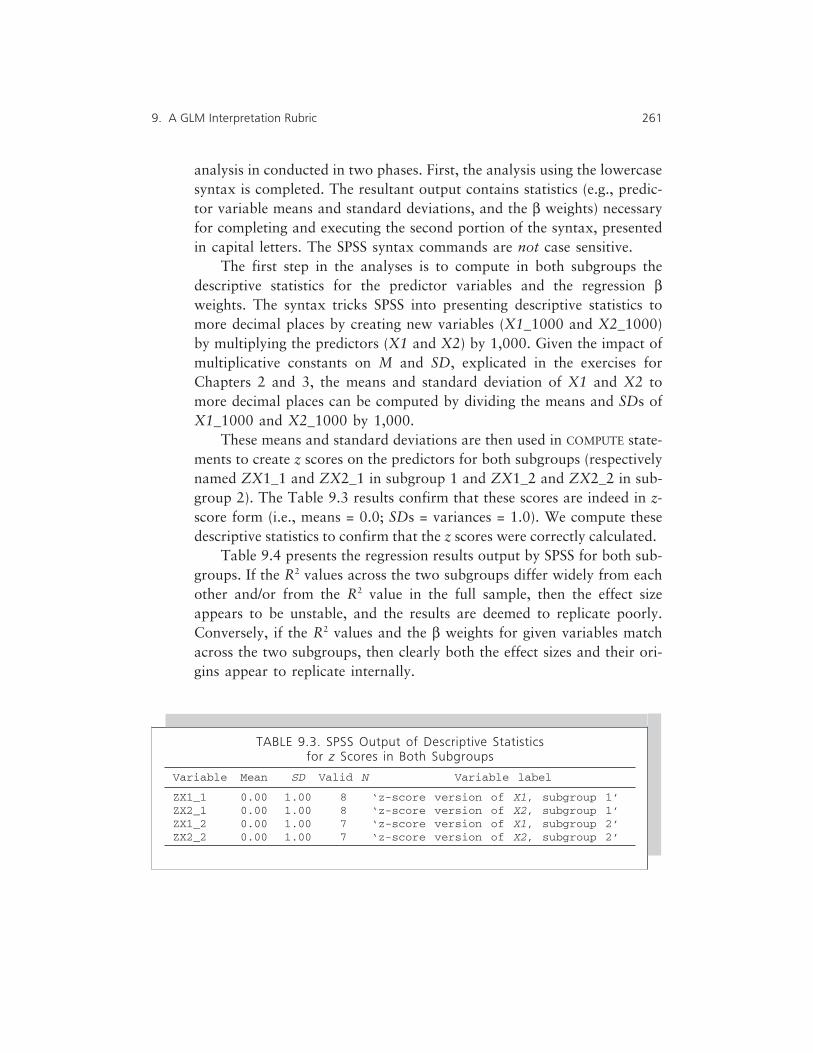
analysis in conducted in two phases. First, the analysis using the lowercasesyntax is completed. The resultant output contains statistics (e.g., predic-tor variable means and standard deviations, and the β weights) necessaryfor completing and executing the second portion of the syntax, presentedin capital letters. The SPSS syntax commands are not case sensitive.

The first step in the analyses is to compute in both subgroups thedescriptive statistics for the predictor variables and the regression βweights. The syntax tricks SPSS into presenting descriptive statistics tomore decimal places by creating new variables (X1_1000 and X2_1000)by multiplying the predictors (X1 and X2) by 1,000. Given the impact ofmultiplicative constants on M and SD, explicated in the exercises forChapters 2 and 3, the means and standard deviation of X1 and X2 tomore decimal places can be computed by dividing the means and SDs ofX1_1000 and X2_1000 by 1,000.

These means and standard deviations are then used in COMPUTE state-ments to create z scores on the predictors for both subgroups (respectivelynamed ZX1_1 and ZX2_1 in subgroup 1 and ZX1_2 and ZX2_2 in sub-group 2). The Table 9.3 results confirm that these scores are indeed in z-score form (i.e., means = 0.0; SDs = variances = 1.0). We compute thesedescriptive statistics to confirm that the z scores were correctly calculated.

Table 9.4 presents the regression results output by SPSS for both sub-groups. If the R2 values across the two subgroups differ widely from eachother and/or from the R2 value in the full sample, then the effect sizeappears to be unstable, and the results are deemed to replicate poorly.Conversely, if the R2 values and the β weights for given variables matchacross the two subgroups, then clearly both the effect sizes and their ori-gins appear to replicate internally.


TABLE 9.3. SPSS Output of Descriptive Statisticsfor z Scores in Both Subgroups

Variable Mean SD Valid N Variable label

ZX1_1 0.00 1.00 8 ‘z-score version of X1, subgroup 1’ZX2_1 0.00 1.00 8 ‘z-score version of X2, subgroup 1’ZX1_2 0.00 1.00 7 ‘z-score version of X1, subgroup 2’ZX2_2 0.00 1.00 7 ‘z-score version of X2, subgroup 2’

However, if the R2 values are comparable, but the β weights differacross the subgroups, our work is not yet done. We must conduct furtherempirical analyses to investigate whether the β weights are different, butstill yield reasonably comparable �Y scores across the two subgroups.

Cliff (1987, pp. 177–178) suggested that such cases involve “insensi-tivity” of the weights. For example, if all the predictors were highly, posi-tively correlated with each other and with the dependent variable, any onepredictor could arbitrarily be given a β weight of roughly 1, while theother variables would arbitrarily be given weights of roughly 0. All of thevarious possible combinations of a single β weight of 1 with severalweights of 0 might appear different in the subjective judgment of theresearcher, but would yield essentially equivalent �Y scores.

So, what is the same is the same. But what appears to be different maybe the same (i.e., still yield roughly equivalent prediction). In the lattercase, empirical analysis informs judgment as to whether apparent differ-ences in the β weights are meaningless, or they are noteworthy.

As reflected in the Figure 9.1 SPSS syntax, the empirical analysis isconducted as follows:

1. The predicted outcome scores for subgroup 1 are computed usingsubgroup 1’s data (the first number in the variable name) and βweights (the second number in the variable name; here YHAT11with n1 = 8).

2. The predicted outcome scores for subgroup 2 are computed usingsubgroup 2’s data and β weights (here YHAT22 with n2 = 7).


TABLE 9.4. SPSS Subgroup Regression Coefficientsfor the Figure 9.1 Syntax

Subgroup

Statistic n1 = 8 n1 = 7

Multiple R 0.73948 0.95729R Square 0.54683 0.91641Adjusted R Square 0.36556 0.87462β1 0.719003 0.920505β2 0.085253 0.078289

3. The predicted outcome scores for subgroup 1 are computed usingsubgroup 1’s data and subgroup 2’s β weights (here YHAT12 withn1 = 8).

4. The predicted outcome scores for subgroup 2 are computed usingsubgroup 2’s data and subgroup 1’s β weights (here YHAT21 withn2 = 7).

The 10 Pearson product–moment correlations of these four variables andthe Yi scores are then computed, as reported in Table 9.5.

Note that we are invoking β weights from the standardized scoreworld, but we are using Y scores from the unstandardized score world. Inthe present application, this is inconsequential. The �Y scores from the stan-dardized and the unstandardized worlds are always perfectly correlated,because additive and multiplicative weights do not affect r, as we learnedin the Reflection Problems of Chapter 5. For the same reason, the r of theYi scores and the �Y scores from the unstandardized score world always


TABLE 9.5. SPSS Output of Pearson r Coefficients

Note. The ns are presented in parentheses.aThese are the multiple correlation coefficients (R) in the two subgroups.bThese are the “shrunken” multiple correlation coefficients (R) in the two subgroups (e.g.,0.9573 to 0.9569). The shrinkage equals the difference in the R2 versus the shrunken R2 (e.g.,0.95732 – 0.95692 = 0.9164 – 0.9156 = 0.0008). The proportion of the shrinkage can beexpressed as 0.0008 / 0.9164 = 0.0009 = 0.09%.cThese are the invariance coefficients in the two subgroups, correlating the true �Y scores in agiven subgroup with the �Y scores computed using the weights from the opposite subgroup.

equals the r of the zY scores and the �Y scores from the standardized scoreworld.

Two of these rs in Table 9.5 are actually multiple correlation coeffi-cients (Rs). First, the rY × YHAT11 in subgroup 1 (n1 = 8) equals subgroup 1’sRY with X1, X2 (n1 = 8); as reported in Table 9.5, rY × YHAT11 = 0.7395, and inTable 9.4, RY with X1, X2 = 0.73948, respectively. Second, the rY × YHAT22 in sub-group 2 (n2 = 7) equals subgroup 2’s RY with X1, X2 (n2 = 7); as reported inTable 9.5, rY × YHAT22 = 0.9573, and in Table 9.4, RY with X1, X2 = 0.95729,respectively. These comparisons are important from both a conceptualand a practical point of view.

Conceptually, the recognition that a bivariate

rY × Y = RY × X1, X2 . . . (9.3)

and equivalently that

rY × Y2 = RY × X1, X2 . . .

2 (9.4)

suggests the very important concept that analyses really focus on latentvariables, and so the structure of the �Y scores must be an important ele-ment in result interpretation. The equality also suggests another way ofthinking about the �Y scores. The �Y scores are the useful information (i.e.,SOS) in the predictor variables, discarding all of and only the useless por-tion of the predictors that are not helpful in predicting Yi. Because theanalysis focuses on the criterion variable, and predicting informationabout the amount and origins of differences on Y, predictors are notewor-thy only to the derivative extent that the predictors in some way explain orpredict the Yi scores, and SOSY.

Practically, the comparisons of these two pairs of r and R coefficientsare important in testing whether the analysis has been properly conducted.If these two sets of coefficients do not match, we have made an error inour syntax, and must fix the error before proceeding further.

Next, we can compare in subgroup 1 (n1 = 8) the rY × YHAT11 = 0.7395(the real RY with X1, X2 in subgroup 1) with the rY × YHAT12 = 0.7391 (the empiri-cally-estimated “shrunken” R when we use subgroup 2’s weights withsubgroup 1’s data). Of course, if we want to calculate the exact shrinkage,


we must “square, before you compare” (i.e., shrinkage = 0.73952 –0.73912 = 0.54686 – 0.54627 = 0.00059). We can perform analogouscomparisons with subgroup 2’s results (i.e., n2 = 7, rY × YHAT11 = 0.9573, andrY × YHAT12 = 0.9569).

These two comparisons allow judgment about the internalreplicability evidence. When the amount of shrinkage in both subgroups issmall, as is the case here, some evidence is produced that results may bereplicable. This evaluation does not invoke a statistical significance test.

However, there is one complication. A small amount of shrinkagewhen the original effect size is small may be devastating, whereas a fairlylarge shrinkage in the presence of a huge initial effect size may still be tol-erable.

A context-free evaluation of replicability can be estimated by comput-ing an invariance coefficient to quantify the degree to which the �Y scoresare stable across resampling. We compute rYHAT11 × YHAT12 = 0.9995 andrYHAT22 × YHAT21 = 0.9996. We evaluate these coefficients against the hopethat the invariance coefficients will both approach +1.0. This is ourdesired value for the invariance coefficients regardless of the initial effectsize estimate.

However, three precepts must be considered in conducting cross-validation analyses. First, the subgroup analyses are conducted only toderive some empirical estimate of result stability, and are not used to esti-mate either the effect size or from where the effect originates. The fullsample results are always used as the basis for these interpretations,because the full sample has the largest n and therefore should yield themost accurate statistics.

Second, our expectations are that (a) the invariance coefficients willboth be large and (b) the invariance coefficients will be consistent acrossthe double cross-validation. Of course, these evaluations are more rigor-ous when the dfERROR is larger in both subgroups, because the models aremore falsifiable in such situations.

Third, bear in mind that the number of possible random sample splitscan be quite large, when n is reasonably large. And different sample splitsmay yield divergent invariance coefficients for the same data. Thus, cross-validation methods must be interpreted cautiously. The methods have theadvantage that specialized software is not required (and that performing


these calculations also heuristically leads to greater understanding oflatent variables and of multiple correlation). And although the methodsare limited, they are considerably more useful than incorrectly NHSST assome kind of internal replicability evidence.

�� Where Does My Something Originate?

If our answer to our first question, “Do I have anything?” is no, then ourresult interpretation obligations have been met, and we are done withexamining the statistical results. Only a fool would ask, “From where doesmy nothing originate?” or “Which predictors contribute most to predict-ing nothing?” Conversely, iff we answer yes, based on whatever combina-tion of the three facets of evidence we decide to evaluate, then we mustaddress the question, “From where does my noteworthy effect originate?”

Logically, the b or the β weights might be consulted to address thissecond question. After all, the b and the β weights are used to compute the�Y scores, which are a primary focus of the analysis. And the structure coef-ficients (rS) provide insight into the nature of the �Y scores, so these coeffi-cients also seem important in addressing this second question.

As noted in Chapter 8, in Case #1, we can formulate our answer byevaluating (a) the β weights, or (b) the r between the Yi scores and eachpredictor, or (c) the r between the �Y i scores and each predictor (i.e., eachrS). In Case #1, for a given predictor β = rY × X. Also, in a given analysis, therS values will always be proportional to the corresponding β weights (andthe corresponding r of Y with a given predictor) because

rS = rX with Y / R (8.14)

The rs between predictors and the Yi scores are simply scaled in a differentmetric than the rs between predictors and the �Y i scores, by a factor of R.And in Case #1, iff R = 1.0, for a given predictor β = rX with Y = rS.

So, in Case #1, only one set of coefficients must be consulted to com-plete result interpretation. In Cases #2 or #3, two sets of coefficients mustbe simultaneously considered.


Weights

Given that multiplicative weights ought to be consulted in addressing theorigins of detected effects, why are the b weights usually not used as thebasis for interpretation? As explained in Chapter 8, a given b weight isjointly influenced by (a) the uniquely credited power of X scores in thegiven research context to help predict, either directly or indirectly, the Yi

scores, and (b) the standard deviations of the predictor variable in relationto the SDY.

Because the b weights are a confounded function of these two dynam-ics, five predictors could all have b weights of +2.5, but each differ in theirpredictive contributions in the context of these five predictors. Or the pre-dictor with the b weight closest to zero may actually be the best predictorin the context of the predictor variable set.

The β weights are applied to the predictors in z-score form in the stan-dardized score world. Because the standard deviations of the predictorshave been removed by division when computing the z scores, the β weightsare only influenced by the uniquely credited power of zX scores in thegiven research context to help predict, either directly or indirectly, the zY

scores. Thus, in a given research context the β weights can be compared toeach other apples to apples.

However, because

b = β(SDY / SDX) (8.1)

if all the predictors have the same SD, then the set of b and the set of βweights will be proportional to each other. And when all the measuredvariables, including the Y variable, have the same SD, then the b and the βfor given predictors will be equal.

Therefore, b weights can be used in result interpretation when the pre-dictor variables all have the same SD. For example, in their study Glaser,Hojat, Veloski, Blacklow, and Goepp (1992) correctly interpreted bweights rather than β weights, noting that,

As the MCAT subtests are all reported on the same standardized scale(Mean = 8, SD = 2) one may use the magnitude of the obtained (non-standardized) regression coefficients (b-values reported in the table) to deter-


mine the relative importance of the contribution of each predictor in theregression models. (p. 399)

But equality of predictor SDs occurs rarely, and so β weights are usu-ally one focus in evaluating result origins. The a and b weights are primar-ily useful in predictive applications of regression, where we focus on the �Y i

scores in the unstandardized score world (e.g., predicted height of childrenin inches once adult) rather than estimates of standardized z-score height,because z scores are seen as being less friendly by the nonstatisticians usu-ally involved in predictive situations.

Four precepts should govern the interpretation of the β weights. First,typically, the signs of the β weights are irrelevant, except that the contextof a given scaling decision must be considered. The signs of the β weightsare usually arbitrary because in the social sciences the scaling direction ofour measures is usually arbitrary. We can score an academic test by count-ing the number of right answers, or the number of wrong answers. Ineither case, we are measuring the same construct.

Second, remember that β are only bivariate correlation coefficients inCase #1. So do not use the word “correlation” in the context of the βweights unless you are in Case #1. But in all cases, a β weight indicates thepredicted number of SD units of change in the �Y i scores for 1 standarddeviation of change on a given predictor, given the context of a particularset of predictors. For example, if the predictor is the number of rightanswers on an academic test, and β = +2.5, this means that for 1 SDX ofimprovement on scores on the test, the �Y i scores are predicted to improveby 2.5 SDYs, holding all other scores constant, and in the context of agiven set of predictors.

Third, as repeatedly emphasized in Chapter 8, remember that βweights are context specific. If you add a single predictor to the model, orremove a single predictor, all the β weights could fluctuate wildly, unlessyou are in Case #1. In Cases #2 and #3, this implies that caution must beexercised when interpreting the β weights, unless you are somehow certainthe model is correctly specified.

Fourth, use caution when interpreting NHSST for the multiplicativeweights. The pCALCULATED values for a given pair of b and β weights in agiven study are identical. But remember that all tests of statistical signifi-cance, including the test of H0: b (or β) = 0, are driven by sample size (see


Ziliak & McCloskey, 2004). This means that an identical set of β weightsmay all be statistically significant in one study with a large n, whereasnone are statistically significant in another study with a smaller n.

Structure Coefficients

When b = 0.0, β = 0.0, and vice versa, and the multiplicative weight oblit-erates the predictor variable. In Case #1, a predictor with β (and b) = 0.0 isdefinitively useless. The predictor cannot help, either directly (by predict-ing variability in the Yi scores) or indirectly (by making one or more otherpredictors better predictors of the Yi scores), to explain the SOSY.

But in Case #2, a predictor with a zero β weight might, in fact, be thesingle best predictor in the predictor variable set. The predictor may sim-ply be denied any predictive credit for commonly explained Yi score vari-ability also explained by other correlated predictors. In such a case, thepredictor would have a large rS

2.And in Case #3, a predictor might have rS

2 (and rS) of zero, but also aβ weight largest in absolute magnitude among the weights for the predic-tor set. In such a situation, we know definitively that the predictor is asuppressor variable.

Across all cases, only when a given predictor has both β = 0.0 and rS =0.0 is the predictor completely useless, at least in the context of a given setof predictors. Clearly, as Courville and Thompson (2001) and others (e.g.,Dunlap & Landis, 1998; Thompson & Borrello, 1985) have argued, “β is[often] not enough.”

Of course, as noted previously, because the rs between the predictorsand the Yi scores are proportional to the corresponding rs between the pre-dictors and the �Y i scores, the same interpretations across all three regres-sion cases would be realized by consulting the rs between the predictorsand the Yi scores. The selection of a supplement to the interpretation ofthe β weights across the two choices is entirely stylistic.

Unhappily, empirical studies (e.g., Courville & Thompson, 2001) ofpublished regression research show that researchers invariably interpretonly β weights. The consequence is gross misinterpretation of results inmuch of the literature.

An emphasis on regression structure coefficients is also consistent


with the emphasis on rS throughout the general linear model, where forsome reason the rSs (unlike the weights) are always called the same thing(i.e., structure coefficients). For example, structure coefficients are deemedcritical to result interpretation in both exploratory (cf. Gorsuch, 1983,p. 207; Thompson, 2004) and confirmatory (cf. Graham, Guthrie, &Thompson, 2003) factor analysis.

The same is true in descriptive discriminant analysis (cf. Huberty,1994, p. 206) and canonical correlation analysis (cf. Levine, 1977, p. 20).Thus, Meredith (1964, p. 55) suggested, “If the variables within each setare moderately intercorrelated the possibility of interpreting the canonicalvariates by inspection of [only] the appropriate regression weights [func-tion coefficients] is practically nil.”

�� Stepwise Methods

In some predictive applications, researchers have access to a large numberof predictor variables, and conduct a specification search (i.e., change themodel specification) by looking for a more parsimonious, smaller subsetof predictors that may be almost as effective as the full set of predictors inyielding accurate �Y i scores. Some researchers attempt to invoke what arecalled stepwise methods for this purpose. Huberty (1994) has noted, “It isquite common to find the use of ‘stepwise analyses’ reported in empiricallybased journal articles” (p. 261).

Stepwise analysis is a forward or a backward progression in whichpredictor variables are added or deleted from the model one variable at atime, based atheoretically on empirical analyses of the sample data. Theforward progression is more commonly encountered than is backwardanalysis.

In forward stepwise regression, software first computes the bivariater2 values between each predictor variable and the Yi scores. The predictorwith the largest r2 with Y is entered in the first step. The selection by step-wise of the best single predictor is correct.

In the second step, the remaining predictors are evaluated to deter-mine which one predictor, when added to the model, will yield the largestincrease in R2, in the context of the first predictor’s presence in the model.


Thus, a predictor that is very highly correlated with the first-entered pre-dictor may never be entered into the model, even if this predictor is thesecond-best single predictor in the predictor variable set.

In the third step, the remaining predictors are evaluated to determinewhich one predictor, when added to the model, will yield the largestincrease in R2, in the context of the first two predictors’ presence in themodel. The process continues by considering the addition of remainingpredictors.

However, next and after all the remaining steps, the removal of previ-ously-entered predictors is also considered. For example, in the presenceof three predictors, if the first predictor’s explanatory power is present inthe second and third predictors selected, then the first predictor will beremoved from the model.

As programmed in commonly-used statistical packages, the forwardselection procedure continues until the change in R2 from one step versusthe R2 in the immediately previous step is no longer statistically signifi-cantly different from zero. In any context, including stepwise, we can testthe null that H0: RLARGER

2 = RSMALLER2 (or H0: RLARGER

2 – RSMALLER2 = 0) using

the generic equation:

FCALCULATED = [(RLARGER2 – RSMALLER

2) / (kL – kS)] / (9.5)[(1 – RLARGER

2) / (n – kL – 1)]

where kL is the number of predictors used to obtain RLARGER2, and kS is the

number of predictors used to obtain RSMALLER2. The df are (kL – kS) for the

numerator, and (n – kL – 1) for the denominator.In stepwise, kL – kS equals 1 at each successive step, so Equation 9.5

simplifies in this application to

FCALCULATED = [RLARGER2 – RSMALLER

2] / [(1 – RLARGER2) / (n – 2)] (9.6)

In this application, the degrees of freedom are 1 for the numerator and(n – kL – 1) for the denominator. Of course, this means that 100 research-ers evaluating the same ∆R2 (i.e., RLARGER

2 – RSMALLER2) for the same number

of steps, but with 100 different sample sizes, will each obtain differentpCALCULATED values, and some may make different decisions, even at a fixedα about when to discontinue the stepwise analysis.


Three Problems

There are three primary problems with stepwise analyses (Thompson,1995). Various scholars have noted these problems (e.g., Huberty, 1989;Snyder, 1991; Thompson, 2001) and suggested that stepwise methodsshould never be used. Indeed, one article in this venue was entitled “WhyWon’t Stepwise Methods Die?” (Thompson, 1989b).

Wrong Degrees of Freedom

Commonly-used statistical packages incorrectly compute the FCALCULATED

and pCALCULATED used to test the final R2 evaluated at the conclusion of thestepwise analysis, because the wrong degrees of freedom are used. ThedfTOTAL is correctly computed as n – 1. However, the dfREGRESSION is com-puted as the number of variables that stepwise has entered, and thedfRESIDUAL is computed as dfTOTAL minus this dfREGRESSION. Instead, thedfREGRESSION should be the number of predictor variables in the study.

The dfREGRESSION are the coins we spend to ask questions of our data.We can enter into a model no more than dfTOTAL predictor variables (andshould enter considerably fewer predictors, so that dfRESIDUAL ≠ 0, and themodel remains falsifiable).

Software should charge us for 1 degree of freedom for every predictor“tasted,” regardless of how many predictors are ultimately retained in theanalysis. As Thompson (2001) observed,

This is bad behavior. The movie I show my students to teach them that this isbad behavior is “Animal House” when John Belushi is in the student cafete-ria. He tastes all the entries on the buffet line, but doesn’t pay for the items hetasted and put back (or stuffed in his pockets). My students, who includesome serious cafeteria experts, assure me that this behavior would not be tol-erated at many of your finer cafeterias. Nor should such [bad] behavior betolerated in statistics. (p. 87)

Note that if 5 out of 50 predictors were selected randomly, or based onprior findings, or theory, and all 50 predictors were not tasted by stepwise,then dfREGRESSION = 5 would indeed be entirely correct.

Table 9.6 illustrates the impacts for a hypothetical situation involving


n = 126, 5 steps of forward stepwise with a pool of 50 predictor variables,and an R2 of 10.00%. For the incorrect degrees of freedom, pCALCULATED is0.025, and so the result is statistically significant at α = 0.05. But when thecorrect degrees of freedom are computed, FCALCULATED is less than 1 and socannot be statistically significant even at infinite degrees of freedom. Here,for the correct degrees of freedom, the Excel =FDIST statistical functioncalculates that pCALCULATED = 1.00, and the result is not statistically signifi-cant.

Of course, this problem is not inherent in stepwise methods, butinstead is a flaw in the statistical software implementations of these meth-ods. The consequence of using a deflated dfREGRESSION along with an inflateddfRESIDUAL is typically a “double whammy” inflation of FCALCULATED and acorresponding “double whammy” deflation of pCALCULATED. Thus, Cliff(1987, p. 185) noted that “most computer programs for [stepwise] multi-ple regression are positively satanic in their temptations toward Type Ierrors.”

The problem may be less acute when sample size is (a) extraordinarilylarge and the number of predictor variables is very small or (b) the final R2

is small. In these cases, the differences in the correct and incorrectpCALCULATED values will not be as large, as could be seen by modeling varia-tions on the Table 9.6 results for various ns, numbers of predictors, andeffect sizes. Nevertheless, in all cases, the computer packages use the incor-rect degrees of freedom, and the only question is how wrong the incorrectresults are.


TABLE 9.6. Stepwise NHSST for Hypothetical Example

Analysis/source SOS df MS FCALCULATED pCALCULATED R2

IncorrectRegression 10.0 5 2.00 2.667 0.025 10.00%Residual 90.0 120 0.75Total 100.0 125 0.80

CorrectRegression 10.0 50 0.20 0.167 1.000 10.00%Residual 90.0 75 1.20Total 100.0 125 0.80

Capitalization on Sampling Error

All samples include variance that mirrors true variance in the population,as well as idiosyncratic variance unique to the sample (i.e., sampling errorvariance). Unfortunately, in stepwise even a very small amount of sam-pling error variance can result in an incorrect predictor selection decision(i.e., a decision that would not occur if stepwise for the same variables wasperformed in the population).

Furthermore, stepwise makes a linear sequence of entry decisions. Amistake at any step impacts and potentially compromises all subsequententry decisions. Because in stepwise an infinitesimal competitive advan-tage for entering a predictor will result in that variable’s selection, andthat infinitesimal advantage may be due to sampling error, and also preju-dice subsequent decisions, “a large proportion of the published resultsusing this method probably present conclusions that are not supported bythe data” (Cliff, 1987, pp. 120–121).

For example, if for an analysis involving 50 predictors, the bestsingle predictor rY × X

2 = 10.0001%, and for a second predictorrY × X

2 = 10.0000%, the first predictor will be entered before the secondvariable, and the second variable may never get entered. Of course, thisproblem is partly a function of collinearity, and is less severe as theresearch approaches Case #1. On the other hand, in Case #1, the step-wise predictor variable entry order will exactly correspond to thesquared correlations of the predictors with the Yi scores, so stepwise inCase #1 represents an uninteresting situation in which no researcherwould use stepwise.

Freedman (1983) conducted a Monte Carlo simulation study demon-strating that even if we sample from a population in which the predictorseach have no relationship with Y, a large sample R2 will result. Hereported:

To focus on an extreme case, suppose that in fact there is no relationshipbetween the dependent variable and the explanatory variables. Even so, ifthere are many explanatory variables, the R2 [from a stepwise analysis] willbe high. . . . This is demonstrated [here] by simulation and by asymptotic cal-culation. (p. 152)


R2 Not Optimized

Some researchers erroneously believe that stepwise methods identify theset of predictors of size k that will yield the largest R2 given the use of kpredictors with the dataset (Huberty, 1989, p. 45). To the contrary, (a)another combination of k predictors may yield a larger R2 than the R2 forthe k predictors picked by stepwise, and furthermore (b) the best set of kpredictors might not include any of the k predictors selected by stepwise(see Thompson, 1995)!

Equating stepwise with finding the optimal set of k predictors is illogi-cal, because stepwise and finding the best set of k predictors involve twodifferent questions. In an analogy to selecting five players on a basketballteam, stepwise sequentially asks, “In a given selection, which one playershould I add to the team, given the previous players selected?”

Conversely, the correct selection method would ask, “For all possibleteams of five players, which team plays the best?” The best team of fivemay not be the team identified via a sequence of selections, because askinga question about team quality does not raise any issues of incrementalselection, and incremental selection issues are completely irrelevant toselecting the best team.

The only way to select the best possible team of basketball playersfrom a pool of 50 players is to evaluate all possible teams of 5. The bestteam might not include the players picked in a stepwise algorithm. Andthe best team of 5 might not even include the single best player, when thebest player does not play well with others. By the same token, the onlytime that stepwise picks the best predictor variable set of size k is in Case#1, which is not a situation in which stepwise is likely to be used, becausehere in the presence of all the rY × X

2 values, no value is added by conduct-ing the stepwise analysis.

Alternative Models

Two alternative models to stepwise, unlike stepwise, may be very useful inresearch. The two models involve hierarchical and all-possible-subsetsanalyses, respectively.

However, it is important to realize that regardless of the model (e.g.,


stepwise, hierarchical, all-possible subsets) used, once a given set of k pre-dictors is identified, the β weights and the structure coefficients for thesepredictors will be the same no matter how the k predictors are identified.So, with a given set of k = 5 predictors, if β1 = –2.80, and rS for the firstpredictor is –0.75, β1 will equal –2.80 and rS will equal –0.75 if stepwisewas used, or the five predictors were selected using darts, or tarot cards, orall-possible-subsets analyses, or any method.

Hierarchical Entry

Hierarchical predictor variable entry involves entering predictors in prede-termined blocks (e.g., using a series of ENTER subcommands within theSPSS REGRESSION procedure) based on theory or previous research. Thus,the data are not consulted in selecting the blocks or their order entries.

For example, if a researcher had variables measured at birth (i.e., X1,X2, and X3), variables measured in first grade (e.g., F1, and F2), and vari-ables measured in sixth grade (e.g., S1, S2, and S3), the variables mightlogically be entered in three blocks reflecting the chronology of measure-ment. This could be accomplished in SPSS by invoking the subcommandsyntax within REGRESSION:

ENTER x1 x2 x3/ENTER f1 f2/enter s1 s2 s3

At each block of variable entry, an R2 will be printed. For a givendataset with a fixed n, the uncorrected R2 can never become smaller asmore measured predictors are used. Of course, the uncorrected R2 couldtheoretically remain unchanged as more predictors are added, and the cor-rected R2 could get smaller. Also, if desired, the statistical significance ofthe differences in the sequential R2 values could be evaluated with Equa-tion 9.5.

Hierarchical entry is theory-driven, and can be used to address inter-esting theoretical propositions, such as developmental models. For exam-ple, in the illustrative situation described here, we may use these models totest whether education after first grade has any impacts beyond those pres-ent in first grade.


All-Possible-Subsets Analysis

In predictive applications, the researcher may seek a more parsimonious(smaller) set of predictors that may still yield an acceptable R2, or even anR2 that is roughly comparable to the effect size obtained from using thefull pool of predictors. However, as suggested previously, stepwise is notsuitable for this (or any other) purpose.

The correct selection method begins by computing the R2 for each andevery combination of predictors for each and every variable set size. Thecomputations sound daunting but, actually, can be painlessly performedby some software in only moments.

Figure 9.2 presents a line plot of the maximum R2 values for a givennumber of k predictors. This plot can be consulted to inform theresearcher’s subjective judgment regarding the optimal number of predic-tors to retain. In this example, the plot seems to level off after the predic-tor variable set size is k = 5 (R2 = 57.1% with k = 5, versus R2 = 58.1%with k = 6).

If the ~57.1% effect size is deemed sufficient, given the researcher’spredictive application, the focus then turns to which five predictors shouldbe retained for future use. Thoughtful researchers will look at several R2

values for k = 5, and then thoughtfully select the predictor variable set atk = 5 with variables that can be most easily or most cheaply measured. Ak = 5 variable set with a slightly less-than-optimal effect size might be pre-ferred for practical reasons.

A variant on this all-possible-subsets analysis would instead plot“adjusted R2” values. This alternative will be most appealing when sam-


FIGURE 9.2. Line plot of successive R2 values

pling error variance is likely to be larger, as when sample size is relativelysmall.

�� Invoking Some Alternative Models

Various interesting alternative or complementary regression models maybe helpful in some research situations. Four particularly noteworthy mod-els are considered here: (a) commonality analysis, (b) path analysis, (c)curvilinear regression invoking predictors taken to various exponentialpowers to model curvilinear relationships, and (d) testing interactioneffects.

Commonality Analysis

Commonality analysis (Beaton, 1973; Mood, 1969; Seibold & McPhee,1979; Thompson, 1985) can be used to decompose either the R2 or theSOSEXPLAINED into constituent, nonoverlapping parts that involve theunique and the common explanatory powers of the predictors (or sets ofpredictors) in all their possible combinations. For example, in the contextof two predictors (or two sets of predictors, each involving one or morevariables), we could ask, (a) How much explanatory power is unique tothe first predictor (or predictor set)? (b) How much explanatory power isunique to the second predictor (or predictor set)? and (c) How muchexplanatory power is common to both predictors (or predictor sets) andcould be derived from either predictor (or predictor set)?

Rowell (1996) presented an accessible treatment of these methods.Table 9.7 presents the formulas that can be used to derive these estimatesfor either two, three, or four predictor variables (or predictor variablesets). Formulas for more predictors can be found elsewhere (e.g., Rowell,1996).

Commonality analysis is only of potential interest in either Case #2 orCase #3. In Case #1, because all the predictor variables are uncorrelated,(a) there is no common explanatory power of the predictors acting in con-cert in sets of two or more, and (b) all the unique explanatory power of agiven predictor is quantified by the r2 of the given predictor with the Yi

scores.


To make this discussion concrete, let’s consider the prediction oflibrary users’ ratings (n = 69,358) of library service quality using theLibQUAL+TM protocol (Thompson, Cook, & Heath, 2003a, 2003b), pre-dicted by (a) global library satisfaction scores, (b) global scores on aca-demic outcomes facilitated by the library, and (c) frequency of library usescores. The necessary results to apply the Table 9.7 equations are pre-sented in Table 9.8.

The Table 9.8 results can easily be plugged into a spreadsheet pro-gram to produce the output reported in Table 9.9. Note that the unique


TABLE 9.7. Formulas for Uniqueand Commonality Components of Shared Variance

and the common explanatory partitions of the R2 (i.e., 58.698%) for agiven variable sum together to equal the r2 of a given predictor with the Yi

scores (e.g., UniqueSATISFACTION + CommonSATISFACTION with OUTCOMES and USE =rSATISFACTION with LibQUAL+(TM) = 19.409% + 37.587% = 56.996%).

It is also noteworthy that the sum of all seven nonoverlapping parti-tions of R2 equals the R2 of the three predictors with the LibQUAL+TM

scores. Thus, 19.409% + 1.684% + 0.032% + 37.488% + –0.023% +–0.014% + 0.122% = 58.698%. This merely reiterates the truism thatcommonality here is being used to partition the R2 into (seven) constitu-ent, nonoverlapping parts.

Some comment on the negative variance partitions is necessary.Clearly, negative variances are troubling because, as area-world statistics,variances theoretically have a minimum value of zero. Traditionally, near-zero values in commonality analyses are treated as zeroes. If some negativevalues are large, the possibilities of model misspecification, or of suppres-sor effects, are suggested, and the results would be deemed not reasonable.

Commonality analysis can also be used to partition the SOSEXPLAINED

(here 56,983.94). The analysis is performed by multiplying the Table 9.9results by the SOSEXPLAINED of 56,983.94, again using a spreadsheet. Theresult is presented in Table 9.10.

In the present example, the commonality analysis can be used to helpus understand what the LibQUAL+TM scores measure. Several conclusionsare suggested.

First, the LibQUAL+TM scores appear insensitive to frequency of


TABLE 9.8. Coefficients Required for the Table 9.7 Computations

Predictors r2 or R2

Satisfaction 56.996%Outcomes 39.280%Use 0.117%Satisfaction, Outcomes 58.666%Satisfaction, Use 57.014%Outcomes, Use 39.289%Satisfaction, Outcomes, Use 58.698%

library use. Frequency of library use either alone (UniqueUSE = 0.032%) orin concert with either or both of the other predictors (CommonUSE =0.085%) contributes little to defining R2 = 56.996%.

Second, academic outcomes explain about two-thirds of the R2 =58.698% (i.e., r2

LibQUAL+(TM) with OUTCOMES = 39.280% / 58.698% = 0.669), butgiven that most of this overlaps with the other two predictors (i.e.,CommonOUTCOMES = 37.596% / 39.280% = 0.957), the outcomes scores


TABLE 9.9. Unique and Common Components of Shared Variance (R2)

Predictors

Predictors/partitions Satisfaction Outcomes Use

Satisfaction 19.409%Outcomes 1.684%Use 0.032%Satisfaction, Outcomes 37.488% 37.488%Satisfaction, Use –0.023% –0.023%Outcomes, Use –0.014% –0.014%Satisfaction, Outcomes, Use 0.122% 0.122% 0.122%

Unique 19.409% 1.684% 0.032%Common 37.587% 37.596% 0.085%Total 56.996% 39.280% 0.117%

TABLE 9.10. Sum-of-Squares (SOS) Explained by Predictor Sets

Predictors

Predictors Satisfaction Outcomes Use Cumulation

Satisfaction 18842.23 18842.23Outcomes 1634.82 1634.82Use 31.07 31.07Satisfaction, Outcomes 36393.30 36393.30 36393.30Satisfaction, Use –22.33 –22.33 –22.33Outcomes, Use –13.59 –13.59 –13.59Satisfaction, Outcomes, Use 118.44 118.44 118.44 118.44

Total 56983.94

contribute little to predicting the LibQUAL+TM scores in the presence ofthe other scores.

The satisfaction scores uniquely contribute about one-third of theR2 = 58.698% (i.e., 19.409% / 58.698% = 0.331). And the satisfactionand outcomes scores as a predictor pair have in common the capacity toexplain about two-thirds of the R2 = 58.698% (i.e., 37.488% / 58.698% =0.639). The remaining five variance partitions are all quite small, the larg-est being only UniqueOUTCOMES = 1.684%. Clearly, in the context of thispredictor variable set, the LibQUAL+TM scores must be considered basi-cally a global measure of patron satisfaction with libraries.

Path Analysis

Path analysis was conceptualized by Sewall Wright (1921, 1934) as a wayof studying the direct and indirect impacts of measured variables on othermeasured variables considered to be effects. A brief treatment here is war-ranted for three reasons. First, like commonality analysis, path analysiscan be conceptualized as another way to decompose correlations. Thisprocess is fundamental to all data analysis, and so is important conceptu-ally to an understanding of what statistical analyses do. Second, the meth-ods can be substantively important in their own right.

Third, path analysis, when married with a multivariate techniquecalled confirmatory factor analysis (see Thompson, 2004), creates amethod called structural equation modeling (SEM). SEM is a very power-ful multivariate analysis, which is beyond the scope of the present book(see Thompson, 2000b, for an introductory explanation). Nevertheless,some understanding of path analysis will facilitate subsequent understand-ing of SEM, and path analysis is an important analytic method in its ownright.

The purpose of this brief discussion is not to make you an expert onpath analysis. The purpose is only to make you aware of additional ana-lytic possibilities, expose you to a few key concepts, and perhaps exciteyou to do some further reading.

To make this discussion concrete, consider the hypothetical data pre-sented in Table 9.11, which represent a variation on an example providedby Kerlinger and Pedhazur (1973, pp. 305–326). The example involves


prediction of GPA with socio-economic status (SES), psychological needfor achievement (nAch), and IQ scores (IQ).

The path model we will test is presented in Figure 9.3. In a real analy-sis, a critical feature of the investigation would involve laying out anempirical and/or theoretical justification for the model. Also, real analysesusually should test multiple rival models, because the fit of a preferredmodel to our data is more persuasive when the preferred model fits betterthan plausible rival models (Thompson, 2000b). Our model has beendrawn under the assumptions that (a) all relationships are linear, (b) allcausal flows are one way (i.e., there are no two variables linked by recip-rocal causation, or in other words, no two variables are linked by a pair ofone-headed arrows going in opposite directions), and (c) the measuredvariables are intervally-scaled.

We will analyze the measured variables in their z-score forms, andthus be estimating β weights, so that the weights can be compared witheach other apples-to-apples. In a path analysis diagram involving mea-sured variables in their z-score forms, two-headed arrows represent corre-


TABLE 9.11. Pearson r Matrix for Predicting GPA

Variable SES nAch IQ GPA

SES 1.000 0.250 0.510 0.351nAch 0.250 1.000 0.190 0.590IQ 0.510 0.190 1.000 0.510GPA 0.351 0.590 0.510 1.000

FIGURE 9.3. Path analysis model

lation coefficients. One-headed arrows involve estimates of pathcoefficients. We require an estimate of the coefficient implied by each ofthe six arrows in Figure 9.3.

Path Coefficient Estimation

The coefficient for the rSES × nAch two-headed arrow can be derived by insert-ing into the diagram the appropriate entry from Table 9.11 (i.e., r = 0.250= p1). To find the path coefficients for predicting IQ from SES, and IQfrom nAch, we conduct a regression predicting IQ with only SES andnACH. The resulting β weights provide these two path coefficients.

We can compute these β weights using Equations 8.12 and 8.13. ForSES predicting IQ within this model, we have

βSES = [rSES × IQ – {(rnAch × IQ)(rSES × nAch)}] / [1.0 – rSES × nAch2]

[0.510 – {(0.190)(0.250)}] / [1.000 – 0.2502][0.510 – {(0.190)(0.250)}] / [1.000 – 0.063]

[0.510 – {(0.190)(0.250)}] / 0.938[0.510 – 0.048] / 0.938

0.463 / 0.938= 0.493

Thus, p2 = βSES = 0.493.For nAch predicting IQ within this model, we have

βnAch = [rnAch × IQ – {(rSES × IQ)(rSES × nAch)}] / [1.0 – rSES × nAch2]

[0.190 – {(0.510)(0.250)}] / [1.000 – 0.2502][0.190 – {(0.510)(0.250)}] / [1.000 – 0.063]

[0.190 – {(0.510)(0.250)}] / 0.938[0.190 – 0.128] / 0.938

0.063 / 0.938= 0.067

Thus, p3 = βnAch = 0.067.Finally, to compute the p4, p5, and p6 coefficients, we perform a regres-

sion predicting GPA with SES, nAch, and IQ. We could do this simply byrunning the necessary regression in SPSS or another package. Alterna-


tively, we could obtain the same result by requiring SPSS to do the neces-sary calculations step by step, using the following syntax. In either case,when predicting GPA, we would obtain p4 = βSES = 0.018, p5 = βIQ = 0.404,and p6 = βnAch = 0.509.

Partitioning Direct and Indirect Effects

One way to interpret our results is by conceptualizing the model as pre-dicting changes in measured variables as a cumulation of direct and indi-


rect effects from changes in predictor variable scores. For our model, wehave

zSES = eSES,znAch = enAch,

zIQ = p2[zSES] + p3[znAch] + eIQ,zGPA = p4[zSES] + p6[znAch] + p2[zSES][p5] + p3[znAch][p5] + eGPA

where es are the error terms resulting whenever our model does not per-fectly fit our data.

The model can be used to estimate changes in an outcome associatedwith change in a predictor by a given number of standard deviation units,holding other measured variables constant. For example, if a given per-son’s nAch increased by 1 SD, the predicted change in IQ would be solelydue to direct effects of the change in nAch, and would be

zIQ = p2[zSES] + p3[znAch]

or

zIQ = 0.493[0] + 0.067[1]

or an increase of 0.067.However, if a given person’s nAch increased by 1 SD, the predicted

change in GPA would be impacted both directly and indirectly by thischange. The predicted change in GPA would be

zGPA = p4[zSES] + p6[znAch] + p2[zSES][p5] + p3[znAch][p5]

or

zGPA = 0.018[0] + 0.509[1] + 0.493[0][0.404] + 0.067[1][0.404]

or an increase of 0.509 (i.e., 0.509[1]) from the direct effects of the changein nAch, as well as an additional increase of 0.027 (i.e., 0.067[1][0.404])from the indirect effects of the change in nAch working through IQ.


Partitioning r2s and Evaluating Model Fit

The path coefficients can also be used to estimate the bivariate rs amongthe measured variables, or can be viewed as a decomposition of the esti-mated bivariate rs among the measured variables (see Loehlin, 2004,Ch. 1). This insight yields the conceptual understanding that the pathmodel is attempting to yield a matrix of estimated correlations that willapproximate the actual values in Table 9.11. Beyond the heuristic value ofcomparing estimated with actual r values, to emphasize that the model isan alternative representation of the correlations, from a practical stand-point we compare the reproduced or estimated correlations with ouractual correlations to help evaluate whether our model fits our data, andthe model seems reasonable. Here we can decompose the six unique corre-lation coefficients presented in Table 9.11.

First, given our coefficients, the rGPA × SES is estimated as

rGPA × SES = p4 + [(p6)(rSES × nACH)] + [(p5)(rIQ × SES)]0.017579 + [(0.508775)(0.250)] + [(0.404368)(0.510)]

0.017579 + 0.127193 + [(0.404368)(0.510)]0.017579 + 0.127193 + 0.206227

0.017579 + 0.333421rGPA × SES = 0.351000

Alternatively, we can decompose the correlation using only the path coeffi-cients from the path analysis. Now we have

rGPA × SES = [(p1)(p6)] + [(p1)(p3)(p5)] + [(p2)(p5)] + p4

[(0.250)(0.508775)] + [(0.250)(0.066667)(0.404368)] +[(0.493333)(0.404368) + 0.017579

0.127194 + 0.006740 + 0.199488 + 0.017579rGPA × SES = 0.351000

Second, rGPA × nACH is estimated as

rGPA × nACH = [(p4)(rSES × nACH)] + p6 + [(p5)(rIQ × nACH)][(0.017579)(0.250)] + 0.508775 + [(0.404368)(0.190)]

0.004394 + 0.508775 + [(0.404368)(0.19)]0.004394 + 0.508775 + 0.076829

0.004394 + 0.585604rGPA × nACH = 0.589999


Alternatively, using only the path coefficients, we have

rGPA × nACH = [(p1)(p4)] + [(p1)(p2)(p5)] + [(p3)(p5)] + p6

[(0.250)(0.017579)] + [(0.250)(0.493333)(0.404368)] +[(0.066667)(0.404368)] + 0.508775

0.004395 + 0.049872 + 0.026958 + 0.508775rGPA × nACH = 0.590000

Third, rGPA × IQ can be decomposed as

rGPA × IQ = [(p4)(rIQ × SES)] + [(p6)(rIQ × nACH)] + p5

[(0.017579)(0.510)] + [(0.508775)(0.190)] + 0.4043680.008965 + [(0.508775)(0.190)] + 0.404368

0.008965 + 0.096667 + 0.4043680.008965 + 0.501035rGPA × IQ = 0.510000

Using only the path coefficients from the path model, we have

rGPA × IQ = [(p2)(p1)(p6)] + [(p3)(p6)] + [(p2)(p4)] + p5

[(0.493333)(0.250)(0.508775)] + [(0.066667)(0.508775)] +[(0.493333)(0.017579)] + 0.404368

0.062749 + 0.033919 + 0.008672 + 0.404368rGPA × IQ = 0.509708

Fourth, rIQ × SES can be decomposed as

rIQ × SES = p2 + [(p3)(rSES × nACH)]0.493333 + [(0.066667)(0.250)]

0.493333 + 0.016666rIQ × SES = 0.509999

Using only path coefficients yields:

rIQ × SES = [(p1)(p3)] + p2

[(0.250)(0.066667)] + 0.4933330.016667 + 0.493333

rIQ × SES = 0.510000


Fifth, we can compute rIQ × nACH as

rIQ × nACH = [(p2)(rSES × nACH)] + p3

[(0.493333)(0.250)] + 0.0666670.123333 + 0.066667rIQ × nACH = 0.190000

Using only path coefficients, we have

rIQ × nACH = [(p1)(p2)] + p3

[(0.250)(0.493333)] + 0.0666670.123333 + 0.066667rIQ × nACH = 0.190000

Sixth, we can estimate rnACH × SES. However, in our path model involvingmeasured variables in z-score form, this path is a correlation, representedin our path diagram as a two-headed arrow. Thus, rnACH × SES = p1 = 0.250.

Note that our six estimated Pearson r values exactly match the actualvalues reported in Table 9.11. This means that our model perfectly fit ourdata. This will not typically occur with real path analysis problems! Thematches here are an artifact of the fact that our model required estimationof six path coefficients, and we had a correlation matrix with six uniqueentries.

Think about the recomposition of the correlations using the path coef-ficients. Logically, if we had fewer path coefficients, then the path coeffi-cient recompositions of the correlations might not (and probably wouldnot) exactly reproduce the correlations. So, if our path model had esti-mated fewer than six path coefficients, our path model doubtless wouldnot have perfectly fit our data (see Thompson, 2000b). But in such situa-tions the near fit of a model to data is more persuasive, because modelsestimating fewer parameters are “falsifiable,” and do not fit data merelybecause we are estimating a number of path coefficients equal to the num-ber of unique entries in the correlation matrix. For an example of a relatedfalsifiable path model, see Kerlinger and Pedhazur (1973). In actualresearch, only falsifiable models that do not inherently fit the data, butnevertheless do so reasonably well, are of real interest.


Regression Invoking Exponentiated Predictors

Both Chapters 8 and 9 have emphasized that the matrix of all possiblepairwise Pearson product–moment correlation coefficients (rs) is the basisfor the remaining multiple regression computations, including the compu-tation of R2. However, as emphasized in Chapter 5, the Pearson r asks twoquestions, and is sensitive only to linear patterns of relationship.

An important implication is that because R2 is a function of statisticsmeasuring only linear relationship, R2 is itself also only a measure of linearrelationship. How can classical multiple regression procedures be modi-fied so that the analysis is sensitive to curvilinear relationships of the pre-dictors with the Yi scores?

The required analyses can be performed quite simply by taking someor all of the predictor variables to various exponential (or polynomial)powers. Table 9.12 presents a hypothetical dataset (n = 9) that can be usedto illustrate the calculations.

As reported in Table 9.13, the linear relationship between the Xi andthe Yi scores is trivially small (i.e., r2 = 0.07612 = 0.6%) and not statisti-cally significant (pCALCULATED = 0.846), at least at commonly used values ofα (e.g., 0.05, 0.01). When we square the predictor variable to create Xi

2,that variable also has a small relationship with the Yi scores (i.e., r2 =


TABLE 9.12. Hypothetical Data for PolynomialPrediction

Predictors

Y X X2

1 1 14 2 46 3 97 4 168 5 257 6 366 7 494 8 642 9 81

–0.14482 = 2.1%) and is not statistically significant (pCALCULATED = 0.710)as a single predictor.

However, when we use both the Xi and the Xi2 scores to predict Y, the

R2 = 98.8% (FCALCULATED = 259.59; df = 2, 6; pCALCULATED < 0.0001). Ofcourse, one very important implication of these results is that we cannotanticipate the predictive power of a system of predictors merely byexamining only each bivariate r of the predictors with the Yi scores. Thecomparison is apples-to-oranges, because the regression analyses simulta-neously consider all the relationships among all the measured variables.

We can visually see the curvilinear dynamics within the data if we runthe SPSS procedure GRAPH, INTERACTIVE, and SCATTERGRAM and requestthe plotting of the regression line within the scatterplot. The regressionline is quite flat, and the a weight approximates the MY, reflecting the factthat the rY with X

2 is only 0.07612 = 0.6%. However, the curvilinear relation-ship between the two measured variables is obvious in the scatterplot.

For the full regression model, a = –2.357, bX = 3.898, and bX SQUARED =–0.383. We can use this equation to estimate the �Y i scores for the nine cases.However, the regression equation can be used to estimate �Y i scores corre-sponding to all conceivable values of Xi, subject to the constraint that webelieve these other cases are reasonably comparable to our original sample.


TABLE 9.13. Computer Outputof Pearson r Correlation Matrix for the Table 9.11 Data

Predictors

Variables Y X X2

Y 1.0000p = .

X 0.0761 1.0000p = 0.846 p = .

X2 –0.1448 0.9753 1.0000p = 0.710 p = 0.000 p = .

Note. Even though computer packages report “p = 0.000,” because pCALCULATED can never beexactly zero, convert such values to “p < 0.001” in your articles or dissertation. Alternatively,use the appropriate Excel spreadsheet function to report the exact p value.

Figure 9.4 uses the equation with a range of values of Xi, includingscores not in the original dataset, to estimate the corresponding �Y i scores.The regression line, or now the regression curve or parabola, consists ofinfinitely many �Y i scores. Nevertheless, Figure 9.4 makes obvious that weare no longer estimating linear relationships once we take some or all ofour predictor variables to exponential powers.

When we square predictors, we are estimating a regression curve orparabola, as we did in Figure 9.4. If we cubed one of more predictors, wewould be estimating a regression curve with two possible bends. If wetook predictors to the fourth power, we would be estimating a regressioncurve with three possible bends.

Researchers rarely elect to use exponential powers higher than three.And often using the original predictors and the predictors squared pro-vides a reasonable fit in many datasets involving curvilinear dynamics.

If the R2 is 100% when the predictors are not taken to exponentialpowers (i.e., the implicit exponent of 1 is used for each predictor), thencurvilinear relationship is excluded as a possibility. Linear relationshipsperfectly fit the data, and curvilinear relationships are not present. Con-versely, if R2 is zero or near-zero, as in the present example, it is possiblethat curvilinear relationship is also not present in large measure or, at theother extreme, may be present in huge amounts.


FIGURE 9.4. Plot of �Y parabola and original (n = 9) score pairs

Testing Interaction Effects

Fairly early in their history, social scientists shifted their focus from aneffort to discover interventions or predictions that work well for everyone,to efforts to discover interventions or predictions that work well or bestfor some people, but may not work well or best for other people. A majorimpetus for this shift was provided by Cronbach (1957, also see 1975) inhis American Psychological Association (APA) presidential address.

Interaction effects quantify the degree to which predictors or indepen-dent variables perform differently in the presence of other predictors,thereby creating unique additional effects through their joint functioning.Obviously, the investigation of interaction effects requires the use of morethan one predictor variable. Interaction can be studied using predictors invariable pairs, variable triplets, and so forth.

Interaction is a difficult statistical concept to master. A majorcounterintuitive aspect of interaction is that (a) interaction effects are in-dependent of the effects of the measured variables used to study the inter-action, and (b) knowledge of effects for predictors acting alone cannot beused to test or quantify interaction effects.

Interactions in medicine provide useful metaphors for better under-standing interaction dynamics. As you may be aware, some antibioticslose effectiveness in the presence of milk, and some other drugs lose effec-tiveness in the presence of such foods as spinach.

Some interactions are harmful. For example, in recent years two drugscolloquially labeled “fen” and “phen” were combined into a single cock-tail to treat obesity. There was considerable evidence that each drug takenalone was reasonably safe. But, when taken together, the cocktail inducedan increased risk of serious heart damage. Again, the only way to confirminteraction effects is to use the variables together in a single study.

Drug–alcohol interactions are another example. For most of us, tak-ing or not taking an over-the-counter antihistamine does not seriouslycompromise our abilities to drive or to think. Similarly, drinking or notdrinking one or two glasses of cabernet sauvignon does not seriously com-promise our abilities to drive or to think. But the combination of one anti-histamine pill and two glasses of wine for many of us may be anothermatter entirely.


Three Common Measured Variable Transformations

For various reasons, in some situations researchers elect to convert theirmeasured variables into new forms. Three combinations are seen mostoften.

First, researchers may compute centered/standardized scores. A com-mon form of centered/standardized scores involves the z scores (Mz = 0.0;SD = SD2 = 1.0) discussed in Chapter 3. These z scores have several usefulfeatures. For example, if I know my test grade was zi = +1.00, because zscores are themselves deviation scores (and thus symbolized with a lower-case letter), I know that my score was 1 SD higher than the mean, regard-less of the shape of the distribution. And if I know that the scores werenormally distributed, from the discussion in Chapter 4 I know that Iscored higher than roughly 84% of my classmates.

The use of z scores in computing grade averages has the useful featureof adjusting for the differences in test difficulties across the semester. And,perversely, presenting students their grades by announcing only z scoresinevitably ensures that students at least understand z scores.

The z scores can also be used to compute other centered/standardizedscores (e.g., IQ scores: M = 100.0, SD = 15.0; McCall’s T scores: M =50.0, SD = 10.0; or GRE scores: M = 500.0, SD = 100.0). To computethese centered/standardized scores, we do two steps of calculations.

First, we multiply the z scores by the desired standard deviation (e.g.,SD = 100). The mean of the new scores remains 0.0, because the old meanof 0.0 times the multiplicative constant of 100.0 yields a mean of the newscores that is still zero. But the scores now have a new SD of 100.0,because 1.0 × 100.0 = 100.0. Second, we add to each new score thedesired mean (e.g., 500.0). This yields centered/standardized scores withM = 500.0 and SD = 100.0.

A second type of transformed scores involves noncentered/standard-ized scores. These can be computed in various ways. One way is to convertthe scores into z scores and then add the original mean. This yields a set ofscores with SD = SD2 = 1.0, but a mean equal to the original mean.

A third alternative involves centered/nonstandardized scores. We sim-ply subtract the original mean from each score (not z scores). We are leftwith scores with a new mean of zero, but their original, unaltered SD.


Centered/nonstandardized scores can be used for various purposes.Sometimes the predictor variables in regression are centered, especially ifa score of zero on each predictor is not psychologically meaningful. Forexample, an IQ of zero for a live person seems implausible, but center-ing the IQ scores at their mean is reasonable, because average IQ hasmeaning.

Conversely, drinking zero glasses of wine and taking zero antihista-mine pills both represent plausible occurrences involving the possibilitythat participants have had, or might have had, no wine or drugs. Wewould usually not center these two variables.

One benefit of centering in the regression context is that centeringmakes the a weight statistically more meaningful (not just used to estimatethe �Y i scores). The a weight can be thought of as the predicted value of the�Y i scores when the predictors all equal scores of zero. For centered predic-tors, then, once the predictors are centered so that values of zero equal thepredictor means, the a weight now reflects the predicted outcome scorewhen all the predictor variables are at their means. And the a weight = MY

= MY.Another useful function of centered/nonstandardized scores in regres-

sion is to model interaction effects (see Aiken & West, 1991; Cohen,Cohen, West, & Aiken, 2003). As Cohen et al. (2003) noted,

Doing so yields two straightforward, meaningful interpretations of each first-order regression coefficient of predictors entered into the regression equation:(1) effects of individual predictors at the mean of the sample, and (2) averageeffects of each individual predictors [sic] across the range of the other vari-ables. Doing so also eliminates the nonessential multicollinearity [emphasisadded] between first-order predictors and predictors that carry their interac-tion with other predictors. (p. 266)

Heuristic Example

As noted in Chapter 4, moderator variables “speak to how or why . . .effects occur,” and “moderator variables specify when certain effects willhold” (Baron & Kenny, 1986, p. 1176; emphasis added). One way tomodel moderator effects is through interaction terms.


Our heuristic example involves the blood alcohol levels of n = 32cases. The predictors are body weight in pounds and number of cocktailsconsumed. Table 9.14 presents the three initial measured variables, as wellas the two predictor variables transformed into centered/nonstandardizedscores. The interaction term (LBSxDRIN) is computed simply by multiply-ing these centered predictor variables by each other. Table 9.15 presentsthe bivariate correlation matrix for the data.

The R2 value reported in Table 9.16 (91.841%) suggests that one canget a very accurate prediction of blood alcohol using only weight andnumber of drinks, assuming these data generalize. As reported in Table9.16, the prediction for unstandardized, uncentered variables is �Y i =0.09941 + (–0.00058 × weight in pounds) + (0.02388 × number ofdrinks).

However, as reported in Table 9.16, the R2 is even higher (i.e.,98.135%) when we add the interaction term to the regression model. Tounderstand the origins of this effect, the Table 9.16 β weights can be inter-preted apples to apples, because the β weights are the multiplicativeweights in the regression model for the measured variables in their stan-dardized forms, with standard deviations all set to 1. As noted previously,unlike a given β weight, a given b weight is jointly confounded by (a) theexplanatory utility of a measured predictor, (b) SDY, and (c) SDXj.

Within the context of exactly these measured variables, and not con-sidering how much time was spent drinking, or whether food was con-sumed, the number of drinks is the single most influential factor, withintoxication increasing as drinks increase (β = +0.85779). However, otherfactors held constant, intoxication differed with heaviness, with heavierpeople tending to be less intoxicated for a given amount of nonzero con-sumption (β = –0.42732).

But the interaction effect of the number of drinks with weight is notzero, reflected in the fact that the β for the interaction (i.e., –0.25089) isnonzero. Thus, there is a unique predictive contribution of the various dif-ferent combinations of drinks and weight not explained by consideringdrinks and weight each acting in their own right.

The b weights can also be interpreted more concretely in terms ofanticipated changes in the �Y i scores. For example, the b weight fordrinks (i.e., +0.02388) indicates that, other factors held constant and


limited to the context of these measured variables, consuming one morecocktail yields a predicted increase in blood alcohol level of about0.024. Similarly, holding the number of drinks constant (but assumingsome consumption), in the context of these measured variables, an


TABLE 9.14. Drinks-by-Pounds Interaction Example

SPSS Computed Variables

Case/Statistics Blood alcohol Weight Drinks D_LBS D_DRINKS LBSxDRIN

1 0.04 100 1 –70.0 –3.0 210.02 0.11 100 3 –70.0 –1.0 70.03 0.19 100 5 –70.0 1.0 –70.04 0.26 100 7 –70.0 3.0 –210.05 0.03 120 1 –50.0 –3.0 150.06 0.09 120 3 –50.0 –1.0 50.07 0.16 120 5 –50.0 1.0 –50.08 0.22 120 7 –50.0 3.0 –150.09 0.03 140 1 –30.0 –3.0 90.0

10 0.08 140 3 –30.0 –1.0 30.011 0.13 140 5 –30.0 1.0 –30.012 0.19 140 7 –30.0 3.0 –90.013 0.02 160 1 –10.0 –3.0 30.014 0.07 160 3 –10.0 –1.0 10.015 0.12 160 5 –10.0 1.0 –10.016 0.16 160 7 –10.0 3.0 –30.017 0.02 180 1 10.0 –3.0 –30.018 0.06 180 3 10.0 –1.0 –10.019 0.11 180 5 10.0 1.0 10.020 0.15 180 7 10.0 3.0 30.021 0.02 200 1 30.0 –3.0 –90.022 0.06 200 3 30.0 –1.0 –30.023 0.09 200 5 30.0 1.0 30.024 0.13 200 7 30.0 3.0 90.025 0.02 220 1 50.0 –3.0 –150.026 0.05 220 3 50.0 –1.0 –50.027 0.09 220 5 50.0 1.0 50.028 0.12 220 7 50.0 3.0 150.029 0.02 240 1 70.0 –3.0 –210.030 0.05 240 3 70.0 –1.0 –70.031 0.08 240 5 70.0 1.0 70.032 0.11 240 7 70.0 3.0 210.0

M 0.096 170.00 4.00 0.00 0.00 0.00SD 0.063 46.56 2.27 46.56 2.27 104.11

increase of weight by 1 pound yields a predicted decrease in blood alco-hol level of –0.00058.

The β weights can be used to make similar statements, but we are nowpredicting the z-score values of the measured outcome variable. Asexplained in Chapter 8, in all situations, from worst case to best case, themean of the �Y i scores equals the mean of the outcome variable (i.e., eitherY or zY). Thus, for the measured variables in their standardized form,MzY = MY = 0.

The SOSs of the Yi scores and the �Y i scores will only be equal iff weare at the best-case extreme, when R2 = 100%, and SOSEXPLAINED = SOSY.Therefore, when we are predicting the zY scores, only when R2 = 100%will the �Y i scores have SOS = n – 1 (so that SOS / [n – 1] = SD2 = 1.0), andSD = SD2 = 1.0, and the �Y i scores will be in z-score form. In all other cases,for the measured variables in standardized form, the �Y i scores are not zscores.

In the current example, we can say that an increase in the number ofdrinks by 1 standard deviation yields a predicted increase in the �Y i scoresof +0.85779. Or we can say that an increase in weight by 1 standard devi-ation yields a predicted change in the �Y i scores of –0.42732 (i.e., adecrease). Such statements, using metrics of SDs, are more useful when thestandard deviations of the predictors are familiar, meaningful, and wellestablished.


TABLE 9.15. Pearson r Matrix for the Measured and the Centered Variables

SPSSSPSS Variables

Variable BLOOD LBS DRINKS D_LBS D_DRINKS LBSxDRIN

BLOOD 1.0000LBS –0.4273 1.0000DRINKS 0.8578 0.0000 1.0000D_LBS –0.4273 1.0000 0.0000 1.0000D_DRINKS 0.8578 0.0000 1.0000 0.0000 1.0000LBSxDRIN –0.2509 0.0000 0.0000 0.0000 0.0000 1.0000

Note. The correlations of the two original and the two centered predictor variables with the outcomevariable are equal. Also note that the interaction term is perfectly uncorrelated with the other twopredictors in both their uncentered and centered forms.

Some Key Concepts

Throughout the general linear model, result interpretation should beapproached using a two-stage, hierarchical strategy. First, address thequestion “Do I have anything?” by consulting some combination of(a) statistical significance, (b) effect sizes, and (c) external or internalreplicability evidence. Do not interpret NHSST results as tests ofreplicability. Iff the answer to the first question is yes, then and onlythen address the question: “From where do my detected effects origi-nate?” For most regression cases, both standardized weights andstructure coefficients must be consulted to understand fully datadynamics.

However, it is important to note that when you have nothingstatistically (i.e., a zero effect size), you may nevertheless havesomething huge scientifically. For example, if you are doing an equiv-alence study of the side effects of a new chemotherapy drug versus aplacebo, a zero effect size might be unprecedented and hugely impor-tant.

Stepwise methods should not be used. Instead, when the selection


TABLE 9.16. Regression Coefficients for Various Models

Statistics

Variable/Statistic b SEb β t

Uncentered predictorsLBS –5.80E-04 7.20E-05 –0.42732 –8.056DRINKS 0.02388 0.00148 0.85779 16.171a 0.09941 0.01399 7.105R2 91.841%

Centered predictorsD_LBS –5.80E-04 7.20E-05 –0.42732 –8.056D_DRINKS 0.02388 0.00148 0.85779 16.171a 0.09625 0.00330 29.156R2 91.841%

Full modelD_LBS –5.80E-04 3.50E-05 –0.42732 –16.558D_DRINKS 0.02388 7.18E-04 0.85779 33.237LBSxDRIN –1.52E-04 1.57E-05 –0.25089 –9.721a 0.09625 0.00161 59.923R2 98.135%

Note. The a weight in analyses involving the centered variables equals the MY reported in Table9.14, and also equals MY .

of a more parsimonious set of variables is necessary in predictiveapplications, use all-possible-subsets analyses. However, replicabilityanalyses are especially important when any variable selection strate-gies are used, because these decisions may especially be impacted bysampling error.

Complementary regression methods can be used to supplementprimary results. Both commonality analysis and path analysis offeralternative decompositions of the actual or the estimated correlations.Path analysis may be used to explore both the direct and the indirecteffects of predictors.

Taking predictors to exponential powers other than 1 to explorecurvilinear relations may be useful when initial effect sizes not invok-ing exponentiated predictors are appreciably smaller than R2 = 100%.Interaction effects can be explored in regression by using product vari-ables involving the measured predictors in centered/nonstandardizedform. Interaction models may be useful in testing moderator effects(Baron & Kenny, 1986).


1. Venn diagrams can be heuristically powerful in understanding regression

dynamics, notwithstanding the limitation that two-dimensional graphics

cannot capture all the influences operating in more complex spaces

(Craeger, 1969). Consider an example in which we have 200 units of

information regarding the amount and origins of individual differences on

the variable, Y. Let’s say Y is predicted by three measured variables, X1,

X2, and X3. There are potentially seven commonality partitions of the

SOSEXPLAINED (i.e., U1, C12, C13, C123, U2, C23, and U3).

On graph paper, draw a rectangle that is 20 wide × 10 high. Now

draw the areas of information explained or predicted by the three predic-

tors in their various combinations, where the area for X1 is in the lower

right corner of the Y and is 5 wide by 7 high (i.e., U1 + C12 + C13 = 35).

Draw the useful X2 information such that this area is 5 wide × 4 high, and

the rightmost portion of X2 (1 wide by 4 high) overlaps with the useful

information in X1.

Draw the useful information of X3 as 5 wide × 7 high at the top of

the rectangle, but not to the far right, subject to the restriction that a


2-wide-×-4-high portion overlaps with the information explained by X1,

and a 4-wide-×-1-high portion overlaps with the information explained by X2.

We now have U1 = 24, C12 = 3, C123 = 1, C13 = 7, U2 = 13, C23 = 3,

and U3 = 27. What is the SOSEXPLAINED, the SOSUNEXPLAINED, and the R2?

What is the r2 of each predictor with the Yi scores? What is the r2 of each

predictor with the ei scores? What is the rY with �Y2? What is the r2 of

each predictor with the �Y i scores (i.e., each squared structure coeffi-

cient)?

2. Find a real dataset, such as one of the datasets built into computer statis-

tics packages. Pick a problem with 10 to 15 measured variables, and per-

form a stepwise regression. Then conduct all-possible-subsets analyses for

the same data. Do the results agree as to the best predictor set size, and

the best predictors? Rerun the stepwise analysis, using only the first 15

cases. How do the stepwise results change?

3. Draw a path diagram in which variable Y is predicted by variable X. Insert

the path coefficient 0.5 on the path. Now draw a second diagram incor-

porating the first diagram, but adding a new variable, M, with a path

from X to M with a path coefficient of 0.7, and a path from M to Y also

with a path coefficient of 0.7. In the new diagram, the path from X to Y

now has a path coefficient of 0.0. What does the comparison of the two

path models tell you about how X predicts Y, and the role that M plays in

the prediction? In addition to Baron and Kenny (1986), look first at

Frazier, Tix, and Baron (2004), and then at Shrout and Bolger (2002).

4. Interpret these results, making up a specific context for the study:

R2 = 4%

“Adjusted” R2 = –16%

Invariance “double cross-validation” coefficients

β1 = 0.25; rS for X1 = 0.75

β2 = 0.20; rS for X2 = 0.50

β3 = –0.20; rS for X3 = 0.00


r �Y using group 1’s β weights and group 1’s data with �Y using group 1’s data and group 2’s β weights = 0.05

r �Y using group 2’s β weights and group 2’s data with �Y using group 2’s data but group 1’s β weights = –0.15

5. Interpret these results, making up a specific context for the study:

R2 = 50%

“Adjusted” R2 = 47%

pCALCULATED = 0.11

Invariance “double cross-validation” coefficients

β1 = 0.6; rS for X1 = 0.9

β2 = 0.0; rS for X2 = –0.7

β3 = 0.4; rS for X3 = 0.9


r �Y using group 1’s β weights and group 1’s data with �Y using group 1’s data and group 2’s β weights = 0.95

r �Y using group 2’s β weights and group 2’s data with �Y using group 2’s data but group 1’s β weights = 0.85

10

One-Way Analysis ofVariance (ANOVA)

Analysis of variance (ANOVA) is a statistical analysis for evaluat-ing the equality of means (i.e., mean differences, or differences ofmeans) on a single, at least intervally-scaled outcome variableacross two or more groups. The outcome variable must at least

be intervally-scaled, or the means cannot reasonably be computed, muchless compared.

Many of the ideas underlying ANOVA concepts were formulated bySir Ronald Fisher, beginning in 1918, as noted by Huberty (1999) in hisbrief history of statistics. Fisher popularized these and related methods inhis hugely influential books, including those published in 1925 and 1935.ANOVA procedures were greatly facilitated by Snedecor’s (1934) devel-opment of a relevant test statistic, which he suggested be named F inFisher’s honor.

The purpose of this chapter is to present ANOVA terminology andthe ANOVA computational process, with an emphasis on explaining the“homogeneity of variance” assumption that ANOVA presumes, and whythis assumption is required. The chapter addresses what should be an

303

obvious paradox: When location and dispersion are two separate charac-terizations of data, how can the analysis of variance test whether groupdependent variable means are equal? Dispersion may be a useful charac-terization of how well a mean represents a set of scores, once we have themean. But dispersion is not used in calculating central tendency, and beingtold only about the dispersion of a set of scores tells us nothing aboutwhat will be the numerical value for the mean.

When the means of only two groups are being compared, ANOVAand the two-sample t test yield identical pCALCULATED values for a givendataset, and the ANOVA FCALCULATED equals tCALCULATED

2 (because t is ascore-world test statistic, and F is an area-world test statistic). However,when testing the equality of means with more than two groups, ANOVAhas several advantages, only one of which involves control of theexperimentwise Type I error rate.

�� Experimentwise Type I Error

In Chapter 6, a Type I error was defined as rejecting H0 when in reality thenull hypothesis is true in the population. We limit the likelihood of makingthis error on a given hypothesis test by selecting a small value for pCRITICAL

(or α) for a given test. What was actually being defined in Chapter 6 wasαTESTWISE, which is the probability of making a Type I error for a given, sin-gle hypothesis test.

Experimentwise error rate (αEXPERIMENTWISE) refers to the probability ofhaving made one or more Type I errors anywhere within the study. Whenonly one hypothesis is tested for a given group of participants in a study,the experimentwise error rate will exactly equal the testwise error rate. Butwhen more than one hypothesis is tested in a given study, the two errorrates may not be equal.

Given the presence of multiple hypothesis tests (e.g., two or morepairs of means are being compared, two or more dependent variables aretested) in a single study, the testwise and the experimentwise error rateswill still be equal iff the hypotheses (or the dependent variables) are per-fectly correlated. Logically, the correlation of the dependent variables willimpact the experimentwise error rate because, for example, when one has


perfectly correlated hypotheses, in actuality one is still only testing a singlehypothesis.

Thus, αEXPERIMENTWISE = αTESTWISE iff (a) only one hypothesis in tested in agiven study, or (b) the hypotheses (or the dependent variables) being testedare perfectly correlated. Otherwise, αEXPERIMENTWISE will be greater thanαTESTWISE. Two factors impact the degree of inflation of Type I error proba-bility reflected in αEXPERIMENTWISE: (a) the number of hypotheses tested and(b) the degree of correlation among the dependent variables or the hypoth-eses being tested.

When the dependent variables or hypotheses tested are perfectlyuncorrelated, the experimentwise error rate (αEXPERIMENTWISE) can be calcu-lated. This is done using the formula related to work by Bonferroni (seeHowell, 2002, pp. 384–386):

αEXPERIMENTWISE = 1 – (1 – αTESTWISE)K (10.1)

where K is the number of perfectly uncorrelated hypotheses being tested ata given testwise α level (αTESTWISE). Love (1988) presented a mathematicalproof of the formula.

For example, if three perfectly uncorrelated hypotheses (or dependentvariables) are tested, each at the αTESTWISE = 0.05 level of statistical signifi-cance, the experimentwise Type I error rate will be

αEXPERIMENTWISE = 1 – (1 – αTESTWISE)K

= 1 – (1 – 0.05)3

= 1 – (0.95)3

= 1 – (0.95(0.95)(0.95))= 1 – (0.9025 (0.95))

= 1 – 0.8574αEXPERIMENTWISE = 0.1426

Thus, for a study testing the equality of means across two groups oneach of three perfectly uncorrelated dependent variables—using the two-sample t test, each at the αTESTWISE = 0.05 level of statistical significance—the probability is 0.1426 (or 14.26%) that one or more null hypotheseswill be incorrectly rejected. Most unfortunately, knowing this will notinform the researcher as to (a) how many Type I errors (e.g., one, two,

10. One-Way Analysis of Variance (ANOVA) 305

three) are being made, or (b) which one or more of the statistically signifi-cant hypotheses is, in fact, a Type I error.

Table 10.1 presents these calculations for several conventionalαTESTWISE levels and for various numbers of perfectly uncorrelated depen-dent variables or hypotheses. Clearly, because exponential functions are atwork, experimentwise Type I error rates can inflate quite rapidly as wetest more hypotheses. Experimentwise error rate inflation also occurswhen we test multiple hypotheses in a study, even when the hypotheses orthe dependent variables are not perfectly uncorrelated, although the infla-tion is less severe as the dependent variables or the hypotheses are morehighly correlated.


TABLE 10.1. Experimentwise Type I Error InflationWhen Hypotheses Are Perfectly Uncorrelated

Testwise α Tests Experimentwise α

1 – ( 1 – 0.05) ^ 1 =1 – ( 0.95) ^ 1 =1 – 0.95 = 0.05000a

Range over αTESTWISE = 0.01

1 – ( 1 – 0.01) ^ 5 = 0.049011 – ( 1 – 0.01) ^ 10 = 0.095621 – ( 1 – 0.01) ^ 20 = 0.18209


1 – ( 1 – 0.05) ^ 5 = 0.226221 – ( 1 – 0.05) ^ 10 = 0.401261 – ( 1 – 0.05) ^ 20 = 0.64151


1 – ( 1 – 0.10) ^ 5 = 0.409511 – ( 1 – 0.10) ^ 10 = 0.651321 – ( 1 – 0.10) ^ 20 = 0.87842

Note. “^” = “raise to the power of.”aThe first set of calculations demonstrates that when only one test isconducted, the experimentwise error rate equals the testwise error rate,as should be expected if the formula behaves properly.

Heuristic Explanation

However, these concepts are too abstract to be readily grasped. Happily,the two error rates can be explained using an intuitively appealing exam-ple involving coin tosses (cf. Witte, 1985, p. 236). If the toss of heads isequated with a Type I error, and if a coin is tossed only once, then theprobability of a head on the one toss (αTESTWISE), and of at least one headwithin the set (αEXPERIMENTWISE) consisting of one toss, will both equal 50%.

If the coin is tossed three times, rather than only once, the testwiseprobability of a head on each toss is still exactly 50% (i.e., αTESTWISE = 0.50,not 0.05). Now Equation 10.1 is a perfect fit to this situation (i.e., is a lit-eral analogy rather than merely a figurative analogy), because the coin’sbehavior on each flip is literally uncorrelated with the coin’s behavior onprevious flips. That is, a coin is not aware of its behavior on previous flips,and does not alter its behavior on any single flip, given some awareness ofits previous behavior.

Thus, the experimentwise probability (αEXPERIMENTWISE) that there willbe at least one head in the whole set of three flips will be exactly

αEXPERIMENTWISE = 1 – (1 – αTESTWISE)K

= 1 – (1 – 0.50)3

= 1 – (0.50)3

= 1 – (0.50(0.50)(0.50))= 1 – (0.2500(0.50))

= 1 – 0.125αEXPERIMENTWISE = 0.875

Figure 10.1 illustrates these concepts in a more concrete fashion.There are eight equally likely outcomes for sets of three coin flips. Theseare all listed in the table. Seven of the eight equally-likely sets of three flipsinvolves one or more Type I errors, defined in this example as a head. And7 / 8 = 0.875, as expected, according to Equation 10.1.

Controlling Experimentwise Error Rates

Researchers can use either of two strategies to control the inflation of theexperimentwise error rate. Note that “experimentwise error rate” alwaysmeans the “experimentwise Type I error rate.”


First, because αEXPERIMENTWISE is partially a function of αTESTWISE, as sug-gested by Equation 10.1, αEXPERIMENTWISE can be controlled by lowering ourinitial αTESTWISE. The Bonferroni correction involves using a new testwise αlevel, αTESTWISE*, computed by dividing αTESTWISE by the number of Khypotheses in the study:

αTESTWISE* = αTESTWISE / K (10.2)

For example, if we are testing five hypotheses, and the initial αTESTWISE =0.05, our new αTESTWISE* would be revised to be 0.05 / 5 = 0.01.

Table 10.1 can be consulted to establish that this correction doesroughly achieve the desired effect. As reported in Table 10.1, testing fivehypotheses at α* = 0.01 results in an αEXPERIMENTWISE of 0.049, which is lessthan our original α of 0.05.

However, there are some problems with using this correction. First,unless the hypotheses (or dependent variables) are perfectly uncorrelated,the correction will be too severe or conservative. The correction is toosevere because Equation 10.1 is correct iff the hypotheses (or dependentvariables) are perfectly uncorrelated and, in other situations, the inflationof experimentwise error rates is smaller.

Second, even when the hypotheses (or dependent variables) are per-fectly uncorrelated, there is a big problem with using the Bonferroni cor-


FIGURE 10.1. All possible families of outcomes for a fair coin flipped three times

Note. The probability of one or more occurrences of a given outcome in a set of eventsis 1 – (1 – p)K, where p is the probability of the given occurrence on each trial and K isthe number of trials in a set of perfectly independent events.

rection. As explained in Chapter 6, assuming the effect size and the samplesize are fixed, if we lower α, we are going to raise β, and thus lower ourpower against Type II error. So, as a device to control αEXPERIMENTWISE, theBonferroni correction is not very useful unless we have (a) a very largesample size, or we (b) expect large effect sizes, in which cases power willstill remain sufficiently high following the Bonferroni adjustment.

We can instead control αEXPERIMENTWISE by testing fewer hypotheses,without altering at all our initial αTESTWISE. This may achieve our objectiveof controlling αEXPERIMENTWISE without reducing power.

An omnibus hypothesis is a test of differences in means across groupsthat simultaneously considers all group means. For example, if we test H0:MMALES = MFEMALES, when we consider that these are the only categoriesconstituting gender, then the hypothesis is an omnibus hypothesis. If wetest H0: MFRESHMEN = MSOPHOMORES = MJUNIORS = MSENIORS = MGRADUATE STUDENTS,when we are concerned with only these five groups of students, then thisnull is an omnibus hypothesis.

In this second example, if a researcher wanted to compare five meansprior to the invention of ANOVA, there was no recourse except to per-form t tests on all possible pairs of means. According to Equation 6.2, thiswould require performing 10 t tests (i.e., [5 (5 – 1)] / 2). These 10 t testsare not completely uncorrelated (e.g., knowledge of whether MFRESHMEN =MSOPHOMORES and MFRESHMEN = MJUNIORS may presage a finding with regard toMSOPHOMORES = MJUNIORS). Nevertheless, some inflation in experimentwiseerror would result from performing the 10 t tests.

ANOVA would directly test the omnibus null hypothesis that H0:MFRESHMEN = MSOPHOMORES = MJUNIORS = MSENIORS = MGRADUATE STUDENTS, thusavoiding both the inflation of the experimentwise error rate, and aBonferroni correction that would lessen power. And, as will be explainedin Chapter 11, ANOVA has some other positive features in addition to thecapacity to test omnibus nulls about mean differences.

�� ANOVA Terminology

ANOVA has some of its own technical terminology, mainly to confusegraduate students about concepts that they would otherwise find quiteunderstandable. A way or factor is an independent or grouping variable in


ANOVA. In this book, the term “way” is used throughout, mainly toavoid confusing the ANOVA “factor” with the concept of “factor” used ina different, multivariate methodology called factor analysis (Thompson,2004).

Ways are always grouping variables (e.g., experimental group, gender)and therefore are treated as being nominally-scaled. These variables mayhave started out as other than nominally-scaled (e.g., IQ pretest scores),but in such cases must be converted to nominal/categorical scale in orderto implement ANOVA.

An ANOVA study must involve at least one way, because sciencefocuses on relationships among variables. A scientific study is never con-ducted using an outcome or dependent variable, but no independent orpredictor variables. It may be worthwhile for descriptive purposes toexamine a single outcome variable and no predictors, but such descriptiveanalyses do not explore the origins of individual differences in differentparticipants’ scores on the outcome, and therefore are not scientific,although descriptions can in themselves be quite valuable.

One-way studies are ANOVA studies involving a single grouping vari-able (e.g., gender). Multiway studies involve more than one way. Whenstudies are multiway, researchers often specify the number of ways withintheir descriptions (e.g., “two-way,” “three-way”).

Because each way is a grouping variable, rather than a constant, eachmust consist of two or more groups, called levels. For example, if aresearcher is exploring the effects of two teaching methods on posttestreading achievement scores, the one way has two levels.

Researchers often describe their studies by citing the number of levels ineach way. For example, a researcher may say, “I did a 5 × 3 × 2 ANOVA.”Here the number of numbers (i.e., three) is the number of ways in the study.Of course, the number of outcome variables is necessarily one, becauseANOVA always involves a single intervally-scaled outcome variable, so a 5× 4 × 3 design implies consideration of a total of four variables.

The numbers themselves specify the levels in each way. In this exam-ple, the three ways have five levels (e.g., freshman, sophomore, junior,senior, graduate students), three levels (e.g., left-handed, right-handed,ambidextrous), and two levels (e.g., male and female), respectively.Because nominally-scaled variables, such as ways, have no intrinsic order,the ways may be specified in any order (e.g., 5 × 3 × 2, 2 × 3 × 5, 3 × 5 × 2).


However, some researchers prefer to name the ways by progressing down-ward from ways having the most to the fewest levels.

If one multiplies the number of levels times each other (e.g., 5 × 3 × 2= 30), the number of groups, or cells, is obtained. For example, in a 5 × 3× 2 design, there may be (1) freshman, left-handed males; (2) freshman,left-handed females; (3) freshman, right-handed males; . . . (30) graduatestudent, ambidextrous females.

A design is balanced if there are equal numbers of participants in eachgroup. If the numbers of participants in each group are not exactly equal,the design is unbalanced. Balanced designs necessarily involve total samplesizes that are some multiple of the number of cells in the design (e.g., for a5 × 3 × 2 design, n = 30, n = 60, n = 90).

�� The Logic of Analysis of Variance

ANOVA can be implemented to estimate the effect sizes associated withgroup mean differences, or to test the statistical significance of differencesin group means, or for both these purposes. The first focus is on practicalsignificance, whereas the second focus involves NHSST. Here we treat theanalysis for a balanced, one-way design.

Several steps are involved in calculating the analysis of variance. Thebuilding blocks of ANOVA are the total sum of squares (SOSTOTAL), thesum of squares between (SOSBETWEEN), and the sum of squares within(SOSWITHIN). The SOSBETWEEN and SOSWITHIN are the constituent parts ofSOSTOTAL, so together they always sum exactly to the SOSTOTAL. Thus,SOSBETWEEN and SOSWITHIN are the partitioned, nonoverlapping (anduncorrelated) portions of the SOSTOTAL, and with any two of these threesums of squares we could compute the missing term by addition or sub-traction.

Table 10.2 presents data for balanced (nk = 9; n = 18) two-level one-way ANOVAs for four different outcome variables (i.e., Y1, Y2, Y3, andY4). Notice that the outcome variables’ dispersions are exactly equalacross the two groups for all four variables (e.g., for Y1, SD1 = SD2 = 1.22;for Y2, SD1 = SD2 = 1.22; for Y3, SD1 = SD2 = 0.71; for Y2, SD1 = SD2 =0.71). Also, the mean differences (1.0) are smaller for Y1 and Y3 (means



TABLE 10.2. Four Outcome Variables Scoresfor a Two-Level One-Way ANOVA

SPSS Variable

Case/statistic Y1 Y2 Y3 Y4 Level

1 1 1 2 2 12 2 2 2 2 13 2 2 3 3 14 3 3 3 3 15 3 3 3 3 16 3 3 3 3 17 4 4 3 3 18 4 4 4 4 19 5 5 4 4 1

Group 1 (n1 = 9)M 3.00 3.00 3.00 3.00SOS 12.00 12.00 4.00 4.00SD2 1.50 1.50 0.50 0.50SD 1.22 1.22 0.71 0.71

10 2 3 3 4 211 3 4 3 4 212 3 4 4 5 213 4 5 4 5 214 4 5 4 5 215 4 5 4 5 216 5 6 4 5 217 5 6 5 6 218 6 7 5 6 2

Group 2 (n2 = 9)M 4.00 5.00 4.00 5.00SOS 12.00 12.00 4.00 4.00SD2 1.50 1.50 0.50 0.50SD 1.22 1.22 0.71 0.71

Total sample (n = 18)M 3.50 4.00 3.50 4.00SOS 28.50 42.00 12.50 26.00SD2 1.68 2.47 0.74 1.53SD 1.29 1.57 0.86 1.24

Note. The dispersion of the Yi scores is exactly equal across the two groups for all fouroutcome variables.

of 3.00 and 4.00) than the mean differences (2.0) for Y2 and Y4 (means of3.00 and 5.00).

However, the outcome variables’ dispersions are larger for Y1 and Y2(SD1 = SD2 = 1.22) than the dispersion for Y3 and Y4 (SD1 = SD2 = 0.71).Thus, Y1 involves (a) the smaller mean difference (i.e., 1.0) coupled with(b) the larger within-group score dispersion (SD1 = SD2 = 1.22), while Y4involves (a) the larger mean difference (i.e., 2.0) coupled with (b) thesmaller within-group score dispersion (SD1 = SD2 = 1.22). The ANOVAcalculations are illustrated here using the Y1 scores.

The SOSTOTAL is the sum of squares of the scores on the dependentvariable, which is always the focus in any univariate parametric method.As always, SOSTOTAL is computed by finding the mean of the Y1 scores,and subtracting this mean from each person’s Y1i score to get a deviation(y1i) of each person’s score from the grand mean (MY1.). The grand meanis simply the mean computed ignoring group membership, or what previ-ously has simply been called the mean. But because several means are com-puted in ANOVA, calling the overall mean the grand mean distinguishesthis mean from the means computed separately for each group. As always,these deviation scores are then squared and summed, yielding theSOSTOTAL.

The SOSTOTAL is computed as a measure of variability of the dependentvariable scores around the mean of the total sample, ignoring the fact thatthe ANOVA groups even exist. If the outcome scores are all the same,SOSTOTAL is zero, indicating that the scores do not constitute a variable. Inthis situation, ANOVA calculations cannot be performed for either statis-tical or practical significance evaluation purposes. We simply have noinformation about the origins of individual differences in Yi scores whenthe Yi scores do not constitute a variable.

Table 10.3 illustrates these calculations for the Y1 variable. Here wehave SOSY1 = 28.50 units of squared information about the amount andorigins of individual differences. Not everyone contributed equally tocreating this information. For example, cases #1 and #18 contributeddisproportionately large amounts of information. At any rate, becauseSOSY1 ≠ 0, we can proceed to partition this information, to determine howmuch of this information could be predicted or explained solely withknowledge of to which group the 18 participants belonged.


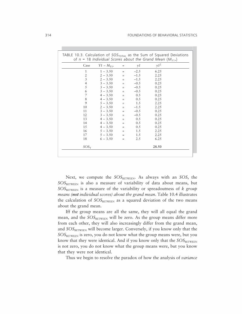
Next, we compute the SOSBETWEEN. As always with an SOS, theSOSBETWEEN is also a measure of variability of data about means, butSOSBETWEEN is a measure of the variability or spreadoutness of k groupmeans (not individual scores) about the grand mean. Table 10.4 illustratesthe calculation of SOSBETWEEN as a squared deviation of the two meansabout the grand mean.

Iff the group means are all the same, they will all equal the grandmean, and the SOSBETWEEN will be zero. As the group means differ morefrom each other, they will also increasingly differ from the grand mean,and SOSBETWEEN will become larger. Conversely, if you know only that theSOSBETWEEN is zero, you do not know what the group means were, but youknow that they were identical. And if you know only that the SOSBETWEEN

is not zero, you do not know what the group means were, but you knowthat they were not identical.

Thus we begin to resolve the paradox of how the analysis of variance


TABLE 10.3. Calculation of SOSTOTAL as the Sum of Squared Deviationsof n = 18 Individual Scores about the Grand Mean (MY1.)

Case Y1 – MY1. = y1 y12

1 1 – 3.50 = –2.5 6.252 2 – 3.50 = –1.5 2.253 2 – 3.50 = –1.5 2.254 3 – 3.50 = –0.5 0.255 3 – 3.50 = –0.5 0.256 3 – 3.50 = –0.5 0.257 4 – 3.50 = 0.5 0.258 4 – 3.50 = 0.5 0.259 5 – 3.50 = 1.5 2.25

10 2 – 3.50 = –1.5 2.2511 3 – 3.50 = –0.5 0.2512 3 – 3.50 = –0.5 0.2513 4 – 3.50 = 0.5 0.2514 4 – 3.50 = 0.5 0.2515 4 – 3.50 = 0.5 0.2516 5 – 3.50 = 1.5 2.2517 5 – 3.50 = 1.5 2.2518 6 – 3.50 = 2.5 6.25

SOSY 28.50

can test whether group dependent variable means are equal, given thatlocation and dispersion are two separate characterizations of data. Thedispersion of the Yi scores, measured in the SOSY, tells us nothing aboutwhat will be the numerical value for MY. But the SOSY and the SOSBETWEEN

are two different characters, and the SOSBETWEEN (unlike the SOSTOTAL)directly quantifies the magnitude of mean differences.

Finally, we compute the SOSWITHIN. We could do so by subtraction(i.e., SOSTOTAL – SOSBETWEEN), but then the meaning and relevance ofSOSWITHIN would be lost to us. SOSWITHIN is the sum of the k SOS valueswithin the various groups, calculated separately as squared deviations ofscores within each group about each group’s own individual kth groupmean, ignoring both all other groups and the grand mean, and thenpooled together.

We shall soon see that this pooling is reasonable iff certain circum-stances are met. And if the pooling used to compute the SOSWITHIN isunreasonable, then the ANOVA process and both its statistical and practi-cal significance results may be fatally compromised. Table 10.5 illustratesthese calculations for the heuristic data.

Conceptually, what is SOSWITHIN, and why is SOSWITHIN used inANOVA computations? In Chapter 3, we learned that all means do not doequally well at representing a set of scores. For example, for a given dataset, if SD is zero, the mean does a spectacular job of representing thescores. But if SD is huge, the mean serves poorly, and indeed may serve sopoorly at characterizing central tendency as to be nonsensical. Justbecause we can compute a statistic does not mean that the statistic isalways sensible!

The SOSWITHIN computes the outcome variable dispersion separately in


TABLE 10.4. SOSBETWEEN as the Weighted (by nk) Sum of SquaredDeviations of k = 2 Group Means about the Grand Mean (MY1.)

Group Mk – MY1. = y1k y1k2 × nk = SOSk

1 3.00 – 3.50 = –0.5 0.25 × 9 = 2.252 4.00 – 3.50 = 0.5 0.25 × 9 = 2.25

SOSBETWEEN 4.50

each group, and then pools these estimates. The separate estimates quan-tify how well each group mean does at representing the scores in a givengroup. The pooled estimate quantifies for the means as a set how wellthese means do at representing the scores in the respective groups.

Based on these considerations, would the mean differences on Y1 andY3 be equally noteworthy, given that the mean difference in both casesequals 1.0? Would the mean differences on Y2 and Y4 be equally note-worthy, given that the mean difference in both cases equals 2.0? Whichcombination of (a) means and (b) within-group dispersions least contra-dicts a null hypothesis assumption that the two means are equal? Whichcombination of (a) means and (b) within-group dispersions most contra-dicts a null hypothesis assumption that the two means are equal?


TABLE 10.5. SOSWITHIN as the Pooling of the SOS’sComputed Separately Within Each k Group,

Ignoring Both the Other Group and the Grand Mean

Case Y1 – Mk = y1 y12

1 1 – 3.00 = –2.0 4.002 2 – 3.00 = –1.0 1.003 2 – 3.00 = –1.0 1.004 3 – 3.00 = 0.0 0.005 3 – 3.00 = 0.0 0.006 3 – 3.00 = 0.0 0.007 4 – 3.00 = 1.0 1.008 4 – 3.00 = 1.0 1.009 5 – 3.00 = 2.0 4.00

Subtotal 12.00

10 2 – 4.00 = –2.0 4.0011 3 – 4.00 = –1.0 1.0012 3 – 4.00 = –1.0 1.0013 4 – 4.00 = 0.0 0.0014 4 – 4.00 = 0.0 0.0015 4 – 4.00 = 0.0 0.0016 5 – 4.00 = 1.0 1.0017 5 – 4.00 = 1.0 1.0018 6 – 4.00 = 2.0 4.00

Subtotal 12.00SOSWITHIN 24.00

�� Practical and Statistical Significance

The sums of squares partitions can be employed to estimate the effect sizeassociated with group differences, in a metric like that of r2. This estimateis called η2, or synonymously, the correlation ratio:

η2 = SOSBETWEEN / SOSTOTAL (10.3)

The correlation coefficient and the correlation ratio are two distinctconcepts, even though the first word of the their two-word names is thesame. The r is a score-world statistic, and η2 is an area-world statistic.

Note that Equation 10.3 is remarkably similar to Equations 8.5 and8.6, which are formulas for estimating the r2 and the R2 effect sizes! Thus,key elements of the general linear model are beginning to emerge.

Nevertheless, also recognize that r2 is a measure of linear relationshipbetween two intervally-scaled variables. The η2 quantifies how much ofthe variability in the Yi scores, measured as SOSY, we can explain or pre-dict with knowledge only about the group membership of each partici-pant. Thus, η2 involves one intervally-scaled variable, and one nominally-scaled variable, and not two intervally-scaled variables. And it makes nosense to talk about linear relationship in the context of one of two nomi-nally-scaled variables because the concept of linearity itself only makessense in a context, such as a scattergram, in which both axes are demar-cated by intervals for continuous variables.

So, η2 is a measure of relationship sensitive to all sorts of relationship,and not just linear relationship. For the Table 10.2 data, the η2 values are15.8% (i.e., 4.50 / 28.50), 42.8%, 36.0%, and 69.2%, respectively.

Just as the uncorrected effect size r2 / R2 can be “corrected” (e.g.,Ezechiel, 1930), the η2 can be adjusted to remove estimated capitalizationon sampling error. One such correction is Hays’ (1981) ω2.

The starting point in the calculation of ω2 requires the entries in thevariance partitions summary table, such as that presented for regression inTable 9.1. Given the general linear model, the basic computations are sim-ilar in ANOVA. One difference is that the sums of squares are computeddifferently, but once in hand, we manipulate these in parallel fashion. Andin regression the dfEXPLAINED equals the number of predictor variables,


whereas in one-way ANOVA, the dfBETWEEN is k – 1. Using the sums ofsquares computed in Tables 10.3, 10.4, and 10.5, Table 10.6 presents thesummary table for the tests of mean differences on Y1.

Hays’ ω2 can be computed as

ω2 = [SOSBETWEEN – (k – 1)MSWITHIN] / [SOSY + MSWITHIN] (10.4)

where k is the number of levels in the ANOVA way. For our data we have

[4.50 – (2 – 1)1.50] / [28.50 + 1.50][4.50 – (1)1.50] / [28.50 + 1.50]

[4.50 – (1)1.50] / 30.00[4.50 – 1.50] / 30.00

3.00 / 30.00ω2 = 10.0%

As explained in Chapter 7, and illustrated in Table 7.1, corrected effectsizes are equal to or smaller than their uncorrected counterparts. The dif-ference (i.e., “shrinkage”) is greater when (a) sample size is small, (b) thenumber of measured variables is larger, or (c) the population effect size issmaller. Here we had an n = 18 for our η2 = 15.8%, so shrinkage to ω2 =10.0% is not an undue surprise.

One can also use the sums of squares variance partitions to test thestatistical significance of the differences in the group means. When eitherthe levels of the way exhaust all possible values of the way (e.g., gender inhumans is measured at two levels), or the levels being used are the onlyones of interest to the researcher (e.g., we collect data only from freshmenand seniors, because we only care about freshmen and seniors for a given


TABLE 10.6. Variance Partitions for the MY1 Comparisons

Source SOS df MS FCALCULATED pCALCULATED η2 ω2

Between 4.50 1 4.50 3.00 0.102 15.8% 10.0%Within 24.00 16 1.50Total 28.50 17 1.68

Note. For ANOVA, the dfBETWEEN = the numbers of groups minus 1 (i.e., dfBETWEEN = k – 1).

purpose), the NHSST TS using the F distribution is calculated by dividingthe MSBETWEEN by the MSWITHIN. This FCALCULATED can be reexpressed aspCALCULATED by invoking the Excel spreadsheet function

=FDIST(FCALCULATED,dfBETWEEN,dfWITHIN)

�� The “Homogeneity of Variance” Assumption

As explained previously, the SOSWITHIN is computed by calculating sepa-rately the sums of the squared deviations from the group mean withineach group, ignoring both all other groups and the grand mean. Then thecell sums of squares are “pooled” by adding them together, yieldingSOSWITHIN. This pooling process is legitimate iff (if, and only if) thevariabilities of the scores in each group are roughly the same. This is theso-called homogeneity (equality) of variance assumption required inANOVA.

When we pool, we are invoking a kind of averaging process, or atleast a summation similar to that which we use in computing the numera-tor for the mean. It is not reasonable to lump things together when theyare wildly disparate.

This homogeneity of variance assumption is necessary both for statis-tical significance testing and for effect size interpretation. The conse-quences of meeting or not meeting this assumption can be concretelydemonstrated using some small hypothetical datasets.

Equal Group Means, Equal Group Variances

Figure 10.2 presents hypothetical data for a three-group one-way ANOVAwith five people in each cell. The five scores in each cell are exactly equally“spread out” (i.e., the homogeneity of variance assumption is exactly metin all three groups). The group means are also equal (i.e., all 3.0), and thegrand mean is 3.0, too. As noted earlier, because SOSBETWEEN is the sum ofthe squared deviations of the group means from the grand mean, when thegroup means are all the same, the SOSBETWEEN will be zero.

Figure 10.2 presents the computations confirming that the expected


outcome is realized. The SOSBETWEEN and the η2 equal zero when the groupmeans are equal. The figure uses different computational procedures thanthose illustrated in Tables 10.3, 10.4, and 10.5, but the procedures arealgebraically equivalent. Because we have perfectly met the homogeneityof variance assumption, at least as regards this assumption we can fullytrust both the ANOVA practical and NHSST results.


FIGURE 10.2. ANOVA example (n = 15, k = 3) with equal means, equal variances

Equal Group Means, Unequal Group Variances

Figure 10.3 presents hypothetical data for a three-group one-way ANOVAwith five people in each cell. Here the five scores in each cell vary in their“spreadoutness” (i.e., the scores in group 1 are the least spread out, andthe scores in group 3 are the most spread out). However, the group meansare all equal (i.e., all group means equal 3.0, and the grand mean is 3.0,too).


FIGURE 10.3. ANOVA example (n = 15, k = 3) with equal means, unequal variances

Even though the homogeneity of variance assumption is no longer metperfectly, because the three means are all identical, the effect size and sta-tistical significance results remain unchanged. Thus, if there are no groupmean differences, ANOVA results will not be distorted even if the homo-geneity of variance assumption is violated.

Unequal Group Means, Equal Group Variances

Figure 10.4 presents hypothetical data for a three-group one-way ANOVAwith five people in each cell. The five scores in each cell have exactly thesame amount of “spreadoutness.” However, the group means are now dif-ferent (i.e., 2.0, 3.0, and 4.0, respectively, while the grand mean is still3.0). Now the η2 effect size (SOSBETWEEN / SOSTOTAL) is 25%, andFCALCULATED is 2.00. The results honor the differences in the means, andbecause the homogeneity of variance assumption is met perfectly, we canvest confidence in a conclusion that the result is not an artifact of violatinga statistical assumption.

Unequal Group Means, Unequal Group Variances

Figure 10.5 presents hypothetical data for a three-level one-way ANOVAwith five people in each cell. The five scores in each cell no longer haveexactly the same amount of spreadoutness. However, the group means arestill different (i.e., 2.0, 3.0, and 4.0, respectively, while the grand mean isstill 3.0). Now the effect size (SOSBETWEEN / SOSTOTAL) is 20%, andFCALCULATED is 1.50.

Even though the magnitude of the mean differences is identical tothose in the previous example, both effect size and statistical significanceresults in this example have been attenuated, because the homogeneity ofvariance assumption has been violated to some degree. It is important tonote that such violations can lead to degrees of distortion causing theunwary researcher to make entirely unjustified interpretations.

Testing Homogeneity of Variance Using NHSST

The homogeneity assumption requires an assertion that the populationvariances of the dependent variable scores for each group are the same


(e.g., SD12 = SD2

2 = SD32). This, of course, is the null hypotheses that the

dependent variable score variances are equal across the groups. Someresearchers elect to evaluate the homogeneity of variance assumption byusing the statistical significance tests available within software ANOVAprocedures. For the two-group situation, for either the two-sample t testor one-way, two-level ANOVA, NHSST results may be obtained by invok-


FIGURE 10.4. ANOVA example (n = 15, k = 3) with unequal means, equal variances

ing Equation 6.3. For three or more groups, a test proposed by Levene(1960) may be used.

Using NHSST to evaluate whether methodological assumptions aremet (and thus the researcher hopes that the test of this H0 is not statisti-cally significant) can suggest a paradox. As Thompson (1994c) noted,

The researcher desirous of statistically significant effects for substantive main


FIGURE 10.5. ANOVA example (n = 15, k = 3) with unequal means, unequal variances

and interaction effects will quite reasonably employ the largest sample possi-ble so as to achieve the hoped-for results. Regrettably, large samples that tendto yield significance for substantive tests also tend to yield statistically signifi-cant results leading to rejection of method assumption null hypotheses, as inthe test of equality of dependent variable variances across groups required bythe ANOVA homogeneity of variance assumption. (p. 13)

The implication is that common sense (and effect sizes), and not justNHSST, must be used to evaluate whether the homogeneity of varianceassumption has been reasonably well met.

Unfortunately, empirical studies of published research show thatresearchers too often ignore the assumptions of their statistical methods(Keselman et al., 1998). These assumptions are more important than manyresearchers realize, as suggested by Wilcox (1998) in his article titled“How many discoveries have been lost by ignoring modern statisticalmethods?”

�� Post Hoc Tests

If the omnibus null hypothesis is not rejected, the researcher’s analytictasks are completed. On the other hand, iff both (a) the omnibus null isrejected, and (b) the way has more than two levels, further analyses arerequired to determine which group means differ. Perhaps every mean dif-fers to a statistically significant degree from every other mean. Or, at theother extreme, perhaps only one mean differs from all the other means,none of which, in turn, differ from each other.

Some have argued that some post hoc tests may be invoked in thepresence of three or more groups, even if the omnibus hypothesis is nottested or rejected. However, what are described here are the most commonpractices as of this date.

Post hoc tests are analyses conducted following the rejection of anomnibus null involving three or more levels to investigate more specificallywhich group means differ. There are many names for these analyses, someof which are summarized in Table 10.7. The alternative names are con-structed by selecting one entry from the first column of the table and pair-


ing the selection with one entry chosen from the second column of thetable (e.g., post hoc contract, a posteriori comparison).

Post hoc analysis can be conceptualized in converse, but equallyappropriate, terms as detecting how many homogeneous subsets there arewithin the means. For example, given a six-level way, if one mean differedfrom the remaining five, none of which differed to a statistically significantdegree from each other, there would be two homogeneous subsets. Or, ifall six means differed to a statistically significant degree each from everyother, there would be six homogeneous subsets of means.

Or, among the ordered means, the first two means might not differfrom each other, but the first mean might differ from means three throughsix, and the second mean might not differ from the third mean, but mightdiffer to a statistically significant degree from means four through six, andso forth. Figure 10.6 presents a graphic representation of such an analysis,yielding five homogeneous subsets among the six means.

One among several alternative reporting formats uses superscripts.For example, the researcher may report the results of these analyses by


TABLE 10.7. Synonymous Namesfor ANOVA Post Hoc Tests

Phrase elements

First Second

post hoc contrasta posteriori comparisonunfocused testunplannedfollow-up

FIGURE 10.6. Graphic representation of results from a post hoc analysis

saying, “The group means were M1 = 10.5a, M2 = 15.2a,b, M3 = 19.8b,c,M4 = 24.9c,d, M5 = 30.2d,e, and M6 = 35.1e,” where means with commonsuperscripts do not differ to a statistically significant degree.

Researchers using ANOVA soon realized the importance of conduct-ing post hoc analyses for statistically significant omnibus hypothesesinvolving three or more levels. Of course, if a way has exactly two levels(e.g., boys versus girls), post hoc methods are unnecessary even if theomnibus null is rejected, because we know exactly where such differencesarise (i.e., boys and girls must differ, “duh”—or if you are Australian,“der”).

Post hoc contrasts compare two means. Simple contrasts compare theoutcome variable mean of one level of the way with the outcome variablemean of another level of the way (e.g., H0: MFRESHMEN = MSOPHOMORES, or“the dependent variable mean of the 10 freshmen equals the dependentvariable mean of the 10 sophomores”). No levels are combined to createeither (or both) of the two means being compared using simple contrasts.Complex contrasts compare two means, either one or both of which arecomputed by creating means from combining levels of the way (e.g., H0:MFRESHMEN = MSOPHOMORES, JUNIORS; H0: MFRESHMEN = MSOPHOMORES, JUNIORS, SENIORS;H0: MFRESHMEN, SOPHOMORES = MJUNIORS, SENIORS, or “the dependent variablemean of the 20 students who are either freshmen or sophomores equalsthe dependent variable mean of the 20 students who are either juniors orseniors”).

At first pale the use of conventional t tests to conduct post hoc analy-ses might have some appeal, because post hoc tests evaluate whether twomeans are equal, and two-sample t tests can be used to evaluate the equal-ity of two means. But one reason we are using ANOVA in the first place isto avoid the inflation of the experimentwise error rate. Of course, an argu-ment might be made that the experimentwise error rate would be inflatedless severely if we only conducted t tests following the rejection of anomnibus null, rather than using t tests straightaway and without testingthe omnibus. Indeed, this “protected” t testing would be less problematicthan the unprotected counterpart.

However, there are serious difficulties with using conventional t testsfor post hoc analyses. For example, even using protected t tests post hocwhen evaluating means results in some experimentwise error rate infla-tion. Also, we would not be taking into account how many means are


being compared. For example, the error rate inflation from using pro-tected t tests would not be equal in one study involving 3 levels versusanother study involving 10 levels.

In addition, using conventional t tests would not take into account thenumber of contrasts we are conducting, even across situations involvingthe same number of means. For example, given a three-level way, accord-ing to Equation 6.2 ([3 (3 – 1)] / 2), three simple contrasts are possible.Three complex contrasts are also possible: {1 vs. 2,3}, {2 vs. 1,3}, and{3 vs. 1,2}. Thus, for a three-level way, there are three post hoc tests if onlysimple contrasts are being conducted, but there are six post hoc tests ifboth simple and complex contrasts are being conducted.

If we have a four-level way, there are six possible simple contrasts([4(4 – 1)] / 2). But there are 19 complex contrasts for this design:

{1 vs. 2,3} {1 vs. 2,4} {1 vs. 3,4}{2 vs. 1,3} {2 vs. 1,4} {2 vs. 3,4}{3 vs. 1,2} {3 vs. 1,4} {3 vs. 2,4}{4 vs. 1,2} {4 vs. 1,3} {4 vs. 2,3}{1,2 vs. 3,4} {1,3 vs. 2,4} {1,4 vs. 2,3}{1 vs. 2,3,4} {2 vs. 1,3,4} {3 vs. 1,2,4} {4 vs. 1,2,3}

Clearly, as we have more levels, (a) the number of possible contrastsexpands quite rapidly, and (b) the discrepancy between the number of onlysimple contrasts versus the number of both simple and complex contrastsexpands as well.

Beginning in the 1950s, statisticians began to propose dozens of modi-fied t test procedures that take into account (a) how many group means orlevels and (b) how many contrasts (i.e., only simple, or both simple andcomplex) are being considered. Conceptually, these post hoc methods canbe thought of as being special t tests that invoke a Bonferroni-type correc-tion taking into account the number of post hoc hypothesis tests. Actually,the methods adjust the critical value of the test statistic to take these issuesinto consideration.

Commonly used post hoc tests do either (a) only simple or (b) bothsimple and complex contrasts, and they do all the contrasts available for agiven situation. Thus, for a three-level way, a post hoc method that evalu-


ates only simple contrasts tests all three of the possible simple contrasts,and a post hoc method that does both simple and complex contrasts doesall six of the possible contrasts.

An important implication of this is that (a) post hoc tests might evalu-ate contrasts not of interest to you and (b) force you to pay for testinguninteresting hypotheses as part of the Bonferroni-type correction. As weshall see in Chapter 12, we can escape this potentially unsavory situationby using planned contrasts instead.

Two of the most commonly used of the myriad post hoc tests are theTukey and the Scheffé tests. Tukey post hoc tests evaluate all (and only)the simple contrasts available for a given design. Thus, the correction con-siders only simple contrasts, but will nevertheless differ for designs withk = 3, versus k = 4, versus k = 5 levels. Scheffé post hoc tests evaluate allthe both simple and complex contrasts that are available for a givendesign. Thus, the Scheffé corrections for a k = 3 design are more severethan are the Tukey corrections for a k = 3 design. And the gaps betweenthe amounts of correction between Tukey and Scheffé methods grow rap-idly as more levels are involved in the design. One consequence of theseadjustment dynamics is that Scheffé tests have considerably less powerthan Tukey tests, especially as the number of levels increases.

Clearly, if only simple contrasts are of interest, of the two choices dis-cussed here Tukey tests are the correct choice. If complex contrasts are ofinterest, especially when the ways have many levels, Scheffé methods willbe more appealing when the sample size is very large, so that power willremain reasonable even with these tests. Note that with some post hoctests, including choices not considered here, it is possible to reject the nullomnibus hypothesis and then find none of the post hoc tests statisticallysignificant.

Some Key Concepts

For a two-level one-way design, the two-sample t test and one-wayANOVA of the same data yield identical pCALCULATED and effect sizestatistics. For one-way designs involving more than two levels, the useof all possible pairwise two-sample t tests will result in inflatedexperimentwise error rates. To avoid this problem, and for other rea-sons explained in Chapter 11, ANOVA is used only to test mean dif-


ferences for three or more groups, and can be used to test meandifferences involving only two groups. ANOVA can be used to testonly the statistical significance of mean differences, or only the practi-cal significance of these differences, or both.

ANOVA requires an assumption that in the population the dis-persions of the dependent variable scores are equal across the groups.The failure to meet this homogeneity of variance assumption maycompromise the accuracy of both NHSST and effect size statistics.

When an omnibus null hypothesis is rejected and the way hasthree or more levels, post hoc tests are necessary to determine wherethe mean differences lie. Post hoc tests evaluate either simple (e.g.,Tukey tests) or both simple and complex contrasts (e.g., Scheffé tests).Because for a given design Scheffé tests evaluate more hypotheses, andtherefore invoke a stronger Bonferroni-type correction, Scheffé testshave less power against Type II error.


1. Consider the outcome variable scores for three studies involving balanced

one-way two-level ANOVAs.

Study A

Group 1: 8, 9, 10; M = 9; Group 2: 10, 11, 12; M = 11

Study B

Group 1: 7, 8, 9; M = 8; Group 2: 11, 12, 13; M = 12

Study C

Group 1: 7, 9, 11; M = 9; Group 2: 9, 11, 13; M = 11

Effect sizes are zero when sample statistics exactly match the expecta-

tions specified in the null hypothesis. For each of the three studies, what

is the effect size for the homogeneity of variance hypothesis? Is the effect

size zero for the null hypothesis tested by ANOVA in any of the three

studies?

In Study A versus Study B, which, if any, of the three sums of squares

(i.e., total, between, within) will be equal? In Study A versus Study C,

which, if any, of the three sums of squares (i.e., total, between, within)


will be equal? The mean difference (M1 = 9; M2 = 11) is the same for

Study A and Study C, the homogeneity of variance assumption is per-

fectly met in both studies, and the ns are the same across the two stud-

ies. Will the pCALCULATED be equal for these two studies?

What is the rank ordering of the pCALCULATED values for the three stud-

ies? Are the three η2 values equal across any of the studies?

2. Run omnibus ANOVA tests for each of the four outcome variables pre-

sented in Table 10.2. Compare and contrast the ANOVA results for (1) Y1

versus Y2, (2) Y1 versus Y3, (3) Y4 versus Y2, and (4) Y4 versus Y3. What

explains the dynamics reflected in these comparisons? What two issues

drive ANOVA tests? Why is it (perfectly) reasonable that both these fac-

tors drive ANOVA results?

3. Limiting the discussion to n = 8, and with possible scores of only {1, 2, 3,

4, 5}, what 8 scores would yield the mathematically maximum values of

dispersion for this context? What are the mathematically maximum

values of (a) the sum of squares, (b) the variance, and (c) the SD, for this

context? Draw the histogram of these data.

Next, let’s now assume that the data involve a two-level one-way

ANOVA problem, with two groups of scores. We have already computed

the SOSTOTAL. Compute (a) the SOSBETWEEN and (b) the SOSWITHIN. Why

does the SOSWITHIN yield this result for these data?

In Chapter 3, I emphasized that every report of a mean should include

a report of the related SD, and that the SD quantifies how well a given

mean does at representing all the scores. In ANOVA, the SOSBETWEEN

quantifies the degree of mean differences. What will SOSBETWEEN be for a

two-level one-way ANOVA if the two dependent variable means are

equal? What will SOSBETWEEN be for a four-level one-way ANOVA if the

four dependent variable means are equal?

In descriptive statistics, the SD for the dataset quantifies how well the

group mean does at representing all the scores in the dataset. In ANOVA,

does the SOSWITHIN perform an analogous function of quantifying how

noteworthy the groups’ mean differences are, by taking into account as

part of the mean comparison how well each mean does at representing

the scores in each group?


4. The effect sizes for a given design are context-driven. For example, if we

explore the effects on myocardial infarcts of being randomly assigned to

take 81, 325, or 750 milligrams of aspirin daily, we cannot conclusively

extrapolate findings to cover taking 2,500 milligrams of aspirin daily. So,

too, if studies cover similar but different dosages, the effect sizes cannot

be directly compared exactly apples-to-apples. But can the effects be

rescaled to take design differences into account? Consult Fowler (1987),

Olejnik and Algina (2003), and Ronis (1981) to help clarify your views.


11

Multiway andOther Alternative

ANOVA Models

In Chapter 10, only one-way designs were considered. In this chapter,multiway designs are introduced. The use of nonfactorial models isdiscussed. And the possibilities of fixed-, random-, and mixed-effectsmodels are considered.

�� Multiway Models

One-way ANOVA for k greater than two levels represented an importantadvance over the alternative of conducting all possible pairwise t tests,thus avoiding the associated experimentwise Type I error rate inflation.However, multiway ANOVA designs afford two additional advantagesover alternative analyses.

First, design efficiencies can be realized by evaluating two or moreomnibus hypotheses within a single study rather than across separate stud-ies. For example, if we wish to evaluate the effects of three dosages of drug

333

A on blood pressure and four alternative dosages of drug B on blood pres-sure, we can conduct a single two-way 3 × 4 ANOVA, rather than two in-dependent one-way ANOVAs. We will theoretically obtain equivalentresults across these alternatives, if sample sizes are compared apples-to-apples. So, we can answer more questions in fewer studies by usingmultiway ANOVA.

Second, and perhaps more importantly, as noted in Chapter 9,researchers are often keenly interested in testing interaction effects, andmultiway ANOVA can be used to investigate these effects, just as interac-tion effects can be tested in regression. Investigating which educational ortherapy intervention works best for everybody may be interesting, but alsomay be quixotic. Investigating in the same study which treatment worksbest for whom is important, and usually essential. In reality, few treat-ments work best (or worst) for every conceivable group of people(Cronbach, 1957).

Terminology

A main effect is an omnibus effect that evaluates differences in dependentvariable means across all the levels of a given way, ignoring all the levels ofall the remaining ways. An interaction effect evaluates the joint impacts ofthe combinations of the levels from two or more ways on the differences inthe dependent variable means, ignoring all the levels of all the ways notinvolved in the interaction.

For example, in the previously described 3 × 4 design, if the designwas balanced with 10 people in each cell, the total sample size would be120. Two main effect null hypotheses may be tested:

(a) The mean blood pressure of the 40 people taking dose 1 of drug Aequals the mean blood pressure of the 40 people taking dose 2 ofdrug A equals the mean blood pressure of the 40 people takingdose 3 of drug A, and

(b) the mean blood pressure of the 30 people taking dose 1 of drug Bequals the mean blood pressure of the 30 people taking dose 2 ofdrug B equals the mean blood pressure of the 30 people takingdose 3 of drug B equals the mean blood pressure of the 30 peopletaking dose 4 of drug B.


Note that ANOVA, unlike the conventional t test, which cannot eval-uate interaction effects, readily handles tests of interaction hypotheses. Forthis design, only one interaction hypothesis, the two-way A × B interactioneffect, may be tested. However, designs with more levels accommodatemore main and interaction effect tests. For example, all three-way designscan involve testing three main effects, three two-way interaction effects,and one three-way interaction effect. A four-way design can involve test-ing four main effects, six two-way interaction effects, four three-way inter-action effects, and one four-way interaction effect.

Mathematically, it can be proven that for any balanced design, allpairs of all main and interaction hypotheses are perfectly uncorrelated (seeHester, 2000, pp. 22–27). Consequently, the sums of squares for all effectsin a balanced design are unique for a given effect and, together with theSOSERROR, sum to equal the SOSY exactly.

This property, that omnibus hypotheses are perfectly uncorrelated forall balanced ANOVA designs, was noteworthy for two reasons. First, abalanced ANOVA can be effectively thought of as a Case #1 regressionsituation. And, as we saw in Chapter 9, all the computations necessary foran analysis in this situation are vastly simplified. The computational sim-plicity accomplished through the magic of the ANOVA logic, which yieldsperfectly uncorrelated, nonoverlapping effects for balanced designs, washugely important in the decades when all computations had to be per-formed (repeatedly, to check for calculation errors) on calculators.

Second, obtaining nonoverlapping or unique effects for each omnibustest also hugely simplifies result interpretation, just as regression resultinterpretation is simplified in Case #1. If 10% of the SOSY is predicted orexplained by information about to which levels of way A the participantsbelonged, and if that 10% has no commonality with any other effect,there is no debate about allocating nonexistent common predictive credit.

Computational Example

We will reuse the Table 9.3 blood alcohol data to illustrate the computa-tions for a factorial 2 × 2 analysis. Here, again, we are partitioning theinformation regarding the amount and origins of individual differencesquantified by the SOSTOTAL of 0.124. The small number even for n = 32

11. Multiway and Other Alternative ANOVA Models 335

participants suggests that blood alcohol levels do not vary much, on aver-age, even when people have had up to seven drinks. Of course, on thisvariable, small score differences can yield huge differences in motor skills,such as those required to operate an automobile. Clearly, what makes agiven SOS large or small depends on what variable we are measuring.

For the purposes of this analysis, because ANOVA requires nomi-nally-scaled data on the independent variables, we have mutilated theintervally-scaled scores on the two predictors to yield dichotomies. Youshould find this troubling. When, if ever, would one be willing to muti-late interval independent variables simply so that ANOVA could beused?

However, the mutilation does afford us the heuristic opportunity tocompare apples-to-apples effects for the nonmutilated and the mutilateddata. And remember that this comparison is made within the context of asingle study.

When such mutilations are made across the studies in a literature, theconsequences may be quite dire. If all researchers mutilated their intervalpredictors by using sample-specific medians, the medians may well differin each sample, and then, when the ANOVA results are inconsistent acrossstudies, we do not know whether (a) the inconsistencies across studiesoccurred because results were unstable across samples, or (b) the varia-tions in median cutpoints used to create groups made consistency unat-tainable, and the findings irreconcilable.

More will be said later on the question of mutilation of intervally-scaled data. Table 11.1 presents the Table 9.3 data after the intervally-scaled predictors have been converted into nominal scale.

First, we will compute the two main effect sums of squares. We coulduse the same procedures described in detail in Chapter 10, but will insteaduse algebraically-equivalent formulas that yield identical results. Theseformulas involve the outcome scores squared, and then summed (i.e., notthe SOS, because SOS is instead the sum of the squared deviations fromthe mean). Here, as reported in Table 11.1, the outcome scores squaredand then summed equal 0.4204. The formulas also require the sums of thescores in the four cells: Σ1,1, Σ1,2, Σ2,1, and Σ2,2. Last, the formulas requirethe sum of all the outcome scores, which is 3.08, as reported in Table11.1.



TABLE 11.1. Conversion of Table 9.13 Data into ANOVA Form

SPSS Variables

Group/case W_GRP DR_GRP BLOOD Cell total BLOOD2

Low weight, low drinks1 1 1 0.04 0.00162 1 1 0.11 0.01215 1 1 0.03 0.00096 1 1 0.09 0.00819 1 1 0.03 0.0009

10 1 1 0.08 0.006413 1 1 0.02 0.000414 1 1 0.07 0.47 0.0049

Low weight, high drinks3 1 2 0.19 0.03614 1 2 0.26 0.06767 1 2 0.16 0.02568 1 2 0.22 0.0484

11 1 2 0.13 0.016912 1 2 0.19 0.036115 1 2 0.12 0.014416 1 2 0.16 1.43 0.0256

High weight, low drinks17 2 1 0.02 0.000418 2 1 0.06 0.003621 2 1 0.02 0.000422 2 1 0.06 0.003625 2 1 0.02 0.000426 2 1 0.05 0.002529 2 1 0.02 0.000430 2 1 0.05 0.30 0.0025

High weight, high drinks19 2 2 0.11 0.012120 2 2 0.15 0.022523 2 2 0.09 0.008124 2 2 0.13 0.016927 2 2 0.09 0.008128 2 2 0.12 0.014431 2 2 0.08 0.006432 2 2 0.11 0.88 0.0121

Sum 3.08 3.08 0.4204

The SOSWEIGHT, or the main effect SOS for weight, is computed as

SOSA = {[(Σ1,1 + Σ1,2)2 + (Σ2,1 + Σ2,2)2] / [j(n)]} – {Σ2 / [i(j)(n)]} (11.1)

where i is the number of levels in the A way, j is the number of levels in theB way, and n is the number of participants in each cell. For our data wehave

{[(0.47 + 1.43)2 + (0.30 + 0.88)2] / [2(8)]} – {3.082 / [2(2)(8)]}{[1.902 + 1.182] / [2(8)]} – {3.082 / [2(2)(8)]}

{[3.6100 + 1.3924] / [2(8)]} – {9.4864 / [2(2)(8)]}{5.0024 / [2(8)]} – {9.4864 / [2(2)(8)]}

{5.0024 / 16} – {9.4864 / 32}0.3127 – 0.2965

SOSWEIGHT = 0.0162

The SOSDRINKS, or the main effect SOS for drinks, is computed as

SOSB = {[(Σ1,1 + Σ2,1)2 + (Σ1,2 + Σ2,2)2] / [i(n)]} – {Σ2 / [i(j)(n)]} (11.2)


{[(0.47 + 0.30)2 + (1.43 + 0.88)2] / [2(8)]} – {3.082 / [2(2)(8)]}{[0.772 + 2.312] / [2(8)]} – {3.082 / [2(2)(8)]}

{[0.5929 + 5.3361] / [2(8)]} – {9.4864 / [2(2)(8)]}{5.9290 / [2(8)]} – {9.4864 / [2(2)(8)]}

{5.9290 / 16} – {9.4864 / 32}0.3706 – 0.2965

SOSDRINKS = 0.0741

The SOSWEIGHT × DRINKS is computed as

SOSA × B = {[Σ1,12 + Σ2,1

2 + Σ1,22 + Σ2,2

2] / n} (11.3)– SOSA – SOSB – {Σ2 / [i(j)(n)]}



{[0.472 + 1.432 + 0.302 + 0.882] / 8} – 0.0162 – 0.0741 – {3.082 / [2(2)(8)]}{[0.2209 + 2.0449 + 0.0900 + 0.7744] / 8}

– 0.0162 – 0.0741 – {9.4864 / [2(2)(8)]}{3.1302 / 8} – 0.0162 – 0.0741 – {9.4864 / [2(2)(8)]}

{3.1302 / 8} – 0.0162 – 0.0741 – {9.4864 / 32}0.3913 – 0.0162 – 0.0741 – 0.2965

SOSA × B = 0.0045

Notice that we subtract out of SOSA × B the main effect SOS thatreflects the differences of the two outcome variable means on both the Away and the B way. This reflects the reality that the differences in the fourcell means are jointly influenced by the interaction effect and both maineffects. One implication, as we will see momentarily, is that plotting thecell means to understand interaction effects can be misleading because, asthe title of Rosnow and Rosenthal’s (1991) article implies, “If you’re look-ing at the cell means, you’re not looking at only the interaction (unless allmain effects are zero).”

The SOSWITHIN is computed as

SOSWITHIN = Σ(Yi2) – {[Σ1,1

2 + Σ2,12 + Σ1,2

2 + Σ2,22] / n} (11.4)


0.4204 – {[0.472 + 1.432 + 0.302 + 0.882] / 8}0.4204 – {[0.2209 + 2.0449 + 0.0900 + 0.7744] / 8}

0.4204 – {3.1302 / 8}0.4204 – 0.3913

SOSWITHIN = 0.0291

These values can then be arrayed into the summary table reported in Table11.2.

The degrees of freedom for main effects equal the number of levels ina given way minus 1. This reflects the computation of SOSBETWEEN asinvolving all group means in the presence of the estimated grand mean(i.e., MY.). Given MY, only k – 1 of the group means are free to vary.


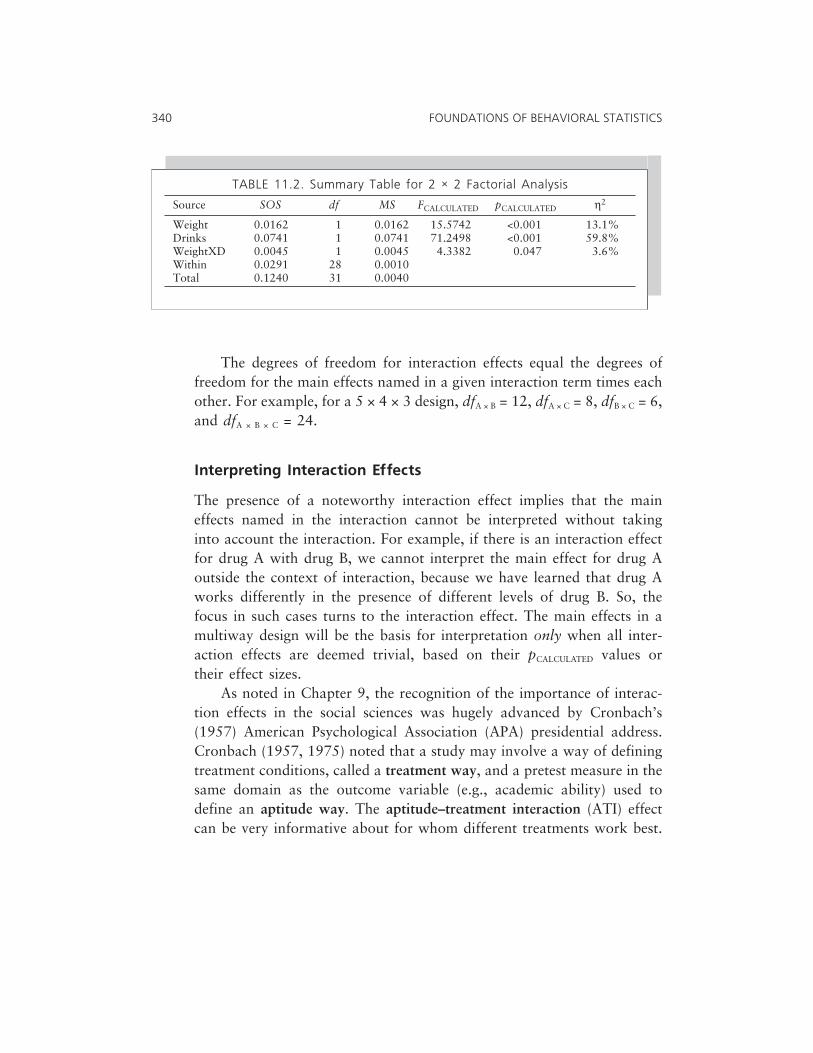
The degrees of freedom for interaction effects equal the degrees offreedom for the main effects named in a given interaction term times eachother. For example, for a 5 × 4 × 3 design, dfA × B = 12, dfA × C = 8, dfB × C = 6,and dfA × B × C = 24.

Interpreting Interaction Effects

The presence of a noteworthy interaction effect implies that the maineffects named in the interaction cannot be interpreted without takinginto account the interaction. For example, if there is an interaction effectfor drug A with drug B, we cannot interpret the main effect for drug Aoutside the context of interaction, because we have learned that drug Aworks differently in the presence of different levels of drug B. So, thefocus in such cases turns to the interaction effect. The main effects in amultiway design will be the basis for interpretation only when all inter-action effects are deemed trivial, based on their pCALCULATED values ortheir effect sizes.

As noted in Chapter 9, the recognition of the importance of interac-tion effects in the social sciences was hugely advanced by Cronbach’s(1957) American Psychological Association (APA) presidential address.Cronbach (1957, 1975) noted that a study may involve a way of definingtreatment conditions, called a treatment way, and a pretest measure in thesame domain as the outcome variable (e.g., academic ability) used todefine an aptitude way. The aptitude–treatment interaction (ATI) effectcan be very informative about for whom different treatments work best.


TABLE 11.2. Summary Table for 2 × 2 Factorial Analysis

Source SOS df MS FCALCULATED pCALCULATED η2

Weight 0.0162 1 0.0162 15.5742 <0.001 13.1%Drinks 0.0741 1 0.0741 71.2498 <0.001 59.8%WeightXD 0.0045 1 0.0045 4.3382 0.047 3.6%Within 0.0291 28 0.0010Total 0.1240 31 0.0040

The ATI designs are useful, because the search for the elusive treatmentthat is best for everyone may be unrealistic.

Unfortunately, the interpretation of interaction effects is not asstraightforward as the procedures recommended in many statistics text-books. Researchers have defined a Type IV error as occurring when anhypothesis is correctly rejected but the basis for the rejection is incorrectlyinterpreted (Levin & Marascuilo, 1972; Marascuilo & Levin, 1970). In arelated vein, Rosnow and Rosenthal (1989b) noted that interaction effectsare “probably the universally most misinterpreted empirical results in psy-chology” (p. 1282).

Many textbooks recommend the plotting of cell means to exploreinteraction effects, especially for two-way interaction effects. The verticalaxis is used (as always) to represent the outcome variable. Usually the hor-izontal axis is demarcated by the levels of the aptitude way (e.g., low,medium, and high IQ). Then symbols (e.g., circles and triangles) are usedto represent cell means across the treatment conditions (e.g., lecture versusdiscovery instruction, “talk” therapy versus behavior modification ther-apy). Like symbols are then linked by like continua (e.g., the three meansfor lecture are linked by a continuous line, while the three means for dis-covery methods are linked by a dashed line).

If a given treatment has higher means across the three IQ levels, thenarguably that treatment is best for all IQ groups, or at least the groups repre-sented within the study. If the plotted lines cross, then one treatment may bebest for some people, but the other treatments may be best for other people.

These ATI (or other interaction) plots do reflect real differences in thecell means. This information can be quite important from a practical pointof view. However, plots of the cell means do not reflect only interactioneffect dynamics.

Instead, the cell means used in these plots are impacted by the con-founded joint influences of a variety of factors. As noted by Rosnow andRosenthal (1989a), the cell means “are the combined effects of the interac-tion, the row effects [a main effect], the column effects [a second maineffect], and the grand mean” (p. 144). By the same token, simple post hoctests of the cell means also do not yield insight about the origins of interac-tion effects, because the interaction effects are not uniquely a function ofthe cell means (Boik, 1979).

Figure 11.1 presents the cell means, the margin means, and the grand


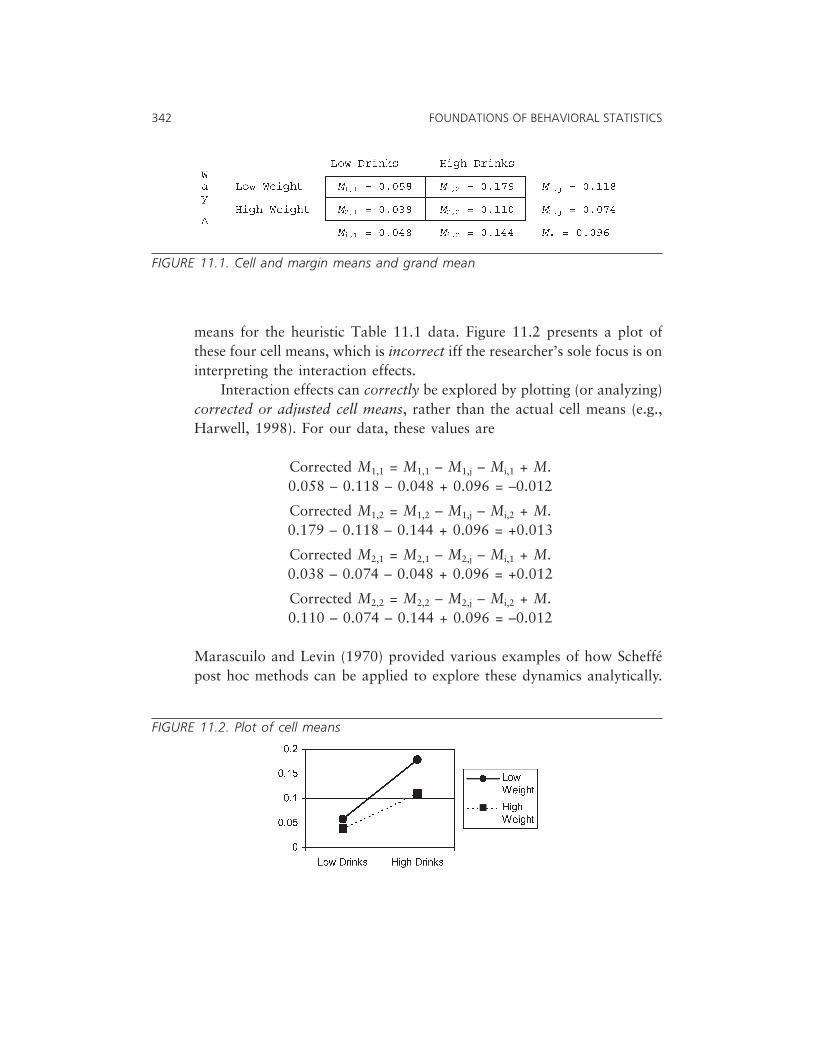
means for the heuristic Table 11.1 data. Figure 11.2 presents a plot ofthese four cell means, which is incorrect iff the researcher’s sole focus is oninterpreting the interaction effects.

Interaction effects can correctly be explored by plotting (or analyzing)corrected or adjusted cell means, rather than the actual cell means (e.g.,Harwell, 1998). For our data, these values are

Corrected M1,1 = M1,1 – M1,j – Mi,1 + M.0.058 – 0.118 – 0.048 + 0.096 = –0.012

Corrected M1,2 = M1,2 – M1,j – Mi,2 + M.0.179 – 0.118 – 0.144 + 0.096 = +0.013

Corrected M2,1 = M2,1 – M2,j – Mi,1 + M.0.038 – 0.074 – 0.048 + 0.096 = +0.012

Corrected M2,2 = M2,2 – M2,j – Mi,2 + M.0.110 – 0.074 – 0.144 + 0.096 = –0.012

Marascuilo and Levin (1970) provided various examples of how Scheffépost hoc methods can be applied to explore these dynamics analytically.


FIGURE 11.1. Cell and margin means and grand mean

FIGURE 11.2. Plot of cell means

The take-home message is not that plots of cell means are unimportantfrom a practical point of view, but instead is that such plots involve morethan interaction dynamics, and plots of adjusted means are of interest ifthe focus is on understanding interaction effects.

�� Factorial versus Nonfactorial Analyses

Factorial analyses test all possible main and interaction effects.Nonfactorial designs test at least one effect but fewer than all the possiblemain and interaction effects. One-way designs are inherently factorial. Forour illustrative 3 × 4 design, if we test all three possible omnibus hypothe-ses, the design is factorial. If we do not conduct any one or more of thepossible omnibus tests, the analysis is no longer factorial.

At first impression one might think that conducting a nonfactorialanalysis is illogical. If the ways are thoughtfully selected, does this notimply interest in all possible main and interaction effects? However, thereare two possible situations in which nonfactorial designs have appeal,although the decision in favor of a nonfactorial over a factorial design ofcourse turns upon thoughtful personal judgment of what is best in a givensituation.

First, in multiway designs with many ways, researchers might reason-ably forgo the testing of very high-order interaction effects. Even second-order effects can be complicated to interpret. Think of a five-way design inwhich the interpretation of the five-way interaction effect would requireconsideration of all the possible combinations of all levels conditionedupon each other in their effects on the outcome variable. Furthermore, themeans at the highest order involve the fewest participants per estimate,and so these effects theoretically are least stable.

Second, some researchers forgo testing main effects for ways that arenot malleable. For example, a researcher might conduct a 3 × 2 studyinvolving a treatment way with three levels, and a gender way. If we findas a main effect that women learn more than men, how can we apply ourknowledge? Many men will resist having their gender altered in service ofimproved outcome variable scores, no matter how persuasive an argumentis presented!


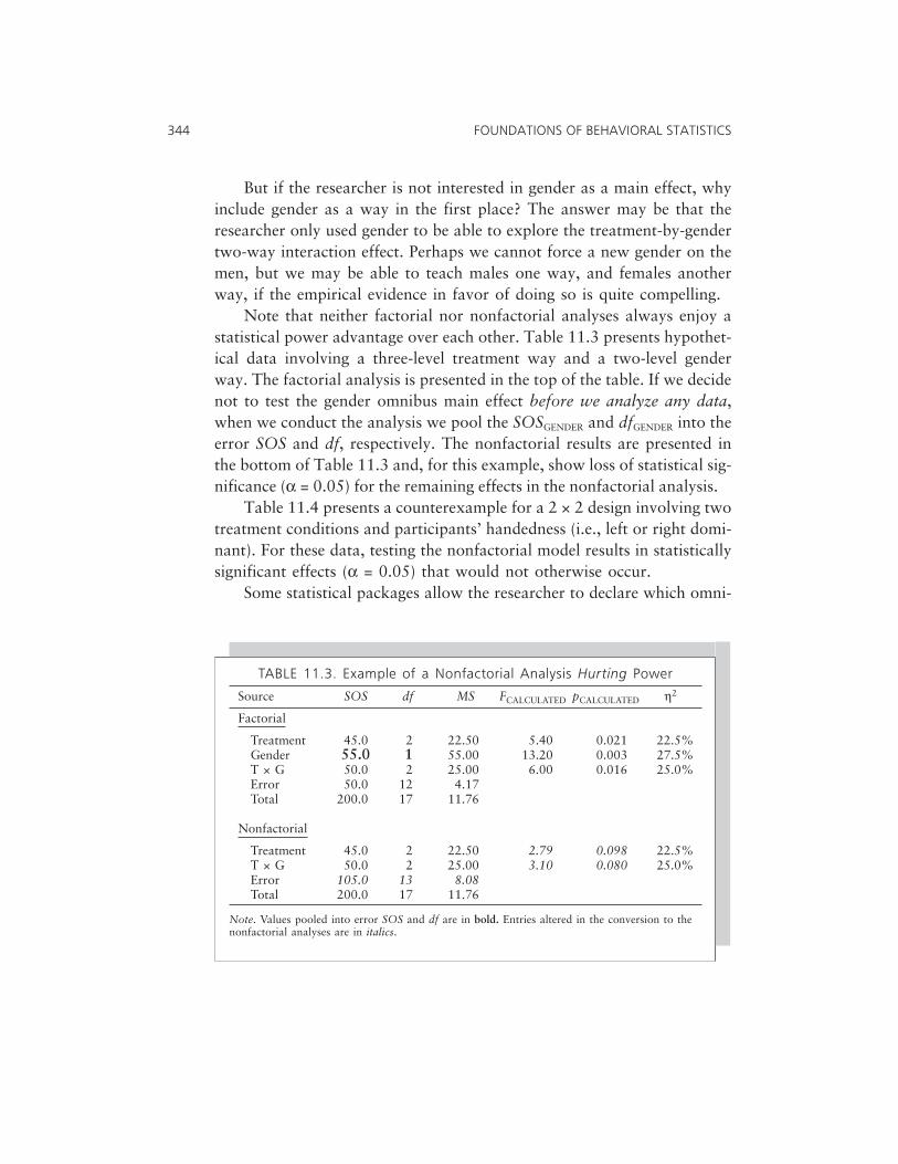
But if the researcher is not interested in gender as a main effect, whyinclude gender as a way in the first place? The answer may be that theresearcher only used gender to be able to explore the treatment-by-gendertwo-way interaction effect. Perhaps we cannot force a new gender on themen, but we may be able to teach males one way, and females anotherway, if the empirical evidence in favor of doing so is quite compelling.

Note that neither factorial nor nonfactorial analyses always enjoy astatistical power advantage over each other. Table 11.3 presents hypothet-ical data involving a three-level treatment way and a two-level genderway. The factorial analysis is presented in the top of the table. If we decidenot to test the gender omnibus main effect before we analyze any data,when we conduct the analysis we pool the SOSGENDER and dfGENDER into theerror SOS and df, respectively. The nonfactorial results are presented inthe bottom of Table 11.3 and, for this example, show loss of statistical sig-nificance (α = 0.05) for the remaining effects in the nonfactorial analysis.

Table 11.4 presents a counterexample for a 2 × 2 design involving twotreatment conditions and participants’ handedness (i.e., left or right domi-nant). For these data, testing the nonfactorial model results in statisticallysignificant effects (α = 0.05) that would not otherwise occur.

Some statistical packages allow the researcher to declare which omni-


TABLE 11.3. Example of a Nonfactorial Analysis Hurting Power


Factorial

Treatment 45.0 2 22.50 5.40 0.021 22.5%Gender 55.0 1 55.00 13.20 0.003 27.5%T × G 50.0 2 25.00 6.00 0.016 25.0%Error 50.0 12 4.17Total 200.0 17 11.76

Nonfactorial

Treatment 45.0 2 22.50 2.79 0.098 22.5%T × G 50.0 2 25.00 3.10 0.080 25.0%Error 105.0 13 8.08Total 200.0 17 11.76

Note. Values pooled into error SOS and df are in bold. Entries altered in the conversion to thenonfactorial analyses are in italics.

bus hypotheses are to be tested. Even if the software package does notafford this choice, a nonfactorial analysis can be conducted simply by tak-ing the sums of squares and the df from the effects not being tested, pool-ing these into the error SOS and df, as illustrated in Tables 11.3 and 11.4,and then recomputing the mean squares, FCALCULATED and pCALCULATED values.

�� Fixed-, Random-, and Mixed-Effects Models

The notion of randomly sampling participants drawn from the populationof all possible participants is familiar. The power of random samples toproduce representative results (e.g., 2,000 voters randomly sampled out of160 million eligible voters) is demonstrated on a quadrennial electioncycle in the United States. Logically, if the random sampling of partici-pants generates data that support generalization to a larger field of partici-pants, why could we not randomly sample levels for a way from a widerpopulation of potential levels, and thereby achieve generalization beyondthe levels of the way actually used in the study?

A fixed effect in ANOVA occurs when (a) we use all the conceivable


TABLE 11.4. Example of a Nonfactorial Analysis Helping Power


Factorial

Treatment 55.0 1 55.00 6.47 0.064 27.5%Handed 1.0 1 1.00 0.12 0.749 0.5%T × H 60.0 1 60.00 7.06 0.057 30.0%Error 34.0 4 8.50Total 150.0 7 21.43

Nonfactorial

Treatment 55.0 1 55.00 7.86 0.038 27.5%T × H 60.0 1 60.00 8.57 0.033 30.0%Error 35.0 5 7.00Total 150.0 7 21.43

Note. Values pooled into error SOS and df are in bold. Entries altered in the conversion to thenonfactorial analyses are in italics.

levels of a way, or (b) we do not want to generalize beyond the levels weactually employ. For example, if we use male and female as the levels for agender way in a study of people, most of us would presume that we haveexhausted the commonly-recognized levels of this way, and treat the gen-der way as a fixed-effect omnibus. Or, if we include only high schooljuniors and seniors as two grade levels in a grade-level way, and wedeclare interest in only these two levels, then this way would also be afixed-effects way. A fixed-effects ANOVA model occurs when all theomnibus hypotheses in the analysis are treated as fixed effects.

A random effect presumes a representative sample of levels from themore numerous potential levels on the way, along with interest in general-izing from the sampled levels to the population of all possible levels. Forexample, a researcher might be interested in studying the efficacy of allpotential lengths of therapy sessions, ranging from 45 minutes to 120 min-utes, in 5-minute increments: {45, 50, 55, 60, 65 . . . 110, 115, 120}. Asix-level way might be created by randomly sampling the levels: {45, 80,90, 100, 105, 115}.

A random-effects ANOVA model occurs when all the omnibushypotheses in the analysis are treated as random effects. Any interactioneffect involving one or more ways treated as random effects are also con-sidered random effects. For example, two therapy methods might be levelsdeemed to constitute a fixed-effects way. But if the two-way interactioninvolves the six-level therapy duration random effect, the 2 × 6 two-wayinteraction is considered a random effect. A mixed-effects model occurswhen at least one omnibus hypothesis is treated as a fixed effect, and atleast one omnibus hypothesis is treated as a random effect.

All of the calculations of the (a) sums of squares, (b) degrees of free-dom, and (c) mean squares are identical for fixed-, random-, and mixed-effects models. What differs across the models is the denominator used incomputing the FCALCULATED values. In a fixed-effects model, the MSWITHIN isused as the denominator in computing all the FCALCULATED values. This com-putation reflects the fact that in a fixed-effects model only the samplingerror variance involved in sampling participants is expected to impact esti-mates (Kennedy & Bush, 1985).

However, in random-effects and mixed-effects models, some estimatesare impacted by both (a) sampling error variance involving sampling par-


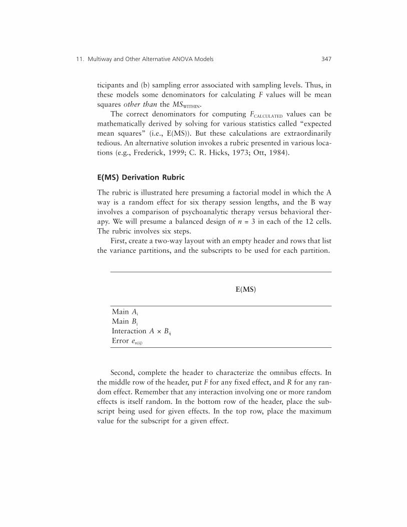
ticipants and (b) sampling error associated with sampling levels. Thus, inthese models some denominators for calculating F values will be meansquares other than the MSWITHIN.

The correct denominators for computing FCALCULATED values can bemathematically derived by solving for various statistics called “expectedmean squares” (i.e., E(MS)). But these calculations are extraordinarilytedious. An alternative solution invokes a rubric presented in various loca-tions (e.g., Frederick, 1999; C. R. Hicks, 1973; Ott, 1984).

E(MS) Derivation Rubric

The rubric is illustrated here presuming a factorial model in which the Away is a random effect for six therapy session lengths, and the B wayinvolves a comparison of psychoanalytic therapy versus behavioral ther-apy. We will presume a balanced design of n = 3 in each of the 12 cells.The rubric involves six steps.

First, create a two-way layout with an empty header and rows that listthe variance partitions, and the subscripts to be used for each partition.

E(MS)

Main Ai

Main Bj

Interaction A × Bij

Error en(ij)

Second, complete the header to characterize the omnibus effects. Inthe middle row of the header, put F for any fixed effect, and R for any ran-dom effect. Remember that any interaction involving one or more randomeffects is itself random. In the bottom row of the header, place the sub-script being used for given effects. In the top row, place the maximumvalue for the subscript for a given effect.


6 2 3R F R E(MS)i j n

Main Ai

Main Bj

Interaction A × Bij

Error en(ij)

Third, copy the number in the top row of the header to each of therows in that column only for rows in which the header subscript does notappear in the row label.


Main Ai 2 3Main Bj 6 3Interaction A × Bij 3Error en(ij)

Fourth, for any row with subscripts that are in parentheses, place a 1in the cell in the columns that are headed by a letter in the parentheses.


Main Ai 2 3Main Bj 6 3Interaction A × Bij 3Error en(ij) 1 1


Fifth, fill in the remaining empty cells of the layout. Put zeroes inempty cells for a fixed effect. Put 1s in empty cells for a random effect.


Main Ai 1 2 3Main Bj 6 0 3Interaction A × Bij 1 0 3Error en(ij) 1 1 1

Sixth, use the σ2 symbol for random-effects variance, and φ2 for fixed-effects variance. Enter σE

2 for the E(MS) for error. Next, for a given row,use a pencil, thumb, or finger to cover all columns with the row’s subscriptin the bottom row of the header only for row subscripts not in parentheses(e.g., for the Ai row, cover the first column, which has the subscript i; forthe en(ij) row, cover only the third column, which has the subscript n). So,for the A-way main effect, cover only the first of the three columns. Thenenter the uncovered weights for rows containing the i subscript and theassociated variance terms in the rightmost column. Of course, if anyuncovered column has a zero entry, the zero cancels out the variance fromthat source.


Main Ai 1 2 3 (2)(3)σA2 + (1)(1)σE

2

Main Bj 6 0 3Interaction A × Bij 1 0 3Error en(ij) 1 1 1 σE

2


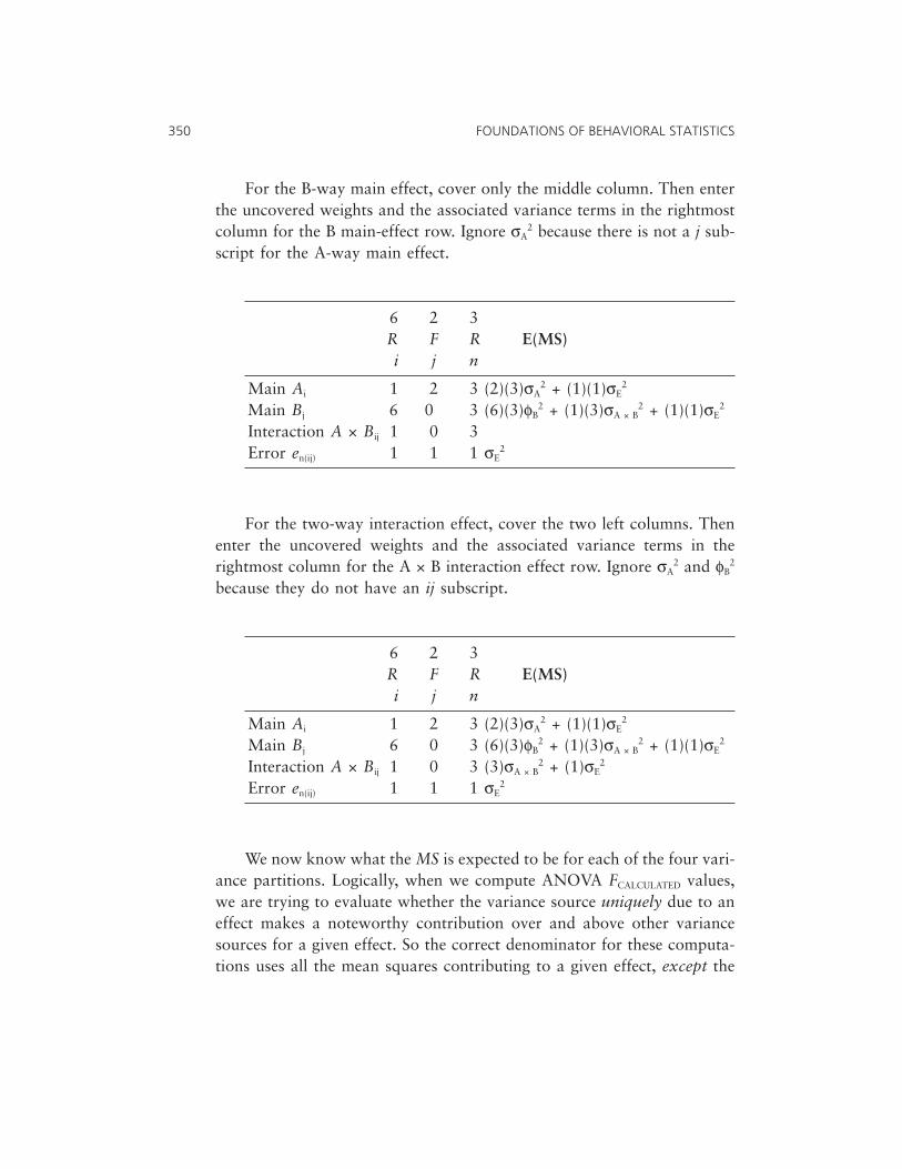
For the B-way main effect, cover only the middle column. Then enterthe uncovered weights and the associated variance terms in the rightmostcolumn for the B main-effect row. Ignore σA

2 because there is not a j sub-script for the A-way main effect.


Main Ai 1 2 3 (2)(3)σA2 + (1)(1)σE

2

Main Bj 6 0 3 (6)(3)φB2 + (1)(3)σA × B

2 + (1)(1)σE2

Interaction A × Bij 1 0 3Error en(ij) 1 1 1 σE

2

For the two-way interaction effect, cover the two left columns. Thenenter the uncovered weights and the associated variance terms in therightmost column for the A × B interaction effect row. Ignore σA

2 and φB2

because they do not have an ij subscript.


Main Ai 1 2 3 (2)(3)σA2 + (1)(1)σE

2

Main Bj 6 0 3 (6)(3)φB2 + (1)(3)σA × B

2 + (1)(1)σE2

Interaction A × Bij 1 0 3 (3)σA × B2 + (1)σE

2

Error en(ij) 1 1 1 σE2

We now know what the MS is expected to be for each of the four vari-ance partitions. Logically, when we compute ANOVA FCALCULATED values,we are trying to evaluate whether the variance source uniquely due to aneffect makes a noteworthy contribution over and above other variancesources for a given effect. So the correct denominator for these computa-tions uses all the mean squares contributing to a given effect, except the


variability uniquely due to the tested effect itself, as reflected in theE(MS)s.

For the A-way main effect, the E(MS) is 6σA2 + σE

2. To test the effectof variance contributed only from A, we are looking for a variance thatcontains all these variances except 6σA

2. The variance with this property isσE

2, the E(MS) for the error source. This means that when we are testingthe random-effect A way, we will compute the F by dividing MSA by theMSERROR.

For the B-way main effect, the E(MS) is 18φB2 + 3σA × B

2 + σE2. Again, to

test this main effect, we are looking for an E(MS) that contains all theseterms except 18φB

2. The E(MS) for the interaction term is 3σA × B2 + σE

2.This means that we will compute the FCALCULATED for the B main effect bydividing MSB by the MSA × B, instead of by the MSERROR.

For the interaction effect, the expected mean square is 3σA × B2 + σE

2.Because the only variance source in addition to the A × B interaction is theerror variance, we will compute the F test for this A × B interaction ran-dom effect by dividing MSA × B by the MSERROR.

Power versus Generality

To make this discussion concrete, Table 11.5 presents an hypotheticaldataset for our 6 × 2 mixed-effects model, in which the B way is treated asthe only fixed effect. Table 11.6 presents the ANOVA summary for themixed-effects model. Notice that the A-way main effect and the two-wayinteraction effects are both statistically significant, but that the B-waymain effect is not statistically significant.

For pedagogical purposes only—not as a model for the flexible andincorrect analytic practice of treating the same data by invoking contradic-tory models—Table 11.6 also presents a fixed-effects summary table forthe same data. As noted previously, the model employed does not changethe sums of squares, the degrees of freedom, or the mean squares. How-ever, the model selection does impact the denominator used in computingthe FCALCULATED values, and these changes in turn impact the correspondingpCALCULATED values. For our heuristic data, for the fixed-effects modelreported in Table 11.6, the pCALCULATED for the B way is 6E-8, but for themixed-effects model, the pCALCULATED for the B way is 0.301.

To summarize for the two-way case only, a fixed-effects model uses



TABLE 11.5. Illustrative Data for the Mixed-Effects Model

SPSS variable

Case DV A B

1 42 1 12 44 1 13 40 1 14 47 2 15 43 2 16 45 2 17 46 3 18 48 3 19 47 3 1

10 51 4 111 53 4 112 54 4 113 56 5 114 58 5 115 59 5 116 61 6 117 62 6 118 64 6 119 47 1 220 49 1 221 48 1 222 52 2 223 54 2 224 55 2 225 57 3 226 59 3 227 58 3 228 63 4 229 64 4 230 66 4 231 49 5 232 51 5 233 52 5 234 54 6 235 56 6 236 58 6 2

the MSWITHIN as the denominator for all three computations of theFCALCULATED values. For a random-effects model, the MSWITHIN is used as thedenominator only for the test of the two-way interaction effect, and theMSA × B is used as the denominator for both main effect tests. For a mixed-effects model the MSA × B is used to test the fixed-effect main effect, whilethe MSWITHIN is used to test both the random-effects main effect and theinteraction effect.

What impact does using a model other than the fixed-effects modelhave? As suggested by the heuristic comparisons in Table 11.6, the pres-ence of random effects within a model can reduce power against Type IIerror. So, the capacity to generalize beyond the levels actually used in ran-dom-effects ways may come at a cost.

None of this is to argue against treating effects as random. Indeed,some research problems almost cry out for this treatment (see Clark,1973). But the take-home message is to be thoughtful when makingthese decisions, because their consequences can be dramatic. Finally, itshould be noted that some modern statistical packages do not correctlyperform these calculations, so carefully review your computer results formixed-effects models.


TABLE 11.6. Summary Tables for Fixed- versus Mixed-Effects Models

Source SOS df MS FCALCULATED pCALCULATED

Fixed-effects model

A 883.56 5 176.71 73.122 9.9156E-14B 144.00 1 144.00 59.586 0.00000006A × B 542.00 5 108.40 44.855 2.0986E-11Error 58.00 24 2.42Total 1627.56 35 46.50

Mixed-effects model

A 883.56 5 176.71 73.122 9.9156E-14B 144.00 1 144.00 1.328 0.301A × B 542.00 5 108.40 44.855 2.0986E-11Error 58.00 24 2.42Total 1627.56 35 46.50

Note. The differences in entries for the two models are highlighted in bold.

�� Brief Comment on ANCOVA

In 1963, Campbell and Stanley wrote an influential chapter on experimen-tal and quasi-experimental design published in the Handbook of Researchon Teaching. The paperback reprint of this single chapter continues to bewidely used as a design textbook. In their chapter, Campbell and Stanley(1963, p. 193) recommended the use of a model called the analysis ofcovariance (ANCOVA), suggesting that “the use of this more precise anal-ysis [i.e., ANCOVA] would seem highly desirable.” They also argued that“covariance analysis and blocking on ‘subject variables’ such as priorgrades, test scores, parental occupation, etc., can be used, thus increasingthe power of the significance test” (p. 196).

ANCOVA can be roughly thought of as “in effect, an analysis of vari-ance performed [not on the Y scores, but] on the (Y – �Y)’s [or ei scores],where the �Y’s are predicted in the usual b1X + b0 [regression] way” (Glass& Stanley, 1970, p. 499), described in Chapter 8. Or, in Cliff’s (1987)words, “We could say that we are fitting a single regression equation tothe data for all the groups and then doing an anova of the deviation fromthe regression line [i.e., the ei scores]” (p. 275). Huitema (1980) and Loftinand Madison (1991) presented more detailed treatments of ANCOVA.

These linkages are intimated by the layout of the variance partitions inan ANCOVA summary table. Each main effect has degrees of freedomequal to the number of levels in a given way minus 1. In a factorial layout,each interaction effect is presented in a given row, with degrees of freedomequal to the product of the degrees of freedom for the relevant maineffects. And in the first row of the summary table, the covariates effect ispresented, with degrees of freedom equal to the number of covariates, justas would be the case in a regression summary table. The degrees of free-dom for covariates do not take into account group membership, becausegrouping is not considered within the covariance residualization portionof the analysis.

Some brief comments on using ANCOVA are warranted here, becauseas Keppel and Zedeck (1989) suggested,

It is somewhat depressing to note that while all statistical methodology bookscontinue to stress the conclusion that ANCOVA should not be used in quasi-


experimental designs [i.e., intact groups not randomly assigned], mis-applications of the procedure are still committed and reported in the litera-ture. (p. 482)

Three cautions about ANCOVA applications are presented here, with aparticular emphasis on the first concern (Thompson, 1992b).

Homogeneity of Regression Assumption Must Be Met

What ANCOVA actually does is to create a single regression equation,ignoring groups, to predict dependent variable (Yi) scores using thecovariate(s) (e.g., X1i, X2i, X3i). Then, in essence, an ANOVA, not ignor-ing groups, is performed using the residualized scores (ei) of each personcomputed by subtracting each person’s predicted score ( �Y), based on thesingle equation, from the participants’ actual scores (Yi).

These computations are legitimate iff the regression equations thatpredict the Yi scores, computed separately in the ANOVA groups, haveparallel slopes. This is the so-called homogeneity of regression assump-tion, which requires that the b weights applied to the covariate(s) are rea-sonably equal across each group. If this assumption is met, the use of asingle average, or “pooled” equation, for all the participants is unreason-able, creates e scores using a single regression equation that may not fit inany of the groups, and thus focuses the analysis on outcome scores (i.e., ei

scores) that are an inaccurate distortion for everybody.In education intervention studies, these slopes involving academic

achievement pretest covariates and posttest Y scores can actually be con-ceptualized as “rate of learning” curves. When the ANOVA groups werenot randomly created, but instead involved intact groups—especiallywhen one group was a compensatory group being given a remedial inter-vention such as Head Start—the homogeneity of regression assumptionmay be difficult, if not outright impossible, to meet.

Using ANCOVA to study intact groups may be appealing, becausewhen we have intact groups, especially in a compensatory intervention, werealize that the groups differed at pretest, and something must be done totake into account these pretest differences. Unfortunately, usingANCOVA in these situations may lead to “tragically misleading analyses”


that actually “can mistakenly make compensatory education look harm-ful” (Campbell & Erlebacher, 1975, p. 597). Similarly, Cliff (1987)argued that, “It could be that the relationship between the dependent vari-able and the covariate is different under different treatments. Such occur-rences tend to invalidate the interpretation of the simple partialcorrelations . . .” (p. 273).

Covariate(s) Data Must Be Extremely Reliable

Statistical corrections require extremely reliable measurement of the con-trol variables. Score reliability is an important requisite for any statisticalanalysis (Thompson, 2003), but “measurement reliability becomes crucial[emphasis added] . . . in employing statistical partialling operations, as inthe analysis of covariance . . .” (Nunnally, 1975, p. 10).

Unfortunately, too many researchers incorrectly presume that tests arereliable, and rarely check the reliabilities of the scores actually being ana-lyzed, as Vacha-Hasse, Henson, and Caruso (2002) reported in their mea-surement mega-meta-analysis. As Loftin and Madison (1991) emphasized,“the covariate(s) used must be especially reliable, or one will end uppotentially adjusting sampling error with measurement error, and creatinga mess” (p. 145).

Residualized Dependent Variable ScoresMust Be Interpretable

Some textbook authors have suggested that “adding covariates creates noreal problem” (Keppel & Zedeck, 1989, p. 479). But, on the contrary,some covariance corrections may result in the analysis of a dependent vari-able that no longer makes any sense.

Statistical corrections remove parts of the dependent variable, andthen analyze whatever is left, even if whatever is left no longer makes anysense. At some point we may no longer know what we are analyzing. AsThompson (1991b) suggested,

Consider an actual dissertation . . . in which the posttest [reading] achieve-ment variable was “corrected” using four pretest [reading] achievement


subtests. What was the posttest achievement variable after this correc-tion? . . . [W]hatever it was, this student probably wasn’t analyzing achieve-ment after this nuclear weapon covariance correction. (p. 508)

As Cliff (1987) explained, because “this [statistical correction] is really aform of regression, inferences become slipperier as the variables[covariates] increase” (p. 278) in number.

Some Key Concepts

Interaction effects are of considerable importance in social scienceresearch, because few if any interventions (e.g., instructional methods,drugs) work equally well for all people (Cronbach, 1957, 1975). ATIand related designs help us to determine for whom different interven-tions may be most effective.

Nonfactorial analyses exclude the testing of one or more omnibushypotheses. Researchers select nonfactorial analyses in some casesbecause a main effect may not be malleable, or because a higher-orderinteraction may not be readily interpretable. For some data, factorialanalyses have more power, but for other data, nonfactorial analysesare more powerful.

Just as people may be randomly sampled to yield generalizableresults, levels of ways may be randomly sampled in a random- ormixed-effects model. Such designs achieve greater generalizabilitybeyond the sampled levels, but due so at the cost of less statisticalpower for a given sample size.

ANCOVA is a statistical method that may be used to adjust sta-tistically for preintervention differences in groups. When enough par-ticipants are randomly assigned to groups in a true experiment, thelaw of large numbers functions efficiently, and such fine tuning willusually be unnecessary. When intact groups are used in a quasi-experiment (i.e., no random assignment to groups), adjustment forpreintervention differences may be desperately needed, but ANCOVAis less likely to be appropriate in exactly these cases. ANCOVArequires that the homogeneity of regression assumption is met, other-wise invoking a single regression equation across groups may result inadjustments that are inappropriate for all groups. The assumptionmay be most difficult to meet when the intact groups were createdusing eligibility rules (e.g., intervention is available only if academicperformance is at least one grade level below average) as part of com-pensatory or remedial efforts (Campbell & Erlebacher, 1975). Also,


the use of multiple covariates is possible, but may result in the analysisof an uninterpretable outcome variable.


1. In a balanced three-way ANOVA, all seven omnibus hypotheses are inher-

ently perfectly uncorrelated. This is worst-case as regards the

experimentwise error rate. What will αEXPERIMENTWISE be? What will hap-

pen to αEXPERIMENTWISE if a nonfactorial analysis is conducted?

2. Create hypothetical data for a balanced 3 × 2 design. For heuristic pur-

poses, use SPSS to analyze the data using (a) a fixed-effects model, (b) a

random-effects model, (c) a mixed-effects model with the A way declared

to be random and the B way declared to be fixed, and (d) a mixed-effects

model with the B way declared to be random and the A way declared to

be fixed. Which summary table entries are the same, and which differ

across the analyses? Do all the output results use the correct error terms

for the F calculations?


12

The GeneralLinear Model (GLM)

ANOVA via Regression

In one of his several seminal articles, Cohen (1968) noted that ANOVAand ANCOVA are special cases of multiple regression analysis, andargued that in these realizations “lie possibilities for more relevant andtherefore more powerful exploitation of research data” (p. 426). In a

book published shortly thereafter, Kerlinger and Pedhazur (1973) arguedthat multiple regression analysis

can be used equally well in experimental or non-experimental research. It canhandle continuous and categorical variables. It can handle two, three, four, ormore independent variables. . . . Finally, as we will abundantly show, multi-ple regression analysis can do anything the analysis of variance does—sumsof squares, mean squares, F ratios—and more. (p. 3)

Indeed, Maurice Tatsuoka (1975) noted that:

In the early writing of R. A. Fisher, the originator of ANOVA, it is evidentthat he initially approached the problem of multi-group significance testingvia the multiple linear regression method—which, as we shall soon see, isessentially what the [univariate] general linear model is. It was only (or at

359

least mainly) because the calculations needed for the multiple-regressionapproach were practically infeasible for all but the simplest designs in thepre-computer days, that Fisher invented the MSb/MSw approach. . . . [A]llconceivable designs in ANOVA and ANCOVA could be handled by a singlegeneral linear model, differing from design to design only in minute technicaldetail. (pp. 1–2)

The present chapter has two important foci: (a) presenting the basicconcepts of the general linear model (GLM), for the heuristic purpose ofshowing the linkages among statistical analyses, so that we may under-stand conceptually the similarities and the dissimilarities of these analyses,and (b) describing the practical reasons for using regression approaches inconducting the analysis of variance. The heuristic lessons of the chapterreinforce key messages that all analyses (a) are correlation, (b) yield effectsizes analogous to r2, and (c) apply weights to measured variables to yieldscores on latent variables that are actually the focus of the analysis.

Two implications of the GLM are, first, that effect sizes can (andshould) be presented and interpreted for all analyses. Second, althoughthere are important differences in experimental versus nonexperimentaldesigns (Raudenbush, 2005; Rubin, 1974), because all analyses are corre-lational and part of a single analytic family, there is no justification forunilaterally preferring ANOVA over other models. In particular, it will besuggested that the mutilation of intervally-scaled predictor variables intonominal scale in order to perform ANOVA generally should be avoided.

�� Planned Contrasts

Regression Subsumes ANOVA and the Two-Sample t Test

Table 12.1 presents a small one-way dataset that will be used to illustratethe fact that regression subsumes ANOVA (and by implication the two-sample t test) as a special case. This means that regression can be used toconduct ANOVA (or the two-sample t test, because for this problemtCALCULATED

2 = FCALCULATED), but not vice versa. These data are modeled onthe example provided by Tucker (1991).

For the purposes of this heuristic demonstration, we will use here the


five contrast variables, A1 through A5, as a set in place of the group mem-bership variable, LEVEL. These five variables merely reexpress exactly thesame information expressed in “LEVEL.” For example, saying that a par-ticipant had contrast variable scores of {–1, –1, –1, –1, –1} is merelyanother way of saying that a participant was in level 1 of the A way. Or,saying that a participant had contrast variable scores of {0, 0, 0, 0, 5} ismerely another way of saying that the participant was in level 6 of the Away. Indeed, the R2 (and R) of the five contrast variables with LEVEL is100%, reflecting the fact that the five contrast variables as a set contain nomore (and no less) information than that contained in LEVEL.

If we perform a regression analysis of these data using SPSS, we willobtain the summary table presented in Table 12.2. The relevant SPSS com-mand syntax is

REGRESSION VARIABLES=dv a1 a2 a3 a4 a5/DEPENDENT=dv/ENTER a1 a2 a3 a4 a5 .

This is exactly the same summary table that will result from performingANOVA using only the variables DV and LEVEL. Clearly, ANOVA can be

12. The General Linear Model (GLM) 361

TABLE 12.1. Orthogonal Contrast Variables for a One-Way ANOVA

SPSS variable names

Case DV LEVEL A1 A2 A3 A4 A5

1 11 1 –1 –1 –1 –1 –12 21 1 –1 –1 –1 –1 –13 10 2 1 –1 –1 –1 –14 20 2 1 –1 –1 –1 –15 10 3 0 2 –1 –1 –16 20 3 0 2 –1 –1 –17 10 4 0 0 3 –1 –18 20 4 0 0 3 –1 –19 10 5 0 0 0 4 –1

10 20 5 0 0 0 4 –111 31 6 0 0 0 0 512 41 6 0 0 0 0 5

Note. The six levels of the balanced (n in each cell is 2) one-way design are university academicclassifications: 1 = freshmen, 2 = sophomores, 3 = juniors, 4 = seniors, 5 = masters students,and 6 = doctoral students.

performed using regression, and is both (a) a special case of the univariateGLM, regression, and (b) is a correlational analysis, even though meandifferences are being tested.

This does not mean that regression can test only mean differences, butdoes mean that regression can be used to test mean differences. The notionthat there are two schools of analyses, experimental and correlational,died with Cohen’s (1968) article, if not with Cronbach’s (1957) presiden-tial address. There clearly are different research designs (Thompson et al.,2005), but univariate parametric analyses, such as ANOVA, ANCOVA,and t tests, are all special cases of multiple regression.

Testing Planned Contrasts

Aside from the important heuristic value of understanding that all analy-ses are correlational, yield r2-type effect sizes, and apply weights to mea-sured variables to estimate latent variable scores, there are also importantpractical reasons in some cases for conducting ANOVA via regression.The Table 12.1 data will also be used to illustrate this application.

In Chapter 10, I explained the use of omnibus ANOVA tests, followedby post hoc tests when necessary. The alternative ANOVA approacheschews entirely the use of either omnibus tests, or post hoc tests. Table12.3 presents the various synonyms used to refer to this alternative ana-lytic strategy.

Planned nontrend contrasts are variables created to test specifichypotheses about differences in means. In applied research, planned con-trasts are almost always created subject to the restriction that the contrast


TABLE 12.2. One-Way ANOVA Omnibus Test Summary Table


H0: µFr = µSo = µJr = µSr = µMa = µDoc 722.667 5 144.533 2.891 0.114 70.66%Within 300.000 6 50.000Total 1022.667 11 92.970

Note. “Fr” = freshmen, “So” = sophomores, “Jr” = juniors, “Sr” = seniors, “Ma” = masters, students; and“Doc” = doctoral students.

variables are perfectly uncorrelated. Orthogonal planned contrasts areuncorrelated variables created to test perfectly uncorrelated hypotheses.Another form of orthogonal planned contrasts, trend or polynomialorthogonal contrasts, will be explained momentarily.

Whenever any orthogonal planned contrasts are used, they partitionthe omnibus sum of squares for a main or interaction effect intononoverlapping variance partitions. Thus, because these partitions arenonoverlapping, the sum of the SOS partitions created using orthogonalplanned contrasts always exactly equals the omnibus SOS for a giveneffect. Thus planned contrasts provide more specific information aboutdynamics within ANOVA data, but do not change the overall effect sizesfor the omnibus effects.

Because planned contrasts do not require an omnibus test, we maytest interesting contrasts that might not be testable if an omnibus hypothe-sis was not rejected. And because when we use planned contrasts we donot test all possible simple or simple and complex contrasts, thus requiringa potentially large Bonferroni-type correction, planned contrasts can havemore power than post hoc tests. Planned contrasts do not require us to testcontrasts that are not of interest to us, or to lessen statistical power as theprice for conducting the full suite of post hoc comparisons.

For a given omnibus SOS, planned contrasts will cut this SOS intononoverlapping components, iff the planned contrast knives are orthogo-nal. Using orthogonal planned contrasts has the appealing feature thatnonoverlapping sums of squares simplifies our interpretation as to wherepredictive credit originates.


TABLE 12.3. Synonymous Namesfor Planned Contrasts

Phrase Elements

First Second

planned contrasta priori comparisonfocused test

Recall from Chapter 5 that

rXY = COVXY / (SDX * SDY) (5.1)

where COVXY is also a description of bivariate relationship, and can becomputed as

COVXY = (Σ(Xi – MX)(Yi – MY)) / (n – 1) (5.2)

Clearly, a necessary and sufficient condition for rXY to equal zero is forCOVXY to equal zero, as long as SDX and SDY are nonzero, such that rXY isdefined (i.e., can be computed). And the COVXY will equal zero as long asthe numerator of Equation 5.2, (Σ(Xi – MX)(Yi – MY)), equals zero.

Traditionally, contrast variables as tests of specific hypotheses are cre-ated such that their means (and sums) are zero. Thus, the contrast vari-ables are also deviation scores (as are any scores where M = 0), andEquation 5.2 can be rewritten as

COVXY = (Σ(xiyi)) / (n – 1) (5.3)

Moreover, COVXY and rXY will both be zero for any two variables forwhich Σ(xiyi) = 0.

As noted in Table 12.4, the 5 contrast variables all have means (andsums) of zero. Furthermore, the sums of the crossproducts for all 10pairwise combinations are all zero. This is illustrated in Table 12.4 for 5of the 10 possible pairwise combinations ([5(5 – 1)] / 2) of the 5 orthogo-nal planned contrasts. All deviation score crossproducts for the tabled 5pairs sum to zero.

Thus, all the planned contrasts in Table 12.1 are orthogonal(uncorrelated). Therefore, they will cut the omnibus SOS for the maineffect with df = 5 into five nonoverlapping sums of squares, each with 1degree of freedom. We can subdivide any omnibus sums of squares fur-ther, as long as the df of the omnibus effect is greater than 1. Once thedegrees of freedom for a variance partition equals 1, we cannot furthersubdivide the SOS information about individual differences.

What are the hypotheses tested by the tabled orthogonal nontrendcontrasts? In effect, we are applying the contrast variable scores to the


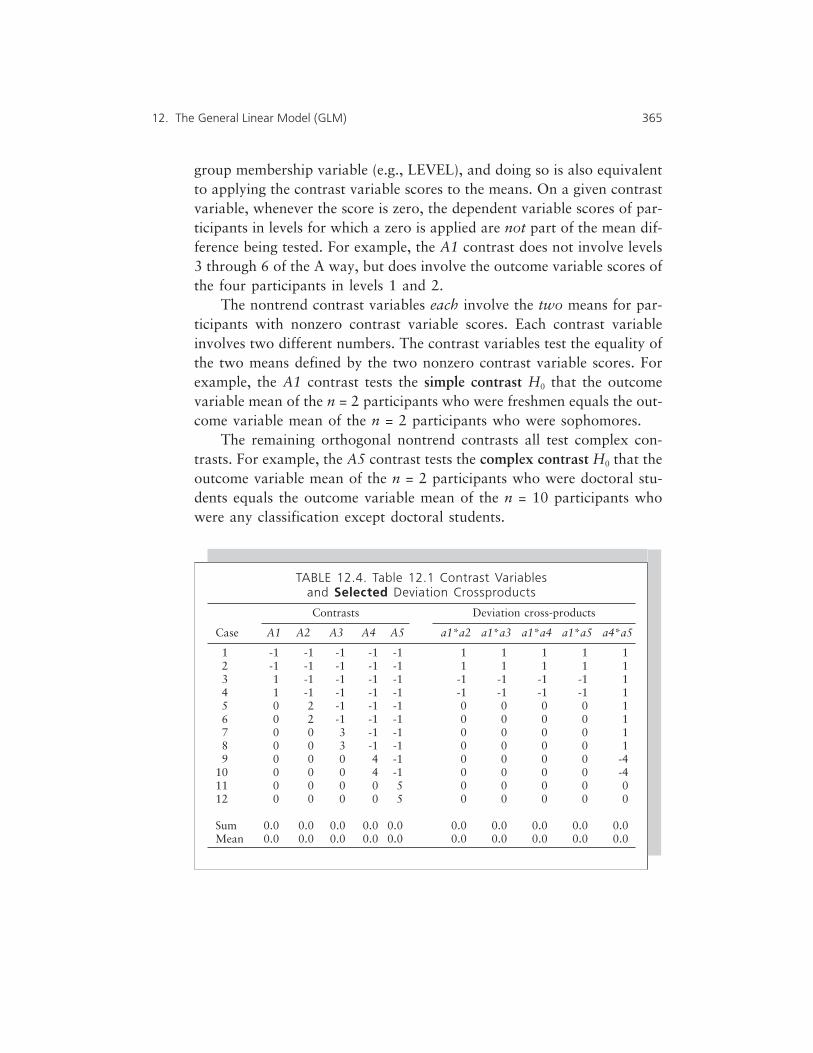
group membership variable (e.g., LEVEL), and doing so is also equivalentto applying the contrast variable scores to the means. On a given contrastvariable, whenever the score is zero, the dependent variable scores of par-ticipants in levels for which a zero is applied are not part of the mean dif-ference being tested. For example, the A1 contrast does not involve levels3 through 6 of the A way, but does involve the outcome variable scores ofthe four participants in levels 1 and 2.

The nontrend contrast variables each involve the two means for par-ticipants with nonzero contrast variable scores. Each contrast variableinvolves two different numbers. The contrast variables test the equality ofthe two means defined by the two nonzero contrast variable scores. Forexample, the A1 contrast tests the simple contrast H0 that the outcomevariable mean of the n = 2 participants who were freshmen equals the out-come variable mean of the n = 2 participants who were sophomores.

The remaining orthogonal nontrend contrasts all test complex con-trasts. For example, the A5 contrast tests the complex contrast H0 that theoutcome variable mean of the n = 2 participants who were doctoral stu-dents equals the outcome variable mean of the n = 10 participants whowere any classification except doctoral students.


TABLE 12.4. Table 12.1 Contrast Variablesand Selected Deviation Crossproducts

Contrasts Deviation cross-products

Case A1 A2 A3 A4 A5 a1*a2 a1*a3 a1*a4 a1*a5 a4*a5

1 -1 -1 -1 -1 -1 1 1 1 1 12 -1 -1 -1 -1 -1 1 1 1 1 13 1 -1 -1 -1 -1 -1 -1 -1 -1 14 1 -1 -1 -1 -1 -1 -1 -1 -1 15 0 2 -1 -1 -1 0 0 0 0 16 0 2 -1 -1 -1 0 0 0 0 17 0 0 3 -1 -1 0 0 0 0 18 0 0 3 -1 -1 0 0 0 0 19 0 0 0 4 -1 0 0 0 0 -4

10 0 0 0 4 -1 0 0 0 0 -411 0 0 0 0 5 0 0 0 0 012 0 0 0 0 5 0 0 0 0 0

Sum 0.0 0.0 0.0 0.0 0.0 0.0 0.0 0.0 0.0 0.0Mean 0.0 0.0 0.0 0.0 0.0 0.0 0.0 0.0 0.0 0.0

The planned contrasts are tested by executing the SPSS syntax:

REGRESSION VARIABLES=dv a1 a2 a3 a4 a5/DEPENDENT=dv/ENTER a1/ENTER a2/ENTER a3/

ENTER a4/ENTER a5 .

Note that because the planned contrasts are perfectly uncorrelated, theorder of entry into the regression model is irrelevant. The sum of squaresthat each contrast hypothesis will explain will be identical for any combi-nation of entry orders. However, the contrast hypotheses must be enteredone at a time, so that the unique explanatory contribution of each hypoth-esis can be determined.

Portions of the regression output are then consulted to use Excel, oranother spreadsheet, to build an ANOVA summary table. The sources inthe summary table at the outset can be listed as A1 (or H0: µFRESHMEN =µSOPHOMORES), A2 (or H0: µFRESHMEN, or SOPHOMORES = µSOPHOMORES)= µJUNIORS), A3,A4, A5, ERROR, and TOTAL. The degrees of freedom, known from themodel even before the analysis is conducted, are 1, 1, 1, 1, 1, 6, and 11,respectively.

At the entry of the first contrast variable, A1, the SOSREGRESSION is1.000 (reflecting the fact that the means of 16.0 and 15.0 are not equal).This SOS from the SPSS output is entered in the summary table for the A1contrast. At the entry of the second contrast variable, A2, the cumulativesum of squares explained is 1.333. This means that the SOS for the secondcontrast hypothesis alone is 0.333 (1.333 – 1.000). The sums of squaresfor the remaining contrast hypotheses are computed in an analogous man-ner, by subtraction.

After all the contrast variables are entered, the SOSERROR, the dfERROR,and the MSERROR are then correct, and can be read off the printout andentered into the spreadsheet. The SOSTOTAL can be computed at any entrypoint, because the SOSTOTAL is fixed for a given dataset.

Then the SPSS output is discarded, and the remaining entries in thesummary table are computed using Excel. The resulting summary table ispresented in Table 12.5. Notice that all we have done is to partition theomnibus SOS (i.e., 733.667 in Table 12.3) into five nonoverlapping com-ponents. And the SOSERROR and SOSTOTAL remain unaltered by the decision


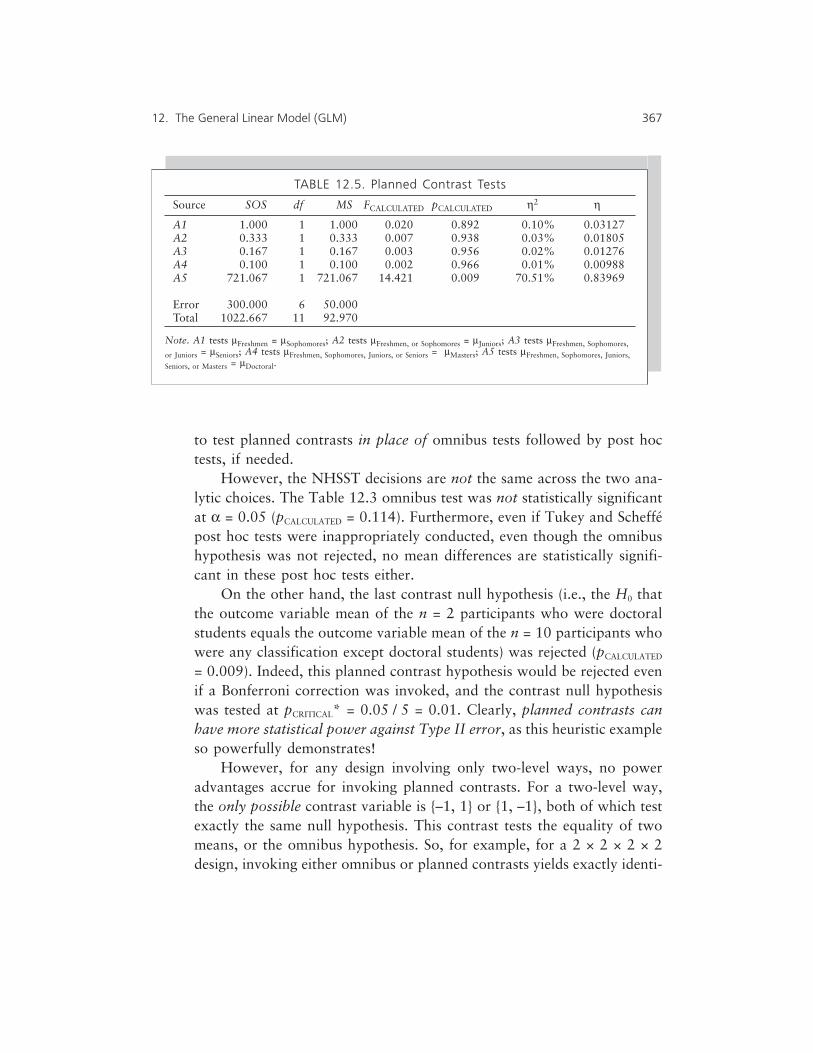
to test planned contrasts in place of omnibus tests followed by post hoctests, if needed.

However, the NHSST decisions are not the same across the two ana-lytic choices. The Table 12.3 omnibus test was not statistically significantat α = 0.05 (pCALCULATED = 0.114). Furthermore, even if Tukey and Scheffépost hoc tests were inappropriately conducted, even though the omnibushypothesis was not rejected, no mean differences are statistically signifi-cant in these post hoc tests either.

On the other hand, the last contrast null hypothesis (i.e., the H0 thatthe outcome variable mean of the n = 2 participants who were doctoralstudents equals the outcome variable mean of the n = 10 participants whowere any classification except doctoral students) was rejected (pCALCULATED

= 0.009). Indeed, this planned contrast hypothesis would be rejected evenif a Bonferroni correction was invoked, and the contrast null hypothesiswas tested at pCRITICAL* = 0.05 / 5 = 0.01. Clearly, planned contrasts canhave more statistical power against Type II error, as this heuristic exampleso powerfully demonstrates!

However, for any design involving only two-level ways, no poweradvantages accrue for invoking planned contrasts. For a two-level way,the only possible contrast variable is {–1, 1} or {1, –1}, both of which testexactly the same null hypothesis. This contrast tests the equality of twomeans, or the omnibus hypothesis. So, for example, for a 2 × 2 × 2 × 2design, invoking either omnibus or planned contrasts yields exactly identi-


TABLE 12.5. Planned Contrast Tests

Source SOS df MS FCALCULATED pCALCULATED η2 η

A1 1.000 1 1.000 0.020 0.892 0.10% 0.03127A2 0.333 1 0.333 0.007 0.938 0.03% 0.01805A3 0.167 1 0.167 0.003 0.956 0.02% 0.01276A4 0.100 1 0.100 0.002 0.966 0.01% 0.00988A5 721.067 1 721.067 14.421 0.009 70.51% 0.83969

Error 300.000 6 50.000Total 1022.667 11 92.970

Note. A1 tests µFreshmen = µSophomores; A2 tests µFreshmen, or Sophomores = µJuniors; A3 tests µFreshmen, Sophomores,

or Juniors = µSeniors; A4 tests µFreshmen, Sophomores, Juniors, or Seniors = µMasters; A5 tests µFreshmen, Sophomores, Juniors,

Seniors, or Masters = µDoctoral.

cal results for every effect in a factorial analysis. For this design, there areno power advantages (or disadvantages) for using a regression model toperform the analysis. And there are no choices about what hypotheses totest for each effect.

Nevertheless, in general, for research conducted on topics for whichprior research or theory, or both, can support reasonable expectations,planned contrasts may be very useful. First, if expectations pan out,planned contrasts have more power against Type II error, as illustrated inour example. Second, and perhaps more importantly, because the numberof planned orthogonal contrasts is capped for a main effect at k – 1,researchers must thoughtfully select the hypotheses they will test. Andthoughtfulness is absolutely the most critical ingredient in conductinghigh-quality scholarship.

Constructing Nontrend Planned Contrasts

We construct orthogonal planned contrasts for main effects such that thenumber of planned contrasts is less than or equals the number of groupsminus 1. One nontrend hypothesis tests a simple contrast, the second con-trast tests the mean outcome score of two groups versus the mean of athird group, and so forth.

We can create the nontrend contrasts in any order. For example, wemay be most certain that one group’s mean will differ from the combinedmean of all other participants, and we could define this complex contrastfirst. If this is the fifth contrast, we assign the one group contrast scores of5, and all other participants –1. In our example, the last contrast tested themean of group 6 versus the mean of everyone else combined. We couldinstead have used this contrast to test any one group (e.g., freshmen) ver-sus the remaining groups.

As we consecutively create the contrasts in any order, once we havecreated k – 2 contrasts, the last contrast is fixed. So we have no discretionin creating the last orthogonal nontrend contrast, whichever contrast weelect to create last.

Once the contrasts are selected, the contrast variables should havemeans (and sums) of zero, and the crossproducts of all pairs of contrastsshould sum to zero. The orthogonal nontrend contrasts should also have a


pattern in which the positive number equals the number of the contrastvariable. If we order the contrasts, as in Table 12.1, such that the simplecontrast is first, and the contrasts each successively involve one additionallevel, there will also be a pattern in which any participant with a nonzerocontrast variable score on a given contrast has –1 contrast scores on allcontrasts to the right of the given orthogonal nontrend contrast.

Logistically, there are two ways to create the contrast variable scoresin an SPSS analysis. First, we can literally type the contrast variable scoresinto the datafile. Second, we can input only dependent variable scores andgroup membership information for each way, and then invoke a series ofIF and COMPUTE statements to construct the contrast variable scores. Thiswill save us a lot of work, especially if we have a lot of participants in eachcell of the design.

Figure 12.1 provides the SPSS syntax used to analyze the Table 12.1data. Note that only the outcome variable scores (DV) and the groupmembership information for the single way (LEVEL) are input, and thatCOMPUTE and IF statements are used to create the orthogonal nontrendcontrasts.

Let’s consider another example. A researcher is conducting a bal-anced, factorial 4 × 3 ANOVA using nontrend contrasts. For a 4 × 3 facto-rial design, there will be a total of (4 × 3) – 1 degrees of freedom forexplained effects. Each contrast hypothesis requires 1 degree of freedom.So, for this model there will be 11 orthogonal nontrend contrast variables(i.e., cells minus 1, or [4 × 3] – 1).

Only the outcome scores (DEP_VAR) and cell information (WAY_Aand WAY_B) are input in the dataset. The contrast variables for the A waymight be created as

COMPUTE A1 = 0 .COMPUTE A2 = 0 .COMPUTE A3 = 0 .IF (WAY_A EQ 1) A1 = –1 .IF (WAY_A EQ 4) A1 = 1 .IF (A1 NE 0) A2 = –1 .IF (WAY_A EQ 3) A2 = 2 .IF (A2 NE 0) A3 = –1 .IF (WAY_A EQ 2) A3 = 3 .


The contrast variables for the B way might be created as

COMPUTE B1 = 0 .COMPUTE B2 = 0 .IF (WAY_B EQ 2) B1 = –1 .IF (WAY_B EQ 3) B1 = 1 .IF (B1 NE 0) B2 = –1 .IF (WAY_B EQ 1) B2 = 2 .


FIGURE 12.1. SPSS syntax used to analyze the Table 12.1 data

The orthogonal contrast variables for the interaction effects, requiring atotal of 6 degrees of freedom ([4 – 1][3 – 1]), can be created as

COMPUTE A1_B1 = A1 * B1 .COMPUTE A2_B1 = A2 * B1 .COMPUTE A3_B1 = A3 * B1 .COMPUTE A1_B2 = A1 * B2 .COMPUTE A2_B2 = A2 * B2 .COMPUTE A3_B2 = A3 * B2 .

Are these contrasts orthogonal? What hypotheses are tested by thefive main effect contrasts? You might benefit from creating hypotheticaloutcome variable scores for this problem, and then conducting the analy-sis using the REGRESSION procedure.

Selecting Nontrend Orthogonal Contrasts

The potentially greater power of planned contrasts is not an inherent func-tion of all planned contrasts. Instead, this power is a function of ourthoughtful selection of contrasts being informed by prior research, or the-ory, or both. Greater statistical power will not usually occur if plannedcontrasts are created randomly, or thoughtlessly.

One implication is that planned contrasts should not be used in newareas of inquiry where theory has not been elaborated. In such circum-stances, the use of omnibus tests followed by post hoc tests, if needed, isthe appropriate exploratory procedure. Thus, omnibus tests have animportant role in social science, even though planned contrasts can be veryuseful for some research problems.

The study by Carr and Thompson (1996) provided an example of theplanned contrasts model with an applied research problem. The research-ers were exploring the nature of reading learning disabilities. One modelposits that people with learning disabilities (LD) are not qualitatively dif-ferent from non-LD persons, and that disabilities merely reflect develop-mental delays.

The researchers reasoned from this perspective that (a) sixth-grade LDreaders should not differ substantially in reading proficiency from fourth-


grade non-LD readers, but (b) sixth-grade non-LD readers should differsubstantially in reading proficiency from both sixth-grade LD readers andfourth-grade non-LD readers. For this three-level one-way design, theresearchers used the nontrend orthogonal contrasts:

A1 A2 Group

–1 –1 sixth-grade LD readers1 –1 fourth-grade non-LD readers0 2 sixth-grade non-LD readers

In other words, the researchers expected (and obtained) small effectsizes and large pCALCULATED values for the A1 planned contrast. And theresearchers expected (and obtained) large effect sizes and small pCALCULATED

values for the A2 planned contrast. The beauty of the analysis is that theresearchers were able to test theoretical expectations about when effectsshould be small, as well as when effects should be large, all in the samestudy!

Using Bonferroni Corrections in a Planned Contrast Context

By tradition, researchers typically do not invoke the Bonferroni correctionwhen using orthogonal planned contrasts, even though experimentwiseerror rate inflation is at its maximum whenever the hypotheses beingtested are perfectly uncorrelated. The rationale for this decision involvesthe number of contrasts being tested.

In a six-level one-way design evaluating the omnibus hypothesis andthen post hoc tests, there are a huge number of simple and complex con-trasts being tested post hoc. Some correction for experimentwise error rateinflation seems essential when conducting post hoc tests, and the correc-tion is built into the Tukey or Scheffé post hoc analyses.

However, in the alternative analysis, a maximum of only five orthogo-nal planned contrasts can be conducted with this design. So, when plannedcontrasts are tested, experimentwise error rate inflation is somewhatcapped as a function of being limited to testing only a few contrasts. For amain effect, no more than k – 1 contrasts can be tested.


The fact that, traditionally, researchers do not invoke the Bonferronicorrection when testing planned contrasts does not mean that doing sowould be unreasonable. For more discussion of this issue, and on the useof nonorthogonal planned contrasts, see Thompson (1994c).

Using Latent Variable Scores in ANOVA

A brief comment on the implicit presence of weights and latent variables inANOVA is also warranted to flesh out the final general linear model link-ages of regression and ANOVA. The point is conceptual rather than anargument that estimating ANOVA �Y i scores usually has important practi-cal value.

Note that when we invoke orthogonal planned contrasts, we essen-tially are in a Case #1 regression situation (i.e., multiple, perfectly-uncorrelated predictors). And in Case #1, the beta weights for a regressionmodel equal the rs of each predictor with the Yi scores.

Table 12.5 presents the η2 and η values for each of the five orthogonalplanned contrast variables associated with the analysis of the Table 12.1data. As presented in the Figure 12.1 SPSS syntax, the Table 12.5 η valuesanalogous to r values can be used as β weights to compute the �Y i scores.

First, we reexpress the five orthogonal planned contrasts in z-scoreform. We can do this either by using COMPUTE statements, or by invokingthe SPSS command:

DESCRIPTIVES VARIABLES=dv a1 to a5/SAVE .

We then use the Table 12.5 η values as β weights in the syntax to createthe two ANOVA latent variable scores:

COMPUTE e = zdv – yhat .PRINT FORMATS yhat e (F8.5) .


COMPUTE yhat=(–.031270 * za1) + (–.018054 * za2) +(–.012766 * za3) + (–.009889 * za4) + (.839693 * za5) .

Table 12.6 presents the latent variable scores from this ANOVA.Remember that, in regression, the bivariate

rY × Y = RY × X1,X2 . . . (9.3)

and equivalently that

rY × Y2 = RY × X1,X2 . . .

2 (9.4)

which suggests an analogous linkage elsewhere in the general linearmodel. If we use the SPSS CORRELATIONS command to obtain the Pearsonproduct–moment correlation between the ZDV (or the DV scores) and theANOVA YHAT scores, we obtain r = 0.8406. As expected, the squaredvalue of this correlation coefficient, 0.84062 = 70.66%, equals the omni-bus ANOVA η2 (i.e., 722.67 / 1022.67 = 70.66%), as reported in Table12.2.

Furthermore, for regression we learned that the SOS of the �Y i scoresequals the SOSEXPLAINED. The same truism applies in ANOVA. Here we are


TABLE 12.6. Latent Variable Scores for the Table 12.1 ANOVA Data

SPSS variable

Case/statistic DV ZDV YHAT E

1 11 –0.795 –0.276 –0.5182 21 0.242 –0.276 0.5183 10 –0.899 –0.380 –0.5184 20 0.138 –0.380 0.5185 10 –0.899 –0.380 –0.5186 20 0.138 –0.380 0.5187 10 –0.899 –0.380 –0.5188 20 0.138 –0.380 0.5189 10 –0.899 –0.380 –0.518

10 20 0.138 –0.380 0.51811 31 1.279 1.798 –0.51812 41 2.316 1.798 0.518

M 18.667 0.000 0.000 0.000SOS 1022.667 11.000 7.773 3.220SD2 92.970 1.000 0.707 0.293SD 9.642 1.000 0.841 0.541

using β weights, so we are predicting zY rather than Yi scores. The SOS ofthe n = 12 zY scores is, of course, 11.000, as reported in Table 12.6. TheSOS of the ANOVA �Y i scores, reported in Table 12.6, is 7.773. The omni-bus ANOVA η2 (i.e., 70.66%) reported in Table 12.2 also equals 7.773 /1.000, as expected.

�� Trend/Polynomial Planned Contrasts

In the special case in which (a) a way is quantitative and (b) the levels areequally spaced, researchers may elect to use trend or polynomial contrasts.Nontrend planned contrasts test whether two means are equal. Trend/polynomial planned contrasts do not each test whether two means areequal but instead test whether the means across the levels form a certainpattern (e.g., a line, a parabola).

In a two-way design, if both the A way and the B way are quantitativeand their levels are equally spaced, trend contrasts can be used with the Away only, with the B way only, with both, or with neither. And if trendcontrasts are used for either or both ways, all the contrast variables,including those for interaction effects, will be uncorrelated as long as thedesign is balanced.

Table 12.7 presents orthogonal polynomial contrasts that can be usedwith a three-level, four-level, or five-level way. Contrasts are not presentedfor a two-level way, because for a two-level way only one contrast is possi-ble, and that contrast must test the omnibus hypothesis. Also, a two-levelway cannot create patterns of means other than a line, even if the way isquantitative and the levels are equally spaced, because two points inher-ently define a line, and no nonlinear patterns can be created by only twopoints in a Cartesian space. The interested reader will confirm that thetabled contrasts are orthogonal.

Figure 12.2 presents a plot of the patterns being tested by the fourorthogonal polynomial contrasts for a five-level way. The linear contrast,{–2, –1, 0, 1, 2}, defines a straight line in Figure 12.2. The quadratic con-trast, {2, –1, –2, –1, 2}, creates a parabola with one bend, in the middle ofthe plot. The cubic contrast, {–1, 2, 0, –2, 1}, defines a line with twobends, both equidistant from the boundaries of the plot. The quartic con-


trast, {1, –4, 6, –4, 1}, defines a line with three bends, or a shape resem-bling the letter W.

When we are fitting orthogonal trend contrasts to our data, we aretesting the fit of the pattern of the contrast to the fit of the pattern in themeans on the quantitative way. For example, the study might involve anoutcome of psychological adjustment, with the way being five equidistantdurations of therapy sessions (e.g., 40, 45, 50, 55, and 60 minutes). Or,the study might involve a drug dosage investigation with an outcome ofthe joint mobility of arthritis patients, each given either 500, 600, 700,800, or 900 milligrams of aspirin. We are interested in seeing whether


TABLE 12.7. Selected Polynomial/Trend Orthogonal Contrasts

Levels

Levels Contrast 1 2 3 4 5

3 Linear –1 0 1Quadratic 1 –2 1

4 Linear –3 –1 1 3Quadratic 1 –1 –1 1Cubic –1 3 –3 1

5 Linear –2 –1 0 1 2Quadratic 2 –1 –2 –1 2Cubic –1 2 0 –2 1Quartic 1 –4 6 –4 1

FIGURE 12.2. Plots of polynomial contrast variables for a five-level way

greater dosages linearly produce successively smaller or larger outcomemeans, or whether there are curvilinear reaction patterns across dosages.

When we use the linear contrast variable, which is an upward slopingline in Figure 12.2, we are not testing whether the means define an upwardsloping line with a given slope, or even an upward versus a downwardsloping line. Instead, we are testing whether the pattern of the means hasthe same basic character (not direction or orientation) as the polynomialcontrast. So, the linear contrast tests whether the means either progres-sively and incrementally go up, or progressively and incrementally godown.

By the same token, the quadratic pattern in Figure 12.2 defines a Vshape. But the quadratic contrast is not testing whether the pattern of themeans has this particular V shape, or indeed any V shape. Instead, we aretesting whether the pattern of the means either (a) goes down, and corre-spondingly then up, with the single pattern bend in the middle, or (b) goesup, and correspondingly then down, again with the single pattern bend inthe middle.

Table 12.8 presents a heuristic dataset for a five-level quantitativeway. For these data, the means have the pattern of {10, 20, 30, 25, 20}.Here we will test whether the means create a linear, a quadratic, or someother pattern. For heuristic purposes, we will not break the omnibus sumof squares into four subcomponents; instead we will break the omnibusSOSEXPLAINED only into three subcomponents, one of which will have twodegrees of freedom. Of course, for comparative purposes, you are encour-aged to perform an alternative analysis with all four possible orthogonalpolynomial contrasts.

Table 12.9 presents the results from an omnibus ANOVA test. Thistable is presented only for heuristic comparative purposes. In actualresearch, one always uses either omnibus tests with post hoc tests, ifneeded, or planned contrasts. However, the Table 12.9 omnibus resultswill later be used to confirm that the planned contrast analysis does notimpact the error or total variance partitions, and only subdivides theSOSEXPLAINED into nonoverlapping sums of squares associated with eachtested pattern of the five means.


We conduct the analysis the same way we conducted the analysis forthe nontrend orthogonal contrasts. We can use the SPSS syntax:

ENTER linear/ENTER quadratc/ENTER cubic quartic .

We use the output to compute the five sums of squares of interest in ouranalysis. For example, the SOSLINEAR, after the linear contrast variable isentered, is 187.50. After the quadratic contrast is entered second, we con-


REGRESSION VARIABLES=dv linear quadratc cubic quartic/

TABLE 12.8. Orthogonal Polynomial Datafor One-Way Five-Level ANOVA

SPSS variable names

Case DV LEVEL LINEAR QUADRATIC CUBIC QUARTIC

1 9 1 –2 2 –1 12 10 1 –2 2 –1 13 11 1 –2 2 –1 14 19 2 –1 –1 2 –45 20 2 –1 –1 2 –46 21 2 –1 –1 2 –47 29 3 0 –2 0 68 30 3 0 –2 0 69 31 3 0 –2 0 6

10 24 4 1 –1 –2 –411 25 4 1 –1 –2 –412 26 4 1 –1 –2 –413 19 5 2 2 1 114 20 5 2 2 1 115 21 5 2 2 1 1

TABLE 12.9. One-Way ANOVA Omnibus Test of Table 12.6 Data


Between 660.00 4 165.00 165.00 0.000000004 98.51%Within 10.00 10 1.00Total 670.00 14 47.86

sult the output and perform a subtraction of the cumulative SOSEXPLAINED

minus the SOSLINEAR to determine the SOSQUADRATIC, which is 433.93.After the sums of squares are computed, we then use Excel to compute

the remaining elements of the required summary table. Table 12.10 pres-ents the summary table for these data.

One heuristic digression may be worthwhile. For these data, when theoutcome variable is intervally-scaled, so, too, is the quantitative way.Therefore, for this special ANOVA case, we could compute the Pearsonproduct–moment r2 between the outcome variable and the levels of thequantitative way, using the SPSS CORRELATIONS procedure. Doing soyields r = 0.5290. The r2 value (i.e., 0.52902 = 27.98%) is remarkably sim-ilar (i.e., identical) to the η2 value (27.98%) reported for the linear con-trast in Table 12.10.

The comparison makes two heuristic points. First, the linear contrasttests for only linear patterns, and the Pearson r only measures linear rela-tionship, so of course we expect this correspondence. Second, the omnibusη2 (98.51%) is sensitive to all forms of relationship, which is why theomnibus η2 is greater than the r2. Linear relationship is only one form ofrelationship. Thus, η2 = 98.51% includes the linear component (i.e.,27.98%), but also all other relationship forms (i.e., 27.98% + 64.77% +5.76% = 98.51%).

For this hypothetical, small dataset, the effect sizes are huge (i.e.,cumulatively, almost perfect). Nevertheless, the example illustrates thebest fit of the quadratic effect. Assuming the outcome scores are scaledsuch that higher scores are better, such a pattern suggests an optimal dos-age located near the middle treatment level used in the way. If this wayinvolved a study of therapy session durations of 40, 45, 50, 55, and 60minutes, the result would suggest an optimal session length of 50 minutes.


TABLE 12.10. Polynomial Trend Tests of Table 12.6 Data


Linear 187.50 1 187.50 187.50 0.000000083 27.98%Quadratic 433.93 1 433.93 433.93 0.000000001 64.77%Other 38.57 2 19.29 19.29 0.000369909 5.76%Within 10.00 10 1.00Total 670.00 14 47.86

Of course, the effect sizes we have considered are always on the aver-age. (For an interesting exception, see Grissom, 1994.) Effect sizes (unlessthey are perfect) do not mean that the effect was consistent for all partici-pants. A large but imperfect effect means that an intervention generallyworked in a given fashion for the group as a whole, but for some partici-pants the optimal treatment may not be as effective, and may even be leasteffective.

�� Repeated-Measures ANOVA via Regression

Repeated-measures ANOVA designs repeatedly (at least twice) measureparticipants on one or more outcome variables over time. For example, adrug study might be conducted to evaluate the effects of threeanticholesterol drugs. In a between-subjects design, in which a given par-ticipant is involved in only one level of the way, 90 participants (30 pergroup) might be randomly assigned to take only one of the three drugs fora month, after which outcome cholesterol scores would be recorded.Alternatively, in a within-subjects (or repeated measures) design, 30 partic-ipants would each successively receive each drug, and have cholesteroloutcome scores recorded, over the course of the study.

For example, the three drugs might be administered in a counterbal-anced order to subgroups of participants. Ten participants might receivedrug A during January, drug B during March, and drug C during May,having their cholesterol recorded at the end of January, March, and May.Ten other participants might receive drug B during January, drug C duringMarch, and drug A during May, having their cholesterol recorded at theend of each month. Finally, 10 other participants might receive drug Cduring January, drug A during March, and drug B during May, havingtheir cholesterol recorded at the end of each month.

Repeated measures may have two appealing features. First, we may beable to record the same number of outcome scores (e.g., 30 per drug) witha repeated-measures design that requires fewer participants than abetween-subjects design (e.g., 30 versus 90 participants). Second,repeated-measures designs have the appealing feature that each participantmay be exposed to each treatment. This may be important, particularly if


the sample size is small and includes one or more atypical people. Theinfluence of outliers may be minimized either by (a) washing out theseinfluences within a large sample, or (b) including the outliers in everytreatment condition so that outliers do not distort outcome means only forcertain conditions to which they were assigned.

The key issue in deciding whether a repeated-measures design isappropriate in a given study involves whether or not the performances ofthe participants over time are reasonably independent. For example, in acholesterol study, with drugs administered every other month over a 5-month period and with 1 month of no treatment separating the drugadministrations, there is probably not much reason to expect carryovereffects across drug treatments.

But what if the study was an educational intervention designed toteach first graders how to spell 10 target words? Once a child receives anyinstruction, and learns some of the target words, the prior learning willcompromise the ability to detect new impacts when the same words areretaught. Nevertheless, for some research, repeated-measures designs canbe quite useful.

Table 12.11 presents a heuristic dataset for the simplest possiblerepeated-measures design. A multiway repeated-measures design mightinvolve a within-subjects effect, and one or more between-subjects effectsfor which people by choice are not, or simply cannot be, assigned succes-sively to each condition (e.g., two genders). Here there is only one within-subjects effect, and no between-subjects effects. Let’s say Table 12.11


TABLE 12.11. Repeated-Measures ANOVA Data

Test

Participant/statistic 1 2 3 4 Sum Mean

1 5 7 7 8 27 6.752 4 5 8 9 26 6.503 4 4 4 8 20 5.004 3 3 4 8 18 4.505 2 2 4 5 13 3.25

Sum 18 21 27 38Mean 3.60 4.20 5.40 7.60 5.20

involves giving five participants therapy for four weeks, and measuringpsychological adjustment at the end of each week.

We could enter the data into SPSS as a file containing five rows andfour outcome variable scores, T1, T2, T3, and T4, arrayed as the data arewithin Table 12.11 but entering only these 5 × 4 = 20 data points. Therequired SPSS syntax to yield a repeated-measures ANOVA would be

MANOVA t1 t2 t3 t4/WSFACTORS test(4)/PRINT=SIGNIF(UNIV MULTIV AVERF HF GG EFSIZE)PARAM(ESTIM)/WSDESIGN=test/DESIGN .

Alternatively, if we wish, we can conduct the repeated-measuresANOVA using regression. And because the four measurements are quanti-tative (i.e., time) and equally spaced (i.e., weekly), here we can conduct theanalysis using orthogonal polynomial planned contrasts. The data areentered as 20 rows, in the format presented in Table 12.12. Using themethod first suggested by Pedhazur (1977), we also enter the sum of eachparticipant’s four outcome variable scores (e.g., Σ1 = 5 + 7 + 7 + 8 = 27) inevery row for a given participant.

We implement the analysis in SPSS, using the syntax

REGRESSION VARIABLES=dv linear quadratc cubic sum/DEPENDENT=dv/ENTER sum/ENTER linear/ENTER quadratc/ENTER cubic .

As before, we use elements from the output to create the summary table inExcel. The SOSPEOPLE is derived from the entry of the variable “SUM” intothe model. This sum of squares (33.70) reflects the variability within dif-ferent people across the four measurements.

The cumulative SOS after “LINEAR” is entered is 77.26, whichmeans that the SOS for the linear pattern in the four outcome means is43.56 (i.e., 77.26 – 33.70). By successive subtractions, we computeSOSQUADRATIC to be 3.20, and SOSCUBIC to be 0.04. The residual, or people× time interaction SOS, is 10.70. After entering these values into Excel, wediscard the SPSS output, and compute the remaining entries in the sum-


mary table, yielding the results reported in Table 12.13. For a relatedexample, see Edwards (1985, Ch. 10).

One complication is that we have not taken into account an importantstatistical assumption. The sphericity assumption requires that the vari-ances of the differences between all possible pairs of means must be equal.The F test (and associated pCALCULATED values) will be inaccurate to theextent that we violate this assumption.

The initial repeated-measures ANOVA presumes that data perfectlymeet the sphericity assumption. We can attempt to quantify the extent towhich we are violating this assumption, and then use this estimate, calledepsilon (ε), to obtain more accurate pCALCULATED values. One estimate of ε isthe Geisser-Greenhouse correction (Geisser & Greenhouse, 1958), whichis provided by SPSS upon request. For our data, εGG = 0.721. Another esti-mate was developed by Huynh and Feldt (1976). For our data, εHF =1.000.


TABLE 12.12. Repeated-Measures Data with Polynomial Contrasts

SPSS variable names

Row CASE TEST LINEAR QUADRATC CUBIC SUM DV

1 1 1 –3 1 –1 27 52 2 1 –3 1 –1 26 43 3 1 –3 1 –1 20 44 4 1 –3 1 –1 18 35 5 1 –3 1 –1 13 26 1 2 –1 –1 3 27 77 2 2 –1 –1 3 26 58 3 2 –1 –1 3 20 49 4 2 –1 –1 3 18 3

10 5 2 –1 –1 3 13 211 1 3 1 –1 –3 27 712 2 3 1 –1 –3 26 813 3 3 1 –1 –3 20 414 4 3 1 –1 –3 18 415 5 3 1 –1 –3 13 416 1 4 3 1 1 27 817 2 4 3 1 1 26 918 3 4 3 1 1 20 819 4 4 3 1 1 18 820 5 4 3 1 1 13 5

The ε values are used to adjust the degrees of freedom when comput-ing pCALCULATED values from the FCALCULATED results, subject to the restrictionthat the adjusted dfNUMERATOR not be less than 1 and the adjusteddfDENOMINATOR not be less than the number of participants. For our data, theuncorrected pCALCULATED value for the linear effect was obtained in Excel byinputting the F of 48.85 with degrees of freedom 1 and 12:

=FDIST(48.85,1,12)

which yields a pCALCULATED value of 0.00001.However, if we invoke the Geisser-Greenhouse correction, we instead

input

=FDIST(48.85,1,.721*12)

or, alternatively,

=FDIST(48.85,1,8.652)

and obtain a pCALCULATED value of 0.00011. But for our example, invokingεHF yields the same pCALCULATED results as the uncorrected results, becauseour εHF = 1.000.


TABLE 12.13. Summary Table for Repeated-MeasuresANOVA with Planned Polynomial Contrasts


People 33.70 4 8.42Time 46.80 3 15.60

Linear 43.56 1 43.56 48.85 0.00001 47.76%Quadratic 3.20 1 3.20 3.59 0.08252 3.51%Cubic 0.04 1 0.04 0.04 0.83582 0.04%Within Time (Total – Time) 44.40

People × Time (Within – People) 10.70 12 0.89Total 91.20 19

Note. The omnibus hypothesis is not tested when planned contrasts are performed, but for heuristicpurposes note that the omnibus FCALCULATED is 17.50 (p = 0.0001).

The εGG is generally lower than εHF, and thus results in a larger correc-tion of degrees of freedom (i.e., fewer degrees of freedom), less poweragainst Type II error, and larger pCALCULATED values. Some researchers havesuggested computing ε as an average of εGG and εHF (e.g., J. Stevens, 1996).Others (cf. Girden, 1992) have suggested using εHF iff εGG is larger than0.75. For more detail on these decisions, see Tanguma (1999).

Our results suggest a linear effect of therapy over time. Of course, ourconclusions must be limited to 4 weeks of treatment. Our design will notallow us to conclude that longer durations of therapy will necessarily con-tinue to lead to incremental improvements in mental health. Our resultsalso suggest that individual differences due to people (i.e., SOSPEOPLE =33.70) are noteworthy. We can only estimate these person effects by usinga repeated-measures design in which individuals are measured repeatedly.

�� GLM Lessons

Analysis of variance (ANOVA) has traditionally been among the mostcommonly used of all inferential statistical techniques in the behavioralsciences (Edgington, 1974; Wick & Dirkes, 1973), though a growing trendfavoring the use of regression and general linear model methods hasemerged (Kieffer, Reese, & Thompson, 2001) since Cohen’s (1968) influ-ential article.

Edgington (1974) reviewed American Psychological Associationresearch journals and found that 71% of the articles using statistical infer-ence had employed analysis of variance. He concluded his review by not-ing that “. . . every one of the journals showed an upward trend in the useof analysis of variance . . .” (p. 26). Willson (1980) proposed that theremight be a change in techniques used in research articles publishedbetween 1969 and 1978, due to the expansion of educational researchtraining in the late 1960s. He examined the articles published in AmericanEducational Research Journal (AERJ) from 1969 to 1978, and he foundlittle extension of the research tools used—ANOVA and ANCOVA wereincluded in 56% of the articles.

Goodwin and Goodwin (1985) found that the total percentage ofusage for ANOVA-based techniques decreased to 34.47% in the 189 arti-


cles that were published in AERJ from 1979 to 1983. Elmore andWoehlke (1988) found that ANOVA/ANCOVA were still the most fre-quent research methods utilized in all articles appearing in AERJ, Educa-tional Researcher, and Review of Educational Research from 1978 to1987.

Take-Home Messages

In this chapter, several arguments have been presented. First, regressionapproaches to ANOVA that invoke planned contrasts have been recom-mended for many designs in which one or more ways have more than twolevels. Planned contrasts (a) may have more power against Type II error, iffresearchers have a reasonable basis for formulating specific, nonomnibushypotheses, and (b) tend to force researchers to thoughtfully selecthypotheses as against testing every possible mean difference. Second,omnibus tests followed by post hoc tests, if needed, are perfectly appropri-ate for research situations in which prior research or theory is not avail-able.

We will now turn to a major, third implication of the heuristic demon-stration that ANOVA and the two-sample t test are special cases of theunivariate general linear model (i.e., multiple regression). Because all anal-yses are correlational, ANOVA and regression are part of one GLM, so donot fall prey to the tendency to mutilate intervally-scaled predictors tonominal scale merely so that ANOVA methods can then be used.

Mutilating Intervally-Scaled Independent Variables

One reason why researchers may be prone to categorizing continuousvariables (i.e., converting intervally scaled variables down to nominalscale) is that some researchers unconsciously and erroneously associateANOVA with the power of experimental designs. Researchers often valuethe ability of experiments to provide information about causality (Thomp-son et al., 2005); they know that ANOVA can be useful when independentvariables are inherently nominally-scaled and dependent variables areintervally-scaled; they then begin to unconsciously identify the analysis ofANOVA with the design of an experiment.


It is one thing to employ ANOVA when an experimental design is infact used. However, it is something quite different to assume that causalinferences can be made just because an ANOVA is performed. This illogic,in which design and analysis are confused with each other, are all the morepernicious, because the confusion tends to arise unconsciously and thus isnot readily perceived by the researcher (Cohen, 1968).

Humphreys (1978) noted that:

The basic fact is that a measure of individual differences is not an indepen-dent variable, and it does not become one by categorizing the scores andtreating the categories as if they defined a variable under experimental con-trol in a factorially designed analysis of variance. (p. 873)

Similarly, Humphreys and Fleishman (1974) noted that categorizing vari-ables in a nonexperimental design using an ANOVA analysis “not infre-quently produces in both the investigator and his audience the illusion thathe has experimental control over the independent variable. Nothing couldbe more wrong” (p. 468).

These sorts of confusion are especially disturbing when the researcherhas some independent or predictor variables that are intervally-scaled (e.g.,pretest IQ scores), and converts them to nominal scale (e.g., low IQ, highIQ), just to be able to perform some ANOVA analysis. As Cliff (1987) noted,the practice of discarding variance on intervally-scaled predictor variables toperform OVA analyses creates problems in almost all cases:

Such divisions are not infallible; think of the persons near the borders. Somewho should be highs are actually classified as lows, and vice versa. In addi-tion, the “barely highs” are classified the same as the “very highs,” eventhough they are different. (p. 130)

Moreover, not enough researchers realize that the practice of discard-ing variance on an intervally-scaled predictor variable to perform OVAanalyses from a score reliability or measurement point of view “makes thevariable more unreliable, not less” (Cliff, 1987, p. 130), which in turnlessens statistical power against Type II error. Pedhazur (1982) made thesame point, and explicitly presented the ultimate consequences of badpractice in this vein:


Categorization of attribute variables is all too frequently resorted to in thesocial sciences. . . . It is possible that some of the conflicting evidence in theresearch literature of a given area may be attributed to the practice of catego-rization of continuous variables. . . . Categorization leads to a loss of infor-mation, and consequently to a less sensitive analysis. (pp. 452–453)

It is the IQ dichotomy or trichotomy in the computer, and not theintervally-scaled IQ data with a Cronbach’s α reliability of 0.93 sitting andcollecting dust on the shelf, that will be reflected in the ANOVA results.

Score variability is the “stuff” (i.e., information about the amount andorigins of individual differences) on which all analyses are based. Dis-carding variance by categorizing variables amounts to “squandering ofinformation” (Cohen, 1968, p. 441). As Kerlinger (1986) explained,

partitioning a continuous variable into a dichotomy or trichotomy throwsinformation away. . . . To reduce a set of values with a relatively wide rangeto a dichotomy is to reduce its variance and thus its possible correlation withother variables. A good rule of research data analysis, therefore, is: Do notreduce continuous variables to partitioned variables (dichotomies,trichotomies, etc.) unless compelled to do so by circumstances or the natureof the data (seriously skewed, bimodal, etc.). (p. 558)

The conversion of interval predictor variables into dichotomies ortrichotomies distorts (a) the distribution shape of the converted variablesin relation to the distribution we believe the variables have in the realitywe purportedly wish to study; (b) the variability of the converted variableby discarding variance we believe exists in the reality we purportedly wishto study; and (c) the relationships among predictors by making all predic-tors perfectly uncorrelated when a balanced ANOVA is performed, thusdishonoring a reality in which variables are usually correlated (Hester,2000; Thompson, 1986, 1988a). This last feature of ANOVA, as Cohen(1968) pointed out, vastly simplifies the calculation process, which wasimportant in the 1920s, but hardly seems a worthy sacrifice when a micro-computer can perform calculations in seconds without requiring suchcomputational simplifications.

Of course, ANOVA does remain a useful tool when the independentvariables are all inherently nominal (e.g., dichotomies or trichotomies,such as assignment to experimental condition or gender). However, in


many areas of inquiry, relatively few independent variables are inherentlynominally-scaled, and so in many cases using ANOVA may raise ques-tions about distorting data.

Three Possible Data Mutilation Scenarios

Three potential scenarios can be envisioned for data mutilation. First, anindependent variable (e.g., pretest standardized test scores, pretest IQscores) may be intervally-scaled with considerable variability, and perhapseven a normal distribution. In this scenario, converting the scores into adichotomy or a trichotomy (a) discards score variability, which in turn (b)reduces score reliability, (c) distorts score shape by converting a normaldistribution into a uniform/rectangular distribution, and (d) alters rela-tionships with other variables in the analysis.

If our model of reality is that people are quite variable in IQ or aca-demic achievement, and that these differences are noteworthy or meaning-ful, why would we then use an analytic model that conceptualizes thepredictor as a dichotomy? Shouldn’t we match the analytic model to ourmodel of reality, so that we are studying the reality we presume exists,rather than some nonreality?

If we take IQ scores, for example, and use a sample median split of95.0 to create two IQ levels, our ANOVA analytic model says that twopeople with IQ scores of 94 and 96 are different. Our ANOVA analyticmodel says that two people with IQ scores of 65 and 94 are identical inintelligence, as are two people with IQ scores of 96 and 175. Are any ofthese suppositions reasonable?

Second, an intervally-scaled independent variable may be arrayed insuch a way that conversion to nominal scale represents no mutilation ofour predictive information. For example, if all our IQ scores were clus-tered by happenstance as scores of 79, 80, 81; scores of 99, 100, 101; andscores of 119, 120, and 121, then expressing the scores as a trichotomywould be perfectly acceptable. We might reasonably decide that (a) thepeople in the three score clusters are qualitatively different from eachother and (b) the people within each score cluster cannot reasonably bedifferentiated as regards their IQs.

Third, converting an intervally-scaled “variable” into nominal scale


may create variance in a scenario where there actually is no real score vari-ability. For example, consider an actual dissertation on childhood depres-sion in which the depression scores had a mean of 1.18 and a standarddeviation of 0.70, and a trichotomy was created using cutscores of 0.65and 1.09. On this measure, the test manual recommended a clinical cutofffor depression of 4!

Clearly, some score mutilations take the form of creating variancewhere there really is not much variability. Attempting to study childhooddepression with a sample of children all of whom are well-adjusted andhappy creates insurmountable scientific challenges. The example rein-forces the importance of obtaining large sums of squares on variables ofprimary interest, and especially the outcome variable, which is always ourfocus. The SOS is information about the amount and the origins of indi-vidual differences. We simply cannot understand or explain or predict aconstruct when we have little or no information about individual differ-ences involving the construct.

Some Key Concepts

Multiple regression is the most general case of the univariate generallinear model (GLM), and subsumes other univariate parametric analy-ses (i.e., two-sample t tests, ANOVA, ANCOVA, Pearson r) as specialcases. This implies that all analyses are correlational, yield r2-typeeffect sizes, and apply weights to measured variables to estimate latentvariable scores.

These analytic relationships are important to understand forheuristic purposes. We do not really understand a given analysisunless we know what the analysis does and does not have in commonwith alternative analyses.

And, from a practical applied research point of view, the use ofregression to conduct ANOVA via planned contrasts may haveimportant benefits of (a) potentially yielding more statistical poweragainst Type II error, and (b) forcing us to think. On the other hand,when we are conducting research for which there is limited priorresearch and theory, the exploratory use of omnibus tests and posthoc tests, if necessary, is perfectly sensible.

But it is important not to confuse design with analysis. Onlyexperimental designs yield definitive conclusions about causality(Thompson et al., 2005). ANOVA may be quite useful with experi-


mental data, but invoking ANOVA does not itself yield the capacityto make causal inferences.

The mutilation of intervally-scaled independent variables to con-duct ANOVA may involve invoking an analytic model that does notmatch our model of reality, and in such analyses we are illogicallyexploring a reality that we do not believe exists. Usually, convertingintervally-scaled data to nominal scale (a) discards information aboutthe amounts and origins of individual differences, (b) lessens predictorscore reliability, (c) distorts predictor distribution shapes, (d) dishon-ors relationships among predictors as they naturally occur, and (e)lessens power against Type II error.


1. For our drinks, weight, and drinks × weight regression model using the

predictor variables in their unmutilated form, according to Table 9.15, the

R2 = 98.135%. If we square the r values in Table 9.14, the respective

effects due to each predictor are –0.42722 = 18.26%, 0.85782 = 73.58%,

and –0.25092 = 6.30%. For the mutilated version of the data, in the fac-

torial ANOVA model reported in Table 11.2, we obtain respective η2 val-

ues of 13.1%, 59.8%, and 3.6%, which sum to 76.5%.

Why are the effects smaller for the predictors after they have been

mutilated? Which effects involve an analytic model that honors your

model of reality about how drinks and weight might best be measured?

2. Dummy coding is an alternative to using orthogonal nontrend contrasts.

Each dummy code tests whether the mean of a single level differs from

the grand mean. Analyze the Table 12.1 data with the following dummy

codes created in SPSS syntax:

compute d1 = 0 .

compute d2 = 0 .

compute d3 = 0 .

compute d4 = 0 .

compute d5 = 0 .

if (level eq 2) d1 = 1 .






Are the dummy-coded contrast variables orthogonal? How does the

summary table from this analysis compare to the Table 12.2 and 12.5

summary tables?


13

Some LogisticModels

Model Fittingin a Logistic Context

As noted in Chapter 9, effect sizes can quantify the degree of fit ofmodels to data. For example, in ANOVA, we may fit a factorialmodel, which by definition includes all possible main and inter-action effects, or we may fit a nonfactorial model by excluding

one or more effects (e.g., the gender main effect in a treatment-by-gendertwo-way study). In regression, we may or may not model interactioneffects, or we may or may not model nonlinear relationships by using pre-dictor variables taken to various exponential powers. Or, in path analysis,we may create models involving different path dynamics.

The analyses considered in previous chapters (excluding Spearman’sρ, φ, and rpb) had in common the premises that (a) the single outcome vari-able is at least intervally-scaled, (b) the distribution shapes of either mea-sured or latent variables are normal, and (c) the analytic weights shouldmaximize SOSEXPLAINED and minimize SOSUNEXPLAINED (i.e., maximize r2, R2,or η2). These analyses require certain statistical assumptions to be reason-

393

ably well met. For example, as noted in Chapter 8, multiple regressionanalyses require, among other assumptions, that ei scores are normally dis-tributed, and across various values of the predictor variables have equalvariances (i.e., homoscedasticity). Analyses that require at least intervalscale for the dependent variable and distributional assumptions are calledparametric analyses.

Nonparametric analyses make no distributional assumptions and maybe employed with outcome variables that are less than intervally-scaled.Of course, we can also apply nonparametric methods to intervally-scaleddata either for substantive reasons, or because there are problems meetingdistributional assumptions. Here we will consider logistic regression (Cox,1970) and loglinear analyses. A brief discussion of these two potentnonparametric analyses will broaden your understanding of statisticalanalyses as model testing procedures, as well as lay the heuristic ground-work for mastering more complex statistics, such as multivariate analyses(e.g., structural equation modeling, hierarchical linear modeling, growthcurve analyses). Readers seeking more in-depth, excellent treatments ofthese two topics are referred to Rice (1994) and Pampel (2000), or to Rice(1992), respectively.

�� Logistic Regression

Not infrequently, outcome variables are dichotomous. For example, peo-ple may or may not die, marry, divorce, have children, receive welfare, beunemployed, join a union, vote, be a felon, drop out, or enter college. Wewill use the hypothetical data presented in Table 13.1 to make this discus-sion concrete. The outcome variable, smoking, has been dummy-coded1 = smoker, 0 = nonsmoker. The predictor variables are highest level ofeducation and gender (dummy-coded 0 = male, 1 = female).

The heuristic data are crudely modeled on the reality that roughly25% of American adults smoke, with males and less educated individualsbeing disproportionately more likely to smoke. Table 13.2 presentsdescriptive statistics for the Table 13.1 data.


13. Some Logistic Models 395

ID Education level Gender Smoking P 1 – P P / (1 – P) log of P / (1 – P)

Predictor profile {7,0}1 7 0 1 0.478 0.522 0.917 –0.0872 7 0 1 0.478 0.522 0.917 –0.0873 7 0 1 0.478 0.522 0.917 –0.0874 7 0 1 0.478 0.522 0.917 –0.0875 7 0 1 0.478 0.522 0.917 –0.0876 7 0 1 0.478 0.522 0.917 –0.0877 7 0 1 0.478 0.522 0.917 –0.0878 7 0 1 0.478 0.522 0.917 –0.0879 7 0 1 0.478 0.522 0.917 –0.087

10 7 0 1 0.478 0.522 0.917 –0.08711 7 0 1 0.478 0.522 0.917 –0.08712 7 0 0 0.522 0.478 1.091 0.08713 7 0 0 0.522 0.478 1.091 0.08714 7 0 0 0.522 0.478 1.091 0.08715 7 0 0 0.522 0.478 1.091 0.08716 7 0 0 0.522 0.478 1.091 0.08717 7 0 0 0.522 0.478 1.091 0.08718 7 0 0 0.522 0.478 1.091 0.08719 7 0 0 0.522 0.478 1.091 0.08720 7 0 0 0.522 0.478 1.091 0.08721 7 0 0 0.522 0.478 1.091 0.08722 7 0 0 0.522 0.478 1.091 0.08723 7 0 0 0.522 0.478 1.091 0.087Predictor profile {10,0}24 10 0 1 0.467 0.533 0.875 –0.13425 10 0 1 0.467 0.533 0.875 –0.13426 10 0 1 0.467 0.533 0.875 –0.13427 10 0 1 0.467 0.533 0.875 –0.13428 10 0 1 0.467 0.533 0.875 –0.13429 10 0 1 0.467 0.533 0.875 –0.13430 10 0 1 0.467 0.533 0.875 –0.13431 10 0 0 0.533 0.467 1.143 0.13432 10 0 0 0.533 0.467 1.143 0.13433 10 0 0 0.533 0.467 1.143 0.13434 10 0 0 0.533 0.467 1.143 0.13435 10 0 0 0.533 0.467 1.143 0.13436 10 0 0 0.533 0.467 1.143 0.13437 10 0 0 0.533 0.467 1.143 0.13438 10 0 0 0.533 0.467 1.143 0.134Predictor profile {10,1}39 10 1 1 0.267 0.733 0.364 –1.01240 10 1 1 0.267 0.733 0.364 –1.01241 10 1 1 0.267 0.733 0.364 –1.01242 10 1 1 0.267 0.733 0.364 –1.01243 10 1 0 0.733 0.267 2.750 1.012

cont.

TABLE 13.1. Prediction of Smoking (n = 150) LogitsComputed Separately Within Predictor Score Profiles



44 10 1 0 0.733 0.267 2.750 1.01245 10 1 0 0.733 0.267 2.750 1.01246 10 1 0 0.733 0.267 2.750 1.01247 10 1 0 0.733 0.267 2.750 1.01248 10 1 0 0.733 0.267 2.750 1.01249 10 1 0 0.733 0.267 2.750 1.01250 10 1 0 0.733 0.267 2.750 1.01251 10 1 0 0.733 0.267 2.750 1.01252 10 1 0 0.733 0.267 2.750 1.01253 10 1 0 0.733 0.267 2.750 1.012Predictor profile {12,0}54 12 0 1 0.400 0.600 0.667 –0.40555 12 0 1 0.400 0.600 0.667 –0.40556 12 0 1 0.400 0.600 0.667 –0.40557 12 0 1 0.400 0.600 0.667 –0.40558 12 0 1 0.400 0.600 0.667 –0.40559 12 0 1 0.400 0.600 0.667 –0.40560 12 0 0 0.600 0.400 1.500 0.40561 12 0 0 0.600 0.400 1.500 0.40562 12 0 0 0.600 0.400 1.500 0.40563 12 0 0 0.600 0.400 1.500 0.40564 12 0 0 0.600 0.400 1.500 0.40565 12 0 0 0.600 0.400 1.500 0.40566 12 0 0 0.600 0.400 1.500 0.40567 12 0 0 0.600 0.400 1.500 0.40568 12 0 0 0.600 0.400 1.500 0.405Predictor profile {12,1}69 12 1 1 0.267 0.733 0.364 –1.01270 12 1 1 0.267 0.733 0.364 –1.01271 12 1 1 0.267 0.733 0.364 –1.01272 12 1 1 0.267 0.733 0.364 –1.01273 12 1 0 0.733 0.267 2.750 1.01274 12 1 0 0.733 0.267 2.750 1.01275 12 1 0 0.733 0.267 2.750 1.01276 12 1 0 0.733 0.267 2.750 1.01277 12 1 0 0.733 0.267 2.750 1.01278 12 1 0 0.733 0.267 2.750 1.01279 12 1 0 0.733 0.267 2.750 1.01280 12 1 0 0.733 0.267 2.750 1.01281 12 1 0 0.733 0.267 2.750 1.01282 12 1 0 0.733 0.267 2.750 1.01283 12 1 0 0.733 0.267 2.750 1.012Predictor profile {16,0}84 16 0 1 0.267 0.733 0.364 –1.01285 16 0 1 0.267 0.733 0.364 –1.01286 16 0 1 0.267 0.733 0.364 –1.01287 16 0 1 0.267 0.733 0.364 –1.012

TABLE 13.1. (cont.)

cont.



88 16 0 0 0.733 0.267 2.750 1.01289 16 0 0 0.733 0.267 2.750 1.01290 16 0 0 0.733 0.267 2.750 1.01291 16 0 0 0.733 0.267 2.750 1.01292 16 0 0 0.733 0.267 2.750 1.01293 16 0 0 0.733 0.267 2.750 1.01294 16 0 0 0.733 0.267 2.750 1.01295 16 0 0 0.733 0.267 2.750 1.01296 16 0 0 0.733 0.267 2.750 1.01297 16 0 0 0.733 0.267 2.750 1.01298 16 0 0 0.733 0.267 2.750 1.012Predictor profile {16,1}99 16 1 1 0.133 0.867 0.154 –1.872100 16 1 1 0.133 0.867 0.154 –1.872101 16 1 0 0.867 0.133 6.500 1.872102 16 1 0 0.867 0.133 6.500 1.872103 16 1 0 0.867 0.133 6.500 1.872104 16 1 0 0.867 0.133 6.500 1.872105 16 1 0 0.867 0.133 6.500 1.872106 16 1 0 0.867 0.133 6.500 1.872107 16 1 0 0.867 0.133 6.500 1.872108 16 1 0 0.867 0.133 6.500 1.872109 16 1 0 0.867 0.133 6.500 1.872110 16 1 0 0.867 0.133 6.500 1.872111 16 1 0 0.867 0.133 6.500 1.872112 16 1 0 0.867 0.133 6.500 1.872113 16 1 0 0.867 0.133 6.500 1.872Predictor profile {20,0}114 20 0 1 0.267 0.733 0.364 –1.012115 20 0 1 0.267 0.733 0.364 –1.012116 20 0 1 0.267 0.733 0.364 –1.012117 20 0 1 0.267 0.733 0.364 –1.012118 20 0 0 0.733 0.267 2.750 1.012119 20 0 0 0.733 0.267 2.750 1.012120 20 0 0 0.733 0.267 2.750 1.012121 20 0 0 0.733 0.267 2.750 1.012122 20 0 0 0.733 0.267 2.750 1.012123 20 0 0 0.733 0.267 2.750 1.012124 20 0 0 0.733 0.267 2.750 1.012125 20 0 0 0.733 0.267 2.750 1.012126 20 0 0 0.733 0.267 2.750 1.012127 20 0 0 0.733 0.267 2.750 1.012128 20 0 0 0.733 0.267 2.750 1.012Predictor profile {20,1}129 20 1 1 0.067 0.933 0.071 –2.639130 20 1 0 0.933 0.067 4.000 2.639131 20 1 0 0.933 0.067 4.000 2.639

TABLE 13.1. (cont.)

cont.

Multiple Regression Solution

Given the Table 13.2 results, we can solve for βEDUCATION with Equation8.12. For our data we have

β1 = [rY × X1 – {(rY × X2)(rX1 × X2)}] / [1 – rX1 × X22] (8.12)

[–0.183 – {(–0.208)(0.316)}] / [1.000 – 0.3162][–0.183 – {(–0.208)(0.316)}] / [1.000 – 0.100]

[–0.183 – {(–0.208)(0.316)}] / 0.900[–0.183 – {–0.066}] / 0.900

–0.117 / 0.900βEDUCATION = –0.130



132 20 1 0 0.933 0.067 4.000 2.639133 20 1 0 0.933 0.067 4.000 2.639134 20 1 0 0.933 0.067 4.000 2.639135 20 1 0 0.933 0.067 4.000 2.639136 20 1 0 0.933 0.067 4.000 2.639137 20 1 0 0.933 0.067 4.000 2.639138 20 1 0 0.933 0.067 4.000 2.639139 20 1 0 0.933 0.067 4.000 2.639140 20 1 0 0.933 0.067 4.000 2.639141 20 1 0 0.933 0.067 4.000 2.639142 20 1 0 0.933 0.067 4.000 2.639143 20 1 0 0.933 0.067 4.000 2.639Predictor profile {24,1}144 24 1 1 0.200 0.800 0.250 –1.386145 24 1 0 0.800 0.200 4.000 1.386146 24 1 0 0.800 0.200 4.000 1.386147 24 1 0 0.800 0.200 4.000 1.386148 24 1 0 0.800 0.200 4.000 1.386Predictor profile {33,1}149 33 1 1 0.500 0.500 1.000 0.000150 33 1 0 0.500 0.500 1.000 0.000

TABLE 13.1. (cont.)

For βGENDER we have

β2 = [rY × X2 – {(rY × X1)(rX1 × X2)}] / [1 – rX1 × X22] (8.13)

β2 = [–0.208 – {(–0.183)(0.316)}] / [1.000 – 0.3162][–0.208 – {(–0.183)(0.316)}] / [1.000 – 0.100]

[–0.208 – {(–0.183)(0.316)}] / 0.900[–0.208 – {–0.058}] / 0.900

–0.150 / 0.900βGENDER = –0.167

For the measured variables in their unstandardized form, we can solvefor the b weights by using

b = β(SDY / SDX) (8.1)

For education we have

–0.130(0.460 / 5.280)–0.130(0.087)

bEDUCATION = –0.011

For gender we have

–0.167(0.460 / 0.500)–0.167(0.920)

bGENDER = –0.153


TABLE 13.2. Descriptive Statistics for the Heuristic Table 13.1 Data

r of variable Coefficient

SPSS variable SMOKE ED_LEV GENDER M SD Skewness Kurtosis

SMOKE 1.000 0.30a 0.46 0.88 –1.24ED_LEV –0.183 1.000 13.91 5.28 0.76 0.72GENDER –0.208 0.316 1.000 0.45b 0.50 0.22 –1.98

aProportion of sample who smoke.bProportion of sample who are female.

The additive constant may be computed using a generalization of

a = MY – b(MX) (8.4)


a = MY – bEDUCATION(MEDUCATION) – bGENDER(MGENDER)0.300 – –0.011(13.910) – –0.153(0.450)

0.300 – –0.158 – –0.069a = 0.527

Finally, we may solve for the R2SMOKING with EDUCATION,GENDER with Equa-

tion 8.9. For our data we have

βEDUCATION(rSMOKING × EDUCATION) + βGENDER(rSMOKING × GENDER)–0.130(–0.183) + –0.167(–0.208)

0.024 + 0.035R2

SMOKING with EDUCATION,GENDER = 0.059

At this point, we may also compute the latent variable scores. We willdo so only for �Y i scores of the two hypothetical women who took multiplepostgraduate degrees, including both J.D.s and English Ph.D.s that setrecords for duration of study. Working with somewhat more precision forthese two cases, we have

0.5265 + –0.0114(33) + –0.1536(1)0.5265 + –0.3762 + –0.1536

�Y149 = �Y150 = –0.0033

Note that these two �Y i scores fall outside the plausible range of thedichotomous outcome variable. People cannot be less of a smoker thanbeing a nonsmoker! This mathematical conundrum is only one troublingaspect of using conventional multiple regression for this analytic prob-lem.


Odds and Odds Ratios

Another difficulty is conceptual. In this context our analytic goal is not toapproximate continuous Yi scores using �Y i scores subject to a constraintthat the SOS of the �Y i scores will be maximized, whereas, conversely, theSOS of the ei scores will be minimized, and thus R2 (i.e., SOSEXPLAINED /SOSY) will be maximized.

Instead, what we really want to do here is to develop an equation forunstandardized predictor variables that classifies people into our groups(i.e., either smoker or nonsmoker) with the greatest accuracy. As Menard(2002) explained, “The distinction between the arbitrary numerical valueof Y . . . and the probability that Y has one or the other of its two possiblevalues is problematic for . . . [classical] regression and leads us to consideralternative methods for estimating parameters to describe the relationshipbetween Y” (p. 10) and the predictors. If our equation works well withour current sample, perhaps we will use the equation with similar newsamples to decide for whom antismoking interventions should be targeted.

So, our real focus is on some function of the proportional incidence,Pj, of a targeted outcome. In the present example, Pj is the proportionalincidence of smoking within a given, jth predictor variable profile (e.g.,{7,0}, {10,0}, {10,1}, {33,1}). In any situation in which the targeted out-come (e.g., death, smoking) is coded 1 and the absence of the targeted out-come is coded 0, Pj is the portion of people in the score profile exhibitingthe targeted outcome (e.g., for 1 smoker out of 10,000 people in a givenpredictor score profile group, Pj = 1 / 10000 = 0.0001). Thus, Pj valuesrange between 0 and 1 and, for a dataset other than our example, mightinclude values such as

Pj

0.00010.0010.010.10.20.40.50.6


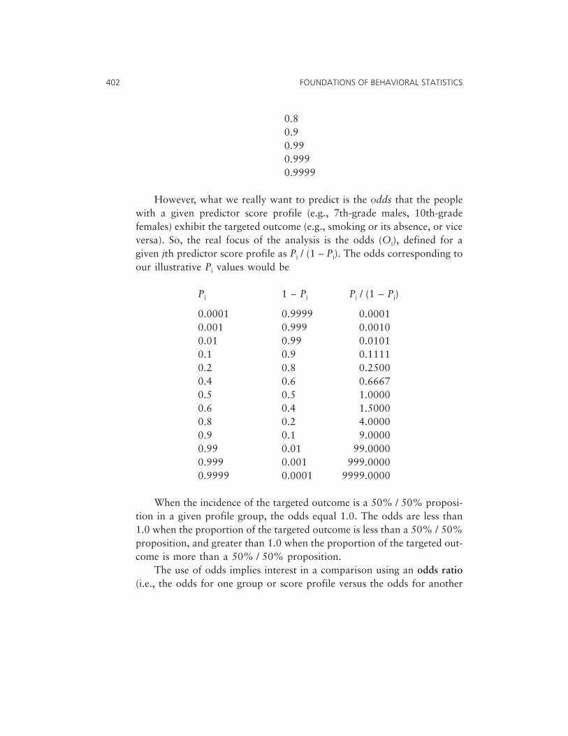
0.80.90.990.9990.9999

However, what we really want to predict is the odds that the peoplewith a given predictor score profile (e.g., 7th-grade males, 10th-gradefemales) exhibit the targeted outcome (e.g., smoking or its absence, or viceversa). So, the real focus of the analysis is the odds (Oj), defined for agiven jth predictor score profile as Pj / (1 – Pj). The odds corresponding toour illustrative Pj values would be

Pj 1 – Pj Pj / (1 – Pj)

0.0001 0.9999 0.00010.001 0.999 0.00100.01 0.99 0.01010.1 0.9 0.11110.2 0.8 0.25000.4 0.6 0.66670.5 0.5 1.00000.6 0.4 1.50000.8 0.2 4.00000.9 0.1 9.00000.99 0.01 99.00000.999 0.001 999.00000.9999 0.0001 9999.0000

When the incidence of the targeted outcome is a 50% / 50% proposi-tion in a given profile group, the odds equal 1.0. The odds are less than1.0 when the proportion of the targeted outcome is less than a 50% / 50%proposition, and greater than 1.0 when the proportion of the targeted out-come is more than a 50% / 50% proposition.

The use of odds implies interest in a comparison using an odds ratio(i.e., the odds for one group or score profile versus the odds for another


group or score profile). Here we are interested in the odds ratio forfemales versus males, or the odds ratio for less-educated versus more-edu-cated people. And in our Table 5.8 aspirin and heart attack example, the Pof a heart attack for physicians taking aspirin daily was 0.010 (i.e., 5 / 500;O = 0.010 / 0.990 = 0.0101), while the P of a heart attack for the physi-cians not taking a daily aspirin was 0.018 (O = 0.018 / 0.982 = 0.0183).Although the odds of myocardial infarct were small in both treatment con-ditions, the odds ratio (0.0101 / 0.0183 = 0.552) was sufficiently differentfrom 1.0 that in the parallel real study the investigation was halted beforethe planned completion date, and today adult patients are routinelyencouraged to take aspirin daily to minimize the risk of heart attack.

Log Odds as Outcomes

Unfortunately, there is an additional difficulty. Notice that at the largervalues of Pj, the odds become huge! For example, as we move from Pj =0.8 to Pj = 0.9, the corresponding odds move from Oj = 4.0 to Oj = 9.0.And at Pj values of 0.99, 0.999, and 0.9999, we obtain odds of 99.0,999.0, and 9999.0, respectively.

Figure 13.1 makes clear the exact nature of the problem. The figurepresents odds for our values of Pj ranging from 0.001 to 0.999. The sta-tistical difficulty of using the odds as the dependent variable in a classi-cal regression analysis is that odds are not linear. This would be less of


FIGURE 13.1. Plot of odds and corresponding logits

a difficulty if our data included Pj values that were less extreme, suchthat our odds did not reach hugely inflated values. However, we will usea transformation of the dichotomous outcome variable that will makelogistic regression reasonable whether or not our data include extraordi-nary odds.

Classical regression requires the form of the relationship between thepredictors and the outcome variable to be linear. When the relationship isnot linear, sometimes we can transform the independent variables tomodel curvilinear relationship, by adding predictor variables that take pre-dictors to various exponential powers, as illustrated in Chapter 9. In asimilar vein, here we will invoke a mathematical transformation of theoutcome variable (i.e., Oj) so that we can model nonlinear data dynamicswithin a linear model.

In conventional mathematics, we perform operations that count usingan additive function in the base unit of 1.0. An alternative is countinginstead with a multiplicative function using the base unit of 10, or 2.718,or any other number we wish to use as a base. Logarithms measure thepower to which the base must be raised to obtain a given value on X.

Our visit to logarithm land will be relatively brief. However, thereader is advised that the first experience of logarithms may be facili-tated by the presence of a dry gin martini, up, with a twist (Noolives!!!).

Common logarithms, by definition, use a base of 10. So consider thesedata for X that increase in multiples of 10: {10, 100, 1,000, 10,000}. Forthese data, we now have

X Base Exponent BaseEXPONENT

10 10 1 101

100 10 2 102

1,000 10 3 103

10,000 10 4 104

This means that, if we wish, we may reexpress our X scores in commonlog units as the value of the exponents:


X log X

10 1100 2

1,000 310,000 4

One feature of this reexpression is that the focus is shifted from abso-lute change to relative change. For example, if the X scores were dollars,the increases in worth are $90, $900, and $9,000, respectively. However,each increase reflects relative worth that grows by 10 times, or by1,000%. A model that focuses on relative increments of income might beof interest, for example, if we felt that absolute increases in income in dol-lars are insensitive to those people who value fixed absolute increases lessand less as they become more wealthy.

We measure the yield of hydrogen bombs in absolute or additiveterms, in megatons. A 1-megaton bomb releases the energy equivalent to 1million tons of TNT. A 2-megaton bomb releases an additional equivalentof another 1 million tons of TNT.

But we measure earthquakes using a common logarithmic (i.e., base10) scale. On the Richter scale, an increase of 1 magnitude unit representsa multiplicative factor of a relative increase of 10 times in the seismic waveamplitude. The seismic waves of a magnitude-7 earthquake are 10 timesgreater in amplitude than those of a magnitude-6 earthquake, 100 timeslarger than a magnitude-5 earthquake, and 1,000 times as large as a4-magnitude earthquake.

Logarithms are mathematically defined (i.e., can be computed) onlyfor values of X above zero. Oj is always greater than zero, because profilegroups with no incidence of the target outcome have no information avail-able to help us understand the likelihood of the outcome, and thus areexcluded. Logs are negative for values of X between 0 and 1. The log is 0when X = 1, because any number raised to the power of 0 equals 1.Finally, the log is a positive number for any X greater than 1.

Natural logs, unlike common logs, count instead in multiples of a basethat roughly equals 2.718. Logistic regression uses natural logs of the oddsas the focus of the analysis. Consider the following five scores on X


expressed in natural logs. These five scores reflect a constant relative,multiplicative increase of 171.83%:

Relative NaturalX % change Base Exponent Baseexp log X

1.00000 — 2.718282 0 1.0000 0.00002.71828 171.828 2.718282 1 2.7183 1.00007.38906 171.828 2.718282 2 7.3891 2.0000

20.08554 171.828 2.718282 3 20.0855 3.000054.59816 171.828 2.718282 4 54.5982 4.0000

148.41320 171.828 2.718282 5 148.4132 5.0000

Natural log values can be easily computed in Excel using the LN sta-tistical function. For example, if you type in

+LN(2.718282)

the program will return the value of 1.000. Conversely, if you type in

+EXP(1)

the program will return the value of 2.718282.The natural logs of values of odds are called logits. For selected values

of Pj and Oj, the logits (i.e., the rightmost column) are

LogPj 1 – Pj Pj / (1 – Pj) Pj / (1 – Pj)

0.0001 0.9999 0.0001 –9.2100.001 0.999 0.0010 –6.9070.01 0.99 0.0101 –4.5950.1 0.9 0.1111 –2.1970.2 0.8 0.2500 –1.3860.4 0.6 0.6667 –0.4050.5 0.5 1.0000 0.0000.6 0.4 1.5000 0.4050.8 0.2 4.0000 1.3860.9 0.1 9.0000 2.197


0.99 0.01 99.0000 4.5950.999 0.001 999.0000 6.9070.9999 0.0001 9999.0000 9.210

Table 13.1 presents the odds and logits for the smoking data, com-puted to help build a conceptual bridge between analyzing the dichoto-mous dummy-coded binary outcome data, using conventional regression,and doing the actual computations in logistic regression in a differentmanner. And Figure 13.1 illustrates that the logits form a linear pattern,even when odds have an extremely curvilinear pattern.

We can then run a classical regression to predict the Table 13.1 logitscores using education level and gender (dummy-coded as 0 = male and1 = female) as independent variables. The R2 is now 22.7%, versus ourprevious value of 5.9%, reflecting improved model fit when logits are theanalytic focus. Our a, b1, and b2 weights are 0.46, –0.05, and –0.73,respectively, or –0.046, 0.05, and 0.73, depending on whether we want topredict smoking or nonsmoking as the target outcome. In either case, theuncorrected effect size is R2 because, as we have previously learned, multi-plicative constants applied to Y (i.e., –1) do not affect squared correla-tions. However, there is another complication.

Estimation Theory

All the statistical methods taught in this book to this point invoke astatistical estimation theory called ordinary least squares (OLS). As wehave noted repeatedly, OLS estimation seeks weights that maximizeSOSEXPLAINED, minimize SOSERROR, and thus maximize uncorrected effectsizes analogous to r2.

The OLS estimates turn on the critical premise that sample data arerepresentative of population scores, and therefore do not take samplingerror into account. This works reasonably well when sampling error isminimal (e.g., sample size is quite large).

However, various other statistical estimation theories also can beused! Just as cursive writing is not mentioned to primary school studentsfirst learning to print, lest they form mass suicide pacts, some intellectualwithholding until now may have been justified to protect at least partiallythe reader’s mental health.


Maximum likelihood (ML) estimation theory differs from OLS meth-ods by focusing directly on estimating population parameters such as bweights (and not sample statistics). The OLS estimates will equal ML esti-mates when OLS analyses fully meet analytic assumptions. And OLSmethods have the advantage that they are computationally hugely moresimple. This advantage was critical in the days before the advent of mod-ern computers and software, when all analyses were repeatedly performedby hand to confirm that computation errors had not been made.

However, various classical regression assumptions (e.g., homoscedas-ticity) are difficult, if not impossible, to meet in the context of a dichoto-mous outcome variable. Thus, logistic regression software uses maximumlikelihood estimation theory to obtain statistics.

Maximum likelihood estimation does not use formulas to computestatistics. Instead, in a logistic regression model for given statistics esti-mates the probability of each case being a 1 or a 0 on the outcome variableis computed. If the persons in the dataset are independent of each other, aswhen people are independently sampled and the scores of given cases donot constrain other people’s scores, these probabilities can be multipliedtimes each other across all the cases to compute a likelihood function sta-tistic for the dataset. The parameter estimates achieve maximum likeli-hood when this likelihood function for a given dataset is largest.

Conceptually, the computer guesses statistical estimates of theweights, and keeps tweaking them until the likelihood function stopschanging much with repeated tweaking. Thus, logistic regression invokesanother form of the iteration process first described in Chapter 7. If youask, the computer software will divulge how many iterations were per-formed and what the guesses were at each iteration.

Maximizing the likelihood function is equivalent to maximizing thelog of the likelihood function. For our data, the log likelihood functionstabilized after three iterations. The estimates at each iteration were

LogIteration likelihood a weight b Education b Gender

1 –87.369 0.10616 –0.04540 –0.614422 –87.025 0.27554 –0.06043 –0.762573 –87.023 0.29094 –0.06176 –0.77368


The analyst need not fully understand the magic of this process. How-ever, when conducting analyses that invoke iteration, it is important toconfirm that the iteration “converges” (i.e., stabilizes). There is no guaran-tee that for a given dataset an iterative process will converge. So, to avoid“infinite loops,” software has a default maximum number of iterationsthat is allowed. If the solution does not converge, override the default iter-ation limits by allowing more iterations. If you set this number ridicu-lously high, and the solution still will not converge, the likely culprit isinsufficient sample size.

Result Interpretation

The first interpretation question, as usual, is “Do I have anything?” As inclassical regression, we can evaluate some combination of (a) NHSSTresults, (b) effect sizes, and (c) result replicability.

First, we can look at the statistical significance of our results. We com-pute the log-likelihood ratio for a model containing no predictor variablesas a baseline against which to compare results for alternative models.

The baseline is a model containing only a constant. In classical regres-sion, a model with only the a weight, or when all the predictors are useless,sets the a weight equal to MY, so that all the �Y i scores equal MY. The analo-gous process in logistic regression uses only the knowledge of baseline groupmembership (e.g., 30% smokers; 70% nonsmokers) to make predictions.

The log likelihood for our data, using only a prediction equation addi-tive constant, equals [n1{ln(P1)} + n0{ln(1 – P1}]. The log likelihood can beconverted to a χ2 test statistic by multiplying the log likelihood by –2.

For our smoking data, there were 45 smokers (30%) and 105 non-smokers (70%) out of 150 participants. So the test statistic is computed as

–2[n1{ln(P1)} + n0{ln(1 – P1}]–2[45{ln(0.3)} + 105{ln(1 – 0.3)}]

–2[45{ln(0.3)} + 105{ln(0.7)}]–2[45{–1.204} + 105{–0.357}]

–2[–54.179 + –37.451]–2[–91.6296]χ2 = 183.259


In an analogous fashion, the χ2 is computed for the model using the twopredictors, and for our data is 174.046.

Smaller χ2 values reflect better model fit. We want small values for χ2

(and larger pCALCULATED values) for the models we prefer, so that we do notreject the null that the model fits the data. However, in analyses that pre-sume large sample sizes, these test statistics are primarily useful in quanti-fying the differential fits of alternative models, and not in evaluatingoverall model fit, for the reasons noted in Chapters 6 and 7 (i.e., largesamples tend to yield statistical significance even when effect sizes aresmall).

Test statistic χ2 values and their degrees of freedom are both additive.This means that we can use these χ2 values to compute the statistical sig-nificance of model fit using a constant and two predictors versus usingonly the constant. For our data, we have 183.259 – 174.046 = 9.213. Theestimation of each additional model parameter costs df = 1. So, the dfspent to obtain the 9.213 improvement (i.e., decrease) in the χ2 was 2. Ifwe enter into Excel

+CHIDIST(9.213,2)

the program will return the pCALCULATED value of 0.010. Thus, using our twopredictor variables results in a statistically significant improvement overthe baseline model that uses only an additive constant.

Second, we can look at various effect sizes for our results. In classicalregression, the R2 can be computed as the ratio of the SOSMODEL to theSOSY. In logistic regression, there is the difficulty that “the model predictsthe logged odds, a transformation which represents a dependent variablewithout bounds and with an arbitrarily defined variance” (Pampel, 2000,p. 32) and thus a nonfixed and arbitrary SOS. However, a variety ofpseudo-R2 statistics has been suggested.

SPSS provides an estimate (RC&S2) suggested by Cox and Snell (1989).

For our data this estimate is 6.0%. However, Nagelkerke (1991) notedthat RC&S

2 cannot mathematically attain a limit of 1.0 for most datasets,and proposed computing the pseudo-R2

MAX and dividing RC&S2 by this

R2MAX to estimate the corrected value, RC&S

2*. SPSS also presents this cor-rected value, and for our data RC&S

2* = 8.4%.


Another alternative is the proportional improvement in χ2, computed as

RPROPORTIONAL2 = (χNULL

2 – χMODEL2) / χNULL

2 (13.1)


(183.259 – 174.046) / 183.2599.213 / 183.259

RPROPORTIONAL2 = 5.03%

Aldrich and Nelson (1984) proposed an alternative computed as

RA&S2 = (χNULL

2 – χMODEL2) / [(χNULL

2 – χMODEL2 + n) (13.2)


(183.259 – 174.046) / (183.259 – 174.046 + 150)9.213 / (9.213 + 150)

9.213 / 159.213RA&S

2 = 5.79%

Hagle and Mitchell (1992) noted that RA&S2 is attenuated, depending on

the distribution of the binary outcome scores, and they presented tablesfor correcting RA&S

2 to obtain RA&S2* by taking into account the percentage

of cases in the modal group. For our data, the modal group is nonsmokers,with 70% of the cases in this group. The corresponding tabled correctionfactor is 1.82. So, for our data we have

5.79%(1.82)RA&S

2* = 10.53%

Finally, given Equation 8.16

RY with X1, X2, . . . , Xj = rY with Y (8.16)


and Equation 8.17,

RY with X1, X2, . . . , Xj2 = rY with Y

2 (8.17)

a parallel procedure must be reasonable in logistical regression. In logisticregression, predicted membership in the outcome group dummy-coded as1 (here smoking) can be computed as

P1 = exp(b0 + b1 × 1 + . . . + bp × p) / [1 + exp(b0 + b1 × 1 + . . . + bp × p)] (13.3)

This equation can be used in future samples to predict group membership,invoking whatever baseline for the cutscore probability (e.g., 50%) theresearcher deems reasonable. But in the context of the present discussion,Pampel (2000, p. 53) suggested saving the predicted probabilities in SPSSusing the SAVE subcommand within the LOGISTIC REGRESSION procedure,and then using the CORRELATIONS procedure to correlate these probabili-ties with the observed outcome variable scores. For our data, this Pearsonr equals 0.2552, so the estimated R2 = 0.25522 = 6.5%.

Caution must be exercised when evaluating the logistic regressioneffect sizes. As Hosmer and Lemeshow (2000) noted, “Unfortunately lowR2 values in logistic regression are the norm and this presents a problemwhen reporting their values to an audience accustomed to seeing [classical]linear regression values” (p. 167).

Third, we can evaluate model invariance by replicating results with anindependent sample, or invoking cross-validation, or any of the previouslydescribed external and internal replicability analytic strategies. These anal-yses may be more feasible in logistic regression. In classical regression,researchers often seek a minimum sample size greater than the number ofmeasured variables times 10 (or 15 or 20). However, in logistic regression,researchers may require a sample size in the lower incidence outcomegroup (here nSMOKERS < nNONSMOKERS, nSMOKERS = 45) that is at least 10 timesthe number of predictor variables (Hosmer & Lemeshow, 2000). Thus,researchers may have larger sample sizes when invoking logistic regressionanalyses.

Several results may be consulted to answer the question “If I havesomething, from where does my noteworthy effect originate?” First, theequation weights may be examined. However, as output in conventional


software, these are not standardized weights, and so cannot be comparedwith each other apples-to-apples. One solution is to obtain semistandard-ized weights by standardizing only the predictor variables before runningthe logistic regression analysis (Pampel, 2000, pp. 32–33).

Second, structure coefficients may be computed in logistic regression.In the context of estimating R2 by squaring the correlation of predictedprobabilities with the dichotomous outcome variable (e.g., for our data,R2 = 0.25522 = 6.5%), we could analogously compute rS by correlating thepredictor variables with the predicted probabilities. For our data, thesestructure coefficients are –0.7496 and –0.8517, respectively.

�� Loglinear Analysis

As noted in the previous discussion of logistic regression, sometimes out-come variables are dichotomous. However, sometimes all the variables inan analysis are categorical. Loglinear analyses are powerful methods formodeling dynamics within categorical data. However, before presentingloglinear analysis, an historical precursor for loglinear analysis will first bepresented. This presentation will allow the comparative advantages ofloglinear analyses to be emphasized.

Pearson Contingency Table 2

Halpin et al. (1982) presented real data in The Journal of the AmericanMedical Association on Reye’s syndrome. The syndrome is a rare but quiteserious illness that usually occurs following influenza or chicken pox. Theresearchers were interested in exploring linkages between the syndromeand taking aspirin to treat these illnesses. Janet Rice (1992), a collaboratorin the research, used a related example in her thoughtful exposition ofloglinear analyses. Table 13.3 presents a related hypothetical dataset mod-eled on this research. Our example presumes that the data came from ret-rospective searches of clinical records, rather than from a randomizedclinical trial.

The classical Pearson χ2 test evaluates whether the proportional dis-tribution of cases within the contingency table is random (i.e., the cases



Variable

CaseReye’s

Syndrome Aspirin Gender

1 1 1 02 1 1 03 1 1 04 1 1 05 1 1 06 1 1 07 1 1 08 1 1 09 1 1 0

10 1 1 011 1 1 012 1 1 013 1 1 014 1 1 015 1 1 016 1 1 017 1 1 018 1 1 019 1 1 020 1 1 021 1 1 022 1 1 023 1 1 024 1 1 025 1 1 126 1 1 127 1 1 128 1 1 129 1 1 130 1 1 131 1 1 132 1 1 133 1 1 134 1 1 135 1 1 136 1 1 137 1 1 138 1 1 139 1 1 140 1 1 141 1 1 142 1 1 143 1 1 144 1 1 145 1 1 146 1 1 147 1 1 148 1 1 149 1 0 050 1 0 151 0 1 0

TABLE 13.3. Hypothetical Reye’s Syndrome Data


Variable

CaseReye’s

Syndrome Aspirin Gender

52 0 1 053 0 1 054 0 1 055 0 1 056 0 1 057 0 1 058 0 1 059 0 1 060 0 1 061 0 1 062 0 1 063 0 1 064 0 1 065 0 1 066 0 1 067 0 1 068 0 1 069 0 1 070 0 1 071 0 1 072 0 1 073 0 1 074 0 1 075 0 1 176 0 1 177 0 1 178 0 1 179 0 1 180 0 1 181 0 1 182 0 1 183 0 1 184 0 1 185 0 1 186 0 1 187 0 0 088 0 0 089 0 0 090 0 0 091 0 0 092 0 0 093 0 0 094 0 0 095 0 0 096 0 0 197 0 0 198 0 0 199 0 0 1100 0 0 1

TABLE 13.3. (cont.)

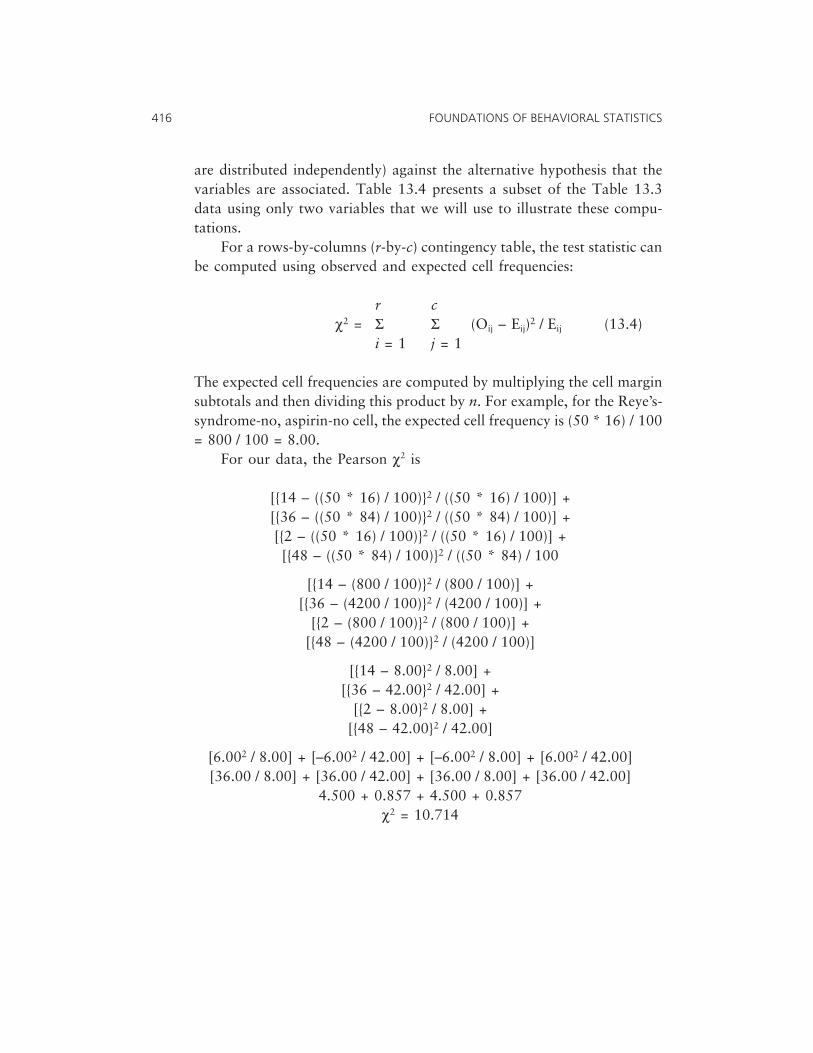
are distributed independently) against the alternative hypothesis that thevariables are associated. Table 13.4 presents a subset of the Table 13.3data using only two variables that we will use to illustrate these compu-tations.

For a rows-by-columns (r-by-c) contingency table, the test statistic canbe computed using observed and expected cell frequencies:

r cχ2 = Σ Σ (Oij – Eij)2 / Eij (13.4)

i = 1 j = 1

The expected cell frequencies are computed by multiplying the cell marginsubtotals and then dividing this product by n. For example, for the Reye’s-syndrome-no, aspirin-no cell, the expected cell frequency is (50 * 16) / 100= 800 / 100 = 8.00.

For our data, the Pearson χ2 is

[{14 – ((50 * 16) / 100)}2 / ((50 * 16) / 100)] +[{36 – ((50 * 84) / 100)}2 / ((50 * 84) / 100)] +[{2 – ((50 * 16) / 100)}2 / ((50 * 16) / 100)] +[{48 – ((50 * 84) / 100)}2 / ((50 * 84) / 100

[{14 – (800 / 100)}2 / (800 / 100)] +[{36 – (4200 / 100)}2 / (4200 / 100)] +

[{2 – (800 / 100)}2 / (800 / 100)] +[{48 – (4200 / 100)}2 / (4200 / 100)]

[{14 – 8.00}2 / 8.00] +[{36 – 42.00}2 / 42.00] +

[{2 – 8.00}2 / 8.00] +[{48 – 42.00}2 / 42.00]

[6.002 / 8.00] + [–6.002 / 42.00] + [–6.002 / 8.00] + [6.002 / 42.00][36.00 / 8.00] + [36.00 / 42.00] + [36.00 / 8.00] + [36.00 / 42.00]

4.500 + 0.857 + 4.500 + 0.857χ2 = 10.714


The Pearson contingency table χ2 test statistic has degrees of freedomequal to (rows minus 1) times (columns minus 1), which for our dataequal (2 – 1)(2 – 1), or 1. The pCALCULATED for this test (i.e., χ2 = 10.714; df =1) for our data is 0.00106. So we reject the null hypothesis that there is norelationship between the two variables reflected in the Table 13.4 cellcounts or proportions.

Now, what does this widely used statistic tell us? This crude resultsuggests that Reye’s syndrome, or aspirin, or the relationship of these twovariables, or some combination of these produces a nonzero association.But the specific origins of the effect are not elucidated by the Pearson χ2

analysis as it is classically conducted. As Ramsey and Schafer (1997) notedso succinctly, “Although the [Pearson contingency table] chi-squared testis one of the most widely used of statistical tools, it is also one of the leastinformative” (p. 548; emphasis added).

Logistic Alternative

In classical ANOVA, we could conduct a multiway study, pool together allthe explained sums of squares and their degrees of freedom, and then testa single, superomnibus null hypothesis of no difference among all the vari-ous main effect and cell means. For example, in a 4 × 3 factorial design,we could crudely lump together SOSA plus SOSB plus SOSA × B and then testthis superordinate SOSEXPLAINED with degrees of freedom equal to cells – 1(i.e., [4 × 3] – 1 = 11 = dfA = 3 + dfB = 2 + dfA × B = 6). However, testing ofsuch superomnibus ANOVA hypotheses in a multiway study makes no


TABLE 13.4. Contingency Table Layout of the Table13.3 Data for Reye’s Syndrome and Aspirin Variables

Aspirin

Reye’s Syndrome No Yes Total

No 14 36 50Yes 2 48 50Total 16 84 100

sense! We want to know where differences or relationships do or do notoccur.

In exactly the same vein, when analyzing multiway contingency tabledata, we also want to test separately the effects of the variables acting sin-gly and in various combinations with each other. Loglinear analysis hasthe compelling appeal that for a given design all possible models can betested. Thus, loglinear models have the capacity to help researchers isolatethe origins of detected relationships.

Loglinear analyses invoke the likelihood ratio χ2 test statistic, L2. Fora two-dimensional r-by-c contingency table,

r cL2 = Σ Σ 2[Oij][ln(Oij / Eij)] (13.5)

i = 1 j = 1

Equation 13.5 makes explicit that a logistic function is being invoked.For the Table 13.4 data we have

2(14)[ln(14 / 8.00)] + 2(36)[ln(36 / 42.00)]+ 2(2)[ln(2 / 8.00)] + 2(48)[ln(48 / 42.00)]

2(14)[ln(1.750)] + 2(36)[ln(0.857)]+ 2(2)[ln(0.250)] + 2(48)[ln(1.142)]

2(14)[0.560] + 2(36)[–0.154] + 2(2)[–1.386] + 2(48)[0.133]2(7.835) + 2(–5.549) + 2(–2.772) + 2(6.409)

15.669 + –11.098 + –5.545 + 12.818L2 = 11.844

The L2 is distributed as a χ2 and again has (r – 1)(c – 1) degrees of free-dom, or for our data, df = 1. The pCALCULATED for this test for our data is0.00058. Note that this pCALCULATED does not equal the pCALCULATED from thePearson χ2 for the same data (i.e., 0.00106).

The L2 and the Pearson χ2 will approach each other for the same dataas the sample size is larger. Nevertheless, the L2 test statistic is preferred inloglinear analyses. Unlike the Pearson χ2, the L2 test statistic has the criti-cal feature that for two nested models in which one model contains a sub-set of the terms in the other model, the model with the subset of terms willalways have a larger L2 test statistic than the other model. This critical fea-


ture allows the quantification of differential fits of alternative models, andstatistical significance testing of differential fit, which is precisely whatloglinear analysis is all about.

In addition to the commonality that logistic regression and loglinearanalyses both invoke natural logarithms, some loglinear analyses, likelogistic regression, also require iteration and maximum likelihood estima-tion of the expected values used in computing the likelihood function. Formore detailed comparisons of loglinear analysis and logistic regression, seeRice (1994).

Figure 13.2 presents the SPSS syntax used to perform all possiblemodel tests for our data. Table 13.5 presents the test statistics for each ofthe 19 models.

Interpretation Issues

When we are testing the fit of loglinear models to data, the null hypothesisis that the data are compatible with a given model. So we are seeking mod-els that are not statistically significant.

One complication is that more complex models have fewer degrees offreedom, and so become less and less falsifiable. And models with differentdegrees of freedom are difficult to compare apples-to-apples. One alterna-tive is to compute L2 / df as another comparative interpretation aid.

Finally, when a subset of alternative models fits reasonably well,among these we will tend to prefer simpler models. This is in keeping withthe admonitions of William of Occam, a sultan who, centuries ago, arguedthat when two explanations fit a set of facts, the more parsimoniousexplanation is more likely to be true. We prefer more parsimonious mod-els, because true findings are most likely to replicate.

When a particular variable is of interest, we can also conduct furthercomputations using the Table 13.5 test statistics to better understand thedynamics within our data. For example, presume that we are interested inexploring correlates of Reye’s syndrome. We test given relationships bycomputing χ2 difference test between models containing the effect of inter-est and models containing all the terms except the effect of interest. Thus,Table 13.6 tests the effect of the association for ill people between Reye’sand taking aspirin.


The effect due to the relationship of Reye’s and taking aspirin is statis-tically significant (L2 / χ2 = 11.8442, df = 1, pCALCULATED = 0.00058). Ofcourse, a definitive causal conclusion cannot be reached on the basis ofthese nonexperimental data, as emphasized in Chapter 1. Nevertheless, theresult is suggestive.


FIGURE 13.2. SPSS syntax for all possible loglinear models


TABLE 13.5. Model Fit Statistics for All 19 Possible Loglinear Models

Statistic

Model family/model pCALCULATED L2 df L2 / df

BaselineNull, equiprobability model 1.E-12 67.7762 7 9.682

Single MarginsReye’s 1.E-12 67.7762 6 11.296Aspirin 0.009 17.0807 6 2.847Gender 4.E-12 65.2052 6 10.868

Two MarginsReye’s, Aspirin 0.004 17.0807 5 3.416Reye’s, Gender 1.E-12 65.2052 5 13.041Aspirin, Gender 0.013 14.5097 5 2.902

Three MarginsReye’s, Aspirin, Gender 0.006 14.5097 4 3.627

Relationship Between Two VariablesReye’s, Aspirin, Reye’s by Aspirin 0.264 5.2365 4 1.309Reye’s, Gender, Reye’s by Gender 8.E-12 62.5650 4 15.641Aspirin, Gender, Aspirin by Gender 0.006 14.3499 4 3.587

Relationship and One Omitted MarginGender, Reye’s, Aspirin, Reye’s By Aspirin 0.446 2.6655 3 0.888Aspirin, Reye’s, Gender, Reye’s By Gender 0.008 11.8696 3 3.957Reye’s, Aspirin, Gender, Aspirin By Gender 0.002 14.3499 3 4.783

Two Relationships Among PredictorsReye’s, Aspirin, Gender, Reye’s By Aspirin, Reye’s ByGender

0.987 0.0253 2 0.013

Reye’s, Aspirin, Gender, Reye’s By Aspirin, Aspirin ByGender

0.286 2.5057 2 1.253

Reye’s, Aspirin, Gender, Reye’s By Gender, Aspirin ByGender

0.003 11.7098 2 5.855

Three Sets of RelationshipsReye’s, Aspirin, Gender, Reye’s By Aspirin, Reye’s ByGender, Aspirin By Gender

0.947 0.0044 1 0.004

Saturated (df = 0) ModelReye’s, Aspirin, Gender, Reye’s By Aspirin, Reye’s ByGender, Aspirin By Gender, Reye’s By Aspirin ByGender

1.000 0.0000 0 —

Note. The saturated model, which uses all possible table margins and relationships, like any model with zerodegrees of freedom, always fits the data perfectly, and thus is not falsifiable.

We can also test the main and interaction effects on an outcome ofinterest. Again, we test given effects by computing the χ2 difference testbetween models containing the effect of interest and models containing allthe terms except the effect of interest. Thus, Table 13.7 tests (a) the maineffect of aspirin on Reye’s for participants with either influenza or chicken


TABLE 13.6. Test of the Effect of the Reye’s By Aspirin Relationship Alone

Statistic

Model/effect χ2 (L2) df pCALCULATED

Reye’s, Aspirin, Gender, Aspirin By Gender 14.3499 3

Reye’s, Aspirin, Gender, REYE’S BY ASPIRIN, AspirinBy Gender

2.5057 2

Due to Reye’s By Aspirin Relationship 11.8442 1 0.00058

Note. The effect of the Reye’s By Aspirin relationship is evaluated by computing the differences in theχ2 / L2 values for the nested models, and then the pCALCULATED value for this L2 difference. ThepCALCULATED can be found using the Excel CHIDIST statistical function.

TABLE 13.7. Tests of the Effects of Aspirin and Gender,Controlling for Each Other

Statistic

Model/effect χ2 (L2) df pCALCULATED

Reye’s, Aspirin, Gender, Reye’s By Gender, Aspirin ByGender

11.7098 2

Reye’s, Aspirin, Gender, REYE’S BY ASPIRIN, Reye’sBy Gender, Aspirin By Gender

0.0044 1

Aspirin main effect controlling for Gender 11.7054 1 0.00062

Reye’s, Aspirin, Gender, Reye’s By Aspirin, Aspirin ByGender

2.5057 2

Reye’s, Aspirin, Gender, Reye’s By Aspirin, REYE’SBY GENDER, Aspirin By Gender

0.0044 1

Gender main effect controlling for Aspirin 2.5013 1 0.11375

Note. The main effects on Reye’s syndrome are evaluated by computing the differences in the χ2 / L2

values for the nested models and then the pCALCULATED values for these L2 differences. The pCALCULATEDvalues can be found using the Excel CHIDIST statistical function.

pox, controlling for gender, and (b) the main effect of gender on Reye’s forparticipants with either influenza or chicken pox, controlling for aspirin.

The aspirin main effect is statistically significant (pCALCULATED =0.00062), whereas the gender main effect is not (pCALCULATED = 0.11375).Again, however, we recall that the aspirin regimen in the hypothetical datawas not randomly assigned in a clinical trial, so strong causal conclusionsmay not be drawn. For example, perhaps the families more aggressivelytreating illness-related fever with aspirin may have had different diets, ordiffered in their genotypes.

We test the aspirin by gender two-way interaction effect on Reye’ssyndrome by computing the L2 / χ2 difference between the model contain-ing all terms except the three-relationship term (L2 / χ2 = 0.0044, df = 1),and the saturated model containing all the possible terms (L2 / χ2 = 0.0,df = 0). This interaction effect (L2 / χ2 = 0.0044, df = 1) is not statisticallysignificant (pCALCULATED = 0.94711).

However, interaction effects must be interpreted cautiously inloglinear analyses, just as in ANOVA. In a balanced 3 × 5 ANOVA with10 people per cell (n = 3 × 5 × 10 = 150), for example, the A-way maineffect means are each based on an n of 50, the B-way main effect meansare each based on an n of 30, and the interaction effects involve 15 meanseach with an n of 10. We estimate more parameters for higher-order inter-actions, and we pay the price for doing so, by spending more degrees offreedom. Lower ns for interaction estimates, and the associated greaterexpenditure of degrees of freedom, reduce power against Type II error forhigher-order ANOVA interaction effects versus lower-order effects.Exactly the same dynamics occur within the loglinear context.

Thus, from a variety of perspectives, these hypothetical data (modeledon real data) tell the story that people sick with influenza or chicken poxpossibly should avoid taking aspirin. No medication, or an alternativemedication, may represent the more prudent course of treatment.

Some Key Concepts

Logarithms focus on relative, multiplicative score changes rather thanabsolute, additive changes. Logarithmic transformation may be sensi-ble for substantive reasons, as when we believe that increments toincome have meaning only in the context of previous baselines forgiven people. Logarithmic transformations can also be useful for


statistical reasons, when data dynamics involve nonlinear patterns.Thus, these transformations are used in both logistic regression andloglinear analyses. Logistic regression and loglinear analyses alsohave in common the use of iteration and maximum likelihood estima-tion.

Logistic regression is used with a dichotomous outcome and pre-dictors that are some combination of interval or categorical.Polytomous logistic regression methods useful with outcomes involv-ing three or more categories have also been developed, but are beyondthe scope of the present treatment.

Predictive discriminant analysis (PDA) is an alternative to logisticregression (Huberty, 1994). PDA is a multivariate method not cov-ered in the present treatment. However, it will be noted that severalMonte Carlo simulation studies have compared the two methods(e.g., Halperin, Blackwelder, & Verter, 1971; Hosmer, Hosmer, &Fisher, 1983). In Monte Carlo studies, researchers create known pop-ulations, and then examine the capacity of alternative analyses torecover known parameters. Efron (1975) found that PDA is more sta-tistically efficient iff the assumptions of PDA are met.


1. For the various effect sizes considered in Chapters 1–12 (e.g., Cohen’s d,

η2 , ω2 , r2, adjusted R2), what were the effect sizes if the sample statistics

exactly matched the expectations of the nil null hypothesis? The odds

ratio is also an effect size. However, for odds ratios, what will the odds

ratio be if the odds are exactly equal in two groups (e.g., odds of infarct

among people taking a daily aspirin versus among people not taking a

daily aspirin)?

2. Create a dataset by computing odds (Pj / (1 – Pj)) for Pj ranging from 0.2

to 0.8 inclusive, incrementing by values of 0.01. Compute the correspond-

ing log odds values for the odds. First, plot the odds and logit data pairs

in a scattergram. Second, compute the Pearson r between the two vari-

ables. What do these graphical and statistical analyses suggest about the

necessity to use the logarithmic transform when values of Pj are not

extreme?


3. Compute the Pearson contingency table χ2 test for the variable pairs A

and B, and then C and D. Note that for both contingency tables, the

omnibus test χ2 = 9.0, df = 4, pCALCULATED = 0.06, and φ = 0.50. Then use

the SPSS LOGLINEAR command to test various models for both variable

pairs, and compare the model fit results. What do these comparisons sug-

gest about the appropriateness for multiway contingency tables of using

the omnibus χ2 test as the only analysis?


SPSS variables

Case A B C D

1 1 1 1 1

2 1 1 1 1

3 1 1 1 1

4 1 1 1 1

5 1 1 1 1

6 1 1 1 2

7 1 1 1 2

8 1 2 1 3

9 1 2 1 3

10 1 2 1 3

11 1 2 1 3

12 1 3 1 3

13 2 1 2 1

14 2 1 2 1

15 2 1 2 2

16 2 1 2 2

17 2 2 2 2

18 2 2 2 2

19 2 2 2 2

20 2 2 2 2

21 2 3 2 2

22 2 3 2 2

23 2 3 2 3

24 2 3 2 3

25 3 1 3 1


26 3 2 3 1

27 3 2 3 1

28 3 2 3 1

29 3 2 3 1

30 3 3 3 2

31 3 3 3 2

32 3 3 3 3

33 3 3 3 3

34 3 3 3 3

35 3 3 3 3

36 3 3 3 3

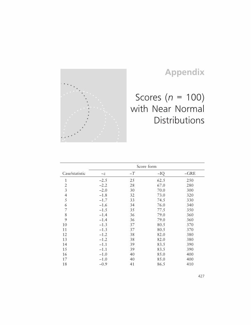
Appendix

Scores (n = 100)with Near Normal

Distributions

Score form

Case/statistic ~z ~T ~IQ ~GRE

1 –2.5 25 62.5 2502 –2.2 28 67.0 2803 –2.0 30 70.0 3004 –1.8 32 73.0 3205 –1.7 33 74.5 3306 –1.6 34 76.0 3407 –1.5 35 77.5 3508 –1.4 36 79.0 3609 –1.4 36 79.0 360

10 –1.3 37 80.5 37011 –1.3 37 80.5 37012 –1.2 38 82.0 38013 –1.2 38 82.0 38014 –1.1 39 83.5 39015 –1.1 39 83.5 39016 –1.0 40 85.0 40017 –1.0 40 85.0 40018 –0.9 41 86.5 410

427

19 –0.9 41 86.5 41020 –0.9 41 86.5 41021 –0.8 42 88.0 42022 –0.8 42 88.0 42023 –0.8 42 88.0 42024 –0.7 43 89.5 43025 –0.7 43 89.5 43026 –0.7 43 89.5 43027 –0.6 44 91.0 44028 –0.6 44 91.0 44029 –0.6 44 91.0 44030 –0.5 45 92.5 45031 –0.5 45 92.5 45032 –0.5 45 92.5 45033 –0.4 46 94.0 46034 –0.4 46 94.0 46035 –0.4 46 94.0 46036 –0.4 46 94.0 46037 –0.3 47 95.5 47038 –0.3 47 95.5 47039 –0.3 47 95.5 47040 –0.3 47 95.5 47041 –0.2 48 97.0 48042 –0.2 48 97.0 48043 –0.2 48 97.0 48044 –0.2 48 97.0 48045 –0.1 49 98.5 49046 –0.1 49 98.5 49047 –0.1 49 98.5 49048 –0.1 49 98.5 49049 0.0 50 100.0 50050 0.0 50 100.0 50051 0.0 50 100.0 50052 0.0 50 100.0 50053 0.1 51 101.5 51054 0.1 51 101.5 51055 0.1 51 101.5 51056 0.1 51 101.5 51057 0.2 52 103.0 52058 0.2 52 103.0 52059 0.2 52 103.0 52060 0.2 52 103.0 52061 0.3 53 104.5 53062 0.3 53 104.5 530

428 Appendix

63 0.3 53 104.5 53064 0.3 53 104.5 53065 0.4 54 106.0 54066 0.4 54 106.0 54067 0.4 54 106.0 54068 0.4 54 106.0 54069 0.5 55 107.5 55070 0.5 55 107.5 55071 0.5 55 107.5 55072 0.6 56 109.0 56073 0.6 56 109.0 56074 0.6 56 109.0 56075 0.7 57 110.5 57076 0.7 57 110.5 57077 0.7 57 110.5 57078 0.8 58 112.0 58079 0.8 58 112.0 58080 0.8 58 112.0 58081 0.9 59 113.5 59082 0.9 59 113.5 59083 0.9 59 113.5 59084 1.0 60 115.0 60085 1.0 60 115.0 60086 1.1 61 116.5 61087 1.1 61 116.5 61088 1.2 62 118.0 62089 1.2 62 118.0 62090 1.3 63 119.5 63091 1.3 63 119.5 63092 1.4 64 121.0 64093 1.4 64 121.0 64094 1.5 65 122.5 65095 1.6 66 124.0 66096 1.7 67 125.5 67097 1.8 68 127.0 68098 2.0 70 130.0 70099 2.2 72 133.0 720

100 2.5 75 137.5 750

M 0.000 50.000 100.000 500.000SD 1.005 10.048 15.073 100.483Skewness 0.000 0.000 0.000 0.000Kurtosis –0.170 –0.170 –0.170 –0.170

Appendix 429

References

Aaron, B., Kromrey, J. D., & Ferron, J. M. (1998, November). Equatingr-based and d-based effect size indices: Problems with a commonlyrecommended formula. Paper presented at the annual meeting of theFlorida Educational Research Association, Orlando, FL. (ERIC Docu-ment Reproduction Service No. ED 433 353)

Abelson, R. P. (1997). A retrospective on the significance test ban of 1999(If there were no significance tests, they would be invented). In L. L.Harlow, S. A. Mulaik, & J. H. Steiger (Eds.), What if there were nosignificance tests? (pp. 117–141). Mahwah, NJ: Erlbaum.

Aiken, L. S., & West, S. G. (1991). Multiple regression: Testing and inter-preting interactions. Newbury Park, CA: Sage.

Aldrich, J. H., & Nelson, F. D. (1984). Linear, probability, logit, andprobit models. Thousand Oaks, CA: Sage.

Algina, J., & Keselman, H. J. (2003). Approximate confidence intervalsfor effect sizes. Educational and Psychological Measurement, 63,537–553.

Algina, J., Keselman, H. J., & Penfield, R. D. (2005). Effect sizes and theirintervals: The two-level repeated measures case. Educational and Psy-chological Measurement, 65, 241–258.

Altman, D. G., Machin, D., Bryant, T. N., & Gardner, M. J. (2000). Sta-tistics with confidence: Confidence intervals and statistical guidelines(2nd ed.). London: British Medical Journal Books.

431

American Psychological Association. (2001). Publication manual of theAmerican Psychological Association (5th ed.). Washington, DC:Author.

Anderson, D. R., Burnham, K. P., & Thompson, W. (2000). Null hypoth-esis testing: Problems, prevalence, and an alternative. Journal ofWildlife Management, 64, 912–923.

Bagozzi, R. P., Fornell, C., & Larcker, D. F. (1981). Canonical correlationanalysis as a special case of a structural relations model. MultivariateBehavioral Research, 16, 437–454.

Baron, R. M., & Kenny, D. A. (1986). The moderator-mediator variabledistinction in social psychological research: Conceptual, strategic, andstatistical considerations. Journal of Personality and Social Psychol-ogy, 51, 1173–1182.

Beaton, A. E. (1973). Commonality. Princeton, NJ: Educational TestingService. (ERIC Document Reproduction Service No. ED 111 829)

Berkson, J. (1938). Some difficulties of interpretation encountered in theapplication of the chi-square test. Journal of the American StatisticalAssociation, 33, 526–536.

Berliner, D. C. (2002). Educational research: The hardest science of all.Educational Researcher, 31(8), 18–20.

Boik, R. J. (1979). Interactions, partial interactions, and interaction con-trasts in the analysis of variance. Psychological Bulletin, 86,1084–1089.

Boring, E. G. (1919). Mathematical vs. scientific importance. Psychologi-cal Bulletin, 16, 335–338.

Breaugh, J. A. (2003). Effect size estimation: Factors to consider and mis-takes to avoid. Journal of Management, 29, 79–97.

Campbell, D. T. (1957). Factors relevant to the validity of experiments insocial settings. Psychological Bulletin, 54, 297–312.

Campbell, D. T., & Erlebacher, A. (1975). How regression artifacts inquasi-experimental evaluations can mistakenly make compensatoryeducation look harmful. In M. Guttentag & E. L. Struening (Eds.),Handbook of evaluation research (Vol. 1, pp. 597–617). BeverlyHills: Sage.

Campbell, D. T., & Stanley, J. C. (1963). Experimental and quasi-experimental designs for research on teaching. In N. L. Gage (Ed.),Handbook of research on teaching (pp. 171–246). Chicago: RandMcNally.

Campbell, T. C. (2005). An introduction to clinical significance: An alter-native index of intervention effect for group experimental design.Journal of Early Intervention, 27, 210–227.

Capraro, R. M., & Capraro, M. (2002). Treatments of effect sizes and sta-tistical significance tests in textbooks. Educational and PsychologicalMeasurement, 62, 771–782.

432 References

Carr, S. C., & Thompson, B. (1996). The effects of prior knowledge andschema activation strategies on the inferential reading comprehensionof learning disabled and nonlearning disabled children. Learning Dis-abilities Quarterly, 19, 48–61.

Carter, D. S. (1979). Comparison of different shrinkage formulas in esti-mating population multiple correlation coefficients. Educational andPsychological Measurement, 39, 261–266.

Carver, R. (1978). The case against statistical significance testing. HarvardEducational Review, 48, 378–399.

Cattell, R. B. (1944). Psychological measurement: Normative, ipsative,interactive. Psychological Review, 51, 292–303.

Chambless, D. (1998). Defining empirically supported therapies. Journalof Consulting and Clinical Psychology, 66, 7–18.

Clark, H. H. (1973). The language-as-fixed-effect fallacy: A critique oflanguage statistics in psychological research. Journal of VerbalLearning and Verbal Behavior, 12, 335–359.

Cliff, N. (1987). Analyzing multivariate data. San Diego: Harcourt BraceJovanovich.

Cohen, J. (1968). Multiple regression as a general data-analytic system.Psychological Bulletin, 70, 426–443.

Cohen, J. (1969). Statistical power analysis for the behavioral sciences.New York: Academic Press.

Cohen, J. (1977). Statistical power analysis for the behavioral sciences(rev. ed.). Hillsdale, NJ: Erlbaum.

Cohen, J. (1988). Statistical power analysis for the behavioral sciences(2nd ed.). Hillsdale, NJ: Erlbaum.

Cohen, J. (1994). The earth is round (p < .05). American Psychologist, 49,997–1003.

Cohen, J., Cohen, P., West, S. G., & Aiken, L. S. (2003). Applied multipleregression/correlation analysis for the behavioral sciences (3rd ed.).Mahwah, NJ: Erlbaum.

Cooley, W. W., & Lohnes, P. R. (1971). Multivariate data analysis. NewYork: Wiley.

Courville, T., & Thompson, B. (2001). Use of structure coefficients inpublished multiple regression articles: β is not enough. Educationaland Psychological Measurement, 61, 229–248.

Cox, D. R. (1970). The analysis of binary data. London: Methuen.Cox, D. R., & Snell, E. J. (1989). Analysis of binary data (2nd ed.). Lon-

don: Chapman & Hall.Craeger, J. (1969). The interpretation of multiple regression via overlap-

ping rings. American Educational Research Journal, 6, 706–709.Cronbach, L. J. (1957). The two disciplines of scientific psychology.

American Psychologist, 12, 671–684.

References 433

Cronbach, L. J. (1975). Beyond the two disciplines of psychology. Ameri-can Psychologist, 30, 116–127.

Cumming, G., & Finch, S. (2001). A primer on the understanding, use andcalculation of confidence intervals that are based on central andnoncentral distributions. Educational and Psychological Measure-ment, 61, 532–575.

Cumming, G., & Finch, S. (2005). Inference by eye: Confidence intervals,and how to read pictures of data. American Psychologist, 60,170–180.

Dawson, T. E. (1999). Relating variance partitioning in measurementanalyses to the exact same process in substantive analyses. InB. Thompson (Ed.), Advances in social science methodology (Vol. 5,pp. 101–110). Stamford, CT: JAI Press.

Diaconis, P., & Efron, B. (1983). Computer-intensive methods in statis-tics. Scientific American, 248(5), 116–130.

Duncan, O. D. (1975). Introduction to structural equation models. NewYork: Academic Press.

Duncan, T. E., & Duncan, S. C. (1995). Modeling the process of develop-ment via latent growth curve methodology. Structural EquationModeling, 2, 187–213.

Duncan, T. E., Duncan, S. C., Strycker, L. A., Li, F., & Anthony, A.(1999). An introduction to latent variable growth curve modeling:Concepts, issues, and applications. Mahwah, NJ: Erlbaum.

Dunlap, W. P., & Landis, R. S. (1998). Interpretations of multiple regres-sion borrowed from factor analysis and canonical correlation. Jour-nal of General Psychology, 125, 397–407.

Edgington, E. S. (1974). A new tabulation of statistical procedures used inAPA journals. American Psychologist, 29, 25–26.

Edwards, A. E. (1985). Multiple regression and the analysis of varianceand covariance (2nd ed.). New York: Freeman.

Efron, B. (1975). The efficiency of logistic regression compared to normaldiscriminant analysis. Journal of the American Statistical Association,70, 892–898.

Efron, B. (1979). Bootstrap methods: Another look at the jackknife.Annals of Statistics, 7, 1–26.

Efron, B., & Tibshirani, R. J. (1993). An introduction to the bootstrap.New York: Chapman & Hall.

Elmore, P. B., & Woehlke, P. L. (1988). Statistical methods employed inAmerican Educational Research Journal, Educational Researcher,and Review of Educational Research from 1978 to 1987. EducationalResearcher, 17(9), 19–20.

Erlenmeyer-Kimling, L., & Jarvik, L. (1963). Genetics and intelligence: Areview. Science, 142, 1477–1479.

Ezekiel, M. (1930). Methods of correlational analysis. New York: Wiley.

434 References

Fan, X. (1996). Canonical correlation analysis as a general analytic model.In B. Thompson (Ed.), Advances in social science methodology (Vol.4, pp. 71–94). Greenwich, CT: JAI Press.

Fidler, F. (2002). The fifth edition of the APA Publication Manual: Whyits statistics recommendations are so controversial. Educational andPsychological Measurement, 62, 749–770.

Finch, S., Cumming, G., & Thomason, N. (2001). Reporting of statisticalinference in the Journal of Applied Psychology: Little evidence ofreform. Educational and Psychological Measurement, 61, 181–210.

Fisher, R. A. (1925). Statistical methods for research workers. Edinburgh:Oliver & Boyd.

Fisher, R. A. (1935). The design of experiments. Edinburgh: Oliver &Boyd.

Fowler, R. L. (1987). A general method for comparing effect magnitudesin ANOVA designs. Educational and Psychological Methods, 47,361–367.

Frazier, P. A., Tix, A.P., & Baron, K. E. (2004). Testing of moderator andmediator effects in counseling psychology research. Journal of Coun-seling Psychology, 51, 115–134.

Frederick, B. N. (1999). Fixed-, random-, and mixed-effects ANOVAmodels: A user-friendly guide for increasing the generalizability ofANOVA results. In B. Thompson, Advances in social science method-ology (Vol. 5, pp. 111–122). Stamford, CT: JAI Press.

Freedman, D. A. (1983). A note on screening regression equations. Ameri-can Statistician, 37, 152–155.

Friedman, H. (1968). Magnitude of experimental effect and a table for itsrapid estimation. Psychological Bulletin, 70, 245–251.

Gage, N. L. (1978). The scientific basis of the art of teaching. New York:Teachers College Press.

Galton, F. (1886). Regression towards mediocrity in hereditary stature.Journal of the Anthropological Institute, 15, 246–263.

Geisser, S., & Greenhouse, S. W. (1958). An extension of Box’s results onthe use of the F distribution in multivariate analysis. Annals of Math-ematical Statistics, 29, 885–891.

Girden, E. R. (1992). ANOVA: Repeated measures. Newbury Park, CA:Sage.

Glaser, K., Hojat, M., Veloski, J. J., Blacklow, R. S., & Goepp, C. E.(1992). Science, verbal, or qualitative skills: Which is the most impor-tant predictor of physician competence? Educational and Psychologi-cal Measurement, 52, 395–406.

Glass, G. V (1976). Primary, secondary, and meta-analysis of research.Educational Researcher, 5(10), 3–8.

Glass, G. V, McGaw, B., & Smith, M. L. (1981). Meta-analysis in socialresearch. Beverly Hills, CA: Sage.

References 435

Glass, G. V, & Stanley, J. C. (1970). Statistical methods in education andpsychology. Englewood Cliffs, NJ: Prentice-Hall.

Good, P. I., & Hardin, J. W. (2003). Common errors in statistics (andhow to avoid them). New York: Wiley.

Goodwin, L. D., & Goodwin, W. L. (1985). Statistical techniques in AERJarticles, 1979–1983: The preparation of graduate students to read theeducational research literature. Educational Researcher, 14(2), 5–11.

Gorsuch, R. L. (1983). Factor analysis (2nd ed.). Hillsdale, NJ: Erlbaum.Graham, J. M., Guthrie, A. C., & Thompson, B. (2003). Consequences of

not interpreting structure coefficients in published CFA research: Areminder. Structural Equation Modeling, 10, 142–153.

Greenwald, A. G. (1975). Consequences of prejudice against the nullhypothesis. Psychological Bulletin, 82, 1–20.

Grissom, R. J. (1994). Probability of the superior outcome of one treat-ment over another. Journal of Applied Psychology, 79, 314–316.

Grissom, R. J., & Kim, J. J. (2005). Effect sizes for research: A broadpractical approach. Mahwah, NJ: Erlbaum.

Guilford, J. (1954). Psychometric methods (2nd ed.). New York:McGraw-Hill.

Hagle, T. M., & Mitchell II, G. E. (1992). Goodness-of-fit measures forprobit and logit. American Journal of Political Science, 36, 762–784.

Halperin, W., Blackwelder, C., & Verter, J. (1971). Estimation ofmultivariate logistic risk function: A comparison of the discriminantfunction and maximum likelihood approaches. Journal of ChronicDiseases, 24, 125–158.

Halpin, T., Holtzhauer, F., Campbell, R., Hall, L., Correa-Villaseñor, A.,Lanese, R., Rice, J., & Hurwitz, E. (1982). Reye’s syndrome and druguse. Journal of the American Medical Association, 248, 687–691.

Harlow, L. L., Mulaik, S. A., & Steiger, J. H. (Eds.). (1997). What if therewere no significance tests?. Mahwah, NJ: Erlbaum.

Harris, K. (2003). Instructions for authors. Journal of Educational Psy-chology, 95, 201.

Harris, R. J. (1989). A canonical cautionary. Multivariate BehavioralResearch, 24, 17–39.

Harris, R. J. (1992, April). Structure coefficients versus scoring coeffi-cients as bases for interpreting emergent variables in multiple regres-sion and related techniques. Paper presented at the annual meeting ofthe American Educational Research Association, San Francisco.

Harwell, M. (1998). Misinterpreting interaction effects in analysis of vari-ance. Measurement and Evaluation in Counseling and Development,31, 125–136.

Hays, W. L. (1981). Statistics (3rd ed.). New York: Holt, Rinehart &Winston.

Hedges, L. V. (1981). Distribution theory for Glass’s estimator of effect

436 References

size and related estimators. Journal of Educational Statistics, 6,107–128.

Hedges, L. V., & Olkin, I. (1985). Statistical methods for meta-analysis.San Diego: Academic Press.

Henson, R. K. (1999). Multivariate normality: What is it and how is itassessed? In B. Thompson (Ed.), Advances in social science methodol-ogy (Vol. 5, pp. 193–212). Stamford, CT: JAI Press.

Herzberg, P. A. (1969). The parameters of cross-validation. Psycho-metrika Monograph Supplement, 16, 1–67.

Hess, B., Olejnik, S., & Huberty, C. J (2001). The efficacy of twoImprovement-over-chance effect sizes for two-group univariate com-parisons under variance heterogeneity and nonnormality. Educa-tional and Psychological Measurement, 61, 909–936.

Hester, Y. C. (2000). An analysis of the use and misuse of ANOVA. (Doc-toral dissertation, Texas A&M University.) Dissertation AbstractsInternational, 61, 4332A. (University Microfilms No. AAT9994257)

Hicks, C. R. (1973). Fundamental concepts in the design of experiments(2nd ed.). New York: Holt, Rinehart & Winston.

Hicks, L. (1970). Some properties of ipsative, normative, and forced-choice normative measures. Psychological Bulletin, 74, 167–184.

Horst, P. (1931). A proof that the point from which the sum of the abso-lute deviations is a minimum is the median. Journal of EducationalPsychology, 22(3), 25–26.

Horst, P. (1966). Psychological measurement and prediction. Belmont,CA: Wadsworth.

Hosmer, D. W., & Lemeshow, S. (2000). Applied logistic regression (2nded.). New York: Wiley.

Hosmer, T., Hosmer, D., & Fisher, L. (1983). A comparison of the maxi-mum likelihood and discriminant function estimators of the coeffi-cients of the logistic regression model for mixed continuous anddiscrete variables. Communications in Science, B12, 577–593.

Howell, D. C. (2002). Statistical methods for psychology (6th ed.). PacificGrove, CA: Duxbury.

Hubbard, R., & Ryan, P. A. (2000). The historical growth of statisticalsignificance testing in psychology—and its future prospects. Educa-tional and Psychological Measurement, 60, 661–681.

Huber, P. J. (1981). Robust statistics. New York: Wiley.Huberty, C. J (1989). Problems with stepwise methods—better alterna-

tives. In B. Thompson (Ed.), Advances in social science methodology(Vol. 1, pp. 43–70). Greenwich, CT: JAI Press.

Huberty, C. J (1994). Applied discriminant analysis. New York: Wiley.Huberty, C. J (1999). On some history regarding statistical testing. In

B. Thompson (Ed.), Advances in social science methodology (Vol. 5,pp. 1–23). Stamford, CT: JAI Press.

References 437

Huberty, C. J (2002). A history of effect size indices. Educational and Psy-chological Measurement, 62, 227–240.

Huberty, C. J, & Holmes, S. E. (1983). Two-group comparisons andunivariate classification. Educational and Psychological Measure-ment, 43, 15–26.

Huberty, C. J, & Lowman, L. L. (2000). Group overlap as a basis foreffect size. Educational and Psychological Measurement, 60,543–563.

Huberty, C. J, & Morris, J. D. (1988). A single contrast test procedure.Educational and Psychological Measurement, 48, 567–578.

Huck, S. W. (1992). Group heterogeneity and Pearson’s r. Educationaland Psychological Measurement, 52, 253–260.

Huck, S. W., Cormier, W. H., & Bounds, W. G., Jr. (1974). Reading sta-tistics and research. New York: Harper & Row.

Huck, S. W., Wright, S. P., & Park, S. (1992). Pearson’s r and spread: Aclassroom demonstration. Teaching of Psychology, 19(1), 45–47.

Huitema, B. E. (1980). The analysis of covariance and alternatives. NewYork: Wiley.

Humphreys, L. G. (1978). Doing research the hard way: Substituting anal-ysis of variance for a problem in correlational analysis. Journal ofEducational Psychology, 70, 873–876.

Humphreys, L. G., & Fleishman, A. (1974). Pseudo-orthogonal and otheranalysis of variance designs involving individual-differences variables.Journal of Educational Psychology, 66, 464–472.

Huynh, H., & Feldt, L. S. (1976). Estimation of the Box correction fordegrees of freedom from sample data in randomized block and split-plot designs. Journal of Educational Statistics, 1, 69–82.

International Committee of Medical Journal Editors. (1997). Uniformrequirements for manuscripts submitted to biomedical journals.Annals of Internal Medicine, 126, 36–47.

Johnson, H. G. (1985). Beneath the technological fix: Outliers and proba-bility statements. Journal of Chronic Diseases, 38, 957–961.

Jones, L. V. (1955). Statistics and research design. Annual Review of Psy-chology, 6, 405–430.

Kendall, P. C. (1999). Clinical significance. Journal of Consulting andClinical Psychology, 67, 283–284.

Kendall, P. C., Marrs-Garcia, A., Nath, S. R., & Sheldrick, R. C. (1999).Normative comparisons for the evaluation of clinical significance.Journal of Counseling and Consulting Psychology, 67, 285–299.

Kennedy, J. J., & Bush, A. J. (1985). An introduction to the design andanalysis of experiments in behavioral research. Lanham, MD: Univer-sity Press of America.

Keppel, G., & Zedeck, S. (1989). Data analysis for research designs. NewYork: Freeman.

438 References

Kerlinger, F. N. (1977). The influence of research on educational practice.Educational Researcher, 6(8), 5–12.

Kerlinger, F. N. (1986). Foundations of behavioral research (3rd ed.).New York: Holt, Rinehart & Winston.

Kerlinger, F. N., & Pedhazur, E. J. (1973). Multiple regression in behav-ioral research. New York: Holt, Rinehart & Winston.

Keselman, H. J., Huberty, C. J, Lix, L. M., Olejnik, S., Cribbie, R.,Donahue, B., Kowalchuk, R. K., Lowman, L. L., Petoskey, M. D.,Keselman, J. C., & Levin, J. R. (1998). Statistical practices of educa-tional researchers: An analysis of their ANOVA, MANOVA andANCOVA analyses. Review of Educational Research, 68, 350–386.

Keselman, H. J., Kowalchuk, R. K., & Lix, L. M. (1998). Robustnonorthogonal analyses revisited: An update based on trimmedmeans. Psychometrika, 63, 145–163.

Keselman, H. J., Lix, L. M., & Kowalchuk, R. K. (1998). Multiple com-parison procedures for trimmed means. Psychological Methods, 3,123–141.

Kieffer, K. M., Reese, R. J., & Thompson, B. (2001). Statistical techniquesemployed in AERJ and JCP articles from 1988 to 1997: A method-ological review. Journal of Experimental Education, 69, 280–309.

Kimbell, A. (2001, February). The basic concepts of the General LinearModel (GLM): Canonical correlation analysis (CCA) as a GLM.Paper presented at the annual meeting of the Southwest EducationalResearch Association, New Orleans. (ERIC Document ReproductionService No. ED 450 147)

Kirk, R. E. (Ed.). (1972). Statistical issues: A reader for the behavioral sci-ences. Monterey, CA: Brooks/Cole.

Kirk, R. E. (1996). Practical significance: A concept whose time has come.Educational and Psychological Measurement, 56, 746–759.

Kirk, R. E. (2003). The importance of effect magnitude. In S. F. Davis(Ed.), Handbook of research methods in experimental psychology(pp. 83–105). Oxford, UK: Blackwell.

Kline, R. (2004). Beyond significance testing: Reforming data analysismethods in behavioral research. Washington, DC: American Psycho-logical Association.

Knapp, T. R. (1978). Canonical correlation analysis: A general parametricsignificance testing system. Psychological Bulletin, 85, 410–416.

Knapp, T., & Sawilowsky, S. (2001). Constructive criticisms of method-ological and editorial practices. Journal of Experimental Education,70, 65–79.

Kulik, J., & Kulik, C-L. (1992). Meta-analysis: Historical origins and con-temporary practice. In B. Thompson (Ed.), Advances in social sciencemethodology (Vol. 2, pp. 53–80). Greenwich, CT: JAI Press.

Levene, H. (1960). Robust tests for equality of variances. In I. Olkin, S. G.

References 439

Ghurye, W. Hoeffding, W. G. Madow, & H. B. Mann (Eds.), Contri-butions to probability and statistics: Essays in honor of HaroldHotelling (pp. 278–292). Stanford, CA: Stanford University Press.

Levin, J. R., & Marascuilo, L. A. (1972). Type IV errors and interactions.Psychological Bulletin, 78, 368–374.

Levine, M. S. (1977). Canonical analysis and factor comparison. BeverlyHills, CA: Sage.

Likert, R. (1932). A technique for the measurement of attitudes. Archivesof Psychology, no. 32.

Little, R. J. A., & Rubin, D. R. (1987). Statistical analysis with missingdata. New York: Wiley.

Loehlin, J. C. (2004). Latent variable models: An introduction to factor,path, and structural equation analysis (4th ed.). Mahwah, NJ:Erlbaum.

Loftin, L., & Madison, S. (1991). The extreme dangers of covariance cor-rections. In B. Thompson (Ed.), Advances in educational research:Substantive findings, methodological developments (Vol. 1, pp.133–147). Greenwich, CT: JAI Press.

Love, G. (1988, November). Understanding experimentwise error proba-bility. Paper presented at the annual meeting of the Mid-South Educa-tional Research Association, Louisville, KY. (ERIC DocumentReproduction Service No. ED 304 451)

Lunneborg, C. E. (1999). Data analysis by resampling: Concepts andapplications. Pacific Grove, CA: Duxbury.

Lunneborg, C. E. (2001). Random assignment of available cases: Boot-strap standard errors and confidence intervals. PsychologicalMethods, 6, 402–412.

McCartney, K., & Rosenthal, R. (2000). Effect size, practical importance,and social policy for children. Child Development, 71, 173–180.

Mangel, M., & Samaniego, F. J. (1984). Abraham Wald’s work on air-craft survivability. Journal of the American Statistical Association,79, 259–267.

Marascuilo, L. A., & Levin, J. R. (1970). Appropriate post hoc compari-sons for interaction and nested hypotheses in analysis of variancedesigns: The elimination of Type IV errors. American EducationalResearch Journal, 7, 397–421.

Maxwell, S. E., & Delaney, H. D. (2004). Designing experiments and ana-lyzing data (2nd ed.). Mahwah, NJ: Erlbaum.

Menard, S. (2002). Applied logistic regression (2nd ed.). Thousand Oaks,CA: Sage.

Meredith, W. (1964). Canonical correlations with fallible data.Psychometrika, 29, 55–65.

Mittag, K. C., & Thompson, B. (2000). A national survey of AERA mem-

440 References

bers’ perceptions of statistical significance tests and other statisticalissues. Educational Researcher, 29(4), 14–20.

Mood, A. R. (1969). Macro-analysis of the American educational system.Operations Research, 17, 770–784.

Mosier, C. I. (1951). The need and means of cross-validation, I: Problemsand design of cross-validation. Educational and Psychological Mea-surement, 11, 5–11.

Mosteller, F., & Boruch, R. (Eds.). (2002). Evidence matters: Randomizedtrials in education research. Washington, DC: Brookings InstitutionPress.

Mulaik, S. A., Raju, N. S., & Harshman, R. A. (1997). There is a time andplace for significance testing. In L. L. Harlow, S. A. Mulaik, & J. H.Steiger (Eds.), What if there were no significance tests? (pp. 65–115).Mahwah, NJ: Erlbaum.

Nagelkerke, N. J. D. (1991). A note on a general definition of the coeffi-cient of determination. Biometrika, 78, 691–692.

Nelson, N., Rosenthal, R., & Rosnow, R. L. (1986). Interpretation of sig-nificance levels and effect sizes by psychological researchers. Ameri-can Psychologist, 41, 1299–1301.

Nunnally, J. C. (1975). Psychometric theory—25 years ago and now. Edu-cational Researcher, 4(10), 7–14, 19–20.

Nunnally, J. C. (1978). Psychometric methods (2nd ed.). New York:McGraw-Hill.

Oakes, M. (1986). Statistical inference: A commentary for the social andbehavioral sciences. New York: Wiley.

Odom, S. L., Brantlinger, E., Gersten, R., Horner, R. H., & Thompson, B.(2005). Research in special education: Scientific methods and evi-dence-based practices. Exceptional Children, 71, 137–148.

Olejnik, S., & Algina, J. (2000). Measures of effect size for comparativestudies: Applications, interpretations, and limitations. ContemporaryEducational Psychology, 25, 241–286.

Olejnik, S., & Algina, J. (2003). Generalized eta and omega squared statis-tics: Measures of effect size for some common research designs. Psy-chological Methods, 8, 434–437.

Ott, L. (1984). Introduction to statistical methods and data analysis.Boston: Prindle, Weber, & Schmidt.

Pampel, F. C. (2000). Logistic regression: A primer. Thousand Oaks, CA:Sage.

Pedhazur, E. J. (1977). Coding subjects in repeated measures designs. Psy-chological Bulletin, 34, 298–305.

Pedhazur, E. J. (1982). Multiple regression in behavioral research: Expla-nation and prediction (2nd ed.). New York: Holt, Rinehart &Winston.

References 441

Pedhazur, E. J., & Schmelkin, L. P. (1991). Measurement, design, andanalysis: An integrated approach. Hillsdale, NJ: Erlbaum.

Popper, K. R. (1961). The logic of scientific discovery. New York: ScienceEditions.

Popper, K. R. (1965). Conjectures and refutations (2nd ed.). New York:Harper Torchbooks.

Ramsey, F. L., & Schafer, D. W. (1997). The statistical sleuth: A course inmethods of data analysis. Belmont, CA: Duxbury.

Raudenbush, S. W. (2005). Learning from attempts to improve schooling:The contribution of methodological diversity. EducationalResearcher, 34(5), 25–31.

Rencher, A. C., & Pun, F-C. (1980). Inflation of R2 in best subset regres-sion. Technometrics, 22, 49–53.

Rice, J. (1992). Loglinear analysis: Analysis of categorical variables in thelogit setting. In B. Thompson (Ed.), Advances in social science meth-odology (Vol. 2, pp. 1–52). Greenwich, CT: JAI Press.

Rice, J. (1994). Logistic regression: An introduction. In B. Thompson(Ed.), Advances in social science methodology (Vol. 3, pp. 191–245).Greenwich, CT: JAI Press.

Robertson, C. (1991). Computationally intensive statistics. In P. Lovie &A. Lovie (Eds.), New developments in statistics for psychology andthe social sciences (Vol. 2, pp. 49–80). Leicester, UK: British Psycho-logical Society.

Robinson, D. H., & Wainer, H. (2002). On the past and future of nullhypothesis significance testing. Journal of Wildlife Management, 66,263–271.

Robinson, W. S. (1950). Ecological correlations and the behavior of indi-viduals. American Sociological Review, 15, 351–357.

Rokeach, M. (1973). The nature of human values. New York: Free Press.Ronis, D. L. (1981). Comparing the magnitude of effects in ANOVA

designs. Educational and Psychological Measurement, 41, 993–1000.Rosenthal, R. (1979). The “file drawer problem” and tolerance for null

results. Psychological Bulletin, 86, 638–641.Rosenthal, R. (1994). Parametric measures of effect size. In H. Cooper &

L. V. Hedges (Eds.), The handbook of research synthesis (pp.231–244). New York: Russell Sage Foundation.

Rosenthal, R., & Gaito, J. (1963). The interpretation of level of signifi-cance by psychological researchers. Journal of Psychology, 55,33–38.

Rosenthal, R., & Rubin, D. (1979). A note on percent variance explainedas a measure of the importance of effects. Journal of Applied SocialPsychology, 9, 395–396.

Rosnow, R. L., & Rosenthal, R. (1989a). Definition and interpretation ofinteraction effects. Psychological Bulletin, 105, 143–146.

442 References

Rosnow, R. L., & Rosenthal, R. (1989b). Statistical procedures and thejustification of knowledge in psychological science. American Psy-chologist, 44, 1276–1284.

Rosnow, R. L., & Rosenthal, R. (1991). If you’re looking at the cellmeans, you’re not looking at only the interaction (unless all maineffects are zero). Psychological Bulletin, 110, 574–576.

Rowell, R. K. (1996). Partitioning predicted variance into constituentparts: How to conduct commonality analysis. In B. Thompson (Ed.),Advances in social science methodology (Vol. 4, pp. 33–44). Green-wich, CT: JAI Press.

Rozeboom, W. W. (1997). Good science is abductive, not hypothetico-deductive. In L. L. Harlow, S. A. Mulaik, & J. H. Steiger (Eds.), Whatif there were no significance tests? (pp. 335–392). Mahwah, NJ:Erlbaum.

Rubin, D. B. (1974). Estimating causal effects of treatments in randomizedand nonrandomized studies. Journal of Educational Psychology, 66,688–701.

Sackett, D. L., Straus, S. E., Richardson, W. S., Rosenberg, W., & Haynes,R. B. (2000). Evidence-based medicine: How to practice and teachEBM (2nd ed.). New York: Churchill Livingstone.

Satterthwaite, F. W. (1946). An approximate distribution of estimates ofvariance components. Biometrics Bulletin, 2, 110–114.

Schmidt, F. L. (1996). Statistical significance testing and cumulativeknowledge in psychology: Implications for the training of researchers.Psychological Methods, 1, 115–129.

Schmidt, F. L., & Hunter, J. E. (1997). Eight common but false objectionsto the discontinuation of significance testing in the analysis ofresearch data. In L. L. Harlow, S. A. Mulaik, & J. H. Steiger (Eds.),What if there were no significance tests? (pp. 37–64). Mahwah, NJ:Erlbaum.

Schulzer, M., & Mancini, G. B. J. (1996). “Unqualified success” and“unmitigated” failure: Number needed-to-treat related concepts forassessing treatment efficacy in the presence of treatment inducedadverse effects. International Journal of Epidemiology, 25, 704–712.

Seibold, D. R., & McPhee, R. D. (1979). Commonality analysis: Amethod for decomposing explained variance in multiple regressionanalyses. Human Communication Research, 5, 355–365.

Shavelson, R. J., & Towne, L. (Eds.). (2002). Scientific research in educa-tion. Washington, DC: National Academy Press.

Shaver, J. (1985). Chance and nonsense. Phi Delta Kappan, 67(1), 57–60.Shrout, P. E., & Bolger, N. (2002). Mediation in experimental and non-

experimental studies: New procedures and recommendations. Psy-chological Methods, 7, 422–445.

References 443

Siegel, S. (1956). Nonparametric statistics for the behavioral sciences.New York: McGraw-Hill.

Simpson, C. (1951). The interpretation of interaction in contingencytables. Journal of the Royal Statistical Society, 13, 238–241.

Smithson, M. (2000). Statistics with confidence. London: Sage.Smithson, M. (2001). Correct confidence intervals for various regression

effect sizes and parameters: The importance of noncentral distribu-tions in computing intervals. Educational and Psychological Measure-ment, 61, 605–632.

Smithson, M. (2002). Confidence intervals. Thousand Oaks, CA: Sage.Snedecor, G. W. (1934). Calculation and interpretation of analysis of vari-

ance and covariance. Ames, IA: Collegiate Press.Snyder, P. (1991). Three reasons why stepwise regression methods should

not be used by researchers. In B. Thompson (Ed.), Advances in educa-tional research: Substantive findings, methodological developments(Vol. 1, pp. 99–105). Greenwich, CT: JAI Press.

Snyder, P. (2000). Guidelines for reporting results of group quantitativeinvestigations. Journal of Early Intervention, 23, 145–150.

Snyder, P., & Lawson, S. (1993). Evaluating results using corrected anduncorrected effect size estimates. Journal of Experimental Education,61, 334–349.

Steering Committee of the Physicians’ Health Study Research Group.(1988). Preliminary report: Findings from the aspirin component ofthe ongoing physicians’ health study. New England Journal of Medi-cine, 318, 262–264.

Steiger, J. H., & Fouladi, R. T. (1992). R2: A computer program for inter-val estimation, power calculation, and hypothesis testing for thesquared multiple correlation. Behavior Research Methods, Instru-ments, and Computers, 4, 581–582.

Stevens, J. (1996). Applied multivariate statistics for the social sciences(3rd ed.). Mahwah, NJ: Erlbaum.

Stevens, S. (1946). On the theory of scales of measurement. Science, 103,677–680.

Stevens, S. (1951). Mathematics, measurement, and psychophysics. InS. Stevens (Ed.), Handbook of experimental psychology (pp. 1–49).New York: Wiley.

Stevens, S. (1968). Measurement, statistics, and the schemapiric view. Sci-ence, 161, 849–856.

“Student.” [W. S. Gosset] (1908). The probable error of a mean.Biometrika, 6, 1–25.

Tanguma, J. (1999). Analyzing repeated measures designs using univariateand multivariate methods: A primer. In B. Thompson (Ed.), Advancesin social science methodology (Vol. 5, pp. 233–250). Stamford, CT:JAI Press.

444 References

Tashakkori, A., & Teddlie, C. (Eds.). (2002). Handbook of mixed meth-ods social and behavioral research. Thousand Oaks, CA: Sage.

Tatsuoka, M. M. (1975). The general linear model: A “new” trend inanalysis of variance (Selected topics in advanced statistics: An elemen-tary approach, no. 7). Champaign, IL: Institute for Personality andAbility Testing.

Thompson, B. (1985). Alternate methods for analyzing data from experi-ments. Journal of Experimental Education, 54, 50–55.

Thompson, B. (1986). ANOVA versus regression analysis of ATI designs:An empirical investigation. Educational and Psychological Measure-ment, 46, 917–928.

Thompson, B. (1988a). Discarding variance: A cardinal sin in research.Measurement and Evaluation in Counseling and Development, 21,3–4.

Thompson, B. (1988b). Program FACSTRAP: A program that computesbootstrap estimates of factor structure. Educational and Psychologi-cal Measurement, 48, 681–686.

Thompson, B. (1989a). Statistical significance, result importance, andresult generalizability: Three noteworthy but somewhat differentissues. Measurement and Evaluation in Counseling and Development,22, 2–6.

Thompson, B. (1989b). Why won’t stepwise methods die? Measurementand Evaluation in Counseling and Development, 21(4), 146–148.

Thompson, B. (1991a). A primer on the logic and use of canonical correla-tion analysis. Measurement and Evaluation in Counseling and Devel-opment, 24, 80–95.

Thompson, B. (1991b). Review of Data analysis for research designs.Educational and Psychological Measurement, 51, 500–510.

Thompson, B. (1992a). DISCSTRA: A computer program that computesbootstrap resampling estimates of descriptive discriminant analysisfunction and structure coefficients and group centroids. Educationaland Psychological Measurement, 52, 905–911.

Thompson, B. (1992b). Misuse of ANCOVA and related “statistical con-trol” procedures. Reading Psychology, 13(1), iii–xviii.

Thompson, B. (1992c). Two and one-half decades of leadership in mea-surement and evaluation. Journal of Counseling and Development,70, 434–438.

Thompson, B. (1993). The use of statistical significance tests in research:Bootstrap and other alternatives. Journal of Experimental Education,61, 361–377.

Thompson, B. (1994a). Guidelines for authors. Educational and Psycho-logical Measurement, 54, 837–847.

Thompson, B. (1994b). The pivotal role of replication in psychological

References 445

research: Empirically evaluating the replicability of sample results.Journal of Personality, 62, 157–176.

Thompson, B. (1994c). Planned versus unplanned and orthogonal versusnonorthogonal contrasts: The neo-classical perspective. In B. Thomp-son (Ed.), Advances in social science methodology (Vol. 3, pp. 3–27).Greenwich, CT: JAI Press.

Thompson, B. (1995). Stepwise regression and stepwise discriminant anal-ysis need not apply here: A guidelines editorial. Educational and Psy-chological Measurement, 55, 525–534.

Thompson, B. (1996). AERA editorial policies regarding statistical signifi-cance testing: Three suggested reforms. Educational Researcher,25(2), 26–30.

Thompson, B. (1999a). If statistical significance tests are broken/misused,what practices should supplement or replace them? Theory & Psy-chology, 9, 167–183.

Thompson, B. (1999b). Journal editorial policies regarding statistical sig-nificance tests: Heat is to fire as p is to importance. Educational Psy-chology Review, 11, 157–169.

Thompson, B. (2000a). Canonical correlation analysis. In L. Grimm & P.Yarnold (Eds.), Reading and understanding more multivariate statis-tics (pp. 285–316). Washington, DC: American Psychological Associ-ation.

Thompson, B. (2000b). Ten commandments of structural equation model-ing. In L. Grimm & P. Yarnold (Eds.), Reading and understandingmore multivariate statistics (pp. 261–284). Washington, DC: Ameri-can Psychological Association.

Thompson, B. (2001). Significance, effect sizes, stepwise methods, andother issues: Strong arguments move the field. Journal of Experimen-tal Education, 70, 80–93.

Thompson, B. (2002a). “Statistical,” “practical,” and “clinical”: Howmany kinds of significance do counselors need to consider? Journal ofCounseling and Development, 80, 64–71.

Thompson, B. (2002b). What future quantitative social science researchcould look like: Confidence intervals for effect sizes. EducationalResearcher, 31(3), 24–31.

Thompson, B. (Ed.). (2003). Score reliability: Contemporary thinking onreliability issues. Newbury Park, CA: Sage.

Thompson, B. (2004). Exploratory and confirmatory factor analysis:Understanding concepts and applications. Washington, DC: Ameri-can Psychological Association.

Thompson, B. (in press). Research synthesis: Effect sizes. In J. Green,G. Camilli, & P. B. Elmore (Eds.), Complementary methods forresearch in education. Washington, DC: American EducationalResearch Association.

446 References

Thompson, B., & Borrello, G. M. (1985). The importance of structurecoefficients in regression research. Educational and PsychologicalMeasurement, 45, 203–209.

Thompson, B., Cook, C., & Heath, F. (2003a). Structure of perceptions ofservice quality in libraries: A LibQUAL+TM study. Structural Equa-tion Modeling, 10, 456–464.

Thompson, B., Cook, C., & Heath, F. (2003b). Two short forms of theLibQUAL+TM survey assessing users’ perceptions of library servicequality. Library Quarterly, 73, 453–465.

Thompson, B., Diamond, K. E., McWilliam, R., Snyder, P., & Snyder,S. W. (2005). Evaluating the quality of evidence from correlationalresearch for evidence-based practice. Exceptional Children, 71,181–194.

Thompson, B., & Kieffer, K. M. (2000). Interpreting statistical signifi-cance test results: A proposed new “What if” method. Research in theSchools, 7(2), 3–10.

Thorndike, R. M. (1978). Correlational procedures for research. NewYork: Gardner.

Tucker, M. (1991). A conpendium of textbook views on planned versuspost hoc tests. In B. Thompson (Ed.), Advances in educationalresearch: Substantive findings, methodological developments (Vol. 1,pp. 107–118). Greenwich, CT: JAI Press.

Tukey, J. W. (1977). Exploratory data analysis. Reading, MA: Addison-Wesley.

Tzelgov, J., & Henik, A. (1991). Suppression situations in psychologicalresearch: Definitions, implications, and applications. PsychologicalBulletin, 109, 524–536.

Vacha-Haase, T., Henson, R. K., & Caruso, J. (2002). Reliability general-ization: Moving toward improved understanding and use of scorereliability. Educational and Psychological Measurement, 62,562–569.

Vacha-Haase, T., Nilsson, J. E., Reetz, D. R., Lance, T. S., & Thompson,B. (2000). Reporting practices and APA editorial policies regardingstatistical significance and effect size. Theory & Psychology, 10,413–425.

Vacha-Haase, T., & Thompson, B. (2004). How to estimate and interpretvarious effect sizes. Journal of Counseling Psychology, 51, 473–481.

Walsh, B. D. (1996). A note on factors that attenuate the correlation coef-ficient and its analogs. In B. Thompson (Ed.), Advances in social sci-ence methodology (Vol. 4, pp. 21–32). Greenwich, CT: JAI Press.

Webb, E. J., Campbell, D. T., Schwartz, R. D., & Seechrest, L. (1966).Unobtrusive measures: Nonreactive research in the social sciences.Chicago: Rand McNally.

References 447

Wick, J. W., & Dirkes C. (1973). Characteristics of current doctoral dis-sertations in education. Educational Researcher, 2, 20–22.

Wilcox, R. R. (1997). Introduction to robust estimation and hypothesistesting. San Diego: Academic Press.

Wilcox, R. R. (1998). How many discoveries have been lost by ignoringmodern statistical methods? American Psychologist, 53, 300–314.

Wilkinson, L., & APA Task Force on Statistical Inference. (1999). Statisti-cal methods in psychology journals: Guidelines and explanations.American Psychologist, 54, 594–604.

Willson, V. L. (1980). Research techniques in AERJ articles: 1969 to1978. Educational Researcher, 9(6), 5–10.

Witte, R. S. (1985). Statistics (2nd ed.). New York: Holt, Rinehart &Winston.

Wright, S. (1921). Correlation and causality. Journal of AgriculturalResearch, 20, 557–585.

Wright, S. (1934). The method of path coefficients. Annals of Mathemati-cal Statistics, 5, 161–215.

Zeidner, M. (1987). Age bias in the predictive validity of scholastic apti-tude tests: Some Israeli data. Educational and Psychological Measure-ment, 47, 1037–1047.

Ziliak, S. T., & McCloskey, D. N. (2004). Size matters: The standarderror of regressions in the American Economic Review. Journal ofSocio-Economics, 33, 527–546.

Zuckerman, M., Hodgins, H. S., Zuckerman, A., & Rosenthal, R. (1993).Contemporary issues in the analysis of data: A survey of 551 psychol-ogists. Psychological Science, 4, 49–53.

448 References

Index

Alpha (α). See Statistical significance,pCRITICAL

American Educational ResearchAssociation, 186

American Psychological Association (APA)Task Force on Statistical Inference,186, 201

Analysis of covariance (ANCOVA)difficulty in interpreting residualized

outcome, 356homogeneity of regression assumption,

355–356purpose of, 354score reliability and, 356

Analysis of variance (ANOVA)aptitude way, 340as influenced by both magnitude of mean

differences and quality of the means,321–331

balanced, defined, 311benefits of, 329complex contrasts, 327, 365experimentwise error in balanced designs,

358factor, as synonym of way, 309factorial models, 343–345fixed effects, 346–353

frequency of use, 385–386general superiority of the GLM

approach, 359–392homogeneity of variance assumption,

319–325hypotheses uncorrelated for balanced

design, 335interaction effects, 334interaction effects, corrected means for,

342interaction effects, interpreting, 339–343latent variables in the ANOVA context,

373–375levels, defined, 310levels of scale required for, 303, 336main effect, 334mixed effects, 345–353mutilation of interval independent

variable, 336nonfactorial models, 343–345omnibus hypothesis, 309paradox of variances measuring

differences of means, 304, 314–315planned contrasts. See General linear

model, planned contrastspolynomial contrasts. See General linear

model, polynomial contrasts

449

post hoc tests, 325–329post hoc tests, as Bonferroni-type

corrected t tests, 328post hoc tests, synonymous names for,

326random effects, 345–353repeated measures ANOVA. See General

linear model, repeated measuresANOVA

simple contrasts, 327, 365SOSBETWEEN, meaning of, 314SOSTOTAL, meaning of, 313SOSWITHIN, meaning of, 315–316treatment way, 340way, defined, 309within-subjects ANOVA. See General

linear model, repeated measuresANOVA

ATI design. See Design, ATIAverage, arithmetic. See Location statistics,

mean

Beta (β) weights. See Regression analysis,standardized weights

Bivariate normality. See Distributions,bivariate normal

Bonferroni correction, 308Bonferroni formula, 305Box plot (box-and-whiskers plot), 92–94

Categorical scale. See Scale, nominalCausality, 24, 110Central tendency. See Location statisticsCentroid. See Location statistics, centroidClinical significance, 135Cohen’s d. See Effect size, Cohen’s dCold fusion, 253Collinearity, 234Combinations, number of, 140

pairwise, 152Commonality analysis, 278–282Confidence intervals (CIs)

general computation equation, 201interpretation of, 203–204misconceptions about, 203–207plotting in Excel, 206

relation to standard error bars, 202relation to statistical significance, 203,

211Constants

defined in experimental design, 3effects on means, 50–51effects on SD, 73effects on shape statistics, 96effects of relationship statistics, 131

Continuous scale. See Scale, intervalContraharmonic mean, 36Correlation. See Relationship statisticsCovariance. See Relationship statistics,

covarianceCriterion variable. See Variable, dependentCritical ratio. See t test statisticCrossproducts (xyi), 118

Degrees of freedom (df), 158Dependent variable. See Variable, dependentDesign, experimental

ATI, 340double-blind, 29experiments defined, 24growth curve modeling, 26Solomon four group, 25symbols, 24wait-list control, 25

Deviation scores, 40–41Discriminant analysis, predictive, 424Discrimination, item, 127–128Dispersion statistics

as an outcome, 54–56as measures of a location statistic’s

quality, 54bias of, 64–66expectations for, 57mean absolute deviation (MAD), 59negative, 280question addressed by, 53range, 57–58robust, 69–70SOS, defined, 60situation specific maximum, 67–68standard deviation, 66–67sum of squares, 58–62

450 Index

variance, 62–66world of, 66

Distributionsbivariate normal, 128–130Gaussian. See Distributions, normalleptokurtic, 82mesokurtic, 82normal, 86–91normal, infinitely many of, 94platykurtic, 82rectangular. See Distributions, uniformsampling. See Statistical significancescore versus sampling, 135–136uniform, 82

Division, purpose in statistics, 42–43Double cross-validation, 259Dummy coding, 391–392, 394

Ecological fallacy, 199Ecological validity, 23Effect size

and benchmarks for, 198and the unit of analysis, 199ANOVA, 317–319as being “on the average,” 212–213, 380as measures of model fit, 215, 251, 393eta squared (η2), 317confidence intervals for, 207–210context specificity of, 332converting score-world to area-world,

192–193“corrected” or “adjusted,” 195–198“corrected” R2 or r2, 249corrected Glass’ ∆, 212d versus ∆, 191–192Cohen’s d, 191defined, 172Glass’ ∆, 190–191group overlap, 188interpretation of, 198–200, 251number-needed-to-treat, 188odds ratio as, 424omega squared (ω2), 318pCALCULATED as unacceptable measure of,

187–188probability of superiority, 188, 212–213

sampling error influences on, 193–198small may be important, 126standardized difference, uncorrected,

189–192unstandardized difference, 189variance-accounted-for, 192–193variance-accounted-for, negative, 198

Efficiency, 47Einstein, relativity theory of, 219Errors, inferential

experimentwise, 304–309relationships among, 148testwise, 304Type I, 145–146Type I, preference for in publication,

209–210Type II, 145–146Type IV, 341

Expected mean squares, 347Experimental design. See Design,

experimental

“Fan” effect, intervention, 56F test statistic, 157–158Fixed effects. See ANOVA, fixed effects

General linear model (GLM), 98, 359–392constructing planned contrasts, 368–372orthogonal contrasts, 363–365planned contrasts, 362–373planned contrasts, advantages of,

367–368planned contrasts, synonymous names

for, 363planned contrasts, using Bonferroni

correction, 372–373polynomial contrasts, 375–380repeated measures ANOVA, 380–385superiority of, 386–390three aspects of, 360

Geometric mean, 36Glass’ ∆. See Effect size, Glass’ ∆

Harmonic mean, 36Hawthorne effect, 29Histograms, 35–36

Index 451

History, design validity threat, 27Homogeneity of regression assumption. See

Analysis of covariance, homogeneityof regression assumption

Homogeneity of variance assumption. SeeAnalysis of variance, homogeneity ofvariance assumption

Homoscedasticity, 232Hypothesis

“accepting” the null, 148–150alternative, 161nil null, 143null, 143–144omnibus, 309research, 143testing equality of two dispersions,

157–160testing equality of means of two groups,

two-tailed, 160–163testing equality of means of two groups,

one-tailed, 163–165testing equality of two means, unequal

variance assumed, 165–167testing equality of two paired (dependent)

means, 167–169testing independence of counts in a

contingency table, 413–417testing whether two R2s are equal, 271

Imputation, 50, 95, 131Instrumentation, design validity threat, 27Interaction effects

ANOVA, 334defined, 293testing in regression, 293–298

International Committee of Medical JournalEditors, 186

Invariance coefficients, 263, 265Ipsative measurement, 21–24Iteration, 45, 207, 408

Jackknife. See Replicability analysis,internal, jackknife

John Henry effect, 29

Levels of scale. See Scale, levels ofLikert scales, 22–23

Location statistics, 33–51centroid, 103expectations, 33–34grand mean, 313graphics, 34–36Huber estimator, 45mean, 39–41mean, trimmed, 48–49mean, winsorized, 47–48median, 37–39median, as estimate of mean, 49mode, 36–37question addressed by, 33shape effects on, 95

Logarithms, 404–407common (base), 404linearity of, 403–407natural (base), 405

Loglinear analysis, 413–424superiority over the Pearson χ2 test,

417–418Logistic regression, 394–413

log odds, 403–407odds and odds ratios, 401–403predictive discriminant analysis (PDA) as

alternative, 424result interpretation, 409–413

Main effect. See ANOVA, main effectMaturation, design validity threat, 27Maximum likelihood estimation theory,

408Mean. See Location statistics, meanMedian. See Location statistics, medianMediator effects, 11, 111–112Meta-analytic thinking, 200, 253–254Missing data, 50. See also ImputationMixed effects. See ANOVA, mixed effectsMode. See Location statistics, modeModel

“falsifiability,” 289fit, 287–289specification error, 231, 247

Moderator effects, 9, 113–114Mortality, design validity threat, 27Multicollinearity. See Collinearity

452 Index

Multiple regression. See Regression analysisMutilation of interval predictors, 360,

386–390

NHSST. See Statistical significanceNonparametric analyses, 394Normality. See Distributions, normalNormative measurement, 20–21

Odds and odds ratios. See Logisticregression, odds and odds ratios

Ordinary least squares (OLS) estimationtheory, 407

Outcome variable. See Variable, dependentOutliers

defined, 43–46, 194detection, 257–258

pCALCULATED. See Statistical significancepCALCULATED, finding with Excel, 160Parameter, 13Parametric analyses, 98, 394Parsimony, 419Path analysis

as partitioning correlations, 285–289path coefficient estimation, 284–285

Pearson contingency table χ2 test, 413–417limits of, 417–418

Pearson r. See Relationship statistics,Pearson r

Planned contrasts. See General linearmodel, planned contrasts

Polynominal contrasts. See General linearmodel, polynomial contrasts

Population, 12Power, statistical. See Statistical significance,

powerPractical significance, 134, 185–213. See

also “Effect size”Predictor variable. See Variable,

independent

Random effects. See ANOVA, randomeffects

Range. See Dispersion statistics, rangeRanked scale. See Scale, ordinal

Rates of learning, 25Reactive measurement, design validity

threat, 28–29Regression analysis

a weight, meaning of, 295all-possible-subsets analyses, 277“adjusted” or “corrected” R2, 249and collinearity, 244–245“best case,” 224–225Case #1, 232–234Case #2, 234–237Case #3, 237–240curvilinear models, 290–292defined, 216entry, hierarchical, 276error scores (ei), 222error scores (ei), when constants, 224form of the equation, 220formula for weights across all cases, 235logistic. See Logistic regressioninteraction effects testing, 293–298interpretation of, 243–244, 248–270purposes of, 218–219replicability evidence. See Replicability

analysesR2, formulas for, 230, 233standardized weights, 225–226, 235standardized weights, not being

correlations, 239–240statistical assumptions of, 231–232structure coefficients, 240–244, 269–270suppression, 237–238testing larger R2 versus smaller R2, 271uncorrelated predictors, 232–234unstandardized weights, 221, 296variable types, 222weights, computation of, 225–227weights, context specificity of, 241,

247–248, 268weights, functions of, 222–225weights, “insensitivity” of, 262weights, standardized versus

unstandardized, 267“worst case,” 223–224�Y scores, 222�Y scores, mean of, 224, 245

Index 453

Regression analysis (continued)�Y scores, SOS ranges of, 224�Y scores, when z scores, 246

Relationship statistics. See also Regressionanalysis

and curvilinear relationships, 105–106and distance from centroid, 118and imputation, 131and range restriction, 114–116and “third variables,” 110–112and scattergram quadrants, 117–118and shape, 128–130corrected for sampling error, 195–198covariance, 99–100direct, 103expected sample values for, 211–212multiple R2, 230partial, 112Pearson r, 99–107Pearson r, as only measuring linear

relationship, 379Pearson r, as standardized covariance, 99Pearson r, equality with covariance, 101Pearson r, features of, 101–110Pearson r, shape effects on, 119, 131Pearson r, the two questions asked by, 119Pearson r, undefined, 101perfect, 103phi (φ), 124–126point biserial (rpb), 126–128positive. See Relationship statistics, directSpearman’s rho (ρ), 118–121Spearman’s rho, the one question asked

by, 130Spearman’s rho, versus Pearson r, 121

Reliability, score, 61, 356Replicability analyses

external, 254internal, 254internal, bootstrap, 255–257internal, cross-validation, 258–266internal, jackknife, 257–258purpose of, 254–266

Resampling. See Replicability analysis,internal, bootstrap

Response variable. See Variable, dependent

Reye’s syndrome, 413–423Robustness, 47Rounding, 41–42

Sample, 12Sample size. See Statistics, precisionSampling distributions. See Statistical

significanceSampling error variance. See Effect sizes,

sampling error influences onScale, levels of, 13–20

interval, 17–18nominal, 14–16ordinal, 16–17transforming, 19–20

Scattergram (scatterplot), 101–103Scheffé post hoc tests, 329Scores

centered, 71centered/nonstandardized, 294centered/standardized, 294noncentered/standardized, 294standardized, 71z scores, 71

Selection, design validity threat, 26Shape statistics

coefficient of kurtosis, 81coefficient of skewness, 77symmetry versus skew, 76

Simpson’s paradox, 9–11Smallpox, 218Sphericity, 383Solomon four group. See Design, Solomon

four groupSOSBETWEEN. See Sum of squares, explainedSOSERROR. See Sum of squares,

unexplainedSOSMODEL. See Sum of squares, explainedSOSREGRESSION. See Sum of squares,

explainedSOSRESIDUAL. See Sum of squares,

unexplainedSOSWITHIN. See Sum of squares,

unexplainedStandard deviation. See Dispersion statistics,

standard deviation

454 Index

Standard error bars, 201Standard error, inferential versus descriptive

use of, 155Standardized score world, 70–72Statistic, 13Statistical regression toward the mean, 28Statistical significance. See also Errors,

inferentialand perfect effect size, 182and “vote counting,” 190in regression analysis, 249one-tailed tests, 163–165pCALCULATED, what it does not mean,

177–178pCALCULATED, what it means, 179–181pCRITICAL or α, 137power against Type II error, 172–177process defined, 136–140regions of rejection, 139sampling distribution, 135–142sampling distribution, purpose of, 138sampling distributions, properties of,

150–154sampling distributions versus score

distributions, 140standard error. See Statistics, standard

error (SE) oftwo-tailed tests, 139, 161–163

Statisticsas characterizations, 1–3bivariate, 31central tendency. See Location statisticscriteria for evaluating, 46–47descriptive, defined, 31dispersion. See Dispersion statisticsexpectations for, 32inferential, defined, 134location. See Location statisticsmultivariate, 8precision, 169–172robust, 47–49qualified by standard errors, 201standard error (SE) of, 154–155test, 156–157test statistics, defined, 156test statistics, noncentral, 208

univariate, 4, 7, 31worlds of, 33, 62

Stem-and-leaf plots, 91–92Stepwise analyses

defined, 270sampling error in, 274selecting predictors that are not best, 275wrong degrees of freedom used in

packages, 272–273Sufficiency, 46Sum of squares. See also Dispersion

statistics, sum of squares“explained,” in regression, 230“unexplained,” in regression, 228–230

Symbolsfor designs, 24for parameters, 13for statistics, 13for variables 8–9

t test statistic, 155, 160t statistics, versus F for two group means,

304Test statistics. See Statistics, testTest statistic critical (TSCRITICAL), finding in

Excel, 159Testing, design validity threat, 27Transistors, 219Trend contrasts. See General linear model,

polynomial contrastsTukey post hoc tests, 329

Unbiasedness, 47Univariate statistics. See Statistics,

univariate

Validity, designexternal, 28–29internal, 26–28threats, 26–28wisdom, 29–30

Variabledefined, 3dependent, 5–6dependent, focal role of, 217–218incidental, 6–7

Index 455

Variable (continued)independent, 5–6latent (or synthetic or composite), 222measured or observed, 222mediator, 11, 111–112moderator, 9, 113suppressor, 237–238two major classes of, 222

Variance. See Dispersion statistics, varianceVariance, as a covariance, 116

Variance, pooled, 161Variance, sampling error. See Effect sizes,

sampling error influences onVenn diagrams, 300

Wald statistic. See t test statistic“What if” analysis

for power, 174–177for sample effect size expected when

parameter effect is zero, 196, 211–212

456 Index

About the Author

Bruce Thompson is Distinguished Professor of Educational Psychologyand Distinguished Professor of Library Sciences, Texas A&M University,and Adjunct Professor of Family and Community Medicine, BaylorCollege of Medicine, Houston. He is the coeditor of the teaching, learning,and human development section of the American Educational ResearchJournal and past editor of Educational and Psychological Measurement,the series Advances in Social Science Methodology, and two otherjournals. He is the author or editor of 10 books, has written over 175research articles, and has made contributions that have been influential inpromoting greater emphasis on effect size reporting and interpretation,and improved understanding of score reliability.

457

foundations of behavioral statistics

Documents

fathers socioeconomic status

world war ii

apa task force

high blood pressure

make definitive statements

fleming discovered penicillin

type ii error

simple linear regression